Chapter 19 Principal Curves and Umbilic Points In this chapter we continue our study of special curves on surfaces. A principal curve on a surface is a curve whose velocity always points in a principal direction, that is, a direction in which the normal curvature is a maximum or a minimum. In Section 19.1, we derive the differential equation for the principal curves on a patch in R 3 and give examples of its solution. As in Section 18.2, the idea then is to reparametrize a surface with specified coordinate curves. An umbilic point on a surface is a point at which the principal curvatures are equal, so that at such a point it is not possible to distinguish principal directions. Every point of a sphere is an umbilic point. We discuss umbilic points in Section 19.2 and show, for example, that if a regular surface M⊂ R 3 consists entirely of umbilic points, then it is (perhaps not surprisingly) part of a plane or sphere. For surfaces such as an ellipsoid x 2 a 2 + y 2 b 2 + z 2 c 2 =1 with a, b, c distinct, the umbilic points are isolated and can be considered to be degenerate principal curves. In fact, each looks very much like a navel, hence the name. The four umbilic points on an ellipsoid (with a, b, c distinct) are easy to locate visually, provided one draws the ellipsoid so that the principal curves can be seen, as in Figure 19.6. The coefficients of the first and second fundamental forms of a regular sur- face M in R 3 are not independent of one another. The Peterson–Mainardi– Codazzi equations consist of two equations that relate the derivatives of the coefficients of the second fundamental form to the coefficients of the first and second fundamental forms themselves. They simplify considerably when the coordinate curves are principal, and this justifies their inclusion in this chapter. 593

Welcome message from author
This document is posted to help you gain knowledge. Please leave a comment to let me know what you think about it! Share it to your friends and learn new things together.
Transcript

Chapter 19
Principal Curvesand Umbilic Points
In this chapter we continue our study of special curves on surfaces. A principal
curve on a surface is a curve whose velocity always points in a principal direction,
that is, a direction in which the normal curvature is a maximum or a minimum.
In Section 19.1, we derive the differential equation for the principal curves on a
patch in R3 and give examples of its solution. As in Section 18.2, the idea then
is to reparametrize a surface with specified coordinate curves.
An umbilic point on a surface is a point at which the principal curvatures
are equal, so that at such a point it is not possible to distinguish principal
directions. Every point of a sphere is an umbilic point. We discuss umbilic
points in Section 19.2 and show, for example, that if a regular surface M ⊂ R3
consists entirely of umbilic points, then it is (perhaps not surprisingly) part of
a plane or sphere. For surfaces such as an ellipsoid
x2
a2+
y2
b2+
z2
c2= 1
with a, b, c distinct, the umbilic points are isolated and can be considered to be
degenerate principal curves. In fact, each looks very much like a navel, hence
the name. The four umbilic points on an ellipsoid (with a, b, c distinct) are easy
to locate visually, provided one draws the ellipsoid so that the principal curves
can be seen, as in Figure 19.6.
The coefficients of the first and second fundamental forms of a regular sur-
face M in R3 are not independent of one another. The Peterson–Mainardi–
Codazzi equations consist of two equations that relate the derivatives of the
coefficients of the second fundamental form to the coefficients of the first and
second fundamental forms themselves. They simplify considerably when the
coordinate curves are principal, and this justifies their inclusion in this chapter.
593

594 CHAPTER 19. PRINCIPAL CURVES AND UMBILIC POINTS
The derivation of these equations in Section 19.3 gives rise to formulas that
foresee the definition of the Riemann curvature tensor in Section 25.5. In Sec-
tion 19.4 we use the Peterson–Mainardi–Codazzi equations to prove Hilbert’s
Lemma (Lemma 19.12), which in turn is used to prove a so-called rigidity result,
namely Liebmann’s Theorem.
For certain surfaces, such as the ellipsoid, there is a much more effective
way to find principal curves than solving the differential equation discussed in
Section 19.1. It is based on the notion of a triply orthogonal system of surfaces,
something introduced by Lame to study equations of mathematical physics (see,
for example, [MoSp]). The corresponding notion in the plane, of an orthogonal
system of curves, is discussed in the Exercises.
The connection between principal curvatures and triply orthogonal systems
will become clear after we prove Dupin’s Theorem, which states that surfaces
from different families intersect in principal curves. Section 19.5 begins with
some examples of triply orthogonal systems, and then introduces curvilinear
patches in order to prove Dupin’s Theorem 19.21. In Section 19.6, we define
elliptic coordinates and use them to find and draw the principal curves on ellip-
soids, hyperboloids of one sheet and hyperboloids of two sheets.
In Section 19.7, we succeed in using parabolic coordinates to find the prin-
cipal curves of elliptic and hyperbolic paraboloids, and this raises the question
of how widely applicable our method is. In fact, we show that there exists a
triply orthogonal system containing any given surface. The construction uses
the concept of parallel surface, and in Section 19.8 we show how to construct
the parallel surface M(t) to a given surface M ⊆ R3. We conclude the chapter
with a study of the shape operator of parallel surfaces, and prove the important
theorem of Bonnet on the subject.
19.1 The Differential Equation for Principal Curves
In this section we first determine when a tangent vector to a patch is a principal
vector. Then we derive the differential equation for the principal curves.
Lemma 19.1. Let x : U → R3 be a regular patch. A tangent vector vp =
v1xu + v2xv is a principal vector if and only if
det
v22 −v1v2 v2
1
E F G
e f g
= 0.(19.1)

19.1. DIFFERENTIAL EQUATION FOR PRINCIPAL CURVES 595
Proof. Using the notation of Theorem 13.16, page 394, we compute S(vp)×vp
and apply Lemma 15.5, page 466:
S(vp) × vp = S(v1xu + v2xv) × (v1xu + v2xv)
=(a21v
21 − (a11 − a22)v1v2 − a12v
22
)xu × xv
=
((eF − f E
EG − F 2
)v21 −
(f F − eG
EG − F 2− f F − gE
EG − F 2
)v1v2
−(
gF − f G
EG − F 2
)v22
)xu × xv
= −(
(fE − eF )v21 + (gE − eG)v1v2 + (gF − fG)v2
2
)xu × xv
EG − F 2.
From Lemma 15.5, page 466, we know that a vector vp is principal if and only
if S(vp) × vp = 0. It now follows that vp is principal if and only if
(f E − eF )v21 + (gE − eG)v1v2 + (gF − f G)v2
2 = 0.(19.2)
This is just another way of writing (19.1).
The lemma and its proof enable us to write down the differential equation
for the principal curves, in analogy to the differential equation on page 559 for
the asymptotic curves. Substituting the velocity vector (u′(t), v′(t)) in place of
(v1, v2) in (19.2) gives
Corollary 19.2. Let α be a curve that lies on the trace of a patch x. Write
α(t) = x(u(t), v(t)). Then α is a principal curve if and only if
(f E − eF )(α(t)
)u′(t)2 + (gE − eG)
(α(t)
)u′(t)v′(t)
+(gF − f G)(α(t)
)v′(t)2 = 0
for all t.
More informally, we may write the equation as
(fE − eF )u′2 + (gE − eG)u′v′ + (gF − fG)v′2 = 0.
Let us use it to find the principal curves on the surface
helicoid[a, b](u, v) = (av cosu, av sinu, bu).
Even better, we shall find a principal patch that reparametrizes the helicoid.
The coefficients of the first and second fundamental forms of helicoid[a, b] are
easily computed to be
F = e = g = 0, E = b2 + a2v2, G = a2, f =ab
b2 + a2v2.

596 CHAPTER 19. PRINCIPAL CURVES AND UMBILIC POINTS
The differential equation reduces to fEu′2 − fGv′2 = 0, whence
du
dv=
a√a2v2 + b2
.
Integrating, we discover the two solutions
u − 2p = arcsinhav
band u − 2q = − arcsinh
av
b,
where p and q are constants of integration. Hence to reparametrize helicoid[a, b],
we set
u = p + q, v =b
asinh(−p + q),
so as to obtain
y(p, q) =(− b cos(p + q) sinh(p − q), −b sin(p + q) sinh(p − q), b(p + q)
).
The mapping y is called a principal patch, since by construction the curves
p = constant and q = constant are principal. The two families of such curves
are visible in Figure 19.1.
Figure 19.1: Principal patch on a helicoid
It is interesting to compare this plot of a helicoid by principal curves with that
by asymptotic curves in Figure 18.1 on page 562.

19.2. UMBILIC POINTS 597
19.2 Umbilic Points
In this section we consider those points on a surface in R3 at which all the
normal curvatures are equal.
Definition 19.3. Let M be a regular surface in R3. A point p ∈ M is called an
umbilic point provided the principal curvatures at p are equal: k1(p) = k2(p).
It is clear that all points of a plane or a sphere are umbilic points.
The vertex (0, 0, 0) of the paraboloid z = x2 + y2 is an umbilic point, since
the symmetry there prevents us from choosing a principal direction. Such a
symmetry does not apply to other points, and the vertex is in fact an isolated
umbilic point. By contrast, an elliptical paraboloid z = ax2+by2 with a > b > 0
has two umbilic points. Figure 19.2 is a rather uninformative plot of these two
points made in Notebook 19, and it is the purpose of this chapter to better
explain the existence of such umbilic points on paraboloids and similar surfaces.
Figure 19.2: Two umbilic points on part of an elliptical paraboloid
Lemma 19.4. A point p on a regular surface M ⊂ R3 is an umbilic point if
and only if the shape operator of M at p is a multiple of the identity.
Proof. Let Sp denote the shape operator of M at p. Then Sp is a multiple of
the identity if and only if all of the normal curvatures of M at p coincide. This is
true if and only if the maximum and minimum of the normal curvatures, namely,
k1(p) and k2(p), coincide. Write k(p) = k1(p) = k2(p); then Sp = k(p)I, where
I denotes the identity map on Mp.
First, let us determine the regular surfaces that consist entirely of umbilic
points.

598 CHAPTER 19. PRINCIPAL CURVES AND UMBILIC POINTS
Lemma 19.5. If all of the points of a connected regular surface M ⊂ R3 are
umbilic, then M has constant Gaussian curvature K > 0.
Proof. Let k : M → R be the function such that k(q) is the common value of
the principal curvatures at q ∈ M. Let p ∈ M, and let x : U → M be a regular
patch such that p ∈ x(U). We can assume that U is connected. Then we have
Uu = −S(xu) = −kxu,(19.3)
Uv = −S(xv) = −kxv.(19.4)
We differentiate (19.3) with respect to v and (19.4) with respect to u, then
subtract the results. Since Uuv = Uvu and xuv = xvu, we obtain
kvxu − kuxv = 0.
The linear independence of xu and xv now implies that kv = 0 = ku, and k is
constant on the neighborhood U of p. Moreover, the Gaussian curvature K is
also constant on U , because it is given by K = k2 > 0.
Let V = { q ∈ M | K(q) = K(p) }. Then V is obviously closed, and by
the previous argument it is also open. Since M is connected, it follows (see
page 334) that V = M. Hence K is a constant nonnegative function on M.
To determine the connected regular surfaces consisting entirely of umbilic
points, we imitate the proof of Theorem 1.22 on page 16.
Theorem 19.6. Let M be a connected regular surface in R3 consisting entirely
of umbilic points. Then M is part of a plane or sphere.
Proof. We know from Lemma 19.5 that M has constant curvature K > 0, and
that K = k2, where k is the common value of the principal curvatures. If K = 0,
then both k and S vanish identically. Hence DvU = 0 for any tangent vector v
to M (see page 386). Therefore, for each p ∈ M we have U(p) = (n1, n2, n3)p,
where the components ni of the unit normal vector are constants. Then M is
contained in the plane perpendicular to (n1, n2, n3)p.
Next, suppose K > 0. Choose a point p ∈ M and a unit normal vector
U(p) to M at p. We shall show that the point c defined by
c = p +1
kU(p)
is equidistant from all points of M. To this end, let q be any point of M, and
let α : (a, b) → M be a curve with a < 0 < 1 < b such that α(0) = p and
α(1) = q. We extend U(p) to a unit normal vector field U ◦ α along α.
Define a new curve γ : (a, b) → R3 by
γ(t) = α(t) +1
kU(α(t)
),

19.3. PETERSON–MAINARDI–CODAZZI EQUATIONS 599
so that
γ ′(t) = α′(t) +1
k(U ◦ α)′(t).(19.5)
But
(U ◦ α)′(t) = −S(α′(t)
)= −kα′(t),
so that (19.5) reduces to γ ′ = 0. Hence γ must be a constant, that is, a single
point in R3, in fact, the point c. Thus
c = γ(0) = γ(1) = q +1
kU(q).(19.6)
From (19.6) it is immediate that
‖c− q‖ =1
|k| .
Thus M is part of a sphere of radius 1/|k| with center c.
Next, we give a useful criterion for finding umbilic points.
Lemma 19.7. A point p on a patch x : U → R3 is an umbilic point if and only
if there is a number k such that at p we have
E = ke, F = kf, G = kg.(19.7)
Proof. The point p is umbilic if and only if equation (19.2) holds for all v1, v2.
It is obvious that (19.7) implies this. For the converse, see Exercise 10.
19.3 The Peterson–Mainardi–Codazzi Equations
The nine coefficients in the Gauss equations (17.8), page 538, are not inde-
pendent. It turns out that there is a relation among e, f, g, their derivatives
and the Christoffel symbols. These equations were proved by Gauss ([Gauss2,
paragraph 11]) using obscure notation, then reproved successively by Peterson1
in his thesis [Pson], Mainardi2 [Main] and Codazzi3 [Codaz]. See [Reich, page
1
Karl Mikhailovich Peterson (1828–1881). A student of Minding and Senff
in Dorpat (Tartu). Peterson was one of the founders of the Moscow Math-
ematical Society. Peterson’s derivation of the equations of Theorem 19.8
was not generally known in his lifetime.
2Gaspare Mainardi (1800–1879). Professor at the University of Padua.
3Delfino Codazzi (1824–1873). Professor at the University of Padua. The equations (19.8)
were proved by Mainardi [Main] in 1856. However, Codazzi’s formulation was simpler because
he was careful that his expressions had geometric meaning, and his applications were wider.
Since Codazzi submitted an early version of his work to the French Academy of Sciences for
a prize competition in 1859, his contribution was known long before those of Peterson and
Mainardi. Codazzi also published papers on geodesic triangles, equiareal mappings and the
stability of floating bodies.

600 CHAPTER 19. PRINCIPAL CURVES AND UMBILIC POINTS
303–305] and [Cool2] for details on the history of these equations.
Theorem 19.8. (The Peterson–Mainardi–Codazzi Equations) Let x : U → R3
be a regular patch. Then
∂e
∂v− ∂f
∂u= eΓ1
12 + f(Γ2
12 − Γ111
)− gΓ2
11,
∂f
∂v− ∂g
∂u= eΓ1
22 + f(Γ2
22 − Γ112
)− gΓ2
12.
(19.8)
Proof. The idea of the proof is to differentiate the equations of (17.8) and use
the fact that xuuv = xuvu and xuvv = xvvu. Thus from the first two equations
of (17.8), it follows that
0 = xuuv − xuvu
=∂
∂v
(Γ1
11xu + Γ211xv + eU
)− ∂
∂u
(Γ1
12xu + Γ212xv + f U
)
=
(∂Γ1
11
∂v− ∂Γ1
12
∂u
)xu +
(∂Γ2
11
∂v− ∂Γ2
12
∂u
)xv + (ev − fu)U
−Γ112xuu +
(Γ1
11 − Γ212
)xuv + Γ2
11xvv + eUv − f Uu.
We use (17.8) again to expand xuu,xuv,xvv, and the Weingarten equations
(13.10) on page 394 to expand Uv,Uu. Two oefficients of xu cancel out, and
collecting the remainding terms we obtain:
0 =
(∂Γ1
11
∂v− ∂Γ1
12
∂u− Γ2
12Γ112 + Γ2
11Γ122 + e
gF − f G
EG − F 2− f
f F − eG
EG − F 2
)xu
+
(∂Γ2
11
∂v− ∂Γ2
12
∂u+ Γ1
11Γ212 + Γ2
11Γ222 − Γ1
12Γ211 −
(Γ2
12
)2
+ef F − gE
EG − F 2− f
eF − f E
EG − F 2
)xv
+(ev − fu − eΓ1
12 + f(Γ1
11 − Γ212
)+ gΓ2
11
)U
=
(∂Γ1
11
∂v− ∂Γ1
12
∂u− Γ2
12Γ112 + Γ2
11Γ122 + F
eg − f2
EG − F 2
)xu
+
(∂Γ2
11
∂v− ∂Γ2
12
∂u+ Γ1
11Γ212 + Γ2
11Γ222 − Γ1
12Γ211 −
(Γ2
12
)2 − Eeg − f2
EG − F 2
)xv
+(ev − fu − eΓ1
12 + f(Γ1
11 − Γ212
)+ gΓ2
11
)U.
Taking the normal component in the last line yields the first equation of (19.8).
A similar argument exploiting xuvv = xuvu and the second and third equa-
tions of (17.8) gives the second equation.

19.3. PETERSON–MAINARDI–CODAZZI EQUATIONS 601
More generally, let us consider the consequences of the equations
xuuv − xuvu = 0,
xuvv − xvvu = 0,
Uuv − Uvu = 0.
(19.9)
for a regular patch x : U → R3. When the Gauss equations (17.8) are substituted
into (19.9), the result is three equations of the form
A1xu + B1xv + C1U = 0,
A2xu + B2xv + C2U = 0,
A3xu + B3xv + C3U = 0.
(19.10)
Since xu, xv, U are linearly independent, we must have Aj = Bj = Cj = 0 for
j = 1, 2, 3. In the proof of Theorem 19.8, we obtained the Peterson–Mainardi–
Codazzi equations (19.8) from C1 = C2 = 0. In fact, A3 = B3 = 0 also yield
(19.8). Furthermore, C3 = 0 because when it is computed, all terms cancel.
From A1 = B1 = A2 = B2 = 0 we get the four equations
EK =∂Γ2
11
∂v− ∂Γ2
12
∂u+ Γ1
11Γ212 + Γ2
11Γ222 − Γ1
12Γ211 −
(Γ2
12
)2,
−F K =∂Γ1
11
∂v− ∂Γ1
12
∂u− Γ2
12Γ112 + Γ2
11Γ122,
GK =∂Γ1
22
∂u− ∂Γ1
12
∂v+ Γ1
22Γ111 + Γ2
22Γ112 −
(Γ1
12
)2 − Γ212Γ
122,
−F K =∂Γ2
22
∂u− ∂Γ2
12
∂v+ Γ1
22Γ211 − Γ1
12Γ212.
(19.11)
The first two are visible on the previous page. But all four equations turn out to
be equivalent to one another. Since each of them (when the Christoffel symbols
are expanded) expresses the Gaussian curvature in terms of E, F, G, any one
of them provides a new proof of Gauss’ Theorema Egregium (Theorem 17.5 on
page 536).
The Peterson–Mainardi–Codazzi equations simplify greatly in the case of
principal patches, discussed on page 467.
Corollary 19.9. Let x : U → R3 be a principal patch. Then
∂e
∂v=
Ev
2
( e
E+
g
G
),
∂g
∂u=
Gu
2
( e
E+
g
G
).
(19.12)
Proof. Equation (19.12) follows from Lemma 17.8 and Theorem 19.8.

602 CHAPTER 19. PRINCIPAL CURVES AND UMBILIC POINTS
We now state a formula linking principal curvatures and their derivatives:
Corollary 19.10. Let x : U → R3 be a regular principal patch with principal
curvatures k1 and k2. Then
k1v =Ev
2E(k2 − k1),
k2u =Gu
2G(k1 − k2).
(19.13)
For a proof of this result, see Exercise 3.
19.4 Hilbert’s Lemma and Liebmann’s Theorem
We need to start this section by quoting a lemma that can be found in [dC1,
page 185]. It is actually a corollary of a more general result that implies that
lines of curvature can be used as coordinate curves.
Lemma 19.11. Let p be a nonumbilical point of a regular surface M in R3.
Then there exists a principal patch that parametrizes a neighborhood of p.
We shall use this lemma to prove the next more celebrated one, that is a stepping
stone to the theorem that follows.
Lemma 19.12. (Hilbert4) Let M be a regular surface in R3, and let p ∈ M
be a point such that
(i) k1 has a local maximum at p;
(ii) k2 has a local minimum at p;
(iii) k1(p) > k2(p).
Then K(p) 6 0.
Proof. At p we have
k1v = k2u = 0, k1vv 6 0 and k2uu > 0
because of (i) and (ii). Condition (iii) and Lemma 19.11 imply that there exists
a principal patch x parametrizing a neighborhood of p. Let E, F, G denote the
4
David Hilbert (1862–1943). Professor at Gottingen, the leading German
mathematician of his time. Hilbert contributed to many branches of math-
ematics, including invariants, algebraic number fields, functional analysis,
integral equations, mathematical physics, and the calculus of variations.
Hilbert’s most famous contribution to differential geometry is [Hil], in
which he proved that no regular surface of constant negative curvature in
R3 can be complete.

19.4. HILBERT’S LEMMA AND LIEBMANN’S THEOREM 603
coefficients of the first fundamental form of x. From the Peterson–Codazzi–
Mainardi equations for principal patches, that is (19.13), it follows that
Ev(p) = Gu(p) = 0.(19.14)
Furthermore, if we differentiate (19.13) we obtain
k1vv =
(EEvv − E2
v
2E2
)(k2 − k1) +
Ev
2E(k2 − k1)v,
k2uu =
(GGuu − G2
u
2G2
)(k1 − k2) +
Gu
2G(k1 − k2)u.
(19.15)
When we evaluate (19.15) at p, we obtain
0 > k1vv(p) =Evv
2E(k2 − k1)
∣∣∣∣p
and 0 6 k2uu(p) =Guu
2G(k1 − k2)
∣∣∣∣p
.
It now follows from (iii) that
Evv(p) > 0 and Guu(p) > 0.
Thus from (19.14) and (17.6), page 534, we get
K(p) = −Evv + Guu
2EG
∣∣∣∣p
6 0.
Now, we can prove the main result of this section, which is sometimes referred
to as ‘Rigidity of the Sphere’.
Theorem 19.13. (Liebmann5) Let M be a compact surface in R3 with constant
Gaussian curvature K. Then M is a sphere of radius 1/√
K.
Proof. We have
H2 − K =
(k1 − k2
2
)2
.(19.16)
Since M is compact, the function H2 − K assumes its maximum value (which
must be nonnegative) at some point p ∈ M. Assume that this maximum is
positive; we shall obtain a contradiction.
Choose an oriented neighborhood U containing p for which H2−K is positive
on U . The choice of orientation gives rise to a unit normal vector field U
defined on all of U . Let k1 and k2 be the principal curvatures defined with
respect to U; since K > 0, we can arrange that k1 > k2 > 0 on U . In fact,
5Heinrich Liebmann (1874–1939). German mathematician, and professor at Munich and
Heidelberg.

604 CHAPTER 19. PRINCIPAL CURVES AND UMBILIC POINTS
because of the identity (19.16), we have k1 > k2 > 0 on U . Since K = k1k2 is
constant, it follows that k1 has a maximum at p and k2 has a minimum at p.
Hence Lemma 19.12 implies that K(p) 6 0, contradicting the assumption that
K(p) > 0.
Therefore, H2 −K is zero at p. Equation (19.16) then implies that H2 −K
vanishes identically on M, so all points of M are umbilic. Now Theorem 19.6
implies that M is part of a sphere of radius 1/√
K; since M is compact, Mmust be an entire sphere.
19.5 Triply Orthogonal Systems of Surfaces
This subject is based on the following notion.
Definition 19.14. A triply orthogonal system of surfaces on an open set U ⊆ R3
consists of three families A, B, C, of surfaces such that
(i) each point of U lies on one and only one member of each family;
(ii) each surface in each family meets every member of the other two families
orthogonally.
Three simple examples of such a system of surfaces are inherent in the use of
Cartesian, cylindrical and spherical coordinates in space. Cartesian coordinates
are effectively defined by three families of planes parallel to the yz-, zx- and
xy-planes, as shown in Figure 19.3. To give the second example, let U be the
complement of the vertical axis in R3; that is,
U = {(p1, p2, p3) ∈ R3 | (p1, p2) 6= (0, 0)}.
Then the system consisting of
A = planes through the z-axis,
B = planes parallel to the xy-plane,
C = circular cylinders around the z-axis
constitutes a triply orthogonal system of surfaces on U . See Figure 19.4.
For the third case, set V = R3 \ {(0, 0, 0)}, and
A = planes containing the z-axis,
B = circular cones with vertex (0, 0, 0) and common axis x = 0 = y,
C = spheres centered at the origin (0, 0, 0).
This gives rise to a triply orthogonal system of surfaces on V . See Figure 19.5.

19.5. TRIPLY ORTHOGONAL SYSTEMS 605
Figure 19.3: Three families of planes
Figure 19.4: Two families of planes and one of cylinders
Many classical differential geometry books have a section on triply orthogonal
systems, see for example [Bian], [Eisen1] and [Wea]. An extensive list of triply
orthogonal systems is given in [MoSp]. We shall study more interesting examples
in Sections 19.6 and 19.7.

606 CHAPTER 19. PRINCIPAL CURVES AND UMBILIC POINTS
Figure 19.5: One family of planes, one of cones and one of spheres
A curve in R3 has one parameter, a surface two. It is also useful to consider
a function of three parameters in order to generate a triply orthogonal system.
Definition 19.15. A curvilinear patch for R3 is merely a differentiable function
x : U → R3, where U is some open set of R
3.
If x : U → R3 is a curvilinear patch, we can write
x(u, v, w) =(x1(u, v, w), x2(u, v, w), x3(u, v, w)
).
Differentiation of a curvilinear patch is defined in the same way as differentiation
of a patch in R3. Thus
xu =
(∂x1
∂u,
∂x2
∂u,
∂x3
∂u
),
and so forth.
Definition 19.16. A curvilinear patch x : U → R3 is regular provided the vector
fields xu,xv,xw are linearly independent throughout U or (equivalently) the vec-
tor triple product [xu xv xw] is nowhere zero. We shall say that x is orientation
preserving if [xu xv xw] > 0, and orientation reversing if [xu xv xw] < 0.
Note that if x is orientation reversing, then the curvilinear patch y defined by
y(u, v, w) = x(u, w, v) is orientation preserving.

19.5. TRIPLY ORTHOGONAL SYSTEMS 607
Having introduced this terminology, a triply orthogonal system of surfaces
can be considered to be a special kind of curvilinear patch.
Lemma 19.17. A regular curvilinear patch x : U → R3 satisfying
xv · xw = xw · xu = xu · xv = 0(19.17)
determines a triply orthogonal system of surfaces, each of which is regular.
Proof. For fixed u, the mapping (v, w) 7→ x(u, v, w) is a 2-dimensional patch.
It is regular because xv ×xw is everywhere nonzero. Each of its tangent spaces
is spanned by xv and xw. The analogous properties hold for the mappings
(w, u) 7→ x(u, v, w) and (u, v) 7→ x(u, v, w). Then (19.17) implies that the
tangent spaces to the traces of the three patches
(v, w) 7→ x(u, v, w), (w, u) 7→ x(u, v, w), (u, v) 7→ x(u, v, w)(19.18)
are mutually perpendicular. Thus if we set
A ={
(v, w) 7→ x(u, v, w)},
B ={
(w, u) 7→ x(u, v, w)},
C ={
(u, v) 7→ x(u, v, w)},
then A, B, C form a triply orthogonal system of surfaces.
That regularity of the curvilinear patch implies regularity of each of the
surfaces in A, B, C results from the following identities, which are consequences
of (7.1):
[xu xv xw]2 = ‖xu‖2‖xv‖2‖xw‖2,
‖xv × xw‖ = ‖xv‖‖xw‖, ‖xw × xu‖ = ‖xw‖‖xu‖, ‖xu × xv‖ = ‖xu‖‖xv‖.
Since we shall deal only with local questions concerning triply orthogonal
systems of surfaces, we need only consider those systems determined by a curvi-
linear patch x : U → R3 satisfying (19.17). We shall not prohibit such a curvi-
linear patch from having isolated singularities and nonregular points.
Definition 19.18. Let U be an open set in R3. A triply orthogonal patch is an
orientation-preserving regular curvilinear patch x : U → R3 such that (19.17)
holds. Given such a patch, set p = ‖xu‖, q = ‖xv‖ and r = ‖xw‖. Then the
unit normals determined by x are the vector fields
A =xu
p, B =
xv
q, C =
xw
r.

608 CHAPTER 19. PRINCIPAL CURVES AND UMBILIC POINTS
Using this definition, we can compute
xv × xw = qB× rC = qrA =qr
pxu.(19.19)
This enables us to state
Lemma 19.19. A triply orthogonal patch x satisfies the following relations:
xv × xw =qr
pxu, xw × xu =
rp
qxv, xu × xv =
pq
rxw,
[xu xv xw] = pqr,
xu · xvw = 0, xv · xwu = 0, xw · xuv = 0.
Proof. The triple product formula also follows from (19.19). For the dot prod-
ucts, we first differentiate (19.17), so as to obtain
xvu · xw + xv · xwu = 0,
xwv · xu + xw · xuv = 0,
xuw · xv + xu · xvw = 0.
(19.20)
The result follows by combining these equations with appropriate signs, exploit-
ing symmetry of the mixed partial derivatives.
Next, we show that the coefficients of the first and second fundamental forms
of each of the surfaces determined by a triply orthogonal patch are especially
simple.
Lemma 19.20. Let x : U → R3 be a triply orthogonal patch. The coefficients
E, F, G of the first fundamental form, the coefficients e, f, g of the second fun-
damental form, the principal curvatures k1, k2, the Gaussian curvature K and
the mean curvature H of the patches (19.18) are given by the following table:
Patch E F G e f g k1 k2 K H
(v, w) 7→ · · · q2 0 r2 −qqu
p0 −rru
p− qu
pq− ru
rp
quru
p2qr− (qr)u
2pqr
(w, u) 7→ · · · r2 0 p2 −rrv
q0 −ppv
q− rv
qr− pv
pq
rvpv
pq2r− (rp)v
2pqr
(u, v) 7→ · · · p2 0 q2 −ppw
r0 −qqw
r−pw
rp−qw
qr
pw qw
pqr2− (pq)w
2pqr

19.6. ELLIPTIC COORDINATES 609
Proof. That F = 0 for each of the surfaces is a consequence of the assumption
that the surfaces are pairwise orthogonal. Furthermore, the formulas for E and
G are just the definitions of p, q, r.
As for the second fundamental forms, we first note that (19.20) implies that
f = 0 for each of the surfaces in (19.18). Next, we compute e for the surface
(v, w) 7→ x(v, w). Since the unit normal is xu/‖xu‖, we have
e = xvv ·
xu
‖xu‖=
−‖xv‖2u
2‖xu‖=
−qqu
p.
The computation of the other coefficients is similar.
Now we can give a simple proof of the following important theorem:
Theorem 19.21. (Dupin6) The curves of intersection of the surfaces (19.18)
of a triply orthogonal patch are principal curves on each.
Proof. Lemma 19.20 implies that F = f = 0, the condition that appears in
Lemma 15.5 on page 466. Thus, each of the patches given by (19.18) has the
property that the parameter curves are principal curves.
19.6 Elliptic Coordinates
In this section we show how to find triply orthogonal patches that give rise to
principal patches on ellipsoids, hyperboloids of one sheet and hyperboloids of
two sheets. Each of these surfaces can be rotated and translated so that it is
described by a nonparametric equation of the form
x2
a+
y2
b+
z2
c= 1(19.21)
for appropriate a, b, c. (In contrast to page 312, the constants are not squared,
so that (19.21) can represent three different types of nondegenerate quadrics.)
Fix a, b, c, and define
F [λ](x, y, z) =x2
a − λ+
y2
b − λ+
z2
c − λ− 1.(19.22)
The surfaces defined implicitly by the equations F [λ] = 0 are called the confocals
of the surface defined by (19.21), which corresponds to λ = 0. (See [HC-V, 1.4].)
6
Baron Pierre-Charles-Francois Dupin (1784–1873). French mathemati-
cian, student of Monge. In addition to this theorem, Dupin’s contribu-
tions to differential geometry include the theory of cyclides presented in
Chapter 20, and the Dupin indicatrix that gives an indication of the local
behavior of a surface in terms of its power series expansion. In 1830 Dupin
was elected deputy for Tarn and continued in politics until 1870. He also
wrote extensively on economics and industry.

610 CHAPTER 19. PRINCIPAL CURVES AND UMBILIC POINTS
For each fixed λ, the gradient of (19.22) is given by
grad F [λ] =( 2x
a − λ,
2y
b − λ,
2z
c − λ
).(19.23)
If we now choose to fix x, y, z, λ for which F [λ](x, y, z) = 0, then (19.23) is a
normal vector to the confocal surface at (x, y, z) (see page 10.48). The link with
triple orthogonal ststems is provided by
Lemma 19.22. If λ, µ are distinct real numbers, then
F [λ] − F [µ]
λ − µ= 1
4grad F [λ] · grad F [µ].
Proof. It suffices to compute F [λ] − F [µ] and use (19.23). The formulation of
the lemma is easy to remember, since if we vary λ and let it approach µ, the
equation becomes the identity F ′[λ] = 1
4‖ grad F [λ]‖2.
In order to exploit Lemma 19.22, we fix a point P = (x, y, z) and solve the
equation
F [λ](x, y, z) = 0,
which becomes a cubic equation in λ by the time we have multiplied both sides
by (a− λ)(b−λ)(c− λ). Suppose that this equation has three real roots u, v, w
all distinct from a, b, c, so that
(u − λ)(v − λ)(w − λ) = (a − λ)(b − λ)(c − λ)
−x2(b − λ)(c − λ) − y2(a − λ)(c − λ) − z2(a − λ)(b − λ).(19.24)
Not only does this mean that the confocal surfaces F [u], F [v], F [w] all pass
through P , but they are mutually perpendicular at P . For Lemma 19.22 tells
us that their normal vectors are orthogonal. Carrying out this procedure at
each point in R3 gives rise to elliptic coordinates, which we now describe.
To find the values of x, y, z, or rather x2, y2, z2, such that (19.24) holds for
all λ, we give λ the values a, b, c in succession. The result is:
x2 =(a − u)(a − v)(a − w)
(b − a)(c − a),
y2 =(b − u)(b − v)(b − w)
(a − b)(c − b),
z2 =(c − u)(c − v)(c − w)
(a − c)(b − c).
(19.25)
The solutions to equations (19.25) form eight patches.

19.6. ELLIPTIC COORDINATES 611
Definition 19.23. Let a > b > c. An elliptic coordinate patch is one of the eight
curvilinear patches defined by
(u, v, w) 7→(±√
(a − u)(a − v)(a − w)
(b − a)(c − a),
±√
(b − u)(b − v)(b − w)
(c − b)(a − b), ±√
(c − u)(c − v)(c − w)
(a − c)(b − c)
).(19.26)
The proof of the next result formalizes what we have already said, with xu
playing the role of grad F [λ].
Lemma 19.24. For a > b > c, each mapping (19.26) is triply orthogonal. It is
regular on the set
{(p1, p2, p3) ∈ R
3 | p1, p2, p3 are distinct, p1 6= a, p2 6= b, p3 6= c}.
Proof. If we indicate the mapping in question by x : (u, v, w) 7→ (x, y, z), then
it follows from (19.25) that
2x∂x
∂u= − (a − v)(a − w)
(b − a)(c − a)=
x2
(u − a).
Similar formulas tell us that
2xu =
(x
(u − a),
y
(u − b),
z
(u − c)
),
2xv =
(x
(v − a),
y
(v − b),
z
(v − c)
),
2xw =
(x
(w − a),
y
(w − b),
z
(w − c)
).
(19.27)
Then (19.25) and (19.27) imply that
4xu · xv =x2
(u − a)(v − a)+
y2
(u − b)(v − b)+
z2
(u − c)(v − c)
=a − w
(b − a)(c − a)+
b − w
(c − b)(a − b)+
c − w
(a − c)(b − c)
=−(a − w)(b − c) − (b − w)(c − a) − (c − w)(a − b)
(a − b)(b − c)(c − a)
= 0.

612 CHAPTER 19. PRINCIPAL CURVES AND UMBILIC POINTS
Similarly, xw · xu = 0 = xv · xw , and
p2 = ‖xu‖2 =(u − v)(u − w)
4(a − u)(b − u)(c − u),(19.28)
q2 = ‖xv‖2 =(v − w)(v − u)
4(a − v)(b − v)(c − v),
r2 = ‖xw‖2 =(w − u)(w − v)
4(a − w)(b − w)(c − w).
Hence the Jacobian matrix of x has rank 3 on the set stated.
If we fix w, then (19.26) determines a patch (u, v) 7→ (x, y, z) as explained
on page 607. In these circumstances, u and v are called elliptic coordinates, and
we next determine their possible ranges and associated surfaces.
Lemma 19.25. Let a > b > c > 0.
(i) Suppose c > w so that
x2
a − w+
y2
b − w+
z2
c − w= 1(19.29)
is an ellipsoid. In order that x, y, z in (19.25) be real, either
a > v > b > u > c or a > u > b > v > c.
(ii) Suppose b > w > c, so that
x2
a − w+
y2
b − w+
z2
c − w= 1(19.30)
is a hyperboloid of one sheet. In order that x, y, z be real, either
a > v > b > c > u or a > u > b > c > v.
(iii) Suppose a > w > b, so that
x2
a − w+
y2
b − w+
z2
c − w= 1(19.31)
is a hyperboloid of two sheets. In order that x, y, z be real, either
a > b > v > c > u or a > b > u > c > v.
Proof. If w < c < b < a, it follows from (19.25) that
(a − u)(a − v) > 0,
(b − u)(b − v) < 0,
(c − u)(c − v) > 0.
(19.32)
Without loss of generality, v > u. Then (19.32) implies (i). The proofs of (ii)
and (iii) are similar.

19.6. ELLIPTIC COORDINATES 613
It is complicated to generate an entire ellipsoid using elliptical coordinates,
because each of the eight patches must be plotted separately as an octant of the
ellipsoid. In Figure 19.6, the lower four octants have been translated down by
−2 so that we can peek inside the egg. The new coordinates make it easy to
spot the umbilics, and we can determine them analytically using methods from
the previous section.
Figure 19.6: Principal curves onx2
12+
y2
5+ z2 = 1
Theorem 19.26. Suppose a > b > c > 0.
(i) If c > w, then the umbilic points of the ellipsoid (19.29) are the four points
(±√
(a − b)(a − w)
(a − c), 0, ±
√(b − c)(c − w)
(a − c)
).
(ii) If b > w > c, then the hyperboloid (19.30) has no umbilic points.
(iii) If a > w > b, then the umbilic points of the hyperboloid (19.31) are the
four points (±√
(a − c)(a − w)
(a − b), ±√
(b − c)(b − w)
(a − b), 0
).

614 CHAPTER 19. PRINCIPAL CURVES AND UMBILIC POINTS
Figure 19.7: Principal curves onx2
9+
y2
2− z2
2= 1
Figure 19.8: Principal curves onx2
4− y2
3− z2
7= 1
Proof. From Lemma 19.20 and (19.28), it follows that the principal curvatures
of the patch (u, v) 7→ (x, y, z) (defined by (19.26) with w fixed) are given by

19.7. PARABOLIC COORDINATES AND A GENERAL CONSTRUCTION 615
k1 = − 1
2r
∂
∂wlog(p2) =
1
2(u − w)r,
k2 = − 1
2r
∂
∂wlog(q2) =
1
2(v − w)r.
Then k1 = k2 implies that u = v. In case (i) we have u = v = b, and in case
(iii) we have u = v = c, but in case (ii) no umbilic points are possible. Hence
the umbilic points are as stated.
There are no umbilics on a hyperboloid of one sheet (Figure 19.7), but two on
each sheet of the two-sheeted variety (Figure 19.8). Figure 19.9 illustrates how
an ellipsoid, a hyperboloid of one sheet and a hyperboloid of two sheets intersect
orthogonally in principal curves.
Figure 19.9: Triply orthogonal system formed by ellipsoids and hyperboloids
19.7 Parabolic Coordinates and a General Construction
Parabolic coordinates are defined in a similar way to elliptic coordinates, in order
to furnish principal patches on elliptic paraboloids and hyperbolic paraboloids.
We proceed in the same way that we did in Section 19.6, starting from the
equationx2
a+
y2
b= 2z − c(19.33)
of a general paraboloid.

616 CHAPTER 19. PRINCIPAL CURVES AND UMBILIC POINTS
This time, the confocals are defined as the zero sets of
G[λ] =x2
a − λ+
y2
b − λ− 2z + c + λ.(19.34)
This equation is chosen so that the analog of Lemma 19.22 remains valid, and
it is also the case that the parabolas
y2
b − λ− 2z + c + λ = 0
in the yz-plane have a common focus, namely the point (y, z) = (0, (b + c)/2).
The confocal surfaces through a given point (x, y, z) ∈ R3 are given by the
cubic equation
(a − λ)(b − λ)G[λ] = 0,
and the roots u, v, w satisfy
(u − λ)(v − λ)(w − λ)
= (a − λ)(b − λ)(2z − c − λ) − x2(b − λ) − y2(a − λ).(19.35)
In order that (19.35) hold for all λ, we must have
x2 =(u − a)(v − a)(w − a)
a − b,
y2 =(u − b)(v − b)(w − b)
b − a,
z =c − a − b + u + v + w
2;
(19.36)
the last equality was obtained by comparing coefficients of λ2.
Expressing x, y, z in terms of u and v gives
Definition 19.27. Suppose a > b. A parabolic coordinate patch is one of the
four curvilinear patches defined by
(u, v, w) 7→(
±√
(a − u)(a − v)(a − w)
b − a,
±√
(b − u)(b − v)(b − w)
a − b,
c − a − b + u + v + w
2
).(19.37)

19.7. PARABOLIC COORDINATES AND A GENERAL CONSTRUCTION 617
Figure 19.10: Triply orthogonal system formed by elliptic
and hyperbolic paraboloids
The analog of Lemma 19.24 is illustrated in Figure 19.10, and the individual
surfaces are plotted overleaf. With a different choice of parameters, it is pos-
sible to construct a triply orthogonal system involving two distinct families of
hyperbolic paraboloids.
Lemma 19.28. For a > b, the curvilinear patch (19.37) is triply orthogonal. It
is regular on the set
{(p1, p2, p3) ∈ R
3 | p1, p2, p3 are distinct, p1 6= a, p2 6= b}.
Proof. We skip some of the details, since the method is identical to that of
(19.27). It follows from (19.36) that xu · xv = xw · xu = xv · xw = 0, and that
p2 = ‖xu‖2 =(u − v)(u − w)
4(a − u)(b − u),
q2 = ‖xv‖2 =(v − w)(v − u)
4(a − v)(b − v),
r2 = ‖xw‖2 =(w − u)(w − v)
4(a − w)(b − w).
Hence the Jacobian matrix of x has rank 3 on the stated set.

618 CHAPTER 19. PRINCIPAL CURVES AND UMBILIC POINTS
Figure 19.11: Principal curves onx2
2+
y2
3= −2z + 7 and
x2
5+
y2
4= 2z
Figure 19.12: Principal curves on x2 − y2 = 4z − 3
We show that any principal patch in R3 is part of a triply orthogonal system
of surfaces. We first prove
Theorem 19.29. A necessary and sufficient condition that a curve on a surface
be a principal curve is that the surface normals along the curve form a flat ruled
surface.
Proof. Let β : (a, b) → R3 be a unit-speed curve on a surface M. Without
loss of generality, we can assume that M is oriented with unit normal U. Let
T denote the unit-tangent vector of β, and let N be the surface formed by the
normals along β. We parametrize N as
y(s, v) = β(s) + v U(s),

19.7. PARABOLIC COORDINATES AND A GENERAL CONSTRUCTION 619
where s is arc length along β. Then
ys = T + v Us, yv = U, ysv = Us, yvv = 0.(19.38)
According to Corollary 13.32 on page 405, and the last equation of (19.38), the
Gaussian curvature of N is given by
K =[yss ys yv][yvv ys yv] − [ysv ys yv]2
(‖ys‖2‖yv‖2 − (ys · yv)2
)2 =−[ysv ys yv]
2
(‖ys‖2‖yv‖2 − (ys · yv)2
)2 .
Thus K = 0 if and only if the vector triple product [ysv ys yv] is zero. From
(19.38), we have
[ysv ys yv] =(Us × (T + v Us)
)· U =
(Us × T
)· U.
Since both T and Us are perpendicular to U, this implies that K = 0 if and
only if
0 = Us × T = −S(T) × T,(19.39)
where S denotes the shape operator of M. It follows from Lemma 15.5, page 466,
that (19.39) is precisely the condition that β be a principal curve of M.
Figure 19.13: A triply orthogonal system constructed from
surfaces parallel to a revolved nephroid, planes and cones
We are now able to construct the triply orthogonal system containing a given
principal patch, such as that shown in Figure 19.13.

620 CHAPTER 19. PRINCIPAL CURVES AND UMBILIC POINTS
Theorem 19.30. Let x : U → R3 be a principal patch. Define a curvilinear
patch y : U × R → R3 by
y(u, v, w) = x(u, v) + w U,(19.40)
where U is a unit normal to x. Put
A ={
(u, v) 7→ y(u, v, w)},
B ={
(w, u) 7→ y(u, v, w)},
C ={
(v, w) 7→ y(u, v, w)};
then A, B, C form a triply orthogonal system of surfaces. Each surface in B
and C is a flat ruled surface.
Proof. Let k1 and k2 be the principal curvatures corresponding to xu and xv.
Then we have
yu = xu + w Uu = (1 − w k1)xu,
yv = xv + w Uv = (1 − w k2)xv,
yw = U.
Hence yu,yv,yw are mutually orthogonal, so that y is a triply orthogonal patch.
Now y determines a triply orthogonal system of surfaces by Lemma 19.17 on
page 607. The last statement is a consequence of Theorem 19.29.
19.8 Parallel Surfaces
In Section 4.5 we constructed a parallel curve to a given plane curve. There is a
similar definition of parallel surface that was implicit in the preceding section.
Definition 19.31. Let M ⊂ R3 be a regular surface. The surface parallel to M
at a distance t > 0 is the set
M(t) ={
q ∈ R3∣∣ distance(q,M) = t
}.
If M is connected and orientable, then M(t) will consist of two components;
see, for example, [Gray]. But if t is large, M(t) may not be a regular surface,
as can be seen in Figure 19.14 that extends Figure 4.13 on page 112. However,
for t close to 0, we shall prove that M(t) is a regular surface. Figure 19.15
shows parallel surfaces to a catenoid for small t. The resulting components (for
t 6= 0) are not themselves catenoids, since the ‘stem’ can shrink to nothing, nor
are they minimal surfaces. In the next section we shall undertake a quantitive
study of the curvature of a parallel surface.

19.8. PARALLEL SURFACES 621
First, let us define the notion of parallel patch. The idea is to move the patch
a distance t along its normal U. We want to be able to go in either direction
along the normal, so we now allow t to be either positive or negative.
Definition 19.32. Let x : U → R3 be a regular patch. Then the patch parallel to
x at distance t is the patch given by
x[t](u, v) = x(u, v) + t U(u, v),(19.41)
where U = xu × xv/‖xu × xv‖.
The similarity with (19.40) allows us to assert that each surface in the family
A in Theorem 19.30 is parallel to x(U). We next give conditions for the patch
parallel to x at distance t to be regular.
Figure 19.14: Parallel surface to the ellipsoid4x2
9+
4y2
9+ z2 = 1
Lemma 19.33. Let M ⊂ R3 be a regular surface for which there exists a single
regular patch x : U → M. Assume that there is a number t0 > 0 such that
det(I − tS) > 0 for |t| < t0 on M,(19.42)
where I denotes the identity transformation and S the shape operator. Then
x[t] is a regular patch on M(t) for |t| < t0.
Proof. We have
x[t]u = xu + t Uu = (I − tS)xu;(19.43)
similarly for x[t]v. Therefore,
x[t]u × x[t]v = (I − tS)xu × (I − tS)xv = det(I − tS)xu × xv.(19.44)
Hence x[t]u × x[t]v is nonzero, and therefore x[t] is regular. Thus M(t) is a
regular surface, since it is entirely covered by the regular patch x[t].
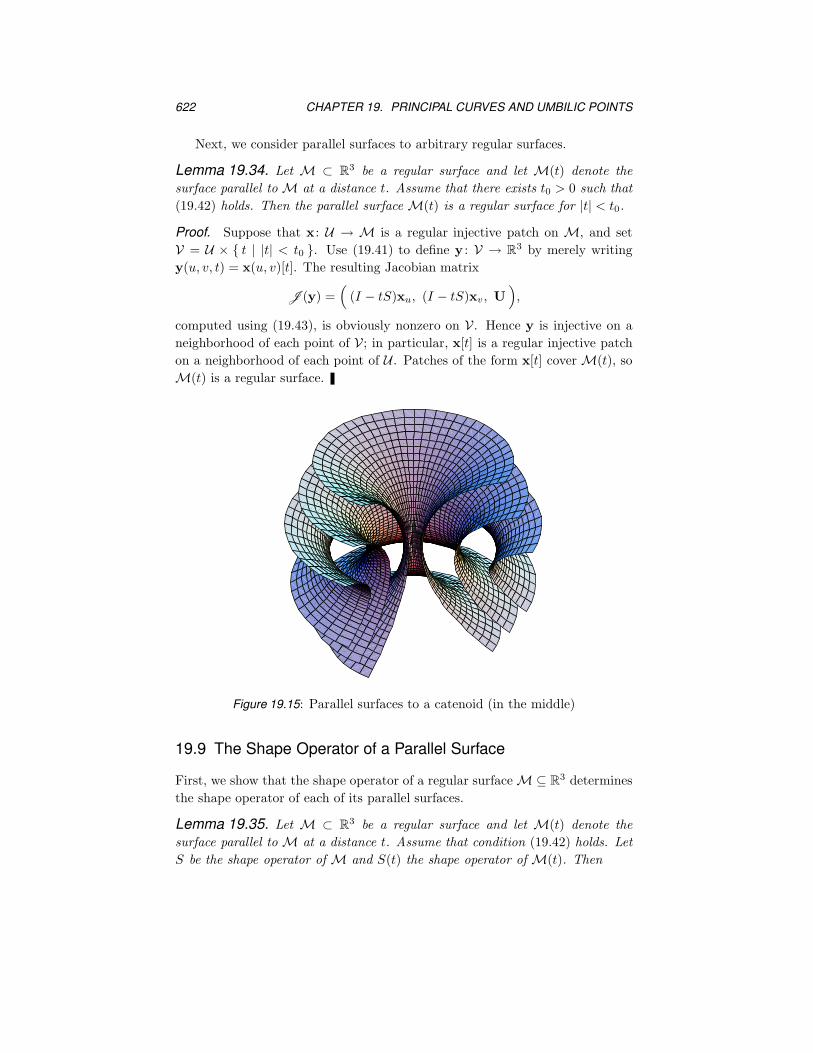
622 CHAPTER 19. PRINCIPAL CURVES AND UMBILIC POINTS
Next, we consider parallel surfaces to arbitrary regular surfaces.
Lemma 19.34. Let M ⊂ R3 be a regular surface and let M(t) denote the
surface parallel to M at a distance t. Assume that there exists t0 > 0 such that
(19.42) holds. Then the parallel surface M(t) is a regular surface for |t| < t0.
Proof. Suppose that x : U → M is a regular injective patch on M, and set
V = U × { t | |t| < t0 }. Use (19.41) to define y : V → R3 by merely writing
y(u, v, t) = x(u, v)[t]. The resulting Jacobian matrix
J(y) =(
(I − tS)xu, (I − tS)xv, U),
computed using (19.43), is obviously nonzero on V . Hence y is injective on a
neighborhood of each point of V ; in particular, x[t] is a regular injective patch
on a neighborhood of each point of U . Patches of the form x[t] cover M(t), so
M(t) is a regular surface.
Figure 19.15: Parallel surfaces to a catenoid (in the middle)
19.9 The Shape Operator of a Parallel Surface
First, we show that the shape operator of a regular surface M ⊆ R3 determines
the shape operator of each of its parallel surfaces.
Lemma 19.35. Let M ⊂ R3 be a regular surface and let M(t) denote the
surface parallel to M at a distance t. Assume that condition (19.42) holds. Let
S be the shape operator of M and S(t) the shape operator of M(t). Then

19.9. SHAPE OPERATOR OF A PARALLEL SURFACE 623
(i) the matrix-valued function t 7→ S(t) satisfies S′(t) = S(t)2;
(ii) S(t) = S(I − tS)−1;
(iii) the principal curvatures of M(t) are given by
ki(t) =ki
1 − tki
,(19.45)
for i = 1, 2, where k1 and k2 are the principal curvatures of M.
(iv) The Gaussian and mean curvatures of M(t) are given by
K(t) =K
1 − 2t H + t2Kand H(t) =
H − t K
1 − 2t H + t2K,(19.46)
where K and H denote the Gaussian and mean curvatures of M.
Proof. Without loss of generality, M is parametrized by a single regular patch
x : U → M. Then the patch x[t] on M(t) defined by (19.41) is regular, with
unit normal
U[t] =x[t]u × x[t]v∥∥x[t]u × x[t]v
∥∥ .
But, given that det(I − tS) > 0, (19.44) implies that U[t] coincides with U.
Therefore,
S(t)x[t]u = −U[t]u = −Uu = Sxu,(19.47)
proving that S(t)x[t]u does not depend on t. Hence
(S(t)x[t]u
)′
= 0,(19.48)
where the prime denotes differentiation with respect to t. Also, from (19.41),
we obtain
x[t]′u = Uu = −Sxu.(19.49)
Then (19.47)–(19.49) imply that
S′(t)x[t]u = −S(t)x[t]′u = S(t)Sxu = S(t)2x[t]u.
Similarly, S′(t)x[t]v = S(t)2x[t]v. Equation (19.44) implies that x[t]u and x[t]vare linearly independent. Hence S′(t) = S(t)2, proving (i).
To prove (ii), we define S(t) = S(I − tS)−1, and use the binomial theorem
to expand it as a convergent geometrical series for small t:
S(t) =∞∑
k=0
tkSk+1.(19.50)

624 CHAPTER 19. PRINCIPAL CURVES AND UMBILIC POINTS
It is clear from (19.50) that S commutes with S(t) for all t, and so
S′(t) = S2(I − tS)−2 = S(t)2.
Since S(0) = S, we conclude that S coincides with S.
For (iii) we compute the eigenvalues of S(I − tS)−1 and use (ii). To prove
(iv), we use (19.45). In particular,
K(t) = k1(t)k2(t) =k1k2
(1 − t k1)(1 − t k2)=
K
1 − 2tH + t2K
and calculation of H(t) is similar .
Now we can prove an important result due to Bonnet. As Chern has re-
marked (see [Chern3]), this theorem tells us that finding surfaces of constant
mean curvature is equivalent to finding surfaces of constant positive Gaussian
curvature.
Theorem 19.36. (Bonnet) Let M ⊂ R3 be a regular surface.
(i) If M has constant mean curvature H ≡ 1/(2c), then the parallel surface
M(c) has constant Gaussian curvature 1/c2, and the parallel surface M(2c) has
constant mean curvature −1/(2c).
(ii) If M has constant Gaussian curvature K ≡ 1/c2, then the parallel sur-
faces M(±c) have constant mean curvature ∓1/(2c).
Proof. If H ≡ 1/(2c), then it follows from (19.46), that
K(c) =K
1 − 2c/(2c) + K c2=
1
c2.
The rest of (i) and (ii) follow from (19.46) in a similar fashion (see Exercise 15).
Finally, we prove a partial converse to Theorem 19.36.
Theorem 19.37. Let M ⊂ R3 be a regular surface with constant positive
Gaussian curvature 1/a2, where a > 0. Let M(t) denote the surface parallel
to M at a distance t. Suppose that the umbilic points of M are isolated. If
M(t) has constant mean curvature, then t = ±a.
Proof. Fix t, and suppose that H(t) is constant on M(t). The second equation
of (19.46) implies that
k1(1 − tk2) + k2(1 − tk1) = 2H(t)(1 − tk1)(1 − tk2),
or
k1 + k2 −2t
a2= 2H(t)
(1 − t(k1 + k2) +
t2
a2
).

19.10. EXERCISES 625
Hence
(k1 + k2)(1 + 2tH(t)
)= 2H(t) + 2H(t)
t2
a2+
2t
a2.(19.51)
By hypothesis, the right-hand of (19.51) is constant. But if the left-hand of
(19.51) is constant, Lemma 19.12 forces it to vanish at the nonumbilic points of
M. Hence 1 + 2tH(t) = 0 everywhere, and (19.51) now implies that
0 = 2H(t)(1 +
t2
a2
)+
2t
a2= −1
t
(1 +
t2
a2
)+
2t
a2= −1
t+
t
a2.
Therefore, t = ±a.
We shall investigate surfaces with constant nonzero Gaussian curvature in
Chapter 21.
19.10 Exercises
1. Prove the second equation of (19.8).
2. Verify that if x : U → R3 is a regular patch, then
∂Γ111
∂v− ∂Γ1
12
∂u− Γ2
12Γ112 + Γ2
11Γ122 = −FK,
as stated in the proof of Theorem 19.8.
3. Prove Corollary 19.10.
4. The Peterson–Mainardi–Codazzi equations also simplify for an asymptotic
patch x : U → R3 (see page 561). Show that
∂ log f
∂u= Γ1
11 − Γ212,
∂ log f
∂v= Γ2
22 − Γ112.
5. Find a patch x : U → R3 for which the coefficients of the first and second
fundamental forms are
E = a2 cos2v, F = 0, G = a2,
e = −a cos2v, f = 0, g = −a.
6. Find a patch x : U → R3 for which the coefficients of the first and second
fundamental forms are
E = a2, F = 0, G = 1,
e = −a, f = 0, g = 0.

626 CHAPTER 19. PRINCIPAL CURVES AND UMBILIC POINTS
7. Find the most general patch x : U → R3 for which xuv = 0.
8. Show that there is no patch having du2 + dv2 and du2 − dv2 as its first
and second fundamental forms.
9. Show that there is no patch having du2 +cos2udv2 and cos2udu2 + dv2 as
its first and second fundamental forms.
10. Let p be a point of an open set U in R2 at which a patch x : U → R
3
satisfies
f E = eF, gE = eG and gF = f G.
Show that there exists a number k such that at p we have
e = kE f = kF and g = kG.
M 11. Show that the surface of revolution generated by a parallel curve β to a
curve α is the same as a parallel surface y to the surface of revolution x
generated by α.
12. The notion of a system of orthogonal curves in R2 corresponds to the
notion of a system of triply orthogonal surfaces in R3:
Definition 19.38. An orthogonal system of curves on an open set U of R2
consists of two families A, B, of curves such that
(i) each point of U lies on one and only one member of each family;
(ii) each curve in each family meets every member of the other family
orthogonally.
Let U ⊆ R2 be an open subset and u = u(x, y), v = v(x, y) two functions
defined on U so that (x, y) 7→ (u, v) is a regular patch U → R2. Suppose
that the partial derivatives of u, v satisfy
ux = vy , uy = −vx.(19.52)
Show that the images of the families H and V of horizontal and vertical
lines in R2 constitute a system of orthogonal curves.
M 13. In the previous exercise, (19.52) are the so-called Cauchy-Riemann equa-
tions that express the fact that u+iv is a holomorphic function (such func-
tions will be discussed in Section 22.1). Use methods from Notebook 19
to study the case in which u+ iv = tan(x+ iy), illustrated in Figure 19.16.

19.10. EXERCISES 627
Figure 19.16: Image of horizontal and vertical lines by z 7→ tan z
Figure 19.17: Orthogonal ellipsoid and hyperboloid of revolution
14. Let A and B be a system of orthogonal curves in R2 that are symmetric
with respect to reflection in a line `. Let A and B be the families of
surfaces of revolution in R3 generated by A and B, using ` as axis (see
Figure 19.17). Show that A and B, together with the family C of planes
through `, constitute a triply orthogonal system of surfaces.
15. Complete the proof of Theorem 19.36.
Related Documents