Principal Components Analysis and Exploratory Factor Analysis · GRI5 2 I find it necessary to gamble with larger amounts of money (than when I first gambled) for gambling to be exciting.

Principal Components Analysis and Exploratory Factor Analysis

PSYC 943 (930): Fundamentals of Multivariate Modeling

Lecture 24: November 30, 2012

PSYC 943: Lecture 24

Today’s Class

• “Advanced” matrix operations

• Principal Components Analysis

• Methods for exploratory factor analysis (EFA) Principal Components-based (TERRIBLE)

PSYC 943: Lecture 24 2

The Logic of Exploratory Analyses

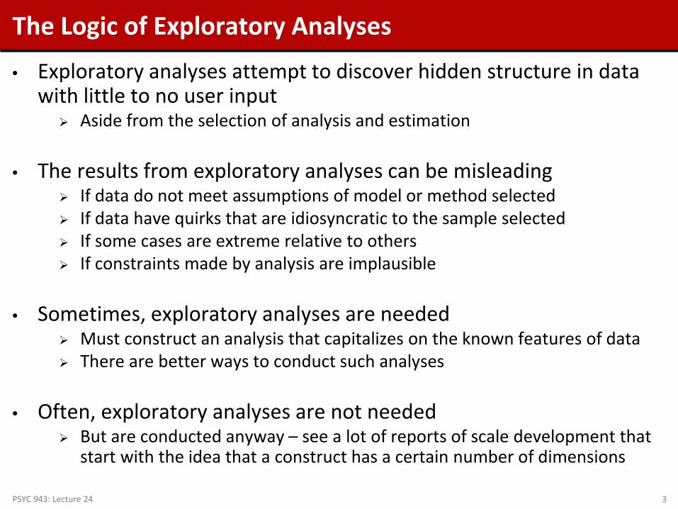
• Exploratory analyses attempt to discover hidden structure in data with little to no user input Aside from the selection of analysis and estimation

• The results from exploratory analyses can be misleading

If data do not meet assumptions of model or method selected If data have quirks that are idiosyncratic to the sample selected If some cases are extreme relative to others If constraints made by analysis are implausible

• Sometimes, exploratory analyses are needed

Must construct an analysis that capitalizes on the known features of data There are better ways to conduct such analyses

• Often, exploratory analyses are not needed

But are conducted anyway – see a lot of reports of scale development that start with the idea that a construct has a certain number of dimensions


ADVANCED MATRIX OPERATIONS


A Guiding Example

• To demonstrate some advanced matrix algebra, we will make use of some data

• I collected data SAT test scores for both the Math (SATM) and Verbal (SATV) sections of 1,000 students

• The descriptive statistics of this data set are given below:


Matrix Trace

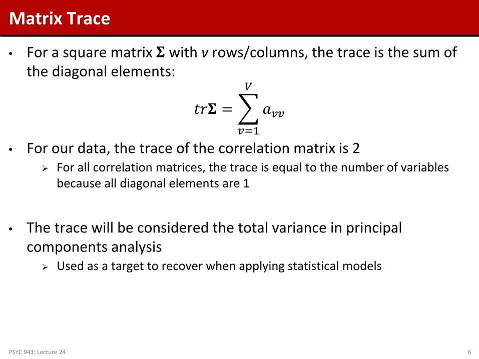
• For a square matrix 𝚺 with v rows/columns, the trace is the sum of the diagonal elements:

𝑡𝑡𝚺 = �𝑎𝑣𝑣

𝑉

𝑣=1

• For our data, the trace of the correlation matrix is 2 For all correlation matrices, the trace is equal to the number of variables

because all diagonal elements are 1

• The trace will be considered the total variance in principal

components analysis Used as a target to recover when applying statistical models


Matrix Determinants • A square matrix can be characterized by a scalar value called

a determinant: det 𝚺 = 𝚺

• Calculation of the determinant by hand is tedious

Our determinant was 0.3916 Computers can have difficulties with this calculation (unstable in cases)

• The determinant is useful in statistics:

Shows up in multivariate statistical distributions Is a measure of “generalized” variance of multiple variables

• If the determinant is positive, the matrix is called positive definite

Is invertable

• If the determinant is not positive, the matrix is called non-positive definite

Not invertable PSYC 943: Lecture 24 7

Matrix Orthogonality

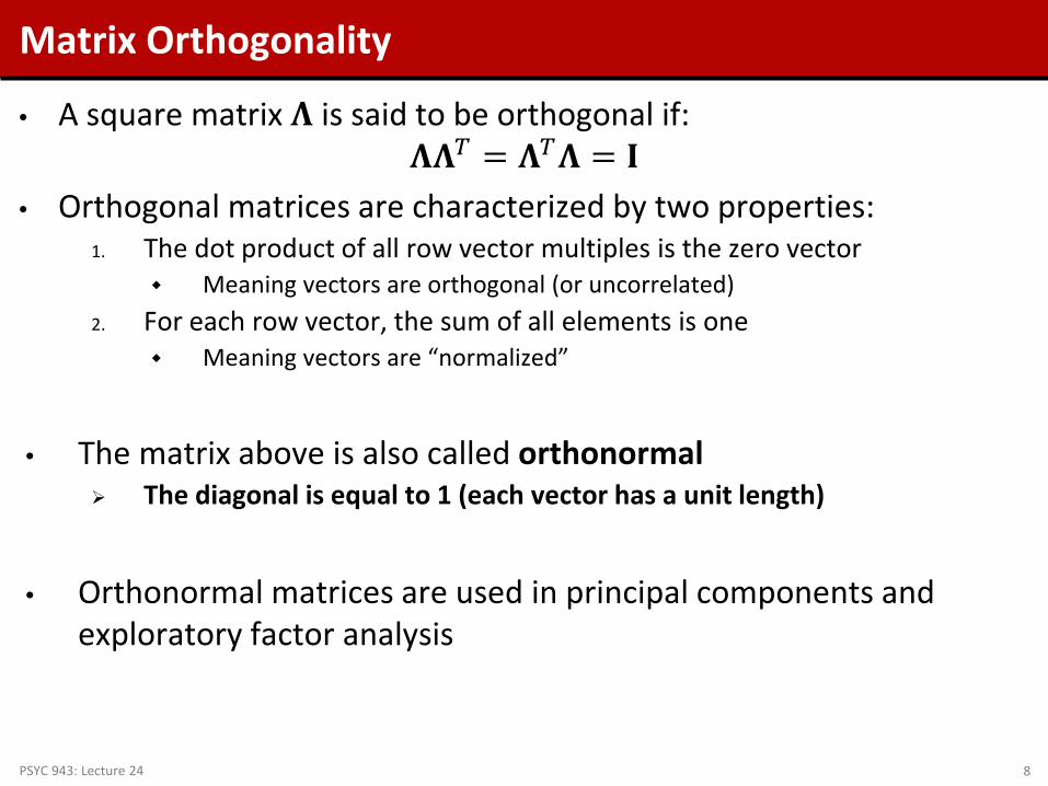
• A square matrix 𝚲 is said to be orthogonal if: 𝚲𝚲𝑇 = 𝚲𝑇𝚲 = 𝐈

• Orthogonal matrices are characterized by two properties: 1. The dot product of all row vector multiples is the zero vector

Meaning vectors are orthogonal (or uncorrelated) 2. For each row vector, the sum of all elements is one

Meaning vectors are “normalized”

• The matrix above is also called orthonormal

The diagonal is equal to 1 (each vector has a unit length)

• Orthonormal matrices are used in principal components and

exploratory factor analysis


Eigenvalues and Eigenvectors

• A square matrix 𝚺 can be decomposed into a set of eigenvalues 𝛌 and a set of eigenvectors 𝐞

𝚺𝐞 = λ𝐞

• Each eigenvalue has a corresponding eigenvector The number equal to the number of rows/columns of 𝚺 The eigenvectors are all orthogonal

• Principal components analysis uses eigenvalues and eigenvectors to

reconfigure data


Eigenvalues and Eigenvectors Example

• In our SAT example, the two eigenvalues obtained were: 𝜆1 = 1.78 𝜆2 = 0.22

• The two eigenvectors obtained were:

𝐞1 = 0.710.71 ; 𝐞2 = 0.71

−0.71

• These terms will have much greater meaning in one moment

(principal components analysis)


Spectral Decomposition

• Using the eigenvalues and eigenvectors, we can reconstruct the original matrix using a spectral decomposition:

𝚺 = �𝜆𝑣𝐞𝑣𝐞𝑣𝑇𝑉

𝑣=1

• For our example, we can get back to our original matrix:

𝐑1 = 𝜆1𝐞1𝐞1𝑇 = 1.78 .71.71 .71 .71 = .89 .89

.89 .89

𝐑2 = 𝐑1 + 𝜆2𝐞2𝐞2𝑇 = .89 .89.89 .89 + 0.22 .71

−.71 .71 −.71

= 1.00 0.780.78 1.00


Additional Eigenvalue Properties

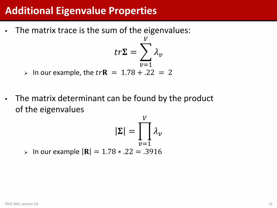
• The matrix trace is the sum of the eigenvalues:

𝑡𝑡𝚺 = �𝜆𝑣

𝑉

𝑣=1

In our example, the 𝑡𝑡𝐑 = 1.78 + .22 = 2

• The matrix determinant can be found by the product

of the eigenvalues

𝚺 = �𝜆𝑣

𝑉

𝑣=1

In our example 𝐑 = 1.78 ∗ .22 = .3916


AN INTRODUCTION TO PRINCIPAL COMPONENTS ANALYSIS


PCA Overview

• Principal Components Analysis (PCA) is a method for re-expressing the covariance (or often correlation) between a set of variables The re-expression comes from creating a set of new variables (linear

combinations) of the original variables

• PCA has two objectives:

1. Data reduction Moving from many original variables down to a few “components”

2. Interpretation

Determining which original variables contribute most to the new “components”


Goals of PCA

• The goal of PCA is to find a set of k principal components (composite variables) that: Is much smaller in number than the original set of V variables Accounts for nearly all of the total variance

Total variance = trace of covariance/correlation matrix

• If these two goals can be accomplished, then the set of k principal

components contains almost as much information as the original V variables Meaning – the components can now replace the original variables in any

subsequent analyses


Questions when using PCA

• PCA analyses proceed by seeking the answers to two questions:

1. How many components (new variables) are needed to “adequately” represent the original data? The term adequately is fuzzy (and will be in the analysis)

2. (once #1 has been answered): What does each component

represent? The term “represent” is also fuzzy


PCA Features

• PCA often reveals relationships between variables that were not previously suspected New interpretations of data and variables often stem from PCA

• PCA usually serves as more of a means to an end rather than an end it itself Components (the new variables) are often used in other

statistical techniques Multiple regression/ANOVA Cluster analysis

• Unfortunately, PCA is often intermixed with

Exploratory Factor Analysis Don’t. Please don’t. Please make it stop.


PCA Details

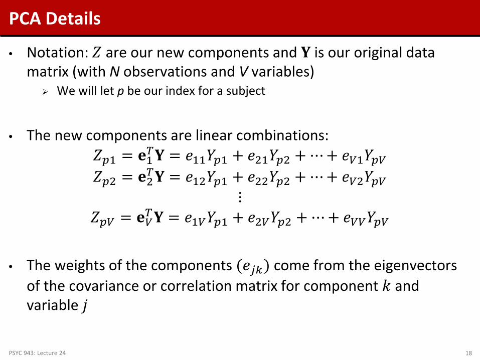
• Notation: 𝑍 are our new components and 𝐘 is our original data matrix (with N observations and V variables) We will let p be our index for a subject

• The new components are linear combinations:

𝑍𝑝1 = 𝐞1𝑇𝐘 = 𝑒11𝑌𝑝1 + 𝑒21𝑌𝑝2 + ⋯+ 𝑒𝑉1𝑌𝑝𝑉 𝑍𝑝2 = 𝐞2𝑇𝐘 = 𝑒12𝑌𝑝1 + 𝑒22𝑌𝑝2 + ⋯+ 𝑒𝑉2𝑌𝑝𝑉

⋮ 𝑍𝑝𝑉 = 𝐞𝑉𝑇𝐘 = 𝑒1𝑉𝑌𝑝1 + 𝑒2𝑉𝑌𝑝2 + ⋯+ 𝑒𝑉𝑉𝑌𝑝𝑉

• The weights of the components (𝑒𝑗𝑗) come from the eigenvectors

of the covariance or correlation matrix for component 𝑘 and variable 𝑗


Details About the Components

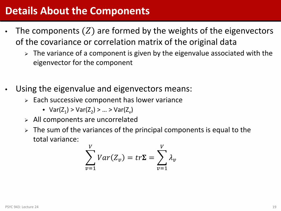
• The components (𝑍) are formed by the weights of the eigenvectors of the covariance or correlation matrix of the original data The variance of a component is given by the eigenvalue associated with the

eigenvector for the component

• Using the eigenvalue and eigenvectors means:

Each successive component has lower variance Var(Z1) > Var(Z2) > … > Var(Zv)

All components are uncorrelated The sum of the variances of the principal components is equal to the

total variance:

�𝑉𝑎𝑡 𝑍𝑣 = 𝑡𝑡𝚺 = �𝜆𝑣

𝑉

𝑣=1

𝑉

𝑣=1


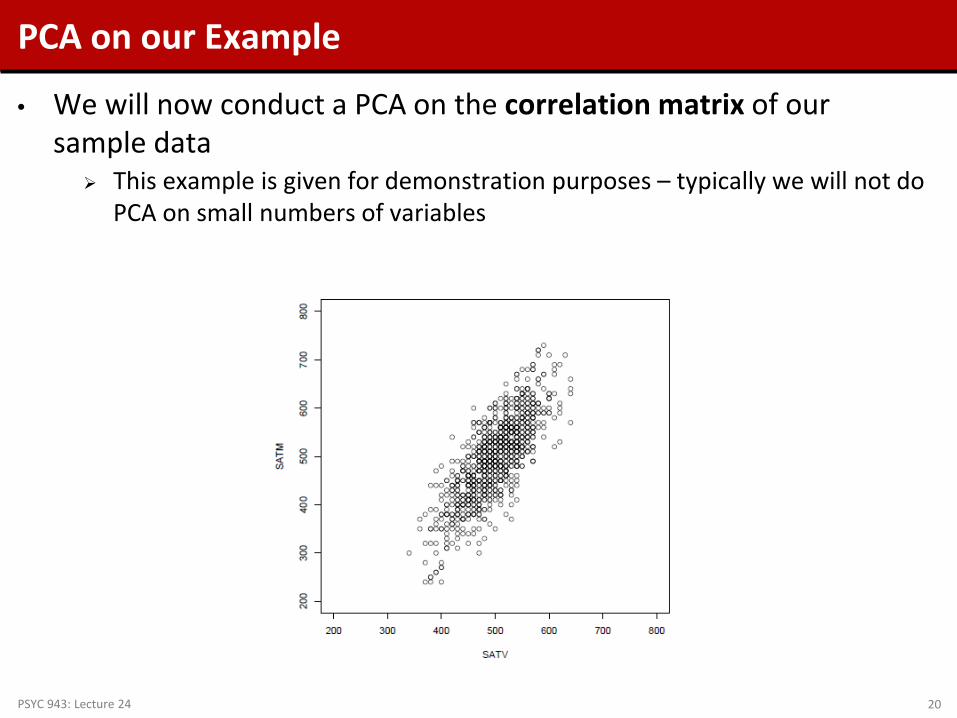
PCA on our Example

• We will now conduct a PCA on the correlation matrix of our sample data This example is given for demonstration purposes – typically we will not do

PCA on small numbers of variables


PCA in SAS

• The SAS procedure that does principal components is called PROC PRINCOMP Mplus does not compute principal components


Graphical Representation

• Plotting the components and the original data side by side reveals the nature of PCA: Shown from PCA of covariance matrix


The Growth of Gambling Access

• In past 25 years: An exponential increase in the

accessibility of gambling An increased rate of with problem

or pathological gambling (Volberg, 2002, Welte et al., 2009)

• Hence, there is a need to better:

Understand the underlying causes of the disorder Reliably identify potential pathological gamblers Provide effective treatment interventions

ERSH 8750: Lecture #5 23

Pathological Gambling: DSM Definition

• To be diagnosed as a pathological gambler, an individual must meet 5 of 10 defined criteria:

ERSH 8750: Lecture #5

1. Is preoccupied with gambling 2. Needs to gamble with increasing

amounts of money in order to achieve the desired excitement

3. Has repeated unsuccessful efforts to control, cut back, or stop gambling

4. Is restless or irritable when attempting to cut down or stop gambling

5. Gambles as a way of escaping from problems or relieving a dysphoric mood

6. After losing money gambling, often returns another day to get even

7. Lies to family members, therapist, or others to conceal the extent of involvement with gambling

8. Has committed illegal acts such as forgery, fraud, theft, or embezzlement to finance gambling

9. Has jeopardized or lost a significant relationship, job, educational, or career opportunity because of gambling

10. Relies on others to provide money to relieve a desperate financial situation caused by gambling

24

Research on Pathological Gambling

• In order to study the etiology of pathological gambling, more variability in responses was needed

• The Gambling Research Instrument (Feasel, Henson, & Jones, 2002) was created with 41 Likert-type items Items were developed to measure each criterion

• Example items (ratings: Strongly Disagree to Strongly Agree):

I worry that I am spending too much money on gambling (C3) There are few things I would rather do than gamble (C1)

• The instrument was used on a sample of experienced gamblers from a riverboat casino in a Flat Midwestern State Casino patrons were solicited after playing roulette


The GRI Items

• The GRI used a 6-point Likert scale 1: Strongly Disagree 2: Disagree 3: Slightly Disagree 4: Slightly Agree 5: Agree 6: Strongly Agree

• To meet the assumptions of factor analysis, we will treat these responses as being continuous This is tenuous at best, but often is the case in factor analysis Later we will discuss how to treat these as categorical items

Hint: Item Response Models


The Sample

• Data were collected from two sources: 112 “experienced” gamblers

Many from an actual casino 1192 college students from a “rectangular” midwestern state

Many never gambled before

• Today, we will combine both samples and treat them as homogenous – one sample of 1304 subjects Later we will test this assumption – measurement invariance (called

differential item functioning in item response theory literature)


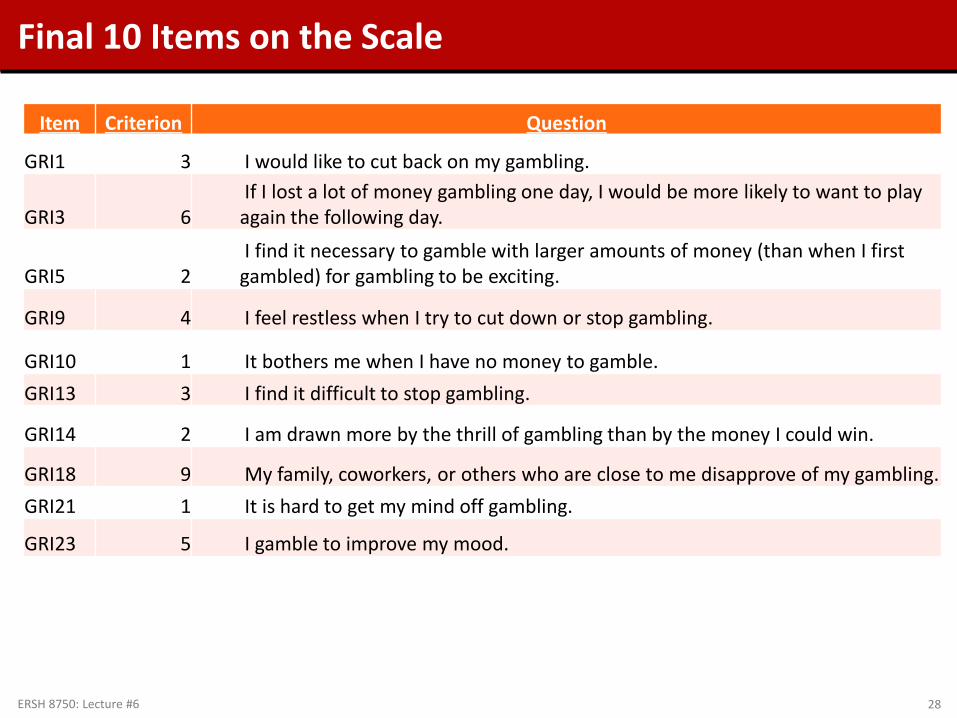
Final 10 Items on the Scale

Item Criterion Question

GRI1 3 I would like to cut back on my gambling.

GRI3 6 If I lost a lot of money gambling one day, I would be more likely to want to play again the following day.

GRI5 2 I find it necessary to gamble with larger amounts of money (than when I first gambled) for gambling to be exciting.

GRI9 4 I feel restless when I try to cut down or stop gambling.

GRI10 1 It bothers me when I have no money to gamble. GRI13 3 I find it difficult to stop gambling.

GRI14 2 I am drawn more by the thrill of gambling than by the money I could win.

GRI18 9 My family, coworkers, or others who are close to me disapprove of my gambling. GRI21 1 It is hard to get my mind off gambling.

GRI23 5 I gamble to improve my mood.


PCA with Gambling Items

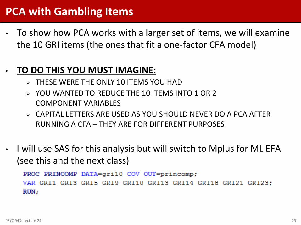
• To show how PCA works with a larger set of items, we will examine the 10 GRI items (the ones that fit a one-factor CFA model)

• TO DO THIS YOU MUST IMAGINE: THESE WERE THE ONLY 10 ITEMS YOU HAD YOU WANTED TO REDUCE THE 10 ITEMS INTO 1 OR 2

COMPONENT VARIABLES CAPITAL LETTERS ARE USED AS YOU SHOULD NEVER DO A PCA AFTER

RUNNING A CFA – THEY ARE FOR DIFFERENT PURPOSES!

• I will use SAS for this analysis but will switch to Mplus for ML EFA (see this and the next class)


Question #1: How Many Components?

• To answer the question of how many components, two methods are used: Scree plot of eigenvalues (looking for the “elbow”) Variance accounted for (should be > 70%)

• We will go with 4 components: (variance accounted for VAC = 75%) • Here variance accounted for is for the total sample variance


Question #2: What Does Each Component Represent? • To answer question #2 – we look at the weights of the eigenvectors

(here is the unrotated solution)


Eigenvectors Prin1 Prin2 Prin3 Prin4

GRI1 0.31 0.10 0.17 0.84 GRI3 0.23 0.08 0.18 0.13 GRI5 0.32 0.09 0.23 -0.03 GRI9 0.24 0.09 0.16 -0.03

GRI10 0.28 0.09 0.24 -0.08 GRI13 0.33 0.16 0.19 -0.22 GRI14 0.45 -0.86 -0.23 -0.01 GRI18 0.35 0.40 -0.83 0.03 GRI21 0.27 0.14 0.06 -0.20 GRI23 0.33 0.10 0.14 -0.42

Final Result: Four Principal Components

• Using the weights of the eigenvectors, we can create four new variables – the four principal components SAS does this for our standardized variables

• Each of these is uncorrelated with each other The variance of each is equal to the corresponding eigenvalue

• We would then use these in subsequent analyses


PCA Summary

• PCA is a data reduction technique that relies on the mathematical properties of eigenvalues and eigenvectors Used to create new variables (small number) out of the old data

(lots of variables) The new variables are principal components (they are not factor scores)

• PCA appeared first in the psychometric literature Many “factor analysis” methods used variants of PCA before likelihood-

based statistics were available

• Currently, PCA (or variants) methods are the default option in SPSS and SAS (PROC FACTOR)


Potentially Solvable Statistical Issues in PCA

• The typical PCA analysis also has a few statistical concerns Some of these can be solved if you know what you are doing The typical analysis (using program defaults) does not solve these

• Missing data is omitted using listwise deletion – biases possible

Could use ML to estimate covariance matrix, but then would have to assume multivariate normality

• The distributions of variables can be anything…but variables with much larger variances will look like they contribute more to each component Could standardize variables – but some can’t be standardized easily

(think gender)

• The lack of standard errors makes the component weights (eigenvector elements) hard to interpret Can use a resampling/bootstrap analysis to get SEs (but not easy to do)


My (Unsolvable) Issues with PCA

• My issues with PCA involve the two questions in need of answers for any use of PCA:

1. The number of components needed is not based on a statistical hypothesis test and hence is subjective Variance accounted for is a descriptive measure No statistical test for whether an additional component significantly

accounts for more variance

2. The relative meaning of each component is questionable at best and hence is subjective Typical packages provide no standard errors for each eigenvector weight

(can be obtained in bootstrap analyses) No definitive answer for component composition

• In sum, I feel it is very easy to be mislead (or purposefully mislead) with PCA


EXPLORATORY FACTOR ANALYSIS


Primary Purpose of EFA

• EFA: “Determine nature and number of latent variables that account for observed variation and covariation among set of observed indicators (≈ items or variables)” In other words, what causes these observed responses? Summarize patterns of correlation among indicators Solution is an end (i.e., is of interest) in and of itself

• Compared with PCA: “Reduce multiple observed variables into

fewer components that summarize their variance” In other words, how can I abbreviate this set of variables? Solution is usually a means to an end


Methods for EFA

• You will see many different types of methods for “extraction” of factors in EFA Many are PCA-based Most were developed before computers became relevant or likelihood

theory was developed

• You can ignore all of them and focus on one:

Only Use Maximum Likelihood for EFA

• The maximum likelihood method of EFA extraction: Uses the same log-likelihood as confirmatory factor analyses/SEM

Default assumption: multivariate normal distribution of data Provides consistent estimates with good statistical properties (assuming you

have a large enough sample) Missing data using all the data that was observed (MAR) Is consistent with modern statistical practices


Questions when using EFA

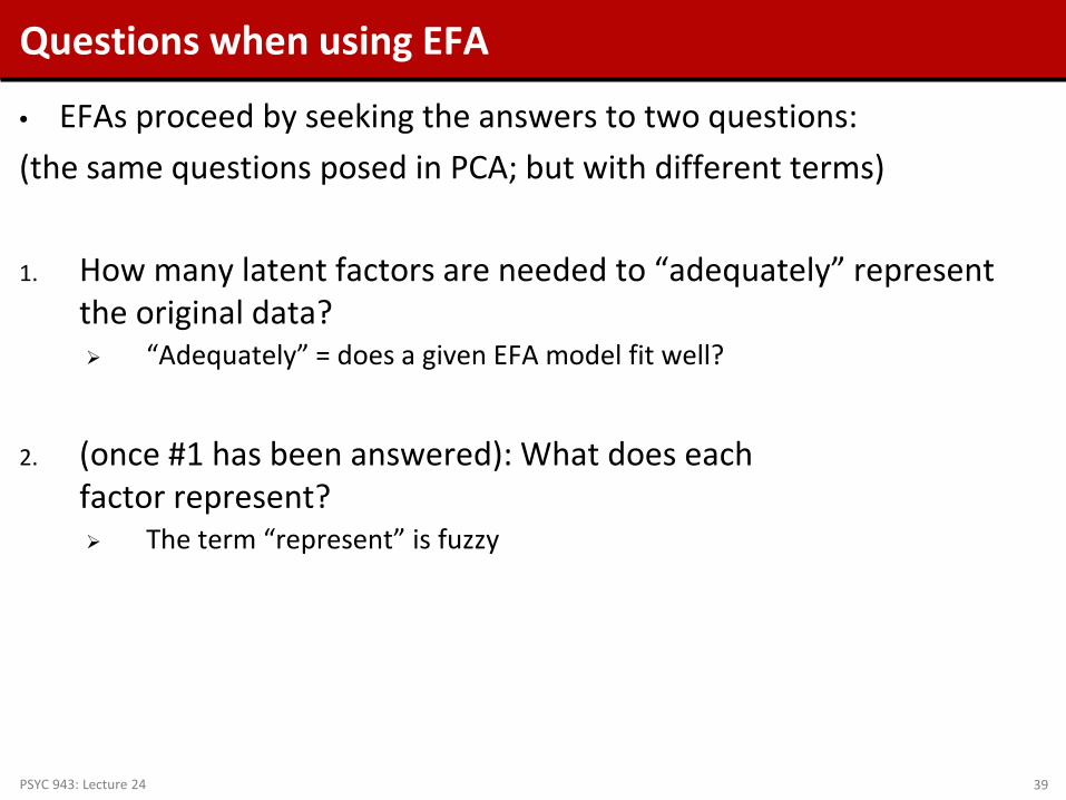
• EFAs proceed by seeking the answers to two questions: (the same questions posed in PCA; but with different terms)

1. How many latent factors are needed to “adequately” represent

the original data? “Adequately” = does a given EFA model fit well?

2. (once #1 has been answered): What does each

factor represent? The term “represent” is fuzzy


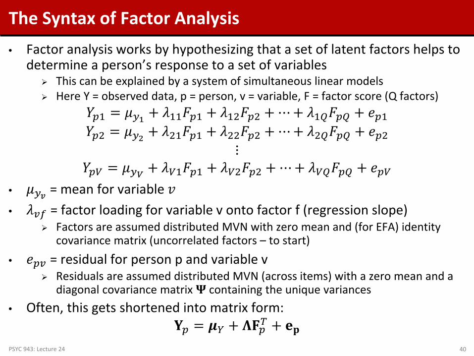
The Syntax of Factor Analysis • Factor analysis works by hypothesizing that a set of latent factors helps to

determine a person’s response to a set of variables This can be explained by a system of simultaneous linear models Here Y = observed data, p = person, v = variable, F = factor score (Q factors)

𝑌𝑝1 = 𝜇𝑦1 + 𝜆11𝐹𝑝1 + 𝜆12𝐹𝑝2 + ⋯+ 𝜆1𝑄𝐹𝑝𝑄 + 𝑒𝑝1 𝑌𝑝2 = 𝜇𝑦2 + 𝜆21𝐹𝑝1 + 𝜆22𝐹𝑝2 + ⋯+ 𝜆2𝑄𝐹𝑝𝑄 + 𝑒𝑝2

⋮ 𝑌𝑝𝑉 = 𝜇𝑦𝑉 + 𝜆𝑉1𝐹𝑝1 + 𝜆𝑉2𝐹𝑝2 + ⋯+ 𝜆𝑉𝑄𝐹𝑝𝑄 + 𝑒𝑝𝑉

• 𝜇𝑦𝑣 = mean for variable 𝑣 • 𝜆𝑣𝑣 = factor loading for variable v onto factor f (regression slope)

Factors are assumed distributed MVN with zero mean and (for EFA) identity covariance matrix (uncorrelated factors – to start)

• 𝑒𝑝𝑣 = residual for person p and variable v Residuals are assumed distributed MVN (across items) with a zero mean and a

diagonal covariance matrix 𝚿 containing the unique variances • Often, this gets shortened into matrix form:

𝐘𝑝 = 𝝁𝑌 + 𝚲𝐅𝑝𝑇 + 𝐞𝐩 PSYC 943: Lecture 24 40

How Maximum Likelihood EFA Works

• Maximum likelihood EFA assumes the data follow a multivariate normal distribution The basis for the log-likelihood function (same log-likelihood we have used

in every analysis to this point)

• The log-likelihood function depends on two sets of parameters: the

mean vector and the covariance matrix Mean vector is saturated (just uses the item means for item intercepts) – so

it is often not thought of in analysis Denoted as 𝝁𝑌 = 𝝁𝐼

Covariance matrix is what gives “factor structure”

EFA models provide a structure for the covariance matrix


The EFA Model for the Covariance Matrix

• The covariance matrix is modeled based on how it would look if a set of hypothetical (latent) factors had caused the data

• For an analysis measuring 𝐹 factors, each item in the EFA: Has 1 unique variance parameter Has 𝐹 factor loadings

• The initial estimation of factor loadings is conducted based on the assumption of uncorrelated factors Assumption is dubious at best –

yet is the cornerstone of the analysis


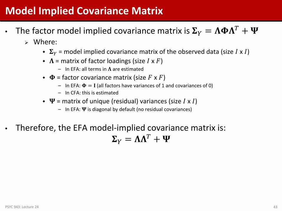
Model Implied Covariance Matrix

• The factor model implied covariance matrix is 𝚺𝑌 = 𝚲𝚲𝚲𝑇 + 𝚿 Where:

𝚺𝑌 = model implied covariance matrix of the observed data (size 𝐼 x 𝐼) 𝚲 = matrix of factor loadings (size 𝐼 x 𝐹)

– In EFA: all terms in 𝚲 are estimated

𝚲 = factor covariance matrix (size 𝐹 x 𝐹) – In EFA: 𝚲 = 𝐈 (all factors have variances of 1 and covariances of 0) – In CFA: this is estimated

𝚿 = matrix of unique (residual) variances (size 𝐼 x 𝐼) – In EFA: 𝚿 is diagonal by default (no residual covariances)

• Therefore, the EFA model-implied covariance matrix is: 𝚺𝑌 = 𝚲𝚲𝑇 + 𝚿


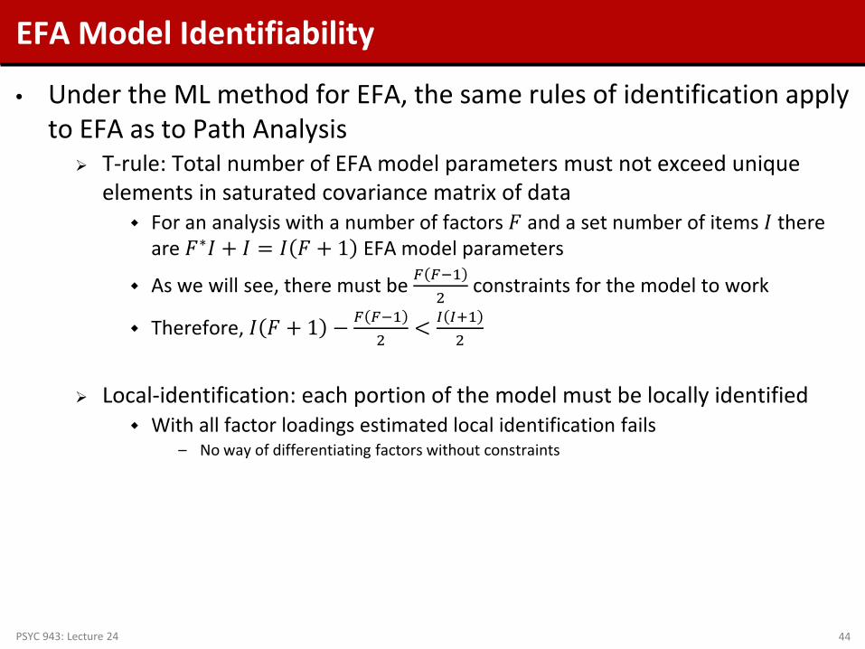
EFA Model Identifiability

• Under the ML method for EFA, the same rules of identification apply to EFA as to Path Analysis T-rule: Total number of EFA model parameters must not exceed unique

elements in saturated covariance matrix of data For an analysis with a number of factors 𝐹 and a set number of items 𝐼 there

are 𝐹∗𝐼 + 𝐼 = 𝐼 𝐹 + 1 EFA model parameters

As we will see, there must be 𝐹 𝐹−12

constraints for the model to work

Therefore, 𝐼 𝐹 + 1 − 𝐹 𝐹−12

< 𝐼 𝐼+12

Local-identification: each portion of the model must be locally identified

With all factor loadings estimated local identification fails – No way of differentiating factors without constraints


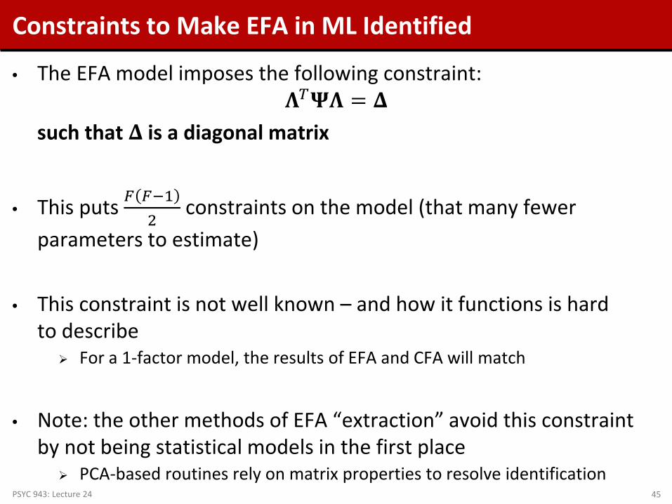
Constraints to Make EFA in ML Identified

• The EFA model imposes the following constraint: 𝚲𝑇𝚿𝚲 = 𝚫

such that 𝚫 is a diagonal matrix

• This puts 𝐹 𝐹−12

constraints on the model (that many fewer parameters to estimate)

• This constraint is not well known – and how it functions is hard

to describe For a 1-factor model, the results of EFA and CFA will match

• Note: the other methods of EFA “extraction” avoid this constraint

by not being statistical models in the first place PCA-based routines rely on matrix properties to resolve identification


The Nature of the Constraints in EFA

• The EFA constraints provide some detailed assumptions about the nature of the factor model and how it pertains to the data

• For example, take a 2-factor model (one constraint):

�𝜓𝑣2�𝜆𝑣𝑣

𝑄=2

𝑣=1

𝑉

𝑣=1

= 0

• In short, some combinations of factor loadings and unique variances

(across and within items) cannot happen This goes against most of our statistical constraints – which must be

justifiable and understandable (therefore testable) This constraint is not testable in CFA


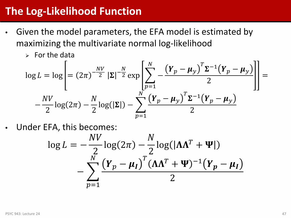
The Log-Likelihood Function

• Given the model parameters, the EFA model is estimated by maximizing the multivariate normal log-likelihood For the data

log𝐿 = log = 2𝜋 −𝑁𝑉2 𝚺 −𝑁2 exp �−𝒀𝑝 − 𝝁𝑦

𝑇𝚺−1 𝒀𝑝 − 𝝁𝑦2

𝑁

𝑝=1

=

−𝑁𝑉2

log 2𝜋 −𝑁2

log 𝚺 −�𝒀𝑝 − 𝝁𝑦

𝑇𝚺−1 𝒀𝑝 − 𝝁𝑦2

𝑁

𝑝=1

• Under EFA, this becomes:

log 𝐿 = −𝑁𝑉2

log 2𝜋 −𝑁2

log 𝚲𝚲𝑇 + 𝚿

−�𝒀𝑝 − 𝝁𝑰

𝑇 𝚲𝚲𝑇 + 𝚿 −1 𝒀𝒑 − 𝝁𝑰2

𝑁

𝑝=1


Benefits and Consequences of EFA with ML

• The parameters of the EFA model under ML retain the same benefits and consequences of any model (i.e., CFA) Asymptotically (large N) they are consistent, normal, and efficient Missing data are “skipped” in the likelihood, allowing for incomplete

observations to contribute (assumed MAR)

• Furthermore, the same types of model fit indices are available in EFA as are in CFA

• As with CFA, though, an EFA model must be a close approximation to the saturated model covariance matrix if the parameters are to be believed This is a marked difference between EFA in ML and EFA with other methods

– quality of fit is statistically rigorous


FACTOR LOADING ROTATIONS IN EFA


Rotations of Factor Loadings in EFA

• Transformations of the factor loadings are possible as the matrix of factor loadings is only unique up to an orthogonal transformation Don’t like the solution? Rotate!

• Historically, rotations use the properties of matrix algebra to adjust the factor loadings to more interpretable numbers

• Modern versions of rotations/transformations rely on “target functions” that specify what a “good” solution should look like The details of the modern approach are lacking in most texts


Types of Classical Rotated Solutions

• Multiple types of rotations exist but two broad categories seem to dominate how they are discussed:

• Orthogonal rotations: rotations that force the factor correlation to zero (orthogonal factors). The name orthogonal relates to the angle between axes of factor solutions being 90 degrees. The most prevalent is the varimax rotation.

• Oblique rotations: rotations that allow for non-zero factor correlations. The name orthogonal relates to the angle between axes of factor solutions not being 90 degrees. The most prevalent is the promax rotation. These rotations provide an estimate of “factor correlation”


How Classical Orthogonal Rotation Works

• Classical orthogonal rotation algorithms work by defining a new rotated set of factor loadings 𝚲∗ as a function of the original (non-rotated) loadings 𝚲 and an orthogonal rotation matrix 𝐓

𝚲∗ = 𝚲𝐓 where: 𝐓𝐓𝑇 = 𝐓𝑇𝐓 = 𝐈 • These rotations do not alter the fit of the model as 𝚺𝑌 = 𝚲∗𝚲∗𝑇 + 𝚿 = 𝚲𝐓 𝚲𝐓 𝑇 + 𝚿 = 𝚲𝐓𝐓𝑇𝚲𝑇 + 𝚿 = 𝚲𝚲𝑇 + 𝚿


Modern Versions of Rotation

• Most studies using EFA use the classical rotation mechanisms, likely due to insufficient training

• Modern methods for rotations rely on the use of a target function for how an optimal loading solution should look


From Browne (2001)

Rotation Algorithms

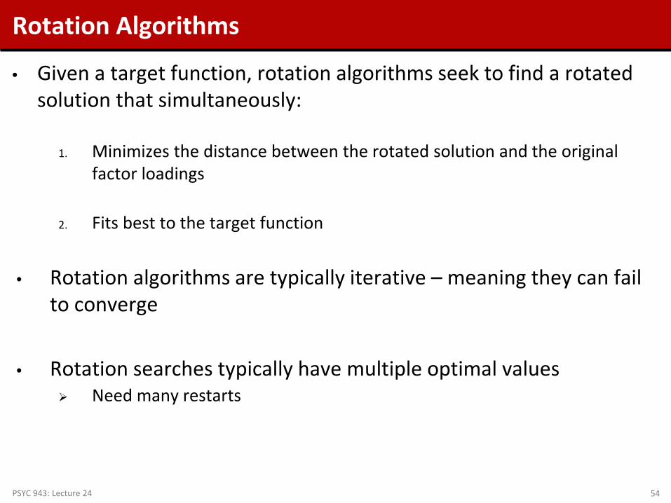
• Given a target function, rotation algorithms seek to find a rotated solution that simultaneously:

1. Minimizes the distance between the rotated solution and the original

factor loadings

2. Fits best to the target function

• Rotation algorithms are typically iterative – meaning they can fail to converge

• Rotation searches typically have multiple optimal values Need many restarts


EFA IN MPLUS


EFA in Mplus

• Mplus has an extensive set of rotation algorithms The default is the Geomin rotation procedure

• The Geomin procedure is the default as it was shown to have a good performance for a classic Thurstone data set (see Browne, 2001)

• We could spend an entire semester on rotations, so I will focus on the default option in Mplus and let the results generalize across most methods


Steps in an ML EFA Analysis

• To determine number of factors: 1. Run a 1-factor model (note: same fit as CFA model)

Check model fit (RMSEA, CFI, TLI) – stop if model fits adequately 2. Run a 2-factor model

Check model fit (RMSEA, CFI, TLI) – stop if model fits adequately 3. Run a 3-factor model (if possible – remember maximum number of

parameters possible) Check model fit (RMSEA, CFI, TLI) – stop if model fits adequately

And so on…

• One huge note: unlike in PCA analyses, there are no model-based eigenvalues to report (nor VAC for the whole model) These are no longer useful in determining the number of factors Mplus will give you a plot (PLOT command, TYPE=PLOT2)

These are from the H1 model correlation matrix


10 Item GRI: EFA Using ML in Mplus

• The 10 item GRI has a 10 10+12

= 55 unique parameters in the H1 (saturated) covariance matrix The limit of parameters possible in an EFA model In theory, we could estimate 6 factors

In practice, 6 factors is impossible with 10 items


Factors Factor Loadings

Unique Variances

Constraints Total Covariance Parameters

1 10 10 0 20

2 20 10 1 29

3 30 10 3 37

4 40 10 6 46

5 50 10 10 50

6 60 10 15 55

Mplus Syntax


Model Comparison: Fit Statistics F Log-Likelihood #Ptrs AIC BIC SSA BIC RMSEA

CFI TLI

1 -16,648.054 30 33,356.108 33,512.031 33,416.735 .052 .969 .961

2 -16,595.511 39 33,269.021 33,471.721 33,347.835 .029 .993 .987

3 -16,581.715 47 33,257.431 33,501.710 33,352.412 .021 .997 .994

4 -16.572.437 54 33,252.873 33,533.535 33,362.001 .000 1.000 1.001

5 -16,568.963 60 33,257.925 33,569.771 33,379.178 .000 1.000 1.004

6 -16.567.438 65 33,264.875 33,602.709 33,396.232 .000 1.000 1.000


Model Comparison: Likelihood Ratio Tests

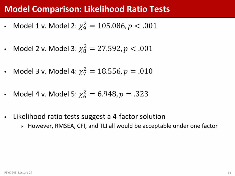
• Model 1 v. Model 2: 𝜒92 = 105.086,𝑝 < .001

• Model 2 v. Model 3: 𝜒82 = 27.592,𝑝 < .001

• Model 3 v. Model 4: 𝜒72 = 18.556,𝑝 = .010

• Model 4 v. Model 5: 𝜒62 = 6.948,𝑝 = .323

• Likelihood ratio tests suggest a 4-factor solution However, RMSEA, CFI, and TLI all would be acceptable under one factor


Mplus Output: A New Warning

• A new warning now appears in the Mplus output:

• .The GEOMIN rotation procedure uses an iterative algorithm that attempts to provide a good fit to the non-rotated factor loadings while minimizing a penalty function It may not converge It may converge to a local minimum It may converge to a location that is not well identified (as is our problem)

• Upon looking at our 4-factor results, we find some very strange numbers So we will stick to the 3-factor model for our explanation In reality you shouldn’t do this (but you shouldn’t do EFA)


Mplus EFA 3-Factor Model Output

• The key to interpreting EFA output is the factor loadings:

• Historically, the standard has been if the factor loading is bigger than .3, then the item is considered to load onto the factor This is different under ML – as we can now use Wald tests


Wald Tests for Factor Loadings

• Using the Wald Tests, we see a different story (absolute value must be great than 2 to be significant)

• Factor 2 has 1 item that significantly loads onto it • Factor 3 has 4 items • Factor 1 has 4 items • Two items have no significant loadings at all


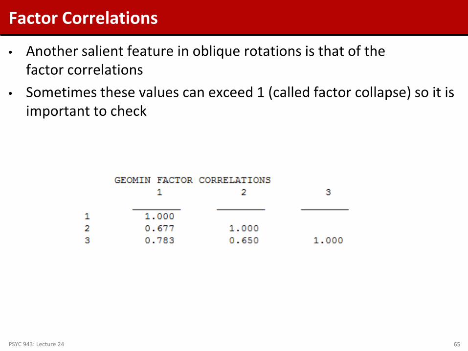
Factor Correlations

• Another salient feature in oblique rotations is that of the factor correlations

• Sometimes these values can exceed 1 (called factor collapse) so it is important to check


Where to Go From Here

• If this was your analysis, you would have to make a determination as to the number of factors We thought 4 – but 4 didn’t work Then we thought 3 – but the solution for 3 wasn’t great Can anyone say 2?

• Once you have settled the number of factors, you must then describe what each factor means Using the pattern of rotated loadings

• After all that, you should validate your result You should regardless of analysis (but especially in EFA)


PCA VERSUS EFA


EFA vs. PCA

• 2 very different schools of thought on exploratory factor analysis (EFA) vs. principal components analysis (PCA):

1. EFA and PCA are TWO ENTIRELY DIFFERENT THINGS…

2. PCA is a special kind (or extraction type) of EFA… although they are often used for different purposes, the results turn out the same a lot anyway, so what’s the big deal?

• My world view: I’ll describe them via school of thought #2

I want you to know what their limitations are I want you to know that they are not really testable models

It is not your data’s job to tell you what constructs you are measuring!! If you don’t have any idea, game over


PCA vs. EFA, continued

• So if the difference between EFA and PCA is just in the communalities (the diagonal of the correlation matrix)… PCA: All variance in indicators is analyzed

No separation of common variance from error variance Yields components that are uncorrelated to begin with

EFA: Only common variance in indicators is analyzed Separates common variance from error variance Yields factors that may be uncorrelated or correlated

• Why the controversy? Why is EFA considered to be about underlying structure,

while PCA is supposed to be used only for data reduction? The answer lies in the theoretical model underlying each…


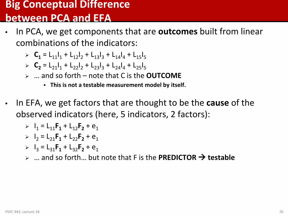
Big Conceptual Difference between PCA and EFA • In PCA, we get components that are outcomes built from linear

combinations of the indicators: C1 = L11I1 + L12I2 + L13I3 + L14I4 + L15I5 C2 = L21I1 + L22I2 + L23I3 + L24I4 + L25I5 … and so forth – note that C is the OUTCOME

This is not a testable measurement model by itself.

• In EFA, we get factors that are thought to be the cause of the observed indicators (here, 5 indicators, 2 factors): I1 = L11F1 + L12F2 + e1 I2 = L21F1 + L22F2 + e1

I3 = L31F1 + L32F2 + e1

… and so forth… but note that F is the PREDICTOR testable


PCA vs. EFA/CFA


Factor

Y1 Y2 Y3 Y4

e1 e2 e3 e4

Component

Y1 Y2 Y3 Y4

This is not a testable measurement model, because how do we know if we’ve combined stuff “correctly”?

This IS a testable measurement model, because we are trying to predict the observed covariances between the indicators by creating a factor – the factor IS the reason for the covariance.

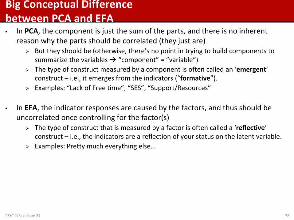
Big Conceptual Difference between PCA and EFA • In PCA, the component is just the sum of the parts, and there is no inherent

reason why the parts should be correlated (they just are) But they should be (otherwise, there’s no point in trying to build components to

summarize the variables “component” = “variable”) The type of construct measured by a component is often called an ‘emergent’

construct – i.e., it emerges from the indicators (“formative”). Examples: “Lack of Free time”, “SES”, “Support/Resources”

• In EFA, the indicator responses are caused by the factors, and thus should be uncorrelated once controlling for the factor(s)

The type of construct that is measured by a factor is often called a ‘reflective’ construct – i.e., the indicators are a reflection of your status on the latent variable.

Examples: Pretty much everything else…


My Issues with EFA

• Often a PCA is done and called an EFA PCA is not a statistical model!

• No statistical test for factor adequacy

• Rotations are suspect

• Constraints are problematic


COMPARING CFA AND EFA


Comparing CFA and EFA

• Although CFA and EFA are very similar, their results can be very different for two or more factors Results for the 1 factor are the same in both (use standardized factor

identification in CFA)

• EFA typically assumes uncorrelated factors

• If we fix our factor correlation to zero, a CFA model becomes very similar to an EFA model But…with one exception…


EFA Model Constraints

• For more than one factor, the EFA model has too many parameters to estimate Uses identification constraints (where 𝚫 is diagonal):

𝚲′𝚿𝚲 = 𝚫

• This puts 𝐹 𝐹−12

multivariate constraints on the model

• These constraints render the comparison of EFA and CFA useless for

most purposes Many CFA models do not have these constraints

• Under maximum likelihood estimators, both EFA and CFA use the same likelihood function Multivariate normal Mplus: full information


CFA Approaches to EFA

• We can conduct exploratory analysis using a CFA model Need to set the right number of constraints for identification We set the value of factor loadings for a few items on a few of the factors

Typically to zero (my usual thought) Sometimes to one (Brown, 2002)

We keep the factor covariance matrix as an identity Uncorrelated factors (as in EFA) with variances of one

• Benefits of using CFA for exploratory analyses: CFA constraints remove rotational indeterminacy of factor loadings – no

rotating is needed (or possible) Defines factors with potentially less ambiguity

Constraints are easy to see For some software (SAS and SPSS), we get much more model

fit information


EFA with CFA Constraints

• To do EFA with CFA, you must: Fix factor loadings (set to either zero or one)

Use “row echelon” form : One item has only one factor loading estimated One item has only two factor loadings estimated One item has only three factor loadings estimated

Fix factor covariances

Set all to 0

Fix factor variances Set all to 1


CONCLUDING REMARKS


Wrapping Up

• Today we discussed the world of exploratory factor analysis and found the following: PCA is what people typically run when they are after EFA

ML EFA is a better option to pick (likelihood based)

Constraints employed are hidden! Rotations can break without you realizing they do

ML EFA can be shown to be equal to CFA for certain models

Overall, CFA is still your best bet

Visit PSYC 948 next semester to learn more about why…


Principal Components Analysis and Exploratory Factor Analysis · GRI5 2 I find it necessary to gamble with larger amounts of money (than when I first gambled) for gambling to be exciting.

Documents