Primal Explicit Max Margin Feature Selection for Nonlinear ...

Primal Explicit Max Margin Feature Selection forNonlinear Support Vector Machines

Aditya Tayala,1,∗, Thomas F. Colemanb,1,2, Yuying Lia,1

aCheriton School of Computer Science, University of Waterloo, Waterloo, ON, Canada N2L 3G1bCombinatorics and Optimization, University of Waterloo, Waterloo, ON, Canada N2L 3G1

Abstract

Embedding feature selection in nonlinear SVMs leads to a challenging non-convex

minimization problem, which can be prone to suboptimal solutions. This paper de-

velops an effective algorithm to directly solve the embedded feature selection primal

problem. We use a trust-region method, which is better suited for non-convex optimiza-

tion compared to line-search methods, and guarantees convergence to a minimizer. We

devise an alternating optimization approach to tackle the problem efficiently, breaking

it down into a convex subproblem, corresponding to standard SVM optimization, and

a non-convex subproblem for feature selection. Importantly, we show that a straight-

forward alternating optimization approach can be susceptible to saddle point solutions.

We propose a novel technique, which shares an explicit margin variable to overcome

saddle point convergence and improve solution quality. Experiment results show our

method outperforms the state-of-the-art embedded SVM feature selection method, as

well as other leading filter and wrapper approaches.

Keywords: nonlinear feature selection, support vector machine, non-convex

optimization, trust-region method, alternating optimization

∗Corresponding authorEmail addresses: [email protected] (Aditya Tayal), [email protected] (Thomas F.

Coleman), [email protected] (Yuying Li)1All three authors acknowledge funding from the National Sciences and Engineering Research Council

of Canada2This author acknowledges funding from the Ophelia Lazaridis University Research Chair. The views

expressed herein are solely from the authors.

Preprint submitted to Elsevier April 10, 2013

1. Introduction

Feature selection has become a significant research focus in statistical machine learning

and data mining communities. As increasingly more data is available, problems with

hundreds and thousands of features have become common. Some examples include text

processing of internet documents, gene micro-array analysis, combinatorial chemistry,

economic forecasting and context based collaborative filtering. However, irrelevant

and redundant features reduce the effectiveness of data mining and may detract from

the quality and accuracy of the resulting model. The goal of feature selection is to

identify the most relevant subset of input features for the learning task, improving

generalization error and model interpretability.

In this paper, we focus on feature selection for nonlinear Support Vector Machine

(SVM) classification. SVM is based on the principle of maximum-margin separation,

which achieves the goal of Structural Risk Minimization by minimizing a generaliza-

tion bound on model complexity and training error concurrently (Cortes and Vapnik,

1995; Vapnik, 1998). The model is obtained by solving a convex quadratic program-

ming problem. Linear SVM models can be extended to nonlinear ones by transform-

ing the input features using a set of nonlinear basis functions. An important advantage

of the SVM is that the transformation can be done implicitly using the “kernel trick”,

thereby allowing even infinite-dimensional feature expansions (Boser et al., 1992). Em-

pirically, SVMs have performed extremely well in diverse domains (e.g. see Byun and

Lee, 2002; Scholkopf et al., 2004).

Determining the optimal set of input features is in general NP-hard, requiring an

exhaustive search of all possible subsets. Practical alternatives can be grouped into

filter, wrapper, and embedded techniques (Guyon and Elisseeff, 2003). Filter meth-

ods operate independently of the SVM classifier to score features according to how

useful they are in predicting the output. Relief (Kira and Rendell, 1992; Sikonja and

Kononenko, 2003) is a popular multivariate nonlinear filter that has successfully been

used as a preprocessing step for SVMs (e.g. see Marchiori, 2005). Wrapper methods,

on the other hand, use the SVM classifier to guide the search in the space of all possible

subsets. For instance the most common wrapper, recursive feature elimination, greed-

2

ily removes the worst (or adds the best) feature according to the loss (or gain) of the

SVM classifier at each iteration (Guyon et al., 2002). Finally, embedded approaches

incorporate the feature selection criterion in the SVM objective itself. Embedded meth-

ods can offer significant advantages over filters and wrappers, since they tightly couple

feature selection with SVM learning, simultaneously searching over the feature and

model space.

For linear SVMs, several embedded feature selection methods have been proposed.

The general idea is to incorporate sparse regularization of the primal weight vector (for

example see Bradley and Mangasarian, 1998; Zhu et al., 2003; Weston et al., 2003;

Fung and Mangasarian, 2004; Chan et al., 2007; Tan et al., 2010). However, similar

techniques cannot be readily applied to nonlinear SVM classifiers, since the weight

vector is not explicitly formed. Sparse regularization of the dual variables (support

vectors) lead to a reduction in the number of kernel functions needed to generate the

nonlinear surface, but does not result in a reduction of input features (Fung and Man-

gasarian, 2004).

Embedding feature selection in a nonlinear SVM requires optimizing over addi-

tional parameters in the kernel function. This can be viewed as an instance of Gener-

alized Multiple Kernel Learning (GMKL) (Varma and Babu, 2009), which offers the

state-of-the-art solution for embedded nonlinear feature selection. However, the re-

sulting problem is non-convex. The algorithm proposed in Varma and Babu (2009) to

solve GMKL is based on gradient descent, i.e. line-search along the negative gradi-

ent. Hence, it uses a first-order convex approximation at each iterate, which can fail to

find a minimizer when the problem is non-convex. In contrast, trust-region algorithms

are better suited for non-convex optimization. At each iterate they solve non-convex

second-order approximations with guaranteed convergence to a minimizer.

This paper develops an effective algorithm to solve the non-convex optimization

problem that results from embedding feature selection in nonlinear SVMs. Our contri-

butions in this paper are as follows:

1. We invoke Representor Theorem to formulate a primal embedded feature selec-

tion SVM problem and use a smoothed hinge loss function to obtain a simpler

3

bound constrained problem. We solve the resulting problem using a generalized

trust-region algorithm for bound constrained minimization.

2. To improve efficiency we propose a two-block alternating optimization scheme,

in which we iteratively solve (a) standard SVM problem and (b) a smaller non-

convex feature selection problem. Importantly, we propose a novel technique

that uses an explicit margin variable, which is shared between subproblems. This

helps avoid suboptimal local minima. Moreover, by focussing on maximizing

margin in the feature selection problem—a critical quantity for generalization

error—we are able to further improve solution quality.

3. We compare our methods to GMKL and other leading nonlinear feature selec-

tors, and show that our approach improves results.

The rest of the paper is organized as follows. Section 2 formulates the embedded

feature selection problem. Section 3 describes the bound constrained trust-region ap-

proach to solve the problem in the full feature and model space. Section 4 develops the

explicit margin alternating optimization approach. Section 5 compares our approach

with other nonlinear feature selection methods on several datasets and we conclude

with a discussion in Section 6.

2. Feature selection in nonlinear SVMs

We start by describing the embedded feature selection problem for nonlinear SVMs.

We motivate and explain the formulation with respect to margin-based generalization

bounds.

Consider a set of n training points, xi ∈ Rd , and corresponding class labels, yi ∈

+1,−1, i = 1, ...,n. Each component of xi is an input feature. In classical SVM,

proposed by Cortes and Vapnik (1995), a linear classifier (w,b) is learned by maximiz-

ing the geometric margin, defined as γ ≡ mini yi(wT xi + b)/‖w‖, where ‖ · ‖ denotes

2-norm. Since the decision hyperplane associated with (w,b) does not change upon

rescaling to (λw,λb), for λ ∈ R+, the function output at the margin (functional mar-

gin) is fixed to 1; geometric margin is given by γ = 1/‖w‖, and the norm of the weight

4

vector is minimized. Thus in the standard setting, SVM results in the following convex

quadratic programming problem:

minw,b,ξ

12‖w‖2 +C

n

∑i=1

ξi,

s.t. yi(wT xi +b

)≥ 1−ξi, i = 1, ...,n, (1)

ξi ≥ 0, i = 1, ...,n .

Here, ξi’s are margin violations, and C is a penalty controlling the trade-off between

empirical error and (implicitly computed) geometric margin.

To obtain a non-linear decision function, the kernel trick (Boser et al., 1992) is

used by defining a kernel function, K(x,x′) ≡ φ(x)Tφ(x′), where K : Rd ×Rd → R

and φ : Rd → F is a non-linear map from input features to a (potentially infinite di-

mensional) derived feature space. A kernel function, satisfying Mercer’s condition

(Mercer, 1909; Courant and Hilbert, 1953), directly computes the inner product of two

vectors in a derived feature space, without the need to explicitly determine the feature

mapping. Conventionally, the kernel is used in the dual of problem (1), where all oc-

currences of data appear inside an inner product. However, we can also formulate the

primal problem in the derived feature space by expressing the weight vector as a linear

combination of mapped data points, w = ∑ni=1 yiuiφ(xi), due to Representer theorem

(Scholkopf and Smola, 2002). We denote the coefficients as ui, and not αi as used in

the standard SVM literature, in order to distinguish them from the typical Lagrange

multiplier interpretation. Substituting this form in (1) leads to the following primal

non-linear SVM problem,

minu,b,ξ

12

n

∑i, j=1

yiy juiu jK(xi,x j)+Cn

∑i=1

ξi,

s.t. yi

(n

∑j=1

y ju jK(xi,x j)+b

)≥ 1−ξi, i = 1, ...,n, (2)

ξi ≥ 0, i = 1, ...,n .

The geometric margin in the derived feature space is given by

γ =1√

∑ni, j=1 yiy juiu jK(xi,x j)

.

5

The dual of problem (2) reveals that the primal variable ui is equivalent to the standard

SVM dual Lagrange multiplier αi, i.e. ui = αi, when the kernel matrix is non-singular.

If the kernel matrix is singular, then the coefficient expansion ui is not unique (even

though the decision function is) and solving (2) will produce one of the possible ex-

pansions, of which αi is also a minimizer.

The maximum margin classifier is motivated by theoretical bounds on the general-

ization error. Specifically, Vapnik (1998) shows that generalization error for n points is

bounded by,

err ≤ cn

[(R2

γ2 +‖ξ‖2)

log2 n+ log1δ

], (3)

for some constant c with probability 1−δ , where γ is the geometric margin of the clas-

sifier. The key expression, on which generalization depends, is R2/γ2 + ‖ξ‖2, where

ξ is the margin slack vector (normalized by γ), and R is the radius of the ball that en-

closes the set of points in the derived feature space, φ(xi)ni=1. For a fixed dataset and

kernel choice, R is constant, and thus maximizing the margin while reducing margin

violations minimizes the upper bound in (3). Although the generalization bound sug-

gests using a 2-norm penalty on margin violations, a 1-norm penalty is preferred for

classification tasks, since it is a better approximation to a step penalty (Vapnik, 1998).

Now consider learning such a classifier while allowing input features to be weighted

according to their relevance. We introduce a feature weight vector, z∈Rd , where zl ≥ 0

is a weight applied to input feature l.3 For convenience we define a diagonal matrix,

Z ∈ Rd×d with Zll = zl . Hence, weighted points are mapped to φ(Zx) and we can re-

place K(x,x′) by K(Zx,Zx′) in problem (2) to obtain the following embedded feature

selection problem, in which we simultaneously search for optimal feature weights, z,

3Without loss of generality, we assume features have been normalized to unit variance

6

while solving for model parameters, (u,b):

minu,b,ξ,z

12

n

∑i, j=1

yiy juiu jK(Zxi,Zx j)+Cn

∑i=1

ξi +µ‖z‖1,

s.t. yi

(n

∑j=1

y ju jK(Zxi,Zx j)+b

)≥ 1−ξi, i = 1, ...,n, (4)

ξi ≥ 0, i = 1, ...,n,

zl ≥ 0, l = 1, ...,d .

We include 1-norm regularization of feature weights, z, with a penalty parameter µ > 0.

This serves two purposes. Firstly, the 1-norm regularizer has the beneficial effect of

suppressing variables to produce a sparse set of non-zero feature weights (Tibshirani,

1996). This property is desirable for feature selection where we are interested in iden-

tifying the most useful subset of input features. Secondly, it acts to minimize the radius

of the enclosing ball, R, for the generalization bound in (3). Given two feature weight

vectors, z and z′, if z′l ≤ zl , for l = 1, ...,d, then ∑l z′2l (xil − x jl)2 ≤ ∑l z2

l (xik − x jl)2,

implying ‖Z′xi−Z′x j‖ ≤ ‖Zxi−Zx j‖. Thus suppressing feature weights reduces dis-

tances between points in input space, which in turn results in a smaller enclosing ball

in feature space. To minimize the generalization bound, we solve (4) and calibrate

margin, errors, and radius via parameters C and µ , which can be determined by cross-

validation.

2.1. Relation to GMKL

We note that problem (4) can be viewed as an instance of generalized multiple kernel

learning (Varma and Babu, 2009). For example, if we consider a radial basis kernel,

then weighting features is equivalent to considering a product of 1-dimensional radial

basis kernels derived from individual features with different width parameters. To solve

this optimization problem Varma and Babu (2009) propose a method based on gradient

descent. The algorithm follows Chapelle et al. (2002) by reformulating the problem

as a nested two step optimization: in an outer loop, the width parameters (i.e. feature

weights) are updated by a line search step along the negative gradient assuming fixed

SVM model parameters, while in an inner loop, the kernel is held fixed and SVM

7

model parameters are updated. Assuming a 1-norm feature weight regularizer, in the

outer loop GMKL solves

minz

F(z)+µ||z||1 subject to zl ≥ 0, l = 1, ...,d (5)

where

F(z) = maxα

n

∑i=1

αi−12

n

∑i, j=1

αiα jyiy jK(Zxi,Zx j)

s.t.n

∑i==1

yiαi = 0, (6)

0≤ αi ≤C, i = 1, ...,n ,

is the solution of the dual SVM problem for fixed feature weights, which is solved

in an inner loop. If α∗ solves (6) exactly, the gradient, ∇zF , can be determined as a

function of optimal α∗ due to Danskin’s Theorem (Danskin, 1967). At each iteration,

a projected Armijo-step (i.e. line search) is taken in the direction of negative gradi-

ent to minimize (5). F(z) is a non-convex function. The gradient descent algorithm

uses a local first-order convex approximation and does not guarantee convergence to

a minimizer in the non-convex case. Moreover, only an approximation to a gradient

is available since the gradient requires an exact solution to the SVM problem, which

computationally cannot be achieved. In contrast, we use a trust region based algo-

rithm to solve the problem, which is better suited for non-convex optimization (4) and

guarantees convergence to a minimizer.

3. Solving the full-space feature selection problem

In this section, we solve the embedded feature selection SVM problem using trust

region algorithm for a bound constrained problem. Problem (4) can be written as:

minu,b,z

Ω(u,b,z) s.t. zl ≥ 0, l = 1, ...,d , (7)

where the objective is expressed in exact-penalty form:

Ω(·) = 12

n

∑i, j=1


∑i=1

V(yi, f (xi)

)+µ‖z‖1 .

8

−1 −0.5 0 0.5 1 1.5 2

0

0.5

1

1.5

2

Output

Lo

ss

Linear hinge

Smoothed hinge

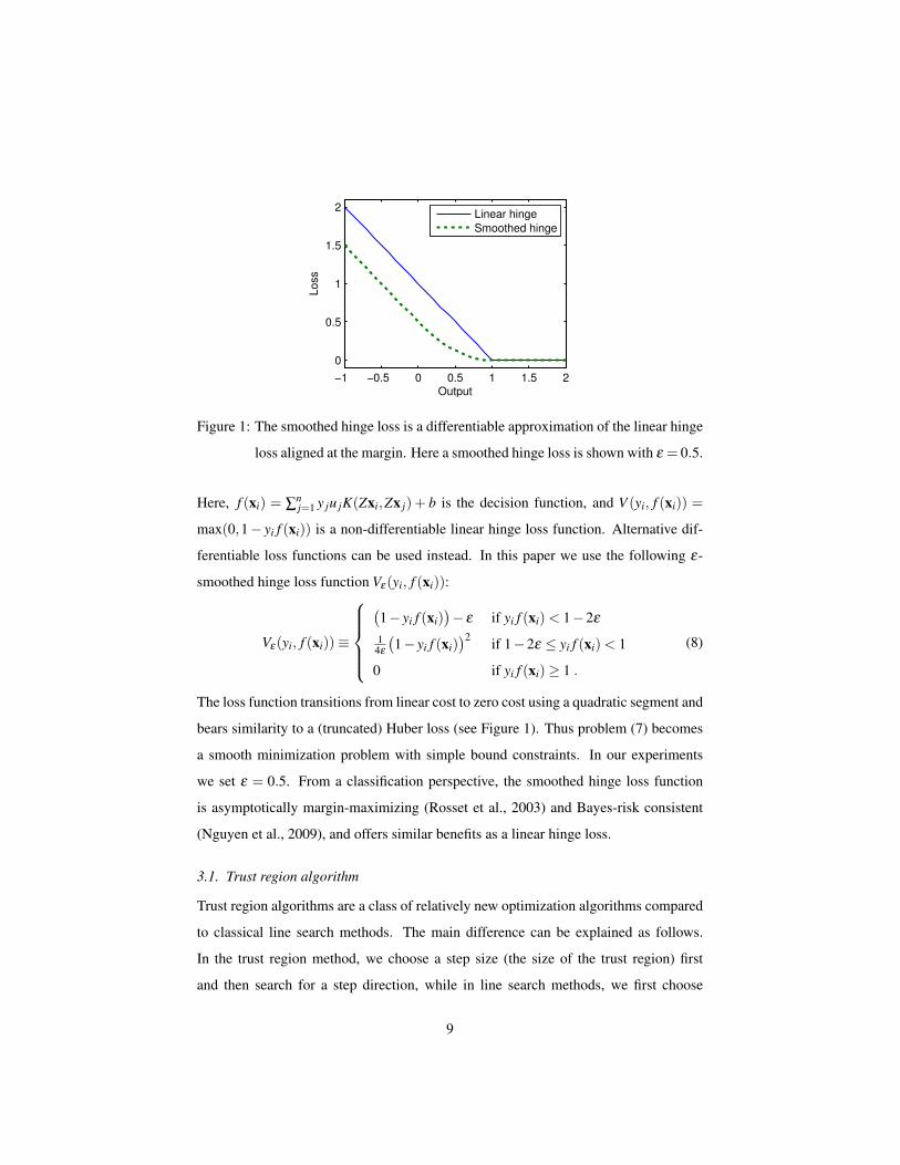
Figure 1: The smoothed hinge loss is a differentiable approximation of the linear hinge

loss aligned at the margin. Here a smoothed hinge loss is shown with ε = 0.5.

Here, f (xi) = ∑nj=1 y ju jK(Zxi,Zx j) + b is the decision function, and V (yi, f (xi)) =

max(0,1− yi f (xi)) is a non-differentiable linear hinge loss function. Alternative dif-

ferentiable loss functions can be used instead. In this paper we use the following ε-

smoothed hinge loss function Vε(yi, f (xi)):

Vε(yi, f (xi))≡

(1− yi f (xi)

)− ε if yi f (xi)< 1−2ε

14ε

(1− yi f (xi)

)2 if 1−2ε ≤ yi f (xi)< 1

0 if yi f (xi)≥ 1 .

(8)

The loss function transitions from linear cost to zero cost using a quadratic segment and

bears similarity to a (truncated) Huber loss (see Figure 1). Thus problem (7) becomes

a smooth minimization problem with simple bound constraints. In our experiments

we set ε = 0.5. From a classification perspective, the smoothed hinge loss function

is asymptotically margin-maximizing (Rosset et al., 2003) and Bayes-risk consistent

(Nguyen et al., 2009), and offers similar benefits as a linear hinge loss.

3.1. Trust region algorithm

Trust region algorithms are a class of relatively new optimization algorithms compared

to classical line search methods. The main difference can be explained as follows.

In the trust region method, we choose a step size (the size of the trust region) first

and then search for a step direction, while in line search methods, we first choose

9

a descent direction and then a step size. The trust region is usually a spherical or

elliptical neighborhood centered at the current iterate, in which a local second order

Taylor expansion (i.e. quadratic approximation) of the objective can be trusted. One

of the main advantages of trust region methods is that a global solution to the local

quadratic model can be computed, even when the Hessian is indefinite (non-convex).

As a result trust region algorithms are better suited for non-convex optimization and

can guarantee convergence to a minimizer.

For unconstrained minimization, the trust region method solves the following sub-

problem to obtain the step-size, s, given the current iterate x(p):

mins∈Rm

sT g(p)+12

sT H(p)s, (9)

s.t. ‖s‖2 ≤ ∆(p).,

Here g(p) and H(p) are the gradient and Hessian of the objective function at x(p), and

∆(p) is the current radius of the trust region. For a nonconvex minimization problem, the

Hessian H(p) can be indefinite and (9) is a nonconvex quadratic minimization problem

with a ball constraint. A global minimizer of this subproblem can be computed since

there is no duality gap for a trust region subproblem. For example, assuming ∆(p) = 1,

the dual of (9) can be solved by first computing a solution to a convex 1-dimensional

problem:

maxυ∈R

−m

∑i=1

(qTi g(p))2

υi +υ−υ ,

s.t. υ ≥−υmin(H(p)) ,

where υi and qi are the eigenvalues and corresponding orthonormal eigenvectors of

H(p), respectively, and υ(H(p)) denotes the minimum eigenvalue of H(p) (Boyd and

Vandenberghe, 2004).

For our implementation, we use the trust region method described in Coleman and

Li (1996), which generalizes the unconstrained case to bound constraints. Each itera-

tion requires an eigen-decomposition of the Hessian matrix involving cubic complex-

ity. Consequently, solving (7) requires O((n+d)3

)operations at each iteration. In the

next section, we propose an explicit margin alternating optimization approach, which

10

improves computation efficiency by breaking the problem down into two smaller sub-

problems, with O(n3) complexity for the SVM subproblem and O(d3) for the feature

selection subproblem, while able to further improve solution quality by avoiding sub-

optimal local minima.

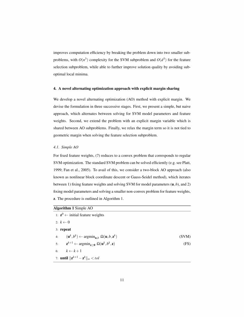
4. A novel alternating optimization approach with explicit margin sharing

We develop a novel alternating optimization (AO) method with explicit margin. We

devise the formulation in three successive stages. First, we present a simple, but naive

approach, which alternates between solving for SVM model parameters and feature

weights. Second, we extend the problem with an explicit margin variable which is

shared between AO subproblems. Finally, we relax the margin term so it is not tied to

geometric margin when solving the feature selection subproblem.

4.1. Simple AO

For fixed feature weights, (7) reduces to a convex problem that corresponds to regular

SVM optimization. The standard SVM problem can be solved efficiently (e.g. see Platt,

1999; Fan et al., 2005). To avail of this, we consider a two-block AO approach (also

known as nonlinear block coordinate descent or Gauss-Seidel method), which iterates

between 1) fixing feature weights and solving SVM for model parameters (u,b), and 2)

fixing model parameters and solving a smaller non-convex problem for feature weights,

z. The procedure is outlined in Algorithm 1.

Algorithm 1 Simple AO

1: z0← initial feature weights

2: k← 0

3: repeat

4: (uk,bk)← argminu,b Ω(u,b,zk) (SVM)

5: zk+1← argminz≥0 Ω(uk,bk,z) (FS)

6: k← k+1

7: until ‖zk+1− zk‖∞ < tol

11

We can use any convex solver for the SVM subproblem and use the bound-constrained

trust-region algorithm described in Section 3.1 to solve the non-convex feature selec-

tion subproblem. The procedure generates a sequence (uk,bk,zk)∞k=1, which can be

shown to converge to a stationary point of (7) (Grippo and Sciandrone, 2000). We stop

when successive changes in feature weights are less than a prespecified tolerance, tol.

Although this simple alternating optimization scheme improves computational effi-

ciency by breaking the problem down into two smaller subproblems, it detracts from an

important advantage of using the trust-region algorithm—convergence to a minimizer.

Even though each subproblem converges to a minimizer when viewed along their re-

stricted subspaces, the solution may not converge to a minimizer in the full variable

space (Bezdek and Hathaway, 2002). A simple example can be illustrative. Consider

minimizing the three-variable quadratic function,

f (x1,x2,x3) = (x1 + x2−2)2−3(x1 + x2−2)(x3−1)+(x3−1)2,

using AO on variable subsets x1,x2 and x3. For fixed x3 = 1, the point (x1,x2) =

(1,1) is a global minimizer of f (x1,x2,1) = (x1 + x2 − 2)2, and for the fixed point

(x1,x2) = (1,1), x3 = 1 is the global minimizer of f (1,1,x3) = (x3 − 1)2. Conse-

quently, AO can converge to (x1,x2,x3) = (1,1,1), which is a stationary point, but not

a minimizer of the full variable space (i.e. it is a saddle point).

Indeed, in our experiments, we find the simple AO scheme is less effective for

non-linear feature selection. We address this shortcoming by introducing an auxiliary

margin variable, which is shared between the two subproblems.

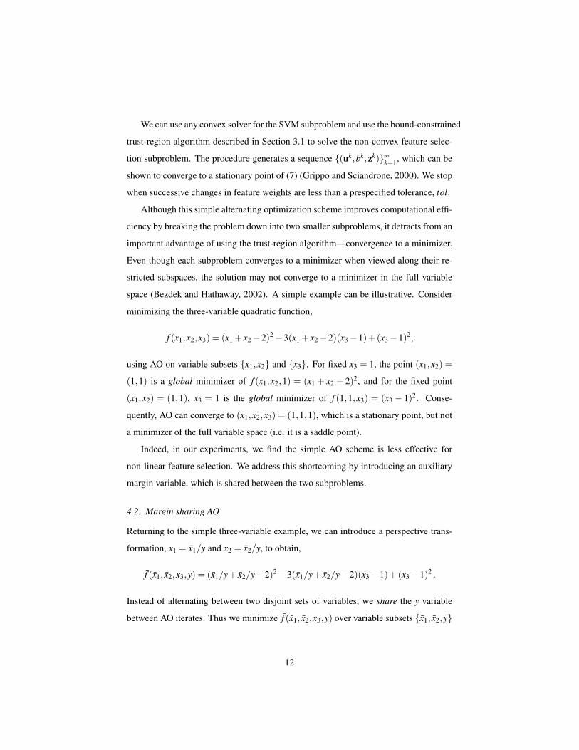
4.2. Margin sharing AO

Returning to the simple three-variable example, we can introduce a perspective trans-

formation, x1 = x1/y and x2 = x2/y, to obtain,

f (x1, x2,x3,y) = (x1/y+ x2/y−2)2−3(x1/y+ x2/y−2)(x3−1)+(x3−1)2 .

Instead of alternating between two disjoint sets of variables, we share the y variable

between AO iterates. Thus we minimize f (x1, x2,x3,y) over variable subsets x1, x2,y

12

and x3,y. For fixed x3 = 1, we minimize f (x1, x2,1,y) = (x1/y+ x2/y−2)2, to ob-

tain a global minimizer (x1, x2,y) = (1,1,1) which corresponds to (x1,y1) = (1,1) as

before. However, for fixed (x1, x2) = (1,1), we now minimize f (1,1,x3,y) = 4(1/y−

1)2− 6(1/y− 1)(x3− 1)+ (x3− 1)2 to find that the Hessian with respect to (x3,y) is

indefinite at (x3,y) = (1,1). Thus by extending the subspace with an auxiliary perspec-

tive variable, which is shared between AO subproblems, we can avoid convergence to

saddle points.

Motivated by this observation, we consider a perspective transformation of SVM

model parameters in the AO approach. We substitute u = u/λ and b = b/λ in (4) to

obtain,

minu,b,ξ,z,λ

12λ 2

n

∑i, j=1


∑i=1

ξi +µ‖z‖1,

s.t. yi

(n

∑j=1

y ju jK(Zxi,Zx j)+ b

)≥ λ −λξi, i = 1, ...,n,

ξi ≥ 0, i = 1, ...,n, (10)

zl ≥ 0, l = 1, ...,d,

λ ≥ 0 .

Note, the auxiliary perspective variable, λ , is equivalent to the functional margin (see

Section 2). We share λ between the AO subproblems. For fixed fixture weights, (10)

is equivalent to a regular SVM, as before (since we fix the functional margin, λ , to

1 to make the problem well-posed). However, in the feature selection subproblem,

when model parameters (u, b) are fixed, λ provides an additional view of the margin

component. This allows us to move along a direction in the SVM model space while

solving the feature selection subproblem. As a result we can avoid convergence to a

saddle point. The procedure is shown in Algorithm 2 using the following exact-penalty

expression for the objective:

Ω(u, b,z,λ ) =1

2λ 2

n

∑i, j=1


∑i=1

V(

yi,f (xi)

λ

)+µ‖z‖1. (11)

We solve the extended feature selection (XFS) subproblem using the bound constrained

trust region algorithm described in Section 3.1. We use z = zk and λ = 1 as initial

13

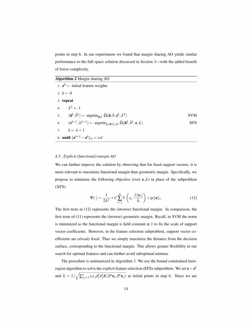
points in step 6. In our experiments we found that margin sharing AO yields similar

performance to the full-space solution discussed in Section 3—with the added benefit

of lower complexity.

Algorithm 2 Margin sharing AO


2: k← 0

3: repeat

4: λ k← 1

5: (uk, bk)← argminu,b Ω(u, b,zk,λ k) SVM

6: (zk+1,λ k+1)← argminz≥0,λ≥0 Ω(uk, bk,z,λ ) XFS

7: k← k+1

8: until ‖zk+1− zk‖∞ < tol

4.3. Explicit (functional) margin AO

We can further improve the solution by observing that for fixed support vectors, it is

more relevant to maximize functional margin than geometric margin. Specifically, we

propose to minimize the following objective (over z,λ ) in place of the subproblem

(XFS).

Ψ(·) = 12λ 2 +C

n

∑i=1

V(

yi,f (xi)

λ

)+µ‖z‖1. (12)

The first term in (12) represents the (inverse) functional margin. In comparison, the

first term of (11) represents the (inverse) geometric margin. Recall, in SVM the norm

is minimized as the functional margin is held constant at 1 to fix the scale of support

vector coefficients. However, in the feature selection subproblem, support vector co-

efficients are already fixed. Thus we simply maximize the distance from the decision

surface, corresponding to the functional margin. This allows greater flexibility in our

search for optimal features and can further avoid suboptimal minima.

The procedure is summarized in Algorithm 3. We use the bound constrained trust-

region algorithm to solve the explicit feature selection (EFS) subproblem. We set z= zk

and λ = 1/√

∑ni, j=1 yiy juk

i ukjK(Zkxi,Zkx j) as initial points in step 6. Since we are

14

mainly interested in feature selection, we use a weaker stopping criteria based on the

zero norm of the weight vector.4 Compared to the full-space approach (Section 3), the

explicit margin AO approach is more efficient. In addition, by focussing on improving

the margin directly—a critical quantity for generalization—it further improves solution

quality.

Algorithm 3 Explicit (functional) margin AO


2: k← 0

3: repeat

4: λ k← 1

5: (uk, bk)← argminu,b Ω(u, b,zk,λ k) SVM

6: (zk+1,λ k+1)← argminz≥0,λ≥0 Ψ(uk, bk,z,λ ) EFS

7: k← k+1

8: until ‖zk+1− zk‖0 = 0

5. Experiments

In this section we evaluate our Full-Space (FULL-FS, Section 3) and AO-Explicit fea-

ture selection (AO-EFS, Section 4.3) methods on various datasets. We compare re-

sults with the state-of-the-art embedded feature selection algorithm, GMKL (Varma

and Babu, 2009). On a simulated dataset (Thompson, 2006) we show that GMKL can

fail to find the correct subset of features, while FULL-FS recovers a better solution

and AO-EFS recovers the correct solution. On several other real datasets we show that

our methods perform better than GMKL by 8-14% on average in terms of test error

and with a reduction of 16-28% of features. We also demonstrate that FULL-FS and

AO-EFS improve upon other leading filter and wrapper approaches in ranking relevant

features.

4In our computation a component is considered zero if its absolute value is less than 0.01×maxk |zk|.

15

5.1. Comparison to GMKL

We optimize features using the same radial-basis kernel when comparing with GMKL.5

K(Zxi,Zx j) = exp

(−

d

∑k=1

(zkxik− zkx jk)2

), (13)

We use a 1-norm penalty on feature weights, µ||z||1, similar to FULL-FS and AO-

EFS. All datasets are standardized to zero mean and unit variance and we always start

with an initial feature weight vector of ones. The two parameters, C and µ , are deter-

mined by cross-validation over (log2 C, log2 µ) space at grid points [−5,−4, ...,14,15]

× [−10,−8, ...,8,10]. We also compare results with regular SVM using the entire set

of features. For SVM we use a radial basis kernel with width σ ,

K(xi,x j) = exp

(−∑

dk=1(xik− x jk)

2

σ2

),

and cross-validate over (log2 C, log2 σ) at [−5,−4, ...,14,15] × [−10,−8, ...,8,10].

5.1.1. Normally Distributed Clusters on Cubes

In this example we evaluate feature selection using a simulated dataset. Normally dis-

tributed clusters on cubes (NDCC) generates nonlinearly separable data by sampling

from multivariate normal distributions with centers at the vertices of three concentric

1-norm cubes (Thompson, 2006). An example with 2-dimensional cubes is shown in

Figure 2. The distribution at each vertex uses a different (randomly generated) covari-

ance matrix. Some centers generate a relatively small number of points, while others

generate a relatively large number of points. Points around opposing vertices of each

cube are assigned to opposite classes preventing linear separation.

In our experiment we generate data at vertices of 20-dimensional cubes and add

100 noisy features by sampling from a normal distribution. Thus the data contains

a total of 120 features of which 20 are informative. This is a challenging dataset for

feature selection because of the high degree of nonlinear interaction among informative

features. Methods which rely on marginal contributions of features will perform poorly

since projection to any single dimension will not reveal class separation.

5Implementation available at http://research.microsoft.com/en-us/um/people/manik/code/gmkl/download.html

16

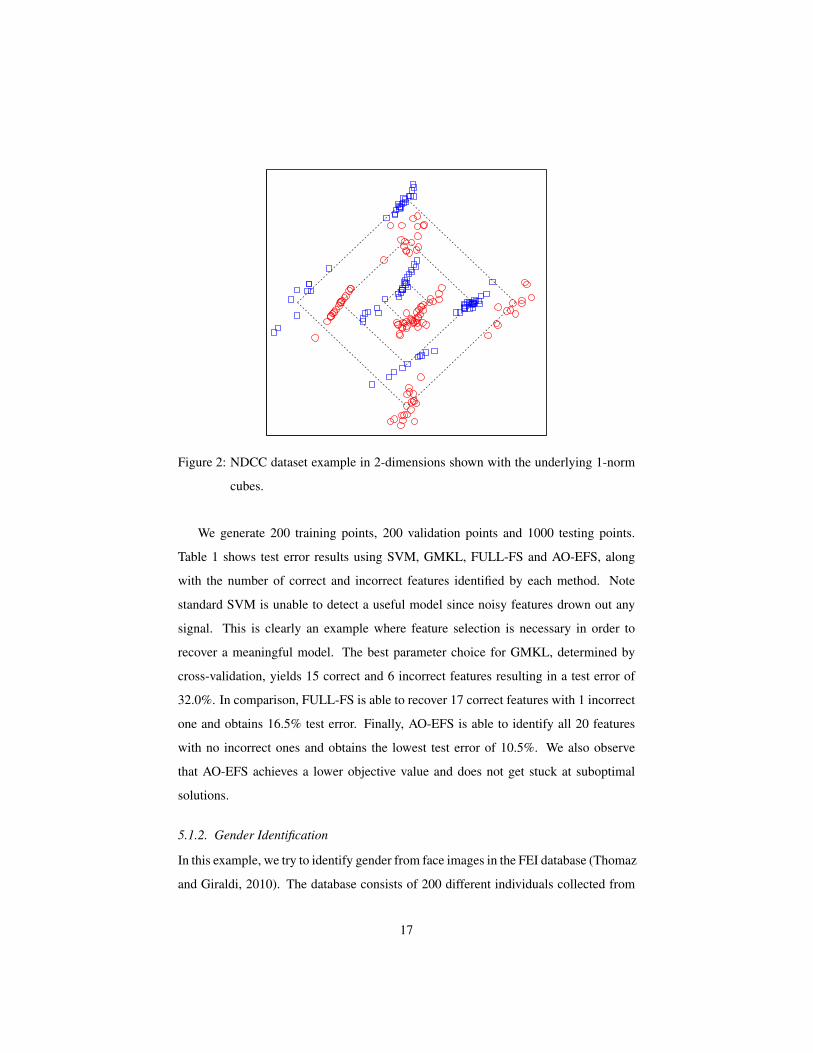
Figure 2: NDCC dataset example in 2-dimensions shown with the underlying 1-norm

cubes.

We generate 200 training points, 200 validation points and 1000 testing points.

Table 1 shows test error results using SVM, GMKL, FULL-FS and AO-EFS, along

with the number of correct and incorrect features identified by each method. Note

standard SVM is unable to detect a useful model since noisy features drown out any

signal. This is clearly an example where feature selection is necessary in order to

recover a meaningful model. The best parameter choice for GMKL, determined by

cross-validation, yields 15 correct and 6 incorrect features resulting in a test error of

32.0%. In comparison, FULL-FS is able to recover 17 correct features with 1 incorrect

one and obtains 16.5% test error. Finally, AO-EFS is able to identify all 20 features

with no incorrect ones and obtains the lowest test error of 10.5%. We also observe

that AO-EFS achieves a lower objective value and does not get stuck at suboptimal

solutions.

5.1.2. Gender Identification

In this example, we try to identify gender from face images in the FEI database (Thomaz

and Giraldi, 2010). The database consists of 200 different individuals collected from

17

Number of Features

Objective Test Error Correct Incorrect

SVM 106.1 44.3% 20 100

GMKL 86.1 32.0% 15 6

FULL-FS 75.2 16.5% 17 1

AO-EFS 62.4 10.5% 20 0

Table 1: 20-dimensional NDCC dataset feature selection results. The objective value,

test error and the number of correct and incorrect features are shown.

students and staff at FEI between the ages of 19 and 40. There are 100 male and 100

female subjects. Each image in the database has been aligned to a common template

so that pixel-wise features correspond roughly to the same location across all subjects.

Images are normalized, equalized, cropped and have been scaled down to have dimen-

sions 18×15. Thus each image consists of 270 pixels of grey scale intensity. Figure 3

shows a few examples from the dataset.

Figure 3: Example of a few processed images in the FEI faces dataset.

We follow standard experimental setup and use 167 images for training and 33 for

out-of-sample testing. Results are averaged over 5 random splits of the data to reduce

variance. Parameters are tuned by running 10-fold cross-validation on the training set

for each split.

Table 2 shows the feature selection results. AO-EFS achieves an error of 11.0%

using on average 16 features. In comparison, FULL-FS achieves an error of 11.9%

using 19 features and GMKL performs comparatively worse with an error of 12.6%

18

using 31 features. Regular SVM obtains an error of 10.8%. SVM results are obtained

using all 270 features. AO-EFS can obtain similar generalization error with approxi-

mately 17 times compression factor. Figure 4 shows the average male and female faces

superimposed with the features identified by GMKL, FULL-FS and AO-EFS.

Test Error(%) Av. # of Features

SVM 10.8 ± 0.8 270.0

GMKL 12.6 ± 1.4 31.4

FULL-FS 11.9 ± 0.9 19.1

AO-EFS 11.0 ± 0.6 16.2

Table 2: Test error and average number of features obtained on the FEI faces dataset.

SVM GMKL FULL-FS AO-EFS

Average

Female

Face

Average

Male

Face

Figure 4: The average male and female faces in the FEI dataset superimposed with the

features identified by GMKL, FULL-FS and AO-EFS. Note that SVM uses

all 270 features.

5.1.3. Other datasets

We compare results on several other datasets obtained from UCI repository (Frank

and Asuncion, 2010). Two-thirds of the observations are used for training and the

remaining one-third for out-of-sample testing. Results are averaged over 5 (stratified)

19

random splits of the data. Parameters are tuned by running 10-fold cross-validation

on the training set for each split. This methodology is used for all datasets, except

Madelon. Madelon was used in the NIPS 2003 Feature Selection Challenge6 and comes

with separate training, validation and testing sets.

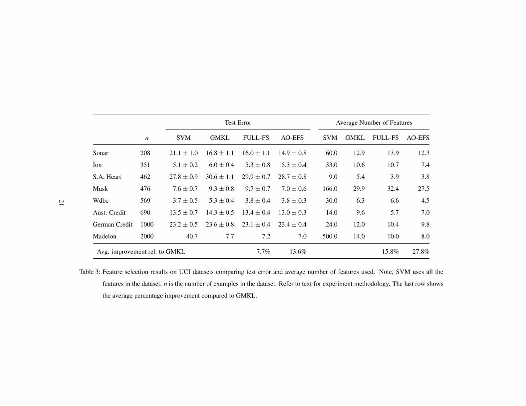
Table 3 summarizes the feature selection results. Average test errors and corre-

sponding average number of features are shown for each dataset. FULL-FS and AO-

EFS improve test error on average by 8% and 14% compared to GMKL, while us-

ing 16% and 28% fewer features, respectively. AO-EFS performs slightly better than

FULL-FS in terms of test error and number of features used. A regular SVM using

uniform feature weights generally yields similar performance, though FULL-FS and

AO-EFS use significantly fewer features. The exception is the Madelon dataset. Made-

lon is constructed specifically to evaluate multivariate feature selection and by design

contains many noisy features, which lead to poor SVM performance.

5.2. Feature Ranking Comparison

In this section we evaluate the ability of FULL-FS and AO-EFS to rank features. We

compare with GMKL as well as three other popular feature selection methods, de-

scribed below:7

• Mutual Information (MI): A filter method, which uses the mutual information

score between candidate features and the output class as a basis to rank features

(Zaffalon and Hutter, 2002). For discrete random variables, mutual information

is given by

I(π) = ∑i

∑j

πi j logπi j

πiπ j,

where πi j is the probability (frequency) of jointly observing events i and j, and

πi = ∑ j πi j and π j = ∑i πi j are the marginal probability of events. Continuous

features are binned to a discrete set corresponding to index i, while j indexes the

6http://www.nipsfsc.ecs.soton.ac.uk/7We use the implementations provided in the Spider machine learning toolbox for these algorithms,

http://people.kyb.tuebingen.mpg.de/spider/.

20

Test Error Average Number of Features

n SVM GMKL FULL-FS AO-EFS SVM GMKL FULL-FS AO-EFS

Sonar 208 21.1 ± 1.0 16.8 ± 1.1 16.0 ± 1.1 14.9 ± 0.8 60.0 12.9 13.9 12.3

Ion 351 5.1 ± 0.2 6.0 ± 0.4 5.3 ± 0.8 5.3 ± 0.4 33.0 10.6 10.7 7.4

S.A. Heart 462 27.8 ± 0.9 30.6 ± 1.1 29.9 ± 0.7 28.7 ± 0.8 9.0 5.4 3.9 3.8

Musk 476 7.6 ± 0.7 9.3 ± 0.8 9.7 ± 0.7 7.0 ± 0.6 166.0 29.9 32.4 27.5

Wdbc 569 3.7 ± 0.5 5.3 ± 0.4 3.8 ± 0.4 3.8 ± 0.3 30.0 6.3 6.6 4.5

Aust. Credit 690 13.5 ± 0.7 14.3 ± 0.5 13.4 ± 0.4 13.0 ± 0.3 14.0 9.6 5.7 7.0

German Credit 1000 23.2 ± 0.5 23.6 ± 0.8 23.1 ± 0.4 23.4 ± 0.4 24.0 12.0 10.4 9.8

Madelon 2000 40.7 7.7 7.2 7.0 500.0 14.0 10.0 8.0

Avg. improvement rel. to GMKL 7.7% 13.6% 15.8% 27.8%

Table 3: Feature selection results on UCI datasets comparing test error and average number of features used. Note, SVM uses all the

features in the dataset. n is the number of examples in the dataset. Refer to text for experiment methodology. The last row shows

the average percentage improvement compared to GMKL.

21

binary class output. Higher values of I(π) imply greater dependence between

the feature and output.

• Relief: A multivariate filter method, which estimates feature relevance by de-

termining how well they distinguish classes between nearby points (Kira and

Rendell, 1992). At each iteration a point is chosen and the weight for each fea-

ture is updated according to the distance of the point to its nearest neighbor from

the same class (hit) and nearest neighbor from the other class (miss). The final

score of a feature is the ratio between the average distance (in projection on that

feature) to the nearest miss and nearest hit over all examples.

• Recursive Feature Elimination (RFE): A wrapper method that uses a greedy

approach to eliminate features, one at a time, that decrease the margin the least

(Guyon et al., 2002). An SVM is trained at each iteration, and the (inverse)

margin is computed: W 2(u)=∑uiu jyiy jK(xi,x j). For each feature l, W 2(−l)(u)=

∑uiu jyiy jK(x−li ,x−l

j ) is computed, where x−li means training point i with feature

l removed. The feature with the smallest value of |W 2(u)−W 2(−l)(u)| is removed.

Repeated application of the procedure results in a ranking of features.

For embedded feature selection methods (i.e. GMKL, FULL-FS, AO-EFS), instead

of varying parameter µ to select the required number of features, we obtain rankings

by taking the top ranked components of z at a fixed C and µ . C and µ are chosen

by cross-validation to minimize classification error. Similar methodology was used by

Varma and Babu (2009).

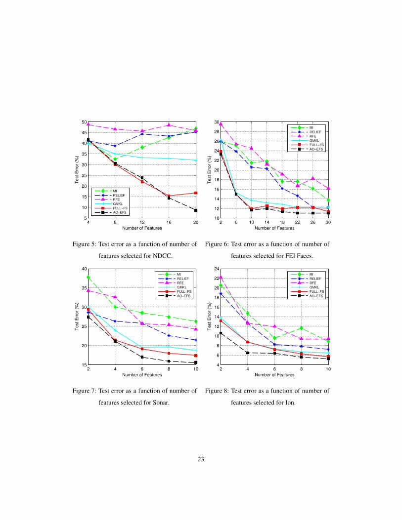
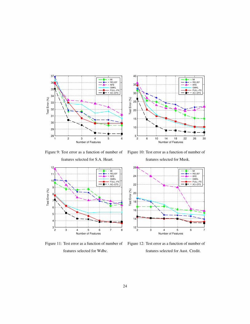
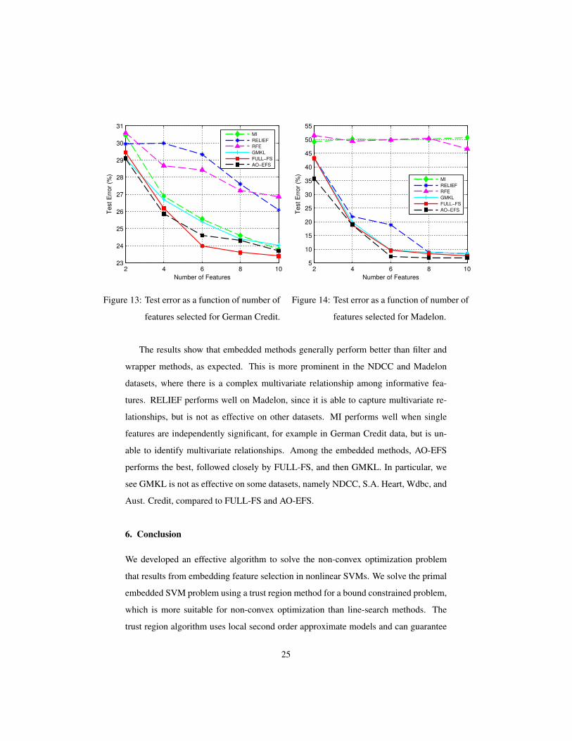
We show test error results versus the number of selected features in Figures 5 to

14. Each figure corresponds to a dataset used in Section 5.1. For a given number of

features, we select the top ranked features and relearn an SVM classifier using only

the selected features. We use a radial basis kernel and cross-validate to determine

optimal SVM parameters, C and σ , for the reduced feature set. Apart from the NDCC

and Madelon datasets, each test error point is obtained by averaging results over five

trials. In each trial, two-thirds of the data is used for training and one-third for testing.

Parameters C and σ are tuned by 10-fold cross-validation on the training set. NDCC

and Madelon use separate training, validation and testing sets.

22

4 8 12 16 205

10

15

20

25

30

35

40

45

50

Number of Features

Te

st

Err

or

(%)

MI

RELIEF

RFE

GMKL

FULL−FS

AO−EFS

Figure 5: Test error as a function of number of

features selected for NDCC.

2 6 10 14 18 22 26 3010

12

14

16

18

20

22

24

26

28

30

Number of Features

Te

st

Err

or

(%)

MI

RELIEF

RFE

GMKL

FULL−FS

AO−EFS


features selected for FEI Faces.

2 4 6 8 1015

20

25

30

35

40

Number of Features

Te

st

Err

or

(%)

MI

RELIEF

RFE

GMKL

FULL−FS

AO−EFS


features selected for Sonar.

2 4 6 8 104

6

8

10

12

14

16

18

20

22

24

Number of Features

Te

st

Err

or

(%)

MI

RELIEF

RFE

GMKL

FULL−FS

AO−EFS


features selected for Ion.

23

1 2 3 4 5 628

29

30

31

32

33

34

35

36

37

Number of Features

Te

st

Err

or

(%)

MI

RELIEF

RFE

GMKL

FULL−FS

AO−EFS


features selected for S.A. Heart.

2 6 10 14 18 22 26 305

10

15

20

25

30

35

40

Number of Features

Te

st

Err

or

(%)

MI

RELIEF

RFE

GMKL

FULL−FS

AO−EFS


features selected for Musk.

2 3 4 5 6 7 83

4

5

6

7

8

9

10

11

12

Number of Features

Te

st

Err

or

(%)

MI

RELIEF

RFE

GMKL

FULL−FS

AO−EFS


features selected for Wdbc.

2 3 4 5 6 712

14

16

18

20

22

24

26

Number of Features

Te

st

Err

or

(%)

MI

RELIEF

RFE

GMKL

FULL−FS

AO−EFS


features selected for Aust. Credit.

24

2 4 6 8 1023

24

25

26

27

28

29

30

31

Number of Features

Te

st

Err

or

(%)

MI

RELIEF

RFE

GMKL

FULL−FS

AO−EFS


features selected for German Credit.

2 4 6 8 105

10

15

20

25

30

35

40

45

50

55

Number of Features

Te

st

Err

or

(%)

MI

RELIEF

RFE

GMKL

FULL−FS

AO−EFS


features selected for Madelon.

The results show that embedded methods generally perform better than filter and

wrapper methods, as expected. This is more prominent in the NDCC and Madelon

datasets, where there is a complex multivariate relationship among informative fea-

tures. RELIEF performs well on Madelon, since it is able to capture multivariate re-

lationships, but is not as effective on other datasets. MI performs well when single

features are independently significant, for example in German Credit data, but is un-

able to identify multivariate relationships. Among the embedded methods, AO-EFS

performs the best, followed closely by FULL-FS, and then GMKL. In particular, we

see GMKL is not as effective on some datasets, namely NDCC, S.A. Heart, Wdbc, and

Aust. Credit, compared to FULL-FS and AO-EFS.

6. Conclusion

We developed an effective algorithm to solve the non-convex optimization problem

that results from embedding feature selection in nonlinear SVMs. We solve the primal

embedded SVM problem using a trust region method for a bound constrained problem,

which is more suitable for non-convex optimization than line-search methods. The

trust region algorithm uses local second order approximate models and can guarantee

25

convergence to a minimizer. For computational efficiency, we apply an alternating op-

timization (AO) framework. We show a naive application of AO can lead to iterates

being trapped at saddle points. We extend the space in which AO is performed with an

auxiliary variable corresponding to the margin. Sharing the margin variable between

AO subproblems reduces saddle point convergence. We further improve solution qual-

ity by directly maximizing the functional margin, instead of the geometric margin, in

the feature selection subproblem. This focusses on maximizing margin, while permit-

ting greater flexibility, as we optimize over the feature space.

We compare our proposed methods to GMKL, the state-of-the-art embedded SVM

feature selection method. GMKL uses a gradient descent algorithm, which does not

guarantee convergence to a minimizer for a non-convex problem and can be susceptible

to suboptimal solutions. On a simulated dataset we show that GMKL can get stuck at

poor solutions and is unable to recover the correct feature subset. On several other real

datasets we show that our methods improve upon GMKL by 8-14% in test error while

further reducing features by 16-28%. We also show how our methods outperform other

leading filter and wrapper approaches in ranking features.

While our algorithm has been described in the context of feature selection, it can

be generalized to non-convex multiple kernel learning. For future work, we hope to

further investigate theoretical and convergence properties of sharing a suitably chosen

auxiliary variable under a block-coordinate AO scheme.

References

Bezdek, J. C., Hathaway, R. J., 2002. Some notes on alternating optimization. In: Pro-

ceedings of the 2002 AFSS International Conference on Fuzzy Systems (AFSS ’02).

pp. 288–300.

Boser, B. E., Guyon, I. M., Vapnik, V. N., 1992. A training algorithm for optimal

margin classifiers. In: Proceedings of the fifth annual workshop on Computational

learning theory. COLT ’92. ACM, pp. 144–152.

Boyd, S., Vandenberghe, L., 2004. Convex Optimization. Cambridge University Press.

26

Bradley, P. S., Mangasarian, O. L., 1998. Feature selection via concave minimization

and support vector machines. In: Machine Learning Proceedings of the Fifteenth

International Conference(ICML 98). pp. 82–90.

Byun, H., Lee, S.-W., 2002. Applications of support vector machines for pattern recog-

nition: A survey. In: Pattern Recognition with Support Vector Machines. pp. 213–

236.

Chan, A. B., Vasconcelos, N., Lanckriet, G. R. G., 2007. Direct convex relaxations

of sparse svm. In: Proceedings of the 24th international conference on Machine

learning. ICML ’07. ACM, pp. 145–153.

Chapelle, O., Vapnik, V., Bousquet, O., Mukherjee, S., 2002. Choosing multiple pa-

rameters for support vector machines. Mach. Learn. 46 (1-3), 131–159.

Coleman, T. F., Li, Y., 1996. An interior trust region approach for nonlinear minimiza-

tion subject to bounds. SIAM Journal on Optimization 6 (2), 415–425.

Cortes, C., Vapnik, V., 1995. Support-vector networks. Machine Learning 20 (3), 273–

297.

Courant, R., Hilbert, D., 1953. Methods of Mathematical Physics. Interscience.

Danskin, J., 1967. The Theory of Max-Min and its Application to Weapons Allocation

Problems.

Fan, R.-E., Chen, P.-H., Lin, C.-J., 2005. Working set selection using second order

information for training support vector machines. Journal of Machine Learning Re-

search 6, 1889–1918.

Frank, A., Asuncion, A., 2010. UCI machine learning repository.

URL http://archive.ics.uci.edu/ml

Fung, G. M., Mangasarian, O. L., 2004. A feature selection newton method for support

vector machine classification. Computational Optimization and Applications 28 (2),

185–202.

27

Grippo, L., Sciandrone, M., 2000. On the convergence of the block nonlinear Gauss-

Seidel method under convex constraints. Operations Research Letters 26, 127–136.

Guyon, I., Elisseeff, A., 2003. An introduction to variable and feature selection. Journal

of Machine Learning Research 3, 1157–1182.

Guyon, I., Weston, J., Barnhill, S., Vapnik, V., 2002. Gene selection for cancer classi-

fication using support vector machines. Machine Learning 46 (1-3), 389–422.

Kira, K., Rendell, L., 1992. A practical approach to feature selection. In: ML92: Pro-

ceedings of the ninth international workshop on Machine learning. pp. 249–256.

Marchiori, E., 2005. Feature selection for classification with proteomic data of mixed

quality. In: In Proceedings of the 2005 IEEE Symposium on Computational Intelli-

gence in Bioinformatics and Computational Biology. pp. 385–391.

Mercer, J., 1909. Functions of positive and negative type and their connection with the

theory of integral equations. Philos. Trans. Royal Soc. (A) 83 (559), 69–70.

Nguyen, X., Wainwright, M. J., Jordan, M. I., 2009. On surrogate loss functions and

f-divergences. Annals of Statistics 37 (2), 876–904.

Platt, J. C., 1999. Advances in kernel methods. MIT Press, Ch. Fast training of support

vector machines using sequential minimal optimization, pp. 185–208.

Rosset, S., Zhu, J., Hastie, T., 2003. Margin maximizing loss functions. In: Advances

in Neural Information Processing Systems (NIPS 15). MIT Press.

Scholkopf, B., Smola, A. J., 2002. Learning with Kernels. MIT Press.

Scholkopf, B., Tsuda, K., Vert, J. P. (Eds.), 2004. Kernel Methods in Computational

Biology. MIT Press.

Tan, M., Wang, L., Tsang, I. W., 2010. Learning sparse svm for feature selection on

very high dimensional datasets. In: Proceedings of the 27th International Conference

on Machine Learning (ICML-10). pp. 1047–1054.

28

Thomaz, C. E., Giraldi, G. A., 2010. A new ranking method for principal components

analysis and its application to face image analysis. Image and Vision Computing

28 (6), 902 – 913.

Thompson, M. E., 2006. NDCC: normally distributed clustered datasets on cubes.

Www.cs.wisc.edu/dmi/svm/ndcc/.

Tibshirani, R., 1996. Regression shrinkage and selection via the lasso. J. Roy. Statist.

Soc. Ser. B 58 (1), 267–288.

Vapnik, V. N., 1998. Statistical Learning Theory, 1st Edition. Wiley.

Varma, M., Babu, B. R., 2009. More generality in efficient multiple kernel learning.

In: Proceedings of the 26th International Conference on Machine Learning (ICML

’09). pp. 1065–1072.

Sikonja, M. R., Kononenko, I., 2003. Theoretical and empirical analysis of ReliefF and

RReliefF. Machine Learning 53 (1-2), 23–69.

Weston, J., Elisseeff, A., Scholkopf, B., Tipping, M., 2003. Use of the zero norm with

linear models and kernel methods. Journal of Machine Learning Research 3, 1439–

1461.

Zaffalon, M., Hutter, M., 2002. Robust feature selection by mutual information dis-

tributions. In: Proceedings of the Eighteenth conference on Uncertainty in artificial

intelligence. UAI’02. pp. 577–584.

Zhu, J., Rosset, S., Hastie, T., Tibshirani, R., 2003. 1-norm support vector machines.

In: Neural Information Processing Systems. Vol. 16.

29

Primal Explicit Max Margin Feature Selection for Nonlinear ...

Documents