Pricing Practices - SU LMS

11

419

We have thus far discussed output and pricing decisions under some verysimplistic assumptions. We have assumed, for example, that a firm is a profitmaximizer, that it produces and sells a single good or service, that all pro-duction takes place in a single location, that the firm operates within a well-defined market structure, and that management has precise knowledgeabout the firm’s production, revenue, and cost functions. In addition, weassumed that the firm sells its output at the same price to all consumers inall markets. These conditions, however, are rarely observed in reality. Thesein the next two chapters we apply the tools of economic analysis developedearlier to more specific real-world situations, including multiplant and multiproduct operations, differential pricing, and non-profit-maximizingbehavior.

PRICE DISCRIMINATION

For firms with market power, price discrimination refers to the practiceof tailoring a firm’s pricing practices to fit specific situations for the purposeof extracting maximum profit. Price discrimination may involve chargingdifferent buyers different prices for the same product or charging the sameconsumer different prices for different quantities of the same product. Pricediscrimination may involve pricing practices that limit the consumers’ability to exercise discretion in the amounts or types of goods and servicespurchased. In whatever guise price discrimination is practiced, it is oftenviewed by the consumer, when the consumer understands what is going on,as somehow nefarious, or at the very least “unfair.”

Pricing Practices

Definition: Price discrimination occurs when profit-maximizing firmscharge different individuals or groups different prices for the same good orservice.

The literature generally discusses three degrees of price discrimination.First-degree price discrimination, which involves charging each individuala different price for each unit of a given product, is potentially the mostprofitable of the three types of price discrimination. First-degree price dis-crimination is the least often observed because of very difficult informa-tional requirements. Second-degree price discrimination differs fromfirst-degree price discrimination in that the firm attempts to maximizeprofits by “packaging” its products, rather than selling each good or serviceone unit at a time. Finally, third-degree price discrimination occurs whenfirms charge different groups different prices for the same good or service.While not as profitable as first-degree and second-degree price discrimina-tion, third-degree price discrimination is the most commonly observed type of differential pricing. A recurring theme in most, but not all, price discriminatory behavior is the attempt by the firm to extract all or someconsumer surplus.

FIRST-DEGREE PRICE DISCRIMINATION

We have noted that price discrimination occurs when different groupsare charged different prices for the same product subject to certain condi-tions. Theoretically, price discrimination could take place at any level ofgroup aggregation. Price discrimination at its most disaggregated leveloccurs when each “group” consists a single individual. First-degree pricediscrimination occurs when firms charge each individual a different pricefor each unit purchased. The price charged for each unit purchased is basedon the seller’s knowledge of each individual’s demand curve. Because it isvirtually impossible to satisfy this informational requirement, first-degreeprice discrimination is extremely rare. Nevertheless, an analysis of first-degree price discrimination is important because it underscores the ratio-nale underlying differential pricing.

Definition: First-degree price discrimination occurs when a seller chargeseach individual a different price for each unit purchased.

The purpose of first-degree price discrimination is to extract the totalamount of consumer surplus from each individual customer. The conceptof consumer surplus was introduced in Chapter 8. Consumer surplus rep-resents the dollar value of benefits received from purchasing an amount ofa good or service in excess of benefits actually paid for. In Figure 11.1, whichillustrates an individual’s demand (marginal benefit) curve for a particularproduct, the market price of the product is $3. At that price, the consumer

420 pricing practices

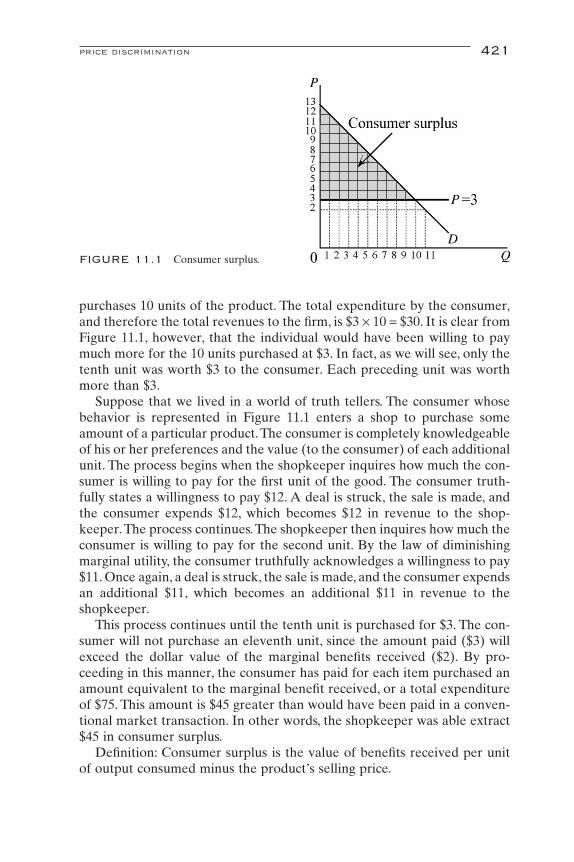
purchases 10 units of the product. The total expenditure by the consumer,and therefore the total revenues to the firm, is $3 ¥ 10 = $30. It is clear fromFigure 11.1, however, that the individual would have been willing to paymuch more for the 10 units purchased at $3. In fact, as we will see, only thetenth unit was worth $3 to the consumer. Each preceding unit was worthmore than $3.

Suppose that we lived in a world of truth tellers. The consumer whosebehavior is represented in Figure 11.1 enters a shop to purchase someamount of a particular product.The consumer is completely knowledgeableof his or her preferences and the value (to the consumer) of each additionalunit. The process begins when the shopkeeper inquires how much the con-sumer is willing to pay for the first unit of the good. The consumer truth-fully states a willingness to pay $12. A deal is struck, the sale is made, andthe consumer expends $12, which becomes $12 in revenue to the shop-keeper.The process continues.The shopkeeper then inquires how much theconsumer is willing to pay for the second unit. By the law of diminishingmarginal utility, the consumer truthfully acknowledges a willingness to pay$11. Once again, a deal is struck, the sale is made, and the consumer expendsan additional $11, which becomes an additional $11 in revenue to the shopkeeper.

This process continues until the tenth unit is purchased for $3. The con-sumer will not purchase an eleventh unit, since the amount paid ($3) willexceed the dollar value of the marginal benefits received ($2). By pro-ceeding in this manner, the consumer has paid for each item purchased anamount equivalent to the marginal benefit received, or a total expenditureof $75. This amount is $45 greater than would have been paid in a conven-tional market transaction. In other words, the shopkeeper was able extract$45 in consumer surplus.

Definition: Consumer surplus is the value of benefits received per unitof output consumed minus the product’s selling price.

price discrimination 421

FIGURE 11.1 Consumer surplus.

Of course, this mind experiment is unrealistic in the extreme. Moreover,the amount of consumer surplus we calculated is only a rough approxima-tion. With the price variations made arbitrarily small, the actual value ofconsumer surplus is the value of the shaded area in Figure 11.1. Our sce-nario, however, underscores the benefits to the firm being able to engagein first-degree price discrimination.

Alas, we do not live in a world of truth tellers. Even if we were com-pletely cognizant of our individual utility functions, we would more thanlikely understate the true value of the next additional unit offered for sale.Moreover, even if the firm knew each consumer’s demand equation, therealities of actual market transactions make it extremely unlikely that thefirm would be able to extract the full amount of consumer surplus. Trans-actions are seldom, if ever, conducted in such a piecemeal fashion.

More formally, for discrete changes in sales (Q), consumer surplus maybe approximated as

(11.1)

where Qn is the quantity demanded by individual i at the market price, Pn. Ifwe assume that the individual’s demand function is linear, that is,

(11.2)

then consumer surplus is approximated as

(11.3)

Examination of Equation (11.3) suggests that the smaller DQ, the betterthe approximation of the shaded area in Figure 11.1. It can be easily demon-strated, and can be seen by inspection, that for a linear demand equation,as DQ Æ 0 the value of the shaded area in Figure 11.1 may be calculatedas

(11.4)

In Chapter 2 we introduced the concept of the integral as accurately rep-resenting the area under a curve. The concept of the integral can be appliedin this instance to calculate the value of consumer surplus. Defining thedemand curve as P = f(Q), consumer surplus may be defined as

where Pn and Qn are the equilibrium price and quantity, respectively. Sub-stituting Equation (11.2) into the integral equation yields

CS f Q dQ P Q= ( ) -Ú * *

CS b P Qn n= -( )0 5 0.

CS b b Q Q P Qi n ni n

= +( ) -= ÆÂ 0 11

D

P b b Qi i= +0 1

CS P Q P Qii n

n n= ¥( ) -= ÆÂ D1


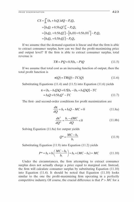
If we assume that the demand equation is linear and that the firm is ableto extract consumer surplus, how can we find the profit-maximizing priceand output level? If the firm is able to extract consumer surplus, totalrevenue is

(11.5)

If we assume that total cost as an increasing function of output, then thetotal profit function is

(11.6)

Substituting Equations (11.4) and (11.5) into Equation (11.6) yields

(11.7)

The first- and second-order conditions for profit maximization are

(11.8a)

(11.8b)

Solving Equation (11.8a) for output yields

(11.9)

Substituting Equation (11.9) into Equation (11.2) yields

(11.10)

Under the circumstances, the firm attempting to extract consumersurplus does not actually charge a price equal to marginal cost. Instead,the firm will calculate consumer surplus by substituting Equation (11.10)into Equation (11.4). It should be noted that Equation (11.10) looks similar to the one the profit-maximizing firm operating in a perfectly competitive industry. Of course, the crucial difference is that P > MC for a

P b bMC b

bb MC b MC* = +

-ÊË

ˆ¯ = + -( ) =0 1

0

10 0

QMC b

b* =

- 0

1

ddQ

b dMCdQ

p2

2

1 0=-

<

ddQ

b b Q MCp

= + - =0 1 0

p = -( ) + - +( )[ ] -= + -

b b Q Q b b b Q Q TC

b Q b Q TC0 1 0 0 1

0 12

0 5

0 5

.

.

p Q TR Q TC Q( ) = ( ) - ( )

TR PQ b P Q= + -( )0 5 0.

CS b b Q dQ P Q

b Q b Q P Q

b Q b Q b b P Q

b Q b Q P Q

i n n

n

i in

n n

n n n n

n n n n

= +( ) -

= +[ ] -

= +[ ] - ( ) + ( )[ ] -

= +[ ] -

Ú 0 10

0 12

0

0 12

0 12

0 12

0 5

0 5 0 0 5 0

0 5

.

. .

.


profit-maximizing firm facing a downward-sloping demand curve for itsproduct.

Problem 11.1. Assume that an individual’s demand equation is

Suppose that the market price of the product is Pn = $6.a. Approximate the value of this individual’s consumer surplus for DQ = 1.b. What is value of consumer surplus as DQ Æ 0?

Solutiona. The equation for approximating the value of consumer surplus for dis-

crete changes in Q when the demand function is linear is

For Pn = $6 and DQ = 1 this equation becomes

For values of Qi from 0 to 7 this becomes

The approximate value of consuming 7 units of this good is approxi-mately $84 dollars. If the consumer pays $6 for 7 units of the good, thenthe individual’s total expenditure is $42. The approximate dollar valueof benefits received, but not paid for, is $42.

b. The value of the individual’s consumer surplus as DQ Æ 0 is given bythe expression

Substituting into this expression we obtain

The actual value of consumer surplus is $49, compared with the approx-imated value of $42 calculated in part a.

SECOND-DEGREE PRICE DISCRIMINATION

Sometimes referred to as volume discounting, second-degree price dis-crimination differs from first-degree price discrimination in the manner inwhich the firm attempts to extract consumer surplus. In the case of second-

CS = -( ) = ( ) =0 5 20 6 7 0 5 14 7 49. . $

CS b P Qn n= -( )0 5 0.

CS = - ( )[ ]+ - ( )[ ]+ - ( )[ ]+ - ( )[ ]+ - ( )[ ]+ - ( )[ ]+ - ( )[ ] -

= + + + + + + - =

20 2 1 20 2 2 20 2 3 20 2 4

20 2 5 20 2 6 20 2 7 42

18 16 14 12 10 8 6 42 42$

CS Qii n

= -( ) -= ÆÂ 20 2 421

CS b b Q Q P Qi n ni n

= +( ) -= ÆÂ 0 11

D

P Qi i= -20 2


degree price discrimination, sellers attempt to maximize profits by sellingproduct in “blocks” or “bundles” rather than one unit at a time. There aretwo common types of second-degree price discrimination: block pricing andcommodity bundling.

Definition: Second-degree price discrimination occurs when firms selltheir product in “blocks” or “bundles” rather than one unit at a time.

Block Pricing

Block pricing, or selling a product in fixed quantities, is similar to first-degree price discrimination in that the seller is trying to maximize profitsby extracting all or part of the buyer’s consumer surplus. Eight frankfurterrolls in a package and a six-pack of beer are examples of block pricing.

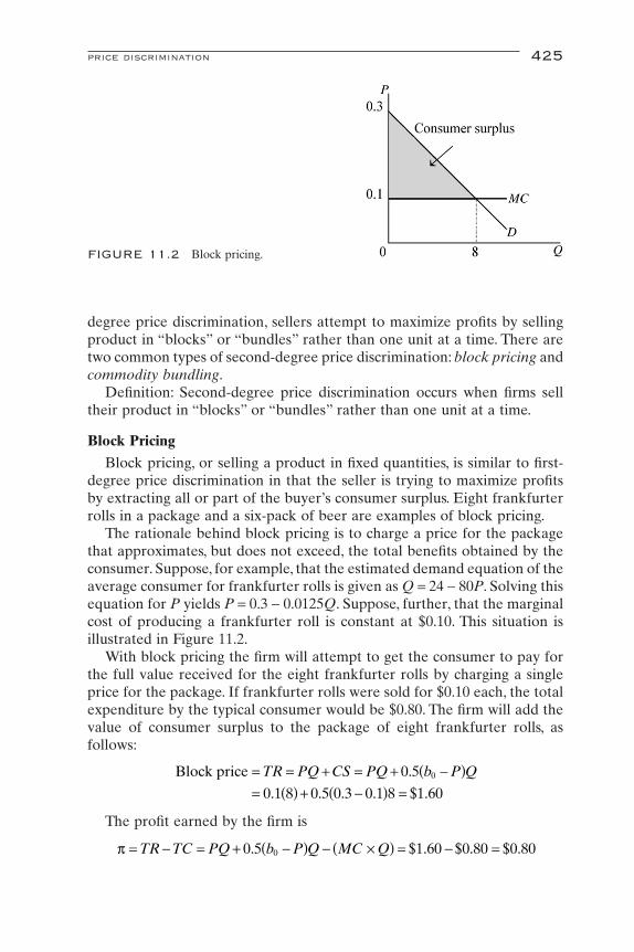
The rationale behind block pricing is to charge a price for the packagethat approximates, but does not exceed, the total benefits obtained by theconsumer. Suppose, for example, that the estimated demand equation of theaverage consumer for frankfurter rolls is given as Q = 24 - 80P. Solving thisequation for P yields P = 0.3 - 0.0125Q. Suppose, further, that the marginalcost of producing a frankfurter roll is constant at $0.10. This situation isillustrated in Figure 11.2.

With block pricing the firm will attempt to get the consumer to pay forthe full value received for the eight frankfurter rolls by charging a singleprice for the package. If frankfurter rolls were sold for $0.10 each, the totalexpenditure by the typical consumer would be $0.80. The firm will add thevalue of consumer surplus to the package of eight frankfurter rolls, asfollows:

The profit earned by the firm is

p = - = + -( ) - ¥( ) = - =TR TC PQ b P Q MC Q0 5 1 60 0 80 0 800. $ . $ . $ .

Block price = = + = + -( )= ( ) + -( ) =

TR PQ CS PQ b P Q0 5

0 1 8 0 5 0 3 0 1 8 1 600.

. . . . $ .


FIGURE 11.2 Block pricing.

If this firm operated in a perfectly competitive industry and frankfurterrolls were sold individually, the selling price would be $0.10 per roll and thefirm would break even. In other words, the firm would earn only normalprofits, since TR = TC.

One interesting variation of block pricing is amusement park pricing.While it is not possible for the management of an amusement park to knowthe demand equation for each individual entering the park, and thereforefirst-degree price discrimination is out of the question, suppose that man-agement had estimated the demand equation of the average park visitor.Figure 11.3 illustrates such a demand relationship.

In Figure 11.3 the marginal cost to the amusement park of providing aride is assumed to be $0.50. If the amusement park is a profit maximizer, itwill set the average price of a ride at $2 per ride (i.e., where MR = MC). At$2 per ride, the average park visitor will ride 12 times for an average totalexpenditure of $24 per park visitor. The total profit per visitor is

At the profit-maximizing price, however, the average park visitor willenjoy a consumer surplus on the first 11 rides. The challenge confrontingthe managers of the amusement park is to extract this consumer surplus.

Rather than charging on a per-ride basis, many amusement parks chargea one-time admission fee, which allows park visitors to ride as often as theylike. What admission fee should the amusement park charge? The park willcalculate consumer surplus as if the price per ride is equal to the marginalcost to the amusement park of providing a single ride. Substituting Equa-tion (11.22) into Equation (11.16), the amount of consumer surplus is

The one-time admission fee charged by the amusement park shouldequal the marginal cost of providing a ride multiplied by the number of

CS = -( ) =0 5 9 0 5 24 102. . $

p = - = - ¥( ) = ( ) - ( ) =TR TC PQ MC Q 2 12 0 5 12 18. $


FIGURE 11.3 Amusement park pricing.

rides, plus the amount of consumer surplus. On average, the amusementpark expects each guest to ride approximately 24 times. Thus, the amuse-ment park should charge a one-time admission of $114 [(MC ¥ Q) + CS =$0.5(24) + $102].

The main difference between the block pricing of frankfurter rolls andadmission to an amusement park is that while frankfurter rolls are verymuch a private good, amusement park rides take on the characteristics ofa public good. The distinction between private and public goods will be dis-cussed in greater detail in Chapter 15. For now, it is enough to say that theownership rights of private goods are well defined.The owner of the privateproperty rights to a good or service is able to exclude all other individualsfrom consuming that particular product. Moreover, once the product hasbeen consumed, as in this case frankfurter rolls, there is no more of the goodavailable for anyone else to consume. In other words, private goods havethe properties of excludability and depletability.

The situation is quite different with public goods. For one thing, use byone person of a public good such as commercial radio programming or tele-vision broadcasts does not decrease its availability to others. Anotherimportant characteristic of a public good is unlimited access by individualswho have not paid for the good. This is the characteristic of nonexclud-ability. While cable television broadcasts possess the characteristic of non-depletability, they are not public goods because nonpayers can be excludedfrom their use.

In the case of public goods, private markets often fail because consumersare unwilling to reveal their true preferences for the good or service, whichmakes it difficult, if not impossible, to correctly price the good. This phe-nomenon is often referred to as the free-rider problem. In the case of purepublic goods, the government is often obliged to step in to provide the goodor service. The most commonly cited examples of public goods are nationaldefense and police and fire protection. The provision of public goods isfinanced through tax levies.

Block pricing by amusement parks is similar to block pricing by cabletelevision companies in that the success of this pricing policy depends cru-cially on management’s ability to deny access to nonpayers. This is usuallyaccomplished by controlling access to the park. It is not unusual for largeamusement parks, such as the Six Flags, Busch Gardens, or Disney Worldtheme parks, to be isolated from densely populated areas. Access to thepark is typically limited to one or a few points, and the perimeter of thepark is characterized by high walls, fences, or a natural obstacle, such as alake, constantly guarded by security personnel. It is much more difficult forolder amusement parks, which are usually located in densely populatedmetropolitan areas, to engage in a one-time admission fee pricing policybecause of the difficulty associated with controlling access to park grounds.In such cases, an alternative pricing policy to extract consumer surplus is


necessary. One such technique is to sell identifying bracelets that enablepark visitors to ride as often as they like for a limited period of time, say,two hours.This approach is often advertised as a POP (pay-one-price) plan.Thus, access to rides is not controlled at the park entrance, but at theentrance to individual rides.

Ironically, whatever technique is used to extract consumer surplus byamusement parks, it is good public relations. Park visitors like the conve-nience of not having to pay per ride.What is more, most park visitors believethat this pricing practice is a by-product of the management’s concern forthe comfort and convenience of guests, which is probably true. Finally, andmost important, many amusement park visitors believe that they are gettingtheir money’s worth by being able to ride as many times as they like, whichis, of course, true. But do they get more than their money’s worth? This mayalso be true, but it should not be forgotten that the purpose of this type ofpricing is to maximize amusement park profits by extracting as much con-sumer surplus as possible.

Problem 11.2. Seven Banners High Adventure has estimated the follow-ing demand equation for the average summer visitor to its theme park

where Q represents the number or rides by each guest and P the price perride in U.S. dollars. The total cost of providing a ride is characterized by theequation

Seven Banners is a profit maximizer considering two different pricingschemes: charging on a per-ride basis or charging a one-time admission feeand allowing park visitors to ride as often as they like.a. How much should the park charge on a per-ride basis, and what is the

total profit to Seven Banners per customer?b. Suppose that Seven Banners decides to charge a one-time admission fee

to extract the consumer surplus of the average park guest. What is theestimated average profit per park guest? How much should SevenBanners charge as a one-time admission fee? What is the amount of con-sumer surplus of the average park guest?

Solutiona. Solving the demand equation for P yields

The per-customer total revenue equation is

PQ

= -93

TC Q= +1

Q P= -27 3


The per-customer total profit equation is

The first- and second-order conditions for profit maximization are dp/dQ= 0 and d2p/dQ2 < 0, respectively. The profit-maximizing output level is

To verify that this is a local maximum, we write the second derivative ofthe profit function

which satisfies the second-order condition for a local maximum. Theprofit-maximizing price per ride is, therefore,

The estimated average profit per Seven Banners guest with per-ridepricing is

b. If Seven Banners charges a one-time admission fee, it will attempt toextract the total amount of consumer surplus. Since the demand equa-tion is linear, the estimated consumer surplus per average rider is givenby the equation

From Equation (11.7) the profit equation for Seven Banners is

p = - = +( ) + - +( )[ ] -

= -ÊË

ˆ¯ + - -Ê

Ëˆ¯

ÈÎÍ

˘˚

- +( )

= - + - - = - -

TR TC b b Q Q b b b Q Q TC

QQ

QQ Q

QQ Q

Q QQ

0 1 0 0 1

2 2 2

0 5

93

0 5 9 93

1

93

0 53

1 86

1

.

.

.

CS b P Q= -( )0 5 0.

p = - + ( ) -( )

=1 8 1212

347

2

$

P* = - =9123

5

ddQ

2

2

23

0p

=-

<

Q* = 12

ddQ

Qp= - =8

23

0

p = - = - - +( ) = - + -TR TC QQ

Q QQ

93

1 1 83

2 2

TR PQQ

Q QQ

= = -ÊË

ˆ¯ = -9

39

3

2


1

The first-order condition for profit maximization is

After substituting this value into the demand equation we get

Total profit is, therefore,

The one-time admission fee should equal the total cost per guest of pro-viding 24 rides plus the total amount of consumer surplus, that is,

Thus the estimated consumer surplus of the average park guest is $96.

Two-Part Pricing

A variation of block pricing is two-part pricing. Two-part pricing is usedto enhance a firm’s profits by first charging a fixed fee for the right to pur-chase or use the good or service, then adding a per-unit charge. As in thecase of block pricing, two-part pricing is often used by clubs to extract con-sumer surplus. To see how two-part pricing works, consider Figure 11.4,which illustrates the demand for country club membership.

In Figure 11.4 the per-visit demand to the country club is

Admission fee = = ¥( ) + = ¥( ) + -( )= ( ) + -( ) = + =

TR MC Q CS MC Q b MC Q0 5

1 24 0 5 9 1 24 24 96 1200.

. $

p = - - = ( ) -( )

- = - - =86

1 8 24246

1 192 96 1 952 2

QQ

$

P MC* = - = =9243

1

Q* = 24

ddQ

Qp= - =8

30


FIGURE 11.4 Two-part pricing.

The club’s total cost equation is

If the management of the country club were to charge its members asingle price, the profit-maximizing price and output level would be 12 and$29, respectively. The country club’s profit would be ($24 ¥ 12) - ($5 ¥ 12)= $288. At this price–quantity combination, each member of the club wouldreceive consumer surplus (value received but not paid for) of 0.5[(53 - 29)¥ 12] = $144.

If, on the other hand, the country club were to use two-part pricing, itcould extract the maximum amount of consumer surplus, which is theshaded area in Figure 11.4. In this case, the club would charge an initiationfee of 0.5[($53 - $5) ¥ $24] = $576 and impose a per-visit charge of $5 tocover the cost of services. It is clear that the initiation fee is pure profit andis a substantial improvement over the profit of $288 earned by charging asingle price per visit.

Commodity Bundling

Another form of second-degree price discrimination is commoditybundling. Commodity bundling involves combining two or more differentproducts into a single package, which is sold at a single price. Like blockpricing, commodity bundling is an attempt to enhance the firm’s profits byextracting at least some consumer surplus.

A vacation package offered by a travel agent that includes airfare, hotelaccommodations, meals, entertainment, ground transportation, and so on is an example of commodity bundling. Another example of commoditybundling, and one that has elicited considerable attention from the U.S.Department of Justice, is Microsoft’s bundling of its Internet Explorer internet web browser with its Windows 98 software package. The federalgovernment’s interest stemmed not so much from Microsoft’s ability toenhance profits by bundling its products, but from a near monopoly in themarket for web browsers. Microsoft was able to ochieve because economiesof scale.

To understand how commodity bundling enhances a company’s profits,consider the case of a resort hotel that sells weekly vacation packages.Suppose that the package includes room, board, and entertainment. Let usfurther suppose that the marginal cost to the resort hotel of providing thepackage is $1,000.

Management has identified two groups of individuals that would beinterested in the vacation package. Although the hotel is not able to iden-tify members of either group, it does know that each group values the com-ponents of the package differently.To keep the example simple, assume that

TC Q= +15 5

Q P= -26 5 0 5. .


there are an equal number of members in each group. To further simplifythe example, assume that total membership in each group is a single indi-vidual. Table 11.1 illustrates the maximum amount that each group will payfor the components of the package.

If the resort hotel could identify the members of each group, it mightengage in first-degree price discrimination and charge members of the firstgroup $3,000 and members of the second group $2,550 for the vacationpackage. Since the marginal cost of providing the service to each group is$1,000, the hotel’s profit would be $3,550 per group. Since the hotel is notable to identify members of each group, what price should the hotel chargefor the package?

Suppose the hotel decides to price each component of the package separately. If it charges $2,500 for room and board, it would sell only to thefirst group, and its total revenue would be $2,500. Members of the secondgroup will not be interested because the price is above what the value theyattach to room and board. If, on the other hand, the hotel were to charge$1,800 for room and board, it would sell to both groups for a total revenueof $3,600. Clearly, then, the hotel will charge $1,800.

The same scenario holds true for entertainment. If the hotel charges$750, then only members of the second group will purchase entertainmentand the hotel will generate revenues of only $750. On the other hand, if thehotel charges $500, both groups will purchase entertainment and generaterevenues of $1,000. Thus, whether the hotel charges per item or charges apackage price of $1,800 + $500 = $2,300, the profit from each group will be$1,300. Since we have assumed that there is only one individual in eachgroup, the hotel’s total profit is $2,600.

Now, although a package price of $2,300 appears to be reasonable fromthe point of view of the profit-conscious hotel, the story does not end there.As it turns out, the hotel can do even better if it charges a package price of$1,800 + $750 = $2,550. The reason is simple. Management knows that thevalue of the package to the first group is $2,500 + $500 = $3,000. It alsoknows that the value to the second group is $1,800 + $750 = $2,550. Bybundling room, board, and entertainment and selling the package for$2,550, the hotel will sell both components of the package to members ofboth groups. At a package price of $2,550, the hotel earns a profit of $1,550,instead of $1,300, from each group.Again, since we have assumed that thereis only one person in each group, the hotel’s total profit is now $3,100.


TABLE 11.1 Commodity bundling and vacationpackages.

Group Room and board Entertainment

1 $2,500 $5002 $1,800 $750

In the foregoing example, by bundling room, board, and entertainmentand charging a single package price, the hotel has enhanced its profits by$250 per group member. The hotel has extracted the entire amount of con-sumer surplus from members of the second group and some consumersurplus from members of the first group.

Problem 11.3. A car dealership offers power steering and a compact discstereo system as options in all new models. Suppose that the dealership sellsto members of three different groups of new car buyers and that there arefive individuals in each group. Table 11.2 illustrates how the members ofeach group value power steering and a compact disc stereo sound system.

Suppose that the per-unit cost of providing power steering and a CDstereo system is $1,200 and $250, respectively.a. If the dealership sold each option separately, how much profit would it

earn from each group member?b. If the dealership cannot easily identify the members of each group, how

should it price a package consisting of power steering and a CD stereosystem? What will be the dealership’s profit on each package sold?

Solutiona. If the dealership sells each item separately, it would change $1,500 for

power steering, for a profit of $300 per sale. Given that there are fivemembers in each group, the dealership has generated total profits of$4,500. By contrast, if the dealership sells power steering for $1,600, itwill earn a profit of $400 per sale. But since only members of the secondand third groups will purchase power steering, the dealership’s totalprofit will only be $4,000.

Similarly, the dealership will sell compact disc stereo systems for $300,for a profit of $50 per sale. Again, since there are five members in eachgroup, the dealership’s total profit will be $750. By contrast, if the deal-ership sells the option for $320 it will earn a profit of $70 per sale. Since,however, only members of the first and second group will opt for the CDstereo system at this price, the dealership’s total profit will be $700.

b. If the dealership sells power steering and a CD stereo system at apackage price of $1,800, as suggested in the answer to part a, the total


TABLE 11.2 Commodity bunding and new car options I.

Group Power steering CD stereo system

1 $1,700 $3002 $1,600 $3203 $1,500 $340

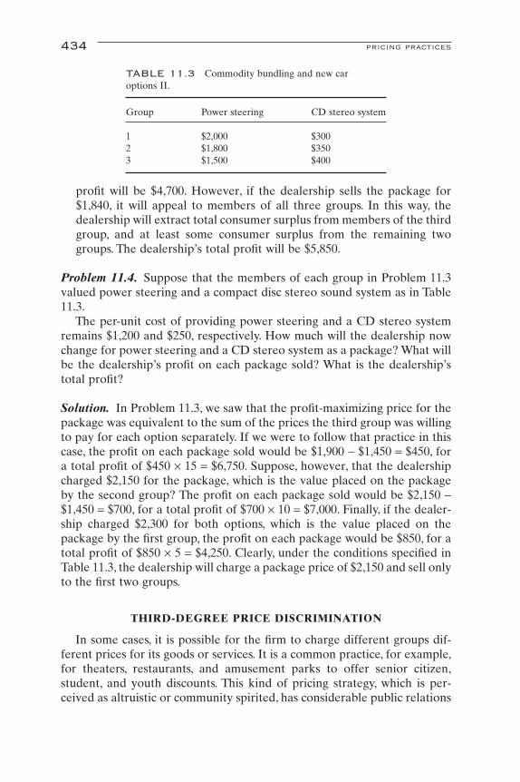
profit will be $4,700. However, if the dealership sells the package for$1,840, it will appeal to members of all three groups. In this way, the dealership will extract total consumer surplus from members of the thirdgroup, and at least some consumer surplus from the remaining twogroups. The dealership’s total profit will be $5,850.

Problem 11.4. Suppose that the members of each group in Problem 11.3valued power steering and a compact disc stereo sound system as in Table11.3.

The per-unit cost of providing power steering and a CD stereo systemremains $1,200 and $250, respectively. How much will the dealership nowchange for power steering and a CD stereo system as a package? What willbe the dealership’s profit on each package sold? What is the dealership’stotal profit?

Solution. In Problem 11.3, we saw that the profit-maximizing price for thepackage was equivalent to the sum of the prices the third group was willingto pay for each option separately. If we were to follow that practice in thiscase, the profit on each package sold would be $1,900 - $1,450 = $450, fora total profit of $450 ¥ 15 = $6,750. Suppose, however, that the dealershipcharged $2,150 for the package, which is the value placed on the packageby the second group? The profit on each package sold would be $2,150 -$1,450 = $700, for a total profit of $700 ¥ 10 = $7,000. Finally, if the dealer-ship charged $2,300 for both options, which is the value placed on thepackage by the first group, the profit on each package would be $850, for atotal profit of $850 ¥ 5 = $4,250. Clearly, under the conditions specified inTable 11.3, the dealership will charge a package price of $2,150 and sell onlyto the first two groups.

THIRD-DEGREE PRICE DISCRIMINATION

In some cases, it is possible for the firm to charge different groups dif-ferent prices for its goods or services. It is a common practice, for example,for theaters, restaurants, and amusement parks to offer senior citizen,student, and youth discounts. This kind of pricing strategy, which is per-ceived as altruistic or community spirited, has considerable public relations


TABLE 11.3 Commodity bundling and new car options II.

Group Power steering CD stereo system

1 $2,000 $3002 $1,800 $3503 $1,500 $400

appeal. In reality, however, this third-degree price discrimination in factresults in increased company profits.

Definition: Third-degree price discrimination occurs when firms segmentthe market for a particular good or service into easily identifiable groups,then charge each group a different price.

For third-degree price discrimination to be effective, a number of con-ditions must be satisfied. First, the firm must be able to estimate eachgroup’s demand function. As we will see, the degree of price variation willdepend of differences in each group’s price elasticity of demand. In general,groups with higher price elasticities of demand will be charged a lowerprice.

A second condition that must be satisfied for a firm to engage in third-degree price discrimination is that members of each group must be easilyidentifiable by some distinguishable characteristic, such as age; or perhapsgroups can be identified in terms of the time of the day in which the goodor service, such as movie tickets, is purchased.

Finally, for third-degree price discrimination to be successful, it must notbe possible for groups purchasing the good or service at a lower price to beable to resell that good or service to groups changed the higher price. Ifresales are possible, the firm would not be able to sell anything to the grouppaying the higher price because they would simply buy the good or servicefrom the group eligible for the lower price.

The rationale behind third-degree price discrimination is straightfor-ward. Different individuals or groups of individuals with different demandfunctions will have different marginal revenue functions. Since the marginalcost of producing the good is the same, regardless of which group purchasesthe good, the profit-maximizing condition must be MC = MR1 = MR2 = ◊ ◊ ◊= MRn, where n is the number of identifiable and separable groups. To seewhy this must be the case, suppose that MR1 > MC. Clearly, in this case, itwould pay for the firm to produce one more unit of the good or service andsell it to group 1, since the addition to total revenues would exceed the addi-tion to total cost from producing the good. As more of the good or serviceis sold to group 1, marginal revenue will fall until MR1 = MC is established.

The mathematics of this third-degree price discrimination is fairlystraightforward. Assume that a firm sells its product in two easily identifi-able markets. The total output of the firm is, therefore,

(11.11)

By the law of demand, the quantity sold in each market will varyinversely with the selling price. If the demand function of each group isknown, the total revenue earned by the firm selling its product in eachmarket will be

(11.12)TR Q TR Q TR Q( ) = ( ) + ( )1 1 2 2

Q Q Q= +1 2


where TR1 = P1Q1 and TR2 = P2Q2. The total cost of producing the good orservice is a function of total output, or,

(11.13)

Note that the marginal cost of producing the good is the same for bothmarkets. By the chain rule,

(11.14)

since ∂Q/∂Q1 = 1. Likewise for Q2,

(11.15)

since ∂Q/∂Q2 = 1. Equations (11.14) and (11.15) simply affirm that the mar-ginal cost of producing the good or service remains the same, regardless ofthe market in which it is sold.

Upon combining Equations (11.11) to (11.15), the firm’s profit functionmay be written

(11.16)

Equation (11.16) indicates that profit is a function of both Q1 and Q2.The objective of the firm is to maximize profit with respect to both Q1 andQ2. Taking the first partial derivatives of the profit function with respect toQ1 and Q2, and setting the results equal to zero, we obtain

(11.17a)

(11.17b)

Solving Equations (11.17) simultaneously with respect to Q1 and Q2

yields the profit-maximizing unit sales in the two markets. Assuming thatthe second-order conditions are satisfied, the first-order conditions forprofit maximization may be written as

(11.18)

Finally, since TR1 = P1Q1 and TR2 = P2Q2, then

(11.19)

MR PdQdQ

QdPdQ

PdPdQ

QP

P

1 11

11

1

1

11

1

1

11

11 1

1

= ÊË

ˆ¯ + Ê

Ëˆ¯

= + ÊË

ˆ¯ÊË

ˆ¯

ÈÎÍ

˘˚

= +ÊË

ˆ¯e

MC MR MR= =1 2

∂p∂

∂∂

∂∂Q

TRQ

dTCdQ

QQ2

2

2 20= - Ê

Ëˆ¯ÊË

ˆ¯ =

∂p∂

∂∂

∂∂Q

TRQ

dTCdQ

QQ1

1

1 10= - Ê

Ëˆ¯ÊË

ˆ¯ =

p Q Q TR Q TR Q TC Q Q1 2 1 1 2 2 1 2,( ) = ( ) + ( ) - +( )

∂∂

∂∂

∂TC QQ

dTCdQ

QQ

TCdQ

( )= Ê

Ëˆ¯ÊË

ˆ¯ =

2 2

∂∂

∂∂

∂TC QQ

dTCdQ

QQ

TCdQ

( )= Ê

Ëˆ¯ÊË

ˆ¯ =

1 1

TC Q TC Q Q( ) = +( )1 2


(11.20)

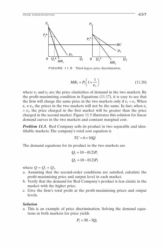
where e1 and e2 are the price elasticities of demand in the two markets. Bythe profit-maximizing condition in Equations (11.17), it is easy to see thatthe firm will charge the same price in the two markets only if e1 = e2. Whene1 π e2, the prices in the two markets will not be the same. In fact, when e1

> e2, the price charged in the first market will be greater than the pricecharged in the second market. Figure 11.5 illustrates this solution for lineardemand curves in the two markets and constant marginal cost.

Problem 11.5. Red Company sells its product in two separable and iden-tifiable markets. The company’s total cost equation is

The demand equations for its product in the two markets are

where Q = Q1 + Q2.a. Assuming that the second-order conditions are satisfied, calculate the

profit-maximizing price and output level in each market.b. Verify that the demand for Red Company’s product is less elastic in the

market with the higher price.c. Give the firm’s total profit at the profit-maximizing prices and output

levels.

Solutiona. This is an example of price discrimination. Solving the demand equa-

tions in both markets for price yields

P Q1 150 5= -

Q P2 210 0 2= - ( ).

Q P1 110 0 2= - ( ).

TC Q= +6 10

MR P2 22

11

= +ÊË

ˆ¯e


FIGURE 11.5 Third-degree price discrimination.

The corresponding total revenue equations are

Red Company’s total profit equation is

Maximizing this expression with respect to Q1 and Q2 yields

b. The relationships between the selling price and the price elasticity ofdemand in the two markets are

where

From the demand equations, dQ1/dP1 = -0.2 and dQ2/dP2 = -0.5. Substi-tuting these results into preceding above relationships, we obtain

e1 0 2304

64

1 5= -( )ÊËˆ¯ =

-= -. .

e22

2

2

2= Ê

Ëˆ¯ÊË

ˆ¯

dQdP

PQ

e11

1

1

1= Ê

Ëˆ¯ÊË

ˆ¯

dQdP

PQ

MR P2 22

11

= +ÊË

ˆ¯e

MR P1 11

11

= +ÊË

ˆ¯e

P2 30 2 5 30 10 20* = - ( ) = - =

P1 50 5 4 50 20 30* = - ( ) = - =

Q2 5* =

∂p∂Q

Q Q2

2 230 4 10 20 4 0= - - = - =

Q1 4* =

∂p∂Q

Q Q1

1 150 10 10 40 10 0= - - = - =

p = + - = - + - - - +( )TR TR TC Q Q Q Q Q Q1 2 1 12

2 22

1 250 5 30 2 6 10

TR Q Q2 2 2230 2= -

TR Q Q1 1 1250 5= -

P Q2 230 2= -


This verifies that the higher price is charged in the market where theprice elasticity of demand is less elastic.

c. The firm’s total profit at the profit-maximizing prices and output levelsare

Problem 11.6. Copperline Mountain is a world-famous ski resort in Utah.Copperline Resorts operates the resort’s ski-lift and grooming operations.When weather conditions are favorable, Copperline’s total operating cost,which depends on the number of skiers who use the facilities each year, isgiven as

where S is the total number of skiers (in hundreds of thousands). The man-agement of Copperline Resorts has determined that the demand for ski-lifttickets can be segmented into adult (SA) and children 12 years old andunder (SC). The demand curve for each group is given as

where PA and PC are the prices charged for adults and children, respectively.a. Assuming that Copperline Resorts is a profit maximizer, how many

skiers will visit Copperline Mountain?b. What prices should the company charge for adult and child’s ski-lift

tickets?c. Assuming that the second-order conditions for profit maximization are

satisfied, what is Copperline’s total profit?

Solutiona. Total profit is given by the expression

Taking the first partial derivatives with respect to SA and SC, setting theresults equal to zero, and solving, we write

p = - = +( ) -= + -= -( ) + -( ) - +( ) +[ ]= - + + - -

TR TC TR TR TC

P S P S TC

S S S S S S

S S S SC

A

A A

A A A

A A

C

C C

C C C

C

50 5 30 2 10 6

6 40 20 5 22 2

S PC C= -15 0 5.

S PA A= -10 0 2.

TC S= +10 6

p* = ( ) - ( ) + ( ) - ( ) - - +( )= - + - - - =

50 4 5 4 30 5 2 5 6 10 4 5

200 80 150 50 6 90 124

2 2

e2 0 5205

105

2= -( )ÊËˆ¯ =

-= -.


The total number of skiers that will visit Copperline Mountain is

b. Substituting these results into the demand functions yields adult andchild’s, ski-lift ticket prices.

c. Substituting the results from part a into the total profit equation yields

Problem 11.7. Suppose that a firm sells its product in two separablemarkets. The demand equations are

The firm’s total cost equation is

a. If the firm engages in third-degree price discrimination, how muchshould it sell, and what price should it charge, in each market?

b. What is the firm’s total profit?

Solutiona. Assuming that the firm is a profit maximizer, set MR = MC in each

market to determine the output sold and the price charged. Solving thedemand equation for P in each market yields

TC Q Q= + +150 5 0 5 2.

Q P2 250 0 25= - .

Q P1 1100= -

p = - + ( ) + ( ) - ( ) - ( )= - + + - - = ¥( )

6 40 4 20 5 5 4 2 5

6 160 100 80 50 124 10

2 2

3$

PC = $20

5 15 0 5= - . PC

PA = $30

4 10 0 2= - . PA

S S S= = = + = ¥( )A C skiers4 5 9 105

SC = 5

∂p∂S

SC

C= - =20 4 0

SA = 4

∂p∂S

SA

A= - =40 10 0


The respective total and marginal revenue equations are

The firm’s marginal cost equation is

Setting MR = MC for each market yields

b. The firm’s total profit is

Problem 11.8. Suppose that the firm in Problem 11.7 charges a uniformprice in the two markets in which it sells its product.a. Find the uniform price charged, and the quantity sold, in the two

markets.b. What is the firm’s total profit?c. Compare your answers to those obtained in Problem 11.7.

Solutiona. To determine the uniform price charged in each market, first add the two

demand equations:

p* .

. . . , . $ , .

= + - + +( ) + +( )ÈÎÍ

˘˚

= ( ) + ( ) - + +( ) =

P Q P Q Q Q Q Q1 1 2 2 1 2 1 2

2

150 5 0 5

68 33 31 67 140 15 150 233 35 1 089 04 2 791 62

* * * * * * * *

P2 200 4 15 140 00* $ .= - ( ) =

P1 100 31 67 68 33* . $ .= - =

Q2 15* =

Q1 31 67* = .

200 8 52 2- = +Q Q

100 2 51 1- = +Q Q

MCdTCdQ

Q= = +5

MR Q2 2200 8= -

MR Q1 1100 2= -

TR Q Q2 2 22200= -

TR Q Q1 1 12100= -

P Q2 2200 4= -

P Q1 1100= -


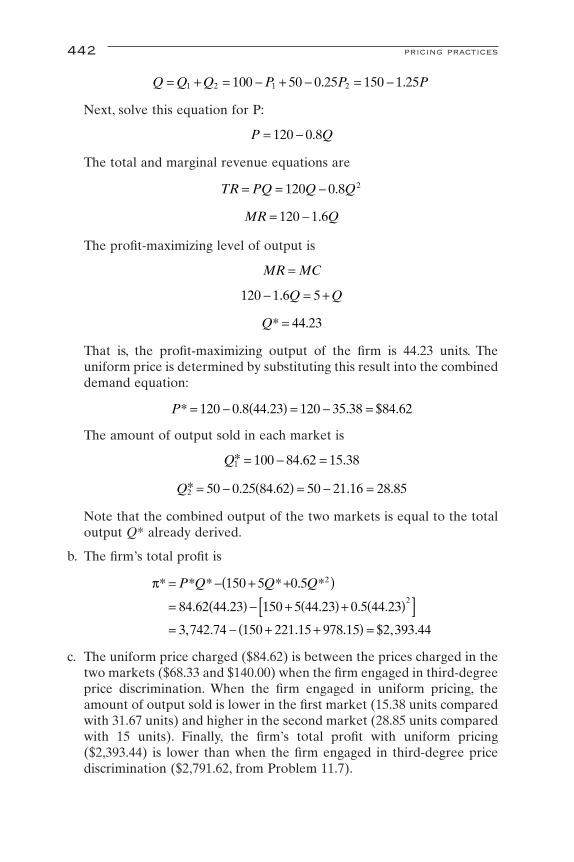
Next, solve this equation for P:

The total and marginal revenue equations are

The profit-maximizing level of output is

That is, the profit-maximizing output of the firm is 44.23 units. Theuniform price is determined by substituting this result into the combineddemand equation:

The amount of output sold in each market is

Note that the combined output of the two markets is equal to the totaloutput Q* already derived.


c. The uniform price charged ($84.62) is between the prices charged in thetwo markets ($68.33 and $140.00) when the firm engaged in third-degreeprice discrimination. When the firm engaged in uniform pricing, theamount of output sold is lower in the first market (15.38 units comparedwith 31.67 units) and higher in the second market (28.85 units comparedwith 15 units). Finally, the firm’s total profit with uniform pricing($2,393.44) is lower than when the firm engaged in third-degree pricediscrimination ($2,791.62, from Problem 11.7).

p* * * * . *

. . . . .

, . . . $ , .

= - + +( )= ( ) - + ( ) + ( )[ ]= - + +( ) =

P Q Q Q150 5 0 5

84 62 44 23 150 5 44 23 0 5 44 23

3 742 74 150 221 15 978 15 2 393 44

2

2

Q2 50 0 25 84 62 50 21 16 28 85* . . . .= - ( ) = - =

Q1 100 84 62 15 38* . .= - =

P* . . . $ .= - ( ) = - =120 0 8 44 23 120 35 38 84 62

Q* .= 44 23

120 1 6 5- = +. Q Q

MR MC=

MR Q= -120 1 6.

TR PQ Q Q= = -120 0 8 2.

P Q= -120 0 8.

Q Q Q P P P= + = - + - = -1 2 1 2100 50 0 25 150 1 25. .


When third-degree price discrimination is practiced in foreign trade it issometimes referred to as dumping. This rather derogatory term is oftenused by domestic producers claiming unfair foreign competition. Definedby the U.S. Department of Commerce as selling at below fair market value,dumping results when a profit-maximizing exporter sells its product at a dif-ferent, usually lower, price in the foreign market than it does in its homemarket. Recall that when resale between two markets is not possible, themonopolist will sell its product at a lower price in the market in whichdemand is more price elastic. In international trade theory, the differencebetween the home price and the foreign price is called the dumping margin.

NONMARGINAL PRICING

Most of the discussion of pricing practices thus far has assumed that man-agement is attempting to optimize some corporate objective. For the mostpart, we have assumed that management attempts to maximize the firm’sprofits, but other optimizing behavior has been discussed, such as revenuemaximization. In each case, we assumed that the firm was able to calculateits total cost and total revenue equations, and to systematically use thatinformation to achieve the firm’s objectives. If the firm’s objective is to maximize profit, for example, then management will produce at an outputlevel and charge a price at which marginal revenue equals marginal cost.This is the classic example of marginal pricing.

In reality, however, firms do not know their total revenue and total costequations, nor are they ever likely to. In fact, because firms do not have thisinformation, and in spite management’s protestations to the contrary, mostfirms are (unwittingly) not profit maximizers. Moreover, even if this infor-mation were available, there are other corporate objectives, such as satis-ficing behavior, that do not readily lend themselves to marginal pricingstrategies. Consequently, most firms engage in nonmarginal pricing. Themost popular form of nonmarginal pricing is cost-plus pricing.

Definition: Firms determine the profit-maximizing price and output levelby equating marginal revenue with marginal cost. When the firm’s totalrevenue and total cost equations are unknown, however, management willoften practice nonmarginal pricing. The most popular form of nonmarginalpricing is cost-plus pricing, also known as markup or full-cost pricing.

COST-PLUS PRICING

As we have seen, profit maximization occurs at the price–quantity com-bination at which where marginal cost equals marginal revenue. In reality,however, many firms are unable or unwilling to devote the resources nec-essary to accurately estimate the total revenue and total cost equations, or

nonmarginal pricing 443

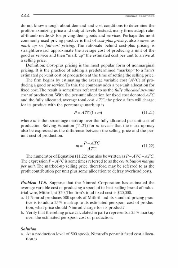
do not know enough about demand and cost conditions to determine theprofit-maximizing price and output levels. Instead, many firms adopt rule-of-thumb methods for pricing their goods and services. Perhaps the mostcommonly used pricing practice is that of cost-plus pricing, also known asmark up or full-cost pricing. The rationale behind cost-plus pricing isstraightforward: approximate the average cost of producing a unit of thegood or service and then “mark up” the estimated cost per unit to arrive ata selling price.

Definition: Cost-plus pricing is the most popular form of nonmarginalpricing. It is the practice of adding a predetermined “markup” to a firm’sestimated per-unit cost of production at the time of setting the selling price.

The firm begins by estimating the average variable cost (AVC) of pro-ducing a good or service. To this, the company adds a per-unit allocation forfixed cost. The result is sometimes referred to as the fully allocated per-unitcost of production. With the per-unit allocation for fixed cost denoted AFCand the fully allocated, average total cost ATC, the price a firm will chargefor its product with the percentage mark up is

(11.21)

where m is the percentage markup over the fully allocated per-unit cost ofproduction. Solving Equation (11.21) for m reveals that the mark up mayalso be expressed as the difference between the selling price and the per-unit cost of production.

(11.22)

The numerator of Equation (11.22) can also be written as P - AVC - AFC.The expression P - AVC is sometimes referred to as the contribution marginper unit. The marked-up selling price, therefore, may be referred to as theprofit contribution per unit plus some allocation to defray overhead costs.

Problem 11.9. Suppose that the Nimrod Corporation has estimated theaverage variable cost of producing a spool of its best-selling brand of indus-trial wire, Mithril, at $20. The firm’s total fixed cost is $20,000.a. If Nimrod produces 500 spools of Mithril and its standard pricing prac-

tice is to add a 25% markup to its estimated per-spool cost of produc-tion, what price should Nimrod charge for its product?

b. Verify that the selling price calculated in part a represents a 25% markupover the estimated per-spool cost of production.

Solutiona. At a production level of 500 spools, Nimrod’s per-unit fixed cost alloca-

tion is

mP ATC

ATC=

-

P ATC m= +( )1


The cost-plus pricing equation is given as

where m is the percentage markup and ATC is the sum of the averagevariable cost of production (AVC) and the per-unit fixed cost allocation(AFC). Substituting, we write

Nimrod should charge $75 per spool of Mithril. In other words, Nimrodshould charge $15 over its estimated per-unit cost of production.

b. The percentage markup is given by the equation

Substituting the relevant data into this equation yields

Of course, the advantage of cost-plus pricing is its simplicity. Cost-pluspricing requires less than complete information, and it is easy to use. Caremust be exercised, however, when one is using this approach. The useful-ness of cost-plus pricing will be significantly reduced unless the appropri-ate cost concepts are employed. As in the case of break-even analysis, caremust be taken to include all relevant costs of production. Cost-plus pricing,which is based only on accounting (explicit) costs, will move the firm furtheraway from an optimal (profit-maximizing) price and output level. Of course,the more appropriate approach would be to calculate total economic costs,which include both explicit and implicit costs of production.

There are two major criticisms of cost-plus pricing. The first criticisminvolves the assumption of fixed marginal cost, which at fixed input pricesis in defiance of the law of diminishing marginal product. It is this assump-tion that allows us to further assume that marginal cost is approximatelyequal to the fully allocated per-unit cost of production. If it can be argued,however, that marginal cost is approximately constant over the firm’s rangeof production, this criticism loses much of its sting.

A perhaps more serious criticism of cost-plus pricing is that it is insen-sitive to demand conditions. It should be noted that, in practice, the size ofa firm’s markup tends to reflect the price elasticity of demand for of goodsof various types. Where the demand for a product is relatively less priceelastic, because of, say, the paucity of close substitutes, the markup tends to

m =-

= =75 60

601560

0 25.

mP ATC

ATC=

-( )

P = +( ) +( ) = ( ) =20 40 1 0 25 60 1 25 75. . $

P ATC m= +( )1

AFC = =20 000

50040

,


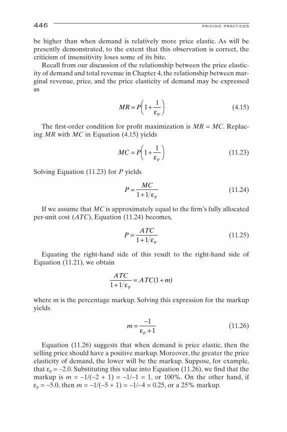
be higher than when demand is relatively more price elastic. As will bepresently demonstrated, to the extent that this observation is correct, thecriticism of insensitivity loses some of its bite.

Recall from our discussion of the relationship between the price elastic-ity of demand and total revenue in Chapter 4, the relationship between mar-ginal revenue, price, and the price elasticity of demand may be expressedas

(4.15)

The first-order condition for profit maximization is MR = MC. Replac-ing MR with MC in Equation (4.15) yields

(11.23)

Solving Equation (11.23) for P yields

(11.24)

If we assume that MC is approximately equal to the firm’s fully allocatedper-unit cost (ATC), Equation (11.24) becomes,

(11.25)

Equating the right-hand side of this result to the right-hand side of Equation (11.21), we obtain

where m is the percentage markup. Solving this expression for the markupyields

(11.26)

Equation (11.26) suggests that when demand is price elastic, then theselling price should have a positive markup. Moreover, the greater the priceelasticity of demand, the lower will be the markup. Suppose, for example,that ep = -2.0. Substituting this value into Equation (11.26), we find that themarkup is m = -1/(-2 + 1) = -1/-1 = 1, or 100%. On the other hand, if ep = -5.0, then m = -1/(-5 + 1) = -1/-4 = 0.25, or a 25% markup.

m =-+1

1ep

ATCATC m

1 11

+= +( )

ep

PATC

=+1 1 ep

PMC

=+1 1 ep

MC P= +ÊË

ˆ¯1

1ep

MR P= +ÊË

ˆ¯1

1ep


What happens, however, if the demand for the good or service is priceinelastic? Suppose, for example, that ep = -0.8. Substituting this into Equa-tion (11.26) results in a markup of m = -1/(-0.8 + 1) = -1/0.2 = -5.This resultsuggests that the firm should mark down the price of its product by 500%!Equation (11.26) suggests that if the demand for a product is price inelas-tic, the firm should sell its output at below the fully allocated per-unit costof production, a practice that is clearly not observed in the real world.Fortunately, this apparent paradox is easily resolved.

It will be recalled from Chapter 4, and is easily seen from Equation(4.15), that when the demand for a good or service is price inelastic, it mar-ginal revenue must be negative. For the profit-maximizing firm, this sug-gests that marginal cost is negative, since the first-order condition for profitmaximization is MR = MC, which is clearly impossible for positive inputprices and positive marginal product of factors of production.

Problem 11.10. What is the estimated percentage markup over the fullyallocated per-unit cost of production for the following price elasticities ofdemand?a. ep = -11b. ep = -4c. ep = -2.5d. ep = -2.0e. ep = -1.5

Solution

a. or a 10% mark up

b. or a 33.3% mark up

c. or a 66.7% mark up

d. or a 100% mark up

e. or a 200% mark up

Problem 11.11. What is the percentage markup on the output of a firmoperating in a perfectly competitive industry?

Solution. A firm operating in a perfectly competitive industry faces an infi-nitely elastic demand for its product. Substituting ep = -• into Equation(11.26) yields

m =-+

=-

- +=

11

11 5 1

2 0ep .

.

m =-+

=-

- +=

11

12 0 1

1 0ep .

.

m =-+

=-

- +=

11

12 5 1

0 667ep .

.

m =-+

=-

- +=

11

14 1

0 333ep

.

m =-+

=-

- +=

11

111 1

0 10ep

.


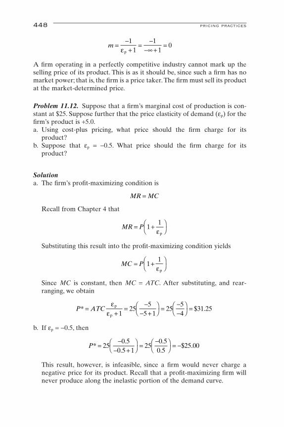
A firm operating in a perfectly competitive industry cannot mark up theselling price of its product. This is as it should be, since such a firm has nomarket power; that is, the firm is a price taker. The firm must sell its productat the market-determined price.

Problem 11.12. Suppose that a firm’s marginal cost of production is con-stant at $25. Suppose further that the price elasticity of demand (ep) for thefirm’s product is +5.0.a. Using cost-plus pricing, what price should the firm charge for its

product?b. Suppose that ep = -0.5. What price should the firm charge for its

product?

Solutiona. The firm’s profit-maximizing condition is

Recall from Chapter 4 that

Substituting this result into the profit-maximizing condition yields

Since MC is constant, then MC = ATC. After substituting, and rear-ranging, we obtain

b. If ep = -0.5, then

This result, however, is infeasible, since a firm would never charge a negative price for its product. Recall that a profit-maximizing firm willnever produce along the inelastic portion of the demand curve.

P*.

..

.$ .=

-- +

ÊË

ˆ¯ =

-ÊË

ˆ¯ = -25

0 50 5 1

250 5

0 525 00

P ATC* $ .=+

=-

- +ÊË

ˆ¯ =

--

ÊË

ˆ¯ =

ee

p

p 125

55 1

2554

31 25

MC P= +ÊË

ˆ¯1

1ep

MR P= +ÊË

ˆ¯1

1ep

MR MC=

m =-+

=-

-• +=

11

11

0ep


MULTIPRODUCT PRICING

We have thus far considered primarily firms that produce and sell onlyone good or service at a single price. The only exception to this generalstatement was our discussion of commodity bundling, in which a firm sellsa package of goods at a single price.We will now address the issue of pricingstrategies of a single firm selling more than one product under alternativescenarios. These scenarios include the optimal pricing of two or more products with interdependent demands, optimal pricing of two or moreproducts with independent demands that are jointly produced in variableproportions, and optimal pricing of two or more products with independentdemands that are jointly produced in fixed proportions.

Definition: Multiproduct pricing involves optimal pricing strategies offirms producing and selling more than one good or service.

OPTIMAL PRICING OF TWO OR MORE PRODUCTSWITH INTERDEPENDENT DEMANDS AND

INDEPENDENT PRODUCTION

Often a firm will produce two or more goods that are either comple-ments or substitutes for each other. Dell Computer, for example, sells anumber of different models of personal computers. These models are, to a degree, substitutes for each other. Personal computers also come with avariety of accessories (mouses, printers, modems, scanners, etc.). Theseoptions not only come in different models, and are, therefore, substitutesfor each other, but they are also complements to the personal computers.

Because of the interrelationships inherent in the production of somegoods and services, it stands to reason that an increase in the price of, say,a Dell personal computer model will lead to a reduction in the quantitydemanded of that model and an increase in the demand for substitutemodels. Moreover, an increase in the price of the Dell personal computermodel will lead to a reduction in the demand for complementary acces-sories. For this reason, a profit-maximizing firm must ascertain the optimalprices and output levels of each product manufactured jointly, rather thanpricing each product independently.

The problem may be formally stated as follows. Consider the demandfor two products produced by the same firm. If these two products arerelated, the demand functions may be expressed as

(11.27a)

(11.27b)

By the law of demand, ∂Q1/∂P1 and ∂Q2/∂P2 are negative. The signs of∂Q1/∂Q2 and ∂Q2/∂Q1 depend on the relationship between Q1 and Q2. If the

Q f P Q2 2 2 1= ( ),

Q f P Q1 1 1 2= ( ),

multiproduct pricing 449

values of these first partial derivatives are positive, then Q1 and Q2 are com-plements. If the values of these first partials are negative, then Q1 and Q2

are substitutes.Upon solving Equation (11.27a) for P1 and Equation (11.27b) for P2, and

substituting these results into the total revenue equations, we write

(11.28a)

(11.28b)

Since the two goods are independently produced, the total cost functionsare

(11.29a)

(11.29b)

The total profit equation for this firm is, therefore,

(11.30)

The first-order conditions for profit maximization are

(11.31a)

(11.31b)

which may be expressed as

(11.32a)

(11.32b)

We will assume that the second-order conditions for profit maximizationare satisfied.

Equations (11.32) indicate that a firm producing two products with inter-related demands will maximize its profits by producing where marginal costis equal to the change in total revenue derived from the sale of the productitself, plus the change in total revenue derived from the sale of the relatedproduct. If the second term on the right-hand side of Equation (11.31) is

MCTRQ

TRQ2

2

2

1

2= +

∂∂

∂∂

MCTRQ

TRQ1

1

1

2

1= +

∂∂

∂∂

∂p∂

∂∂

∂∂

∂∂Q

TRQ

TRQ

TCQ2

2

2

1

2

2

20= + - =

∂p∂

∂∂

∂∂

∂∂Q

TRQ

TRQ

TCQ1

1

1

2

1

1

10= + - =

p = ( ) + ( ) - ( ) - ( )= + + ( ) - ( )= ( ) + ( ) - ( ) - ( )

TR Q Q TR Q Q TC Q TC Q

P Q P Q TC Q TC Q

h Q Q Q h Q Q Q TC Q TC Q

1 1 2 2 1 2 1 1 2 2

1 1 2 2 1 1 2 2

1 1 2 1 2 1 2 2 1 1 2 2

, ,

, ,

TC TC Q2 2 2= ( )

TC TC Q1 1 1= ( )

TR Q Q P Q h Q Q Q2 1 2 2 2 2 1 2 2, ,( ) = = ( )

TR Q Q P Q h Q Q Q1 1 2 1 1 1 1 2 1, ,( ) = = ( )


positive, then Q1 and Q2 are complements. If this term is negative, then Q1

and Q2 are substitutes.

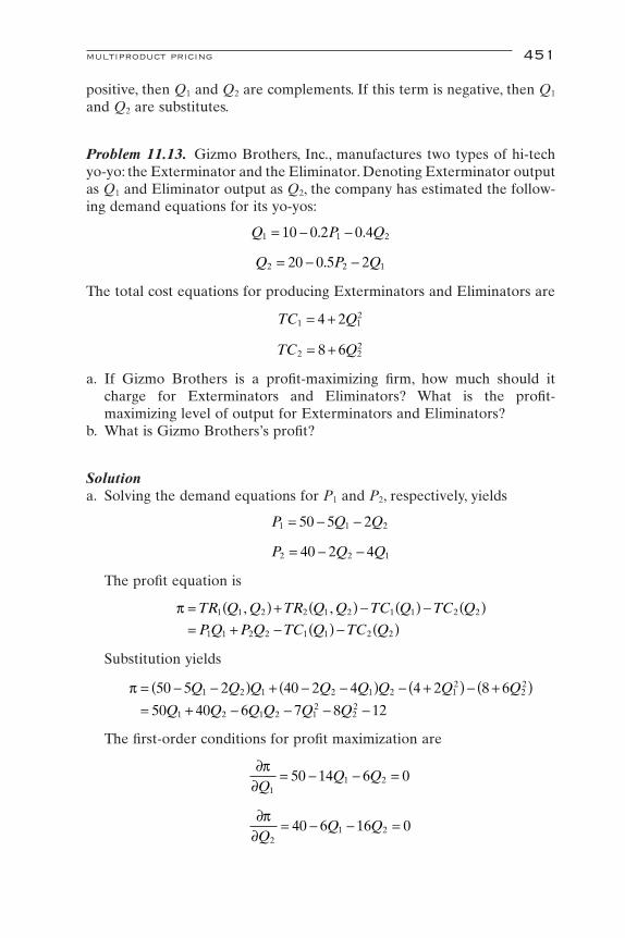
Problem 11.13. Gizmo Brothers, Inc., manufactures two types of hi-techyo-yo: the Exterminator and the Eliminator. Denoting Exterminator outputas Q1 and Eliminator output as Q2, the company has estimated the follow-ing demand equations for its yo-yos:

The total cost equations for producing Exterminators and Eliminators are

a. If Gizmo Brothers is a profit-maximizing firm, how much should itcharge for Exterminators and Eliminators? What is the profit-maximizing level of output for Exterminators and Eliminators?

b. What is Gizmo Brothers’s profit?

Solutiona. Solving the demand equations for P1 and P2, respectively, yields

The profit equation is

Substitution yields


∂p∂Q

Q Q2

1 240 6 16 0= - - =

∂p∂Q

Q Q1

1 250 14 6 0= - - =

p = - -( ) + - -( ) - +( ) - +( )= + - - - -

50 5 2 40 2 4 4 2 8 6

50 40 6 7 8 121 2 1 2 1 2 1

222

1 2 1 2 12

22

Q Q Q Q Q Q Q Q

Q Q Q Q Q Q

p = ( ) + ( ) - ( ) - ( )= + - ( ) - ( )

TR Q Q TR Q Q TC Q TC Q

P Q P Q TC Q TC Q1 1 2 2 1 2 1 1 2 2

1 1 2 2 1 1 2 2

, ,

P Q Q2 2 140 2 4= - -

P Q Q1 1 250 5 2= - -

TC Q2 228 6= +

TC Q1 124 2= +

Q P Q2 2 120 0 5 2= - -.

Q P Q1 1 210 0 2 0 4= - -. .


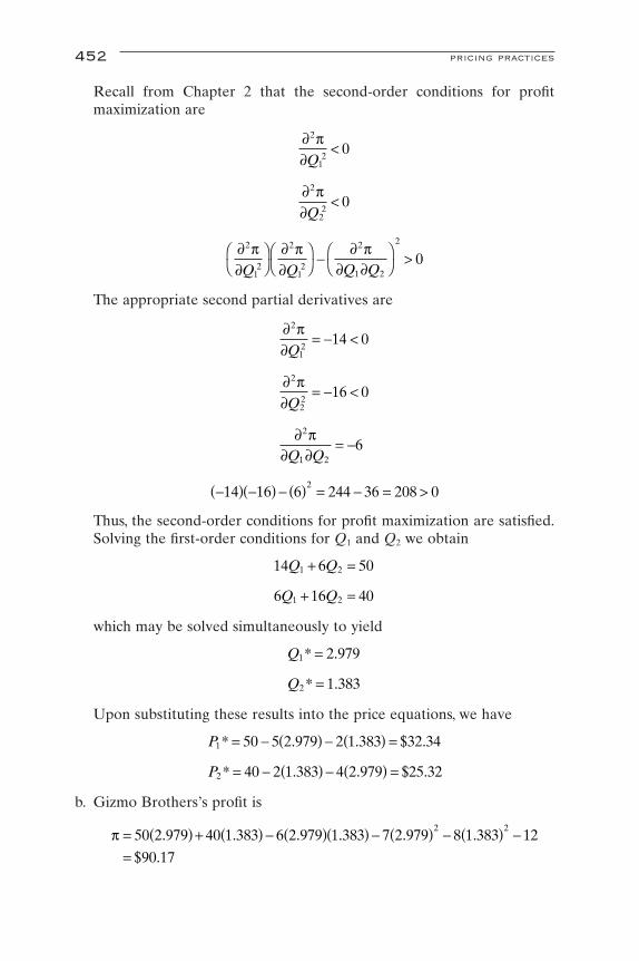
Recall from Chapter 2 that the second-order conditions for profit maximization are

The appropriate second partial derivatives are

Thus, the second-order conditions for profit maximization are satisfied.Solving the first-order conditions for Q1 and Q2 we obtain

which may be solved simultaneously to yield

Upon substituting these results into the price equations, we have

b. Gizmo Brothers’s profit is

p = ( ) + ( ) - ( )( ) - ( ) - ( ) -=

50 2 979 40 1 383 6 2 979 1 383 7 2 979 8 1 383 12

90 17

2 2. . . . . .

$ .

P2 40 2 1 383 4 2 979 25 32* . . $ .= - ( ) - ( ) =

P1 50 5 2 979 2 1 383 32 34* . . $ .= - ( ) - ( ) =

Q2 1 383* .=

Q1 2 979* .=

6 16 401 2Q Q+ =

14 6 501 2Q Q+ =

-( ) -( ) - ( ) = - = >14 16 6 244 36 208 02

∂ p∂ ∂

2

1 26

Q Q= -

∂ p∂

2

22

16 0Q

= - <

∂ p∂

2

12

14 0Q

= - <

∂ p∂

∂ p∂

∂ p∂ ∂

2

12

2

12

2

1 2

2

0Q Q Q Q

ÊË

ˆ¯ÊË

ˆ¯ - Ê

Ëˆ¯ >

∂ p∂

2

22

0Q

<

∂ p∂

2

12

0Q

<


OPTIMAL PRICING OF TWO OR MORE PRODUCTSWITH INDEPENDENT DEMANDS JOINTLYPRODUCED IN VARIABLE PROPORTIONS

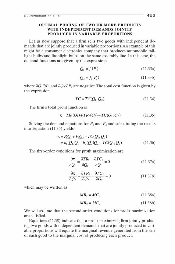
Let us now suppose that a firm sells two goods with independent de-mands that are jointly produced in variable proportions.An example of thismight be a consumer electronics company that produces automobile tail-light bulbs and flashlight bulbs on the same assembly line. In this case, thedemand functions are given by the expressions

(11.33a)

(11.33b)

where ∂Q1/∂P1 and ∂Q2/∂P2 are negative. The total cost function is given bythe expression

(11.34)

The firm’s total profit function is

(11.35)

Solving the demand equations for P1 and P2 and substituting the resultsinto Equation (11.35) yields

(11.36)


(11.37a)

(11.37b)

which may be written as

(11.38a)

(11.38b)

We will assume that the second-order conditions for profit maximizationare satisfied.

Equations (11.38) indicate that a profit-maximizing firm jointly produc-ing two goods with independent demands that are jointly produced in vari-able proportions will equate the marginal revenue generated from the saleof each good to the marginal cost of producing each product.

MR MC2 2=

MR MC1 1=

∂p∂

∂∂

∂∂Q

TRQ

TCQ2

2

2

2

20= - =

∂p∂

∂∂

∂∂Q

TRQ

TCQ1

1

1

1

10= - =

p = + - ( )= ( ) + ( ) - ( )

P Q P Q TC Q Q

h Q Q h Q Q TC Q Q1 1 2 2 1 2

1 1 1 2 2 2 1 2

,

,

p = ( ) + ( ) - ( )TR Q TR Q TC Q Q1 1 2 2 1 2,

TC TC Q Q= ( )1 2,

Q f P2 2 2= ( )

Q f P1 1 1= ( )


Problem 11.14. Suppose Gizmo Brothers also produces Tommy Gunnaction figures for boys ages 7 to 12, and Bonzey, a toy bone for pet dogs.Except for the molding phase, both products are made on the same assem-bly line. Denoting Tommy Gunn as Q1 and Bonzey as Q2, the company hasestimated the following demand equations:

The total cost equation for producing the two products is

a. As before, Gizmo Brothers is a profit-maximizing firm. Give the profit-maximizing levels of output for Tommy Gunn and for Bonzey. Howmuch should the firm charge for Tommy Gunn and Bonzey?

b. What is Gizmo Brothers’s profit?

Solutiona. Solving the demand equations for P1 and P2, respectively, yields

Gizmo Brothers’s profit equation is

Substituting the demand equations into the profit equation yield


The second-order conditions for profit maximization are

∂p∂Q

Q Q2

2 1100 16 2 0= - - =

∂p∂Q

Q Q1

1 220 6 2 0= - - =

p = -( ) + -( ) - + + +( )= - + + - - -

20 2 100 5 2 3 10

10 20 100 3 8 21 1 2 2 1

21 2 2

2

1 2 12

22

1 2

Q Q Q Q Q Q Q Q

Q Q Q Q Q Q

p = ( ) + ( ) - ( ) = + - ( )TR Q TR Q TC Q Q P Q P Q TC Q Q1 1 2 2 1 1 2 1 1 2 2 1 1 2, ,

P Q2 2100 5= -

P Q1 120 2= -

TC Q Q Q Q= + + +12

1 2 222 3 10

Q P2 220 0 2= - .

Q P1 110 0 5= - .


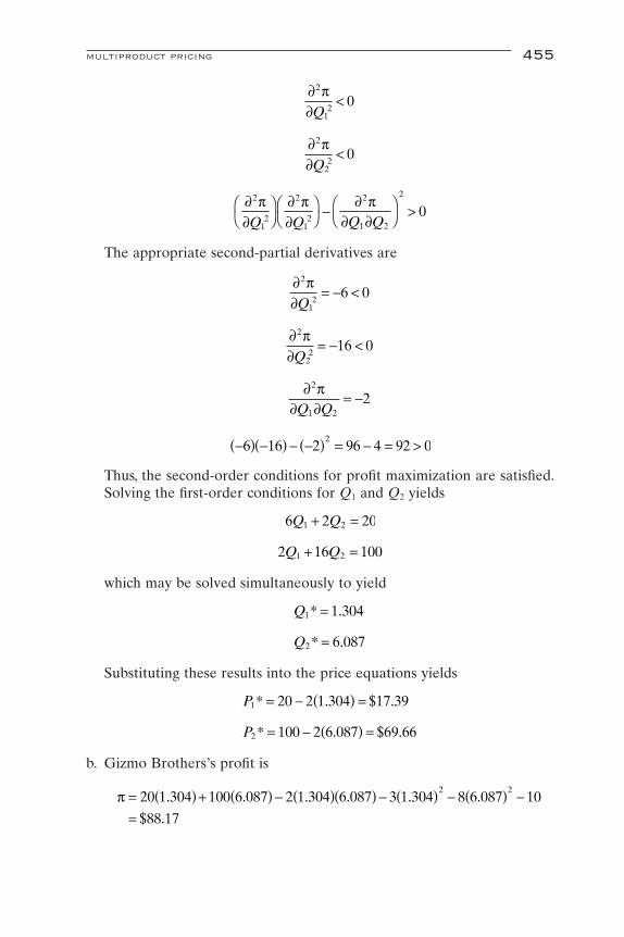
The appropriate second-partial derivatives are

Thus, the second-order conditions for profit maximization are satisfied.Solving the first-order conditions for Q1 and Q2 yields

which may be solved simultaneously to yield

Substituting these results into the price equations yields

b. Gizmo Brothers’s profit is

p = ( ) + ( ) - ( )( ) - ( ) - ( ) -=

20 1 304 100 6 087 2 1 304 6 087 3 1 304 8 6 087 10

88 17

2 2. . . . . .

$ .

P2 100 2 6 087 69 66* . $ .= - ( ) =

P1 20 2 1 304 17 39* . $ .= - ( ) =

Q2 6 087* .=

Q1 1 304* .=

2 16 1001 2Q Q+ =

6 2 201 2Q Q+ =

-( ) -( ) - -( ) = - = >6 16 2 96 4 92 02

∂ p∂ ∂

2

1 22

Q Q= -

∂ p∂

2

22

16 0Q

= - <

∂ p∂

2

12

6 0Q

= - <

∂ p∂

∂ p∂

∂ p∂ ∂

2

12

2

12

2

1 2

2

0Q Q Q Q

ÊË

ˆ¯ÊË

ˆ¯ - Ê

Ëˆ¯ >

∂ p∂

2

22

0Q

<

∂ p∂

2

12

0Q

<


OPTIMAL PRICING OF TWO OR MORE PRODUCTSWITH INDEPENDENT DEMANDS JOINTLY

PRODUCED IN FIXED PROPORTIONS

Now, let us assume that a firm jointly produces two goods in fixed pro-portions but with independent demands. In many cases, the second productis a by-product of the first, such as beef and hides. With joint production infixed proportions, it is conceptually impossible to consider two separateproducts, since the production of one good automatically determines thequantity produced of the other.

Suppose that the demand functions for two goods produced jointly aregiven as Equations (11.33). The total cost equation is given as Equation(11.13).

(11.13)

The analysis differs, however, in that Q1 and Q2 are in direct proportion toeach other, that is,

(11.39)

where the constant k > 0. Solving Equation (11.33) for P1 and P2 yields

(11.40a)

(11.40b)

Substituting Equation (11.39) into Equations (11.13) and (11.40b) yields

(11.41)

(11.42)

Substituting Equations (11.39), (11.40a), (11.41), and (11.42) into Equa-tion (11.36) yields the firm’s profit equation:

(11.43)

Stated another way, the firm’s total profit function is

(11.44)

Equation (11.44) indicates that total profit is a function of the single deci-sion variable, Q1. Equation (11.44) may also be written

(11.45)p Q TR Q TR Q TC Q2 1 2 2 2 2( ) = ( ) + ( ) - ( )

p Q TR Q TR Q TC Q1 1 1 2 1 1( ) = ( ) + ( ) - ( )

p = + ( ) - ( )= ( ) + ( )( ) - ( )

P Q P kQ TC Q

h Q Q h Q kQ TC Q1 1 2 1 1

1 1 1 2 1 1 1

TC Q TC Q( ) = ( )1

P h Q2 2 1= ( )

P h Q1 1 1= ( )

P h Q2 2 2= ( )

P h Q1 1 1= ( )

Q kQ2 1=

TC Q TC Q Q( ) = +( )1 2


From Equation (11.44), the first-order condition for profit maximizationis

(11.46)

Equation (11.46) may be rewritten

(11.47)

Equation (11.47) says that a profit-maximizing firm that jointly producestwo goods in fixed proportions with independent demands will equate thesum of the marginal revenues of both products expressed in terms of oneof the products with the marginal cost of jointly producing both productsexpressed in terms of the same product. This situation is depicted dia-grammatically in Figure 11.6.

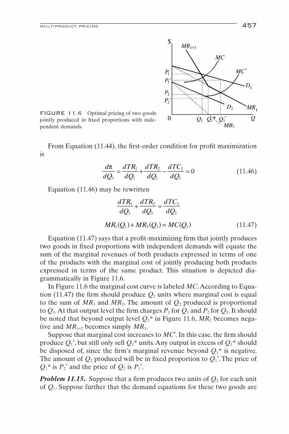
In Figure 11.6 the marginal cost curve is labeled MC.According to Equa-tion (11.47) the firm should produce Q1 units where marginal cost is equalto the sum of MR1 and MR2. The amount of Q2 produced is proportionalto Q1.At that output level the firm charges P1 for Q1 and P2 for Q2. It shouldbe noted that beyond output level Q1* in Figure 11.6, MR2 becomes nega-tive and MR1+2 becomes simply MR1.

Suppose that marginal cost increases to MC¢. In this case, the firm shouldproduce Q1¢, but still only sell Q1* units. Any output in excess of Q1* shouldbe disposed of, since the firm’s marginal revenue beyond Q1* is negative.The amount of Q2 produced will be in fixed proportion to Q1¢. The price ofQ1* is P2¢ and the price of Q2 is P1¢.

Problem 11.15. Suppose that a firm produces two units of Q2 for each unitof Q1. Suppose further that the demand equations for these two goods are

MR Q MR Q MC Q1 1 2 1 1( ) + ( ) = ( )

dTRdQ

dTRdQ

dTCdQ

1

1

2

1

1

1+ =

ddQ

dTRdQ

dTRdQ

dTCdQ

p1

1

1

2

1

1

10= + - =


FIGURE 11.6 Optimal pricing of two goodsjointly produced in fixed proportions with inde-pendent demands.

The total cost of production is

a. What are the profit-maximizing output levels and prices for Q1 and Q2?b. At the profit-maximizing output levels, what is the firm’s total profit?

Solutiona. Solving the demand equations for P1 and P2 yields

The firm’s total profit equation is

Since Q2 = 2Q1, this may be rewritten as

The first-order condition for profit maximization is

The second-order condition for profit maximization is

Since d2p/dQ12 = -137 the second-order condition is satisfied. Solving the

first-order condition for Q1 yields

The profit-maximizing level of Q2 is

Substituting these results into the price equations yield

Q Q2 12 3 28* * .= =

Q1 1 64* .=

ddQ

2

12

0p

<

ddQ

Qp

11220 134 0= - =

p = - + ( ) - ( ) - - +( )= - - -

20 2 100 2 5 2 10 5 2

10 220 671 1

21 1

21 1

2

1 12

Q Q Q Q Q Q

Q Q

p = + - +( )= -( ) + -( ) - +( )= - + - - - +( )

P Q P Q TC Q Q

Q Q Q Q Q

Q Q Q Q Q Q

1 1 2 2 1 2

1 1 2 22

1 12

2 22

1 22

20 2 100 5 10 5

20 2 100 5 10 5

P Q2 2100 5= -

P Q1 120 2= -

TC Q= +10 5 2

Q P2 220 0 2= - .

Q P1 110 0 5= - .



Problem 11.16. Suppose that a firm jointly produces two goods. Good Bis a by-product of the production of good A. The demand equations for thetwo goods are

The firm’s total cost equation is

a. What is the profit-maximizing price for each product?b. What is the firm’s total profit?

Solutiona. Solving the demand equation for price yields

The respective total and marginal revenue equations are

The firm’s marginal revenue equation is

The firm’s marginal cost equation is

The profit-maximizing rate of output is

MR MC=

MCdTCdQ

Q= = +15 0 1.

MR MR MR Q Q QA B A B= + = - + - = -20 0 2 24 0 4 44 0 6. . .

MR QB B= -24 0 4.

TR Q QB B B= -24 0 2 2.

MR QA A= -20 0 2.

TR Q QA A A= -20 0 1 2.

P QB B= -24 0 2.

P QA A= -20 0 1.

TC Q Q= + +500 15 0 05 2.

Q PB B= -120 5

Q PA A= -200 10

p = ( ) - ( ) - = - - =220 1 64 67 1 64 10 360 80 180 20 10 170 602

. . . . $ .

P2 100 5 3 28 83 60* . $ .= - ( ) =

P1 20 2 1 64 16 72* . $ .= - ( ) =


The profit-maximizing prices for the two goods are


PEAK-LOAD PRICING

In many markets the demand for a service is higher at certain times thanat others. The demand for electric power, for example, is higher during theday than at night, and during summer and winter than during spring andfall. The demand for theater tickets is greater at night and on the weekendsor for midweek matinees.Toll bridges have greater traffic during rush hoursthan at other times of the day. The demand for airline travel is greaterduring holiday seasons than at other times. During such “peak” periods itbecomes difficult, if not impossible, to satisfy the demands of all customers.Thus the profit-maximizing firm will charge a higher price for the productduring “peak” periods and a lower price during “off-peak” periods. Thiskind of pricing scheme is known as peak-load pricing.

Definition: Peak-load pricing is the practice of charging a higher pricefor a service when demand is high and capacity is fully utilized and a lowerprice when demand is low and capacity is underutilized.

Figure 11.7 illustrates an example of peak-load pricing for a profit-maximizing firm. Here the marginal cost of providing a service is assumedto be constant until capacity is reached at a peak output level of Op. At thepeak output level the marginal cost curve becomes vertical. This reflects the fact that to satisfy additional demand at Op, the firm must increase itscapacity, by building a new bridge, installing a new hydroelectric generator,or other high-cost measure.

The short-run production function is typically defined in terms of a timeinterval over which certain factors of production are “fixed.” Strictly speak-ing, this assertion is incorrect. In principle, virtually any factor may be variedif the derived benefits are great enough. It is certainly the case, however,that some factors of production are more easily varied that others. It isclearly easier and less expensive to hire an additional worker at a moment’s

p* * * * * * . *

. . . . . . .

$ , .

= + - + +( )= ( ) + ( ) - - ( ) + ( )[ ]=

P Q P Q Q QA B 500 15 0 05

15 86 41 43 15 71 41 43 500 15 41 43 0 05 41 43

1 343 57

2

2

PB * . . . $ .= - ( ) = - =20 0 2 41 43 24 8 29 15 71

PA * . . . $ .= - ( ) = - =20 0 1 41 43 20 4 14 15 86

Q* .= 41 43

44 0 6 15 0 1- = +. .Q Q


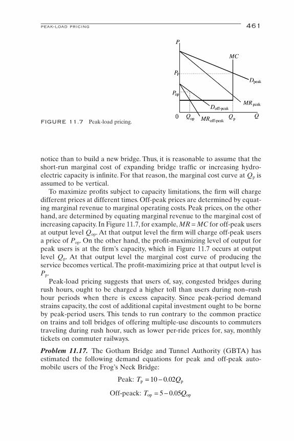
notice than to build a new bridge. Thus, it is reasonable to assume that theshort-run marginal cost of expanding bridge traffic or increasing hydro-electric capacity is infinite. For that reason, the marginal cost curve at Qp isassumed to be vertical.

To maximize profits subject to capacity limitations, the firm will chargedifferent prices at different times. Off-peak prices are determined by equat-ing marginal revenue to marginal operating costs. Peak prices, on the otherhand, are determined by equating marginal revenue to the marginal cost ofincreasing capacity. In Figure 11.7, for example, MR = MC for off-peak usersat output level Qop. At that output level the firm will charge off-peak usersa price of Pop. On the other hand, the profit-maximizing level of output forpeak users is at the firm’s capacity, which in Figure 11.7 occurs at outputlevel Qp. At that output level the marginal cost curve of producing theservice becomes vertical. The profit-maximizing price at that output level isPp.

Peak-load pricing suggests that users of, say, congested bridges duringrush hours, ought to be charged a higher toll than users during non–rushhour periods when there is excess capacity. Since peak-period demandstrains capacity, the cost of additional capital investment ought to be borneby peak-period users. This tends to run contrary to the common practice on trains and toll bridges of offering multiple-use discounts to commuterstraveling during rush hour, such as lower per-ride prices for, say, monthlytickets on commuter railways.

Problem 11.17. The Gotham Bridge and Tunnel Authority (GBTA) hasestimated the following demand equations for peak and off-peak auto-mobile users of the Frog’s Neck Bridge:

Peak:

Off-peack: T Qop op= -5 0 05.

T Qp p= -10 0 02.

peak-load pricing 461

FIGURE 11.7 Peak-load pricing.

where T is the toll charged for a one-minute trip (Q) across the bridge. Themarginal cost of operating the bridge has been estimated at $2 per auto-mobile bridge crossing. The peak capacity of the Frog’s Neck Bridge hasbeen estimated a 50 automobiles per minute. What toll should the GBTAcharge peak and off-peak users of the bridge?

Solution. This is a problem of peak-load pricing. If the GBTA is a profitmaximizer, then off-peak drivers should be charged a price consistent withthe first-order condition for profit maximization, MC = MR. The totalrevenue equation for off-peak users of the bridge is given as

The marginal revenue equation is

Equating marginal revenue to marginal cost yields

Substituting this result into the off-peak demand equation yields the tollcharged to off-peak automobile users of the bridge:

At a bridge capacity of 50 automobiles per minute, the marginal cost curveis vertical. Substituting bridge capacity into the peak demand equationyields the toll that should be charged to peak automobile users of thebridge:

Peak users of the bridge should be charged $9 per crossing.

TRANSFER PRICING

In recent years, the growth of large, conglomerate corporations produc-ing a multitude of products has been accompanied by the parallel devel-opment of semiautonomous profit centers or subsidiaries. The creation ofthese “companies within a company” was an attempt to control rising pro-duction costs that accompanied the burgeoning managerial and adminis-

Tp = - ( ) =10 0 02 50 9. $

T Qop op= - = - ( ) =5 0 05 5 0 05 30 3 50. . $ .

Qop = 30

5 0 1 2- =. Qop

MR MCop op=

MRdTRdQ

Qopop

op= = -5 0 1.

TR T Q Q Q Q Qop op op op op op= = -( ) = -5 0 05 5 0 05 2. .


trative superstructure necessary to coordinate the activities of multiple cor-porate divisions.

Often the output of a division or subsidiary of a parent company is usedas a productive input in the manufacture of the output of another division.A subsidiary of a large, multinational firm, for example, might assembleautomobiles, while another subsidiary manufactures automobile bodies.Still another subsidiary might produce air and oil filters, while yet anotherproduces electronic ignition systems, all of which are used in the produc-tion of automobiles.

Transfer pricing concerns itself with the correct pricing of intermediateproducts that are produced and sold between divisions of a parent company.For example, what price should one division of a company that produces,say, ignition systems, charge another division that assembles automobiles.The optimal pricing of intermediary goods is important because the orga-nizational objective of each division is to maximize profit.What is more, theprice charged for the output of one division that is used as an input in theproduction of another division affects not only each division’s profits butalso profits of the parent company as a whole.

Definition: Transfer pricing involves the optimal pricing of the output ofone subsidiary of a parent company that is sold as an intermediate good toanother subsidiary of the same parent company.

The literature dealing with transfer pricing typically focuses on threepossible scenarios. In the first scenario, there is no external market for theoutput of the division or subsidiary producing the intermediate good. Inother words, the division producing the final product is the sole customerfor the output of the division producing the intermediate good. In thesecond scenario there exists a perfectly competitive external market for theintermediate good. In the third scenario the division or subsidiary operatesin an industry that may be characterized as imperfectly competitive.

TRANSFER PRICING WITH NO EXTERNAL MARKET

Assume that a parent company comprises two subsidiary companies.One subsidiary sells its output, Q1, exclusively to the other subsidiary thatis used in the production of Q2, for final sale in an external market. Assumefurther that there exists no other demand for Q1; that is, there is no exter-nal market for the intermediate good. Finally assume that one unit of Q1 isused to produce one unit of Q2.

Since the parent company comprises only two subsidiaries, the marginalcost of producing Q2 for final sale must include the marginal cost of pro-ducing Q1. The rationale for this is straightforward. Although the companyhas been divided into separate profit centers, in the final analysis thecompany is in the business of producing and selling Q2 for final sale. The

transfer pricing 463

marginal cost of producing Q2 must, of course, include the marginal cost ofproducing Q1. If we assume that the parent company is a profit maximizer,it will produce at the output level where MR2 = MC2. This situation is illus-trated in Figure 11.8.

Since Q1 and Q2 are used on a one-to-one basis, the output level thatmaximizes profit of Q2 will be the same output level as Q1. The selling priceof Q2 is P2. Since the output level of Q1 has been determined by the outputlevel of Q2, the profit-maximizing price for Q1 must be P1 (i.e., where MC1

= MR1). Thus, the correct transfer price for the intermediate good Q1 mustbe P1. It should be noted that any increase in the marginal cost of produc-ing Q1 will result in an increase in the marginal cost of producing Q2, whichwill further result in an increase in the selling price of Q2 and an increasein the transfer price (i.e., the price of the intermediate good that is soldbetween divisions).

On the other hand, suppose that the marginal cost curve of producingQ1 remains unchanged, but the marginal cost curve of producing Q2 shiftsupward, perhaps because of an increase in factor or intermediate goodsprices purchased in the external market. The result will be an increase inP2, a decline in the output of Q2 and Q1, and, assuming an upward slopingmarginal cost curve for Q1, a fall in the transfer price. When the marginalcost of producing Q1 is constant, the transfer price remains unaffected bythe additional increase in the marginal cost of producing Q2.

Problem 11.18. Parallax Corporation produces refractive telescopes foramateur astronomers. The demand equation for Parallax telescopes wasestimated by the operations research department as

Parallax’s total cost equation was estimated as

TC QT T= +100 2 2

Q PT T= -2 000 20,


FIGURE 11.8 Transfer pricing with noexternal market for the intermediate good.

Although the company procures most of its components from outsidevendors, each Parallax telescope requires three highly polished lenses thatare manufactured on site. Because these components are manufactured toexact specifications, there is no outside market for Parallax lenses. The totalcost equation for producing Parallax lenses is

Because of the rapid growth of the company in the 1980s, Parallax man-agement decided to divide the company into two separate profit centers tocontrol costs—the telescope division and the lens division.

a. What is the profit-maximizing price and quantity for Parallax telescopes?b. What is Parallax’s total profit?c. What transfer price should the lens division charge the telescope

division?

Solutiona. Solving the demand equation for PT yields

The corresponding total revenue equation for Parallax telescopes is

The total profit equation for Parallax telescopes is

The first-order condition for profit maximization is dp/dQT = 0. Takingthe first derivative of the profit equation yields

Solving, we have

The second-order condition for profit maximization is dp/dQT < 0. Aftertaking the second derivative of the profit equation, we obtain

which guarantees that this output level represents a local maximum.

ddQ

2

24 1 0

p= - <.

QT * .= 24 39

ddQ

Qp

= - =100 4 1 0. T

pT T T T T T

T T

= - = -( ) - +( )= - + -

TR TC Q Q Q

Q Q

100 0 05 100 2

100 100 2 05

2 2

2

.

.

TR P Q Q Q Q QT T T T T T T= = -( ) = -100 0 05 100 0 05 2. .

P QT T= -100 0 05.

TC QL L= +200 0 025 2.


The profit-maximizing price, therefore, is

b. Parallax’s profit at the profit-maximizing price and quantity is

c. Since there is no external market for Parallax lenses, the transfer priceis equal to the marginal cost of producing the lenses at the profit-maximizing output level. Parallax’s marginal cost equation for pro-ducing lenses is

Since Parallax needs three lenses for every telescope produced, the total number of lenses required by the telescope division is 73.17 lenses(3 ¥ 23.39 telescopes).The marginal cost of producing these lenses, there-fore, is

The transfer price of the lenses, therefore, is $3.51 per lens.

TRANSFER PRICING WITH A PERFECTLYCOMPETITIVE EXTERNAL MARKET

We will now consider the situation in which there exists an externalmarket for the intermediate good. That is, the division or subsidiary pro-ducing the final product has the option of purchasing the intermediate goodeither from a subsidiary of its own parent company or from an outsidevendor. If the intermediate good is purchased from within, what will itstransfer price be? The answer to this question will depend on whether theexternal market for the intermediate good is or is not perfectly competi-tive. We will begin by assuming that there exists a perfectly competitiveexternal market for the intermediate good produced by the subsidiary.

Since both divisions are assumed to be profit maximizers, it stands toreason that the division producing the final good will pay no more for theintermediate good than it would pay in the perfectly competitive externalmarket. Similarly, the division producing the intermediate good will sell itsoutput for nothing less than the perfectly competitive external market price.Thus, the transfer price for the intermediate good is the perfectly competitiveprice in the external market. This situation is depicted in Figure 11.9, wherethe price for the intermediate good is the same price depicted in Figure 11.8.

It should be noted that because the price of the intermediate good inFigure 11.9 is assumed to be the same price depicted in Figure 11.8, the mar-

MC PL L= ( ) = =0 05 70 17 3 51. . $ .

MCdTCdQ

QLL

L= =1 0 05.

p = - + ( ) - ( ) =100 100 24 39 2 05 24 39 1 119 512

. . . $ , .

PT * . . $ .= - ( ) =100 0 05 24 39 98 78


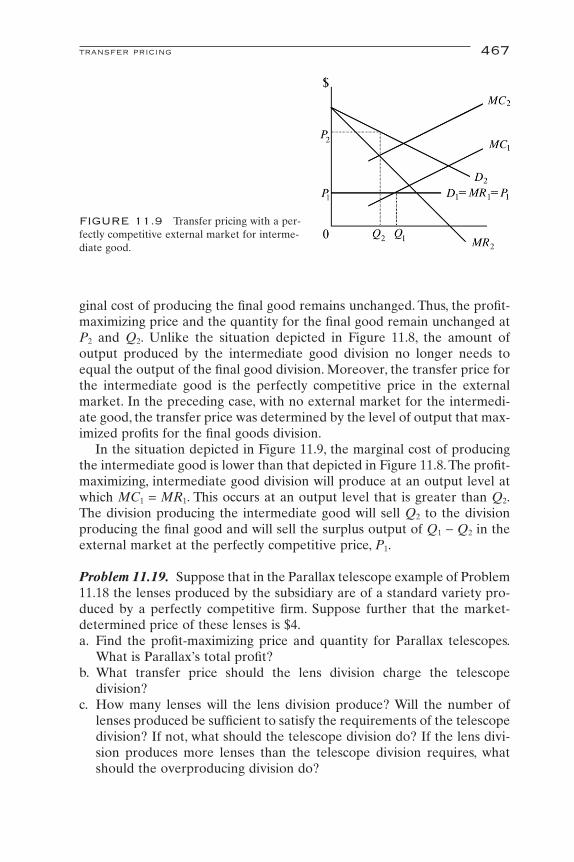
ginal cost of producing the final good remains unchanged. Thus, the profit-maximizing price and the quantity for the final good remain unchanged atP2 and Q2. Unlike the situation depicted in Figure 11.8, the amount ofoutput produced by the intermediate good division no longer needs toequal the output of the final good division. Moreover, the transfer price forthe intermediate good is the perfectly competitive price in the externalmarket. In the preceding case, with no external market for the intermedi-ate good, the transfer price was determined by the level of output that max-imized profits for the final goods division.

In the situation depicted in Figure 11.9, the marginal cost of producingthe intermediate good is lower than that depicted in Figure 11.8. The profit-maximizing, intermediate good division will produce at an output level atwhich MC1 = MR1. This occurs at an output level that is greater than Q2.The division producing the intermediate good will sell Q2 to the divisionproducing the final good and will sell the surplus output of Q1 - Q2 in theexternal market at the perfectly competitive price, P1.

Problem 11.19. Suppose that in the Parallax telescope example of Problem11.18 the lenses produced by the subsidiary are of a standard variety pro-duced by a perfectly competitive firm. Suppose further that the market-determined price of these lenses is $4.a. Find the profit-maximizing price and quantity for Parallax telescopes.

What is Parallax’s total profit?b. What transfer price should the lens division charge the telescope

division?c. How many lenses will the lens division produce? Will the number of

lenses produced be sufficient to satisfy the requirements of the telescopedivision? If not, what should the telescope division do? If the lens divi-sion produces more lenses than the telescope division requires, whatshould the overproducing division do?


FIGURE 11.9 Transfer pricing with a per-fectly competitive external market for interme-diate good.

Solutiona. Since there is no change in the demand for Parallax telescopes, there is

no change in the firm’s total revenue function. However, since lenses arenow $0.49 more expensive than before, Parallax must spend $1.47 moreto produce each telescope. Parallax’s total cost equation for telescopesis now

Parallax’s total profit equation is

The first-order condition for profit maximization is dp/dQT = 0. Takingthe first derivative of the profit equation yields

Solving, we have

The second-order condition for profit maximization is dp/dQT < 0.Takingthe second derivative of the profit equation yields

which guarantees that this output level represents a local maximum. Theprofit-maximizing price, therefore, is

Parallax’s total profit at the profit-maximizing price and quantity is

b. The transfer price for lenses is the price set in the perfectly competitivemarket (i.e., PL = $4).

c. The lens division will maximize profit by setting the marginal cost of pro-ducing lenses equal to the marginal revenue of selling lenses, that is,

Since lens production takes place in a perfectly competitive industry, themarginal revenue from selling lenses is $4 per lens. The marginal costequation of lens production is

MC MRL L=

p = - + ( ) - ( ) =100 98 53 24 03 2 05 24 03 1 083 932

. . . . $ , .

PT * . . $ .= - ( ) =100 0 05 24 03 98 80

ddQ

2

24 1 0

p= - <.

QT * .= 24 03

ddQ

Qp

= - =98 53 4 1 0. . T

p = - = -( ) - + +( )= - + - - = - + -

TR TC Q Q Q Q

Q Q Q Q QT T T T T

T T T T T

100 0 05 100 2 1 47

100 100 2 05 1 47 100 98 53 2 05

2 2

2 2

. .

. . . .

TC Q QTT T= - +100 2 1 472 .


Substitution yields

The lens division should produce 80 lenses. Since the telescope divisionneeds 72.09 lenses (3 ¥ 24.03 telescopes), the lens division should sell theremaining 7.91 lenses in the external market.

TRANSFER PRICING WITH AN IMPERFECTLYCOMPETITIVE EXTERNAL MARKET

Finally, let us consider an imperfectly competitive external market forthe intermediate good. In this case, the price charged by the intermediategood division to the final good division will differ from the price of the inter-mediate good in the imperfectly competitive external market. The pricescharged internally and externally by the intermediate good division becomea matter of third-degree price discrimination. Consider Figure 11.10.

In Figure 11.10, the intermediate good division faces a downward-slopingdemand curve for its output. The total demand for Q1 includes the demandfor the intermediate good by the final-good division and the demand by theexternal market. This demand curve is labeled D1. Once again, the marginalcost of producing the final good Q2 includes the marginal cost of produc-ing Q1.The profit-maximizing level of output for the intermediate good divi-sion is Q1. The corresponding MR1 = MC1 will determine the selling priceof the intermediate good to the final good division. This will be the trans-fer price of the intermediate good.

QL * = 80

4 0 05= . QL

MCdTCdQ

QLL

LL= = 0 05.


FIGURE 11.10 Transfer pricing with an imperfectly competitive external market forthe intermediate good.

The amount of Q1 that will be sold to the final good division will be deter-mined by the profit-maximizing level of output Q2, since Q1 = Q2.This leavesQ1 - Q2 units of Q1 available for sale in the external market. The interme-diate good division will maximize its profits by charging a price in the exter-nal market such that MC1 = MRE. In Figure 11.10, the intermediate gooddivision engages in third-degree price discrimination by charging more inthe external market than it charges the final good division.

OTHER PRICING PRACTICES

This chapter has so far focused on the pricing behavior of profit-maxi-mizing firms operating under somewhat unique circumstances. In each case,the firm’s pricing practices were predicated on subtle economic concepts. Itwas also assumed that management had complete information about therealities of the market in which the firm operated. In practice however, afirm’s pricing practices are much looser in the sense that they are based lesson detailed mathematical analysis than on perception, custom, and intu-ition. The remainder of this chapter is devoted to a review of five of thesealternative pricing practices-price leadership, price skimming, penetrationpricing, prestige pricing, and psychological pricing.

PRICE LEADERSHIP

Price leadership is a phenomenon that is likely to be observed in oli-gopolistic industries. It was noted in Chapter 10 that oligopolistic industriesare characterized by the interdependence of managerial decisions betweenand among the firms in the industry. Firms in oligopolistic industries arekeenly aware that the pricing and output decisions of any individual firmwill provoke a reaction by competing firms. A consequence of this interde-pendence is relatively infrequent price changes.

Definition: Price leadership occurs when a dominant company in anindustry establishes the selling price of a product for the rest of the firmsin the industry. Two forms of price leadership are barometric price leader-ship and dominant price leadership.

Barometric Price Leadership

We saw in our discussion of the kinked demand curve that in oligopo-listic industries, marginal cost may fluctuate within a fairly narrow rangewithout evoking a price change. The reason for this is the discontinuity inthe firm’s marginal revenue curve. As a result, prices are relatively stableat the “kink” in the demand curve. What happens, however, when cost con-ditions for the typical firm in the industry increase significantly because ofsome exogenous shock? How will the increased cost of production mani-


fest itself in the selling price of the product when, for example, the UnitedAuto Workers negotiate higher wages and benefits for union workers in allfirms in the U.S. automobile industry, or OPEC production cutbacks resultin higher energy prices?

Definition: Barometric price leadership occurs when a price change by one firm in an oligopolistic industry, usually in response to perceivedchanges in macroeconomic or market conditions, is quickly followed byprice changes by other firms in the industry.

In an oligopolistic industry characterized by firms of roughly the samesize, price changes may sometimes be explained by barometric price lead-ership. In this case, a typical firm in the industry initiates, say, a price increasebased on management’s belief that changes in macroeconomic or marketconditions will have a uniform impact on all other firms in the industry. Ifother firms believe that the firm’s interpretations of economic events arecorrect, they will quickly follow suit. If they disagree, the firm initiating theprice increase will be forced to reevaluate its decision and may modify orrepeal the price increase. If the price increase is modified, the evaluationprocess begins again. Ultimately, member firms in the industry will form aconsensus and a new, stable, price will be established.

An example of this type of price leadership can be seen in the commer-cial banking industry. Based on its reading of macroeconomic conditions, aleading money-center commercial bank, such as Citibank, may announceits decision to raise or lower the prime rate (the interest rate on loans toits best customers). If the rest of the industry agrees with Citibank’s inter-pretation of macroeconomic conditions, other money-center commercialbanks will quickly follow suit. If not, they will not raise their prime ratesand Citibank will quietly lower its prime rate to a level consistent with thesentiments of the industry.

Dominant Price Leadership

Some industries are characterized by a single, dominant firm and manysmaller competitors. The dominant firm may be the industry leader becauseof its leadership in product innovation, or because of economies of scale. Ifthe firm is large enough or efficient enough, it may be able to force smallercompetitors out of business by undercutting their prices, or it may simplybuy them out. Such behavior, however, often incurs the wrath of the U.S.Department of Justice, which is charged with enforcing federal antitrust legislation.

Definition: Dominant price leadership occurs when one firm in the indus-try is able to establish the industry price as a result of its profit-maximizingbehavior. Once a price has been established by the dominant firm, theremaining firms in the industry become price takers and face a perfectlyelastic demand curve for their output.

other pricing practices 471

Industries dominated by a single large firm are characterized by pricestability. The reason for this is that the dominant firm establishes the sellingprice of the product, and the smaller firms quickly adjust their price andoutput decisions accordingly. This situation is illustrated in Figure 11.11,which indicates that the dominant firm in the industry will behave like amonopolist by producing at output level QD, where its marginal cost is equalto its marginal revenue, MCD = MRD. The profit-maximizing price PI willthen serve as the industry standard. The amount of output provided by therest of the industry will be QI - QD.

What is interesting about this analysis is that once the industry price hasbeen established by the dominant firm, the remaining firms take on theappearance of a perfectly competitive industry in which the demand curvefor their product is perfectly elastic. The other words, other firms in theindustry are price takers. If entry and exit into and from the industry arerelatively easy, the existence of above-normal profits will attract new firmsinto the industry, while below-normal profits will provide an incentive forfirms to leave. It is speculative whether the influx or outflow of firms intothe industry weakens or strengthens the market power of the dominantfirm. In large part, this will depend on the circumstances explaining thefirm’s rise to industry dominance, and whether those factors are sufficientto maintain the firm’s preeminent position.

PRICE SKIMMING

If a firm is first to market with a new product, it may engage in a formof first-degree price discrimination called price skimming. As with first-degree price discrimination, price skimming is an attempt to extract con-sumer surplus. During the interval between the firm’s introduction of a newproduct and the competition’s development of their own versions of thenew product, the innovating firm is a virtual monopoly. If the innovatingfirm wants to extract consumer surplus, however, it must act fast.


FIGURE 11.11 Dominant price leadership.

Definition: Price skimming is an attempt by a firm that introduces a newproduct to extract consumer surplus through differential pricing beforecompetitors develop their own versions of the new product.

The firm begins by initially charging a very high price for its product.Consumers willing and able to pay this price will buy first. Before com-petitors have a chance to sell their versions of the new product, the inno-vating firm will lower its price just a bit to attract the next, lower tier ofconsumers.This process is continued until the price charged equals the mar-ginal cost of production. Pricing in this manner will enable the innovatingfirm to extract consumer surplus to enhance profits. Of course, for thispricing scheme to be successful the firm must have knowledge of thedemand curve of the product. Management is unlikely to have such knowl-edge, however, because of the novel nature of the product. The firm could,of course, conduct consumer surveys, market experiments, and so on, todevelop information regarding the demand for the product, but care wouldhave to be taken not to “tip off” the competition.

PENETRATION PRICING

Penetration pricing occurs when a firm entering a new market charges aprice that is below the prevailing market price to gain a foothold in theindustry. A form of penetration pricing is dumping. Dumping is defined bythe U.S. Department of Commerce as selling a product at less than fairmarket value. The most egregious form of this kind of pricing behavior ispredatory dumping, the attempt by a foreign producer to gain control ofthe market in another country by selling a product there at less than fairmarket value with the goal of driving out domestic producers.

Definition: Penetration pricing is the practice of charging a price that islower than the prevailing market price to gain a foothold in the industry.

PRESTIGE PRICING

Prestige pricing is essentially an attempt by firms to increase sales ofcertain products by capitalizing on snob appeal. Many consumers derive adegree of personal identity from the ostentatious display of certain brand-name items. For them, an enhanced personal image from the conspicuousconsumption of upscale products is as valuable, and sometimes more so,than the usefulness or quality of the product itself. The mere fact that aproduct sells for a higher price often conveys the impression of higherquality, which may or may not be supported by reality. Prestige pricing isan attempt by some firms to exploit this perception by charging higherprices because of the increased prestige that they believe ownership of theirproducts confers. An often cited example is the luxury automobile market,

other pricing practices 473

where higher priced automobiles are perceived to be superior to lowerpriced automobiles of similar quality.

Definition: Prestige pricing is the practice of charging a higher price fora product to exploit the belief by some consumers that a higher price meansbetter quality, which in turn confers on the owner greater prestige.

PSYCHOLOGICAL PRICING

Finally, psychological pricing is a marketing ploy designed to create theillusion in the mind of the consumer that a product is being sold at a sig-nificantly lower price when, in fact, the price differential is inconsequential.Retailer sale of a product for $4.99 instead of $5.00 is psychological pricing.Retailers who engage in psychological pricing are attempting to exploit con-sumers’ initial impressions or their lack of familiarity with the product. Theeffects of psychological pricing tend to be transitory, however, as initialimpressions wear off or the consumer becomes more knowledgeable aboutthe product.

Definition: Psychological pricing is a marketing ploy designed to createthe illusion in the mind of the consumer that a product is being sold at a significantly lower price when, in fact, the price differential is inconsequential.

CHAPTER REVIEW

Earlier chapters discussed output and pricing decisions under some verysimplistic assumptions. We assumed, for example, that profit-maximizingfirms produce a single good or service, that production takes place in asingle location, that these firms sell their products in a well-defined market,that managements have perfect information about production, revenue, andcost functions, and that the firms sell their output at a uniform price to allcustomers. In reality, these assumptions are rarely valid. For that reason, weconsidered alternative pricing practices, which in some cases are derivativesof the more general cases already encountered.

In price discrimination, a firm sells identical products in two or moremarkets at different prices. Economists have identified three degrees ofprice discrimination. First-degree price discrimination occurs when a firmcharges each buyer a different price based on what he or she is willing topay. In practice, first-degree price discrimination is virtually impossible.

In second-degree price discrimination, often referred to as volume dis-counting, different prices are charged for different blocks of units, or dif-ferent products are bundled and sold at a package price. An example ofsecond-degree price discrimination is block pricing, in which there are dif-ferent prices for different blocks of goods and services. Second-degree price


discrimination requires that a firm be able to closely monitor the level ofservices consumed by individual buyers.

In third-degree price discrimination, which is by far the most frequentlypracticed type of price discrimination, firms segment the market for a par-ticular good or service into easily identifiable groups and then charge eachgroup a different price. Such market segregation may be based on suchfactors as geography, age, product use, or income. For third-degree price dis-crimination to be successful, firms must be able to prevent resale of thegood or service across segregated markets.

Cost-plus pricing, also known as markup or full-cost pricing, is anexample of nonmarginal pricing. Firms that engage in nonmarginal pricingare unable or unwilling to devote the resources required to accurately esti-mate the total revenue and total cost equations, or do not know enoughabout demand and cost conditions to determine the profit-maximizing priceand output levels. In cost-plus pricing, a firm sets the selling price of itsproduct as a markup above its fully allocated per-unit cost of production.One criticism of cost-plus pricing is that it is insensitive to demand condi-tions. In practice, however, the size of a firm’s markup tends to be inverselyrelated to the price elasticity of demand for a good or service.

Multi product pricing involves optimal pricing strategies of firms pro-ducing and selling more than one good or service. Firms that independentlyproduce two products with interrelated demands will maximize profits byproducing at a level at which marginal cost is equal to the change in totalrevenue derived from the sale of the product itself, plus the change in totalrevenue derived from the sale of the related product. A profit-maximizingfirm selling two goods with independent demands that are jointly producedin variable proportions will equate the marginal revenue generated fromthe sale of each good to the marginal cost of producing each product.Finally, a profit-maximizing firm that jointly produces two goods in fixedproportions with independent demands will equate the sum of the marginalrevenues of both products expressed in terms of one of the products withthe marginal cost of jointly producing both products expressed in terms ofthe same product.

Peak-load pricing occurs when a profit-maximizing firm charges a oneprice for a service when capacity is fully utilized and a lower price whencapacity is underutilized. Off-peak prices are determined by equating mar-ginal revenue to marginal operating costs. Peak prices, on the other hand,are determined by equating marginal revenue to the marginal cost ofincreasing capacity.

Price leadership appears when an oligopolist establishes a price that isquickly adopted by other firms in the industry. There are two types of priceleadership: barometric price leadership and dominant price leadership.

Barometric price leadership exists when a price change by one firm inan oligopolistic industry, usually in response to perceived changes in macro-

chapter review 475

economic or market conditions, is quickly followed by price changes byother firms in the industry.

Dominant price leadership exists when the largest firm in the industryestablishes the industry price as a result of its profit-maximizing behavior.Once the industry price has been established, the remaining firms becomeprice takers in the sense that they face a perfectly elastic demand curve fortheir output.

Other important pricing practices include transfer pricing, price skim-ming, penetration pricing, prestige pricing, and psychological pricing.

Transfer pricing is a method of correctly pricing a product as it is trans-ferred from one stage of production to another.

Price skimming is the practice of taking advantage of weak or nonexis-tent competition to change a higher price for a new product than is justi-fied by economic analysis.While competitors are trying to catch up, the firmmay have monopoly pricing power.

Penetration pricing is found when a firm entering a new market chargesless than its competitors to gain a foothold in the industry.

Prestige pricing is the setting of a high price for a product in the beliefthat demand will be higher because of the prestige that ownership bestowson the buyer.

Finally, psychological pricing is a marketing ploy designed to create theillusion in the mind of the consumer that a product is being sold at a significantly lower price when, in fact, the price differential is inconse-quential. A retailer that sells a product for $4.99 instead of $5.00 is engag-ing in psychological pricing. The effect of psychological pricing tends to betransitory.

KEY TERMS AND CONCEPTS

Barometric price leadership A price change by one firm in an oligopolis-tic industry, usually in response to perceived changes in macroeconomicor market conditions, quickly followed by price changes by other firmsin the industry.

Block pricing A form of second-degree price discrimination. It involvescharging different prices for different “blocks” of goods and services toenhance profits by extracting at least some consumer surplus.

Commodity bundling Like block pricing, a form or second-degree pricediscrimination. Commodity bundling involves the combining of two ormore different products into a single package, which is sold at a singleprice. Like block pricing, commodity bundling is an attempt to enhanceprofits by extracting at least some consumer surplus.

Consumer surplus The value of benefits received per unit of output con-sumed minus the product’s selling price.


Cost-plus pricing The most popular form of nonmarginal pricing, cost-plus pricing is the practice of adding a predetermined “markup” to afirm’s estimated per-unit cost of production at the time of setting theselling price of its product. Cost-plus pricing is given by the expressionP = ATC(1 + m), where m is the percentage markup and ATC is the fullyallocated per-unit cost of production. The percentage markup may alsobe expressed as m = (P - ATC)/ATC.

Differential pricing Another term for price discrimination. It involvescharging different prices to different groups, for different prices for dif-ferent blocks of goods or services.

Dominant price leadership Establishment of the industry price by thedominant firm in the industry, as a result of its profit-maximizing behav-ior. Once the industry price has been established, the remaining firms inthe industry become price takers and face a perfectly elastic demandcurve for their output.

Dumping Third-degree price discrimination practiced in foreign trade.Anexporting company that sells its product at a different, usually lower,price in the foreign market than it does in the home market is practic-ing dumping.

Dumping margin The difference between the price charged for a productsold by a firm in a foreign market and the price charged in the domes-tic market.

First-degree price discrimination The changing of a different price foreach unit purchased. The price charged for any unit, which is based onthe seller’s knowledge of the individual buyer’s demand curve, reflectsthe consumer’s valuation of each unit purchased. The purpose of first-degree price discrimination is to maximize profits by extracting fromeach consumer the full amount of consumer surplus.

Full-cost pricing Another term for cost-plus pricing.Fully allocated per-unit cost The sum of the estimated average variable

cost of producing a good or service and a per-unit allocation for fixedcost. It is an approximation of average total cost.

Markup pricing Another term for cost-plus pricing.Multiproduct pricing Optimal pricing strategies of a firm producing and

selling more than one good under a number of alternative scenarios,including pricing of two or more goods with interdependent demands,pricing of two or more goods with independent demands produced invariable proportions, pricing of two or more goods with independentdemands jointly produced in fixed proportions, and pricing of two ormore goods given capacity limitations.

Nonmarginal pricing The profit maximizing price and output level aredetermined by equating marginal cost with marginal revenue. Manage-ment will often practice nonmarginal pricing, however, when the firm’stotal cost and total revenue equations are difficult or impossible to esti-

key terms and concepts 477

mate. The most popular form of nonmarginal pricing is cost-plus pricing,also known as markup on full-cost pricing.

Peak-load pricing The practice of charging one price for a service whendemand is high and capacity is fully utilized and a lower price for theservice when demand is low and capacity is underutilized.

Penetration pricing The practice of charging less than the prevailingmarket price to gain a foothold in the industry; a strategy sometimesselected by firms entering a new market.

Prestige pricing The practice of charging a high price for a product toexploit the belief by some consumers that a high price tag means betterquality, which confers upon the owner greater prestige.

Price discrimination The management, by a profit-maximizing firm, tocharge different individuals or groups different prices for the same goodor service.

Price leadership Seen when a dominant company in an industry estab-lishes the selling price of a product for the rest of the firms in the indus-try. Two forms of price leadership are barometric price leadership anddominant price leadership.

Price skimming An attempt by a firm that introduces a new product toextract consumer surplus through differential pricing before the firm’scompetitiors develop their own versions of the new product.

Psychological pricing A marketing ploy designed to create the illusion inthe mind of the consumer that a product is being sold at a significantlylower price when, in fact, the price reduction is inconsequential. Retailersale of a product for $4.99 instead of $5.00 represents psychologicalpricing.

Relationship between the markup and the price elasticity of demand Thesize of a firm’s markup tends to be inversely related to the price elastic-ity of demand for a good or service. When the demand for a product islow, the markup tends to be high, and vice versa. This relationship maybe expressed as m = -1/(ep + 1).

Second-degree price discrimination Similar in principle to first-degreeprice discrimination, it involves products in “blocks” or “bundles” ratherthan one unit at a time.

Third-degree price discrimination Segmenting the market for a particulargood or service into easily identifiable groups, with a different price foreach group.

Transfer pricing The optimal pricing of the output of one subsidiary of aparent company that is sold as an intermediate good to another sub-sidiary of the same parent company.

Two-part pricing A variation of second-degree price discrimination, two-part pricing is an attempt to enhance a firm’s profits by charging a fixedfee for the right to purchase a good or service, plus a per-unit charge.


The per-unit charge is set equal to the marginal cost of providing theproduct, while the fixed fee is used to extract maximum consumersurplus, which is pure profit.

Volume discounting A form of second-degree price discrimination.

CHAPTER QUESTIONS

11.1 Explain each of the following pricing practices.a. First-degree price discriminationb. Second-degree price discriminationc. Third-degree price discrimination11.2 What is consumer surplus?11.3 An important objective of firms engaged that practice price dis-

crimination is the extraction of consumer surplus. Do you agree? Explain.11.4 First-degree price discrimination is a relatively common practice,

especially by firms dealing directly with the public, such as restaurants andretail outlets. Do you agree with this statement? If not, then why not?

11.5 What is the difference between block pricing and commoditybundling?

11.6 Sales of frankfurter rolls in packages of eight or beer in six-packsare examples of what pricing practice? What is the objective of the firm?

11.7 Explain the use of block pricing by amusement parks.Why do someamusement parks engage in block pricing while other, usually older, amuse-ment parks do not?

11.8 The pricing of private goods is fundamentally different from thepricing of public goods because of the properties of excludability anddepletability. Explain.

11.9 Explain how block pricing by amusement parts is similar to blockpricing by cable television companies.

11.10 What is two-part pricing? Provide examples.11.11 Explain how the practice of commodity bundling may give to a

firm an unfair competitive advantage over its rivals.11.12 Explain cost-plus (markup) pricing. Markup pricing suffers from

what theoretical weakness? What are the advantages and disadvantages ofmarkup pricing?

11.13 The more price elastic is the demand for a good or service, thehigher will be the price markup over the marginal cost of production. Doyou agree with this statement? Explain.

11.14 A firm producing two goods with interrelated demands, such aspersonal computers and modems, will maximize profits by equating themarginal revenue generated from the sale of each good separately to the

chapter questions 479

marginal cost of producing each good. Do you agree with this statement?Explain.

11.15 A firm producing in variable proportions two goods with inde-pendent demands, such as automobile taillight and flashlight bulbs, willmaximize profits by equating the marginal cost of producing each good sep-arately to the combined marginal revenue generated from the sale of bothgoods. Do you agree with this statement? Explain.

11.16 A firm producing two goods with independent demands, which areproduced in fixed proportions, will maximize profits by equating the sum ofthe marginal revenues generated from the sale of both goods, expressed interms of one of the goods, to the marginal cost of jointly producing bothgoods. Do you agree? Explain.

11.17 Identify situations in which peak-load pricing may be appropriate.What is the distinguishing characteristic of short-run production functionsin these situations?

11.18 Peak-load pricing suggests that users of commuter railroads becharged higher fares during off-peak hours to compensate the company forlost revenues arising from fewer riders. Do you agree with this statement?Explain.

11.19 Suppose a firm that produces a product for sale in the market alsoproduces a vital component of that good for which there is no outsidemarket. How should the firm “price” this component?

11.20 Explain each of the following pricing practices.a. Barometric price leadershipb. Dominant price leadershipc. Price skimmingd. Penetration pricinge. Prestige pricingf. Psychological pricing

CHAPTER EXERCISES

11.1 Assume that an individual’s demand for a product is

Suppose that the market price of the product $10.a. Approximate the value of this individual’s consumer surplus for

�Q = 1.b. What is value of consumer surplus as �Q Æ 0?11.2 An amusement park has estimated the following demand equation

for the average park guest

Q P= -16 2

Q P= -20 0 5.


where Q represents the number or rides per guest, and P the price per ride.The total cost of providing a ride is characterized by the equation

a. How much should the park charge on a per-ride basis to maximize its profit? What is the amusement park’s total profit per customer?

b. Suppose that the amusement park decides to charge a one-time admission fee. What admission fee will maximize the park’s profit? What is the estimated average profit per park guest?

11.3 A firm sells its product in two separable and identifiable markets.The firm’s total cost of production is

The demand equations for its product in the two markets are

where Q = Q1 + Q2.a. Calculate the firm’s profit-maximizing price and output level in each

market.b. Verify that the demand for the product is less elastic in the market

with the higher price.c. Find the firm’s total profit at the profit-maximizing prices and output

levels.11.4 Ned Bayward practices third-degree price discrimination when

selling barrels of Eastfarthing Leaf in the isolated villages of Toadmortonand Forlorn. The reason for this is that the residents of Toadmorton have aparticular preference for Eastfarthing Leaf, while the people in Forlorn caneither take it or leave it. Ned’s total cost of producing Eastfarthing Leaf isgiven by the equation

The respective demand equations in Forlorn and Toadmorton are

where Q = Q1 + Q2.

QP

2275

7 5= -

.

QP

1150

4 5= -

.

TC Q= +10 0 5 2.

QP

2220

5= -

QP

1110

2= -

TC Q= +5 5

TC Q= +2 0 5.

chapter exercises 481

a. Calculate Ned’s profit-maximizing price and output level in each market.

b. Verify that the demand for Eastfarthing Leaf is less elastic in the Toadmorton than in Forlorn. What does your answer imply about Ned’s pricing policy?

c. Find the firm’s total profit at the profit-maximizing prices and output levels.

11.5 Suppose a company has estimated the average variable cost of pro-ducing its product to be $10. The firms total fixed cost is $100,000.

a. If the company produces 1,000 units and its standard pricing practice is to add a 35% markup, what price should the company charge?

b. Verify that the selling price calculated in part a represents a 35% markup over the estimated average cost of production.

11.6 What is the estimated percentage markup over the fully allocatedper-unit cost of production for the following price elasticities of demand?

a. ep = -10b. ep = -6c. ep = -3d. ep = -2.3e. ep = -1.811.7 A company produces two products, I and F. The demand equation

for F is

The total cost equation is

The company produces product I exclusively as an intermediate good in the production of product F. The total cost equation for producing good Iis

The company is divided into two semiautonomous profit centers: I divisionand the F division.

a. What is the profit-maximizing price and quantity for F division?b. What is F division’s total profit?c. What transfer price should I division charge F division?

SELECTED READINGS

Adams, W. J., and J. I. Yellen. “Commodity Bundling and the Burden of Monopoly.” QuarterlyJournal of Economics, 90 (August 1976), pp. 475–498.

Baye, M. R., and R. O. Beil. Managerial Economics and Business Strategy. Burr Ridge, IL:Richard D. Irwin, 1994.

TC Q1250 0 02= - . I

TC QF F= +100 2 2

Q PF F= -1 500 15,


Benson, B. L., M. L. Greenhut, and G. Norman. “On the Basing Point System.” American Eco-nomic Review, 80 (June 1990), pp. 584–588.

Clemens, E. “Price Discrimination and the Multiple Product Firm.” Review of EconomicStudies, 29 (1950–1951), pp. 1–11.

Darden, B. R. “An Operation Approach to Product Pricing.” Journal of Marketing, April(1968), pp. 29–33.

Hirshleifer, J. “On the Economics of Transfer Pricing.” Journal of Business, July (1956), pp.172–184.

———. “Economics of the Divisional Firm.” Journal of Business, April (1957), pp. 96–108.Keat, P. G., and P. K. Y. Young. Managerial Economics: Economic Tools for Today’s Decision

Makers, 2nd ed. Upper Saddle River, NJ: Prentice Hall, 1996.Lanzillotti, R. F. “Pricing Objectives in Large Companies.” American Economic Review,

December (1958), pp. 921–1040.Littlechild, S. C. “Peak-Load Pricing of Telephone Calls.” The Bell Journal of Economics and

Management Science, Autumn (1970), pp. 191–210.Oi, W. Y. “A Disneyland Dilemma: Two-Part Tariffs for a Mickey Mouse Monopoly.” Quarterly

Journal of Economics, 85 (February 1971), pp. 77–96.Robinson, J. The Economics of Imperfect Competition. London: Macmillan, 1933.Salvatore, D. Managerial Economics. New York: McGraw-Hill, 1989.Schneidau, R. E., and R. D. Knutson.“Price Discrimination in the Food Industry:A Competitive

Stimulant or Tranquilizer?” American Journal of Agricultural Economics,December (1969),pp. 244–246.

Scitovsky, T. “The Benefits of Asymmetric Markets.” Journal of Economic Perspectives, 4(Winter 1990), pp. 135–148.

Silberberg, E. S. The Structure of Economics: A Mathematical Analysis, 3rd ed. New York:McGraw-Hill, 1990.

Steiner, P. O. Peak Loads and Efficient Pricing. Quarterly Journal of Economics, March (1964),pp. 54, 64–76.

Weston, F. J. “Pricing Behavior of Large Firms.” Western Economic Review, December (1958),pp. 1–18.

Williamson, O. E. “Peak-Load Pricing and Optimal Capacity under Indivisibility Constraints.”American Economic Review, September (1966), pp. 56, 810–827.

Wirl, F. “Dynamic Demand and Noncompetitive Pricing Strategies.” Journal of Economics, 54(1991), pp. 105–121.

Yandle, B., Jr. “Monopoly-Induced Third-Degree Price Discrimination.” Quarterly Review ofEconomics and Business, Spring (1971), pp. 71–75.

selected readings 483

This Page Intentionally Left Blank

12

Capital Budgeting

485

Much of the preceding discussion was concerned with the manner inwhich firms organize factors of production during a given period to maxi-mize total economic profits. Clearly this was short-term analysis, with thefocus of managerial decision making primarily on day-to-day, operationalmatters. Whereas short-run profit maximization is certainly important,senior management must also cast an eye to the future well-being of thefirm and its shareholders.As a result, senior management must always ques-tion whether the current product line is adequate to sustain and enhancethe firm’s future profitability, or whether current production capacity is suf-ficient to meet future demand. If production capacity is deemed to be inad-equate to meet future needs, the firm must examine its investment optionsto ascertain its most profitable, risk-adjusted course of action.

This chapter will concentrate on long-term, strategic considerations,focusing primarily on the firm’s investment opportunities. The discussionsin the preceding chapters have dealt almost entirely with per-period profitmaximization. That analysis was fundamentally static. By contrast, invest-ment is fundamentally dynamic, since it involves streams of expendituresand revenues over time. But, $1 received or expended today is worth morethan $1 received or expended tomorrow because the $1 may be investedand earn a rate of return.Thus, an essential element of any investment deci-sion is the proper evaluation of alternative investment opportunities involv-ing alternative initial outlays, expected net returns, and time horizons.

In this chapter we evaluate alternative investment opportunities with different characteristics. Capital budgeting refers to the process of evaluat-ing the comparative net revenues (expenditures on assets less expected

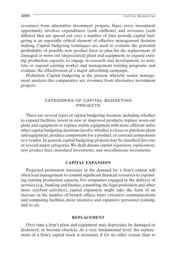
revenues) from alternative investment projects. Since every investmentopportunity involves expenditures (cash outflows) and revenues (cashinflows) that are spread out over a number of time periods, capital bud-geting is an especially critical element of effective management decisionmaking. Capital budgeting techniques are used to evaluate the potentialprofitability of possible new product lines, to plan for the replacement ofdamaged or worn-out (depreciated) plant and equipment, to expand exist-ing production capacity, to engage in research and development, to insti-tute or expand existing worker and management training programs, andevaluate the effectiveness of a major advertising campaign.

Definition: Capital budgeting is the process whereby senior manage-ment analyzes the comparative net revenues from alternative investmentprojects.

CATEGORIES OF CAPITAL BUDGETINGPROJECTS

There are several types of capital budgeting decision, including whetherto expand facilities, invest in new or improved products, replace worn-outplant and equipment or replace usable equipment with more efficient units;other capital budgeting decisions involve whether to lease or purchase plantand equipment, produce components for a product, or contract componentsto a vendor. In general, capital budgeting projects may be classified into oneof several major categories. We shall discuss capital expansion, replacement,new product lines, mandated investments, and miscellaneous investments.

CAPITAL EXPANSION

Projected permanent increases in the demand for a firm’s output willoften lead management to commit significant financial resources to expand-ing existing production capacity. For companies engaged in the delivery ofservices (e.g., banking and finance, consulting, the legal profession and othermore cerebral activities), capital expansion might take the form of anincrease in the number of branch offices, more extensive communicationsand computing facilities, more intensive and expansive personnel training,and so on.

REPLACEMENT

Over time a firm’s plant and equipment may depreciate, be damaged ordestroyed, or become obsolete. At a very fundamental level, the replace-ment of a firm’s capital stock is necessary if for no other reason than to

486 Capital Budgeting

maintain existing output levels to meet existing product demand. Moresubtly, replacement may be necessary to minimize the firm’s cash outflowsarising from, say, maintenance costs, which is a necessary condition for max-imizing the firm’s net revenues and shareholder value.

NEW OR IMPROVED PRODUCT LINES

One of the most important roles of management is to keep abreast ofchanging consumer preferences. Very often, this will require the firm tointroduce new or improved goods and services to satisfy often fickle consumer tastes. Once senior management has decided that a change inconsumer preferences is likely to continue into the foreseeable future,investment in plant and equipment may be necessary to bring new orimproved products to market.

MANDATED INVESTMENTS

The primary obligation of senior management is to satisfy the firm’sinvestors. This obligation often defines the firm’s organizational objective,which is usually the maximization of shareholder returns. This concern forthe return on shareholders’ investment is often tempered, however, by societal or other considerations. These considerations, which often involvequality-of-life issues, such as safety in the workplace or a cleaner environ-ment may entail the construction of access ramps for the disabled or theinstallation of workplace safety equipment and waste disposal facilities,such as “scrubbers” to treat industrial effluents before they are dischargedinto the environment.

Mandated capital expenditures often are not undertaken voluntarilybecause of the obvious negative impact on shareholder returns andcompany’s market share, especially if the firm attempts to pass the increasedcost of production along to the customer. In such cases, municipal, state,and federal regulators often step in to mandate such investment expendi-tures by all firms in an industry, thereby mitigating the competitive disad-vantage to any single firm.

MISCELLANEOUS INVESTMENTS

“Miscellaneous investments” is a catchall for capital budgeting projectsnot easily pigeonholed into any of the foregoing categories. Such capitalbudgeting projects include the construction of employee parking lots, train-ing and personnel development programs, the purchase of executive jets, orany management decision involving an analysis of cash outflows and inflowsthat do not easily fall into traditional capital budgeting classifications.

Categories of Capital Budgeting Projects 487

TIME VALUE OF MONEY

At its core, capital budgeting recognizes that $1 received today does nothave the same value as $1 received tomorrow. Why not? From a psycho-logical perspective it could be argued that, other things being equal, mostpeople prefer the current consumption and enjoyment of a good or aservice to consumption at some future date. There are, however, more prac-tical reasons to conclude that $1 today is worth more than $1 tomorrow. Ifthat $1 were deposited into a savings account paying a certain 5% annualinterest rate, the value of that deposit would be worth $1.05 a year later.Thus, receiving $1 today is worth $1.05 a year from now.

Definition: The time value of money reflects the understanding that adollar received today is worth more than a dollar received tomorrow.

In capital budgeting, future cash inflows and outflows of different capitalinvestment projects are expressed as a single value at a common point intime for purposes of comparison. In most cases, future cash flows areexpressed as a single value at the moment of undertaking the project.

CASH FLOWS

FUTURE VALUE WITH DISCRETE (ANNUAL)COMPOUNDING

The future value of an investment refers to the final accumulated valueof a sum of money at some future time period, usually denoted as t = n. Thefuture value of an investment will depend, of course, not only on the rateof return on that investment, i, but also how often that rate of return is calculated. The frequency of calculation of the rate of return is called compounding.

Definition: Future value is the final accumulated value of a sum of moneyat some future time period.

Definition: Compounding refers to the frequency that the rate of returnon an investment is calculated.

Suppose, for example, that on May 1, 2000 (t = 0) an investor deposits$500 into a certificate of deposit that pays an annually compoundednominal (market) interest rate of 5%. Assume further that the investorplans to make no additional deposits. How much will the certificate ofdeposit be worth on April 30, 2005 (t = 5). It is often useful to visualize suchproblems with a cash flow diagram. Figure 12.1 presents the cash flowdiagram for this problem.

Note that in Figure 12.1 the downward-pointing arrow at t = 0 representsan outflow of $500 as funds are deposited into the certificate of deposit.When the certificate of deposit matures on April 30, 2005, the future value


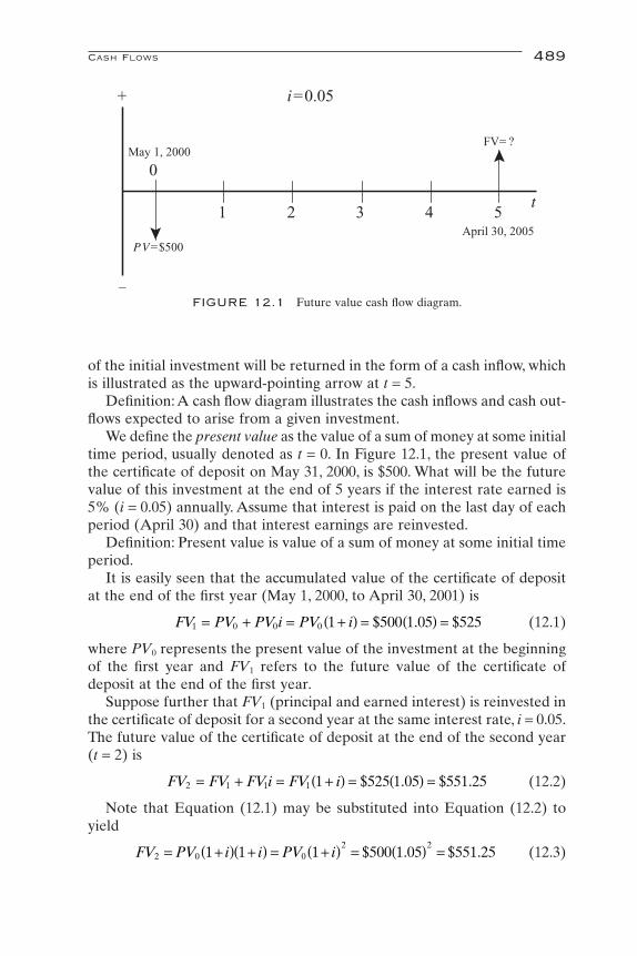
of the initial investment will be returned in the form of a cash inflow, whichis illustrated as the upward-pointing arrow at t = 5.

Definition: A cash flow diagram illustrates the cash inflows and cash out-flows expected to arise from a given investment.

We define the present value as the value of a sum of money at some initialtime period, usually denoted as t = 0. In Figure 12.1, the present value ofthe certificate of deposit on May 31, 2000, is $500. What will be the futurevalue of this investment at the end of 5 years if the interest rate earned is5% (i = 0.05) annually. Assume that interest is paid on the last day of eachperiod (April 30) and that interest earnings are reinvested.

Definition: Present value is value of a sum of money at some initial timeperiod.

It is easily seen that the accumulated value of the certificate of depositat the end of the first year (May 1, 2000, to April 30, 2001) is

(12.1)

where PV0 represents the present value of the investment at the beginningof the first year and FV1 refers to the future value of the certificate ofdeposit at the end of the first year.

Suppose further that FV1 (principal and earned interest) is reinvested inthe certificate of deposit for a second year at the same interest rate, i = 0.05.The future value of the certificate of deposit at the end of the second year(t = 2) is

(12.2)

Note that Equation (12.1) may be substituted into Equation (12.2) toyield

(12.3)FV PV i i PV i2 0 02 2

1 1 1 500 1 05 551 25= +( ) +( ) = +( ) = ( ) =$ . $ .

FV FV FV i FV i2 1 1 1 1 525 1 05 551 25= + = +( ) = ( ) =$ . $ .

FV PV PV i PV i1 0 0 0 1 500 1 05 525= + = +( ) = ( ) =$ . $

Cash Flows 489

+

�

0

1 2 3 4 5t

PV=$500

i=0.05

FV= ?

April 30, 2005

May 1, 2000

FIGURE 12.1 Future value cash flow diagram.

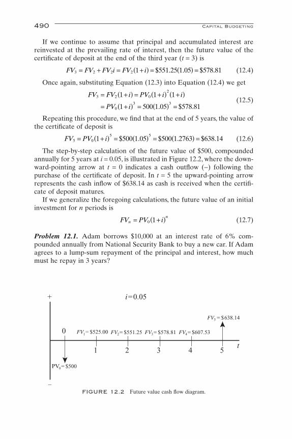
If we continue to assume that principal and accumulated interest arereinvested at the prevailing rate of interest, then the future value of the certificate of deposit at the end of the third year (t = 3) is

(12.4)

Once again, substituting Equation (12.3) into Equation (12.4) we get

(12.5)

Repeating this procedure, we find that at the end of 5 years, the value ofthe certificate of deposit is

(12.6)

The step-by-step calculation of the future value of $500, compoundedannually for 5 years at i = 0.05, is illustrated in Figure 12.2, where the down-ward-pointing arrow at t = 0 indicates a cash outflow (-) following the purchase of the certificate of deposit. In t = 5 the upward-pointing arrowrepresents the cash inflow of $638.14 as cash is received when the certifi-cate of deposit matures.

If we generalize the foregoing calculations, the future value of an initialinvestment for n periods is

(12.7)

Problem 12.1. Adam borrows $10,000 at an interest rate of 6% com-pounded annually from National Security Bank to buy a new car. If Adamagrees to a lump-sum repayment of the principal and interest, how muchmust he repay in 3 years?

FV PV inn= +( )0 1

FV PV i5 05 5

1 500 1 05 500 1 2763 638 14= +( ) = ( ) = ( ) =$ . $ . $ .

FV FV i PV i i

PV i

3 2 02

03 3

1 1 1

1 500 1 05 578 81

= +( ) = +( ) +( )

= +( ) = ( ) =. $ .

FV FV FV i FV i3 2 2 2 1 551 25 1 05 578 81= + = +( ) = ( ) =$ . . $ .


+

�

0

1 2 3 4 5t

PV0= $500

i=0.05

FV1= $525.00 FV2= $551.25 FV3= $578.81 FV4= $607.53

FV5 = $638.14

FIGURE 12.2 Future value cash flow diagram.

Solution. Substituting the information provided into Equation (12.7)yields

This solution is summarized in the cash flow diagram of Figure 12.3.Note, again, that at t = 0 the upward-pointing arrow indicates that

the loan of $10,000 represents a cash inflow (+). At t = 3 the downward-pointing arrow represents the loan repayment and interest payment, whichis a cash outflow (-).

FUTURE VALUE WITH DISCRETE (MOREFREQUENT) COMPOUNDING

The discussion thus far has focused on the future value of a cash amountat some interest rate compounded annually. In most cases, however, inter-est will be compounded more frequently, say semiannually, quarterly, ormonthly. Most bonds, for example, pay interest semiannually; stocks typi-cally pay dividends quarterly, and most mortgages, automobile loans, andstudent loans require monthly payments.

Consider, again, the example illustrated in Figure 12.1. Suppose that thecertificate of deposit pays 5%, which is compounded semiannually.To beginwith, the student should note that the number of compounding periods hasbeen doubled from 5 to 10. Since compounding will occur every 6 monthsinstead of every 12 months, the periodic interest rate is now 2.5% semi-annually instead of 5% per year. With these adjustments, Equation (12.6)may be rewritten as

(12.8)FV PVi

5 0

5 210

12

500 1 025 640 04= +ÊË

ˆ¯ = ( ) =

¥

$ . $ .

FV PV in

3 03

1 10 000 1 06 10 000 1 191 11 910 16= +( ) = ( ) = ( ) =$ , . $ , . $ , .

Cash Flows 491

+

�

0

1 2 3

4 5t

PV0 = $10,000

i = 0.06

FV1= $10,600 FV2 = 11,236

FV3= $11,910.16

FIGURE 12.3 Diagrammatic solution to problem 12.1.

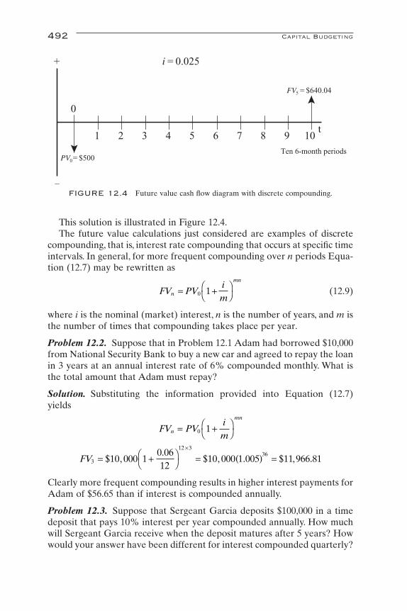
This solution is illustrated in Figure 12.4.The future value calculations just considered are examples of discrete

compounding, that is, interest rate compounding that occurs at specific timeintervals. In general, for more frequent compounding over n periods Equa-tion (12.7) may be rewritten as

(12.9)

where i is the nominal (market) interest, n is the number of years, and m isthe number of times that compounding takes place per year.

Problem 12.2. Suppose that in Problem 12.1 Adam had borrowed $10,000from National Security Bank to buy a new car and agreed to repay the loanin 3 years at an annual interest rate of 6% compounded monthly. What isthe total amount that Adam must repay?


Clearly more frequent compounding results in higher interest payments forAdam of $56.65 than if interest is compounded annually.

Problem 12.3. Suppose that Sergeant Garcia deposits $100,000 in a timedeposit that pays 10% interest per year compounded annually. How muchwill Sergeant Garcia receive when the deposit matures after 5 years? Howwould your answer have been different for interest compounded quarterly?

FV3

12 336

10 000 10 0612

10 000 1 005 11 966 81= +ÊË

ˆ¯ = ( ) =

¥

$ ,.

$ , . $ , .

FV PVimn

mn

= +ÊË

ˆ¯0 1

FV PVimn

mn

= +ÊË

ˆ¯0 1


+

�

0

1 2 3 4 5t

PV0= $500

i = 0.025

FV5 = $640.04

6 7 8 9 10Ten 6-month periods

FIGURE 12.4 Future value cash flow diagram with discrete compounding.

Solution. The future value of Sergeant Garcia’s deposit of $100,000 thatpays an interest rate of 10% compounded annually is

The future value of Sergeant Garcia’s deposit when compounded quarterlyis

FUTURE VALUE WITH CONTINUOUSCOMPOUNDING

Referring to Equation (12.9), what happens as the number of com-pounding periods becomes infinitely large, that is, as m Æ •? This is thecase of continuous compounding. To understand the effect of continuouscompounding on the future value of a particular sum, recall from Chapter2 the definition of the natural logarithm of base e:

(2.50)

Setting 1/h = i/m and substituting into Equation (12.9), we obtain

(12.10)

where i is the interest rate and 1/h is the interest rate per compoundingperiod. Substituting m = hi into Equation (12.10) yields

(12.11)

From Equation (2.50), the limit of Equation (12.11) as h approachesinfinity is

(12.12)

Problem 12.4. Suppose that Adam borrows $10,000 from National Secu-rity Bank and agrees to repay the loan in 3 years at an interest rate of 6%per year, compounded continuously. How much must Adam repay the bankat the end of 3 years?


FV PVh

PVh

PV en h

h i

h

h in

in= +ÊË

ˆ¯

È

ÎÍ

˘

˚˙ = +Ê

Ëˆ¯

È

ÎÍ

˘

˚˙ =Æ• Æ•lim lim0 0 01

11

1

FV PVhn

h in

= +ÊË

ˆ¯

È

ÎÍ

˘

˚˙0 1

1

FV PVim

PVhn

mn mn

= +ÊË

ˆ¯ = +Ê

Ëˆ¯0 01 1

1

ehh

h

= +ÊË

ˆ¯ =Æ•lim . . . .1

12 71829

FV PVimn

mn

= +ÊË

ˆ¯ = +Ê

Ëˆ¯

= ( ) =

¥

0

5 4

20

1 100 000 10 14

100 000 1 025 163 861 64

$ ,.

$ , . $ . .

FV PV inn= +( ) = ( ) = ( ) =0

51 100 000 1 1 100 000 1 61051 161 051$ , . $ , . $ ,

Cash Flows 493

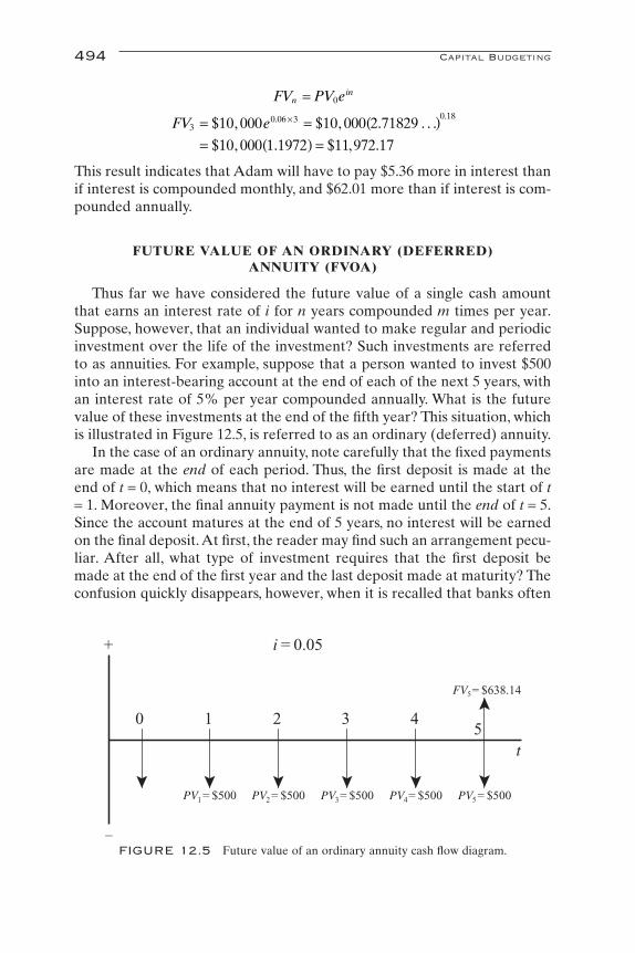
This result indicates that Adam will have to pay $5.36 more in interest thanif interest is compounded monthly, and $62.01 more than if interest is com-pounded annually.

FUTURE VALUE OF AN ORDINARY (DEFERRED)ANNUITY (FVOA)

Thus far we have considered the future value of a single cash amountthat earns an interest rate of i for n years compounded m times per year.Suppose, however, that an individual wanted to make regular and periodicinvestment over the life of the investment? Such investments are referredto as annuities. For example, suppose that a person wanted to invest $500into an interest-bearing account at the end of each of the next 5 years, withan interest rate of 5% per year compounded annually. What is the futurevalue of these investments at the end of the fifth year? This situation, whichis illustrated in Figure 12.5, is referred to as an ordinary (deferred) annuity.

In the case of an ordinary annuity, note carefully that the fixed paymentsare made at the end of each period. Thus, the first deposit is made at theend of t = 0, which means that no interest will be earned until the start of t= 1. Moreover, the final annuity payment is not made until the end of t = 5.Since the account matures at the end of 5 years, no interest will be earnedon the final deposit.At first, the reader may find such an arrangement pecu-liar. After all, what type of investment requires that the first deposit bemade at the end of the first year and the last deposit made at maturity? Theconfusion quickly disappears, however, when it is recalled that banks often

FV e30 06 3 0 18

10 000 10 000 2 71829

10 000 1 1972 11 972 17

= = ( )= ( ) =

¥$ , $ , . . . .

$ , . $ , .

. .

FV PV enin= 0


+

�

0 1 2 3 45

t

i = 0.05

PV1 = $500 PV2 = $500 PV3= $500 PV4= $500

FV5= $638.14

PV5 = $500

FIGURE 12.5 Future value of an ordinary annuity cash flow diagram.

make loans in which the first repayment is not made until the end of thefirst month, with the final payment made at maturity. Such an arrangementis called an amortized loan and represents an investment for the bank.

Definition: An annuity is a series of equal payments, which are made atfixed intervals for a specified number of periods.

Definition: An ordinary (deferred) annuity is an annuity in which thefixed payments are made at the end of each period.

Definition: The future value of an ordinary annuity (FVOA) is the futurevalue of an annuity in which the fixed payments are made at the end ofeach period.

For the situation depicted in Figure 12.5, the future value of the ordinaryannuity may be determined by calculating the sum of the future value ofeach of five separate investments, that is,

Substituting the annuity value and interest rate from Figure 12.5 into theforegoing expression yields

In general, if we denote the constant annuity payment as A, the futurevalue of fixed annuity payments for n periods in which the first payment ismade at the end of t = 0 is

(12.13)

By the algebra of a sum of a geometric progression (see Chapter 2),Equation (12.12) may be rewritten as

(12.14)

Applying Equation (12.14) to the information provided yields the sameoutcome as before:

The value [(1 + i)n -1]/i is referred to as the future value interest factorfor an annuity (FVIFAi,n).

FVOA5

5500 1 05 1

0 05500 0 2763

0 05138 140 05

2 762 82

=( ) -[ ]

=( )

= =

$ .

.$ .

.$ .

.$ , .

FVOAA i

in

n

=+( ) -[ ]1 1

FVOA A i A i A i

A i

nn n

n

t n

= +( ) + +( ) + + +( )

= +( )

- -

-

= ÆÂ1 1 1

1

1 2 0

1

1

. . .

FVOA54 3 2 1

500 1 05 500 1 05 500 1 05 500 1 05 500 1

500 1 21551 500 1 15763 500 1 1025

500 1 05 500 1

607 76 578 81 551 25 525 00 500 2 762 82

= ( ) + ( ) + ( ) + ( ) + ( )= ( ) + ( ) + ( )

+ ( ) + ( )= + + + + =

$ . $ . $ . $ . $

$ . $ . $ .

$ . $

$ . $ . $ . $ . $ $ , .

FVOA PV i PV i PV i PV i PV i5 14

23

32

41

50

1 1 1 1 1= +( ) + +( ) + +( ) + +( ) + +( )

Cash Flows 495

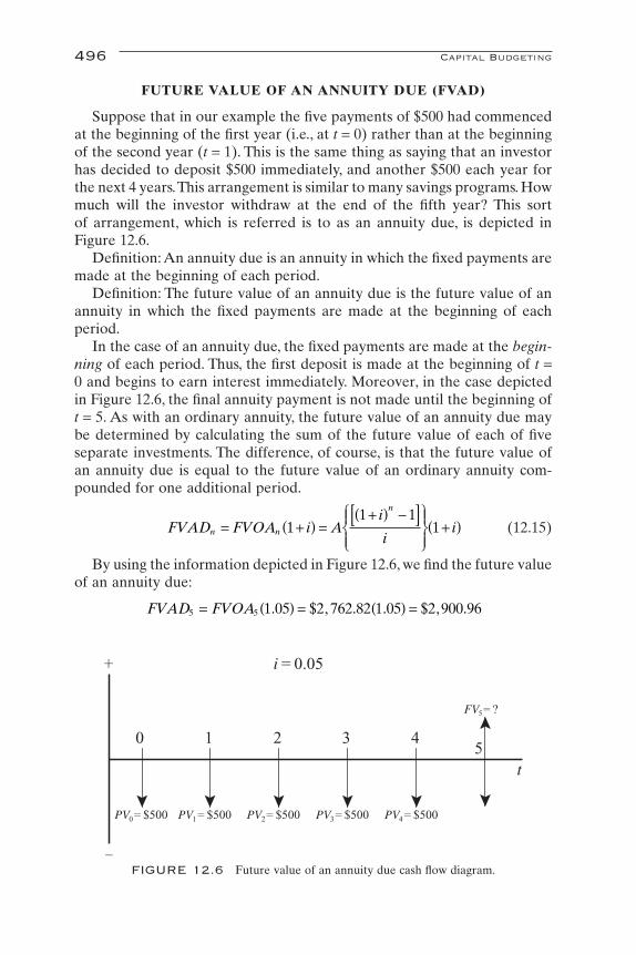
FUTURE VALUE OF AN ANNUITY DUE (FVAD)

Suppose that in our example the five payments of $500 had commencedat the beginning of the first year (i.e., at t = 0) rather than at the beginningof the second year (t = 1). This is the same thing as saying that an investorhas decided to deposit $500 immediately, and another $500 each year forthe next 4 years.This arrangement is similar to many savings programs. Howmuch will the investor withdraw at the end of the fifth year? This sort of arrangement, which is referred is to as an annuity due, is depicted inFigure 12.6.

Definition: An annuity due is an annuity in which the fixed payments aremade at the beginning of each period.

Definition: The future value of an annuity due is the future value of anannuity in which the fixed payments are made at the beginning of eachperiod.

In the case of an annuity due, the fixed payments are made at the begin-ning of each period. Thus, the first deposit is made at the beginning of t =0 and begins to earn interest immediately. Moreover, in the case depictedin Figure 12.6, the final annuity payment is not made until the beginning oft = 5. As with an ordinary annuity, the future value of an annuity due maybe determined by calculating the sum of the future value of each of fiveseparate investments. The difference, of course, is that the future value ofan annuity due is equal to the future value of an ordinary annuity com-pounded for one additional period.

(12.15)

By using the information depicted in Figure 12.6, we find the future valueof an annuity due:

FVAD FVOA5 5 1 05 2 762 82 1 05 2 900 96= ( ) = ( ) =. $ , . . $ , .

FVAD FVOA i Ai

iin n

n

= +( ) =+( ) -[ ]Ï

ÌÔ

ÓÔ

¸˝ÔÔ

+( )11 1

1


+

�

0 1 2 3 45

t

i = 0.05

PV0= $500 PV1 = $500 PV2= $500 PV3= $500

FV5= ?

PV4 = $500

FIGURE 12.6 Future value of an annuity due cash flow diagram.

Compare this amount with the future value of an ordinary annuity of$2,762.82. The difference of $138.14 is attributable to allowing eachpayment of $500 to compound for one additional period.

Problem 12.5. Andrew’s father, Tom, is thinking about putting away a fewdollars away to help pay for his son’s college tuition. Tom would like toinvest $1,000 a year for 10 years into a certificate of deposit. He is reason-ably certain of earning an annual interest rate of 5% per annum over thelife of the investment. Tom is uncertain, however, whether to open the cer-tificate of deposit immediately, or wait until the end of the year to make hisfirst deposit. Tom realizes that by waiting a year before making his depositthat he will lose a full year of interest compounding. On the other hand, hehas the opportunity of earning $100 in interest the first year by lending$1,000 to his Uncle Ned. Assume that Uncle Ned is not a deadbeat and willrepays the loan with interest. Suppose that Tom plans to deposit the $100in interest earned in a regular savings account earning 4% interest annu-ally for 9 years. Should Tom make the loan to Uncle Ned and deposit theinitial $1,000 at the end of the year, or should he open the certificate ofdeposit immediately?

Solution. If Tom decides to deposit $1,000 into a certificate of depositimmediately, the future value of an annuity due is

On the other hand, if Tom decides to wait a year before making the firstdeposit, the future value of an ordinary annuity is

To this amount must be added the future value of $100 received from UncleNed compounded annually for 9 years at an interest rate of 4%. Thisamount is given as

Adding this amount to the future value of an ordinary annuity yields

Since he can make $13,209 by opening the certificate of deposit immedi-ately, Tom will not make the loan to Uncle Ned.

FUTURE VALUE OF AN UNEVEN CASH FLOW

The two preceding sections were devoted to calculating the future valueof an annuity, which is sometimes referred to as an even cash flow. In this

$ , $ . $ , .12 578 143 33 12 721 33+ =

FV PV inn= +( ) = ( ) = ( ) =0

91 100 1 04 100 1 4233 142 33$ . $ . $ .

FVOAA i

in

n

=+( ) -[ ]

=-( )[ ] = ( ) =

1 1 1 000 1 05 10 05

1 000 12 578 12 57810$ , .

.$ , . $ ,

FVAD Ai

iin

n

=+( ) -[ ]Ï

ÌÔ

ÓÔ

¸˝ÔÔ

+( ) =( ) -[ ]Ï

ÌÔ

ÓÔ

¸˝ÔÔ( ) =

1 11 1 000

1 05 1

0 051 05 13 209

10

$ ,.

.. $ ,

Cash Flows 497

section we will discuss the calculation of an uneven cash flow. The futurevalue of an uneven cash flow is determined by compounding each paymentand summing the future values. The future value of an uneven cash flow is sometimes referred to as the terminal value. Figure 12.7 illustrates anuneven cash flow diagram.

The future value of the uneven cash flow may be calculated by repeat-edly applying Equation (12.7). In particular, the present value of an unevencash flow is

(12.16)

The future value of the uneven cash flow depicted in Figure 12.7 at t = 5 is

This solution is illustrated in Figure 12.8.

PRESENT VALUE WITH DISCRETE (ANNUAL)COMPOUNDING

So far we have considered the answer to the question: What will be thevalue of a payment, or series of payments, at the end of a given period oftime? We would now like to turn this around a bit. Suppose that we wereinterested in determining the value an immediate payment, or series of pay-ments, required to grow to a specified value at some time in the future.Suppose, for example, that Adam wanted to know how much he needed toinvest in a certificate of deposit today at 5% interest such that the value of

FV55 4 3 2 1

750 1 042 600 1 042 500 1 042 550 1 042 750 1 042

3752 98

= ( ) + ( ) + ( ) + ( ) + ( )=

. . . . .

$ .

FV PV i PV i PV i

PV i

nn n

tn t

tn t

t n

= +( ) + +( ) + + +( )

= +( )

--

-

-

= ÆÂ

0 11

1

0

1 1 1

1

. . .


+

�

0 1 2 3 4

5t

i = 0 .042

PV0= $750 PV1= $600 PV2= $500 PV3= $550

FV5 = ?

PV4 = $750

FIGURE 12.7 Uneven cash flow.

the investment in 5 years would be $10,000. This amount is referred to asthe present value of the investment. The cash flow diagram for this problemis depicted in Figure 12.9.

Definition: Present value is the value today of an investment, or seriesof investments, that will grow to some future specified amount at a desig-nated rate of interest.

To calculate the present value of a lump-sum investment for n periodsat an interest rate of i, consider again Equation (12.7).

(12.7)

Solving Equation (12.7) for PV0 yields

(12.17)PVFV

i

n

n01

=+( )

FV PV inn= +( )0 1

Cash Flows 499

+

0 1 2 3 4 5t

i = 0.042

�

$921.30

$600 $500 $550 $750$750

707.33565.68597.17781.50

$3,572.98 = FV5

FIGURE 12.8 Future value of an uneven cash flow.

+

�

0

1 2 3 4 5t

PV = ?

i = 0.05

FV = $10,000

FIGURE 12.9 Present value with discrete (annual) compounding.

The present value of an investment, or series of investments, at some des-ignated rate of interest is often referred to as discounted cash flow. The rateof interest that is used to discount a cash flow is called the discount rate.

Definition: A discounted cash flow is the present value of an investmentor series of investments.

Definition: The discount rate is the rate of interest that is used to dis-count a cash flow.

Substituting the foregoing information into Equation (12.17), we findthat the present value of an investment earning 5% interest compoundedannually that will be worth $10,000 in 5 years is

That is, if Adam invests $7,835.26 into a certificate of deposit that earns 5% compounded annually, the value of the investment in 5 years will be$10,000.

Problem 12.6. How much should Turin Turambar invest in a certificate ofdeposit today for that investment to be worth $500 in 7 years if the inter-est rate is 18% per year, compounded annually?

Solution. Substituting this information into Equation (12.17), we find thatthe present value of the investment is

PRESENT VALUE WITH DISCRETE (MOREFREQUENT) AND CONTINUOUS COMPOUNDING

To calculate the present value of a lump-sum investment for n periodsat an interest rate of i compounded m times per period, consider againEquation (12.9).

(12.9)


(12.18)

To calculate the present value of a lump-sum investment for n periodsat an interest rate of i compounded continuously, consider again Equation(12.12).

(12.12)FV PV enin= 0

PVFV

i m

n

mn01

=+( )

FV PVimn

mn

= +ÊË

ˆ¯0 1

PVFV

i

n

n0 71

500

1 18

5003 185

156 96=+( )

=( )

= =$

.

$.

$ .

PV0 5

10 000

1 05

10 0001 276

7 835 26=( )

= =$ ,

.

$ ,.

$ , .



(12.19)

To continue with our example, suppose that Adam wanted to know howmuch he needed to invest in a certificate of deposit today at a 5% interestrate compounded quarterly so that the final value of the investment, 5 yearsfrom now, would be $10,000. Substituting this information into Equation(12.18), we get

How much would the initial investment be if interest were compoundedcontinuously? Substituting this information into Equation (12.19) weobtain

Compare the present value of $10,000 with annual compounding($7,835.26) with the present values where interest is compounded quarterly($7,800.09) and continuously ($7,788.01). Clearly, the more frequent thecompounding, the smaller is the required initial investment.

Problem 12.7. If the prevailing interest rate on a time deposit is 8% peryear, how much would Sergeant Garcia have to deposit today to receive$200,000 at the end of 5 years if the interest rate were compounded quar-terly, monthly, and continuously?

Solution. To receive $200,000 in 5 years on a time deposit that pays 8%compounded quarterly, Sergeant Garcia will have to invest

If interest is compounded monthly, Sergeant Garcia will have to invest

Finally, if interest is compounded continuously Sergeant Garcia will haveto invest

Note, once again, that the more frequent the compounding, the smaller thepresent value, or the amount to be invested at t = 0.

PVFVe e e

n

in0 0 08 5 0 4

200 000 200 000134 064 01= = = =¥

$ , $ ,$ , .

. .

PVFV

i m

n

mn0 12 51

200 000

1 0 08 12134 424 09=

+( )=

+( )=¥

$ ,

.$ , .

PVFV

i m

n

mn0 4 51

200 000

1 0 08 4134 594 27=

+( )=

+( )=¥

$ ,

.$ , .

PVFVe e

n

in0 0 05 5

10 0007 788 01= = =¥

$ ,$ , .

.

PVFV

i m

n

mn0 4 51

10 000

1 0 05 47 800 09=

+( )=

+( )=¥

$ ,

.$ , .

PVFVe

n

in0 =

Cash Flows 501

PRESENT VALUE OF AN ORDINARY ANNUITY (PVOA)

Earlier, we introduced the concept of an annuity as a series of fixed pay-ments made at fixed intervals for a specified period of time. An ordinary(deferred) annuity was defined as a series of payments made at the end ofeach period.Another way to evaluate ordinary annuities is to calculate theirpresent values. In general, the present value of an ordinary annuity may becalculated by using Equation (12.20):

(12.20)

Consider, again, the situation depicted in Figure 12.5, where an investordeposits $500 at the end of each of the next 5 years and earns 5% per yearcompounded annually.What is the present value of these investments at thebeginning of t = 1, which is the same thing as the end of t = 0? Substitutingthe information provided into Equation (12.20), the present value of theannuity due is

The cash flow diagram for this problem is illustrated in Figure 12.10.

Problem 12.8. Suppose that an individual invests $2,500 at the end of eachof the next 6 years and earns an annual interest rate of 8%. Calculate thepresent value of this series of annuity payments.

PVOA5 1 2 3 4 5

500

1 05

500

1 05

500

1 05

500

1 05

500

1 052 164 73=

( )+

( )+

( )+

( )+

( )=

$

.

$

.

$

.

$

.

$

.$ , .

PVOAA

i

A

i

A

i

Ai

n n

t

t n

=+( )

++( )

+ ++( )

=+

ÊË

ˆ¯

= ÆÂ

1 1 1

11

1 2

1

. . .


+

�

0

1 2 3 4 5 t

i = 0.05

$476.19453.51431.92411.35391.76

$2,164.73 = PVOA

$500 $500 $500 $500 $500

FIGURE 12.10 Present value of an ordinary annuity cash flow diagram.


PRESENT VALUE OF AN ANNUITY DUE (PVAD)

As we saw, an annuity due is an annuity in which the fixed payments aremade at the beginning of each period. In general, the present value of anannuity due may be calculated by using Equation (12.21).

(12.21)

By substituting the information provided in Figure 12.7 into Equation(12.21), we find that the present value of an annuity due is

The cash flow diagram for this problem is illustrated in Figure 12.11.

Problem 12.9. Suppose that an individual invests $2,500 at the beginningof each of the next 6 years and earns an annual interest rate of 8%. Calcu-late the value of this series of annuity payments. How does this resultcompare with the solution to Problem 12.8?


PVAD Ain

t n

n t

=+

ÊË

ˆ¯

= Æ

-

Â 110

PVAD5 4 3 2 1 0

500

1 05

500

1 05

500

1 05

500

1 05

500

1 05

411 35 431 92 453 51 476 19 500 2 272 97

=( )

+( )

+( )

+( )

+( )

= + + + + =

$

.

$

.

$

.

$

.

$

.

$ . $ . $ . $ . $ $ , ,

PVADA

n

A

n

A

n

Ai

n n n

n t

t n

=+( )

++( )

+ ++( )

=+

ÊË

ˆ¯

- -

-

= ÆÂ

1 1 1

11

1 2 0

0

. . .

PVOAt

t6

1 6

1 2 3 4 5 6

2 5001

1 0 08

2 500

1 08

2 500

1 08

2 500

1 08

2 500

1 08

2 500

1 02

2 500

1 02

11 557 20

=+

ÊË

ˆ¯

=( )

+( )

+( )

+( )

+( )

+( )

=

= ÆÂ$ ,

.

$ ,

.

$ ,

.

$ ,

.

$ ,

.

$ ,

.

$ ,

.

$ , .

PVOA Ain

t

t n

=+

ÊË

ˆ¯

= ÆÂ 1

11

Cash Flows 503

The present value of an annuity due in this problem is less than thepresent value of an ordinary annuity calculated in Problem 12.8 because

where $2,500/(1.08)6 < $2,500/(1.08)0. In other words, since compoundingtakes place for one less period, PVOA6 > PVAD6.

AMORTIZED LOANS

Amortized loans represent one of the most useful applications of thefuture value of an ordinary annuity. These loans are repaid in equal peri-odic installments. Once again, consider the example in which Adam borrows$10,000 from National Security Bank to buy a new car. Suppose that Adamagrees to repay the loan in 3 years at an interest rate of 6% per year, com-pounded annually. Adam further agrees to repay the loan in equal annualinstallments, with the first installment due at the end of the first year. Howcan he determine the amount of his yearly debt service (principal and inter-est) payments? This problem is depicted in Figure 12.12.

To determine the amount of Adam’s monthly payments, consider againEquation (12.20).

PVOA PVAD6 6 6 0

2 500

1 02

2 500

1 08- =

( )-

( )$ ,

.

$ ,

.

PVADt

n t

61 6

5 4 3 2 1 0

2 5001

1 08

2 500

1 08

2 500

1 08

2 500

1 08

2 500

1 08

2 500

1 08

2 500

1 08

12 481 78

= ÊË

ˆ¯

=( )

+( )

+( )

+( )

+( )

+( )

=

= Æ

-

Â$ ,.

$ ,

.

$ ,

.

$ ,

.

$ ,

.

$ ,

.

$ ,

.

$ , .


+

0 1 2 3 4 5 t

i=0.05

$500.00476.19453.51431.92411.35

$2,272.97 = PVOA

$500 $500 $500 $500$500

–FIGURE 12.11 Present value of an annuity due cash flow diagram.

(12.20)

In this case, we know that PVOA3 = $10,000 and i = 0.06.The task at handis to determine the amount of Adam’s yearly payments, A. Solving Equa-tion (12.20) for A we obtain

(12.22)

Substituting the information provided in the problem into Equation(12.22) and solving yields

Thus, Adam must pay National Security Bank $3,741.11 at the end ofeach of the next three years. Each payment consists of interest due andpartial repayment of principal. This series of repayments is referred to asan amortization schedule. The reader should verify that the largest interestcomponent of the amortization schedule is paid in at the end of the firstyear; thereafter, as the amount of the principal outstanding declines, thepayments are correspondingly less.

Problem 12.10. Suppose that Andrew borrows $250,000 at 3% to purchasea new home. Andrew agrees to repay the loan in 10 equal annual install-ments, with the first payment due at the end of the first year.a. What is the amount of Andrew’s mortgage payments?b. What is the total amount of interest paid?

APVOA

i

n

t nt

=+( )[ ]

=( ) + ( ) + ( )

=

= ÆS 1

2 3

1 1

10 000

1 1 06 1 1 06 1 1 063 741 11

$ ,

. . .$ , .

APVOA

i

n

t nt

=+( )[ ]= ÆS 1 1 1

PVOA Ain

t

t n

=+

ÊË

ˆ¯

= ÆÂ 1

11

Cash Flows 505

+

�

0

1 2 3 4 5

t

i = 0.06

PV0 = $10,000

? ? ?

FIGURE 12.12 Amortized loan cash flow diagram.

Solutiona. Substituting the information provided into Equation (12.22) yields

b. Andrew will make total mortgage payments of 10(29,307.63) =$293,076.27. Thus, the total amount of interest paid will be $293,076.27- $250,000 = $43,076.27.

METHODS FOR EVALUATING CAPITALINVESTMENT PROJECTS

Now that the fundamental techniques for assessing the time value ofmoney have been established, we turn our attention to some of the mostcommonly used methods of assessing the returns on capital investment pro-jects. There are five standard methods for ranking capital investment pro-jects. Each method ranks capital investment projects from the mostpreferred to the least preferred based on the project’s net rate of return(i.e., the rate of return from the investment over and above the total costof financing the project). The cost to the firm of acquiring funds to financea capital investment project is commonly referred to as its cost of capital.

The five most commonly used methods for ranking capital investmentprojects are the payback period, the discounted payback period, the netpresent value (NPV) method, the internal rate of return (IRR), and the mod-ified rate of return (MIRR). We will, illustrate each method by using thehypothetical cash flows (CFt) for projects A and B summarized in Table12.1. To keep the analyses manageable, we will assume that cash flows havebeen adjusted to reflect inflation, taxes, depreciation, and salvage values.

APVOA

i

n

t nt

tt

=+( )[ ]

=+( )[ ]

= =

= Æ

= Æ

S

S

1

1 10

1 1

250 000

1 1 1 03

250 0008 5302

29 307 63$ ,

.

$ ,.

$ , .


TABLE 12.1 Net Cash Flows (CFt) forProjects A and B

Year, t Project A Project B

0 -$25,000 -$25,0001 10,000 3,0002 8,000 5,0003 6,000 7,0004 5,000 9,0005 4,000 11,000

PAYBACK PERIOD METHOD

The payback period of a capital investment project is the number ofperiods required to recover the original investment. In general, the shorterthe payback period, the more preferred the capital investment project.Using the payback period method to evaluate alternative investmentopportunities is perhaps the oldest technique for evaluating capital bud-geting projects.

Definition: The payback period is the number of periods required torecover the original investment.

We can see that for project A by the end of year 3 cumulative cash flowsare $24,000, or 96% of the original investment has been recovered. By theend of year 4 cumulative cash flows are $29,000, or 116% of the originalinvestment has been recovered. Since only an additional $1,000 cash flowwas required in year 4 to fully cover the original $25,000 investment, thenthe total number of years required to recover the original investment (PA)was 3 years plus $1,000/$5,000 years, or 3.2 years. The payback period forProject B (PB) is 4 years plus $1,000/$11,000 years, or 4.09 years In general,the expression for calculating the payback period is

(12.23)

where Pk is the payback period of investment j, (F - 1) is the year beforefull recovery of the original investment, CF0 is the original investment,which is a cash outflow (-), St=1ÆF-1CFt is the sum of all cash flows up to andincluding the year before full recovery of the original investment, and CFF

is the cash flow in the year of full recovery. Substituting the information inTable 12.1 into Equation (12.23) we obtain

Assuming that these projects are mutually exclusive, investment projectA is preferred to project B because project A has a shorter payback period.Projects are said to be mutually exclusive if the acceptance of one projectmeans that all other potential projects are rejected. Projects are said to beindependent if the cash flows from alternative projects are unrelated to eachother.

Definition: Projects are mutually exclusive if acceptance of one projectmeans rejection of all other projects.

Definition: Projects are independent if their cash flows are unrelated.

PB = +- -( ) -

= + =425 000 24 000

11 0004

1 00011 000

4 09$ , $ ,

$ ,$ ,$ ,

. years

PA = +- -( ) -

= + =325 000 24 000

5 0003

1 0005 000

3 20$ , $ ,

$ ,$ ,$ ,

. years

P FCF CF

CFjt F t

F

= -( ) +- -( )= Æ -1 0 1 1S

Methods for Evaluating Capital Investment Projects 507

Problem 12.11. The chief financial analyst of Valaquenta Microprocessors,Inc. has been asked to analyze two proposed capital investment projects,projects A and B. Each project has an initial cost of $10,000. The projectscash flows, which have been adjusted to reflect inflation, taxes, depreciation,and salvage values, are as follows:

Which project should be selected according to the payback periodmethod?

Solution. From the information in Table 12.2, by the end of year 2, the yearbefore full recovery, the cumulative cash flow for project A is $9,500, or95% of the original investment. By the end of year 3, the year of full recov-ery, cumulative cash flows are $11,000, or 110 percent of the original invest-ment. The cumulative cash flow for project B by the end of year 2 is $8,000,or 80% of the original investment. By the end of year 3 the cumulative cashflow for Project B is $12,000, or 120% of the original investment. Substi-tuting the rest of the information in the table into Equation (12.23), we seethat the payback periods for projects A and B are

Thus, project A is preferred to project B because of its shorter paybackperiod.

PCF CF

CFBt t= -( ) +

- -

= +- -( ) - -

= + =

= Æ -3 1

210 000 4 000 4 000

4 0002

2 0004 000

2 50

0 1 3 1

3

S

, , ,,

,,

. years

PCF CF

CFAt t= -( ) +

- -

= +- -( ) - -

= + =

= Æ -3 1

210 000 7 500 2 000

1 5002

5001 500

2 33

0 1 3 1

3

S

, , ,, ,

. years

P FCF CF

CFjt F t

F

= -( ) +- - = Æ -1 0 1 1S




0 -$10,000 -$10,0001 7,500 4,0002 2,000 4,0003 1,500 4,0004 1,000 4,000

DISCOUNTED PAYBACK PERIOD METHOD

A variation on the payback period method is the discounted paybackperiod method. The rationale behind the second method is the same as thatfor the first except that we consider the present value of the projects’ cashflows. The projects are discounted to the present using the investor’s cost ofcapital. The cost of capital is also referred to as the discount rate, therequired rate of return, the hurdle rate, and the cutoff rate. The cost of capital is the opportunity cost of finance capital. It is the minimum rate ofreturn required by an investor to justify the commitment of resources to aproject.

Definition: The cost of acquiring funds to finance a capital investmentproject. It is the minimum rate of return that must be earned to justify acapital investment. The cost of capital is the rate of return that an investormust earn on financial assets committed to a project.

Definition: The discounted payback is the number of periods required to recover the original investment where the projects’ cash flows are discounted using the cost of capital.

Suppose that the initial cost of a project is $25,000 and that cost of capital(k) is 10%.To determine each project’s discounted cash flow (DCFt), simplydivide each period’s cash flow by (1 + k)t. The discounted cash flows for projects A and B are summarized in Table 12.3.

Following the procedure already outlined, we see that for project A bythe end of year 4 cumulative cash flows are $23,625.44, or 94.5% recoveryof the original investment. By the end of year 5 cumulative cash flows are$26, 109.13, or 104.4% recovery of the original investment. Since only anadditional $1,374.56 cash flow was required in year 4 to fully cover the orig-inal $25,000 investment, the total number of years required to recover theoriginal investment (PA) was 4 plus $1,374.56/$2,483.69 years, or 4.55 years.Similarly, the payback period for project B (PB) is 4 plus $6,735.18 years, or4.99 years. As before, project A is preferred to project B. In general, theexpression for calculating the discounted payback period is


TABLE 12.3 Discounted Net CashFlows (DCFt) for Projects A and B


0 -$25,000.00 -$25,000.001 9,090.91 2,727.272 6,611.57 4,132.233 4,507.89 5,259.204 3,415.07 6,146.125 2,483.69 6,830.13

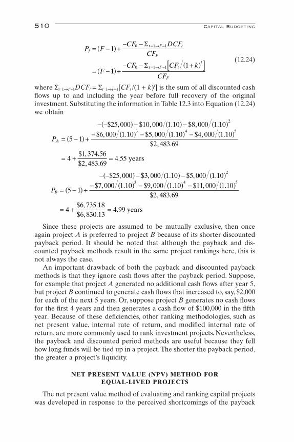
(12.24)

where St=1ÆF-1DCFt = St=1ÆF-1[CFt /(1 + k)t] is the sum of all discounted cashflows up to and including the year before full recovery of the original investment. Substituting the information in Table 12.3 into Equation (12.24)we obtain

Since these projects are assumed to be mutually exclusive, then onceagain project A is preferred to project B because of its shorter discountedpayback period. It should be noted that although the payback and dis-counted payback methods result in the same project rankings here, this isnot always the case.

An important drawback of both the payback and discounted paybackmethods is that they ignore cash flows after the payback period. Suppose,for example that project A generated no additional cash flows after year 5,but project B continued to generate cash flows that increased to, say, $2,000for each of the next 5 years. Or, suppose project B generates no cash flowsfor the first 4 years and then generates a cash flow of $100,000 in the fifthyear. Because of these deficiencies, other ranking methodologies, such asnet present value, internal rate of return, and modified internal rate ofreturn, are more commonly used to rank investment projects. Nevertheless,the payback and discounted period methods are useful because they fellhow long funds will be tied up in a project. The shorter the payback period,the greater a project’s liquidity.

NET PRESENT VALUE (NPV) METHOD FOREQUAL-LIVED PROJECTS

The net present value method of evaluating and ranking capital projectswas developed in response to the perceived shortcomings of the payback

PB = -( ) +

- -( ) - ( ) - ( )- ( ) - ( ) - ( )

= + =

5 1

25 000 3 000 1 10 5 000 1 107 000 1 10 9 000 1 10 11 000 1 10

2 483 69

46 735 186 830 13

4 99

2

3 4 5$ , $ , . $ , .

$ , . $ , . $ , .$ , .

$ , .$ , .

. years

PA = -( ) +

- -( ) - ( ) - ( )- ( ) - ( ) - ( )

= + =

5 1

25 000 10 000 1 10 8 000 1 106 000 1 10 5 000 1 10 4 000 1 10

2 483 69

41 374 562 483 69

4 55

2

3 4 5$ , $ , . $ , .

$ , . $ , . $ , .$ , .

$ , .$ , .

. years

P FCF DCF

CF

FCF CF k

CF

jt F t

F

t F tt

F

= -( ) +- -

= -( ) +- - +( )[ ]

= Æ -

= Æ -

1

11

0 1 1

0 1 1

S

S


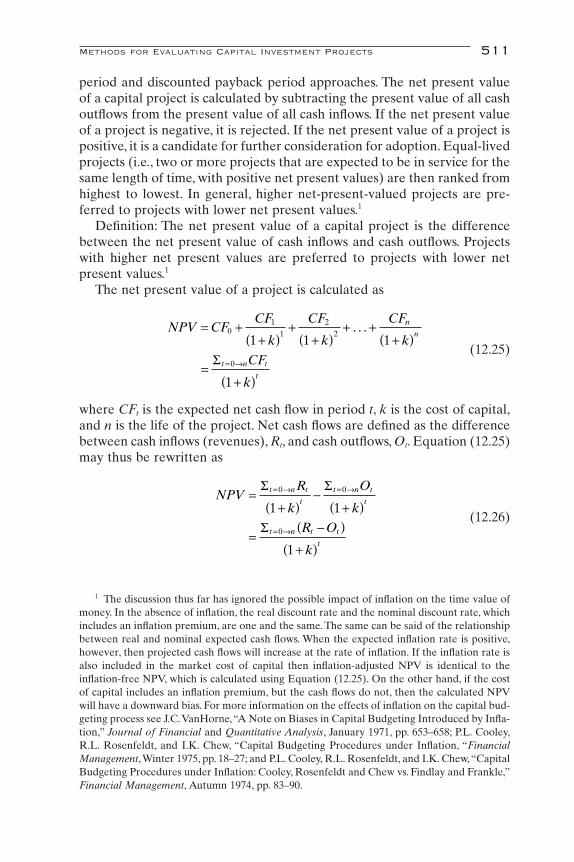
period and discounted payback period approaches. The net present valueof a capital project is calculated by subtracting the present value of all cashoutflows from the present value of all cash inflows. If the net present valueof a project is negative, it is rejected. If the net present value of a project ispositive, it is a candidate for further consideration for adoption. Equal-livedprojects (i.e., two or more projects that are expected to be in service for thesame length of time, with positive net present values) are then ranked fromhighest to lowest. In general, higher net-present-valued projects are pre-ferred to projects with lower net present values.1

Definition: The net present value of a capital project is the differencebetween the net present value of cash inflows and cash outflows. Projectswith higher net present values are preferred to projects with lower netpresent values.1

The net present value of a project is calculated as

(12.25)

where CFt is the expected net cash flow in period t, k is the cost of capital,and n is the life of the project. Net cash flows are defined as the differencebetween cash inflows (revenues), Rt, and cash outflows, Ot. Equation (12.25)may thus be rewritten as

(12.26)

NPVR

k

O

k

R O

k

t n t

t

t n t

t

t n t t

t

=+( )

-+( )

=-( )

+( )

= Æ = Æ

= Æ

S S

S

0 0

0

1 1

1

NPV CFCF

k

CF

k

CF

k

CF

k

n

n

t n t

t

= ++( )

++( )

+ ++( )

=+( )

= Æ

01

1

2

2

0

1 1 1

1

. . .

S


1 The discussion thus far has ignored the possible impact of inflation on the time value ofmoney. In the absence of inflation, the real discount rate and the nominal discount rate, whichincludes an inflation premium, are one and the same. The same can be said of the relationshipbetween real and nominal expected cash flows. When the expected inflation rate is positive,however, then projected cash flows will increase at the rate of inflation. If the inflation rate isalso included in the market cost of capital then inflation-adjusted NPV is identical to the inflation-free NPV, which is calculated using Equation (12.25). On the other hand, if the costof capital includes an inflation premium, but the cash flows do not, then the calculated NPVwill have a downward bias. For more information on the effects of inflation on the capital bud-geting process see J.C.VanHorne,“A Note on Biases in Capital Budgeting Introduced by Infla-tion,” Journal of Financial and Quantitative Analysis, January 1971, pp. 653–658; P.L. Cooley,R.L. Rosenfeldt, and I.K. Chew, “Capital Budgeting Procedures under Inflation, “FinancialManagement,Winter 1975, pp. 18–27; and P.L. Cooley, R.L. Rosenfeldt, and I.K. Chew,“CapitalBudgeting Procedures under Inflation: Cooley, Rosenfeldt and Chew vs. Findlay and Frankle,”Financial Management, Autumn 1974, pp. 83–90.

Consider again the cash flows for projects A and B summarized in Table12.1. Also assume that the cost of capital (k) is 10%. To determine the netpresent value of each project, simply divide the cash flow for each periodby (1 + k)t. The calculation for the net present value of project A (NPVA)is illustrated in Figure 12.13 as $1,109.13. It can just as easily be illustratedthat the net present value of project B is $94.95.

Table 12.4 compares the net present values of projects A and B. If thetwo are independent, then both investments should be undertaken. On theother hand, if projects A and B are mutually exclusive, then project A willbe preferred to project B because its net present value is greater.

A positive net present value indicates that the project is generating cashflows in excess of what is required to cover the cost of capital and to providea positive rate of return to investors. Finally, if the net present value is neg-ative, the present value of cash inflows is not sufficient to cover the presentvalue of cash outflows.A project should not be undertaken if its net presentvalue is negative.


+

0

1 2 3 4 5 t

k = 0.10

�$25,000.009,090.916,611.574,507.89

2,483.69�$1,109.13 = NPVA

$10,000 $8,000 $6,000 $5,000 $4,000

3,415.07

�

FIGURE 12.13 Net present value calculations for project A.

TABLE 12.4 Net Present Value (NPV)for Projects A and B


0 -$25,000.00 -$25,000.001 9,090.91 2,727.272 6,611.57 4,132.233 4,507.89 5,259.204 3,415.07 6,146.125 2,483.69 6,830.13S $1,109.13 $94.95

Problem 12.12. Illuvatar International pays the top corporate income taxrate of 38%. The company is planning to build a new processing plant tomanufacture silmarils on the outskirts of Valmar, the ancient capital ofValinor. The new plant will require an immediate cash outlay of $3 millionbut is expected to generate annual profits of $1 million. According to theValinor Uniform Tax Code, Illuvatar may deduct $500,000 in taxes annu-ally as depreciation. The life of the new plant is 5 years. Assuming that theannual interest rate is 10%, should Illuvatar build the new processing plant?Explain.

Solution. According to the information provided, Illuvatar’s taxable returnis Rt = pt - Dt, where pt represents profits and Dt is the amount of depreci-ation that may be deducted in period t for tax purposes. Illuvatar’s taxablerate of return is

Illuvatar’s annual tax (Tt) is given as Tt = tRt, where t is the tax rate.Illuvatar’s annual tax is, therefore,

Illuvatar’s after tax income flow (pt*) is given as

At an interest rate of 10%, the net present value of the after tax incomeflow is given as

where O0 = $3,000,000, the initial cash outlay. Substituting into this expres-sion, we obtain

Because the net present value is positive, Illuvatar should build the newprocessing plant.

Problem 12.13. Senior management of Bayside Biotechtronics is con-sidering two mutually exclusive investment projects. The projected net cash flows for projects A and B are summarized in Table 12.5. If the dis-count rate (cost of capital) is expected to be 12%, which project should beundertaken?

NPV =( )

+( )

+( )

+( )

+( )

-

=

810 0001 10

810 000

1 10

810 000

1 10

810 000

1 10

810 000

1 103 000 000

70 537 29

2 3 4 5

,.

,

.

,

.

,

.

,

., ,

$ , .

NPVi

O

i

t t t t=+( )

-+( )

= Æ = ÆS S1 5

5

0 0

01 1

p *

p pt t tT* $ , , $ , $ ,= - = - =1 000 000 190 000 810 000

Tt = ( ) =0 38 500 000 190 000. , $ ,

Rt = - =$ , , $ , $ ,1 000 000 500 000 500 000


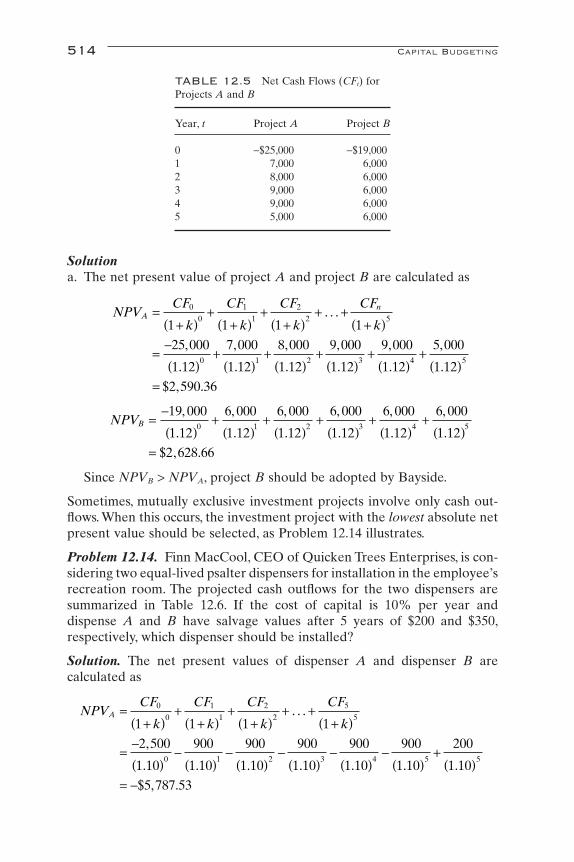
Solutiona. The net present value of project A and project B are calculated as

Since NPVB > NPVA, project B should be adopted by Bayside.

Sometimes, mutually exclusive investment projects involve only cash out-flows. When this occurs, the investment project with the lowest absolute netpresent value should be selected, as Problem 12.14 illustrates.

Problem 12.14. Finn MacCool, CEO of Quicken Trees Enterprises, is con-sidering two equal-lived psalter dispensers for installation in the employee’srecreation room. The projected cash outflows for the two dispensers aresummarized in Table 12.6. If the cost of capital is 10% per year and dispense A and B have salvage values after 5 years of $200 and $350,respectively, which dispenser should be installed?

Solution. The net present values of dispenser A and dispenser B arecalculated as

NPVCF

k

CF

k

CF

k

CF

kA =

+( )+

+( )+

+( )+ +

+( )

=-( )

-( )

-( )

-( )

-( )

-( )

+( )

= -

0

0

1

1

2

2

5

5

0 1 2 3 4 5 5

1 1 1 1

2 500

1 10

900

1 10

900

1 10

900

1 10

900

1 10

900

1 10

200

1 10

5 787 53

. . .

,

. . . . . . .

$ , .

NPVB =-( )

+( )

+( )

+( )

+( )

+( )

=

19 000

1 12

6 000

1 12

6 000

1 12

6 000

1 12

6 000

1 12

6 000

1 12

2 628 66

0 1 2 3 4 5

,

.

,

.

,

.

,

.

,

.

,

.

$ , .

NPVCF

k

CF

k

CF

k

CF

kA

n=+( )

++( )

++( )

+ ++( )

=-( )

+( )

+( )

+( )

+( )

+( )

=

0

0

1

1

2

2 5

0 1 2 3 4 5

1 1 1 1

25 000

1 12

7 000

1 12

8 000

1 12

9 000

1 12

9 000

1 12

5 000

1 12

2 590 36

. . .

,

.

,

.

,

.

,

.

,

.

,

.

$ , .




0 -$25,000 -$19,0001 7,000 6,0002 8,000 6,0003 9,000 6,0004 9,000 6,0005 5,000 6,000

Since |NPVA| < |NPVB|, Finn MacCool will install dispenser A.

Problem 12.15. Suppose that an investment opportunity, which requiresan initial outlay of $50,000, is expected to yield a return of $150,000 after20 years.a. Will the investment be profitable if the cost of capital is 6%?b. Will the investment be profitable if the cost of capital is 5.5%?c. At what cost of capital will the investor be indifferent to the investment?

Solutiona. The net present value of the investment with a cost of capital of 6% is

given as

Since the net present value is negative, we conclude that the investmentopportunity is not profitable.

b. The net present value of the investment with a cost of capital of 5.5% is

Since the net present value is positive, we can conclude that the invest-ment opportunity is profitable.

c. The investor will be indifferent to the investment if the net present valueis zero. Substituting NPV = 0 into the expression and solving for the discount rate yields

NPV =( )

- = - =150 000

1 05550 000

150 0002 92

50 000 1 409 3420

,

.,

,.

, $ , .

NPV =( )

- = - = -150 000

1 0650 000

150 0003 21

50 000 3 229 2920

,

.,

,.

, $ , .

NPVB =-( )

-( )

-( )

-( )

-( )

-( )

+( )

= -

3 500

1 10

700

1 10

700

1 10

700

1 10

700

1 10

700

1 10

350

1 10

5 936 23

0 1 2 3 4 5 5

,

. . . . . . .

$ , .


TABLE 12.6 Net Cash Flows (CFt) forDispensers A and B

Year, t Dispenser A Dispenser B

0 -$2,500 -$3,5001 -900 -7002 -900 -7003 -900 -7004 -900 -7005 -900 -700

That is, the investor will be indifferent to the investment at a cost ofcapital of approximately 5.65%.

NET PRESENT VALUE (NPV) METHOD FORUNEQUAL-LIVED PROJECTS

Whereas comparing alternative investment projects with equal lives is afairly straightforward affair, how do we compare projects that have differ-ent lives? Since net present value comparisons involve future cash flows, anappropriate analysis of alternative capital projects must be compared overthe same number of years. Unless capital projects are compared over anequivalent number of years, there will be a bias against shorter lived capitalprojects involving net cash outflows, and a bias in favor of longer livedcapital projects involving net cash inflows. To avoid this time and cash flowbias when one is evaluating projects with different lives, it is necessary tomodify the net present value calculations to make the projects comparable.

A fair comparison of alternative capital projects requires that net presentvalues be calculated over equivalent time periods. One way to do this is tocompare alternative capital projects over the least common multiple oftheir lives. To accomplish this, the cash flows of each project must be dupli-cated up to the least common multiple of lives for each project. By artifi-cially “stretching out” the lives of some or all of the prospective projectsuntil all projects have the same life span, we can reduce the evaluation ofcapital investment projects with unequal lives to a straightforward applica-tion of the net present value approach to evaluating projects discussed inthe preceding section. In problem 12.16, for example, project A has a lifeexpectancy of 2 years, while project B has a life expectancy of 3 years. Tocompare these two projects by means of the net present value approach,project A will be replicated three times and project B will be replicatedtwice. In this way, both projects will have a 6-year life span.

Problem 12.16. Brian Borumha of Cashel Company, a leading Celtic oilproducer, is considering two mutually exclusive projects, each involvingdrilling operations in the North Sea. The projected net cash flows for eachproject are summarized in Table 12.7. Determine which project should beadopted if the cost of capital is 8%.

0150 000

150 000

50 000 1 150 000

1 3

1 1 05646

0 05647

20

20

20

=+( )

-

+( ) =

+( ) =+ =

=

,,

, ,

.

.

k

k

k

k

k


Solution. Since the projects have different lives, they must be comparedover the least common multiple of years, which in this case is 6 years.

Since NPVB > NPVA, Brian Borumha will select project B over project A.

INTERNAL RATE OF RETURN (IRR) METHODAND THE HURDLE RATE

Yet another method of evaluating a capital investment project is by cal-culating the internal rate of return (IRR). Before discussing the methodol-ogy of calculating a project’s internal rate of return, it is important tounderstand the rationale underlying this approach. Consider, for example,the case of an investor who is considering purchasing a 12-year, 10% annualcoupon, $1,000 par-value corporate bond for $1,150.70. Before decidingwhether the investor should purchase this bond, consider the following definitions.

Coupon bonds are debt obligations of private companies or public agen-cies in which the issuer of the bond promises to pay the bearer of the bonda series of fixed dollar interest payments at regular intervals for a specified

NPVB =-( )

+( )

+( )

+( )

-( )

+( )

+( )

+( )

=

5 000

1 08

1 000

1 08

2 500

1 08

3 000

1 08

5 000

1 08

1 000

1 08

2 500

1 08

3 000

1 08

808 61

0 1 2 3 3

4 5 6

,

.

,

.

,

.

,

.

,

.

,

.

,

.

,

.

$ .

NPVCF

k

CF

k

CF

k

CF

kA =

+( )+

+( )+

+( )+ +

+( )

=-( )

+( )

+( )

-( )

+( )

+( )

-( )

0

0

1

1

2

2

6

6

0 1 2 2 3 4

1 1 1 1

2 000

1 08

1 000

1 08

1 500

1 08

2 000

1 08

1 000

1 08

1 500

1 08

2 000

1 08

. . .

$ ,

.

$ ,

.

$ ,

.

$ ,

.

,

.

,

.

,

.44 5 6

1 000

1 08

1 500

1 08

549 41

+( )

+( )

=

,

.

,

.

$ .


TABLE 12.7 Net Cash Flows (CFt) forProjects A and B ($ millions)


0 -$2,000 -$5,0001 1,000 1,0002 1,500 2,5003 3,000

period of time. Upon maturity, the issuer agrees to repay the bearer the parvalue of the bond. The par value of a bond is the face value of the bond,which is the amount originally borrowed by the issuer. Thus, a corporationthat issues a $1,000 coupon bond is obligated to pay the bearer of the bondfixed dollar payments at regular intervals. In the present example, the issuerof the bond promises to pay the bearer of the bond $100 per year for thenext 12 years plus the face value of the bond at maturity. Parenthetically,the term “coupon bond” comes from the fact that at one time a number ofsmall, dated coupons indicating the amount of interest due to the ownerwere attached to the bonds. A bond owner would literally clip a couponfrom the bond on each payment date and either cash or deposit the couponat a bank or mail it to the corporation’s paying agent, who would then sendthe owner a check in the amount of the interest.

Definition: Coupon bonds are debt obligations in which the issuer of thebond promises to pay the bearer of the bond fixed dollar interest paymentsat regular intervals for a specified period of time, with reimbursement ofthe face value at the end of the period.

Definition: The par value of a bond is the face value of the bond. It isthe amount originally borrowed by the issuer.

Why would an investor consider purchasing a bond for an amount inexcess of its par value? The reason is simple. In the present example, whenthe bond was first issued the prevailing rate of interest paid on bonds withequivalent risk and maturity characteristics was 10%. If the bond holderwanted to sell the bond before maturity, the market price would reflect theprevailing rate of interest.

If current market interest rates are higher than the coupon interest rate,the bearer will have to sell the bond at a discount from par value. Other-wise, no one would be willing to buy such a bond. On the other hand, if pre-vailing interest rates are lower than the coupon interest rate, then the bearerwill be able to sell the bond at a premium. The size of the discount orpremium reflects the term to maturity and the differential between the pre-vailing market interest rate and the coupon rate on bonds with similar riskcharacteristics. Since the market value of the bond in the present exampleis greater than its par value, prevailing market rates must be lower than thecoupon interest rate.

Returning to our example, should the investor purchase this bond? Thedecision to buy or not to buy this bond will be based upon the rate of returnthe investor will earn on the bond if held to maturity. This rate of return iscalled the bond’s yield to maturity (YTM). If the bond’s YTM is greater thanthe prevailing market rate of interest, the investor will purchase the bond.If the YTM is less than the market rate, the investor will not purchase. Ifthe YTM is the same as the market rate, other things being equal, theinvestor will be indifferent between purchasing this bond and a newlyissued bond.


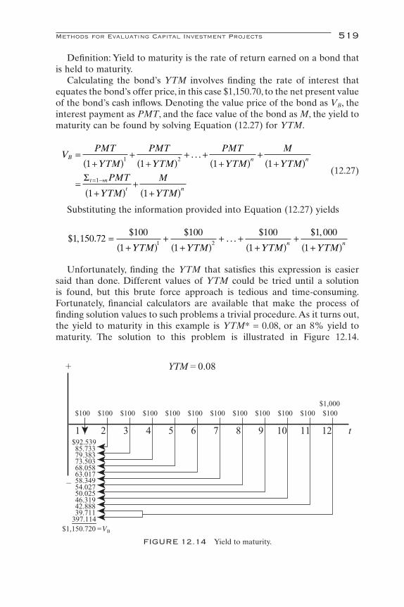
Definition: Yield to maturity is the rate of return earned on a bond thatis held to maturity.

Calculating the bond’s YTM involves finding the rate of interest thatequates the bond’s offer price, in this case $1,150.70, to the net present valueof the bond’s cash inflows. Denoting the value price of the bond as VB, theinterest payment as PMT, and the face value of the bond as M, the yield tomaturity can be found by solving Equation (12.27) for YTM.

(12.27)

Substituting the information provided into Equation (12.27) yields

Unfortunately, finding the YTM that satisfies this expression is easiersaid than done. Different values of YTM could be tried until a solution is found, but this brute force approach is tedious and time-consuming.Fortunately, financial calculators are available that make the process offinding solution values to such problems a trivial procedure. As it turns out,the yield to maturity in this example is YTM* = 0.08, or an 8% yield tomaturity. The solution to this problem is illustrated in Figure 12.14.

$ , .$ $

. . .$ $ ,

1 150 72100

1

100

1

100

1

1 000

11 2

=+( )

++( )

+ ++( )

++( )YTM YTM YTM YTM

n n

VPMT

YTM

PMT

YTM

PMT

YTM

M

YTM

PMT

YTM

M

YTM

B n n

t n

t n

=+( )

++( )

+ ++( )

++( )

=+( )

++( )

= Æ

1 1 1 1

1 1

1 2

1

. . .

S


+

�

1 2 3 4 5 t

YTM = 0.08

6 7 8 9 10 11 12

$100 $100 $100 $100 $100 $100 $100 $100 $100 $100 $100$1,000$100

$92.53985.73379.38373.50368.05863.01758.34954.02750.02546.31942.88839.711

397.114$1,150.720 =VB

FIGURE 12.14 Yield to maturity.

Thus, the investor will compare the YTM to the rate of return on bonds ofequivalent risk characteristics before deciding whether to purchase thebond. Parenthetically, the efficient markets hypothesis suggests that theYTM on this coupon bond will be the same as the prevailing market interest rate.

We now return to the internal rate of return method for evaluatingcapital projects, introduced earlier. As we will see shortly, the methodologyfor determining the yield to maturity on a bond is the same as that used forcalculating the internal rate of return. The internal rate of return is the dis-count rate that equates the present value of a project’s expected cashinflows with the project’s expected cash outflows.The internal rate of returnmay be calculated from Equation (12.28).

(12.28)

Consider, again, the information presented in Table 12.1 for project A.This problem is illustrated in Figure 12.15.

To determine the discount rate for which NPV is zero, substitute theinformation provided for project A in Table 12.1 into Equation (12.27),which yields

NPVIRR IRR IRR

IRR IRR

= - ++( )

++( )

++( )

++( )

++( )

=

$ ,$ , $ , $ ,

$ , $ ,

25 00010 000

1

8 000

1

6 000

1

5 000

1

4 000

10

1 2 3

4 5

NPV CFCF

IRR

CF

IRR

CF

IRR

CF

IRR

n

n

t n t

t

= ++( )

++( )

+ ++( )

=+( )

== Æ

01

1

2

2

1

1 1 1

10

. . .

S


+

0

1 2 3 4 5 t

IRR = ?

�$25,000.00

NPV=0

$10,000 $8,000 $6,000 $5,000 $4,000

t=1 �5PVi =$25,000.00_________

–FIGURE 12.15 Internal rate of return is the discount rate for which the net present valueof a project is equal to zero.

Of course, finding IRR is no easier than solving for YTM, as discussedearlier. Once again, a financial calculator comes to the rescue. The internalrate of return for projects A and B are IRRA = 12.05% and IRRB = 10.12%.Whether these projects are accepted or rejected depends on the cost ofcapital, which is sometimes referred to as the hurdle rate, required rate ofreturn, or cutoff rate. The somewhat colorful expression “hurdle rate” ismeant to express the notion that a company can increase its shareholdervalue by investing in projects that earn a rate of return that exceeds (hurdlesover) the cost of capital used to finance the project.

Definition: The internal rate of return is the discount rate that equatesthe present value of a project’s expected cash inflows with the project’sexpected cash outflows.

Definition: The hurdle rate is the cost of capital of a project that mustbe exceeded by the internal rate of return if the project is to be accepted.Often referred to as the required rate of return or the cutoff rate.

Another way to look at the internal rate of return is that it is themaximum rate of interest that an investor will pay to finance a capitalinvestment project.Alternatively, the internal rate of return is the minimumacceptable rate of return on an investment. Thus, if the internal rate ofreturn is greater than the cost of capital (hurdle rate), a project will beaccepted. If the internal rate of return is less than the hurdle rate, a projectwill be rejected. Finally, if the internal rate of return is equal to the cost ofcapital, the investor will be indifferent to the project. Of course, the investorwould like to earn as much as possible in excess of the internal rate ofreturn.

Suppose that an investor is considering investing in either project A orproject B. If the two projects are independent and the internal rate of returnexceeds the hurdle rate, both projects will be accepted. On the other hand,if the projects are mutually exclusive, project A will be preferred to projectB because of its higher internal rate of return.The NPV and IRR will alwaysresult in the same accept and reject decisions for independent projects. Thisis because, by definition, when NPV is positive, then IRR will exceed thecost of funds to finance the project. On the other hand, the NPV and IRRmethods can result in conflicting accept/reject decisions for mutually exclu-sive projects. A comparison of the NPV and IRR methods of evaluatingcapital investment projects will be the subject of the next section.

Problem 12.17. Consider, again, Bayside Biotechtronics.The projected netcash flows for projects A and B are summarized in Table 12.8.a. Calculate the internal rate of return for both projects.b. If the cost of capital for financing the projects (hurdle rate) is 17%, which

project should be considered?c. Verify that if the hurdle rate is 1% lower, NPVA > 0d. Verify that if the hurdle rate is 1% higher, NPVB < 0.


Solutiona. To determine the internal rate of return for projects A and B, substitute

the information provided in the table into the Equation (12.27) and solvefor IRR.

Since calculating IRRA and IRRB by trial and error is time-consumingand tedious, the solution values were obtained by using a financial cal-culator. The internal rates of return for projects A and B are

b. The internal rate of return is less than the hurdle rate for project A andgreater than the hurdle rate for project B. Thus, project A is rejected andproject B is accepted.

c. Substituting into Equation (12.28), we write

IRR

IRR

A

B

=

=

16 168

17 448

. %

. %

NPVIRR IRR IRR

IRR IRR

B

B B B

B B

= - ++( )

++( )

++( )

++( )

++( )

=

$ ,$ , $ , $ ,

$ , $ ,

19 0006 000

1

6 000

1

6 000

1

6 000

1

6 000

10

1 2 3

4 5

NPV CFCF

IRR

CF

IRR

CF

IRR

IRR IRR IRR

IRR IRR

A

A A A

A A A

A A

= ++( )

++( )

+ ++( )

= - ++( )

++( )

++( )

++( )

++( )

=

01

1

2

2

5

5

1 2 3

4 5

1 1 1

25 0007 000

1

8 000

1

9 000

1

9 000

1

5 000

10

. . .

$ ,$ , $ , $ ,

$ , $ ,


TABLE 12.8 Net Cash Flows CFt forProjects A and B


0 -$25,000 -$19,0001 7,000 6,0002 8,000 6,0003 9,000 6,0004 9,000 6,0005 5,000 6,000

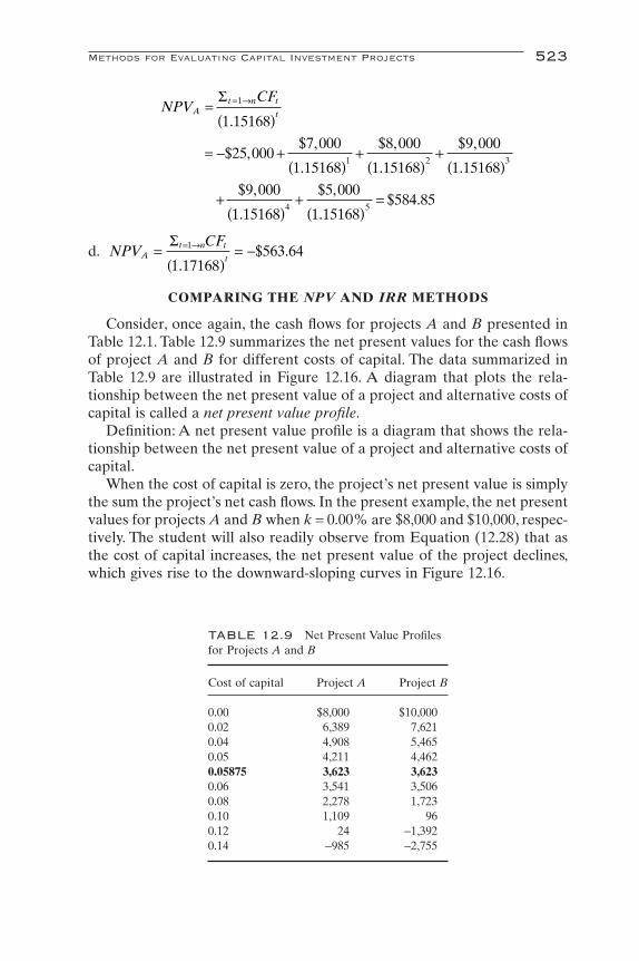
d.

COMPARING THE NPV AND IRR METHODS

Consider, once again, the cash flows for projects A and B presented inTable 12.1. Table 12.9 summarizes the net present values for the cash flowsof project A and B for different costs of capital. The data summarized inTable 12.9 are illustrated in Figure 12.16. A diagram that plots the rela-tionship between the net present value of a project and alternative costs ofcapital is called a net present value profile.

Definition: A net present value profile is a diagram that shows the rela-tionship between the net present value of a project and alternative costs ofcapital.

When the cost of capital is zero, the project’s net present value is simplythe sum the project’s net cash flows. In the present example, the net presentvalues for projects A and B when k = 0.00% are $8,000 and $10,000, respec-tively. The student will also readily observe from Equation (12.28) that asthe cost of capital increases, the net present value of the project declines,which gives rise to the downward-sloping curves in Figure 12.16.

NPVCF

At n t

t=

( )= -= ÆS 1

1 17168563 64

.$ .

NPVCF

At n t

t=

( )

= - +( )

+( )

+( )

+( )

+( )

=

= ÆS 1

1 2 3

4 5

1 15168

25 0007 000

1 15168

8 000

1 15168

9 000

1 15168

9 000

1 15168

5 000

1 15168584 85

.

$ ,$ ,

.

$ ,

.

$ ,

.

$ ,

.

$ ,

.$ .


TABLE 12.9 Net Present Value Profilesfor Projects A and B

Cost of capital Project A Project B

0.00 $8,000 $10,0000.02 6,389 7,6210.04 4,908 5,4650.05 4,211 4,4620.05875 3,623 3,6230.06 3,541 3,5060.08 2,278 1,7230.10 1,109 960.12 24 -1,3920.14 -985 -2,755

In one earlier discussion, the internal rate of return was defined as thediscount rate at which the NPV of a project is zero. For projects A and B,the internal rates of return (not shown in Table 12.9) are 12.05 and 10.12%,respectively. These values are illustrated in Figure 12.16 at the points atwhich the net present value profiles for projects A and B intersect the horizontal axis.

The student will note that when the cost of capital is 5.875%, the netpresent values of projects A and B are the same.Additionally, when the costof capital is less than 5.875% NPVA < NPVB, and when the cost of capitalis greater than 5.875% NPVA > NPVB. This is illustrated in Figure 12.14 atthe point of intersection of the present value profiles of project A and B.For obvious reasons, the cost of capital at which the NPVs of two projectsare equal is called the crossover rate.

Definition: The crossover rate is the cost of capital at which the netpresent values of two projects are equal. Diagrammatically, this is the costof capital at which the net present value profiles of two projects intersect.

An examination of Figure 12.16 also reveals that the marginal change inNPVB given a change in the cost of capital is greater than that for NPVA

(i.e., ∂NPVB/∂k > ∂NPVA/∂k). In other words, the slope of the net presentvalue profile for project B is steeper than the net present value profile forproject A. The reason for this is that project B is more sensitive to changesin the cost of capital than project A.

Given the cost of capital, the sensitivity of NPV to changes in the costof capital will depend on the timing of the project’s cash flows. To see this,consider once again the cash flows summarized in Table 12.1. Note thatthese cash flows are received more quickly in the case of project A than forproject B. Referring to Table 12.9, when the cost of capital is doubled from5.0% to 10.0%, NPVA falls from $4,211 to $1,109, or a decline of 73.7%. Forproject B, NPVB falls from $4,462 to $96, or a drop of 97.8%. The reasonfor the discrepancy is the discounting factor 1/(1 + k)n, which will be greater


NPV

$10,000

$8,000

$3,623

0

NPVB profile

NPVA profile

Crossover

IRRA =12.05%

IRRB =10.12%

4.0 5.5875 8.0 k14.0

FIGURE 12.16 Internal rates of return and crossover rate.

for cash flows received in the distant future than for cash flows received inthe near future. Thus, the net present value of projects that receive greatercash flows in the distant future will decline at a faster rate than for projectsreceiving most of their cash in the early years.

NPV AND IRR METHODS FOR INDEPENDENTPROJECTS

It was noted earlier that when the cost of capital is less than IRR for bothprojects, then the NPV and IRR methods will always result in the sameaccept and reject decisions. This can be seen in Figure 12.16. If the cost ofcapital is less than 10.12%, and projects A and B are independent, both pro-jects will be accepted. If the cost of capital is between 10.12 and 12.05%,project A will be accepted and project B will be rejected. Finally, If the costof capital is greater than 12.05%, then both projects will be rejected.

NPV AND IRR METHODS FOR MUTUALLYEXCLUSIVE PROJECTS

We noted earlier that if the projects are mutually exclusive (the accep-tance of one project means the rejection of the other), the NPV and IRRmethods can result in conflicting accept/reject decisions. To see this, con-sider again Figure 12.16. If the cost of capital is greater than the crossoverrate, but less than IRR for both projects, in this case 10.12%, then NPVA >NPVB and IRRA > IRRB, in which case both the IRR and NPV methodsindicate that project A is preferred to project B.

On the other hand, if the cost of capital is less than the crossover rate,then although IRRA is still less than IRRB, NPVB > NPVA. Thus, the netpresent value method indicates that project B should be preferred toproject A and the internal rate of return method ranks project B higherthan project A. In other words, when the cost of capital is less than thecrossover rate, a conflict arises between the NPV and IRR methods. Twoquestions immediately present themselves:

1. Why do the net present value profiles intersect?2. When an accept/reject conflict exists because the cost of capital is

less than the crossover rate, which method should be used to rankmutually exclusive projects?

The net present value profiles of two projects may intersect for tworeasons: differences in project sizes and cash flow timing differences. Asnoted earlier, the effect of discounting will be greater for cash flowsreceived in the distant future than for cash flows received in the near future.The net present value of projects in which most of the cash flows arereceived in the distant future will decline at a faster rate than the declinein the net present value for projects in which most of the cash flows are


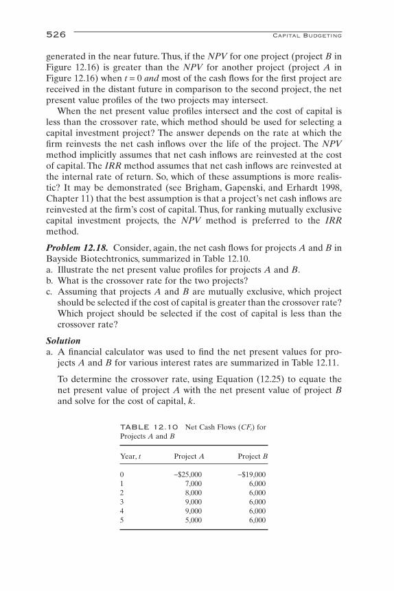
generated in the near future. Thus, if the NPV for one project (project B inFigure 12.16) is greater than the NPV for another project (project A inFigure 12.16) when t = 0 and most of the cash flows for the first project arereceived in the distant future in comparison to the second project, the netpresent value profiles of the two projects may intersect.

When the net present value profiles intersect and the cost of capital isless than the crossover rate, which method should be used for selecting acapital investment project? The answer depends on the rate at which thefirm reinvests the net cash inflows over the life of the project. The NPVmethod implicitly assumes that net cash inflows are reinvested at the costof capital. The IRR method assumes that net cash inflows are reinvested atthe internal rate of return. So, which of these assumptions is more realis-tic? It may be demonstrated (see Brigham, Gapenski, and Erhardt 1998,Chapter 11) that the best assumption is that a project’s net cash inflows arereinvested at the firm’s cost of capital. Thus, for ranking mutually exclusivecapital investment projects, the NPV method is preferred to the IRRmethod.

Problem 12.18. Consider, again, the net cash flows for projects A and B inBayside Biotechtronics, summarized in Table 12.10.a. Illustrate the net present value profiles for projects A and B.b. What is the crossover rate for the two projects?c. Assuming that projects A and B are mutually exclusive, which project

should be selected if the cost of capital is greater than the crossover rate?Which project should be selected if the cost of capital is less than thecrossover rate?

Solutiona. A financial calculator was used to find the net present values for pro-

jects A and B for various interest rates are summarized in Table 12.11.

To determine the crossover rate, using Equation (12.25) to equate thenet present value of project A with the net present value of project Band solve for the cost of capital, k.




0 -$25,000 -$19,0001 7,000 6,0002 8,000 6,0003 9,000 6,0004 9,000 6,0005 5,000 6,000

Bringing all the terms in this expression to the left-hand side of the equation, we get

The value for k in this expression may be found using the IRR functionof a financial calculator. Solving for k yields a crossover rate of 11.72%.

Last, the internal rates of return for projects A and B may be calcu-lated from Equation (12.28).

Solving with a financial calculator yields

IRRA = 16 17. %

NPV CFCF

IRR

CF

IRR

CF

IRR

IRR IRR IRR IRR

IRR IRR

An= +

+( )+

+( )+ +

+( )

=-

+( )+

+( )+

+( )+

+( )

++( )

++( )

=

01

1

2

2 5

0 1 2 3

4 5

1 1 1

25 000

1

7 000

1

8 000

1

9 000

1

9 000

1

9 000

10

. . .

$ , $ , $ , $ ,

$ , $ ,

-

+( )+

+( )+

+( )+

+( )+

+( )-

+( )=

$ , $ , $ , $ , $ , $ ,6 000

1

1 000

1

2 000

1

3 000

1

3 000

1

3 000

10

0 1 2 3 4 5k k k k k k

NPV NPV

k k k k k k

k k k k

A B=

-

+( )+

+( )+

+( )+

+( )+

+( )+

+( )=

-

+( )+

+( )+

+( )+

+( )

$ , $ , $ , $ , $ , $ ,

$ , $ , $ , $ ,

25 000

1

7 000

1

8 000

1

9 000

1

9 000

1

9 000

1

19 000

1

6 000

1

6 000

1

6 000

1

0 1 2 3 4 5

0 1 2 3++

+( )+

+( )$ , $ ,6 000

1

6 000

14 5

k k


TABLE 12.11 Net Present ValueProfiles for Projects A and B

Cost of capital Project A Project B

0.00 $13,000 $11,0000.04 8,931 7,7110.06 7,145 6,2740.08 5,503 4,9560.10 3,989 3,7450.1172 2,780 2,7800.12 2,590 2,6290.14 1,296 1,5980.16 97 6460.18 -1,017 -237

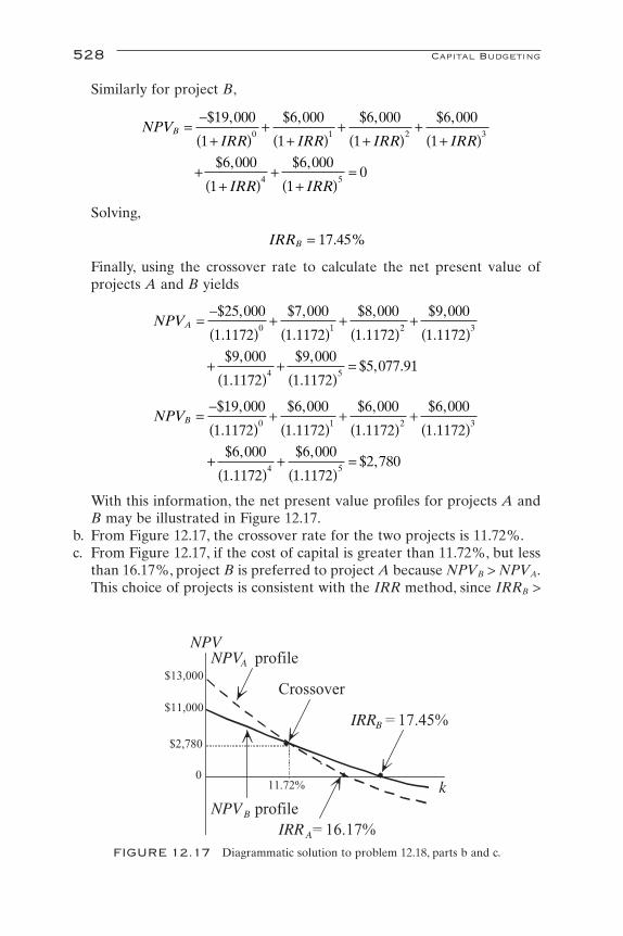
Similarly for project B,

Solving,

Finally, using the crossover rate to calculate the net present value of projects A and B yields

With this information, the net present value profiles for projects A andB may be illustrated in Figure 12.17.

b. From Figure 12.17, the crossover rate for the two projects is 11.72%.c. From Figure 12.17, if the cost of capital is greater than 11.72%, but less

than 16.17%, project B is preferred to project A because NPVB > NPVA.This choice of projects is consistent with the IRR method, since IRRB >

NPVB =-( )

+( )

+( )

+( )

+( )

+( )

=

$ ,

.

$ ,

.

$ ,

.

$ ,

.

$ ,

.

$ ,

.$ ,

19 000

1 1172

6 000

1 1172

6 000

1 1172

6 000

1 1172

6 000

1 1172

6 000

1 11722 780

0 1 2 3

4 5

NPVA =-( )

+( )

+( )

+( )

+( )

+( )

=

$ ,

.

$ ,

.

$ ,

.

$ ,

.

$ ,

.

$ ,

.$ , .

25 000

1 1172

7 000

1 1172

8 000

1 1172

9 000

1 1172

9 000

1 1172

9 000

1 11725 077 91

0 1 2 3

4 5

IRRB = 17 45. %

NPVIRR IRR IRR IRR

IRR IRR

B =-

+( )+

+( )+

+( )+

+( )

++( )

++( )

=

$ , $ , $ , $ ,

$ , $ ,

19 000

1

6 000

1

6 000

1

6 000

1

6 000

1

6 000

10

0 1 2 3

4 5


NPV

$13,000

$11,000

$2,780

0

NPV B profile

NPVA profile

Crossover

IRR A= 16.17%

IRRB = 17.45%

k11.72%

FIGURE 12.17 Diagrammatic solution to problem 12.18, parts b and c.

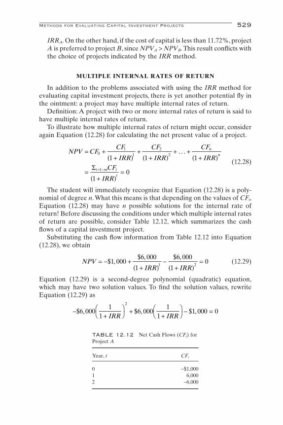
IRRA. On the other hand, if the cost of capital is less than 11.72%, projectA is preferred to project B, since NPVA > NPVB.This result conflicts withthe choice of projects indicated by the IRR method.

MULTIPLE INTERNAL RATES OF RETURN

In addition to the problems associated with using the IRR method forevaluating capital investment projects, there is yet another potential fly inthe ointment: a project may have multiple internal rates of return.

Definition: A project with two or more internal rates of return is said tohave multiple internal rates of return.

To illustrate how multiple internal rates of return might occur, consideragain Equation (12.28) for calculating the net present value of a project.

(12.28)

The student will immediately recognize that Equation (12.28) is a poly-nomial of degree n. What this means is that depending on the values of CFt,Equation (12.28) may have n possible solutions for the internal rate ofreturn! Before discussing the conditions under which multiple internal ratesof return are possible, consider Table 12.12, which summarizes the cashflows of a capital investment project.

Substituting the cash flow information from Table 12.12 into Equation(12.28), we obtain

(12.29)

Equation (12.29) is a second-degree polynomial (quadratic) equation,which may have two solution values. To find the solution values, rewriteEquation (12.29) as

-+

ÊË

ˆ¯ +

+ÊË

ˆ¯ - =$ , $ , $ ,6 000

11

6 0001

11 000 0

2

IRR IRR

NPVIRR IRR

= - ++( )

-+( )

=$ ,$ , $ ,

1 0006 000

1

6 000

10

1 2

NPV CFCF

IRR

CF

IRR

CF

IRR

CF

IRR

n

n

t n t

t

= ++( )

++( )

+ ++( )

=+( )

== Æ

01

1

2

2

1

1 1 1

10

. . .

S


TABLE 12.12 Net Cash Flows (CFt) forProject A

Year, t CFt

0 -$1,0001 6,0002 -6,000

which is of the general form

(2.69)

The solution values may be found by applying the quadratic equation

(2.70)

Substituting the information provided in Equation (12.29) into Equation(2.70) yields

The solution values are

We find that for the cash flows summarized in Table 12.12, this projecthas internal rates of return of both 27 and 476%. The NPV profile for thisproject is summarized in Table 12.13 and Figure 12.18.

Under what circumstances are multiple internal rates of return possible?Thus, far we have dealt only with normal cash flows. A project has normalcash flows when one or more of the cash outflows are followed by a seriesof cash inflows. The cash flow depicted in Table 12.12 is an example of anabnormal cash flow. A large cash outflow during or toward the end of thelife of a project is considered to be abnormal. Projects with abnormal cashflows may exhibit multiple internal rates of return.

Definition: A project has a normal cash flow if one or more cash out-flows are followed by a series of cash inflows.

11

6 000 3 464 1012 000

0 21

1 4 76

3 76

11

6 000 3 464 1012 000

0 79

1 1 27

0 27

1

1

1

2

2

2

+ÊË

ˆ¯ =

- --

=

+( ) ==

+ÊË

ˆ¯ =

- +-

=

+( ) ==

IRR

IRR

IRR

IRR

IRR

IRR

, , .,

.

.

.

, , .,

.

.

.

11

6 000 6 000 4 6 000 1 000

2 6 000

6 000 36 000 000 24 000 00012 000

6 000 12 000 00012 000

6 000 3 464 1012 000

1 2

2 0 5

0 5

0 5

+ÊË

ˆ¯ =

- ± ( ) - -( ) -( )[ ]-( )

=- ± -[ ]

-

=- ± ( )

-

=- ±

-

IRR ,

.

.

.

, , , ,

,

, , , , ,,

, , ,,

, , .,

xb b ac

a1 2

2 0 54

2,

.

=- ± -( )

ax bx c2 0+ + =


Definition: A project has an abnormal cash flow when large cash out-flows occur during or toward the end of the project’s life.

As before, no difficulties arise when the net present value method is usedto evaluate capital investment projects. In our example, if the cost of capitalis between 27 and 376% independent projects should be accepted becausetheir net present value is positive. On the other hand, project selection isproblematic if the internal rate of return method is employed. It may nolonger be automatically presumed that if the internal rate of return isgreater than the cost of capital, the project should be accepted. Suppose,for example, that the cost of capital is 10%, which is less than both internalrates of return. Using the IRR method, which project should be accepted?In general, the approach will be preferred. Using the NPV method,however, the project should be clearly rejected.


TABLE 12.13 Net Present Value Profilefor Project A

k NPV

0.00 -$1,000.000.25 -40.000.27 0.000.50 333.331.00 500.001.50 440.002.00 333.332.50 224.493.00 125.003.50 37.043.76 0.004.00 -40.004.50 -107.44

NPV

0 k

�$1,000

376%

100%

$500

27%

NPV profile

FIGURE 12.18 Multiple internal rates of return.

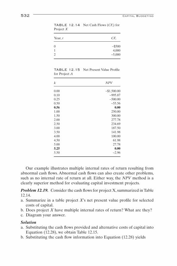
Our example illustrates multiple internal rates of return resulting fromabnormal cash flows. Abnormal cash flows can also create other problems,such as no internal rate of return at all. Either way, the NPV method is aclearly superior method for evaluating capital investment projects.

Problem 12.19. Consider the cash flows for project X, summarized in Table12.14.a. Summarize in a table project X’s net present value profile for selected

costs of capital.b. Does project X have multiple internal rates of return? What are they?c. Diagram your answer.

Solutiona. Substituting the cash flows provided and alternative costs of capital into

Equation (12.28), we obtain Table 12.15.b. Substituting the cash flow information into Equation (12.28) yields


TABLE 12.14 Net Cash Flows (CFt) forProject X

Year, t CFt

0 -$5001 4,0002 -5,000

TABLE 12.15 Net Present Value Profilefor Project A

k NPV

0.00 -$1,500.000.10 -995.870.25 -500.000.50 -55.560.56 0.001.00 250.001.50 300.002.00 277.782.50 234.693.00 187.503.50 141.984.00 100.004.50 61.985.00 27.785.25 0.005.50 -2.96

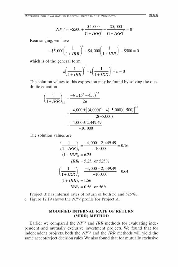
Rearranging, we have

which is of the general form

The solution values to this expression may be found by solving the qua-dratic equation

The solution values are

Project X has internal rates of return of both 56 and 525%.c. Figure 12.19 shows the NPV profile for Project A.

MODIFIED INTERNAL RATE OF RETURN (MIRR) METHOD

Earlier we compared the NPV and IRR methods for evaluating inde-pendent and mutually exclusive investment projects. We found that forindependent projects, both the NPV and the IRR methods will yield thesame accept/reject decision rules. We also found that for mutually exclusive

11

4 000 2 449 4910 000

0 16

1 6 25

5 25 525

11

4 000 2 449 4910 000

0 64

1 1 56

0 56 56

1

1

1

2

2

2

+ÊË

ˆ¯ =

- +-

=

+( ) ==

+ÊË

ˆ¯ =

- --

=

+( ) ==

IRR

IRR

IRR

IRR

IRR

IRR

, , .,

.

.

. , %

, , .,

.

.

. , %

or

or

11

42

4 000 4 000 4 5 000 500

2 5 000

4 000 2 449 4910 000

1 2

2 0 5

2 0 5

+ÊË

ˆ¯ =

- ± -( )

=- ± ( ) - -( ) -( )[ ]

-( )

=- ±

-

IRRb b ac

a,

.

., , ,

,

, , .,

aIRR

bIRR

c1

11

10

2 1

+ÊË

ˆ¯ +

+ÊË

ˆ¯ + =

-+

ÊË

ˆ¯ +

+ÊË

ˆ¯ - =$ , $ , $5 000

11

4 0001

1500 0

2 1

IRR IRR

NPVIRR IRR

= - ++( )

-+( )

=$$ , $ ,

5004 000

1

5 000

10

1 2


capital investment projects the NPV and the IRR methods could result inconflicting accept/reject decision rules.

It was noted that when the net present value profiles of two mutuallyexclusive projects intersect, the choice of projects should be based on theNPV method. This is because the NPV method implicitly assumes that netcash inflows are reinvested at the cost of capital, whereas the IRR methodimplicitly assumes that net cash inflows are reinvested at the internal rateof return. In view of its widespread practical application, is it possible tomodify the IRR method by incorporating into the calculation the assump-tion that net cash flows are reinvested at the cost of capital? Happily, theanswer to this question is yes. What is more, this method also overcomesthe problem of multiple internal rates of return.

The modified internal rate of return (MIRR) method for evaluatingcapital investment projects is similar to the IRR method in that it gener-ates accept/reject decision rules based on interest rate comparisons. Butunlike the IRR method, the MIRR method assumes that cash flows are rein-vested at the cost of capital and avoids some of the problems associatedwith multiple internal rates of return. The modified internal rate of returnfor a capital investment project may be calculated by using Equation (12.30)

(12.30)

where Ot represents cash outflows (costs), Rt represents the project’s cashinflows (revenues), and k is the firm’s cost of capital.

The term on the left hand side of Equation (12.30) is simply the presentvalue of the firm’s investment outlays discounted at the firm’s cost of capital.The numerator on the right side of Equation (12.30) is the future value ofthe project’s cash inflows reinvested at the firm’s cost of capital. The futurevalue of a project’s cash inflows is sometimes referred to as the terminal

S St n t

t

t n tn t

n

O

k

R k

MIRR

= Æ = Æ-

+( )=

+( )+( )

1 1

1

1

1


NPV

0 k

�$1,500

525%

150%

$300

56%

NPV profile

FIGURE 12.19 Diagrammatic solution to problem 12.19.

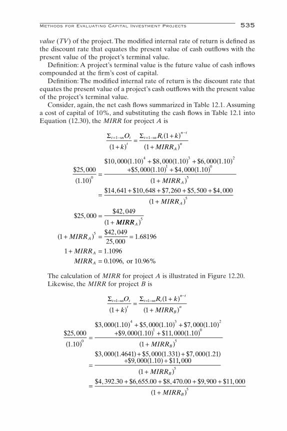
value (TV) of the project. The modified internal rate of return is defined asthe discount rate that equates the present value of cash outflows with thepresent value of the project’s terminal value.

Definition: A project’s terminal value is the future value of cash inflowscompounded at the firm’s cost of capital.

Definition: The modified internal rate of return is the discount rate thatequates the present value of a project’s cash outflows with the present valueof the project’s terminal value.

Consider, again, the net cash flows summarized in Table 12.1. Assuminga cost of capital of 10%, and substituting the cash flows in Table 12.1 intoEquation (12.30), the MIRR for project A is

The calculation of MIRR for project A is illustrated in Figure 12.20.Likewise, the MIRR for project B is

$ ,

.

$ , . $ , . $ , .$ , . $ , .

$ , . $ , . $ , .$ , . $

25 000

1 10

3 000 1 10 5 000 1 10 7 000 1 109 000 1 10 11 000 1 10

1

3 000 1 4641 5 000 1 331 7 000 1 219 000 1 10 11

0

4 3 2

1 0

5( )=

( ) + ( ) + ( )+ ( ) + ( )

+( )

=

( ) + ( ) + ( )+ ( ) +

MIRRB

,,

$ , . $ , . $ , . $ , $ ,

000

1

4 392 30 6 655 00 8 470 00 9 900 11 000

1

5

5

+( )

=+ + + +

+( )

MIRR

MIRR

B

B

S St n t

t

t n tn t

Bn

O

k

R k

MIRR

= Æ = Æ-

+( )=

+( )

+( )1 1

1

1

1

$ ,

.

$ , . $ , . $ , .$ , . $ , .

$ , $ , $ , $ , $ ,

$ ,$ ,

25 000

1 10

10 000 1 10 8 000 1 10 6 000 1 105 000 1 10 4 000 1 10

1

14 641 10 648 7 260 5 500 4 000

1

25 00042 049

1

0

4 3 2

1 0

5

5

( )=

( ) + ( ) + ( )+ ( ) + ( )

+( )

=+ + + +

+( )

=+

MIRR

MIRR

A

A

MIRRMIRR

MIRR

MIRR

MIRR

A

A

A

A

( )

+( ) = =

+ ==

5

51

42 04925 000

1 68196

1 1 1096

0 1096

$ ,,

.

.

. , or 10.96%

S St n t

t

t n tn t

An

O

k

R k

MIRR

= Æ = Æ-

+( )=

+( )+( )

1 1

1

1

1


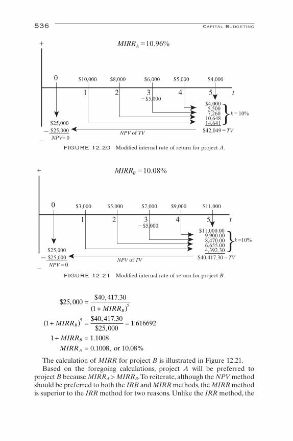
The calculation of MIRR for project B is illustrated in Figure 12.21.Based on the foregoing calculations, project A will be preferred to

project B because MIRRA > MIRRB.To reiterate, although the NPV methodshould be preferred to both the IRR and MIRR methods, the MIRR methodis superior to the IRR method for two reasons. Unlike the IRR method, the

$ ,$ , .

$ , .$ ,

.

.

. ,

25 00040 417 30

1

140 417 30

25 0001 616692

1 1 1008

0 1008

5

5

=+( )

+( ) = =

+ ==

MIRR

MIRR

MIRR

MIRR

B

B

B

A or 10.08%


+

0

1 2 3 4 t

MIRRB =10.08%

$3,000 $5,000 $7,000 $9,000 $11,000

�

5�$5,000

$11,000.009,900.008,470.006,655.004,392.30

$40,417.30 = TV$25,000 $25,000NPV = 0

NPV of TV

�k =10%

–FIGURE 12.21 Modified internal rate of return for project B.

+

0

1 2 3 4 t

MIRRA =10.96%

$10,000 $8,000 $6,000 $5,000 $4,000

�

5�$5,000

$4,0005,5007,260

10,64814,641

$42,049 = TV$25,000 $25,000NPV= 0

NPV of TV

� k = 10%

–FIGURE 12.20 Modified internal rate of return for project A.

MIRR method assumes that cash flows are reinvested at the more defensi-ble cost of capital. Recall that the IRR method assumes that cash flows arereinvested at the firm’s internal rate of return. Moreover, the MIRR methodis not plagued by the problem of multiple internal rates of return.

CAPITAL RATIONING

In each of the methods of evaluating capital investment projects dis-cussed thus far it was implicitly assumed that the firm had unfettered accessto the funds needed to invest in each and every profitable project. If capitalmarkets are efficient, this assumption is approximately true for large, well-established companies with a good record of performance. For smaller, lesswell-established companies, however, easy access to finance capital may belimited. In some cases, finance capital may be relatively easy to obtain, butfor any of a number of reasons senior management may decide to imposea limit on the company’s capital expenditures. Senior management may bereluctant to incur higher levels of debt associated with bank borrowing orwith issuing corporate bonds. Alternatively, senior management may beunwilling to issue equity shares (stock) to raise the requisite financingbecause this will dilute ownership and control. For these and other reasons,senior management may decide to reject potentially profitable projects.

The situation of management-imposed cops on capital expenditures maybe generally described as a problem of capital scarcity.When finance capitalis scarce, the firm’s investment alternatives are said to be constrained, inwhich case whatever finance capital is available should be used as efficientlyas possible. The process of allocating scarce finance capital as efficiently aspossible is called capital rationing.

Definition: Capital rationing refers to the efficient allocation of scarcefinance capital.

Although details of the procedures involved in efficiently allocatingscarce capital are beyond the scope of the present discussion, a simpleexample will convey the spirit of the capital rationing process. Assume thatsenior management has $1,000 to invest in six independent projects, eachwith a life expectancy of 5 years. Assume also that the firm’s cost of capitalis 5% per year. Table 12.16 summarizes the net present values of six feasi-ble capital investment projects.

It is readily apparent from Table 12.16 that $1,250 in finance capital willbe required for the firm to undertake all six projects for a maximum netpresent value of $945. The problem, of course, is that the firm only has$1,000 to invest. Given this constraint, which projects should the firm under-take to maximize the net present value of $1,000?

The question confronting senior management is this: Which projectsshould be selected? Table 12.17 ranks from highest to lowest the alterna-

Capital Rationing 537

tives available to the firm based on total net present value. Table 12.17assumes that any residual funds not allocated to a project are invested for5 years at the firm’s cost of capital.

For senior management to generate the highest total net present value,the information presented in Table 12.17 points to investments in projects2, 3, 4, 5, and 6 for a total net present value of $886.44.

THE COST OF CAPITAL

In each of the methods for evaluating capital investment projects dis-cussed thus far the firm’s cost of capital was assumed, almost as an after-thought. The firm’s cost of capital, however, is a crucial element in thecapital budgeting process. Calculation of the firm’s cost of capital is a com-plicated issue, and a detailed discussion of its derivation is beyond the scopeof this chapter. Nevertheless, a brief digression into this important conceptis fundamental to an understanding of capital budgeting.

To begin with, it must be recognized that the firm has available severalfinancing options. It must decide whether to satisfy its capital financingrequirements by assuming long-term debt, by issuing bonds or by com-mercial bank borrowing, by selling equity shares, which may dilute owner-ship and control, by issuing preferred stock, or by some combination of


TABLE 12.17 Investment Alternatives

Total Total net Future value of Total netOption Projects outlay present value residual earnings present value

A 2, 3, 4, 5, 6 $850 $695 $191.44 $886.44B 1, 3, 4, 5, 6 950 795 63.81 858.81C 1, 2, 5, 6 900 665 127.63 792.63D 1, 2, 3, 5 1,000 675 0.00 675.00E 1, 2, 3, 6 1,000 670 0.00 670.00F 1, 2, 3 950 540 63.81 603.81

TABLE 12.16 Net Present Values of AlternativeCapital Investment Projects

Project Initial outlay Net present value

1 $400 $2502 300 1503 200 1404 150 1405 100 1356 100 130

these measures. Moreover, the method of financing may affect the prof-itability of the firm’s operations, the public’s perception of the riskiness ofthe method of financing and its impact on the firm’s future ability to raisefinance capital, and the impact of the method of financing on the future costof raising finance capital. When the costs of alternative methods of raisingfinance capital have been considered, the firm must select the debt/equitymix that results in the lowest, risk-adjusted, cost of capital.

WEIGHTED AVERAGE COST OF CAPITAL (WACC)

The firm’s cost of capital is generally taken to be some average of thecost of funds acquired from a variety of sources. Generally, firms can raisefinance capital by issuing common stock, by issuing preferred stock, or byborrowing from commercial banks or by selling bonds directly to the public.

Definition: Common stock represents a share of equity ownership in acompany. Companies that are owned by a large number of investors whoare not actively involved in management are referred to as publicly ownedor publicly held corporations. Common stockholders earn dividends thatare in proportion to the number of shares owned.

Definition: Dividends are payments to corporate stockholders repre-senting a share of the firm’s earnings.

Definition: A bond is a long-term debt instrument in which a borroweragrees to make principal and interest payments at specified time intervalsto the holder of the bond.

Definition: Preferred stock is a hybrid financial instrument. Preferredstock is similar to a corporate bond in that it has a par value and fixed div-idends per share must be paid to the preferred stockholder before commonstockholders receive their dividends. On the other hand, a board of direc-tors that opts to forgo paying preferred dividends will not automaticallyplunge the firm into bankruptcy.

When a firm raises the entire amount of investment capital by issuingcommon stock, the cost of capital is taken to be the firm’s required returnon equity. In practice, however, firms raise a substantial portion of theirfinance capital in the form of long-term debt, or by issuing preferred stock.A discussion of the advantages and disadvantages associated with any of these financing methods is clearly beyond the scope of the present discussion.

It may be argued that for any firm there is an optimal mix of debt andpreferred and common stock. This optimal mix is sometimes referred to asthe firm’s optimal capital structure. A firm’s optimal capital structure is themix of financing alternatives that maximizes the firm’s stock price.

Definition: The optimal capital structure of a firm is the combination ofdebt and preferred and common stock that maximizes the firm’s sharevalues.

The proportion of debt and preferred and common stock, which define

The Cost of Capital 539

the firm’s optimal capital structure, may be used to calculate the firm’sweighted average cost of capital (WACC). The weighed average cost ofcapital may be calculated by using Equation (12.31)

(12.31)

where wd, wp, and wc are the weights used for the cost of debt, preferredstock, and common stock, respectively.

Definition: The weighted cost of capital is the weighed average of thecomponent sources of capital financing, including common stock, long-termdebt, and preferred stock.

The term wdkd(1 - t) represents the firm’s after-tax cost of debt, where tis the firm’s marginal tax rate. The after-tax cost of debt recognizes that thefinancing cost (interest) of debt is tax deductible.

The cost of preferred stock, kp, is generally taken to be the preferredstock dividend, dp, divided by the preferred stock price pp, that is,

(12.32)

In the case of long-term debt and preferred stock, the cost of capital isthe rate of return that is required by holders of these securities. As notedearlier, the cost of common stock, kc, is taken to be the rate of return thatstockholders require on the company’s common stock. In general, there aretwo sources of equity capital: retained earnings and capital financingobtained by issuing new shares of common stock.

Corporate profits may be disposed in of in one of two ways. Some or allof the profits may be returned to the owners of the corporation, the stock-holders, as distributed corporate profits. Distributed corporate profits arecommonly referred to as dividends. Corporate profits not returned to thestockholder are referred to as undistributed corporate profits. Undistrib-uted corporate profits are commonly referred to as retained earnings.

An important source of finance capital is retained earnings. It is tempt-ing to think of retained earnings as being “free,” but this would be a mistake.Retained earnings that are used to finance capital investment projects haveopportunity costs. Remember, in the final analysis retained earnings belongto the stockholders but have been held back by senior management to rein-vest in the company. Had the stockholders received these undistributed cor-porate profits, they would have been in a position to reinvest the funds inalternative financial instruments. What then is the cost of funds of retainedearnings? This cost should be the rate of return the stockholder could earnon an investment of equivalent risk. In general, a firm that cannot earn atleast this equivalent to the rate of return should pay out retained earningsto the stockholders.

kdpp

p

p=

WACC k t k k= -( ) + +w w wd d p p c c1


CHAPTER REVIEW

Capital budgeting is the application of the principle of profit maximiza-tion to multiperiod projects. Capital budgeting involves investment deci-sions in which expenditures and receipts continue over a significant periodof time. In general, capital budgeting projects may be classified into one ofseveral major categories, including capital expansion, replacement, newproduct lines, mandated investments, and miscellaneous investments.

Capital budgeting involves the subtraction of cash outflows from cashinflows with adjustments for differences in their values over time. Differ-ences in the values of the flows are based on the time value of money, whichsays that a dollar today is worth more than a dollar tomorrow.

There are five standard methods used to evaluate the value of alterna-tive investment projects: payback period, discounted payback period, netpresent value (NPV), internal rate of return (IRR), and modified internal rateof return (MIRR). The payback period is the number of periods requiredto recover an original investment. In general, risk-averse managers preferinvestments with shorter payback periods.

The net present value of a project is calculated by subtracting the dis-counted present value of all outflows from the discounted present value of all inflows. The discount rate is the interest rate used to evaluate theproject and is sometimes referred to as the cost of capital, hurdle rate, cutoffrate, or required rate of return. If the net present value of an investment is positive (negative), the project is accepted (rejected). If the net presentvalue of an investment is zero, the manager is indifferent to the project.

The internal rate of return is the interest rate that equates the presentvalues of inflows to the present values of outflows; that is, the rate thatcauses the net present value of the project to equal zero. If the internal rateof return is greater than the cost of capital, the project is accepted.

There are a number of problems associated with using the IRR methodfor evaluating capital investment projects. One problem is the possibility ofmultiple internal rates of return. Multiple internal rates of return occurwhen a project that has two or more internal rates of return.

For independent projects both the NPV and the IRR methods will yieldthe same accept/reject decision rules. For mutually exclusive capital invest-ment projects, the NPV and the IRR methods could result in conflictingaccept/reject decision rules. This is because the NPV method implicitlyassumes that net cash inflows are reinvested at the cost of capital, whereasthe IRR method assumes that net cash inflows are reinvested at the inter-nal rate of return.

The modified internal rate of return (MIRR) method for evaluatingcapital investment projects is similar to the IRR method in that it gener-ates accept/reject decision rules based on interest rate comparisons. Butunlike the IRR method, the MIRR method assumes that cash flows are rein-

Chapter Review 541

vested at the cost of capital and avoids some of the problems associatedwith multiple internal rates of return.

Categories of cost of capital include the cost of debt, the cost of equity,and the weighted cost of capital. The cost of debt is the interest rate thatmust be paid on after-tax debt.

The weighed cost of capital is a measure of the overall cost of capital. Itis obtained by weighting the various costs by the relative proportion of eachcomponent’s value in the total capital structure.

KEY TERMS AND CONCEPTS

Abnormal cash flow Large cash outflows that occur during or toward theend of the life of a project.

Annuity A series of equal payments, which are made at fixed intervals fora specified number of periods.

Annuity due An annuity in which the fixed payments are made at thebeginning of each period.

Capital budgeting The process whereby senior management analyzes thecomparative net revenues from alternative investment projects. Incapital budgeting future cash inflows and outflows of different capitalinvestment projects are expressed as a single value at a common pointin time, usually at the moment the project is undertaken, so that theymay be compared.

Capital rationing The efficient allocation of scarce finance capital.Cash flow diagram Illustrates the cash inflows and cash outflows expected

to arise from a given investment.Common stock A share of equity ownership in a company. Companies

that are owned by a large number of investors who are not activelyinvolved in management are referred to as publicly owned or publiclyheld corporations. Common stockholders earn dividends that are in pro-portion to the number of shares owned.

Compounding With an adjective (e.g., annual) indicates how frequentlythe rate of return on an investment is calculated.

Cost of capital The cost of acquiring funds to finance a capital investmentproject. It is the minimum rate of return that must be earned to justifya capital investment. The cost of capital is often referred to as therequired rate of return, the cutoff rate, or the hurdle rate.

Cost of debt The term wdkd(1 - t) represents the firm’s after-tax cost ofdebt, with t standing for the firm’s marginal tax rate. The after-tax costof debt recognizes that the financing cost (interest) of debt is taxdeductible.

Cost of equity The required rate of return on common stock.Coupon bond A debt obligations in which the issuer of the bond promises


to pay the bearer of the bond fixed dollar interest payments at regularintervals for a specified period of time.

Crossover rate The cost of capital at which the net present values of twoprojects are equal. Diagrammatically, this is the cost of capital at whichthe net present value profiles of two projects intersect.

Cutoff rate Another name for the hurdle rate.Discount rate The rate of interest that is used to discount a cash flow.Discounted cash flow The present value of an investment, or series of

investments.Discounted payback period Similar to the payback period except that the

cost of capital is used in discounting cash flows.Dividends Payments to corporate stockholders representing a share of

the firm’s earnings. Commonly referred to as distributed corporateprofits.

Future value (FV) The final accumulated value of a sum of money at somefuture time period.

Future value of an annuity due (FVAD) The future value of an annuityin which the fixed payments are made at the beginning of each period.

Future value of an ordinary annuity (FVOA) The future value of anannuity in which the fixed payments are made at the end of each period.

Hurdle rate The cost of capital that must be covered by the internal rateof return if a project is to be undertaken.The hurdle rate is often referredto as the required rate of return or the cutoff rate.

Independent projects Projects are independent if their cash flows areunrelated.

Internal rate of return (IRR) The discount rate that equates the presentvalue of a project’s cash inflows to the present value of its cash outflows.

Modified internal rate of return (MIRR) The discount rate that equatesthe present value of a project’s cash outflows with the present value ofits terminal value.

Multiple internal rates of return Two or more internal rates of return forthe same project.

Mutually exclusive projects Projects are mutually exclusive if acceptanceof one project means rejection of all other projects.

Net present value (NPV) The present value of future net cash flows dis-counted at the cost of capital.

Normal cash flow One or more cash outflows of a project followed by aseries of cash inflows.

Ordinary (deferred) annuity An annuity in which the fixed paymentsoccur at the end of each period.

Operating cash flow The cash flow generated from a company’s operations.

Par value of a bond The face value of the bond. It is the amount origi-nally borrowed by the issuer.

Key Terms and Concepts 543

Payback period The number of years required to recover the originalinvestment.

Preferred stock Similar to a corporate bond in that it has a par value andthat a fixed amount of dividends per share must be paid to the preferredstockholder before dividends can be distributed to common stockhold-ers. A board of directors that opts to forgo paying preferred dividendswill not automatically plunge the firm into bankruptcy.

Present value (PV) The value of a sum of money at some initial timeperiod.

Present value of an annuity The present value of a series of fixed pay-ments made at fixed intervals for a specified period of time.

Required rate of return Another name for the hurdle rate or the cutoffrate.

Retained earnings The portion of corporate profits not returned to thestockholders. Commonly referred to as undistributed corporate profits.

Salvage value The estimated market value of a capital asset at the end ofits life.

Terminal value (TV) The future value of a project’s cash inflows com-pounded at the firm’s cost of capital.

Time value of money Reflects the understanding that a dollar receivedtoday is worth more than a dollar received tomorrow.

Weighted average cost of capital The weighed average of the componentsources of capital financing, including common stock, long-term debt,and preferred stock.

Yield to maturity (YTM) The rate of return that is earned on a bond whenheld to maturity.

CHAPTER QUESTIONS

12.1 Define capital budgeting. What are the four main categories ofcapital budgeting projects? Briefly explain each.

12.2 Explain why assessing the time value of money is important incapital budgeting.

12.3 A dollar received today will never be worth the same as a dollarreceived tomorrow. Do you agree? If not, then why not?

12.4 Explain the difference between an ordinary annuity and an annuitydue.

12.5 Other things being equal, the future value of an ordinary annuityis greater than the future value of an annuity due. Do you agree with thisstatement? Explain.

12.6 The more frequent the compounding, the greater the present valueof a lump-sum investment. Do you agree? If not, then why not?

12.7 Other things being equal, the present value of an ordinary annuity


is greater than the present value of an annuity due. Do you agree with thisstatement? Explain.

12.8 The smallest interest component of an amortization schedule ispaid in at the end of the first year; thereafter, as the amount of the princi-pal outstanding declines, the paid interest component increases. Do youagree or disagree? Explain.

12.9 What is the difference between the payback period and discountedpayback period methods of evaluating a capital investment project? Assum-ing that the projects are mutually exclusive, do the two methods result inthe same project rankings? What is the main deficiency of these methods?What is the in primary usefulness?

12.10 If two independent projects have positive net present values, theproject with the highest net present value should be adopted. Do you agree?If not, then why not?

12.11 Suppose that two mutually exclusive projects have only cash out-flows. The project with the highest net present value should be adopted. Doyou agree with this statement? Explain.

12.12 The internal rate of return is the minimum rate of interest aninvestor will pay to finance a capital investment project. Do you agree? Ifnot, then why not?

12.13 The net present value and internal rate of return methods willalways result in the same accept and reject decisions for mutually exclusiveprojects. Do you agree with this statement?

12.14 What is the relationship between changes in the hurdle rate andchanges in the net present value of a project?

12.15 The net present value of a project in which the cash flows arereceived in the near future will decline at a faster rate than the net presentvalue for projects in which the cash flows are generated in the distant future.Do you agree with this statement?

12.16 Why may the net present value profiles of two projects intersectz.Give two reasons.

12.17 For mutually exclusive projects, when the net present value pro-files of two projects intersect, should the net present value method or theinternal rate of return method be used for selecting one project over theother?

12.18 What are the maximum possible internal rates of return for asingle project?

12.19 Under what circumstances is a project likely to exhibit multipleinternal rates of return possible?

12.20 What is the difference between the internal rate of return method and the modified internal rate of return method for evaluatingcapital investment projects? What problem does the second method over-come?

12.21 The modified internal rate of return method is preferable to the

Chapter Questions 545

net present value method for evaluating capital investment projectsbecause it assumes that cash flows are reinvested at the cost of capital. Doyou agree with this statement?

CHAPTER EXERCISES

12.1 What is the present value of a cash inflow of $100,000 in 5 years ifthe annual interest rate is 8%? What would the present value be if therewas an additional cash inflow of $200,000 in 10 years?

12.2 An drew borrows $20,000 for 3 years at an annual rate of 7% com-pounded monthly to purchase a new car. The first payment is due at theend of the first month.

a. What is the amount of Andrew’s automobile payments?b. What is the total amount of interest paid?12.3 Suppose that Adam deposits $200,000 in a time deposit that pays

15% interest per year compounded annually. How much will Adam receivewhen the deposit is redeemed after 7 years? How would your answer havebeen different for interest compounded quarterly?

12.4 Suppose that Adam borrows $20,000 from the National CentralBank and agrees to repay the loan in 4 years at an interest rate of 8% peryear, compounded continuously. How much will Adam have repaid to thebank at the end of 4 years?

12.5 Calculate the future value of a 5-year annuity due with paymentsof $5,000 a year at 4% compounded semiannually.

12.6 How much should an individual invest today for that investment tobe worth $750 in 8 years if the interest rate is 22% per year, compoundedannually?

12.7 If the prevailing interest rate on a time deposit is 9% per year com-pounded annually, how much would Eleanor Rigby have to deposit todayto receive $400,000 at the end of 6 years?

12.8 Consider the cash flow diagram in Figure E12.8.Calculate the terminal value of the cash flow stream at t = 3 if interest is

compounded quarterly.12.9 Calculate the present value of $20,000 in 10 years if the interest

rate is 7% compoundeda. Annuallyb. Quarterlyc. Monthlyd. Continuously12.10 If the prevailing interest rate on a time deposit is 9% annually,

how much would Sam Orez have to deposit today to receive $400,000 atthe end of 6 years if the interest rate were compounded quarterly, monthly,and continuously?


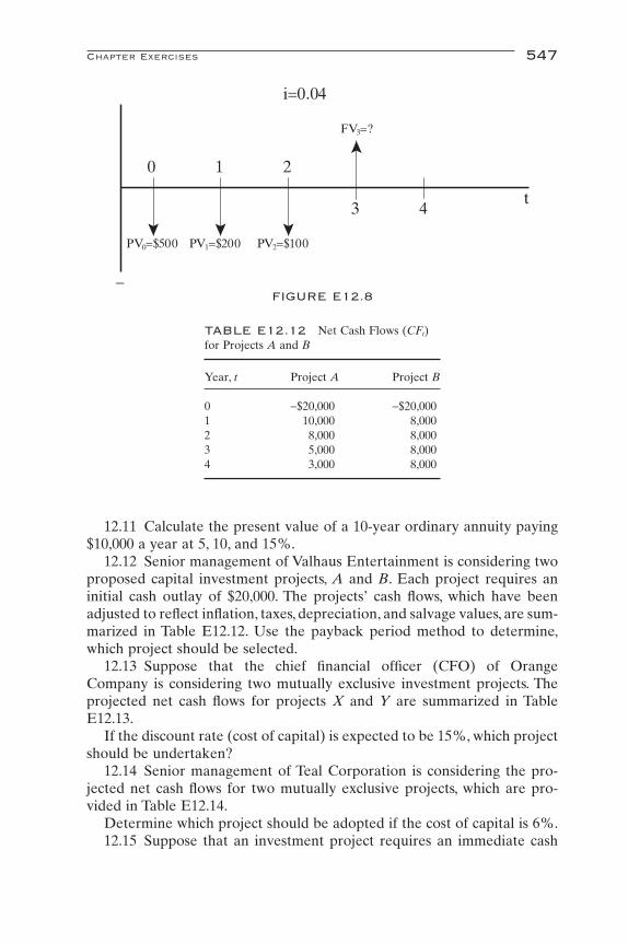
12.11 Calculate the present value of a 10-year ordinary annuity paying$10,000 a year at 5, 10, and 15%.

12.12 Senior management of Valhaus Entertainment is considering twoproposed capital investment projects, A and B. Each project requires aninitial cash outlay of $20,000. The projects’ cash flows, which have beenadjusted to reflect inflation, taxes, depreciation, and salvage values, are sum-marized in Table E12.12. Use the payback period method to determine,which project should be selected.

12.13 Suppose that the chief financial officer (CFO) of OrangeCompany is considering two mutually exclusive investment projects. Theprojected net cash flows for projects X and Y are summarized in TableE12.13.

If the discount rate (cost of capital) is expected to be 15%, which projectshould be undertaken?

12.14 Senior management of Teal Corporation is considering the pro-jected net cash flows for two mutually exclusive projects, which are pro-vided in Table E12.14.

Determine which project should be adopted if the cost of capital is 6%.12.15 Suppose that an investment project requires an immediate cash

Chapter Exercises 547

TABLE E12.12 Net Cash Flows (CFt)for Projects A and B


0 -$20,000 -$20,0001 10,000 8,0002 8,000 8,0003 5,000 8,0004 3,000 8,000

+

–

0 1 2

3 4t

i=0.04

PV0=$500 PV1=$200 PV2=$100

FV3=?

FIGURE E12.8

outlay of $25,000 and provides for an annual cash inflow of $10,000 for thenext 5 years.

a. Estimate the internal rate of return.b. Should the project be undertaken if the cost of capital (hurdle rate)

is 30%?12.16 Illustrate the net present value profile for alternative interest rates

for the cash flow information Projects A and B in Exercise 12.12. Be sureto include in your answer the internal rate of return for each project.

12.17 Red Lion pays a corporate income tax rate of 38%. Red Lion isplanning to build a new factory in the country of Paragon to manufactureprimary and secondary school supplies. The new factory will require animmediate cash outlay of $4 million but is expected to generate annualprofits of $1 million.According to the Paragon Uniform Tax Code, Red Lionmay deduct $250,000 annually as a depreciation expense.The life of the newfactory is expected to be 10 years. Assuming that the annual interest rate is20%, should Red Lion build the new factory? Explain.

12.18 Senior management of Vandaley Enterprises is considering twomutually exclusive investment projects. The projected net cash flows forprojects A and B are summarized in Table E12.18.

If the discount rate (cost of capital) is expected to be 15%, which projectshould be undertaken?


TABLE E12.14 Net Cash Flows forProjects Red and Blue

Year, t Project Red Project Blue

0 -$5,000 -$10,0001 3,000 1,0002 5,500 3,0003 5,0004 7,000

TABLE E12.13 Net Cash Flows forProjects X and Y

Year, t Project X Project Y

0 -$30,000 -$25,0001 10,000 6,0002 12,000 10,0003 14,000 12,0004 15,000 12,0005 8,000 10,000

12.19 Suppose that an investment opportunity, which requires an initial outlay of $100,000, is expected to yield a return of $250,000 after 30years.

a. Will the investment be profitable if the cost of capital is 7%?b. Will the investment be profitable if the cost of capital is 2%?c. At what cost of capital will the investor be indifferent to the

investment?12.20 Consider the net cash flows for Yellow Project given in Table

E12.20.a. What is the net present value profile for Yellow Project at selected

costs of capital?b. Does Yellow Project have multiple internal rate of return? What are

they?c. Diagram your answer.12.21 Calculate the weighted average cost of capital of a project that is

30% debt and 70% equity.Assume that the firm pays 10% on debt and 25%on equity. Assume that the firm’s marginal tax rate is 33%.

SELECTED READINGS

Blank, L. T., and A. J. Tarquin. Engineering Economy, 3rd ed. New York: McGraw-Hill, 1989.Brigham, E. F., and J. F. Houston. Fundamentals of Financial Management, 2nd ed. New York:

Dryden Press, 1999.

Selected Readings 549

TABLE E12.18 Net Cash Flows (CFt)for Projects A and B


0 -$27,000 -$21,0001 8,000 6,5002 9,000 6,5003 10,000 6,5004 10,000 6,5005 6,000 6,500

TABLE E12.20 Net Cash Flows (CFt)for Yellow Project

Year, t CFt

0 -$1,5001 500,0002 -400,000

Brigham, E. F., L. C. Gapenski, and M. C. Erhardt. Financial Management: Theory and Prac-tice, 9th ed. New York: Dryden Press, 1998.

Palm, T., and A. Qayum. Private and Public Investment Analysis. Cincinnati, OH: South-Western Publishing, 1985.

Schall, L. D., and C. W. Haley. Introduction to Financial Analysis, 6th ed. New York: McGraw-Hill, 1991.


Pricing Practices - SU LMS

Documents