On the Pricing of Credit Default Swaps: A Comparative Study between the Reduced-Form Model and the Structural Model Supervisor: Authors: Birger Nilsson Nicklas Ennab Ìvar Grétarsson

Welcome message from author
This document is posted to help you gain knowledge. Please leave a comment to let me know what you think about it! Share it to your friends and learn new things together.
Transcript
On the Pricing of Credit Default Swaps:
A Comparative Study between the Reduced-Form Model and
the Structural Model
Supervisor: Authors:
Birger Nilsson Nicklas Ennab
Ìvar Grétarsson

2
Abstract
This paper focuses on measurement methods of credit risk. By modeling credit
default swap spreads and predicting possible defaults of corporations with the
use of default probabilities this paper makes the search for consistent methods to
measure and manage risk by constructing plausible forecasts of contingent
corporate defaults. The purpose of this paper is to emphasize advantages and
disadvantages of different approaches to measure credit risk. This paper
undertakes the tasks to model credit default swap spreads, using two different
approaches, and to calculate default probabilities. The modeled credit default
spreads are compared to and valued with respect to the market set credit default
swap spreads. By pointing out the relations and differences between the different
models while valuating them this paper will hopefully generate a clear overview
of two different approaches in the contemporary credit risk management and
serve as a guide line for future credit risk management by highlighting the
specific characteristics and outcomes of the different models. Further this paper
considers the credibility in calculated default. Most importantly though this
paper provides a new application to the Hull and White model of pricing a credit
default swap.
Keywords
Credit Risk, Credit Default Swap Spread, The Hull and White Model, The Merton Model,
The Reduced-Form Model, The Structural Model, Probability of Default.

3
Table of Contents
1. Introduction ............................................................................................................................ 4
1.1. Question Formulation ...................................................................................................... 5
1.2. Main Objectives .............................................................................................................. 6
2. Credit Default Swaps ............................................................................................................. 6
3. Theoretical Framework .......................................................................................................... 7
3.1. The Structural Model....................................................................................................... 8
3.1.1. The Merton Model ................................................................................................... 9
3.2. The Reduced-Form Model ............................................................................................ 13
3.2.1. The O´Kane and Turnbull Model ........................................................................... 16
3.2.2. The Applied Hull and White Model ....................................................................... 18
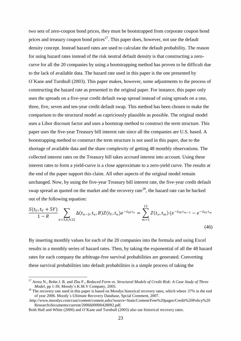
4. Data ...................................................................................................................................... 20
5. Empirical Methodology ........................................................................................................ 21
5.1. Structural Model ............................................................................................................ 22
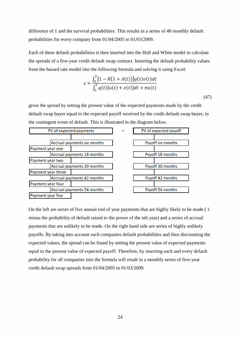
5.2. Reduced-Form Model.................................................................................................... 22
6. Results .................................................................................................................................. 25
7. Conclusion ............................................................................................................................ 30
References ................................................................................................................................ 32
Appendix 1 ............................................................................................................................... 34
Appendix 2 ............................................................................................................................... 44
4
1. Introduction
The importance of the credit derivatives market has grown rapidly over the last years and
revolutionized the trading of credit risk. According to ISDA Mid-Year 2008 Market Survey
the notional amount outstanding of credit derivatives constitutes $62.2 trillion in the
beginning of 2008. The credit derivatives comprise single names, indexes, baskets, and
portfolios of credit default swaps1. Further the ISDA 2009 Derivatives Usage Survey shows
that 94.2 % of the world’s largest companies in the world use derivatives to hedge and
manage risk2. Lately, there have been several innovations in the field of derivatives leading to
new products of managing different mechanisms of business risk that up until recently have
been difficult to isolate and handle properly. The presence of credit derivatives on the market
has shown that there are several advantages to credit derivatives compared to the standard
cash instruments. The use of credit derivatives has shown to be more efficient in sense of
replication in derivative form than the standard form cash instruments. For instance a cash
bond and the repo market can be used to replicate a credit default swap. Further, credit
derivatives have opened up possibilities for new scopes of use. The fields of use includes
hedging credit risk, decreasing concentration of risk in balance sheets and a loosening of
regulatory capital for banks. This is all thanks to the arisen possibility to transfer and leverage
credit risk by the use of credit derivatives3. The development of derivatives during the late
1990s has the character of several dimensions. The classical derivatives such as options and
forwards has risen alongside the dimension of new applications of derivatives use handling
risk beyond the traditional focus on certain parameters like the price and event risk linked to
portfolio risk management and shareholder value among many other. The derivatives use has
also expanded to reach beyond the conventional interest rate, currency, commodity and equity
markets aspects. For example, derivatives have extended to include contemporary
perspectives of inflation and credit. This progress has lead to a significant movement towards
market completion by allowing further breakdown of aggregated business risk by liberating specific
components of risk4. Enabling the transfer of risk from very illiquid credit exposures is perhaps the
most important and significant contribution accomplished by the rise of new credit derivatives. This
paper focuses on measurement methods of credit risk. By modeling credit default swap spreads and
1 International Swaps and Derivatives Association, ISDA News Release, International Swaps and Derivatives
Association Inc, September 24, 2008 2 International Swaps and Derivatives Association, ISDA News Release, International Swaps and Derivatives
Association Inc, April 23, 2009 3 O´Kane D, Credit Derivatives Explained, pp 3-7, Lehman Brothers, 2001
4 Morgan J.P., The J.P. Morgan Guide to Credit Derivatives, pp 7, Risk Publications, 1999
5
predict possible default of corporations with the use of default probabilities this paper makes the
search for consistent methods to measure and manage risk by constructing plausible forecasts of
contingent corporate defaults. Moreover this paper measures risk quantitatively by modeling credit
default swap spreads. Today’s credit risk management literature is disjoined, while the market is in
great need for credit models5. In a study by Jones, Mason and Rosenfeld (1984) it was shown that the
Merton (structural) Model tends to methodically underestimate the observed market set credit default
swap spreads6. In contrast a recent study by Li and Wong (2007) indicates that the structural model
overestimates bond yields. Hence this leads to an overpricing of the market set credit default swap
spread7. In a case study of different models by Arora, Bohn and Zhou (2005) it was reported that the
reduced form model of Hull and White tended to outperform the structural model of Merton8. Hence
there is a necessity for finding a standardized way of measuring and managing credit risk. The purpose
of this paper is to emphasize advantages and disadvantages of different approaches to measure credit
risk. This paper undertakes the tasks to model credit default swap spreads, using two different
approaches, and to calculate default probabilities. The modeled credit default spreads are compared to
and valued with respect to the market set credit default swap spreads. By pointing out the relations and
differences between the different models while valuating them this paper will hopefully generate a
clear overview of two different approaches in the contemporary credit risk management and serve as a
guide line for future credit risk management by highlighting the specific characteristics and outcomes
of the different models. Further this paper considers the credibility in calculated default probabilities.
Most importantly though this paper provides a new application to the Hull and White model of pricing
a credit default swap. By the use of hazard rates to calculate arbitrage free probabilities rather than risk
neutral probabilities used in the original Hull and White model, the authors of this paper intend to
formulate and present a new methodology of pricing credit default swaps.
1.1. Question Formulation
Are the existing reduced form models and structural models in pricing credit default swap
spreads arbitrary?
Which of the two models, prices a credit default swap spread most correctly?
Is the credit default swap spread a plausible quantitative measure of risk?
Can modeling of default probabilities with the use of hazard rates predict the default of
corporate/sovereign entities accurately?
5 O’kane D and Schlögl L, Modeling Credit: Theory and Practice, Lehman Brothers, 2001
6 Jones E.P., Mason S.P., Rosenfeld.E, Contingent Claims Analysis of Corporate Capital Structures: An
Empirical Investigation, Journal of Finance, 39 (1984), pp. 611–625 7 Li K.L., Wong H.Y., Structural Model of Corporate Bond Pricing with Maximum Likelihood Estimation*, pp.
22, Department of Statistics, the Chinese University of Hong Kong, 2007 8 Arora N, Bohn J.R., Zhou F, Reduced Form vs. Structural Models of Credit Risk: A Case A Study of Three
Models, pp.1-39, Moody’s KMV Company, 2005
6
Is the modeled default probability a consistent reliable measure of credit risk?
1.2. Main Objectives
The aim of this paper is to investigate different pricing models of credit default swaps.
Emphasis is put on comparison between the reduced from model to the structural model and
to examine which of the two models that generates the most correct price of credit default
swap spreads. Further, this paper attempts to analyze if default probabilities based on hazard
rates are an arbitrary method to predict default. The intention of this paper is also to determine
to what extent credit default swap prices reflect market anticipation and risk.
2. Credit Default Swaps
The credit default swap can be viewed as a type of derivative security and is an agreement
between the protection buyer and the protection seller. The underlying derivative to the credit
default swap is often bonds or loans. The main idea behind the security is to transfer the
financial loss in an event risk from the protection buyer to the protection seller9, thereby
allowing trade of debt-related credit risk events between market participants. Typically the
protection buyer makes periodic payments called credit swap spreads to the protection seller,
often expressed in basis points per year. In theory, the credit default swap spread would equal
the fixed spread between a floating corporate bond and a floating treasury bond, given that
both are united fixed to a totally riskless rate. However this is not possible in practice. Hence
the credit default swap spread can be approximated to the yield spread between the corporate
bond and the Treasury bond with the same time to maturity and coupon rate as will later be
shown in this paper10
. In the outcome of a credit event in the reference entity (either a
corporation or sovereign issuer) the protection buyer receives a contingent payment from the
protection buyer in return. The difference between the face value of the bond and the market
value of the bond is often what constitutes the contingent amount.
The definition of the credit event is an agreement negotiated by the two counterparties. The
JP Morgan Guide to Credit Derivatives lists the most common credit events that credit default
swaps are associated with, which are:
9 Brigo D, Morini M, CDS Market Formulas and Models, pp 3, 2005
10 Longstaff F, Mithal S, Neis E, The Credit-Default Swap Market: Is Credit Protection Priced Correctly?, USC
FBE Finance Seminar, 2003

7
i) Failure to Meet Payment
ii) Bankruptcy
iii) Repudiation
iv) Material Adverse Structuring of Debt
v) Obligation Acceleration or Obligation Default
One or more of the above mentioned incidents are involved in the settlement of a credit
default swap11
. The maturity of a credit default swap can vary. Since it is traded over the
counter there are possibilities to form the maturity of the credit default swap contract
according to the negotiated settlement of the two counterparties. The five year to maturity
contract is the most widely used on the market of credit default swaps however12
. The
construction of a credit default swap contract is illustrated in the picture below.
Figure 1. Saunders A. and Allen L., Credit Risk Measurement New Approaches to Value at Risk and Other
Paradigms, pp 242, John Wiley & sons, Inc., 2002.
3. Theoretical Framework
Credit risk can be defined as the risk that a borrower will not be able or willing to fulfil its
obligations to the lender, which are to pay the principal on the loan or the interest rates. When
it comes to credit risk modelling there are several contending approaches. The most
commonly used approaches are, however, divided into two alternative methods, the structural
and the reduced-form approach. The structural model relates to models that have the
characteristic of describing the internal structure of the issuer of the debt, so that default is a
consequence of some internal event. These types of models are based on the work of both
11
Morgan J.P., The J.P. Morgan Guide to Credit Derivatives, pp 12-13, Risk Publications, 1999 12
Longstaff F, Mithal S, Neis E, The Credit-Default Swap Market: Is Credit Protection Priced Correctly?, USC
FBE Finance Seminar, 2003
8
Black and Scholes (1973) and Merton (1974). The structural model treats equity as a call
option on the firm’s assets where the strike price is the debt. The model is mainly focusing on
debt valuation. The actual implementation of the model in predicting default gives poor and
negative results, as shown by Jones, Mason and Rosenberg (1984)13
and Jarrow and Van
Deventer (1999)14
. Over the years the model has been extended and implemented by various
researchers, in a try to make different improvements to the model by focusing on additional
theoretical variables15
. Today, however, the Merton model is mostly associated with
predicting the probability of default. In doing so the model treats default as the result of a
company not being able to repay the premium or interest of a loan. As the asset value of a
firm falls below a certain threshold, i.e. the firm’s debt, the firm is considered to be in default.
Structural models can also be used to calculate the appropriate spread on which a corporate
bond should be traded based on the internal structure of the company.
The reduced-form models do not attempt to look at the reasons for the default event. Instead,
the aim of the model is to describe the statistical properties of the default time as accurately as
possible. This is conducted by allowing calculation of the price on fundamental liquid market
instruments and the relative valuation of derivatives16
. The first reduced form model was
presented by Jarrow and Turnbull (1995). To this day, the most widely used reduced form
models are based on the work done by them. In their approach default is predicted by directly
modelling the probability of the default itself. This is achieved by calculating the probability
of default from market prices using a security pricing model17
.
In this section of the paper, the theoretical framework behind the two credit risk models used
to calculate the credit default swap spread in this paper is discussed.
3.1. The Structural Model
The structural model discussed in this part of the paper builds on the groundbreaking work by
Nobel laureate Robert Merton (1974), the Merton model. This paper was the first attempt to
systematically develop a theory of pricing bonds when there is a significant probability of
13
Jones P., Mason S. and Rosenfeld E., Contingent Claims Analysis of Corporate Capital Structure: An
Empirical Investigation, pp 611-625, Journal of Finance, American Finance Association, 1984. 14
Jarrow Robert A. and Van Deventer Donald A. A Practical Usage of Credit Risk Models in Loan Portfolio and
Counterparty Exposure Management, In Credit Risk: Models and Management, Risk Books, 1999.
15 See e.g. Black and Cox (1976), Geske (1977), Vasicek (1984) and Kealhofer (2003). 16
O´Kane D., Schlögl L., Modelling Credit: Theory and Practice, pp. 1-46, Lehman Brothers International
Fixed Income Research, 2001. 17
O´Kane D., Turnbull S., Valuation of Credit Default Swaps, pp. 1-19, Lehman Brothers International Fixed
income Quantitative Credit Research, 2003.
9
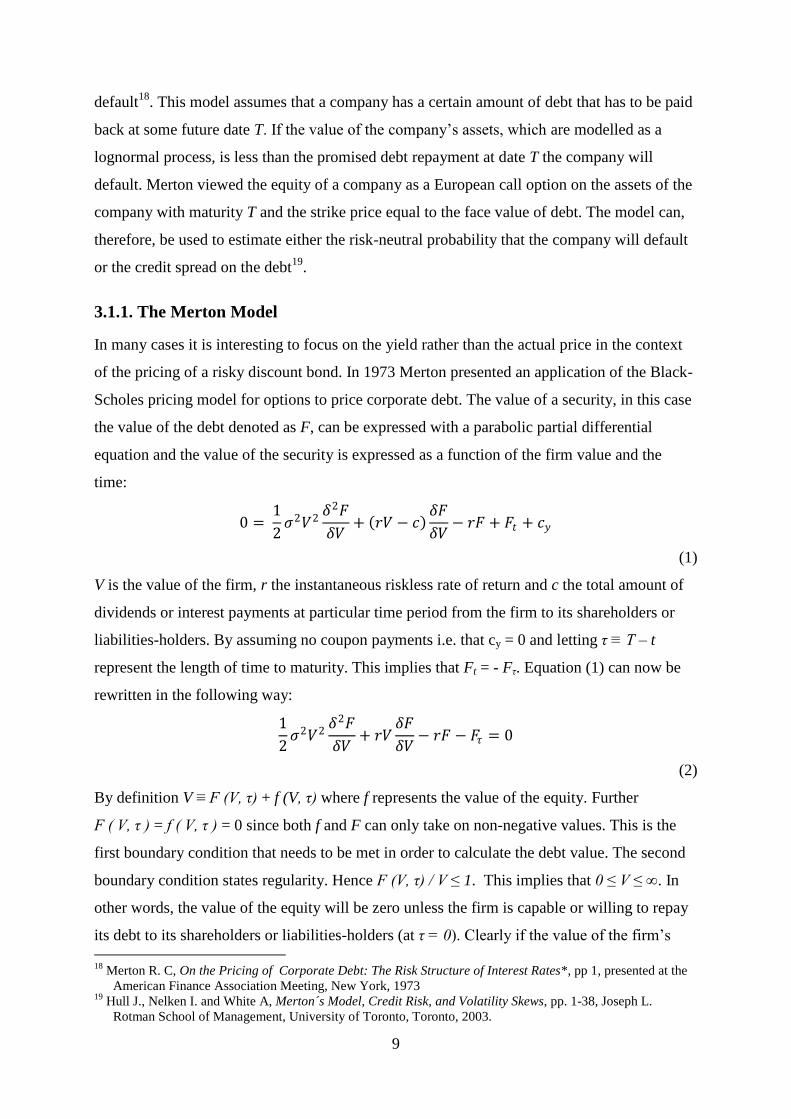
default18
. This model assumes that a company has a certain amount of debt that has to be paid
back at some future date T. If the value of the company’s assets, which are modelled as a
lognormal process, is less than the promised debt repayment at date T the company will
default. Merton viewed the equity of a company as a European call option on the assets of the
company with maturity T and the strike price equal to the face value of debt. The model can,
therefore, be used to estimate either the risk-neutral probability that the company will default
or the credit spread on the debt19
.
3.1.1. The Merton Model
In many cases it is interesting to focus on the yield rather than the actual price in the context
of the pricing of a risky discount bond. In 1973 Merton presented an application of the Black-
Scholes pricing model for options to price corporate debt. The value of a security, in this case
the value of the debt denoted as F, can be expressed with a parabolic partial differential
equation and the value of the security is expressed as a function of the firm value and the
time:
0 = 1
2𝜎2𝑉2
𝛿2𝐹
𝛿𝑉+ 𝑟𝑉 − 𝑐
𝛿𝐹
𝛿𝑉− 𝑟𝐹 + 𝐹𝑡 + 𝑐𝑦
(1)
V is the value of the firm, r the instantaneous riskless rate of return and c the total amount of
dividends or interest payments at particular time period from the firm to its shareholders or
liabilities-holders. By assuming no coupon payments i.e. that cy = 0 and letting τ ≡ Τ – t
represent the length of time to maturity. This implies that Ft = - Fτ. Equation (1) can now be
rewritten in the following way:
1
2𝜎2𝑉2
𝛿2𝐹
𝛿𝑉+ 𝑟𝑉
𝛿𝐹
𝛿𝑉− 𝑟𝐹 − 𝐹𝜏 = 0
(2)
By definition V ≡ F (V, τ) + f (V, τ) where f represents the value of the equity. Further
F ( V, τ ) = f ( V, τ ) = 0 since both f and F can only take on non-negative values. This is the
first boundary condition that needs to be met in order to calculate the debt value. The second
boundary condition states regularity. Hence F (V, τ) / V ≤ 1. This implies that 0 ≤ V ≤ ∞. In
other words, the value of the equity will be zero unless the firm is capable or willing to repay
its debt to its shareholders or liabilities-holders (at τ = 0). Clearly if the value of the firm’s
18
Merton R. C, On the Pricing of Corporate Debt: The Risk Structure of Interest Rates*, pp 1, presented at the
American Finance Association Meeting, New York, 1973 19
Hull J., Nelken I. and White A, Merton´s Model, Credit Risk, and Volatility Skews, pp. 1-38, Joseph L.
Rotman School of Management, University of Toronto, Toronto, 2003.
10
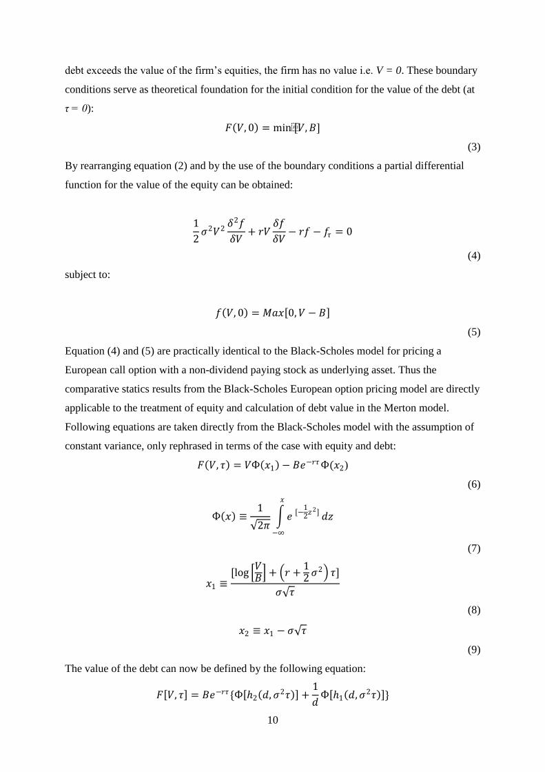
debt exceeds the value of the firm’s equities, the firm has no value i.e. V = 0. These boundary
conditions serve as theoretical foundation for the initial condition for the value of the debt (at
τ = 0):
𝐹 𝑉, 0 = min[𝑉, 𝐵]
(3)
By rearranging equation (2) and by the use of the boundary conditions a partial differential
function for the value of the equity can be obtained:
1
2𝜎2𝑉2
𝛿2𝑓
𝛿𝑉+ 𝑟𝑉
𝛿𝑓
𝛿𝑉− 𝑟𝑓 − 𝑓𝜏 = 0
(4)
subject to:
𝑓 𝑉, 0 = 𝑀𝑎𝑥 0, 𝑉 − 𝐵
(5)
Equation (4) and (5) are practically identical to the Black-Scholes model for pricing a
European call option with a non-dividend paying stock as underlying asset. Thus the
comparative statics results from the Black-Scholes European option pricing model are directly
applicable to the treatment of equity and calculation of debt value in the Merton model.
Following equations are taken directly from the Black-Scholes model with the assumption of
constant variance, only rephrased in terms of the case with equity and debt:
𝐹 𝑉, 𝜏 = 𝑉Ф 𝑥1 − 𝐵𝑒−𝑟𝜏Ф(𝑥2)
(6)
Ф 𝑥 ≡1
2𝜋 𝑒 [−
12𝑧2]
𝑥
−∞
𝑑𝑧
(7)
𝑥1 ≡[log
𝑉𝐵 + 𝑟 +
12 𝜎2 𝜏]
𝜎 𝜏
(8)
𝑥2 ≡ 𝑥1 − 𝜎 𝜏
(9)
The value of the debt can now be defined by the following equation:
𝐹 𝑉, 𝜏 = 𝐵𝑒−𝑟𝜏 {Ф 2 𝑑, 𝜎2𝜏 +1
𝑑Ф 1 𝑑, 𝜎2𝜏 }
11
(10)
where
𝑑 ≡𝐵𝑒−𝑟𝜏
𝑉
(11)
1 𝑑, 𝜎2𝜏 ≡ −[12 𝜎2𝜏 − log 𝑑 ]
𝜎 𝜏
(12)
2 𝑑, 𝜎2𝜏 ≡ −[12 𝜎2𝜏 + log 𝑑 ]
𝜎 𝜏
(13)
Finally equation (10) is rearranged to be expressed in terms of yields rather than actual values:
𝑅 𝜏 − 𝑟 = −1
𝜏𝑙𝑜𝑔{Ф 2 𝑑, 𝜎2𝜏 +
1
𝑑Ф 1 𝑑, 𝜎2𝜏 }
(14)
having in mind that
𝑒−𝑅(𝜏)𝜏 ≡𝐹 𝑉, 𝜏
𝐵
(15)
which is given from equation (11)20
. Equation (14) is a straightforward hands-on expression
for convenient calculation procedures. The Merton model is very practical to apply in many
cases regarding different kinds of derivative instruments.
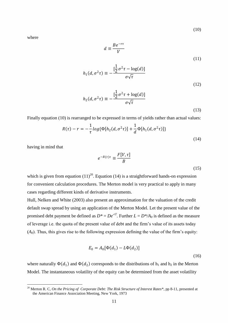
Hull, Nelken and White (2003) also present an approximation for the valuation of the credit
default swap spread by using an application of the Merton Model. Let the present value of the
promised debt payment be defined as D* = De-rT
. Further L = D*/A0 is defined as the measure
of leverage i.e. the quota of the present value of debt and the firm’s value of its assets today
(A0). Thus, this gives rise to the following expression defining the value of the firm’s equity:
𝐸0 = 𝐴0[Ф 𝑑1 − 𝐿Ф 𝑑2 ]
(16)
where naturally Ф 𝑑1 and Ф 𝑑2 corresponds to the distributions of h1 and h2 in the Merton
Model. The instantaneous volatility of the equity can be determined from the asset volatility
20
Merton R. C, On the Pricing of Corporate Debt: The Risk Structure of Interest Rates*, pp 8-11, presented at
the American Finance Association Meeting, New York, 1973

12
by the use of diffusion processes. Hull, Nelken and White uses Itô’s Lemma to express the
instantaneous volatility of the equity in terms of the asset volatility and the measure of
leverage:
𝜎𝐸 =𝜎𝐴Ф(𝑑1)
Ф 𝑑1 − 𝐿Ф(𝑑2)
(17)
The equation is reached from the following expression combined with equation (16):
𝐸0𝜎𝐸 =𝜕𝐸
𝜕𝐴𝐴0𝜎𝐴
(18)
The arbitrage free probability that the firm will default at time T is given by:
𝜆 = Ф(−𝑑2)
The leverage L, the asset volatility σ and the time to repayment T are the parameters
determining the arbitrage free probability for default. The implied credit spread on a risky
debt can now be explained from this. Set:
𝐵0 = 𝐴0 − 𝐸0
(19)
Incorporating equation (16) into this expression gives:
𝐵0 = 𝐴0[Ф −𝑑1 + 𝐿Ф 𝑑2 ]
(20)
From the definition D*=De-rT
, B0 can be rephrased as:
𝐵0 = 𝐷𝑒−𝑦𝑇 = 𝐷∗𝑒 𝑟−𝑦 𝑇
(21)
Employing equation (21) and by the use of A0 = D*/L:
𝑦 = 𝑟 − ln Ф 𝑑2 +Ф −𝑑1
𝐿 /𝑇
(22)
By some rearrangement the expression for the implied credit spread can be formulated:
𝑠 = 𝑦 − 𝑟 = − ln Ф 𝑑2 +Ф −𝑑1
𝐿 /𝑇
(23)
13
3.2. The Reduced-Form Model
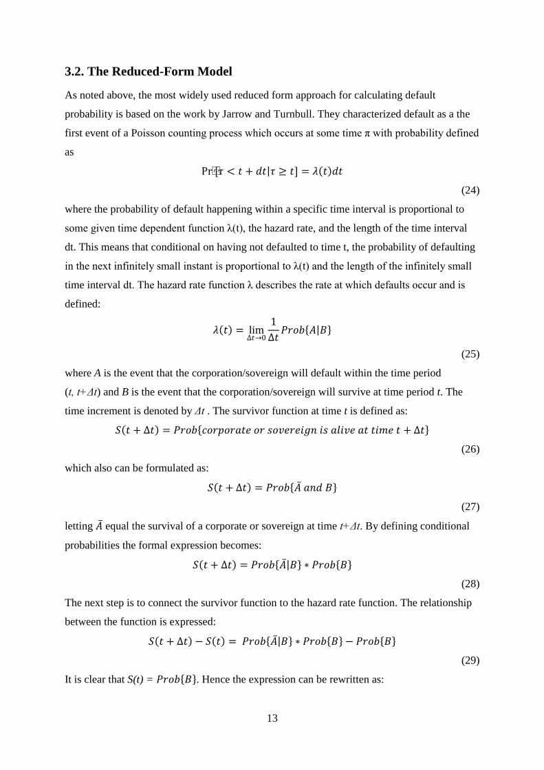
As noted above, the most widely used reduced form approach for calculating default
probability is based on the work by Jarrow and Turnbull. They characterized default as a the
first event of a Poisson counting process which occurs at some time π with probability defined
as
Pr[𝜏 < 𝑡 + 𝑑𝑡 𝜏 ≥ 𝑡] = 𝜆 𝑡 𝑑𝑡
(24)
where the probability of default happening within a specific time interval is proportional to
some given time dependent function λ(t), the hazard rate, and the length of the time interval
dt. This means that conditional on having not defaulted to time t, the probability of defaulting
in the next infinitely small instant is proportional to λ(t) and the length of the infinitely small
time interval dt. The hazard rate function λ describes the rate at which defaults occur and is
defined:
𝜆 𝑡 = lim∆𝑡→0
1
∆𝑡𝑃𝑟𝑜𝑏 𝐴 𝐵
(25)
where A is the event that the corporation/sovereign will default within the time period
(t, t+Δt) and B is the event that the corporation/sovereign will survive at time period t. The
time increment is denoted by Δt . The survivor function at time t is defined as:
𝑆 𝑡 + ∆𝑡 = 𝑃𝑟𝑜𝑏 𝑐𝑜𝑟𝑝𝑜𝑟𝑎𝑡𝑒 𝑜𝑟 𝑠𝑜𝑣𝑒𝑟𝑒𝑖𝑔𝑛 𝑖𝑠 𝑎𝑙𝑖𝑣𝑒 𝑎𝑡 𝑡𝑖𝑚𝑒 𝑡 + ∆𝑡
(26)
which also can be formulated as:
𝑆 𝑡 + ∆𝑡 = 𝑃𝑟𝑜𝑏 𝐴 𝑎𝑛𝑑 𝐵
(27)
letting 𝐴 equal the survival of a corporate or sovereign at time t+Δt. By defining conditional
probabilities the formal expression becomes:
𝑆 𝑡 + ∆𝑡 = 𝑃𝑟𝑜𝑏 𝐴 𝐵 ∗ 𝑃𝑟𝑜𝑏 𝐵
(28)
The next step is to connect the survivor function to the hazard rate function. The relationship
between the function is expressed:
𝑆 𝑡 + ∆𝑡 − 𝑆 𝑡 = 𝑃𝑟𝑜𝑏 𝐴 𝐵 ∗ 𝑃𝑟𝑜𝑏 𝐵 − 𝑃𝑟𝑜𝑏 𝐵
(29)
It is clear that S(t) = 𝑃𝑟𝑜𝑏 𝐵 . Hence the expression can be rewritten as:
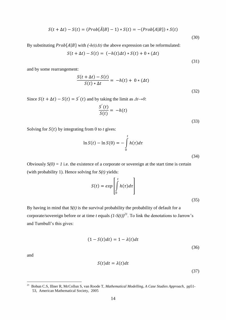
14
𝑆 𝑡 + ∆𝑡 − 𝑆 𝑡 = 𝑃𝑟𝑜𝑏 𝐴 𝐵 − 1 ∗ 𝑆 𝑡 = − 𝑃𝑟𝑜𝑏 𝐴 𝐵 ∗ 𝑆 𝑡
(30)
By substituting 𝑃𝑟𝑜𝑏 𝐴 𝐵 with (-h(t)Δt) the above expression can be reformulated:
𝑆 𝑡 + ∆𝑡 − 𝑆 𝑡 = − 𝑡 𝛥𝑡 ∗ 𝑆 𝑡 + 0 ∗ (𝛥𝑡)
(31)
and by some rearrangement:
𝑆 𝑡 + ∆𝑡 − 𝑆 𝑡
𝑆 𝑡 ∗ ∆𝑡= − 𝑡 + 0 ∗ (𝛥𝑡)
(32)
Since 𝑆 𝑡 + ∆𝑡 − 𝑆 𝑡 = 𝑆′(𝑡) and by taking the limit as Δt→0:
𝑆′(𝑡)
𝑆(𝑡)= −(𝑡)
(33)
Solving for 𝑆(𝑡) by integrating from 0 to t gives:
ln 𝑆 𝑡 − ln 𝑆(0) = − 𝜏 𝑑𝜏
𝑡
0
(34)
Obviously S(0) = 1 i.e. the existence of a corporate or sovereign at the start time is certain
(with probability 1). Hence solving for S(t) yields:
𝑆 𝑡 = 𝑒𝑥𝑝 𝜏 𝑑𝜏
𝑡
0
(35)
By having in mind that S(t) is the survival probability the probability of default for a
corporate/sovereign before or at time t equals (1-S(t))21
. To link the denotations to Jarrow’s
and Turnbull’s this gives:
1 − 𝑆 𝑡 𝑑𝑡 = 1 − 𝜆 𝑡 𝑑𝑡
(36)
and
𝑆 𝑡 𝑑𝑡 = 𝜆 𝑡 𝑑𝑡
(37)
21
Bohun C.S, Illner R, McCollun S, van Roode T, Mathematical Modelling, A Case Studies Approach, pp51-
53, American Mathematical Society, 2005

15
Jarrow and Turnbull model default using a simple two period model. Extending this model to
multiple time periods it can easily be seen how they modelled default using a binomial tree, as
shown below:
A company will either survive with the probability 1-λ(t)dt or default with the probability
being λ(t)dt. If the company defaults it will receive a payoff of K which is the recovery rate.
The reduced-form model discussed in this part of the paper is the one presented by Hull and
White in 2000. However, instead of using the default density concept introdcued by Hull and
White this paper uses a hazard rate for the default probability. The hazard rate used in this
paper is the one presented by O´Kane and Turnbull in 2003. Therefore, first the O´Kane and
Turnbull model will be discussed and then the Hull and White model.
Figure 2. O´Kane D. and Turnbull S, Valuation of Credit Default Swaps, pp. 1-19, Lehman
Brothers International Fixed income Quantitative Credit Research, 2003.
16
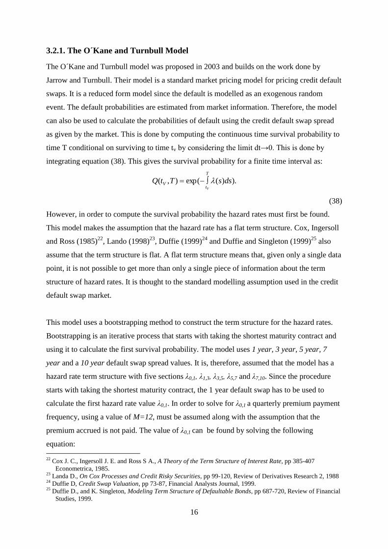
3.2.1. The O´Kane and Turnbull Model
The O´Kane and Turnbull model was proposed in 2003 and builds on the work done by
Jarrow and Turnbull. Their model is a standard market pricing model for pricing credit default
swaps. It is a reduced form model since the default is modelled as an exogenous random
event. The default probabilities are estimated from market information. Therefore, the model
can also be used to calculate the probabilities of default using the credit default swap spread
as given by the market. This is done by computing the continuous time survival probability to
time T conditional on surviving to time tv by considering the limit dt→0. This is done by
integrating equation (38). This gives the survival probability for a finite time interval as:
).)(exp(),( dssTtQT
tV
V
(38)
However, in order to compute the survival probability the hazard rates must first be found.
This model makes the assumption that the hazard rate has a flat term structure. Cox, Ingersoll
and Ross (1985)22
, Lando (1998)23
, Duffie (1999)24
and Duffie and Singleton (1999)25
also
assume that the term structure is flat. A flat term structure means that, given only a single data
point, it is not possible to get more than only a single piece of information about the term
structure of hazard rates. It is thought to the standard modelling assumption used in the credit
default swap market.
This model uses a bootstrapping method to construct the term structure for the hazard rates.
Bootstrapping is an iterative process that starts with taking the shortest maturity contract and
using it to calculate the first survival probability. The model uses 1 year, 3 year, 5 year, 7
year and a 10 year default swap spread values. It is, therefore, assumed that the model has a
hazard rate term structure with five sections λ0,1, λ1,3, λ3,5, λ5,7 and λ7,10. Since the procedure
starts with taking the shortest maturity contract, the 1 year default swap has to be used to
calculate the first hazard rate value λ0,1. In order to solve for λ0,1 a quarterly premium payment
frequency, using a value of M=12, must be assumed along with the assumption that the
premium accrued is not paid. The value of λ0,1 can be found by solving the following
equation:
22
Cox J. C., Ingersoll J. E. and Ross S A., A Theory of the Term Structure of Interest Rate, pp 385-407
Econometrica, 1985. 23
Landa D., On Cox Processes and Credit Risky Securities, pp 99-120, Review of Derivatives Research 2, 1988 24
Duffie D, Credit Swap Valuation, pp 73-87, Financial Analysts Journal, 1999. 25
Duffie D., and K. Singleton, Modeling Term Structure of Defaultable Bonds, pp 687-720, Review of Financial
Studies, 1999.
17
12,9,6,3
33
12
1
1
),(),(),(),,(
),(),(),()1(
)1,(
n
nvnVnVnn
m
mVmVmV
VVttQttQttZBtt
ttQttQttZR
YttS
(39)
where
S(tv,tv+ 1Y) is the one year credit default swap spread quoted on the market.
Δ(tn-3,tn,B) is the day count fraction between premium dates tn-3 and tn in the
appropriate basis convention denoted by B.
Q(tv,T) is the arbitrage-free survival probability.
Z(tv,T) is the Libor discount factor. The model makes the assumption that users have
been able to bootstrap a full term structure of Libor discount factors in the currency of
the default swap being priced.
R is the recovery rate. The model uses historical recovery rates.
The upper part of this equation is known as the present value of the protection leg while the
lower part is the present value of the premium leg. The protection leg is the contingent
payment of (100% - R) on the face value of the protection made following a default. The
premium leg is the series of payments of the default swap spread made to maturity or to the
time of default, whichever happens first.
In order to solve the equation above the model uses a one-dimensional root-searching
algorithm and the fact that Q(tv,T)=Σexp(-λ(t)τm). The following equation can now be solved
to find the value of λ0,1:
12,9,6,3
12
1
3 ))(,(),(),,(1
)1,(0110101
n m
mvnVnnVV mmn eettZettZBtt
R
YttS
(40)
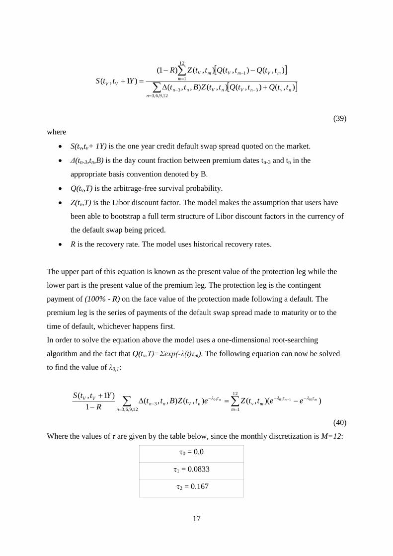
Where the values of τ are given by the table below, since the monthly discretization is M=12:
τ0 = 0.0
τ1 = 0.0833
τ2 = 0.167
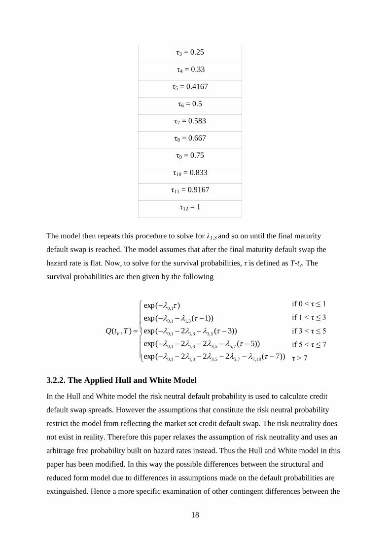
18
τ3 = 0.25
τ4 = 0.33
τ5 = 0.4167
τ6 = 0.5
τ7 = 0.583
τ8 = 0.667
τ9 = 0.75
τ10 = 0.833
τ11 = 0.9167
τ12 = 1
The model then repeats this procedure to solve for λ1,3 and so on until the final maturity
default swap is reached. The model assumes that after the final maturity default swap the
hazard rate is flat. Now, to solve for the survival probabilities, τ is defined as T-tv. The
survival probabilities are then given by the following
if 0 < τ ≤ 1
if 1 < τ ≤ 3
if 3 < τ ≤ 5
if 5 < τ ≤ 7
τ > 7
3.2.2. The Applied Hull and White Model
In the Hull and White model the risk neutral default probability is used to calculate credit
default swap spreads. However the assumptions that constitute the risk neutral probability
restrict the model from reflecting the market set credit default swap. The risk neutrality does
not exist in reality. Therefore this paper relaxes the assumption of risk neutrality and uses an
arbitrage free probability built on hazard rates instead. Thus the Hull and White model in this
paper has been modified. In this way the possible differences between the structural and
reduced form model due to differences in assumptions made on the default probabilities are
extinguished. Hence a more specific examination of other contingent differences between the
))7(222exp(
))5(22exp(
))3(2exp(
))1(exp(
)exp(
),(
10,77,55,33,11,0
7,55,33,11,0
5,33,11,0
3,11,0
1,0
TtQ V

19
two models is enabled. Except from this deviation, this paper replicates the Hull and White
model to price the credit default swap spreads. Several parameters are used in the modelling
of the credit default swap spreads and are defined as follows:
T: Life time of the credit default swap
h(t): The arbitrage free probability intensity at time t.
R: Moody’s average recovery rates for bonds i.e. the reference obligation to the credit default
swaps in the Hull and White model.
u(t): Present value of payments between time 0 and t at the rate of $1 per year.
e(t): Present value of an accrual payment at time t. Note that it equals t-t* where the instant
payment date preceding time t is denoted by t*.
v(t): Present value of $1 at time t.
ω: The aggregated payments per year made by the credit default swap buyer.
s: The value of the total payments per year ω that makes the value of the credit default swap
equal to zero.
1-λ: The arbitrage free probability that no credit event will occur during the life time of the
credit default swap.
A(t): Accrued interest in percent of face value on the reference obligation ( here the reference
obligation is a senior bond) at time t.
Given that a credit event occurs at time t (t<T) the present value of the payments is
ω[u(t)+e(t)]. However if no credit event occurs during the time to maturity of the contract
then the present value of the payments at time T is ωu(T). This implies that the expected
present value of the payments is:
𝜔 𝜆 𝑡 𝑢 𝑡 + 𝑒 𝑡 𝑑𝑡 + 1 − 𝜆 𝜔
𝑇
0
𝑢(𝑇)
(41)
Further the arbitrage free expected payoff from the credit default swap is:
1 − 1 + 𝐴 𝑡 𝑅 = 1 − 𝑅 − 𝐴(𝑡)𝑅
(42)
Thus the present value of the arbitrage free expected payoff from the credit default swap is
defined:
[1 − 𝑅 − 𝐴(𝑡)𝑅
𝑇
0
]𝜆 𝑡 𝑣 𝑡 𝑑𝑡
(43)
20
By subtracting the expected present value of the payments from the present value of the
arbitrage free expected payoff the value of the credit default swap is attained:
[1 − 𝑅 − 𝐴(𝑡)𝑅
𝑇
0
]𝜆 𝑡 𝑣 𝑡 𝑑𝑡 − 𝜔 𝜆 𝑡 𝑢 𝑡 + 𝑒 𝑡 𝑑𝑡 + 1 − 𝜆 𝜔
𝑇
0
𝑢(𝑇)
(44)
The credit default swap spread, denoted by s, is the value of 𝜔 that induces the expression to
become equal to zero:
𝑠 = [1 − 𝑅 − 𝐴(𝑡)𝑅
𝑇
0]𝜆 𝑡 𝑣 𝑡 𝑑𝑡
𝜆 𝑡 𝑢 𝑡 + 𝑒 𝑡 𝑑𝑡 + 1 − 𝜆 𝑇
0𝑢(𝑇)
(45)
The variable s is the total payments per year in percentage form of the notional principal for a
newly issued credit default swap26
.
4. Data
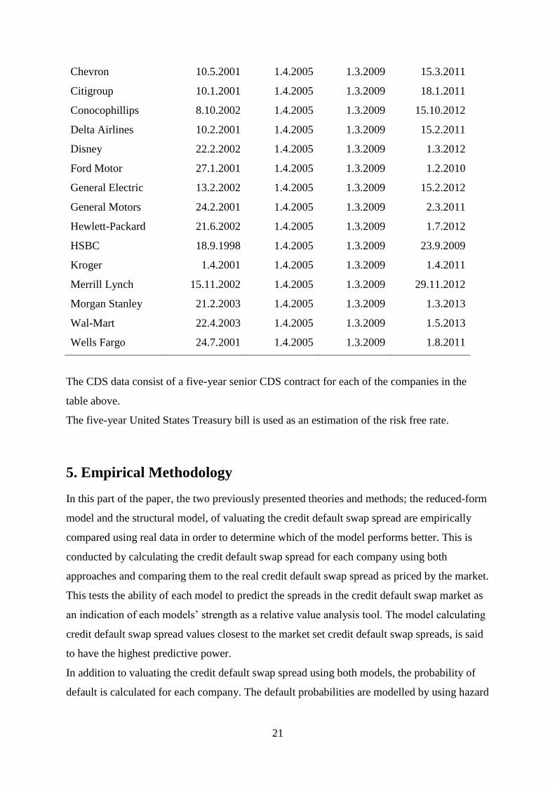
This section of the thesis offers a presentation on the data used in this paper. All data was
collected from the DataStream database and consist of the yield to maturity on corporate
bonds and data on actual credit default swap spreads together with the interest rate of the
United States five-year Treasury bill. The data include prices quoted monthly from
01/04/2005 to 01/03/2009. Values were picked the first weekday of each month which results
in 48 observations.
Only US dollar-denominated corporate bonds were selected in order to get the yield to
maturity. Information about the bonds is presented in the table below.
Starting date First date Last date Last
Company of data presented presented date of data
AIG 8.5.2003 1.4.2005 1.3.2009 15.5.2013
Bear Stearns 31.10.2002 1.4.2005 1.3.2009 15.11.2014
Berkshire Hathaway 15.12.2003 1.4.2005 1.3.2009 15.12.2010
Boeing 2.11.2001 1.4.2005 1.3.2009 15.2.2012
Caterpillar 6.8.2003 1.4.2005 1.3.2009 13.8.2010
26
Hull J, White A, Valuing Credit Default Swaps I: No Counterparty Default Risk, pp. 13-14, Joseph L. Rotman
School of Management, University of Toronto, Toronto, 2000.
21
Chevron 10.5.2001 1.4.2005 1.3.2009 15.3.2011
Citigroup 10.1.2001 1.4.2005 1.3.2009 18.1.2011
Conocophillips 8.10.2002 1.4.2005 1.3.2009 15.10.2012
Delta Airlines 10.2.2001 1.4.2005 1.3.2009 15.2.2011
Disney 22.2.2002 1.4.2005 1.3.2009 1.3.2012
Ford Motor 27.1.2001 1.4.2005 1.3.2009 1.2.2010
General Electric 13.2.2002 1.4.2005 1.3.2009 15.2.2012
General Motors 24.2.2001 1.4.2005 1.3.2009 2.3.2011
Hewlett-Packard 21.6.2002 1.4.2005 1.3.2009 1.7.2012
HSBC 18.9.1998 1.4.2005 1.3.2009 23.9.2009
Kroger 1.4.2001 1.4.2005 1.3.2009 1.4.2011
Merrill Lynch 15.11.2002 1.4.2005 1.3.2009 29.11.2012
Morgan Stanley 21.2.2003 1.4.2005 1.3.2009 1.3.2013
Wal-Mart 22.4.2003 1.4.2005 1.3.2009 1.5.2013
Wells Fargo 24.7.2001 1.4.2005 1.3.2009 1.8.2011
The CDS data consist of a five-year senior CDS contract for each of the companies in the
table above.
The five-year United States Treasury bill is used as an estimation of the risk free rate.
5. Empirical Methodology
In this part of the paper, the two previously presented theories and methods; the reduced-form
model and the structural model, of valuating the credit default swap spread are empirically
compared using real data in order to determine which of the model performs better. This is
conducted by calculating the credit default swap spread for each company using both
approaches and comparing them to the real credit default swap spread as priced by the market.
This tests the ability of each model to predict the spreads in the credit default swap market as
an indication of each models’ strength as a relative value analysis tool. The model calculating
credit default swap spread values closest to the market set credit default swap spreads, is said
to have the highest predictive power.
In addition to valuating the credit default swap spread using both models, the probability of
default is calculated for each company. The default probabilities are modelled by using hazard

22
rates. The results for both the credit default swap spreads and default probabilities are
presented in graphical form in the appendix at the end of this paper.
5.1. Structural Model
According to theory the five-year credit default swap spread is very close to the credit spread
of the yield on a five-year corporate bond over a yield on a five-year bond issued by the
government. This is the approximated credit spread implied by Merton (s = y - r)
In order to solve for the credit default swap spread, denoted s, the yields of a five-year
corporate bond and a five-year government bond need to be collected. For the government
bond yields, the interest rates on a five-year Treasury bill are chosen. The interest rate in the
beginning of each month is picked over a study period from 01/04/2005 to 01/03/2009 which
results in 48 observations. The yields of the corporate bonds are, however, not as clear. Data
on five-year corporate bonds is in extensively short supply. In order to solve for the yields of
a five-year corporate bond interpolation is used. Interpolation is a method of approximating a
yield that is unknown using yields that are known. It is the process of determining an
unknown point that lies between two known points. The unknown point being the yield on a
five-year bond while the known points being yields on bonds with shorter and longer time to
maturity respectively. In this paper, linear interpolation is used as a methologdy of guessing
what the value of the unknown yield is. A number of corporate bonds were chosen for each
company and by interpolation a yield-curve on five-year corporate bond was constructed with
observations ranging from the same study period as the collected interest rates on the
government bond. All in all 48 observations were picked for each corporate bond and the
government bonds. Then it is just a simple matter of taking the difference between corporate
bond yields and the interest rate on the five-year Treasury bill for each of the 20 chosen
corporations. This results in a monthly series of 48 five-year credit default swap spreads for
each company using the structural model.
5.2. Reduced-Form Model
The reduced-form model used to calculate the credit default swap spread in this paper is an
application of the model presented by Hull and White (2000). The original model incorporates
the default density concept, which is the unconditional cumulative default probability within
one period, disregarding contingent events in other time periods. This model generates default
densities recursively based on a set of both zero-coupon corporate bond prices and zero-
coupon Treasury bond prices, and by assuming an expected recovery rate. In order to get the
23
two sets of zero-coupon bond prices, they must be bootstrapped from corporate coupon bond
prices and treasury coupon bond prices27
. This paper does, however, not use the default
density concept. Instead hazard rates are used to calculate the default probability. The reason
for using hazard rates instead of the risk neutral default density is that constructing a zero-
curve for all the 20 companies by using a bootstrapping method has proven to be difficult due
to the lack of available data. The hazard rate used in this paper is the one presented by
O´Kane and Turnbull (2003). This paper makes, however, some adjustments to the process of
constructing the hazard rate as presented in the original paper. For instance, this paper only
uses the spreads on a five-year credit default swap spread instead of using spreads on a one,
three, five, seven and ten-year credit default swap. This method has been chosen to make the
comparison to the structural model as capriciously plausible as possible. The original model
uses a Libor discount factor and uses a bootstrap method to construct the term structure. This
paper uses the five-year Treasury bill interest rate since all the companies are U.S. based. A
bootstrapping method to construct the term structure is not used in this paper, due to the
shortage of available data and the share complexity of getting 48 monthly observations. The
collected interest rates on the Treasury bill takes accrued interest into account. Using these
interest rates to form a yield-curve is a close approximate to a zero-yield curve. The results at
the end of the paper support this claim. All other aspects of the original model remain
unchanged. Now, by using the five-year Treasury bill interest rate, the five-year credit default
swap spread as quoted on the market and the recovery rate28
, the hazard rate can be backed
out of the following equation:
𝑆(𝑡𝑉 , 𝑡𝑉 + 5𝑌)
1 − 𝑅 ∆ 𝑡𝑛−3, 𝑡𝑛 , 𝐵 𝑍(𝑡𝑉 ,
𝑛=3,6,9,12
𝑡𝑛)𝑒−𝜆05𝜏𝑛 = 𝑍 𝑡𝑣 , 𝑡𝑚
12
𝑚=1
(𝑒−𝜆05𝜏𝑚−1 − 𝑒−𝜆01𝜏𝑚
(46)
By inserting monthly values for each of the 20 companies into the formula and using Excel
results in a monthly series of hazard rates. Then, by taking the exponential of all the 48 hazard
rates for each company the arbitrage-free survival probabilities are generated. Converting
these survival probabilities into default probabilities is a simple process of taking the
27
Arora N., Bohn J. R. and Zhu F., Reduced Form vs. Structural Models of Credit Risk: A Case Study of Three
Model, pp 1-39, Moody´s K.M.V Company, 2005. 28
The recovery rate used in this paper is based on Moodys historical recovery rates, which where 37% in the end
of year 2006. Moody´s Ultimate Recovery Database, Spcial Comment, 2007.
.http://www.moodys.com/cust/content/content.ashx?source=StaticContent/Free%20pages/Credit%20Policy%20
Research/documents/current/2006600000428092.pdf.
Both Hull and White (2000) and O´Kane and Turnbull (2003) also use historical recovery rates.
24
difference of 1 and the survival probabilities. This results in a series of 48 monthly default
probabilities for every company from 01/04/2005 to 01/03/2009.
Each of these default probabilities is then inserted into the Hull and White model to calculate
the spreads of a five-year credit default swap contract. Inserting the default probability values
from the hazard rate model into the following formula and solving it using Excel:
𝑠 = 1 − 𝑅 1 + 𝐴 𝑡 𝑞 𝑡 𝑣 𝑡 𝑑𝑡
𝑇
0
𝑞 𝑡 𝑢 𝑡 + 𝑒 𝑡 𝑑𝑡 + 𝜋𝑢(𝑡)𝑇
0
(47)
gives the spread by setting the present value of the expected payments made by the credit
default swap buyer equal to the expected payoff received by the credit default swap buyer, in
the contingent event of default. This is illustrated in the diagram below.
On the left are series of five annual end of year payments that are highly likely to be made ( 1
minus the probability of default raised to the power of the nth year) and a series of accrual
payments that are unlikely to be made. On the right hand side are series of highly unlikely
payoffs. By taking into account each companies default probabilities and then discounting the
expected values, the spread can be found by setting the present value of expected payments
equal to the present value of expected payoff. Therefore, by inserting each and every default
probability for all companies into the formula will result in a monthly series of five-year
credit default swap spreads from 01/04/2005 to 01/03/2009.

25
6. Results
This paper has investigated all in all 20 corporations. Starting off in alphabetic order, the
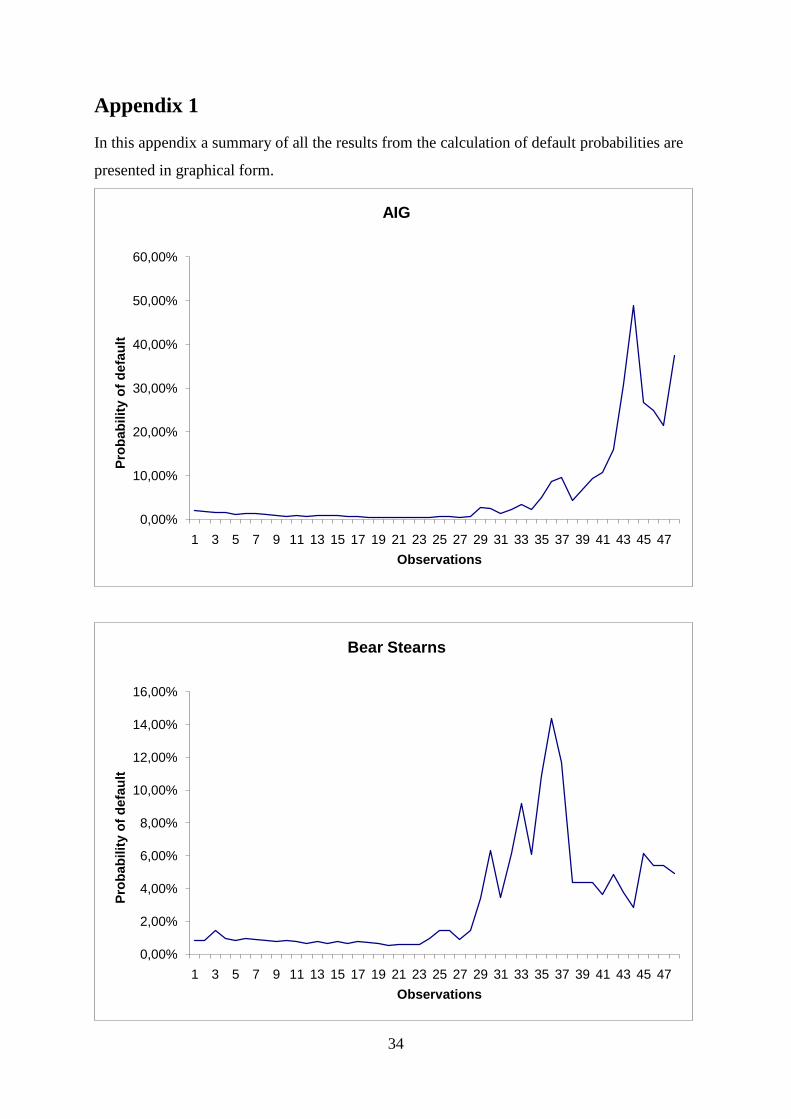
probability of default for AIG during the first 27 months of the studied time period was close
to zero with an average around 1,5 %. After 27 months a rapid increase in the probability of
default occurs and reaches its peak on the 45th
month of the observed time period with a
default probability as high as almost 50 %. The growth of the credit default swap spread
shows the same kind of development. From staying at a relatively constant level at around
0,01 the market credit default swap spread rises to 0,25 from the 27th
month to the 45th
.
Eventually AIG defaulted. The reduced and structural modelled credit default swap spreads
lay close to the market set credit default swap spread during the periods of low values. In the
time periods characterized by increased riskiness (after the 27th
observation until the 48th
and
last observation) the modelled credit default swap spreads deviated somewhat from the
market set credit default swap spread with a tendency to overestimate the value of the credit
default swap spread.
Bear Sterns also shows a dramatic increase in the default probability after the 27th
observation. From being stable with an approximate 1% risk of default the probability of the
default grows to 15 % in the 37th
observation. It decreases then fast to an approximate average
of 4% for the remaining observations. The same pattern can be gathered in the value of the
credit default swap spread for Bear Sterns. At an initial level at 0,002 lasting up until the 27th
observation it goes up to over 0,03 in the 37th
observation and then falls down to an average
of 0,01 for the last observations. One should have in mind that Bear Sterns received a loan
from the Federal Reserve Bank of New York during the chaotic months in the beginning of
the financial crisis in an attempt to avoid default. To no avail Bear Sterns was later sold to JP
Morgan Chase for a very low price. The new ownership is reflected in the levels of default
probability and credit default swap spread. Where the AIG default probability and credit
default swap spread continued to rise up until the 45th
observation, Bear Sterns probability of
default and credit default swap spread fell down again after the purchase of the company,
implying a lower risk for default and increased credibility when taken under the wings of JP
Morgan Chase. The modelled credit default swap spreads for Bear Sterns deviates extensively
from the market set credit default swap spread. In particular the structural model
overestimates the market set credit default swap spread remarkably much. It is worth pointing
out that both the modelled credit default swap spreads did not reflect the break point with the
same magnitude as the market set credit default swap spread and default probability with the
26
JP Morgan Chase purchase of the company. The modelled credit default swap spread
overestimates the market set value even more after the break point. The reduced and structural
modelled credit default swap spreads are increasingly volatile after the break point. In general
the structural model overestimates the value of the credit default swap spread more than the
reduced form model for Bear Sterns.
Berkshire Hathaway, a company operating in the property and casualty insurance industry
mainly, has it highest noted default probability, barely over 20%, in the 48th
observation. In
the same sample period the credit default swap spread is at maximum 0,05. The structural
model tends to underestimate the value of the market set credit default swap spread for the
last third of the observations while the reduced form model overestimates the value
throughout all observations.
The result for the air line company Boeing indicates that the risk for default did not start to
increase until the 34th
month with a peak value after 47 months reaching a level nearly over
14%. The same goes for the value of the credit default swap spread. Compared to previous
companies’ results the crisis trend appears later in time. There might be a logical explanation
to this since the recession started out as a financial crisis where banks and other financial
institutes experienced dramatic losses which later on downpour to other business sectors.
Hence the lagged effect of increasing default probabilities and credit default swap spreads has
a plausible explanation. Once again the structural model appears to overestimate the credit
default swap spread value more than the reduced form model and shows also a more volatile
pattern. The market set credit default swap spread is at highest close to 0,03. Caterpillar is
another company in a sector, not involved in the financial business sector, namely
manufacturing of construction and mining equipment mainly. The trend is the same as for
Boeing. The tendencies of recession with dramatic rises in probability of default and
consequently the credit default swap spread appear later on. Around the 34th
month both the
default probability and the credit default swap spread increases fast up to levels of 16% and a
value nearly under 0,04 respectively in the 48th
and last observation. Once again the structural
model seems to overestimate the credit default swap spread more in general.
The trend of overestimated modelled credit default swap spreads is obvious when looking at
car manufacturer Chevron. Here the structural model clearly overestimates the market set
credit default swap spread throughout the whole observation period. Meanwhile the reduced
form model performs better and lies within a close distance to the market set credit default
swap spread which has the highest value at 0,01 in the 45th
observation. This includes
reasonably that the default probability is the lowest for all the companies discussed yet. The
27
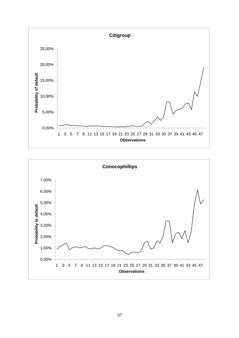
maximum probability of default for Chevron ended up being barely over 6%. Citigroup is a
major American financial service corporation. The default probability for the company shows
like most other companies within the financial sector a clear increment in the default
probability after the 27th
observation. Even though Citigroup was bailed out by the American
Government in November 2008, remarkably the trend of fast growing default probability and
increasing credit default swap spread values kept on. The highest values of default probability
is 18% in the 48th
observation and credit default swap value of 0,05 roundabout. This could
mean that a government bailout does not always imply a shift towards more positive
anticipation of the future of the company. On the other hand it is quite impossible to
determine whether the default probability and the credit default swap spread of Citigroup
would have risen even more without the government bailout. The structural model performs
once again poorer than the reduced form model, both overestimating the market set credit
default swap spread.
The huge energy corporation ConocoPhillips seems not have been struck so hard by the
financial crisis compared to many other large corporations. The top value of default
probability is around 6% in the 46th
observation and the highest measured credit default swap
spread value is about 0,01. Still there is a rise in both the default probability and the credit
default swap spread due to the effect of recession. Moreover it follows the same outline in the
observation as other non-financial corporations. The risk measurement values increase
somewhat later than for the financial corporations. Yet again the reduced form model
performs better than the structural model.
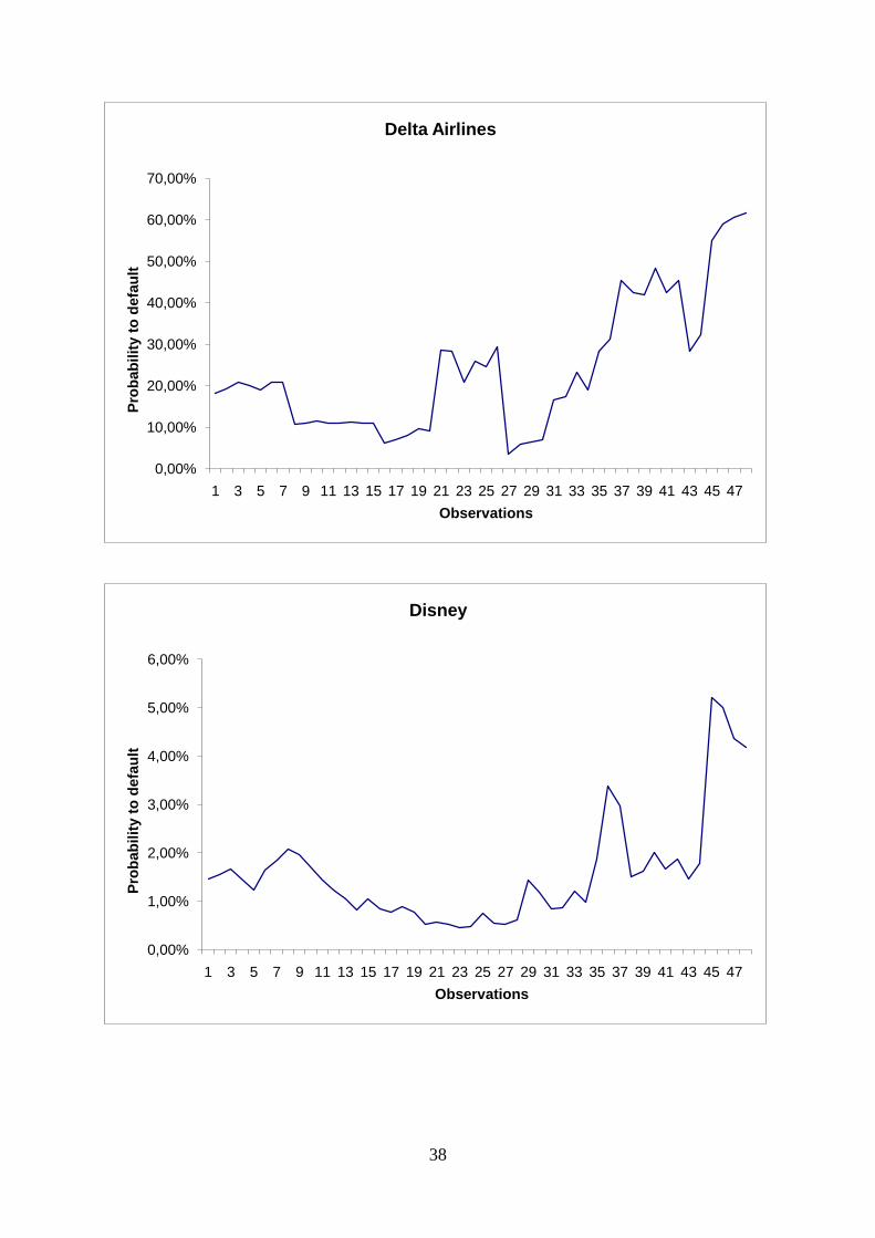
The situation for Delta Airlines differs substantially than for the other non-financial sector
corporations. The company shows an overall high probability for default over the whole
studied time period and in the last and 48th
observation in march 2009 the modelled
probability of default for Delta Airlines was above 60%. Consequently the credit default swap
spread value for the company rose to 0,2 which is considered to be a very high value. Despite
these tremendous indications of default Delta Airlines is still operating. However the result is
strange. The modelled credit default swap spreads are expected to correlate positively to both
the market set credit default swap spread and to the default probability. However for the
structured from model, it’s the opposite in this case, which rises some concern over either the
collected data or the calculations. The structural model starts out at a sky high credit default
swap spread value and then decreases significantly in contrast to both the market set credit
default swap spread and the reduced form modelled credit default swap spread as well as the
default probability. Since the reduced form model performs as expected and both the reduced

28
and structural models are based on the same default probability, the cause of error must lie in
another endogenously given variable.
Moving on to Disney, based in the entertainment industry, both the credit swaps spread value
and the default probability indicates small increases in risk due to the recession and compared
to many other companies the impact of the recession has not been very extensive. The 46th
observation gives the highest default probability, which is 5,5% and in the same time period
the credit default swap spread value is at its highest, 0,011. Both the modelled credit default
swap spreads are more volatile than the market set credit default swap spread and as in earlier
cases overestimated.
For Ford Motor the situation has been very precarious which the results are showing. The 44th
observation gives an over 70% probability of default and the credit default swap spread
For the 44th
observation is over 0,3. It is very unsure if Ford Motors will survive the recession
due to the alarming indications of default.
General Electric on the other hand is not concerned with default to the same extent as Ford
Motors but still shows some considerable effects of the recession with a default probability
peaking at the 48th
observation at 30% and a credit default swap spread value of 0,08 at most.
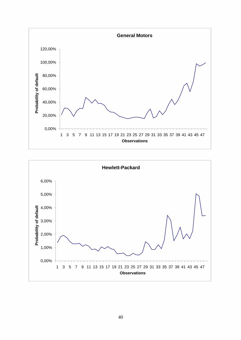
The default probabilities and credit default swap spreads for General Motors are remarkable.
The default probability is close to 100% for the last observations and the credit default swap
spreads at 1,4. For the moment General Motors is undergoing bankruptcy reorganization
according to Chapter 1129
. According to the results this is hardly surprising. Worth
mentioning is that the modelled credit default swap spreads using the structural model is
surprisingly underestimating the market set value throughout all observations. Both models
are underestimating the market set credit default swap spreads for the last four observations
i.e. observation 45 to 48. This result stands in sharp contrast to previous observations.
However one should bear in mind that the case of General Motors is extreme.
Hewlett-Packard is a technology corporation mainly manufacturing computing. The results
for the company indicate only a small effect of the recession. Default probability tops at the
45th
month at approximately 5%. Meanwhile the credit default swap spread value peaks at
barely above 0,01. These results must be interpreted in the context of today’s economical
environment. Hence the numbers for Hewlett-Packard points towards a relatively stable
survival probability given nothing unexpected happens that would dramatically change the
29
US courts, Bankruptcy Basics Chapter 11,
http://www.uscourts.gov/bankruptcycourts/bankruptcybasics/chapter11.html
29
situation for the company. As before the structural form model tends to overestimate the
market set credit default swap spread more than the reduced form model.
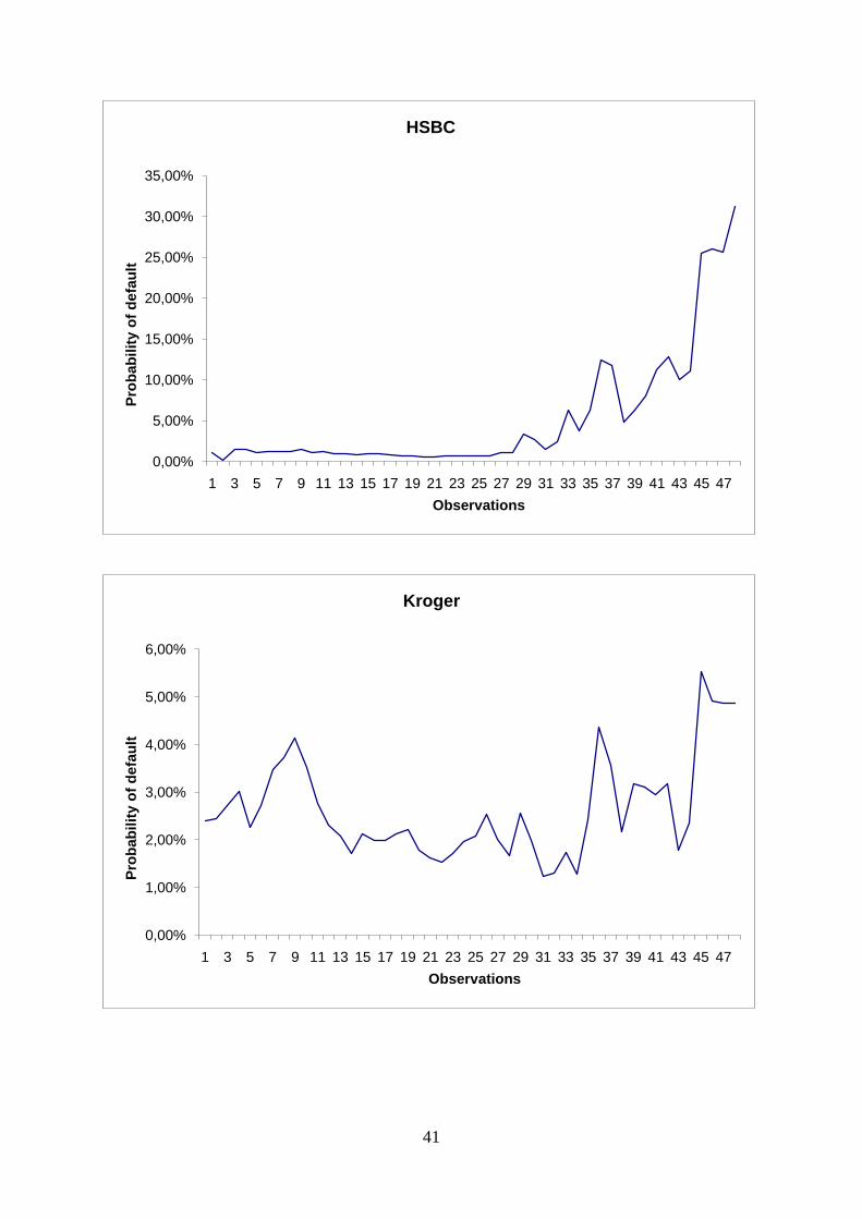
As the world’s largest banking group HSBC Holdings shows results that goes in line with
many of the other financial corporations’ under study in this paper. With a top default
probability in the 48th
month with a fast growing default probability from the 27th
month with
corresponding credit default swap spread values increases at the same time peaking at a level
of 0,085 in the 48th
observation, it is clear that also HSBC Holdings has carried great risk
during the financial crisis.
The large American retail supermarket chain Kroger Co is relatively unaffected by the
recession according to the results. With an average around 3% default probability over the
whole study period the top notation is reached at the 45th
observation with 5,5%. In the same
observation period the credit default swap spread reaches the maximum of the study period
with a value of 0,01. Still the structural model outnumbers the reduced form model in
overestimation of the market set credit default swap spread.
In January 2009 the Bank of America acquired Merrill Lynch, a global financial service
corporation based in the United States, in order to calm down the negative anticipations of the
financial crisis and to avoid Merrill Lynch from default. This acquisition was already
announced in September 2008. Apparently the effect of the acquisition was successful. The
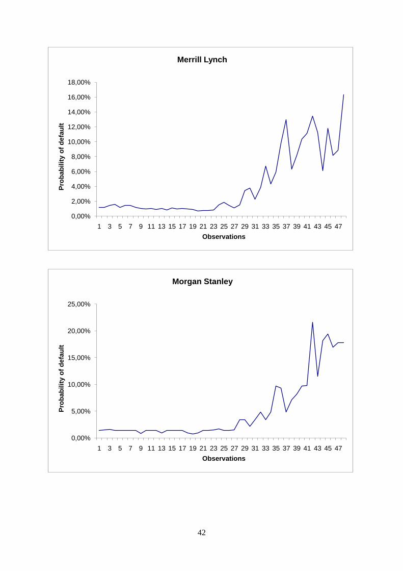
default probability of Merrill Lynch is assuredly high but not like for AIG for instance. The
top noted default probability is in the 48th
observation at a level of about 16%. Surprisingly
the highest record for the credit default swap spread, 0,04, is noted in the 43rd
observation.
Morgan Stanley is another global financial service corporation in the United States. The
default probability culminates at 22% in the 43rd
observation. Meanwhile the credit default
swap spread peaks at approximately 0,09. In September 2008 Mitsubishi UFJ Financial Group
bought 21% of Morgan Stanley. During this time period Morgan Stanley announced the
transition from being an investment bank to a customary bank holding company. These two
aspects might have winded down some of the stressful anticipations of the future of Morgan
Stanley. Thus the contributions of these events have led to the decrease in default probability
and hence the credit default swap spread values over the last couple of months in the
observation period.
Wal-Mart is a corporation running large department stores in the United States. By a view of
the results it is quite obvious that the impact of the financial crisis and the following recession
has been limited. The default probability is at most 5,5% in the 46th
observation and the
highest credit default swap spread value, 0,01, is noted in the 45th
observation.
30
Wells Fargo & Co is a financial services company that has been considered being very stable.
With a maximum 10,5% default probability in the last and 48th
observation and a credit
default swap spread reaching 0,025 in the last observation Wells Fargo & Co remains
relatively stable.
7. Conclusion
Generally it can be concluded that high default probabilities are directly related to actual
defaults. There is a substantial evidence of a positive correlation. However, the default
probability should only be considered as an indication of default rather than a definite
determinant of actual default. For instance, the default probabilities for AIG and General
Motors clearly indicated a high probability of default. Eventually both companies did default.
On the other hand some companies like General Electric who had a high probability of default
did not default and are actually doing well at the moment. An explanation to the high default
probabilities for companies that are not in financial distress can be attributed the ongoing
financial crisis which has led to an unsure economic environment turning up the general risk
level in the world economy. The impact of the financial crisis has been largest on the
companies within the financial sector. Companies operating in non-financial sectors have not
been affected to the same extent by the present crisis. All in all it can be said that the default
probability is a plausible measure of credit risk.
In the pricing of the credit default swap spreads it turns out that the reduced-form model
outperforms the structural model in almost every observation. This is clear evidence of the
empirical superiority of the reduced-form model. It is definitely more accurate in pricing the
credit default swap spread and is therefore considered to be more consistent and reliable than
the structural model. It is more suitable as an analysis tool. In line with the findings of Li and
Wong (2007) the structural model tends to overestimate the market set credit default swap
spread. However, the reduced-form model also overestimates the market set credit default
swap spread but not to the same extent. This raises the question whether the market is capable
of pricing credit default swap spreads correctly. As discussed earlier there are no standardized
methods to price credit default swap spreads. Perhaps the market set credit default swap
spread reflects this disunity. Since both the reduced-form and structural model use bonds as
reference obligation there is a huge risk of information incompleteness. Bonds are in general
relatively illiquid. Thus, bond yields tend to react slower to changes in the economic

31
environment. However, this concern can probably be disregarded since the modelled credit
default swap spreads closely positively correlated to the market credit default swap spread and
not showing any signs of lagging. Another possible reason for the modelled credit default
swap spread overshooting is the high volatility characterizing the economy for the moment.
This study shows that under low risk, i.e. low volatility, in the economy the models perform
well, showing signs of consistency. During time periods of high volatility the models tend to
perform worse.
This study reflects the great concern of finding a standardized and consistent method of
pricing credit default swap spreads. This study has also shown that contemporary models of
pricing credit default swap spreads are not entirely reliable and should be interpreted
cautiously. Since trading with credit default swaps has grown rapidly over the last few years
further studies on the subject are necessary.

32
References
Arora N, Bohn J.R., Zhou F, Reduced Form vs. Structural Models of Credit Risk: A Case A
Study of Three Models, pp. 1-39, Moody’s KMV Company, 2005.
Black, F., & Cox, J., Valuing Corporate Securities: Some Effects of Bond Indenture
Provisions, pp. 351-367Journal of Finance, 31, 1976.
Bohun C.S, Illner R, McCollun S, van Roode T, Mathematical Modelling, A Case Studies
Approach, pp. 51-53, American Mathematical Society, 2005.
Brigo D, Morini M, CDS Market Formulas and Models, pp 3, 2005.
Geske, R., The Valuation of Corporate Liabilities as Compound Options, pp. 541-552 Journal
of Financial and Quantitative Analysis, 1977.
Hull J., Nelken I. and White A, Merton´s Model, Credit Risk, and Volatility Skews, pp. 1-38,
Joseph L. Rotman School of Management, University of Toronto, Toronto, 2003.
Hull J, White A, Valuing Credit Default Swaps I: No Counterparty Default Risk, pp. 13-14,
Joseph L. Rotman School of Management, University of Toronto, Toronto, 2000.
International Swaps and Derivatives Association, ISDA News Release, International Swaps
and Derivatives Association Inc, April 23, 2009.
International Swaps and Derivatives Association, ISDA News Release, International Swaps
and Derivatives Association Inc, September 24, 2008.
Jarrow Robert A. and Van Deventer Donald A. A Practical Usage of Credit Risk Models in
Loan Portfolio and Counterparty Exposure Management, In Credit Risk: Models and
Management, Risk Books, 1999.
Jones E.P., Mason S.P., Rosenfeld.E, Contingent Claims Analysis of Corporate Capital
Structures: An Empirical Investigation, pp. 611-625, Journal of Finance, 39, 1984.
33
Li K.L., Wong H.Y., Structural Model of Corporate Bond Pricing with Maximum Likelihood
Estimation*, pp. 22, Department of Statistics, the Chinese University of Hong Kong, 2007.
Longstaff F, Mithal S, Neis E, The Credit-Default Swap Market: Is Credit Protection Priced
Correctly?, USC FBE Finance Seminar, 2003.
Merton R. C, On the Pricing of Corporate Debt: The Risk Structure of Interest Rates*, pp 1,
8-11, presented at the American Finance Association Meeting, New York, 1973.
Moody´s Ultimate Recovery Database, Spcial Comment, 2007.
http://www.moodys.com/cust/content/content.ashx?source=StaticContent/Free%20pages/Cre
dit%20Policy%20Research/documents/current/2006600000428092.pdf.
Morgan J.P., The J.P. Morgan Guide to Credit Derivatives, pp 7, Risk Publications, 1999.
O´Kane D, Credit Derivatives Explained, pp 3-7, Lehman Brothers, 2001.
O´Kane D., Schlögl L., Modelling Credit: Theory and Practice, pp. 1-46, Lehman Brothers
International Fixed Income Research, 2001.
O´Kane D., Turnbull S., Valuation of Credit Default Swaps, pp. 1-19, Lehman Brothers
International Fixed income Quantitative Credit Research, 2003.
Saunders, A., & Allen, L., Credit Risk Measurement - New Approaches to Value at Risk and
Other Paradigms, Second Edition. John Wiley & Sons, Inc., 2002.
US courts, Bankruptcy Basics Chapter 11,
http://www.uscourts.gov/bankruptcycourts/bankruptcybasics/chapter11.html
Vasicek, O. A., Credit Valuation - White Paper. MoodysKMV corporation, 1984.
34
Appendix 1
In this appendix a summary of all the results from the calculation of default probabilities are
presented in graphical form.
0,00%
10,00%
20,00%
30,00%
40,00%
50,00%
60,00%
1 3 5 7 9 11 13 15 17 19 21 23 25 27 29 31 33 35 37 39 41 43 45 47
Pro
bab
ilit
y o
f d
efa
ult
Observations
AIG
0,00%
2,00%
4,00%
6,00%
8,00%
10,00%
12,00%
14,00%
16,00%
1 3 5 7 9 11 13 15 17 19 21 23 25 27 29 31 33 35 37 39 41 43 45 47
Pro
bab
ilit
y o
f d
efa
ult
Observations
Bear Stearns

35
0,00%
5,00%
10,00%
15,00%
20,00%
25,00%
1 3 5 7 9 11 13 15 17 19 21 23 25 27 29 31 33 35 37 39 41 43 45 47
Pro
bab
ilit
y o
f d
efa
ult
Observations
Berkshire Hathaway
0,00%
2,00%
4,00%
6,00%
8,00%
10,00%
12,00%
14,00%
16,00%
1 3 5 7 9 11 13 15 17 19 21 23 25 27 29 31 33 35 37 39 41 43 45 47
Pro
bab
ilit
y o
f d
efa
ult
Observations
Boeing

36
0,00%
2,00%
4,00%
6,00%
8,00%
10,00%
12,00%
14,00%
16,00%
18,00%
1 3 5 7 9 11 13 15 17 19 21 23 25 27 29 31 33 35 37 39 41 43 45 47
Pro
bab
ilit
y o
f d
efa
ult
Observations
Caterpillar
0,00%
1,00%
2,00%
3,00%
4,00%
5,00%
6,00%
7,00%
1 3 5 7 9 11 13 15 17 19 21 23 25 27 29 31 33 35 37 39 41 43 45 47
Pro
bab
ilit
y t
o d
efa
ult
Observations
Chevron
37
0,00%
5,00%
10,00%
15,00%
20,00%
25,00%
1 3 5 7 9 11 13 15 17 19 21 23 25 27 29 31 33 35 37 39 41 43 45 47
Pro
bab
ilit
y o
f d
efa
ult
Observations
Citigroup
0,00%
1,00%
2,00%
3,00%
4,00%
5,00%
6,00%
7,00%
1 3 5 7 9 11 13 15 17 19 21 23 25 27 29 31 33 35 37 39 41 43 45 47
Pro
bab
ilit
y t
o d
efa
ult
Observations
Conocophillips
38
0,00%
10,00%
20,00%
30,00%
40,00%
50,00%
60,00%
70,00%
1 3 5 7 9 11 13 15 17 19 21 23 25 27 29 31 33 35 37 39 41 43 45 47
Pro
bab
ilit
y t
o d
efa
ult
Observations
Delta Airlines
0,00%
1,00%
2,00%
3,00%
4,00%
5,00%
6,00%
1 3 5 7 9 11 13 15 17 19 21 23 25 27 29 31 33 35 37 39 41 43 45 47
Pro
bab
ilit
y t
o d
efa
ult
Observations
Disney

39
0,00%
10,00%
20,00%
30,00%
40,00%
50,00%
60,00%
70,00%
80,00%
1 3 5 7 9 11 13 15 17 19 21 23 25 27 29 31 33 35 37 39 41 43 45 47
Pro
bab
ilit
y o
f d
efa
ult
Observations
Ford Motor
0,00%
5,00%
10,00%
15,00%
20,00%
25,00%
30,00%
35,00%
1 3 5 7 9 11 13 15 17 19 21 23 25 27 29 31 33 35 37 39 41 43 45 47
Pro
bab
ilit
y o
f d
efa
ult
Observations
General Electric
40
0,00%
20,00%
40,00%
60,00%
80,00%
100,00%
120,00%
1 3 5 7 9 11 13 15 17 19 21 23 25 27 29 31 33 35 37 39 41 43 45 47
Pro
bab
ilit
y o
f d
efa
ult
Observations
General Motors
0,00%
1,00%
2,00%
3,00%
4,00%
5,00%
6,00%
1 3 5 7 9 11 13 15 17 19 21 23 25 27 29 31 33 35 37 39 41 43 45 47
Pro
bab
ilit
y o
f d
efa
ult
Observations
Hewlett-Packard
41
0,00%
5,00%
10,00%
15,00%
20,00%
25,00%
30,00%
35,00%
1 3 5 7 9 11 13 15 17 19 21 23 25 27 29 31 33 35 37 39 41 43 45 47
Pro
bab
ilit
y o
f d
efa
ult
Observations
HSBC
0,00%
1,00%
2,00%
3,00%
4,00%
5,00%
6,00%
1 3 5 7 9 11 13 15 17 19 21 23 25 27 29 31 33 35 37 39 41 43 45 47
Pro
bab
ilit
y o
f d
efa
ult
Observations
Kroger
42
0,00%
2,00%
4,00%
6,00%
8,00%
10,00%
12,00%
14,00%
16,00%
18,00%
1 3 5 7 9 11 13 15 17 19 21 23 25 27 29 31 33 35 37 39 41 43 45 47
Pro
bab
ilit
y o
f d
efa
ult
Observations
Merrill Lynch
0,00%
5,00%
10,00%
15,00%
20,00%
25,00%
1 3 5 7 9 11 13 15 17 19 21 23 25 27 29 31 33 35 37 39 41 43 45 47
Pro
bab
ilit
y o
f d
efa
ult
Observations
Morgan Stanley

43
0,00%
1,00%
2,00%
3,00%
4,00%
5,00%
6,00%
1 3 5 7 9 11 13 15 17 19 21 23 25 27 29 31 33 35 37 39 41 43 45 47
Pro
bab
ilit
y o
f d
efa
ult
Observations
Wal-Mart
0,00%
2,00%
4,00%
6,00%
8,00%
10,00%
12,00%
1 3 5 7 9 11 13 15 17 19 21 23 25 27 29 31 33 35 37 39 41 43 45 47
Pro
bab
ilit
y o
f d
efa
ult
Observations
Wells Fargo

44
Appendix 2
In this appendix a summary of all the results from the calculation of the credit default swap
spreads are presented in graphical form. The diagrams show the spreads for both the structural
model and the reduced-form model along with the actual spreads as priced by the market.

45
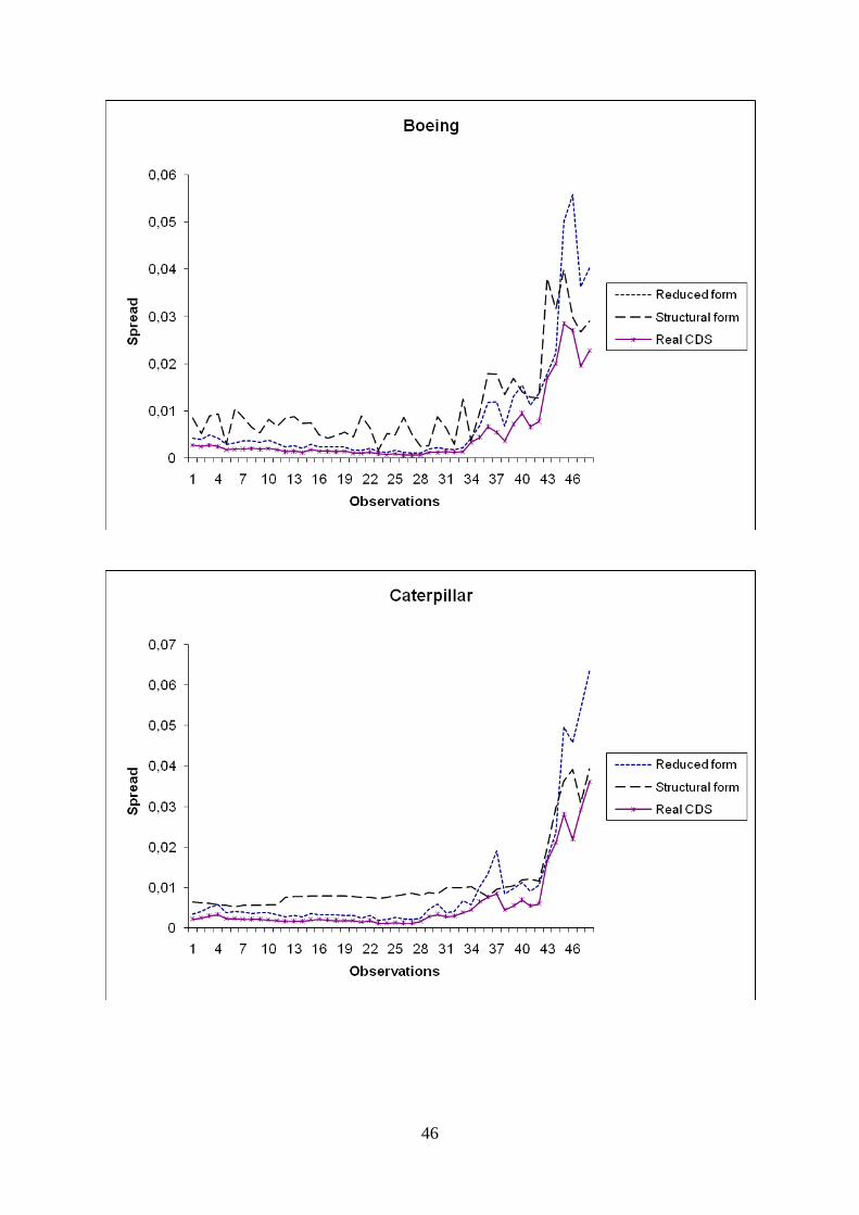
46
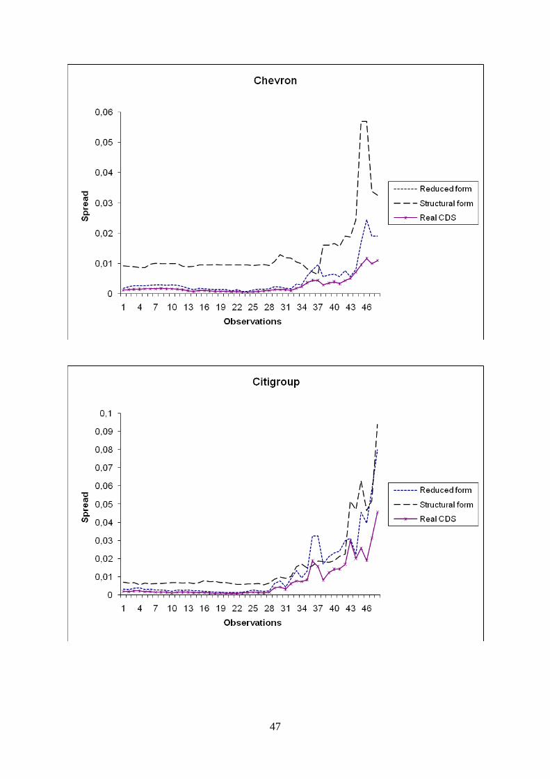
47
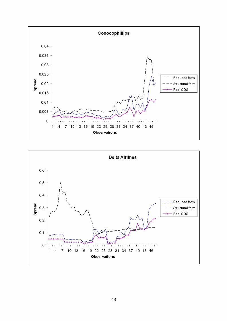
48

49
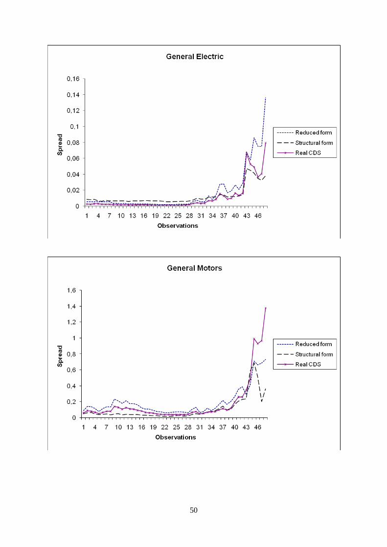
50

51
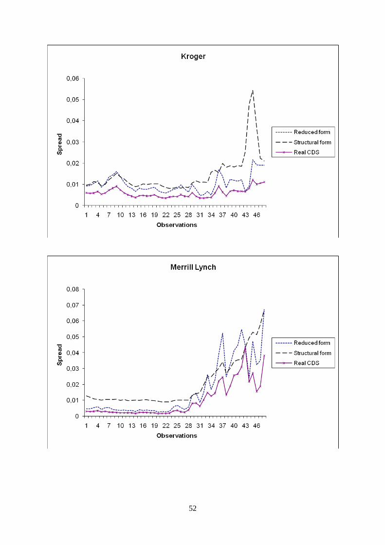
52

53
0
0,005
0,01
0,015
0,02
0,025
0,03
1 4 7 10 13 16 19 22 25 28 31 34 37 40 43 46
Sp
read
Observations
Wal-Mart
Reduced form
Structural form
Real CDS
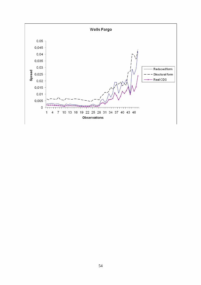
54

55
Related Documents