Pricing-based Spectrum Access Control in Cognitive Radio …informationnet.asu.edu/pub/CRN_pricing.pdf · 2010-08-01 · Pricing-based Spectrum Access Control in Cognitive Radio Networks

Pricing-based Spectrum Access Control inCognitive Radio Networks with Random Access

Lei Yang∗, Hongseok Kim†, Junshan Zhang∗, Mung Chiang‡, and Chee Wei Tan§∗School of Electrical, Computer and Energy Engineering, Arizona State University, Tempe, AZ, 85287

†Bell Labs, Alcatel-Lucent, Murray Hill, NJ, 07974‡Department of Electrical Engineering, Princeton University, Princeton, NJ, 08544

§City University of Hong Kong, 83 Tat Chee Avenue, Kowloon Hong Kong

Abstract—Market-based mechanisms are promising ap-proaches for spectrum access in cognitive radio networks. Inthis paper, we focus on two market models, one with a monopolyprimary user (PU) market and the other with a multiple PUmarket, where each PU sells its temporarily unused spectrum tosecondary users (SUs). We propose a pricing-based spectrumtrading mechanism that enables SUs to contend for channelusage by random access, in a distributed manner, which inturn mitigates the complexity and time overhead associated withcentralized scheduling. For the monopoly PU market model, westart with SUs contending via slotted Aloha. The revenue maxi-mization problems here are nonconvex. Observing that the globaloptimal pricing strategy is Pareto optimal, we first characterizethe Pareto optimal region, and then obtain a Pareto optimalsolution that maximizes the SUs’ throughput subject to the SUs’budget constraints. To mitigate the spectrum underutilization dueto “price of contention,” we revisit the problem where SUs contentvia CSMA. Spectrum utilization is enhanced, resulting in higherrevenue. When the PU’s unused spectrum is a control parameter,we study further the tradeoff between the PU’s utility and itsrevenue.

Next, for the multiple PU market model, we cast the com-petition among PUs as a three-stage Stackelberg game, whereeach SU selects a PU’s channel to maximize its throughput. Wecharacterize the Stackelberg equilibria, in terms of access pricesand the spectrum offered to SUs. Our findings reveal that thenumber of equilibria has a threshold structure: if the numberof PUs is greater than the threshold, there exist infinitely manyequilibria; otherwise, there exists a unique equilibrium, wherethe access prices and spectrum opportunities are determined bythe budgets/elasticity of SUs and the utility level of PUs.

I. INTRODUCTION

Cognitive radio (CR) is expected to capture temporal andspatial “spectrum holes” in the spectrum white space, andto enable spectrum sharing for secondary users (SUs). Onechallenge is that SUs should be able to discover spectrumholes and access them efficiently and fairly, without causinginterference to the primary users (PUs), especially when thedemand for available spectrum nearly outstrips the supply.

Market-based mechanisms have been explored as an im-portant approach for spectrum access. Among these mecha-nisms, auction-based spectrum access mechanisms have beenextensively studied for different objectives, e.g., incentivecompatibility [1]–[4], spectrum reuse [1], [2], [5], [6], auction-eer’s revenue maximization [2], social welfare maximization[6], power allocation schemes for the SUs with interferenceprotection for the PU [7], etc. These works mainly focus on

on-demand auctions where each SU requests spectrum basedon its traffic demand, and the time overhead can be signifi-cant in the auction procedure. Compared with auction-basedspectrum access mechanisms, pricing-based spectrum accessmechanisms may incur lower time overhead (see [8]–[14] andthe references herein). Among these approaches, [8] studiedpricing policies for a PU to sell unused spectrum to multipleSUs by using stochastic dynamic programming. [9], [10]considered competition among multiple PUs that sell spectrumto multiple SUs, whereas [11] focused on competition amongmultiple SUs to access the PU’s channels. [12] consideredspectrum trading across multiple PUs and multiple SUs, andformulated the price competition among PUs and spectrumselection of SUs as a noncooperative game. [13] studied theinvestment and pricing decisions of a network operator underspectrum supply uncertainty by modeling the problem as amulti-stage Stackelberg game. These existing works assumeorthogonal multiple access among SUs, either in time orfrequency domain, where a central controller is needed tohandle SUs’ admission control, to calculate the prices, and tocharge the SUs. The computational complexity for dynamicspectrum access and the need of centralized controllers canoften be overwhelming. To address these problems, recentwork [14] proposed a two-tier market model based on thedecentralized bargain theory, where the spectrum is tradedfrom a PU to multiple SUs on a larger time scale, and thenredistributed among SUs on a smaller time scale. However,[14] only considered a market with single PU and multiplehomogeneous SUs.

As a less-studied alternative, random access can be em-ployed for distributed spectrum access to mitigate the over-whelming requirements. With this motivation, we focus on theimpact of pricing-based random access on dynamic spectrumaccess. In particular, we study the behaviors of PUs and SUsin different spectrum trading markets based on random accessfor two models: one with a monopoly PU market and the otherwith a multiple PU market.

In the monopoly PU market model, when the PU’s unusedspectrum is fixed, we study pricing-based spectrum accesscontrol for slotted Aloha, by searching for an optimal pricingstrategy to maximize the PU’s revenue. Due to noncon-vexity of the problem, it is often hard to find the globaloptimum. Instead, we first characterize the Pareto optimal

2

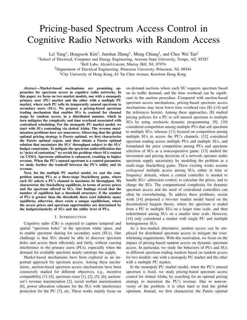
Fig. 1: (a) Monopoly PU Market (b) Multiple PU Market.

region associated with the SUs’ throughput, based on thekey observation that the global optimal strategy is also Paretooptimal. Then, by maximizing the SUs’ throughput subject tothe budget constraints, we provide a Pareto optimal solutionthat takes into account both the spectrum utilization andthe SUs’ budgets. This Pareto optimal solution exhibits adecentralized structure, i.e., the Pareto optimal pricing strategyand access probabilities can be computed by the PU andthe SUs locally. We then develop a distributed pricing-basedspectrum access control algorithm accordingly. To mitigate thespectrum underutilization due to “price of contention,” we nextturn to dynamic spectrum access using CSMA. Improvementsin spectrum utilization and revenue to PU are quantified. Wealso consider the PU’s unused spectrum as a control parameter,when the PU can flexibly allocate the spectrum to its ongoingtransmissions. This enables us to tune the tradeoff between thePU’s utility and its revenue.

In the multiple PU market model, we treat the competitionamong PUs as a three-stage Stackelberg game, where each PUseeks to maximize its net utility. We explore optimal strategiesto adapt the prices and offered spectrum for each PU. Weshow that the equilibria of the game exist and depend on thesystem parameters such as the number of PUs, SUs’ budgetsand demand elasticity. Our results reveal that the number ofequilibria exhibits a threshold phenomenon: if the number ofPUs is greater than the threshold, there exist infinitely manyequilibria, where the equilibrium price reduces to the minimumprice that may cut down PUs’ profit; otherwise, there exists aunique equilibrium. We further provide an iterative algorithmto find the equilibrium.

The rest of the paper is organized as follows. In SectionII, we study the monopoly PU market, and present the Paretooptimal pricing strategy for the PU’s revenue maximizationproblem. We also characterize the tradeoff between the PU’sutility and its revenue. We study the competition among PUsin the multiple PU market in Section III, where we cast thecompetition among PUs as a three-stage Stackelberg game,and analyze the equilibria of the game. Finally, we concludethe paper in Section IV.

II. MONOPOLY PU MARKET

A. System Model

We first consider a monopoly PU market with a set ofSUs, denoted by ℳ. The PU sells the available spectrum

opportunity 𝑐 in each period1, in terms of time slots in a slottedwireless system, to SUs who are willing to buy the spectrumopportunities (Figure 1(a)). In this case, the PU broadcasts theavailability of spectrum opportunities and the prices to accessthe spectrum to the SUs. If a SU decides to buy the spectrumopportunity, it sends a request message to the PU.

We study two cases: 1) the spectrum opportunity 𝑐 is fixed,where the PU desires to find the optimal pricing strategy (theoptimal usage price and flat price) to maximize its revenue; 2)the spectrum opportunity 𝑐 is a control parameter that the PUcan use to balance its own utility and revenue. In both cases,each SU seeks to set its demand that maximizes its payoff,given the spectrum opportunity 𝑐, the usage price 𝑝𝑖, and theflat price 𝑔𝑖.

B. The Case with Fixed Spectrum Opportunity

We first study the case where the spectrum opportunity 𝑐is fixed. We will show that the Pareto optimal usage priceis the same for all SUs, and is uniquely determined by thedemand of each SU and 𝑐. We begin with the channel accessmodel for SUs, assuming a linear pricing strategy, i.e., the PUcharges each SU a flat price and a usage price proportionalto its successful transmissions.

1) Slotted Aloha Model for SUs’ Channel AccessEach SU first carries out spectrum sensing to detect the

PU’s activity. When the sensing result reveals that the PU isidle, SUs will contend for channel access by random access.As in the standard slotted Aloha model, we assume thatall SUs are within the contention ranges of the others andall transmissions are synchronized in each slot. We assumethat SUs always have enough packets to transmit and trafficdemands of SUs are elastic. Denote by 𝑧𝑖 the transmissionprobability of the 𝑖th SU. The probability that the 𝑖th SU’spacket is successfully received is 𝑠𝑖 = 𝑧𝑖

∏𝑗 ∕=𝑖(1 − 𝑧𝑗). The

expected number of successfully transmitted packets of the 𝑖thSU in one period can be written as 𝑠𝑖 = 𝑐𝑠𝑖, where 𝑠𝑖 ∈ [0, 𝑐].Accordingly, the 𝑖th SU receives a utility in one period equalto 𝑈𝑖(𝑠𝑖), where 𝑈𝑖(.) denotes the utility function of the 𝑖thSU. The optimal demand 𝑠∗𝑖 is the solution to the followingoptimization problem:

maximize 𝑈𝑖(𝑠𝑖)− (𝑝𝑖𝑠𝑖 + 𝑔𝑖)subject to 0 ≤ 𝑠𝑖 ≤ 𝑐variable {𝑠𝑖}.

(1)

As is standard, we define the demand function that capturesthe successful transmissions 𝑠𝑖 given the price 𝑝𝑖 as

𝑑𝑖(𝑝𝑖) =

{𝑈 ′−1𝑖 (𝑝𝑖) if 𝑔𝑖 ≤ 𝑈𝑖(𝑠𝑖)− 𝑝𝑖𝑠𝑖,0 otherwise.

(2)

Assuming 𝛼-fair utility functions, the utility and the demand

1The period refers to a time frame that the PU sells its unused part, denotedby 𝑐.

3

functions of each SU can be written, respectively, as:

𝑈𝑖 (𝑠𝑖) =

{𝜎𝑖

1−𝛼 (𝑠𝑖)1−𝛼

0 ≤ 𝛼 < 1,

𝜎𝑖 log (𝑠𝑖) 𝛼 = 1,(3)

𝑑𝑖(𝑝𝑖) =

{𝜎

1𝛼𝑖 𝑝

− 1𝛼

𝑖 if 𝑔𝑖 ≤ 𝑈𝑖(𝑠𝑖)− 𝑝𝑖𝑠𝑖,0 otherwise,

(4)

where 𝜎𝑖, the multiplicative constant in the 𝛼-fair utilityfunction, denotes the utility level2 of the 𝑖th SU, which reflectsthe budget of the 𝑖th SU. Note that we mainly consider thecase of 0 < 𝛼 < 1 because 1

𝛼 = −𝑝𝑖𝑑′𝑖(𝑝𝑖)

𝑑𝑖(𝑝𝑖)is the elasticity of

the demand seen by the PU, and it has to be larger than 1 sothat the monopoly price is finite [17]. Clearly, the 𝛼-fairnessboils down to the weighted proportional fairness when 𝛼 = 1,and to selecting the SU with the highest budget when 𝛼 = 0.

2) PU’s Pricing StrategyWe consider the following revenue maximization problem

for the monopoly PU market:

maximize∑

𝑖∈ℳ (𝑔𝑖 + 𝑝𝑖𝑠𝑖)subject to 𝑠𝑖 ≤ 𝑐𝑧𝑖

∏𝑘 ∕=𝑖(1− 𝑧𝑘), ∀𝑖 ∈ ℳ

𝑠𝑖 = 𝑑𝑖(𝑝𝑖), ∀𝑖 ∈ ℳ𝑈𝑖(𝑠𝑖)− 𝑔𝑖 − 𝑝𝑖𝑠𝑖 ≥ 0, ∀𝑖 ∈ ℳ

variables {g,p, s, z}.

(5)

The constraint 𝑈𝑖(𝑠𝑖) − 𝑔𝑖 − 𝑝𝑖𝑠𝑖 ≥ 0 ensures that SUs havenon-negative utility under the prices 𝑔𝑖 and 𝑝𝑖, without whichSUs choose not to transmit. Let 𝑔∗𝑖 , 𝑝∗𝑖 , 𝑠∗𝑖 and 𝑧∗𝑖 be theoptimal solution to (5). At optimality, we have 𝑈𝑖(𝑠

∗𝑖 )− 𝑔∗𝑖 −

𝑝∗𝑖 𝑠∗𝑖 = 0, ∀𝑖 ∈ ℳ; otherwise, the PU can always increase its

revenue by increasing 𝑔∗𝑖 to make the SU’s net utility zero.Lemma 2.1: The optimal prices for (5) are given by

𝑔𝑖 = 𝑈𝑖(𝑠𝑖)− 𝑝𝑖𝑠𝑖, ∀𝑖 ∈ ℳ. (6)

Based on Lemma 2.1, (5) can be rewritten as:

maximize∑

𝑖∈ℳ 𝑈𝑖(𝑑𝑖(𝑝𝑖))subject to 𝑑𝑖(𝑝𝑖) ≤ 𝑐𝑧𝑖

∏𝑘 ∕=𝑖(1− 𝑧𝑘), ∀𝑖 ∈ ℳ

variables {p, z}.(7)

Since the utility function 𝑈𝑖(⋅) is increasing, the optimal solu-tion to (7) is achieved at the point when 𝑑𝑖(𝑝𝑖) = 𝑐𝑧𝑖

∏𝑘 ∕=𝑖(1−

𝑧𝑘), ∀𝑖 ∈ ℳ. Also, the objective function of (7) can bewritten as 𝑈𝑖(𝑑𝑖(𝑝𝑖)) =

11−𝛼𝑝𝑖𝑑𝑖(𝑝𝑖). Since 1

1−𝛼 is a constant,maximizing 1

1−𝛼

∑𝑖∈ℳ 𝑝𝑖𝑑𝑖(𝑝𝑖) is equivalent to maximizing∑

𝑖∈ℳ 𝑝𝑖𝑑𝑖(𝑝𝑖), i.e., solving (5) is equivalent to solving therevenue maximization problem without considering flat prices:

maximize∑

𝑖∈ℳ 𝑝𝑖𝑑𝑖(𝑝𝑖)subject to 𝑑𝑖(𝑝𝑖) = 𝑐𝑧𝑖

∏𝑘 ∕=𝑖(1− 𝑧𝑘), ∀𝑖 ∈ ℳ

variables {p, z}.(8)

In general, (8) is nonconvex, and therefore it is difficult tofind the global optimum. Since the global optimum of (8) is

2The PU collects the budget information of SUs in each period, whichallows the PU to infer 𝜎𝑖.

0

c

! "i ii Md p c

#$%

c

! "2 2d p

! "1 1d p

c

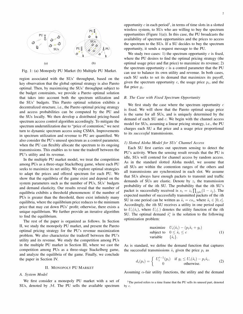
Fig. 2: A sketch of the Pareto optimal region: the case withtwo SUs.

Pareto optimal, we first characterize the Pareto optimal regionof (8). By definition, a feasible allocation s is Pareto optimalif there is no other feasible allocation s′ such that 𝑠′𝑖 ≥ 𝑠𝑖 forall 𝑖 ∈ ℳ and 𝑠′𝑖 > 𝑠𝑖 for some 𝑖.

Lemma 2.2: The Pareto optimal region corresponding to (8)has the following properties:

1) The global optimum is in the Pareto optimal region.2) The solution to (8) is Pareto optimal if and only if∑

𝑖∈ℳ 𝑧𝑖 = 1.Proof: See Appendix A.

By Lemma 2.2, for any Pareto optimal allocation𝑑𝑖(𝑝𝑖), ∀𝑖 ∈ ℳ, we must have

∑𝑖∈ℳ 𝑧𝑖 = 1. Let

𝒜 = {z∣∑𝑖∈ℳ 𝑧𝑖 = 1, 𝑧𝑖 ≥ 0, ∀𝑖 ∈ ℳ} be the Paretooptimal region. Therefore, (8) boils down to searching forthe points in 𝒜 which can maximize (8). In light of Lemma2.2, instead of tackling the original problem given by (8),hereafter we focus on obtaining a Pareto optimal solution to(8) that maximizes SUs’ throughput subject to the SUs’ budgetconstraints, by confining our search space to the hyperplane∑

𝑖∈ℳ 𝑑𝑖(𝑝𝑖) = 𝑐𝜅, where 𝜅 ∈ [0, 1] denotes the spectrumutilization percentage under the allocation 𝑑𝑖(𝑝𝑖), ∀𝑖 ∈ ℳ.

In what follows, we consider this “constrained” version of(8), which simplifies the original problem substantially, tofinding the maximum feasible spectrum utilization 𝜅∗, i.e., thetangent point of the hyperplane and 𝒜, as illustrated in Figure2:

maximize∑

𝑖∈ℳ 𝑝𝑖𝑑𝑖(𝑝𝑖)subject to

∑𝑖∈ℳ 𝑑𝑖(𝑝𝑖) = 𝑐𝜅

𝑑𝑖(𝑝𝑖) = 𝑐𝑧𝑖∏

𝑘 ∕=𝑖(1− 𝑧𝑘), ∀𝑖 ∈ ℳvariables {p, z, 𝜅}.

(9)

We note that the solution to (9) is in general suboptimalto (8). However, by exploring the connections between thepricing strategy and the spectrum utilization, we are able toderive a closed form solution to (9) that is also a Pareto optimalsolution to (8).

Proposition 2.1: For 𝛼 ∈ (0, 1), the optimal solution to (9)is given by

𝑝∗𝑖 =(

𝐺𝑐𝜅∗

)𝛼, ∀𝑖 ∈ ℳ,

𝑔∗𝑖 = 𝑈𝑖(𝑑𝑖(𝑝∗𝑖 ))− 𝑝∗𝑖 𝑑𝑖(𝑝

∗𝑖 ), ∀𝑖 ∈ ℳ,

𝜅∗ =∑

𝑖∈ℳ 𝑧∗𝑖∏

𝑗 ∕=𝑖(1− 𝑧∗𝑗 ),𝑧∗𝑖 = 𝑤𝑖

𝑤𝑖+𝑒−𝑢 , ∀𝑖 ∈ ℳ,

(10)

4

where 𝑤𝑖 = 𝜎1𝛼𝑖 𝐺−1, 𝐺 =

∑𝑖∈ℳ 𝜎

1𝛼𝑖 , and 𝑢 is the unique

solution of ∑𝑖∈ℳ

𝑤𝑖

𝑤𝑖 + 𝑒−𝑢= 1.

Proof: See Appendix B.Next, we sketch a proof outline for the above proposition.

First, the following result establishes the relationship betweenthe optimal pricing strategy of (9) and 𝜅 when 𝛼 ∈ (0, 1).

Lemma 2.3: Given 𝜅, the optimal pricing strategy of (9) for𝛼 ∈ (0, 1) is given by

𝑝∗𝑖 =

(𝐺

𝑐𝜅

)𝛼

, ∀𝑖 ∈ ℳ. (11)

Proof: See Appendix C.A next key step is to find 𝜅∗. By Lemma 2.3, we have

𝑑𝑖(𝑝∗𝑖 ) = 𝜎

1𝛼𝑖 𝐺−1𝑐𝜅, ∀𝑖 ∈ ℳ. Utilizing those constraints, we

can find 𝜅∗ by solving the following problem:

maximize 𝜅subject to 𝑤𝑖𝜅 ≤ 𝑧𝑖

∏𝑗 ∕=𝑖(1− 𝑧𝑗), ∀𝑖 ∈ ℳ

variables {𝜅, z},(12)

where 𝑤𝑖 = 𝜎1𝛼𝑖 𝐺−1. Still, (40) is nonconvex, but by first

taking logarithms of both the objective function and theconstraints and then letting 𝜅′ = log(𝜅), we can transform(40) into the following convex problem:

maximize 𝜅′

subject to ∀𝑖 ∈ ℳlog(𝑤𝑖) + 𝜅′ ≤ log(𝑧𝑖) +

∑𝑗 ∕=𝑖 log(1− 𝑧𝑗),

variables {𝜅′, z}.(13)

Thus, the optimal solution to (40) can be summarized by thefollowing lemma.

Lemma 2.4: The optimal solution to (40) is given by

𝜅∗ =∑

𝑖∈ℳ 𝑧∗𝑖∏

𝑗 ∕=𝑖(1− 𝑧∗𝑗 ),𝑧∗𝑖 = 𝑤𝑖

𝑤𝑖+𝑒−𝑢 , ∀𝑖 ∈ ℳ,(14)

where 𝑢 is the unique solution of∑𝑖∈ℳ

𝑤𝑖

𝑤𝑖 + 𝑒−𝑢= 1. (15)

Further, when the number of SUs in the network is large, i.e.,∣ℳ∣ → ∞, we can approximate 𝜅∗ by 𝑒−1.

Proof: See Appendix D.Based on Lemma 2.3 and Lemma 2.4, the optimal solution

to (9) is given by Proposition 2.1, which is a Pareto optimalsolution to (5).

So far we have focused on the case with 𝛼 ∈ (0, 1). Nowwe consider the corner cases when 𝛼 = 0 and 1. Interestingly,we will see that the Pareto optimal solutions are also globaloptimal in those corner cases.

Corollary 2.1: When 𝛼 = 0, the Pareto optimal solution to(5) is also the global optimal solution, which is given by

𝑝∗𝑖 = max𝑖∈ℳ 𝜎𝑖,

𝑧∗𝑖 =

{1, 𝑖 = 𝑘

0, 𝑖 ∕= 𝑘,

𝑔∗𝑖 = 0,

(16)

for all 𝑖, where 𝑘 = argmax𝑗∈ℳ 𝜎𝑗 .Corollary 2.1 implies that, when 𝛼 = 0, the PU selects the

SU with the highest budget and only allows that SU to accessthe channel with probability 1 to maximize its revenue.

Remarks: The Pareto optimal solution in (10) converges tothe globally optimal solution as 𝛼 goes to zero, i.e.,

𝑝∗𝑖 =

(𝐺

𝑐𝜅∗

)𝛼

=

(1

𝑐𝜅∗

)𝛼⎛⎝∑

𝑗∈ℳ𝜎

1𝛼𝑗

⎞⎠𝛼

→ max𝑗∈ℳ

𝜎𝑗 . (17)

When 𝛼 = 1, (7) can be transformed into a convex problemby taking logarithms of the constraints, and the global optimalaccess probabilities of SUs in this case are

𝑧∗𝑖 =𝜎𝑖∑

𝑘∈ℳ 𝜎𝑘, ∀𝑖 ∈ ℳ,

i.e., the random access probability is proportional to SU’sutility level, where the revenue is dominated by the flat rate,which shares the same spirit of the results in [15]. As 𝛼 goesto 1, the revenue computed by (10) also converges to theglobal optimal solution, since the Pareto optimal flat rates in(10) converge to the global optimal ones, which dominate therevenue.

3) Distributed Implementation of Spectrum Access ControlBased on the above study, next, we develop a distributed

implementation of the pricing-based spectrum access control.Based on Proposition 2.1, the Pareto optimal solution exhibitsa decentralized structure, which we now exploit to develop adistributed pricing-based spectrum access control as follows.

Algorithm 1 Distributed Pricing-based Spectrum Access Con-trol

1) The PU collects the budget information of SUs, i.e., {𝜎𝑖}.2) The PU computes 𝑝∗, g∗, 𝐺 and 𝑢 by (10), and broadcasts𝑝∗, 𝐺 and 𝑢 to SUs.3) Each SU computes 𝑧∗𝑖 by (10) based on 𝐺 and 𝑢, andinfers g∗ from its own utility and 𝑝∗ by (10).At the beginning of each periodIf New SUs join the system then

The new SUs inform the PU of their {𝜎𝑖}. Then run Steps2 to 3.EndifIf SUs leave the system then

The leaving SUs inform the PU. Then run Steps 2 to 3.Endif

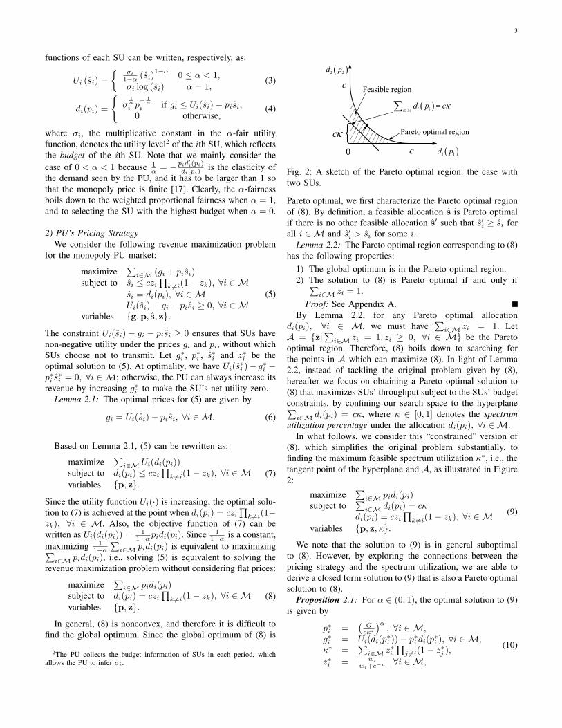
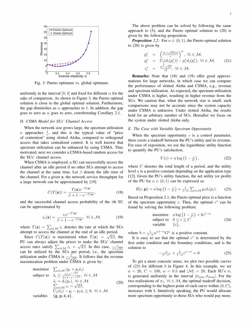
C. Numerical Example: Pareto Optimum vs. Global Optimum

To reduce the computational complexity in solving theglobal optimum of (5), under slotted Aloha, we first solve(9). To examine the efficiency of this Pareto optimal solution,we exhaustively search for the global optimum of (5) tocompare with the Pareto optimum, in a small network withthree SUs so as to efficiently generate the true global optimumas the benchmark. Here 𝑐 is 5, and each SU’s 𝜎𝑖 is generated

5

0 0.2 0.4 0.6 0.8 10

5

10

15

20

25

30

35

40

Inverse elasticity: α

Rev

enue

Pareto OptimumGlobal Optimum

Fig. 3: Pareto optimum vs. global optimum.

uniformly in the interval [0, 4] and fixed for different 𝛼 for thesake of comparison. As shown in Figure 3, the Pareto optimalsolution is close to the global optimal solution. Furthermore,the gap diminishes as 𝛼 approaches to 1. In addition, the gapgoes to zero as 𝛼 goes to zero, corroborating Corollary 2.1.

D. CSMA Model for SUs’ Channel Access

When the network size grows large, the spectrum utilization𝜅 approaches 1

𝑒 , and this is the typical value of “priceof contention” using slotted Aloha, compared to orthogonalaccess that takes centralized control. It is well known thatspectrum utilization can be enhanced by using CSMA. Thusmotivated, next we consider a CSMA-based random access forthe SUs’ channel access.

When CSMA is employed, a SU can successfully access thechannel after an idle period if no other SUs attempt to accessthe channel at the same time. Let 𝛽 denote the idle time ofthe channel. For a given z, the network service throughput fora large network can be approximated by [19]

𝐶(𝑇 (z)) =𝑇 (z)𝑒−𝑇 (z)

𝛽 + 1− 𝑒−𝑇 (z), (18)

and the successful channel access probability of the 𝑖th SUcan be approximated by

𝑠𝑖(z) =𝑧𝑖𝑒

−𝑇 (z)

𝛽 + 1− 𝑒−𝑇 (z), ∀𝑖 ∈ ℳ, (19)

where 𝑇 (z) =∑

𝑖∈ℳ 𝑧𝑖 denotes the rate at which the SUsattempt to access the channel at the end of an idle period.

Since 𝐶(𝑇 (z)) is maximized when 𝑇 (z) =√2𝛽, the

PU can always adjust the prices to make the SUs’ channelaccess rates satisfy

∑𝑖∈ℳ 𝑧𝑖 =

√2𝛽. In this case, 𝑐

1+√2𝛽

can be utilized by the SUs per period, i.e., the spectrumutilization under CSMA is 1

1+√2𝛽

. It follows that the revenuemaximization problem under CSMA is given by:

maximize∑

𝑖∈ℳ (𝑔𝑖 + 𝑝𝑖𝑠𝑖)

subject to 𝑠𝑖 ≤ 𝑐𝑧𝑖𝑒−√

2𝛽

𝛽+1−𝑒−√

2𝛽 , ∀𝑖 ∈ ℳ𝑠𝑖 = 𝑑𝑖(𝑝𝑖), ∀𝑖 ∈ ℳ∑

𝑖∈ℳ 𝑧𝑖 =√2𝛽,

𝑈𝑖(𝑠𝑖)− 𝑔𝑖 − 𝑝𝑖𝑠𝑖 ≥ 0, ∀𝑖 ∈ ℳvariables {g,p, s, z}.

(20)

The above problem can be solved by following the sameapproach to (5), and the Pareto optimal solution to (20) isgiven by the following proposition.

Proposition 2.2: For 𝛼 ∈ (0, 1), the Pareto optimal solutionto (20) is given by

𝑝∗𝑖 =(

(1+√2𝛽)𝐺𝑐

)𝛼

, ∀𝑖 ∈ ℳ,

𝑔∗𝑖 = 𝑈𝑖(𝑑𝑖(𝑝∗𝑖 ))− 𝑝∗𝑖 𝑑𝑖(𝑝

∗𝑖 ), ∀𝑖 ∈ ℳ,

𝑧∗𝑖 =𝜎

1𝛼𝑖

√2𝛽

𝐺 , ∀𝑖 ∈ ℳ.

(21)

Remarks: Note that (18) and (19) offer good approxi-mations for large networks, in which case we can comparethe performance of slotted Aloha and CSMA, e.g., revenueand spectrum utilization. As expected, the spectrum utilizationunder CSMA is higher, resulting in higher revenue from theSUs. We caution that, when the network size is small, suchcomparisons may not be accurate since the system capacityunder CSMA is unknown. Under slotted Aloha, the resultshold for an arbitrary number of SUs. Hereafter we focus onthe system under slotted Aloha only.

E. The Case with Variable Spectrum Opportunity

When the spectrum opportunity 𝑐 is a control parameter,there exists a tradeoff between the PU’s utility and its revenue.For ease of exposition, we use the logarithmic utility functionto quantify the PU’s satisfaction,

𝑉 (𝑐) = 𝑎 log(1− 𝑐

𝐶

), (22)

where 𝐶 denotes the total length of a period, and the utilitylevel 𝑎 is a positive constant depending on the application type[12]. Given the PU’s utility function, the net utility (or profit)of the PU for 𝛼 ∈ (0, 1) can be expressed as:

𝑅(𝑐,p) = 𝑎 log(1− 𝑐

𝐶

)+ 1

1−𝛼

∑𝑖∈ℳ 𝑝𝑖𝑑𝑖(𝑝𝑖). (23)

Based on Proposition 2.1, the Pareto optimal price is a functionof the spectrum opportunity 𝑐. Then, the optimal 𝑐∗ can befound by solving the following problem:

maximize 𝑎 log(1− 𝑐

𝐶

)+ 𝑏𝑐1−𝛼

subject to 0 ≤ 𝑐 ≤ 𝐶variable {𝑐},

(24)

where 𝑏 = 11−𝛼𝜅

∗1−𝛼𝐺𝛼 is a positive constant.It is easy to see that the optimal 𝑐∗ is determined by the

first order condition and the boundary conditions, and is thesolution to

− 𝑎𝐶−𝑐∗ + 𝑏

1−𝛼𝑐∗−𝛼 = 0. (25)

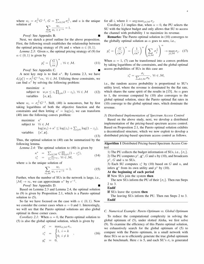
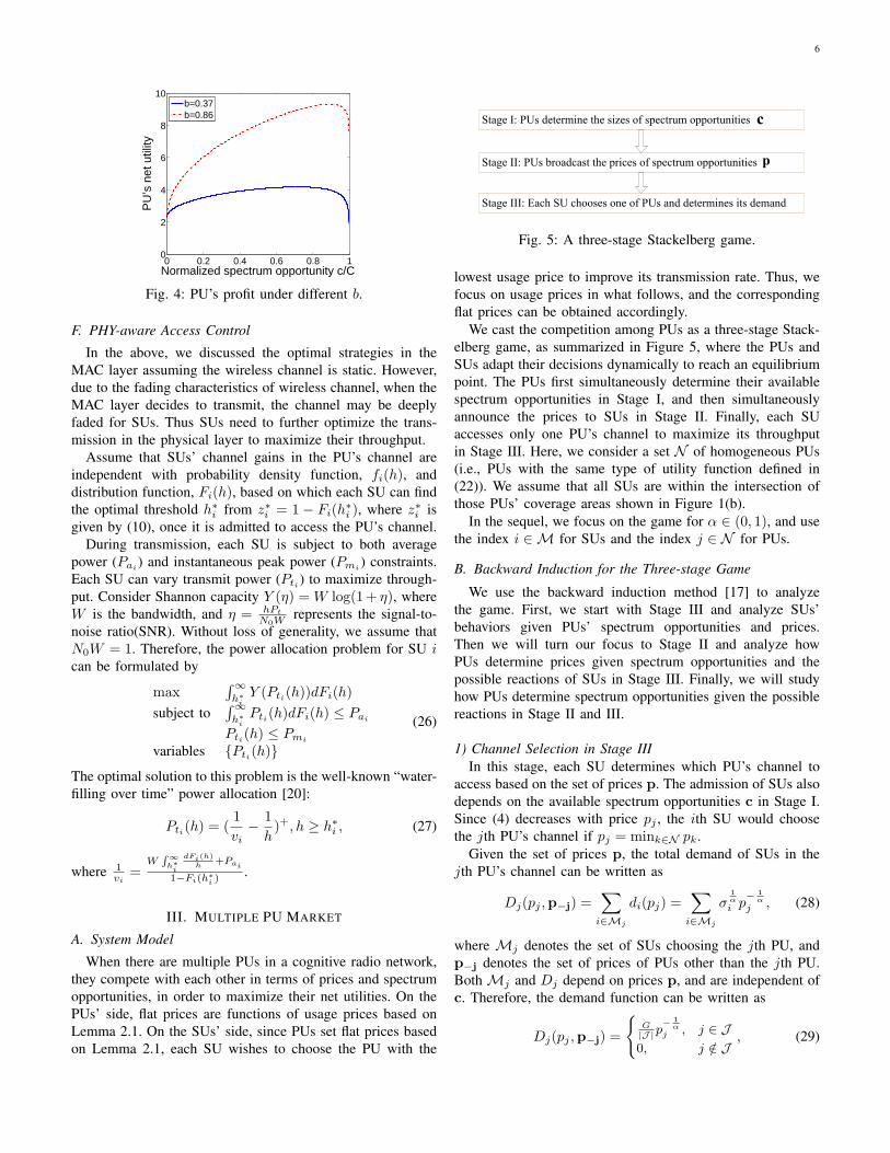
To get a more concrete sense, we plot two possible curvesof (23) for different 𝑏 in Figure 4. In this example, we set𝑎 = 20, 𝐶 = 100, 𝛼 = 0.5 and ∣ℳ∣ = 20. Each SU’s 𝜎𝑖

is generated uniformly in the interval [𝜎min, 𝜎max]. For thetwo realizations of 𝜎𝑖, ∀𝑖 ∈ ℳ, the optimal tradeoff decision,corresponding to the highest point of each curve within (0, 𝐶),increases with 𝑏. Intuitively speaking, the PU would allocatemore spectrum opportunity to those SUs who would pay more.

6

0 0.2 0.4 0.6 0.8 10

2

4

6

8

10

Normalized spectrum opportunity c/C

PU

’s n

et u

tility

b=0.37b=0.86

Fig. 4: PU’s profit under different 𝑏.

F. PHY-aware Access Control

In the above, we discussed the optimal strategies in theMAC layer assuming the wireless channel is static. However,due to the fading characteristics of wireless channel, when theMAC layer decides to transmit, the channel may be deeplyfaded for SUs. Thus SUs need to further optimize the trans-mission in the physical layer to maximize their throughput.

Assume that SUs’ channel gains in the PU’s channel areindependent with probability density function, 𝑓𝑖(ℎ), anddistribution function, 𝐹𝑖(ℎ), based on which each SU can findthe optimal threshold ℎ∗

𝑖 from 𝑧∗𝑖 = 1 − 𝐹𝑖(ℎ∗𝑖 ), where 𝑧∗𝑖 is

given by (10), once it is admitted to access the PU’s channel.During transmission, each SU is subject to both average

power (𝑃𝑎𝑖) and instantaneous peak power (𝑃𝑚𝑖 ) constraints.Each SU can vary transmit power (𝑃𝑡𝑖) to maximize through-put. Consider Shannon capacity 𝑌 (𝜂) = 𝑊 log(1+ 𝜂), where𝑊 is the bandwidth, and 𝜂 = ℎ𝑃𝑡

𝑁0𝑊represents the signal-to-

noise ratio(SNR). Without loss of generality, we assume that𝑁0𝑊 = 1. Therefore, the power allocation problem for SU 𝑖can be formulated by

max∫∞ℎ∗𝑖𝑌 (𝑃𝑡𝑖(ℎ))𝑑𝐹𝑖(ℎ)

subject to∫∞ℎ∗𝑖𝑃𝑡𝑖(ℎ)𝑑𝐹𝑖(ℎ) ≤ 𝑃𝑎𝑖

𝑃𝑡𝑖(ℎ) ≤ 𝑃𝑚𝑖

variables {𝑃𝑡𝑖(ℎ)}(26)

The optimal solution to this problem is the well-known “water-filling over time” power allocation [20]:

𝑃𝑡𝑖(ℎ) = (1

𝑣𝑖− 1

ℎ)+, ℎ ≥ ℎ∗

𝑖 , (27)

where 1𝑣𝑖

=𝑊

∫ ∞ℎ∗𝑖

𝑑𝐹𝑖(ℎ)

ℎ +𝑃𝑎𝑖

1−𝐹𝑖(ℎ∗𝑖 )

.

III. MULTIPLE PU MARKET

A. System Model

When there are multiple PUs in a cognitive radio network,they compete with each other in terms of prices and spectrumopportunities, in order to maximize their net utilities. On thePUs’ side, flat prices are functions of usage prices based onLemma 2.1. On the SUs’ side, since PUs set flat prices basedon Lemma 2.1, each SU wishes to choose the PU with the

Stage I: PUs determine the sizes of spectrum opportunities

Stage II: PUs broadcast the prices of spectrum opportunities p

Stage III: Each SU chooses one of PUs and determines its demand

c

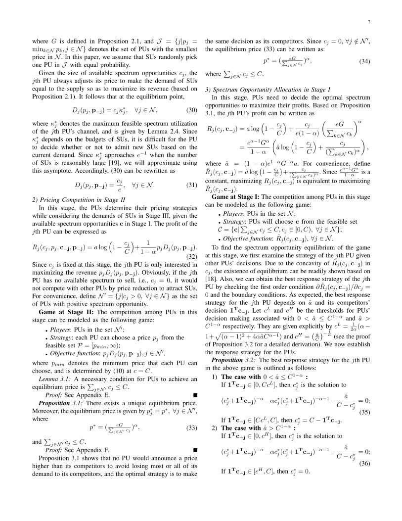
Fig. 5: A three-stage Stackelberg game.

lowest usage price to improve its transmission rate. Thus, wefocus on usage prices in what follows, and the correspondingflat prices can be obtained accordingly.

We cast the competition among PUs as a three-stage Stack-elberg game, as summarized in Figure 5, where the PUs andSUs adapt their decisions dynamically to reach an equilibriumpoint. The PUs first simultaneously determine their availablespectrum opportunities in Stage I, and then simultaneouslyannounce the prices to SUs in Stage II. Finally, each SUaccesses only one PU’s channel to maximize its throughputin Stage III. Here, we consider a set 𝒩 of homogeneous PUs(i.e., PUs with the same type of utility function defined in(22)). We assume that all SUs are within the intersection ofthose PUs’ coverage areas shown in Figure 1(b).

In the sequel, we focus on the game for 𝛼 ∈ (0, 1), and usethe index 𝑖 ∈ ℳ for SUs and the index 𝑗 ∈ 𝒩 for PUs.

B. Backward Induction for the Three-stage Game

We use the backward induction method [17] to analyzethe game. First, we start with Stage III and analyze SUs’behaviors given PUs’ spectrum opportunities and prices.Then we will turn our focus to Stage II and analyze howPUs determine prices given spectrum opportunities and thepossible reactions of SUs in Stage III. Finally, we will studyhow PUs determine spectrum opportunities given the possiblereactions in Stage II and III.

1) Channel Selection in Stage IIIIn this stage, each SU determines which PU’s channel to

access based on the set of prices p. The admission of SUs alsodepends on the available spectrum opportunities c in Stage I.Since (4) decreases with price 𝑝𝑗 , the 𝑖th SU would choosethe 𝑗th PU’s channel if 𝑝𝑗 = min𝑘∈𝒩 𝑝𝑘.

Given the set of prices p, the total demand of SUs in the𝑗th PU’s channel can be written as

𝐷𝑗(𝑝𝑗 ,p−j) =∑𝑖∈ℳ𝑗

𝑑𝑖(𝑝𝑗) =∑𝑖∈ℳ𝑗

𝜎1𝛼𝑖 𝑝

− 1𝛼

𝑗 , (28)

where ℳ𝑗 denotes the set of SUs choosing the 𝑗th PU, andp−j denotes the set of prices of PUs other than the 𝑗th PU.Both ℳ𝑗 and 𝐷𝑗 depend on prices p, and are independent ofc. Therefore, the demand function can be written as

𝐷𝑗(𝑝𝑗 ,p−j) =

{𝐺∣𝒥 ∣𝑝

− 1𝛼

𝑗 , 𝑗 ∈ 𝒥0, 𝑗 /∈ 𝒥 , (29)

7

where 𝐺 is defined in Proposition 2.1, and 𝒥 = {𝑗∣𝑝𝑗 =min𝑘∈𝒩 𝑝𝑘, 𝑗 ∈ 𝒩} denotes the set of PUs with the smallestprice in 𝒩 . In this paper, we assume that SUs randomly pickone PU in 𝒥 with equal probability.

Given the size of available spectrum opportunities 𝑐𝑗 , the𝑗th PU always adjusts its price to make the demand of SUsequal to the supply so as to maximize its revenue (based onProposition 2.1). It follows that at the equilibrium point,

𝐷𝑗(𝑝𝑗 ,p−j) = 𝑐𝑗𝜅∗𝑗 , ∀𝑗 ∈ 𝒩 , (30)

where 𝜅∗𝑗 denotes the maximum feasible spectrum utilization

of the 𝑗th PU’s channel, and is given by Lemma 2.4. Since𝜅∗𝑗 depends on the budgets of SUs, it is difficult for the PU

to decide whether or not to admit new SUs based on thecurrent demand. Since 𝜅∗

𝑗 approaches 𝑒−1 when the numberof SUs is reasonably large [19], we will approximate usingthis asymptote. Accordingly, (30) can be rewritten as

𝐷𝑗(𝑝𝑗 ,p−j) =𝑐𝑗𝑒, ∀𝑗 ∈ 𝒩 . (31)

2) Pricing Competition in Stage IIIn this stage, the PUs determine their pricing strategies

while considering the demands of SUs in Stage III, given theavailable spectrum opportunities c in Stage I. The profit of the𝑗th PU can be expressed as

𝑅𝑗(𝑐𝑗 , 𝑝𝑗 , c−j,p−j) = 𝑎 log(1− 𝑐𝑗

𝐶

)+

1

1− 𝛼𝑝𝑗𝐷𝑗(𝑝𝑗 ,p−j).

(32)Since 𝑐𝑗 is fixed at this stage, the 𝑗th PU is only interested inmaximizing the revenue 𝑝𝑗𝐷𝑗(𝑝𝑗 ,p−j). Obviously, if the 𝑗thPU has no available spectrum to sell, i.e., 𝑐𝑗 = 0, it wouldnot compete with other PUs by price reduction to attract SUs.For convenience, define 𝒩 ′ = {𝑗∣𝑐𝑗 > 0, ∀𝑗 ∈ 𝒩} as the setof PUs with positive spectrum opportunity.

Game at Stage II: The competition among PUs in thisstage can be modeled as the following game:

∙ Players: PUs in the set 𝒩 ′;∙ Strategy: each PU can choose a price 𝑝𝑗 from thefeasible set 𝒫 = [𝑝𝑚𝑖𝑛,∞);∙ Objective function: 𝑝𝑗𝐷𝑗(𝑝𝑗 ,p−j), 𝑗 ∈ 𝒩 ′,

where 𝑝𝑚𝑖𝑛 denotes the minimum price that each PU canchoose, and is determined by (10) at 𝑐 = 𝐶.

Lemma 3.1: A necessary condition for PUs to achieve anequilibrium price is

∑𝑗∈𝒩 ′ 𝑐𝑗 ≤ 𝐶.

Proof: See Appendix E.Proposition 3.1: There exists a unique equilibrium price.

Moreover, the equilibrium price is given by 𝑝∗𝑗 = 𝑝∗, ∀𝑗 ∈ 𝒩 ′,where

𝑝∗ = ( 𝑒𝐺∑𝑗∈𝒩′ 𝑐𝑗

)𝛼, (33)

and∑

𝑗∈𝒩 ′ 𝑐𝑗 ≤ 𝐶.Proof: See Appendix F.

Proposition 3.1 shows that no PU would announce a pricehigher than its competitors to avoid losing most or all of itsdemand to its competitors, and the optimal strategy is to make

the same decision as its competitors. Since 𝑐𝑗 = 0, ∀𝑗 /∈ 𝒩 ′,the equilibrium price (33) can be written as:

𝑝∗ = ( 𝑒𝐺∑𝑗∈𝒩 𝑐𝑗

)𝛼, (34)

where∑

𝑗∈𝒩 𝑐𝑗 ≤ 𝐶.

3) Spectrum Opportunity Allocation in Stage IIn this stage, PUs need to decide the optimal spectrum

opportunities to maximize their profits. Based on Proposition3.1, the jth PU’s profit can be written as

𝑅𝑗(𝑐𝑗 , c−j) = 𝑎 log(1− 𝑐𝑗

𝐶

)+

𝑐𝑗𝑒(1− 𝛼)

(𝑒𝐺∑𝑘∈𝒩 𝑐𝑘

)𝛼

=𝑒𝛼−1𝐺𝛼

1− 𝛼

(�� log

(1− 𝑐𝑗

𝐶

)+

𝑐𝑗(∑

𝑘∈𝒩 𝑐𝑘)𝛼

),

where �� = (1 − 𝛼)𝑒1−𝛼𝐺−𝛼𝑎. For convenience, define��𝑗(𝑐𝑗 , c−j) = �� log

(1− 𝑐𝑗

𝐶

)+

𝑐𝑗(∑

𝑘∈𝒩 𝑐𝑘)𝛼. Since 𝑒𝛼−1𝐺𝛼

1−𝛼 is aconstant, maximizing 𝑅𝑗(𝑐𝑗 , c−j) is equivalent to maximizing��𝑗(𝑐𝑗 , c−j).

Game at Stage I: The competition among PUs in this stagecan be modeled as the following game:

∙ Players: PUs in the set 𝒩 ;∙ Strategy: PUs will choose c from the feasible set𝒞 = {c∣∑𝑗∈𝒩 𝑐𝑗 ≤ 𝐶, 𝑐𝑗 ∈ [0, 𝐶), ∀𝑗 ∈ 𝒩};∙ Objective function: ��𝑗(𝑐𝑗 , c−j), ∀𝑗 ∈ 𝒩 .

To find the spectrum opportunity equilibrium of the gameat this stage, we first examine the strategy of the 𝑗th PU givenother PUs’ decisions. Due to the concavity of ��𝑗(𝑐𝑗 , c−j) in𝑐𝑗 , the existence of equilibrium can be readily shown based on[18]. Also, we can obtain the best response strategy of the 𝑗thPU by checking the first order condition ∂��𝑗(𝑐𝑗 , c−j)/∂𝑐𝑗 =0 and the boundary conditions. As expected, the best responsestrategy for the 𝑗th PU depends on �� and its competitors’decision 1Tc−j. Let 𝑐𝐿 and 𝑐𝐻 be the thresholds for PUs’decision making associated with 0 < �� ≤ 𝐶1−𝛼 and �� >𝐶1−𝛼 respectively. They are given explicitly by 𝑐𝐿 = 1

2𝛼 (𝛼−1+

√(𝛼− 1)2 + 4𝛼��𝐶𝛼−1) and 𝑐𝐻 =

(��𝐶

)− 1𝛼 (see the proof

of Proposition 3.2 for a detailed derivation). We now establishthe response strategy for the PUs.

Proposition 3.2: The best response strategy for the 𝑗th PUin the above game is outlined as follows:

1) The case with 0 < �� ≤ 𝐶1−𝛼 :If 1Tc−j ∈ [0, 𝐶𝑐𝐿], then 𝑐∗𝑗 is the solution to

(𝑐∗𝑗 +1Tc−j)−𝛼−𝛼𝑐∗𝑗 (𝑐

∗𝑗 +1Tc−j)

−𝛼−1− ��

𝐶 − 𝑐∗𝑗= 0;

(35)If 1Tc−j ∈ [𝐶𝑐𝐿, 𝐶], then 𝑐∗𝑗 = 𝐶 − 1Tc−j.

2) The case with �� > 𝐶1−𝛼 :If 1Tc−j ∈ [0, 𝑐𝐻 ], then 𝑐∗𝑗 is the solution to

(𝑐∗𝑗 +1Tc−j)−𝛼−𝛼𝑐∗𝑗 (𝑐

∗𝑗 +1Tc−j)

−𝛼−1− ��

𝐶 − 𝑐∗𝑗= 0;

(36)If 1Tc−j ∈ [𝑐𝐻 , 𝐶], then 𝑐∗𝑗 = 0.

8

Proof: See Appendix G.As expected, the equilibrium of Game at Stage I depends

on ��, 𝛼, 𝑐𝐿, and the number of PUs. For convenience,define 𝒩1 = {𝑗∣𝑐∗𝑗 is the solution to (35), ∀𝑗 ∈ 𝒩} and𝒩2 = {𝑗∣𝑐∗𝑗 = 𝐶 − 1Tc−j, ∀𝑗 ∈ 𝒩}. Observe that 𝒩1

represents the set of PUs whose competitors’ decision isbelow the threshold 𝐶𝑐𝐿, while 𝒩2 represents the set of PUswhose competitors’ decision is above the threshold 𝐶𝑐𝐿. Thespectrum opportunity equilibria of Game at Stage I are givenby the following proposition.

Proposition 3.3: The spectrum opportunity equilibria inStage I are summarized as follows:

1) The case with 0 < �� ≤ 𝐶1−𝛼 :a) If 𝑐𝐿 ≤ ∣𝒩 ∣−1

∣𝒩 ∣ (i.e., 𝒩1 ∕= ∅ and 𝒩2 ∕= ∅),there exist infinitely many spectrum opportunityequilibria satisfying∑

𝑗2∈𝒩2

𝑐∗𝑗2 = 𝐶 − ∣𝒩1∣𝐶(1− 𝑐𝐿),

𝑐∗𝑗1 = 𝐶(1− 𝑐𝐿), ∀𝑗1 ∈ 𝒩1,

𝐶 − 𝑐∗𝑗2 ≥ 𝐶𝑐𝐿, ∀𝑗2 ∈ 𝒩2.

b) If 𝑐𝐿 > ∣𝒩 ∣−1∣𝒩 ∣ (i.e., 𝒩1 = 𝒩 and 𝒩2 = ∅), there

exists a unique spectrum opportunity equilibriumsuch that 𝑐∗𝑗 = 𝑐∗, ∀𝑗 ∈ 𝒩 , where 𝑐∗ is the solutionto

(∣𝒩 ∣𝑐∗)−𝛼(1− 𝛼∣𝒩 ∣ ) =

��𝐶−𝑐∗ . (37)

2) The case with �� > 𝐶1−𝛼 :There exists a unique spectrum opportunity equilibriumsuch that 𝑐∗𝑗 = 𝑐∗, ∀𝑗 ∈ 𝒩 , and lies in the strict interior(0, 1

∣𝒩 ∣ (��𝐶 )−

1𝛼 ), where 𝑐∗ is the solution to

(∣𝒩 ∣𝑐∗)−𝛼(1− 𝛼∣𝒩 ∣ ) =

��𝐶−𝑐∗ . (38)

Proof: See Appendix H.Based on Proposition 3.3, we can see that there exists a

threshold for the number of PUs, denoted by 𝑁𝑃𝑈 , in thecase with 0 < �� ≤ 𝐶1−𝛼, where 𝑁𝑃𝑈 is given by 1

1−𝑐𝐿.

Accordingly, Proposition 3.3 can be treated as a criterion forPUs to decide whether to join the competition or not, becauseeach PU can calculate the pricing equilibrium when it gathersthe necessary information based on Proposition 3.3. In the casewith 0 < �� ≤ 𝐶1−𝛼, it needs to check whether the condition𝑁𝑃𝑈 > ∣𝒩 ∣ holds. This is because if 𝑁𝑃𝑈 ≤ ∣𝒩 ∣ after it joinsthe competition, the pricing equilibrium will be 𝑝min, whichmay make it unprofitable to offer its spectrum to SUs.

C. An Algorithm for Computing Equilibria

To achieve the equilibrium of the dynamic game, we presentan iterative algorithm for each PU. Based on Lemma 3.1,if

∑𝑗∈𝒩 𝑐𝑗 > 𝐶, the spectrum allocation is inefficient, i.e.,

there always exists some PU whose supply is larger than thedemand. Thus, each PU first updates its spectrum opportunitybased on the demand to fully utilize its spectrum. Oncethe necessary condition

∑𝑗∈𝒩 𝑐𝑗 ≤ 𝐶 is satisfied, each

PU can update its spectrum opportunity in the Stage I by

Proposition 3.2. We assume that the “total budget” 𝐺 of SUs isavailable to each PU. The proposed algorithm for computingthe market equilibrium is summarized in Algorithm 2. Basedon Lemma 3.1, Proposition 3.2 and Proposition 3.3, Algorithm2 converges to the equilibrium of the game, as also verifiedby simulation.

Algorithm 2 Computing the equilibrium of the multiple PUmarket

Initialization: Each PU collects the budget information ofSUs, i.e., {𝜎𝑖}.At the beginning of each period1) If

∑𝑗∈𝒩 𝑐𝑗 > 𝐶 then

Each PU sets 𝑐𝑗 = 𝐷𝑗(𝑝𝑗 ,p−j), and broadcasts 𝑐𝑗 .Else

Each PU sets 𝑐𝑗 based on Proposition 3.2, and broad-casts 𝑐𝑗 .

Endif2) Each PU sets 𝑝𝑗 = max

(𝑝min,

(𝑒𝐺∑

𝑗∈𝒩 𝑐𝑗

)𝛼), and

broadcasts 𝑝𝑗 .3) Each SU randomly chooses a PU’s channel with thelowest price.4) Each PU admits new SUs when 𝑐𝑗 > 𝐷𝑗(𝑝𝑗 ,p−j).5) Steps 1 to 4 are repeated in each period.

Remarks: Algorithm 2 is applicable to the scenarios, wherethe PUs can vary their spectrum opportunities. When thespectrum opportunities are fixed, the three-stage game reducesto a two-stage game without the stage of spectrum opportunityallocation. In this case, the equilibrium of the game is givenby Proposition 3.1.

D. Numerical Examples: Equilibria of Competitive PUs

Based on Lemma 3.1, there always exists an equilibrium inthe feasible region (i.e.,

∑𝑗∈𝒩 𝑐𝑗 ≤ 𝐶). In the following, we

first illustrate the existence and uniqueness of the equilibriumby (35) for two PUs, in the case with 0 < �� ≤ 𝐶1−𝛼 and𝑐𝐿 > 0.5. Then we consider a more general system modelwith four PUs and examine the convergence of spectrumopportunities. Finally, we demonstrate how the equilibriumprice evolves under different elasticities of SUs and differentnumbers of PUs. In each experiment, 𝐶 is equal to 20, andeach SU’s budget 𝜎𝑖 is generated uniformly in the interval[0, 4], and is fixed for different 𝛼 for the sake of comparison.

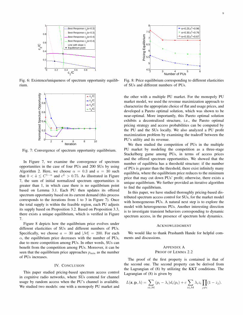
The existence and uniqueness of the equilibrium, corre-sponding to the competitive spectrum opportunity of twoPUs, is illustrated in Figure 6. In particular, we change theinverse elasticity (i.e., 𝛼) of SUs from 0.3 to 0.4 in orderto show how the spectrum opportunity equilibrium evolves,when 0 < �� ≤ 𝐶1−𝛼 and 𝑐𝐿 > 0.5. Based on Proposition3.3, there exists a unique spectrum opportunity equilibrium,which is shown in Figure 6. Furthermore, we observe that thespectrum equilibrium increases with 𝛼, and lies on the linewith slope one, which is due to the symmetry of the bestresponse functions.

9

0 0.2 0.4 0.6 0.8 10

0.2

0.4

0.6

0.8

1

c1/C

c 2/C

Best Response c2(α=0.3)

Best Response c1(α=0.3)

Best Response c2(α=0.4)

Best Response c1(α=0.4)

Line with slope 1Equilibrium point

Fig. 6: Existence/uniqueness of spectrum opportunity equilib-rium.

2 4 6 8 100

0.2

0.4

0.6

0.8

1

Iteration

Nor

mal

ized

Spe

ctum

Opp

ortu

nity

c1/C

c2/C

c3/C

c4/C

Fig. 7: Convergence of spectrum opportunity equilibrium.

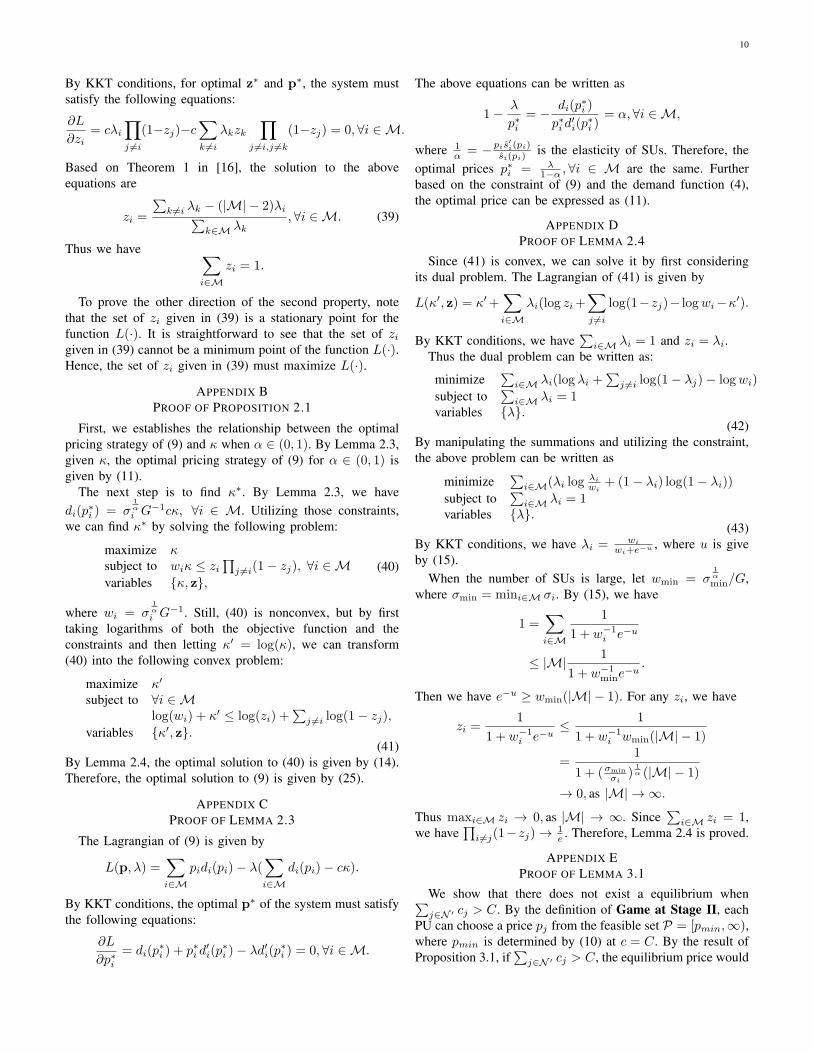
In Figure 7, we examine the convergence of spectrumopportunities in the case of four PUs and 200 SUs by usingAlgorithm 2. Here, we choose 𝛼 = 0.3 and 𝑎 = 30 suchthat 0 < �� ≤ 𝐶1−𝛼 and 𝑐𝐿 > 0.75. As illustrated in Figure7, the sum of initial normalized spectrum opportunities isgreater than 1, in which case there is no equilibrium pointbased on Lemma 3.1. Each PU then updates its offeredspectrum opportunity based on its current demand (this processcorresponds to the iterations from 1 to 3 in Figure 7). Oncethe total supply is within the feasible region, each PU adjustsits supply based on Proposition 3.2. Based on Proposition 3.3,there exists a unique equilibrium, which is verified in Figure7.

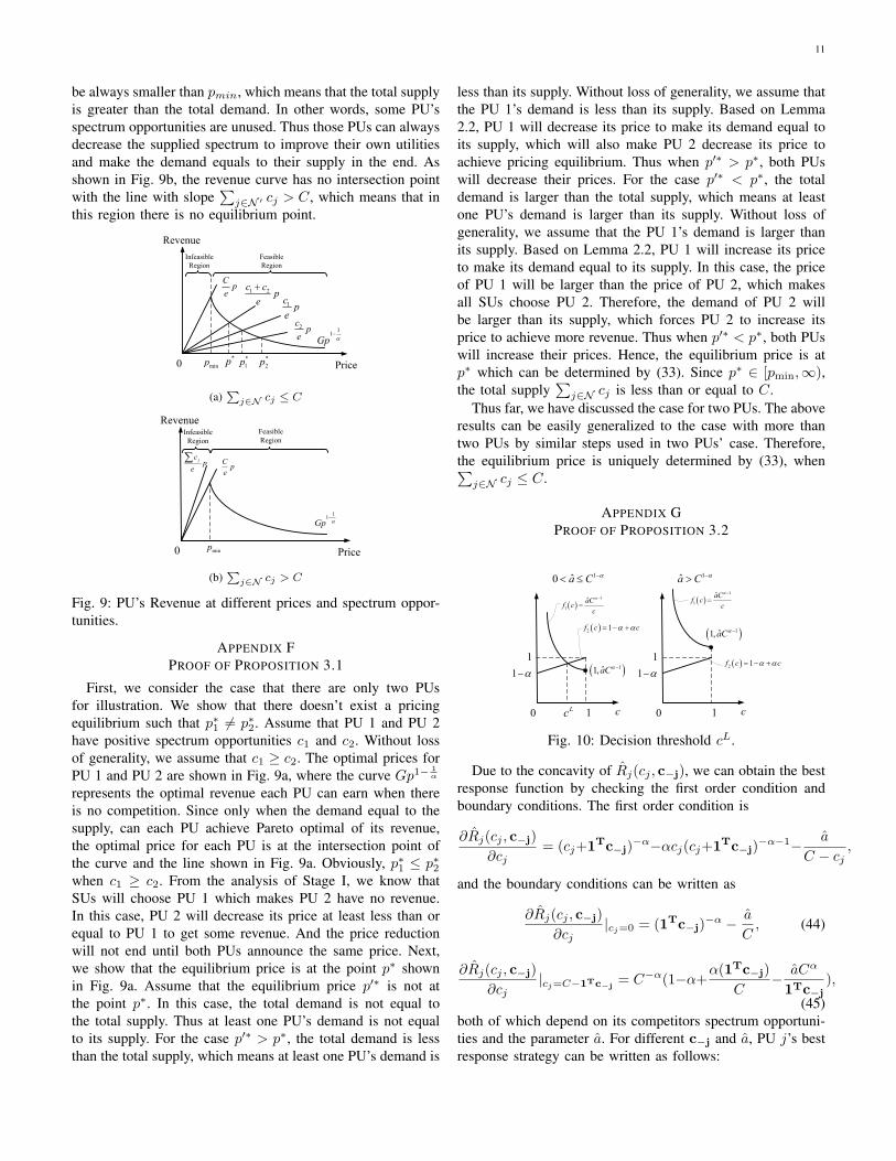
Figure 8 depicts how the equilibrium price evolves underdifferent elasticities of SUs and different numbers of PUs.Specifically, we choose 𝑎 = 30 and ∣ℳ∣ = 200. For each𝛼, the equilibrium price decreases with the number of PUs,due to more competition among PUs. In other words, SUs canbenefit from the competition among PUs. Moreover, it can beseen that the equilibrium price approaches 𝑝min as the numberof PUs increases.

IV. CONCLUSION

This paper studied pricing-based spectrum access controlin cognitive radio networks, where SUs contend for channelusage by random access when the PU’s channel is available.We studied two models: one with a monopoly PU market and

2 3 4 5 64.5

5

5.5

6

6.5

7

7.5

8

Number of PUs

Pric

ing

Equ

ilibr

ium

α=0.25,cL=0.96

α=0.30,cL=0.76

α=0.33,cL=0.67

Fig. 8: Price equilibrium corresponding to different elasticitiesof SUs and different numbers of PUs.

the other with a multiple PU market. For the monopoly PUmarket model, we used the revenue maximization approach tocharacterize the appropriate choice of flat and usage prices, anddeveloped a Pareto optimal solution, which was shown to benear-optimal. More importantly, this Pareto optimal solutionexhibits a decentralized structure, i.e., the Pareto optimalpricing strategy and access probabilities can be computed bythe PU and the SUs locally. We also analyzed a PU profitmaximization problem by examining the tradeoff between thePU’s utility and its revenue.

We then studied the competition of PUs in the multiplePU market by modeling the competition as a three-stageStackelberg game among PUs, in terms of access pricesand the offered spectrum opportunities. We showed that thenumber of equilibria has a threshold structure: if the numberof PUs is greater than the threshold, there exist infinitely manyequilibria, where the equilibrium price reduces to the minimumprice that may cut down PUs’ profit; otherwise, there exists aunique equilibrium. We further provided an iterative algorithmto find the equilibrium.

In this paper, we have studied thoroughly pricing-based dis-tributed spectrum access control for SUs, for the market modelwith homogeneous PUs. A natural next step is to explore themodel with heterogeneous PUs. Another interesting directionis to investigate transient behaviors corresponding to dynamicspectrum access, in the presence of spectrum hole dynamics.

ACKNOWLEDGMENT

We would like to thank Prashanth Hande for helpful com-ments and discussions.

APPENDIX APROOF OF LEMMA 2.2

The proof of the first property is contained in that ofthe second one. The second property can be derived fromthe Lagrangian of (8) by utilizing the KKT conditions. TheLagrangian of (8) is given by

𝐿(z,p, 𝜆) =∑𝑖∈ℳ

(𝑝𝑖 − 𝜆𝑖)𝑑𝑖(𝑝𝑖) + 𝑐∑𝑖∈ℳ

𝜆𝑖𝑧𝑖∏𝑗 ∕=𝑖

(1− 𝑧𝑗).

10

By KKT conditions, for optimal z∗ and p∗, the system mustsatisfy the following equations:

∂𝐿

∂𝑧𝑖= 𝑐𝜆𝑖

∏𝑗 ∕=𝑖

(1−𝑧𝑗)−𝑐∑𝑘 ∕=𝑖

𝜆𝑘𝑧𝑘∏

𝑗 ∕=𝑖,𝑗 ∕=𝑘

(1−𝑧𝑗) = 0,∀𝑖 ∈ ℳ.

Based on Theorem 1 in [16], the solution to the aboveequations are

𝑧𝑖 =

∑𝑘 ∕=𝑖 𝜆𝑘 − (∣ℳ∣ − 2)𝜆𝑖∑

𝑘∈ℳ 𝜆𝑘,∀𝑖 ∈ ℳ. (39)

Thus we have ∑𝑖∈ℳ

𝑧𝑖 = 1.

To prove the other direction of the second property, notethat the set of 𝑧𝑖 given in (39) is a stationary point for thefunction 𝐿(⋅). It is straightforward to see that the set of 𝑧𝑖given in (39) cannot be a minimum point of the function 𝐿(⋅).Hence, the set of 𝑧𝑖 given in (39) must maximize 𝐿(⋅).

APPENDIX BPROOF OF PROPOSITION 2.1

First, we establishes the relationship between the optimalpricing strategy of (9) and 𝜅 when 𝛼 ∈ (0, 1). By Lemma 2.3,given 𝜅, the optimal pricing strategy of (9) for 𝛼 ∈ (0, 1) isgiven by (11).

The next step is to find 𝜅∗. By Lemma 2.3, we have𝑑𝑖(𝑝

∗𝑖 ) = 𝜎

1𝛼𝑖 𝐺−1𝑐𝜅, ∀𝑖 ∈ ℳ. Utilizing those constraints,

we can find 𝜅∗ by solving the following problem:

maximize 𝜅subject to 𝑤𝑖𝜅 ≤ 𝑧𝑖

∏𝑗 ∕=𝑖(1− 𝑧𝑗), ∀𝑖 ∈ ℳ

variables {𝜅, z},(40)

where 𝑤𝑖 = 𝜎1𝛼𝑖 𝐺−1. Still, (40) is nonconvex, but by first

taking logarithms of both the objective function and theconstraints and then letting 𝜅′ = log(𝜅), we can transform(40) into the following convex problem:

maximize 𝜅′

subject to ∀𝑖 ∈ ℳlog(𝑤𝑖) + 𝜅′ ≤ log(𝑧𝑖) +

∑𝑗 ∕=𝑖 log(1− 𝑧𝑗),

variables {𝜅′, z}.(41)

By Lemma 2.4, the optimal solution to (40) is given by (14).Therefore, the optimal solution to (9) is given by (25).

APPENDIX CPROOF OF LEMMA 2.3

The Lagrangian of (9) is given by

𝐿(p, 𝜆) =∑𝑖∈ℳ

𝑝𝑖𝑑𝑖(𝑝𝑖)− 𝜆(∑𝑖∈ℳ

𝑑𝑖(𝑝𝑖)− 𝑐𝜅).

By KKT conditions, the optimal p∗ of the system must satisfythe following equations:

∂𝐿

∂𝑝∗𝑖= 𝑑𝑖(𝑝

∗𝑖 ) + 𝑝∗𝑖 𝑑

′𝑖(𝑝

∗𝑖 )− 𝜆𝑑′𝑖(𝑝

∗𝑖 ) = 0,∀𝑖 ∈ ℳ.

The above equations can be written as

1− 𝜆

𝑝∗𝑖= − 𝑑𝑖(𝑝

∗𝑖 )

𝑝∗𝑖 𝑑′𝑖(𝑝

∗𝑖 )

= 𝛼, ∀𝑖 ∈ ℳ,

where 1𝛼 = −𝑝𝑖𝑠

′𝑖(𝑝𝑖)

𝑠𝑖(𝑝𝑖)is the elasticity of SUs. Therefore, the

optimal prices 𝑝∗𝑖 = 𝜆1−𝛼 ,∀𝑖 ∈ ℳ are the same. Further

based on the constraint of (9) and the demand function (4),the optimal price can be expressed as (11).

APPENDIX DPROOF OF LEMMA 2.4

Since (41) is convex, we can solve it by first consideringits dual problem. The Lagrangian of (41) is given by

𝐿(𝜅′, z) = 𝜅′+∑𝑖∈ℳ

𝜆𝑖(log 𝑧𝑖+∑𝑗 ∕=𝑖

log(1−𝑧𝑗)− log𝑤𝑖−𝜅′).

By KKT conditions, we have∑

𝑖∈ℳ 𝜆𝑖 = 1 and 𝑧𝑖 = 𝜆𝑖.Thus the dual problem can be written as:

minimize∑

𝑖∈ℳ 𝜆𝑖(log 𝜆𝑖 +∑

𝑗 ∕=𝑖 log(1− 𝜆𝑗)− log𝑤𝑖)

subject to∑

𝑖∈ℳ 𝜆𝑖 = 1variables {𝜆}.

(42)By manipulating the summations and utilizing the constraint,the above problem can be written as

minimize∑

𝑖∈ℳ(𝜆𝑖 log𝜆𝑖

𝑤𝑖+ (1− 𝜆𝑖) log(1− 𝜆𝑖))

subject to∑

𝑖∈ℳ 𝜆𝑖 = 1variables {𝜆}.

(43)By KKT conditions, we have 𝜆𝑖 =

𝑤𝑖

𝑤𝑖+𝑒−𝑢 , where 𝑢 is giveby (15).

When the number of SUs is large, let 𝑤min = 𝜎1𝛼

min/𝐺,where 𝜎min = min𝑖∈ℳ 𝜎𝑖. By (15), we have

1 =∑𝑖∈ℳ

1

1 + 𝑤−1𝑖 𝑒−𝑢

≤ ∣ℳ∣ 1

1 + 𝑤−1min𝑒

−𝑢.

Then we have 𝑒−𝑢 ≥ 𝑤min(∣ℳ∣ − 1). For any 𝑧𝑖, we have

𝑧𝑖 =1

1 + 𝑤−1𝑖 𝑒−𝑢

≤ 1

1 + 𝑤−1𝑖 𝑤min(∣ℳ∣ − 1)

=1

1 + (𝜎min

𝜎𝑖)

1𝛼 (∣ℳ∣ − 1)

→ 0, as ∣ℳ∣ → ∞.

Thus max𝑖∈ℳ 𝑧𝑖 → 0, as ∣ℳ∣ → ∞. Since∑

𝑖∈ℳ 𝑧𝑖 = 1,we have

∏𝑖 ∕=𝑗(1−𝑧𝑗) → 1

𝑒 . Therefore, Lemma 2.4 is proved.

APPENDIX EPROOF OF LEMMA 3.1

We show that there does not exist a equilibrium when∑𝑗∈𝒩 ′ 𝑐𝑗 > 𝐶. By the definition of Game at Stage II, each

PU can choose a price 𝑝𝑗 from the feasible set 𝒫 = [𝑝𝑚𝑖𝑛,∞),where 𝑝𝑚𝑖𝑛 is determined by (10) at 𝑐 = 𝐶. By the result ofProposition 3.1, if

∑𝑗∈𝒩 ′ 𝑐𝑗 > 𝐶, the equilibrium price would

11

be always smaller than 𝑝𝑚𝑖𝑛, which means that the total supplyis greater than the total demand. In other words, some PU’sspectrum opportunities are unused. Thus those PUs can alwaysdecrease the supplied spectrum to improve their own utilitiesand make the demand equals to their supply in the end. Asshown in Fig. 9b, the revenue curve has no intersection pointwith the line with slope

∑𝑗∈𝒩 ′ 𝑐𝑗 > 𝐶, which means that in

this region there is no equilibrium point.

minp

Infeasible

Region

Feasible

Region

0

Cp

e1c pe

*

1p

11

Gp !

*

2p

2c pe

1 2c cp

e

"

*p

(a)∑

𝑗∈𝒩 𝑐𝑗 ≤ 𝐶

minp

Infeasible

Region

Feasible

Region

0

Cp

e

11

Gp !

jcp

e

"

(b)∑

𝑗∈𝒩 𝑐𝑗 > 𝐶

Fig. 9: PU’s Revenue at different prices and spectrum oppor-tunities.

APPENDIX FPROOF OF PROPOSITION 3.1

First, we consider the case that there are only two PUsfor illustration. We show that there doesn’t exist a pricingequilibrium such that 𝑝∗1 ∕= 𝑝∗2. Assume that PU 1 and PU 2have positive spectrum opportunities 𝑐1 and 𝑐2. Without lossof generality, we assume that 𝑐1 ≥ 𝑐2. The optimal prices forPU 1 and PU 2 are shown in Fig. 9a, where the curve 𝐺𝑝1−

1𝛼

represents the optimal revenue each PU can earn when thereis no competition. Since only when the demand equal to thesupply, can each PU achieve Pareto optimal of its revenue,the optimal price for each PU is at the intersection point ofthe curve and the line shown in Fig. 9a. Obviously, 𝑝∗1 ≤ 𝑝∗2when 𝑐1 ≥ 𝑐2. From the analysis of Stage I, we know thatSUs will choose PU 1 which makes PU 2 have no revenue.In this case, PU 2 will decrease its price at least less than orequal to PU 1 to get some revenue. And the price reductionwill not end until both PUs announce the same price. Next,we show that the equilibrium price is at the point 𝑝∗ shownin Fig. 9a. Assume that the equilibrium price 𝑝′∗ is not atthe point 𝑝∗. In this case, the total demand is not equal tothe total supply. Thus at least one PU’s demand is not equalto its supply. For the case 𝑝′∗ > 𝑝∗, the total demand is lessthan the total supply, which means at least one PU’s demand is

less than its supply. Without loss of generality, we assume thatthe PU 1’s demand is less than its supply. Based on Lemma2.2, PU 1 will decrease its price to make its demand equal toits supply, which will also make PU 2 decrease its price toachieve pricing equilibrium. Thus when 𝑝′∗ > 𝑝∗, both PUswill decrease their prices. For the case 𝑝′∗ < 𝑝∗, the totaldemand is larger than the total supply, which means at leastone PU’s demand is larger than its supply. Without loss ofgenerality, we assume that the PU 1’s demand is larger thanits supply. Based on Lemma 2.2, PU 1 will increase its priceto make its demand equal to its supply. In this case, the priceof PU 1 will be larger than the price of PU 2, which makesall SUs choose PU 2. Therefore, the demand of PU 2 willbe larger than its supply, which forces PU 2 to increase itsprice to achieve more revenue. Thus when 𝑝′∗ < 𝑝∗, both PUswill increase their prices. Hence, the equilibrium price is at𝑝∗ which can be determined by (33). Since 𝑝∗ ∈ [𝑝min,∞),the total supply

∑𝑗∈𝒩 𝑐𝑗 is less than or equal to 𝐶.

Thus far, we have discussed the case for two PUs. The aboveresults can be easily generalized to the case with more thantwo PUs by similar steps used in two PUs’ case. Therefore,the equilibrium price is uniquely determined by (33), when∑

𝑗∈𝒩 𝑐𝑗 ≤ 𝐶.

APPENDIX GPROOF OF PROPOSITION 3.2

Lc c0

!1ˆ1,aC"#

!1

1

aCf c

c

"#

$

1 "#

1

1

!21f c c" "$ # %

c0

1 "#

1

1

!21f c c" "$ # %

1ˆ0 a C "#& ' 1a C "#(

!1

1

aCf c

c

"#

$

!1ˆ1,aC" #

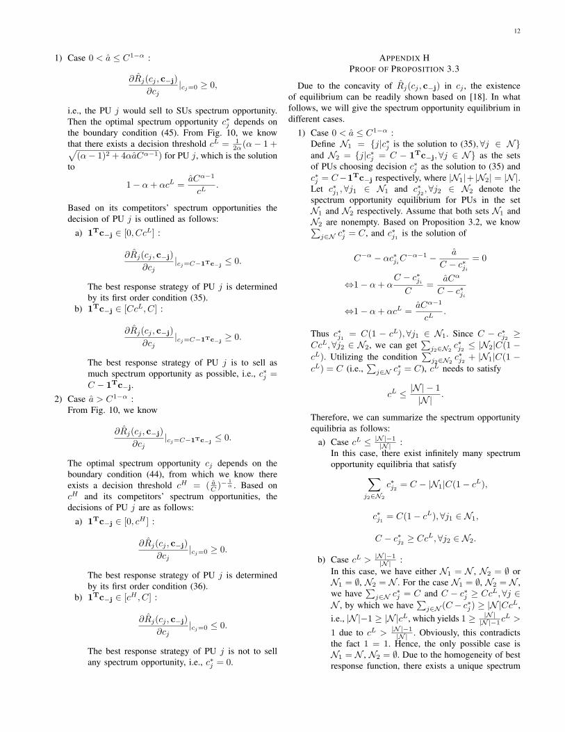
Fig. 10: Decision threshold 𝑐𝐿.

Due to the concavity of ��𝑗(𝑐𝑗 , c−j), we can obtain the bestresponse function by checking the first order condition andboundary conditions. The first order condition is

∂��𝑗(𝑐𝑗 , c−j)

∂𝑐𝑗= (𝑐𝑗+1Tc−j)

−𝛼−𝛼𝑐𝑗(𝑐𝑗+1Tc−j)−𝛼−1− ��

𝐶 − 𝑐𝑗,

and the boundary conditions can be written as

∂��𝑗(𝑐𝑗 , c−j)

∂𝑐𝑗∣𝑐𝑗=0 = (1Tc−j)

−𝛼 − ��

𝐶, (44)

∂��𝑗(𝑐𝑗 , c−j)

∂𝑐𝑗∣𝑐𝑗=𝐶−1Tc−j

= 𝐶−𝛼(1−𝛼+𝛼(1Tc−j)

𝐶− ��𝐶𝛼

1Tc−j),

(45)both of which depend on its competitors spectrum opportuni-ties and the parameter ��. For different c−j and ��, PU 𝑗’s bestresponse strategy can be written as follows:

12

1) Case 0 < �� ≤ 𝐶1−𝛼 :

∂��𝑗(𝑐𝑗 , c−j)

∂𝑐𝑗∣𝑐𝑗=0 ≥ 0,

i.e., the PU 𝑗 would sell to SUs spectrum opportunity.Then the optimal spectrum opportunity 𝑐∗𝑗 depends onthe boundary condition (45). From Fig. 10, we knowthat there exists a decision threshold 𝑐𝐿 = 1

2𝛼 (𝛼− 1 +√(𝛼− 1)2 + 4𝛼��𝐶𝛼−1) for PU 𝑗, which is the solution

to

1− 𝛼+ 𝛼𝑐𝐿 =��𝐶𝛼−1

𝑐𝐿.

Based on its competitors’ spectrum opportunities thedecision of PU 𝑗 is outlined as follows:

a) 1Tc−j ∈ [0, 𝐶𝑐𝐿] :

∂��𝑗(𝑐𝑗 , c−j)

∂𝑐𝑗∣𝑐𝑗=𝐶−1Tc−j

≤ 0.

The best response strategy of PU 𝑗 is determinedby its first order condition (35).

b) 1Tc−j ∈ [𝐶𝑐𝐿, 𝐶] :

∂��𝑗(𝑐𝑗 , c−j)

∂𝑐𝑗∣𝑐𝑗=𝐶−1Tc−j

≥ 0.

The best response strategy of PU 𝑗 is to sell asmuch spectrum opportunity as possible, i.e., 𝑐∗𝑗 =𝐶 − 1Tc−j.

2) Case �� > 𝐶1−𝛼 :From Fig. 10, we know

∂��𝑗(𝑐𝑗 , c−j)

∂𝑐𝑗∣𝑐𝑗=𝐶−1Tc−j

≤ 0.

The optimal spectrum opportunity 𝑐𝑗 depends on theboundary condition (44), from which we know thereexists a decision threshold 𝑐𝐻 = ( ��

𝐶 )−1𝛼 . Based on

𝑐𝐻 and its competitors’ spectrum opportunities, thedecisions of PU 𝑗 are as follows:

a) 1Tc−j ∈ [0, 𝑐𝐻 ] :

∂��𝑗(𝑐𝑗 , c−j)

∂𝑐𝑗∣𝑐𝑗=0 ≥ 0.

The best response strategy of PU 𝑗 is determinedby its first order condition (36).

b) 1Tc−j ∈ [𝑐𝐻 , 𝐶] :

∂��𝑗(𝑐𝑗 , c−j)

∂𝑐𝑗∣𝑐𝑗=0 ≤ 0.

The best response strategy of PU 𝑗 is not to sellany spectrum opportunity, i.e., 𝑐∗𝑗 = 0.

APPENDIX HPROOF OF PROPOSITION 3.3

Due to the concavity of ��𝑗(𝑐𝑗 , c−j) in 𝑐𝑗 , the existenceof equilibrium can be readily shown based on [18]. In whatfollows, we will give the spectrum opportunity equilibrium indifferent cases.

1) Case 0 < �� ≤ 𝐶1−𝛼 :Define 𝒩1 = {𝑗∣𝑐∗𝑗 is the solution to (35),∀𝑗 ∈ 𝒩}and 𝒩2 = {𝑗∣𝑐∗𝑗 = 𝐶 − 1Tc−j,∀𝑗 ∈ 𝒩} as the setsof PUs choosing decision 𝑐∗𝑗 as the solution to (35) and𝑐∗𝑗 = 𝐶−1Tc−j respectively, where ∣𝒩1∣+ ∣𝒩2∣ = ∣𝒩 ∣.Let 𝑐∗𝑗1 ,∀𝑗1 ∈ 𝒩1 and 𝑐∗𝑗2 ,∀𝑗2 ∈ 𝒩2 denote thespectrum opportunity equilibrium for PUs in the set𝒩1 and 𝒩2 respectively. Assume that both sets 𝒩1 and𝒩2 are nonempty. Based on Proposition 3.2, we know∑

𝑗∈𝒩 𝑐∗𝑗 = 𝐶, and 𝑐∗𝑗1 is the solution of

𝐶−𝛼 − 𝛼𝑐∗𝑗𝑖𝐶−𝛼−1 − ��

𝐶 − 𝑐∗𝑗𝑖= 0

⇔1− 𝛼+ 𝛼𝐶 − 𝑐∗𝑗𝑖

𝐶=

��𝐶𝛼

𝐶 − 𝑐∗𝑗𝑖

⇔1− 𝛼+ 𝛼𝑐𝐿 =��𝐶𝛼−1

𝑐𝐿.

Thus 𝑐∗𝑗1 = 𝐶(1 − 𝑐𝐿),∀𝑗1 ∈ 𝒩1. Since 𝐶 − 𝑐∗𝑗2 ≥𝐶𝑐𝐿,∀𝑗2 ∈ 𝒩2, we can get

∑𝑗2∈𝒩2

𝑐∗𝑗2 ≤ ∣𝒩2∣𝐶(1 −𝑐𝐿). Utilizing the condition

∑𝑗2∈𝒩2

𝑐∗𝑗2 + ∣𝒩1∣𝐶(1 −𝑐𝐿) = 𝐶 (i.e.,

∑𝑗∈𝒩 𝑐∗𝑗 = 𝐶), 𝑐𝐿 needs to satisfy

𝑐𝐿 ≤ ∣𝒩 ∣ − 1

∣𝒩 ∣ .

Therefore, we can summarize the spectrum opportunityequilibria as follows:

a) Case 𝑐𝐿 ≤ ∣𝒩 ∣−1∣𝒩 ∣ :

In this case, there exist infinitely many spectrumopportunity equilibria that satisfy∑

𝑗2∈𝒩2

𝑐∗𝑗2 = 𝐶 − ∣𝒩1∣𝐶(1− 𝑐𝐿),

𝑐∗𝑗1 = 𝐶(1− 𝑐𝐿),∀𝑗1 ∈ 𝒩1,

𝐶 − 𝑐∗𝑗2 ≥ 𝐶𝑐𝐿,∀𝑗2 ∈ 𝒩2.

b) Case 𝑐𝐿 > ∣𝒩 ∣−1∣𝒩 ∣ :

In this case, we have either 𝒩1 = 𝒩 , 𝒩2 = ∅ or𝒩1 = ∅, 𝒩2 = 𝒩 . For the case 𝒩1 = ∅, 𝒩2 = 𝒩 ,we have

∑𝑗∈𝒩 𝑐∗𝑗 = 𝐶 and 𝐶 − 𝑐∗𝑗 ≥ 𝐶𝑐𝐿,∀𝑗 ∈

𝒩 , by which we have∑

𝑗∈𝒩 (𝐶 − 𝑐∗𝑗 ) ≥ ∣𝒩 ∣𝐶𝑐𝐿,i.e., ∣𝒩 ∣−1 ≥ ∣𝒩 ∣𝑐𝐿, which yields 1 ≥ ∣𝒩 ∣

∣𝒩∣−1𝑐𝐿 >

1 due to 𝑐𝐿 > ∣𝒩 ∣−1∣𝒩 ∣ . Obviously, this contradicts

the fact 1 = 1. Hence, the only possible case is𝒩1 = 𝒩 , 𝒩2 = ∅. Due to the homogeneity of bestresponse function, there exists a unique spectrum

13

opportunity equilibrium [21], i.e., 𝑐∗𝑗 = 𝑐∗,∀𝑗 ∈𝒩 , where 𝑐∗ is the solution to

(∣𝒩 ∣𝑐∗)−𝛼 − 𝛼𝑐∗(∣𝒩 ∣𝑐∗)−𝛼−1 =��

𝐶 − 𝑐∗.

2) Case �� > 𝐶1−𝛼 :Define 𝒩1 = {𝑗∣𝑐∗𝑗 is the solution to (36),∀𝑗 ∈ 𝒩}and 𝒩2 = {𝑗∣𝑐∗𝑗 = 0,∀𝑗 ∈ 𝒩} as the sets of PUschoosing decision 𝑐∗𝑗 as the solution to (36) and 𝑐∗𝑗 = 0respectively, where ∣𝒩1∣+∣𝒩2∣ = ∣𝒩 ∣. Let 𝑐∗𝑗1 ,∀𝑗1 ∈ 𝒩1

and 𝑐∗𝑗2 ,∀𝑗2 ∈ 𝒩2 denote the spectrum opportunityequilibrium for PUs in the set 𝒩1 and 𝒩2 respectively.Based on Proposition 3.2, we know that 𝑐∗𝑗2 = 0, and wecan use (36) to calculate 𝑐∗𝑗1 . Then 𝑐∗𝑗1 = 𝑐∗,∀𝑗1 ∈ 𝒩1,where 𝑐∗ is the solution to

(∣𝒩1∣𝑐∗)−𝛼 − 𝛼𝑐∗(∣𝒩1∣𝑐∗)−𝛼−1 =��

𝐶 − 𝑐∗.

After some algebra, we have ∣𝒩1∣𝑐∗ < ( ��𝐶 )−

1𝛼 .

Since for each PU in 𝒩2, ∣𝒩1∣𝑐∗ < ( ��𝐶 )−

1𝛼 ,i.e.,

1Tc−j ∈ [0, 𝑐𝐻 ], the best response for PUs in 𝒩2 is thedecision (36), which shows that all PUs will choose thedecision (36). Due to the homogeneity of best responsefunction, there exists a unique spectrum opportunityequilibrium [21], which can be determined by (38).

REFERENCES

[1] X. Zhou and H. Zheng, “A general framework for truthful doublespectrum auctions,” in Proc. of IEEE INFOCOM, 2009.

[2] J. Jia, Q. Zhang, Q. Zhang, and M. Liu, “Revenue generation fortruthful spectrum auction in synamic spectrum access,” in Proc. of ACMMobiHoc, 2009.

[3] S. Sengupta, M. Chatterjee, and S. Ganguly, “An economic frameworkfor spectrum allocation and service pricing with competitive wirelesssevice providers,” in Proc. of IEEE DySPAN, 2007.

[4] K. Ryan, E. Arvantinos, and M. Buddhikot, “A new pricing model fornext generation spectrum access,” in Proc. of TAPAS, 2006.

[5] S. Gandhi, C. Buragohain, L. Cao, H. Zheng, and S. Suri, “Towardsreal-time dynamic spectrum auctions,” in Computer Networks, Vol. 52,Iss.5, pp. 879-897, 2008.

[6] Y. Wu, B. Wang, K. J. R. Liu, and T. C. Clancy, “A multi-winner cogni-tive spectrum auction framework with collusion-resistant mechanisms,”in Proc. of IEEE DySPAN, 2008.

[7] J. Huang, R. A. Berry, and M. L. Honig, “Auction-based spectrumsharing,” Mobile Networks and Applications, Vol. 11, pp. 405-418,Springer-Verlag, 2006.

[8] H. Mutlu, M. Alanyali, and D. Starobinski, “Spot pricing of secondaryspectrum usage in wireless cellular networks,” in Porc. of IEEE INFO-COM, 2008.

[9] Y. Xing, R. Chandramouli, and C. M. Cordeiro, “Price dynamics incompetitive agile spectrum access markets,” IEEE J. Selected Areas inComm., vol. 25, pp. 613-621, 2007.

[10] D. Niyato, E. Hossain, and Z. Han, “Dynamic spectrum access in IEEE802.22-based cognitive wireless networks: a game theoretic model forcompetitive spectrum bidding and pricing,” IEEE Wireless Communica-tions, vol. 16, no. 2, pp. 16-23, 2009.

[11] O. Ileri, D. Samardzija, T. Sizer, and N. B. Mandayam, “Demandresponsive pricing and competitive spectrum allocation via a spectrumserver,” in Proc. of IEEE DySPAN, 2005.

[12] D. Niyato, E. Hossain, and Z. Han, “Dynamics of multiple-seller andmultiple-buyer spectrum trading in cognitive radio networks: a game-theoretic modeling approach,” IEEE Trans. Mobile Computing, vol. 8,pp. 1009-1022, 2009.

[13] L. Duan, J. Huang, and B. Shou, “Cognitive mobile virtual networkoperator: investment and pricing with supply uncertainty,” in Proc. ofIEEE INFOCOM, 2010.

[14] D. Xu, X. Liu, and Z. Han, “A two-tier market for decentralized dynamicspectrum access in cognitive radio networks,” in Proc. of IEEE SECON,2010.

[15] P. Hande, M. Chiang, A. R. Calderbank, and J. Zhang, “Pricing underconstraints in access networks: revenue maximization and congestionmanagement,” in Proc. of IEEE INFOCOM, 2010.

[16] J. Sun and E. Modiano, ”Channel allocation using pricing in satellitenetworks,” Conference on Information Science and Systems (CISS),Princeton, NJ, March, 2006.

[17] A. Mas-Colell, M.D. Whinston, and J.R. Green, Microeconomic Theory,Oxford University Press, Oxford, United Kingdom, 1995.

[18] M. J. Osborne and A. Rubinstein, A Course In Game Theory. The MITPress, 1994.

[19] D. P. Bertsekas and R. Gallager, Date Networks. Prentice Hall, Engle-wood Cliffs, NJ, 1990.

[20] R. Knopp and P. A. Humblet, ”Information Capacity and power Controlin Single-Cell Multiuser Communications”, Int. Conf. on Communica-tions, Seattle, June 1995.

[21] D. Zheng, W. Ge, and J. Zhang, “Distributed Opportunistic SchedulingFor Ad-Hoc Networks With Random Access: An Optimal StoppingApproach,” IEEE Transactions on Information Theoryvol. 55, pp. 205-222, 2009.