Pricing Asian Options Using Monte Carlo - GitHub Pages · Pricing Asian Options Using Monte Carlo Joy Tolia 1. Contents 1 Introduction 2 ... The full set of results for each option

Pricing Asian Options Using Monte Carlo

Joy Tolia

1

Contents

1 Introduction 21.1 Implementation . . . . . . . . . . . . . . . . . . . . . . . . . . . . . . . . . . . . . . . 31.2 Types of Errors . . . . . . . . . . . . . . . . . . . . . . . . . . . . . . . . . . . . . . . 31.3 Error Analysis . . . . . . . . . . . . . . . . . . . . . . . . . . . . . . . . . . . . . . . 3

2 Model Error 42.1 Implementation . . . . . . . . . . . . . . . . . . . . . . . . . . . . . . . . . . . . . . . 42.2 Results . . . . . . . . . . . . . . . . . . . . . . . . . . . . . . . . . . . . . . . . . . . . 52.3 Conclusion . . . . . . . . . . . . . . . . . . . . . . . . . . . . . . . . . . . . . . . . . 5

3 Rate of Convergence 63.1 Implementation . . . . . . . . . . . . . . . . . . . . . . . . . . . . . . . . . . . . . . . 73.2 Results . . . . . . . . . . . . . . . . . . . . . . . . . . . . . . . . . . . . . . . . . . . . 73.3 Conclusion . . . . . . . . . . . . . . . . . . . . . . . . . . . . . . . . . . . . . . . . . 8

4 Size of Timestep δt 84.1 Implementation . . . . . . . . . . . . . . . . . . . . . . . . . . . . . . . . . . . . . . . 84.2 Results . . . . . . . . . . . . . . . . . . . . . . . . . . . . . . . . . . . . . . . . . . . . 94.3 Conclusion . . . . . . . . . . . . . . . . . . . . . . . . . . . . . . . . . . . . . . . . . 9

5 Multi Level Monte-Carlo 95.1 Methodology . . . . . . . . . . . . . . . . . . . . . . . . . . . . . . . . . . . . . . . . 95.2 Implementation . . . . . . . . . . . . . . . . . . . . . . . . . . . . . . . . . . . . . . . 105.3 Results & Conclusion . . . . . . . . . . . . . . . . . . . . . . . . . . . . . . . . . . . . 11

6 Appendix 126.1 Underlying Model . . . . . . . . . . . . . . . . . . . . . . . . . . . . . . . . . . . . . 126.2 Model Error Results . . . . . . . . . . . . . . . . . . . . . . . . . . . . . . . . . . . . 146.3 Rate of Convergence Results . . . . . . . . . . . . . . . . . . . . . . . . . . . . . . . 18

6.3.1 Arithmetic - Fixed Strike . . . . . . . . . . . . . . . . . . . . . . . . . . . . . 186.3.2 Arithmetic - Floating Strike . . . . . . . . . . . . . . . . . . . . . . . . . . . . 196.3.3 Geometric - Fixed Strike . . . . . . . . . . . . . . . . . . . . . . . . . . . . . . 196.3.4 Geometric - Floating Strike . . . . . . . . . . . . . . . . . . . . . . . . . . . . 20

6.4 Code . . . . . . . . . . . . . . . . . . . . . . . . . . . . . . . . . . . . . . . . . . . . . 206.4.1 Model Error Code . . . . . . . . . . . . . . . . . . . . . . . . . . . . . . . . . 206.4.2 Rate of Convergence Code . . . . . . . . . . . . . . . . . . . . . . . . . . . . . 236.4.3 Size of Timestep δt Code . . . . . . . . . . . . . . . . . . . . . . . . . . . . . 276.4.4 Multi Level Monte-Carlo . . . . . . . . . . . . . . . . . . . . . . . . . . . . . . 29

2

1 Introduction

• The objective of this assignment is to implement Monte-Carlo methods within Matlab toprice different Asian options and to compare the different results.

• I chose Matlab as I have used it before and I thought it would be interesting to find out howMonte-Carlo will behave in Matlab.

1.1 Implementation

• Matlab is very fast at doing array operations, much faster than using for loops. So I wantedto find a way to have as much of my implementation as possible using array operations.

• The problem becomes memory. I found that the computer could only handle arrays with 107

elements at once.

• First the decide the size δt and anything to do with averaging across time will be done witharray operations. Then using the information about my computer and its memory restrictions,I would do the averaging across samples in chunks. For examples if δt = 10−2 then I wouldchoose 105 for the number of samples in each chunk to average over.

• By doing this I am hoping to get the most of out Matlab in terms of speed.

1.2 Types of Errors

• There are 3 types of errors we would like to analyse; error from approximating the underlyingmodel, error from averaging over samples and error from size of the timestep δt.

• We will get error from approximating the underlying model as we will be comparing Euler-Maruyama and Milstein schemes. Note that for our underlying model we do have a closedform formula:

St+δt = Ste(r−σ2/2)δt+σφ

√δt, φ ∼ N (0, 1)

However, it will not always be the case where we will find a closed form solution for theunderlying.

• We will get error from averaging over samples which is the main error in Monte-Carlo methodsand will be looking at the antithetics scheme to see how they affect the number of samplesneeded to get an accurate answer.

• We will assume we want to price continuous Asian options hence our δt→ 0, however we willhave to take δt > 0 for example δt = 0.01 which will give us an error from averaging overtime.

1.3 Error Analysis

• Having spent quite a while trying to work out the best way to present results, the hardestpart was to assume we didn’t have exact solutions and to have a way to working out if thesolution converged or not.

3

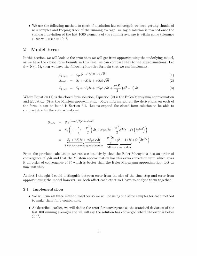
• We use the following method to check if a solution has converged; we keep getting chunks ofnew samples and keeping track of the running average. we say a solution is reached once thestandard deviation of the last 1000 elements of the running average is within some toleranceε. we will use ε = 10−5.

2 Model Error

In this section, we will look at the error that we will get from approximating the underlying model,as we have the closed form formula in this case, we can compare that to the approximations. Letφ ∼ N (0, 1), then we have the following iterative formula that we can implement:


√δt (1)

St+δt = St + rStδt+ σStφ√δt (2)

St+δt = St + rStδt+ σStφ√δt+

σ2St2

(φ2 − 1

)δt (3)

Where Equation (1) is the closed form solution, Equation (2) is the Euler-Maruyama approximationand Equation (3) is the Milstein approximation. More information on the derivations on each ofthe formula can be found is Section 6.1. Let us expand the closed form solution to be able tocompare it with the approximations:


√δt

= St

(1 +

(r − σ2

2

)δt+ σφ

√δt+

σ2

2φ2δt+O

(δt3/2

))= St + rStδt+ σStφ

√δt︸︷︷︸

Euler-Maruyama approximation

+σ2St

2

(φ2 − 1

)δt︸︷︷︸

Miltstein correction

+O(δt3/2

)

From the previous calculation we can see intuitively that the Euler-Maruyama has an order ofconvergence of

√δt and that the Milstein approximation has this extra correction term which gives

it an order of convergence of δt which is better than the Euler-Maruyama approximation. Let usnow test this.

At first I thought I could distinguish between error from the size of the time step and error fromapproximating the model however, we both affect each other so I have to analyse them together.

2.1 Implementation

• We will run all three method together so we will be using the same samples for each methodto make them fully comparable.

• As described earlier, we will define the error for convergence as the standard deviation of thelast 100 running averages and we will say the solution has converged where the error is below10−3.

4

• In this case, we will take the maximum standard deviation of all three methods so eachmethod will have the same number of samples in the end.

• All the code used in this section can be found in Section 1 within the Code document.

• We define the error for the different methods as the absolute difference between the convergedsolution of Euler-Maruyama (Equation (2)) and Milstein (Equation (3)) method versus thebenchmark case of the closed form (Equation (1)).

2.2 Results

The full set of results for each option can be found in Section 6.2. The following are the results forthe arithmetic fixed strike Asian call and put options:

δt10−1 10−2 10−3 10−4 10−5

Euler-Maruyama 0.0088 5.6402×10−4 2.9598×10−4 4.3800×10−5 3.3715×10−5

Milstein 0.0233 0.0026 2.5500×10−4 2.5847×10−5 2.5360×10−6

Table 1: Error from the benchmark closed form solution for the arithmetic fixed strike Asian calloption

δt10−1 10−2 10−3 10−4 10−5

Euler-Maruyama 3.3435×10−4 9.5593×10−4 1.1241×10−4 6.3920×10−5 3.7049×10−5

Milstein 0.0184 0.0019 1.9486×10−4 1.9174×10−5 1.9412×10−6

Table 2: Error from the benchmark closed form solution for the arithmetic fixed strike Asian putoption

Figure 1: Error from the benchmark closed formsolution for the arithmetic fixed strike Asian calloption

Figure 2: Error from the benchmark closed formsolution for the arithmetic fixed strike Asian putoption

5

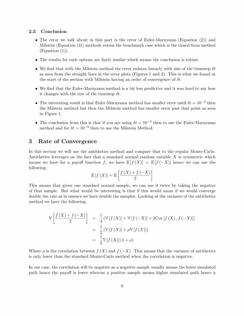
2.3 Conclusion

• The error we talk about in this part is the error of Euler-Maruyama (Equation (2)) andMilstein (Equation (3)) methods versus the benchmark case which is the closed form method(Equation (1)).

• The results for each options are fairly similar which means the conclusion is robust.

• We find that with the Milstein method the error reduces linearly with size of the timestep δtas seen from the straight lines in the error plots (Figures 1 and 2). This is what we found atthe start of the section with Milstein having an order of convergence of δt.

• We find that the Euler-Maruyama method is a bit less predictive and it was hard to say howit changes with the size of the timestep δt.

• The interesting result is that Euler-Maruyama method has smaller error until δt = 10−3 thenthe Milstein method but then the Milstein method has smaller error past that point as seenin Figure 1.

• The conclusion from this is that if you are using δt < 10−3 then to use the Euler-Maruyamamethod and for δt > 10−3 then to use the Milstein Method.

3 Rate of Convergence

In this section we will use the antithetics method and compare that to the regular Monte-Carlo.Antithetics leverages on the fact that a standard normal random variable X is symmetric whichmeans we have for a payoff function f , we have E [f (X)] = E [f (−X)] hence we can use thefollowing:

E [f (X)] = E[f (X) + f (−X)

2

]This means that given one standard normal sample, we can use it twice by taking the negativeof that sample. But what would be interesting is that if this would mean if we would convergedouble the rate as in essence we have double the samples. Looking at the variance of the antitheticsmethod we have the following:

V[f (X) + f (−X)

2

]=

1

4(V [f (X)] + V [f (−X)] + 2Cov [f (X) , f (−X)])

=1

2(V [f (X)] + ρV [f (X)])

=1

2V [f (X)] (1 + ρ)

Where ρ is the correlation between f (X) and f (−X). This means that the variance of antitheticsis only lower than the standard Monte-Carlo method when the correlation is negative.

In our case, the correlation will be negative as a negative sample usually means the lower simulatedpath hence the payoff is lower whereas a positive sample means higher simulated path hence a

6

higher payoff.

We have calculated the correlations between the payoffs from samples and their negative equivalentsfor 104 samples with δt = 10−3 to get an understanding:

Call PutArith Geom Arith Geom

Fix Float Fix Float Fix Float Fix Float

ρ -0.52 -0.48 -0.51 -0.47 -0.41 -0.44 -0.41 -0.43

Table 3: Correlations between the payoffs of 10−4 samples and their negative equivalents withδt = 10−3

From this we can see that the call options has a more negative correlation than the put options.So we should see that the call options should converge faster than the put options. Also no notethat as ρ ≈ −0.5, we would have quartered the variance hence halved the standard deviation forthese options.

3.1 Implementation

• We will use the same definition of convergence error as before but we will use the standarddeviation of the last 1000 running averages from Monte Carlo. We say that we have convergedto a solution when this error is less than 10−4.

• We will keep the size of the timestep δt constant at 10−3 as we are analysing the rate ofconvergence more than the accuracy of the results.

• We will use the Milstein method to model the underlying.

• All the code used in this section can be found in Section 2 within the Code document.

3.2 Results

The full set of results can be found in Section 6.3. Here are the results for the arithmetic fixedstrike Asian options:

Call Put

Standard Antithetic Standard Antithetic

Final Value 5.7616 5.7654 3.3468 3.3462

Final Error (×10−6) 9.9 7.7 9.7 8.2

Samples (×105) 42.4 15.2 30.4 12.8

Time (seconds) 253 154 124 91

Table 4: Data for the arithmetic fixed strike Asian options

7

Figure 3: Convergence error measure for thearithmetic fixed strike Asian call option

Figure 4: Convergence error measure for thearithmetic fixed strike Asian put option

3.3 Conclusion

• We find similar results across all options which again shows that we can interpret our resultswith confidence.

• We see that the antithetics method works very well from our results, as seen in Figures 3 and4.

• We see that the number of samples needed to achieve convergence have more than halved asexpected as seen in Table 4.

• We also find that the antithetics method works slightly better on call options than the putoptions as hypothesised earlier.

4 Size of Timestep δt

In this section, we will analyse how the size of the timestep affects accuracy of the results.

4.1 Implementation

• We will use the closed form solution for the underlying as we want to get rid of the error fromapproximating the underlying.

• We will only work with one option in this case which is the geometric fixed strike Asian calloption and assume that the exact solution is 5.5468 which is from [1].

• Once the solution has converged, we will compared the converged solution with the exactsolution and look at the absolute difference between the two and use that as our error.

• All the code for this part can be found in Section 3 of the code document.

8

4.2 Results

Figure 5: Error of converged solution versus the exact solution for different timesteps

4.3 Conclusion

• Having run this several times and getting results similar to Figure 5, we conclude that theresults are weak and hard to interpret.

• We would have expected the error to reduce as δt went down. However, the error from Monte-Carlo of using random samples might outweigh the error from the timestep δt making it hardto see the affect of δt on the accuracy of the results.

5 Multi Level Monte-Carlo

In summer 2015, I did a research project under a supervisor where we will looking at calculatingvalues for stochastic integrals. One of the papers I came across was [2] on Multi Level Monte-Carlowhich looked very interesting as it has a lower computational complexity than the standard Monte-Carlo but I never got to implement it. I have taken the chance in this assignment to implementthe algorithm.

5.1 Methodology

Consider Monte Carlo path simulations with different timesteps hl = M−lT , l = 0, 1, . . . , L. LetP denote the discounted risk neutral payoff and Pl denote approximations of P using a numericaldiscretisation with timestep hl. We have:

E[PL

]= E

[P0

]+

L∑l=1

E[Pl − Pl−1

]

9

Let Y0 be the estimator for E[P0

]using N0 samples and Yl, for l > 0, be the estimator for

E[Pl − Pl−1

]using Nl samples. For us it is:

Y0 =1

N0

N0∑i=1

P(i)0

Yl =1

Nl

Nl∑i=1

(P

(i)l − P

(i)l−1

), l > 0

The key point here is that the quantity P(i)l − P

(i)l−1 comes from two discrete approx-

imations with different timesteps but the same Brownian motion which reduces thevariance. This is easily implemented by first constructing the Brownian increments for the simu-

lation of the discrete path leading to the evaluation of P(i)l and then summing them in groups of

M to give discrete Brownian increments for the evaluation of P(i)l−1.

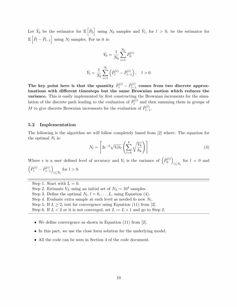
5.2 Implementation

The following is the algorithm we will follow completely based from [2] where: The equation forthe optimal Nl is:

Nl =

⌈2ε−2

√Vlhl

(k∑l=0

√Vkhk

)⌉(4)

Where ε is a user defined level of accuracy and Vl is the variance of(P

(i)0

)i≤Nl

for l = 0 and(P

(i)l − P

(i)l−1

)i≤Nl

for l > 0.

Step 1. Start with L = 0.Step 2. Estimate VL using an initial set of NL = 104 samples.Step 3. Define the optimal Nl, l = 0, . . . , L, using Equation (4).Step 4. Evaluate extra sample at each level as needed fo new Nl.Step 5. If L ≥ 2, test for convergence using Equation (11) from [2].Step 6. If L < 2 or it is not converged, set L := L+ 1 and go to Step 2.

• We define convergence as shown in Equation (11) from [2].

• In this part, we use the close form solution for the underlying model.

• All the code can be seen in Section 4 of the code document.

10

5.3 Results & Conclusion

Figure 6: Value from Multi Level Monte-Carlo with increasing levels

• The code ran in less than two seconds due to the vectorisation from Matlab and as thealgorithm works well.

• Accuracy was set to ε = 0.01 which is fairly low. Even though Figure 6 shows very goodconvergence, that was for only one run, there is still error (as expected) from different runs.

• One problem currently is when ε is increased, my computer cannot handle the sizes of ar-rays produced in the algorithm which can be tackled by using for loops rather than arrayoperations. However, speed will be lost in doing so.

• As each level greater than 0 is a difference between two discretisations, the variance is lowerbecause both discretisation uses the same Brownian paths, making this the principal reasonthat it is better than the standard Monte-Carlo.

11

6 Appendix

6.1 Underlying Model

The following is the stochastic process that we assume the underlying asset follows in a risk neutralworld:

dSt = rStdt+ σStdWt

where r, σ ∈ R and Wt = (Wt : t > 0) is a standard Brownian motion. In this case, we have a closedform solution for the St+δt. We get this by using Ito’s lemma on log (St):

d (log (St)) =∂

∂t(log (St)) dt+

∂

∂St(log (St)) dSt +

1

2

∂2

∂S2t

(log (St)) dS2t

=1

St(rStdt+ σStdWt)−

1

2S2t

σ2S2t dt

=

(r − σ2

2

)dt+ σdWt

Using the integral equivalent over a timestep δt of the above relation gives the following equation:

log (St+δt)− log (St) =

(r − σ2

2

)δt+ σ (Wt+δt −Wt)

Finally as (Wt+δt −Wt) ∼ N (0, δt), letting φ ∼ N (0, 1), we have the following:

St+δt = St exp

((r − σ2

2

)δt+ σφ

√δt

)(5)

This is what we would like to implement for the underlying model if we were pricing using Monte-Carlo methods. However, this could be computationally costly due to the exponential function andthe model could be more complex and might not have a closed form solution so there are otherschemes that we can use. Let us start with a more general model:

dSt = a (St, t) dt+ b (St, t) dWt

Now using the integral equivalence of the above formula:

St+δt = St +

∫ t+δt

ta (Ss, s) ds+

∫ t+δt

tb (Ss, s) dWs (6)

Using Ito’s for a (Ss, s) and b (Ss, s), we have the following:

a (Ss, s) = a (St, t) +

∫ s

t

(∂a

∂u(Su, u) + a (Su, u)

∂a

∂Su(Su, u) +

1

2b2 (Su, u)

∂2a

∂S2u

(Su, u)

)du+ · · ·

· · ·+∫ s

tb (Su, u)

∂a

∂Su(Su, u) dWu

Similarly:

12

b (Ss, s) = b (St, t) +

∫ s

t

(∂b

∂u(Su, u) + a (Su, u)

∂b

∂Su(Su, u) +

1

2b2 (Su, u)

∂2b

∂S2u

(Su, u)

)du+ · · ·

· · ·+∫ s

tb (Su, u)

∂b

∂Su(Su, u) dWu

Now we can sub in a (Su, u) = rSu and b (Su, u) = σSu to get the following:

∂a

∂u(Su, u) = 0,

∂a

∂Su(Su, u) = r,

∂2a

∂S2u

(Su, u) = 0

∂b

∂u(Su, u) = 0,

∂b

∂Su(Su, u) = σ,

∂2b

∂S2u

(Su, u) = 0

Therefore we get:

a (Ss, s) = rSt +

∫ s

tr2Sudu+

∫ s

trσSudWu

b (Ss, s) = σSt +

∫ s

trσSudu+

∫ s

tσ2SudWu

Finally subbing the above equation into Equation (6):

St+δt = St +

∫ t+δt

ta (Ss, s) ds+

∫ t+δt

tb (Ss, s) dWs

= St +

∫ t+δt

t

(rSt +

∫ s

tr2Sudu+

∫ s

trσSudWu

)ds+ · · ·

· · ·+∫ t+δt

t

(σSt +

∫ s

trσSudu+

∫ s

tσ2SudWu

)dWs

= St + rStδt+ σSt (Wt+δt −Wt) + · · ·

· · ·+∫ t+δt

t

∫ s

tr2Su duds︸︷︷︸

O(δt2)

+

∫ t+δt

t

∫ s

trσSu dWuds︸︷︷︸

O(δt3/2)

+ · · ·

· · ·+∫ t+δt

t

∫ s

trσSu dudWs︸︷︷︸

O(δt3/2)

+¯

∫ t+δt

t

∫ s

tσ2Su dWudWs︸︷︷︸

O(δt)

= St + rStδt+ σSt (Wt+δt −Wt) + σ2∫ t+δt

t

∫ s

tSudWudWs +O

(δt3/2

)Let focus on the integral from above:

13

σ2∫ t+δt

t

∫ s

tSudWudWs = σ2

∫ t+δt

tSt (Ws −Wt) dWs +O (δt)

= σ2St

∫ t+δt

tWsdWs︸︷︷︸

Using Ito’s =(W 2t+δt−W

2t −δt)/2

−σ2StWt (Wt+δt −Wt) +O (δt)

=σ2St

2

(W 2t+δt −W 2

t − δt+ 2W 2t − 2Wt+δtWt

)+O (δt)

=σ2St

2

((Wt+δt −Wt)

2 − δt)

+O (δt)

Therefore we have:

St+δt = St + rStδt+ σSt (Wt+δt −Wt) +σ2St

2

((Wt+δt −Wt)

2 − δt)

+O (δt)

Let φ ∼ N (0, 1) then:

St+δt ≈ St + rStδt+ σStφ√δt+

σ2St2

((φ√δt)2− δt

)= St + rStδt+ σStφ

√δt︸︷︷︸

Euler-Maruyama approximation

+σ2St

2

(φ2 − 1

)δt︸︷︷︸

Milstein Correction

6.2 Model Error Results

δt10−1 10−2 10−3 10−4 10−5

Euler-Maruyama 0.0088 5.6402×10−4 2.9598×10−4 4.3800×10−5 3.3715×10−5

Milstein 0.0233 0.0026 2.5500×10−4 2.5847×10−5 2.5360×10−6

Table 5: Error from the benchmark closed form solution for the arithmetic fixed strike Asian calloption

δt10−1 10−2 10−3 10−4 10−5

Euler-Maruyama 3.3435×10−4 9.5593×10−4 1.1241×10−4 6.3920×10−5 3.7049×10−5

Milstein 0.0184 0.0019 1.9486×10−4 1.9174×10−5 1.9412×10−6

Table 6: Error from the benchmark closed form solution for the arithmetic fixed strike Asian putoption

14

Figure 7: Error from the benchmark closed formsolution for the arithmetic fixed strike Asian calloption

Figure 8: Error from the benchmark closed formsolution for the arithmetic fixed strike Asian putoption

δt10−1 10−2 10−3 10−4 10−5

Euler-Maruyama 0.0042 1.1359×10−4 6.9972×10−4 7.7009×10−5 6.5832×10−5

Milstein 0.0254 0.0026 2.6492×10−4 2.6019×10−5 2.5930×10−6

Table 7: Error from the benchmark closed form solution for the arithmetic floating strike Asiancall option

δt10−1 10−2 10−3 10−4 10−5

Euler-Maruyama 0.0024 0.0012 5.6068×10−4 1.8113×10−5 4.9870×10−5

Milstein 0.0193 0.0020 1.9384×10−4 1.9620×10−5 1.9405×10−6

Table 8: Error from the benchmark closed form solution for the arithmetic floating strike Asianput option

15

Figure 9: Error from the benchmark closed formsolution for the arithmetic floating strike Asiancall option

Figure 10: Error from the benchmark closedform solution for the arithmetic floating strikeAsian put option

δt10−1 10−2 10−3 10−4 10−5

Euler-Maruyama 0.0045 0.0014 2.8011×10−4 8.6369×10−5 1.9019×10−5

Milstein 0.0227 0.0023 2.3528×10−4 2.3503×10−5 2.3423×10−6

Table 9: Error from the benchmark closed form solution for the geometric fixed strike Asian calloption

δt10−1 10−2 10−3 10−4 10−5

Euler-Maruyama 9.2513×10−5 0.0014 2.2584×10−4 7.5734×10−5 8.7579×10−6

Milstein 0.0197 0.0021 2.0697×10−4 2.0652×10−5 2.0156×10−6

Table 10: Error from the benchmark closed form solution for the geometric fixed strike Asian putoption

16

Figure 11: Error from the benchmark closedform solution for the geometric fixed strikeAsian call option

Figure 12: Error from the benchmark closedform solution for the geometric fixed strikeAsian put option

δt10−1 10−2 10−3 10−4 10−5

Euler-Maruyama 0.0070 1.1555×10−4 7.4598×10−5 2.5574×10−5 1.7367×10−5

Milstein 0.0276 0.0028 2.8532×10−4 2.8003×10−5 2.8098×10−6

Table 11: Error from the benchmark closed form solution for the geometric floating strike Asiancall option

δt10−1 10−2 10−3 10−4 10−5

Euler-Maruyama 0.0020 3.4913×10−4 7.7019×10−4 8.1794×10−5 3.4532×10−6

Milstein 0.0171 0.0018 1.8251×10−4 1.8463×10−5 1.8594×10−6

Table 12: Error from the benchmark closed form solution for the geometric floating strike Asianput option

17

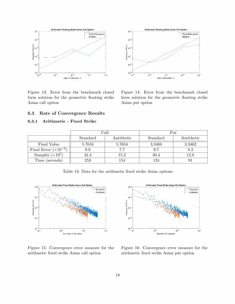
Figure 13: Error from the benchmark closedform solution for the geometric floating strikeAsian call option

Figure 14: Error from the benchmark closedform solution for the geometric floating strikeAsian put option

6.3 Rate of Convergence Results

6.3.1 Arithmetic - Fixed Strike

Call Put


Final Value 5.7616 5.7654 3.3468 3.3462

Final Error (×10−6) 9.9 7.7 9.7 8.2

Samples (×105) 42.4 15.2 30.4 12.8

Time (seconds) 253 154 124 91

Table 13: Data for the arithmetic fixed strike Asian options

Figure 15: Convergence error measure for thearithmetic fixed strike Asian call option

Figure 16: Convergence error measure for thearithmetic fixed strike Asian put option

18

6.3.2 Arithmetic - Floating Strike

Call Put


Final Value 5.8630 5.8589 3.4035 3.4027

Final Error (×10−6) 8.9 9.9 9.9 9.6

Samples (×105) 46.9 18.4 26.8 13.1

Time (seconds) 152 124 141 118

Table 14: Data for the arithmetic floating strike Asian options

Figure 17: Convergence error measure for thearithmetic floating strike Asian call option

Figure 18: Convergence error measure for thearithmetic floating strike Asian put option

6.3.3 Geometric - Fixed Strike

Call Put


Final Value 5.5445 5.5427 3.4652 3.4639

Final Error (×10−6) 9.9 9.8 9.8 5.7

Samples (×105) 35.5 17.9 24.2 14.2

Time (seconds) 271 243 149 149

Table 15: Data for the geometric fixed strike Asian options

19

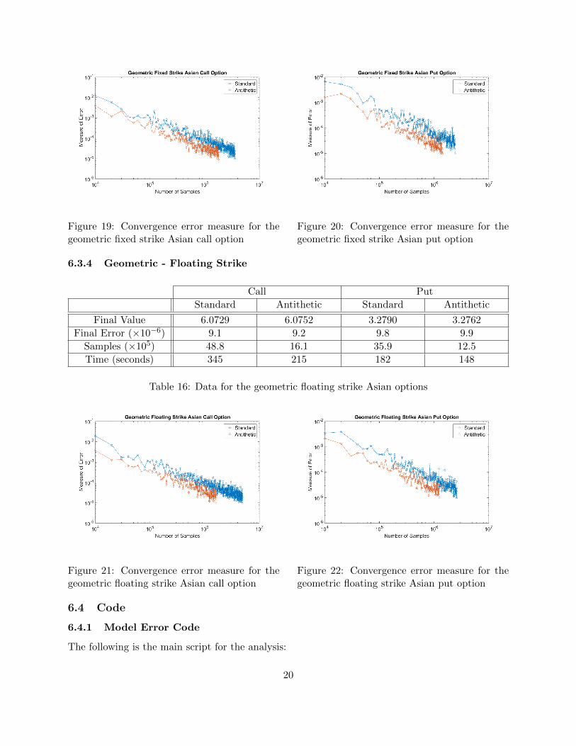
Figure 19: Convergence error measure for thegeometric fixed strike Asian call option

Figure 20: Convergence error measure for thegeometric fixed strike Asian put option

6.3.4 Geometric - Floating Strike

Call Put


Final Value 6.0729 6.0752 3.2790 3.2762

Final Error (×10−6) 9.1 9.2 9.8 9.9

Samples (×105) 48.8 16.1 35.9 12.5

Time (seconds) 345 215 182 148

Table 16: Data for the geometric floating strike Asian options

Figure 21: Convergence error measure for thegeometric floating strike Asian call option

Figure 22: Convergence error measure for thegeometric floating strike Asian put option

6.4 Code

6.4.1 Model Error Code

The following is the main script for the analysis:

20

1 % Data inputs2 T = 1;3 t = 0;4 S0 = 100;5 r = 0.05;6 K = 100;7 sigma = 0.2;8

9 % Accuracy Inputs10 dt = [1e−1 1e−2 1e−3 1e−4 1e−5];11 numSamples = 1e2;12 randseed = rng;13 eps = 1e−3;14

15 allError = zeros(2,length(dt));16 allTime = zeros(1,length(dt));17

18 % Loop through each timestep and calculate error19 for i = 1:length(dt)20 disp(['dt = ' num2str(dt(i))]);21 tic;22 [currentValue,currentSamples,errArray,sampleArray] =...23 modelMonteCarlo(dt(i),t,T,r,sigma,S0,K,randseed,eps,numSamples);24 allTime(i) = toc;25 allError(1,i) = abs(currentValue(1)−currentValue(2));26 allError(2,i) = abs(currentValue(1)−currentValue(3));27 disp(currentSamples);28 end29

30 %% Plotting31 figHandle = figure;32 set(figHandle,'Position',[20,20,1000,600])33

34 loglog(dt,allError(1,:),'−o',dt,allError(2,:),'−o');35

36

37 title('Geometric Floating Strike Asian Put Option')38 legend('Euler−Maruyama','Milstein')39 xlabel('Size of timestep \delta t')40 ylabel('Measure of Error')41 hold on;42

43 set(findall(figHandle,'−property','FontSize'),'FontSize',18)

The following is a function which runs the Monte-Carlo methods:

1 function [currentValue,currentSamples,errArray,sampleArray] =...2 modelMonteCarlo( dt, t, T, r, sigma, S0, K, randseed, eps ,numSamples)3 % Get the number of time periods needed4 numTimes = round((T−t)/dt) + 1;5 err = 100;6 rng(randseed);7 % Initialise arrays to hold information8 errArray1 = [];sampleArray1 = [];currentValue1 = 0;currentSamples1 = 0;

21

9 errArray2 = [];sampleArray2 = [];currentValue2 = 0;currentSamples2 = 0;10 errArray3 = [];sampleArray3 = [];currentValue3 = 0;currentSamples3 = 0;11 while err > eps12 % normal random samples13 phi = randn(numSamples,numTimes−1);14 % Use different formula to get each path15 % Closed form16 phi1 = exp((r−0.5*sigmaˆ2)*dt + sigma*phi*sqrt(dt));17 % Euler−Maruyama18 phi2 = 1 + r*dt + sigma*phi*sqrt(dt);19 % Milstein20 phi3 = 1 + (r+0.5*sigmaˆ2*(phi.ˆ2−1))*dt + sigma*phi*sqrt(dt);21 % Get paths for each formula22 S1 = S0*ones(numSamples,numTimes);23 S1(:,2:end) = S1(:,2:end).*cumprod(phi1,2);24 S2 = S0*ones(numSamples,numTimes);25 S2(:,2:end) = S2(:,2:end).*cumprod(phi2,2);26 S3 = S0*ones(numSamples,numTimes);27 S3(:,2:end) = S3(:,2:end).*cumprod(phi3,2);28 % Get values at the end of each path29 ST1 = S1(:,end);30 ST2 = S2(:,end);31 ST3 = S3(:,end);32 % Decide if arithmetic or geometric33 % S1 = mean(S1,2);34 % S2 = mean(S2,2);35 % S3 = mean(S3,2);36 S1 = exp(mean(log(S1),2));37 S2 = exp(mean(log(S2),2));38 S3 = exp(mean(log(S3),2));39 % Calculate the payoff and the error in the last 100 terms40 [err1,currentValue1,currentSamples1] = checkError(S1,ST1,K,r,T,t,...41 currentSamples1,currentValue1,numSamples);42 errArray1 = [errArray1 err1];43 sampleArray1 = [sampleArray1 currentSamples1];44 [err2,currentValue2,currentSamples2] = checkError(S2,ST2,K,r,T,t,...45 currentSamples2,currentValue2,numSamples);46 errArray2 = [errArray2 err2];47 sampleArray2 = [sampleArray2 currentSamples2];48 [err3,currentValue3,currentSamples3] = checkError(S3,ST3,K,r,T,t,...49 currentSamples3,currentValue3,numSamples);50 errArray3 = [errArray3 err3];51 sampleArray3 = [sampleArray3 currentSamples3];52 % Get the maximum error53 err = max([err1,err2,err3]);54 end55 % Store all the data56 currentSamples = [currentSamples1,currentSamples2,currentSamples3];57 currentValue = [currentValue1, currentValue2, currentValue3];58 errArray = [errArray1', errArray2', errArray3'];59 sampleArray = [sampleArray1', sampleArray2', sampleArray3'];60

61 end

The following is a function which calculates the running average from the new samples and getsthe convergence error:

22

1 function [err,currentValue,currentSamples] =...2 checkError(S,ST,K,r,T,t,currentSamples,currentValue,numSamples)3 % Check if this is the first calculation or not4 if currentSamples == 05 arraySamples = (currentSamples+1:currentSamples+numSamples)';6 payoffValue = exp(−r*(T−t))*optionPayoff(S,ST,K);7 else8 arraySamples = (currentSamples:currentSamples+numSamples)';9 payoffValue = [currentSamples*currentValue;...

10 exp(−r*(T−t))*optionPayoff(S,ST,K)];11 end12 % Calculate the cumulative mean13 meanValue = cumsum(payoffValue)./arraySamples;14 % Calculate the latest average15 currentValue = meanValue(end);16 currentSamples = currentSamples+numSamples;17 % Calculate the standard deviation of the last 1e3 averages18 err = std(meanValue(end−min(1e3,numSamples−1):end));19 end

The following is a function which calculate the payoff at maturity:

1 function [ P ] = optionPayoff( S, ST, K )2 % Payoff of the fixed strike call option3 P = max(S−K,0);4 % Payoff of the fixed strike put option5 % P = max(K−S,0);6 % Payoff of the floating strike call option7 % P = max(ST−S,0);8 % Payoff of the floating strike put option9 % P = max(S−ST,0);

10 end

6.4.2 Rate of Convergence Code


1 % Data inputs2 T = 1;3 t = 0;4 S0 = 100;5 r = 0.05;6 K = 100;7 sigma = 0.2;8 % Accuracy Inputs9 dt = 1e−3;

10 randseed = rng;11 % Run the standard Monte−Carlo12 tic;13 [standardCurrentValue,standardCurrentSamples,...14 standardErrArray,standardSampleArray] =...15 standardModelMonteCarlo(dt,t,T,r,sigma,S0,K,randseed);

23

16 standardTime = toc;17 % Run the antithetics Monte−Carlo18 tic;19 [antitheticCurrentValue,antitheticCurrentSamples,...20 antitheticErrArray,antitheticSampleArray] =...21 antitheticStandardModelMonteCarlo(dt,t,T,r,sigma,S0,K,randseed);22 antitheticTime = toc;23 %% Store Data24 allData = zeros(4,2);25 allData(:,1) = [standardCurrentValue;standardErrArray(end);...26 standardCurrentSamples;standardTime];27 allData(:,2) = [antitheticCurrentValue;antitheticErrArray(end);...28 antitheticCurrentSamples;antitheticTime];29 %% Plotting30 figHandle = figure;31 set(figHandle,'Position',[20,20,1000,600])32 loglog(standardSampleArray,standardErrArray,'−o',antitheticSampleArray,...33 antitheticErrArray,'−o');34 title('Arithmetic Floating Strike Asian Put Option')35 legend('Standard','Antithetic')36 xlabel('Number of Samples')37 ylabel('Measure of Error')38 hold on;39 set(findall(figHandle,'−property','FontSize'),'FontSize',18)

The following is a function which runs the standard Monte-Carlo method:

1 function [currentValue,currentSamples,errArray,sampleArray] = ...2 standardModelMonteCarlo(dt,t,T,r,sigma,S0,K,randseed)3 % Get the number of time periods needed4 numTimes = (T−t)/dt + 1;5 % Check is its an integer6 if rem(numTimes,1) ˜= 07 error('dt does not divide (T−t)');8 end9 % Initialise variables

10 numSamples = 1e4;11 currentValue = 0;12 currentSamples = 0;13 % Accurancy for the convergence14 eps = 1e−5;15 % Random seed16 rng(randseed);17 err = 100;18 errArray = [];19 sampleArray = [];20 % Run the while loop until convergence reached21 while err > eps22 % Get normal random samples23 phi = randn(numSamples,numTimes−1);24 % Get the Milstein method to calculate paths for the underlying25 phi = 1 + r*dt + phi*sqrt(dt)*sigma + 0.5*sigmaˆ2*(phi.ˆ2−1)*dt;26 % Calculate the paths of the underlying27 S = S0*ones(numSamples,numTimes);28 S(:,2:end) = S(:,2:end).*cumprod(phi,2);

24

29 % Calculate the end of each path30 ST = S(:,end);31 % Arithmetic or geometric sampling32 S = mean(S,2);33 % S = exp(mean(log(S),2));34 % Put everything together and check error35 [err,currentValue,currentSamples] =...36 checkError(S,ST,K,r,T,t,currentSamples,currentValue,numSamples);37 errArray = [errArray err];38 sampleArray = [sampleArray currentSamples];39 end40 end

The following is a function which runs the antithetic Monte-Carlo method:

1 function [currentValue,currentSamples,errArray,sampleArray] = ...2 antitheticStandardModelMonteCarlo(dt,t,T,r,sigma,S0,K,randseed)3 % Get the number of time periods needed4 numTimes = (T−t)/dt + 1;5 % Check is its an integer6 if rem(numTimes,1) ˜= 07 error('dt does not divide (T−t)');8 end9 % Initialise variables

10 numSamples = 1e4;11 currentValue = 0;12 currentSamples = 0;13 % Accurancy for the convergence14 eps = 1e−5;15 % Random seed16 rng(randseed);17 err = 100;18 errArray = [];19 sampleArray = [];20 % Run the while loop until convergence reached21 while err > eps22 % Get normal random samples23 phi = randn(numSamples,numTimes−1);24 % Adjust for calculate paths for the underlying using Milstein for25 % both positive and negative phi26 phiPos = 1 + r*dt + phi*sqrt(dt)*sigma + 0.5*sigmaˆ2*(phi.ˆ2−1)*dt;27 phiNeg = 1 + r*dt − phi*sqrt(dt)*sigma + 0.5*sigmaˆ2*(phi.ˆ2−1)*dt;28 % Calculate the paths of the underlying29 SPos = S0*ones(numSamples,numTimes);30 SPos(:,2:end) = SPos(:,2:end).*cumprod(phiPos,2);31 SNeg = S0*ones(numSamples,numTimes);32 SNeg(:,2:end) = SNeg(:,2:end).*cumprod(phiNeg,2);33 % Calculate the end of each path34 ST = zeros(2*numSamples,1);35 ST(1:2:2*numSamples−1) = SPos(:,end);36 ST(2:2:2*numSamples) = SNeg(:,end);37 % Arithmetic or geometric sampling38 SPos = mean(SPos,2);39 SNeg = mean(SNeg,2);40 % SPos = exp(mean(log(SPos),2));

25

41 % SNeg = exp(mean(log(SNeg),2));42 % Put everything together and check error43 S = zeros(2*numSamples,1);44 S(1:2:2*numSamples−1) = SPos;45 S(2:2:2*numSamples) = SNeg;46 [err,currentValue,currentSamples] = checkError(S,ST,K,r,T,t,...47 currentSamples,currentValue,2*numSamples);48 errArray = [errArray err];49 sampleArray = [sampleArray currentSamples];50 end51 % Half number of samples as antithetic52 sampleArray = sampleArray/2;53 currentSamples = currentSamples/2;54

55 end





1 function [ P ] = optionPayoff( S, ST, K )2 % Payoff of the fixed strike call option3 P = max(S−K,0);4 % Payoff of the fixed strike put option5 % P = max(K−S,0);6 % Payoff of the floating strike call option7 % P = max(ST−S,0);8 % Payoff of the floating strike put option9 % P = max(S−ST,0);

10 end

26

6.4.3 Size of Timestep δt Code


1 % Data inputs2 T = 1;3 t = 0;4 S0 = 100;5 r = 0.05;6 K = 100;7 sigma = 0.2;8 % Accuracy Inputs9 dt = [1e−1 1e−2 1e−3 1e−4 1e−5];

10 numSamples = 1e2;11 randseed = rng;12 eps = 1e−4;13 allError = zeros(1,length(dt));14 allTime = zeros(1,length(dt));15 currentValue = cell(1,length(dt));16 currentSamples = cell(1,length(dt));17 errArray = cell(1,length(dt));18 sampleArray = cell(1,length(dt));19 % Loop through each timestep and calculate error20 for i = 1:length(dt)21 disp(['dt = ' num2str(dt(i))]);22 % Get the converged solutiona and compare it to the exact solution23 tic;24 [currentValue{i},currentSamples{i},errArray{i},sampleArray{i}] =...25 timestepMonteCarlo(dt(i),t,T,r,sigma,S0,K,randseed,eps,numSamples);26 allTime(i) = toc;27 allError(1,i) = abs(currentValue{i}−5.5468);28 disp(currentSamples);29 end30 %% Plotting31 figHandle = figure;32 set(figHandle,'Position',[20,20,1000,600])33 loglog(dt,allError,'−o');34 title('Geometric Fixed Strike Asian Call Option')35 % legend('Euler−Maruyama','Milstein')36 xlabel('Size of timestep \delta t')37 ylabel('Measure of Error')38 set(findall(figHandle,'−property','FontSize'),'FontSize',18)

The following is a function which runs the standard Monte-Carlo method:

1 function [currentValue,currentSamples,errArray,sampleArray] =...2 timestepMonteCarlo( dt, t, T, r, sigma, S0, K, randseed, eps ,numSamples)3 % Get the number of time periods needed4 numTimes = round((T−t)/dt) + 1;5 err = 100;6 rng(randseed);7 % Initialise arrays to hold information8 errArray = [];sampleArray = [];currentValue = 0;currentSamples = 0;9 while err > eps

27

10 % normal random samples11 phi = randn(numSamples,numTimes−1);12 % Use different formula to get each path13 % Closed form14 phi1 = exp((r−0.5*sigmaˆ2)*dt + sigma*phi*sqrt(dt));15 % Get paths for each formula16 S = S0*ones(numSamples,numTimes);17 S(:,2:end) = S(:,2:end).*cumprod(phi1,2);18 % Get values at the end of each path19 ST = S(:,end);20 % Decide if arithmetic or geometric21 % S1 = mean(S1,2);22 S = exp(mean(log(S),2));23 % Calculate the payoff and the error in the last 100 terms24 [err,currentValue,currentSamples] = checkError(S,ST,K,r,T,t,...25 currentSamples,currentValue,numSamples);26 errArray = [errArray err];27 sampleArray = [sampleArray currentSamples];28 end29 end





1 function [ P ] = optionPayoff( S, ST, K )2 % Payoff of the fixed strike call option3 P = max(S−K,0);4 % Payoff of the fixed strike put option5 % P = max(K−S,0);6 % Payoff of the floating strike call option7 % P = max(ST−S,0);8 % Payoff of the floating strike put option

28

9 % P = max(S−ST,0);10 end

6.4.4 Multi Level Monte-Carlo


1 % Data inputs2 T = 1;3 t = 0;4 S0 = 100;5 r = 0.05;6 K = 100;7 sigma = 0.2;8 % Accuracy Inputs9 randseed = rng;

10 eps = 1e−2;11 M = 4;12 % Run Multi Level Monte Carlo13 tic;14 [multiCurrentValue,multiCurrentSamples,multiLevel,allValues] = ...15 multiLevelModelMonteCarlo(t,T,r,sigma,S0,K,eps,M,randseed );16 multiTime = toc;17 %% Store Data18 allData = [multiCurrentValue;multiLevel;multiCurrentSamples;multiTime];19 %% Plotting20 figHandle = figure;21 set(figHandle,'Position',[20,20,1000,600])22 plot(0:multiLevel−1,allValues,'−o',0:multiLevel−1,...23 5.5468*ones(1,multiLevel),'−o');24 title('Geometric Fixed Strike Asian Call Option')25 legend('Multi Level Monte−Carlo','Exact','Location','southeast')26 xlabel('Level')27 ylabel('Value of Payoff')28 set(findall(figHandle,'−property','FontSize'),'FontSize',18)

The following is a function which runs the Multi Level Monte-Carlo method:

1 function [YL,currentSamples,L,allValues] =...2 multiLevelModelMonteCarlo(t,T,r,sigma,S0,K,eps,M,randseed)3 % Set random number generator seed4 rng(randseed)5 terminateFlag = 1;6 initN = 1e4;7 allValues = [];8 % Do the zero case9 % Get the estimated mean and variance

10 [firstYl,firstVl] = getFirstEstimate(initN,t,T,r,sigma,S0,K);11 % Get the optimal NL12 NL = max(ceil(2*epsˆ(−2)*firstVl),initN);13 % Finish the iteration from getting the remaining samples14 [Yl,Vl] = getFirstEstimate(NL,t,T,r,sigma,S0,K);15 % Update running mean

29

16 YL = (initN*firstYl+NL*Yl)/(initN+NL);17 allValues = [allValues YL];18 % Update variance/time step sum19 sumVL = sqrt(Vl);20 currentSamples = NL + initN;21 L = 1;22 while terminateFlag23 % Set the time step size24 hl = Mˆ(−L)*(T−t);25 % Get the estimated mean and variance26 [firstYl,firstVl] = getEstimate(initN,M,L,t,T,r,sigma,S0,K);27 % Get the optimal NL (12)28 NL = max(ceil(2*epsˆ(−2)*sqrt(firstVl*hl)*...29 (sumVL+sqrt(firstVl/hl))),1);30 % Finish the iteration from getting the remaining samples31 [Yl,Vl] = getEstimate(NL,M,L,t,T,r,sigma,S0,K);32 % Update running mean33 oldYL = YL;34 YL = YL + (initN*firstYl+NL*Yl)/(initN+NL);35 allValues = [allValues YL];36 % Update variance/time step sum37 sumVL = sumVL + sqrt(Vl/hl);38 % Check if converged39 if abs(YL − oldYL/M) < (Mˆ2−2)*eps/sqrt(2) | | L == 540 terminateFlag = 0;41 end42 currentSamples = currentSamples + NL + initN;43 L = L+1;44 end45

46 end

The following are functions to calculate the averages of the payoffs and the variances:

1 function [YL,VL] = getFirstEstimate(numSamples,t,T,r,sigma,S0,K)2 % Generate random samples3 phi = randn(numSamples,1);4 % Get the (1 + r*dt + sigma*phi*sqrt(dt))5 phi = exp((r−0.5*sigmaˆ2)*(T−t) + phi*sqrt(T−t)*sigma);6 % Initialise S7 S = S0*ones(numSamples,2);8 S(:,end) = S(:,end).*phi;9 ST = S(:,end);

10 % S = mean(S,2);11 S = exp(mean(log(S),2));12 % Get the payoff then find the mean and variance13 Y = exp(−r*(T−t))*optionPayoff(S,ST,K);14 YL = mean(Y);15 VL = var(Y);16 end

1 function [YL,VL] = getEstimate(numSamples,M,L,t,T,r,sigma,S0,K)2 % Initialise numTimes and generate random samples

30

3 numTimes = MˆL*(T−t) + 1; % CHECK FOR T−t!!!4 hl = Mˆ(−L)*(T−t);5 phi2 = randn(numSamples,numTimes−1);6 phi1 = reshape(sum(reshape(phi2',M,[])),[],numSamples)';7 % Get the (1 + r*dt + sigma*phi*sqrt(dt))8 phi2 = exp((r−0.5*sigmaˆ2)*hl + phi2*sqrt(hl)*sigma);9 phi1 = exp((r−0.5*sigmaˆ2)*M*hl + phi1*sqrt(hl)*sigma);

10 % Initialise S11 S2 = S0*ones(numSamples,numTimes);12 S2(:,2:end) = S2(:,2:end).*cumprod(phi2,2);13 ST2 = S2(:,end);14 S1 = S0*ones(numSamples,size(phi1,2)+1);15 S1(:,2:end) = S1(:,2:end).*cumprod(phi1,2);16 ST1 = S1(:,end);17 % Get the average over times for the two levels18 % S2 = mean(S2,2);19 % S1 = mean(S1,2);20 S2 = exp(mean(log(S2),2));21 S1 = exp(mean(log(S1),2));22

23 % Get the payoff then find the mean and variance24 Y = exp(−r*(T−t))*(optionPayoff(S2,ST2,K) − optionPayoff(S1,ST1,K));25

26 YL = mean(Y);27 VL = var(Y);28 end





1 function [ P ] = optionPayoff( S, ST, K )2 % Payoff of the fixed strike call option

31

3 P = max(S−K,0);4 % Payoff of the fixed strike put option5 % P = max(K−S,0);6 % Payoff of the floating strike call option7 % P = max(ST−S,0);8 % Payoff of the floating strike put option9 % P = max(S−ST,0);

10 end

32

References

[1] Kyriaki Stavri, Theoretical and Numerical Schemes for Pricing Exotics, UCL, 2004.

[2] Michael B. Giles, Multilevel Monte Carlo Path Simulation, 2008, https://people.maths.ox.ac.uk/gilesm/files/opre.pdf.

33

https://people.maths.ox.ac.uk/gilesm/files/opre.pdf

https://people.maths.ox.ac.uk/gilesm/files/opre.pdf

Pricing Asian Options Using Monte Carlo - GitHub Pages · Pricing Asian Options Using Monte Carlo Joy Tolia 1. Contents 1 Introduction 2 ... The full set of results for each option

Documents