Pricing and Hedging of Forwards, Futures and Swaps by Change of Numeraire

Pricing and Hedging ofForwards, Futures and Swaps

by Change of Numeraire

Peter Bank∗

Humboldt-Universitat zu BerlinInstitut fur MathematikUnter den Linden 6D-10099 Berlin

July, 1997

Abstract

We derive prices and hedging strategies for some contingent claims which weretreated by Jamshidian [12]. For this we discuss price functionals and the tech-nique of “change of numeraire” in a general semimartingale framework. Thesetools allow us to develop a unified method based on the explicit computation ofthe price processes via the multiplicative Doob-Meyer decomposition and the as-sumption that certain (co-)variation processes have a deterministic terminal value.

Keywords: price functionals, change of numeraire, hedging strategies

AMS 1991 subject classification: 90A09, 60H30

∗Support of the Deutsche Forschungsgemeinschaft (SFB 373, Humboldt-Universitat zu Berlin) isgratefully acknowledged.

1 Introduction

In his 1995 article “Hedging Quantos, Differential Swaps and Ratios” F. Jamshidian[12] prices a variety of contingent claims by means of explicitly given hedging strategies.However, these strategies are presented somehow ad hoc without being derived in asystematic manner from the structure of the contingent claim in question. Also, thereare no admissibility considerations for the given strategies. Therefore, recalling thepossibility of “suicide strategies” (cf. Harrison-Pliska [8]) the employed duplicationargument might lead to contradictions.

In this paper we will proceed in a different way. Instead of pricing by duplication wewill develop a price functional yielding the whole value process of the given contingentclaim. After that we determine the hedging strategy by use of Ito’s formula. Thismethod excludes “suicide effects” already from the start and provides a systematicderivation of prices and portfolio strategies.

The outline of the paper is as follows: In Section 2 we present the basic model.We recall some general results on pricing contingent claims in general semimartingalemodels and in examine in detail the technique of “change of numeraire” introduced in ElKaroui-Geman-Rochet [6]. This technique will be combined with the multiplicativeDoob-Meyer decomposition to formulate our “general” approach to pricing and hedgingcontingent claims.

Section 3 then provides some applications dealing with forwards, futures and swaps.All of these examples are also treated in Jamshidian [12]. Under the assumptionof [12] that certain (co-)variation processes have deterministic final value, the methodof Section 2 allows us to derive the pricing formulas of [12] in a systematic manner.As explicit examples we will treat forwards on ratios of equity indexes, or options onforwards for which we recover a Black-Scholes-type valuation formula. Furthermorewe will treat quanto futures and simulate a dollar-denominated future by its pound-denominated analogue. Finally, we will price and hedge continuous differential swapswhich allow an American investor to participate in the British interest rate withoutbearing an exchange rate risk. In contrast to [12] our approach will involve the unbiasedexpectation hypothesis and a Heath-Jarrow-Morton type dynamics of bond prices.

2 General Theory

Let us start with an informal description of the financial market. We assume that thereare the following primary assets:

• stocks whose price processes will be denoted by P = (Pt)0≤t≤T where T < ∞ isthe time horizon for our financial market.

• a continuum of zero coupon bonds paying one unit at their time of maturity. Theirprice processes will be denoted by Bs = (Bs

t )0≤t≤s where 0 ≤ s ≤ T denotesmaturity. So we have Bs

s = 1 (0 ≤ s ≤ T ).

1

• a money market account with interest rate process r = (rt)0≤t≤T such that investingone unit at time 0 will produce a return of size

βt∆= exp

(∫ t

0rs ds

)(1)

up to time 0 ≤ t ≤ T .

Sometimes we may wish to consider two national financial markets (called the “Amer-ican” and the “British” one). To distinguish the dollar- and pound-denominated assetsthe corresponding processes are indexed by “$” and “£” respectively. Furthermore weassume that at any time 0 ≤ t ≤ T one can change pounds into dollars and vice versaaccording to the exchange rate of Xt dollars for one pound.

We suppose frictionless markets, i.e. unlimited short sales are possible and investorscan trade any friction of every asset at any time, even continuously. We will also neglecttransaction costs, dividends and taxes. In order to ensure that the gain from trade is welldefined as stochastic integral we assume that all price processes including the exchangerate X are strictly positive, continuous semimartingales on a common stochastic basis(Ω,F , IP, IF). The filtration IF = (Ft)0≤t≤T is supposed to satisfy the usual hypothesis ofright-continuity and completeness; F0 is IP-a.s. trivial. The interest rates r = (rt)0≤t≤T

are only assumed to form an adapted, B([0, T ]) ⊗FT -measurable stochastic process forwhich the integral in (1) is well defined.

2.1 No Arbitrage and Martingale Measures

A basic assumption in the theory of financial markets is that there are no arbitrageopportunities, i.e. there is no possibility of gaining money without bearing some risk.The impact of this condition on models of stock prices has been studied for a long timebeginning with the seminal papers by Harrison-Kreps [7] and Harrison-Pliska [8].These papers revealed a connection between the no arbitrage assumption and the exis-tence of an equivalent martingale measure. Finally, F. Delbaen and W. Schacher-mayer [5] have been able to show the following fairly general result:

Theorem 2.1 1 Given a bounded IRd-valued semimartingale S there is an equivalentmartingale measure for S if and only if S satisfies the condition “no free lunch withvanishing risk” (NFLVR) 2. For a locally bounded S the condition (NFLVR) is equivalentto the existence of an equivalent local martingale measure. 3

With exception of Section 3.3 on continuous differential swaps we will only consider afinite number of all the assets described above. So let us fix a finite set S = S1, . . . , Sd

1see Delbaen-Schachermayer [5] for a proof2For an exact definition of this condition see Delbaen-Schachermayer [5]. Informally it says

that even asymptotically there shall be no arbitrage-possibilities. Especially it implies the absence ofarbitrage.

3i.e. a measure under which discounted stock prices are at least local martingales

2

of primary assets. Then the above theorem suggests to assume the existence of at leastone equivalent martingale measure IPβ for all discounted asset prices S/β (S ∈ S). Herewe index the martingale measure by β because we use the money market account asnumeraire.

As pointed out in the introduction we are going to deal with cross-currency deriva-tives. So we will consider two national financial markets (called the “U.S.-American”and the “British” one) with given finite sets of primary assets $S, £S. Clearly, from theAmerican point of view a foreign British asset can be considered as a “domestic Amer-ican” one after its price has been converted into dollars. Thus, instead of considering$S and £S, we can again consider just one set S ∆

= $S ∪ X £S| £S ∈ £S of primary(“American”) assets. Another consequence of this observation is the following. LetIP $β denote a martingale measure for the U.S.-market. Under the American martingale

measure IP $β not only the discounted primary American asset prices (e.g. $BT/ $β,$P/ $β) have to be martingales, but also the discounted British asset prices convertedinto dollar prices (e.g. X £BT/ $β, X £P/ $β, X £β/ $β). Clearly, a martingale measureIP£β for the British market fulfills a symmetric property. Finally, a given British mar-tingale measure can be converted into an American martingale measure in the followingmanner:

Theorem 2.2 Let IP£β be a martingale measure for the British market. Then themeasure

dIP $β∆=

X0$βT

XT£βT

dIP£β(2)

is a martingale measure for the U.S.-market.

Proof: We only have to note that for any dollar-denomatied asset $S the processX−1 $S/ £β has to be a IP£β-martingale and then use the transformation rule for condi-tional expectations for a change of measure (see e.g. Karatzas-Shreve [14], Chapter3, Lemma 5.3).

2.2 Price Functionals

Martingale measures for S can be viewed as price functionals in the following way.Let HT ≥ 0 be a contingent claim, i.e. an FT -measurable random variable. For anymartingale measure IPβ we define the IPβ-price at time 0 ≤ t ≤ T of HT by

IPβπTt [HT ]

∆= βtIEIPβ

[HT

βT

| Ft

].(3)

Of course, it is by no means obvious why this definition should make sense: Whyshould this give a reasonable price for a time T payment of size HT ? And what aboutthe dependency on the chosen martingale measure IPβ? Are there several prices for thesame contingent claim? So some clarification is needed. For this we have to formalizethe notions “portfolio strategy”, “gain from trade”, “selffinancing” and “admissible”.

3

Definition 2.3 A portfolio strategy for the assets S = S1, . . . , Sd is an IF-predictableprocess ξ = (ξ1

t , . . . , ξdt )0≤t≤T satisfying∫ T

0(ξis)

2 d[Si, Si]s < ∞ (i = 1, . . . , d) IP-a.s.

For such a strategy ξ the gain from trade is defined by the stochastic integral

G(ξ)t∆=

∫ t

0ξ′s dSs (0 ≤ t ≤ T ).

A portfolio strategy ξ is called selffinancing if at any time 0 ≤ t ≤ T the actual wealthof the position

V (ξ)t∆= ξ′tSt =

d∑i=1

ξitSit

results from some deterministic initial investment V (ξ)0 and the gains from trade:

V (ξ)t = V (ξ)0 + G(ξ)t (0 ≤ t ≤ T ).(4)

As already mentioned in the introduction we have to restrict the set of selffinancingtrading strategies to preclude arbitrage possibilities from continuous trading.

Definition 2.4 Let IPβ be an equivalent martingale measure for the assets S. We calla selffinancing strategy admissible with respect to IPβ ( IPβ-admissible for short) if itsdiscounted wealth process V (ξ)/β is a true IPβ-martingale. A contingent claim HT iscalled attainable with respect to IPβ if it coincides with the terminal value V (ξ)T ofsome IPβ-admissible trading strategy ξ.

Now we are able to give a first argument why one might want to view (3) as definitionof a price functional:

Proposition 2.5 If a contingent claim HT is attained by some IPβ-admissible tradingstrategy ξ then we have

IPβπT

t [HT ] = V (ξ)t (0 ≤ t ≤ T ),(5)

i.e. at any time 0 ≤ t ≤ T the IPβ-price for HT is exactly the wealth needed to start theselffinancing trading strategy ξ at time t and to duplicate the desired payoff HT thereby.

Proof: Just notice that both V (ξ)/β and IPβπT[HT ]/β are IPβ-martingales with the

same terminal value.

From a mathematical point of view the duplication argument in Proposition 2.5is not enough to guarantee that the IPβ-price in (3) does not depend on the specificchoice of the martingale measure IPβ. In fact, the claim HT might be duplicated by twodifferent selffinancing strategies ξ and ξ, which are both admissible, but with respectto different martingale measures IPβ and IPβ. In this situation we can not concludeV (ξ) = V (ξ) since the martingale property need not necessarily be preserved under achange of martingale measure. This suggests to analyze the behaviour of contingentclaims under such a change of measure. This was done in Jacka [11] from where weadopt the following

4

Theorem 2.6 Let HT be a nonnegative (!) contingent claim, and let IPβ denote a fixedmartingale measure. Then the following conditions are equivalent:

(i) HT is attainable with respect to IPβ.

(ii) For any martingale measure IPβ satisfying

ess sup

dIPβ

dIPβ

∨ dIPβ

dIPβ

< ∞

we haveIPβπ

T

t [HT ] = IPβπT

t [HT ] (0 ≤ t ≤ T ).

(iii) For any martingale measure IPβ we have

IPβπT

t [HT ] ≥ IPβπT

t [HT ] (0 ≤ t ≤ T ).

If HT is simultaneously attainable with respect to two martingale measures IPβ and IPβ,it follows that the corresponding price processes in the sense of (3) coincide.

Proof: The proof consists of a slight extension of Jacka [11], Theorems 3.1 and 3.4.See Bank [1] for details on this extension.

If HT is attainable with respect to some martingale measure IPβ and is nonnegativethen we can define the price process of HT as

πTt [HT ]

∆= IPβπ

T

t [HT ] = βtIEIPβ

[HT

βT

| Ft

](0 ≤ t ≤ T ).(6)

By the above theorem, this definition solves the problems mentioned after the definitionof the IPβ-price functional (3), but only for nonnegative contingent claims. Some ofthe contingent claims we are going to discuss later (e.g. forwards) do not satisfy thisproperty, and so we need one further extension of our definition of the price functional.

Definition 2.7 Assume that the contingent claim HT can be written as the differenceof two other contingent claims JT ≥ 0 and KT ≥ 0 where JT is attainable with respect tosome martingale measure IPβ and KT is attainable with respect to every (!) martingalemeasure. Then we set

πTt [HT ]

∆= IPβπ

T

t [JT ] − IPβπT

t [KT ] (0 ≤ t ≤ T ).(7)

Contingent claims allowing a decomposition as above will be called attainable.

The following lemma explains to which extent this definition is independent of thespecific choice of the martingale measure and of the decomposition of HT .

5

Lemma 2.8 Assume that HT satisfies the assumption of Definition 2.7 with respectto some martingale measure IPβ. Let IPβ be any other martingale measure such thatHT can be written as the difference of two nonnegative claims JT , KT which are bothattainable under IPβ. Then we have

IPβπT

t [HT ] = IPβπT

t [HT ] (0 ≤ t ≤ T ).(8)

Proof: First we observe that with JT , KT and KT also 0 ≤ JT = JT − KT + KT

is attainable with respect to IPβ. Theorem 2.6 implies that then JT has the same Ft-conditional expectation under IPβ as under IPβ. This and the analogous properties ofKT easily lead to equation (8).

2.3 Change of Numeraire

Obviously, most of the notions (e.g. attainability, price functional) introduced so fardepend on the money market account as choice of numeraire. But often it will beconvenient to use other processes (e.g. bond prices) as numeraires as well. Thus wewould like to examine more closely to which extent the above notions really depend onthe specific choice of numeraire. To begin with we give

Definition 2.9 A numeraire is a strictly positive, continuous semimartingale N . Inanalogy to the notion “martingale measure” we define a numeraire measure for N to beany probability measure IPN ≈ IP such that S/N is a IPN -martingale for any primaryasset S ∈ S. The set of all those measures IPN will be denoted by PN . A numeraire Nis said to be compatible with another numeraire N if there is a numeraire measure IPN

for N such that N/N becomes a martingale under IPN .

Our main tool will be the following theorem which we adopt from El Karoui-Geman-Rochet [6]:

Theorem 2.10 Let N be a numeraire compatible with the numeraire N under thenumeraire measure IPN for N . Then we can define a numeraire measure for N by

dIPN∆=

N0

N0

NT

NT

dIPN .(9)

Proof: This is an easy application of the transformation rule for conditional expecta-tions (see e.g. Karatzas-Shreve [14], Chapter 3, Lemma 5.3).

Definition 2.11 Let HT be a contingent claim which can be written as the differenceof two nonnegative contingent claims JT , KT satisfying:

(i) JT = V (ξ)T for some trading strategy ξ such that V (ξ)/N is a true martingaleunder some IPN ∈ PN .

6

(ii) KT = V (η)T for some trading strategy η such that V (η)/N is a true martingaleunder all IPN ∈ PN .

Then HT is called N -attainable and there is a well defined4 price functional

NπT

t [HT ]∆=NtIEIPN

[HT

NT

| Ft

] (= Nπ

T

t [JT ] − NπT

t [KT ])

(0 ≤ t ≤ T ).(10)

The resulting prices for N -attainable assets will be uniquely determined in the classof numeraires compatible with β.

Theorem 2.12 Let N be a numeraire compatible with the numeraire N under IPN ∈PN . An asset HT is N-attainable if and only if it is N-attainable, and in that case theprice functionals defined in (10) coincide:

NπT

t [HT ] = NπTt [HT ] (0 ≤ t ≤ T ).(11)

Proof: Let ξ be a trading strategy so that V (ξ)/N is a true martingale under somenumeraire measure IPN . First we wish to show that V (ξ)/N is a true martingale underIPN defined by (9). By the transformation rule for conditional expectations this isequivalent to

V (ξ)tNt

dIPN

dIPN

|Ft =V (ξ)tNt

N0

N0

Nt

Nt

=N0

N0

V (ξ)tNt

(0 ≤ t ≤ T )

being a martingale under IPN , which is true by assumption. Equation (11) follows easilyfrom V (ξ)T = HT for some admissible strategy and the martingale property of V (ξ)/N ,V (ξ)/N under IPN , IPN respectively.

The theorem implies that the “standard” numeraire β can be replaced by any othernumeraire N which is given by the price process of some attainable contingent claim.More precisely, we have the following

Corollary 2.13 Let N be a numeraire compatible to β under some martingale mea-sure IPβ in the sense of Section 2.2. Then the notions “attainability” of Definition 2.7and “N-attainability” coincide, and for any attainable contingent claim HT we get thevaluation formula

πTt [HT ] = NtIEIPN

[HT

NT

|Ft

](0 ≤ t ≤ T )(12)

where πTt [.] is defined by (6) and

dIPN∆=

1

N0

NT

βT

dIPβ.

4Note that the results in Jacka [11] are presented in terms of discounted price processes. ThusTheorem 2.6 remains valid for any numeraire N replacing β.

7

2.4 An Approach to Pricing and Hedging via “Change ofNumeraire”

In this section we describe the valuation method used in the following examples. Thismethod proceeds in four steps:

Let HT be some contingent claim defined in terms of some given primary assetsS = S1, . . . , Sd.

Step 1: We first express HT as a combination of terminal values of some continuousprocesses X which are (local) martingales under a common class PN of numerairemeasures obtained by a suitable “change of numeraire”.

Step 2: The processes X obtained in Step 1 will be strictly positive and so they canbe expressed as stochastic exponentials5, i.e., X = X0E(X−1·X).6

Step 3: We calculate the conditional IPN -expectations of HT along the filtration IFfor some numeraire measure IPN ∈ PN ; this will give us the price process for HT

as explained in the preceding sections. In most cases7 the calculation is done asfollows. The expression for HT found in Step 1 will be multiplicative. It inducesan analogous combination of the (local) IPN -martingales. The resulting process isthen rewritten as the product of a local martingale and a predictable process offinite total variation, i.e., we consider its “multiplicative Doob-Meyer decompo-sition”. Then are introduced the rather restrictive assumptions that the processof finite variation has a deterministic terminal value8, and that the correspondinglocal martingale is a true martingale under some suitable measure IPN of the classPN . This allows us to compute the conditional IPN -expectations directly from themultiplicative Doob-Meyer decomposition.

Step 4: Having found the price process for HT we finally compute the hedging strategyby Ito’s formula.

Remark 2.14 It is clear that the first three steps of the above scheme will lead to aprice process which does not depend on the particular choice of the martingale measureIPN in Step 3. Thus, due to Theorem 2.6, the contingent claim HT will be attainable.This is the main reason why Step 4 will always lead to a selffinancing hedging strategy.This strategy will clearly be admissible by construction.

5For a semimartingale X the corresponding exponential E(X) is defined as the unique solution Y ofthe SDE dYt = Yt− dXt, Y0 = 1. For continuous X we have E(X)t = exp(Xt− 1

2 [X,X]t) (cf. Protter[15], Chapter II, p. 77). Later we will wish to “start” the exponential at a prescribed time 0 ≤ t0 ≤ T .Therefore we introduce the notation

E(X)t0,t =

1 (0 ≤ t ≤ t0)E(X)t/E(X)t0 (t0 ≤ t ≤ T ).

6Of course, “·” denotes stochastic integration.7The only exception is Section 3.1.3 on “An Option on a Forward”.8In the section on swaps we will even suppose that this process is completely deterministic.

8

3 Examples

In this section we consider specific derivatives, e.g. forwards on ratios, quanto futures,and continuous differential swaps, which were treated by Jamshidian [12]. Our purposeis to show that all the results of [12] can be derived in a systematic manner using themethodology proposed in Section 2.4.

3.1 Forwards

A forward contract is the obligation to purchase a specified good on a specific date (thematurity date of the contract) at an exercise price agreed upon at the inception of thecontract. A forward contract is mandatorily exercisable; that is, once the purchaser hasentered into a forward contract, he is obliged to honour that contract, to acquire thegood at the agreed price (the forward price) upon maturity of the forward. This priceis determined such that the forward contract itself does not cost anything at the initialtime when the contract is entered.

3.1.1 A General Forward Price Formula

Let again S be a finite set of primary assets containing a bond BT with maturity T .

Theorem 3.1 9 Let HT ≥ 0 be an attainable contingent claim. Then the forward onthis underlying with the same maturity T must be priced by

FwdTt [HT ]

∆=

πTt [HT ]

BTt

(0 ≤ t ≤ T )(13)

in order to preclude arbitrage possibilities.

Proof: Let Ft denote the forward price at time t. By definition this should be deter-mined such that the payoff HT − Ft of the forward contract at time T is worthless attime t, i.e.

0 = πTt [HT − Ft]

10 = πTt [HT ] − Ftπ

Tt [1] = πT

t [HT ] − FtBTt .

Here the second equality holds because the time t forward price has to be known in thismoment.

Formula (13) states the well-known connection between forwards and bonds of thesame maturity. This suggests to use BT as numeraire and thereby motivates the

9cf. Cox-Ingersoll-Ross [4], Proposition 110At time t one easily attains a time T payoff Ft by buying and holding a suitable amount of bonds

maturing at time T . Therefore, from time t on, the contingent claim Ft ≥ 0 is attainable under everymartingale measure and so by Lemma 2.7 the contingent claim HT − Ft has a well defined price.

9

Corollary 3.2 11 Under the conditions of Theorem 3.1 we can rewrite equation (13) as

FwdTt [HT ] = IEIP

BT[HT | Ft] (0 ≤ t ≤ T )(14)

where IPBT is the numeraire measure induced as in (9) by any martingale measure IPβ

with respect to which HT is attainable. In particular, under IPBT the forward priceprocess FwdT [HT ] is a true martingale.

Proof: First we note that N∆= β and N

∆=BT are a pair of compatible numeraires

under any martingale measure. By Corollary 2.13 we get

πTt [HT ] = BT

t IEIPBT

[HT

BTT

| Ft

](0 ≤ t ≤ T ).

This together with (13) and BTT = 1 implies (14).

Remark 3.3 So far we have considered situations where there are only some “classical”primary assets (bonds, stocks, money market account). Now we are going to deal withfinancial markets which in addition contain certain forward contracts. This means thatthere are additional constraints on martingale measures. More precisely, under anynumeraire measure IPBT not only all processes S/BT (S ∈ S) have to be martingales,but also the price processes of all forward contracts contained in the financial market.This can be shown by the same arguments as in the proofs of Theorem 3.1 and itscorollary. Alternatively, one can interpret the addition of forwards as an extension of

the set of primary assets S by all processes S∆=FBT where F denotes the price process

of some forward contract to be added.Due to their close relation to forward prices, numeraire measures for bonds are often

called forward measures.

3.1.2 Hedging Ratios

In this section we price a so called “ratio”. This is a forward contract whose terminalprice HT is given by the ratio of two primary asset prices PT , PT at maturity T , i.e.

HT∆=PT/PT . We will treat this first example in more detail in order to show how the

method of Section 2 works in the present context.

Step 1: Corollary 3.2 suggests to choose as numeraire measures the class PBT , since

we wish to price a forward contract. Letting F∆=P/BT and F

∆= P /BT denote the

forward price processes for P and P respectively, we know that both F and F aremartingales under every IPBT ∈ PBT . Moreover, we obviously have HT = FT/FT .

Step 2: We may write F = F0E (F−1·F ) and F = F0E(F−1·F

).

11cf. Jamshidian [13]

10

Step 3: Using Lemma 3.5 below we get the multiplicative decomposition

F

F=

F0

F0

E(F−1·F − F−1·F

)exp

(∫ .

0d[F−1·F − F−1·F , F−1·F ]s

).

The E (. . .)-term is a local martingale because the same is true for F and F , andthe last factor is of bounded variation. Now, if we assume that the local martingaleis even a true martingale under a suitable numeraire measure IPBT and if the aboveprocess of bounded variation has a deterministic terminal value, we may computeexplicitly

IEIPBT

[HT | Ft] =Ft

Ft

exp

(∫ T

td[F−1·F − F−1·F , F−1·F ]s

).(15)

Note that this does not depend on the particular choice of the measure IPBT aslong as the martingale property of the above stochastic exponential holds. In thissense the forward price (14) is uniquely determined.

Step 4: An easy application of Ito’s formula yields the dynamics

dFwdTt [HT ] = FwdT

t [HT ]

(dFt

Ft

− dFt

Ft

),

Thus, at time 0 ≤ t ≤ T one has to be long 1Ft

FwdTt [HT ] forwards on P and be

short 1Ft

FwdTt [HT ] forwards on P in order to hedge the ratio on P , P .

All this gives us

Theorem 3.4 Let P and P be two primary assets and let F∆=P/BT and F

∆= P /BT

denote the corresponding forward prices. Suppose there exists a numeraire measure IPBT

under which the stochastic exponential E(F−1·F − F−1·F ) is a true martingale. Assumefurthermore that the quadratic covariation process

Ct∆= [F−1·F − F−1·F , F−1·F ]t (0 ≤ t ≤ T )

is deterministic at time T . Then there is a unique forward price for the ratio

HT∆=PT/PT given by

FwdTt [HT ] =

Pt

Pt

exp(CT − Ct) (0 ≤ t ≤ T )

and one can replicate the forward contract on HT by being long 1Ft

FwdTt [HT ] forwards

on P and short 1Ft

FwdTt [HT ] forwards on P at any time 0 ≤ t ≤ T .

In Step 3 above we used some arithmetic for exponentials which we summarize in

11

Lemma 3.5 Let X and Y be two semimartingales starting at zero. Then we have

E(X)E(Y ) = E(X + Y + [X, Y ])

as well asE(X)−1 = E(−X + [X,X]) = E(−X) exp([X,X]).

Proof: See Protter [15], Chapter II, p. 79.

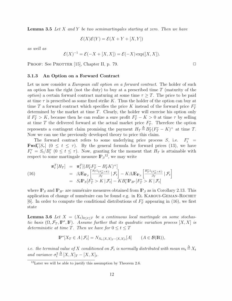
3.1.3 An Option on a Forward Contract

Let us now consider a European call option on a forward contract. The holder of suchan option has the right (not the duty) to buy at a prescribed time T (maturity of theoption) a certain forward contract maturing at some time τ ≥ T . The price to be paidat time τ is prescribed as some fixed strike K. Thus the holder of the option can buy attime T a forward contract which specifies the price K instead of the forward price F τ

T

determined by the market at time T . Clearly, the holder will exercise his option onlyif F τ

T > K, because then he can realize a sure profit F τT − K > 0 at time τ by selling

at time T the delivered forward at the actual market price F τT . Therefore the option

represents a contingent claim promising the payment HT∆=Bτ

T (F τT − K)+ at time T .

Now we can use the previously developed theory to price this claim.The forward contract refers to some underlying price process S, i.e. F τ

t =Fwdτ

t [Sτ ] (0 ≤ t ≤ τ). By the general formula for forward prices (13), we haveF τt = St/B

τt (0 ≤ t ≤ τ). Now, granting for the moment that HT is attainable with

respect to some martingale measure IPβ12, we may write

πTt [HT ] = πT

t [(BτTF

τT −Bτ

TK)+]

= βtIEIPβ

[ST 1Fτ

T>K

βT| Ft

]−KβtIEIPβ

[Bτ

T 1FτT>K

βT| Ft

]= StIPS[F τ

T > K | Ft] −KBτt IPBτ [F τ

T > K | Ft]

(16)

where IPS and IPBτ are numeraire measures obtained from IPβ as in Corollary 2.13. Thisapplication of change of numeraire can be found e.g. in El Karoui-Geman-Rochet[6]. In order to compute the conditional distributions of F τ

T appearing in (16), we firststate

Lemma 3.6 Let X = (Xt)0≤t≤T be a continuous local martingale on some stochas-tic basis (Ω,FT , IP

∗, IF). Assume further that its quadratic variation process [X,X] isdeterministic at time T . Then we have for 0 ≤ t ≤ T

IP∗[XT ∈ A | Ft] = NXt,[X,X]T−[X,X]t [A] (A ∈ B(IR)),

i.e. the terminal value of X conditioned on Ft is normally distributed with mean mt∆=Xt

and variance σ2t

∆= [X,X]T − [X,X]t.

12Later we will be able to justify this assumption by Theorem 2.6.

12

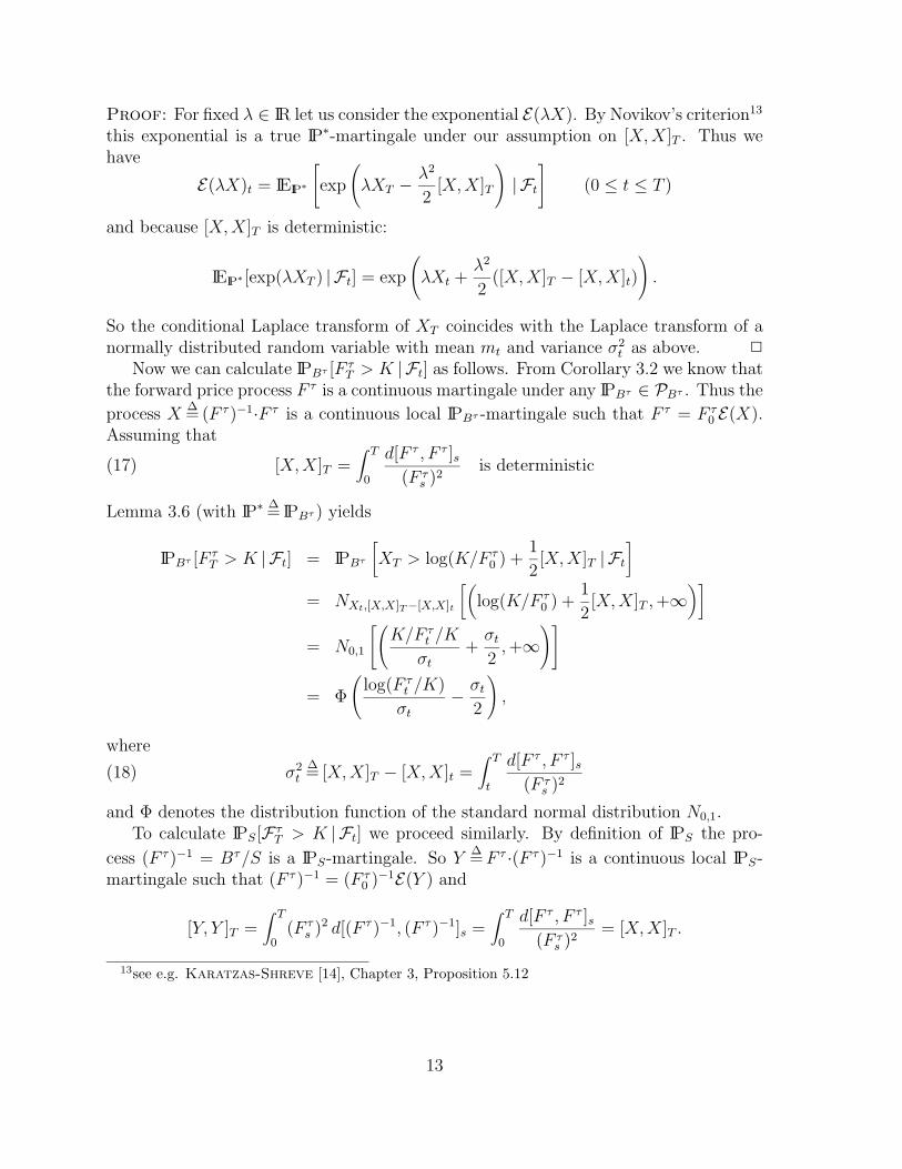
Proof: For fixed λ ∈ IR let us consider the exponential E(λX). By Novikov’s criterion13

this exponential is a true IP∗-martingale under our assumption on [X,X]T . Thus wehave

E(λX)t = IEIP∗

[exp

(λXT − λ2

2[X,X]T

)| Ft

](0 ≤ t ≤ T )

and because [X,X]T is deterministic:

IEIP∗ [exp(λXT ) | Ft] = exp

(λXt +

λ2

2([X,X]T − [X,X]t)

).

So the conditional Laplace transform of XT coincides with the Laplace transform of anormally distributed random variable with mean mt and variance σ2

t as above.

Now we can calculate IPBτ [F τT > K | Ft] as follows. From Corollary 3.2 we know that

the forward price process F τ is a continuous martingale under any IPBτ ∈ PBτ . Thus the

process X∆= (F τ )−1·F τ is a continuous local IPBτ -martingale such that F τ = F τ

0 E(X).Assuming that

[X,X]T =∫ T

0

d[F τ , F τ ]s(F τ

s )2is deterministic(17)

Lemma 3.6 (with IP∗ ∆= IPBτ ) yields

IPBτ [F τT > K | Ft] = IPBτ

[XT > log(K/F τ

0 ) +1

2[X,X]T | Ft

]

= NXt,[X,X]T−[X,X]t

[(log(K/F τ

0 ) +1

2[X,X]T ,+∞

)]

= N0,1

[(K/F τ

t /K

σt

+σt

2,+∞

)]

= Φ

(log(F τ

t /K)

σt

− σt

2

),

where

σ2t

∆= [X,X]T − [X,X]t =

∫ T

t

d[F τ , F τ ]s(F τ

s )2(18)

and Φ denotes the distribution function of the standard normal distribution N0,1.To calculate IPS[F τ

T > K | Ft] we proceed similarly. By definition of IPS the pro-

cess (F τ )−1 = Bτ/S is a IPS-martingale. So Y∆=F τ ·(F τ )−1 is a continuous local IPS-

martingale such that (F τ )−1 = (F τ0 )−1E(Y ) and

[Y, Y ]T =∫ T

0(F τ

s )2 d[(F τ )−1, (F τ )−1]s =∫ T

0

d[F τ , F τ ]s(F τ

s )2= [X,X]T .

13see e.g. Karatzas-Shreve [14], Chapter 3, Proposition 5.12

13

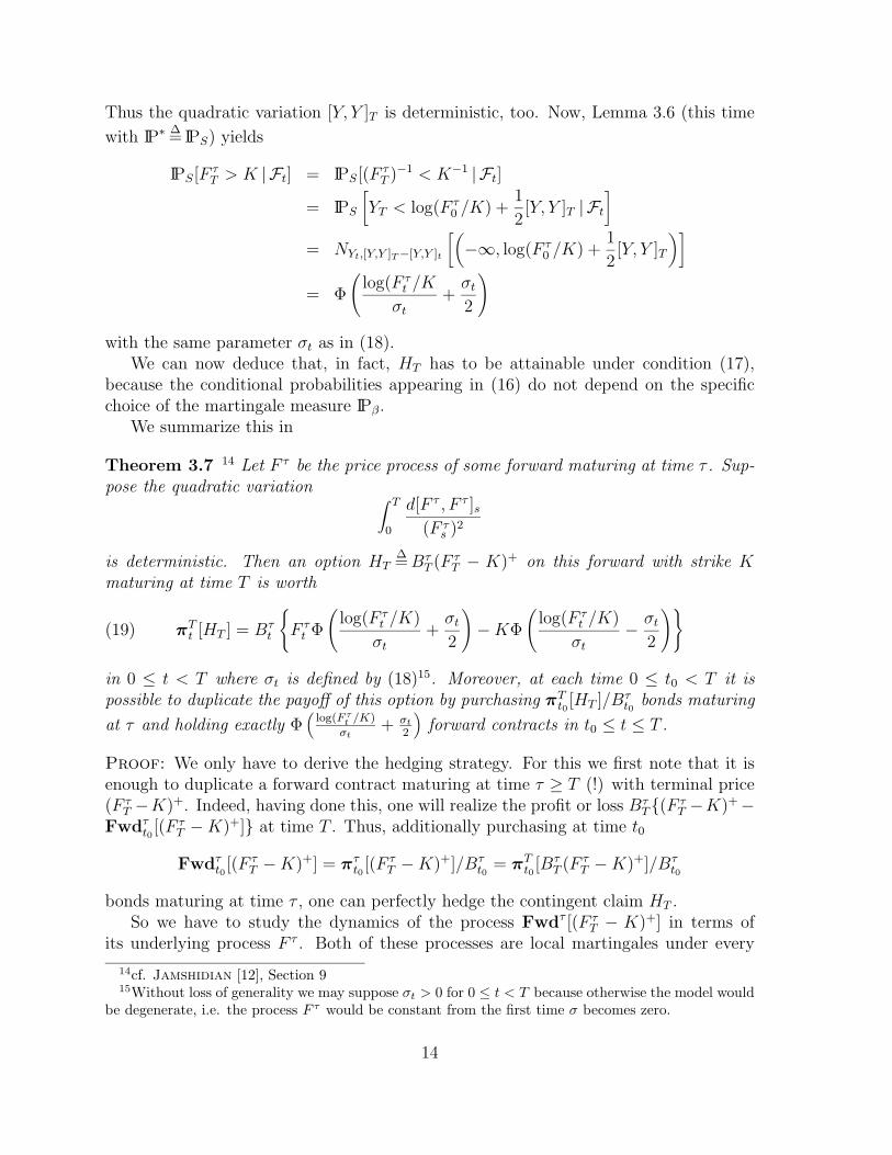
Thus the quadratic variation [Y, Y ]T is deterministic, too. Now, Lemma 3.6 (this time

with IP∗ ∆= IPS) yields

IPS[F τT > K | Ft] = IPS[(F τ

T )−1 < K−1 | Ft]

= IPS

[YT < log(F τ

0 /K) +1

2[Y, Y ]T | Ft

]

= NYt,[Y,Y ]T−[Y,Y ]t

[(−∞, log(F τ

0 /K) +1

2[Y, Y ]T

)]

= Φ

(log(F τ

t /K

σt

+σt

2

)

with the same parameter σt as in (18).We can now deduce that, in fact, HT has to be attainable under condition (17),

because the conditional probabilities appearing in (16) do not depend on the specificchoice of the martingale measure IPβ.

We summarize this in

Theorem 3.7 14 Let F τ be the price process of some forward maturing at time τ . Sup-pose the quadratic variation ∫ T

0

d[F τ , F τ ]s(F τ

s )2

is deterministic. Then an option HT∆=Bτ

T (F τT − K)+ on this forward with strike K

maturing at time T is worth

πTt [HT ] = Bτ

t

F τt Φ

(log(F τ

t /K)

σt

+σt

2

)−KΦ

(log(F τ

t /K)

σt

− σt

2

)(19)

in 0 ≤ t < T where σt is defined by (18)15. Moreover, at each time 0 ≤ t0 < T it ispossible to duplicate the payoff of this option by purchasing πT

t0[HT ]/Bτ

t0bonds maturing

at τ and holding exactly Φ(

log(F τt /K)

σt+ σt

2

)forward contracts in t0 ≤ t ≤ T .

Proof: We only have to derive the hedging strategy. For this we first note that it isenough to duplicate a forward contract maturing at time τ ≥ T (!) with terminal price(F τ

T −K)+. Indeed, having done this, one will realize the profit or loss BτT(F τ

T −K)+−Fwdτ

t0[(F τ

T −K)+] at time T . Thus, additionally purchasing at time t0

Fwdτt0[(F τ

T −K)+] = πτt0[(F τ

T −K)+]/Bτt0

= πTt0[Bτ

T (F τT −K)+]/Bτ

t0

bonds maturing at time τ , one can perfectly hedge the contingent claim HT .So we have to study the dynamics of the process Fwdτ [(F τ

T − K)+] in terms ofits underlying process F τ . Both of these processes are local martingales under every

14cf. Jamshidian [12], Section 915Without loss of generality we may suppose σt > 0 for 0 ≤ t < T because otherwise the model would

be degenerate, i.e. the process F τ would be constant from the first time σ becomes zero.

14

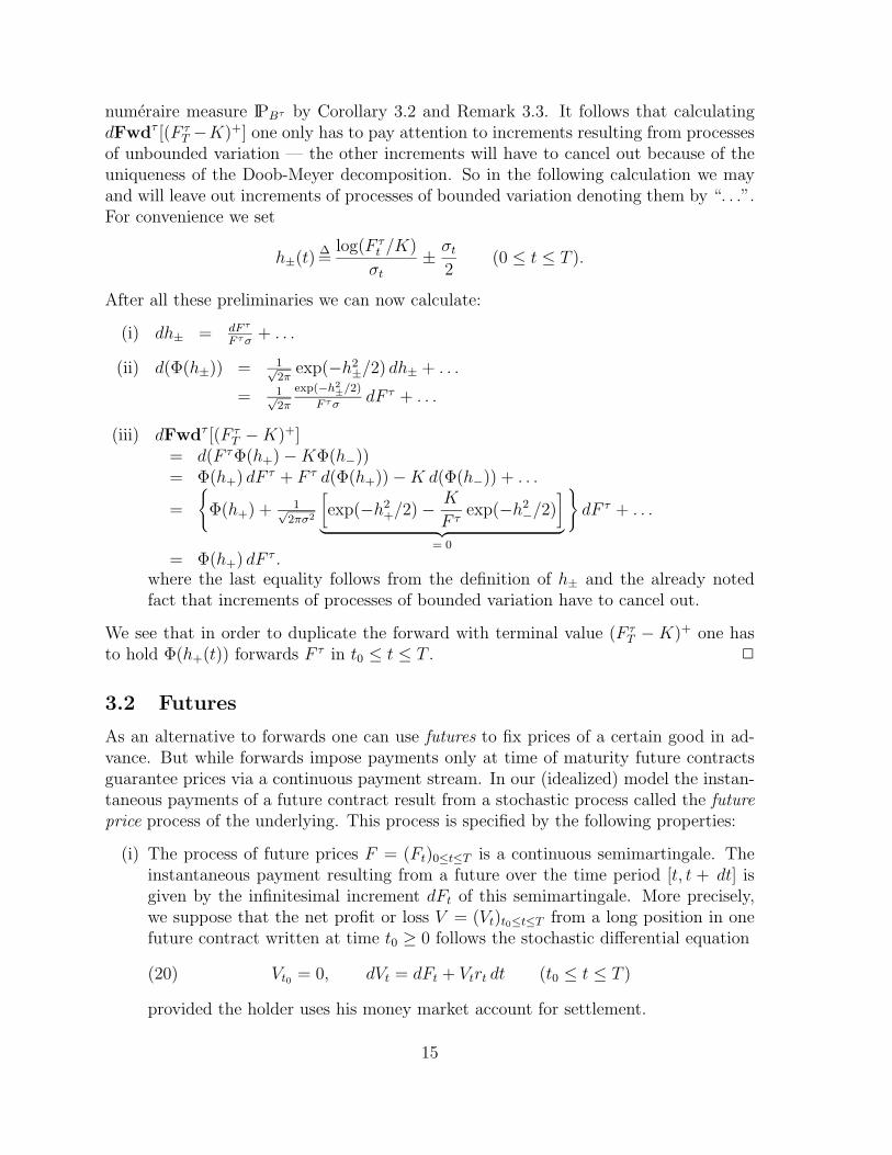
numeraire measure IPBτ by Corollary 3.2 and Remark 3.3. It follows that calculatingdFwdτ [(F τ

T −K)+] one only has to pay attention to increments resulting from processesof unbounded variation — the other increments will have to cancel out because of theuniqueness of the Doob-Meyer decomposition. So in the following calculation we mayand will leave out increments of processes of bounded variation denoting them by “. . .”.For convenience we set

h±(t)∆=

log(F τt /K)

σt

± σt

2(0 ≤ t ≤ T ).

After all these preliminaries we can now calculate:

(i) dh± = dF τ

F τσ+ . . .

(ii) d(Φ(h±)) = 1√2π

exp(−h2±/2) dh± + . . .

= 1√2π

exp(−h2±/2)

F τσdF τ + . . .

(iii) dFwdτ [(F τT −K)+]

= d(F τΦ(h+) −KΦ(h−))= Φ(h+) dF τ + F τ d(Φ(h+)) −K d(Φ(h−)) + . . .

=

Φ(h+) + 1√

2πσ2

[exp(−h2

+/2) − K

F τexp(−h2

−/2)]

︸ ︷︷ ︸= 0

dF τ + . . .

= Φ(h+) dF τ .where the last equality follows from the definition of h± and the already notedfact that increments of processes of bounded variation have to cancel out.

We see that in order to duplicate the forward with terminal value (F τT −K)+ one has

to hold Φ(h+(t)) forwards F τ in t0 ≤ t ≤ T .

3.2 Futures

As an alternative to forwards one can use futures to fix prices of a certain good in ad-vance. But while forwards impose payments only at time of maturity future contractsguarantee prices via a continuous payment stream. In our (idealized) model the instan-taneous payments of a future contract result from a stochastic process called the futureprice process of the underlying. This process is specified by the following properties:

(i) The process of future prices F = (Ft)0≤t≤T is a continuous semimartingale. Theinstantaneous payment resulting from a future over the time period [t, t + dt] isgiven by the infinitesimal increment dFt of this semimartingale. More precisely,we suppose that the net profit or loss V = (Vt)t0≤t≤T from a long position in onefuture contract written at time t0 ≥ 0 follows the stochastic differential equation

Vt0 = 0, dVt = dFt + Vtrt dt (t0 ≤ t ≤ T )(20)

provided the holder uses his money market account for settlement.

15

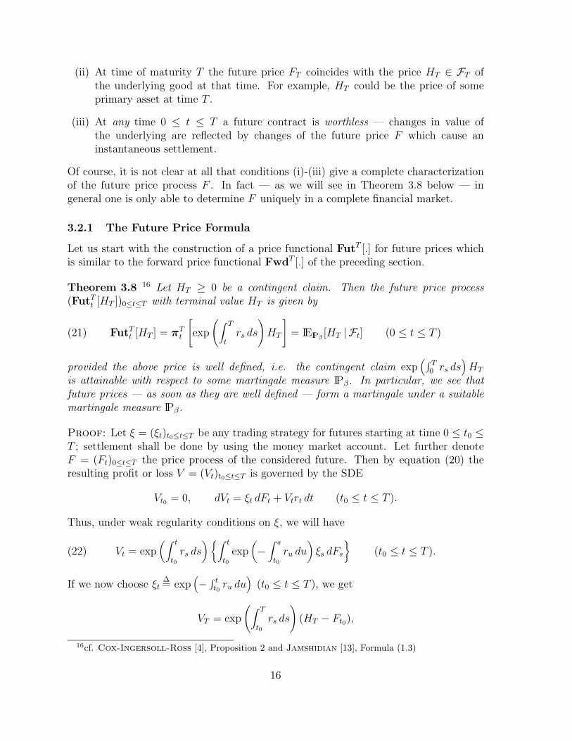
(ii) At time of maturity T the future price FT coincides with the price HT ∈ FT ofthe underlying good at that time. For example, HT could be the price of someprimary asset at time T .

(iii) At any time 0 ≤ t ≤ T a future contract is worthless — changes in value ofthe underlying are reflected by changes of the future price F which cause aninstantaneous settlement.

Of course, it is not clear at all that conditions (i)-(iii) give a complete characterizationof the future price process F . In fact — as we will see in Theorem 3.8 below — ingeneral one is only able to determine F uniquely in a complete financial market.

3.2.1 The Future Price Formula

Let us start with the construction of a price functional FutT [.] for future prices whichis similar to the forward price functional FwdT [.] of the preceding section.

Theorem 3.8 16 Let HT ≥ 0 be a contingent claim. Then the future price process(FutTt [HT ])0≤t≤T with terminal value HT is given by

FutTt [HT ] = πTt

[exp

(∫ T

trs ds

)HT

]= IEIPβ

[HT | Ft] (0 ≤ t ≤ T )(21)

provided the above price is well defined, i.e. the contingent claim exp(∫ T

0 rs ds)HT

is attainable with respect to some martingale measure IPβ. In particular, we see thatfuture prices — as soon as they are well defined — form a martingale under a suitablemartingale measure IPβ.

Proof: Let ξ = (ξt)t0≤t≤T be any trading strategy for futures starting at time 0 ≤ t0 ≤T ; settlement shall be done by using the money market account. Let further denoteF = (Ft)0≤t≤T the price process of the considered future. Then by equation (20) theresulting profit or loss V = (Vt)t0≤t≤T is governed by the SDE

Vt0 = 0, dVt = ξt dFt + Vtrt dt (t0 ≤ t ≤ T ).

Thus, under weak regularity conditions on ξ, we will have

Vt = exp(∫ t

t0rs ds

) ∫ t

t0exp

(−

∫ s

t0ru du

)ξs dFs

(t0 ≤ t ≤ T ).(22)

If we now choose ξt∆= exp

(− ∫ t

t0ru du

)(t0 ≤ t ≤ T ), we get

VT = exp

(∫ T

t0rs ds

)(HT − Ft0),

16cf. Cox-Ingersoll-Ross [4], Proposition 2 and Jamshidian [13], Formula (1.3)

16

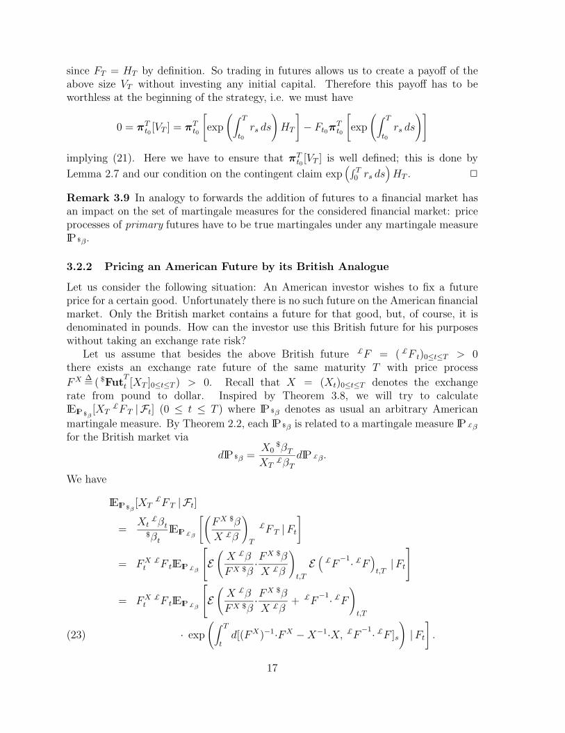
since FT = HT by definition. So trading in futures allows us to create a payoff of theabove size VT without investing any initial capital. Therefore this payoff has to beworthless at the beginning of the strategy, i.e. we must have

0 = πTt0[VT ] = πT

t0

[exp

(∫ T

t0rs ds

)HT

]− Ft0π

Tt0

[exp

(∫ T

t0rs ds

)]

implying (21). Here we have to ensure that πTt0[VT ] is well defined; this is done by

Lemma 2.7 and our condition on the contingent claim exp(∫ T

0 rs ds)HT .

Remark 3.9 In analogy to forwards the addition of futures to a financial market hasan impact on the set of martingale measures for the considered financial market: priceprocesses of primary futures have to be true martingales under any martingale measureIP $β.

3.2.2 Pricing an American Future by its British Analogue

Let us consider the following situation: An American investor wishes to fix a futureprice for a certain good. Unfortunately there is no such future on the American financialmarket. Only the British market contains a future for that good, but, of course, it isdenominated in pounds. How can the investor use this British future for his purposeswithout taking an exchange rate risk?

Let us assume that besides the above British future £F = ( £F t)0≤t≤T > 0there exists an exchange rate future of the same maturity T with price process

FX ∆= ( $Fut

T

t [XT ]0≤t≤T ) > 0. Recall that X = (Xt)0≤t≤T denotes the exchangerate from pound to dollar. Inspired by Theorem 3.8, we will try to calculateIEIP $β

[XT£F T | Ft] (0 ≤ t ≤ T ) where IP $β denotes as usual an arbitrary American

martingale measure. By Theorem 2.2, each IP $β is related to a martingale measure IP£β

for the British market via

dIP $β =X0

$βT

XT£βT

dIP£β.

We have

IEIP $β[XT

£F T | Ft]

=Xt

£βt

$βt

IEIP£β

[(FX $β

X £β

)T

£F T |Ft

]

= FXt

£F tIEIP£β

E

(X £β

FX $β·F

X $β

X £β

)t,T

E(

£F−1· £F

)t,T

|Ft

= FXt

£F tIEIP£β

E

(X £β

FX $β·F

X $β

X £β+ £F

−1· £F)t,T

· exp

(∫ T

td[(FX)−1·FX −X−1·X, £F

−1· £F ]s

)|Ft

].(23)

17

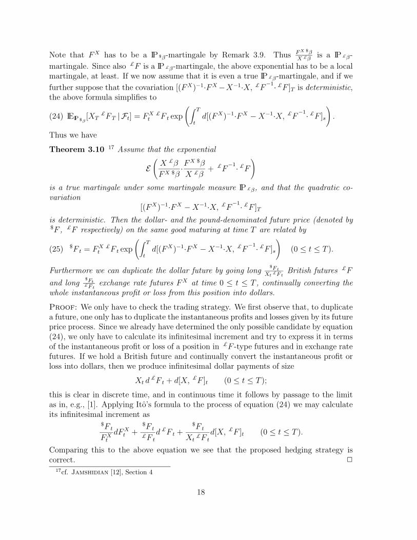
Note that FX has to be a IP $β-martingale by Remark 3.9. Thus FX $βX £β

is a IP£β-

martingale. Since also £F is a IP£β-martingale, the above exponential has to be a localmartingale, at least. If we now assume that it is even a true IP£β-martingale, and if we

further suppose that the covariation [(FX)−1·FX −X−1·X, £F−1· £F ]T is deterministic,

the above formula simplifies to

IEIP $β[XT

£F T | Ft] = FXt

£F t exp

(∫ T

td[(FX)−1·FX −X−1·X, £F

−1· £F ]s

).(24)

Thus we have

Theorem 3.10 17 Assume that the exponential

E(X £β

FX $β·F

X $β

X £β+ £F

−1· £F)

is a true martingale under some martingale measure IP£β, and that the quadratic co-variation

[(FX)−1·FX −X−1·X, £F−1· £F ]T

is deterministic. Then the dollar- and the pound-denominated future price (denoted by$F , £F respectively) on the same good maturing at time T are related by

$F t = FXt

£F t exp

(∫ T

td[(FX)−1·FX −X−1·X, £F

−1· £F ]s

)(0 ≤ t ≤ T ).(25)

Furthermore we can duplicate the dollar future by going long$F t

Xt£F t

British futures £F

and long$Ft£F t

exchange rate futures FX at time 0 ≤ t ≤ T , continually converting thewhole instantaneous profit or loss from this position into dollars.

Proof: We only have to check the trading strategy. We first observe that, to duplicatea future, one only has to duplicate the instantaneous profits and losses given by its futureprice process. Since we already have determined the only possible candidate by equation(24), we only have to calculate its infinitesimal increment and try to express it in termsof the instantaneous profit or loss of a position in £F -type futures and in exchange ratefutures. If we hold a British future and continually convert the instantaneous profit orloss into dollars, then we produce infinitesimal dollar payments of size

Xt d£F t + d[X, £F ]t (0 ≤ t ≤ T );

this is clear in discrete time, and in continuous time it follows by passage to the limitas in, e.g., [1]. Applying Ito’s formula to the process of equation (24) we may calculateits infinitesimal increment as

$F t

FXt

dFXt +

$F t

£F t

d £F t +$F t

Xt£F t

d[X, £F ]t (0 ≤ t ≤ T ).

Comparing this to the above equation we see that the proposed hedging strategy iscorrect.

17cf. Jamshidian [12], Section 4

18

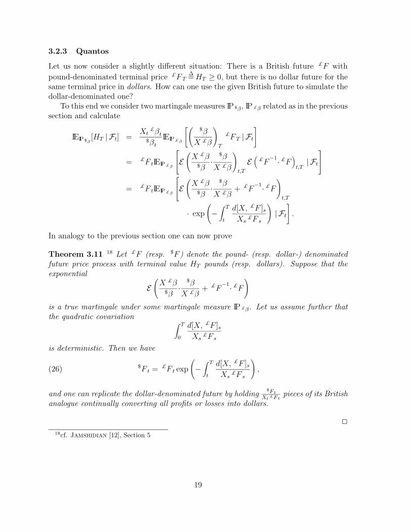
3.2.3 Quantos

Let us now consider a slightly different situation: There is a British future £F with

pound-denominated terminal price £F T∆=HT ≥ 0, but there is no dollar future for the

same terminal price in dollars. How can one use the given British future to simulate thedollar-denominated one?

To this end we consider two martingale measures IP $β, IP£β related as in the previoussection and calculate

IEIP $β[HT | Ft] =

Xt£βt

$βt

IEIP£β

[($β

X £β

)T

£F T | Ft

]

= £F tIEIP£β

E

(X £β

$β·

$β

X £β

)t,T

E(

£F−1· £F

)t,T

| Ft

= £F tIEIP£β

E

(X £β

$β·

$β

X £β+ £F

−1· £F)t,T

· exp

(−

∫ T

t

d[X, £F ]sXs

£F s

)| Ft

].

In analogy to the previous section one can now prove

Theorem 3.11 18 Let £F (resp. $F ) denote the pound- (resp. dollar-) denominatedfuture price process with terminal value HT pounds (resp. dollars). Suppose that theexponential

E(X £β

$β·

$β

X £β+ £F

−1· £F)

is a true martingale under some martingale measure IP£β. Let us assume further thatthe quadratic covariation ∫ T

0

d[X, £F ]sXs

£F s

is deterministic. Then we have

$F t = £F t exp

(−

∫ T

t

d[X, £F ]sXs

£F s

),(26)

and one can replicate the dollar-denominated future by holding$F t

Xt£F t

pieces of its Britishanalogue continually converting all profits or losses into dollars.

18cf. Jamshidian [12], Section 5

19

3.3 Swaps

As a last example from Jamshidian [12] we are going to derive a valuation formulaand a hedging strategy for continuous differential swaps. A differential swap expiringat time T , say, between the British and the U.S. financial market, promises its holderan infinitesimal dollar payment stream ( £rt − $rt) dt (0 ≤ t ≤ T ). More precisely: Ifan investor enters a differential swap at time t0 his cumulative return (Vt0,t)t0≤t≤T fromthis investment will develop satisfying

Vt0,t0 = 0, dVt0,t = Vt0,t$rt dt + ( £rt − $rt) dt (t0 ≤ t ≤ T )(27)

provided he reinvests his funds in the U.S. money market. So at time 0 ≤ t ≤ T he willhave earned the amount

Vt0,t = exp(∫ t

t0

$ru du) ∫ t

t0exp

(−

∫ s

t0

$ru du)

( £rs − $rs) ds.(28)

Thus, the value of the above continuous differential swap has to coincide with the valueof a payment of size Vt0,T at time T . Therefore it is enough to price and hedge thiscontingent claim. For this we first recall some well-known results on the relation betweeninterest rates and bonds.

3.3.1 Forward Rates and Bonds

Forward rates allow an investor to fix his interest rates in advance. This is done asfollows: At time t he agrees to invest a certain amount of his wealth over an infinitesimalfuture time period [s, s+ ds] at interest rate rst ∈ Ft which is fixed at time t. Whateverthe true interest rate might be at time s, he will have the interest return rst ds on hisinvestment. The forward rate rst is determined so that — in analogy with the classicalforward contracts — the above agreement itself does not cost anything.

We assume that besides the “usual” stocks and bonds one can trade forward ratesfor every future date 0 ≤ s ≤ T at any time 0 ≤ t ≤ s. Since both bonds and forwardrates allow to fix future interest rates — although in different ways — there has tobe some relation between them. Under weak regularity conditions this is given by thewell-known formulae

Bst = exp

(−

∫ s

trut du

)IP-a.s., resp. rst = − 1

Bst

∂

∂sBs

t IP ⊗ ds-a.e.(29)

So far we have always argued in terms of a given finite number of assets. From now onwe will consider the full continuum Bs (0 ≤ s ≤ T ) of bond price processes. From amathematical point of view, this causes many technical problems whose solution lies farbeyond the scope of this paper. For instance, we do not try to reduce the existence of anequivalent martingale measure to the absence of arbitrage as in Theorem 2.1. Insteadwe simply introduce the

Assumption 3.12 There is at least one equivalent martingale measure for all stocksand the whole continuum of bonds.

20

Under this standing assumption we have the well-known

Theorem 3.13 19 At time t ≥ 0 forward rates rst (t ≤ s ≤ T ) satisfy

rst = IEIPBs [rs | Ft] (t ≤ s ≤ T ) IP ⊗ ds-a.e.(30)

for IPBs ∈ PBs. In particular, for a.e. fixed maturity 0 ≤ s ≤ T the forward rates(rst )0≤t≤s form a IPBs-martingale.

Proof: First we note that for any martingale measure IPβ and 0 ≤ t ≤ s ≤ T we have

Bst = IEIPβ

[exp

(−

∫ s

tru du

)| Ft

]

= IEIPβ

[1 +

∫ s

t

∂

∂τ

exp

(−

∫ τ

tru du

)dτ | Ft

]

= 1 −∫ s

tIEIPβ

[exp

(−

∫ τ

tru du

)rτ | Ft

]dτ

= 1 −∫ s

tBτ

t IEIPBτ [rτ | Ft] dτ

Now comparing this to

Bst = exp

(−

∫ s

trut du

)

= 1 +∫ s

t

∂

∂τ

exp

(−

∫ τ

trut du

)dτ

= 1 −∫ s

tBτ

t rτt dτ

yields (30).

Remark 3.14 By the above theorem, we may interpret the forward rates rst (0 ≤ t ≤ s)as unbiased estimators for rs under any numeraire measure IPBs . For this reason theabove equality is often called “unbiased expectation hypothesis”.

In order to analyze the dynamics of bonds and forward rates we introduce the fol-lowing Heath-Jarrow-Morton [9]-type assumption:

Assumption 3.15 There is a finite number I of continuous semimartingales M i (i =1, . . . , I) such that for suitable bounded20, B([0, T ]) ⊗ P-measurable H i = (Hs,i

t ; 0 ≤s, t ≤ T ) (i = 1, . . . , I) the dynamics of forward rates are given by

rst = rs0 +∑i

∫ t

0Hs,i

u dM iu (0 ≤ t ≤ s).(31)

19cf. e.g. Ingersoll [10], Chapter 1820Of course, the boundedness-assumption is introduced only for convenience and can be relaxed

considerably.

21

The dynamics of forward rates translates into the dynamics of bonds as follows:

Proposition 3.16 Under Assumption 3.15 bond prices are governed by the SDE

dBst

Bst

= rt dt−∑

i

(∫ st H

v,it dv

)dM i

t

+ 12

∑i,j

(∫ st H

v,it dv

) (∫ st H

v,jt dv

)d[M i,M j]t.

(32)

Proof: First (29) implies

dBst = −Bs

t d(∫ s

.rv. dv

)t+

1

2Bs

t d[∫ s

.rv. dv,

∫ s

.rv. dv]t.

By Lemma 3.17 below, we may calculate the above stochastic differentials as

d(∫ s

.rv. dv

)t= −rtt dt +

∑i

(∫ s

tHv,i

t dv)dM i

t

and

d[∫ s

.rv. dv,

∫ s

.rv. dv]t =

∑i,j

(∫ s

tHv,i

t dv) (∫ s

tHv,j

t dv)d[M i,M j]t.

Employing these equations in the first one yields the result.

The Fubini-type argument in the preceding proof will be used again in the sequel,and so we state it explicitly:

Lemma 3.17 Let Y = (Yt)0≤t≤s be a process of the form

Yt =∫ s

tZv

t dv (0 ≤ t ≤ s)

where Zv = (Zvt )0≤t≤v; 0 ≤ v ≤ s is a family of semimartingales satisfying

Zvt = Zv

0 +∫ t

0Hv

u dMu (0 ≤ t, v ≤ s)

for some continuous semimartingale M and some bounded B([0, T ]) ⊗ P-measurableHv

t = H(v, t, ω). Then the dynamics of Y can be read off

Yt =∫ s

0Zv

0 dv −∫ t

0Zu

u du +∫ t

0

(∫ s

uHv

u dv)dMu (0 ≤ t ≤ s).(33)

Proof: Let λ denote the Lebesgue measure restricted on (0, s). We may write

Yt =∫

1[0,v)(t)Zvt λ(dv) (0 ≤ t ≤ s).

20P denotes the σ-algebra of IF-predictable sets.

22

Applying Ito’s formula to the integrand yields

1[0,v)(t)Zvt = 1[0,v)(0)Zv

0 +∫ t

0Zv

u− d1[0,v)(u) +∫ t

01[0,v](u) dZv

u

= Zv0 − Zv

v1[0,t](v) +∫ t

01[0,v](u) dZv

u

Employing this in the first equation and using Theorem 46 in Chapter IV of Protter[15] we have

Yt =∫

Zv0 λ(dv) −

∫Zv

v1[0,t](v)λ(dv)(34)

+∫ (∫ t

01[0,v](u)Hv

u dMu

)λ(dv)

=∫

Zv0 λ(dv) −

∫Zv

v1[0,t](v)λ(dv)

+∫ t

0

(∫1[0,v](u)Hv

u λ(dv))dMu

=∫ s

0Zv

0 dv −∫ t

0Zu

u du +∫ t

0

(∫ s

uHv

u dv)dMu

for 0 ≤ t ≤ s.

3.3.2 Pricing Continuous Differential Swaps

After these preliminaries let us now price the contingent claim Vt0,T given by equation(28). By Assumption 3.12 we have a martingale measure IP $β for the whole (U.S.-)market including the continuum of American and (converted) British bonds.

Of course, we want to calculate

IP $βπT

t [Vt0,T ] = $βtIEIP $β

[Vt0,T

$βT

| Ft

]

= IEIP $β

[exp

(−

∫ T

t

$ru du

)Vt0,T | Ft

]

= Vt0,t +∫ T

tIEIP $β

[exp

(−

∫ s

t

$ru du)

( £rs − $rs) | Ft

]ds

= Vt0,t +∫ T

t

$Bs

t IEIP $Bs [

£rs − $rs | Ft] ds

= Vt0,t +∫ T

t

$Bs

t

(IEIP $B

s [£rs | Ft] − $r

s

t

)ds

explicitly. For the last but one equality we performed a change of numeraire from $βto $B

sas in Theorem 2.10. For the last equality we used the unbiased expectation

hypothesis for $rs under IP $Bs (cf. Lemma 3.13).

So the only problem to solve is the calculation of IEIP $Bs [ £rs | Ft] (0 ≤ t ≤ s ≤ T ).

This will be done using the unbiased expectation hypothesis for the British market. We

23

note that, in analogy to Theorem 2.2, from IP $Bs we get a numeraire measure IP£Bs for

the British market by

dIP $Bs

dIP£Bs| Ft

∆=

X0$B

s

t

Xt£Bs

t

= X0(Fst )−1 (0 ≤ t ≤ s ≤ T ).(35)

Here F s ∆= (X £B

s)/ $B

sis obviously a IP $B

s-martingale (so its inverse becomes a IP£Bs-martingale) which may be interpreted as forward exchange rate from pound to dollarwith maturity s. Thus

IEIP $Bs [

£rs | Ft] = F st IEIP£B

s

[£rs(F

ss )−1 | Ft

]= IEIP£B

s

[£r

s

sE(F s·(F s)−1

)t,s

| Ft

].

The exponential is a local martingale with respect to IP£Bs . If we assume that it is atrue martingale, then, noting that the same is true for £r

s(cf. Lemma 3.13), we get

IEIP $Bs [

£rs | Ft]

= IEIP£Bs

[(£r

s

t +∫ s

td( £r

s)u

) (1 +

∫ s

tdE

(F s·(F s)−1

)t,u

)| Ft

]

= £rs

t + IEIP£Bs

[(∫ s

td( £r

s)u

) (∫ s

tdE

(F s·(F s)−1

)t,u

)| Ft

]

= £rs

t + IEIP£Bs

[∫ s

tE

(F s·(F s)−1

)t,u

d[

£rs, F s·(F s)−1

]u| Ft

].

If we suppose that the quadratic covariation process

[£r

s, F s·(F s)−1

]u

= −∫ u

0

d[

£rs, F s

]v

F sv

(0 ≤ u ≤ s)

is deterministic, we may conclude by Fubini’s theorem

IEIP $Bs [

£rs | Ft] = £rs

t −∫ s

t

d[

£rs, F s

]u

F su

.

Finally, we get the following price process:

IP $βπT

t [Vt0,T ] = Vt0,t +

∫ T

t

$Bs

t

£r

s

t −∫ s

t

d[

£rs, F s

]u

F su

− $rs

t

ds

= Vt0,t +

∫ T

t

$Bs

t

£r

s

t −∫ s

t

d[

£rs, F s

]u

F su

ds

+ $B

T

t − 1,(36)

where for the second equality we used the definition of dollar-forward rates.

24

This implies the following IP $β-price process V = (Vt0)0≤t0≤T = (IP $βπT

t0[Vt0,T ])0≤t0≤T

for our continuous differential swap:

Vt0 =

∫ T

t0

$Bs

t0

£r

s

t0−

∫ s

t0

d[

£rs, F s

]u

F su

ds

+ $B

T

t0− 1 (0 ≤ t0 ≤ T ).(37)

We summarize these results in

Proposition 3.18 Let IP $β be a martingale measure for the whole financial market in-cluding the continuum of American and (converted) British bonds. From this martingalemeasure we get by Theorem 2.10 a numeraire measure IP $B

s for each American bond$B

s(0 ≤ s ≤ T ). From each measure IP $B

s we can construct a numeraire measureIP£Bs for the British market via formula (35).

Suppose for each 0 ≤ s ≤ T the exponential E (F s·(F s)−1) is a true IP $Bs-martingale

where F s ∆=X £B

s/ $B

s. Assume furthermore the quadratic covariation process

[£r

s, F s·(F s)−1

]u

= −∫ u

0

d[

£rs, F s

]v

F sv

(0 ≤ u ≤ s)

to be deterministic. Then we get the following IP $β-price process V = (Vt)0≤t≤T for ourcontinuous differential swap:

Vt =

∫ T

t

$Bs

t

£r

s

t −∫ s

t

d[

£rs, F s

]u

F su

ds

+ $B

T

t − 1 (0 ≤ t ≤ T ).(38)

3.3.3 Hedging Continuous Differential Swaps

Let us now derive a hedging strategy against the above continuous differential swap. Tohedge a differential swap sold at time t0 one should try to duplicate the payoff Vt0,T withmaturity T which is defined by equation (28); see the beginning of Section 3.3. Startingfrom formula (36) we will show below that the IP $β-price dynamics of this contingentclaim is given by

IP $βπT

t [Vt0,T ] = IP $βπT

t [Vt0,T ]

+∫ tt0

Vt0,u−1$βu

d $βu

+∫ tt0d( $B

T)u

+∫ Tt0

∫ tt0

1[0,s](u)( £rsu − csu) d(

$Bs)u

ds

− ∫ tt0

$BTu

Xu£BT

u

d(X £BT)u

− ∫ Tt0

∫ tt0

1[0,s](u)$r

su

$Bsu

Xu£Bs

ud(X £B

s)u

ds

(39)

25

provided forward rates satisfy Assumption 3.15. Here we set

cst∆=

∫ t

t0

d[ £rs, F s]u

F su

(t0 ≤ t ≤ s ≤ T ).

Recall that this covariation process is supposed to be deterministic.

Remark 3.19 In Section 2 we introduced the notion “portfolio strategy” for a financialmarket containing only a finite number of assets. In an infinite dimensional market,Bjork-Di Masi-Kabanov-Runggaldier [2] suggests to interpret a strategy in acontinuum of bonds as a predictable measure-valued process. Since we do not wish todiscuss the corresponding theory of stochastic integrals in more detail21, in the sequelwe will tacitly assume the occurring integrals to be well defined.

Equation (39) suggests to consider the following strategy:

• invest Vt0,t − 1 dollar in the U.S. money market;

• hold one American bond of maturity T ;

• be long ( £rst − cst) ds American bonds maturing at time s ∈ [t, T ];

• invest 1 dollar in the British money market account;

• go short$B

Tt

Xt£BT

t

British bonds of maturity T ;

• sell$r

st

$Bst

Xt£Bs

tds British zero-bonds maturing in s ∈ [t, T ].

In fact, this strategy is selffinancing and a perfect hedge for Vt0,T because on the onehand, by definition, it duplicates the changes in value of this contingent claim and onthe other hand it uses precisely the wealth available, as one can easily see from thefollowing table:

Position in ... ... has dollar value

American money market Vt0,t − 1

dollar-denominated bonds

· maturing at time T $BT

t

· maturing at time s ∈ [t, T ]∫ Tt ( £r

su − csu)

$Bs

u ds

British money market 1

pound-denominated bonds

· maturing at time T − $BT

u

· maturing at time s ∈ [t, T ] − ∫ Tt

$rs

u$B

s

u = $BT

u − 1

whole portfolio Vt0,t − 1 + $BT

t +∫ Tt ( £r

st − cst)

$Bs

t ds = IP $βπT

t [Vt0,T ]

21see [2] for a rigorous treatment of this question

26

Thus we have

Theorem 3.20 Under the assumptions of Proposition 3.18 and Assumption 3.15 onecan hedge a short position in a continuous differential swap using the above tradingstrategy.

Remark 3.21 Note that we only priced the considered swap with respect to some fixedmartingale measure IP $β. Now, the above hedging strategy yields an argument, why onemight want to view the right side of (37) as the only arbitrage free price for this contin-gent claim. Unfortunately, we have not introduced a concept of admissibility for strate-gies in a continuum of bonds that would guarantee the duplication argument to produceunique prices. Bjork-Di Masi-Kabanov-Runggaldier [2] define a measure-valuedstrategy to be admissible, if the resulting wealth process is nonnegative. Since the con-tingent claim Vt0,T might be negative, this definition, unfortunately, does not fit intoour context. So we would need a definition of admissibility which is similar to the onein Definition 2.4. But this would need an extension of Theorem 2.6 to the context of aninfinite financial market.

Let us now prove equation (39). This will be done using our Fubini-type Lemma 3.17and Proposition 3.16 on the relation between forward rate- and bond price-dynamics.First, applying Ito’s Lemma to the “ds”-integrand in formula (36) allows us to splitIP $βπ

T

t [Vt0,T ] into six summands:

IP $βπT

t [Vt0,T ] = Vt0,t + $BT

t − 1 (It)

+∫ Tt

$Bs

t0( £r

st0− cst0) ds (IIt)

+∫ Tt

∫ tt0( £r

su − csu) d(

$Bs)uds (IIIt)

+∫ Tt

∫ tt0

$Bs

ud(£r

s)u

ds (IVt)

− ∫ Tt

∫ tt0

$Bs

u d(cs)u

ds (Vt)

+∫ Tt

∫ tt0d[ $B

s, £r

s]u

ds (VIt).

Now we are going to determine one by one the dynamics of (It) - (VIt):

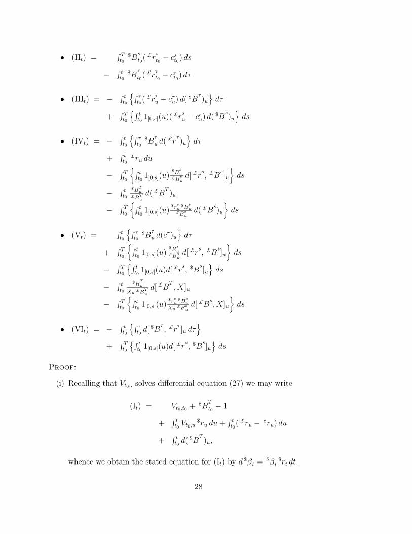
Lemma 3.22 Under Assumption 3.15 we have

• (It) = $BT

t0− 1

+∫ tt0

Vt0,u−1$βu

d $βu +∫ tt0

£ru du +∫ tt0d( $B

T)u

27

• (IIt) =∫ Tt0

$Bs

t0( £r

st0− cst0) ds

− ∫ tt0

$Bτ

t0( £r

τt0− cτt0) dτ

• (IIIt) = − ∫ tt0

∫ τt0( £r

τu − cτu) d(

$Bτ)u

dτ

+∫ Tt0

∫ tt0

1[0,s](u)( £rsu − csu) d(

$Bs)u

ds

• (IVt) = − ∫ tt0

∫ τt0

$Bτ

u d(£r

τ)u

dτ

+∫ tt0

£ru du

− ∫ Tt0

∫ tt0

1[0,s](u)$B

su

£Bsud[ £r

s, £B

s]u

ds

− ∫ tt0

$BTu

£BTu

d( £BT)u

− ∫ Tt0

∫ tt0

1[0,s](u)$r

su

$Bsu

£Bsu

d( £Bs)u

ds

• (Vt) =∫ tt0

∫ τt0

$Bτ

u d(cτ )u

dτ

+∫ Tt0

∫ tt0

1[0,s](u)$B

su

£Bsud[ £r

s, £B

s]u

ds

− ∫ Tt0

∫ tt0

1[0,s](u)d[ £rs, $B

s]u

ds

− ∫ tt0

$BTu

Xu£BT

u

d[ £BT, X]u

− ∫ Tt0

∫ tt0

1[0,s](u)$r

su

$Bsu

Xu£Bs

ud[ £B

s, X]u

ds

• (VIt) = − ∫ tt0

∫ τt0d[ $B

τ, £r

τ]u dτ

+

∫ Tt0

∫ tt0

1[0,s](u)d[ £rs, $B

s]u

ds

Proof:

(i) Recalling that Vt0,. solves differential equation (27) we may write

(It) = Vt0,t0 + $BT

t0− 1

+∫ tt0Vt0,u

$ru du +∫ tt0( £ru − $ru) du

+∫ tt0d( $B

T)u,

whence we obtain the stated equation for (It) by d $βt = $βt$rt dt.

28

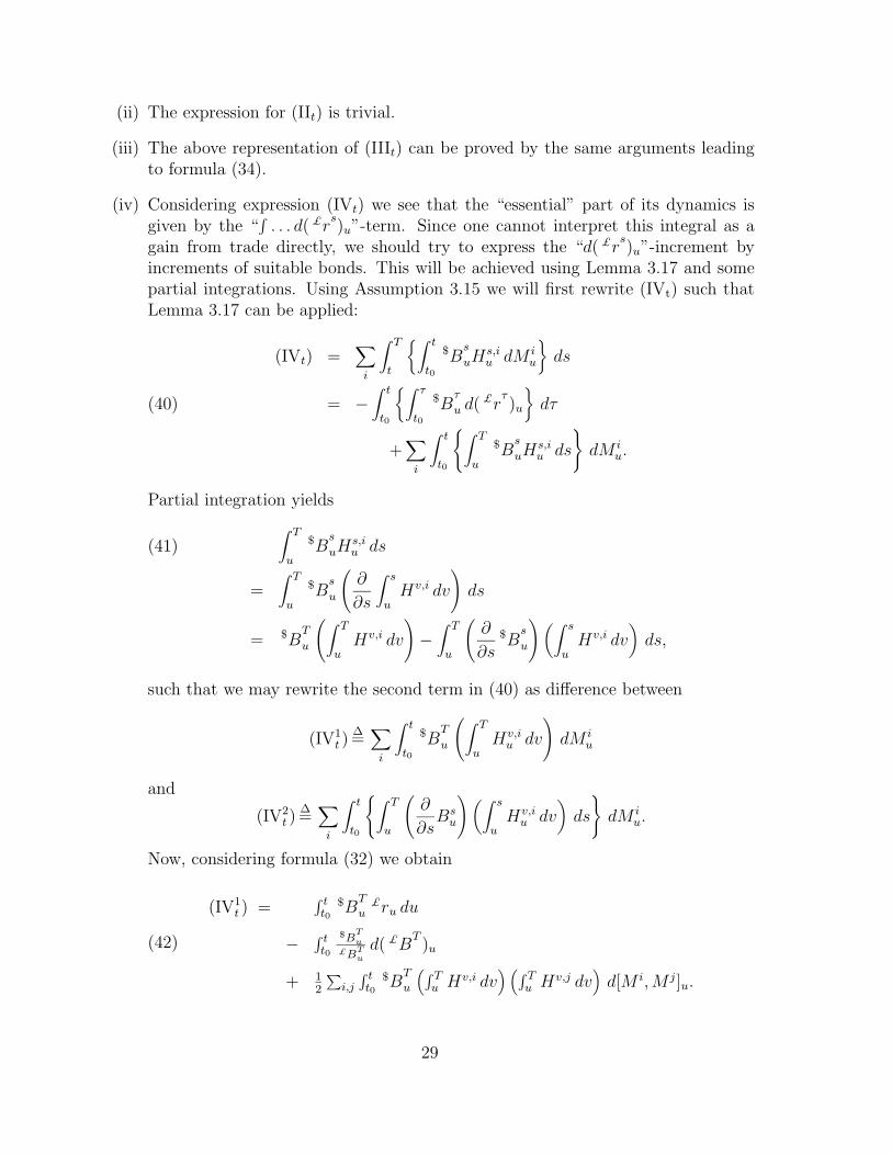
(ii) The expression for (IIt) is trivial.

(iii) The above representation of (IIIt) can be proved by the same arguments leadingto formula (34).

(iv) Considering expression (IVt) we see that the “essential” part of its dynamics isgiven by the “

∫. . . d( £r

s)u”-term. Since one cannot interpret this integral as a

gain from trade directly, we should try to express the “d( £rs)u”-increment by

increments of suitable bonds. This will be achieved using Lemma 3.17 and somepartial integrations. Using Assumption 3.15 we will first rewrite (IVt) such thatLemma 3.17 can be applied:

(IVt) =∑i

∫ T

t

∫ t

t0

$Bs

uHs,iu dM i

u

ds

= −∫ t

t0

∫ τ

t0

$Bτ

u d(£r

τ)u

dτ(40)

+∑i

∫ t

t0

∫ T

u

$Bs

uHs,iu ds

dM i

u.

Partial integration yields

∫ T

u

$Bs

uHs,iu ds(41)

=∫ T

u

$Bs

u

(∂

∂s

∫ s

uHv,i dv

)ds

= $BT

u

(∫ T

uHv,i dv

)−

∫ T

u

(∂

∂s$B

s

u

) (∫ s

uHv,i dv

)ds,

such that we may rewrite the second term in (40) as difference between

(IV1t )

∆=

∑i

∫ t

t0

$BT

u

(∫ T

uHv,i

u dv

)dM i

u

and

(IV2t )

∆=

∑i

∫ t

t0

∫ T

u

(∂

∂sBs

u

) (∫ s

uHv,i

u dv)ds

dM i

u.

Now, considering formula (32) we obtain

(IV1t ) =

∫ tt0

$BT

u£ru du

− ∫ tt0

$BTu

£BTu

d( £BT)u

+ 12

∑i,j

∫ tt0

$BT

u

(∫ Tu Hv,i dv

) (∫ Tu Hv,j dv

)d[M i,M j]u.

(42)

29

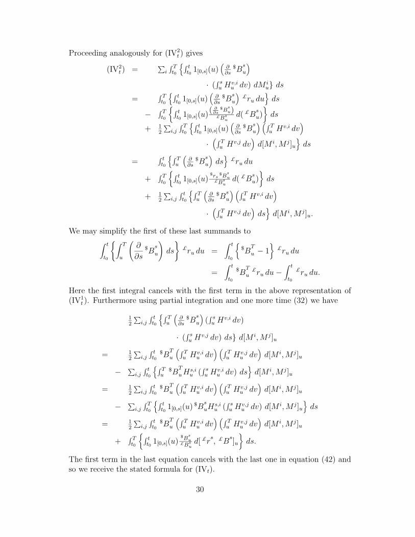
Proceeding analogously for (IV2t ) gives

(IV2t ) =

∑i

∫ Tt0

∫ tt0

1[0,s](u)(

∂∂s

$Bs

u

)· (

∫ su H

v,iu dv) dM i

u ds

=∫ Tt0

∫ tt0

1[0,s](u)(

∂∂s

$Bs

u

)£ru du

ds

− ∫ Tt0

∫ tt0

1[0,s](u)( ∂∂s

$Bsu)

£Bsu

d( £Bsu)

ds

+ 12

∑i,j

∫ Tt0

∫ tt0

1[0,s](u)(

∂∂s

$Bs

u

) (∫ Tu Hv,i dv

)·

(∫ Tu Hv,j dv

)d[M i,M j]u

ds

=∫ tt0

∫ Tu

(∂∂s

$Bs

u

)ds

£ru du

+∫ Tt0

∫ tt0

1[0,s](u)$rs $B

su

£Bsu

d( £Bsu)

ds

+ 12

∑i,j

∫ tt0

∫ Tu

(∂∂s

$Bs

u

) (∫ Tu Hv,i dv

)·

(∫ Tu Hv,j dv

)ds

d[M i,M j]u.

We may simplify the first of these last summands to∫ t

t0

∫ T

u

(∂

∂s$B

s

u

)ds

£ru du =

∫ t

t0

$B

T

u − 1

£ru du

=∫ t

t0

$BT

u£ru du−

∫ t

t0

£ru du.

Here the first integral cancels with the first term in the above representation of(IV1

t ). Furthermore using partial integration and one more time (32) we have

12

∑i,j

∫ tt0

∫ Tu

(∂∂s

$Bs

u

)(∫ su H

v,i dv)

· (∫ su H

v,j dv) ds d[M i,M j]u

= 12

∑i,j

∫ tt0

$BT

u

(∫ Tu Hv,i

u dv) (∫ T

u Hv,ju dv

)d[M i,M j]u

− ∑i,j

∫ tt0

∫ Tu

$BT

uHs,iu (

∫ su H

v,iu dv) ds

d[M i,M j]u

= 12

∑i,j

∫ tt0

$BT

u

(∫ Tu Hv,i

u dv) (∫ T

u Hv,ju dv

)d[M i,M j]u

− ∑i,j

∫ Tt0

∫ tt0

1[0,s](u) $Bs

uHs,iu (

∫ su H

v,ju dv) d[M i,M j]u

ds

= 12

∑i,j

∫ tt0

$BT

u

(∫ Tu Hv,i

u dv) (∫ T

u Hv,ju dv

)d[M i,M j]u

+∫ Tt0

∫ tt0

1[0,s](u)$B

su

£Bsud[ £r

s, £B

s]u

ds.

The first term in the last equation cancels with the last one in equation (42) andso we receive the stated formula for (IVt).

30

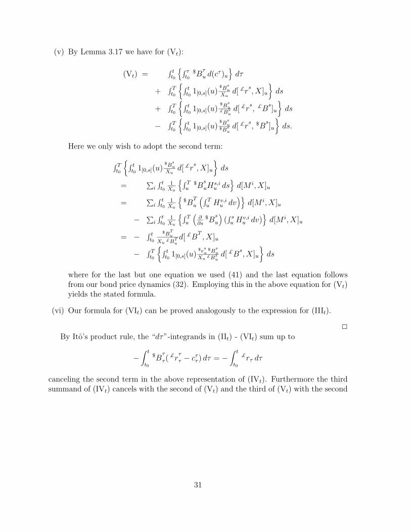
(v) By Lemma 3.17 we have for (Vt):

(Vt) =∫ tt0

∫ τt0

$Bτ

u d(cτ )u

dτ

+∫ Tt0

∫ tt0

1[0,s](u)$B

su

Xud[ £r

s, X]u

ds

+∫ Tt0

∫ tt0

1[0,s](u)$B

su

£Bsud[ £r

s, £B

s]u

ds

− ∫ Tt0

∫ tt0

1[0,s](u)$B

su

$Bsud[ £r

s, $B

s]u

ds.

Here we only wish to adopt the second term:

∫ Tt0

∫ tt0

1[0,s](u)$B

su

Xud[ £r

s, X]u

ds

=∑

i

∫ tt0

1Xu

∫ Tu

$Bs

uHs,iu ds

d[M i, X]u

=∑

i

∫ tt0

1Xu

$B

T

u

(∫ Tu Hv,i

u dv)

d[M i, X]u

− ∑i

∫ tt0

1Xu

∫ Tu

(∂∂s

$Bs

u

)(∫ su H

v,iu dv)

d[M i, X]u

= − ∫ tt0

$BTu

Xu£BT

u

d[ £BT, X]u

− ∫ Tt0

∫ tt0

1[0,s](u)$r

su

$Bsu

Xu£Bs

ud[ £B

s, X]u

ds

where for the last but one equation we used (41) and the last equation followsfrom our bond price dynamics (32). Employing this in the above equation for (Vt)yields the stated formula.

(vi) Our formula for (VIt) can be proved analogously to the expression for (IIIt).

By Ito’s product rule, the “dτ”-integrands in (IIt) - (VIt) sum up to

−∫ t

t0

$Bτ

τ (£r

τ

τ − cττ ) dτ = −∫ t

t0

£rτ dτ

canceling the second term in the above representation of (IVt). Furthermore the thirdsummand of (IVt) cancels with the second of (Vt) and the third of (Vt) with the second

31

of (VIt). Finally, we get

IP $βπT

t [Vt0,T ] = IP $βπT

t0[Vt0,T ]

+∫ tt0

Vt0,u−1$βu

d $βu

+∫ tt0

£ru du

+∫ tt0d( $B

T)u

+∫ Tt0

∫ tt0

1[0,s](u)( £rsu − csu) d(

$Bs)u

ds

− ∫ tt0

$BTu

£BTu

d( £BT)u

− ∫ tt0

$BTu

Xu£BT

u

d[ £BT, X]u

− ∫ Tt0

∫ tt0

1[0,s](u)$r

su

$Bsu

£Bsu

d( £Bs)u

ds

− ∫ Tt0

∫ tt0

1[0,s](u)$r

su

$Bsu

Xu£Bs

ud[ £B

s, X]u

ds.

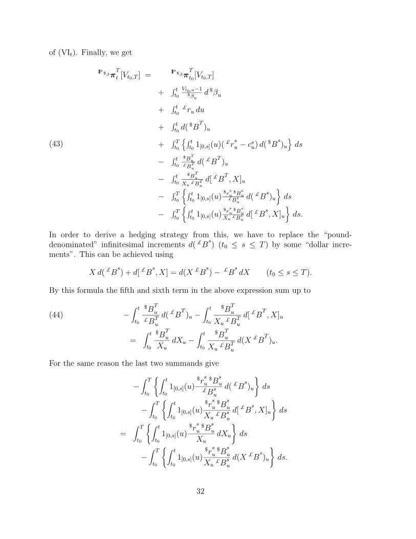
(43)

In order to derive a hedging strategy from this, we have to replace the “pound-denominated” infinitesimal increments d( £B

s) (t0 ≤ s ≤ T ) by some “dollar incre-

ments”. This can be achieved using

X d( £Bs) + d[ £B

s, X] = d(X £B

s) − £B

sdX (t0 ≤ s ≤ T ).

By this formula the fifth and sixth term in the above expression sum up to

−∫ t

t0

$BT

u

£BTu

d( £BT)u −

∫ t

t0

$BT

u

Xu£BT

u

d[ £BT, X]u(44)

=∫ t

t0

$BT

u

Xu

dXu −∫ t

t0

$BT

u

Xu£BT

u

d(X £BT)u.

For the same reason the last two summands give

−∫ T

t0

∫ t

t01[0,s](u)

$rs

u$B

s

u£Bs

u

d( £Bs)u

ds

−∫ T

t0

∫ t

t01[0,s](u)

$rs

u$B

s

u

Xu£Bs

u

d[ £Bs, X]u

ds

=∫ T

t0

∫ t

t01[0,s](u)

$rs

u$B

s

u

Xu

dXu

ds

−∫ T

t0

∫ t

t01[0,s](u)

$rs

u$B

s

u

Xu£Bs

u

d(X £Bs)u

ds.

32

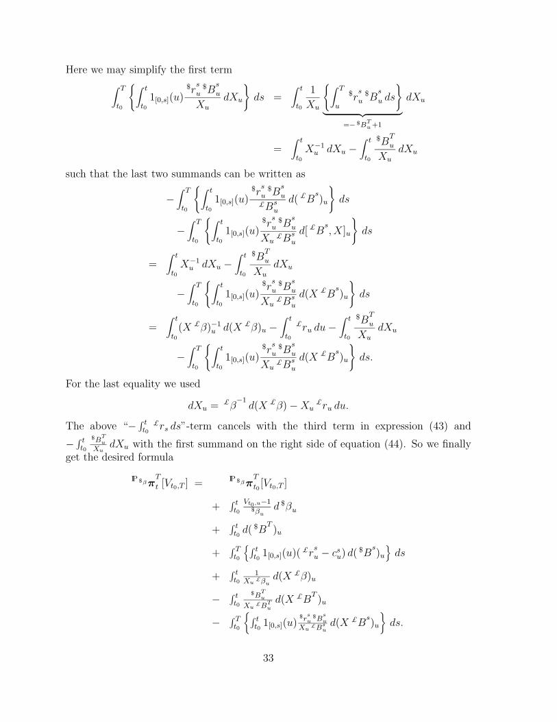
Here we may simplify the first term∫ T

t0

∫ t

t01[0,s](u)

$rs

u$B

s

u

Xu

dXu

ds =

∫ t

t0

1

Xu

∫ T

u

$rs

u$B

s

u ds

︸ ︷︷ ︸

=− $BTu+1

dXu

=∫ t

t0X−1

u dXu −∫ t

t0

$BT

u

Xu

dXu

such that the last two summands can be written as

−∫ T

t0

∫ t

t01[0,s](u)

$rs

u$B

s

u£Bs

u

d( £Bs)u

ds

−∫ T

t0

∫ t

t01[0,s](u)

$rs

u$B

s

u

Xu£Bs

u

d[ £Bs, X]u

ds

=∫ t

t0X−1

u dXu −∫ t

t0

$BT

u

Xu

dXu

−∫ T

t0

∫ t

t01[0,s](u)

$rs

u$B

s

u

Xu£Bs

u

d(X £Bs)u

ds

=∫ t

t0(X £β)−1

u d(X £β)u −∫ t

t0

£ru du−∫ t

t0

$BT

u

Xu

dXu

−∫ T

t0

∫ t

t01[0,s](u)

$rs

u$B

s

u

Xu£Bs

u

d(X £Bs)u

ds.

For the last equality we used

dXu = £β−1

d(X £β) −Xu£ru du.

The above “− ∫ tt0

£rs ds”-term cancels with the third term in expression (43) and

− ∫ tt0

$BTu

XudXu with the first summand on the right side of equation (44). So we finally

get the desired formula

IP $βπT

t [Vt0,T ] = IP $βπT

t0[Vt0,T ]

+∫ tt0

Vt0,u−1$βu

d $βu

+∫ tt0d( $B

T)u

+∫ Tt0

∫ tt0

1[0,s](u)( £rsu − csu) d(

$Bs)u

ds

+∫ tt0

1Xu

£βud(X £β)u

− ∫ tt0

$BTu

Xu£BT

u

d(X £BT)u

− ∫ Tt0

∫ tt0

1[0,s](u)$r

su

$Bsu

Xu£Bs

ud(X £B

s)u

ds.

33

References

[1] Bank, P. (1996): “Preisfunktionale und Hedging-Strategien fur Forwards, Futuresund Swaps in einem Semimartingalmodell”, Diplomarbeit, University of Bonn

[2] Bjork, T., G. Di Masi, Y. Kabanov, W. Runggaldier (1997): “Towards aGeneral Theory of Bond Markets”, Finance and Stochastics, 1, 141-174

[3] Black, F., M. Scholes (1973): “The Pricing of Options and Corporate Liabili-ties”, Journal of Political Economy, 81, 637-654

[4] Cox, J., J. E. Ingersoll, S. A. Ross (1981): “The Relation between ForwardPrices and Futures Prices”, Journal of Financial Economics, 9, 321-346

[5] Delbaen, F., W. Schachermeyer (1994): “A Gerneral Version of the Funda-mental Theorem of Asset Pricing”, Mathematische Annalen, 300, 463-520

[6] El Karoui, N., H. Geman, J.-C. Rochet (1994): “Changes of Numeraire,Changes of Probability Measure and Option Pricing”, Journal Applied Probability,32, 443-458

[7] Harrison, J. M., D. M. Kreps (1979): “Martingales and Arbitrage in Multi-period Securities Markets”, Journal of Economic Theory, 20, 381-408

[8] Harrison, J. M., R. Pliska (1981): “Martingales and Stochastic Integrals inthe Theory of Continuous Trading”, Stochastic Processes and their Applications,11, 215-260

[9] Heath, D., R. Jarrow, A. Morton (1992): “Bond Pricing and the TermStructure of Interest Rates: A New Methodology for Contingent Claims Valuation”,Econometrica, Vol. 60, No. 1, 77-105

[10] Ingersoll, J. (1987): “Theory of Financial Decision Making”, Totowa, N.J.:Rowman and Littlefield

[11] Jacka, S. D. (1992): “A Martingale Representation Result and an Applicationto Incomplete Financial Markets”, Mathematical Finance, Vol. 2, No. 4, 239-250

[12] Jamshidian, F. (1994): “Hedging quantos, differential swaps and ratios”, AppliedMathematical Finance, 1, 1-20

[13] Jamshidian, F. (1993): “Option and Futures Evaluation with DeterministicVolatilities”, Mathematical Finance, Vol. 3, No. 2, 149-159

[14] Karatzas, I., St. E. Shreve (1988): “Brownian Motion and Stochastic Calcu-lus”, Springer-Verlag, Berlin

[15] Protter, P. (1990): “Stochastic Integration and Differential Equations”,Springer-Verlag, Berlin

34