Pricing American-style Basket Options By Implied Binomial Tree Henry Wan * Draft: March 2002 Abstract It is known that the most difficult problem of pricing and hedging multi-asset basket options are those with both high dimensionality and early exercise. This article proposes a numerical algorithm by reducing multivariate distributions of a portfolio into a single variable and modeling that as a univariate stochastic process in the form of an implied binomial tree. It is demonstrated that the method provides a fast and flexible way of pricing and hedging high dimensional multi-asset basket options with early exercise. * This article is a report to the Applied Finance Project of University of California at Berkeley. The author is grateful for comments of traders at Wachovia Securities, Jens Jackwerth at University of Konstanz, Germany, and Mark Broadie at Columbia University. The author is particularly grateful for the extensive and insightful suggestions of Mark Rubinstein for advising the project.

Welcome message from author
This document is posted to help you gain knowledge. Please leave a comment to let me know what you think about it! Share it to your friends and learn new things together.
Transcript

Pricing American-style Basket Options By Implied Binomial Tree
Henry Wan*
Draft: March 2002
Abstract It is known that the most difficult problem of pricing and hedging multi-asset basket options are those with both high dimensionality and early exercise. This article proposes a numerical algorithm by reducing multivariate distributions of a portfolio into a single variable and modeling that as a univariate stochastic process in the form of an implied binomial tree. It is demonstrated that the method provides a fast and flexible way of pricing and hedging high dimensional multi-asset basket options with early exercise.
* This article is a report to the Applied Finance Project of University of California at Berkeley. The author is grateful for comments of traders at Wachovia Securities, Jens Jackwerth at University of Konstanz, Germany, and Mark Broadie at Columbia University. The author is particularly grateful for the extensive and insightful suggestions of Mark Rubinstein for advising the project.

Introduction A basket option is an option on a portfolio of several underlying assets. With growing diversification in investor's portfolio, options on such portfolios are increasingly demanded. One example of the demand is purchasing a protective put option on a portfolio such that investor's down side risk is limited. However, American-style basket options continue to be challenging in terms of both algorithm complexity and computational burden. The modeling and mathematics of pricing basket options are similar to those of options on a single asset except that there are correlated random walks and multi-variate Ito's lemma that need to be applied. In very few special cases, such as exchange options, closed form solutions can be found. More often, numerical methods such as numerical integration, finite-difference methods and Monte Carlo simulations are necessary for low or medium size problems. When dimension is higher, it is relatively cheaper to use Monte Carlo simulations since its computational cost does not increase exponentially as other methods. The ease exists only for European-style options. It is however known that the most difficult problems of pricing and hedging multi-asset basket options are those with both high dimensionality, for which we would like to use Monte Carlo simulation, and with early exercise, for which we would like to use either binomial tree or finite difference methods. "There is currently no numerical method that copes well with such a problem" (Wilmott, 1998). There have been many articles published on topics of multi-dimensional American-style options. They can be categorized by either lattice-based or simulation-based approaches. Lattice-based approaches, such as binomial trees, trinomial trees and finite difference methods, are widely used for options on a single asset. When dimension is higher, usually up to four, extensions of binomial and trinomial trees from the univariate binomial tree (Cox, Ross and Rubinstein 1979) can be applied. Rubinstein (1994a) models two-asset rainbow options using "binomial pyramids". It generalizes one-dimension up and down trees into two-dimensional squares. The similar approach can be further extended into higher dimensions. Appendex A generalizes this approach into four dimensions. The finite difference methods can also be extended into multiple dimension cases by using Alternating Directions Implicit (ADI) method (Clewlow and Strickland, 1998). Although these lattice-based approaches are generally easy to deal with early exercise by a backward algorithm, their memory and computation requirements explode exponentially as the dimension of problem increases. On the other hand, without exponentially growing computation effort as most lattice-based methods do for higher dimension options, Monte Carlo simulation enjoys high flexibility and modest computational cost independent of dimensions of a problem. The embedded forward simulation algorithm, however, underlies its difficulty in pricing options with early exercise features, such as American options. These options generally require a backward algorithm to determine the optimal exercise policy. Since the claim written by Hull (1997) that "A limitation of the Monte Carlo simulation approach is that it can be used only for European-style derivatives", many papers have devoted to overcome this challenge. As the reviewing work done by Broadie and Glasserman (1997b), there are three main techniques in applying Monte Carlo simulation into multi-asset American options. In many cases, multiple of such techniques are applied into an algorithm. One category of techniques is based on parametrization of exercise boundary and uses simulation to maximize the expected payoff within the parametric family. Different optimization methods and families of curve fitting functions have been proposed. The second approach is based on finding both upper and lower bounds for option price and giving valid confidence intervals for the true value. The simulated trees method and the stochastic mesh algorithm proposed by Broadie and Glasserman (1997a, 1997) and the recent primal-dual simulation algorithm by Andersen and Broadie (2001) belong to this category. In the simulated tree method, each single node generates its own non-combining independent subtree from samples. The pricing is then carried out by a backward recursive procedure. Although the method is linear in the problem dimension, it is exponential in terms of the number of steps. The stochastic mesh method has the advantage of linear in the number of exercise opportunities, but interlocks among nodes in the mesh create considerably complication in the algorithm. Recently there are developments of applying duality to compute an upper bound of true price from the specification of

some arbitrary martingale process. The tightness of the upper bound depends critically on the choice of the martingale process. Andersen and Broadie (2001) significantly improve the performance of the calculation. The third category of techniques, which is also the most widely used one in combining with other approaches, is the dynamic programming style backward recursion in determining the optimal exercise policy. Tilley (1993) used backward algorithm and bundling technique for approximating the price and the optimal exercise decision into the Monte Carlo simulation. It is efficient and easy in pricing one-dimension American options. Since then articles were published on the improvement of this basic concept. Longstaff and Schwartz (2001) used least-squares regression on polynomials to approximate the holding value and optimum to exercise. Barraquand and Martineau (1995) applied a state aggregation technique and reduced a high-dimensional problem into a single dimension one since the exercise decision only depends on the single variable, the intrinsic value. The resulting one-dimension problem can be solved quickly by standard backward dynamic programming and provides significant computation saving for high-dimensional problems. Although it is extremely fast in calculating an approximation of price, the accuracy primarily depends on how well the optimal exercise policy can be represented by the single payoff variable. In some multi-dimensional cases, the option payoff is not sufficient to determine the optimum to exercise. As Broadie and Glasserman (1997) indicated, "the stratification algorithm will not converge to the correct value." The approach to pricing basket options in the article is similar in spirit to the concept of Barraquand and Martineau (1995) by reducing a high-dimensional problem into a single variable one. In the case of basket options, the basket itself is the variable in determining its holding and exercise values. Instead of using simulated histogram, our method uses a set of European-style standard options to infer the risk-neutral probabilities and hence the stochastic process of the basket represented by an implied binomial tree. We will show the results of this approach converge to the correct value with modestly increasing the number of steps.
The Approach The method we use to price a basket option involves four steps. First, we value European-style standard call and put options with different strikes, whose underlying is the multi-asset basket, by Monte Carlo simulations. Second, we infer the risk-neutral probabilities of the basket from the set of European-style options on the basket, the associated market price of the basket, and the risk-less interest rate bond. Third, we recover the fully specified stochastic process of the basket, in the form of an implied binomial tree, from its risk-neutral probabilities. Finally, with the implied tree, we can calculate the value and hedging parameters of any derivative instruments on the basket maturing with or before the European options.
Monte Carlo simulation in valuing European-style standard basket options The first step is valuing European-style standard call and put options of the basket. As we know, an N-variate binomial tree becomes exponentially complicated and computationally expensive when both the number of assets and the number of moves are getting larger. For example, when a tree has 100 moves and deals with only 4 assets simultaneously, the number of nodes at the end will be (100+1)4, or about 100 million. Such numerous computations and memory requirement prevents us from using the lattice-based method to value high-dimensional Europen-style basket options. Another set of approaches to value multi-asset basket options is by Monte Carlo simulations. Since the value of a European-style option is the risk-neutral expectation of its discounted payoff at the time of maturity, Monte Carlo simulations obtain an estimate of such a risk-neutral expectation by computing the average of a large number of discounted payoffs. Because the computation effort of Monte Carlo simulation is independent of the number of random factors, it is cheap to value European-style multi-asset basket options with high dimensionality in terms of computation and memory requirements. The simulation

is also flexible to incorporate other processes and factors, such as random volatility, random interest rates, jumps in asset prices, and other more realistic market conditions. Our approach, however, is not valuing American-style basket options by Monte Carlo simulations. The purpose of using simulation is to utilize its flexibility in modeling multiple random factors or more realistic random processes, as a tool to obtain the risk-neutral distribution of the underlying basket. The approach involves three steps in applying Monte Carlo simulations1: (1) Simulate the ending asset prices in a basket under the risk-neutral measure. A way of simulating multi-dimensional stochastic process is described in Appendix B, where a correlation matrix among different process is assumed given. In general, a European option can be valued as the expected risk-neutral payoff at expiry.
( )∑=
−=M
s
sTPayoffrT
MC
1
)(exp1ˆ (1)
where M is the number samples. (2) Estimate the mean and standard deviation of the return on the basket. Assuming there are M simulation samples, each simulation ends up with a set of asset prices at the expiration T. The asset prices, therefore, determine a value of the basket and hence the return on the basket from the time zero. With M samples of basket returns, one can calculate the unbiased estimations on both mean and standard deviation of basket returns under the risk-neutral measure:
[ ] ( )[ ] [ ]
0,0,220,110
0)(,
)(,22
)(,11
)(
1
2)(
1
)(
loglog
ˆ1
1ˆ1ˆ
NN
sTNN
sT
sT
s
M
s
sM
s
s
SnSnSnSSSnSnSnR
RM
RM
+++≡
−+++≡
−−
== ∑∑==
L
L
μσμ
(3) Value the European-style standard call and put options based on a set of equally log-spaced strike prices. Consider we want to value m+1 options with different strikes, the strikes we choose are:
( ) mjm
mjxxSK jjj ,,2,1,0,2ˆˆexp0 L=−
≡+= σμ
The options we choose are all out-of-money options. That is, we value the European put options for the strikes ( )μexp0SK j < , and the European call options for those strikes ( )μexp0SK j ≥ . The valuation for the set of calls and puts are fast because we only need to proceed the time-consuming simulation in step (1) once. After the M outcomes have been simulated, the valuation is simply applying Equation (1) in computing expected payoffs. 1 The efficiency of all Monte Carlo simulation can be improved by using variance reduction techniques. In the interest of this article, the description of these techniques is not emphasized.

Implied Ending Risk-Neutral Probabilities The second step of the approach is to infer the implied ending risk-neutral probabilities of the univariate basket from the set of European-style calls and puts on the basket. Consider a state security, or Arrow-Debreu security, which pays one dollar if a specific future state is realized and zero otherwise, the price of such a security can be used to build more complicated payoffs at the expiration. For example, if a security pays X1, X2, …, and Xn if the states 1, 2, …, and N are realized respectively. The price of this security at time zero will be the sum of those payoffs weighted by state prices associated with the corresponding states. C = (X1*q1 + X2 * q2 + … + Xn * qn) / r Now, if we discretize the continuous price space into discrete states similar to a binomial tree at the end of the expiration date, the payoffs of a standard European call option with strike price K under those states will be: C = max 0, STj − K j = 0, 1, 2, …., m The price of a European call option is:
C = ∑j πj max0, STj − K Similarly, the price of a European put option will be:
P = ∑j πj max0, K − STj As we mentioned, we have obtained a set of European-style call and put options on the basket through the Monte Carlo simulation. We can use them to imply the state prices and hence the risk-neutral probabilities of the univariate basket. Assuming there are m+1 discrete states at the expiration. We want to find out the state prices for them. The state prices can be computed by the prices of standard European options, the current value of the basket, and the price of zero-coupon risk-free bond. If the states are chosen to be the set of strikes we choose for the standard options in the previous section, where K0 < K1 < … < Km, we can create a payoff table as shown below for the standard calls, puts, the underlying asset and the risk-free bond. States Security Prices Strike K0 K1 K2 Kj-1 Kj Km-2 Km-1 Km Put P(K1) K1 K1−K0 Put P(K2) K2 K2−K0 K2−K1 Put P(K3) K3 K3−K0 K3−K1 K3−K2 … … Put P(Kj-1) Kj-1 Kj-1−K0 Kj-1−K1 Kj-1−K2 … 0 Call C(Kj) Kj 0 … Km-2−Kj Km-1−Kj Km−Kj … … Call C(Km-3) Km-3 Km-2−Km-3 Km-1−Km-3 Km−Km-3 Call C(Km-2) Km-2 Km-1−Km-2 Km−Km-2 Call C(Km-1) Km-1 Km−Km-1 Asset S0 0 ed*TK0 ed*TK1 ed*TK2 … ed*TKj-1 ed*TKj … ed*TKm-2 ed*TKm-1 ed*TKm Bond e-r*T 1 1 1 … 1 1 … 1 1 1
Table 1: Payoff table of standard calls and puts

Consider the lowest strike of the put option P(K1), it pays K1−K0 when the state is K0 and zero for all the states above K0. Therefore, the state price for K0 is nothing but P(K1)/(K1−K0).
P(K1) = (K2−K0) π0 ⇒ π0 = P(K1) / (K2−K0) Now consider the put options with strike K2, its price is given by:
P(K2) = (K2−K0) π0 + (K2−K1) π1 There is only one unknown π1, since π0 has been solved previously. We can continue this process forward by applying the price of put option and previously solved state prices πk, k = 0, 1, …, i-2 to solve for the state price πi-1:
P(Ki) = ∑k=0,…,i-2(Ki−Kk) πk + (Ki−Ki-1) πi-1 To avoid building up numerical errors in states with high prices, we use call options and start with the high end of strikes. For example, the state price for Km can be computed by C(Km-1)/(Km−Km-1) since the call option C(Km-1) only pays Km−Km-1 when the state is Km and zero elsewhere. Other state prices can be computed progressively by applying the following:
C(Ki) = (Ki+1−Ki) πi+1 + ∑k=i+2,…,m(Kk−Ki) πk The above procedure can be used to compute most of the state prices except two states adjacent to the forward prices of the underlying asset. In our case, they are strikes Kj-1 and Kj where the puts and calls are met in our payoff table. To solve for state prices for these two states, another two equations are introduced to satisfy no-arbitrage conditions for the forward price of underlying asset and the price of risk-free bond. According to the payoffs of these two securities, we have, S0 exp(-dT) = ∑k=0,…,j-2 Kk πk + Kj-1 πj-1 + Kj πj + ∑k=j+1,…,mKk πk , and exp(-rT) = ∑k=0,…,j-2 πk + πj-1 + πj + ∑k=j+1,…,m πk Two equations and two unknowns, we can solve for both πj-1 and πj. After we obtain all the state prices, the risk-neutral probabilities are nothing but the state prices inflated by interest rate.
qi = πi exp(rT), for all i = 0, 1, …, m
Implied Binomial Tree of the basket After retrieving the ending risk-neutral probabilities, the next step of our approach is to recover the implied stochastic process of the basket, in the form of its implied binomial tree. The idea behind this is recognizing that the prices of standard European options of the basket embed information about the underlying basket portfolio. If there exists a diffusion process to achieve its values of European options, the American-style or other exotic options should follow the same process. Here, the standard European-style options are treated as fundamental securities, whose prices are given. In our case, the option prices are through Monte Carlo simulations. Rubinstein (1994, 1998) presents a method in constructing an implied binomial tree by using the ending risk-neutral distributions. Other approaches in constructing implied trees, for example implied trinomial trees, can be found from the overview literature by Jackwerth (1999). Implied trees are not unique without making specific assumptions on how the underlying asset price reaches the terminal distribution. The main assumption of Rubinstein's method is that the path probabilities for all paths reaching the same terminal state are equal. Here is a summary of the method. Assuming that an asset may either move up or down at

any given time, and assuming two paths with up-then-down and down-then-up lead to the same outcome of the asset in the end. These assumptions lead a combining binomial tree as shown in Figure 1. At the end of n-th period, there are total n+1 possible outcomes or nodes on the tree. Each has a node probability Pnode(n,j) which is the discrete probability mass of the outcome at node (n,j). Figure 1 also shows a common bell-shaped node probabilities. With the assumption of combining binomial tree, there are “n-choose-j” leading paths that cause the same outcome at node (n,j). We further assume all the paths leading to the same outcome (n,j) have the same path probability ppath(n,j). Therefore,
( ) ( ) ( ) ( )!!!,
,,
jnjnjnP
CjnP
jnp nodenj
nodepath −
==
P(n,j) , p(n,j)
P(n,j+1) , p(n,j+1)
P(n-1,j)
q
1-q
Probability Tree
Ending risk-neutral dist.
Figure 1: Implied Binomial Tree
Moving backward from the n-th period into "n-1"-th period, for a node (n-1,j), it has two paths to move ahead, either up to the node (n, j) or down to the node (n,j+1). Each path has the path probability of ppath(n,j) and ppath(n,j+1). So the node probability of this node (n-1,j), which is the probability of getting to there from the root of the tree, is the sum of two path probabilities leading to the next period.
( ) ( ) ( )1,,,1 ++=− jnpjnpjnP pathpathnode The local up-move probability q is the probability of the movement to (n,j) given the condition that the movement is started from node (n-1,j). Therefore, the conditional down-move probability is 1-q.
( )( )
( )( ) ( )1,,
,,1
,++
=−
=jnpjnp
jnpjnP
jnpq
pathpath
path
node
path
If we are given a risk-neutral probability distribution at the end of expiry, the implied probability tree can be constructed, by working backward from the period N to 0 by applying the above equations recursively. At the same time, trees for both asset and the option are also constructed backward.
S(n,j)
S(n,j+1)
S(n-1,j)
q
1-q
Asset Tree
V(n,j)
V(n,j+1)
V(n-1,j)
q
1-q
Options Tree
Options payoff
Figure 2: Implied Asset and Option Trees

In the case of an American put option on a basket, whose ending risk-neutral probabilities are given, the recursive formula for both the value of basket and the put option are as following: S(n-1,j) = [q * S(n,j) + (1-q) * S(n, j+1)] * exp[-(r-d)h] P(n-1,j) = max K − S(n-1,j), [q * P(n,j) + (1-q) * P(n,j+1)] * exp(-rh) American call options can be proceeded similarly. With the implied tree on the basket, we are able to both price and hedge the basket options by standard techniques used in binomial tree. The following section demonstrates numerical results of implementing our approach in comparing to other methods.
Results
Single asset options Our first example is a special case of single asset options. We will show how to back out the implied binomial tree and obtain the exact same results as those calculated by the ordinary binomial tree for both European and American-style single asset options. Consider options on single underlying stock: Time to Expiration: T = 1.0 year Interest Rate: r = 10% Dividend Yield: δ = 5% Volatility: σ = 20% Spot Price: S0 = 100 Strike Prices: K = 60, 70, 80, 90, 100, 110, 120, 130, 140. We first construct a simple two-step binomial tree to illustrate our approach. In the example, we have two moves, i.e., m = 2, h = 0.5. After computing the multiplicative factors for both upward and downward moves, where u = exp[(r−δ−½σ2)h + σ√h] = 1.1693, and d = exp[(r−δ−½σ2)h − σ√h] = 0.8812, We have the binomial tree as shown in Exhibit 1. The tree is constructed such that there is an equal probability of one-half for the asset price to either move up or move down.
½ 136.73½ 116.93 ½
100 103.04½ 88.12 ½
½ 77.66 Exhibit 1: Standard Two-step Binomial Tree
This tree can be used to price both European and American-style options. The computation results for various strikes, ranging from 60 to 140, are shown in the 4th and 5th columns in Exhibit 5 for call options and in the 10th and 11th columns for put options. In comparison, we also list the Black-Scholes' prices for

European-style options. It is believed that binomial tree is the discretization of the continuous-time Black-Scholes model. Now, we want to show that we can recover the above binomial tree by using a set of European-style standard call and puts, the current asset price and the risk-free bond. Consider the three ending outcomes on the tree. Their node probabilities are ¼, ½, and ¼ respectively. Therefore, the mean and standard deviation of their log-returns are 0.03 and 0.2. 0.03 = ¼ * log(136.73/100) + ½ * log(103.04/100) + ¼ * log(77.66/100) 0.2 = ¼ * [log(136.73/100)-0.03]2 + ½ * [log(103.04/100)-0.03]2 + ¼ * [log(77.66/100)-0.03]2 ½ As we indicate previously, we sample the ending state space by using the formula
S0*exp[mean + std * (2j - m)/√m], j=0, 1, …, m. In our case, this formula leads to sampling states at 77.66, 103.04, and 136.73. Next, we show we are able to recover the entire binomial tree by given European-style option prices struck at these sampling states. For example, a European call option struck at 103.05, is valued at 7.62 by using the above two-step binomial tree. The valuation tree is shown in Exhibit 2.
½ 33.69½ 16.02 ½
7.62 0½ 0 ½
½ 0 Exhibit 2: Binomial Tree for a Call Option
By using this European call option, together with the underlying asset and risk-free bond, we can compute the risk-neutral probabilities of the three states. The payoff table for the three securities under three different states and the calculated ending risk-neutral probabilities are listed in Exhibit 3.
States Security Prices Strike 77.66 103.05 136.73 Call 7.62 103.05 33.69 Asset 100 0 e0.05*77.66 e0.05*103.05 e0.05*136.73 Bond 90.48 100 100 100
states probability
136.73 0.25 103.04 0.50 77.66 0.25
Exhibit 3: Payoff table and Risk-neutral probabilities
By using the ending risk-neutral probabilities, we recover the implied binomial tree as shown in Exhibit 4. In this trivial case, the implied tree is exactly the same as the original binomial tree. Therefore, the pricing results by using binomial tree and the implied tree should be the same for both European and American-style options. Exhibit 5 shows such comparison between results by standard binomial tree and those by implied tree with the same number of moving steps.

½ 136.73½ 116.93 ½
100 103.04½ 88.12 ½
½ 77.66 Exhibit 4: Implied Binomial Tree (One-Asset)
Black-Scholes
Monte Carlo (500000)
Black-Scholes
Monte Carlo (500000)
Strike European European American European European American Strike European European American European European American60 40.8434 40.8327 40.8327 40.8469 40.8327 40.8327 60 0.0107 0.0000 0.0000 0.0107 0.0000 0.000070 31.9043 31.7843 31.7843 31.9066 31.7843 31.7843 70 0.1200 0.0000 0.0000 0.1187 0.0000 0.000080 23.3896 23.2653 23.2653 23.3924 23.2663 23.2663 80 0.6537 0.5293 0.5293 0.6529 0.5304 0.530490 15.8850 16.4779 16.4779 15.8971 16.4785 16.4785 90 2.1974 2.7903 2.7903 2.2060 2.7909 2.7909
100 9.9409 9.6906 9.6906 9.9587 9.6907 9.6907 100 5.3017 5.0514 5.6469 5.3159 5.0515 5.6486110 5.7455 6.0496 6.0496 5.7597 6.0516 6.0516 110 10.1547 10.4588 11.9751 10.1653 10.4608 11.9769120 3.0891 3.7864 3.7864 3.0988 3.7869 3.7869 120 16.5466 17.2440 20.0000 16.5528 17.2445 20.0000130 1.5596 1.5233 1.5233 1.5579 1.5222 1.5222 130 24.0655 24.0292 30.0000 24.0603 24.0281 30.0000140 0.7467 0.0000 0.0000 0.7432 0.0000 0.0000 140 32.3010 31.5543 40.0000 32.2940 31.5543 40.0000
Black-Scholes
Monte Carlo (500000)
Black-Scholes
Monte Carlo (500000)
Strike European European American European European American Strike European European American European European American60 0.0107 - - 0.0142 0.0000 0.0000 60 0.0107 - - 0.0107 0.0000 0.000070 0.1200 - - 0.1222 0.0000 0.0000 70 0.1200 - - 0.1187 0.0000 0.000080 0.1244 - - 0.1271 0.0011 0.0011 80 0.1244 - - 0.1236 0.0011 0.001190 -0.5929 - - -0.5808 0.0006 0.0006 90 -0.5929 - - -0.5843 0.0006 0.0006
100 0.2503 - - 0.2681 0.0001 0.0001 100 0.2503 - - 0.2646 0.0001 0.0016110 -0.3041 - - -0.2899 0.0020 0.0020 110 -0.3041 - - -0.2935 0.0020 0.0018120 -0.6973 - - -0.6876 0.0005 0.0005 120 -0.6973 - - -0.6912 0.0005 0.0000130 0.0364 - - 0.0347 -0.0010 -0.0010 130 0.0364 - - 0.0311 -0.0010 0.0000140 0.7467 - - 0.7432 0.0000 0.0000 140 0.7467 - - 0.7397 0.0000 0.0000
Differences to the results from 1-D Binomial Tree Differences to the results from 1-D Binomial TreeCall Options Put Options
Binomial Tree (2 steps) Implied Tree (2 steps)
Binomial Tree (2 steps) Implied Tree (2 steps)
Call Options Put Options
Binomial Tree (2 steps) Implied Tree (2 steps)
Binomial Tree (2 steps) Implied Tree (2 steps)
Exhibit 5: Price Comparison (2-step trees)
Exhibit 5 compares the results of the implied tree to those of Black-Scholes' model and Monte Carlo simulations. Although both binomial tree and implied tree value options slightly different with those of continuous model, the difference will be corrected by increasing number of steps as shown in Exhibit 6, where 100 steps of trees are used.
Black-Scholes
Monte Carlo (500000)
Black-Scholes
Monte Carlo (500000)
Strike European European American European European American Strike European European American European European American60 40.8434 40.8431 40.8916 40.8588 40.8431 40.8916 60 0.0107 0.0104 0.0107 0.0126 0.0104 0.010770 31.9043 31.9038 31.9113 31.9222 31.9038 31.9113 70 0.1200 0.1195 0.1250 0.1244 0.1195 0.125080 23.3896 23.3912 23.3923 23.4100 23.3912 23.3923 80 0.6537 0.6553 0.6959 0.6606 0.6553 0.695990 15.8850 15.8947 15.8948 15.9102 15.8947 15.8948 90 2.1974 2.2071 2.3953 2.2091 2.2071 2.3953
100 9.9409 9.9499 9.9499 9.9717 9.9499 9.9499 100 5.3017 5.3107 5.9359 5.3190 5.3107 5.9359110 5.7455 5.7605 5.7605 5.7745 5.7605 5.7605 110 10.1547 10.1697 11.7766 10.1701 10.1697 11.7766120 3.0891 3.0894 3.0894 3.1119 3.0894 3.0894 120 16.5466 16.5469 20.0496 16.5559 16.5469 20.0496130 1.5596 1.5566 1.5566 1.5768 1.5566 1.5566 130 24.0655 24.0625 30.0000 24.0692 24.0625 30.0000140 0.7467 0.7463 0.7463 0.7611 0.7463 0.7463 140 32.3010 32.3006 40.0000 32.3019 32.3006 40.0000
Black-Scholes
Monte Carlo (500000)
Black-Scholes
Monte Carlo (500000)
Strike European European American European European American Strike European European American European European American60 0.0004 - - 0.0157 0.0000 0.0000 60 0.0004 - - 0.0022 0.0000 0.000070 0.0005 - - 0.0184 0.0000 0.0000 70 0.0005 - - 0.0049 0.0000 0.000080 -0.0016 - - 0.0188 0.0000 0.0000 80 -0.0016 - - 0.0053 0.0000 0.000090 -0.0097 - - 0.0155 0.0000 0.0000 90 -0.0097 - - 0.0020 0.0000 0.0000
100 -0.0090 - - 0.0218 0.0000 0.0000 100 -0.0090 - - 0.0083 0.0000 0.0000110 -0.0150 - - 0.0139 0.0000 0.0000 110 -0.0150 - - 0.0004 0.0000 0.0000120 -0.0003 - - 0.0225 0.0000 0.0000 120 -0.0003 - - 0.0090 0.0000 0.0000130 0.0030 - - 0.0201 0.0000 0.0000 130 0.0030 - - 0.0066 0.0000 0.0000140 0.0004 - - 0.0149 0.0000 0.0000 140 0.0004 - - 0.0014 0.0000 0.0000
Binomial Tree (100 steps)
Implied Tree (100 steps)
Binomial Tree (100 steps) Implied Tree (100 steps)
Differences to the results from 1-D Binomial Tree Differences to the results from 1-D Binomial TreeCall Options Put Options
Call Options Put Options
Binomial Tree (100 steps)
Implied Tree (100 steps)
Binomial Tree (100 steps) Implied Tree (100 steps)
Exhibit 6: Price Comparison (100-step trees)

Two-asset options Assuming the options payoff depend on the value of basket which is defined as n1S1 + n2S2. Information about the basket options and the underlying assets are listed as below. Time to Expiration: T = 1.0 year Interest Rate: r = 5% Dividend Yield: δ1 = 5%, δ2 = 5% Volatilities: σ1 = 20%, σ2 = 20% Correlation: ρ = 0.5 Spot Prices: S1,0 = 50, S2,0 = 50 # of shares: n1 = 1, n2 = 1 Strike Prices: K = 60, 70, 80, 90, 100, 110, 120, 130, 140. The benchmark valuation model is the two-dimensional binomial tree, or the so called the "binomial pyramids." As a simple example, we start with a two-step two-dimensional binomial tree. For each node, there are four possible moves in the 2-dimensional price space. The four multiplicative moving vectors can be calculated as: (u, A), (u, B), (d, C) and (d, D), where u = exp[(r−δ1−½σ1
2)h + σ1√h] = 1.1404 d = exp[(r−δ1−½σ1
2)h − σ1√h] = 0.8595 A = exp[(r−δ2−½σ2
2)h + σ2√h (ρ + √1−ρ2)] = 1.2010 B = exp[(r−δ2−½σ2
2)h + σ2√h (ρ − √1−ρ2)] = 0.9401 C = exp[(r−δ2−½σ2
2)h − σ2√h (ρ − √1−ρ2)] = 1.0426 D = exp[(r−δ2−½σ2
2)h − σ2√h (ρ + √1−ρ2)] = 0.8161 By the end of two steps, there are 3-by-3 nodes in the two dimensional space. Exhibit 7 gives all the nine nodes and their associated node probabilities. The underscored numbers are values of the basket.
137.16 121.49 109.22(65.03, 72.12) (65.03, 56.46) (65.03, 44.19)
111.62 98.02 87.37(49.01, 62.61) (49.01, 49.01) (49.01, 38.36)
91.29 79.48 70.24(36.94, 54.36) (36.94, 42.55) (36.94, 33.30)
Ending Nodes
0.0625 0.1250 0.0625
0.1250 0.2500 0.1250
0.0625 0.1250 0.0625
Nodal Probabilities
Exhibit 7: Ending Nodes and Node Probabilities on a Two-Dimension Tree
As we see, the two-step bivariate binomial model effectively creates nine different states for the basket, and basket options are nothing but options on the single-variate basekt. We will show that a single-variate implied tree recovered by the risk-neutral probabilities of the basket can be used to price and hedge such options.
Our first step is to sample out three discrete states from the 3-by-3 possible ending values of the basket in order to build a two-steps implied tree. This is done by the equal log-spaced sampling method described in the previous example of single-asset options. We start with calculating the mean and standard deviation of the basket's log-returns. Knowing the 3-by-3 possible ending values of the basket and the corresponding nodal probabilities, we can compute the mean and standard deviation of log-returns on the basket. In this case, they are -0.0150 and 0.1733, respectively. We sample three states out for constructing a two-steps implied tree, based on the formula: S0*exp[mean + std * (2j - m)/√m], j=0, 1, …, m, where m = 2. The states are 77.10, 98.51 and 125.87. The second step is to retrieve risk-neutral probabilities of the three states. They are obtained by creating a no-arbitrage payoff table using the prices of standard European options, current price of the basket and the risk-free bond. The process is similar to that of in the single asset example. Exhibit 8 shows the "binomial pyramids" in pricing a two-asset call option struck at 98.51. Its price is 7.23. The resultant payoff table across states as well as the risk-neutral probabilities is in Exhibit 9.
38.64 22.98 10.71
13.11 0.00 0.00
0.00 0.00 0.00
18.22 8.21
3.20 0.00
7.23 Exhibit 8: Two-Dimension Binomial Tree for a Call Option
States Security Prices Strike 77.10 98.51 125.87 Call 7.23 98.51 27.36 Asset 100 0 e0.05*77.10 e0.05*98.51 e0.05*125.87 Bond 95.12 100 100 100
states probability 125.87 0.2776 98.51 0.4372 77.10 0.2851
Exhibit 9: Payoff table and Risk-neutral Probabilities
Our third step is using the risk-neutral probabilities to construct implied binomial tree. The single-variate implied tree for the basket is obtained in Exhibit 10. The option tree for pricing an American call option with strike at 80 is also shown in Exhibit 11, where the underscored 33.82 indicate an early exercise at that node.
0.5595 125.870.4963 113.82 0.4405
100 98.510.5037 86.39 0.4340
0.5660 77.1 Exhibit 10: Implied Binomial Tree (Two-Asset basket)

0.5595 45.870.4963 33.82 0.4405
20.22 18.510.5037 7.83 0.4340
0.5660 0 Exhibit 11: Option Tree for American Call with Strike at 80
In Appendix C, various cases are tested with increasing number of steps in demonstrating the convergence between the results from implied tree and those obtained from multi-dimension binomial tree. In comparison, we also implement three other methods, which are: (1) the standard Black Scholes' formula for European options using the return volatility obtained from the ending risk-neutral probability, (2) Monte Carlo simulation for European options, and (3) the Least-squares Monte Carlo simulation for American options. In most cases, we keep all five methods with the same steps except some of the three- and four-asset cases where neither the multi-dimensional binomial trees nor Monte Carlo simulations are able to handle 100 steps or more.
Conclusion This article contributes the ongoing challenge of pricing American-style multi-asset basket options using a combination of Monte Carlo simulation and implied binomial tree. The method provides a quick valuation and further hedging parameters via the generated implied tree. At the mean time, the application of Monte Carlo simulation brings the possibility of incorporation of other factors such as random volatility and correlation, random interest rate, and jumps.
Appendix C:
Test Results
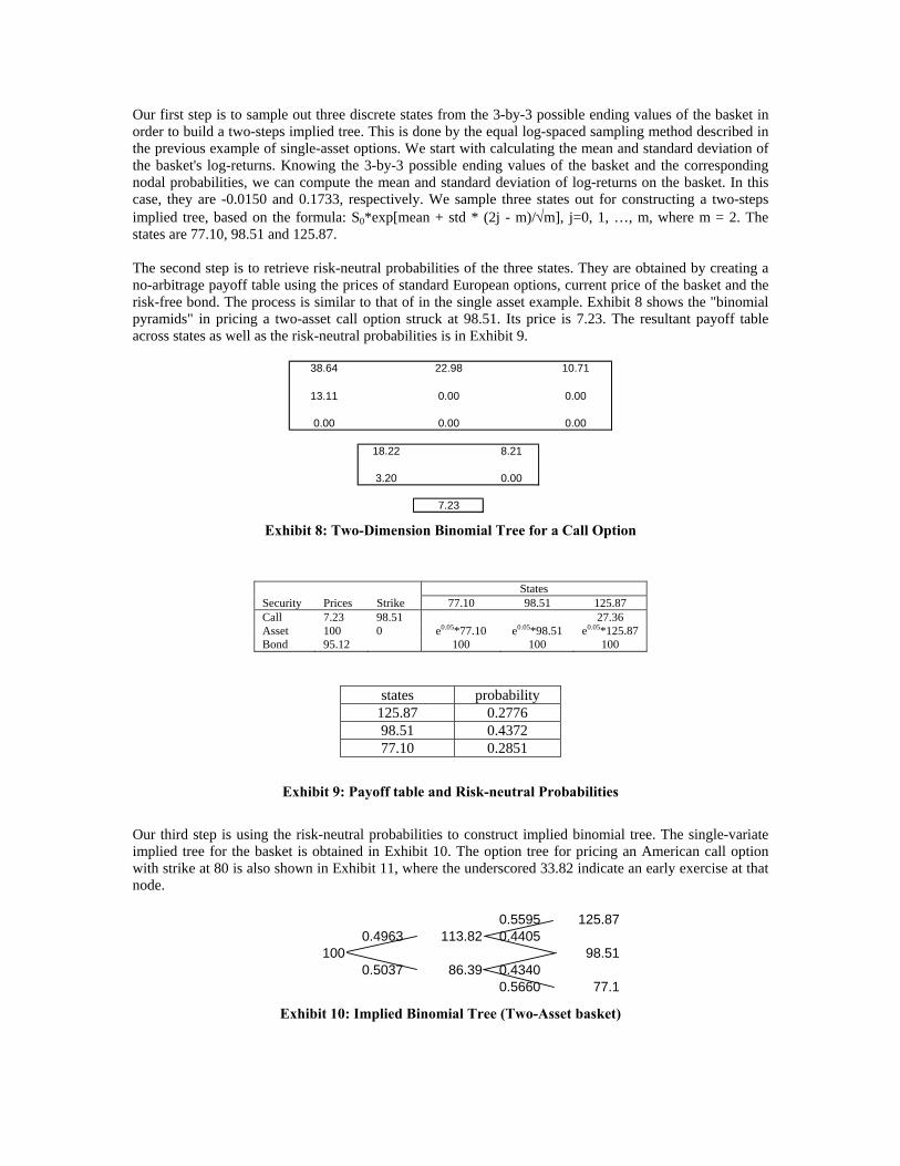
Two-asset options (Case 1) Time to Expiration: T = 1.0 year Interest Rate: r = 5% Dividend Yield: δ1 = 5%, δ2 = 5% Volatilities: σ1 = 20%, σ2 = 20% Correlation: ρ = 0.5 Spot Prices: S1,0 = 50, S2,0 = 50 # of shares: n1 = 1, n2 = 1 Strike Prices: K = 60, 70, 80, 90, 100, 110, 120, 130, 140. Risk-Neutral Probabilities
OptionStrike Put/Call Prices Risk-neutraNormal Diffs
45.374 P 0.0000 0.000006 0.000001 0.00000549.031 P 0.0000 0.000046 0.000019 0.00002752.983 P 0.0002 0.000296 0.000181 0.00011557.254 P 0.0016 0.001400 0.001087 0.00031361.869 P 0.0093 0.005262 0.004621 0.00064266.856 P 0.0426 0.015925 0.014786 0.00113972.245 P 0.1601 0.038520 0.036964 0.00155578.068 P 0.5005 0.073920 0.073929 -0.00000984.361 P 1.3109 0.118734 0.120134 -0.00140191.161 P 2.9545 0.160426 0.160179 0.00024798.509 C 7.2704 0.173841 0.176197 -0.002356
106.449 C 4.1614 0.158319 0.160179 -0.001860115.029 C 2.0939 0.118283 0.120134 -0.001851124.301 C 0.9031 0.075083 0.073929 0.001154134.321 C 0.3318 0.037622 0.036964 0.000658145.148 C 0.1019 0.015430 0.014786 0.000644156.847 C 0.0253 0.005195 0.004621 0.000575169.490 C 0.0049 0.001369 0.001087 0.000282183.152 C 0.0007 0.000279 0.000181 0.000097197.914 C 0.0001 0.000040 0.000019 0.000021213.867 C 0.0000 0.000005 0.000001 0.000004
Probabilitiesrisk-neutral probabilities
-0.020.000.020.040.060.080.100.120.140.160.180.20
45.37 57.25 72.25 91.16 115.03 145.15 183.15
Risk-neutralNormaldifference

Two-Asset Case(1) Steps: 10
Black-Scholes
Monte Carlo (10000)
LSMC (10000)
Black-Scholes
Monte Carlo (10000)
LSMC (10000)
Strike European European American European American European American Strike European European American European American European American60 38.0548 38.0838 40.0000 38.0516 39.9989 38.0556 40.0000 60 0.0056 0.0070 0.0076 0.0035 0.0035 0.0064 0.006470 28.6346 28.6681 30.0000 28.6265 29.9989 28.6407 30.0000 70 0.0977 0.1036 0.1068 0.0906 0.0909 0.1038 0.104080 19.7036 19.7583 20.2853 19.7062 20.2898 19.7712 20.3661 80 0.6790 0.7061 0.7134 0.6826 0.6854 0.7467 0.752890 12.0933 12.1895 12.3530 12.1395 12.3464 12.2862 12.5069 90 2.5810 2.6496 2.6731 2.6282 2.6480 2.7739 2.8037
100 6.5451 6.6550 6.7265 6.6109 6.6811 6.7430 6.8184 100 6.5451 6.6274 6.7020 6.6119 6.6872 6.7430 6.8443110 3.1330 3.2245 3.2624 3.1643 3.1863 3.1714 3.2049 110 12.6453 12.7092 12.8693 12.6776 12.8968 12.6837 12.9551120 1.3424 1.3939 1.4071 1.3355 1.3419 1.4995 1.5112 120 20.3669 20.3909 20.7954 20.3611 20.8665 20.5241 21.0382130 0.5229 0.5549 0.5667 0.5056 0.5073 0.6338 0.6364 130 29.0598 29.0642 30.0509 29.0435 30.0446 29.1707 30.1717140 0.1882 0.2016 0.2097 0.1671 0.1675 0.1990 0.1994 140 38.2373 38.2231 40.0000 38.2173 40.0011 38.2482 40.0000
Black-Scholes
Monte Carlo LSMC
Black-Scholes
Monte Carlo LSMC
Strike European European American European American European American Strike European European American European American European American60 0.0032 0.0322 0.0011 - - 0.0040 0.0011 60 0.0021 0.0035 0.0041 - - 0.0029 0.002970 0.0081 0.0416 0.0011 - - 0.0142 0.0011 70 0.0071 0.0130 0.0159 - - 0.0132 0.013180 -0.0026 0.0521 -0.0045 - - 0.0650 0.0763 80 -0.0036 0.0235 0.0280 - - 0.0641 0.067490 -0.0462 0.0500 0.0066 - - 0.1467 0.1605 90 -0.0472 0.0214 0.0251 - - 0.1457 0.1557
100 -0.0658 0.0441 0.0454 - - 0.1321 0.1373 100 -0.0668 0.0155 0.0148 - - 0.1311 0.1571110 -0.0313 0.0602 0.0761 - - 0.0071 0.0186 110 -0.0323 0.0316 -0.0275 - - 0.0061 0.0583120 0.0069 0.0584 0.0652 - - 0.1640 0.1693 120 0.0058 0.0298 -0.0711 - - 0.1630 0.1717130 0.0173 0.0493 0.0594 - - 0.1282 0.1291 130 0.0163 0.0207 0.0063 - - 0.1272 0.1271140 0.0211 0.0345 0.0422 - - 0.0319 0.0319 140 0.0200 0.0058 -0.0011 - - 0.0309 -0.0011
Call Options Put Options
Binomial Tree Implied Tree Binomial Tree Implied Tree
Implied Tree Binomial TreeBinomial Tree Implied Tree
Differences to the results from 2-D Binomial Tree Differences to the results from 2-D Binomial TreeCall Options Put Options
Two-Asset Case(1) Steps: 20
Black-Scholes
Monte Carlo (10000)
LSMC (10000)
Black-Scholes
Monte Carlo (10000)
LSMC (10000)
Strike European European American European American European American Strike European European American European American European American60 38.0548 38.0707 40.0000 38.0534 39.9995 38.0554 40.0000 60 0.0056 0.0068 0.0073 0.0047 0.0047 0.0062 0.006270 28.6346 28.6530 30.0000 28.6329 29.9995 28.6480 30.0000 70 0.0977 0.1014 0.1020 0.0966 0.0968 0.1111 0.111580 19.7037 19.7486 20.3362 19.7116 20.2899 19.7739 20.3535 80 0.6791 0.7093 0.7189 0.6875 0.6907 0.7493 0.753790 12.0934 12.1377 12.2812 12.1278 12.3405 12.1862 12.4160 90 2.5811 2.6107 2.6341 2.6160 2.6352 2.6739 2.6944
100 6.5453 6.5852 6.6563 6.5896 6.6627 6.6865 6.7629 100 6.5453 6.5706 6.6262 6.5901 6.6651 6.6865 6.7731110 3.1331 3.1798 3.2064 3.1651 3.1885 3.3058 3.3317 110 12.6454 12.6775 12.8411 12.6779 12.8942 12.8181 13.0436120 1.3425 1.3928 1.4225 1.3480 1.3553 1.4555 1.4642 120 20.3670 20.4027 20.9134 20.3731 20.8815 20.4801 20.9904130 0.5230 0.5448 0.5516 0.5179 0.5198 0.5781 0.5808 130 29.0599 29.0670 30.1083 29.0553 30.0721 29.1150 30.1276140 0.1882 0.1984 0.2023 0.1812 0.1817 0.2112 0.2120 140 38.2374 38.2329 40.0000 38.2309 40.0005 38.2604 40.0000
Black-Scholes
Monte Carlo LSMC
Black-Scholes
Monte Carlo LSMC
Strike European European American European American European American Strike European European American European American European American60 0.0014 0.0173 0.0005 - - 0.0020 0.0005 60 0.0009 0.0021 0.0026 - - 0.0015 0.001570 0.0017 0.0201 0.0005 - - 0.0151 0.0005 70 0.0011 0.0048 0.0052 - - 0.0145 0.014780 -0.0079 0.0370 0.0463 - - 0.0623 0.0636 80 -0.0084 0.0218 0.0282 - - 0.0618 0.063090 -0.0344 0.0099 -0.0593 - - 0.0584 0.0755 90 -0.0349 -0.0053 -0.0011 - - 0.0579 0.0592
100 -0.0443 -0.0044 -0.0064 - - 0.0969 0.1002 100 -0.0448 -0.0195 -0.0389 - - 0.0964 0.1080110 -0.0320 0.0147 0.0179 - - 0.1407 0.1432 110 -0.0325 -0.0004 -0.0531 - - 0.1402 0.1494120 -0.0055 0.0448 0.0672 - - 0.1075 0.1089 120 -0.0061 0.0296 0.0319 - - 0.1070 0.1089130 0.0051 0.0269 0.0318 - - 0.0602 0.0610 130 0.0046 0.0117 0.0362 - - 0.0597 0.0555140 0.0070 0.0172 0.0206 - - 0.0300 0.0303 140 0.0065 0.0020 -0.0005 - - 0.0295 -0.0005
Implied Tree Binomial Tree Implied Tree
Put Options
Binomial Tree Implied Tree Binomial Tree Implied Tree
Call Options
Binomial Tree
Differences to the results from 2-D Binomial Tree Differences to the results from 2-D Binomial TreeCall Options Put Options

Two-Asset Case(1) Steps: 50
Black-Scholes
Monte Carlo (10000)
LSMC (10000)
Black-Scholes
Monte Carlo (10000)
LSMC (10000)
Strike European European American European American European American Strike European European American European American European American60 38.0548 38.0677 40.0000 38.0544 39.9998 38.0548 40.0000 60 0.0057 0.0046 0.0056 0.0054 0.0054 0.0056 0.005670 28.6346 28.6521 30.0000 28.6351 29.9998 28.6363 30.0000 70 0.0977 0.1013 0.1022 0.0984 0.0987 0.0995 0.099980 19.7037 19.7422 20.3558 19.7117 20.2951 19.7308 20.3168 80 0.6791 0.7036 0.7038 0.6873 0.6906 0.7062 0.709790 12.0935 12.1623 12.2931 12.1163 12.3309 12.1442 12.3623 90 2.5812 2.6360 2.6335 2.6042 2.6235 2.6319 2.6532
100 6.5454 6.6260 6.6822 6.5741 6.6482 6.6331 6.7084 100 6.5454 6.6120 6.6656 6.5744 6.6492 6.6331 6.7110110 3.1332 3.2055 3.2258 3.1590 3.1829 3.1998 3.2245 110 12.6455 12.7038 12.8478 12.6715 12.8877 12.7121 12.9337120 1.3425 1.3902 1.3955 1.3560 1.3633 1.3591 1.3672 120 20.3671 20.4008 20.8416 20.3808 20.8880 20.3837 20.9027130 0.5230 0.5412 0.5571 0.5265 0.5286 0.5503 0.5528 130 29.0599 29.0641 30.1320 29.0636 30.0854 29.0872 30.1005140 0.1882 0.1943 0.2013 0.1886 0.1892 0.1938 0.1944 140 38.2374 38.2295 40.0000 38.2380 40.0002 38.2430 40.0000
Black-Scholes
Monte Carlo LSMC
Black-Scholes
Monte Carlo LSMC
Strike European European American European American European American Strike European European American European American European American60 0.0004 0.0133 0.0002 - - 0.0004 0.0002 60 0.0003 -0.0008 0.0002 - - 0.0002 0.000270 -0.0005 0.0170 0.0002 - - 0.0012 0.0002 70 -0.0007 0.0029 0.0035 - - 0.0011 0.001280 -0.0080 0.0305 0.0607 - - 0.0191 0.0217 80 -0.0082 0.0163 0.0132 - - 0.0189 0.019190 -0.0228 0.0460 -0.0378 - - 0.0279 0.0314 90 -0.0230 0.0318 0.0100 - - 0.0277 0.0297
100 -0.0287 0.0519 0.0340 - - 0.0590 0.0602 100 -0.0290 0.0376 0.0164 - - 0.0587 0.0618110 -0.0258 0.0465 0.0429 - - 0.0408 0.0416 110 -0.0260 0.0323 -0.0399 - - 0.0406 0.0460120 -0.0135 0.0342 0.0322 - - 0.0031 0.0039 120 -0.0137 0.0200 -0.0464 - - 0.0029 0.0147130 -0.0035 0.0147 0.0285 - - 0.0238 0.0242 130 -0.0037 0.0005 0.0466 - - 0.0236 0.0151140 -0.0004 0.0057 0.0121 - - 0.0052 0.0052 140 -0.0006 -0.0085 -0.0002 - - 0.0050 -0.0002
Implied Tree Binomial Tree Implied Tree
Differences to the results from 2-D Binomial Tree Differences to the results from 2-D Binomial Tree
Binomial Tree Implied Tree
Call Options Put Options
Call Options Put Options
Binomial Tree Implied Tree
Binomial Tree
Two-Asset Case(1) Steps:2 100
Black-Scholes
Monte Carlo (10000)
LSMC (10000)
Black-Scholes
Monte Carlo (10000)
LSMC (10000)
Strike European European American European American European American Strike European European American European American European American60 38.0548 38.0677 40.0000 38.0547 39.9999 38.0551 40.0000 60 0.0057 0.0046 0.0056 0.0057 0.0057 0.0059 0.005970 28.6346 28.6521 30.0000 28.6360 29.9999 28.6379 30.0000 70 0.0978 0.1013 0.1022 0.0992 0.0995 0.1010 0.101380 19.7037 19.7422 20.3558 19.7123 20.2962 19.7126 20.3013 80 0.6791 0.7036 0.7038 0.6878 0.6911 0.6880 0.691590 12.0935 12.1623 12.2931 12.1148 12.3297 12.1389 12.3548 90 2.5812 2.6360 2.6335 2.6026 2.6217 2.6266 2.6463
100 6.5454 6.6260 6.6822 6.5740 6.6480 6.6055 6.6804 100 6.5454 6.6120 6.6656 6.5741 6.6485 6.6055 6.6810110 3.1332 3.2055 3.2258 3.1578 3.1818 3.1744 3.1989 110 12.6455 12.7038 12.8478 12.6702 12.8860 12.6867 12.9057120 1.3425 1.3902 1.3955 1.3575 1.3648 1.3752 1.3830 120 20.3671 20.4008 20.8416 20.3822 20.8890 20.3998 20.9077130 0.5230 0.5412 0.5571 0.5303 0.5324 0.5303 0.5327 130 29.0599 29.0641 30.1320 29.0673 30.0870 29.0672 30.0923140 0.1882 0.1943 0.2013 0.1908 0.1914 0.1932 0.1938 140 38.2374 38.2295 40.0000 38.2400 40.0001 38.2424 40.0000
Black-Scholes
Monte Carlo LSMC
Black-Scholes
Monte Carlo LSMC
Strike European European American European American European American Strike European European American European American European American60 0.0001 0.0130 0.0001 - - 0.0004 0.0001 60 0.0000 -0.0011 -0.0001 - - 0.0002 0.000270 -0.0014 0.0161 0.0001 - - 0.0019 0.0001 70 -0.0014 0.0021 0.0027 - - 0.0018 0.001880 -0.0086 0.0299 0.0596 - - 0.0003 0.0051 80 -0.0087 0.0158 0.0127 - - 0.0002 0.000490 -0.0213 0.0475 -0.0366 - - 0.0241 0.0251 90 -0.0214 0.0334 0.0118 - - 0.0240 0.0246
100 -0.0286 0.0520 0.0342 - - 0.0315 0.0324 100 -0.0287 0.0379 0.0171 - - 0.0314 0.0325110 -0.0246 0.0477 0.0440 - - 0.0166 0.0171 110 -0.0247 0.0336 -0.0382 - - 0.0165 0.0197120 -0.0150 0.0327 0.0307 - - 0.0177 0.0182 120 -0.0151 0.0186 -0.0474 - - 0.0176 0.0187130 -0.0073 0.0109 0.0247 - - 0.0000 0.0003 130 -0.0074 -0.0032 0.0450 - - -0.0001 0.0053140 -0.0026 0.0035 0.0099 - - 0.0024 0.0024 140 -0.0026 -0.0105 -0.0001 - - 0.0024 -0.0001
Implied Tree Binomial Tree Implied Tree
Differences to the results from 2-D Binomial Tree Differences to the results from 2-D Binomial Tree
Binomial Tree
Binomial Tree Implied Tree Binomial Tree Implied Tree
Call Options Put Options
Call Options Put Options
2 50 steps are applied to both Monte Carlo simulation and the Least Squares Monte Carlo.

Two-asset options (Case 2) Time to Expiration: T = 1.0 year Interest Rate: r = 5% Dividend Yield: δ1 = 5%, δ2 = 5% Volatilities: σ1 = 20%, σ2 = 90% Correlation: ρ = -0.9 Spot Prices: S1,0 = 50, S2,0 = 50 # of shares: n1 = 1, n2 = 1 Strike Prices: K = 60, 70, 80, 90, 100, 110, 120, 130, 140. Risk-Neutral Probabilities
OptionStrike Put/Call Prices Risk-neutraNormal Diffs
21.884 P 0.0000 0.000000 0.000001 -0.00000125.306 P 0.0000 0.000000 0.000019 -0.00001929.262 P 0.0000 0.000000 0.000181 -0.00018133.837 P 0.0000 0.000000 0.001087 -0.00108739.128 P 0.0000 0.000000 0.004621 -0.00462145.246 P 0.0000 0.000000 0.014786 -0.01478652.320 P 0.0000 0.000123 0.036964 -0.03684160.500 P 0.0010 0.025021 0.073929 -0.04890869.959 P 0.2272 0.229349 0.120134 0.10921580.897 P 2.8751 0.291802 0.160179 0.13162393.545 C 15.5879 0.167917 0.176197 -0.008280
108.171 C 11.6119 0.096203 0.160179 -0.063977125.083 C 8.5619 0.065523 0.120134 -0.054611144.640 C 6.2540 0.042088 0.073929 -0.031841167.254 C 4.4907 0.028615 0.036964 -0.008350193.404 C 3.1634 0.019361 0.014786 0.004575223.643 C 2.1854 0.012758 0.004621 0.008137258.609 C 1.4789 0.008220 0.001087 0.007133299.043 C 0.9782 0.005197 0.000181 0.005016345.798 C 0.6302 -0.004431 0.000019 -0.004450399.863 C 0.3939 0.012254 0.000001 0.012254
Probabilitiesrisk-neutral probabilities
-0.10-0.050.000.050.100.150.200.250.300.35
21.88 33.84 52.32 80.90 125.08 193.40 299.04
Risk-neutralNormaldifference

Two-Asset Case(2) Steps: 10
Black-Scholes
Monte Carlo (10000)
LSMC (10000)
Black-Scholes
Monte Carlo (10000)
LSMC (10000)
Strike European European American European American European American Strike European European American European American European American60 38.5961 37.9077 40.0000 37.8723 39.8136 38.8215 40.8092 60 0.5470 0.0014 0.0014 0.0004 0.0004 0.0026 0.002670 30.2163 28.6341 30.0000 28.5876 29.8136 30.0214 30.9306 70 1.6794 0.2400 0.2423 0.2281 0.2288 0.7148 0.716280 22.8939 21.4239 21.9614 21.3935 21.8086 22.8136 23.3034 80 3.8693 2.5421 2.5397 2.5463 2.5601 3.0193 3.037690 16.8366 16.8052 17.3085 16.7687 16.9846 17.9410 18.3225 90 7.3243 7.4358 7.4456 7.4337 7.5016 7.6590 7.6967
100 12.0665 13.5824 13.9667 13.5230 13.6573 14.5383 14.7980 100 12.0665 13.7252 13.8238 13.7004 13.8716 13.7686 13.9295110 8.4634 11.1848 11.5379 11.1016 11.1955 11.9509 12.1742 110 17.9757 20.8399 21.0792 20.7912 21.0937 20.6935 20.9912120 5.8329 9.3422 9.6220 9.2592 9.3227 9.9571 10.1153 120 24.8575 28.5096 28.8986 28.4611 28.9349 28.2120 28.7971130 3.9641 7.8862 8.1123 7.7166 7.7683 8.5140 8.6479 130 32.5009 36.5659 37.1190 36.4308 37.1321 36.2812 37.1421140 2.6646 6.7407 6.9911 6.5877 6.6222 7.0709 7.1850 140 40.7137 44.9327 45.7550 44.8142 45.7414 44.3504 45.7046
Black-Scholes
Monte Carlo LSMC
Black-Scholes
Monte Carlo LSMC
Strike European European American European American European American Strike European European American European American European American60 0.7238 0.0354 0.1864 - - 0.9492 0.9956 60 0.5466 0.0010 0.0010 - - 0.0022 0.002270 1.6287 0.0465 0.1864 - - 1.4338 1.1170 70 1.4513 0.0119 0.0135 - - 0.4867 0.487480 1.5004 0.0304 0.1528 - - 1.4201 1.4948 80 1.3230 -0.0042 -0.0204 - - 0.4730 0.477590 0.0679 0.0365 0.3239 - - 1.1723 1.3379 90 -0.1094 0.0021 -0.0560 - - 0.2253 0.1951
100 -1.4565 0.0594 0.3094 - - 1.0153 1.1407 100 -1.6339 0.0248 -0.0478 - - 0.0682 0.0579110 -2.6382 0.0832 0.3424 - - 0.8493 0.9787 110 -2.8155 0.0487 -0.0145 - - -0.0977 -0.1025120 -3.4263 0.0830 0.2993 - - 0.6979 0.7926 120 -3.6036 0.0485 -0.0363 - - -0.2491 -0.1378130 -3.7525 0.1696 0.3440 - - 0.7974 0.8796 130 -3.9299 0.1351 -0.0131 - - -0.1496 0.0100140 -3.9231 0.1530 0.3689 - - 0.4832 0.5628 140 -4.1005 0.1185 0.0136 - - -0.4638 -0.0368
Implied Tree
Differences to the results from 2-D Binomial Tree Differences to the results from 2-D Binomial TreeCall Options Put Options
Binomial Tree Binomial TreeImplied Tree
Call Options Put Options
Binomial Tree Implied Tree Binomial Tree Implied Tree
Two-Asset Case(2) Steps: 20
Black-Scholes
Monte Carlo (10000)
LSMC (10000)
Black-Scholes
Monte Carlo (10000)
LSMC (10000)
Strike European European American European American European American Strike European European American European American European American60 38.6064 38.8562 40.0289 37.9604 39.9059 39.0816 41.0844 60 0.5572 0.0005 0.0007 0.0007 0.0007 0.0009 0.000970 30.2375 29.5706 30.1782 28.6785 29.9059 29.8045 31.0844 70 1.7006 0.2272 0.2302 0.2311 0.2318 0.2361 0.237380 22.9269 22.3005 22.4821 21.4695 21.8971 22.7023 23.2447 80 3.9023 2.4694 2.4843 2.5344 2.5478 2.6463 2.652090 16.8788 17.6760 17.6119 16.8502 17.0779 18.1158 18.4949 90 7.3665 7.3572 7.4382 7.4274 7.4931 7.5720 7.6105
100 12.1134 14.4648 14.6292 13.6274 13.7736 14.8036 15.0945 100 12.1134 13.6583 13.8031 13.7169 13.8788 13.7721 13.9084110 8.5104 12.0520 12.1744 11.2076 11.3091 12.2218 12.4580 110 18.0227 20.7578 21.0248 20.8094 21.1071 20.7026 21.0271120 5.8765 10.1882 10.3079 9.3527 9.4273 10.3844 10.5815 120 24.9010 28.4063 28.8076 28.4668 28.9334 28.3775 28.9174130 4.0021 8.6936 8.8717 7.9032 7.9583 8.8521 9.0144 130 32.5389 36.4240 37.0295 36.5295 37.2041 36.3575 37.2168140 2.6963 7.4864 7.7061 6.6953 6.7372 7.6352 7.7749 140 40.7454 44.7290 45.5608 44.8339 45.7603 44.6529 45.8534
Black-Scholes
Monte Carlo LSMC
Black-Scholes
Monte Carlo LSMC
Strike European European American European American European American Strike European European American European American European American60 0.6460 0.8958 0.1230 - - 1.1212 1.1785 60 0.5565 -0.0002 0.0000 - - 0.0002 0.000270 1.5590 0.8921 0.2723 - - 1.1260 1.1785 70 1.4695 -0.0039 -0.0016 - - 0.0050 0.005580 1.4574 0.8310 0.5850 - - 1.2328 1.3476 80 1.3679 -0.0650 -0.0635 - - 0.1119 0.104290 0.0286 0.8258 0.5340 - - 1.2656 1.4170 90 -0.0609 -0.0702 -0.0549 - - 0.1446 0.1174
100 -1.5140 0.8374 0.8556 - - 1.1762 1.3209 100 -1.6035 -0.0586 -0.0757 - - 0.0552 0.0296110 -2.6972 0.8444 0.8653 - - 1.0142 1.1489 110 -2.7867 -0.0516 -0.0823 - - -0.1068 -0.0800120 -3.4762 0.8355 0.8806 - - 1.0317 1.1542 120 -3.5658 -0.0605 -0.1258 - - -0.0893 -0.0160130 -3.9011 0.7904 0.9134 - - 0.9489 1.0561 130 -3.9906 -0.1055 -0.1746 - - -0.1720 0.0127140 -3.9990 0.7911 0.9689 - - 0.9399 1.0377 140 -4.0885 -0.1049 -0.1995 - - -0.1810 0.0931
Differences to the results from 2-D Binomial Tree Differences to the results from 2-D Binomial TreeCall Options Put Options
Binomial Tree Implied Tree Binomial Tree Implied Tree
Call Options Put Options
Binomial Tree Implied Tree Binomial Tree Implied Tree

Two-Asset Case(2) Steps: 50
Black-Scholes
Monte Carlo (10000)
LSMC (10000)
Black-Scholes
Monte Carlo (10000)
LSMC (10000)
Strike European European American European American European American Strike European European American European American European American60 38.6125 38.1226 40.0000 38.0140 39.9622 38.2001 40.1543 60 0.5633 0.0006 0.0008 0.0009 0.0009 0.0041 0.004170 30.2500 28.8574 30.0514 28.7350 29.9622 28.9624 30.1543 70 1.7132 0.2477 0.2470 0.2341 0.2346 0.2788 0.279180 22.9463 21.6275 21.6520 21.5129 21.9479 21.8443 22.3232 80 3.9217 2.5301 2.5348 2.5243 2.5369 2.6730 2.680390 16.9036 17.0169 17.4222 16.9016 17.1386 17.1734 17.5148 90 7.3913 7.4317 7.4566 7.4253 7.4878 7.5144 7.5507
100 12.1410 13.8171 14.0481 13.6859 13.8384 13.8978 14.1658 100 12.1410 13.7443 13.8219 13.7219 13.8790 13.7511 13.8795110 8.5380 11.4360 11.7531 11.2836 11.3899 11.4784 11.6952 110 18.0503 20.8755 21.0542 20.8319 21.1214 20.8440 21.1415120 5.9021 9.5986 9.8586 9.4312 9.5089 9.6205 9.7989 120 24.9267 28.5504 28.9479 28.4917 28.9506 28.4983 29.0335130 4.0245 8.1287 8.3996 7.9678 8.0267 8.1572 8.3053 130 32.5613 36.5927 37.1226 36.5406 37.2062 36.5474 37.3779140 2.7149 6.9352 7.1374 6.7951 6.8409 6.9757 7.1002 140 40.7641 44.9115 45.6813 44.8802 45.7881 44.8782 46.0534
Black-Scholes
Monte Carlo LSMC
Black-Scholes
Monte Carlo LSMC
Strike European European American European American European American Strike European European American European American European American60 0.5985 0.1086 0.0378 - - 0.1861 0.1921 60 0.5624 -0.0003 -0.0001 - - 0.0032 0.003270 1.5150 0.1224 0.0892 - - 0.2274 0.1921 70 1.4791 0.0136 0.0124 - - 0.0447 0.044580 1.4334 0.1146 -0.2959 - - 0.3314 0.3753 80 1.3974 0.0058 -0.0021 - - 0.1487 0.143490 0.0020 0.1153 0.2836 - - 0.2718 0.3762 90 -0.0340 0.0064 -0.0312 - - 0.0891 0.0629
100 -1.5449 0.1312 0.2097 - - 0.2119 0.3274 100 -1.5809 0.0224 -0.0571 - - 0.0292 0.0005110 -2.7456 0.1524 0.3632 - - 0.1948 0.3053 110 -2.7816 0.0436 -0.0672 - - 0.0121 0.0201120 -3.5291 0.1674 0.3497 - - 0.1893 0.2900 120 -3.5650 0.0587 -0.0027 - - 0.0066 0.0829130 -3.9433 0.1609 0.3729 - - 0.1894 0.2786 130 -3.9793 0.0521 -0.0836 - - 0.0068 0.1717140 -4.0802 0.1401 0.2965 - - 0.1806 0.2593 140 -4.1161 0.0313 -0.1068 - - -0.0020 0.2653
Implied Tree
Differences to the results from 2-D Binomial Tree Differences to the results from 2-D Binomial TreeCall Options Put Options
Binomial Tree Implied Tree Binomial Tree
Call Options Put Options
Binomial Tree Implied Tree Binomial Tree Implied Tree
Two-Asset Case(2) Steps:3 100
Black-Scholes
Monte Carlo (10000)
LSMC (10000)
Black-Scholes
Monte Carlo (10000)
LSMC (10000)
Strike European European American European American European American Strike European European American European American European American60 38.6145 38.1226 40.0000 38.0321 39.9810 38.0553 40.0041 60 0.5653 0.0006 0.0008 0.0009 0.0009 0.0022 0.002270 30.2542 28.8574 30.0514 28.7545 29.9810 28.8327 30.0041 70 1.7173 0.2477 0.2470 0.2357 0.2362 0.2919 0.292280 22.9527 21.6275 21.6520 21.5287 21.9681 21.6414 22.1147 80 3.9281 2.5301 2.5348 2.5221 2.5343 2.6129 2.617690 16.9118 17.0169 17.4222 16.9171 17.1569 16.9861 17.3200 90 7.3995 7.4317 7.4566 7.4228 7.4843 7.4699 7.5049
100 12.1501 13.8171 14.0481 13.7043 13.8588 13.7125 13.9741 100 12.1501 13.7443 13.8219 13.7223 13.8777 13.7086 13.8408110 8.5472 11.4360 11.7531 11.3052 11.4130 11.3436 11.5541 110 18.0595 20.8755 21.0542 20.8355 21.1223 20.8520 21.1473120 5.9105 9.5986 9.8586 9.4542 9.5333 9.4759 9.6493 120 24.9351 28.5504 28.9479 28.4969 28.9525 28.4966 29.0302130 4.0319 8.1287 8.3996 7.9951 8.0550 8.0039 8.1481 130 32.5687 36.5927 37.1226 36.5500 37.2112 36.5369 37.3672140 2.7211 6.9352 7.1374 6.8227 6.8693 6.8411 6.9619 140 40.7703 44.9115 45.6813 44.8900 45.7929 44.8864 46.0523
Black-Scholes
Monte Carlo LSMC
Black-Scholes
Monte Carlo LSMC
Strike European European American European American European American Strike European European American European American European American60 0.5824 0.0905 0.0190 - - 0.0232 0.0231 60 0.5644 -0.0003 -0.0001 - - 0.0013 0.001370 1.4997 0.1029 0.0704 - - 0.0782 0.0231 70 1.4816 0.0120 0.0108 - - 0.0562 0.056080 1.4240 0.0988 -0.3161 - - 0.1127 0.1466 80 1.4060 0.0080 0.0005 - - 0.0908 0.083390 -0.0053 0.0998 0.2653 - - 0.0690 0.1631 90 -0.0233 0.0089 -0.0277 - - 0.0471 0.0206
100 -1.5542 0.1128 0.1893 - - 0.0082 0.1153 100 -1.5722 0.0220 -0.0558 - - -0.0137 -0.0369110 -2.7580 0.1308 0.3401 - - 0.0384 0.1411 110 -2.7760 0.0400 -0.0681 - - 0.0165 0.0250120 -3.5437 0.1444 0.3253 - - 0.0217 0.1160 120 -3.5618 0.0535 -0.0046 - - -0.0003 0.0777130 -3.9632 0.1336 0.3446 - - 0.0088 0.0931 130 -3.9813 0.0427 -0.0886 - - -0.0131 0.1560140 -4.1016 0.1125 0.2681 - - 0.0184 0.0926 140 -4.1197 0.0215 -0.1116 - - -0.0036 0.2594
Implied Tree Binomial Tree Implied Tree
Differences to the results from 2-D Binomial Tree Differences to the results from 2-D Binomial TreeCall Options Put Options
Call Options Put Options
Binomial Tree
Binomial Tree Implied Tree Binomial Tree Implied Tree
3 50 steps are applied to both Monte Carlo simulation and the Least Squares Monte Carlo.

Three-asset options (Case 1) Time to Expiration: T = 1.0 year Interest Rate: r = 5% Dividend Yield: δ1 = 5%, δ2 = 5%, δ3 = 5% Volatilities: σ1 = 20%, σ2 = 20%, σ2 = 20% Correlation:
⎥⎥⎥
⎦
⎤
⎢⎢⎢
⎣
⎡
15.05.05.015.05.05.01
Spot Prices: S1,0 = 33.33, S2,0 = 33.33, S3,0 = 33.33 # of shares: n1 = 1, n2 = 1, n3 = 1 Strike Prices: K = 60, 70, 80, 90, 100, 110, 120, 130, 140. Risk-Neutral Probabilities
OptionStrike Put/Call Prices Risk-neutraNormal Diffs
47.511 P 0.0000 0.000007 0.000001 0.00000651.113 P 0.0000 0.000049 0.000019 0.00003054.989 P 0.0002 0.000308 0.000181 0.00012759.158 P 0.0017 0.001439 0.001087 0.00035263.644 P 0.0094 0.005353 0.004621 0.00073368.469 P 0.0422 0.015798 0.014786 0.00101273.661 P 0.1556 0.037933 0.036964 0.00096979.246 P 0.4791 0.074482 0.073929 0.00055385.255 P 1.2528 0.119255 0.120134 -0.00087991.719 P 2.8185 0.159259 0.160179 -0.00092098.673 C 6.8183 0.174020 0.176197 -0.002177
106.155 C 3.8855 0.158922 0.160179 -0.001257114.204 C 1.9471 0.119019 0.120134 -0.001115122.863 C 0.8421 0.074068 0.073929 0.000139132.179 C 0.3096 0.037595 0.036964 0.000630142.201 C 0.0952 0.015544 0.014786 0.000758152.984 C 0.0239 0.005220 0.004621 0.000599164.583 C 0.0048 0.001385 0.001087 0.000298177.062 C 0.0008 0.000291 0.000181 0.000110190.488 C 0.0001 0.000046 0.000019 0.000027204.931 C 0.0000 0.000007 0.000001 0.000006
Probabilitiesrisk-neutral probabilities
-0.020.000.020.040.060.080.100.120.140.160.180.20
47.51 59.16 73.66 91.72 114.20 142.20 177.06
Risk-neutralNormaldifference
Three-Asset Case(1) Steps: 10
Black-Scholes
Monte Carlo (10000)
LSMC (10000)
Black-Scholes
Monte Carlo (10000)
LSMC (10000)
Strike European European American European American European American Strike European European American European American European American60 38.0520 38.0586 40.0000 38.0502 39.9991 38.0518 40.0000 60 0.0028 0.0027 0.0032 0.0019 0.0019 0.0026 0.002670 28.6021 28.6086 30.0000 28.5968 29.9991 28.6163 30.0000 70 0.0652 0.0650 0.0668 0.0608 0.0609 0.0794 0.079680 19.5664 19.5821 20.1410 19.5705 20.1736 19.5812 20.2386 80 0.5418 0.5508 0.5542 0.5468 0.5488 0.5566 0.559090 11.8041 11.8433 11.9634 11.8340 12.0422 11.9351 12.1601 90 2.2918 2.3243 2.3437 2.3226 2.3381 2.4228 2.4497
100 6.1739 6.2221 6.2533 6.2193 6.2850 6.3537 6.4250 100 6.1739 6.2153 6.2609 6.2202 6.2884 6.3537 6.4495110 2.8018 2.8433 2.8766 2.8255 2.8442 2.8736 2.8962 110 12.3141 12.3489 12.4909 12.3387 12.5506 12.3859 12.6498120 1.1173 1.1353 1.1511 1.1134 1.1183 1.1968 1.2068 120 20.1419 20.1532 20.6092 20.1389 20.6604 20.2214 20.7700130 0.3986 0.4050 0.4095 0.3839 0.3850 0.4837 0.4859 130 28.9354 28.9351 30.0000 28.9217 30.0009 29.0206 30.0683140 0.1295 0.1299 0.1346 0.1160 0.1162 0.1551 0.1554 140 38.1787 38.1724 40.0000 38.1661 40.0009 38.2042 40.0000
Black-Scholes
Monte Carlo LSMC
Black-Scholes
Monte Carlo LSMC
Strike European European American European American European American Strike European European American European American European American60 0.0018 0.0084 0.0009 - - 0.0016 0.0009 60 0.0009 0.0008 0.0013 - - 0.0007 0.000770 0.0053 0.0118 0.0009 - - 0.0195 0.0009 70 0.0044 0.0042 0.0059 - - 0.0186 0.018780 -0.0041 0.0116 -0.0326 - - 0.0107 0.0650 80 -0.0050 0.0040 0.0054 - - 0.0098 0.010290 -0.0299 0.0093 -0.0788 - - 0.1011 0.1179 90 -0.0308 0.0017 0.0056 - - 0.1002 0.1116
100 -0.0454 0.0028 -0.0317 - - 0.1344 0.1400 100 -0.0463 -0.0049 -0.0275 - - 0.1335 0.1611110 -0.0237 0.0178 0.0324 - - 0.0481 0.0520 110 -0.0246 0.0102 -0.0597 - - 0.0472 0.0992120 0.0039 0.0219 0.0328 - - 0.0834 0.0885 120 0.0030 0.0143 -0.0512 - - 0.0825 0.1096130 0.0147 0.0211 0.0245 - - 0.0998 0.1009 130 0.0137 0.0134 -0.0009 - - 0.0989 0.0674140 0.0135 0.0139 0.0184 - - 0.0391 0.0392 140 0.0126 0.0063 -0.0009 - - 0.0381 -0.0009
Implied Tree
Call Options Put Options
Binomial Tree Implied Tree Binomial Tree Implied Tree
Binomial Tree Binomial TreeImplied Tree
Differences to the results from 3-D Binomial Tree Differences to the results from 3-D Binomial TreeCall Options Put Options

Three-Asset Case(1) Steps: 20
Black-Scholes
Monte Carlo (10000)
LSMC (10000)
Black-Scholes
Monte Carlo (10000)
LSMC (10000)
Strike European European American European American European American Strike European European American European American European American60 38.0520 38.0352 40.0000 38.0511 39.9995 38.0523 40.0000 60 0.0028 0.0021 0.0026 0.0024 0.0024 0.0031 0.003170 28.6021 28.5853 30.0000 28.6003 29.9995 28.6125 30.0000 70 0.0652 0.0645 0.0686 0.0639 0.0640 0.0757 0.075980 19.5665 19.5432 20.2169 19.5722 20.1809 19.6007 20.2151 80 0.5419 0.5347 0.5374 0.5480 0.5503 0.5762 0.579990 11.8043 11.7616 12.0321 11.8287 12.0411 11.9144 12.1409 90 2.2920 2.2655 2.3085 2.3168 2.3330 2.4021 2.4198
100 6.1742 6.1366 6.2579 6.2062 6.2743 6.2983 6.3704 100 6.1742 6.1527 6.2535 6.2066 6.2761 6.2983 6.3801110 2.8021 2.7660 2.8128 2.8237 2.8437 2.9596 2.9829 110 12.3144 12.2944 12.5441 12.3364 12.5506 12.4719 12.6951120 1.1175 1.1010 1.1098 1.1221 1.1275 1.2075 1.2150 120 20.1421 20.1417 20.7009 20.1471 20.6705 20.2321 20.7593130 0.3987 0.4001 0.4111 0.3950 0.3963 0.4342 0.4364 130 28.9355 28.9531 30.0050 28.9323 30.0040 28.9711 30.0416140 0.1296 0.1291 0.1407 0.1242 0.1245 0.1423 0.1429 140 38.1787 38.1944 40.0000 38.1739 40.0005 38.1915 40.0000
Black-Scholes
Monte Carlo LSMC
Black-Scholes
Monte Carlo LSMC
Strike European European American European American European American Strike European European American European American European American60 0.0009 -0.0159 0.0005 - - 0.0012 0.0005 60 0.0004 -0.0003 0.0002 - - 0.0007 0.000770 0.0018 -0.0150 0.0005 - - 0.0122 0.0005 70 0.0013 0.0006 0.0046 - - 0.0118 0.011980 -0.0057 -0.0290 0.0360 - - 0.0285 0.0342 80 -0.0061 -0.0133 -0.0129 - - 0.0282 0.029690 -0.0244 -0.0671 -0.0090 - - 0.0857 0.0998 90 -0.0248 -0.0513 -0.0245 - - 0.0853 0.0868
100 -0.0320 -0.0696 -0.0164 - - 0.0921 0.0961 100 -0.0324 -0.0539 -0.0226 - - 0.0917 0.1040110 -0.0216 -0.0577 -0.0309 - - 0.1359 0.1392 110 -0.0220 -0.0420 -0.0065 - - 0.1355 0.1445120 -0.0046 -0.0211 -0.0177 - - 0.0854 0.0875 120 -0.0050 -0.0054 0.0304 - - 0.0850 0.0888130 0.0037 0.0051 0.0148 - - 0.0392 0.0401 130 0.0032 0.0208 0.0010 - - 0.0388 0.0376140 0.0054 0.0049 0.0162 - - 0.0181 0.0184 140 0.0048 0.0205 -0.0005 - - 0.0176 -0.0005
Differences to the results from 3-D Binomial Tree Differences to the results from 3-D Binomial TreeCall Options Put Options
Binomial Tree Implied Tree Binomial Tree Implied Tree
Call Options Put Options
Binomial Tree Implied Tree Binomial Tree Implied Tree
Three-Asset Case(1) Steps: 30
Black-Scholes
Monte Carlo (10000)
LSMC (10000)
Black-Scholes
Monte Carlo (10000)
LSMC (10000)
Strike European European American European American European American Strike European European American European American European American60 38.0520 38.0492 40.0000 38.0514 39.9997 38.0522 40.0000 60 0.0028 0.0028 0.0034 0.0026 0.0026 0.0030 0.003070 28.6021 28.6038 30.0000 28.6014 29.9997 28.6086 30.0000 70 0.0652 0.0697 0.0751 0.0648 0.0650 0.0717 0.072080 19.5665 19.5688 20.2416 19.5722 20.1838 19.6092 20.2201 80 0.5420 0.5470 0.5475 0.5479 0.5503 0.5846 0.587590 11.8044 11.7979 12.0296 11.8249 12.0387 11.9046 12.1225 90 2.2921 2.2884 2.3026 2.3129 2.3293 2.3923 2.4108
100 6.1744 6.1488 6.2112 6.2023 6.2711 6.2738 6.3452 100 6.1744 6.1516 6.2085 6.2026 6.2724 6.2738 6.3508110 2.8022 2.8028 2.8100 2.8226 2.8431 2.8786 2.9032 110 12.3145 12.3179 12.5577 12.3352 12.5499 12.3909 12.6114120 1.1176 1.1293 1.1443 1.1255 1.1311 1.1715 1.1776 120 20.1422 20.1567 20.7089 20.1504 20.6744 20.1960 20.7302130 0.3987 0.4119 0.4191 0.3985 0.4000 0.4310 0.4329 130 28.9356 28.9516 30.0756 28.9357 30.0143 28.9679 30.0417140 0.1296 0.1387 0.1490 0.1272 0.1275 0.1357 0.1363 140 38.1788 38.1907 40.0000 38.1767 40.0003 38.1849 40.0000
Black-Scholes
Monte Carlo LSMC
Black-Scholes
Monte Carlo LSMC
Strike European European American European American European American Strike European European American European American European American60 0.0006 -0.0022 0.0003 - - 0.0008 0.0003 60 0.0002 0.0002 0.0008 - - 0.0004 0.000470 0.0007 0.0024 0.0003 - - 0.0072 0.0003 70 0.0004 0.0049 0.0101 - - 0.0069 0.007080 -0.0057 -0.0034 0.0578 - - 0.0370 0.0363 80 -0.0059 -0.0009 -0.0028 - - 0.0367 0.037290 -0.0205 -0.0270 -0.0091 - - 0.0797 0.0838 90 -0.0208 -0.0245 -0.0267 - - 0.0794 0.0815
100 -0.0279 -0.0535 -0.0599 - - 0.0715 0.0741 100 -0.0282 -0.0510 -0.0639 - - 0.0712 0.0784110 -0.0204 -0.0198 -0.0331 - - 0.0560 0.0601 110 -0.0207 -0.0173 0.0078 - - 0.0557 0.0615120 -0.0079 0.0038 0.0132 - - 0.0460 0.0465 120 -0.0082 0.0063 0.0345 - - 0.0456 0.0558130 0.0002 0.0134 0.0191 - - 0.0325 0.0329 130 -0.0001 0.0159 0.0613 - - 0.0322 0.0274140 0.0024 0.0115 0.0215 - - 0.0085 0.0088 140 0.0021 0.0140 -0.0003 - - 0.0082 -0.0003
Differences to the results from 3-D Binomial Tree
Implied Tree Binomial Tree Implied Tree
Binomial Tree Implied Tree
Differences to the results from 3-D Binomial Tree
Implied Tree
Call Options Put Options
Call Options Put Options
Binomial Tree
Binomial Tree

Three-asset options (Case 2) Time to Expiration: T = 1.0 year Interest Rate: r = 5% Dividend Yield: δ1 = 5%, δ2 = 5%, δ3 = 5% Volatilities: σ1 = 20%, σ2 = 90%, σ2 = 90% Correlation:
⎥⎥⎥
⎦
⎤
⎢⎢⎢
⎣
⎡
19.09.09.019.09.09.01
Spot Prices: S1,0 = 33.33, S2,0 = 33.33, S3,0 = 33.33 # of shares: n1 = 1, n2 = 1, n3 = 1 Strike Prices: K = 60, 70, 80, 90, 100, 110, 120, 130, 140. Risk-Neutral Probabilities
OptionStrike Put/Call Prices Risk-neutral Normal Diffs
5.958 P 0.0000 0.000000 0.000001 -0.0000017.750 P 0.0000 0.000000 0.000019 -0.000019
10.080 P 0.0000 0.000000 0.000181 -0.00018113.110 P 0.0000 0.000004 0.001087 -0.00108317.051 P 0.0000 0.000404 0.004621 -0.00421722.178 P 0.0020 0.006475 0.014786 -0.00831128.846 P 0.0457 0.034150 0.036964 -0.00281437.518 P 0.3841 0.088915 0.073929 0.01498648.798 P 1.7784 0.145935 0.120134 0.02580163.468 P 5.6285 0.169199 0.160179 0.00902082.550 C 30.3060 0.176776 0.176197 0.000579
107.368 C 21.3789 0.140165 0.160179 -0.020014139.648 C 14.0716 0.101042 0.120134 -0.019092181.633 C 8.6028 0.064885 0.073929 -0.009044236.240 C 4.8602 0.037476 0.036964 0.000512307.265 C 2.5243 0.019449 0.014786 0.004664399.643 C 1.1952 0.009149 0.004621 0.004528519.794 C 0.5121 0.003853 0.001087 0.002766676.068 C 0.1964 0.001452 0.000181 0.001271879.326 C 0.0666 0.000407 0.000019 0.000388
1143.692 C 0.0196 0.000265 0.000001 0.000264
Probabilities risk-neutral probabilities
-0.05
0.00
0.05
0.10
0.15
0.20
5.96 13.11 28.85 63.47 139.65 307.27 676.07
Risk-neutralNormaldifference
Three-Asset Case(2) Steps: 10
Black-Scholes
Monte Carlo (10000)
LSMC (10000)
Black-Scholes
Monte Carlo (10000)
LSMC (10000)
Strike European European American European American European American Strike European European American European American European American60 42.1253 42.3854 43.5336 42.3578 43.2765 42.8980 43.8341 60 4.0761 4.4725 4.4941 4.5425 4.5742 4.8488 4.894370 35.5998 36.4341 37.2958 36.4068 37.0412 37.2793 37.9827 70 7.0630 8.0336 8.0810 8.1038 8.1730 8.7424 8.811580 29.9635 31.4083 32.0445 31.3842 31.8401 31.6606 32.2618 80 10.9389 12.5200 12.6296 12.5935 12.7184 12.6360 12.748590 25.1532 27.1717 27.7100 27.1455 27.4823 27.7775 28.1712 90 15.6410 17.7957 17.9728 17.8671 18.0707 18.2652 18.5087
100 21.0826 23.5982 23.9735 23.5611 23.8155 24.4899 24.8220 100 21.0826 23.7345 23.9997 23.7950 24.1011 24.4899 24.8088110 17.6580 20.5784 20.8475 20.5269 20.7239 21.2022 21.4985 110 27.1702 30.2269 30.5597 30.2730 30.7026 30.7145 31.1416120 14.7879 18.0208 18.2536 17.9400 18.0939 17.9609 18.2031 120 33.8125 37.1817 37.6735 37.1984 37.7806 36.9855 37.7320130 12.3886 15.8479 16.0769 15.7438 15.8656 16.3294 16.4912 130 40.9254 44.5211 45.1841 44.5145 45.2700 44.8663 45.7575140 10.3855 13.9940 14.1747 13.8608 13.9582 14.6979 14.8419 140 48.4347 52.1795 53.0657 52.1439 53.0982 52.7470 53.8236
Black-Scholes
Monte Carlo LSMC
Black-Scholes
Monte Carlo LSMC
Strike European European American European American European American Strike European European American European American European American60 -0.2325 0.0276 0.2571 - - 0.5402 0.5576 60 -0.4664 -0.0700 -0.0801 - - 0.3063 0.320170 -0.8070 0.0273 0.2546 - - 0.8725 0.9415 70 -1.0408 -0.0702 -0.0920 - - 0.6386 0.638580 -1.4207 0.0241 0.2044 - - 0.2764 0.4217 80 -1.6546 -0.0735 -0.0888 - - 0.0425 0.030190 -1.9923 0.0262 0.2277 - - 0.6320 0.6889 90 -2.2261 -0.0714 -0.0979 - - 0.3981 0.4380
100 -2.4785 0.0371 0.1580 - - 0.9288 1.0065 100 -2.7124 -0.0605 -0.1014 - - 0.6949 0.7077110 -2.8689 0.0515 0.1236 - - 0.6753 0.7746 110 -3.1028 -0.0461 -0.1429 - - 0.4415 0.4390120 -3.1521 0.0808 0.1597 - - 0.0209 0.1092 120 -3.3859 -0.0167 -0.1071 - - -0.2129 -0.0486130 -3.3552 0.1041 0.2113 - - 0.5856 0.6256 130 -3.5891 0.0066 -0.0859 - - 0.3518 0.4875140 -3.4753 0.1332 0.2165 - - 0.8371 0.8837 140 -3.7092 0.0356 -0.0325 - - 0.6031 0.7254
Differences to the results from 3-D Binomial Tree
Implied Tree
Differences to the results from 3-D Binomial TreeCall Options Put Options
Binomial Tree Binomial TreeImplied Tree
Call Options Put Options
Binomial Tree Implied Tree Binomial Tree Implied Tree

Three-Asset Case(2) Steps: 20
Black-Scholes
Monte Carlo (10000)
LSMC (10000)
Black-Scholes
Monte Carlo (10000)
LSMC (10000)
Strike European European American European American European American Strike European European American European American European American60 42.1264 42.4116 43.2733 42.4413 43.3799 42.7674 43.7414 60 4.0772 4.4651 4.4998 4.5102 4.5415 4.7182 4.742670 35.6014 36.4336 36.9001 36.4811 37.1347 36.9306 37.6279 70 7.0645 7.9995 8.0663 8.0622 8.1294 8.3937 8.459480 29.9653 31.4035 31.9624 31.4538 31.9268 31.6521 32.2138 80 10.9407 12.4817 12.5673 12.5472 12.6691 12.6275 12.737690 25.1553 27.1906 27.5857 27.2199 27.5728 27.6263 28.0398 90 15.6430 17.7811 17.9299 17.8257 18.0232 18.1140 18.3168
100 21.0848 23.6465 23.9352 23.6483 23.9182 24.0293 24.3759 100 21.0848 23.7492 24.0152 23.7663 24.0624 24.0293 24.3173110 17.6602 20.6539 21.0811 20.6297 20.8398 20.7831 21.0530 110 27.1725 30.2689 30.6638 30.2600 30.6778 30.2954 30.7650120 14.7902 18.1331 18.6204 18.0644 18.2310 18.5194 18.7391 120 33.8147 37.2604 37.7259 37.2070 37.7714 37.5440 38.1426130 12.3908 15.9822 16.4837 15.8796 16.0135 16.2557 16.4474 130 40.9277 44.6219 45.2044 44.5345 45.2695 44.7926 45.5691140 10.3876 14.1474 14.5403 14.0111 14.1195 14.0258 14.1887 140 48.4368 52.2993 53.2031 52.1783 53.1087 52.0750 53.1522
Black-Scholes
Monte Carlo LSMC
Black-Scholes
Monte Carlo LSMC
Strike European European American European American European American Strike European European American European American European American60 -0.3149 -0.0297 -0.1066 - - 0.3261 0.3615 60 -0.4330 -0.0451 -0.0417 - - 0.2080 0.201170 -0.8797 -0.0475 -0.2346 - - 0.4495 0.4932 70 -0.9977 -0.0627 -0.0631 - - 0.3315 0.330080 -1.4885 -0.0503 0.0356 - - 0.1983 0.2870 80 -1.6065 -0.0655 -0.1018 - - 0.0803 0.068590 -2.0646 -0.0293 0.0129 - - 0.4064 0.4670 90 -2.1827 -0.0446 -0.0933 - - 0.2883 0.2936
100 -2.5635 -0.0018 0.0170 - - 0.3810 0.4577 100 -2.6815 -0.0171 -0.0472 - - 0.2630 0.2549110 -2.9695 0.0242 0.2413 - - 0.1534 0.2132 110 -3.0875 0.0089 -0.0140 - - 0.0354 0.0872120 -3.2742 0.0687 0.3894 - - 0.4550 0.5081 120 -3.3923 0.0534 -0.0455 - - 0.3370 0.3712130 -3.4888 0.1026 0.4702 - - 0.3761 0.4339 130 -3.6068 0.0874 -0.0651 - - 0.2581 0.2996140 -3.6235 0.1363 0.4208 - - 0.0147 0.0692 140 -3.7415 0.1210 0.0944 - - -0.1033 0.0435
Differences to the results from 3-D Binomial Tree
Implied Tree
Differences to the results from 3-D Binomial TreeCall Options Put Options
Binomial Tree Binomial Tree
Call Options Put Options
Binomial Tree Implied Tree Binomial Tree Implied Tree
Implied Tree
Three-Asset Case(2) Steps: 30
Black-Scholes
Monte Carlo (10000)
LSMC (10000)
Black-Scholes
Monte Carlo (10000)
LSMC (10000)
Strike European European American European American European American Strike European European American European American European American60 42.1268 43.1906 43.8169 42.4700 43.4150 42.7667 43.7161 60 4.0776 4.5300 4.5583 4.4997 4.5304 4.7175 4.743370 35.6019 37.2232 37.6774 36.5070 37.1662 36.7593 37.4612 70 7.0650 8.0748 8.1049 8.0491 8.1150 8.2224 8.285180 29.9659 32.1865 32.6565 31.4791 31.9572 31.6355 32.1901 80 10.9414 12.5505 12.6822 12.5334 12.6531 12.6109 12.718090 25.1560 27.9715 28.3053 27.2477 27.6053 27.5424 27.9596 90 15.6437 17.8477 18.0899 17.8144 18.0087 18.0301 18.2200
100 21.0855 24.4029 24.6605 23.6813 23.9552 23.8018 24.1500 100 21.0855 23.7914 24.0560 23.7603 24.0518 23.8018 24.0937110 17.6610 21.3696 21.8232 20.6640 20.8781 20.9433 21.2125 110 27.1732 30.2704 30.6549 30.2553 30.6677 30.4556 30.8852120 14.7909 18.7877 19.1986 18.1078 18.2778 18.3500 18.5785 120 33.8155 37.2008 37.7398 37.2113 37.7684 37.3746 37.9541130 12.3915 16.5892 16.9005 15.9278 16.0647 16.0444 16.2283 130 40.9284 44.5146 45.1451 44.5436 45.2701 44.5813 45.3832140 10.3883 14.7125 15.0450 14.0619 14.1735 14.3518 14.5058 140 48.4375 52.1502 52.9376 52.1900 53.1107 52.4010 53.3973
Black-Scholes
Monte Carlo LSMC
Black-Scholes
Monte Carlo LSMC
Strike European European American European American European American Strike European European American European American European American60 -0.3432 0.7206 0.4019 - - 0.2967 0.3011 60 -0.4221 0.0303 0.0279 - - 0.2178 0.212970 -0.9051 0.7162 0.5112 - - 0.2523 0.2950 70 -0.9841 0.0257 -0.0101 - - 0.1733 0.170180 -1.5132 0.7074 0.6993 - - 0.1564 0.2329 80 -1.5920 0.0171 0.0291 - - 0.0775 0.064990 -2.0917 0.7238 0.7000 - - 0.2947 0.3543 90 -2.1707 0.0333 0.0812 - - 0.2157 0.2113
100 -2.5958 0.7216 0.7053 - - 0.1205 0.1948 100 -2.6748 0.0311 0.0042 - - 0.0415 0.0419110 -3.0030 0.7056 0.9451 - - 0.2793 0.3344 110 -3.0821 0.0151 -0.0128 - - 0.2003 0.2175120 -3.3169 0.6799 0.9208 - - 0.2422 0.3007 120 -3.3958 -0.0105 -0.0286 - - 0.1633 0.1857130 -3.5363 0.6614 0.8358 - - 0.1166 0.1636 130 -3.6152 -0.0290 -0.1250 - - 0.0377 0.1131140 -3.6736 0.6506 0.8715 - - 0.2899 0.3323 140 -3.7525 -0.0398 -0.1731 - - 0.2110 0.2866
Differences to the results from 3-D Binomial Tree
Implied Tree Binomial Tree Implied Tree
Differences to the results from 3-D Binomial TreeCall Options Put Options
Call Options Put Options
Binomial Tree
Binomial Tree
Implied Tree Binomial Tree Implied Tree
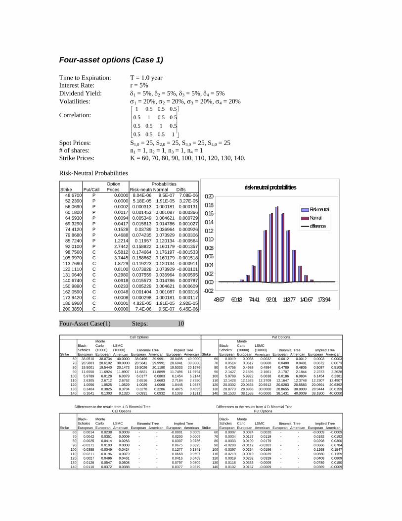
Four-asset options (Case 1) Time to Expiration: T = 1.0 year Interest Rate: r = 5% Dividend Yield: δ1 = 5%, δ2 = 5%, δ3 = 5%, δ4 = 5% Volatilities: σ1 = 20%, σ2 = 20%, σ3 = 20%, σ4 = 20%
Correlation:
⎥⎥⎥⎥
⎦
⎤
⎢⎢⎢⎢
⎣
⎡
15.05.05.05.015.05.05.05.015.05.05.05.01
Spot Prices: S1,0 = 25, S2,0 = 25, S3,0 = 25, S4,0 = 25 # of shares: n1 = 1, n2 = 1, n3 = 1, n4 = 1 Strike Prices: K = 60, 70, 80, 90, 100, 110, 120, 130, 140. Risk-Neutral Probabilities
OptionStrike Put/Call Prices Risk-neutraNormal Diffs
48.6700 P 0.0000 8.04E-06 9.5E-07 7.08E-0652.2390 P 0.0000 5.18E-05 1.91E-05 3.27E-0556.0690 P 0.0002 0.000313 0.000181 0.00013160.1800 P 0.0017 0.001453 0.001087 0.00036664.5930 P 0.0094 0.005349 0.004621 0.00072969.3290 P 0.0417 0.015813 0.014786 0.00102774.4120 P 0.1528 0.03789 0.036964 0.00092679.8680 P 0.4688 0.074235 0.073929 0.00030685.7240 P 1.2214 0.11957 0.120134 -0.00056492.0100 P 2.7442 0.158822 0.160179 -0.00135798.7560 C 6.5812 0.174664 0.176197 -0.001533
105.9970 C 3.7445 0.158662 0.160179 -0.001518113.7690 C 1.8729 0.119223 0.120134 -0.000911122.1110 C 0.8100 0.073828 0.073929 -0.000101131.0640 C 0.2980 0.037559 0.036964 0.000595140.6740 C 0.0918 0.015573 0.014786 0.000787150.9890 C 0.0233 0.005229 0.004621 0.000609162.0590 C 0.0048 0.001404 0.001087 0.000316173.9420 C 0.0008 0.000298 0.000181 0.000117186.6960 C 0.0001 4.82E-05 1.91E-05 2.92E-05200.3850 C 0.0000 7.4E-06 9.5E-07 6.45E-06
Probabilities risk-neutral probabilities
-0.020.000.020.040.060.080.100.120.140.160.180.20
48.67 60.18 74.41 92.01 113.77 140.67 173.94
Risk-neutralNormaldifference
Four-Asset Case(1) Steps: 10
Black-Scholes
Monte Carlo (10000)
LSMC (10000)
Black-Scholes
Monte Carlo (10000)
LSMC (10000)
Strike European European American European American European American Strike European European American European American European American60 38.0510 38.0734 40.0000 38.0496 39.9991 38.0495 40.0000 60 0.0019 0.0036 0.0032 0.0012 0.0012 0.0003 0.000370 28.5883 28.6192 30.0000 28.5841 29.9991 28.6041 30.0000 70 0.0514 0.0617 0.0600 0.0480 0.0481 0.0672 0.067380 19.5001 19.5440 20.1473 19.5026 20.1190 19.5333 20.1976 80 0.4756 0.4988 0.4984 0.4789 0.4805 0.5087 0.510590 11.6550 11.6924 11.8907 11.6821 11.8899 11.7496 11.9794 90 2.1427 2.1595 2.1661 2.1707 2.1844 2.2373 2.2628
100 5.9789 6.0128 6.0379 6.0177 6.0803 6.1454 6.2144 100 5.9789 5.9922 6.0638 6.0186 6.0834 6.1454 6.2381110 2.6305 2.6712 2.6762 2.6516 2.6683 2.7184 2.7380 110 12.1428 12.1628 12.3709 12.1647 12.3748 12.2307 12.4907120 1.0056 1.0525 1.0529 1.0029 1.0068 1.0445 1.0537 120 20.0302 20.0565 20.5912 20.0283 20.5583 20.0691 20.6392130 0.3404 0.3825 0.3794 0.3278 0.3286 0.4075 0.4095 130 28.8773 28.8988 30.0000 28.8655 30.0009 28.9444 30.0159140 0.1041 0.1303 0.1320 0.0931 0.0932 0.1308 0.1311 140 38.1533 38.1588 40.0000 38.1431 40.0009 38.1800 40.0000
Black-Scholes
Monte Carlo LSMC
Black-Scholes
Monte Carlo LSMC
Strike European European American European American European American Strike European European American European American European American60 0.0014 0.0238 0.0009 - - -0.0001 0.0009 60 0.0007 0.0024 0.0020 - - -0.0009 -0.000970 0.0042 0.0351 0.0009 - - 0.0200 0.0009 70 0.0034 0.0137 0.0119 - - 0.0192 0.019280 -0.0025 0.0414 0.0283 - - 0.0307 0.0786 80 -0.0033 0.0199 0.0179 - - 0.0298 0.030090 -0.0271 0.0103 0.0008 - - 0.0675 0.0895 90 -0.0280 -0.0112 -0.0183 - - 0.0666 0.0784
100 -0.0388 -0.0049 -0.0424 - - 0.1277 0.1341 100 -0.0397 -0.0264 -0.0196 - - 0.1268 0.1547110 -0.0211 0.0196 0.0079 - - 0.0668 0.0697 110 -0.0219 -0.0019 -0.0039 - - 0.0660 0.1159120 0.0027 0.0496 0.0461 - - 0.0416 0.0469 120 0.0019 0.0282 0.0329 - - 0.0408 0.0809130 0.0126 0.0547 0.0508 - - 0.0797 0.0809 130 0.0118 0.0333 -0.0009 - - 0.0789 0.0150140 0.0110 0.0372 0.0388 - - 0.0377 0.0379 140 0.0102 0.0157 -0.0009 - - 0.0369 -0.0009
Implied Tree
Differences to the results from 4-D Binomial Tree Differences to the results from 4-D Binomial TreeCall Options Put Options
Binomial Tree Implied Tree Binomial Tree
Call Options Put Options
Binomial Tree Implied Tree Binomial Tree Implied Tree

Four-Asset Case(1) Steps: 20
Black-Scholes
Monte Carlo (10000)
LSMC (10000)
Black-Scholes
Monte Carlo (10000)
LSMC (10000)
Strike European European American European American European American Strike European European American European American European American60 38.0510 38.0379 40.0000 38.0503 39.9996 38.0508 40.0000 60 0.0019 0.0010 0.0015 0.0016 0.0016 0.0016 0.001670 28.5883 28.5698 30.0000 28.5868 29.9996 28.5933 30.0000 70 0.0514 0.0452 0.0482 0.0503 0.0504 0.0564 0.056680 19.5003 19.4867 20.2131 19.5044 20.1320 19.5104 20.1545 80 0.4757 0.4743 0.4882 0.4803 0.4822 0.4858 0.489190 11.6553 11.6288 11.9001 11.6757 11.8884 11.7696 11.9948 90 2.1430 2.1287 2.1573 2.1639 2.1785 2.2573 2.2738
100 5.9793 5.9436 6.0146 6.0082 6.0737 6.0938 6.1637 100 5.9793 5.9559 6.0213 6.0086 6.0753 6.0938 6.1731110 2.6309 2.6097 2.6607 2.6497 2.6680 2.7805 2.8025 110 12.1431 12.1342 12.3805 12.1624 12.3757 12.2928 12.5150120 1.0058 1.0004 1.0327 1.0102 1.0149 1.0790 1.0858 120 20.0304 20.0372 20.5592 20.0352 20.5684 20.1036 20.6439130 0.3405 0.3270 0.3420 0.3374 0.3384 0.3589 0.3609 130 28.8774 28.8761 30.0000 28.8747 30.0004 28.8958 30.0068140 0.1042 0.0926 0.1020 0.1000 0.1003 0.1063 0.1068 140 38.1533 38.1540 40.0000 38.1496 40.0004 38.1555 40.0000
Black-Scholes
Monte Carlo LSMC
Black-Scholes
Monte Carlo LSMC
Strike European European American European American European American Strike European European American European American European American60 0.0007 -0.0124 0.0004 - - 0.0005 0.0004 60 0.0003 -0.0006 -0.0001 - - 0.0000 0.000070 0.0015 -0.0170 0.0004 - - 0.0065 0.0004 70 0.0011 -0.0051 -0.0022 - - 0.0061 0.006280 -0.0041 -0.0177 0.0811 - - 0.0060 0.0225 80 -0.0046 -0.0060 0.0060 - - 0.0055 0.006990 -0.0204 -0.0469 0.0117 - - 0.0939 0.1064 90 -0.0209 -0.0352 -0.0212 - - 0.0934 0.0953
100 -0.0289 -0.0646 -0.0591 - - 0.0856 0.0900 100 -0.0293 -0.0527 -0.0540 - - 0.0852 0.0978110 -0.0188 -0.0400 -0.0073 - - 0.1308 0.1345 110 -0.0193 -0.0282 0.0048 - - 0.1304 0.1393120 -0.0044 -0.0098 0.0178 - - 0.0688 0.0709 120 -0.0048 0.0020 -0.0092 - - 0.0684 0.0755130 0.0031 -0.0104 0.0036 - - 0.0215 0.0225 130 0.0027 0.0014 -0.0004 - - 0.0211 0.0064140 0.0042 -0.0074 0.0017 - - 0.0063 0.0065 140 0.0037 0.0044 -0.0004 - - 0.0059 -0.0004
Differences to the results from 4-D Binomial Tree
Implied Tree Binomial Tree Implied Tree
Put OptionsCall Options
Binomial Tree
Differences to the results from 4-D Binomial Tree
Call Options Put Options
Binomial Tree Implied Tree Binomial Tree Implied Tree
Four-Asset Case(1) Steps:4 100 20 steps are applied to the 4-Dimensional Binomial Tree, Monte Carlo simulation, and Least-squares Monte Carlo simulation. 100 steps are applied to the implied tree.
Black-Scholes
Monte Carlo (10000)
LSMC (10000)
Black-Scholes
Monte Carlo (10000)
LSMC (10000)
Strike European European American European American European American Strike European European American European American European American60 38.0510 38.0379 40.0000 38.0503 39.9996 38.0509 40.0000 60 0.0019 0.0010 0.0015 0.0016 0.0016 0.0017 0.001770 28.5883 28.5698 30.0000 28.5868 29.9996 28.5882 30.0000 70 0.0514 0.0452 0.0482 0.0503 0.0504 0.0513 0.051480 19.5003 19.4867 20.2131 19.5044 20.1320 19.5141 20.1461 80 0.4757 0.4743 0.4882 0.4803 0.4822 0.4895 0.491790 11.6553 11.6288 11.9001 11.6757 11.8884 11.6819 11.9012 90 2.1430 2.1287 2.1573 2.1639 2.1785 2.1696 2.1858
100 5.9793 5.9436 6.0146 6.0082 6.0737 6.0363 6.1047 100 5.9793 5.9559 6.0213 6.0086 6.0753 6.0363 6.1055110 2.6309 2.6097 2.6607 2.6497 2.6680 2.6748 2.6944 110 12.1431 12.1342 12.3805 12.1624 12.3757 12.1871 12.4040120 1.0058 1.0004 1.0327 1.0102 1.0149 1.0189 1.0240 120 20.0304 20.0372 20.5592 20.0352 20.5684 20.0435 20.5834130 0.3405 0.3270 0.3420 0.3374 0.3384 0.3452 0.3466 130 28.8774 28.8761 30.0000 28.8747 30.0004 28.8821 30.0085140 0.1042 0.0926 0.1020 0.1000 0.1003 0.1004 0.1007 140 38.1533 38.1540 40.0000 38.1496 40.0004 38.1496 40.0000
Black-Scholes
Monte Carlo LSMC
Black-Scholes
Monte Carlo LSMC
Strike European European American European American European American Strike European European American European American European American60 0.0007 -0.0124 0.0004 - - 0.0006 0.0004 60 0.0003 -0.0006 -0.0001 - - 0.0001 0.000170 0.0015 -0.0170 0.0004 - - 0.0014 0.0004 70 0.0011 -0.0051 -0.0022 - - 0.0010 0.001080 -0.0041 -0.0177 0.0811 - - 0.0097 0.0141 80 -0.0046 -0.0060 0.0060 - - 0.0092 0.009590 -0.0204 -0.0469 0.0117 - - 0.0062 0.0128 90 -0.0209 -0.0352 -0.0212 - - 0.0057 0.0073
100 -0.0289 -0.0646 -0.0591 - - 0.0281 0.0310 100 -0.0293 -0.0527 -0.0540 - - 0.0277 0.0302110 -0.0188 -0.0400 -0.0073 - - 0.0251 0.0264 110 -0.0193 -0.0282 0.0048 - - 0.0247 0.0283120 -0.0044 -0.0098 0.0178 - - 0.0087 0.0091 120 -0.0048 0.0020 -0.0092 - - 0.0083 0.0150130 0.0031 -0.0104 0.0036 - - 0.0078 0.0082 130 0.0027 0.0014 -0.0004 - - 0.0074 0.0081140 0.0042 -0.0074 0.0017 - - 0.0004 0.0004 140 0.0037 0.0044 -0.0004 - - 0.0000 -0.0004
Implied Tree Binomial Tree Implied TreeBinomial Tree
Binomial Tree Implied Tree Binomial Tree Implied Tree
Differences to the results from 4-D Binomial Tree Differences to the results from 4-D Binomial TreeCall Options Put Options
Call Options Put Options
4 20 steps are applied to the 4-Dimensional Binomial Tree, Monte Carlo simulation, and Least-squares Monte Carlo simulation. 100 steps are applied to the implied tree.
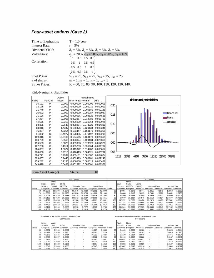
Four-asset options (Case 2) Time to Expiration: T = 1.0 year Interest Rate: r = 5% Dividend Yield: δ1 = 5%, δ2 = 5%, δ3 = 5%, δ4 = 5% Volatilities: σ1 = 20%, σ2 = 90%, σ3 = 90%, σ4 = 10%
Correlation:
⎥⎥⎥⎥
⎦
⎤
⎢⎢⎢⎢
⎣
⎡
15.05.05.05.015.05.05.05.015.05.05.05.01
Spot Prices: S1,0 = 25, S2,0 = 25, S3,0 = 25, S4,0 = 25 # of shares: n1 = 1, n2 = 1, n3 = 1, n4 = 1 Strike Prices: K = 60, 70, 80, 90, 100, 110, 120, 130, 140. Risk-Neutral Probabilities
OptionStrike Put/Call Prices Risk-neutraNormal Diffs
15.191 P 0.0000 0.000000 0.000001 -0.00000118.176 P 0.0000 0.000000 0.000019 -0.00001921.748 P 0.0000 0.000000 0.000181 -0.00018126.022 P 0.0000 0.000000 0.001087 -0.00108731.136 P 0.0000 0.000086 0.004621 -0.00453537.254 P 0.0005 0.002987 0.014786 -0.01179944.575 P 0.0219 0.026039 0.036964 -0.01092553.335 P 0.2645 0.088264 0.073929 0.01433563.816 P 1.4347 0.158476 0.120134 0.03834176.357 P 4.7254 0.183447 0.160179 0.02326891.362 C 19.4977 0.178405 0.176197 0.002208
109.316 C 13.3103 0.134565 0.160179 -0.025615130.799 C 8.6566 0.093824 0.120134 -0.026310156.503 C 5.3825 0.059003 0.073929 -0.014926187.258 C 3.1911 0.035233 0.036964 -0.001732224.057 C 1.8024 0.019842 0.014786 0.005057268.088 C 0.9718 0.010413 0.004621 0.005792320.771 C 0.4999 0.005161 0.001087 0.004074383.807 C 0.2446 0.002429 0.000181 0.002248459.232 C 0.1135 0.000506 0.000019 0.000487549.478 C 0.0498 0.001322 0.000001 0.001321
Probabilitiesrisk-neutral probabilities
-0.05
0.00
0.05
0.10
0.15
0.20
15.19 26.02 44.58 76.36 130.80 224.06 383.81
Risk-neutralNormaldifference
Four-Asset Case(2) Steps: 10
Black-Scholes
Monte Carlo (10000)
LSMC (10000)
Black-Scholes
Monte Carlo (10000)
LSMC (10000)
Strike European European American European American European American Strike European European American European American European American60 39.3576 39.1209 40.3079 38.7645 40.0220 39.2532 40.3900 60 1.3084 0.8678 0.8774 0.8615 0.8648 1.2040 1.209270 31.6036 31.5524 32.0958 31.1838 31.8708 31.4220 32.1934 70 3.0668 2.8115 2.8295 2.7931 2.8088 2.8851 2.895880 24.9045 25.3539 25.7533 24.9724 25.3769 25.6936 26.1593 80 5.8800 6.1253 6.1450 6.0939 6.1401 6.6690 6.720590 19.3193 20.4029 20.6683 20.0172 20.2687 20.1800 20.5651 90 9.8070 10.6867 10.7546 10.6510 10.7524 10.6677 10.7665
100 14.7972 16.4895 16.7674 16.1168 16.2794 16.7031 16.9341 100 14.7972 16.2856 16.4456 16.2629 16.4483 16.7031 16.9224110 11.2208 13.4208 13.6958 13.0248 13.1354 13.5482 13.7432 110 20.7331 22.7292 22.9688 22.6832 22.9911 23.0605 23.3799120 8.4436 10.9813 11.2089 10.6211 10.6967 10.7565 10.8817 120 27.4682 29.8019 30.0989 29.7918 30.2518 29.7811 30.3875130 6.3172 9.0364 9.2077 8.6718 8.7272 9.1763 9.2760 130 34.8541 37.3693 37.7925 37.3548 38.0141 37.7132 38.5033140 4.7067 7.4896 7.5673 7.1528 7.1913 7.5961 7.6776 140 42.7558 45.3348 45.9888 45.3481 46.2362 45.6452 46.7075
Black-Scholes
Monte Carlo LSMC
Black-Scholes
Monte Carlo LSMC
Strike European European American European American European American Strike European European American European American European American60 0.5931 0.3564 0.2859 - - 0.4887 0.3680 60 0.4469 0.0063 0.0126 - - 0.3425 0.344470 0.4198 0.3686 0.2250 - - 0.2382 0.3226 70 0.2737 0.0184 0.0207 - - 0.0920 0.087080 -0.0679 0.3815 0.3764 - - 0.7212 0.7824 80 -0.2139 0.0314 0.0049 - - 0.5751 0.580490 -0.6979 0.3857 0.3996 - - 0.1628 0.2964 90 -0.8440 0.0357 0.0022 - - 0.0167 0.0141
100 -1.3196 0.3727 0.4880 - - 0.5863 0.6547 100 -1.4657 0.0227 -0.0027 - - 0.4402 0.4741110 -1.8040 0.3960 0.5604 - - 0.5234 0.6078 110 -1.9501 0.0460 -0.0223 - - 0.3773 0.3888120 -2.1775 0.3602 0.5122 - - 0.1354 0.1850 120 -2.3236 0.0101 -0.1529 - - -0.0107 0.1357130 -2.3546 0.3646 0.4805 - - 0.5045 0.5488 130 -2.5007 0.0145 -0.2216 - - 0.3584 0.4892140 -2.4461 0.3368 0.3760 - - 0.4433 0.4863 140 -2.5923 -0.0133 -0.2474 - - 0.2971 0.4713
Implied Tree Binomial Tree Implied Tree
Differences to the results from 4-D Binomial Tree Differences to the results from 4-D Binomial TreeCall Options Put Options
Binomial Tree
Call Options Put Options
Binomial Tree Implied Tree Binomial Tree Implied Tree

Four-Asset Case(2) Steps: 20
Black-Scholes
Monte Carlo (10000)
LSMC (10000)
Black-Scholes
Monte Carlo (10000)
LSMC (10000)
Strike European European American European American European American Strike European European American European American European American60 39.3672 38.7803 40.3251 38.8348 40.1233 39.0578 40.2466 60 1.3180 0.8521 0.8627 0.8593 0.8629 1.0086 1.011670 31.6195 31.1542 32.1446 31.2476 31.9577 31.5943 32.2983 70 3.0826 2.7383 2.7676 2.7844 2.8009 3.0574 3.072080 24.9262 24.9224 25.6184 25.0341 25.4568 25.3417 25.8114 80 5.9016 6.0187 6.0873 6.0831 6.1303 6.3171 6.364990 19.3452 19.9858 20.4219 20.0855 20.3525 20.1984 20.5528 90 9.8329 10.5944 10.7683 10.6469 10.7497 10.6861 10.7806
100 14.8255 16.1194 16.3547 16.1867 16.3632 16.5209 16.7634 100 14.8255 16.2403 16.4739 16.2604 16.4492 16.5209 16.7100110 11.2496 13.1004 13.1441 13.1225 13.2435 13.1622 13.3470 110 20.7619 22.7336 23.0882 22.7084 23.0167 22.6744 23.0341120 8.4713 10.7234 10.8402 10.7092 10.7946 10.9959 11.1348 120 27.4959 29.8689 30.3944 29.8074 30.2716 30.0205 30.5325130 6.3429 8.8651 8.8757 8.7906 8.8524 8.8296 8.9450 130 34.8798 37.5229 38.2540 37.4011 38.0604 37.3665 38.1477140 4.7296 7.4124 7.5243 7.2697 7.3154 7.4846 7.5669 140 42.7788 45.5825 46.5738 45.3925 46.2834 45.5338 46.5786
Black-Scholes
Monte Carlo LSMC
Black-Scholes
Monte Carlo LSMC
Strike European European American European American European American Strike European European American European American European American60 0.5324 -0.0545 0.2018 - - 0.2230 0.1233 60 0.4587 -0.0072 -0.0002 - - 0.1493 0.148770 0.3719 -0.0934 0.1869 - - 0.3467 0.3406 70 0.2982 -0.0461 -0.0333 - - 0.2730 0.271180 -0.1079 -0.1117 0.1616 - - 0.3076 0.3546 80 -0.1815 -0.0644 -0.0430 - - 0.2340 0.234690 -0.7403 -0.0997 0.0694 - - 0.1129 0.2003 90 -0.8140 -0.0525 0.0186 - - 0.0392 0.0309
100 -1.3612 -0.0673 -0.0085 - - 0.3342 0.4002 100 -1.4349 -0.0201 0.0247 - - 0.2605 0.2608110 -1.8729 -0.0221 -0.0994 - - 0.0397 0.1035 110 -1.9465 0.0252 0.0715 - - -0.0340 0.0174120 -2.2379 0.0142 0.0456 - - 0.2867 0.3402 120 -2.3115 0.0615 0.1228 - - 0.2131 0.2609130 -2.4477 0.0745 0.0233 - - 0.0390 0.0926 130 -2.5213 0.1218 0.1936 - - -0.0346 0.0873140 -2.5401 0.1427 0.2089 - - 0.2149 0.2515 140 -2.6137 0.1900 0.2904 - - 0.1413 0.2952
Differences to the results from 4-D Binomial Tree Differences to the results from 4-D Binomial TreeCall Options Put Options
Binomial Tree Implied Tree Binomial Tree Implied Tree
Call Options Put Options
Binomial Tree Implied Tree Binomial Tree Implied Tree
Four-Asset Case(2) Steps:5 100
Black-Scholes
Monte Carlo (10000)
LSMC (10000)
Black-Scholes
Monte Carlo (10000)
LSMC (10000)
Strike European European American European American European American Strike European European American European American European American60 39.3672 38.7803 40.3251 38.8348 40.1233 38.9332 40.1687 60 1.3180 0.8521 0.8627 0.8593 0.8629 0.8840 0.885870 31.6195 31.1542 32.1446 31.2476 31.9577 31.3686 32.0787 70 3.0826 2.7383 2.7676 2.7844 2.8009 2.8317 2.841880 24.9262 24.9224 25.6184 25.0341 25.4568 25.1671 25.6338 80 5.9016 6.0187 6.0873 6.0831 6.1303 6.1425 6.177890 19.3452 19.9858 20.4219 20.0855 20.3525 20.1417 20.4732 90 9.8329 10.5944 10.7683 10.6469 10.7497 10.6294 10.7154
100 14.8255 16.1194 16.3547 16.1867 16.3632 16.2154 16.4545 100 14.8255 16.2403 16.4739 16.2604 16.4492 16.2154 16.3953110 11.2496 13.1004 13.1441 13.1225 13.2435 13.1775 13.3555 110 20.7619 22.7336 23.0882 22.7084 23.0167 22.6898 23.0026120 8.4713 10.7234 10.8402 10.7092 10.7946 10.7623 10.8979 120 27.4959 29.8689 30.3944 29.8074 30.2716 29.7869 30.2822130 6.3429 8.8651 8.8757 8.7906 8.8524 8.8436 8.9487 130 34.8798 37.5229 38.2540 37.4011 38.0604 37.3805 38.1080140 4.7296 7.4124 7.5243 7.2697 7.3154 7.3094 7.3920 140 42.7788 45.5825 46.5738 45.3925 46.2834 45.3586 46.3657
Black-Scholes
Monte Carlo LSMC
Black-Scholes
Monte Carlo LSMC
Strike European European American European American European American Strike European European American European American European American60 0.5324 -0.0545 0.2018 - - 0.0984 0.0454 60 0.4587 -0.0072 -0.0002 - - 0.0247 0.022970 0.3719 -0.0934 0.1869 - - 0.1210 0.1210 70 0.2982 -0.0461 -0.0333 - - 0.0473 0.040980 -0.1079 -0.1117 0.1616 - - 0.1330 0.1770 80 -0.1815 -0.0644 -0.0430 - - 0.0594 0.047590 -0.7403 -0.0997 0.0694 - - 0.0562 0.1207 90 -0.8140 -0.0525 0.0186 - - -0.0175 -0.0343
100 -1.3612 -0.0673 -0.0085 - - 0.0287 0.0913 100 -1.4349 -0.0201 0.0247 - - -0.0450 -0.0539110 -1.8729 -0.0221 -0.0994 - - 0.0550 0.1120 110 -1.9465 0.0252 0.0715 - - -0.0186 -0.0141120 -2.2379 0.0142 0.0456 - - 0.0531 0.1033 120 -2.3115 0.0615 0.1228 - - -0.0205 0.0106130 -2.4477 0.0745 0.0233 - - 0.0530 0.0963 130 -2.5213 0.1218 0.1936 - - -0.0206 0.0476140 -2.5401 0.1427 0.2089 - - 0.0397 0.0766 140 -2.6137 0.1900 0.2904 - - -0.0339 0.0823
Implied Tree Binomial Tree Implied Tree
Differences to the results from 4-D Binomial TreeDifferences to the results from 4-D Binomial TreeCall Options Put Options
Call Options Put Options
Binomial Tree
Binomial Tree Implied Tree Binomial Tree Implied Tree
5 20 steps are applied to the 4-Dimensional Binomial Tree, Monte Carlo simulation, and Least-squares Monte Carlo simulation. 100 steps are applied to the implied tree.

Appendix A:
Valuing American-style options using binomial trees
Univariate Binomial Tree Cox, Ross and Rubinstein (1979) developed the binomial option pricing model which converges to the Black-Scholes formula in the continuous limit and demonstrates the advantage in valuing American-style options. The model approximates the behavior of an asset price by the upward and downward changes in the asset price over a particular interval of time.
SudS
u2S
dS
uS
d2Sd3S
ud2S
u2dS
u3S
d4S
ud3S
u2d2S
u3dS
u4S
As shown in Figure 1, an asset with a current price of S follows a multiplicative binomial process in which the asset price can either go up to uS or down to dS, during the interval h = T/m, where m is the total number of moves over time. The figure 1 demonstrates a four moves binomial tree. Cox, Ross and Rubinstein (1979) has shown that the upward and downward movements, i.e., u and d, can be chosen such that the probabilities of each movements to be equally one-half. In addition, the mean and variance of the discrete binomial process matches those of the risk-neutral process of the asset price over the time step of the binomial tree. The structure leads to:
( ) ( )
mThdrv
phvhdhvhu
/
expexp
221
21
≡
−−≡
=−=+=
σ
σσ
After constructing the tree of asset prices, the valuation of options can be worked backwards by applying the concept that the value of a security is its risk-neutral expectation of discounted payoffs. In our setup, since both up and down moves have the equal probability of one-half, the holding value of security is the discounted average of its value in the next interval. If it is an American-style option, the value of the option at a particular time, is its intrinsic value or the holding value, whichever is greater. Consider an American put option with two moves, m =2, for example. At expiration, depending on the asset prices, the value of option will be: C(u2S) = max 0, K – u2S C(udS) = max 0, K – udS

C(d2S) = max 0, K – d2S Working backwards by one move, we have, C(uS) = max K – uS, ½[C(u2S) + C(udS)] * log(-r*h) C(dS) = max K – dS, ½[C(udS) + C(d2S)] * log(-r*h) And, finally, working backwards one more move to the beginning of the tree: C(S) = max K – S, ½[C(uS) + C(dS)] * log(-r*h)
Bivariate Binomial Tree Rubinstein (1995) shows an approach to value options with two underlying assets by approximating continuous bivariate normal density function with a discrete bivariate binomial density. The structure, or called "binomial pyramids", is shown in Figure 1.
(1, 1)
(d, D)(d, C)
(u, A) (u, B)
¼¼
¼¼
Move 1
(d, D)(d, C)
(u, A) (u, B)
¼¼
¼¼
(ud, BC)=
(du, AD)
(d2, D2)(d2, CD)(d2, C2)
(du, BD)(ud, AC)
(u2, B2)(u2, A2) (u2, AB)
Move 2 The returns of the two underlying assets are written in pairs, and they start from (1, 1) at the beginning. During the first move, the first asset return is assumed to be either u or d, with equal probability. Simultaneously, if the first asset moves up by u, the second asset return may be either A or B with equal probability, depending on the correlation between two assets. Or, if the first asset moves down by d, the second asset return may be C or D. It structures total four possible outcomes, which are (u,A), (u,B), (d,C) and (d,D), with equal probability 1/4, which emanated from the pair (1,1). Figure 1 also shows the nodes after the second move. The multiplicative returns over two moves will be (u2, A2), (u2, AB), (ud, AC) and (ud, AD), if the return of first move was (u,A). The value of moves can be obtained as following:
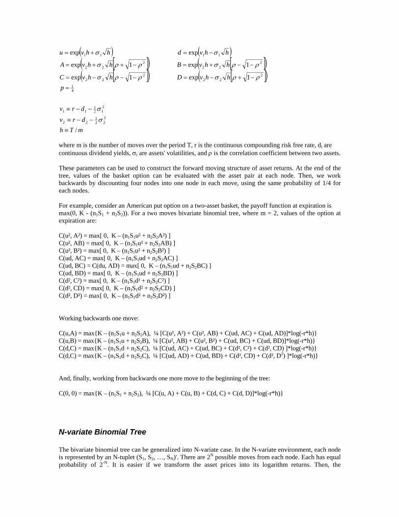
( ) ( )[ ]( ) [ ]( )[ ]( ) [ ]( )
mThdrv
drv
phhvDhhvC
hhvBhhvA
hhvdhhvu
/
1exp1exp
1exp1exp
expexp
222
122
212
111
41
222
222
222
222
1111
≡
−−≡
−−≡
=
−+−=−−−=
−−+=−++=
−=+=
σ
σ
ρρσρρσ
ρρσρρσ
σσ
where m is the number of moves over the period T, r is the continuous compounding risk free rate, di are continuous dividend yields, σi are assets' volatilities, and ρ is the correlation coefficient between two assets. These parameters can be used to construct the forward moving structure of asset returns. At the end of the tree, values of the basket option can be evaluated with the asset pair at each node. Then, we work backwards by discounting four nodes into one node in each move, using the same probability of 1/4 for each nodes. For example, consider an American put option on a two-asset basket, the payoff function at expiration is max(0, K - (n1S1 + n2S2)). For a two moves bivariate binomial tree, where m = 2, values of the option at expiration are: C(u², A²) = max[ 0, K – (n1S1u² + n2S2A²) ] C(u², AB) = max[ 0, K – (n1S1u² + n2S2AB) ] C(u², B²) = max[ 0, K – (n1S1u² + n2S2B²) ] C(ud, AC) = max[ 0, K – (n1S1ud + n2S2AC) ] C(ud, BC) = C(du, AD) = max[ 0, K – (n1S1ud + n2S2BC) ] C(ud, BD) = max[ 0, K – (n1S1ud + n2S2BD) ] C(d², C²) = max[ 0, K – (n1S1d² + n2S2C²) ] C(d², CD) = max[ 0, K – (n1S1d² + n2S2CD) ] C(d², D²) = max[ 0, K – (n1S1d² + n2S2D²) ] Working backwards one move: C(u,A) = maxK – (n1S1u + n2S2A), ¼ [C(u², A²) + C(u², AB) + C(ud, AC) + C(ud, AD)]*log(-r*h) C(u,B) = maxK – (n1S1u + n2S2B), ¼ [C(u², AB) + C(u², B²) + C(ud, BC) + C(ud, BD)]*log(-r*h) C(d,C) = maxK – (n1S1d + n2S2C), ¼ [C(ud, AC) + C(ud, BC) + C(d², C²) + C(d², CD) ]*log(-r*h) C(d,C) = maxK – (n1S1d + n2S2C), ¼ [C(ud, AD) + C(ud, BD) + C(d², CD) + C(d², D2) ]*log(-r*h) And, finally, working from backwards one more move to the beginning of the tree: C(0, 0) = maxK – (n1S1 + n2S2), ¼ [C(u, A) + C(u, B) + C(d, C) + C(d, D)]*log(-r*h)
N-variate Binomial Tree The bivariate binomial tree can be generalized into N-variate case. In the N-variate environment, each node is represented by an N-tuplet (S1, S2, …, SN)'. There are 2N possible moves from each node. Each has equal probability of 2-N. It is easier if we transform the asset prices into its logarithm returns. Then, the
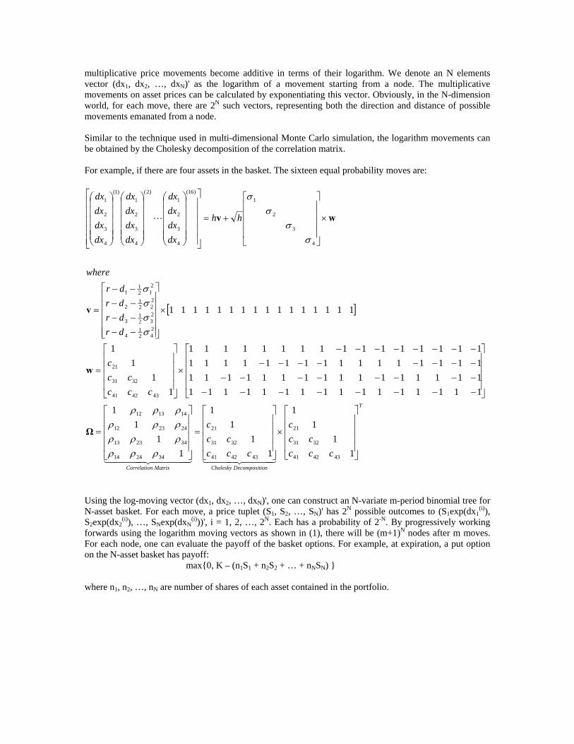
multiplicative price movements become additive in terms of their logarithm. We denote an N elements vector (dx1, dx2, …, dxN)' as the logarithm of a movement starting from a node. The multiplicative movements on asset prices can be calculated by exponentiating this vector. Obviously, in the N-dimension world, for each move, there are 2N such vectors, representing both the direction and distance of possible movements emanated from a node. Similar to the technique used in multi-dimensional Monte Carlo simulation, the logarithm movements can be obtained by the Cholesky decomposition of the correlation matrix. For example, if there are four assets in the basket. The sixteen equal probability moves are:
[ ]
T
ionDecompositCholeskyMatrixnCorrelatio
ccccc
c
ccccc
c
ccccc
c
drdrdrdr
where
hh
dxdxdxdx
dxdxdxdx
dxdxdxdx
⎥⎥⎥⎥
⎦
⎤
⎢⎢⎢⎢
⎣
⎡
×
⎥⎥⎥⎥
⎦
⎤
⎢⎢⎢⎢
⎣
⎡
=
⎥⎥⎥⎥
⎦
⎤
⎢⎢⎢⎢
⎣
⎡
=
⎥⎥⎥⎥
⎦
⎤
⎢⎢⎢⎢
⎣
⎡
−−−−−−−−−−−−−−−−−−−−−−−−−−−−−−−−
×
⎥⎥⎥⎥
⎦
⎤
⎢⎢⎢⎢
⎣
⎡
=
×
⎥⎥⎥⎥⎥
⎦
⎤
⎢⎢⎢⎢⎢
⎣
⎡
−−−−−−−−
=
×
⎥⎥⎥⎥
⎦
⎤
⎢⎢⎢⎢
⎣
⎡
+=
⎥⎥⎥⎥⎥
⎦
⎤
⎢⎢⎢⎢⎢
⎣
⎡
⎟⎟⎟⎟⎟
⎠
⎞
⎜⎜⎜⎜⎜
⎝
⎛
⎟⎟⎟⎟⎟
⎠
⎞
⎜⎜⎜⎜⎜
⎝
⎛
⎟⎟⎟⎟⎟
⎠
⎞
⎜⎜⎜⎜⎜
⎝
⎛
11
11
11
11
11
11
1111111111111111111111111111111111111111111111111111111111111111
11
11
1111111111111111
434241
3231
21
434241
3231
21
342414
342313
242312
141312
434241
3231
21
242
14
232
13
222
12
212
11
4
3
2
1)16(
4
3
2
1)2(
4
3
2
1)1(
4
3
2
1
444 3444 214444 34444 21
L
ρρρρρρρρρρρρ
σσσσ
σσ
σσ
Ω
w
v
wv
Using the log-moving vector (dx1, dx2, …, dxN)', one can construct an N-variate m-period binomial tree for N-asset basket. For each move, a price tuplet (S1, S2, …, SN)' has 2N possible outcomes to (S1exp(dx1
(i)), S2exp(dx2
(i)), …, SNexp(dxN(i)))', i = 1, 2, …, 2N. Each has a probability of 2-N. By progressively working
forwards using the logarithm moving vectors as shown in (1), there will be (m+1)N nodes after m moves. For each node, one can evaluate the payoff of the basket options. For example, at expiration, a put option on the N-asset basket has payoff:
max0, K – (n1S1 + n2S2 + … + nNSN)
where n1, n2, …, nN are number of shares of each asset contained in the portfolio.

Appendix B:
Valuing European-style multi-asset basket options using Monte Carlo simulation Assuming all the underlying assets of a basket option follows geometric Brownian motion (GBM) processes.
( )( )
( ) NNNNNN dwSdtSdrdS
dwSdtSdrdSdwSdtSdrdS
σ
σσ
+−=
+−=+−=
M
222222
111111
where r is the continuous compounding risk-less interest rate, di's are dividend yield for each asset, σi's are return volatilities, and the two assets (i and j) have correlation ρij, i.e., dwidwj=ρijdt. The best way to simulate a GBM process is through a transformation to the natural logarithm of asset prices. Let xi = ln(Si), via Ito's Lemma, we have,
NNNN dwdtvdx
dwdtvdxdwdtvdx
σ
σσ
+=
+=+=
M2222
1111
where vi = r - di - σi
2/2. Next, we transform to a space where variables are uncorrelated. This can be conducted by decomposing the covariance matrix of original GBM process into its eigenvalues and eigenvectors.
444444 3444444 21
OM
L
O
444 3444 21
O
4444 34444 21
ML
MM
rixariancemat
NNN
N
N
NNNN
N
N
seigenvalue
N
rseigenvecto
NN
N
N
NN eee
eeeeee
e
ee
e
ee
e
ee
cov
221
22212
12121
21
22221
11211
2
1
2
1
2
22
21
1
12
11
⎥⎥⎥⎥⎥
⎦
⎤
⎢⎢⎢⎢⎢
⎣
⎡
=
⎥⎥⎥⎥
⎦
⎤
⎢⎢⎢⎢
⎣
⎡
⎥⎥⎥⎥
⎦
⎤
⎢⎢⎢⎢
⎣
⎡
⎥⎥⎥⎥⎥
⎦
⎤
⎢⎢⎢⎢⎢
⎣
⎡
⎟⎟⎟⎟⎟
⎠
⎞
⎜⎜⎜⎜⎜
⎝
⎛
⎟⎟⎟⎟⎟
⎠
⎞
⎜⎜⎜⎜⎜
⎝
⎛
⎟⎟⎟⎟⎟
⎠
⎞
⎜⎜⎜⎜⎜
⎝
⎛
σσρσσρσ
σρσσσρσσρσσρσσ
λ
λλ
The eigenvectors lead the linear combination of x1, x2, …, and xN be uncorrelated:
NNNNN
NN
NNNNN xexexe
xexexe
y
ywhere
dzdt
dzdt
dy
dy
+++
+++
=
=
+
+
=
=
L
L
MM
2211
121211111111
λα
λα

where αi = ei1v1+ei2v2+…+eiNvN, for all i = 1, …, N, and dzi, dzj are uncorrelated Brownian motions. Now, we can discretise the N uncorrelated arithmetic Brownian motions by replacing the infinitesimals dyi, dt and dzI with small changes Δyi, h, and random samples of εi√h. Those εi's are independent draws from standard normal distributions. h = T/m is the time step, m is the number of time periods over which we want to simulate. If we have ti = i h, i = 1, …,m, then the processes of yi's can be simulated by the following:
hhy
hhy
y
y
NiNNtN
it
tN
t
i
i
i
i
λεα
λεα
,,
1,11,1
,
,1
1
1
++
++
=
=
−
−
M
The asset prices at each time interval can be obtained by transforming the yi's back:
( ) NjxS
yeyeye
yeyeye
x
x
ii
iii
iii
i
i
tjtj
tNNNtNtN
tNNtt
tN
t
,,1exp ,,
,,22,11
,1,221,111
,
,1
L
L
L
M
=∀=⇒
+++
+++
=
=
where Sj,ti is the price of the j-th asset at the end of the i-th period. At the end of maturity, the payoffs of a European-style option can be determined by knowing the underlying asset prices from the simulation. If we repeat the process, and simulate large number of outcomes of asset prices at maturity, the value of the European-style option at time zero, can be estimated unbiasedly through its average of all the discounted payoff outcomes.
( )∑=
−=M
s
sTPayoffrT
MC
1
)(exp1ˆ
where M is the total number of simulations, and it is typically a large number where 10,000 is not unusual in practice, PayoffT
(s) is the option's payoff at maturity T under s-th simulation path. Consider a European-style put option on an N-asset basket. After the s-th simulation, the underlying asset prices become S1,T
(s), S2,T(s), …, SN,T
(s) at time T. Therefore, the payoff of the basket option is:
PayoffT(s) = max 0, K – [n1S1,T
(s) + n2S2,T(s) + … + nNSN,T
(s)]

References Andersen, L., and M. Broadie, 2001, "A Primal-Dual Simulation Algorithm for Pricing Multi-Dimensional American Options", Working paper, Columbia University. Barraquand, J., and D. Martineau, 1995, "Numerical Valuation of High Dimensional Multivariate American Securities", The Journal of Financial and Quantitative Analysis, Vol. 30, Issue 3, 1995, 383-405. Boyle, P., M. Broadie, and P. Glasserman, 1997, "Monte Carlo Methods for Security Pricing", Journal of Economic Dynamics and Control, 1997, Vol. 21. Nos. 8-9, 1267-1322. Breeden, D., and R. Litzenberger, 1978, "Prices of State-Contingent Claims Implicit in Options Prices", Journal of Business, 51, 1978, 621-651. Broadie, M., and J. Detemple, 1996, "American Option Valuation: New Bounds, Approximations, and a Comparison of Existing Methods", Review of Financial Studies, Vol. 9, Issue 4 (Winter 1996), 1211-1250. Broadie, M., and P. Glasserman, 1997, "A Stochastic Mesh Method for Pricing High-Dimensional American Options", working paper, Columbia PaineWebber Working Paper Series in Money, Economics and Finance. Broadie, M., and P. Glasserman, 1997a, "Pricing American-Style Securities Using Simulaion", Journal of Economic Dynamics and Control, 1997, Vol. 21, Nos. 8-9, 1323-1352. Broadie, M., and P. Glasserman, 1997b, "Monte Carlo Methods for Pricing High-Dimensional American Options: An Overview", Net Exposure: The Electronic Journal of Financial Risk, 1997, issue 3 (December) 15-37. Clewlow, L., and C. Strickland, 1998, "Implementing Derivatives Models", John Wiley & Sons, 1998. Cox, J., S. Ross, and M. Rubinstein, 1979, "Option Pricing: A Simplified Approach", Journal of Financial Economics, 7, No. 3, 1979, 229-263. Hull, J., 1997, "Options, Futures, and Other Derivatives", third edition, Prentice Hall, 1997, 361-364. Jackwerth, J., and M. Rubinstein, 1996, "Recovering Probability Distributions from Option Prices", Journal of Finance, 51, 1996, 1611-1631. Jackwerth, J., 1999, "Option-Implied Risk-Neutral Distributions and Implied Binomial Trees: A Literature Review", Journal of Derivatives, 7, No. 2, 66-82. Longstaff, F. and Schwartz, E., 2001, "Valuing American Options by Simulation: A Simple Least-Squares Approach", Review of Financial Studies, 14(1), Spring 2001, 113-147. Rubinstein, M., 1994, "Implied Binomial Trees", Journal of Finance, 49, No.3, 1994, 771-818. Rubinstein, M., 1994a, "Rainbow Options", Risk 7, November 1994, 67-71. Rubinstein, M., 1998, "Edgeworth Binomial Trees", Journal of Derivatives, 5, No.3, 1998, 20-27. Tilley, J., 1993, "Valuing American Options in a Path Simulation Model", Transactions of the Society of Actuaries, 45, 1993, 83-104. Wilmott, P., 1998, "The Theory and Practice of Financial Engineering", John Wiley & Sons, ISBN: 0471983896, 1998, 151-161.
Related Documents