Price Regulation and Environmental Externalities: Evidence .... Hausman... · Price Regulation and Environmental Externalities: Evidence ... man, Sarah Jacobson, Corey Lang, John

Price Regulation and Environmental Externalities: Evidence

from Methane Leaks

Catherine Hausman Lucija Muehlenbachs∗

January 2017

Abstract

We estimate how much US natural gas distribution firms spend to reduce methaneleaks. Methane is a significant contributor to climate change, so the wedge betweenthe private and social benefits of abatement is large. Moreover, incentives to abateleaks are additionally weakened by this industry being a regulated natural monopoly:current price regulations allow many distribution firms to pass the cost of any lost gason to their customers. Our estimates imply that too little is spent repairing leaks.In contrast, accelerated pipeline replacement cannot in general be justified by climatebenefits alone.

Key Words: natural gas, methane leaks, price regulation, utilities, pipelines, infrastructureJEL: Q41, L95, D22, D42

∗(Hausman) Ford School of Public Policy, University of Michigan; and National Bureau of EconomicsResearch. Email: [email protected]. (Muehlenbachs) Department of Economics, University of Calgary;and Resources for the Future. Email: [email protected]. We thank Kathy Baylis, Carl Blumstein,Severin Borenstein, Duncan Callaway, Lucas Davis, Rebecca Dell, Laura Grant, Sumeet Gulati, Josh Haus-man, Sarah Jacobson, Corey Lang, John Leahy, Erich Muehlegger, Jim Sallee, Stefan Staubli, Rich Sweeney,Justin Wolfers, Catherine Wolfram, seminar participants at Carnegie Mellon, Cornell, Duke-NCSU-RTI,EDF, UC-Davis, and participants at the NBER Future of Energy Distribution meeting, the Association ofEnvironmental and Resource Economics meeting, the Midwest Energy Fest, and the ASSA meetings forhelpful feedback. We are grateful to the Alfred P. Sloan Foundation, the Social Sciences and HumanitiesResearch Council of Canada, and Resource for the Future for financial support. All errors are our own.

Methane (CH4) emissions have been the focus of much recent public attention. This

invisible gas is 34 times more potent a greenhouse gas than carbon dioxide, yet its release to

the atmosphere has been largely unregulated. One source of methane emissions is leaks from

the natural gas industry: methane is the primary component of natural gas. Leaks through-

out the US natural gas supply chain result in roughly $8 billion dollars of climate impacts

annually.1 The US federal government is now developing standards to reduce methane leaks

in the oil and gas sector. However, the economics literature on methane leaks is largely

nonexistent. In this paper, we analyze leak abatement incentives at the natural gas distri-

bution firms that deliver gas to end-user customers. This is a sector that is not covered by

recent federal methane regulations, and it has had limited emissions reductions to date.2 The

academic literature that does exist has come primarily from engineers and natural scientists,

and it has emphasized measurement issues (Miller et al., 2013; Phillips et al., 2013; Brandt

et al., 2014; Howarth, 2014; Jackson et al., 2014a,b; Lamb et al., 2015; McKain et al., 2015).3

In contrast, we examine the financial incentives of firms to abate leaks. We are the first

in the economics literature to take advantage of data long-reported to the US government

on leaks from natural gas distribution companies. This is a contribution in its own right.

Some analysts have shied away from these data because of measurement error (Kirchgessner

et al., 1997; ICF International, 2014), however we provide empirical strategies that address

the data quality issues.

Leaks can occur from faulty connections, decaying infrastructure, or intentional venting

at every stage of the supply chain: extraction, storage, transmission, and distribution. We

1This calculation uses the 322 billion cubic feet (Bcf) the Environmental Protection Agency estimatedfor 2012 (DOE 2015), the most recent year for which data are finalized. For the social cost, we use a globalwarming potential of 34 and the Interagency Working Group’s social cost of carbon for 2015 emissions, $41per ton. Below we discuss this approach relative to using Marten et al. (2015)’s estimates of the social costof methane.

2See the May 2016 final rule to reduce methane from the oil and natural gas industry,https://www.epa.gov/stationary-sources-air-pollution/epas-actions-reduce-methane-and-volatile-organic-compound-voc.

3White papers and non-academic reports on methane leaks and aging pipelines include Aubuchon andHibbard, 2013; Costello, 2012; Costello, 2013; Department of Energy, 2015; Yardley Associates, 2012; ICFInternational, 2014; Webb, 2015.

1

focus on the distribution network; around 1,500 local distribution companies are responsible

for delivering natural gas to end users in residences and businesses. Distribution is a natural

monopoly because the necessary pipelines entail both large fixed costs and economies of

density (Joskow, 2007). As such, most natural gas distribution firms are price-regulated

investor-owned utilities. By regulating prices, inefficiencies are introduced, largely stemming

from the regulator’s inability to perfectly observe firm effort (Posner, 1969; Laffont and

Tirole, 1986; Joskow, 2007). We examine a previously unstudied distortion in the natural gas

distribution sector, in which firms are allowed to pass the cost of lost gas on to customers.

Leaked gas is treated as a cost of doing business; a 1935 Supreme Court decision stated

that “a certain loss [of natural gas] is unavoidable, no matter how carefully business is

conducted.”4 We are able to observe how much the investor-owned utilities spend each

period, as well as how much gas is leaked. We obtain an estimate of the cost that utilities

undertake to reduce leaks and compare it to value of the lost commodity (the price the

utility paid for the gas). The natural gas industry provides an excellent opportunity to test

the general question of whether price-regulated firms cost-minimize, because the researcher

is able to observe the commodity value of gas lost as well as effort undertaken to prevent

those losses.

Importantly, the distortion induced by price regulation in this setting is more costly

than in many other settings, because the leaked commodity imposes outsized external costs.

The full social cost of leaked natural gas is around an order of magnitude larger than the

commodity value.5 In contrast, the ratio of social to private cost is a little less than three

for combusted coal and less than two for combusted gasoline (Parry et al., 2014). Thus in

a second-best setting without a carbon tax, reducing distortions stemming from economic

regulations could have substantial environmental benefits. Additionally, given the rapid

recent growth in the natural gas market (Hausman and Kellogg, 2015; Mason, Muehlenbachs

4West Ohio Gas Co. v. Public Utilities Commission of Ohio, January 7, 1935.5This paper is focused on methane escaping to the atmosphere, before combustion by an end-user. The

social cost of combusted natural gas is lower; the social cost upon combustion, including the emitted CO2

and local pollutant emissions, is a bit less than twice the private cost of the gas (Parry et al., 2014).

2

and Olmstead, 2015; Covert, Greenstone and Knittel, 2016), this margin for climate change

policy is taking on greater importance. Moreover, if the gas accumulates (for instance, in

a building), it poses a risk of explosion – resulting in property damage and loss of life. A

2011 explosion in Allentown, Pennsylvania, caused by a leaking cast iron pipeline, killed

five people. A 2010 explosion in San Bruno, California killed eight people and destroyed 38

homes.6 This accident was caused by a transmission line, but it led to greater public and

regulatory scrutiny for both transmission and distribution lines.

Using a panel of US natural gas utilities, we empirically estimate the cost of abatement

undertaken using an instrumental variables strategy. In particular, we leverage variation

stemming from the increased stringency of pipeline regulations for the distribution sector in

2010. As we describe later, the academic literature on regulated utilities has largely ignored

natural gas firms, so no previous estimates of abatement costs exist. While engineering es-

timates give a range of costs for potential activities, they cannot tell us the cost of actions

utilities have actually undertaken. As such, they do not allow for tests of cost minimiza-

tion. Armed with our estimate of how much utilities are spending to reduce leaks and the

commodity cost of the leaks, we can test whether the firm is equating abatement costs with

abatement benefits. Utilities can abate in a myriad of ways, which we divide into methods

that rely on operations and maintenance (O&M) procedures that leave pipeline infrastruc-

ture intact, and methods involving capital expenditures that replace aging pipelines.

In examining O&M expenditures, we find that utilities spend less for leak repairs than the

value of lost gas itself, implying that they do not fully take advantage of cost-effective leak

mitigation opportunities. These results are consistent with a setting where price regulations

weaken the incentive to cost-minimize, and we document institutional details to explain

the mechanisms underlying our finding. A key mechanism underlying our findings appears

to be that utilities are reimbursed for leaked gas through their retail rates.7 Our O&M

6Source: http://ww2.kqed.org/news/2015/09/08/five-years-after-deadly-san-bruno-explosion-are-we-safer.

7It is, of course, possible that a non-regulated firm could fail to cost-minimize because of inattention ordistorted managerial incentives (Allcott and Greenstone, 2012; Gillingham and Palmer, 2014; Gosnell, List

3

cost estimate is also well below the social cost of leaks, after accounting for greenhouse gas

and safety impacts. To estimate the safety benefits of leak abatement we collect data on

property damages, injuries, and fatalities caused by incidents related to leaks and low-quality

pipelines. We monetize these, using a standard Value of a Statistical Life assumption, to be

able to include safety impacts in our cost/benefit calculations.

We also estimate a levelized cost of capital-intensive abatement in the form of pipeline

upgrades. To do so, we estimate two parameters: (1) a per-mile cost of pipeline replacement,

and (2) a per-mile pipeline emissions factor: the amount of methane leaked per mile of

low-quality pipe. Using these estimates, plus assumptions on the pipeline lifetime and the

discount rate, we calculate the expenditures made on pipeline replacement as a levelized

cost. We provide a range of cost estimates, documenting reasons to suspect heterogeneity.

The entire range of capital-intensive abatement expenditures is substantially higher than the

O&M-intensive abatement expenditures. However, some capital-intensive expenditures are

lower than the social cost of leaked gas, implying that moving pipeline replacement forward

in time in order to abate greenhouse gas emissions appears to pass a cost/benefit test under

some parameter combinations (but not under all). This heterogeneity is driven by differences

in replacement costs, differences in emissions factors, and differences in explosion risk.

Finally, to better understand the abatement cost estimates, we look empirically and in

greater depth at utility expenditures. Specifically, we exploit within-utility variation in a

wide selection of financial, regulatory, and safety incentives. We find overall that expendi-

tures are correlated with variables aimed at capturing various economic regulations, rather

than with a non-regulatory financial incentive such as commodity cost – despite tremendous

identifying variation in recent years in these costs. This is consistent with industry reports,

and Metcalfe, 2016). Our setting does not allow us to test for this, as all of the utilities delivering naturalgas are either price-regulated or government-operated. However, we note that the empirical evidence forfirms is mixed. In addition, in contrast to much of the literature examining the failure of firms to efficientlymanage their energy inputs, the sole business of the firms we observe is the delivery of energy to end-usecustomers. That is, their entire business model is based on acquiring, transporting, and delivering naturalgas (and possibly also electricity) to customers; as such, one would expect them to have greater expertisein, and attention to, the efficient management of their natural gas inputs.

4

as well as with the abatement cost estimates, and it implies that the regulatory environment

is an important determinant of firm maintenance choices.

Our paper makes several additional contributions to the literature. First, the existing

research on natural gas distribution companies is quite small, and generally limited to two

areas. One strand of this literature has focused on retail pricing decisions (Davis and Mueh-

legger, 2010; Borenstein and Davis, 2012). Another strand, related to operational decisions,

has estimated various efficiency measures (see e.g., Farsi, Filippini and Kuenzle, 2007; Tanaka

and Managi, 2013; Tovar, Ramos-Real and Fagundes de Almeida, 2015). Perhaps the most

closely related paper is Borenstein, Busse and Kellogg (2012), which documents inefficiencies

in regulated distributors’ natural gas procurement, specifically in the forward market. We

contribute to this literature by examining in depth the impact of the regulatory structure on

the operational decisions of a large sample of US utilities. To do so, we construct a dataset

of a comprehensive set of variables, including utility expenditures, pipeline infrastructure,

regulatory proceedings, and safety incidents.

A long literature has analyzed natural monopoly regulation, but it generally has focused

on the electric power sector (e.g., Fabrizio, Rose and Wolfram, 2007; Fowlie, 2010; Davis

and Wolfram, 2012; Abito, 2014; Hausman, 2014; Cicala, 2015; Lim and Yurukoglu, 2015).

The US natural gas distribution market was worth almost 80 billion dollars in 2013 but the

financial incentives of these utilities have not been widely studied. The electricity sector

has provided a clean natural experiment, because price regulations were removed from many

firms in the late 1990s and early 2000s, and researchers have been able to take advantage

of this variation. In contrast, we propose an approach that can be applied even in a setting

where only regulated utilities are observed, in the spirit of Borenstein, Busse and Kellogg

(2012). Rather than comparing the behavior of price-regulated and competitive firms, we

compare the willingness of firms to prevent leaks with the commodity value of the leaks

themselves. Comparing firm behavior to a theoretical optimum, rather than relying on

natural experiments from policy changes, may allow for the study of price regulations in a

5

wider array of industries.

With worldwide methane emissions currently valued at over $300 billion per year in cli-

mate change costs, policy-makers are increasingly looking for mitigation opportunities.8 Our

results can inform discussions about how to achieve the least-cost abatement in the distri-

bution sector. In this setting, the presence of distortions from price regulations implies that

there may be “low-hanging fruit” for climate policy. That is, some methane leak abatement

would be economically worthwhile for its commodity costs alone – this has parallels in the

search for negative abatement costs in the energy efficiency literature. The energy-paradox

literature has suggested that there may be substantial negative cost abatement opportuni-

ties, but this claim is controversial (Allcott and Greenstone, 2012; Gillingham and Palmer,

2014). Our setting contributes by pointing out an area ignored by previous studies, and by

focusing on an important mechanism: the failure of price regulations to ensure privately op-

timal emissions controls. Finally, our paper relates to questions of maintaining and replacing

aging infrastructure, which will have implications in domains such as water, transportation

infrastructure, and the electricity grid.

Section 1 provides background on natural gas utilities and regulations. Section 2 describes

the data sources, with a detailed description of the data on leaked gas. In Section 3, we

describe our empirical strategy and provide our results, estimating both the cost of leak

detection and repair and the cost of pipeline replacement. In Section 4, to understand the

mechanisms underlying our main results, we empirically examine associations between utility

expenditures and various financial and regulatory variables. Section 5 concludes.

1 Background

The earliest natural gas companies were established in the 1820s and 1830s in cities such as

Philadelphia, Boston, and New York, with the earliest use for street lighting. Connections

8The IPCC estimated 49 GtCO2-eq of anthropogenic greenhouse gas emissions in 2010, of which 16%were methane (https://www.ipcc.ch/pdf/assessment-report/ar5/syr/SYR AR5 FINAL full.pdf).

6

to homes and businesses accelerated after World War II. Every year, over 7,000 new miles of

distribution pipeline are added, and the current network is composed of over 1 million miles.

In 2013, the distribution market as a whole was worth almost 80 billion dollars and served

72 million customers.9

1.1 Natural Gas Leaks and Infrastructure

The Environmental Protection Agency (EPA) estimated in 2013 that 1.4 percent of natural

gas leaked from the supply chain (Jackson et al., 2014b). However, considerable uncertainty

persists, and academic scientists and engineers have questioned the EPA estimates (Brandt

et al., 2014). Some of the uncertainty comes from observed differences in bottom-up type

approaches, with emissions factors estimated for specific components of the supply chain,

compared to top-down approaches that use remote sensing and atmospheric models (Jackson

et al., 2014b). It is widely believed that leak rates are highly varied across space and time,

with a small number of sites accounting for an outsized portion of leak volumes. While this

heterogeneity is problematic for scientific consensus and life-cycle analysis, it may point to

heterogeneity in marginal abatement costs that, if well understood, could be leveraged to

make regulations cost-effective (Brandt et al., 2014).

The Department of Energy recently reported that 32 percent of methane emissions from

the natural gas system are from the production stage, 14 percent from processing, 33 per-

cent from transmission and storage, and 20 percent from distribution (DOE 2015). In this

paper, we argue that the distribution component is worthy of investigation. First, by far

the largest reductions in natural gas leaks in recent years have come from the other stages,

suggesting that the distribution sector merits closer attention. In 2013, the EPA estimated

that its voluntary reductions program, the Natural Gas STAR Program, led to a reduction

in methane emissions of 51 Bcf, with 81 percent coming from production, 17 percent coming

9Distribution volumes totaled over 15 billion thousand cubic feet (Mcf), and the average price paidby utilities in 2013 was $4.97/Mcf. Customer counts are comprised of 67 million residential, 5 millioncommercial, and almost 200 thousand industrial and electric power customers.

7

from transmission, 2 percent from gathering and processing, and less than 1 percent from

distribution.10 Other years saw similar breakdowns. Moreover, the distribution sector carries

outsized safety risks because of its location in population centers. An average of 11 fatalities,

50 injuries, and $25 million in property damages occur annually as a result of incidents in the

natural gas distribution system. While many of these occur because of excavation accidents,

over which a utility has little control, 20 percent of incidents occur because of corrosion

failures, equipment failures, etc.11

Several components of the distribution system lead to natural gas emissions. First, leaks

can occur at metering and pressure stations; these include the “citygate” where the utility

receives the gas from the transmission line as well as downstream pressure reduction stations.

As components age, or if they have not been properly fitted together, gas escapes. Second,

underground pipelines leak, including mains (shared lines) and services (lines connecting

customers to mains). As pipes corrode, they can develop cracks – and similar to loose-fitting

components in pressure stations, loose-fitting pipes also lead to escaped gas. Emissions also

occur when utilities intentionally vent equipment. For instance, to undertake maintenance

projects, sections of pipeline are purged of gas, frequently by releasing the gas to the atmo-

sphere. Finally, emissions can occur when forces largely beyond the control of the utility

lead to damaged equipment. Third-party excavation damages (e.g., home-owners hitting a

line when digging) are common, as are vehicle collisions with infrastructure.

Pipeline leaks have perhaps attracted the most public attention. Around 15 percent

of the nation’s distribution pipelines are at least 50 years old; another 8 percent are of

unknown age. Moreover, much of the oldest infrastructure is composed of cast iron or bare

steel, materials that are especially prone to leak. The risks associated with these pipes

have been highlighted by incidents like the 2011 Allentown, PA explosion. Researchers have

found particularly high leak rates in cities like Boston, Manhattan, and Washington, D.C.,

10Source: US EPA Natural Gas STAR program website, http://www3.epa.gov/gasstar/accomplishments/index.html, accessed Feburary 16, 2016.

11Source: PHMSA data, described later in the paper.

8

which have especially high concentrations of cast iron and bare steel pipe (Phillips et al.,

2013; Jackson et al., 2014a; Gallagher et al., 2015; McKain et al., 2015). Utilities have been

slowly, but systematically, replacing older pipelines. Boston Gas Company, for instance,

reduced its miles of pre-1940s pipes by over 15 percent from 2004 to 2013.12 The utility

in Allentown, PA has reduced its miles of pre-1940s pipes by 25 percent since 2004, but

9 percent of its service territory was still this quality of pipe as of 2013, the most recent

year for which we have comprehensive data. Nationwide, pre-1940s pipes have been reduced

by almost 20 percent since 2004. In addition, utilities have undertaken efforts to better

identify the age and quality of their pipeline infrastructure. Pipes of unknown vintage have

been reduced by almost 15 percent since 2004, a combination of pipeline replacement as

well as better data collection on age. At EPA emissions factors, we estimate that pipeline

replacements since 2004 have saved 5 million Mcf annually in leaks, worth around 130 million

dollars annually in climate change benefits and over 30 million dollars in gas costs. Below,

we examine the cost-effectiveness of these programs relative to other forms of abatement.

Throughout this paper, we refer to the benefits, in dollars per thousand cubic feet

($/Mcf), of leak abatement. The first benefit is saved commodity costs, which as described

later, is equal to the citygate price of natural gas. In 2015, this averaged $4.25/Mcf. Over our

sample (1995-2013), this averaged $6.75/Mcf for all utilities and $7.14/Mcf for the investor-

owned utilities on which we focus. The second benefit of leak abatement is averted climate

change impacts. At a social cost of carbon of $41/ton and a global warming potential (GWP)

of 34, this is equal to around $27/Mcf.13 The final benefit is averted explosions, which we

estimate in $/Mcf terms (the estimates are very noisy, but all are less than $2.74/Mcf).

12Source: PHMSA data, described later in the paper.13Throughout we use a GWP-scaling approach, rather than Marten et al. (2015)’s estimate of the social

cost of methane. An advantage of the Marten et al. approach is that it directly estimates the social cost ofmethane rather than simply scaling by a GWP. A disadvantage is that it relies on IPCC Fourth AssessmentReport (AR4) rather than AR5 results (Interagency Working Group, 2016), and it has not yet been updatedto reflect the significantly higher GWPs used in AR5.

9

1.2 Environmental and Safety Regulations

Two federal government agencies regulate natural gas leaks from the distribution sector. The

EPA has a voluntary reductions program, the Natural Gas STAR Program, which provides

technical advice regarding abatement options throughout the supply chain. Information

sheets for this program tend to cite benefits related to greenhouse gas impacts as well as

operational efficiency.14

In addition, the Department of Transportation’s Pipeline and Hazardous Materials Safety

Administration (PHMSA) regulates natural gas pipeline safety. PHMSA issues regulations

and conducts inspections and enforcement operations. Most recently, PHMSA issued a

new rule on “Gas Distribution Integrity Management Programs,” tightening standards on

distribution pipelines. The rule was issued in December 2009, and operators were required

to comply by August 2011. Each utility is required to develop its own risk-based program,

which PHMSA then approves. PHMSA coordinates with state-level agencies, which in some

cases layer on additional regulations.

Thus, state-level regulations have generally been motivated by, and directed at, safety

impacts rather than climate change impacts per se. Historically, federal regulations have

not explicitly targeted the climate change component of methane leaks, beyond the EPA’s

voluntary program. The executive branch has issued a final rule for cutting methane emis-

sions from new sources in the upstream oil and gas industry and is in the process of issuing

regulations from existing sources. The distribution sector, however, is not included.

1.3 Economic Regulations

Natural gas distribution is a natural monopoly. It has high fixed costs related to surface

stations and pipelines, and costs are lowered by having a single network within a city. As

a result, the industry has long faced economic regulation. Economic regulation takes two

14See e.g. the “2012 EPA Natural Gas STAR Program Accomplishments” document. Accessed February16, 2016 from http://www3.epa.gov/gasstar/documents/ngstar accomplishments 2012.pdf.

10

forms in this context: some utilities are investor-owned utilities facing price regulations, and

other utilities are owned and operated by municipal governments.15

Investor-owned utilities tend to serve larger customer bases, and accordingly make up 90

percent of total gas delivered in the US. Municipal utilities, while smaller in total volume

delivered, are greater in number – in 2013, over 70 percent of utilities were government

agencies. In this paper, we focus largely on investor-owned utilities, for which more data are

available, but we comment in the conclusion on municipally-run distributors.

Investor-owned utilities are regulated by state-level public utility commissions (PUCs)

via a cost-plus form of price regulation. The utility is reimbursed for its operating and capital

expenses, earning a fair rate-of-return on capital for its investors. Both this reimbursement

process and retail rate setting occur through a quasi-judicial process involving the commission

and the utility. Disincentives for leak repair are possible for a couple of reasons. First, it has

been argued that necessary pipeline replacements are slowed down by the rate case process

(Yardley Associates, 2012). In recent years, alternative mechanisms to recover costs without

a regulatory proceeding have been introduced in some states, which we explore in more depth

below.

Additionally, in almost all jurisdictions, utilities are able to include the cost of leaked

gas directly in their retail rates, and thus are not fully incentivized to reduce leaks. Leaked

gas is typically recovered in the same mechanism that is used to recover gas purchases,

called a purchased gas adjustment (PGA). Specifically, utilities, “in their PGA mechanisms,

generally divide the total gas-purchased costs by the volume of gas sold to customers. . .

By calculating the PGA mechanism based on sales, the utility is implicitly building in the

LAUF [lost and unaccounted for]-gas factor” (Costello, 2013). To incentivize leak abatement,

some state utility commissions limit the amount of leaked gas that can be passed through

to ratepayers. However, a 2013 survey asked state utility commissions “What incentive does

your commission provide utilities to manage LAUF gas?,” and 19 of 41 responded “None”

15A small portion – around 2 percent – of distribution companies are cooperatives or have other structures.

11

or something similar (Costello, 2013). Lost and unaccounted for gas (LAUF) is the only

widely available measure of leaks and is simply the difference between gas purchased and

gas sold. Utilities have argued that both LAUF volumes and commodity prices are volatile

and outside of their control, and therefore they should be able recover the cost in their rates

(Costello, 2013).

We note that utilities are also able to recover costs of leak repairs, since O&M and capital

costs are also reimbursed via retail rates. It is theoretically possible, then, that a utility would

be exactly indifferent between repairing and not repairing. If any uncompensated managerial

effort or attention is required, however, then the utility would be under-incentivized to repair,

a la Fabrizio, Rose and Wolfram (2007).

Finally, an additional distortion is possible, which we explore below. Averch and Johnson

(1962) point out that, because utilities are allowed to earn a fair rate of return on their capital

investments but not on their labor or other variable costs, the utilities’ input choices can be

distorted away from the efficient allocation.

The economic regulations faced by utilities may lower the incentive to repair leaks, but on

the other hand, the safety regulations described previously are likely to raise the incentive.

As such, whether cost-effective abatement opportunities are left on the table remains an open

question. Below, we empirically examine the impact of the economic and safety regulations

on utility behavior. We also examine the validity of using lost and unaccounted for gas as

a proxy for leaks. Finally, we look for the possibility of an Averch-Johnson effect in input

choices.

2 Data

We collect data from several government agencies on natural gas-utility operations, con-

structing a panel of around 1,500 utilities covering the years 1995 to 2013. The bulk of our

data are from SNL, a company providing proprietary energy data. The SNL data combine

12

information from a large number of sources, including the Department of Energy’s En-

ergy Information Administration (EIA), the Department of Transportation’s Pipeline and

Hazardous Materials Safety Administration (PHMSA), and state-level public utility com-

missions.

First, the SNL data include information from the EIA-176 database, which identifies

all utilities by type (investor owned, municipally owned, other) and location. This census

contains annual data for all utilities on volumes of gas purchased and delivered.16 For

deliveries, volumes are broken down by sector (residential, commercial, industrial, electric

power, other). At the sectoral level, we also observe revenue and the number of customers

by sector. Finally, this dataset includes estimates of losses from leaks and accidents, which

we describe in greater detail below.

Second, the SNL data include detailed annual data from PHMSA on infrastructure at all

utilities. Specifically, the dataset tracks miles of distribution pipes and number of customer

connection lines, broken down by type. Materials are separated out (e.g. cast iron, plastic,

copper), as are the decades of installation.17 PHMSA data also track the number of known

leaks eliminated/repaired, by type (e.g. corrosion, excavation damage, etc). Separately, from

PHMSA we obtain a dataset that tracks accidents, reporting the date, number of injuries

and fatalities, and dollar value of property damages.

We also collect financial data from SNL for a subset of investor-owned utilities. The

original source of this financial information is state-level filings of utilities with public utility

commissions. This information on investor-owned utilities includes annual operations and

maintenance (O&M) expenditures, new capital expenditures, number of employees, etc. The

O&M data are separated into various components, such as distribution, transmission, etc.

Separately, SNL also provides information on all rate cases that investor-owned utilities face.

16We drop utilities that appear in this dataset but report zero residential customers, in order to focus oursample on distribution utilities.

17Materials data are available for our entire time period, but age data begin only in 2004. Moreover, 8%of miles are reported as “unknown decade.” As a result, we focus on materials rather than age for most ofour analysis.

13

These data are assembled by SNL from state-level regulatory documents; the dataset includes

dates of rate cases, dollar amounts requested, and dollar amounts granted. We additionally

assemble from several sources a list of alternative rate case proceeding regulations, which we

discuss below.

We use the annual state-level citygate price, in $/Mcf, from the EIA. The citygate is the

location where a utility receives gas from the transmission system, and as such the citygate

price represents the utility’s commodity cost. We convert all prices and revenues to 2015

dollars using the CPI (all items less energy) from the Bureau of Labor Statistics.

Table 1 provides summary statistics for the primary variables of interest. Statistics are

provided for the full sample of utilities, as well as for the sample of investor-owned utilities

for which we have financial data. Comprehensive financial information on municipally owned

utilities is not available, since it is typically not reported to state public utilities commissions.

While investor-owned utilities make up only 25 percent of company counts, they are on

average much larger than municipal utilities. As such, investor-owned utilities make up 90

percent of all volumes delivered in the US. We are only able to observe financial information

on a subset of these, which are again larger than the typical investor-owned utility. Overall,

the investor-owned utilities with financial data make up 75 percent of the end-user purchases

by companies with residential customers.

We next provide a detailed understanding of leak data. For years, the EIA has collected

data on natural gas that can be used to infer leaks. Industry reports have criticized the

use of these data,18 claiming that any information on leaks is overwhelmed by accounting

errors. We investigate the validity of this claim, finding that while the data are quite noisy,

the leaks variable moves in ways expected with infrastructure quality.

Specifically, we analyze the difference between purchases and sales, reported by all util-

ities in the EIA-176 form. Purchases include supply coming from own production, storage

withdrawals, and receipts from other companies. Sales include sales to end-use customers,

18See, e.g. the American Gas Association’s webpage “Unaccounted for Natural Gas in the Utility System”at https://www.aga.org/content/unaccounted-natural-gas-utility-system.

14

Table 1: Summary Statistics

Full With Financial DataMean Std. Dev. N Mean Std. Dev. N

Volume leaked, Bcf 0.18 2.06 22,580 1.05 4.54 2,958Volume leaked, % 1.70 3.70 22,580 1.05 2.64 2,958Volume purchased, Bcf 15.38 78.55 25,096 81.53 154.48 3,051Total end-user customers, count 49,911.06 247,108.15 25,096 332,859.29 611,704.18 3,051Pipeline mains, miles 882.21 3,355.34 21,173 5,222.39 7,326.45 2,756

Unprotected bare steel 44.97 294.45 21,174 307.53 733.11 2,756Unprotected coated steel 16.11 178.52 21,174 108.78 469.93 2,756Cathodically protected bare steel 10.80 161.69 21,174 49.79 185.43 2,756Cathodically protected coated steel 365.96 1,685.59 21,174 2,173.17 3,493.70 2,756Plastic 408.15 1,532.65 21,174 2,344.70 3,421.92 2,756Cast iron 32.93 223.10 21,174 220.10 570.61 2,756Other 3.24 126.85 21,173 18.30 347.17 2,756

Low-quality mains, % 4.21 11.69 21,094 10.61 14.34 2,756Average pipeline age, years 26.18 13.46 10,575 26.85 10.28 1,690City-gate price, $/Mcf 6.75 2.31 29,583 7.14 2.36 3,089O&M expenses, $000 23,596.38 38,091.57 3,001Capital expenses, $000 34,254.94 54,082.89 2,477

Notes: The full sample is a census of 1,557 natural gas distribution utilities. The financial reporters sample is com-posed of 240 large investor-owned utilities, representing 75% of total purchases by companies with residential cus-tomers. Most variables are available for the period 1995-2013; but capital expenses data begin in 1998 and pipelineage data begin in 2004. The upper and lower five percent of leak rates have been trimmed, as described in the text.Low-quality mains refers to pipeline mains made of ductile iron, unprotected bare steel, and cast iron. Prices andexpenses are listed in 2015 dollars.

fuel used in the firm’s operations, storage injections, and sales to other utilities. The dif-

ference between these two quantities reflects, in principle, gas that escaped the system.19

In the industry, this is known as lost and unaccounted for gas or LAUF.20 Unfortunately,

the LAUF variable cannot be broken down into leaks from the distribution network versus,

e.g., transmission or storage. In general, we interpret our results as driven primarily by the

distribution network, for several reasons. First, the companies in our dataset are primarily

engaged in the distribution business rather than the transmission or storage business, as we

demonstrate in the Appendix. Second, we rely on an identification strategy that leverages

changes in distribution-related incentives (described below). Finally, in the Appendix we

19The EIA-176 form has also, since 2002, asked utilities to report the volume in Mcf of “Losses fromleaks, damage, accidents, migration and/or blow down within the report state.” If a company had no knownlosses or leaks, it reported estimates based on engineering studies (Personal communication, EIA staff) –the dataset does not report which observations are from known leaks and which from engineering estimates.Until 2010, many companies failed to report this variable. Because this is sometimes based on engineeringestimates, and because of the incomplete time coverage, we do not use this variable. Nonetheless, this volumeis captured in our measure of escaped gas, since it shows up in the purchases variable but not in the salesvariable.

20This is known by other acronyms as well, including “LUAF,” “LAUG,” and “UFG.”

15

examine the impact on our results of weighting by the portion of each utility’s purchases

that are from the citygate (as opposed to an interstate pipeline or storage facility), and we

find that our conclusions are robust.

However, our leaks variable, defined as the difference between purchases and sales, is

imperfect in other ways. In particular, it is very noisy. Figure 1 shows the tremendous

noise in this variable. (For presentation purposes, the histogram trims the upper and lower

1 percent tails of the observation.) Around 30% of the observations fall below zero, which is

not physically possible for leaks. Moreover, a significant portion of observations (7 percent)

lie above ten percent, which is a highly improbable leak rate. To reduce the amount of

variation driven by extreme mismeasurement, throughout the paper we drop outliers (the

upper and lower 5% of leak rates).21

There are several reasons that the LAUF variable may not correspond exactly to leaks

to the atmosphere, some of which also explain the noise. For volume measurements to be

consistent, a gas must be at a standard temperature and pressure. Respondents to the EIA-

176 survey are instructed to correct all volumes to a standard temperature of 60 degrees and

a standard pressure of 14.73 psia, but there may be errors in this calculation. Second, the

amount of gas stored in the pipeline itself can vary over time. Similarly, there are frequently

timing differences between the periods over which purchases are tracked and the periods over

which sales are tracked (depending on contractual arrangements such as billing cycles).22

There are also errors from meter inaccuracies and accounting mistakes.23 Additionally, theft

rather than leaks could account for lost gas, although this is presumably small. Finally, gas

that leaks from underground pipes is partially oxidized by surrounding soil and thus does

not escape to the atmosphere as methane. Oxidation rates vary, with one widely-cited study

estimating an average rate of 18 percent (Kirchgessner et al., 1997).

21Our results are robust to trimming only the upper and lower 1% (Appendix Table A4).22To examine the potential magnitude of this empirically, we compared the distribution of one-year LAUF

rates to 10-year LAUF rates. The 10-year LAUF rate distribution is narrower, but not substantially so.23While some utilities have aimed to improve meter accuracy rates over time, we do not see much of a

narrowing over time of the distribution of LAUF in our data.

16

Figure 1: Percent Lost and Unaccounted for Gas

Note: This histogram gives the density of leak volumes as a percentage oftotal volume purchased. The upper and lower 1 percent tails of the distribu-tion have been trimmed. A unit of observation is a utility-year combination,with around 1,500 utilities across 19 years (1995 to 2013). The data sourceis EIA via SNL, as described in the text.

However, we posit that if our measure responds in systematic ways to indicators of

infrastructure quality, then it is not purely noise. Figure 2 shows the association between

the percent of gas that is leaked and two measures of pipeline quality: materials and age.

The left-hand panel plots the percent of gas that is leaked against the percent of pipeline

miles that are constructed with low-quality material. Low-quality materials are defined here,

and throughout the paper, as cast iron, ductile iron, and unprotected bare steel. A unit of

observation is a utility in a year, with around 1,500 utilities covering the years 2004-2013.

While some variables are available beginning in 1995, pipeline age data were only collected

beginning in 2004. (In addition, some variable definitions were changed by PHMSA in 2004,

so for the rest of the paper, we use 2004-2013 as our primary sample.)

Observations in Figure 2 are sized according to the total volume of gas sold. The black

line shows a regression line fit through the observations. While there is a great deal of noise

in the leaks variable, there does appear to be a positive relationship between leak rates and

low-quality pipes. It is also worth noting that there are a number of large utilities with a

sizeable fraction of low-quality pipes. Boston Gas Company, Brooklyn Union Gas Company,

17

Consolidated Edison of New York, and Philadelphia Gas Works all had networks in 2013 with

at least 40% of miles composed of low-quality materials. Combined, they served over 3 million

residential customers in 2013. The right-hand panel shows that a similar relationship holds

for pipeline age, rather than material. These relationships are formalized in the Appendix,

with regressions that include both pipeline quality and pipeline age, as well as a number of

controls (Table A1).

Finally, we also note that there appears to be significantly less measurement error in the

percentage of gas leaked for the sub-sample of utilities on which we have financial data. In

the Appendix, we show that the distribution of leaked gas is narrower for these utilities.

When weighting by firm size, the distribution is even narrower. We also calculate, for each

utility, the standard deviation in the percentage of gas leaked across years. The average of

these values across the financial reporters is substantially lower (by over 40 percent) than

the average for the other utilities. This is consistent with the investor-owned utilities being

larger, and perhaps more sophisticated, firms than, for example, municipal distributors. This

provides reassurance that measurement error will be less of an issue for the firms on which

we focus our analysis. Nonetheless, we will rely on empirical strategies that are robust to

measurement error.

3 Cost Estimates

We next estimate the cost of abatement activities undertaken by utilities. The EPA’s Natu-

ral Gas STAR program has identified a number of abatement opportunities for distribution

companies, with varying cost, targeting different components of the distribution system. We

classify them into two broad categories: (1) leak detection and repair; and (2) pipeline re-

placement. As described in the Background section, leaks can occur at surface facilities as

components age or when they are poorly fitted together. One broad category of abatement

involves identifying these leaks (at metering and regulator stations, for instance) and repair-

18

Figure 2: Lost Gas is Correlated with System Materials

Note: Low-quality materials are defined as cast iron, ductile iron, and unprotected bare steel. A unit of observation is a utilityin a year, with around 1,500 utilities covering the years 2004-2013. Observations are sized according to the total volume of gaspurchased. The black line shows a regression line fit through the observations. The data source is EIA and PHMSA via SNL,as described in the text.

ing them. Also falling in this category are activities to reduce so-called “blowdowns,” the

intentional venting of natural gas during maintenance projects. What we characterize as

leak detection and repair can be broadly thought of as maintenance-related activities, with

little capital investment.

3.1 Cost of O&M-Driven Repairs

The EPA’s Natural Gas STAR program has released informational sheets on different leak

detection and repair activities, including engineering cost estimates. We summarize a se-

lection of these in the Appendix (Table A9). Overall, they span a range of costs – from so

negligible the EPA does not report a cost, up to over $7 per Mcf, with many falling in the

$0-5/Mcf range. We are interested in analyzing the cost of the activities actually undertaken

by utilities in the past two decades, rather than simply the range of potential activities. In

particular, we aim to estimate the cost of abatement observed in our sample, to inform our

understanding of the utilities’ incentives.

For instance, we documented in the previous section that many utilities are fully reim-

bursed for the cost of their leaked gas, via cost-of-service price regulations. If all utilities

19

were fully reimbursed, and they failed to internalize any safety or greenhouse gas costs, we

would expect to see only abatement that could be completed at zero marginal cost. As a

second example, if utilities were not reimbursed at all, but still failed to internalize any safety

or greenhouse gas costs, we would expect to observe abatement equal to the commodity cost

(citygate price). Binding safety or environmental regulations would incentivize utilities to

abate at greater cost. In practice, as described above, utilities likely internalize some safety

concerns but not greenhouse gas costs. In light of the reimbursement rules, we aim to test

whether they fully internalize commodity costs.

Since engineering estimates of potential abatement opportunities cannot inform our un-

derstanding of what utilities have been willing to do historically, we empirically estimate

abatement costs. Ideally, we would estimate a cost function of the form

Eit = β0 + αAit +XitΘ + εit, (1)

where Eit is expenditures, Ait is the amount of gas abated in Mcf, and Xit is other determi-

nants of expenditures. Unfortunately, we do not directly observe Ait. Instead, we can only

observe Lit, the amount of gas leaked, where Ait = Lcit − Lit and Lc

it is the unobservable

counterfactual leakage absent abatement activities.

As such, one feasible approach is to regress expenditure amounts on volumes leaked:24

Eit = β0 + β1Lit +XitΘ + εit. (2)

This regression would capture that reducing leaked gas requires abatement expenditures.

However, not all of the observed reduction in leaks is necessarily from abatement; we don’t

know what the counterfactual amount of leaked gas would be in the absence of abatement.

24Below and in the Appendix, we also consider the reverse specification, in which volumes leaked areregressed on expenditure amounts, and the coefficient on expenditures gives the inverse of the abatementcost. Both forward and reverse estimation require an instrumental variables approach, since both leakvolumes and expenditures have measurement error.

20

Therefore, using data on gas leaked can be thought of as having measurement error around

Ait where Lcit is the measurement error. It would be classical if Lc

it were uncorrelated with Ait,

although in practice that may not hold. For a constant Lcit, equation (2) could be estimated

in place of equation (1), with α = −β1. In practice, Lcit is not expected to be constant, and

so we consider an instrumental variables approach.

To solve both the measurement error related to unobserved counterfactual leaks and

the measurement error related to the LAUF variable described in the data section, we re-

quire an instrument that incentivizes leak detection and repair, impacting expenditures only

through these abatement activities. For our instrument, we leverage increasingly stringent

distribution-related safety regulations since 2010 (details on the variable’s construction fol-

low). Intuitively, these regulations should have incentivized utilities to conduct additional

repair activities, raising expenditures and reducing leak volumes.25 Moreover, they should

not impact counterfactual emissions Lcit. The use of our instrument has an additional ben-

efit: by focusing on distribution-related incentives, it will alleviate bias related to activities

at other (non-distribution) parts of the supply chain. Our estimating equation then is:

Eit = β0 + β1L̂it +XitΘ + εit. (3)

Here Eit is distribution operations and maintenance expenditures in 2013 dollars and Lit

is the volume of leaked gas in Mcf.26 We scale expenditures and leaked gas volumes, as well

as the controls listed below, by the average number of pipeline miles for each utility over our

25Repair activities themselves may involve risk, in which case the social cost/benefit analysis of leakrepairs should take into account the difference in risk between repairing and not repairing. For our estimatesof O&M costs and comparison to commodity value, we are implicitly assuming that neither safety risksfrom leaks nor risks from repairing leaks are internalized by the firm. While it is possible that some risk isinternalized (for instance, via lawsuits), estimates of safety risks in the Appendix are small enough that thisissue appears negligible.

26This specification imposes linearity on the total cost function, so that marginal cost is constant andequal to average cost. If marginal costs are actually rising, then our results would be biased. To examine thispossibility, we estimate the equation including a quadratic term for Lit to allow for the possibility of risingmarginal cost. The sign on the quadratic term is as expected, but the magnitude of the coefficient is verysmall and not statistically different from zero. Therefore, we conclude that our simplification is adequate,and that we can treat β1 as the marginal cost parameter of interest.

21

sample period, 1T

∑2013t=2004milesit. As Table 1 shows, utilities vary tremendously in size, so

the literature has found scaling helpful for precision and to reduce the influence of outliers

(Davis and Muehlegger, 2010). Here −β1 is the coefficient of interest: the cost of abatement

that utilities have undertaken, in $/Mcf. Because both the left-hand and right-hand side

variables are scaled by the same amount, this interpretation is unaffected by scaling. (In the

Appendix, Table A4, we show that results are similar when we do not scale.)

The controls Xit include Census region-by-year effects, utility effects, as well as a number

of utility-specific, time-varying variables. We control for total volume sold, total miles of

mains (time-varying, in contrast to the scaling variable), and counts of service lines to

absorb variation from changes in utility operations stemming from, for instance, territory

expansion. We control for miles of mains and count of service lines constructed of low-

quality material, since utilities that have undertaken leak detection and repair are also likely

to have undertaken pipeline replacement. In the next section, we directly estimate the cost

of pipeline replacement, but here we wish to control for it to isolate other leak mitigation

activities. We note that in the Appendix we also estimate versions of equation (3) that take

capital expenditures into consideration (Table A4). The Appendix also shows that results

are robust to alternative sets of controls. We winsorize the upper and lower 1 percent of

outliers (but the Appendix shows that results are robust to dropping and to neither dropping

nor winsorizing). Standard errors are clustered at the utility level.

The basis of our instrument is as follows. As described in Section 1.2, stricter safety

regulations issued by PHMSA took effect in 2010.27 These required “integrity management”

plans from distribution companies. Each company was required to take an assessment of

its own risks, informed by specific characteristics of its distribution network, to have risk

mitigation plans, and to maintain ongoing records.28 Progress was intended to be mea-

27The stated goals of the regulation were generally related to safety, rather than to recovery of lost gasper se, but ex-ante impact analysis assumed that lost gas would be reduced in practice.

28Specific actions were not generally mandated by the law. However, examples of specific processesmentioned in PHMSA supporting documentation or in individual company compliance plans include, but arenot limited to: leak surveys with detection equipment; expanded operator qualification programs; installationof excess flow valves; inspections at bridge crossings; increasing information provision to the public on

22

sured against the utility’s own historical baseline, rather than against national averages, in

recognition of the heterogeneous risks faced by each utility (depending on materials used

historically, climate and seismic conditions, etc.).

Our instrument is the utility-specific historical leak volume interacted with a dummy

for the years following the implementation of more stringent PHMSA safety regulations.29

The idea is that the PHMSA rules incentivized all utilities to upgrade their pipes, but these

regulations were more binding for utilities with historically bad system leaks. The utility

fixed effects control for the level effect of having a historically leaky network, so the IV is

capturing only the differential effect following the implementation of PHMSA regulations.

We construct the instrument by multiplying a dummy for the years after the PHMSA

regulations were enacted (2010 and beyond) by the leaks reported by each utility in the

years leading up to the PHMSA regulations, in particular the average annual leak volume in

the years 2004 to 2009. Thus we expect to see in the first stage that higher pre-regulation

leak volumes lead to greater reductions in leak volumes after the regulations are enacted.

As with the other variables, we scale by each utility’s average number of pipeline miles over

the sample period. In the Appendix, we examine specifications designed to address various

potential concerns arising from the use of this instrument, finding that our results our robust.

The instrument gives first-stage results with reasonable power and with expected signs,

as shown in Table 2. The historical leak volume interacted with post-PHMSA regulations has

a negative and statistically significant coefficient, implying that utilities with leaky networks

were differentially incentivized by the regulations to reduce leak volumes. The magnitude

of the coefficient, -0.43, implies that for every additional 1 Mcf of gas leaked per mile in

the pre-regulation period (relative to the average utility), the utility abated an additional

0.43 Mcf per mile in the post-regulation period. The Kleibergen-Paap first-stage F-statistic

excavation risk; installation of liners in pipes; and pipeline replacement.29We note that 2010 was also the year of the San Bruno accident in California, mentioned above. This led

to greater scrutiny on the responsible company, Pacific Gas & Electric (PG&E), including on non-distributioncomponents of its extensive supply chain. We drop PG&E from our sample, because the San Bruno effectcannot be disentangled from the PHMSA effect given our lack of detailed transmission data.

23

Table 2: Instrumenting for Volume Leaked: First Stage

(1)Volume Leaked

Excluded Instrumental Variables:Past volume leaked×I(Post-PHMSA) -0.43***

(0.10)Controls:Volume sold, Mcf -0.01**

(0.00)Pipeline mains, miles 83.23

(89.37)Service lines, count -0.94

(1.31)Low-quality mains, miles -901.91**

(383.55)Low-quality service lines, count -0.14

(2.66)Region-year effects YesUtility effects YesObservations 1,551R2 0.63Kleibergen-Paap F-stat. 17.96

Notes: Dependent variable is the endogenous regressor in Table 3: volumeof leaked gas in Mcf. The instrument is the utility’s average volume ofleaked gas in the period before PHMSA increased regulations, interactedwith a dummy for the period after PHMSA increased regulations. All vari-ables are scaled by the utility’s average count of pipeline miles over thesample period. Standard errors are clustered by utility. *** Statisticallysignificant at the 1% level; ** 5% level; * 10% level.

(which is robust to non-i.i.d. errors) is 17.96, which is above the Stock and Yogo (2005)

critical value of 16.38 (for 10% maximum relative bias). We also reject the null that the

equation is underidentified, with a p-value of 0.0027.

Table 3 shows the OLS and 2SLS results for the main coefficient of interest, which is

on the volume of natural gas leaked – this coefficient is the cost of abatement utilities have

undertaken, in $/Mcf. The coefficient on volume leaked is expected to be less than zero in

both columns: it gives the increase in expenditures associated with a reduction in volume

leaked, i.e., the cost of abatement.

The first column shows the results when we do not instrument for the volume of leaked

gas. In the OLS specification, the estimate of abatement expenditure is small: $0.13/Mcf.

Given the endogeneity concerns discussed above, the second column is more informative.

In Column (2), using the instrument described above, we estimate a cost of abatement of

around $0.48/Mcf. The final row of the table tests the abatement cost estimate against the

24

Table 3: Abatement Costs: Operations and Maintenance Expenditures

OLS IV

(1) (2)O&M O&M

Volume leaked, Mcf -0.13 -0.48(0.08) (0.92)

Volume sold, Mcf 0.02 0.02(0.03) (0.03)

Pipeline mains, miles 1,161.05 1,130.18(804.09) (764.79)

Service lines, count 9.04 8.86(13.45) (12.38)

Low-quality mains, miles -2,378.39 -2,621.54(4,159.24) (4,048.68)

Low-quality service lines, count -29.55 -28.42(25.28) (23.88)

Region-year effects Yes YesUtility effects Yes YesObservations 1,579 1,551R2 0.97 .Kleibergen-Paap F-stat. . 17.96Difference from citygate price ($/Mcf) 5.54*** 5.19***

Notes: Dependent variable is the utility’s expenditures on O&M. The coefficient on “Vol-ume leaked, Mcf” represents the amount spent on distribution O&M to reduce natural gasleaks, in $ per Mcf. The average citygate price, post-2010, in our sample is $5.67. Column(2) instruments for the volume of leaks abated using the utility’s average volume of leakedgas in the period before PHMSA increased regulations, interacted with a dummy for theperiod after PHMSA increased regulations. All variables are scaled by the utility’s averagecount of pipeline miles over the sample period. Standard errors are clustered by utility. ***Statistically significant at the 1% level; ** 5% level; * 10% level.

25

average commodity value for the period of increased regulatory stringency: citygate prices

average $5.67/Mcf in our sample for 2010-2013. We find that the 2SLS estimate of $0.48/Mcf

is statistically different from the citygate price at the 1 percent level.

It is striking that the safety-related instrument leads to a cost of abatement that is be-

low the average commodity value over the period of increased regulatory stringency. Most

importantly, one would expect utilities to abate beyond the value that would be privately

optimal for achieving commodity cost savings, if safety regulations were binding. That is,

we would expect the abatement cost estimated in this 2SLS framework to be larger than

the commodity value. In addition, the coefficients in Table 3 are equal to the marginal cost

of abatement only if the abatement persists just one year. It is possible that the abate-

ment activities persist beyond one year, which would mean abatement expenditures are even

lower than the reported coefficients. EPA documentation of suggested repairs (Table A9)

frequently assumes an equipment lifetime beyond one year. Moreover, additional cost savings

mentioned after the first year include, for instance, leveraging knowledge from the first year

to be able to focus in future years on components most likely to leak. Unfortunately, it is

difficult to verify this empirically, because estimation with lags requires multiple endogenous

variables and multiple instruments, and we have low power.

To summarize, we use an instrumental variables approach to estimate the cost of O&M-

intensive leak abatement. Our preferred specification gives a point estimate of $0.48/Mcf.

This indicates that there was low-hanging fruit in terms of leak mitigation opportunities that

utilities were not fully incentivized historically to find. This is consistent with reimbursement

of leaked gas costs.

In the Appendix, we show that the results are robust to alternative controls,30 alterna-

30We show results with year effects rather than region-by-year effects; regional cubic time trends ratherthan region-by-year effects; results that control only for region-by-year effects and not for, e.g. pipeline miles;results controlling for a cubic function of volume sold and for retail prices; results controlling for differentiallinear trends for utilities that had historically high leak rates; and results controlling for utility-specific timetrends. The differential time trends are intended to use only variation induced by the 2010 regulations,rather than a general trend of improvements to historically leaky networks.

26

tive sub-samples,31 weighting,32 and alternative variable definitions.33 We also show results

including capital expenditures in the dependent variable. We maintain first stage power, and

the resulting abatement cost estimates are comparable for all these alternative specifications.

We also estimate specifications using alternative instrument definitions, to leverage alter-

native sources of identifying variation. As shown in the Appendix, we first use the leak rate,

rather than the leak volume. We next define the instrument using leaks in 2004, before the

regulations would have been anticipated by the utilities. We next define the instrument using

many more years of data (1995-2009). Finally, we use first-differences variation only, i.e. the

nation-wide impact of the 2010 regulations, by defining our instrument as a dummy equal

to one for all years beginning in 2010 for all utilities. In this latter specification, we control

for regional cubic trends, rather than for region-by-year effects. We include these latter two

specifications because of potential concerns about mean reversion driving the main results.

Our primary specification uses an instrument constructed off of six years of leak volumes,

so we do not expect mean reversion to be a significant issue. Nevertheless, the specification

using more years of data is reassuring for alleviating any concerns along this line, as is the

first-difference specification (since it uses only time-series variation). Again we find that our

main results are robust to these alternative specifications.

Additionally, we show reverse-OLS and reverse-2SLS specifications in the Appendix. We

have focused on the specification in which expenditures are regressed on leak volumes, since

the resulting coefficient gives the parameter of interest directly. However, one could also

estimate the reverse specification. The OLS specification is problematic since expenditures

contain measurement error – in particular, we observe all O&M expenditures, rather than

expenditures specifically aimed at leak mitigation efforts. As such, we expect the 2SLS

specification to again be more informative. As the Appendix shows, estimating this reverse-

31We present results using bundled utilities only (i.e., not delivery-only utilities); and dropping all ofCalifornia rather than simply PG&E

32We present results weighting each firm by the portion of its purchases coming directly from the citygate.33For alternative variable definitions, we trim leaks at the one percent rather than five percent tails; drop

rather than winsorize outliers; keep outliers as is; and do not scale variables.

27

2SLS specification and using the inverse of β1 as our parameter of interest is identical to

the strategy we have followed in our main specification (they are in fact mathematically

equivalent), since the 2SLS coefficient in the case of one instrument is simply equal to the

ratio of the first stage and reduced-form coefficients.

To interpret our findings, we note that our estimate is consistent with the range of cost

estimates for leak detection and repair that are published by the EPA’s Natural Gas STAR

program. We also note that our estimate is below the commodity cost of gas itself which

utilities save when they repair leaks. Moreover, the estimate is a local average treatment

effect (LATE) driven by safety regulations, which would be expected to incentivize utilities

to abate above and beyond the commodity value of leaked gas. There are two possible

interpretations of this result. One possibility is that utilities “walk up the abatement cost

curve,” and that prior to the safety regulations, they were undertaking only abatement activ-

ities costing less than our $0.48/Mcf estimate. In this case, the increased safety regulations

moved utilities closer to the socially optimal outcome, although not fully to the point where

marginal benefit equals marginal cost. An alternative possibility is that utilities select some

suite of abatement actions, not necessarily undertaking the cheapest activities first. That

is, we cannot rule out that safety-related repairs were conducted at a high cost even in the

years prior to the increased regulation. But in this case, the $0.48/Mcf estimate implies that,

regardless of what abatement they undertook before safety regulations were tightened, there

was low-hanging fruit in the form of inexpensive abatement actions that they undertook once

the regulations became more binding.

Overall, the cost estimates are consistent with a setting where utilities are reimbursed for

lost gas in the rates they charge customers. Moreover, despite increased safety regulations

in recent years, there appear to have been activities available costing well below the social

benefit of leak abatement. This social benefit is at least $30/Mcf (incorporating the com-

modity value of the gas, the greenhouse gas benefits of avoiding methane leaks, and safety

benefits to the public). This suggests that the quantity of leak abatement undertaken by

28

utilities is currently lower than what a social planner would choose, although how much more

abatement would be socially optimal cannot be calculated without knowing how steeply the

marginal cost curve slopes upwards.34

3.2 Capital Cost of Pipeline Replacement

As mentioned previously, an alternative to leak detection and repair, of either surface stations

or pipelines, is full replacement of pipeline infrastructure. This is a capital-intensive project

requiring digging up aging pipelines and replacing them with new plastic or protected steel

pipes. In this section, we estimate the cost of abatement from pipeline main replacement,

then compare it to the benefit of replacement as well as the previously estimated cost of leak

detection and repair. Pipelines must eventually be replaced, and this replacement rate might

be determined by engineering analyses of time-to-failure. Our calculations allow us to ask

the question, “does pulling forward the replacement timeline in order to obtain greenhouse

gas abatement pass a cost/benefit test?”

The structural equation of interest is similar to that used for leak detection and repair:

Eit = β0 + β1Pit +XitΘ + εit. (4)

Our dependent variable of interest Eit will again be expenditures, but now we focus on

distribution-related capital expenditures. The independent variable of interest Pit is now

total miles of low-quality materials, where we aggregate bare steel, cast iron, and ductile

iron miles, the materials most widely targeted in recent years for replacement.

Miles of low-quality materials again poses endogeneity concerns, but they are slightly

different from the leak-volume endogeneity concerns. First, measurement error is also pos-

sible for miles of low-quality pipes – much public attention has been paid, for instance, to

34While we can test for upward sloping marginal cost in our sample, of more relevance for calculatingdeadweight loss is knowing how quickly marginal cost increases outside our sample, i.e. for actions utilitieshave historically not taken.

29

out-of-date records at PG&E, the utility responsible for the San Bruno explosion. To the

extent that this shows up in the level of low-quality materials, it should not be a barrier, as

we will use changes in low-quality materials as our identifying variation.

However, two additional sources of measurement error, this time non-classical, impact

our choice of an estimation strategy. First, it is possible that the expenditures do not show

up in exactly the same year of the data as the pipeline replacements, if pipeline replacement

programs are spread out over several years. This would bias β1 towards zero. More impor-

tantly, anecdotal reports suggest a form of non-classical measurement error of Eit, driven by

the regulatory process. Suppose utilities face a budget constraint, determined by how much

they deem is politically acceptable to request from the public utility commission in a given

rate case.35 Then, in order to spend money on pipeline replacement, they would save money

elsewhere by deferring other capital expenditures. Since we observe only total expenditures,

our left-hand side variable would be the net of these two effects, biasing our estimate towards

zero. Unfortunately, comprehensive information on individual components of expenditures

(for instance, pipeline upgrades as opposed to citygate station repairs) is not available.36

To deal with the first set of endogeneity concerns (e.g. classical measurement error), we

again use an instrument related to safety regulations. This instrument will not, however,

solve the second set of endogeneity concerns, which stem from the way costs appear in the

data over time. To address this concern, we use long differences, rather than year-to-year

within-utility variation. In particular, we use the across-utility variation from the start of

our sample to the end in total miles replaced and in total capital spent. The regression we

35For instance, Costello (2012) describes “no rate shock” as one of the ratemaking principles a commissionmight consider.

36One might worry about the same sort of soft budget constraint for operations and maintenance ex-penditures, impacting our estimates in Section 3.1. However, this may be less likely because distributionO&M is only a portion of total O&M expenditures, which also includes categories such as administrativeexpenses (executive compensation; employee pensions) and retailing expenses (e.g., meter reading), makingdistribution O&M less salient. In contrast, a significant portion of total capital expenditures are for the dis-tribution network. In any event, because we observe individual categories of O&M (although not categoriesof distribution capital), we are able to examine this possibility empirically. In the Appendix, we show thatcost estimates for subcategories of distribution O&M are generally smaller than our main preferred estimate,indicating that bias from an overall budget constraint is unlikely.

30

estimate is thus:

∆Ei = β0 + β1∆̂Pi +XiΘ + εi. (5)

Here ∆Ei is new capital accumulated by the plant, calculated as the sum of new capital

expenditures over the period 2004 to 2013. ∆Pi is the reduction in low-quality pipeline

miles from 2004 to 2013, instrumented with historic pipeline quality. As in the previous

section, we scale all variables by the utility’s size. Because the independent variable is the

change in low-quality miles, time-invariant characteristics of utilities have been washed out.

We additionally control (Xi) for several time-varying characteristics: the change in the total

miles of any quality pipe in the system, the change in the total volume sold, and the change

in the total customer count. These controls are designed to absorb the variation in capital

expenditures arising from service territory expansions. Finally, we include region effects to

allow for differential trends across regions.

The instrument we use is miles of low-quality pipes in the first year of our sample. As

in the leak detection and repair regression, the intuition is that (with increasing regulatory

scrutiny in recent years) utilities with poorer pipeline networks have had to undertake more

extensive repairs. First stage results are given in the Appendix (Table A6); the coefficient

on the instrument has the expected sign and is statistically significant at the one percent

level. The Kleibergen-Paap F-statistic is 40, i.e. above the Stock and Yogo (2005) critical

value of 16.38.

Table 4 gives OLS and 2SLS estimates. After instrumenting for pipe replacement, the

point estimate is 1,222 (in $000), implying that the replacement of one bad pipeline mile

costs $1.2 million dollars. The OLS estimate is smaller, with one mile costing $607 thousand

to replace. Both of these are in line with estimates from public utility commission reports,

which show a range (details in the Appendix) of $170,000 to $3 million. While this wide range

of reported estimates is striking, it plausible that there is substantial heterogeneity in the

cost of pipeline replacement. Replacing pipe in a dense urban area, perhaps with cobblestone

31

Table 4: Cost of Pipeline Replacement

Total Capital Expenditures, 2004-2013 ($000)(1) (2)

OLS IVLow-quality main replacement, miles 607.17** 1,221.89**

(257.49) (506.55)∆ volume sold, Bcf -505.98 -1,016.83

(4,119.03) (3,638.49)∆ mains, miles 147.89** 194.49***

(61.68) (59.29)∆ customers 2.71 2.77*

(1.65) (1.57)Region effects Yes YesObservations 140 140R2 0.38 .Kleibergen-Paap F-stat. . 40.02

Notes: Dependent variable is the sum of capital expenditures made from 2004 to 2013. Incolumn (2) the reduction in low quality mains from 2004 to 2013 is instrumented for using themiles of low quality mains in 2004. First stage results are found in Table A6. All variables arescaled by the utility’s average count of pipeline miles over the sample period. Robust standarderrors in parentheses. *** Statistically significant at the 1% level; ** 5% level; * 10% level.

streets, is likely more expensive than replacing pipe in a more rural area.37 Moreover, large

cost savings might be achieved if repairs can take place at the same time that other street

work is being done. Unfortunately, we have insufficient power to empirically estimate this

heterogeneity.

To interpret the costs per mile in comparison to the benefits of leak abatement, we must

next estimate the volume of leaks abated for each mile of pipeline replaced. To do so, we

estimate the following equation:

Lit = β0 + β1Pi,t−1 +XitΘ + εit (6)

where Lit is again the volume of gas leaked, in Mcf; Pi,t−1 is again the miles of low-quality

pipes, and Xit is a vector of controls (all scaled by utility size, as in the previous sections).

Here we use lags because contemporaneous P poses a simultaneity problem. We want to

capture the fact that leaks are higher when there are more miles of low-quality, rather

than high-quality, pipes. The endogeneity concern is that, as described previously, gas is

37See, e.g., a notice to customers regarding pipeline replacement in Pittsburgh, athttp://apps.pittsburghpa.gov/district5/Regent Square Civic Association.pdf.

32

intentionally vented when repairs occur. That is, at the same time that low-quality pipes

are replaced with high-quality pipes, gas is vented, increasing L. This will bias β1 towards

zero. The instruments we used in previous specifications will not help, since they incentivize

repairs and therefore increase venting.38

Lags should, however, address this concern: if a mile of low-quality pipe P is replaced

in time t, volume leaked L should decrease in time t + 1. As such, identification rests on

leak abatement from pipeline replacement persisting. We find this plausible – while new

pipes may decay somewhat, there should still be a benefit to having a one-year old pipe

rather than a sixty-year old pipe. The controls Xit include lagged miles of medium-quality

miles, lagged volume sold, the lagged number of total miles, and region-by-year effects. The

lagged sales variable aids with both precision (by absorbing a determinant of leaks) and with

identification (since it could be correlated with service territory changes). The lagged total

pipeline miles variable again controls for service territory changes, so that the coefficient of

interest is for the differential effect of a low-quality pipe relative to a high-quality pipe. All

variables are scaled by the utility’s average length of pipeline miles over the sample period.

Region-by-year effects control for differential trends in leak rates across regions coming from,

for instance, differential weather trends. Much of the identifying variation is cross-sectional,

since pipeline upgrades are slow (including utility effects leads to quite noisy estimates). We

estimate that 573 Mcf are abated per mile of low-quality main replacement (Appendix, Table

A8).

We should also note an additional concern with this estimate: we expect it to be higher

than the emissions factors of remaining pipes, since the estimate is driven by variation

38Note that in the O&M cost estimation, our abatement costs are measured per realized Mcf abated, thatis, net of any venting that occurs during repairs. This is precisely the parameter of interest. In contrast,for emissions factors, we are interested in abatement realized over the lifetime of the pipe. Since ventingwould occur only in the first year, we focus on the emissions factor for each year thereafter. In principle,one would want to estimate the abatement in the first year (net of venting) and abatement in subsequentyears (in which venting does not occur), then use these two separate emissions factors in the levelized costcalculation. Unfortunately, we do not have the power to do that. To the extent that realized abatement islower in the first year, this would imply that our levelized costs would be too small, although this effect islikely negligible.

33

in historical changes in pipes, and utilities presumably targeted the leakiest pipes first.

Accordingly, the estimated 573 Mcf/mile is as an upper bound on the average emissions

factor. We also correct the emissions factor for the 18 percent oxidation rate described in

Section 2, and thus use 470 Mcf/mile as an upper bound to the emissions factor.39 Finally,

to the extent that utilities with old pipelines also have old surface facilities, this will bias

our emissions factors upwards, again indicating that the 470 emissions factor is an upper

bound. In contrast, the EPA uses an estimate of 229 Mcf per mile of cast iron relative

to plastic pipe.40 Some of the academic literature (Brandt et al., 2014; Howarth, 2014;

McKain et al., 2015) has criticized EPA emissions factors throughout the supply chain as

too conservative, so we use this estimate as a lower bound.41 At the beginning of the paper

we discussed the relationship between leak rates and average age and material quality, with

formalized regression results presented in Appendix Table A1. We note that transforming

these coefficients at median sample values for the financial reporters gives an emissions factor

between the EPA’s rate and our estimated upper bound.

With estimates of the cost of replacing a mile of low-quality pipe, and an emissions

factor for a mile of low-quality pipe, we can calculate the cost per Mcf abated associated

with pipeline replacement. Because this is a capital-intensive activity with benefits that

are expected to persist over time, we calculate the implied levelized cost of abatement. A

levelized cost gives the constant, in real terms, price of abatement over the lifetime of a

project. Similar calculations are used in, for instance, calculations of long-run electricity

39From the utility’s perspective, this soil oxidation is irrelevant; the gas is still lost to the system. Fromthe social planner’s perspective, however, the soil oxidation lowers the amount of gas that contributes toclimate change. From a utility’s perspective, then, the true levelized cost would be somewhat lower than thecalculations shown in Table 5. This would not change the conclusions we present below.

40Source: Annex 3, Table A-138 of Environmental Protection Agency (2015a).41The EPA is considering revising these emissions factors downwards to reflect pipeline upgrades (Envi-

ronmental Protection Agency, 2015b), but we note that these lower estimates would apply for future years,rather than our sample.

34

costs, e.g. Borenstein (2012). The equation we use is:

LC =

∑Tt=0

(Et

(1+r)t

)∑T

t=0

(Mcft

(1+r)t

) (7)

where LC is the levelized cost; Et when t = 0 is the capital cost at the time of the pipeline

replacement; Et when t > 0 is the future stream of payments associated with the program

(described below); Mcft is the emissions abated in period t, and r is the discount rate.

Our main calculation uses the estimated $1.2 million pipeline replacement capital cost; an

alternative calculation uses $607,000, matching both our OLS estimate and some of the

lower-end estimates reported in public sources (see Table A10). We further assume that the

emissions abated in each year, Mcft, are constant, and we calculate the levelized cost under

the upper and lower bounds: 470 Mcf/mile and 229 Mcf/mile. For a discount rate, we follow

the EPA, showing 3 percent and 7 percent. We must also make an assumption about the

total lifetime of the project benefits. For our preferred calculation, we use a lifetime of 40

years; an alternative calculation uses 60 years. Finally, in addition to the one-time capital

cost in period t = 0, we must make an assumption about the impact of the replacement

program on the stream of operating costs. Following Aubuchon and Hibbard (2013), we

assume that O&M expenditures decrease after the replacement program. We use the simple

average of the offset O&M that they report for six utilities: $3,049 per mile per year. To

examine the impact of this assumption, we also show the levelized cost if there are no O&M

savings.

Table 5 shows the resulting levelized cost calculations. With our preferred set of param-

eters, we calculate a levelized cost of natural gas leak abatement of $103/Mcf from pipeline

replacement programs. This cost varies from $48 to $211 under alternative assumptions, in

Columns (2) - (6).

This estimated levelized cost is clearly well above the cost of leak detection and repair

activities undertaken by utilities – it is more than an order of magnitude larger. As such, we

35

Table 5: Levelized Cost of Abatement via Pipeline Replacement

(1) (2) (3) (4) (5) (6)Capital cost, $ 1,221,890 607,170 1,221,890 1,221,890 1,221,890 1,221,890Abatement rate, Mcf/mile replaced 470 470 229 470 470 470Discount rate 0.03 0.03 0.03 0.07 0.03 0.03Lifetime 40 40 40 40 60 40Offset O&M, $ per year -3,049 -3,049 -3,049 -3,049 -3,049 0Levelized cost, $/Mcf 103 48 211 176 85 109

Notes: This table gives the implied levelized cost of abatement associated with one mile of pipeline replacement,under various parameter assumptions. Column (1) is the preferred specification, as described in the text. Columns(2) - (6) vary the capital cost, abatement rate, discount rate, pipeline lifetime, and offset O&M, respectively.

can conclude that pulling forward the pipeline replacement timeline has not historically been

a cost-effective method (on average) of capturing lost commodity, nor of averting greenhouse

gas consequences. This finding is consistent with an Averch-Johnson effect, in which utilities

might be more willing to engage in capital investment than in O&M expenditures, because

the former earns them a rate of return while the latter does not. However, an Averch-

Johnson effect is not the only potential explanation. It is also possible that utilities have

concentrated more on pipeline replacement programs because of perceived safety benefits,

or that public utility commissions have been more willing to approve pipeline replacement

programs because of perceived safety benefits. Leak detection repair programs and pipeline

replacement programs are not necessarily substitutes for one another in terms of averting

explosions. It is not only the quantity of gas that is leaked that poses a risk for explosion, but

also how much of the gas can accumulate, and how close the leak is to a population center.

Thus a citygate station that is leaking to the atmosphere would pose less of an explosion

risk than a pipeline that is leaking into an enclosed space. Moreover, the citygate station

is likely to be further from population than a leaking pipeline; the latter would present a

greater safety threat if it is in a densely populated urban area.

In general, then, it does not necessarily follow that utilities are engaging in too much

pipeline replacement, from a social planner’s perspective. First, safety benefits must be

accounted for, and are likely not perfectly correlated with other leak abatement benefits.

In addition, as Column (2) demonstrates, the levelized cost of pipeline replacement is much

36

closer to the benefit of replacement in areas where capital costs are lower than average.

To better understand the impact of safety benefits, we collect PHMSA data on fatalities,

injuries, and property damages. With these data, we estimate the safety benefits of reducing

leaks and of replacing low-quality miles.42 We use a panel 2SLS approach, with the same

instrument used in our abatement cost estimation. We assume a Value of a Statistical Life of

$9.1 million, as is common in the literature. Estimation results are provided in the Appendix,

Table A11. Because the results are quite noisy, we are reluctant to rely too heavily on the

point estimates. In addition, it is possible that an infrequent “black swan” event could

change our calculations.43 However, a few broad conclusions emerge.

The estimated safety benefits for both leaks reductions and low-quality mains replace-

ments are small compared to the greenhouse gas benefits. The safety benefits associated

with leaks reductions are estimated to be at most $0.19/Mcf. The additional safety benefits

associated with pipeline replacement are in the range of $0-600 per mile per year, or up to

$2.65/Mcf (depending on the emissions factor used). The combined benefits (recognizing

that pipeline replacement entails leak reductions) are estimated to be at most $2.74/Mcf.

This translates into a net present value that is substantially less than the replacement costs

estimated in Table 4. As such, our qualitative conclusion about the cost-effectiveness of the

average pipeline replacement does not change. However, we maintain that heterogeneity

is likely to matter, although we have insufficient power to explore it empirically. That is,

pipeline upgrades may well pass a cost-benefit test when they are in very densely popu-

lated areas (where the safety benefits are largest), where leak rates are highest, and where

replacement costs are lowest. Additionally, using the emissions factors presented above, it

appears that the safety benefits of pipeline upgrades may be larger, in $/Mcf terms, than

42Because some of these accidents might have arisen during repairs themselves, the estimates are inter-preted as the risk reduction net of any risks from repairs. As such, this estimate is useful in order to comparewith actual expenditures, because this estimate accounts for any of the net risk that the firm undertakes inorder to do the repair.

43For instance, a 1996 explosion in Puerto Rico killed 33 people and wounded 80 more. It does not appearin our data, which do not cover Puerto Rico. Before natural gas was odorized, one of the deadliest accidentsoccurred at a Texas high school in 1937 – around 300 people were killed.

37

the safety benefits of other leaks reductions. This is intuitive, since other leaks reductions

may be achievable at surface stations far from urban centers, whereas pipeline upgrades may

occur in heavily populated areas.

Overall, we conclude that pipeline replacement programs have not historically been a

cost-effective way of addressing greenhouse gas externalities, but that they may be socially

optimal in some places.

4 Incentives to Abate

Finally, to explain the low abatement effort for leak detection and repair found in Section

3, we next look empirically at utility expenditures in greater depth. Bearing in mind the

incentives for abatement described qualitatively in the Background section, here we look for

corroborating empirical evidence using our panel data. We regress expenditures on a broad

set of variables describing the economic and regulatory environment facing utilities, control-

ling for utility fixed effects and region-by-year effects. This regression is thus nearly identical

to the reduced-form regression estimated as part of the 2SLS results provided in Table 3,

but with additional explanatory variables included and with both distribution and capital

expenditures on the left-hand side. We did not include these explanatory variables in our

previous analysis because their causal interpretation is less clear. However, as we demon-

strate in the Appendix, including these additional control variables does not significantly

change the coefficients of interest in the reduced-form results underlying Table 3.

We again control for total pipeline miles and total volume of gas sold to absorb variation

that could impact expenditures and could also be correlated with the explanatory variables

(for instance, expansion of service territory). Also, we again scale variables by the utilities’

size. We do not claim that this regression can identify causal mechanisms; rather, we hope

to understand within-utility and within-year associations between expenditures and various

financial and regulatory variables. This provides some evidence to corroborate the intuition

38

presented in the Background section and the finding of sub-optimal expenditures on leak

detection and repair.

The first new explanatory variable we consider is the citygate price of natural gas. If

utilities were competitive firms, and with an upward sloping marginal cost of abatement, we

would expect that they would spend more money on maintenance when citygate prices were

high, to avoid losing valuable gas. In contrast, if public utility commissions allow utilities

to recoup their lost gas costs in regulated rates, utilities should not respond to citygate

prices. As Table 6 shows, utilities spend less (although not significantly different from zero)

in the short-run on maintenance and capital when citygate prices are high. The magnitude

of the effect is small; a $1 increase in city gate price results in total expenditures falling

by 2 percent. One possible explanation is the reimbursement of the cost of leaked gas. An

additional possible explanation is the desire of commissions to avoid “bill shock” or “rate

shock” (Costello, 2012) – to keep total bills from varying too much across years, capital

projects could be disproportionately carried out when commodity costs are low. Overall,

the lack of a positive coefficient on the commodity cost of natural gas is consistent with

regulatory distortions, such as commodity cost pass-through. We note that citygate prices

fell approximately 40 percent from the period 2006-09 to 2010-13, so there should be sufficient

variation to pick up any effect.

Next we consider the timing of rate cases. We include both the portion of the current year

that is during a rate case, and the portion of the year that is a test year. A rate case, which

can last for several years, is the period after a utility (or commission) calls for a change in

rates and before the new rates take effect. A test year is typically a 12-month period, during

which expenditures are carefully tracked to determine what cost recovery is necessary. Table

6 shows that these variables are associated with higher spending, both in terms of O&M

expenditures and capital expenditures. The magnitudes are large; the coefficients imply

that total expenditures are 13% higher during a rate case and 7% higher during a test year.

There are two possible explanations, which cannot be separately identified in this regression

39

Table 6: Reduced-Form Estimates of What Explains Utility Expenditures

Expenditures

(1) (2) (3)Total ($) O&M ($) Capital ($)

Past volume leaked×I(Post-PHMSA) 0.09 0.30 -0.11(1.87) (0.39) (1.62)

Other economic and regulatory variables:

City-gate price, $/Mcf -194 -46 -115(342) (48) (287)

Fraction of year in a rate case 1473** 307** 1070*(653) (151) (576)

Fraction of year in a rate-case test year 823* 179*** 598(475) (59) (420)

I(Utility has pipeline rider) 1993** -35 1868**(927) (160) (822)

Controls:Pipeline mains, miles 20020** 836 14754***

(7852) (757) (5503)Service lines, count -10.58 3.76 -17.15

(55.96) (11.48) (39.74)Volume sold, Mcf -0.02 0.03 -0.06

(0.17) (0.03) (0.15)Region-year effects Yes Yes YesUtility effects Yes Yes YesObservations 1,490 1,603 1,490R2 0.84 0.97 0.77Mean of dependent variable 11,736 4,550 7,076

Notes: Dependent variables by column are: (1) the sum total of capital and O&M expendi-tures; (2) O&M expenditures; and (3) capital expenditures. All variables are scaled by theutility’s average count of pipeline miles over the sample period, except price, fractions, andindicator variables. *** Statistically significant at the 1% level; ** 5% level; * 10% level.

40

framework, because rate-case timing is endogenous. First, utilities could call for a rate case

when they expect their expenses to be exogenously high. Second, utilities could pad expenses

during rate cases to increase rates. For the first explanation, no first-order inefficiency is

expected; utilities could still be spending the socially optimal amount. There could, however,

be inefficiencies arising from intertemporal allocations of expenditures. As described in the

Background section, the gas industry has claimed that the rate case process hampers timely

pipeline upgrades (Yardley Associates, 2012).

As mentioned in the Background section, alternative regulatory procedures have arisen

to handle pipeline replacement capital costs. These “targeted infrastructure” programs or

“capital trackers” are designed to allow utilities to recover capital costs associated with the

replacement of antiquated pipes without having to wait for a rate case. Rather than waiting

for a rate case, a utility is allowed to add a “rider” to retail bills – a line item with a separate

charge for recovery of infrastructure capital costs (Yardley Associates, 2012; Aubuchon and

Hibbard, 2013). We obtained information on whether a utility has a rider and the date that

it was implemented.44 We estimate that total expenditures are 17% higher when such a

mechanism is implemented, but we note that the implementation is likely endogenous. For

instance, it is possible that it has been implemented in places that were already replacing

low-quality pipelines.

Finally, we consider a variable designed to capture regulatory stringency related to safety.

We use the same instrument used in Section 3.1, the interaction of the post-PHMSA reg-

ulation dummy with the pre-regulation leak volume. Again, this interaction captures the

differential effect for the utilities with worse networks, in the years when following the new

PHMSA regulations. We find higher spending on maintenance, consistent with the results

in Section 3.1, although the standard errors are too large to be conclusive. This is consis-

tent with utilities responding to safety regulations by increasing expenditures for abatement

44We checked three sources for company names and locations and implementation dates: Yardley As-sociates (2012), American Gas Association (2012), and the “Natural Gas State Profiles” section of thecurrent American Gas Association website (https://www.aga.org/knowledgecenter/facts-and-data/state-profiles-natural-gas), accessed August 15, 2016. The three sources had a high degree of overlap.

41

projects, but also consistent with the low abatement costs estimated above.

In summary, we see that variables associated with economic regulations (such as the rate

case variables and the pipeline rider variable) are associated with O&M expenditures and

capital expenditures. In contrast, the coefficient on the citygate price has an unexpected sign.

Overall, this suggests that incentives for abatement expenditures are not properly aligned in

terms of avoiding lost commodity value. In contrast, they are driven by regulatory incentives.

5 Conclusion

This paper provides the first test of natural gas utility behavior to avoid commodity leaks.

Despite the commodity, climate change, and safety costs associated with leaked natural gas,

losses continue to occur throughout the supply chain. Focusing on the distribution network,

we find that leak abatement incentives are misaligned because of the form of price regulations

that utilities face. Public utility commissions have historically considered lost gas a “cost of

doing business,” and they have generally allowed this to be passed on to retail customers.

Increasingly stringent safety regulations have, however, led to increased utility expenditures

and decreased leak rates. Using an instrumental variables strategy that yields a treatment

effect local to the impact of these safety regulations, we estimate realized abatement costs

of around $0.48 per Mcf. While this indicates that leak detection activities are indeed

being undertaken by utilities because of safety concerns, the realized abatement cost is far

below the total benefits to society. These include saved commodity value (currently around

$4.25/Mcf) plus avoided climate change damages (around $27/Mcf) as well as the safety

benefits that motivated the regulations.

In contrast, we estimate that pipeline replacement programs, which have received much

public attention, have levelized costs well above the leak detection and repair activities de-

scribed above. This implies that more cost-effective abatement could be undertaken with

leak detection and repair. While consistent with an Averch-Johnson effect, it is also con-

42

sistent with differential perceptions of safety benefits. The results do not necessarily imply

that pulling forward some pipeline replacement programs in order to obtain GHG abatement

would not pass a cost/benefit test. For some parameter combinations, levelized costs close

to the societal benefits described above are possible.

Overall, we conclude that price regulations have introduced a distortion in the natural

gas distribution market, by under-incentivizing utilities to avoid the leakage of their primary

input. This distortion has had outsized social impacts because of the substantial wedge

between commodity costs and social costs, including environmental and safety impacts.

Resolving the price-regulation distortion could have substantial social benefits. Regulations

that would allow for cost-recovery without distorting abatement incentives could be designed

based on the incentive regulations used in the electric utility industry, for instance. Rather

than simply ending reimbursement, one could imagine allowing reimbursement for the na-

tional average leak rate rather than for a utility’s own rate (and thus preserving marginal

abatement incentives).45 A complication, though, is that the only measure of lost gas that

is available on a comprehensive basis is “unaccounted for gas,” calculated as the difference

between gas purchased and gas sold. This measure has known issues, and as we cite above,

regulators have been reluctant to use it. While the measure is useful for our analysis once

we use an empirical strategy that is robust to measurement error, regulatory penalties as-

sociated with a very noisy measure may be politically challenging to implement. That is,

any overhaul of price regulations would perhaps only be feasible if accompanied by better

measurement of leak rates. Regulators have indeed been considering technological solutions

to this problem.46

Of course, resolving the price regulations problem will not alone achieve the theoretically

optimal level of abatement. With climate change costs an order of magnitude larger than

commodity costs, the theoretical first-best outcome would only be reached with additional

45Or, given heterogeneity in existing infrastructure, the benchmark could be for a peer group of utilitiesrather than the national average.

46See the White House’s “Climate Action Plan: Strategy to Reduce Methane Emissions,” March 2014.https://www.whitehouse.gov/sites/default/files/strategy to reduce methane emissions 2014-03-28 final.pdf.

43

environmental regulations. In a similar spirit to the incentive-compatible reimbursement

policy described above, an incentive-compatible climate policy could be designed. The reg-

ulator could tax utilities for the climate costs of their own leakage, but allow them to pass

on costs to their customers at the national average leak rate. This would again preserve

marginal incentives while allowing for profit neutrality on average.

While this paper focused on investor-owned utilities, it is worth thinking about other

ownership structures. It is unlikely that municipal utilities are acting on the greenhouse gas

implications of their actions. Given that they do not face competition, it is also plausible

that they are under-incentivized to avoid leaked commodity costs. Empirical research on

municipally-run distributors would be worthwhile. A few lessons also apply for other com-

ponents of the natural gas supply chain, such as production, processing, and transmission.

The economic regulations and incentives faced by these firms are different from what we have

described for distribution utilities. However, it is plausible that they face distorted incentives

for leak abatement. For instance, oil producers located far from natural gas infrastructure

may not face an incentive to capture methane leaks, leaving regulators to rely on venting

and flaring regulations. In any event, production, processing, and transmission firms do

not currently internalize the greenhouse gas costs of their actions. Future research on these

sectors to understand the level of abatement they have historically undertaken, compared to

what a social planner would choose, would aid policy-makers.

44

References

Abito, Jose Miguel. 2014. “Agency Costs in Environmental Regulation: Evidence fromRegulated Electric Utilities.” Working Paper.

Allcott, Hunt, and Michael Greenstone. 2012. “Is There an Energy Efficiency Gap?”Journal of Economic Perspectives, 26(1): 3–28.

American Gas Association. 2012. “Natural Gas Rate Round-Up: A Periodic Update onInnovative Rate Designs.” Accessed from https://www.aga.org/sites/default/files/legacy-assets/our-issues/RatesRegulatoryIssues/ratesregpolicy/rateroundup/Documents/2012%20Jun%20Update%20%20Infrastructure%20Investment.pdf.

Aubuchon, Craig, and Paul Hibbard. 2013. “Summary of Quantifiable Benefits andCosts Related to Select Targeted Infrastructure Replacement Programs.” Accessed fromhttp://www.analysisgroup.com/uploadedfiles/content/insights/publishing/benefits coststirf jan2013.pdf, Analysis Group, Inc.

Averch, Harvey, and Leland L Johnson. 1962. “Behavior of the Firm under RegulatoryConstraint.” The American Economic Review, 1052–1069.

Borenstein, Severin. 2012. “The Private and Public Economics of Renewable ElectricityGeneration.” Journal of Economic Perspectives, 26(1): 67–92.

Borenstein, Severin, and Lucas W. Davis. 2012. “The Equity and Efficiency of Two-Part Tariffs in U.S. Natural Gas Markets.” Journal of Law and Economics, 5(1): 75–128.

Borenstein, Severin, Meghan R. Busse, and Ryan Kellogg. 2012. “Career Concerns,Inaction and Market Inefficiency: Evidence from Utility Regulation.” Journal of IndustrialEconomics, 60(2): 220–248.

Brandt, A. R., G. A. Heath, E. A. Kort, F. O’Sullivan, G. Petron, S. M. Jordaan,P. Tans, J. Wilcox, A. M. Gopstein, D. Arent, S. Wofsy, N. J. Brown, R.Bradley, G. D. Stucky, D. Eardley, and R. Harriss. 2014. “Methane Leaks fromNorth American Natural Gas Systems.” Science, 343: 733–735.

Cicala, Steve. 2015. “When Does Regulation Distort Costs? Lessons from Fuel Procure-ment in US Electricity Generation.” American Economic Review, 105(1): 411–444.

Costello, Ken. 2012. “Balancing Natural Gas Pipeline Safety with Economic Goals.” Na-tional Regulatory Research Institute Report No. 12-04.

Costello, Ken. 2013. “Lost and Unaccounted-for Gas: Practices of State Utility Commis-sions.” National Regulatory Research Institute Report No. 13-06.

Covert, Thomas, Michael Greenstone, and Christopher R. Knittel. 2016. “Will WeEver Stop Using Fossil Fuels?” Journal of Economic Perspectives, 30(1): 117–138.

45

Davis, Lucas W., and Catherine Wolfram. 2012. “Deregulation, Consolidation, andEfficiency: Evidence from US Nuclear Power.” American Economic Journal: Applied Eco-nomics, 4(4): 194–225.

Davis, Lucas W., and Erich Muehlegger. 2010. “Do Americans Consume Too LittleNatural Gas? An Empirical Test of Marginal Cost Pricing.” RAND Journal of Economics,791–810.

Department of Energy. 2015. “Quadrennial Energy Review First Installment: Trans-forming U.S. Energy Infrastructures in a Time of Rapid Change.” Accessed fromhttp://energy.gov/epsa/downloads/quadrennial-energy-review-first-installment.

Environmental Protection Agency. 2015a. “Inventory of U.S. Green-house Gas Emissions and Sinks: 1990 – 2013, ANNEX 3 Methodologi-cal Descriptions for Additional Source or Sink Categories.” Accessed fromhttps://www3.epa.gov/climatechange/Downloads/ghgemissions/US-GHG-Inventory-2015-Annex-3-Additional-Source-or-Sink-Categories.pdf.

Environmental Protection Agency. 2015b. “Inventory of U.S.Greenhouse Gas Emissions and Sinks: Revisions under Consid-eration for Natural Gas Distribution Emissions.” Accessed fromhttps://www3.epa.gov/climatechange/ghgemissions/usinventoryreport/Proposed Revisionsto NG Distribution Segment Emissions.pdf.

Fabrizio, Kira R., Nancy L. Rose, and Catherine D. Wolfram. 2007. “Do Mar-kets Reduce Costs? Assessing the Impact of Regulatory Restructuring on US ElectricGeneration Efficiency.” The American Economic Review, 97(4): 1250–1277.

Farsi, Mehdi, Massimo Filippini, and Michael Kuenzle. 2007. “Cost Efficiency in theSwiss Gas Distribution Sector.” Energy Economics, 29: 64–78.

Fowlie, Meredith. 2010. “Emissions Trading, Electricity Restructuring, and Investment inPollution Abatement.” The American Economic Review, 100(3): 837–869.

Gallagher, Morgan E., Adrian Down, Robert C. Ackley, Kaiguang Zhao, NathanPhillips, and Robert B. Jackson. 2015. “Natural Gas Pipeline Replacement ProgramsReduce Methane Leaks and Improve Consumer Safety.” Environmental Science and Tech-nology Letters, 2(10): 286–291.

Gillingham, Kenneth, and Karen Palmer. 2014. “Bridging the Energy Efficiency Gap:Policy Insights from Economic Theory and Empirical Evidence.” Review of EnvironmentalEconomics and Policy, 8(1): 18–38.

Gosnell, Greer K., John A. List, and Robert Metcalfe. 2016. “A New Approach to anAge-Old Problem: Solving Externalities by Incenting Workers Directly.” NBER WorkingPaper No. 22316.

Hausman, Catherine. 2014. “Corporate Incentives and Nuclear Safety.” American Eco-nomic Journal: Economic Policy, 6(3): 178–206.

46

Hausman, Catherine, and Ryan Kellogg. 2015. “Welfare and Distributional Implica-tions of Shale Gas.” The Brookings Papers on Economic Activity, Spring: 71–125.

Howarth, Robert W. 2014. “A Bridge to Nowhere: Methane Emissions and the Green-house Gas Footprint of Natural Gas.” Energy Science and Engineering.

ICF International. 2014. “Lost and Unaccounted for Gas.” Accessed fromhttp://www.mass.gov/eea/docs/dpu/gas/icf-lauf-report.pdf, Prepared for MassachusettsDepartment of Public Utilities.

Interagency Working Group. 2016. “Addendum to Technical Support Doc-ument on Social Cost of Carbon for Regulatory Impact Analysis under Ex-ecutive Order 12866: Application of the Methodology to Estimate the So-cial Cost of Methane and the Social Cost of Nitrous Oxide.” Accessed fromhttps://www.whitehouse.gov/sites/default/files/omb/inforeg/august 2016 sc ch4 sc n2oaddendum final 8 26 16.pdf.

Jackson, Robert B., Adrian Down, Nathan G. Phillips, Robert C. Ackley,Charles W. Cook, Desiree L. Plata, and Kaiguang Zhao. 2014a. “Natural GasPipeline Leaks Across Washington, DC.” Environmental Science and Technology, 48: 2015–2058.

Jackson, Robert B., Avner Vengosh, J. William Carey, Richard J. Davies,Thomas H. Darrah, Francis O’Sullivan, and Gabrielle Petron. 2014b. “The Envi-ronmental Costs and Benefits of Fracking.” Annual Review of Environment and Resources,39: 327–362.

Joskow, Paul L. 2007. “Regulation of Natural Monopoly.” Handbook of Law and Eco-nomics, 2: 1227–1348.

Kirchgessner, David A., Robert A. Lott, R. Michael Cowgill, Matthew R. Har-rison, and Theresa M. Shires. 1997. “Estimate of Methane Emissions from the U.S.Natural Gas Industry.” Chemosphere, 35(6): 1365–1390.

Laffont, Jean-Jacques, and Jean Tirole. 1986. “Using Cost Observation to RegulateFirms.” Journal of Political Economy, 94(3): 614–41.

Lamb, Brian K., Steven L. Edburg, Thomas W. Ferrara, Touche Howard,Matthew R. Harrison, Charles E. Kolb, Amy Townsend-Small, Wesley Dyck,Antonio Possolo, and James R. Whetstone. 2015. “Direct Measurements Show De-creasing Methane Emissions from Natural Gas Local Distribution Systems in the UnitedStates.” Environmental Science and Technology, 49: 5161–5169.

Lim, Claire S. H., and Ali Yurukoglu. 2015. “Dynamic Natural Monopoly Regulation:Time Inconsistency, Moral Hazard, and Political Environments.” Working Paper.

Marten, Alex L, Elizabeth A Kopits, Charles W Griffiths, Stephen C Newbold,and Ann Wolverton. 2015. “Incremental CH4 and N2O Mitigation Benefits Consistentwith the US Government’s SC-CO2 Estimates.” Climate Policy, 15(2): 272–298.

47

Mason, Charles F, Lucija A Muehlenbachs, and Sheila M Olmstead. 2015. “TheEconomics of Shale Gas Development.” Annual Review of Resource Economics, 7: 269–289.

McKain, Kathryn, Adrian Down, Steve M. Raciti, John Budney, Lucy R.Hutyra, Cody Floerchinger, Scott C. Herndon, Thomas Nehrkorn, Mark S.Zahniser, Robert B. Jackson, Nathan Phillips, and Steven C. Wofsy. 2015.“Methane Emissions from Natural Gas Infrastructure and Use in the Urban Region ofBoston, Massachusetts.” Proceedings of the National Academy of Sciences, 112(7): 1941–1946.

Miller, Scot M., Steven C. Wofsy, Anna M. Michalak, Eric A. Kort, Arlyn E.Andrews, Sebastien C. Biraud, Edward J. Dlugokencky, Janusz Eluszkiewicz,Marc L. Fischer, Greet Janssens-Maenhout, Ben R. Miller, John B. Miller,Stephen A. Montzka, Thomas Nehrkom, and Colm Sweeney. 2013. “Anthro-pogenic Emissions of Methane in the United States.” Proceedings of the National Academyof Sciences, 110(50): 20018–20022.

Parry, Ian, Dirk Heine, Eliza Lis, and Shanjun Li. 2014. Getting Energy Prices RightFrom Principle to Practice. International Monetary Fund.

Phillips, Nathan G., Robert Ackley, Eric R. Crosson, Adrian Down, Lucy R.Hutyra, Max Brondfield, Jonathan D. Karr, Kaiguang Zhao, and Robert B.Jackson. 2013. “Mapping Urban Pipeline Leaks: Methane Leaks across Boston.” Envi-ronmental Pollution, 173: 1–4.

Posner, Richard A. 1969. “Natural Monopoly and Its Regulation.” Stanford Law Review,21(3): 548–643.

Stock, James H, and Motohiro Yogo. 2005. “Testing for weak instruments in linearIV regression.” Identification and inference for econometric models: Essays in honor ofThomas Rothenberg.

Tanaka, Kenta, and Shunsuke Managi. 2013. “Measuring Productivity Gains fromDeregulation of the Japanese Urban Gas Industry.” The Energy Journal, 34(4): 181–198.

Tovar, Beatriz, Francisco Javier Ramos-Real, and Edmar Luiz Fagundes deAlmeida. 2015. “Efficiency and Performance in Gas Distribution. Evidence from Brazil.”Applied Economics, 47(50): 5390–5406.

Webb, Romany. 2015. “Lost but Not Forgotten: The Hidden Environmen-tal Costs of Compensating Pipelines for Natural Gas Losses.” Accessed fromhttps://repositories.lib.utexas.edu/bitstream/handle/2152/33371/Final-White-Paper-with-Adv-Counc 4.21.2015.pdf, KBH Energy Center Research Paper No. 2015-01.

Yardley Associates. 2012. “Gas Distribution Infrastructure: PipelineReplacement and Upgrades: Cost Recovery Issues and Approaches.”Accessed from https://opsweb.phmsa.dot.gov/pipelineforum/docs/07-2012%20Gas%20Distribution%20Infrastructure%20-%20Pipeline%20Replacement%20and%20Upgrades.pdf, Prepared for the American Gas Foundation.

48

Appendix

In this Appendix, we provide additional tables and figures referred to in the main text.

Figure A1 compares the density of leak volumes as a percentage of total volume purchased

for the full sample of utilities (grey) versus just those utilities reporting financial information

(green). It additionally shows the impact of weighting by firm size (red). The measurement

error appears to be substantially lower for the utilities reporting financial information – i.e.,

for the sub-sample used in our cost estimation – and is even lower when weighting by firm

size.

Regressions Results: Lost Gas is Correlated with System Materials

In Section 2, we argue that the leak rate data are meaningful, in that they correlate with

physical pipeline characteristics in intuitive ways. This was shown in the text with Figure

2. Here, we formalize the relationship with regressions (Table A1). We control for Census

region-by-year effects and depending on the specification, state fixed effects or utility fixed

effects. We examine the percent leaked (volume leaked as a function of total gas purchased),

because utilities vary tremendously in the volumes they purchase. When comparing across

utilities we find the leak rate increases significantly in pipeline age.47 Each additional year

increases the leak rate by 0.02 percentage points – Column (1) – with a standard error of less

than 0.01. To put this in perspective, the average pipeline age is 26 years and the average

leak rate is 1.6 percent, so the elasticity is 0.26. Moreover, the leak rate is decreasing in the

portion of pipeline that is composed of either high-quality steel (coated and/or cathodically

protected) or plastic. For each percentage point of high quality material, the leak rate

declines by 0.02 percentage points. Alternatively, if a utility were to change from entirely

low-quality to high-quality material, the leak rate would decline by 1.4 percentage points, or

almost the mean value.

47As mentioned, 8% of miles are reported as “unknown decade.” Age in this regression is defined as theaverage age of the miles with a known vintage. Including the portion of unknown vintage as a separateexplanatory variable does not change the results.

A-1

These results are robust to additional specifications, as shown in Columns (2) - (5).

Much of the identifying variation is cross-sectional, since pipeline upgrades are slow. As

such, including utility effects (Column 5) leads to very imprecise estimates; however the

point estimates are qualitatively similar. Overall, these regressions indicate that, while the

reported leak measure is noisy, it is highly correlated with measures of pipeline quality. It

is worth noting that, if the mean leak volume in these data is assumed to be correct, then

emissions from the distribution system would be more than double the estimate reported by

the federal government (in e.g. DOE 2015).

Robustness: Cost of Leak Abatement and Pipeline Replacement

This section provides additional results related to the estimation of the cost of leak abatement

and pipeline replacement. Several tables provide alternative specifications for the regressions

in Table 3, which estimate the cost of leak abatement. Across more than twenty alternative

specifications, we obtain results very similar to our main specification.

Table A2 shows alternative forms of the IV. Here we aim to leverage alternative sources

of identifying variation. In Column (1) we use the leak rate (not scaled by pipeline miles),

rather than the leak volume. In Column (2) we use leak rates from 2004 only – i.e. before

the regulations could have been anticipated by utilities. Column (3) defines the instrument

using a longer sample (1995-2009). As such, the regression uses the full sample (1995-2013) of

data, whereas the main specification is limited to 2004-2013. This specification is intended

to alleviate concerns about mean reversion in the leaks variable. Column (4) uses first-

differences variation only, i.e. the nation-wide impact of the 2010 regulations, by defining

our instrument as a dummy equal to one for all years beginning in 2010 for all utilities. In

this latter specification, we control for regional cubic trends, rather than for region-by-year

effects. While we do not expect mean reversion to be a problem given that our instrument

is defined off of six years of leak volumes, this first-difference specification alleviates any

potential concerns along this line. Finally, Column (5) uses two instruments, the indicator

A-2

for the period after PHMSA increased stringency as well as the main instrument (past leak

volumes interacted with the indicator of post-PHMSA regulations). Across all five columns

we have estimates similar to our main estimate.

Next, Table A3 shows the reverse-2SLS estimation in which we regress leak volumes on

expenditures and use the same instrument as our main specification. For these specifications,

the coefficient on expenditures gives the inverse of the abatement cost. We prefer forward-

2SLS since the coefficient gives the parameter of interest directly, but we show the inverse

specifications for completeness. Reverse-OLS is expected to perform poorly, since the right-

hand side variable of interest (expenditures) has measurement error. In particular, it includes

spending on things other than leak repairs. As such, we expect the 2SLS specification to again

be more informative. As such, we estimate this reverse-2SLS specification and calculate the

inverse of the coefficient on volume leaked. As expected, the resulting estimate is identical to

the coefficient in our main specification (they are in fact mathematically equivalent), since

the 2SLS coefficient in the case of one instrument is simply equal to the ratio of the first

stage and reduced-form coefficients.

Table A4 shows alternative controls, alternative sub-samples, and alternative variable

definitions. Column (1) uses year effects rather than region-by-year effects. Column (2)

includes an indicator for post-PHMSA regulations as well as a cubic of regional time trends

instead region-by-year effects. Column (3) does not include any control variables, except for

region-by-year and utility effects. Column (4) controls for a cubic of sales as well as a linear

function of the retail price.

Columns (5) and (6) are designed to alleviate concerns that the instrument is simply

capturing general trends in leak abatement, rather than variation specific to the 2010 PHMSA

regulations. In Column (5) we control for the pre-regulation total leaks, interacted with a

linear time trend. In Column (6), we control for utility-specific linear time trends. Both of

these specifications, designed to capture the possibility of differential trends leading up to

the PHMSA regulations in 2010, yield results similar to the main estimates.

A-3

Columns (7) and (8) of Table A4 use alternative sub-samples. Column (7) uses only a

balanced panel of bundled utilities. Column (8) drops California rather than simply PG&E,

because of changes in scrutiny in California following the San Bruno accident. Column (9)

weights each firm by the portion of its purchases coming directly from the citygate, rather

than from interstate pipelines, storage facilities, and other sources. Since we are unable to

directly separate distribution-network and transmission-network leak volumes, this column

is designed to more heavily weight those utilities with more transmission-related volumes.

In our sample, the median utility reports that 85 percent of its purchases come directly

from the citygate, and over 99 percent of its disposition is to end users. Given the low

volumes coming from or going to transmission and storage networks (and given that our

instrument is based off distribution-related regulations), we interpret our main specification

as being driven primarily by distribution-related activities. It is nonetheless reassuring that

the results in Column (9) are comparable to the main results.

Columns (10) through (15) of Table A4 use alternative variable definitions. Column (10)

trims leaks at the one percent rather than five percent tails. Column (11) drops rather than

winsorizes all outliers. Column (12) keeps outliers as is, rather than dropping or winsorizing

them. Column (13) does not scale variables (the main specification scales by utility average

pipeline miles).

Columns (14) and (15) examine the sensitivity of the results to including other expenses,

such as transmission expenses and capital. In Column (14) we include capital expenses

(after dividing expenses by 10 to approximate a 10-year levelization). In Column (15) we

include many additional expenses. Since some of the leak volumes may have come from

the transmission network, it is important to examine whether including transmission ex-

penditures changes the results. For this specification, we aggregate the distribution O&M

expenditures from the main specification with transmission O&M, storage O&M, customer

information provision, sales and advertising, administrative expenses, and annuitized capi-

tal. It is reassuring that including these other expenditures does not change our conclusions

A-4

about abatement costs. Lastly, Column (16) uses pre- and post-regulation averages rather

than annual data; thus the identifying variation is for a longer time horizon. This robustness

check alleviates concerns that there are unaccounted for dynamic effects, such as leak repairs

lasting more than one year, or a utility’s workforce taking time to adjust to new PHMSA

regulations.

Overall, our results are robust across this broad array of robustness checks. Across all

the columns in Table A4, we maintain first stage power, and the resulting abatement cost

estimates are similar to the main result.

Table A5 replicates Table 3, but with subcategories of O&M spending. Each point esti-

mate is from a separate regression. The rows list separate dependent variables (for instance,

dollars spent on “Operations: Supervision and Engineering”) and the columns designate

different specifications. The columns mirror the specifications in Table 3; OLS and IV speci-

fications are presented. We note that these estimates should NOT be used as the abatement

cost associated with each activity, because the regressions are attributing all leak abatement

to each subcategory of spending. However, this table is helpful to determine if there are

tradeoffs between expenditure categories. If utilities face a soft budget constraint, we would

expect to see large and significant abatement costs for categories such as “Maintenance:

Mains” and “Maintenance: Services” (areas targeted by the programs described in Table

A9) offset by estimates with the opposite sign for other categories. This is not the case, in

that we don’t generally see large positive and statistically significant results in any of the

categories, providing evidence that the dependent variable used in Table 3 is appropriate.

Three other specifications (not shown for space) aimed at understanding the possibility of

a soft budget constraint are also reassuring. First, we run our main regression limiting the

left-hand side expenditures to just the subcategories that on their own yield an estimate

<0 in Table A5. This yields an estimated abatement cost of $1.12/Mcf. Second, we limit

the post-sample to 2013, giving utilities time to petition their PUCs for extra funds. The

resulting estimate is again $1.33/Mcf. Finally, we combined strategies (1) and (2), and the

A-5

estimated abatement cost is again comparable. Overall, then, it does not appear that our

conclusions are sensitive to the possibility of a soft budget constraint.

Table A6 provides the first stage results for the pipeline replacement regressions (the

2SLS results are shown in the text in Table 4). Having an additional mile of low-quality

mains in the first year of the sample results in an additional 0.18 miles of pipeline replacement

between the ten years.

Table A7 provides robustness checks for Table 4. Column (1) includes O&M as well

as capital expenditures in the outcome variable. In this case, the IV does not satisfy the

exclusion restriction, since the safety regulations induced O&M spending not related to

pipeline upgrades – this column can be thought of as providing an upper bound. Column

(2) includes all gas-related capital, not just distribution-specific gas-related capital. Column

(3) uses an alternative definition of capital: the change in accumulated capital, rather than

the sum of capital additions. Column (4) does not include any control variables. In Column

(5) we use data from 1998 to 2013, rather than 2004 to 2013 (accordingly, the instrument is

defined using low-quality mains in 1998). Column (6) weights by portion of purchases made

at the citygate (and not transmission or storage volumes). All columns scale all variables

by utility’s average pipeline miles across the sample period but Column (7) does not scale.

Across these specifications, the cost of replacing low-quality pipe varies from $1.2 to 2.1

million per mile.

Table A8 provides results for the emissions factor estimation described in Section 3.2.

Column (1) shows the full sample and Column (2) shows the subsample of utilities that

report financial information. As the text details, these results provide an upper bound, so

our analysis uses both the estimate given in Column (2) and an alternative estimate from

the EPA as a lower bound.

Table A9 assembles cost estimates for various leak detection and repair activities, pro-

vided by the EPA’s Natural Gas STAR program, referred to in Section 3.1 of the main

text. Similarly, Table A10 assembles reported pipeline replacement costs from a number of

A-6

sources. This is referred to in Section 3.2 of the main text.

Estimating Safety Benefits

Table A11 shows our estimates of safety benefits from leak abatement. We regress damages

(in dollars) on leaks (in Mcf) and low-quality mains (in miles). The damage variable is for

safety incidents reported to PHMSA and combines values for property damages, injuries,

and loss of life. As we mention in the main text, some of these accidents might have arisen

because of repairs themselves. As a result, the estimates are interpreted as the risk reduction

net of any risks from repairs. This is precisely the parameter of interest for comparison with

expenditures, because this estimate accounts for any of the net risk that the firm undertakes

in order to do the repair.

The first column shows OLS results without fixed effects. This regression is arguably

biased because those distribution companies with higher leak rates and poor-quality networks

might for other reasons have more frequent and more costly accidents. We include this

specification to get a sense of the upper bound on damages. We also provide the OLS

estimates after including utility fixed effects (Column 2). Because of measurement error and

the potential for unobservables to be correlated with the variables of interest, in the remaining

column we instrument for both leaks and miles using two instruments. We interact past leak

volumes and past count of low-quality miles with an indicator for the period after PHMSA

regulations increased in stringency. The dependent variable for all three columns is the

aggregate of property damages; fatalities using a Value of Statistical Life of $9.1 million;

and injuries, assuming $1 million per reported injury. The implied leak abatement benefits

in $/Mcf is simply equal to the coefficient on “Volume leaked, mcf.” The implied pipeline

benefits rows re-scale the coefficient on “Low-quality mains, miles” by an emissions factor,

in Mcf/miles, of either 229 or 470.

Overall, the safety benefits of leak abatement are noisy and estimated to be at most

$0.19/Mcf, although not statistically different from zero. The safety benefits of pipeline

A-7

upgrades are also noisy, with the largest point estimate implying a benefit of $2.65/Mcf

(note this would be in addition to the $0.08/Mcf in associated leak reductions). The noise is

not surprising given that the typical utility in our sample has one accident every ten years,

ignoring third-party damages. We are reluctant to place too much emphasis on these esti-

mates, because of the potential for underreporting as well as the potential for unobservable

black swan events with right-tailed damages. However, we note a few things. First, the

positive point estimates for the pipeline coefficient imply that the safety benefits of pipeline

replacement are larger than the safety benefits of other leak abatement. This is intuitive, if

old pipelines are closer to population centers than are, for instance, surface stations where

leaks could be abated. The negative point estimates would yield the opposite conclusion,

but they are for the OLS specification with utility fixed effects (which we are reluctant to

rely upon).

In Section 3.1, we concluded that utilities have been abating at a cost below the the-

oretical socially optimal cost. This was based on point estimates of abatement costs of

around $0.48/Mcf. We then compared this to the commodity value that utilities faced

(sales-weighted citygate prices for financial reporters after 2010, $5.67/Mcf, but many utili-

ties were able to pass this through to retail customers). Moreover, society faces an additional

cost of $27/Mcf in climate change damages from methane leaks. Including safety benefits

does not, as such, change the qualitative conclusion we reached, which is that leak abatement

is currently well below the level that social planner might choose.

In Section 3.2, we concluded that the levelized cost of pipeline replacement ($48/Mcf

to $211/Mcf, from Table 5) is well above the cost of historically undertaken leak detection

and repair activities. In addition, our preferred set of parameters implied a levelized cost

of abatement well above the value of commodity conserved and climate change damages

avoided (around $34/Mcf for our sample). However, we cautioned that pipeline replacement

may entail greater safety benefits than would other leak detection and repair activities, and

indeed our preferred estimates in Table A11 are consistent with this intuition. The largest

A-8

value of safety benefits we estimate for pipeline replacement ($2.74/Mcf) would not change

our qualitative conclusions.

Overall, while we are reluctant to rely too heavily on these noisy estimates, we note that

they appear to be small enough to not change our qualitative conclusions about the effective-

ness of the average mile of pipeline replacement. However, we maintain that heterogeneity

is likely to matter, as we discuss in the main text.

Robustness: Incentives to Abate

Table A12 provides robustness checks for Table 6, on what is correlated with utility expen-

ditures. The first two columns provide the following robustness checks: alternative controls

(Column 1); and a subsample of utilities (Column 2). The next two columns compare the

estimates from Table 6 with the reduced-form estimates underlying our main O&M estima-

tion. A somewhat different set of control variables is used across these two specifications,

but the coefficient on the instrument (“Past volume leaked×I(Post-PHMSA)”) is reassur-

ingly similar.

A-9

Figure A1: Percent Lost and Unaccounted for Gas, Fi-nancial Reporters versus Full Sample

Note: This histogram compares the density of leak volumes as a percentageof total volume purchased for the full sample of utilities (grey) versus justthose utilities reporting financial information (green). It additionally showsthe impact of weighting by firm size (red). The upper and lower 1 percenttails of the distribution have been trimmed. A unit of observation is a utility-year combination, with around 1,500 utilities across 19 years (1995 to 2013).The data source is EIA via SNL, as described in the text.

Table A1: Leak Rates

(1) (2) (3) (4) (5)% Leaked % Leaked % Leaked % Leaked % Leaked

Average pipeline age, years 0.016*** 0.017** 0.017*** 0.016*** 0.021(0.005) (0.009) (0.006) (0.006) (0.014)

Plastic or high-quality steel, % -0.022*** -0.021 -0.037*** -0.011(0.008) (0.013) (0.010) (0.015)

Unprotected coated steel, % -0.029**(0.011)

Cathodically protected bare steel, % -0.034***(0.010)

Cathodically protected coated steel, % -0.032***(0.009)

Plastic, % -0.032***(0.009)

Cast iron, % -0.018(0.016)

Ductile iron, copper, or other, % -0.023**(0.011)

Region-year effects Yes Yes Yes Yes YesState effects Yes Yes Yes Yes NoUtility effects No No No No YesObservations 9,334 10,112 6,952 9,334 9,334R2 0.09 0.06 0.10 0.09 0.43

Notes: The dependent variable is the percent of gas purchased that is leaked. All columns trim outliers ofleak rates that are in the upper and lower 5%, with the exception of column (2) which trims only the up-per and lower 1%. Column (3) uses a balanced panel of bundled-only utilities. In Column (4) the omittedcategory of pipeline type is unprotected, bare steel. Standard errors are clustered at the utility level. ***Statistically significant at the 1% level; ** 5% level; * 10% level.

A-10

Table A2: O&M Abatement Expenditures: Robustness using Different Instruments

IV

(1) (2) (3) (4) (5)O&M O&M O&M O&M O&M

Volume leaked, Mcf 0.00 -1.38 -0.49 -0.78 -0.53(0.51) (2.05) (2.08) (0.69) (0.85)

Controls Yes Yes Yes Yes YesRegion-year effects Yes Yes Yes No NoCubic time trends by region No No No Yes YesUtility effects Yes Yes Yes Yes YesObservations 1,551 1,399 2,557 1,569 1,551Kleibergen-Paap F-stat. 24.43 7.81 9.78 13.30 14.74Difference from citygate price ($/Mcf) 5.67*** 4.29** 5.18** 4.89*** 5.14***

Notes: Using different instrumental variables for volume of leaked gas. Instruments are variants of theinteraction term used as our main instrument in Table 3: (1) Instrument is scaled by the utility’s totalpurchased volume, instead of pipeline miles; (2) Instrument uses the volume leaked in 2004 as the pre-period; (3) Instrument uses the average volume leaked between 1995 and 2009 as the pre-period andregression uses all years of data; (4) Instrument is the indicator of the period after PHMSA increasedregulations, instead of the interaction; (5) Two instruments: the interaction used in Table 3 as well asthe indicator of the period after PHMSA increased regulations. *** Statistically significant at the 1%level; ** 5% level; * 10% level.

Table A3: Reverse IV: Volume of Gas Leaked on Operations and Maintenance Expenditures

OLS IV

(1) (2)Vol. Leaked Vol. Leaked

O&M expenses, $ -0.01 -2.07(0.01) (3.94)

Controls Yes YesRegion-year effects Yes YesUtility effects Yes YesObservations 1,579 1,551Kleibergen-Paap F-stat. . 0.27Abatement cost ($/Mcf) -91.18 -0.48Difference from citygate price ($/Mcf) -85.51 5.19***

Notes: Coefficients represent the Mcf reduced per $ spent. The instrument is theutility’s average volume of leaked gas in the period before PHMSA increased reg-ulations, interacted with a dummy for the period after PHMSA increased regula-tions. Controls are total volume sold; total miles of pipeline mains; total serviceline counts; low-quality pipeline miles; and low-quality service line counts. Allvariables are scaled by the utility’s average count of pipeline miles over the sam-ple period. Standard errors are clustered by utility. *** Statistically significantat the 1% level; ** 5% level; * 10% level.

A-11

Table A4: O&M Abatement Expenditures: Robustness to Alternative Specifications

Different Controls Diff. Samples Weighting Different Definitions

(1) (2) (3) (4) (5) (6) (7) (8) (9) (10) (11) (12) (13) (14) (15) (16)O&M O&M O&M O&M O&M O&M O&M O&M O&M O&M O&M O&M O&M O&M + All O&M

Capital ExpensesVolume leaked, Mcf -0.59 -0.50 -0.82 -0.38 1.18 1.15 -1.16 -0.36 -1.15 -0.49 -0.26 -0.53 -1.73 -0.12 2.23 -0.61

(0.95) (0.93) (0.95) (0.84) (1.18) (1.15) (0.80) (0.92) (3.26) (0.80) (0.44) (0.62) (1.50) (1.16) (2.13) (0.67)Utility effects Yes Yes Yes Yes Yes Yes Yes Yes Yes Yes Yes Yes Yes Yes Yes YesRegion-year effects No No Yes Yes Yes Yes Yes Yes Yes Yes Yes Yes Yes Yes Yes NoRegion-period effects No No No No No No No No No No No No No No No YesYear effects Yes Yes No No No No No No No No No No No No No NoControls Yes Yes No Yes Yes Yes Yes Yes Yes Yes No No No Yes Yes YesCubic regional time trends No Yes No No No No No No No No No No No No No NoPast leaks*Year No No No No Yes No No No No No No No No No No NoUtility effects*Year No No No No No Yes No No No No No No No No No NoCubic sales control No No No Yes No No No No No No No No No No No NoObservations 1,551 1,551 1,576 1,524 1,551 1,551 772 1,521 1,413 1,582 1,433 1,551 1,551 1,441 1,441 332Kleibergen-Paap F-stat. 15.88 17.90 16.54 15.66 13.46 12.45 15.69 17.39 13.73 12.19 27.12 16.37 14.36 17.85 17.85 20.22

Notes: Specifications are variants of the IV specification in Table 3. Columns are: (1) Year effects instead of region-year effects; (2) Post-PHMSA indicator and cubic of regional timetrends instead of region-year effects; (3) Not including control variables; (4) Including retail price and cubic of sales; (5) Past leaks interacted with year trend; (6) Utility fixed effectsinteracted with year trend; (7) Balanced sample of only utilities with residential-bundled sales; (8) Excluding California utilities; (9) Weighting by portion of purchases at citygate (i.e.,non-transmission or storage volumes); (10) Trimming upper and lower 1% of leaked gas (instead of 5%); (11) Dropping outliers instead of winsorizing; (12) Not dropping or winsorizingoutliers; (13) No scaling. (14) O&M expenditures as well as annuitized capital expenditures; (15) O&M expenditures as well as transmission, storage, information, administration, andannuitized capital expenditures; (16) Collapsing across years to two periods (pre and post). *** Statistically significant at the 1% level; ** 5% level; * 10% level.

A-12

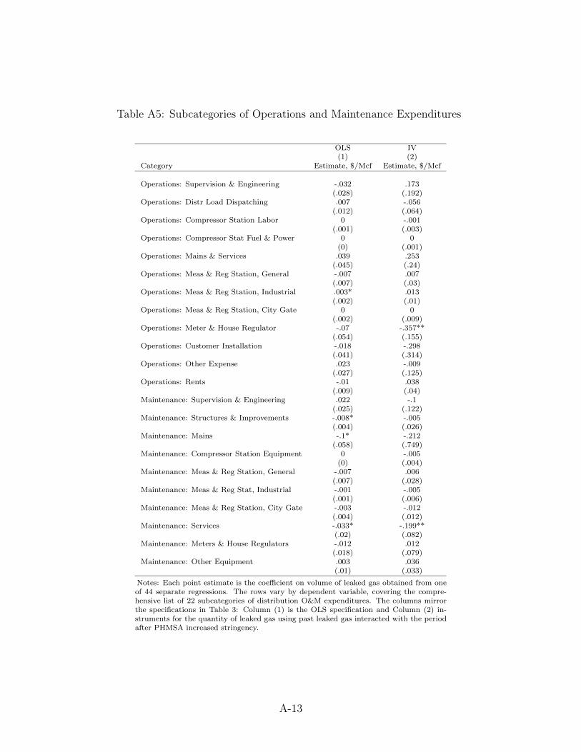
Table A5: Subcategories of Operations and Maintenance Expenditures

OLS IV(1) (2)

Category Estimate, $/Mcf Estimate, $/Mcf

Operations: Supervision & Engineering -.032 .173(.028) (.192)

Operations: Distr Load Dispatching .007 -.056(.012) (.064)

Operations: Compressor Station Labor 0 -.001(.001) (.003)

Operations: Compressor Stat Fuel & Power 0 0(0) (.001)

Operations: Mains & Services .039 .253(.045) (.24)

Operations: Meas & Reg Station, General -.007 .007(.007) (.03)

Operations: Meas & Reg Station, Industrial .003* .013(.002) (.01)

Operations: Meas & Reg Station, City Gate 0 0(.002) (.009)

Operations: Meter & House Regulator -.07 -.357**(.054) (.155)

Operations: Customer Installation -.018 -.298(.041) (.314)

Operations: Other Expense .023 -.009(.027) (.125)

Operations: Rents -.01 .038(.009) (.04)

Maintenance: Supervision & Engineering .022 -.1(.025) (.122)

Maintenance: Structures & Improvements -.008* -.005(.004) (.026)

Maintenance: Mains -.1* -.212(.058) (.749)

Maintenance: Compressor Station Equipment 0 -.005(0) (.004)

Maintenance: Meas & Reg Station, General -.007 .006(.007) (.028)

Maintenance: Meas & Reg Stat, Industrial -.001 -.005(.001) (.006)

Maintenance: Meas & Reg Station, City Gate -.003 -.012(.004) (.012)

Maintenance: Services -.033* -.199**(.02) (.082)

Maintenance: Meters & House Regulators -.012 .012(.018) (.079)

Maintenance: Other Equipment .003 .036(.01) (.033)

Notes: Each point estimate is the coefficient on volume of leaked gas obtained from oneof 44 separate regressions. The rows vary by dependent variable, covering the compre-hensive list of 22 subcategories of distribution O&M expenditures. The columns mirrorthe specifications in Table 3: Column (1) is the OLS specification and Column (2) in-struments for the quantity of leaked gas using past leaked gas interacted with the periodafter PHMSA increased stringency.

A-13

Table A6: Instrumenting for Pipeline Replacement: First Stage of Capital Cost Regression

(1)Low Quality Mains Replacement

Historic low-quality mains, miles 0.18***(0.03)

∆ volume sold, Bcf 0.24(0.38)

∆ mains, miles -0.05***(0.02)

∆ customers 0.00(0.00)

Region effects YesObservations 140Kleibergen-Paap F-stat. 40.02

Notes: Results show the first stage regression corresponding to Table 4. Depen-dent variable is the replacement of low quality mains from 2004 to 2013. Theinstrument is the miles of low quality mains in 2004. All variables are scaledby the utility’s average count of pipeline miles over the sample period. Robuststandard errors in parentheses. *** Statistically significant at the 1% level; **5% level; * 10% level.

A-14

Table A7: Cost of Pipeline Replacement: Robustness to Alternative Specifications

Total Capital Expenditures ($000)(1) (2) (3) (4) (5) (6) (7)

O&M+Capital All Capital Alt. Capital Capital Capital Capital CapitalLow-quality main replacement, miles 2,069*** 1,214** 1,232*** 1,229*** 1,479*** 1,571*** 1,868***

(792) (505) (407) (438) (562) (556) (313)Observations 140 140 129 141 79 136 140Kleibergen-Paap F-stat. 40.02 40.02 39.75 64.90 47.27 30.57 80.79

Notes: Column (1) includes O&M in addition to Capital. Column (2) includes all gas-related capital, not just distribution-specific gas-related capital. Column (3) uses an alternative reporting of capital: the change in accumulated capital rather than the sum of capitaladditions. Column (4) has no controls. Column (5) uses data from 1998 to 2013 instead of 2004 to 2013 and uses low quality pipes in1998 as the instrument. Column (6) weights by portion purchases made at the citygate (i.e., non-transmission and storage volumes).Column (7) does not scale. Robust standard errors in parentheses. *** Statistically significant at the 1% level; ** 5% level; * 10% level.

A-15

Table A8: Estimating an Emissions Factor: Volume Leaked on Miles Replaced

(1) (2)Volume Leaked Volume Leaked

Lagged low-quality mains, miles 400.46*** 573.18***(24.69) (67.22)

Lagged medium quality mains, miles 23.96 294.99**(15.65) (117.55)

Lagged volume sold 0.00*** 0.00***(0.00) (0.00)

Lagged pipeline mains, miles 15.18 -226.77*(31.85) (117.91)

Region-year effects Yes YesObservations 8,689 1,410R2 0.08 0.17

Notes: Dependent variable is the volume of leaked gas (Mcf). Column (1) in-cludes all data, not only the financial reporters. Column (2) only includes finan-cial reporters. Coefficient on “Lagged low-quality mains” in Column (2) servesas the emissions factor of gas leaked per mile of low-quality pipe, in Mcf/mile.Low-quality mains are those constructed of cast iron, ductile iron, or unprotectedbare steel and medium-quality mains are those constructed of copper, unprotectedcoated steel, or cathodically protected bare steel. The omitted category of mainsis high-quality mains: protected coated steel and plastic. All variables are scaledby the utility’s average count of pipeline miles over the sample period. Standarderrors are clustered by utility. *** Statistically significant at the 1% level; ** 5%level; * 10% level.

Table A9: Reported Leak Detection and Repair Costs

Type Estimate, $/Mcf

Reducing blowdown:Repairing valves during other repairs $1.20Composite wrap to prevent repairs $1.43Improved control system to reduce compressor start-ups $2.19Hot taps to reduce blowdown $3.93Capturing vented gas $5.55-6.67

Repairing leaks from compressors and pipes:Flexible plastic liners offsetCompressor stations $0.89Excess flow valves for new services $2.20Pneumatic devices, retrofit $2.93Pneumatic device, early replacement $7.11More frequent walking surveys $7.33

Reducing system pressure:Manually $1.95Automated depends

Notes: Source is EPA’s Natural Gas STAR program. All are 2009-2015.Accessed February 16 2016 from various “Fact Sheets” at the EPA’s “Rec-ommend Technologies and Practices – Natural Gas STAR Program” website,https://www3.epa.gov/gasstar/tools/recommended.html. Programs and equip-ment are assumed in this calculation to last one year, with the exception of ex-cess flow valves. Some documentation suggests 50-year lifetimes for excess flowvalves; here we have assumed a more conservative 25 year lifetime and a 3 per-cent discount rate.

A-16

Table A10: Reported Pipeline Replacement Costs

Type Source Estimate

Mains, Florida PUC1 170,000 - 190,000Cast iron, Allentown Newspaper2 650,000Cast iron, OH and KY Duke3 670,000Cast iron, Philadelphia NPR4 1 millionMains, Pennsylvania PUC5 200,000 - 1.8 millionBare steel, Ohio and New England Analysis Group6 300,000 - 1.2 millionMains, Philadelphia PUC5 1.5 millionCast iron, urban areas ICF for EDF7 1 - 3 millionCast iron AGA8 1.5 - 2.1 million

Notes: All are 2009-2015. Sources: 1Florida Public Service Commission, DocketNo 140166-GU. Order No PSC-14-0693-TRF-GU. Issued December 15, 2014.2www.lehighvalleylive.com. 2012. “Allentown, UGI differ over whether pace ofgas pipeline replacement is enough.” 3Duke Energy. 2012. “Lessons Learned froman Accelerated Main Replacement Program.” 4NPR. 2014. “Report: Philadelphiagas utility second worst for pipeline leaks.” 5Pennsylvania Public Utility Commis-sion. Staff Report. “Inquiry into Philadelphia Gas Works’ Pipeline ReplacementProgram.” April 2015. 6Aubuchon, Craig and Hibbard, Paul. “Summary of Quan-tifiable Benefits and Costs Related to Select Targeted Infrastructure ReplacementPrograms.” Analysis Group, Inc. January, 2013. 7ICF International. 2014. “Eco-nomic Analysis of Methane Emission Reduction Opportunities in the U.S. OnshoreOil and Natural Gas Industries.” Prepared for the Environmental Defense Fund.8American Gas Association website: https://www.aga.org/content/estimation-replacement-national-cast-iron-inventory-2012. Accessed April 19 2016.

A-17

Table A11: Damages from Accidents

OLS IV

(1) (2) (3)Damages ($) Damages ($) Damages ($)

Volume leaked, Mcf 0.08 0.02 0.19(0.07) (0.06) (0.26)

Low-quality mains, miles 607.94** -120.91 433.14(293.58) (301.68) (2,105.43)

Controls Yes Yes YesRegion-year effects Yes Yes YesUtility effects No Yes YesObservations 3,319 3,319 3,127Kleibergen-Paap F-stat. 14.01Implied leak abatement benefit, $/Mcf 0.08 0.02 0.19

(0.07) (0.06) (0.26)Implied pipeline replacement benefit, $/Mcf, F=229 2.65** -0.53 1.89

(1.28) (1.32) (9.19)Implied pipeline replacement benefit, $/Mcf, F=470 1.29** -0.26 0.92

(0.62) (0.64) (4.48)

Notes: These columns estimate the monetary damages from distribution pipeline accidents, i.e., the safety-relatedbenefits of accident prevention. Each column is a regression of monetary damages on leaks and on low-qualitymiles. Dependent variable is the aggregate of property damages, lost lives, using a Value of a Statistical Lifeof $9.1 million, and injuries, using a value of $1 million per injury. Column (3) instruments for both explana-tory variables using the interaction of historical count of low quality mains and an indicator for the period afterPHMSA regulations increased in stringency; and the interaction of historical volume leaked and an indicator forthe period after PHMSA regulations increased in stringency. The implied leak abatement benefits in $/Mcf forare simply equal to the coefficient on “Volume leaked, Mcf.” The implied pipeline benefits re-scale the coefficienton “Low-quality mains, miles” by an emissions factor, in Mcf/miles, of either 229 or 470. All three specificationscontrol for: region-year effects; total miles of pipeline mains; and total volume sold. All variables are scaled bythe utility’s average count of pipeline miles over the time period. Sample includes only utilities that ever re-ported an accident. Standard errors, in parentheses, are clustered by utility. *** Statistically significant at the1% level; ** 5% level; * 10% level.

A-18

Table A12: Robustness: Reduced-Form Estimates of What Explains Utility Expenditures

Alternative Specifications Specification Comparison

(1) (2) (3) (4)Total ($) Total ($) O&M ($) O&M ($)

Past volume leaked×I(Post-PHMSA) 1.33 0.35 0.30 0.21(1.51) (0.94) (0.39) (0.43)

Economic and Regulatory Variables:

City-gate price, $/Mcf -227 -37 -46(264) (168) (48)

Fraction of year in a rate case 1339** 1242** 307**(642) (618) (151)

Fraction of year in a rate-case test year 739 903* 179***(525) (457) (59)

I(Utility has pipeline rider) 2513** 1081 -35(1023) (831) (160)

Controls:Pipeline mains, miles 16038** -2629 836 1090

(7790) (1961) (757) (811)Service lines, count 11.85 23.32 3.76 9.32

(58.39) (23.40) (11.48) (13.33)Volume sold, Mcf -0.05 0.14 0.03 0.02

(0.18) (0.14) (0.03) (0.03)Low-quality mains, miles -2187

(4180)Low-quality service lines, count -28.35

(26.36)Region-year effects No Yes Yes YesYear effects Yes No No NoUtility effects Yes Yes Yes YesObservations 1,490 704 1,603 1,559R2 0.83 0.85 0.97 0.97

Notes: Regressions show the reduced-form regressions of expenditures on our instrument (theutility’s past leak volume interacted with the period that PHMSA increased regulatory strin-gency), along with other economic and regulatory variables. The dependent variable in the firsttwo columns is the sum total of capital and O&M expenditures in dollars. Columns show alter-native specifications to the total-expenditure regression found in Table 6: Column (1) includesyear effects instead of region-year effects. Column (2) uses a balanced sample of bundled-onlyutilities. The last two columns compare the estimates from the regressions exploring what drivesabatement with the reduced-form version of our main O&M estimation: Column (3) is the O&Mcounterpart of the previous three columns (this specification is also found in Table 6). Column(4) is the reduced form of our main estimation result (Table 3). All variables are scaled by theutility’s average count of miles of pipeline mains over the sample period, except price, fractions,and indicator variables. Standard errors are clustered by utility. *** Statistically significant atthe 1% level; ** 5% level; * 10% level.

A-19