Price Discrimination across Political Action Committees ...

Price Discrimination across Political Action

Committees: Evidence from the 2012 Presidential

Election

Sarah Moshary

⇤

July 7, 2015

Abstract

Political Action Committees have grown rapidly – expenditures neared $500 millionin the 2012 presidential election – emerging center-stage in the debate over money inAmerican politics. Their effect on elections depends on regulation and its interactionwith imperfect competition. Congress requires stations to treat candidates to the sameoffice equally, and to sell campaigns airtime at lowest unit rates (LURs) within sixtydays of a general election. This paper examines pricing to PACs, which are not protectedunder the law, and the impact of political advertising regulation. Using novel dataon prices paid for individual ad spots from the 2012 presidential election, I find thatstations price discriminate substantially across PACs for indistinguishable purchases.On average, PACs pay 40% markups above regulated rates. Republican PACs pay 14%higher prices on average relative to their Democrat counterparts, but there is substantialidiosyncratic variation in prices paid across ad spots. I develop and estimate a modelof political demand for ad spots, exploiting misalignments of state borders and mediamarkets to address potential price endogeneity. Findings indicate that pricing to PACsreflects buyer willingness-to-pay for viewer demographics. Taken together, these resultsindicate the current regulatory regime differentially subsidizes candidates depending onthe characteristics of their base.

⇤Department of Economics, MIT. Email: [email protected]. I would like to thank Glenn Ellison, NancyRose, and Paulo Somaini for invaluable help and advice throughout this project. I would also like tothank Nikhil Agarwal, Isaiah Andrews, Josh Angrist, Mark Bell, Vivek Bhattacharya, David Colino, Kath-leen Easterbrook, Sara Fisher Ellison, Ludovica Gazzè, Jerry Hausman, Mark Hou, Sally Hudson, GastonIllanes, Anna Mikusheva, Arianna Moshary, Casey O’Brien, Ben Olken, Manisha Padi, Brendan Price,Otis Reid, Miikka Rokkanen, Adam Sacarny, Richard Schmalensee, Amy Ellen Schwartz, Duncan Simester,Bradley Shapiro, Ashish Shenoy, Daan Struyven, Melanie Wasserman, Nils Wernerfelt, and participants inthe Industrial Organization seminar and field lunches at MIT.

1

Political Action Committee (PAC) spending in American elections skyrocketed to $1.3billion in 2012.1 This rise follows a series of Supreme Court decisions in 2010 eliminatinglimits on contributions to PACs.2 While the Federal Communications Commission (FCC)regulates television station sales of airtime to official campaigns, the law is silent on thetreatment of PACs. Station owners potentially wield considerable power to shape PACs’access to the airwaves. As an example, they might offer cheaper prices PACs that supporttheir favorite candidate. Alternatively, stations might charge PACs commensurately withtheir willingness-to-pay for airtime. Using novel data on television advertisement pricesfrom the 2012 presidential election, this paper investigates how TV stations set prices forPACs. I estimate PAC demand for airtime, and test whether and how much prices reflectwillingness-to-pay.

Pricing to PACs depends first on the extent of TV station market power. Stations typi-cally negotiate rates with commercial advertisers in an upfront market for ad spots, and theyare suspected of selling airtime at different rates to different advertisers. As an example,large purchasers may receive substantial discounts (Blumenthal & Goodenough 2006). Toensure candidates equal access to viewers, the FCC mandates all campaigns pay the sameprices for ad spots, set at lowest unit rates (LURs) (Karanicolas 2012).3 In contrast, news-paper headlines decry stations’ charging “super-gouge” rates to PACs. However, evidence onTV station pricing – to political or commercial advertisers – is thin.4

A first important finding is that on average, stations charge PACs 40% markups forairtime above the campaign price. Higher prices ought to temper the effect of PACs, sinceeach PAC dollar is worth less than its campaign counterpart. Second, in a comparison ofindistinguishable ads, Republican PACs pay higher prices than Democrat PACs (on the or-der of 14%), but there is substantial idiosyncratic variation in price differences across spots.While the literature (for example, Goettler 1999 or Bel & Domènech 2009) has documentedcorrelations between average prices and program characteristics, such as audience size, this

1I use PACs as an umbrella term for outside spending groups, including traditionalPACs, super PACs, and 501(c) organizations. Spending estimates come from OpenSecrets.org[https://www.opensecrets.org/outsidespending/fes_summ.php?cycle=2012].

2For a full description of contribution laws, see: the Federal Election Commission. “Federal ElectionCampaign Laws.” Washington, D.C.: 2008. Restrictions on donations to certain kinds of PACs remain.Crucially, there are no restrictions on donations to Super PACs, which accounted for 50% of spending in2012.

3Lowest unit rate rules come into effect within 45 days of a primary election and 60 days of a generalelection. The Federal Election Campaign Act of 1971.bl There is some ambiguity in implementation of thelaw. Law firms specialize in advertising law to help stations ensure they follow precedent.

4For example: Peters, Jeremy W., Nicholas Confessore and Sarah Cohen. 2012. “Obama is Even inTV Ad Race Despite PACs.” The New York Times. Oct 28. Bykowicz, Julie 2012. “TV Stations ChargeSuper-Gouge Rates for Super PACs.” Bloomberg News. Oct 6.

2

finding contributes to the limited empirical evidence that TV ad prices also differ substan-tially across buyers.5

Identifying the forces that drive ad pricing – and price differences across PACs – isessential to thinking about counterfactual regulatory regimes and evaluating current policy.One possibility is that station owners sell airtime more cheaply to the party they supportprivately. If owner bias were the primary driver of station pricing, then policy shieldingPACs could be crucial in guaranteeing voice to diverse political ideologies. I test whetherbias, measured by political donations, correlates with preferential pricing, but find littleevidence linking donations to pricing. Alternatively, prices may reflect viewer taste forPAC advertisements, as Gentzkow & Shapiro (2010) find for print newspapers. Differencesin negotiation costs could also drive pricing, as Goldberg (1996) finds for used-car dealertransactions with women and minorities. It may be that Republican PACs purchase airtimecloser to run-dates, and this timing element accounts for price differences. I examine a fifthpossibility: that stations price based on PAC taste for viewer demographics.

I develop a model of station price discrimination based on PAC willingness-to-pay fordifferent demographics, and test whether station behavior is consistent with this model. Thekey ingredients for this test are Democrat and Republican PAC preferences for viewership.These preferences depend on the strategy PACs pursue; for example, a get-out-the-vote strat-egy involves PACs targeting their base, whereas a persuasion strategy necessitates targetingswing voters.6 To estimate PAC preferences, I exploit the sensitivity of political demand tostate borders. Some ad spots bundle viewers in contested and uncontested states; politicaladvertising demand ought to be orthogonal to viewership in the latter. Since commercialadvertisers value these extra viewers, audiences in uncontested states constitute a residualsupply shock for political advertisers. Results provide evidence both of vote buying, whereparties target swing viewers, and turnout buying, where parties target their bases.

Since estimation imposes no model of supply-side behavior, I construct a test of whetherobserved prices are consistent with a model of station price discrimination based on PACwillingness-to-pay. My main finding is that model-generated utility estimates strongly cor-relate with observed prices. This relationship is robust, even controlling for costs and un-observed quality, suggesting stations do price discriminate and charge higher prices for adsPACs value most. Estimates employ lowest unit rates to measure cost, since these approxi-mate the opportunity cost of selling airtime to PACs.

5An older literature considered quantity discounts in television advertising, see Bagwell (2007) for adiscussion.

6 See Nichter (2008) for a complete categorization of strategies.

3

Taken together, my findings suggest lowest unit rate regulations benefit campaigns thatprize demographics unfavored by commercial buyers. For these campaigns, regulated ratesare likely to be far below their willingness-to-pay. Parties able to channel donations throughcampaigns also benefit disproportionately. If redistribution across parties and campaignsis desirable – for example, from candidates with a small number of wealthy supporters tocandidates with a large, but less affluent base – this may be interpreted as a regulatorysuccess story. Further, it suggests that under the current regime, market forces, rather thanmedia bias, drive inequalities in access to viewers for PACs; this distinction is potentiallyimportant in shaping future PAC regulations.

The paper proceeds as follows. Section 1 describes the data sources and construction ofkey variables for my analysis. Section 2 provides reduced-form evidence on price discrim-ination across PACs. Sections 3.1 and 3.2 develop a model of PAC demand for ad spots.Sections 3.3-3.5 lay out my estimation strategy, which exploits state borders to recover de-mand parameters. Results on PAC taste for viewer characteristics are presented in section3.6. Section 4 outlines a model of station price discrimination, and tests whether the modelis consistent with observed prices. Section 5 concludes.

1 Data

In this section, I detail the three main data sources used in this study: an online FCCdatabase on ad prices, Simmons survey data on viewership, and US Census data on marketdemographics. Then I describe statistics on viewership derived from the combined datasources.

1.1 Data Sources

The primary data for this paper is scraped from a newly mandated Federal Commu-nications Commission online database. As of August 2nd, 2012, stations in the 50-largestDesignated Market Areas (DMAs) are required to post detailed information about politicalad sales online. This requirement only holds for the four largest stations in each DMA: CBS,NBC, ABC, and FOX affiliates.7 The records include the station, client, media agency, showname, time, date, and purchase price for each transaction. Such detailed data is unique inthe advertising arena (see Stratmann (2009) for a description of standard data sources). The

7Federal Communications Commission. News Media Information. “FCC Modernizes Broadcast TelevisionPublic Inspection Files to Give the Public Online Access to Information Previously Available only at TVStations.” By Janice Wise. Washington, D.C: 2012.

4

extensive political science literature has employed fairly coarse data on prices in the past.As an example, researchers often impute ad exposure using campaign spending, potentiallyconfounding quantity with quality.8 CMAG’s (Campaign Media Analysis Group) data onad counts acquired via satellite technology is a popular alternative, but it contains no in-formation about prices. Other work has employed TV station logs, but until the adventof the FCC online archive, large-scale data collection was prohibitively expensive. To myknowledge, this is the first paper to exploit the newly-available ad buy data on the archive.

While this new data is incredibly detailed, it is not without flaws. Stations upload data ina variety of formats. Some stations post only order forms or contracts (which do not includethe specific date and time the ad is run, but only a date and time range), while others postactual invoices with as-run logs. The data quality varies by station; some stations haveposted low-quality scans of official documents. These forms are parsed less accurately byoptical character recognition software than are high-resolution documents. Therefore, thisdata is likely to be incomplete for stations that upload in this format (not that observed adsare misreported, but that the program misses some ads altogether).

Advertising data is paired with viewership data from Simmons, which is based on theirannual survey of 25,000 American households.9 Since ad spots are not a homogenous good– in the data they range in price from $10 to $650,000 – data on viewership is instrumentalin understanding pricing. Although ad spots are the unit of sale, advertiser demand is reallyfor viewers. The Simmons data allows me to deconstruct each ad into a collection of viewers.For each show, it contains the number of viewers by race, gender, and age.

The final data set contains 128,051 ad-level observations placed between August 1st andNovember 6th, 2012. This represents a subsample of the ads actually run over the courseof the entire election (approximately 15%)10 for four reasons: (1) OCR software imperfectlyparses photocopied invoices,; (2) ads purchased prior to August 1st are not required to appearon the website, and so are not included here; (3) the FCC only required the 200 stationsin the fifty largest DMAs to post on the website, excluding roughly 1,600 TV stations frommy sample;11 and (4) PACs explicitly focusing on non-presidential races are excluded fromthe analysis (approximately 16% of ads).12 The final sample includes ads placed by over 60political groups (42 pro-Republican and 20 pro-Democrat) at 37 TV stations in 19 DMAs.Table A1 shows the breakdown of ads by Political Action Committee.

8See Goldstein & Ridout (2004) for a detailed review of the literature.9Experian Marketing Services, Summer 2010 NHCS Adult Study 12-month. Simmons data is also used

by Martin & Yurukoglu (2014) to assess the relationship between media slant and viewer ideology.10Fowler & Ridout (2013) estimate 1,431,939 were run from January 1, 2012 to election day.11Fung, Brian. 2014. “A Win for Transparency in Campaign Finance.” The Washington Post. July 1.12I discard observations at stations without dual PAC and campaign advertising.

5

The sample appears to be fairly representative based on comparisons to Fowler and Rid-out’s (2013) description of Kantar Media/CMAG’s data. The CMAG sample includes alllocal broadcast, national cable, and national network ads for 2012, but contains no infor-mation about ad prices. As an example, the ratio of Romney to Obama campaign ads isthe same across the samples (approximately 2:5). Fowler and Ridout report that the aver-age price of an Obama campaign ad was strikingly lower than its Romney counterpart, apattern mirrored in my data (table 1). My sample includes a higher proportion of PACto candidate advertisements than the CMAG data. Fowler and Ridout designate ads as“presidential” based on content, while my criteria includes any ad purchased by PACs thatdonated to a presidential campaign, had a clear political affiliation, and did not explicitlysupport a candidate in another race. Categorization of PACs is based on records from theCenter for Responsive Politics.13

This new data on prices reveals important facts about the political ad market, and thescope for price discrimination. Figure 1 shows that prices (per viewer) increase in the run upto election day, consistent with stations’ extracting rent from political advertisers. Figure 2shows that advertising quantities also rise over time. Political groups are likely to value adsrun later in the cycle for myriad reasons: impressions decay quickly; many donations arrivelate in the election cycle;14 and the identities of swing voters may become clearer as theelection draws near. The average ad over the three-month period cost $1,260 and reachedsome 229,446 viewers.15

To get a sense of the importance of lowest unit rate regulation, I compute markupsfor PAC purchases above lowest unit rates during the 60 day period before the election.During this period, PACs (by law) pay weakly higher prices than campaigns.16 On average,Republican PACs pay 35% (standard error of 2.9%) markups and Democrat PACs pay46% (standard error of 4.6%) markups above lowest unit rates. These comparisons suggestLUR regulation provides a significant discount for campaigns. Candidates able to channelmoney through their official campaign therefore benefit most from regulation. Since current

13I conducted searches on OpenSecrets.org, maintained by the Center for Responsive Politics. In two cases,I obtained political affiliations based on newspaper articles linking groups to partisan advertising when theorganization was not categorized by OpenSecrets.org.

14In the 2012 presidential race, October was the most lucrative month for both parties, followed bySeptember, and then August (Ashkenas et al. (2012)).

15I winsorize prices (1%) to mitigate the effect of outliers in the rest of the paper.16Stations may try to circumvent regulation by redefining classes of time so that campaigns pay higher

prices than PACs for ads that tend to air at the same time. However, creating a campaign-specific class oftime is considered illegal. For some comparisons, campaigns therefore seem to be paying higher prices despitelowest unit rate rules (.2% or 22 out of 1,112 cases). I include these observations when calculating averagemarkups. (See Wobble Carlyle Sandridge & Rice, LLP. 2014. “Political Broadcast Manual.” Washington,D.C. By John F. Garziglia, Peter Gutmann, Jim Kahl and Gregg P. Skall.).

6

campaign finance laws restrict individual donations to campaigns, candidates with many,small donors can exploit regulation best.

1.2 Who Sees Political Ads?

Campaigns and PACs ultimately value winning elections. Ad spots are valuable becausethey reach viewers, viewers cast votes, and votes create winners. In this section, I estimatead exposures in the 2012 presidential race by combining survey data on viewership withmarket demographic data and data on ad purchases.

I infer ad viewership by marrying three data sources: FCC data on show names, times,stations, and networks; Simmons data on the viewing habits of different demographic groups;and 2010 census data on the population demographics by DMA. I match each purchased adspot from the FCC logs to viewership using show title or network and time (for exampleI assign average ABC 8am weekday viewership to all spots fitting that description withouta discernible show title). Matching without a specific name is useful since invoices oftendescribe purchases by these attributes rather than a “name.” Also, this matching strategyallows me to analyze new shows (premiering after 2010) although they do not appear directlyin the Simmons data.17

Let j denote the program and g denote a demographic group (e.g. white women under 65years of age). ⇡

gj

is the probability a member of group g sees ad j, approximated by countsfrom the Simmons data. Let J

cs

denote the set of ads broadcast in state s that supportcandidate c. Aggregating across this set produces total exposures for the demographic groupin state s supporting candidate c.

Agsc

=

X

j2Jcs

⇡gj

Variation in ad viewership across states comes from demographic differences and differencesin the composition of J

sc

(ad purchases), rather than preference heterogeneity within thesame group across states. Intuitively, in states with a higher proportion of individuals ingroup g, an ad that targets that group is more productive.

Estimated average exposures for each demographic group are displayed in table 2. Acrossall groups, viewers see approximately five times as many Republican PAC ads than theirDemocrat counterparts, which is consistent with Fowler and Ridout’s findings. Based on ad-airings by the 12 largest PACs in the 2012 race, they calculate that Democrat spots accountedfor 18% of political ads run. Interestingly, the skew in advertising is exacerbated at the

17This assumes demographics are stable across years for each time slot. If networks replace shows strate-gically, this matching algorithm will under-predict the value of ad spots that air during new shows.

7

exposure level; the difference in exposures across parties is higher than the ad counts wouldsuggest. Republican PACs not only buy more ads, but they also buy higher viewership ads.Although ad counts put the Democrats ahead, these exposure estimates suggest RepublicanPACs and the Romney campaign reached more viewers that the Democrat PACs and theObama campaign combined during the three months preceding the election.

Women see more political ads compared to men, and blacks see more spots compared toother racial groups. Both of these findings are in line with Ridout et al. (2012)’s tabulationsfor the 2008 election, and also with the broad TV watching habits of these demographicgroups. As an example, women are 20% more likely to watch a show than men (5.9%compared to 5%). Based on viewership habits, then, it seems reasonable that women alsosee approximately 20% more political ads than men.

These aggregate statistics, while hinting at PAC demographic targeting, confound adver-tiser preferences over demographics and TV viewing differences across these demographics.To understand how much variation in exposures is due to advertiser choice requires recon-structing the menu of potential ad buys, rather than simply looking at purchased spots.Data on rejected ad spots will allow me to determine how purchase decisions relate to view-ership composition. As an example, if rejected spots featured an even higher proportion ofwhite women than the set of purchased spots, then it seems unlikely that they are a coveteddemographic.

To construct the menu of potential spots, I partition each station-week into week-day/weekend spots, and then into 1-hour intervals (24 ⇥ 2 spots per station). However,Simmons only records viewership coarsely for early-morning shows, so I exclude programsairing between 12-5am, reducing the number of distinct products to 35 for each station,each week between August 1st and November 6th, 2012.18 Spot viewership depends on localdemographics and network programming. In total, there are 18,900 distinct products (36stations ⇥ 15 weeks ⇥ 35 day parts).

Ad spots are often also described by a priority level, and an indicator for which particulardays are permissible runtimes.19 Priority level characterizes how easily a station can preemptan ad, should they oversell slots on a show. While stations air preempted ads on anothershow with similar characteristics, industry wisdom is that so-called “make-goods” are worsequality (Phillips & Young (2012)). Low priority purchases constitute a gamble on the level ofresidual supply. Purchasers can also specify the day of the week for ad spots. As an example,an ad spot could be described as “Wednesday’s Today Show” or “Wednesday or Thursday’s

18During primetime, intervals narrow to 30 minutes. During early early morning, intervals are wider. Inthe simplest model, stations have a 168 products each week, one for each hour of each day.

19If the station records only invoices with “as-run” logs, then it is often not possible to determine thesecharacteristics of the purchase. I include a dummy in demand estimation as a flag for these missing values.

8

Today Show.” Rather than defining these combinations as separate commodities, I willcontrol for these features in demand estimation.20

2 Price Discrimination across PACs

Fear of inequitable media access across candidates is a key motivator for the regulationof political advertising (Karanicolas 2012). To shed light on whether these fears are wellfounded, I examine station behavior towards PACs, which is as yet unregulated. In par-ticular, I test whether Republican and Democrat PACs pay the same prices for the sameexact ad spots. To the contrary, I find that stations seem to price discriminate by politicalaffiliation.

2.1 Do Republican and Democrat PACs Pay the Same Prices?

In this section, I compare prices paid by Democrat and Republican PACs for indistin-guishable ad spots. It is unclear to what extent stations can tailor prices across differentpolitical buyers. Stations may lack the market power and information to price discriminateacross political advertisers. Indeed, if the market for airtime were perfectly competitive,lowest unit rate regulations would be irrelevant, since all buyers would pay the same pricefor airtime. Because the presidential race is a national one, network affiliates compete bothwithin and across DMAs for political dollars. High rates in one DMA would ostensibly in-duce substitution to other markets. More and more, stations also compete with other formsof media like Facebook and Twitter. Separate from competitive pressures, it is possible thatstations lack the information to price discriminate. The first task of this paper, therefore,is to examine the extent and type of station price discrimination across PACs. Apart fromproviding insight into a counterfactual world with less regulation, PAC advertising, whichnearly matched campaign expenditure in 2012, is itself an important piece of the competitiveelection puzzle.

I construct a price comparison for Democrats and Republicans using a restricted set ofad purchases. I consider cases where PACs supporting opposing candidates purchase airtimeon the same program (identified by name), for the same date, on the same station, andat the same hour.21 For this analysis, I treat the PACs supporting a particular candidateas a single entity, both for practical reasons (there are too few observations for one-on-onePAC comparisons) and also bearing in mind that like-minded PACs should value ad spotssimilarly, since they share an objective (elect their party’s nominee). A price-discriminatingstation should therefore charge these PACs similar prices. On the other hand, if stations

20For rejected shows, I assign characteristics in proportion to their presence in the purchased sample.21For this exercise, I consider only shows where the OCR software successfully scraped the full show name.

9

charge Democrat and Republican PACs similar prices for airtime, then it seems unlikelythat stations are discriminating (unless these groups share the same willingness-to-pay forviewers – in which case, stations would not be able to engage in taste-based discrimination).

Table 3 shows the results of this same-show comparison. There are 717 shows whereliberal and conservative PACs purchased exactly the same ad spots. In 212, they pay differentprices for those ads. The average price difference is $196.88, approximately 26% of the totalprice. While Republicans pay more on average ($68.41), Democrats are almost equally likelyto pay higher prices (among instances where Democrat and Republican PACs pay differentprices, Democrat PACs pay more almost 50% of the time). That neither Democrats norRepublicans pay more across the board suggests price discrimination is more complicatedthan simple party favoritism (for example, stations always charging Republican PACs more).

Regulation provides a nice placebo test for this exercise: since federal law prohibitsstations from charging the candidates different prices, the same comparison for the Obamaand Romney campaigns should yield zero price discrepancies. Of the 103 shows where bothcampaigns purchase, candidates only pay different prices for 20. Further investigation revealsthat half of these are errors in the data-gathering process (faults in the optical characterrecognition software). Reassuringly, the price differences between PACs are more than twiceas large for candidates, suggesting that the PAC price gap is more than a coding error.

I also examine within-party price differences for the 37 Republican PACs and 17 DemocratPACs in my data. For each ad purchased by multiple PACs with the same political affiliation,I calculate the coefficient of variation for prices (the standard deviation divided by the mean).Table 4 shows the mean coefficient of variation for the full sample in column (1). Pricedispersion is highest across parties. The coefficient of variation is 0.11 for the full sample ofdual Republican and Democrat purchases. The standard deviation, on average, is over 10%of the price. In comparison, the coefficient of variation is an order of magnitude smaller forwithin-party comparisons.

There is a potential selection problem in the column (1) comparison, since the coefficientof variation is measured conditional on purchase. As an example, constructing the coefficientof variation for Republican PACs for a particular ad spot requires at least two RepublicanPACs purchase the same ad spot. The set of ad spots used to construct the coefficientof variation therefore differs across comparison group. I recompute the estimates usingthe intersection of the three samples (Republican-Republican), (Democrat-Democrat) and(Republican-Democrat). For this sample, price dispersion can be calculated both withinand across groups. The estimates are presented in column (2). The qualitative results areunchanged. In fact, the coefficient of variation across parties grows. A test for whetherdispersion across parties is larger than dispersion within the Republican PAC group rejects

10

the null of equality at 5% (the t-statistic is 8.07).

2.2 Does Party Favoritism Explain Pricing?

Stations may charge Republican and Democrat PACs different prices for reasons separatefrom differences in PAC willingness-to-pay. As an example, station owners may offer cheaperrates to their favored party. To investigate this possibility, I examine whether station ownerand employees’ political donations are linked to ad prices, and in particular, whether stationswith a clear bias in donations have a similar bias in pricing. Data on donations comes fromthe Federal Elections Commission by way of the Sunlight Foundation.22 For each owner,I construct the percentage of donations given to Republicans compared to Democrats. Tomeasure bias in pricing, I construct a price dispersion index for each ad product sold toboth groups (again using the restricted sample), where p

D

and pR

are the Democratic andRepublican PAC prices, respectively.

=

pR

� pD

(pR

+ pD

)

I then average this measure across ads sold by the same media company (across stations andweek). A virtue of this index is that it measures price differences relative to the average costof the spot.23A value of 0 corresponds to no discrimination, while values of the close to 1(-1) indicate a strong pro-Democratic -Republican) bias in pricing.

Figure 3 shows that across owners, Democrats receive more favorable rates than Republi-cans. Across the five companies, ¯ ranges from .02 to .07, which corresponds to RepublicanPACs paying 4% to 15% more than their Democrat counterparts. Weigel Broadcasting,which is connected only to donations to Democrat affiliates, charges Republicans the largestmarkup. On the other hand, the Journal Broadcast Group, with gives 91% of donations toRepublican causes, still charges Republican PACs 7% more. Even within ownership com-pany, there is substantial variation in the Republican-Democrat price gap across ads. Thestandard errors for the estimated mean dispersion indices are large and clearly not statisti-cally significant. Nonetheless, the Republican - Democratic price gap that warrants furtherinvestigation using data on more media companies. Taken together, however, these resultssuggest observed price differences are not simply an artifact of station bias. This finding isconsistent with Gentzkow & Shapiro (2010), who find that newspaper bias explains only a

22The Sunlight Foundation maintains a database named “Influence Explorer,” which catalogues do-nations by individuals and political groups affiliated with each station’s parent company. Available:<data.influenceexplorer.com/contributions>.

23Others (for example, Daivs et al. (1996) and Chandra et al. (2013)) use this transformation in a similarspirit to prevent a few, large observations from skewing the measure of dispersion (or growth).

11

small part of media slant. Were rates set by the “most favorable” seller from a Republicanpoint of view, figure 3 indicates that Republican PACs would still benefit disproportionatelyfrom legislation prohibiting discrimination across political advertisers.

3 Political Demand for Ad Spots

Apart from media bias, price differences might reflect differences in willingness-to-payacross political ad buyers. Political parties may target different audiences depending ontheir strategy (Nichter (2008)).24 As an example, a vote-buying strategy involves persuadingindifferent voters to cast their ballot for your candidate. In contrast, a turnout buyingstrategy requires persuading folks who prefer your favored candidate to show up at thepolls. If both Democrats and Republicans attempt vote-buying, then they ought to valuesimilar demographics and the same ad spots. However, if at least one party focuses onturnout-buying, then Democrat and Republican preferences over demographics should bevery different. Pricing based on willingness-to-pay could also account for the observed pricedisparities within groups if PACs adopt different strategies.

To investigate whether stations price based on PAC willingness-to-pay for ad character-istics, I develop a model of demand for ad spots rooted in PACs’ allocating resources tomaximize the probability of winning. The first building block of the model specifies how ad-vertising affects voting. The second step embeds this vote production function into the PACad choice problem given a finite budget for advertising, and explicitly models the demandfor a particular ad spot. In section 3.3 and 3.4, I present an instrumental variable estimationstrategy for dealing with price endogeneity that exploits state borders. Section 3.5 discussesa selection correction for dealing with unobserved prices. I present results in 3.6, includingparameters governing party-specific taste for demographics.

3.1 Effect of Advertising on Voting

Let Vgsc

be the share of group g that votes for candidate c in state s. Vgsc

dependson ad exposures favoring candidate c, A

gsc

, and the efficacy of own advertising, �gc

. It alsodepends on opponent’s advertising, A

gsc

0 , and the efficacy of his advertising �gc

(for example,if his advertising convinces some viewers to switch allegiance or to stay home on electionday). The share of group g that votes for c also depends on the raw taste for the candidate�gsc

, and a random variable "sc

. "sc

induces aggregate uncertainty in voting outcomes, andis important in rationalizing advertising in states that are ex-post uncontested. Political

24Nichter (2008) details these strategies in the context of candidates or parties targeting benefits to par-ticular constituencies in return for voting behaviors. I adopt his terminology to describe ad targeting, whichis similar in spirit.

12

actors do not know which is the tipping-point state, the state whose electoral college votedecides the national election.25 Assume that these elements define a linear vote productionfunction.

Vgsc

= �gc

Agsc

� �gc

0Agsc

0+ �

gsc

+ "sc

(1)

Since electoral college votes are awarded in a winner-take-all fashion, political advertiserscare about producing votes only insomuch as it affects the probability their candidate winsa state’s majority.26 Their bottom line is the probability that S

sc

, the share of state s

that votes for candidate c, is larger than his rival’s share Ssc

0 . Ssc

is a function of ⇡gj

, theprobability a member of group g sees ad j, and f

gs

, the fraction of s’s population in groupg.

Ssc

=

X

g2G

fgs

Vgsc

= "sc

+

X

g2G

fgs

�gsc

+

X

g2G

fgs

�gc

X

j2Jcs

⇡gj

� �gc

0Agsc

0

!

Candidate c’s vote share aggregates baseline preferences and advertising effects across de-mographic groups, in proportion to their presence in state s. The probability that candidatec wins the state s therefore depends on the distribution of "

sc

and "sc

0 , own and rival’s adchoices, and state demographics:

P{Ssc

� Ssc

0}

= P("sc

� "sc

0 �X

g2G

fgs

(�gsc

0 � �gsc

) +

X

g2G

fgs

0

@(�

gc

0+ �

gc

0)

X

j2Jc0s

⇡gj

� (�gc

+ �gc

)

X

j2Jcs

⇡gj

1

A).

If I estimated (1) directly, then I could potentially estimate �gc

and �gc

separately (al-though individual-level voting data would be needed to estimate �

gsc

). �gc

is the effect ofcandidate c’s advertising on the proportion of the total population in state s and group g

that votes for him. �gc

is the effect of c’s advertising on his rival’s share. Winning the statedepends only on relative shares, so that candidates and PACs ultimately care about the sumof these two effects. Let �

gc

= �gc

+ �gc

. �gc

is the impact of c’s advertising on the differencein shares between the two candidates. This paper infers buyers’ demographic preferencesusing a revealed preference approach, so that only �

gc

, the net effect, is identified. Note that25In other words, the least favorable state their candidate must win to carry the national election. I borrow

Nate Silver’s estimates of tipping point probabilities from his New York Times blog. (Silver, Nate. 2012.“FiveThirtyEight Forecast.” <NewYorkTimes.com>. November 6.)

26In Nebraska and Maine, votes are split among districts. (FEC Office of Election Administration. “TheElectoral College.” By William C. Kimberling. 1992.)

13

while the vote production function is linear in advertising, the share of votes cast in c’s favor(the vote share) is not. The impact of advertising on candidate c’s vote share depends onthe stock of own and rival advertising.27

For tractability, let "sc

� "sc

0 distribute uniformly [�,], so that winning is describedby a linear probability model

P{Ssc

� Ssc

0} = +

X

g2G

fgs

(�gsc

� �gsc

0) +

X

g2G

fgs

✓�gc

X

j2Jcs

⇡gj

� �gc

0

X

j2Jc0s

⇡gj

◆.

The probability c wins state s is then an affine function of a weighted difference in adexposures (since �

gc

6= �gc

0) and the difference between the raw taste for candidates. Thisspecification of advertising technology exhibits constant returns to scale, which precludesinteractions between ad spots in vote production, but greatly simplifies demand estimation.Decreasing returns are embedded in the model since candidates can buy at most one adspot on each program on a station in a city. 28 This assumption is best-suited to ad choicein states where the margin between candidates is thin, so that the effect of advertising isplausibly locally linear. These are exactly the states with data for empirical study. Runningad j in support of c in state s changes the probability c takes the state by

�

jsc

=

X

g2G

fgs

⇡gj

�gc

.

To compare ads run in different states, I weight �jsc

to reflect states’ relative importance.Winning a state is only important inasmuch as it influences the likelihood of winning thenational election, and some states loom much larger in this calculation. A state’s importancedepends on its likelihood of being the tipping-point state, the least favorable state a candidatemust win to collect 270 electoral college votes. For the 2012 election, Nate Silver convenientlycalculated a tipping point index (⌧

s

) that gives the probability each state play this roll. Thisindex combines two forces that determine a state’s importance in a presidential election:first, the likelihood the state flips between red and blue, and second, the probability thenational outcome hinges on the the state outcome. The tipping-point index rationalizes, forexample, the dearth of campaigning in states like California or Texas with substantial heft

27Let Vsc

be the vote share of candidate c in state s.

Vsc

=

Pg

fgs

VgscP

g

fgs

(Vgsc

+ Vgsc

0)=

Pg

fgs

(Agsc

�gc

�Agsc

0 �gc

0)P

g

fgs

(�gc

Agsc

� �gc

0Agsc

0 + "sc

� "sc

0 + �gsc

� �gsc

0).

28Gordon & Hartmann (2013) utilize decreasing returns to scale of political advertising, but the returnsmay actually be convex – for cash-constrained campaigns, we may even see advertising on the convex partof the function.

14

in the electoral college. They have a low tipping-point index because the state outcome is aforgone conclusion.29 In sum, the effect of ad j in support of c in state s is v

jsc

:

vjsc

= ⌧s

�

jsc

=

X

g2G

fgs

⇡gj

�gc

. (2)

3.2 Ad Selection

The political advertiser employs (2) in choosing ads to maximize the probability hercandidate wins, subject to a budget constraint B. Let p

jstc

be the price of ad j run in states at week t in support of candidate c. J

sc

is the set of chosen ads. The optimization problemis described by:

max

{Jsc}Ss=1

P{c wins the election}

st:X

{j2Jsc}Ss=1

pjtsc

B

If advertisers can buy fractional ads, optimal purchasing follows a simple decision rule. If⌧s

�jsc/pjstc � ↵c

, then she should buy, where

↵c

= max

j /2{Jsc}Ss=1

(⌧s

�

jsc

pjstc

)

is the highest utility per dollar among ads not purchased.3031 In other words, buy adsin descending order of utility per dollar until the budget is exhausted. Purchased ads thenobey this decision rule. ↵

c

is naturally interpreted as the marginal utility of a political dollar.Although fractional purchases are permitted, this specification generates unit demand exceptfor the marginal ad at the cutoff.

The unknown parameters of this model are the effectiveness parameters, {�gc

}Gg=1, and

the shadow value of funds, ↵c

. To estimate these parameters, I incorporate two unobservablecomponents into ad value: ✏

jstc

, known only to buyers, and ⇠jstc

, known to buyers and sellers.The econometrician observes neither. ✏

jstc

introduces uncertainty, on the part of the station,29In states of the world where Texas or California changes hands, their electoral college votes are gratuitous

(extraneous to winning).30Without fractional purchases, set-optimization is challenging because it involves linear programming

with integer constraints.31Instrumental to developing a tractable demand model is the assumption that PACs take tipping-point

probabilities as given. As an example, a PAC assumes that even if it poured resources into California, itcould not change the probability that California is the decisive state in the national election.

15

as to exactly which ads political buyers value most, creating a downward sloping demandcurve. ⇠

jstc

accommodates the typical concern in demand estimation that stations andadvertisers have information about ad spots reflected in prices and quantities, but hiddenfrom the econometrician. An ad product is identified by j, the program name, s, the statewhere it airs, and t, the week it airs. The price of the product is buyer-specific, so italso has a subscript c. To recast the model using simpler notation, let x

jst

be the observablecharacteristics of an ad and (�

c

,↵c

) be the taste parameters of the party supporting candidatec. Then this model of purchasing behavior can be described by the latent utility of each adjstc:

u⇤jstc

= xjst

�c

� ↵c

pjstc

+ ⇠jstc

+ ✏jstc

.

Let yjstc

be an indicator for purchasing using the cutoff decision rule.

yjstc

= 1{u⇤jstc

� 0}. (3)

If ✏jstc

⇠ U [��,�], then (3) becomes a linear probability model

P{yjstc

= 1} =

1

2

+

xjst

�c

� ↵c

pjstc

+ ⇠jstc

2�

.

3.3 Instrument for Price

In this section, I propose an instrument for price to facilitate estimation of the PACdemand parameters from the preceding section. The goal is to estimate separate parametersfor Democrat and Republican PACs. Recovery of these preferences permits investigation ofhow observed prices relate to PAC willingness-to-pay.

The difficulty in estimating demand parameters is two-fold: first, prices are only observedfor purchased ads, and second, those prices are potentially correlated with the unobservable(E[⇠

jstc

|pjstc

] 6= 0). Endogeneity is a concern if stations price using information about adquality that is unknown to the econometrician.

Putting aside the first difficulty of transactions data, estimation requires an instrumentalvariable. To find a suitable instrument, I exploit a unique feature of presidential politicaladvertising: its sensitivity to state borders. DMAs often straddle state lines, so that viewersin different states are bundled together into a single ad spot. Ads with out-of-state viewersought to be more valuable (relative to the same ad run without these extra viewers) to run-of-the-mill TV advertisers, thus raising the opportunity cost of selling to a PAC. Viewershiplevels in uncontested states do not affect the value of an ad to a PAC, so the number of“uncontested” viewers, as a shifter of the residual supply curve, is an appropriate instrument

16

for political demand.The misalignment of media markets and political boundaries has been used to assess other

questions in political media, however not in an explicit instrumental variable approach. As anexample, Snyder Jr & Strömberg (2010) use the geography of newspaper markets to assesswhether media coverage disciplines politicians.32 Ansolabehere et al. (2001) investigatewhether congressional advertising on television declines in districts with more incidental(uncontested) viewers.33

The analogous ideal experiment is random assignment both of the distance of a DMAto a state border and the distribution of demographics across that border. Then ads nearborders with valuable neighbor demographics would have higher opportunity costs for reasonsunrelated to their political value. This instrument varies both within and across DMAs, sinceuncontested viewership depends on show demographics, state demographics and borders. Inmy sample, there are seven DMAs that broadcast to viewers in contested and uncontestedstates: Boston, Cincinnati, Denver, Jacksonville, Philadelphia, Pittsburgh and Washington,DC. Across these DMAs, ads reach a ratio of 1.2 uncontested viewers for each contestedviewer. Figure 5 shows the geography of DMAs in the sample which broadcast to bothcontested and uncontested viewers.

As an example, in the 2012 election, the Boston DMA received substantial advertisingbecause ads broadcast in Boston reach not only Massachusetts, but also New Hampshireviewers. The exclusion restriction is that Massachusetts viewership does not directly enterthe PAC demand specification. The relevance condition requires Massachusetts viewershipenter the demand of other advertisers, so that shows broadcast in Boston with higher Mas-sachusetts viewership have a higher opportunity cost.

The exclusion restriction is violated if PACs care about influencing other elections, eitherbecause they directly support candidates to other offices or if there are positive spilloversbetween presidential and congressional advertising. In that case, viewers in states wherethe presidential election is a foregone conclusion might be valuable if the senate seat is upfor grabs. I therefore include viewership in states with close senatorial races as an explicitdemand characteristic. The exogenous variation in price comes from variation in viewershipin states where neither the senatorial nor presidential race is contested.34

32They find that higher congruence between political and market boundaries leads to more local politicalstories, better informed constituents, and changes in House representatives’ behavior.

33They find that congresspeople in districts with more incidental viewers do not spend more on advertising,suggesting a strong, robust relationship between the price of airtime and purchasing behavior. I take thenext step, and exploit this relationship in an IV specification.

34This assumption might be violated if PACs purchase ads in an effort to fundraise in uncontested states.

17

3.4 Estimating Equations

The final demand specification is estimated separately for Democrat and RepublicanPACs. An ad product is a week-hour-station-weekend combination, where weekend is anindicator for Saturday or Sunday airtime. Demographic groups include the number of viewerswho are female, black, white, and over 65 years old. For each group, I include f

gs

⇡gj

, thefraction of the state in demographic group g watching program j. Ad prices and demographiccomposition are measured per contested viewer.35 k

jsct

includes controls: week dummies,and priority level36 fixed effects, and the proportion of viewers living in states with contestedsenate races.37 All demographic variables are multiplied by viewers’ average tipping-pointprobability ⌧

s

. The following system describes demand

pjstc

= �0c + �1c⌧s + �2czjs +GX

g=1

⌧s

fgs

⇡gj

�gc

+ k0jstc

�3c + ⌘jstc

(4)

yjstc

= �0c + �1c⌧s � ↵c

pjstc

+

GX

g=1

⌧s

fgs

⇡gj

�gc

+ k0jstc

�2c + ✏jstc

(5)

In practice, I use the two sample IV estimator from Angrist & Krueger (1995) with boot-strapped standard errors. I include predicted prices, which are fits from (4), in lieu of priceon the right-hand-side of (5). I estimate standard errors using the nonparametric bootstrap,since predicted prices are generated regressors. For robustness, I re-estimate the model withdaypart38 fixed effects, with an eye toward eliminating unobserved ad quality. Adding thesefixed effects means estimation exploits only within hour/week-segment variation.

3.5 Heckman Selection Correction

My estimation strategy so far ignores the selection problem inherent in transactionsdata: price is only observed for purchased ads. Censoring does not affect the estimation ofthe reduced form, but it means the first stage is estimated using only this sample. Showswith high draws of the instrument have higher prices, and correspondingly lower purchaseprobabilities. If I observe a high value of the instrument, I therefore ought to infer a lowdraw of the unobservable in the price equation. In the selected sample, this induces negative

35Normalizing by the number of viewers weighs ads equally. Otherwise, high markups on ads with lowviewership and low markups on ads with high viewership are observationally equivalent, despite there differenteconomic interpretations.

36For this part of the analysis, I restrict to four priority levels: p1, p2, p3+ and missing.37I use RealClearPolitics classification of “toss up” senate races in 2012 to measure whether a seat was con-

tested. States include: Indiana, Massachusetts, Montana, Nevada, North Dakota, Virginia, and Wisconsin.38e.g. 8 PM Weekend or 6 AM Weekday

18

bias in the estimation of the covariance between price and the cost shock.I can recast this inference challenge as the canonical problem of estimating labor supply:

attempting to estimate the impact of wages (prices) on labor force participation (purchasing),where wages (prices) are only observed for those who choose to work (purchase). In this spirit,this demand system can be rewritten as functions of an observed price p

jstc

and a latent pricep⇤jstc

that is only observed if yjstc

= 1.

p⇤jstc

= xjst

'1c + zjs

'2c + ⌘jstc

(6)

where zjs

is the instrument, and the observed price is truncated.

pjstc

=

8<

:p⇤jstc

if xjst

�c

� ↵c

p⇤jstc

+ ✏jstc

� 0

. if xjst

�c

� ↵c

p⇤jstc

+ ✏jstc

< 0

Heckman (1979) devised a selection correction assuming ✏, ⌘ distribute jointly normal withcovariance ⇢ . In this model

yjstc

= 1{xjst

�c

� ↵c

p⇤jstc

+ ✏jstc

� 0}

= 1{xjst

�c

� ↵c

(xjst

�1c + zjs

�2c + ⌘jstc

) + ✏jstc

� 0}

= 1{xjst

⇡1c + zjs

⇡2c + !jstc

� 0}

where ! = ✏� ↵⌘ ⇠ N(0,↵2�2⌘

+ �2✏

� 2↵⇢�✏

�⌘

), and �!

= 1 is the free scale normalization.This specification allows for price endogeneity through unobserved product quality.39 Esti-mation using Heckman’s two-step estimator permits recovery of the structural parameters:⇢, �

✏

, �⌘

, �gc

, �c

,↵c

. Note that without an exclusion restriction on z, we cannot separatelyidentify �

c

and ↵c

. It is important that z enter the selection equation only through its effecton prices, so that ↵

c

=

�⇡2�2

, and is just identified.The joint normality assumption is less than ideal. The bivariate normal distribution may

only poorly approximate the true distribution of unobserved PAC taste and cost shocks.A more serious concern is that the Heckman model specifies a structural pricing equationpotentially inconsistent with firm behavior. Price in (6) is a linear function of observedcharacteristics and an unobservable cost shock that distributes joint normal with the demand-

39Stata estimates �2⌘

and ⇢⌘!

, and lets �2!

= 1 as the scale normalization. We then need to rescale thestructural selection parameters using the standard deviation of the structural error term �

✏

. We can recover�✏

using the following two equations: �2!

= ↵2�2⌘

+ �2✏

� 2↵⇢✏⌘

�✏

�⌘

and ⇢⌘!

= cov(⌘,✏�↵⌘)�⌘�!

. Then we canestimate the variance of the structural selection equation as: �2

✏

= 2↵(�⌘

⇢⌘!

+ ↵�2⌘

)� ↵2�2⌘

. Note that thisallows for correlation between ⌘ and ✏, e.g. if there were unobserved (to the econometrician) product quality.

19

side taste shock. However, since selection is a serious concern with transactions data, theHeckman adjustment provides a sense of the magnitude of selection bias in this setting.

3.6 Evidence on Willingness-To-Pay for Democrat and RepublicanPACs

In this section, I discuss results about PAC preferences over demographics, which arepresented in table 5a (Republicans) and 5b (Democrats).

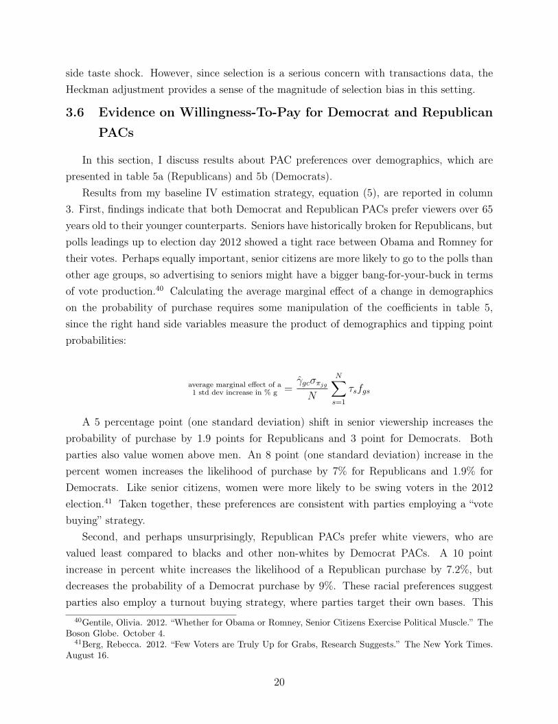
Results from my baseline IV estimation strategy, equation (5), are reported in column3. First, findings indicate that both Democrat and Republican PACs prefer viewers over 65years old to their younger counterparts. Seniors have historically broken for Republicans, butpolls leadings up to election day 2012 showed a tight race between Obama and Romney fortheir votes. Perhaps equally important, senior citizens are more likely to go to the polls thanother age groups, so advertising to seniors might have a bigger bang-for-your-buck in termsof vote production.40 Calculating the average marginal effect of a change in demographicson the probability of purchase requires some manipulation of the coefficients in table 5,since the right hand side variables measure the product of demographics and tipping pointprobabilities:

average marginal effect of a

1 std dev increase in % g

=

�gc

�⇡jg

N

NX

s=1

⌧s

fgs

A 5 percentage point (one standard deviation) shift in senior viewership increases theprobability of purchase by 1.9 points for Republicans and 3 point for Democrats. Bothparties also value women above men. An 8 point (one standard deviation) increase in thepercent women increases the likelihood of purchase by 7% for Republicans and 1.9% forDemocrats. Like senior citizens, women were more likely to be swing voters in the 2012election.41 Taken together, these preferences are consistent with parties employing a “votebuying” strategy.

Second, and perhaps unsurprisingly, Republican PACs prefer white viewers, who arevalued least compared to blacks and other non-whites by Democrat PACs. A 10 pointincrease in percent white increases the likelihood of a Republican purchase by 7.2%, butdecreases the probability of a Democrat purchase by 9%. These racial preferences suggestparties also employ a turnout buying strategy, where parties target their own bases. This

40Gentile, Olivia. 2012. “Whether for Obama or Romney, Senior Citizens Exercise Political Muscle.” TheBoson Globe. October 4.

41Berg, Rebecca. 2012. “Few Voters are Truly Up for Grabs, Research Suggests.” The New York Times.August 16.

20

is consistent with evidence from Ridout et al. (2012) on targeting in the 2010 midtermselections. If stations price based on willingness-to-pay, then the prices paid by Republicanand Democrat PACs should reflect the differences in their bases’ demographics.

Preferences for demographics are stable across IV specifications: column (4) reportsestimates including a full set of daypart dummies and column (5) reports coefficients witha Heckman selection correction. It is reassuring that these demand estimates are similar inmagnitude and sign to the baseline two sample least squares estimates. Since the qualitativeresults are not sensitive to the selection correction or the additional fixed effects, in theremaining analysis, I proceed with the IV baseline specification.

This model cannot tease apart different explanations for these preferences. PACs mayprefer women and seniors either because their underlying taste for candidates is more re-sponsive to advertising or because their turnout is more responsive to advertising – or both.The model combines both forces in mapping ad impressions to voting outcomes. However,these estimates reveal that preferences over demographics matter, both economically andstatistically.

Identification of PAC preferences across all specifications relies on uncontested viewershipmoving prices for reasons unrelated to political demand. Column (2) contains the first stageresults for the baseline model, which corresponds to estimating equation (4). I find a strongpositive correlation between uncontested viewers and prices, both for shows purchased byDemocrat and Republican PACs. The sign is consistent with a model where prices reflectcommercial demand. The F-statistics are 31.79 and 37.9 respectively, suggesting finite samplebias of these two stage least squares is small (Sock et al. (2002)).

The price coefficient in the second stage (column 3) is large and negative for both groups.In the baseline IV specification, Democrat demand elasticity (at the average ad programcharacteristics) is -1.28, and Republican demand elasticity is -0.969. In the absence of aninstrument, there is no variation in the purchase dummy conditional on price, so there anOLS regression of purchasing on price and characteristics is not possible. The closest OLSspecification merely shows the relationship between purchase probability and demographiccovariates (column 1). Unsurprisingly, including price as right-hand-side variable flips thesign on several of the viewer demographic coefficients, underscoring the importance of theIV strategy.

4 Price Discrimination Model

The big picture question are whether and to what extent willingness-to-pay matters forpricing, and whether the profit-maximizing station model explains pricing. Using demand

21

estimates (equation 5), I can measure willingness-to-pay for each ad spot and recover thesimple correlation for the sample of purchased ads. This simple test can provide sugges-tive evidence about how taste differences inform pricing decisions, but two factors confounda causal interpretation: marginal cost and unobservable quality. To illustrate how thesecombine if stations price based on buyer-specific taste for product characteristics (ad demo-graphics), I develop a structural model of station behavior in sections 4.1 and 4.2. Section4.3 creates machinery to test that model, which requires model-free estimates of markupsand model-generated optimal markups for comparison. Results are presented in section 4.4.

4.1 Monopoly Pricing with Lowest Unit Rate Regulations

The first step in the supply-side analysis is a simple model of stations as single-productmonopolists facing LUR regulations. This model informs the construction of bounds formarginal cost. Modeling marginal cost is important for testing whether observed pricesare consistent with taste-based price discrimination. If marginal cost is negatively correlatedwith willingness-to-pay, then failing to account for it in a regression of price on willingness-to-pay would camouflage price discrimination. On the other hand, if marginal cost is positivelycorrelated with willingness-to-pay, excluding costs could lead to false positives for pricediscrimination.

The marginal cost of an ad spot is opportunity cost – the highest price another advertiseris willing to pay for those 30 seconds. Intuitively, LUR rates, the lowest price for the spotsthat were purchased by campaigns, should approximate marginal costs well. This modelformalizes that intuition. The equilibrium conditions suggest LURs as an upper bound formarginal cost.

In determining how much to charge a PAC with demand PPAC

(QPAC

) for airtime, aTV station considers two other sources of demand for those same seconds: campaign ˜P (

˜Q)

and other, non-campaign demand P (Q) that might include other PACs. Non-campaigndemand is relevant because there are only T seconds of potential advertising time per show.Since airtime is not sold in a posted price market, I model the station as perfectly pricediscriminating against non-campaign advertisers.42 Campaign demand is separate becausestations are constrained to sell campaigns ads at the lowest price they command on themarket. The LUR regulation therefore forces stations to employ linear pricing schemes intheir dealings with campaigns. One consequence is that stations may not exhaust theircapacity, since selling additional units comes with a loss on inframarginal units sold to

42Stations sell most airtime in an upfront market each May. While they print “rate cards,” stationsnegotiate package buys with each buyer, chiefly through media agencies (Phillips & Young (2012)). Pricedisparities across PACs further motivates the perfect price discrimination assumption.

22

campaigns. In sum, the station faces the following constrained optimization problem

max

Q,Q

⇡ =

✓ˆQPAC

0

PPAC

(q)dq

◆+

✓ˆQ

0

P (q)dq

◆+

˜Q ˜P (

˜Q)

(LUR 1) st: P (Q) � ˜P (

˜Q) (LUR 1)(LUR 2) st: P

PAC

(QPAC

) � ˜P (

˜Q) (LUR 2)(Capacity Constraint) st: T � Q

PAC

+Q+

˜Q (Capacity Constaint)

Since the station can perfectly price discriminate against PACs and commercial adver-tisers, P ⇤

PAC

= P ⇤ in equilibrium. Therefore, either both LUR constraints bind or neitherbinds. Let ⇡¬PAC

be the profits from sales to campaigns and other advertisers:

⇡¬PAC

=

✓ˆQ

0

P (q)dq

◆+

˜Q ·min{P (Q), ˜P (

˜Q), PPAC

(QPAC

)}.

The opportunity cost is the change in ⇡¬PAC

from an increase in QPAC

� @⇡PAC

@QPAC

= �(P (Q)

@Q

@QPAC

+

˜P (

˜Q)

@ ˜Q

@QPAC

+

˜Q ˜P 0 @ ˜Q

@QPAC

). (7)

Condition (7) simplifies depending on which constraints bind. If and only if the stationsells positive quantities to a campaign, then the LUR binds. However, given data onQ

PAC

, PPAC

, ˜Q, ˜P , the econometrician does not know whether the capacity constraint binds.Given this information constraint, I bound marginal cost above by lowest unit rates. I showthis bound holds under the three sets of conditions that potentially describe equilibrium:

1. Both constraints bind. The CC implies @Q+Q/@QPAC = �1, so that (7) simplifies:

� @⇡PAC

@QPAC

= P (Q)� ˜Q ˜P 0 @ ˜Q

@QPAC

Determining the exact marginal cost requires assumptions on non-political ad demand(to estimate @Q

@QPAC). Without imposing such assumptions, I can bound the marginal

cost in the following fashion:

P (Q) >� @⇡PAC

@QPAC

> P (Q) +

˜Q ˜P 0(

˜Q)

Lowest unit rates overestimate marginal cost, since selling more units leads to infra-marginal losses on units sold to campaigns. Based on estimates of campaign demand

23

(tables 5a and b), ˜P 0(

˜Q) is small , so that the upper bound ought to be close to thetrue marginal cost.

2. Only the lowest unit rate rule binds. Selling additional units to the PAC forcesstations to lower LURs, which means inframarginal losses on units sold to campaigns.Marginal cost is less than the lowest unit rate since @Q+Q/@QPAC �1.

3. Only the capacity constraint binds. In this case, candidate demand is relativelylow compared to other advertisers so that ˜Q = 0. The equation for opportunity cost (7)becomes � @⇡PAC

@QPAC= P (Q), which is exactly the LUR. However, this rate is unobserved

since campaigns do not purchase any ads. It is possible that QPAC

= 0 if PAC demandfor that particular ad is also very low.

4. Neither constraint binds. This case never occurs so long as advertising has non-negative returns (and disregarding the disutility of viewers). If the LUR rule doesnot bind, that means campaigns are not purchasing airtime. At the very least, non-political advertisers and PACs should have positive value for airtime, and since stationscan perfectly price discriminate across units sold to these buyers, they should sell allof their airtime.

This model illustrates that lowest unit rates are a good proxy for marginal cost, albeit upperbounds. In the next section, I develop estimating equations based on the intuition from thismodel. In the final section, I incorporate LURs as marginal costs and explicitly test thestations’ first order conditions.

4.2 Station’s Optimal Pricing Condition

In this section, I adapt the continuous model to a discrete setting where the firm sells asingle indivisible unit of each product. This model is the simplest that permits examinationof price discrimination, the phenomenon of interest, but it may assign too much marketpower to stations. Since I have not imposed supply-side behavior in estimating demand, Ican test the monopoly assumption jointly with the demand estimates. If the model poorlyapproximates true station behavior – because stations lack market power, demand estimatesare incorrect, or pricing does not reflect PAC willingness-to-pay for demographics – thenobserved prices will be inconsistent with the monopolist’s FOC for pricing ad product (jst)to a PAC supporting c:

24

p⇤jstc

=

argmax

pjstc

(pjstc

� cjst

)(1� F✏

(�(xjst

�c

+ ⇠jstc

� ↵c

pjstc

)))

=) p⇤jstc

� cjst

=

1� F✏

(�(xjstc

�c

+ ⇠jstc

� ↵c

p⇤jstc

)))

↵c

f✏

(�(xjstc

�c

+ ⇠jstc

� ↵c

p⇤jstc

))

. (8)

This FOC ignores income effects by setting @↵c@pjstc

= 0. This assumption is standard in theIO literature for goods like ads that constitute but a small expenditure share of the budget(adding these effects restores complementarity between ad purchase decisions and greatlycomplicates both demand estimation and the pricing model). Essentially, I assume stationsignore cross-price elasticities. They assume that raising prices on a single ad has a negligibleeffect on demand for other ad buys. I also assume stations take tipping-point probabilitiesas given. This places the model somewhere on the spectrum between perfect competitionand monopoly. These assumptions are most suspect when considering counterfactuals wherethe price of airtime may rise across the board, but a substantial discrepancy between ob-served and predicted prices from a model without income effects would suggest taste-baseddiscrimination is unlikely to play an important role in this market.

This model incorporates three reasons for observed price differences between Democratand Republican PACs: different marginal utilities of money (↵

c

), different values for thesame demographics (�

gc

), and different values for other ad characteristics. It also pointsto another reason that Republican PACs pay higher prices on average: Republican PACsmay purchase higher cost ads. Since the set of ad-products purchased by both parties is aselected sample, understanding the cost-side is key for drawing conclusions about the winnersand losers under the current regulatory regime. To be clear, if differences in ad purchasedecisions account for the lion’s share of the difference in expenditures, then banning pricediscrimination across PACs ought to have but a small affect on the market. Conversely, ifpricing is driven primarily by willingness-to-pay, such regulation would have real bite.

Imposing ✏jstc

distributes uniformly simplifies the FOC (8), so that it is separable in thecost and preference-driven components of price:

p⇤jstc

=

�

2↵c

+

xjstc

�c

2↵c

+

cjst

2

+

⇠jstc

2↵c

(9)

4.3 Testing Station Optimization

To examine whether prices reflect PAC willingness-to-pay, I develop a series of tests basedon the TV station first order condition (8). As a first pass, I regress the observed price on

25

estimated utility per dollar separately for Democrats and Republican PACs. Willingness-to-Pay for each group is constructed using the demand parameters (ˆ�

c

and ↵c

) estimated via(5)

ujstc

=

xjst

ˆ�c

↵c

pjstc

= �0 + �1ujstc

+ ✏jstc

. (10)

This regression does not so much constitute a test of the particular monopoly model I proposeas a test of whether prices reflect preferences. If yes, the estimate of �1 ought to be large,positive and statistically significant.

If marginal costs are small and there is limited variation in unobserved quality, then(10) also constitutes a test of the structural model (9). However, marginal cost is usuallyassumed to rise with quality. In this market, if commercial advertisers and PACs value similarcharacteristics, then marginal cost ought to be positively correlated with PAC willingness-to-pay. Here, I employ LURs as a measure of marginal cost and re-estimate the first ordercondition including this term. To test the model, I test the null H0 : �1 =

12 , where �1 is

the coefficient on the “taste” component of pricing

pjstc

= �0 + �1xjst

ˆ�c

↵c

+ �2cjstc + ⌘jstc

. (11)

OLS estimation of (11) is still potentially biased due to selection on unobservables. Ifstations price according to the monopoly model, then the residual in (11) is a function ofunobserved ad quality: ⌘

jstc

=

⇠jstc

2↵c. Price is only observed conditional on purchase, so

that cov(⌘jstc

,xjst�c

↵c) 0 in this sample (though not the population). Intuitively, if a PAC

purchases an ad spot with poor observables, then that spot must have a high draw of theunobservable. This means OLS underestimates �

c

. The conditional expectation of pjstc

givenc purchases an ad with characteristics x

jst

is:

E[pjstc

|yjstc

= 1, x�,↵] =�

2↵c

+

xjst

ˆ�c

2↵c

+

cjst

2

+

E[⇠jstc

|yjstc

= 1]

2↵c

.

I can estimate the expectation of the omitted quality term if I specify a distribution for ⇠jstc

.Let ⇠

jstc

= �⇠

˜⇠ ⇠ N(0, �2⇠

). I model the CEF of ⇠jstc

conditional on observables xjst

, estimateddemand parameters ↵

c

, �c

, costs cjst

, and purchase at the optimal price. (Conditioning on

26

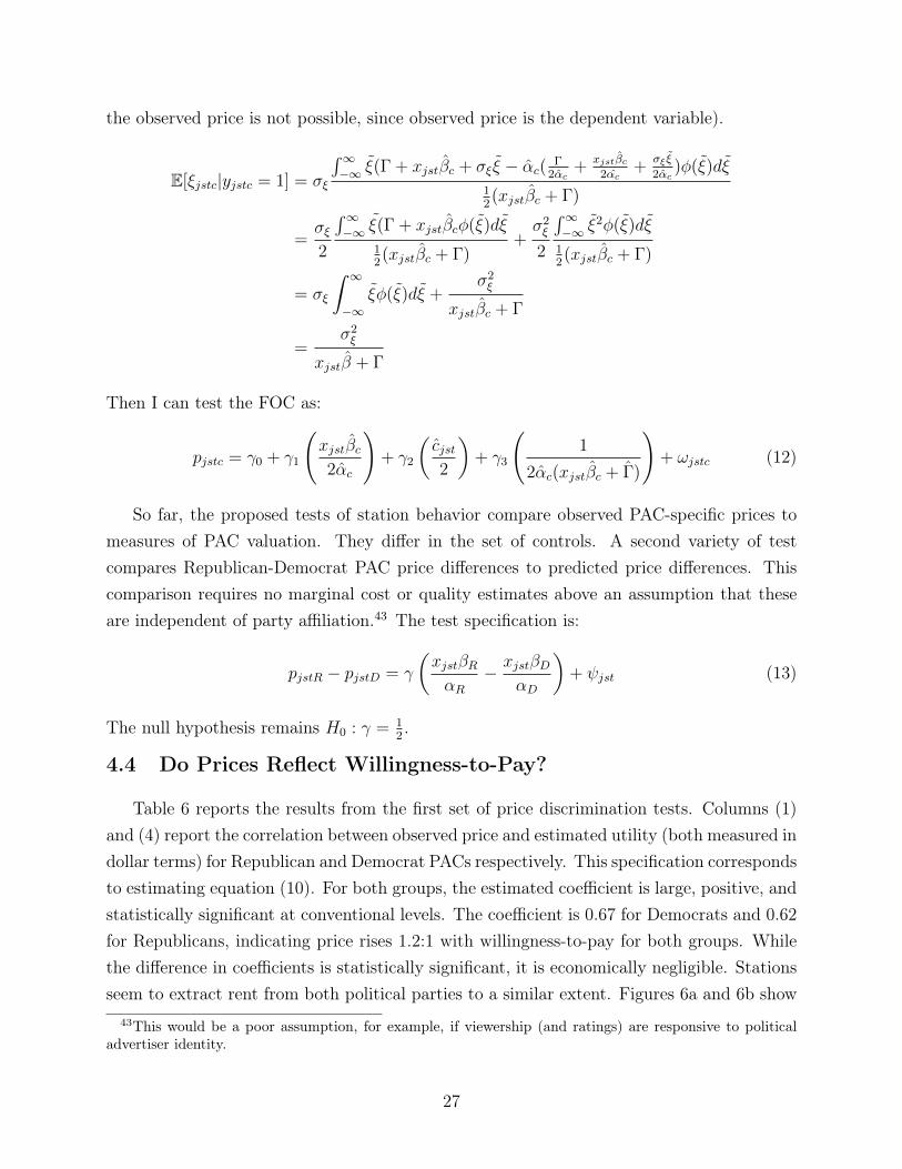
the observed price is not possible, since observed price is the dependent variable).

E[⇠jstc

|yjstc

= 1] = �⇠

´1�1

˜⇠(�+ xjst

ˆ�c

+ �⇠

˜⇠ � ↵c

(

�2↵c

+

xjst�c

2↵c+

�⇠ ⇠

2↵c)�(˜⇠)d˜⇠

12(xjst

ˆ�c

+ �)

=

�⇠

2

´1�1

˜⇠(�+ xjst

ˆ�c

�(˜⇠)d˜⇠

12(xjst

ˆ�c

+ �)

+

�2⇠

2

´1�1

˜⇠2�(˜⇠)d˜⇠

12(xjst

ˆ�c

+ �)

= �⇠

ˆ 1

�1

˜⇠�(˜⇠)d˜⇠ +�2⇠

xjst

ˆ�c

+ �

=

�2⇠

xjst

ˆ� + �

Then I can test the FOC as:

pjstc

= �0 + �1

xjst

ˆ�c

2↵c

!+ �2

✓cjst

2

◆+ �3

1

2↵c

(xjst

ˆ�c

+

ˆ

�)

!+ !

jstc

(12)

So far, the proposed tests of station behavior compare observed PAC-specific prices tomeasures of PAC valuation. They differ in the set of controls. A second variety of testcompares Republican-Democrat PAC price differences to predicted price differences. Thiscomparison requires no marginal cost or quality estimates above an assumption that theseare independent of party affiliation.43 The test specification is:

pjstR

� pjstD

= �

✓xjst

�R

↵R

� xjst

�D

↵D

◆+

jst

(13)

The null hypothesis remains H0 : � =

12 .

4.4 Do Prices Reflect Willingness-to-Pay?

Table 6 reports the results from the first set of price discrimination tests. Columns (1)and (4) report the correlation between observed price and estimated utility (both measured indollar terms) for Republican and Democrat PACs respectively. This specification correspondsto estimating equation (10). For both groups, the estimated coefficient is large, positive, andstatistically significant at conventional levels. The coefficient is 0.67 for Democrats and 0.62for Republicans, indicating price rises 1.2:1 with willingness-to-pay for both groups. Whilethe difference in coefficients is statistically significant, it is economically negligible. Stationsseem to extract rent from both political parties to a similar extent. Figures 6a and 6b show

43This would be a poor assumption, for example, if viewership (and ratings) are responsive to politicaladvertiser identity.

27

this relationship graphically. I group observations into 20 bins by percentile of estimatedutility, and plot each bin against its average price. The relationship appears strikingly linear.

Both the Democrat and Republican coefficients on willingness-to-pay are larger thanpredicted by the monopoly model. I can reject the null that the coefficient on is 0.5 forboth groups at the 5% level. A positive correlation between utility and cost could cause aninflation of the coefficient estimate, and explain rejection of the model.

Columns (2) and (5) control for marginal cost using lowest unit rates, which correspondsto equation (11). The coefficients on willingness-to-pay are closer to the model’s predictions.I cannot reject the null that the each coefficient is 0.5. The coefficients on cost, however, aresmaller than theory indicates, which dovetails with lowest unit rates as upper bounds formarginal cost. As a robustness check, I estimate test specification (12) which includes a proxyfor unobserved utility. Columns (3) and (6) present the results. Controlling for unobservedquality has almost no effect on the point estimates for the coefficient on willingness-to-pay,suggesting the variance in unobservable ad quality is small.

Table 7 reports results for the second set of tests, which compare observed price differencesto estimated utility differences. Price disparities are a prime motivator for concern aboutdiscrimination, so a stringent test of the model is whether it can replicate this facet of thedata. Column (1) reports the results of this test for the full set of ad-products where bothRepublicans and Democrats purchase. A $1 increase in Republican over Democrat utility perviewer corresponds to a $0.28 price hike for Republican versus Democrat PACs. Importantly,this test requires fewer assumptions on the cost side, since it lives only off of price differences.This small point estimate may be an artifact of the sample, since ad products are definedloosely as airtime at the same hour, station, and week. As an example, price differences mayreflect cost differences between high and low priority purchases, rather than utility differencesfor the same level of priority. Column (2) restricts the sample to indistinguishable goods,where priority level and show name must be an exact match. Reassuringly, the coefficientestimate increases to a $0.61 price increase per dollar of utility.

Selection remains a concern because I can only perform this test conditional on a pur-chase. The ideal regression would have differences in offered prices as the dependent variable,rather than differences in purchase prices. Selection could drive a correlation, in the pur-chased sample, between price and willingness-to-pay because buyers only purchase expensivespots when their willingness-to-pay is high. Under a pure selection story, however, stationssell both high and low willingness-to-pay slots to PACs at low prices; if stations success-fully price discriminate, they never sell high willingness-to-pay slots at low prices. Figure 8shows the distribution of transacted prices against willingness-to-pay; there are very few lowtransacted prices for the high WTP shows, consistent with a price discrimination story.

28

As a final test, I consider this relationship for the set of ad spots where stations activelyprice discriminate. In other words, I drop observations where Republicans and Democratspay the exact same price (approximately half of the observations). The results indicatea $0.79 increase in price difference per $1 increase in utility difference (results reported incolumn (4)). For this restricted sample, I cannot reject the null hypothesis that the monopolymodel is true (that a 1:1 relationship between utility and price differences hold).

Taken together, these results indicate a robust relationship between buyer-specific tastefor demographics and prices. Stations seem to be getting prices “right” by charging buyersmore for more-desired demographics. Although other forces undoubtedly factor into thepolitical ad market, including bundling and bargaining, my results suggest the monopolymodel approximates station behavior fairly well.

5 Conclusion

Since Lyndon B. Johnson’s infamous “Daisy” commercial aired in 1964, industry wisdomholds that paid TV advertising is necessary to a successful political campaign and, since1971, Congress requires television stations to sell airtime to all official campaigns at thesame price – in fact, at lowest unit rates (West 2010).44 Regulation advocates fear that,without restrictions, campaigns might face different prices, leading to large – and unfair –discrepancies in media presence. This paper examines station treatment of Political ActionCommittees, not subject to such restrictions, to shed light on whether, and to what extent,such fears are well-founded.

To be clear, PACs loom large on the political advertising scene – spending neared $500million in the 2012 presidential race – because campaign finance regulations require largedonations go through PACs.45 Importantly, stations have a free hand in their dealings withPACs, and their pricing decisions have direct consequences for inequalities in political speech.Further, the prices PACs pay can guide our expectations about prices official campaignswould pay absent regulation.

Novel data on ad-level prices reveals two stylized facts. First, PACs pay substantialmarkups above regulated rates. Since PACs face higher prices, a candidate should preferdonations come through his official campaign. When campaign finance regulation divertsfunds to PACs, the candidate gets a lower bang-for-his-buck. A candidate’s ad purchasingpower, therefore, depends on the distribution of donation dollars across his supporters. Sec-

44The Federal Election Campaign Act, 2 U.S.C. 431.45Ferrell, Stephanie, Matea Gold, Maloy Moorem, Anthony Pesce, and Daniel Schonhaut. 2012. “Out-

side Spending Shapes 2012 Election.” LA Times. Nov 20. <graphics.latimes.com/2012-election-outside-spending>.

29

ond, stations charge Democrat and Republican PACs different prices for indistinguishableads. Price differences have several potential causes: station owner bias, viewer preferencesover parties, differences in purchase timing, and PAC willingness-to-pay for ad characteris-tics, to name a few. I find little evidence that media bias, measured using data on politicaldonations, drives pricing. Rather, findings indicate that prices (and price differences) reflecteach party’s preferences for viewer demographics.

To recover PAC willingness-to-pay for different viewers, I develop a model of demand foradvertising spots and estimate preference parameters separately for Democrats and Repub-licans. To mitigate concerns about price endogeneity, I exploit the sensitivity of politicaldemand to state borders. Viewership in uncontested states constitutes a residual supplyshift for political advertisers. This permits identification of PAC demand curves under theassumption that PACs only value audiences in states that are potentially pivotal in the pres-idential election. Results suggest parties place a premium on the demographics of their base,which is consistent with a get-out-the-vote strategy.

Using these demand estimates, I develop and test a model of monopoly TV station be-havior. TV stations are widely thought to price discriminate in sales of airtime to commercialadvertisers, but this behavior has not been systematically studied in the literature. My find-ings confirm these suspicions; observed prices are consistent with a monopoly pricing model,indicating regulation actively prevents stations from price discriminating across candidates.Further, this result suggests lowest unit rate regulation differentially subsidizes candidatesin a second fashion. Regulation benefits candidates who prize viewer demographics that arerelatively undervalued by the commercial market. For these candidates, regulated rates arelikely to fall short of their true value for ad spots.

References

Angrist, Joshua D, & Krueger, Alan B. 1995. Split-Sample Instrumental Variables Estimatesof the Return to Schooling. Journal of Business & Economic Statistics, 13(2), 225–235.

Ansolabehere, Stephen, Gerber, Alan S, & Snyder, James M. 2001. Does TV AdvertisingExplain the Rise of Campaign Spending?

Ashkenas, Jeremy, Ericson, Matthew, Parlapiano, Alicia, & Willis, Derek. 2012. The 2012Money Race: Compare the Candidates.

Bagwell, Kyle. 2007. Handbook of Industrial Organization. 3(06).

Bel, Germà, & Domènech, Laia. 2009. What Influences Advertising Price in Television

30

Channels?: An Empirical Analysis on the Spanish Market. Journal of Media Economics,22(3), 164–183.

Blumenthal, Howard, & Goodenough, Oliver R. 2006. The Business of Television. BillboardBooks.

Chandra, Amitabh, Finkelstein, Amy, Sacarny, Adam, & Syverson, Chad. 2013. HealthcareExceptionalism? Productivity and Allocation in the U.S. Healthcare Sector.

Daivs, Steven, Haltiwanger, John C, & Schuh, Scott. 1996. Job Creation and Job Destruction.Cambridge: MIT Press.

Fowler, Erika Franklin, & Ridout, Travis N. 2013. Negative, Angry, and Ubiquitous: PoliticalAdvertising in 2012. The Forum, 10(4), 51–61.

Gentzkow, Matthew, & Shapiro, Jesse M. 2010. What Drives Media Slant? Evidence FromU.S. Daily Newspapers. Econometrica, 78(1), 35–71.

Goettler, Ronald. 1999. Advertising Rates, Audience Composition, and Competition in theNetwork Television Industry.

Goldberg, Pinelopi K. 1996. Dealer Price Discrimination in New Car Purchases: Evidencefrom the Consumer Expenditure Survey. Journal of Political Economy, 104(3), 622–654.

Goldstein, Kenneth, & Ridout, Travis N. 2004. Measuring the Effects of Televised PoliticalAdvertising in the United States. Annual Review of Political Science, 7(1), 205–226.

Gordon, Brett R., & Hartmann, Wesley R. 2013. Advertising Effects in Presidential Elections.Marketing Science, 32(1), 19–35.

Heckman, James J. 1979. Sample Selection Bias as a Specification Error. Econometrica,47(1), 153–161.

Karanicolas, Michael. 2012. Regulation of Paid Political Advertising: A Survey. Tech. rept.March. Centre for Law and Democracy.

Martin, Gregory J, & Yurukoglu, Ali. 2014. Bias in Cable News: Real Effects and Polariza-tion.

Nichter, Simeon. 2008. Vote Buying or Turnout Buying? Machine Politics and the SecretBallot. American Political Science Review, 102(01), 19–31.

31

Phillips, Robert, & Young, Graham. 2012. Television Advertisement Pricing in the UnitedStates. Pages 181–190 of: Ozer, Ozalp, & Robert, Phillips (eds), The Oxford Handbookof Pricing Management. Oxford: Oxford University Press.

Ridout, Travis N., Franz, Michael, Goldstein, Kenneth, & Feltus, William J. 2012. Sep-aration by Television Program: Understanding the Targeting of Political Advertising inPresidential Elections. Political Communication, 29(1), 1–23.

Snyder Jr, James M, & Strömberg, David. 2010. Press Coverage and Political AccountabilityDavid Stro. Journal of Political Economy, 118(2), 355–408.

Sock, James H., Wright, Jonathan H., & Yogo, Motohiro. 2002. A Survey of Weak Instru-ments and Weak Identification in Generalized Method of Moments. Journal of Business& Economic Statistics, 20, 518–529.

Stratmann, Thomas. 2009. How Prices Matter in Politics: the Returns to Campaign Adver-tising. Public Choice, 140(3/4), 357–3777.

West, Darrell M. 2010. Air Wars: Television Advertising in Election Campaigns 1952-2008.Fifth edn. Washignton, DC: CQ Press.

32

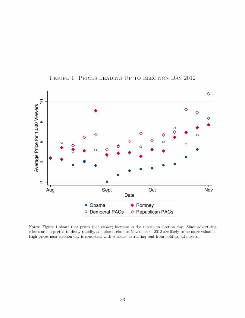
Figure 1: Prices Leading Up to Election Day 2012

24

68

10Av

erag

e Pr

ice

for 1

,000

Vie

wer

s

Aug Sept Oct NovDate

Obama RomneyDemocrat PACs Republican PACs

Notes: Figure 1 shows that prices (per viewer) increase in the run-up to election day. Since advertisingeffects are suspected to decay rapidly, ads placed close to November 6, 2012 are likely to be more valuable.High prices near election day is consistent with stations’ extracting rent from political ad buyers.

33

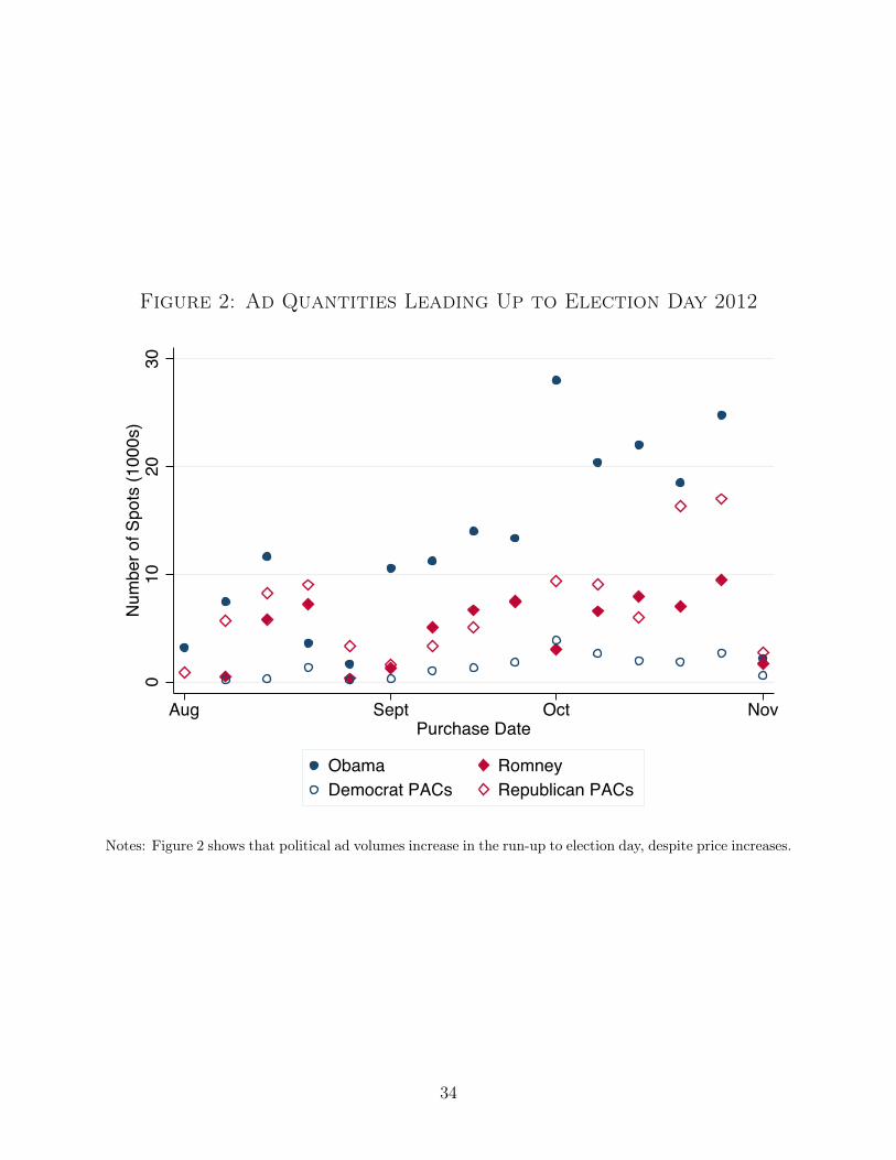
Figure 2: Ad Quantities Leading Up to Election Day 2012

010

2030

Num

ber o

f Spo

ts (1

000s

)

Aug Sept Oct NovPurchase Date

Obama RomneyDemocrat PACs Republican PACs

Notes: Figure 2 shows that political ad volumes increase in the run-up to election day, despite price increases.

34

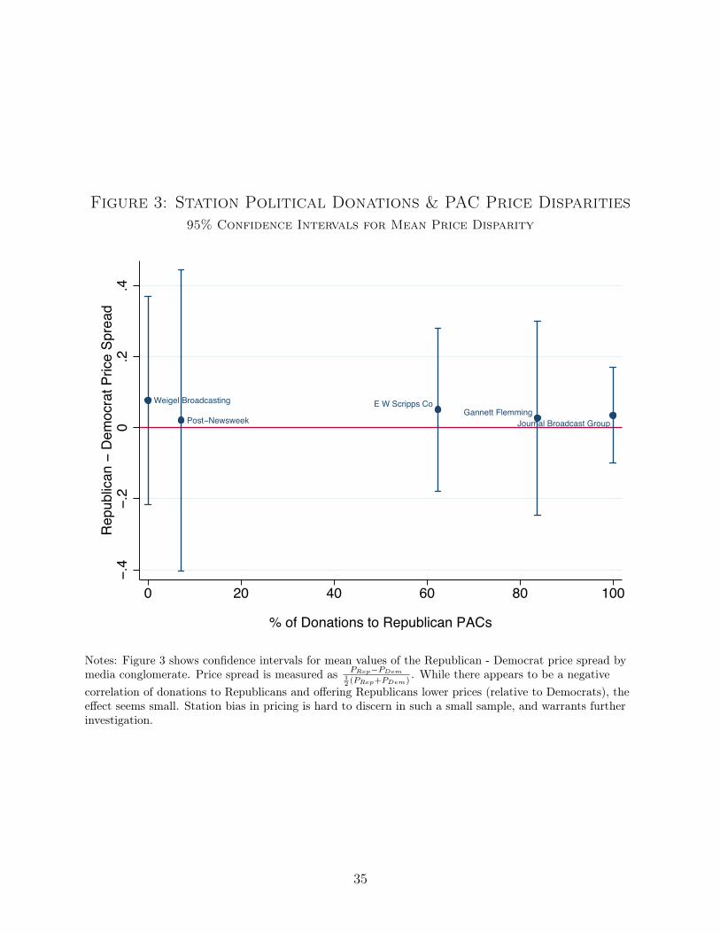
Figure 3: Station Political Donations & PAC Price Disparities

95% Confidence Intervals for Mean Price Disparity

E W Scripps CoGannett Flemming

Journal Broadcast GroupPost−Newsweek

Weigel Broadcasting

−.4

−.2

0.2

.4R

epub

lican

− D

emoc

rat P

rice

Spre

ad

0 20 40 60 80 100

% of Donations to Republican PACs

Notes: Figure 3 shows confidence intervals for mean values of the Republican - Democrat price spread bymedia conglomerate. Price spread is measured as PRep�PDem

12 (PRep+PDem)

. While there appears to be a negativecorrelation of donations to Republicans and offering Republicans lower prices (relative to Democrats), theeffect seems small. Station bias in pricing is hard to discern in such a small sample, and warrants furtherinvestigation.

35

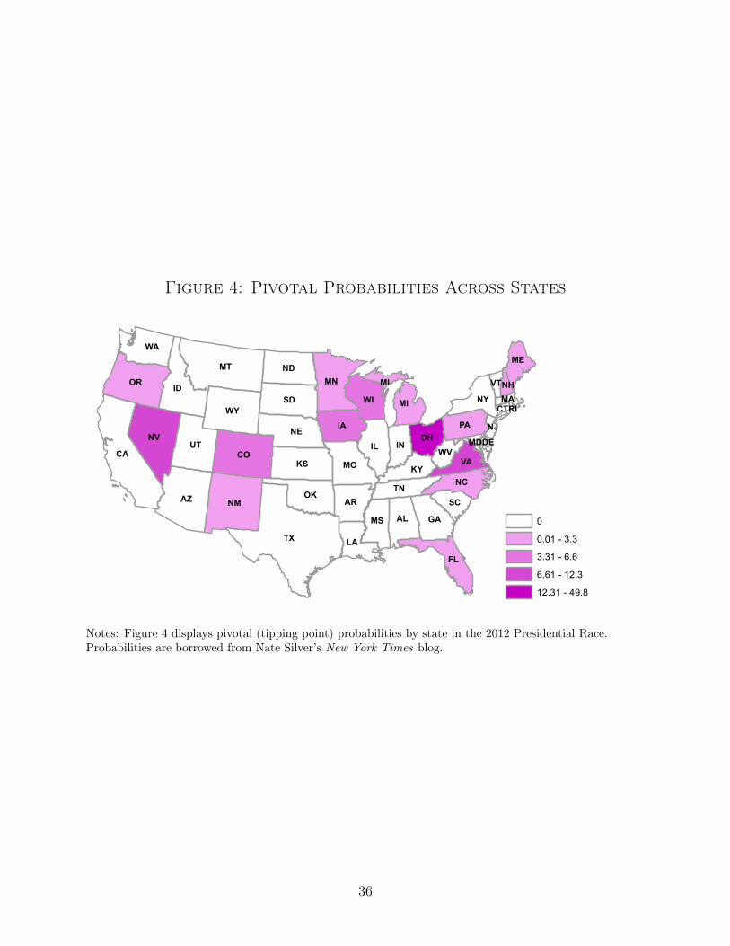
Figure 4: Pivotal Probabilities Across States

TX

CA

MT

AZ

ID

NV

NM

CO

OR

UT IL

WY

KS

IANE

SD

MNND

OK

WI

FL

MO

WA

GAAL

MI

AR

IN

PA

LA

NY

NC

MS

TN

VAKY

OH

SC

ME

WV

MI VTNH

MD

NJ

MACT

DE

RI

pivotal0

0.01 - 3.3

3.31 - 6.6

6.61 - 12.3

12.31 - 49.8

Notes: Figure 4 displays pivotal (tipping point) probabilities by state in the 2012 Presidential Race.Probabilities are borrowed from Nate Silver’s New York Times blog.

36

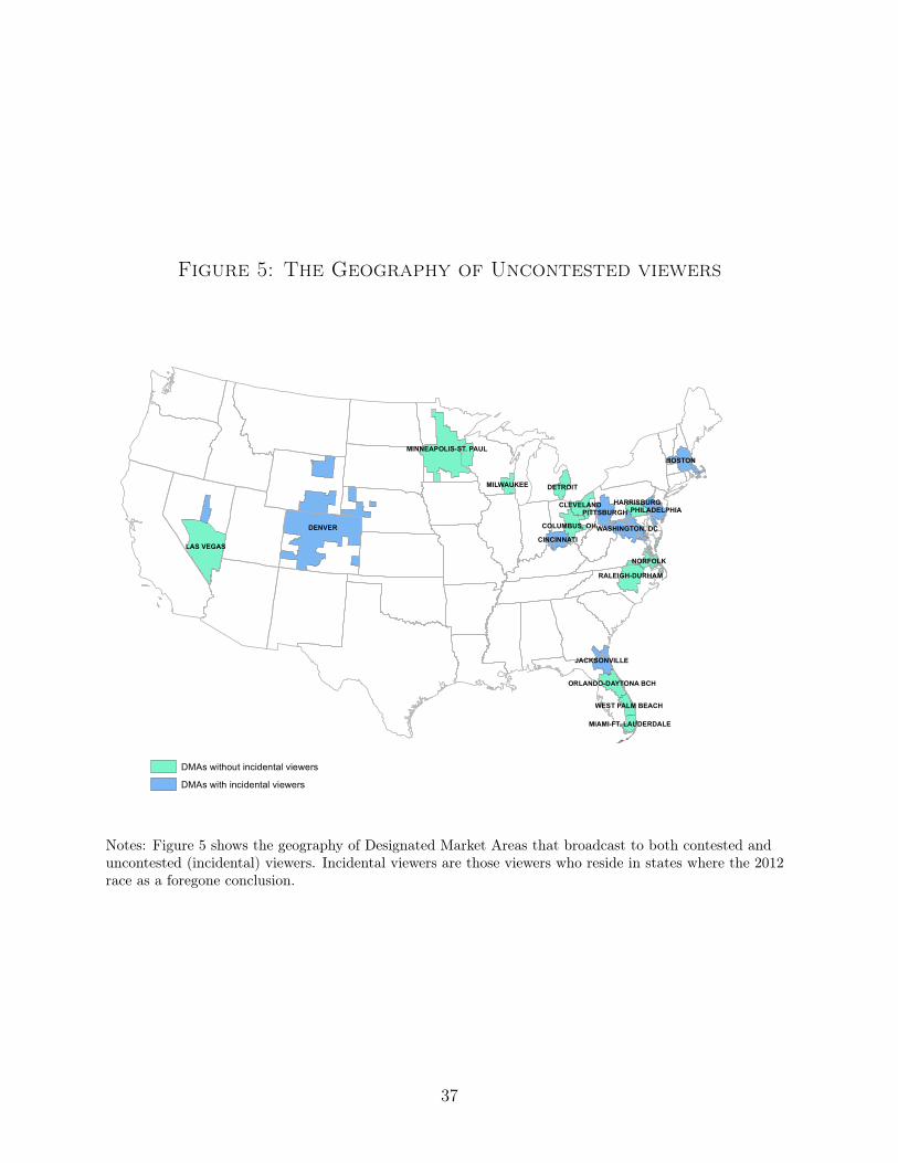
Figure 5: The Geography of Uncontested viewers

DENVER

LAS VEGAS

MINNEAPOLIS-ST. PAULBOSTON

PITTSBURGH

WASHINGTON, DC

DETROIT

CINCINNATI

RALEIGH-DURHAM

CLEVELAND

COLUMBUS, OH

PHILADELPHIA

JACKSONVILLE

NORFOLK

MILWAUKEE

HARRISBURG

ORLANDO-DAYTONA BCH

WEST PALM BEACH

MIAMI-FT. LAUDERDALE

DMAs without incidental viewers

DMAs with incidental viewers

Notes: Figure 5 shows the geography of Designated Market Areas that broadcast to both contested anduncontested (incidental) viewers. Incidental viewers are those viewers who reside in states where the 2012race as a foregone conclusion.

37

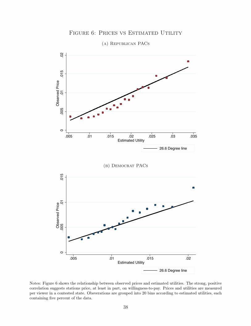
Figure 6: Prices vs Estimated Utility

(a) Republican PACs

0.0

05.0

1.0

15.0

2O

bser

ved

Price

.005 .01 .015 .02 .025 .03 .035Estimated Utility

26.6 Degree line

(b) Democrat PACs

0.0

05.0

1.0

15O

bser

ved

Pric

e

.005 .01 .015 .02Estimated Utility

26.6 Degree line

Notes: Figure 6 shows the relationship between observed prices and estimated utilities. The strong, positivecorrelation suggests stations price, at least in part, on willingness-to-pay. Prices and utilities are measuredper viewer in a contested state. Obsverations are grouped into 20 bins according to estimated utilities, eachcontaining five percent of the data.

38

Figure 7: Price Differences vs Estimated Utility Differences

(a) Full Sample

−.01

−.00

50

.005

.01

.015

Rep

ublic

an −

Dem

ocra

t Pric

e Pa

id ($

)

.001 .002 .003 .004 .005Republican − Democrat Utility ($)

45 Degree Line

(b) Interdecile Range

−.00

10

.001

.002

.003

Rep

ublic

an −

Dem

ocra

t Pric

e Pa

id ($

)

.001 .002 .003 .004 .005Republican − Democrat Utility ($)

45 Degree Line

Notes: Figures 7 (a) and (b) show the relationship between observed price differences and estimated utilitydifferences. Subfigure (a) shows the full sample, while (b) restricts to the interdecile range for legibility. Thestrong, positive correlation suggests differences in willingess-to-pay between Republicans and Democrats helpexplain the differences in observed prices. The comparison is conducted only for spots where Republican andDemocrat PAC purchases are indistinguishable. Prices and utilities are measured per viewer in a contestedstate. Obsverations are binned into groups of five percentiles.

39

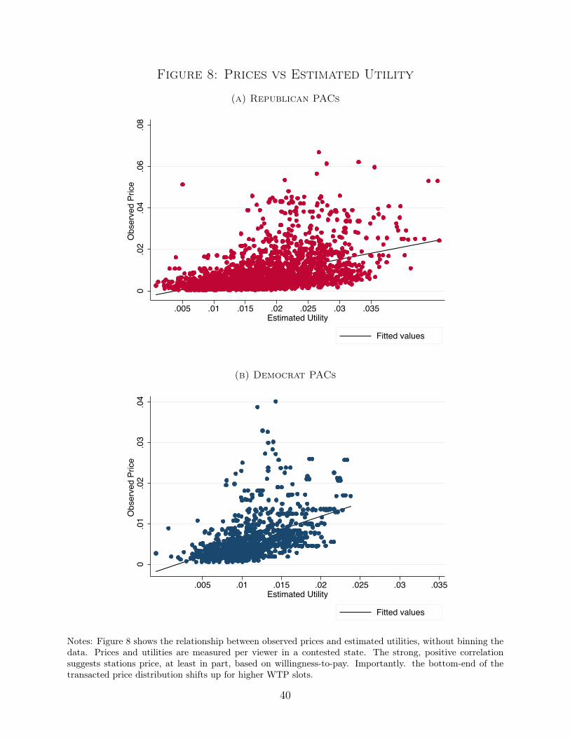
Figure 8: Prices vs Estimated Utility

(a) Republican PACs

0.0

2.0

4.0

6.0

8O

bser

ved

Pric

e


Fitted values

(b) Democrat PACs

0.0

1.0

2.0

3.0

4O

bser

ved

Pric

e


Fitted values

Notes: Figure 8 shows the relationship between observed prices and estimated utilities, without binning thedata. Prices and utilities are measured per viewer in a contested state. The strong, positive correlationsuggests stations price, at least in part, based on willingness-to-pay. Importantly. the bottom-end of thetransacted price distribution shifts up for higher WTP slots.

40

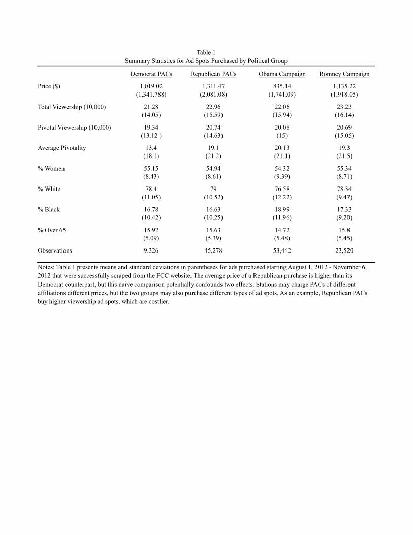
Democrat PACs Republican PACs Obama Campaign Romney Campaign

Price ($) 1,019.02 1,311.47 835.14 1,135.22(1,341.788) (2,081.08) (1,741.09) (1,918.05)

Total Viewership (10,000) 21.28 22.96 22.06 23.23(14.05) (15.59) (15.94) (16.14)

Pivotal Viewership (10,000) 19.34 20.74 20.08 20.69(13.12 ) (14.63) (15) (15.05)

Average Pivotality 13.4 19.1 20.13 19.3(18.1) (21.2) (21.1) (21.5)

% Women 55.15 54.94 54.32 55.34(8.43) (8.61) (9.39) (8.71)

% White 78.4 79 76.58 78.34(11.05) (10.52) (12.22) (9.47)

% Black 16.78 16.63 18.99 17.33(10.42) (10.25) (11.96) (9.20)

% Over 65 15.92 15.63 14.72 15.8(5.09) (5.39) (5.48) (5.45)

Observations 9,326 45,278 53,442 23,520

Summary Statistics for Ad Spots Purchased by Political GroupTable 1

Notes: Table 1 presents means and standard deviations in parentheses for ads purchased starting August 1, 2012 - November 6, 2012 that were successfully scraped from the FCC website. The average price of a Republican purchase is higher than its Democrat counterpart, but this naive comparison potentially confounds two effects. Stations may charge PACs of different affiliations different prices, but the two groups may also purchase different types of ad spots. As an example, Republican PACs buy higher viewership ad spots, which are costlier.

Men Women Men Women Men Women Men Women

White 11.73 13.62 8.55 10.26 59.32 68.32 42.89 51.21

Black 11.80 14.18 9.63 11.95 67.05 82.23 54.43 68.51

Other 8.30 9.60 6.17 7.40 39.54 44.84 28.40 33.73

Men Women Men Women Men Women Men Women

White 68.58 79.43 46.65 56.59 30.97 36.20 22.08 26.71

Black 84.75 102.41 63.61 80.21 36.33 45.02 29.29 37.31

Other 30.91 51.63 68.58 36.98 14.74 23.46 30.97 17.81

Notes: Table 2 calculates expected ad exposures for each of twelve demographic groups based on the purchases in my data. Exposures are calculated based on the programs where ads air and the proclivity of members of each group to watch those programs. The difference in exposure between the Obama and Romney campaign highlights the importance of outside spending in the 2012 election.

Romney CampaignObama Campaign

Ages 18-64 Ages 65+ Ages 18-64 Ages 65+

Table 2Estimated Ad Exposures in Tipping Point States by Demographic Group and Political Party

Republican PACsDemocrat PACs

Ages 18-64 Ages 65+Ages 18-64 Ages 65+

PACs Candidates(Republicans - Democrats) (Romney - Obama)

% Zero Price Difference 41.28 80.34% Higher Republican Price 30.26 8.28% Higher Democrat Price 28.45 11.38

Measure of Price Dispersion:\

Absolute Value of Price Difference 196.88 96.21(12.63) (12.98)

Absolute Value of % Price Difference 26 14(3.00) (2.00)

Raw Price Difference 68.41 -33.45(14.39) (14.02)

% Raw Price Difference 14 4(3.00) (3.00)

# Observations 717 290

Table 3Price Differences across Political Parties for Indistinguishable Ad Purchases

Notes: Table 3 describes price differences between Republican and Democrat PACs for indisringuishable ad purchases (ad purchases with the same show name, priority level, aired during the same week, at the same station). When there are multiple puchases by different PACs within the same party, I compare the order statistics of the Republican and Democrat prices (for example, the highest Republican and Democrat purchase prices and the lowest purchase prices). The signs and magnitudes of the comparisons are similar if instead I compare average prices.

Across Republican & Democrat PACs 0.11 622 0.14 224(0.15) (0.18)

Within Republican PACs 0.03 3400 0.05 224(0.10) (0.10)

Within Democrat PACs 0.00 664 0.00 224(0.01) (0.00)

Table 4Price Dispersion across vs. within Parties

Coefficient of Variation

Notes: Table 4 presents the mean coefficient of variation across purchases of ads with indistinguishable characteristics. I estimate the mean both within and across parties. The mean estimate across parties is an order of magnitude larger than the coefficient within party (for either Republicans or Democrats). The coefficient of variation is the standard deviation divided by the mean price for each ad product. Standard deviations are reported in parentheses. The number of observations is reported in the column to the right of coefficients.

Balanced SampleFull Sample(1) (2)

coef

ficie

nts

mar

gina

l effe

cts

(1)

(2)

(3)

(4)

Pric

e-4

7.3*

**-3

2.37

***

-82.

26**

*-3

6.09

(10.

87)

(5.1

4)(1

3.67

)

Tipp

ing-

poin

t pro

babi

lity ×

Fra

ctio

n in

Dem

ogra

phic

Gro

upW

omen

45.1

6***

0.41

***

65.3

8***

34.9

9***

80.3

8***

35.2

7(1

.44)

(0.0

6)(5

.73)

(3.3

7)(1

2.05

)

Age

d 65

+31

.08*

**-0

.06

26.0

5***

26.6

9***

68.2

5***

29.9

5(3

.99)

(0.1

0)(6

.80)

(5.4

5)(1

8.06

)

Bla

ck-3

5.44

***

0.74

***

14.4

0-1

.66

-17.

92-7

.87

(7.3

5)(0

.19)

(17.

38)

(9.8

8)(3

3.30

)

Whi

te-2

5.25

***

1.19

***

50.0

8*13

.97

18.4

08.

08(6

.74)

(0.1

9)(2

2.16

)(1

0.38

)(3

2.11

)

Inst

rum

ent

Vie

wer

s in

unco

ntes

ted

stat

es0.

179*

**(0

.032

)Sh

ow F

ixed

Effe

cts

YO

bser

vatio

ns18

221

5204

1822

118

221

Firs

t-sta

ge F

-sta

tistic

31.7

9Es

timat

ed E

last

icity

-0.9

69-0

.663

Rep

ublic

an P

AC

Dem

and

for A

d Pr

oduc

ts U

sing

Sta

te B

orde

r Des

ign

Tabl

e 5a

Hec

kman

Sel

ectio

n

(5) Y

1822

1

Not

es: T

able

5a

pres

ents

Rep

ublic

an P

AC

dem

and

estim

ates

for a

d ch

arac

teris

tics,

and

parti

cula

rly, a

d vi

ewer

dem

ogra

phic

s. A

ll va

riabl

es

are

mea

sure

d pe

r vie

wer

in a

con

test

ed st

ate.

Sta

ndar

d er

rors

in (3

) & (4

) est

imat

ed u

sing

the

N-o

ut-o

f-N

non

para

met

ric b

oots

trap

(1,0

00

repe

titio

ns).

IV e

stim

ates

with

fixe

d ef

fect

s use

onl

y w

ithin

-pro

gram

var

iatio

n ac

ross

DM

As (

first

stag

e re

sults

are

re-e

stim

ated

to in

clud

e FE

). W

eek

and

prio

rity

fixed

effe

cts a

re in

clud

ed in

all

spec

ifica

tions

. Tip

ping

poi

nt p

roba

bilit

y =

stat

e pi

vota

lity/

stat

e po

pula

tion

in

1,00

0,00

0s. A

mai

n tip

ping

poi

nt p

roba

bilit

y va

riabl

e is

als

o in

clud

ed a

s a c

ontro

l, as

is th

e pr

opor

tion

of v

iew

ers i

n a

stat

e w

here

the

sena

te

race

is c

onte

sted

. Ela

stic

ities

are

est

imat

ed a

t ave

rage

ad

char

acte

ristic

s.

OLS

Firs

t Sta

geIV

IV w

ith F

E

-5.8

7

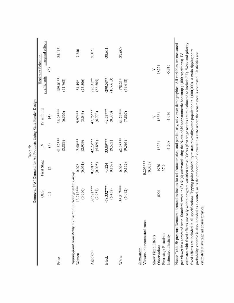
coef

ficie

nts

mar

gina

l effe

cts

(1)

(2)

(3)

(4)

Pric

e-4

1.52

***

-36.

98**

*-1

89.0

1**

-25.

115

(8.8

83)

(6.3

66)

(71.

768)

Tipp

ing-

poin

t pro

babi

lity ×

Fra

ctio

n in

Dem

ogra

phic

Gro

upW

omen

13.2

12**

*0.

078

17.5

0***

9.97

***

54.4

9*7.

240

(0.9

90)

(0.0

61)

(2.9

59)

(3.0

43)

(25.

506)

Age

d 65

+32

.521

***

0.29

1**

42.2

3***

47.7

5***

226.

31**

30.0

71(2

.957

)(0

.095

)(5

.891

)(6

.773

)(8

6.50

5)

Bla

ck-6

8.33

2***

-0.2

2433

.89*

**-4

2.53

***

-290

.58*

*-3

8.61

1(6

.458

)(0

.167

)(9

.521

)(8

.370

)(1

07.6

13)

Whi

te-5

6.81

7***

0.09

8-6

2.98

***

-64.

74**

*-1

78.2

1*-2

3.68

0(6

.092

)(0

.152

)(9

.561

)(7

.867

)(6

9.61

8)

Inst

rum

ent

Vie

wer

s in

unco

ntes

ted

stat

es0.

203*

**(0

.033

)Sh

ow F

ixed

Effe

cts

YO

bser

vatio

ns18

221

1976

1822

118

221

Firs

t-sta

ge F

-sta

tistic

37.9

Estim

ated

Ela

stic

ity-1

.208

-1.0

76

Y18

221

Not

es: T

able

5b

pres

ents

Dem

ocra

t dem

and

estim

ates

for a

d ch

arac

teris

tics,

and

parti

cula

rly, a

d vi

ewer

dem

ogra

phic

s. A

ll va

riabl

es a

re m

easu

red

per v

iew

er in

a c

onte

sted

stat

e. S

tand

ard

erro

rs in

(3) &

(4) e

stim

ated

usi

ng th

e N

-out

-of-

N n

onpa

ram

etric

boo

tstra

p (1

,000

repe

titio

ns).

IV

estim

ates

with

fixe

d ef

fect

s use

onl

y w

ithin

-pro

gram

var

iatio

n ac

ross

DM

As (

first

stag

e re

sults

are

re-e

stim

ated

to in

clud

e FE

). W

eek

and

prio

rity

fixed

effe

cts a

re in

clud

ed in

all

spec

ifica

tions

. Tip

ping

poi

nt p

roba

bilit

y =

stat

e pi

vota

lity/

stat

e po

pula

tion

in 1

,000

,000

s. A

mai

n tip

ping

poi

nt

prob

abili

ty v

aria

ble

is a

lso

incl

uded

as a

con

trol,

as is

the

prop

ortio

n of

vie

wer

s in

a st

ate

whe

re th

e se

nate

race

is c

onte

sted

. Ela

stic

ities

are

es

timat

ed a

t ave

rage

ad

char

acte

ristic

s.

-5.8

15

Tabl

e 5b

Dem

ocra

t PA

C D

eman

d fo

r Ad

Prod

ucts

Usi

ng S

tate

Bor

der D

esig

n

(5)

Hec

kman

Sel

ectio

n IV

with

FE

IVFi

rst S

tage

OLS

(1)

(2)

(3)

(4)

(5)

(6)

Estim

ated

Util

ity

0.62

3***

0.53

4***

0.59

8***

0.67

6***

0.47

8***

0.47

2***

(0.0

20)

(0.0

36)

(0.0

49)

(0.0

31)

(0.0

59)

(0.0

59)

Cos

t0.

210*

**0.

208*

**0.

374*

**0.

374*

**(0

.050

)(0

.050

)(0

.082

)(0

.082

)

Con

stan

t0.

000

-0.0

02**

*-0

.004

***

-0.0

01**

*-0

.001

***

-0.0

01(0

.000

)(0

.000

)(0

.001

)(0

.000

)(0

.001

)(0

.001

)

YY

Obs

erva

tions

5204

2049

2049

1976

943

943

Tabl

e 6

Test

s of S

tatio

n O

ptim

izat

ion

Not

es: T

able

6 sh

ows t

he re

latio

nshi

p be

twee

n es

timat

ed P

AC

will

ingn

ess-

to-p

ay fo

r ad

spot

s and

pur

chas

e pr

ices

. Und

er th

e nu

ll hy

poth

esis

that

stat

ions

are

sing

le-p

rodu

ct m

onop

olis

ts, t

he c

oeffi

cien

t on

estim

ated

util

ity is

0.5

. All

varia

ble

are

mea

sure

d pe

r co

ntes

ted

view

er. C

ost i

s the

low

est u

nit r

ate

paid

by

cam

paig

ns fo

r an

indi

stin

guis

habl

e pr

oduc

t dur

ing

the

60-d

ay w

indo

w b

efor

e th

e ge

nera

l ele

ctio

n; th

ere

are

few

er o

bser

vatio

ns in

regr

essi

ons i

nclu

ding

cos

t sin

ce L

UR

dat

a is

ava

ilabl

e on

ly if

a c

ampa

ign

purc

hase

s. H

eter

oske

dast

icity

-rob

ust s

tand

ard

erro

rs in

par

enth

eses

. Coe

ffici

ents

are

stat

istic

ally

sign

ifica

nt a

t the

* .0

5, *

* .0

1 an

d, *

** .0

01 le

vel.

Pric

e Pa

id b

y R

epub

lican

PA

Cs

Pric

e Pa

id b

y D

emoc

rat P

AC

s

Expe

cted

U

nobs

erve

d U

tility

Pric

e Pa

id v

s Est

imat

ed U

tility

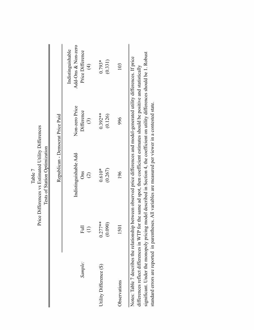
Sample:

Full

Indi

stin

guis

habl

e Add

-O

nsN

on-z

ero

Pric

e D

iffer

ence

Indi

stin

guis

habl

e

Add

-Ons

& N

on-z

ero

Pric

e D

iffer

ence

(1)

(2)

(3)

(4)

Util

ity D

iffer

ence

($)

0.27

7**

0.61

0*0.

392*

*0.

793*

(0.0

90)

(0.2

67)

(0.1

26)

(0.3

31)

Obs

erva

tions

1501

196

996

103

Tabl

e 7

Test

s of S

tatio

n O

ptim

izat

ion

Not

es: T

able

7 d

escr

ibes

the

rela

tions

hip

betw

een

obse

rved

pric

e di

ffere

nces

and

mod

el-g

ener

ated

util

ity d

iffer

ence

s. If

pric

e di

ffere

nces

refle

ct d

iffer

ence

s in

WTP

for t

he sa

me

ad sp

ot, t

hen

coef

ficie

nt e

stim

ates

shou

ld b

e po

sitiv

e an

d st

atis

tical

ly

sign

ifica

nt. U

nder

the

mon

opol

y pr

icin

g m

odel

des

crib

ed in

Sec

tion

4, th

e co

effic

ient

on

utili

ty d

iffer

ence

s sho

uld

be 1

. Rob

ust

stan

dard

err

ors a

re re

porte

d in

par

enth

eses

. All

varia

bles

are

mea

sure

d pe

r vie

wer

in a

con

test

ed st

ate.

Rep

ublic

an -

Dem

ocra

t Pric

e Pa

id

Pric

e D

iffer

ence

s vs E

stim

ated

Util

ity D

iffer

ence

s

Republican PACS Number of Ads Democrat PACS Number of Ads

60 Plus Association 625 AFL-CIO 27Special Operations OPSEC Education Fund 198 AFSCME 1,167American Action Network 5,832 Alliance for a Better MN 202American Chemimstry Council 74 Committee for Justice & Fairness 249American Energy Alliance 21 DNC 206American Future Fund 1,164 Florida Democratic Party 65American Unity PAC 9 Independence USA PAC 167Americans for Job Security 1,769 League of Conservation Voters 486Americans for Prosperity 3,200 MN United for All Families 721Americans for Tax Reform 37 MoveOn.org 38Campaign for American Values 54 Moving Ohio Forward 169Center for Individual Freedom 101 National Education Association 427Checks and Balances for Economic Growth 26 Patriot Majority PAC 574Club for Growth Action Committee 279 Planned Parenthood 415American Crossroads/Crossroads GPS 16,296 Priorities USA 3,306Emergency Committee for Israel 16 SEIU 904Ending Spending PAC 118 Women Vote! 203Freedom Fund 74 Total 9326Freedom PAC 68Government Integrity Fund 170Judicial Crisis Network 54Live Free or Die PAC 290National Association of Manufacturers 197National Federation of Independent Business 262National Republican Trust 65National Rifle Association 142Now or Never PAC 119Republican Jewish Coalition 1,017Republican Party of Florida 150Restore Our Future 5,529RNC 5,806Securing Our Safety 46SuperPAC for America 31US Chamber of Commerce 1,020Women Speak Out PAC 22Young Guns Action Fund 397Total 45278

Table A1Political Action Committee Classification

Notes: PACs are classified as Republican or Democrat based on the classification (conservative or liberal) at OpenSecrets.org, a website maintained by the Center for Responsive Politics.

Criteria Number Dropped Percent of Raw SampleMissing show name 1,048 0.46

Aired before 08/01/2012 7,020 3.09

Longer or shorter than 30 seconds 9,406 4.14

Non-presidential PAC 37,031 16.29

PAC purchased < 20 spots 398 0.18

No clear party affiliation 15,201 6.69

Station with single-party advertising 14,716 6.47

Station without presidential advertising 7,835 3.45

Total eliminated 92,655

Table A2Selection of Ads from the Online FCC Database

Notes: Table A2 describes how I refine the raw data for demand estimation in section 3. Shows that have no identifiable name cannot be matched to viewership data, so they are excluded from the demand analysis. Shows airing before August 1, 2012 are excluded because stations are not required to post invoices predating August, 2 2012; those that choose to may be a selected sample. I do not consider sales of airtime that are longer or shorter than the standard 30 second spot (e.g. some of these are zeros, indicating time was not sold after all). The analysis also excludes purchases by very small PACs or PACs with no clear party affiliation. Stations with single-party advertising or without campaign advertising are excluded as these suggest purchasing for other races. 134,671 observations remain in the sample.

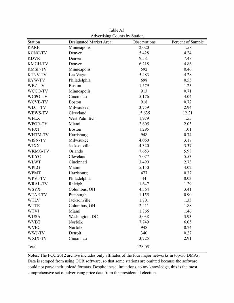
Station Designated Market Area Observations Percent of SampleKARE Minneapolis 2,020 1.58KCNC-TV Denver 5,428 4.24KDVR Denver 9,581 7.48KMGH-TV Denver 6,218 4.86KMSP-TV Minneapolis 592 0.46KTNV-TV Las Vegas 5,483 4.28KYW-TV Philadelphia 698 0.55WBZ-TV Boston 1,579 1.23WCCO-TV Minneapolis 913 0.71WCPO-TV Cincinnati 5,176 4.04WCVB-TV Boston 918 0.72WDJT-TV Milwaukee 3,759 2.94WEWS-TV Cleveland 15,635 12.21WFLX West Palm Bch 1,979 1.55WFOR-TV Miami 2,605 2.03WFXT Boston 1,295 1.01WHTM-TV Harrisburg 948 0.74WISN-TV Milwaukee 4,060 3.17WJXX Jacksonville 4,320 3.37WKMG-TV Orlando 7,653 5.98WKYC Cleveland 7,077 5.53WLWT Cincinnati 3,499 2.73WPLG Miami 5,150 4.02WPMT Harrisburg 477 0.37WPVI-TV Philadelphia 44 0.03WRAL-TV Raleigh 1,647 1.29WSYX Columbus, OH 4,364 3.41WTAE-TV Pittsburgh 1,155 0.90WTLV Jacksonville 1,701 1.33WTTE Columbus, OH 2,411 1.88WTVJ Miami 1,866 1.46WUSA Washington, DC 5,038 3.93WVBT Norfolk 7,749 6.05WVEC Norfolk 948 0.74WWJ-TV Detroit 340 0.27WXIX-TV Cincinnati 3,725 2.91

Total 128,051

Table A3 Advertising Counts by Station

Notes: The FCC 2012 archive includes only affiliates of the four major networks in top-50 DMAs. Data is scraped from using OCR software, so that some stations are omitted because the software could not parse their upload formats. Despite these limitations, to my knowledge, this is the most comprehensive set of advertising price data from the presidential election.

Price Discrimination across Political Action Committees ...

Documents