Price Commitments with Strategic Consumers: Why it can be Optimal to Discount More Frequently ... Than Optimal Gérard P. Cachon and Pnina Feldman * July 18, 2013, revised April 30, 2014; October 16, 2014; January 4, 2015 Abstract In many markets consumers incur search costs and firms choose a long-run pricing strategy that determines how they respond to market conditions. A pricing strategy may involve com- mitments to take actions that do not optimize short-term revenue given the information the firm learns about demand. For example, as already suggested in the literature, the firm could commit to a single price no matter whether demand is strong or weak. We introduce a new strategy - charge a “high” price only if demand is indeed “high”, otherwise offer a discount. This strategy discounts more frequently than would maximize revenue conditional on demand. Nevertheless, the frequent discounts attract consumers. We show that (i) the discount-frequently strategy is optimal (whether capacity is adjustable or not), (ii) discount-frequently is often much better than other pricing strategies, especially if no price commitment is made and (iii) “overbuying” capacity (e.g., inventory) to attract consumers (by signaling availability and the likelihood of discounts) is a poor strategy. Contrary to some recommendations in the literature to limit markdowns and to purchase ample capacity, our results provide support for a strategy that embraces frequent discounts and moderate capacity. * Cachon: The Wharton School, University of Pennsylvania, [email protected]; Feldman: Haas School of Business, University of California, Berkeley, [email protected]. For their helpful comments, the authors thank seminar participants at Santa Clara University, Tel Aviv University, UC Davis, University of Pennsylvania, Northwestern, University of Utah, NYU, Stanford, ESMT, LBS, UC Berkeley, USC, Georgetown, University of Chicago, Washington University at St. Louis, Technion and UC Irvine. 1

Welcome message from author
This document is posted to help you gain knowledge. Please leave a comment to let me know what you think about it! Share it to your friends and learn new things together.
Transcript
Price Commitments with Strategic Consumers:
Why it can be Optimal to Discount More Frequently ... Than
Optimal
Gérard P. Cachon and Pnina Feldman∗
July 18, 2013, revised April 30, 2014; October 16, 2014; January 4, 2015
Abstract
In many markets consumers incur search costs and firms choose a long-run pricing strategy
that determines how they respond to market conditions. A pricing strategy may involve com-
mitments to take actions that do not optimize short-term revenue given the information the firm
learns about demand. For example, as already suggested in the literature, the firm could commit
to a single price no matter whether demand is strong or weak. We introduce a new strategy -
charge a “high” price only if demand is indeed “high”, otherwise offer a discount. This strategy
discounts more frequently than would maximize revenue conditional on demand. Nevertheless,
the frequent discounts attract consumers. We show that (i) the discount-frequently strategy is
optimal (whether capacity is adjustable or not), (ii) discount-frequently is often much better
than other pricing strategies, especially if no price commitment is made and (iii) “overbuying”
capacity (e.g., inventory) to attract consumers (by signaling availability and the likelihood of
discounts) is a poor strategy. Contrary to some recommendations in the literature to limit
markdowns and to purchase ample capacity, our results provide support for a strategy that
embraces frequent discounts and moderate capacity.
∗Cachon: The Wharton School, University of Pennsylvania, [email protected]; Feldman: Haas Schoolof Business, University of California, Berkeley, [email protected]. For their helpful comments, the authorsthank seminar participants at Santa Clara University, Tel Aviv University, UC Davis, University of Pennsylvania,Northwestern, University of Utah, NYU, Stanford, ESMT, LBS, UC Berkeley, USC, Georgetown, University ofChicago, Washington University at St. Louis, Technion and UC Irvine.
1
1 Introduction
In many markets consumers incur costs to search/visit a firm, so they search only if it is worth the
effort. In particular, consumers care about (1) what price they pay and (2) do they get a unit. A
great price does no good for an item that is out of stock or a service that cannot be offered (e.g., no
appointments or seats available). And availability isn’t useful if the price is too high. So in these
environments the firm needs to attract consumers with a good deal (price and availability). The
firm can do this with two levers: a pricing strategy and a capacity choice.
A pricing strategy communicates to consumers how the firm behaves. It often involves commit-
ments to act in certain ways that incur some cost to the firm in the short term. For example, a firm
often has better information about overall demand for a specific product or service than consumers
do. A clothing retailer may know that a dress is more popular than usual or a movie theater may
learn that the latest movie isn’t pulling in audiences as was expected. The dress retailer may be
tempted to raise its price (or not discount it), knowing that it can sell all dresses even at a higher
price. The theater may be tempted to drop its price in an effort to attract bargain hunters. In either
case, failing to make the price adjustment in response to the firm’s updated information is costly
in the short term because changing the price can increase revenue conditional on what the firm
knows, as has been shown in many settings with non-strategic consumers (i.e., consumers whose
search decisions do not depend on the firm’s pricing or capacity choices): e.g., Gallego and van
Ryzin (1994), Talluri and van Ryzin (2004), Elmaghraby and Keskinocak (2003).
This paper studies a model with two time horizons. In the long term the firm, armed with an
uncertain demand forecast, chooses a pricing strategy and possibly a capacity. In the short term
the firm learns useful information about demand and then chooses a price that is consistent with
the adopted pricing strategy. We consider three strategies. With the no-commitment strategy, the
firm charges a price that maximizes revenue conditional on observed demand - if demand is “high”,
the firm charges a high list price, leaving consumers with no residual value, whereas if demand is
“low”, the firm charges a discounted price to ensure that all inventory is sold. With a static-pricing
strategy, the firm commits to a single price no matter what it learns about demand. While a static-
pricing strategy does not allow a firm to exploit new information, it has been found that committing
to a fixed price (or set of prices) can help to reduce the propensity of consumers to strategically
2

wait for discounts (e.g., Besanko and Winston (1990), Aviv and Pazgal (2008)).
We introduce a third strategy, called discount frequently, in which the firm charges either the
high (not discounted) list price or a discounted price, just as in the no-commitment strategy. The
commitment with this policy is with the frequency the firm chooses to discount - in some cases, the
firm discounts off the list price even if it is not in the interest of the firm to discount conditional
on what it observes about demand. With the discount-frequently strategy, a consumer knows that
sometimes she doesn’t get a good deal (the price is high), but the firm nevertheless offers a discount
often enough to justify the effort to visit the firm. For example, given demand, the firm may be
indifferent between selling a portion of its capacity at the high price or discounting to sell all of
its capacity. In those cases, the firm chooses to discount - it loses nothing but makes customers
happier. It also chooses to discount in some cases in which it prefers the higher price. While this is
costly (again, conditional on demand) this commitment attracts more consumers to the firm, which
is clearly beneficial.
For a fixed capacity, we find that (i) the static-pricing strategy can perform well, and in many
cases much better than the no-commitment strategy, (ii) but the discount-frequently strategy is
optimal among all possible strategies. Thus, the best strategy is to charge both high and low prices,
but also to avoid the temptation to maximize the short term (by not offering a discount often enough)
at the expense of long-term profitability. Interestingly, given the same potential demand and the
same capacity, a firm implementing the no-commitment strategy discounts with the same actual
frequency as the firm that implements the discount-frequently strategy. The difference is that the
discount-frequently firm attracts a higher fraction of potential demand, which makes the discount-
frequently strategy more profitable. A naive manager may conclude that a discount-frequently firm
is discounting too frequently given the demand it receives, not recognizing that the firm receives that
demand precisely because it maintains the same frequency of discounting as the no-commitment
firm. However, this can be a costly conclusion - we find that the short term profit gain from avoiding
discounts is generally considerably less than the loss in long-run profit if the firm loses its reputation
for discounting frequently.
If the firm can choose its capacity, then it can also use capacity as a “carrot” to attract consumers.
Dana and Petruzzi (2001) show that if consumers care about availability - they don’t like incurring
the cost to search the firm only to learn that they cannot purchase the good or service - then
3
the firm should invest in more capacity than it would if consumers were non-strategic. (Gaur and
Park (2007) find an analogous result in a model with consumer learning and multiple firms.) The
additional capacity is meant to reassure consumers that the product will be available for them so
they become more likely to search the firm - the firm cannot sell to a customer that does not visit.
Similarly, adding capacity increases the likelihood that a clearance sale is justified, thereby exciting
consumers with the greater prospect of a good deal. However, Dana and Petruzzi (2001) did not
consider the possibility that the firm could choose its pricing strategy, in particular the frequency
of clearance sales to help draw consumers. We find that it is ineffective to only use excess capacity
to attract consumers. For example, the firm that is unable or unwilling to make price commitments
to attract consumers purchases much more capacity and earns substantially lower profit than the
firm that makes price commitments. As with a fixed capacity, the discount-frequently strategy is
optimal. In fact, when capacity is expensive, discount frequently is the only strategy that makes a
positive profit.
2 Related Literature
We are not the first to study price commitments even though we introduce a novel type of price
commitment. A number of authors consider models in which consumers decide whether to purchase
at the current price or to wait to purchase at a future price (e.g., Besanko and Winston (1990), Aviv
and Pazgal (2008), Liu and van Ryzin (2008), Cachon and Swinney (2009), Feng and Gallego (1995),
Su and Zhang (2009); Cachon and Swinney (2011); Swinney (2011); Ovchinnikov and Milner (2012);
Swinney (2013); Whang (2014)). To combat this strategic behavior, it has been suggested that a
firm commit to restrict discounts. This commitment is costly because it limits the firm’s ability
to react to updated demand information. However, a price commitment can detract consumers
from strategically waiting for a discount. In our model consumers are offered a single price, so they
do not consider whether to “buy now or wait for the discount”. Hence, our motivation for price
commitments is exclusively to attract consumers rather than to prevent strategic waiting.
A critical feature of our model is that consumers incur search costs - consumers choose to visit
the firm only if they anticipate that the reward for doing so (i.e., purchasing a product at a good
price) justifies the effort. Others have incorporated similar search costs, generally in a single firm
4

setting: Baye and Morgan (2001), Dana and Petruzzi (2001), Cil and Lariviere (2012), Alexandrov
and Lariviere (2012) and Su and Zhang (2009). Dana and Petruzzi (2001) have fixed prices and focus
instead on how search costs influence the firm’s capacity choice. Baye and Morgan (2001) studies a
marketplace for price information for which customers may pay to subscribe or, alternatively, incur
search costs to learn the price set by their local firm only. Cil and Lariviere (2012) studies the
allocation of capacity across two market segments and Alexandrov and Lariviere (2012) study why
firms may offer reservations. Prices are exogenously fixed in both of those papers. Su and Zhang
(2009) focus on capacity commitments and availability guarantees.
Pricing and availability is considered in a number of papers that model competition across two or
more firms: e.g., Deneckere and Peck (1995), Bernstein and Fedegruen (2004), Cachon and Harker
(2002), Gaur and Park (2007), and Allon and Fedegruen (2007). These models assume firms choose
a price without the benefit of updated demand information. Several papers empirically document
that consumers do value higher availability: e.g., Masta (2011), and Cachon et al. (2013).
Other papers that compare different pricing schemes when consumers are strategic include single
versus priority pricing (Harris and Raviv (1981)), subscription versus per-use pricing (Barro and
Romer (1987); Cachon and Feldman (2011)), and markdown regimes with and without reservations
(Elmaghraby et al. (2009)). In all of these papers the firm selects its pricing strategy before learning
some updated demand information, whereas in our study we allow the firm to choose a price after
potential demand is observed. Thus, consumers in our model are not sure what is the firm’s price
or the product’s availability before they choose whether to search the firm.
3 Model Description
A single firm with k units of capacity sells to two types of consumers, high types and low types,
all of whom require one unit of capacity to be served and are indistinguishable to the firm. There
is a potential number of X high-value consumers, where X is a non-negative random variable that
is drawn from a cumulative distribution function F (·), probability density function f(·), and mean
µ = E[X]. Let F̄ (·) = 1 − F (·). The high-value consumers have zero “mass” as each is unable to
have any influence on the market individually. They have value vh for the firm’s service. As in Dana
and Petruzzi (2001) (and other papers), high-value consumers must incur a positive cost, c < vh,
5

Table 1. Summary of Consumer Types.
Segment Number Value Search costHigh type X ∼ F (·) vh cLow type ∞ vl 0
to search the firm to purchase the good or service. These search costs include the time and effort
to physically travel to the firm and the mental effort associated with a purchasing decision. They
receive 0 value if they choose not to search. They can implement mixed strategies: let γ ∈ [0, 1] be
the probability that a high-type consumer searches the firm. Mixed strategies have also been used
to describe consumer behavior in the context of joining a service, modeled as a queue (e.g., Edelson
and Hildebrand (1975) and Lariviere and van Mieghem (2004)), paying to have access to a list of
prices from multiple firms (e.g., Baye and Morgan (2001)), and whether to visit a restaurant (e.g.,
Cil and Lariviere (2012)).
There is an ample number of low-value consumers, and each has vl value for the firm’s service.
These consumers have zero (or low) search costs. We assume throughout vl < vh − c: a high-type
consumer who visits the firm generates more value than a low type (net of search cost). If vl > vh−c,
then the firm prefers selling exclusively to low-type consumers, which is not interesting. Table 1
summarizes the consumer types.
The firm seeks to maximize revenue and consumers seek to maximize their net value, the value
of the service minus search costs and the price paid to the firm.
Events can be divided into two periods. In the first, or “long-term”, period the firm chooses
a pricing strategy. The strategy determines how the firm behaves in the second, or “short term”
period. All consumers observe the firm’s pricing strategy. At the start of the second period the
number of high-type consumers, X, is realized. The firm observes X but consumers do not. Next,
the firm chooses a price, p, and at the same time the high-type consumers choose to search the
firm or not (i.e., they select γ). At the end of the short-term period consumers who visit the firm
purchase an item, if available. If there are more than k high-type consumers who want to purchase,
the k units are randomly rationed among them (our allocation rule). While we model the “short
term” period as a single period, results are equivalent to a model that has one “long-term” period
followed by multiple but independent “short-term” periods (hence the names).
We consider three pricing strategies. With the first, called “no commitment”, the firm chooses a
6
price in the short-term period that maximizes revenue conditional on observed demand, X, capacity,
k, and the firm’s expectation of consumer behavior. There is no commitment with this strategy
because the firm is maximizing its short term revenue conditional on all of the information it knows.
The second pricing strategy is called “static pricing” because in the long-term period the firm
commits to charge a single price, ps, in the short-term period. This requires a commitment because
ps may not be the price that maximizes the firm’s revenue in the short-term period. However, by
committing to ps < vh, the firm potentially increases the return a high type receives from search,
thereby increasing the number of high-type consumers who search. Finally, we consider a “discount
frequently” strategy in which the firm chooses the same prices as in the no-commitment strategy (vl
or vh), but chooses the discount price with a higher likelihood (i.e., more frequently) than with the
no-commitment strategy. Hence, the firm sometimes does not maximize revenue in the short-term
period conditional on its information, but this commitment also encourages high types to search
the firm because they expect to receive the discounted price with a higher probability.
There are additional pricing strategies beyond the three we consider. For example, instead of
committing to the frequency of the two focal prices (vl or vh), the firm could commit to always
offer a discount by either choosing to maximize short term revenue with an intermediate price vm,
vl < vm < vh, or the deep discount, vl. (If vm = vh, then this is the no-commitment strategy. If
vm = ps, then this strategy dominates static pricing.) Using the set of scenarios described in our
numerical study (Sections 5 and 6), we find this “discount always” strategy is reasonably effective
when capacity is fixed (it achieves on average 96.9% of the revenue earned with discount frequently),
but less effective when capacity can be chosen (it earns on average only 79% of the profit earned
by discount frequently). (A complete analysis of the discount always policy is available from the
authors.)
There are several important features of our model, which we discuss next.
The firm is able to commit to a pricing strategy. Like Aviv and Pazgal (2008), Liu and van
Ryzin (2008), Elmaghraby et al. (2008), Yin et al. (2009), Liu and Shum (2013) and Whang (2014),
(i) we allow the firm to commit to a pricing strategy that is not always sub-game perfect and
(ii) we presume these commitments are credible. Credibility is generally achieved through repeated
interaction (e.g., Fudenberg and Levine (1989)). Although we consider a model with only one short-
term period, we have in mind a situation in which the firm interacts with consumers over multiple
7

short-term periods (e.g., multiple months or quarters). Consequently, the firm is able to establish
a longrun reputation for how it conducts business. For example, in January 2012, JC Penney, a
large U.S. department store chain, announced a new, simplified pricing strategy that involved far
fewer discounts. However, by the spring of 2013, the company decided that the strategy did not
work and they returned to a more aggressive use of price promotions (Clifford and Rampell (2013)).
Thus, a firm commits to a pricing strategy through advertising and subsequent behavior - consumers
who visited JC Penney after the announcement indeed noticed that they were not promoting as
frequently.
Consumers must incur a search cost before observing availability and price. Search costs asso-
ciated with product availability are likely to be inconsequential only if a consumer knows exactly
which item they want (at the brand/model level) and they have the ability to find availability infor-
mation quickly and accurately. Those conditions are likely to apply only in specialized situations.
It is more common that consumers might not know exactly the item they want, or shop at retailers
that are unable to easily provide accurate availability information. A department store, such as JC
Penney, fits this description - a consumer might know that they want to purchase a blender from
their housewares department, but they don’t know the exact brand and model, and even if they
did, the website (assuming they have easy Internet access) may not provide timely and accurate
inventory information for their local store. (See DeHoratius and Raman (2008) for evidence that
firms struggle to maintain accurate inventory records, even for their own internal use.) It is also
likely that consumers incur significant search costs for price. Again, for the search cost to be in-
consequential, the consumer must know the precise item they intend to purchase, which doesn’t
always apply. But even if that is known, search costs can remain. For example, a search on a
retailer’s website may provide the price of an item at one store near the consumer, but retailers do
not always charge the same price across all stores. To find the full list of prices in the nearby stores
may require calling the individual stores, which is clearly time consuming (i.e., a costly activity).
Finally, Hann and Terwiesch (2003) discover that consumers act as if price search is costly even
when intuition suggests it shouldn’t be, possibly due to cognitive effort or limitations (e.g., Miller
(1956), Roberts and Lattin (1997), Kuksov and Villas-Boas (2010)). In sum, it is likely that in
many markets consumers behave as if searching for price and availability are consequential (i.e.,
costly).
8

Low types have no search costs. In contrast to the high types that are limited in number and
incur search costs, low types are ample and search is inconsequential to them. One interpretation
is that the low-type consumers are bargain hunters who visit the store without the intention to
purchase in the category of interest but nevertheless are willing to make a purchase if they notice a
very good deal (e.g., the price is no more than vl). Alternatively, even if low-type consumers have a
search cost, the qualitative results of the model remain. To explain, as long as their search costs are
sufficiently low, a certain fraction of them will be willing to visit the store (like the high types, they
would make a tradeoff between the cost of visiting and the potential value of visiting). Thus, the
firm would continue to make the tradeoff between pricing “high” to sell only to the high types and
pricing “low” to sell to both types. The firm might not always be able to clear remaining inventory
with the “low” price, but the firm could still generate a considerable sales boost by discounting its
price.
The firm observes demand before selecting its price. The firm may use early season sales to
quickly determine if the product has excess demand or not (e.g., Raman and Fisher (1996), Iyer
and Bergen (1997), Caro and Gallien (2012)). The firm uses this information when it chooses its
price, constrained by its pricing strategy (and capacity) commitments. Although we assume the firm
observes a perfect signal of demand, we suspect our qualitative results continue to hold (though the
analysis becomes more cumbersome) if the firm is imperfectly informed but remains better informed
than consumers - when the firm has more information than consumers, consumers know that the
firm may be tempted to use that information to increase its revenue, and, thus, price-commitments
can still be used to attract more demand
High types receive priority in the allocation rule. This allocation rule is most favorable to the
firm because it encourages high-type consumers to visit the firm (they know that they have priority).
(Su and Zhang (2008) and Tereyagoglu and Veeraraghavan (2012) also adopt this allocation rule.)
Alternatively, as in Cachon and Swinney (2009), high-type and bargain hunting consumers could
form a queue in which every 1/θ customer is a high type until there are no more high types, where
θ ∈ [0, 1]. If θ = 1, high types are given full priority, which is the allocation rule we consider. As θ
decreases, high types are more likely to be rationed. Nevertheless, all our results apply even if the
high-type consumers are not given full priority. (Details available from the authors.)
9

4 Analysis
This section analyzes the three pricing strategies already discussed: no commitment, static pricing,
and discount frequently.
4.1 No-Commitment Pricing
Under the no-commitment strategy, the firm chooses either vh or vl. Given {vl, vh}, the firm can
price at p = vl and earn revenue vlk. Alternatively, it can price at p = vh and earn revenue
vh min {γx, k} . Consequently, the firm chooses p = vl when
x ≤ vlvh
k
γ, (1)
which occurs with probability F (vlk/(vhγ)) and chooses p = vh, otherwise.
The high-type consumers only earn positive utility if the price is vl and they are able to obtain
the unit. In all other cases, consumers get zero surplus. Thus, to find the high-type consumer
surplus from visiting the firm, let ψ be the high-type consumer’s expectation for the probability
that the firm charges vl and he is able to get a unit. A high-type consumer is indifferent between
searching the firm or not if
ψ (vh − vl) = c. (2)
In equilibrium, the belief about the probability ψ must be consistent with the actual probability.
Given the rationing rule, because vl is charged only when γx ≤ vlvhk < k (from (1)), high-type
consumers are guaranteed to get the unit when the price is vl - the firm discounts the product only
when demand is sufficiently low, which means that a unit is available for everyone. They may not
be able to get a unit if the price is vh, but in this case, their surplus is zero either way. Thus,
high-type consumers do not face a rationing risk if their utility from getting a unit is positive.
From (1), the high-type consumer knows that the firm charges a low price when demand is
sufficiently low. From the perspective of a consumer, the probability density function of x is f̃(x) =
xf(x)/µ. (See Deneckere and Peck (1995) for a detailed derivation of the the demand density
conditional on a consumer’s presence in the market, f̃(x).) Therefore, this consumer anticipates
10
that the price is vl with probability
ψ =
vlvh
kγˆ
0
f̃(x)dx =
´ vlvh
kγ
0 xf(x)dx
µ. (3)
Given vl < vh − c, there exists some γ that satisfies (3). A symmetric equilibrium strategy for
high-type consumers is a γ ∈ [0, 1] such that γ is optimal for each customer given that all other
consumers choose γ as their strategy.
Let γ0 be the fraction of consumers who visit the firm in equilibrium under the no-commitment
policy. The following lemma characterizes γ0. (Proofs are in the online supplement.)
Lemma 1. With the no-commitment pricing strategy, the fraction of high-type consumers who visit
the firm in equilibrium, γ0, is unique. Furthermore, γ0 = 1, if
ˆ vlvhk
0xf(x)dx ≥ µc
vh − vl,
Otherwise γ0 is implicitly defined by
(vh − vl)ˆ vl
vh
kγ0
0xf(x)dx = µc. (4)
The firm’s revenue under no-commitment, R0(γ0), is
R0(γ0) = F
(vlvh
k
γo
)vlk + vhγ0
ˆ kγo
vlvh
kγo
xf(x)dx+ F̄
(k
γo
)vhk
= vlk + vhγ0
(S
(k
γo
)− S
(vlvh
k
γo
)). (5)
4.2 Static Pricing
With a static-pricing strategy, the firm commits to a single price, p, before observing demand, so
consumers know that the price will indeed be p before deciding whether or not to search the firm.
All high-value consumers who search the firm receive a net value equal to vh − p− c if they obtain
a unit, and if they do not obtain a unit, their net value is −c. A customer searches the firm if net
11

utility is not negative, i.e., if
φ(vh − p) ≥ c, (6)
where φ is the customer’s expectation for the probability of getting a unit conditional on searching
the firm. The underlying potential demand distribution, X, the high-value customers’ strategy,
γ, and the rationing rule used to allocate scarce capacity determineφ. All else being equal, as γ
increases, more high-type customers search the firm, thereby reducing the chance that any one of
them gets a unit. Consequently, the probability she gets a unit is
φ =
ˆ ∞0
min {γx, k}γx
f̃(x)dx =
ˆ ∞0
min {γx, k}γx
xf(x)
µdx =
Sγx(k)
γµ
=
ˆ ∞0
min {x, k/γ}µ
f(x)dx =S (k/γ)
µ, (7)
where SD(q) = ED [min {D, q}] is the sales function given demand D and S (·) is shorthand for
SX (·) . (Note, SγX(k) = γS(k/γ).) Given a static price, p, a symmetric equilibrium strategy for
high-type consumers is a γ(p) ∈ [0, 1] such that γ(p) is optimal for each consumer given that all
other consumers choose γ(p) as their strategy. If p is low enough, there is an equilibrium in which
all high-type consumers visit the firm, i.e., γ(p) = 1. From (6) and (7), that occurs if
S(k)
µ(vh − p) ≥ c
or
p ≤ vh −µc
S(k)≡ p̄.
If p > p̄, the unique symmetric equilibrium has γ(p) < 1, where γ(p) is the unique solution to
S
(k
γ(p)
)=
µc
vh − p. (8)
12
Using (8), the firm’s revenue function can be written as a function of γ alone. Define Rhs (γ) as the
firm’s revenue function from only high-type consumers:
Rhs (γ) = SγX(k)
(vh −
µc
S (k/γ)
)= γS
(k
γ
)vh − γµc. (9)
The next lemma finds the equilibrium fraction of high-type consumers who search the firm under
static-pricing, γs.
Lemma 2. Define k̃ implicitly as
vh
ˆ k̃
0xf(x)dx = µc.
With static-pricing, the firm’s revenue function from high-type consumers, Rhs (γ(p)), is concave.
Let γs = arg maxRhs (γ). The price charged to the high types is phs . If k ≥ k̃, then γs = 1 and
phs = p̄. Otherwise γs = k/k̃ and
phs = vh −µc
S(k̃) .
Instead of choosing phs and selling only to high-type consumers, the firm also has the option to
choose ps = vl, in which case the firm sells all its capacity and its revenue is psk. Finally, the firm
chooses the static price, ps ∈{phs , vl
}to maximize revenues. When γs < 1, Rhs (γs) = kvhF̄
(k̃).
Thus, under static-pricing, the optimal price is ps = phs when vhF̄ (k/γs) ≥ vl, otherwise ps = vl.
4.3 Discount Frequently
Static pricing commits to charge some price that is sub-optimal once demand is observed. Although
it is costly, it may be done to increase demand from high-type consumers - they do not visit if the
expectation of what they can receive is too low. However, there is another way to make searching
the firm attractive to consumers. Instead of always providing an intermediate discount (as in static
pricing), the firm could commit to provide the deep discount (to vl) more frequently than would be
optimal given the realization of demand. In particular, with the discount-frequently strategy the
firm chooses to price at either vl or vh (the two optimal prices ex-post), but commits to markdown
to vl whenever potential demand is δk/γf or lower and charge vh otherwise, where δ ∈ [vl/vh, 1].
13

This implies that the firm charges vl with probability F (δk/γf ). Under this policy the firm does
not commit to limit its prices - the firm charges the same prices as in the no-commitment strategy.
Rather, it commits to discount often and deeply, thereby encouraging high-type consumers to search.
The following lemma characterizes the fraction of high-type consumers who search the firm under
the discount-frequently strategy.
Lemma 3. With the discount-frequently strategy, the fraction of high-type consumers who visit the
firm in equilibrium, γf , is unique. Furthermore, γf = 1, if
(vh − vl)ˆ δk
0xf(x)dx > µc (10)
Otherwise γf is implicitly defined by
(vh − vl)ˆ δk/γf
0xf(x)dx = µc. (11)
The revenue function is
Rf (δ, γf ) = vlkF (δk/γf ) + γfvh
ˆ k/γf
δk/γf
xf(x)dx+ vhkF̄ (k/γf ).
If the firm chooses δ = vl/vh, then it replicates the no-commitment strategy. (Hence, discount fre-
quently cannot be worse than no commitment.) However, if δ > vl/vh, then the firm discounts more
frequently than would be optimal to maximize revenue conditional on realized demand (i.e., holding
γf fixed), which may entice enough high-type consumers to visit to justify the cost of discounting
even though demand is high enough to keep the price high. The next theorem characterizes the
optimal discount frequency, δ∗, and the corresponding fraction of high-type consumers who visit
given that discount frequency, γ∗f = γf (δ∗).
Theorem 1. Define k̂ implicitly as
(vh − vl)k̂ˆ
0
xf(x)dx = µc (12)
With the discount-frequently strategy, let δ∗ and γ∗f be the optimal discount frequency and the result-
14
ing high-type consumer search probability, respectively:
δ∗ =
1 k ≤ k̂
k̂/k k̂ < k ≤ k̂vh/vl
vl/vh k̂vh/vl < k
γ∗f =
k/k̂ k ≤ k̂
1 k̂ < k ≤ k̂vh/vl
1 k̂vh/vl < k
According to Theorem 1, the actual probability of a discount is F (k̂) when k ≤ k̂vh/vl (and
F (vlk/vh) otherwise), which is exactly the same probability of a discount with the no-commitment
strategy. The difference is that with discount frequently, the firm enjoys higher demand (more high
types choose to search), precisely because the firm maintains frequent discounts even with the higher
demand. For example, when k < k̂, the firm discounts whenever realized high-type demand is less
than capacity - the firm charges the higher price, vh, only when it is able to sell its entire capacity
to high-type consumers. Consequently, unlike with static pricing, the firm always clears its entire
inventory with the best discount-frequently strategy. Hence, it could be named the “everything
must go” strategy.
The firm’s revenue function with the optimal discount-frequently strategy is
R∗f =
k(vlF
(k̂)
+ vhF̄(k̂))
k ≤ k̂
vlkF(k̂)
+ vh´ kk̂ xf(x)dx+ vhkF̄ (k) k̂ < k < k̂vh/vl
vlkF(vlvhk)
+ vh´ kvlvhk xf(x)dx+ vhkF̄ (k) k̂vh/vl ≤ k
Our main result, reported in Theorem 2, is that discount frequently is optimal for the firm consider-
ing all possible policies. This is a strong motivation for the use of the discount-frequently straetegy.
By offering discounts sufficiently often, and in some cases when the firm’s short term demand does
not justify the discount, the firm provides the motivation needed for consumers to visit, thereby
increasing the firm’s demand, which in turn leads to the maximum revenue.
Theorem 2. The discount frequently strategy maximizes the firm’s revenue.
Why is discount frequently optimal? Commitments are made to make searching the firm more
attractive to consumers, but they are also costly to the firm. Thus, the best commitment sub-
stantially improves the attractiveness of the firm relative to its cost. Suppose the firm observes
15
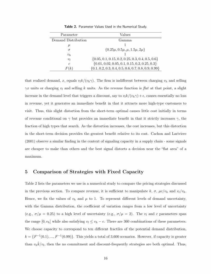
Table 2. Parameter Values Used in the Numerical Study.
Parameter ValuesDemand Distribution Gamma
µ 1σ {0.25µ, 0.5µ, µ, 1.5µ, 2µ}vh 1vl {0.05, 0.1, 0.15, 0.2, 0.25, 0.3, 0.4, 0.5, 0.6}c {0.01, 0.02, 0.05, 0.1, 0.15, 0.2, 0.25, 0.3}
F (k) {0.1, 0.2, 0.3, 0.4, 0.5, 0.6, 0.7, 0.8, 0.9, 0.99}
that realized demand, x, equals vlk/(vhγ). The firm is indifferent between charging vh and selling
γx units or charging vl and selling k units. As the revenue function is flat at that point, a slight
increase in the demand level that triggers a discount, say to vlk/(vhγ) + ε, causes essentially no loss
in revenue, yet it generates an immediate benefit in that it attracts more high-type customers to
visit. Thus, this slight distortion from the short-term optimal causes little cost initially in terms
of revenue conditional on γ but provides an immediate benefit in that it strictly increases γ, the
fraction of high types that search. As the distortion increases, the cost increases, but this distortion
in the short-term decision provides the greatest benefit relative to its cost. Cachon and Lariviere
(2001) observe a similar finding in the context of signaling capacity in a supply chain - some signals
are cheaper to make than others and the best signal distorts a decision near the “flat area” of a
maximum.
5 Comparison of Strategies with Fixed Capacity
Table 2 lists the parameters we use in a numerical study to compare the pricing strategies discussed
in the previous section. To compare revenue, it is sufficient to manipulate k, σ, µc/vh and vl/vh.
Hence, we fix the values of vh and µ to 1. To represent different levels of demand uncertainty,
with the Gamma distribution, the coefficient of variation ranges from a low level of uncertainty
(e.g., σ/µ = 0.25) to a high level of uncertainty (e.g., σ/µ = 2). The vl and c parameters span
the range [0, vh] while also satisfying vl ≤ vh − c. There are 360 combinations of these parameters.
We choose capacity to correspond to ten different fractiles of the potential demand distribution,
k = {F−1(0.1), ..., F−1(0.99)}. This yields a total of 3,600 scenarios. However, if capacity is greater
than vhk̂/vl, then the no commitment and discount-frequently strategies are both optimal. Thus,
16
Figure 1. Comparison of expected revenue with three pricing strategies for one of the considered scenarios(vh = 1, vl = 0.1, c = 0.25, X ∼ Gamma(1, 1))
Figure 2. Revenue Ratios. Diamond = average; the bottom, middle and upper horizontal lines correspond tothe 1st quartile, median and 3rd quartile, respectively; the bottom and top points of the vertical lines are the
minimum and the maximum, respectively.
we remove scenarios that have capacity above this threshold, leaving 3,146 scenarios.
Figure 1 illustrates the revenue achieved with each policy for a representative scenario and a
wide range of capacities. (The 99th percentile of capacity is k = 4.6.) . Although no commitment
performs better than static pricing for very large capacities, for most reasonable capacities, static
pricing performs best and potentially much better. Overall, the figure suggests that the firm sacri-
fices a considerable amount of revenue if it does not make a price commitment (i.e., no commitment
performs poorly). Furthermore, some types of commitments perform much better than others (i.e.,
discount frequently is best). These specific findings extend to our larger sample, as we discuss next.
Figure 2 shows a box-plot of the revenue ratios of the pricing strategies relative to the rev-
enue obtained from discount frequently. As observed in Figure 1, the discount-frequently strategy
17

performs substantially better than no commitment or static pricing. Though both schemes can
approach the discount-frequently strategy in some cases (with maximum ratios of R∗0/R∗f = 1 and
R∗s/R∗f = 99.99%), in most cases they perform poorly in comparison: the average R∗0/R∗f ratio is
63.0% and the average R∗s/R∗f ratio is 88.3%.
The results in Figure 2 emphasize two points. First, failing to make a price commitment can
substantially reduce a firm’s revenue. Second, it is important to make the right price commitment.
In particular, a commitment to a static price is often better than no-commitment, but not effective
relative to discount frequently. Hence, our results do not support a static-pricing strategy. This
runs counter to the results in the literature that suggest a firm should in some cases try to commit
to either not discount, or not discount deeply, or both (e.g. Besanko and Winston (1990), Aviv
and Pazgal (2008), and others). In those papers the motivation for a static-pricing strategy is
to mitigate the negative consequences of consumers strategically waiting for a price discount. As
already mentioned, that motivation is not present in our model, so our results in no way contradict
those findings. Instead, our results provide a counter-argument for the adoption of static pricing.
Specifically, we find that static pricing is not the best strategy for attracting consumers to the firm
when search is costly. Whether it is best to adopt an aggressive discounting strategy (as our model
recommends) or to commit to not offer discounts probably depends on the importance of attracting
consumers to search a firm relative to the desire to prevent consumers from strategically timing their
purchases. In the example of JC Penney, it appears that JC Penney’s decision to limit promotions
prevented consumers from even visiting their stores and the negative effect of this loss in demand
was larger than the benefit of preventing consumers from waiting for sales.
Although discount-frequently maximizes expected profit over all strategies assuming the firm
adheres to its commitment, in the short-term period the firm may have an incentive (depending
on the demand realization) to deviate from its commitment by charging the higher price rather
than a discount. To be specific, based on (5), let R0(γf ), be the firm’s maximum expected revenue
conditional that consumers choose γf as their visit strategy. Hence, deviating from the discount
frequently strategy can increase the firm’s expected revenue by R0(γf ) − R∗f ≥ 0. If the firm and
consumers indeed interacted over only a single period, then the discount frequently commitment
would not be credible. However, in the settings we consider (e.g., a department store), the firm
is likely to interact with consumers over multiple periods, each of which is like our short-term
18

period. In such case, the commitment to follow the discount frequently strategy could be credible
if consumers implement a trigger strategy that penalizes the firm for deviating. With a trigger
strategy, consumers follow the discount-frequently equilibrium until they detect a deviation, at
which point they switch to the no-commitment equilibrium in all subsequent periods. If the trigger
is implemented, the firm’s revenue loss in each period is R∗f −R∗0 ≥ 0. Thus, the discount-frequently
strategy is credible if the profit from deviation, R0(γf )−R∗f , is less than the discounted future loss
of revenue. To determine if this is likely, we evaluate the ratio of the short term gain from deviation
to the single period loss from detection:
R0(γf )−R∗fR∗f −R∗0
.
On average, in our sample, this ratio is 0.51 and in 90% of the scenarios the ratio is 1.0 or lower - on
average the gain in a single period deviation from discount frequently is only 51% of the loss that
is incurred in each period after the trigger is activated. Unless the firm heavily discounts future
revenue, the short term gain is unlikely to be justified by the loss of future revenue, suggesting that
discount frequently can be credible.
The credibility of any pricing strategy also hinges on the ability of consumers to detect a devi-
ation. This cannot be achieved with a single period, but it can be achieved with several periods.
As the required length of the detection period increases, the benefit to the firm from a deviation
increases - R0(γf )− R∗f is earned over multiple periods. Nevertheless, given that the single period
benefit is generally less than even a single period of loss, credibility can be achieved as long as the
firm cares enough about future revenue. See Radnor (1986) and Abreu et al. (1990) for detailed
studies of repeated games with imperfect monitoring. (This issue is also relevant in papers, such as
Liu and van Ryzin (2008), that assume a firm can credibly commit to a fill rate in future periods.)
6 Comparison of Strategies with Capacity Investment
In this section we determine the optimal capacity decisions under each of the pricing strategies and
compare these capacity investments to a “myopic” benchmark that assumes all high types always
search, i.e., γ = 1 for sure. The next theorem characterizes the optimal capacity levels under the
19

Table 3. Optimal capacity levels relative to the myopic consumers optimal capacity. All statistics apply only inthe scenarios in which it is profitable to invest in capacity, i.e., k > 0.
k0/km ks/km kf/km
# of observations with k > 0 662 1254 1800Average 1.90 0.89 1.24
SD 0.77 0.17 0.30Minimum 1.000 0.08 1.00
1st Quartile 1.22 0.84 1.03Median 1.79 0.98 1.13
3rd Quartile 2.43 1.00 1.33Maximum 4.25 1.00 2.94
different policies.
Theorem 3. Let ck be the marginal cost of capacity. Then:
1. Myopic benchmark: The optimal capacity, km, is given implicitly by vhF̄ (k) + vlF(vlkvh
)= ck.
2. No commitment: If ck < c0k = vl + vl
(S(vhk̂vl
)− S(k̂)
)/k̂, then the optimal capacity is
k0 = max{vhk̂/vl, km
}. Otherwise, k0 = 0.
3. Static-pricing: If ck < csk = vhF̄ (k̃), then the optimal capacity, ks, is given implicitly by
F̄ (k) = ck/vh. Otherwise, ks = 0.
4. Discount-frequently: If ck < cfk = vl + (vh − vl)F̄ (k̂), then the optimal capacity is kf =
max {k′′, km}, where k′′ is given implicitly by vhF̄ (k′′) + vlF(k̂)
= ck. Otherwise, kf = 0.
Theorem 4. Assume ck < cfk . The following statements hold:
1. ks < km ≤ kf
2. Let ck = vlF (k̂) + vhF̄(vhk̂vl
). If ck ≤ ck, then km = ko = kf . If ck < ck ≤ c0k, then kf < k0.
To compare the performance of the pricing strategies when capacity can be selected, we again
considered the 360 parameter combinations detailed in Table 2 (excluding k). As ck ∈(vl, c
fk
)is
the interesting range for capacity costs (capacity levels greater than cfk , result in zero profit for any
policy), for each parameter combination we select 5 evenly distributed values from this range, i.e.,
c(i)k = vl + i
(cfk − vl
)/6, i = 1, ..., 5. This yields 1800 scenarios. Table 3 summarizes the ratios of
the optimal capacity relative to the optimal capacity with myopic consumers.
20
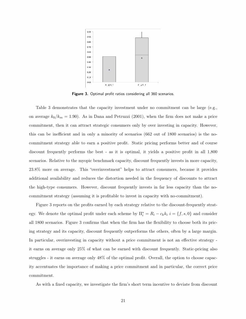
Figure 3. Optimal profit ratios considering all 360 scenarios.
Table 3 demonstrates that the capacity investment under no commitment can be large (e.g.,
on average k0/km = 1.90). As in Dana and Petruzzi (2001), when the firm does not make a price
commitment, then it can attract strategic consumers only by over investing in capacity. However,
this can be inefficient and in only a minority of scenarios (662 out of 1800 scenarios) is the no-
commitment strategy able to earn a positive profit. Static pricing performs better and of course
discount frequently performs the best - as it is optimal, it yields a positive profit in all 1,800
scenarios. Relative to the myopic benchmark capacity, discount frequently invests in more capacity,
23.8% more on average. This “overinvestment” helps to attract consumers, because it provides
additional availability and reduces the distortion needed in the frequency of discounts to attract
the high-type consumers. However, discount frequently invests in far less capacity than the no-
commitment strategy (assuming it is profitable to invest in capacity with no-commitment).
Figure 3 reports on the profits earned by each strategy relative to the discount-frequently strat-
egy. We denote the optimal profit under each scheme by Π∗i = Ri − ckki i = {f, s, 0} and consider
all 1800 scenarios. Figure 3 confirms that when the firm has the flexibility to choose both its pric-
ing strategy and its capacity, discount frequently outperforms the others, often by a large margin.
In particular, overinvesting in capacity without a price commitment is not an effective strategy -
it earns on average only 25% of what can be earned with discount frequently. Static-pricing also
struggles - it earns on average only 48% of the optimal profit. Overall, the option to choose capac-
ity accentuates the importance of making a price commitment and in particular, the correct price
commitment.
As with a fixed capacity, we investigate the firm’s short term incentive to deviate from discount
21

Table 4. Average ratio of short term profit gain, Π̂f −Π∗f , to long-run per period profit loss, Π∗
f −Π0, as a
function of the search cost, c, and the cost of capacity, c(i)k .
c(i)k = vl + i
(cfk − vl
)/6
c i = 1 i = 2 i = 3 i = 4 i = 5
0.01 0.01 0.02 0.04 0.14 0.230.02 0.03 0.05 0.12 0.18 0.350.05 0.11 0.20 0.22 0.30 0.700.10 0.28 0.28 0.34 0.53 1.280.15 0.35 0.37 0.48 0.9 1.890.20 0.44 0.48 0.66 1.10 2.560.25 0.54 0.63 0.87 1.48 3.350.30 0.68 0.81 1.16 1.95 4.33
frequently. Let Π̂f be the single period profit the firm earns if it deviates from discount frequently
even though consumers play the discount frequently equilibirum. On average the ratio of the short
term gain relative to the potential single period loss of profit,
Π̂f −Π∗fΠ∗f −Π∗0
,
is 0.76. This is higher than in the fixed capacity sample (0.51), but still suggests that the gain from
deviating is potentially considerably lower than the loss in future discounted profit. Table 4 reveals
that the consumer’s search cost and the cost of capacity strongly influence this average. When
search is not costly (first three rows), the short term gain from deviating is small compared to the
potential long run loss in profit, and in some cases very small (upper left corner). Given the low
search cost in these scenarios, one might assume that discount frequently does not provide much
of an advantage relative to no commitment. But Table 5 reveals that even with low search costs,
failing to make a price commitment reduces profit by a substantial amount (between 18-100%).
Table 4 also indicates that there are conditions in which credibility might be harder to achieve -
when search is costly and capacity is expensive (lower right corner), the gain from a deviation is
a reasonable amount of the potential loss (up to 4.33 periods). In these cases, credibility requires
the firm to be sufficiently far sighted (which remains possible, just harder). Nevertheless, in these
cases the firm’s bigger problem is that the product is barely profitable (and generally not profitable
with the no-commitment strategy). Overall, even when the firm can choose its capacity, the firm
loses a substantial amount of profit if it either chooses not to make a commitment or if it loses the
22

Table 5. Average ratio of no-commitment profit, Π∗0, to discount frequently profit, Π∗
f .
c(i)k = vl + i
(cfk − vl
)/6
c i = 1 i = 2 i = 3 i = 4 i = 5
0.01 0.82 0.73 0.61 0.43 0.140.02 0.77 0.65 0.51 0.30 0.060.05 0.67 0.51 0.32 0.13 0.000.10 0.54 0.35 0.07 0.04 0.000.15 0.44 0.24 0.10 0.01 0.000.20 0.35 0.17 0.05 0.00 0.000.25 0.28 0.11 0.02 0.00 0.000.30 0.22 0.07 0.00 0.00 0.00
credibility of its commitment.
7 Conclusion
Firms that do not make a price commitment can optimally select a price to respond to available
demand information to maximize revenue. This is the best pricing strategy for the firm if consumers
are not strategic. However, with strategic consumers, even though price commitments are costly to
the firm in the short term, they are useful for attracting demand.
With fixed capacity, we show that a firm can do much better by committing to static-pricing
relative to no price commitment, despite the fact that the commitment reduces the firm’s ability
to match supply with demand. However, static pricing is not the best price commitment strategy.
Discount frequently is the optimal strategy, and it performs substantially better than the other
strategies we study. Thus, while is has been suggested that a static-pricing strategy can mitigate the
negative effects of consumers strategically waiting for end-of-season discounts, we do not recommend
that strategy when it is important to attract consumers to the firm (due to search costs).
When the firm can choose capacity, we show that a firm without a price commitment overinvests
in capacity to attract consumers and earns substantially lower profit, if it can even earn a profit.
As with fixed capacity, the discount-frequently strategy is optimal, and much better than the other
policies.
According to our model, adopting a “simplified pricing policy” or curtailing discounts, as done
by JC Penney in 2012 (Clifford and Rampell (2013)), can backfire considerably. Thus, we conclude
that in the presence of strategic consumers and search costs, (i) price commitments are generally
23
necessary, (ii) the right commitment is discount frequently - the firm should give consumers a
deep discount even if doing so lowers revenue conditional on demand because the higher frequency
of discounts attracts consumers to the firm - and (iii) the firm should not exclusively use excess
capacity as a tool to attract consumers.
Our results theoretically justify the implementation of a discount-frequently strategy. Additional
work could seek to determine if firms currently utilize some form of discount frequently and if
discount frequently is better in practice than alternatives. A firm could be said to be using discount
frequently if they choose deeper discounts than would be optimal given existing inventory and
current unbiased estimates of demand. Although not definitive, further evidence could be provided
via surveys and interviews with managers - managers may intuitively be using a strategy like
discount frequently if they say they are willing to provide discounts at the expense of short term
profits to avoid losing their long-term reputation for offering “good deals” or “competitive prices”.
Finally, JC Penney’s experience provides some support for the effectiveness of discount frequently,
but additional, controlled experiments would offer more direct evidence.
References
Abreu, D., Pearce, D., and Stacchetti, E. (1990). Toward a theory of discounted repeated games with
imperfect monitoring. Econometrica, 58(5):1041–1063.
Alexandrov, A. and Lariviere, M. A. (2012). Are reservations recommended? Manufacturing and Service
Operations Management, 14(2):218–230.
Allon, G. and Fedegruen, A. (2007). Competition in service industries. Operations Research, 55(1):37–55.
Aviv, Y. and Pazgal, A. (2008). Optimal pricing of seasonal products in the presence of forward-looking
consumers. Manufacturing and Service Operations Management, 10(3):339–359.
Barro, R. J. and Romer, P. M. (1987). Ski-lift pricing, with applications to labor and other markets. American
Economic Review, 77(5):875–890.
Baye, M. and Morgan, J. (2001). Information gatekeepers on the internet and teh competitiveness of homo-
geneous product markets. American Economic Review, 91(3):454–474.
Bernstein, F. and Fedegruen, A. (2004). Dynamic inventory and pricing models for competing retailers.
Naval Research Logistics, 51(2):258–274.
24

Besanko, D. and Winston, W. L. (1990). Optimal price skimming by a monopolist facing rational consumers.
Management Science, 36(5):555–567.
Cachon, G. P. and Feldman, P. (2011). Pricing services subject to congestion: Charge per-use fees or sell
subscriptions? Manufacturing and Service Operations Management, 13(2):244–260.
Cachon, G. P., Gallino, S., and Olivares, M. (2013). Does adding inventory increase sales? evidence of a
scarcity effect in u.s. automobile dealerships. Working Paper.
Cachon, G. P. and Harker, P. (2002). Competition and outsourcing with scale economies. Management
Science, 10:1314–1333.
Cachon, G. P. and Lariviere, M. A. (2001). Contracting to assure supply: How to share demand forecasts
in a supply chain. Management Science, 47(5):629–646.
Cachon, G. P. and Swinney, R. (2009). Purchasing, pricing, and quick response in the presence of strategic
consumers. Management Science, 55(3):497–511.
Cachon, G. P. and Swinney, R. (2011). The value of fast fashion: Quick response, enhanced design, and
strategic consumer behavior. Management Science, 57(4):778–795.
Caro, F. and Gallien, J. (2012). Clearance pricing optimization for a fast-fashion retailer. Operations
Research, 60(6):1404–1422.
Cil, E. and Lariviere, M. A. (2012). Saving seats for strategic consumers. Working Paper: Northwestern
University, Evanston.
Clifford, S. and Rampell, C. (2013). Sometimes, we want prices to fool us. New York Times.
Dana, J. D. and Petruzzi, N. C. (2001). Note: The newsvendor model with endogenous demand. Management
Science, 47(11):1488–1497.
DeHoratius, N. and Raman, A. (2008). Inventory record inaccuracy: an empirical analysis. Management
Science, 54(4):627–641.
Deneckere, R. and Peck, J. (1995). Competition over price and service rate when demand is stochastic: A
strategic analysis. The RAND Journal of Economics, 26(1):148–162.
Edelson, N. and Hildebrand, K. (1975). Congestion tolls for poisson queuing processes. Econometrica,
43:81–92.
Elmaghraby, W., Gulcu, A., and Keskinocak, P. (2008). Designing optimal pre announced markdowns in
the presence of rational customers with multiunit demands. Manufacturing and Service Operations
Management, 10(1):126–148.
Elmaghraby, W. and Keskinocak, P. (2003). Dynamic pricing in the presence of inventory considerations.
Management Science, 49(10):1287–1309.
25
Elmaghraby, W., Lippman, S., Tang, C., and Yin, R. (2009). Pre-announced pricing strategies with reser-
vations. Production and Operations Management, 18:381–401.
Feng, Y. and Gallego, G. (1995). Optimal starting times for end-of-season sales and optimal stopping times
for promotional fares. Management Science, 41(8):1371–1391.
Fudenberg, D. and Levine, D. (1989). Reputation and equilibrium selection in games with a patient player.
Econometrica, 57(4):759–778.
Gallego, G. and van Ryzin, G. J. (1994). Optimal dynamic pricing of inventories with stochastic demand
over finite horizons. Management Science, 40(8):999–1020.
Gaur, V. and Park, Y.-H. (2007). Asymmetric consumer learning and inventory competition. Management
Science, 53(2):227–240.
Hann, I.-H. and Terwiesch, C. (2003). Measuring the frictional costs of online transactions: The case of a
name-your-own-price channel. Management Science, 49(11):1563–1579.
Harris, M. and Raviv, A. (1981). A theory of monopoly pricing schemes with demand uncertainty. American
Economic Review, 71(3):347–365.
Iyer, A. V. and Bergen, M. E. (1997). Quick response in manufacturer-retailer channels. Management
Science, 43(4):559–570.
Kuksov, D. and Villas-Boas, M. J. (2010). When more alternatives lead to less choice. Marketing Science,
29(3):507–524.
Lariviere, M. and van Mieghem, J. (2004). Strategically seeking service: how competition can generate
poisson arrivals. MSOM, 6(1):23–40.
Liu, Q. and Shum, S. (2013). Pricing and capacity rationing with customer disappointment aversion. Pro-
duction and Operations Management, 22(5):1269–86.
Liu, Q. and van Ryzin, G. J. (2008). Strategic capacity rationing to induce early purchases. Management
Science, 54(6):1115–1131.
Masta, D. A. (2011). Competition and product quality in the supermarket industry. Quarterly Journal of
Economics, 126(3):1539–1591.
Miller, G. A. (1956). The magical number seven, plus or minus two: Some limits on our capacity for
processing information. The Psychological Review, 63(81-97).
Ovchinnikov, A. and Milner, J. M. (2012). Revenue management with end-of-period discounts in the presence
of customer learning. Production and Operations Management, 21(1):69–84.
Radnor, R. (1986). Repeated partnership games with imperfect monitoring and no discounting. Review of
Economic Studies, 53(1):43–57.
26

Raman, A. and Fisher, M. (1996). Reducing the cost of demand uncertainty through accurate response to
early sales. Operations Research, 44(4):87–99.
Roberts, J. H. and Lattin, J. M. (1997). Review of research and prospects for future insights. Journal of
Marketing Research, 34(3):406–410.
Su, X. and Zhang, F. (2008). Strategic customer behavior, commitment, and supply chain performance.
Management Science, 54(10):1759–1773.
Su, X. and Zhang, F. (2009). On the value of commitment and availability guarantees when selling to
strategic consumers. Management Science, 55(5):713–726.
Swinney, R. (2011). Selling to strategic consumers when product value is uncertain: The value of matching
supply and demand. Management Science, 57(10):1737–1751.
Swinney, R. (2013). Inventory pooling with strategic consumers: Operational and behavioral benefits.
Working Paper.
Talluri, K. T. and van Ryzin, G. J. (2004). The Theory and Practice of Revenue Management. Springer.
Tereyagoglu, N. and Veeraraghavan, S. (2012). Selling to conspicuous consumers: Pricing, production, and
sourcing decisions. Management Science, 58(12):2168–2189.
Whang, S. (2014). Demand uncertainty and the bayesian effect in markdown pricing with strategic customers.
Manufacturing and Service Operations Management. Forthcoming.
Yin, R., Aviv, Y., Pazgal, A., and Tang, C. (2009). Optimal markdown pricing: implications of inventory
display formats in the presence of strategic consumers. Management Science, 55(8):1391–1408.
27
Online Supplement: “Price Commitments with Strategic
Consumers: Why it can be Optimal to Discount More
Frequently...Than Optimal”
Gérard P. Cachon and Pnina Feldman
July 18, 2013, revised April 30, 2014; October 16, 2014; January 4, 2014.
A Proofs
Proof of Lemma 1. Under the “no commitment” policy, the indifferent consumer solves
´ vlvh
kγ
0 xf(x)dx
µ(vh − vl) = c. (1)
As the left-hand-side (LHS) strictly decreases with γ and the right-hand-side (RHS) is constant, there either
exists a unique γ ∈ [0, 1] which solves (1), or, if (vh − vl)´ vlvhk
0 xf(x)dx > µc, there does not exist a γ whichsolves (1), in which case γ0 = 1.
Proof of Lemma 2. First, note that the expected sales function is given by
S
(k
γ
)=
ˆ k/γ
0
xf(x)dx+k
γF̄
(k
γ
)and that
S′(k
γ
)=dS(k/γ)
dγ= − k
γ2F̄
(k
γ
).
Differentiating Rhs (γ) with respect to γ, we get:
ζs(γ) =dRhs (γ)
dγ= vh (S(k/γ) + γS′(k/γ))− µc
= vh
ˆ k/γ
0
xf(x)dx− µc.
Rhs (γ) is concave because ζs(γ) is decreasing in γ. The optimal γs may be 1 (a corner solution) if ζs(1) ≥ 0
or interior, in which case solving the first-order condition ζs(γ) = 0 gets the desired result. Note that γs 6= 0,
because we assume that vh > c.
Proof of Lemma 3. Under the discount-frequently policy, the indifferent consumer solves
(vh − vl)ˆ δk/γf
0
xf(x)dx = µc. (2)
1
As the left-hand-side (LHS) strictly decreases with γ and the right-hand-side (RHS) is constant, there eitherexists a unique γ ∈ [0, 1] which solves (2), or, if
(vh − vl)ˆ δk/γf
0
xf(x)dx > µc,
there does not exist a γ which solves (2), in which case γf = 1.
Proof of Theorem 1. It is useful to think of γf as a function of δ. γf can be rewritten in terms of k̂ bycomparing (2) with the definition of k̂. There are three regimes that specify the relationship:
γf =
δk/k̂ k ≤ k̂δk/k̂ vlvh≤ δ ≤ k̂
k
1 k̂k ≤ δ ≤ 1
k̂ < k ≤ k̂vh/vl
1 k > k̂vh/vl
Whenever γf < 1, (vh − vl)´ δk/γf0
xf(x)dx = µc holds and whenever γf = 1, (vh − vl)´ δk0xf(x)dx > µc
holds. Define δ̂ as follows:
δ̂ =
1 k ≤ k̂k̂k k̂ < k ≤ k̂vh/vlvlvh
k̂vh/vl < k.
Thus, if the firm chooses δ ∈ [vl/vh, δ̂], then γf = δk/k̂. But if the firm chooses δ ∈ [δ̂, 1], then γf = 1. Therevenue function can be written in terms of δ and k̂. As k̂ is fixed, the revenue function can be expressedexclusively in terms of δ (without an implicit function defining another term):
Rf (δ; k̂) =
vlkF(k̂)
+ vh
(δkk̂
) ´ k̂/δk̂
xf(x)dx+ vhkF̄(k̂δ
)vl/vh ≤ δ ≤ δ̂
vlkF (δk) + vh´ kδkxf(x)dx+ vhkF̄ (k) δ̂ < δ ≤ 1.
Differentiate the revenue function:
dRfdδ
=
vh(kk̂
) ´ k̂/δk̂
xf(x)dx vl/vh ≤ δ ≤ δ̂
−vhk2f (δk)(δ − vl
vh
)δ̂ < δ ≤ 1
It is immediately clear that δ > δ̂ is not optimal - in this case the firm is marking down more frequentlythan optimal, but there is no benefit in terms of increased high type demand (they are already all visiting).It is also apparent that it is optimal to choose δ = δ̂.
Proof of Theorem 2. To search for the optimal pricing policy, start by fixing γ, the high-type’s search strat-egy. For a given γ, find a set of prices, one for each possible demand realization, such that the firm’srevenue is maximized and γ is the optimal strategy for high-type consumers. The strategy γ is optimal ifthe high-types’ expected value of search equals their cost of search conditional that γ fraction of high-typeconsumers visit. Next, inspect the set of chosen prices to confirm that the set can be implemented withdiscount-frequently. Finally, if discount-frequently is optimal for any given γ, then it must be the optimalpolicy overall.
2
Begin with some definitions. There exists a threshold demand realization, x̂ = k/γ, such that for eachx < x̂, high-type demand, γx, is strictly less than capacity. For x < x̂, let s(r, x) be the sales function fordemand realization x and price r:
s(r, x) =
k r ≤ vlγx vl < r ≤ vh
(3)
For x ≥ x̂, the firm sells k units for every r ≤ vh.Let P = {p : p : R+ → R+} be the class of price functions that maps each demand realization x to its
price p(x). The firm’s objective is to choose a function p ∈ P that maximizes revenue conditional on a searchconstraint that stipulates that the expected value a high-type receives from search is at least as great as thecost of search:
maxp∈P
R(p) = maxp∈P
ˆ x̂
0
p(x)s(p(x), x)f(x)dx+ k
ˆ ∞x̂
p(x)f(x)dx
s.t.
ˆ x̂
0
(vh − p(x))xf(x)
µdx+
k
γ
ˆ ∞x̂
(vh − p(x))f(x)
µdx ≥ c (4)
The search constraint (4) can be rewritten as:
ˆ x̂
0
p(x)xf(x)dx+k
γ
ˆ ∞x̂
p(x)f(x)dx ≤ g(γ),
whereg(γ) = vhS
(k
γ
)− µc.
Note that g (γ) is independent of the chosen prices. Define the slack in the search constraint as:
g(γ)−ˆ x̂
0
p(x)xf(x)dx− k
γ
ˆ ∞x̂
p(x)f(x)dx.
An increase in any price p (x) has two effects: (i) it increases revenue and (ii) it decreases the slack in theconstraint. Thus, an optimal p (x) can be found by continuously increasing the set of prices so as to maximizethe ratio of the marginal increase in revenue to the marginal decrease in the slack.
Define pl ∈ P as the constant function p(x) = vl ∀x. With this policy the firm generates vlk in revenue,which is a lower bound on the revenue that can be achieved with the optimal policy. Given k, if the searchconstraint is not satisfied with this pricing policy, then γ cannot be the equilibrium search strategy in theoptimal policy (because it does not generate at least vlk in revenue). Thus, it is sufficient to consider valuesof γ such that the search constraint is satisfied with pl: i.e., it must be that γ is sufficiently small so that
(vh − vl)S(k
γ
)≥ µc.
In other words, with the pricing strategy pl, there must be some slack in the search constraint.Starting with pl, we next increase prices for some values of x so as to increase revenue while not violating
the search constraint. For the most part, revenue increases and the slack decreases smoothly in price for eachx, except for the very first increase in the price above vl. The first incremental price increase above vl yieldsa discontinuous decrease in revenue (because all low-type shoppers abandon their purchases). Thus, for allx ≤ x̂, the first incremental price increase is particularly costly - it decreases the slack without increasingrevenue. In fact, the firm generates the same revenue with price vl as it does with price p̂(x) = vlk/(γx).
3
Thus, for all x ≤ x̂, the optimal policy either charges vl, or some price p̂(x) ≤ p(x) ≤ vh. In that range,additional increases in price generate smooth increases in revenue and smooth decreases in the slack. Inparticular, there are two cases to consider:
Case 1: x ≤ x̂, p̂(x) ≤ p(x) ≤ vh. The marginal increase in revenue is ∂R(p)/∂p(x) = γxf(x) and themarginal decrease in the slack with respect to price is xf(x). Thus, the increase in revenue per unit ofdecrease in slack is:
γxf(x)/xf(x) = γ.
Case 2: x̂ < x. The marginal increase in revenue is ∂R(p)/∂p(x) = kf(x) and the marginal decrease inthe slack with respect to price is (k/γ)f(x). Thus, the increase in revenue per unit of decrease is slack is:
kf(x)/(k/γ)f(x) = γ.
To repeat, for all x ≤ x̂, the first incremental price increase above vl actually decreases revenue andslack. Hence, any price increase above vl should first be done in the x̂ < x demand states. In these states,all price increases generate the same constant increase in the ratio of revenue to slack (case 2), the optimalprice is the maximum price so long as the search constraint is satisfied. Therefore, starting with the highestdemand states in the range x̂ < x, increase the price from vl to the maximum price, vh, until either thesearch constraint binds (i.e., all slack is consumed) or the price is increased in all of these demand states.This yields the following price function:
p(x) =
vl x ≤ x̃
vh otherwise
for some x̃ ≥ x̂. If x̃ > x̂, then no slack remains and the above pricing strategy is the optimal solution. Ifx̃ = x̂, then some slack remains in the search constraint and price increases in the x ≤ x̂ can be considered,which is done next.
For x ≤ x̂, an increase in price from vl to p̂(x) increases revenue by (γxp− kvl)f(x) and decreases slackby (p− vl)xf(x). The relative increase in revenue to slack consumed is the ratio:
(γxp− kvl)f(x)
(p− vl)xf(x)=
γ
p− vl
(p− kvl
γx
)which is increasing in x. This implies that, for x ≤ x̂, if the price is increased above vl, then it should beincreased for the highest demand state with the price still at vl. Furthermore, because the marginal increasein revenue to consumed slack equals γ for all price increases above p̂(x) (case 1) and the initial price increasefrom vl to p̂(x) is costly, if a price is increased above p̂(x), then it should be increased all the way to vh.This leads to a pricing policy in which the firm charges either vl or vh, and the search constraint is binding.In particular,
p(x) =
vl x ≤ x′
vh otherwise
where x′ ≤ x̃. The above can be implemented as a discount-frequently policy. Therefore, for a given γ,discount-frequently maximizes revenue, which implies it is an optimal policy.
Proof of Theorem 3. (1) Conditional on observing γ, the firm’s revenue is maximized by discounting to vl
4
when realized high-type demand is less than (vlk)/(vhγ), otherwise the firm charges the high price vh. Ifthe firm follows this policy and all high-type consumers are myopic (i.e., they surely visit the firm), then thefirm’s profit is Πm = vlk+vh
(S(k)− S
(vlkvh
))−ckk. Differentiate Πm with respect to k: η(k) = dΠm/dk =
vlF(vlkvh
)+ vhF̄ (k)− ck. Πm is quasi-concave because η(0) = vh − ck > 0, limk→∞ η(k) = vl − ck < 0 and
η(k) is decreasing when η(k) = 0 (which implies there is a unique k such that η(k) = 0). To demonstratethe latter, note that there is a unique solution to η(k)/vhF̄ (k) = 0 because η(k)/vhF̄ (k) is increasing in k :
η(k)/vhF̄ (k) =vlF
(vlkvh
)− ck
vhF̄ (k)+ 1. (5)
(2) Differentiate the profit function, Π0 = R0 − ckk with respect to k :
dΠ0
dk=
vl + vlk̂
(S(vhk̂vl
)− S(k̂)
)− ck k < vh
vlk̂
vlF(vlkvh
)+ vhF̄ (k)− ck k ≥ vh
vlk̂.
When k < vhvlk̂, Π0(k) is linear and increasing if ck < vl + vl
k̂
(S(vhk̂vl
)− S(k̂)
). If k ≥ vh
vlk̂, Π0(k) is quasi-
concave with a unique solution given by km (see part (1)). Therefore, k0 = max{vhk̂/vl, km
}, if ck < c0k and
0 otherwise. (3) If vhF̄ (k/γs) ≤ vl, the firm charges vl and will choose ks = 0 because ck > 0. Assume thatvhF̄ (k/γs) > vl, so the firm charges ps > vl. Differentiate the profit function, Πs = Rs − ckk with respect tok :
dΠs
dk=
{vhF̄
(k̃)− ck k < k̃
vhF̄ (k)− ck k ≥ k̃.
Observe that for k < k̃ the function is linear and increasing if ck < vhF̄(kγs
). If k ≥ k̃, dΠs(k)/dk
is decreasing and hence Πs(k) is concave, which guarantees a solution exists, is unique and is given byF̄ (k′) = ck/vh if k′ > k̃ and by k̃ otherwise. (4) Differentiate the profit function Πf = Rf − ck with respectto k:
dΠf
dk=
vl + (vh − vl) F̄
(k̂)− ck k ≤ k̂
vlF(k̂)
+ vhF̄ (k)− ck k̂ < k ≤ k̂vh/vl
vlF(vlvhk)
+ vhF̄ (k)− ck k̂vh/vl < k
(6)
From the k < k̂ part, it follows that kf > 0 if and only if ck < cfk . dΠf/dk is continuous and decreasing(strictly decreasing for k ≥ k̂. This implies that there exists a unique capacity level k that maximizes profits.Solving vlF
(k̂)
+ vhF̄ (k)− ck = 0, we get the first candidate k′′. k′′ ≥ k̂ if ck < cfk and comparing it withkm, we get the desired result.
Proof of Theorem 4 . (1) Proof of ks < km: Let τ̃s = vhF̄ (k̃), τs(k) = vhF̄ (k), and τm(k) = vlF(vlkvh
)+
vhF̄ (k). If τ̃s ≤ ck, then km > ks = 0. Suppose now that τ̃s > ck. Since τs(k) < τm(k) ∀k and τ ′s(k) < 0
and τ ′m(k) < 0, it must be that ks < km. Note that ks = F−1 (ck/vh) < k̃ since τ̃s > ck. Proof of km ≤ kf :This immediately follows from Theorem 3. If km ≥ k′′, then kf = km. Otherwise, kf > km. (2) If ck = ck,then km = vhk̂/vl = k0 = k′′ = kf . Thus, for ck ≤ ck we have km = k0 = kf . For ck > ck, k′′ > km and k′′
is decreasing in ck. Thus, kf = k′′ < vhk̂/vl = k0.
5
Related Documents