Price Caps, Oligopoly, and Entry - u.arizona.edusreynold/Price Caps Draft jan31-13.pdf · stant marginal cost, reducing a price cap yields increased total output, consumer welfare,

Price Caps, Oligopoly, and Entry ∗

Stanley S. Reynolds† David Rietzke‡

January 31, 2013

Abstract

This paper investigates the impact of price caps in oligopoly markets

with endogenous entry. In the case of deterministic demand and con-

stant marginal cost, reducing a price cap yields increased total output,

consumer welfare, and total welfare. This result falls in line with classic

results on price caps in monopoly markets, and with results in Earle,

Schmedders and Tatur (2007) and Grimm and Zottl (2010) for oligopoly

markets with a fixed number of firms. However, when demand is de-

terministic and marginal cost is increasing, a welfare improving price

cap may not exist. We also show that a welfare-improving cap may not

exist in the case where demand is stochastic. The fact that a welfare-

improving cap cannot be guaranteed in these two cases points to a sharp

difference in results between an endogenous entry model and oligopoly

models with a fixed number of firms. Finally, we provide sufficient con-

ditions that ensure the existence of a welfare-improving cap in the case

of stochastic demand.

∗We thank Rabah Amir, Veronika Grimm and Gregor Zoettl for helpful comments andsuggestions.†University of Arizona, P.O. Box 210108, Tucson, AZ 85721, [email protected]‡University of Arizona, P.O. Box 210108, Tucson, AZ 85721, [email protected]

1 Introduction

Price ceilings or caps are relevant in many areas including: wholesale electricity

markets, interest on loans and credit, telecommunications services, taxi ser-

vices, and housing in densely populated areas. In electricity markets, price caps

are used in ERCOT (Texas), New England, and PJM (midwest/east coast) re-

gional wholesale markets. Wholesale electricity prices can be extremely volatile

and this volatility can be exacerbated by the exercise of market power (see,

for example, Borenstein, Bushnell and Wolak, 2002). Price caps are one tool

which regulators can use to limit the extent to which firms exercise market

power. The classic justification for the use of price caps is well known in the

case of a monopolist facing constant marginal cost in a perfect-information en-

vironment. A price cap increases marginal revenue in those situations where

it is binding and incentivizes the monopolist to increase output. Total output,

consumer surplus, and total welfare are decreasing in the price cap; as the cap

approaches marginal cost, the welfare optimal (perfectly competitive) level of

output is achieved.

Earle, Schmedders and Tatur (2007) (EST) analyze the impact of price

caps in a Cournot oligopoly setting with constant marginal cost. They show

that the classic monopoly results for price caps carry over to oligopoly when

demand is certain. However, EST show that these results may break down

under demand uncertainty. In particular, they demonstrate that when firms

must make output decisions prior to the realization of demand, total output,

welfare, and consumer surplus may be locally increasing in the price cap.

This result raises into question the effectiveness of price caps as a welfare-

enhancing policy tool. On the other hand, Grimm and Zottl (2010) (GZ)

demonstrate that, within the framework of Cournot oligopoly with uncertain

demand analyzed by EST, there exists an interval of prices such that any price

cap in this interval increases both total market output and welfare compared

to the no-cap case. Thus, while the standard comparative statics results of

price caps do not obtain in EST’s framework, there always exists a welfare-

improving price cap.

1

A limitation of the analyses of EST and GZ is that the number of firms is

assumed to be constant. This assumption may be problematic since imposing a

price cap could reduce expected profit and thereby reduce the number of firms

that choose to enter and compete in the product market. A possible reduction

in the number of firms is precisely what Cottle and Wallace (1983) consider

in their analysis of the imposition of a price ceiling in a perfectly competitive

market subject to demand uncertainty. Our interest is in the impact of price

caps in oligopoly markets in which entry is endogenous.

We modify the analyses of EST and GZ to introduce an initial market entry

stage prior to a second stage of product market competition. Market entry

requires a firm to incur a sunk cost in stage one, prior to stage two product

market competition. The inclusion of a sunk entry cost introduces economies

of scale into the analysis. This would seem to be a natural extension for an

oligopoly analysis. After all, the rationale for an oligopoly market structure

in a homogeneous product market is likely to be based on economies of scale.

Our model of endogenous entry builds on results and insights from Mankiw

and Whinston (1986) (MW) and Amir and Lambson (2000) (AL). MW show

that when total output is increasing in the number of firms but per-firm output

is decreasing in the number of firms (MW call this latter effect the business-

stealing effect), the socially optimal number of firms will be less than the free-

entry number of firms when the number of firms, n is continous. For discrete n

the free entry number of firms may be less than the socially optimal number of

firms, but never by more than one. Intuitively, when a firm chooses to enter, it

does not take into account decreases in per-firm output and profit of the other

active firms. Thus, the social gain from entry may be less than the private

gain to the firm. Amir and Lambson provide a taxonomy of the effects of

entry on total market output in Cournot markets. In particular, they provide

a very general condition under which total equilibrium output is increasing

in the number of firms. Our analysis relies heavily on the approaches and

results in AL. We demonstrate that AL’s condition under which total output

is non-decreasing in the number of firms, is also a sufficient condition for total

output to be non-decreasing in the number of firms when their is a price cap.

2

Our objective is to analyze the impact of price caps in oligopoly markets

in which entry decisions are endogenous. We show that when entry is endoge-

nous, demand is deterministic, and marginal cost is constant, the standard

comparative statics results continue to hold. In this case, a price cap may

result in fewer firms, but the incentive provided by the cap to increase output

overwhelms the incentive to withold output due to a decrease in competition.

It follows that, regardless of the number of firms that enter the market, output

will always increase as the cap is lowered. Welfare gains are realized on two

fronts. First, the cap increases total output. Second, the cap may deter entry,

and in doing so, reduce the total cost associated with entry.

We also consider the case of increasing marginal costs of production. Given

our assumption of a sunk cost of entry, this case implies U-shaped average cost

curves for firms. We show that when demand is deterministic and marginal

cost is increasing, the standard comparative statics results do not hold when

entry is endogenous. In contrast to results in GZ for a fixed number of firms,

it may be the case that any price cap reduces total output and welfare (i.e.,

there does not exist a welfare improving cap). Moreover, we demonstrate that

if marginal cost is increasing sufficiently fast, it may be the case that the

standard comparative statics results are reversed; that is, welfare and output

may be increasing in the price cap.

Finally, we demonstrate that a welfare-improving price cap may not exist

when demand is uncertain and entry is endogenous (for constant marginal

cost). Thus, the results of GZ do not generalize to the case of endogenous

entry. We provide sufficient conditions for existence of a welfare-improving

price cap. These conditions restrict the curvature of inverse demand, which

in turn influences the extent of the business-stealing effect when an additional

firm enters the market. We also consider a version of the model with disposal;

firms do not have to sell the entire quantity they produced, but instead may

choose the amount to sell after demand uncertainty has been resolved. We

show that the sufficient condition for existence of a welfare improving price

cap for the no-disposal model carries over to the model with disposal.

3

2 The Model

We assume there is an arbitrarily large number, N ∈ N, of symmetric potential

market entrants. Our formulation can be viewed as a two-stage game.1 At

the beginning of the first stage, we assume that the N potential entrants are

randomly ordered in a queue and make sequential entry decisions. Each firm’s

entry decision is assumed to be observed by the other firms. We assume that

there is a cost of entry K > 0 which is sunk if a firm enters. If a firm does not

enter it receives a payoff of zero.

In the second stage, each of the n market entrants produces a homogeneous

good. Each firm faces the cost function C : R+ → R+. For the case of

deterministic demand, we will examine both the case of constant marginal

cost and the case of strictly increasing marginal cost. Output decisions are

made simultaneously. The inverse demand function is given by P (Q, θ) which

depends on total output, Q, and a random variable, θ. θ is continuously

distributed according to CDF F with corresponding density f . The support

of θ is bounded and given by Θ ≡ [θ, θ] ⊂ R. Each firm knows the distribution

of θ but must make its output decision prior to its realization. We assume

that a regulator may impose a price cap, denoted p. We make the following

assumptions.

Assumption 1.

(a) P (Q, θ) > 0 for all Q ∈ R+.

(b) P is differentiable in Q with P1(Q, θ) < 02 for each θ.

(c) P is differentiable in θ with P2 > 0 for each Q

(d) limQ→∞ P (Q, θ)− C ′(Q) < 0

1Since entry decisions are made sequentially, this is technically a N+1 stage game. How-ever, for convenience throughout the paper we will refer to the sequence of entry decisionsas the first stage.

2Throughout the paper, for any function, G(x1, x2, · · · , xk), we write Gj(x1, x2, · · · , xk)to indicate the partial derivative of G with respect to xj .

4

(e) maxQ∈R+

E[Q(P (Q, θ)− C(Q))] > K

Assumptions (1a) - (1c) are analogous to the assumptions imposed by

Earle, Schmedders, and Tatur (2007) (EST) (with only differentiability added)

and match the assumptions in Grimm and Zottl (2010) (GZ).3 . Assumption

(1c) is necessary to ensure that equilibrium outputs in the second-stage game

are well defined. Assumption (1d) is not necessary but is included for ease of

exposition.

EST assume that E[P (0, θ)] > c (where c is marginal cost). This assump-

tion ensures that “production is gainful”; that is, given a fixed number, n > 0

of market participants, this assumption ensures that there exist price caps

such that equilibrium market output will be strictly positive. Our assumption

(1e) is a “profitable entry” condition which guarantees that there exist price

caps such that at least one firm enters the market and that equilibrium output

will be strictly positive. We let P denote the set of price caps which induce at

least one market entrant. That is

P ≡{p > 0 | max

Q∈R+

E [Qmin{P (Q, θ), p} − C(Q)] ≥ K

}In this paper we are only concerned with price caps p ∈ P. In the analysis

that follows, we restrict attention to subgame-perfect pure strategy equilibria

and focus on symmetric second-stage equilibria. Finally, for a fixed number of

firms competing in the second-stage sub-game, there generally exist multiple

subgame equilibria. We abstract away from this issue and assume that firms

coordinate on the second-stage symmetric equilibrium with the lowest output

and highest profit per firm (Henceforth, when a second-stage equilibrium is

mentioned this means the subgame equilibrium of the second stage with the

smallest total output).4 For fixed number of firms, both EST and GZ prove

the existence of the studied second-stage equilibrium. So, we take as given the

3Grimm and Zottl assume constant marginal cost and so our assumptions match theirsfor this case. In the case of convex costs, our assumption is analogous.

4It is standard in the literature to examine the properties of both the smallest andlargest equilibria. We focus on the equilibrium with the lowest total output as this is thePareto-preferred equilibrium for all firms who have entered in stage-one.

5

existence of second-stage equilibrium for a fixed set of market entrants.

One other point to note. Imposing a price cap may require demand ra-

tionning. When rationning occurs, we assume rationning is efficient; i.e.,

buyers with the lowest WTPs do not receive output. This is the rationning

assumption used in EST and GZ.

We denote by Q∗n(p), the second-stage equilibrium total output when n

firms enter and the price cap is p. We let q∗n(p) be the per-firm output in this

equilibrium and let π∗n(p) denote each firm’s expected second-stage profit in

this equilibrium. We let Q∞n = Q∗n(∞) be the second-stage equilibrium total

output when n firms enter with no price cap and let q∞n denote the corre-

sponding per-firm output. Let π∞n denote each firm’s expected second-stage

profit in this equilibrium. Firms are risk neutral and make output decisions

to maximize expected profit. That is, each firm i takes the total output of its

rivals, y, as given and chooses q to maximize

π(q, y, p) = E[qmin{P (q + y, θ), p} − C(q)]

After being placed in the queue, firms have an incentive to enter as long

as their expected second-stage equilibrium profit is at least as large as the

cost of entry. We assume that firms whose expected second stage profits are

exactly equal to the cost of entry will choose to enter. As mentioned above,

we restrict attention to subgame-perfect equilibria. For a fixed price cap, p,

subgame perfection in the entry stage (along with the indifference assumption)

implies that the equilibrium number of firms, n∗, is the largest positive integer

less than (or equal to) N such that π∗n∗(p) ≥ K. Clearly, n∗ exists and is

unique. Moreover, for any p ∈ P we also have 1 ≤ n∗ ≤ N , due to Assumption

(1e).

For convenience and clarity, we will define Q∗(p) ≡ Q∗n∗(p), q∗(p) ≡ q∗n∗(p),

and π∗(p) ≡ π∗n∗(p). Similarly, we define Q∞ = Q∞n∗ , q∞ = q∞n∗ , and π∞ = π∞n∗ .

6

3 Deterministic Demand

We begin our analysis by considering a deterministic inverse demand function.

That is, the distribution of θ places unit mass at some particular θ̃ ∈ Θ. In this

section, we will supress the second argument in the inverse demand function

and simply write P (Q). For the case of deterministic demand, we examine

both the case where marginal cost is constant and the case where marginal

cost is strictly increasing. We begin by analyzing the case where marginal cost

is constant, ie for all x ∈ R+, C(x) = cx.

3.1 Constant Marginal Cost

As previously mentioned, for a given number, n ∈ N, of market participants

both EST and GZ prove the existence of a second-stage equilibrium. We there-

fore do not address this issue. Our main result in this section demonstrates

that the classic results on price caps continue to hold when entry is endoge-

nous. We first state three lemmas that are used in the proof of this result; all

proofs are in the Appendix. Before proceeding, we provide one final piece of

notation: for each p ∈ P we define Q̂(p) to equal P−1(p).

Lemma 3.1. For fixed p, extremal (minimal) subgame equilibrium total out-

put, Q∗n(p) is non-decreasing in the number of firms, n. Moreover, extremal

(maximal) equilibrium profit π∗n(p) is non-increasing in the number of firms,

n.

Lemma 3.2. For fixed n, extremal (maximal) subgame equilibrium profit per

firm π∗n(p) is non-decreasing in the price cap p.

Lemma 3.3. The equilibrium number of firms is non-decreasing in the price

cap, p.

Proposition 1. Restrict attention to p ∈ P. Then in equilibrium, total output,

total welfare, and consumer surplus are non-increasing in the price cap.

Proposition 1 is similar to Theorem 1 in EST. However, our model takes

into account the effects of price caps on firm entry decisions. This is an im-

portant consideration, given that Lemma 3.1 ensures that for a fixed price

7

cap, total equilibrium output is non-decreasing in the number of firms. This

fact, along with the fact that a lower price cap may deter entry, suggest that

a reduction in the cap could have the effect of hindering competition and re-

ducing total output. Our result shows that with constant marginal cost and

non-stochastic demand, even if entry is reduced, the incentive for increased

production with a cap will dominate the possible reduction in output due

to less entry. There are two sources of welfare gains. First, total output is

non-increasing in the price cap, so a lower price cap yields either constant or

reduced deadweight loss. Second, a lower price cap may reduce the number of

firms, and thereby decrease the overall cost of firm entry.

An obvious consequence of Proposition 1 is that, with constant marginal

cost, the welfare-maximizing price cap is the lowest cap which induces exactly

one firm to enter. Imposing such a cap both increases output and reduces entry

costs. Since marginal cost is constant, the total cost of production does not

depend on the number of firms that enter. Total production cost is a function

of only total output produced. However, if marginal cost were increasing, the

total production cost associated with a given level of output is decreasing in

the number of firms. Thus, a price cap which increases output and reduces

entry may result in a significant increase in production costs. Finally, note that

with constant marginal cost, a shortage will never arise in equilibrium. This

is driven solely by the fact that p > c for any level of production. However,

if marginal cost is strictly increasing in output, then firms will produce no

more than the quantity at which their marginal cost is equal to the price cap,

and this could result in a shortage in the market. In the next sub-section we

examine the impact of price caps in an environment in which firms have an

increasing marginal cost of production.

3.2 Convex Costs

In this section, we assume that the cost function, C : R+ → R+, is twice

continuously differentiable and for all x ∈ R+, C ′(x) > 0 and C ′′(x) > 0. We

also assume C(0) = 0.

8

Neither EST nor GZ devote significant attention to the issue of increasing

marginal cost. However, it is mentioned in GZ [p. 3, ft. 9] that, when the

number of firms is fixed, under a general convex cost function there always

exists a price cap which strictly increases total output and welfare. Moreover,

EST state [p. 96, ft. 4] that their Theorems 2, 4, and 5 may be generalized

to a convex cost function. These theorems all address the case of stochastic

demand. Neither paper addresses formally whether the classical monotonicity

results hold for a fixed number of firms when marginal cost is increasing.

As in the constant marginal cost case, a decrease in the price cap may

decrease the incentive for firms to withold output (placing upward pressure on

output), but this must be weighed against the fact that each additional unit

of output will be more costly than the next (placing downward pressure on

output). Our first result below demonstrates that when the number of firms

is fixed, there still exists a range of caps under which equilibrium output (the

smallest and largest equilibrium outputs) and associated welfare are monoton-

ically non-increasing in the cap. This range of caps consists of all price caps

above the n-firm competitive equilibrium price. Intuitively, price caps above

this threshold are high enough that marginal cost in equilibrium is strictly

below the price cap for each firm. A slight decrease in the price cap means

the incentive to increase output created by a lower cap outweighs the fact that

marginal cost has increased (since the cap still lies above marginal cost).

When entry is endogenous the welfare impact of a price cap is much less

clear. Suppose, for instance, that inverse demand is log concave. Then for fixed

n equilibrium subgame output is unique for each p and equilibrium output and

profit are continuous in p. If the entry constraint is not binding in the absence

of a price cap (ie π∞ > K), then a price cap slightly less than the equilibrium

price with no cap would leave the equilibrium number of firms unchanged.

Proposition 2 below would then imply that there exists a range of caps under

which equilibrium welfare is non-increasing in the cap. On the other hand,

imposing a price cap may reduce the number of firms; with fewer firms, total

production cost for a given level of output will increase. The overall welfare

impact of imposing a price cap will depend on the balance of its effects on

9

entry, output incentives, and costs.

In this section, we first demonstrate that when the number of firms is

fixed then there exists a range of price caps in which output and welfare are

monotonically non-increasing in the cap; thus extending Theorem 1 in EST

to the case of convex costs. We then provide an example to show that with

strictly convex costs, a welfare improving price cap may fail to exist when

entry is endogenous. In contrast to our result in Proposition 2 for a fixed

number of firms, and GZ’s reference to a similar result, in Proposition 3 we

provide conditions for which output and welfare are strictly increasing in all

binding price caps.

Proposition 2. Fix n ∈ N and define the n-firm competitive price as the

unique price satisfying p̂ = P (nC′−1(p̂)). Then:

(i) The smallest and largest equilibrium outputs are non-increasing in the

price cap for all p > p̂.

(ii) Equilibrium welfare for the smallest and largest equilibrium outputs is

non-increasing in the price capfor all p > p̂.

(iii) A price cap equal to p̂ maximizes welfare. Welfare at this cap is strictly

greater than welfare in the absence of a cap.

In contrast to the result above with a fixed number of firms, we now provide

an example which demonstrates that when entry is endogenous, a welfare-

improving price cap may fail to exist.

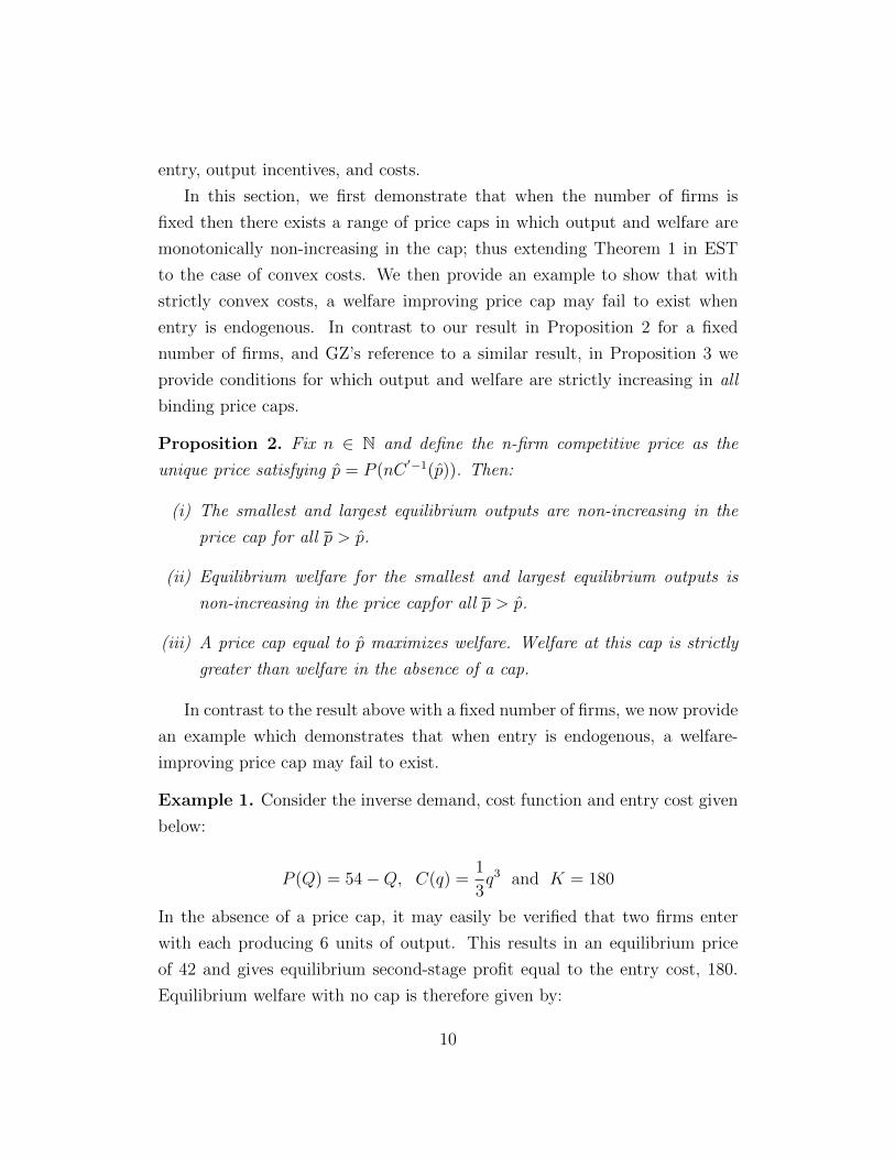
Example 1. Consider the inverse demand, cost function and entry cost given

below:

P (Q) = 54−Q, C(q) =1

3q3 and K = 180

In the absence of a price cap, it may easily be verified that two firms enter

with each producing 6 units of output. This results in an equilibrium price

of 42 and gives equilibrium second-stage profit equal to the entry cost, 180.

Equilibrium welfare with no cap is therefore given by:

10

W nc =

∫ 12

0

(54− t) dt−(

2

3

)63 − 360 = 72

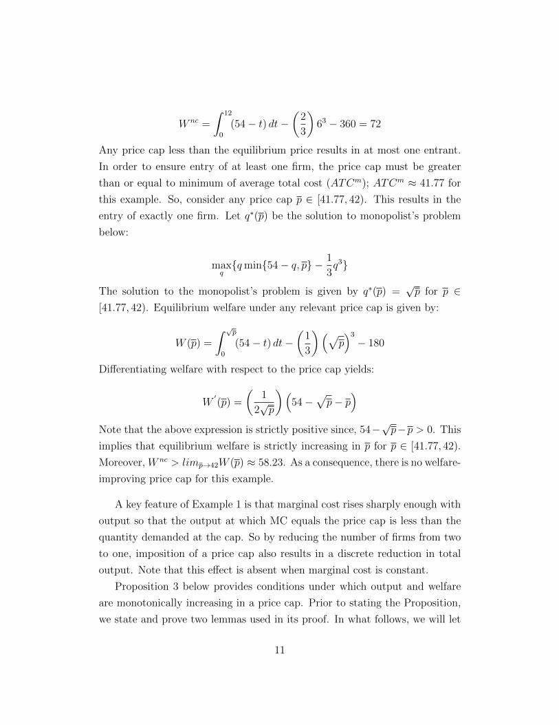
Any price cap less than the equilibrium price results in at most one entrant.

In order to ensure entry of at least one firm, the price cap must be greater

than or equal to minimum of average total cost (ATCm); ATCm ≈ 41.77 for

this example. So, consider any price cap p ∈ [41.77, 42). This results in the

entry of exactly one firm. Let q∗(p) be the solution to monopolist’s problem

below:

maxq{qmin{54− q, p} − 1

3q3}

The solution to the monopolist’s problem is given by q∗(p) =√p for p ∈

[41.77, 42). Equilibrium welfare under any relevant price cap is given by:

W (p) =

∫ √p0

(54− t) dt−(

1

3

)(√p)3− 180

Differentiating welfare with respect to the price cap yields:

W′(p) =

(1

2√p

)(54−

√p− p

)Note that the above expression is strictly positive since, 54−

√p−p > 0. This

implies that equilibrium welfare is strictly increasing in p for p ∈ [41.77, 42).

Moreover, W nc > limp→42W (p) ≈ 58.23. As a consequence, there is no welfare-

improving price cap for this example.

A key feature of Example 1 is that marginal cost rises sharply enough with

output so that the output at which MC equals the price cap is less than the

quantity demanded at the cap. So by reducing the number of firms from two

to one, imposition of a price cap also results in a discrete reduction in total

output. Note that this effect is absent when marginal cost is constant.

Proposition 3 below provides conditions under which output and welfare

are monotonically increasing in a price cap. Prior to stating the Proposition,

we state and prove two lemmas used in its proof. In what follows, we will let

11

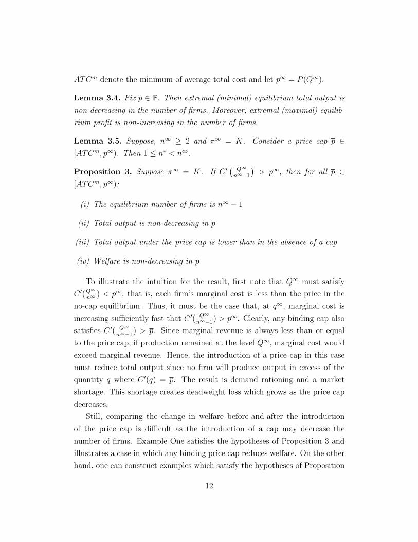
ATCm denote the minimum of average total cost and let p∞ = P (Q∞).

Lemma 3.4. Fix p ∈ P. Then extremal (minimal) equilibrium total output is

non-decreasing in the number of firms. Moreover, extremal (maximal) equilib-

rium profit is non-increasing in the number of firms.

Lemma 3.5. Suppose, n∞ ≥ 2 and π∞ = K. Consider a price cap p ∈[ATCm, p∞). Then 1 ≤ n∗ < n∞.

Proposition 3. Suppose π∞ = K. If C ′(

Q∞

n∞−1

)> p∞, then for all p ∈

[ATCm, p∞):

(i) The equilibrium number of firms is n∞ − 1

(ii) Total output is non-decreasing in p

(iii) Total output under the price cap is lower than in the absence of a cap

(iv) Welfare is non-decreasing in p

To illustrate the intuition for the result, first note that Q∞ must satisfy

C ′(Q∞

n∞) < p∞; that is, each firm’s marginal cost is less than the price in the

no-cap equilibrium. Thus, it must be the case that, at q∞, marginal cost is

increasing sufficiently fast that C ′( Q∞

n∞−1) > p∞. Clearly, any binding cap also

satisfies C ′( Q∞

n∞−1) > p. Since marginal revenue is always less than or equal

to the price cap, if production remained at the level Q∞, marginal cost would

exceed marginal revenue. Hence, the introduction of a price cap in this case

must reduce total output since no firm will produce output in excess of the

quantity q where C ′(q) = p. The result is demand rationing and a market

shortage. This shortage creates deadweight loss which grows as the price cap

decreases.

Still, comparing the change in welfare before-and-after the introduction

of the price cap is difficult as the introduction of a cap may decrease the

number of firms. Example One satisfies the hypotheses of Proposition 3 and

illustrates a case in which any binding price cap reduces welfare. On the other

hand, one can construct examples which satisfy the hypotheses of Proposition

12

3 and for which a welfare-improving price cap exists. Under the hypotheses of

Proposition 3 there are three competing forces which affect welfare. First, a

decrease in the number of firms results in welfare gains associated with entry-

cost savings. Second, as described above, the introduction of a price cap creates

deadweight loss and decreases welfare. Third, the combination of a decrease

in output and a decrease in the number of firms has an ambiguous impact

on firms’ production costs. The effect on welfare depends on the interplay of

these three forces.

4 Stochastic Demand

We now investigate the impact of price caps when demand is stochastic. We

will once again assume that marginal cost is constant and given by c ≥ 0. GZ

demonstrate that under a generic distribution of demand uncertainty, there

exists a range of price caps which strictly increases output and welfare as com-

pared to the case with no cap. We begin this section by providing an example

which demonstrates that this need not be true when entry is endogenous. In

what follows, we let ρ∞ denote the lowest price cap that does not affect prices,

ie ρ∞ = P (Q∞, θ).

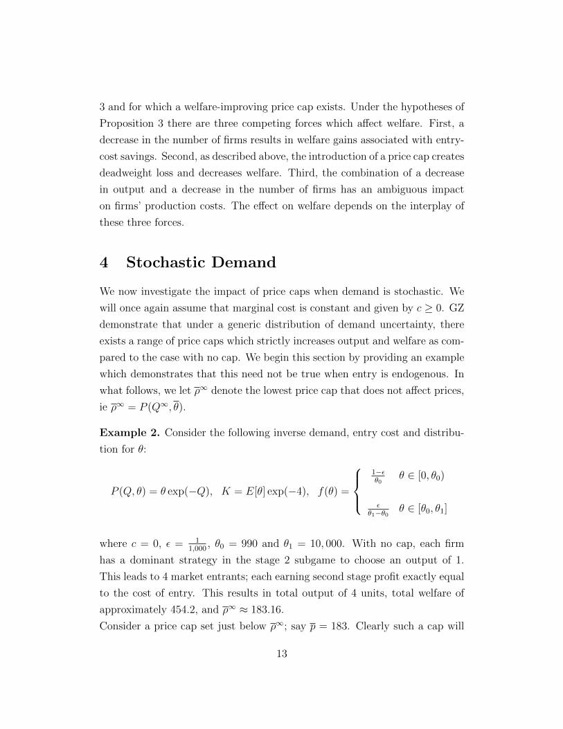
Example 2. Consider the following inverse demand, entry cost and distribu-

tion for θ:

P (Q, θ) = θ exp(−Q), K = E[θ] exp(−4), f(θ) =

1−εθ0

θ ∈ [0, θ0)

εθ1−θ0 θ ∈ [θ0, θ1]

where c = 0, ε = 11,000

, θ0 = 990 and θ1 = 10, 000. With no cap, each firm

has a dominant strategy in the stage 2 subgame to choose an output of 1.

This leads to 4 market entrants; each earning second stage profit exactly equal

to the cost of entry. This results in total output of 4 units, total welfare of

approximately 454.2, and ρ∞ ≈ 183.16.

Consider a price cap set just below ρ∞; say p = 183. Clearly such a cap will

13

deter at least one firm from entering as the entry constraint is binding in the

absence of a cap. Indeed it may be verified that the equilibrium number of

firms under the cap falls to 3 while per-firm output increases to approximately

1.005. Total output falls to 3.015 and welfare decreases to approximately 448.

It may be verified for this example that any binding price cap will deter entry,

reduce total output, and reduce total welfare.

Example 2 demonstrates that when demand is stochastic and entry is en-

dogenous, there need not exist a welfare improving price cap. There are two

important features of this example. First, the exponential inverse demand

function coupled with zero marginal cost implies that firms have a dominant

strategy to choose an output of exactly one unit. Hence, the business-stealing

effect is absent and total output increases linearly in the number of firms.5

Thus, in the absence of a cap, a reduction in the number of firms leads to

a significant decrease in output and welfare. The second feature is the role

and nature of the demand uncertainty. As explained in EST, when demand is

uncertain firms maximize a convex combination of profit when the cap is non-

binding (low demand realizations) and profit when the cap is binding (high

demand realizations). These two scenarios provide conflicting incentives for

firms. When the cap is non-binding, firms have an incentive to withold output

(as in the standard oligopoly model). However, the possibility of a binding cap

(high demand realizations) creates an incentive for firms to increase produc-

tion relative to the case with no cap. In the example above, the distribution of

θ has a long, thin upper tail; there is a possibility that the demand realization

will be extremely high, albeit with a very low probability. A price cap set

just below ρ∞ will therefore bind with very low probability, even if one less

firm competes in stage 2. So, the incentive provided by the cap to increase

production (relative to the no-cap case) is very weak.

The Proposition below provides sufficient conditions on demand that ensure

the existence of a welfare-maximizing cap. Prior to the Proposition, we state

a lemma used in its proof.

5It may be shown that the same result holds for numerical examples with a small marginalcost. In this case the business-stealing effect is present but small.

14

Lemma 4.1. Suppose f(θ) > 0 for all θ ∈ Θ. Then for fixed p, extremal

(minimal) subgame equilibrium total output, Q∗n(p) is non-decreasing in the

number of firms, n. Moreover, extremal (maximal) equilibrium profit π∗n(p) is

non-increasing in the number of firms, n.

Proposition 4. Suppose that inverse demand is additively separable in Q and

θ with P (Q, θ) = θ + p(Q) and that p is twice continuously differentiable and

concave in Q. Moreover, suppose that n∞ ≥ 2. Then there exists a price cap

which increases total welfare.

Proposition 4 provides sufficient conditions for existence of a welfare im-

proving price cap. When demand is concave in output, then the business-

stealing effect is relatively strong. As demonstrated in Mankiw and Whinston

(MW), when the business-stealing effect is present and n is continuous, the

free-entry number of firms entering a market exceeds the socially optimal num-

ber of firms. 6 The proof of Proposition 4 first establishes that, when the entry

constraint is not binding in the absence of a cap, then there is an interval of

prices such that a price cap chosen from this interval will yield the same num-

ber of firms, but higher total output and welfare. This follows directly from

Theorem 1 in GZ. The proof proceeds to show that when the entry constraint

is binding (i.e., zero equilibrium profit in the endogenous entry game) in the

absence of a cap, then a reduction in the number of firms by one will increase

total welfare. Indeed, it may be shown that, in the absence of a cap under the

hypotheses of Proposition 4, the socially optimal number of firms is strictly

less than the free-entry number of firms. The imposition of a price cap in

this case has two welfare-enhancing effects. First, the cap deters entry. As

explained above, in this case entry deterrence (by exactly one firm) is welfare

enhancing. Second, the cap increases total output and welfare relative to what

output and welfare would be in the new entry scenario (ie with one less firm)

in the absence of a cap.

6MW’s result is for a model in which n is a continuous variable, whereas out analysisrestricts n to whole numbers. Nonetheless, we are able to apply the intuition on excess entryfrom MW to prove our result.

15

4.1 Free Disposal

We now examine a variation of the game examined in the previous sections.

This model is a three-stage game. In the first stage, firms sequentially decide

whether to enter or not (again, with each firm’s entry decision observed by

the next). Entry entails some cost K > 0. In the second stage, before θ is

realized, each firm, i, that entered in the first stage simultaneously chooses a

level of capacity, xi ≥ 0 built at constant marginal cost c > 0. In the third

stage, firms first observe θ and then each firm simultaneously chooses a level

of output, 0 ≤ qi ≤ xi, which is produced at zero cost.7 This model has been

analyzed (for a fixed number of firms) by Grimm and Zottl (2006) and has

also been analyzed in the context of price caps by EST and GZ.

This model with free disposal may be interpreted as one in which the firms

that have entered make long run capacity investment decisions prior to ob-

serving the level of demand, and then make output decisions after observing

demand. Under this interpretation, c is the marginal cost of capacity invest-

ment, and the marginal cost of output is constant and normalized to zero.

GZ show that, for a fixed number of firms, in this model there always exists

a price cap which increases total capacity and expected welfare. As with the

proof of Proposition 4, we will demonstrate that in the absence of a price cap,

if the free-entry constraint binds (ie π∞n = K), then welfare is strictly higher

if entry is reduced by one. For this section, we make the following additional

assumptions on P and f :

Assumption 2.

(a) P (Q, θ) ≥ 0 for all Q ∈ R+ and θ ∈ Θ

(b) For all Q and θ such that P (Q, θ) > 0, P is additively separable in Q and

θ with: P (Q, θ) = θ + p(Q)

(c) p is twice continuously differentiable with p′ < 0, and p′′ ≤ 0.

7In the version of the model examined by EST, output is produced at cost δ which maybe positive or negative. Our results continue to hold in this case.

16

(d) θ + p(0) = 0

(e) f(θ) > 0 for all θ ∈ Θ. Moreover, the distribution of θ contains no mass

points.

The assumptions made above are similar to those made in Proposition 4,

but we require that θ + P (0) = 0. This assumption is made in Grimm and

Zottl (2006) and may be viewed as a normalization of the support of θ.

In the absence of a price cap in the third stage, each firm solves:

maxqi

(θ + P (qi + y))qi − cxi such that qi ≤ xi

Let n denote the number of entrants in the first stage in the absence of a price

cap. Under the assumptions made above, there exists a unique symmetric

equilibrium level of capacity for any n ∈ N (Grimm and Zottl, 2006). Denote

by Xn > 0 the total equilibrium capacity and let xn = Xn

ndenote the equilib-

rium capacity per firm. Let Qn(θ) denote the total equilibrium output in the

third stage. Let θ̃(Xn) satisfy:

θ̃(Xn) + p(Xn) + p′(Xn)xn = 0

Assumption 2d above ensures that θ̃(Xn) > θ. Also note that our as-

sumptions are sufficient to ensure θ̃(Xn) is unique for any Xn. Then for

θ ∈ [θ, θ̃(Xn)), it holds that no firm is constrained in equilibrium. In the

unconstrained case, our assumptions above are sufficient to guarantee that a

unique equilibrium exists in the third stage. let Q̃n(θ) denote the total equilib-

rium output in this case and let q̃n(θ) = Q̃n(θ)n

denote the equilibrium per-firm

output. Note that for each θ ∈ [θ, θ̃(Xn)), Q̃n(θ) is given by the first-order

condition:

θ + p(Q̃n(θ)) + p′(Q̃n(θ))q̃n(θ) = 0

So, total equilibrium output in the third stage is given by:

17

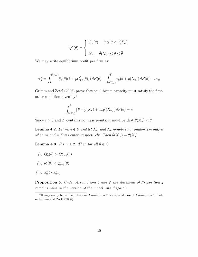
Q∗n(θ) =

Q̃n(θ), θ ≤ θ < θ̃(Xn)

Xn, θ̃(Xn) ≤ θ ≤ θ

We may write equilibrium profit per firm as:

π∗n =

∫ θ̃(Xn)

θ

q̃n(θ)(θ + p(Q̃n(θ))) dF (θ) +

∫ θ

θ̃(Xn)

xn(θ + p(Xn)) dF (θ)− cxn

Grimm and Zottl (2006) prove that equilibrium capacity must satisfy the first-

order condition given by8

∫ θ

θ̃(Xn)

[ θ + p(Xn) + xnp′(Xn) ] dF (θ) = c

Since c > 0 and F contains no mass points, it must be that θ̃(Xn) < θ.

Lemma 4.2. Let m,n ∈ N and let Xm and Xn denote total equilibrium output

when m and n firms enter, respectively. Then θ̃(Xm) = θ̃(Xn).

Lemma 4.3. Fix n ≥ 2. Then for all θ ∈ Θ

(i) Q∗n(θ) > Q∗n−1(θ)

(ii) q∗n(θ) < q∗n−1(θ)

(iii) π∗n > π∗n−1

Proposition 5. Under Assumptions 1 and 2, the statement of Proposition 4

remains valid in the version of the model with disposal.

8It may easily be verified that our Assumption 2 is a special case of Assumption 1 madein Grimm and Zottl (2006)

18

5 Conclusion

This paper has analyzed the welfare impact of price caps, taking into account

the possibility that a price cap may reduce the number of firms that choose

to enter a market. First, we analyzed the welfare impacts of price caps when

there is no uncertainty about demand when firms make their output decisions.

For this case, we showed that when marginal cost is constant, the standard

monotone comparative statics results remain true. That is, output, welfare,

and consumer surplus all increase as the price cap is lowered. We then showed

that when demand is known but marginal cost is strictly increasing, it may

be the case that welfare is lower under any price cap than in the absence of

a cap. We also demonstrated that if marginal cost increases sufficiently fast,

welfare and output may be monotonically increasing in the price cap. Sec-

ond, we analyzed the welfare impacts of price caps when demand is stochastic

and firms must make output decisions prior to the realization of demand. We

showed that, once again the existence of a welfare-improving price cap can-

not be guaranteed. We then provided sufficient conditions on demand under

which a range of welfare-improving price caps will always exist. The sufficient

conditions restrict the curvature of the inverse demand function, which in turn

influences the welfare impact of entry. We also extended this result to an envi-

ronment with free disposal. This type of environment can be viewed as one in

which there is endogenous entry, capacity investment decisions are made prior

to observing demand, and output decisions are made after observing demand.

One limitation of the present analysis is that we restrict attention to Pareto-

dominant symmetric equilibria of stage 2 subgames (except for Proposition 2).

EST and GZ consider extremal equilbria in their analyses, and we plan to ex-

tend our analysis to consider subgame equilibria with both the highest profit

per firm and the lowest profit per firm. A second area for future research

would be to extend our results for free disposal to a model that comes closer

to capturing key features of electricity markets. As noted in our introduc-

tion, regulatory price caps have played an important role in many wholesale

electricity markets. Zottl (2011) examines a modified version of a model with

19

disposal that allows for multiple production technologies. His multiple tech-

nologies model can be interpreted as a model of electricity generation that

allows for baseload, mid-merit, and peaker generation technologies. Firms

make long run investments in capacity for the various technologies, and short

run decisions about production after observing demand shocks. Our interest

is in extending this type of mulitple technologies model to allow endogenous

entry in a setting with a price cap.

20

Appendix

Proof of Lemma 3.1

Proof. Since limq→∞ π(q, y, p) < 0 there exists some M > 0 such that a firm’s

best response is bounded by M . As in Amir and Lambson (2000) (AL), we

can express a firm’s problem as choosing total output, Q given y.

max{π̃(Q, y, p) ≡ (Q− y) min{P (Q), p} − c(Q− y) : y ≤ Q ≤ y +M} (1)

We claim that for any p > c, the maximand in (1) satisfies the single-

crossing property in (Q; y) on the lattice

Φ = {(Q, y) : 0 ≤ y ≤ (n− 1)M, y ≤ Q ≤ y +M}

To see this, let Q′ > Q and y′ > y such that the points (Q′, y′), (Q′, y),

(Q, y′), and (Q, y) are all in Φ. We assume that π̃(Q′, y, p) > π̃(Q, y, p). We

will show that π̃(Q′, y′, p) > π̃(Q, y′, p).

Now, since π̃(Q′, y, p) > π̃(Q, y, p) we have:

(Q′ − y)[min{P (Q′), p} − c] > (Q− y)[min{P (Q), p} − c] (2)

Note that Q′ ≥ y′ =⇒ Q′ > y (similarly for Q). Moreover, since P

is strictly decreasing it is implied by (2) that P (Q) − c ≥ 0. To see this

suppose to the contrary P (Q) < c. Then, since P is strictly decreasing and

p > c we must have P (Q′) < P (Q) < c < p. Hence, (2) may be re-written:

(Q′ − y)[P (Q′) − c] > (Q − y)[P (Q) − c]. Which is a contradiction since

(Q′− y) > (Q− y) > 0 and [P (Q′)− c] < [P (Q)− c] < 0. Thus, we must have

P (Q) ≥ c.

It may easily be verified that that (Q′−y′)(Q−y)Q′−y > (Q − y′). Using this in-

equality, along with (2), the fact thatQ′ > y, and the fact that min{P (Q), p} ≥c see that

21

π̃(Q′, y′, p) = (Q′ − y′)[min{P (Q′), p} − c]> (Q′−y′)(Q−y)

Q′−y [min{P (Q), p} − c]≥ (Q− y′)[min{P (Q), p} − c]= π̃(Q, y′, p)

This establishes that the maximand in (1) satisfies the single-crossing prop-

erty in (Q, y) on Φ. Also note that the feasible correspondence Φ is ascend-

ing in y and π̃ is continuous in Q. Then as shown in Milgrom and Shan-

non (1994) it follows that the maximal and minimal selections of Q(y, p) ≡arg max{(Q− y)[min{P (Q), y}− c] : y ≤ Q ≤ y+M} are nondecreasing in y.

From this point forward, the proof is similar to the proof of Theorem 2.2

in Amir and Lambson (2000). Define

Bn : [0, (n− 1)M ]→ 2[0,(n−1)M ]

y →(n− 1

n

)(q (y, p) + y)

where q(y, p) ≡ arg maxq π(q, y, p)

Note that Q(y, p) = q(y, p) + y. Then since the maximal and minimal

selections of Q(y, p) are non-decreasing in y, immediately we have that the

maximal and minimal selections of Bn are non-decreasing in y.

By, Tarski’s fixed point theorem, there exists at least one fixed point, y∗,

of Bn. A fixed point of Bn corresponds to a symmetric Nash equilibrium. To

see this, note that Bn(y∗) = y∗ means

y∗ =n− 1

n(q(y∗, p) + y∗)

or

q(y∗, p) =y∗

n− 1

22

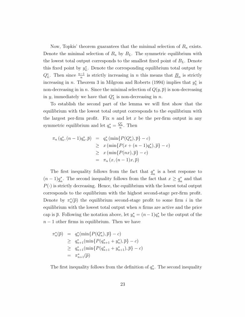
Now, Topkis’ theorem guarantees that the minimal selection of Bn exists.

Denote the minimal selection of Bn by BL. The symmetric equilibrium with

the lowest total output corresponds to the smallest fixed point of BL. Denote

this fixed point by y∗L. Denote the corresponding equilibrium total output by

Q∗L. Then since n−1n

is strictly increasing in n this means that Bn is strictly

increasing in n. Theorem 3 in Milgrom and Roberts (1994) implies that y∗L is

non-decreasing in in n. Since the minimal selection of Q(y, p) is non-decreasing

in y, immediately we have that Q∗L is non-decreasing in n.

To establish the second part of the lemma we will first show that the

equilibrium with the lowest total output corresponds to the equilibrium with

the largest per-firm profit. Fix n and let x be the per-firm output in any

symmetric equilibrium and let q∗n = Q∗nn

. Then

πn (q∗n, (n− 1)q∗n, p) = q∗n (min{P (Q∗n), p} − c)≥ x (min{P (x+ (n− 1)q∗n), p} − c)≥ x (min{P (nx), p} − c)= πn (x, (n− 1)x, p)

The first inequality follows from the fact that q∗n

is a best response to

(n − 1)q∗n. The second inequality follows from the fact that x ≥ q∗

nand that

P (·) is strictly decreasing. Hence, the equilibrium with the lowest total output

corresponds to the equilibrium with the highest second-stage per-firm profit.

Denote by π∗n(p) the equilibrium second-stage profit to some firm i in the

equilibrium with the lowest total output when n firms are active and the price

cap is p. Following the notation above, let y∗n = (n− 1)q∗n be the output of the

n− 1 other firms in equilibrium. Then we have

π∗n(p) = q∗n(min{P (Q∗n), p} − c)≥ q∗n+1(min{P (q∗n+1 + y∗n), p} − c)≥ q∗n+1(min{P (q∗n+1 + y∗n+1), p} − c)= π∗n+1(p)

The first inequality follows from the definition of q∗n. The second inequality

23

follows from the fact that y∗n is non-decreasing in n, as demonstrated above.

This establishes the claim.

Proof of Lemma 3.2

Proof. Fix n ∈ N. Let p1 > p2 and note that

π∗n(p1) = q∗n(p1)(min{P (Q∗n(p1)), p1} − c)≥ q∗n(p2)(min{P (q∗n(p2) + (n− 1)q∗n(p1)), p1} − c)≥ q∗n(p2)(min{P (q∗n(p2) + (n− 1)q∗n(p1)), p2} − c)≥ q∗n(p2)(min{P (q∗n(p2) + (n− 1)q∗n(p2)), p2} − c)= π∗n(p2)

The first inequality follows from the fact that q∗n(p1) is a best response

to (n − 1)q∗n(p1). The second inequality follows since p1 > p2. The third

inequality follows from the fact that for fixed n EST prove (in Theorem 1)

that minimal equilibrium output per firm is non-increasing in the price cap.

This means q∗n(p2) ≥ q∗n(p1). Since P (·) is decreasing, the inequality holds.

This establishes the lemma

Proof of Lemma 3.3

Proof. Let p1 > p2. Let ni be the equilibrium number of firms under pi,

i ∈ {1, 2}. We will establish the claim by contradiction. So, suppose n2 > n1.

By definition, ni must satisfy π∗ni(pi) ≥ K and π∗m(pi) < K for m > ni. Since

n2 > n1, we must have π∗n2(p1) < K. But by lemma (3.2) we must have

π∗n2(p1) ≥ π∗n2

(p2) ≥ K which is a contradiction.

Proof of Proposition 1

Part (i)

24

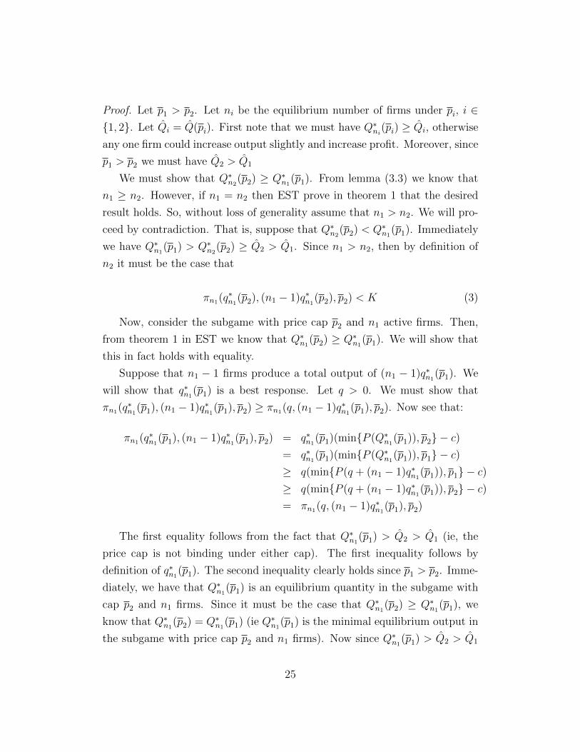
Proof. Let p1 > p2. Let ni be the equilibrium number of firms under pi, i ∈{1, 2}. Let Q̂i = Q̂(pi). First note that we must have Q∗ni

(pi) ≥ Q̂i, otherwise

any one firm could increase output slightly and increase profit. Moreover, since

p1 > p2 we must have Q̂2 > Q̂1

We must show that Q∗n2(p2) ≥ Q∗n1

(p1). From lemma (3.3) we know that

n1 ≥ n2. However, if n1 = n2 then EST prove in theorem 1 that the desired

result holds. So, without loss of generality assume that n1 > n2. We will pro-

ceed by contradiction. That is, suppose that Q∗n2(p2) < Q∗n1

(p1). Immediately

we have Q∗n1(p1) > Q∗n2

(p2) ≥ Q̂2 > Q̂1. Since n1 > n2, then by definition of

n2 it must be the case that

πn1(q∗n1

(p2), (n1 − 1)q∗n1(p2), p2) < K (3)

Now, consider the subgame with price cap p2 and n1 active firms. Then,

from theorem 1 in EST we know that Q∗n1(p2) ≥ Q∗n1

(p1). We will show that

this in fact holds with equality.

Suppose that n1 − 1 firms produce a total output of (n1 − 1)q∗n1(p1). We

will show that q∗n1(p1) is a best response. Let q > 0. We must show that

πn1(q∗n1

(p1), (n1 − 1)q∗n1(p1), p2) ≥ πn1(q, (n1 − 1)q∗n1

(p1), p2). Now see that:

πn1(q∗n1

(p1), (n1 − 1)q∗n1(p1), p2) = q∗n1

(p1)(min{P (Q∗n1(p1)), p2} − c)

= q∗n1(p1)(min{P (Q∗n1

(p1)), p1} − c)≥ q(min{P (q + (n1 − 1)q∗n1

(p1)), p1} − c)≥ q(min{P (q + (n1 − 1)q∗n1

(p1)), p2} − c)= πn1(q, (n1 − 1)q∗n1

(p1), p2)

The first equality follows from the fact that Q∗n1(p1) > Q̂2 > Q̂1 (ie, the

price cap is not binding under either cap). The first inequality follows by

definition of q∗n1(p1). The second inequality clearly holds since p1 > p2. Imme-

diately, we have that Q∗n1(p1) is an equilibrium quantity in the subgame with

cap p2 and n1 firms. Since it must be the case that Q∗n1(p2) ≥ Q∗n1

(p1), we

know that Q∗n1(p2) = Q∗n1

(p1) (ie Q∗n1(p1) is the minimal equilibrium output in

the subgame with price cap p2 and n1 firms). Now since Q∗n1(p1) > Q̂2 > Q̂1

25

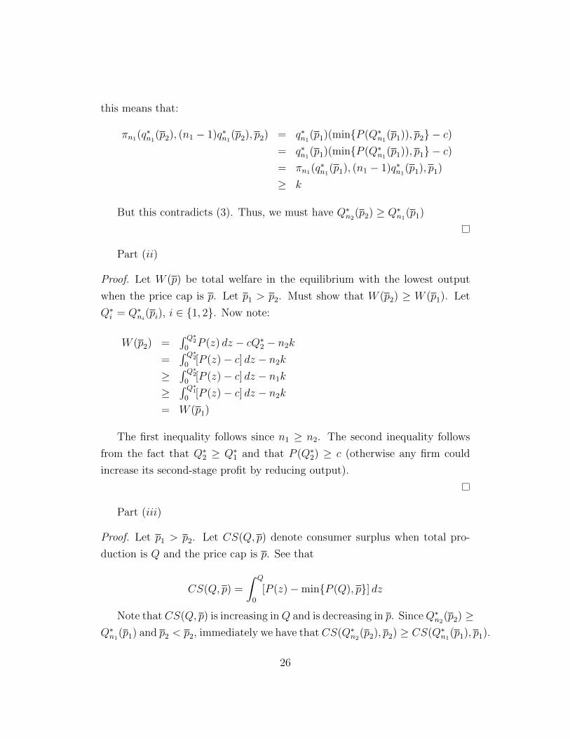
this means that:

πn1(q∗n1

(p2), (n1 − 1)q∗n1(p2), p2) = q∗n1

(p1)(min{P (Q∗n1(p1)), p2} − c)

= q∗n1(p1)(min{P (Q∗n1

(p1)), p1} − c)= πn1(q

∗n1

(p1), (n1 − 1)q∗n1(p1), p1)

≥ k

But this contradicts (3). Thus, we must have Q∗n2(p2) ≥ Q∗n1

(p1)

Part (ii)

Proof. Let W (p) be total welfare in the equilibrium with the lowest output

when the price cap is p. Let p1 > p2. Must show that W (p2) ≥ W (p1). Let

Q∗i = Q∗ni(pi), i ∈ {1, 2}. Now note:

W (p2) =∫ Q∗20P (z) dz − cQ∗2 − n2k

=∫ Q∗20

[P (z)− c] dz − n2k

≥∫ Q∗20

[P (z)− c] dz − n1k

≥∫ Q∗10

[P (z)− c] dz − n2k

= W (p1)

The first inequality follows since n1 ≥ n2. The second inequality follows

from the fact that Q∗2 ≥ Q∗1 and that P (Q∗2) ≥ c (otherwise any firm could

increase its second-stage profit by reducing output).

Part (iii)

Proof. Let p1 > p2. Let CS(Q, p) denote consumer surplus when total pro-

duction is Q and the price cap is p. See that

CS(Q, p) =

∫ Q

0

[P (z)−min{P (Q), p}] dz

Note that CS(Q, p) is increasing inQ and is decreasing in p. SinceQ∗n2(p2) ≥

Q∗n1(p1) and p2 < p2, immediately we have that CS(Q∗n2

(p2), p2) ≥ CS(Q∗n1(p1), p1).

26

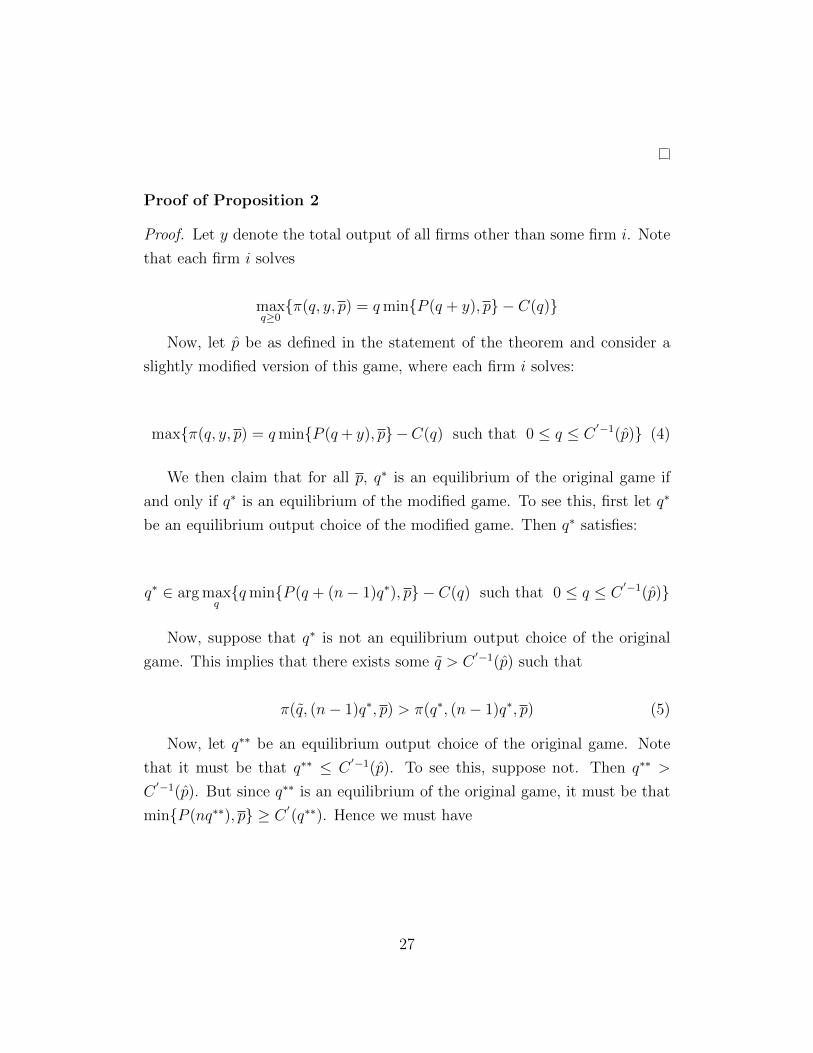
Proof of Proposition 2

Proof. Let y denote the total output of all firms other than some firm i. Note

that each firm i solves

maxq≥0{π(q, y, p) = qmin{P (q + y), p} − C(q)}

Now, let p̂ be as defined in the statement of the theorem and consider a

slightly modified version of this game, where each firm i solves:

max{π(q, y, p) = qmin{P (q+ y), p}−C(q) such that 0 ≤ q ≤ C′−1(p̂)} (4)

We then claim that for all p, q∗ is an equilibrium of the original game if

and only if q∗ is an equilibrium of the modified game. To see this, first let q∗

be an equilibrium output choice of the modified game. Then q∗ satisfies:

q∗ ∈ arg maxq{qmin{P (q + (n− 1)q∗), p} − C(q) such that 0 ≤ q ≤ C

′−1(p̂)}

Now, suppose that q∗ is not an equilibrium output choice of the original

game. This implies that there exists some q̃ > C′−1(p̂) such that

π(q̃, (n− 1)q∗, p) > π(q∗, (n− 1)q∗, p) (5)

Now, let q∗∗ be an equilibrium output choice of the original game. Note

that it must be that q∗∗ ≤ C′−1(p̂). To see this, suppose not. Then q∗∗ >

C′−1(p̂). But since q∗∗ is an equilibrium of the original game, it must be that

min{P (nq∗∗), p} ≥ C′(q∗∗). Hence we must have

27

P (nq∗∗) ≥ C′(q∗∗)

> C′(C′−1(p̂))

= p̂

= P (nC′−1(p̂))

But this immediately implies that q∗∗ < C′−1(p̂) which is a contradiction.

Thus, q∗∗ ≤ C′−1(p̂). Hence, q∗∗ is a feasible output choice of the modified

game. By the optimality of q∗ when the other firms choose (n − 1)q∗, this

means

π(q∗, (n− 1)q∗, p) ≥ π(q∗∗, (n− 1)q∗, p) (6)

Finally, by the optimality of q∗∗ when the other firms choose output (n−1)q∗∗ we must have

π(q∗∗, (n− 1)q∗∗, p) ≥ π(q̃, (n− 1)q∗∗, p) (7)

Inequalities (5) and (6) imply that

π(q̃, (n− 1)q∗, p) > π(q∗∗, (n− 1)q∗, p)

Combining this fact with (7) we see that:

π(q̃, (n−1)q∗, p)−π(q∗∗, (n−1)q∗, p) > 0 ≥ π(q̃, (n−1)q∗∗, p)−π(q∗∗, (n−1)q∗∗, p)

Equivalently,

π(q̃, (n−1)q∗, p)−π(q̃, (n−1)q∗∗, p) > 0 ≥ π(q∗∗, (n−1)q∗, p)−π(q∗∗, (n−1)q∗∗, p)

(8)

Now note that for any q and any p, π(q, y, p) is non-increasing in y. Then

the left-hand side of (8) implies that (n − 1)q∗ < (n − 1)q∗∗, while the right-

hand side of (8) implies that (n− 1)q∗ ≥ (n− 1)q∗∗ which is a contradiction.

28

Hence, it must be that q∗ is an equilibrium output choice of the original game.

Now, suppose that q∗ is an equilibrium of the original game. As shown

above, it must be that q∗ ≤ C′−1(p̂). The fact that q∗ is an equilibrium of the

modified game is then immediate. Thus, q∗ is an equilibrium output choice

of the original game if and only if q∗ is an equilibrium output choice of the

modified game.

We claim that for all p > p̂ the maximand in (4) satisfies the single-crossing

property in (q;−p) for each y. To establish the claim, fix y ≥ 0 and let

p′ > p > p̂ and let q < q′ ≤ C′−1(p̂). Assume that π(q′, y, p′) > π(q, y, p′). We

will show that this implies π(q′, y, p) > π(q, y, p). To do this, we will seperately

examine three cases.

(a) First, suppose that the price cap p binds for both quantities q and q′.

Then since p > p̂ immediately it must be that C′(q) < C

′(q′) ≤ p̂ < p.

Hence, π(z, y, p) = zp − C(z) is strictly increasing in z for all z ∈ [q, q′].

This immediately implies that π(q′, y, p) > π(q, y, p)

(b) Next, suppose that the price cap, p binds for q but not for q′. Since, the

lower cap does not bind for output q′, the higher cap must not have been

binding either. So,

π(q′, y, p) = π(q′, y, p′)

> π(q, y, p′)

≥ π(q, y, p)

(c) If the cap does not bind for either quantity, then the profits are the same

under p as they were under p′

Hence, for all p > p̂ and for all y, the maximand in (4) satisfies the single-

crossing property in (q;−p). Let q(y, p) denote the argmax of (4). Then

since the maximand in (4) satisfies the single-crossing property in (q;−p),the feasible correspondence is constant in p, and profit is continuous in own

output, then theorem 4 in Milgrom and Shannon implies that the minimal and

maximal selections of q(y, p) are non-increasing in p.

29

As done in the proof of lemma (3.1), it will be useful to think of a firm

choosing cumulative output, Q, of the modified game given the other firms

produce y. Let Q ≡ x+ y and let Q(y, p) be defined as follows

Q(y, p) = arg max{(Q−y) min{P (Q), p}−C(Q−y) s.t. y ≤ Q ≤ y+C′−1(p̂)}

(9)

Note that Q(y, p) solves (9) if and only if q(y, p) = Q(y, p) − y solves

(4). Now, using an identical argument as given in the proof of lemma 3.4,

the maximand in (9) has strict increasing differences in (Q, y) on the feasible

lattice. Finally, the feasible correspondence is ascending in y. Hence, every

selection of Q(y, p) is non-decreasing in y for fixed p.

Using the definition of q(y, p) given above, define the following correspon-

dence:

Bp(y) =n− 1

n(q(y, p) + y)

As argued in the proof of lemma 3.1, the maximal and minimal selections of

B exist (denote these BL and BH , respectively) and the minimal and maximal

equilibrium outputs (of the modified game) correspond to the smallest and

largest fixed points of BL and BH , respectively.

Now, since every selection of Q(y, p) = q(y, p) + y is non-decreasing in y,

it holds that every selection of B is non-decreasing in y. Moreover, as argued

above the smallest and largest selections of q(y, p) are non-increasing in p.

Hence, BL and BH are non-increasing in p.

Then, by theorem 3 in Milgrom and Shannon (1994), the smallest and

largest fixed points of B (denote these y∗L(p) and y∗H(p), respectively) are non-

increasing in p.

Since every selection of Q(y, p) is non-decreasing in y, and y∗L(p) and y∗H(p)

are non-increasing in p, it follows that the smallest and largest aggregate equi-

librium outputs, Q∗L(p) and Q∗H(p), are non-increasing in p. This means that

the smallest and largest equilibrium outputs of the modified game are non-

increasing in the price cap. But as shown previously, the equilibria of this

30

modified game are the same as the equilibria of the original game. Hence,

the smallest and largest equilibrium outputs of the original game must be

non-increasing in the price cap (for caps above p̂).

To establish part (ii), note that equilibrium welfare under some price cap

p is given by:

W ∗(p) =∫ Q∗(p)0

P (z) dz − nC(Q∗(p)n

)=

∫ Q∗(p)0

[P (z)− C ′

(zn

)]dz

Where q∗(p) denotes either the smallest or largest equilibrium per-firm

output and Q∗(p) = nq∗(p). Since it must be that P (Q∗(p)) ≥ C′(q∗) it

must be that for all z ∈ [0, Q∗(p)] we have P (Q∗(p)) > C′(q∗). Then for all

p > p̂ it follows that Q∗(p) is non-increasing in p. Thus, equilibrium welfare is

non-increasing in p for all p > p̂. This establishes part (ii).

To establish part (iii), we will first show that output and welfare are non-

decreasing in the cap for all p < p̂. So, fix p < p̂, let q∗ denote an equilibrium

output choice under the cap and let Q∗ = nq∗. First, suppose that P (Q∗) ≤p. Since, p < p̂ this means p < P (nC

′−1(p)). So, we must have P (Q∗) <

P (nC′−1(p)). But this means q∗ > C

′−1(p) which implies C ′(q∗) > p > P (Q∗)

which contradicts the optimality of q∗. Thus, we must have P (Q∗) < p. So,

per-firm equilibrium profit must be given by π(q∗, (n− 1)q∗, p) = q∗p−C(q∗).

Clearly, in this case any output choice other than q∗ = C′−1(p) is sub optimal

assuming profit at this level of output is positive (If profit is not positive at

this level of output then each firm produces zero.)

Now, let p = p̂. By an argument similar to that made above, and using the

fact that profit is positive if each firm produces q = C′−1(p̂), it may be verified

that equilibrium output is strictly positive and satisfiesq∗ = C′−1(p) = C

′−1(p̂).

Hence, P (Q∗) = p = p̂

Since, C′−1 is strictly increasing, it must be that equilibrium output strictly

decreases as we lower the cap below p̂. An argument analogous to that given

for part (ii) may establish that equilibrium welfare strictly decreases as we

lower the cap below p̂.

31

Finally, since it must be that p̂ < p∞, and by the argument given above it

must be that P (Q∗) = p̂. This means Q∗ > Q∞. So, when the cap is equal to

p̂ equilibrium output must be strictly greater than equilibrium output in the

absence of a cap. It holds that welfare must be strictly higher under the cap

than in the absence of the cap.

Proof of Lemma 3.4

Proof. From the proof of lemma (3.1) in the constant marginal cost case, it

can be seen that the sufficient condition for the conclusion to hold9 is for

π̃(Q, y, p) ≡ (Q − y) min{P (Q), p} − C(Q − y) to satisfy the single crossing

property in (Q; y) on the lattice

Φ ≡ {(Q, y)| 0 ≤ y ≤ (n− 1)M, y ≤ Q ≤ y +M}

Here, we will demonstrate that π̃ has strictly increasing differences in (Q, y)

which then implies that the single-crossing property is satisfied. The remainder

of the argument follows from the previous proof.

Now let Q′ > Q, y′ > y where Q′ > y′ and Q > y. Then π̃ has strict ID in

(Q, y) on Φ if and only if

π̃(Q′, y′)− π̃(Q′, y) > π̃(Q, y′)− π̃(Q, y)

Plugging in, and collecting like terms we see that the above expression is

equivalent to

(y′−y) [min{P (Q), p} −min{P (Q′), p}] > C(Q′−y′)−C(Q′−y)+C(Q−y)−C(Q−y′)(10)

Note that Q′ > Q, y′ > y and the fact that P (·) is strictly decreasing,

means the left-hand side of (10) is weakly positive. Now see that the right-

hand side of (10) is strictly negative if and only if

9See Amir and Lambson (2000)

32

C(Q′ − y′)− C(Q′ − y) < C(Q− y′)− C(Q− y) (11)

Define the function H(Q, y) ≡ C(Q− y). Note that (11) is satisfied if and

only if H has strict decreasing differences (DD) on Φ. But note that since H

is differentiable on Φ, if the cross partial derivative of H with respect to Q and

y is strictly negative, then H has strict DD. Then, see that the cross partial

derivative of H with respect to Q and y is given by −C ′′(Q− y) < 0. Hence,

the right-hand side of (10) is strictly less than zero.

This establishes that π̃ has strict ID on Φ. The remainder of the proof is

identical to the proof with constant marginal cost.

Proof of Lemma 3.5

Proof. First, note that since p ≥ ATCm it is profitable for at least one firm to

enter. To establish the claim, lemma (3.4) implies that it suffices to show that

in the subgame with n∞ firms and a price cap p, equilibrium profit is strictly

less than the cost of entry.

Fix p ∈ [ATCm, p∞). Let Q∗ be the equilibrium total output in the sub-

game with n∞ firms with price cap p. Let q∗ = Q∗

n∞. Finally, let π∗ denote

equilibrium second-stage profit with n∞ firms and a price cap.

First, suppose q∗ > q∞. Then we have:

K = q∞P (Q∞)− C(q∞)

≥ q∗P (q∗ + (n∞ − 1)q∞)− C(q∗)

> q∗P (Q∗)− C(q∗)

≥ q∗min{P (Q∗), p} − C(q∗)

= π∗

The first inequality follows by definition of q∞, while the strict inequality

follows since q∗ > q∞. Now suppose that q∗ ≤ q∞. See that:

33

K = q∞P (Q∞)− C(q∞)

≥ q∗P (Q∞)− C(q∗)

> q∗p− C(q∗)

≥ q∗min{P (Q∗), p} − C(q∗)

= π∗

To see why the first inequality holds, note that Q∞ must satisfy P (Q∞) >

C ′(q∞). But this means P (Q∞) > C ′(x) for all x ∈ [0, q∞]. Hence, the

function xP (Q∞) − C(x) is strictly increasing in x for x ∈ [0, q∞]. Since

q∗ ≤ q∞, the inequality holds. Finally, note that the strict inequality follows

since p < P (Q∞).

Hence, we must have π∗ < K.

Proof of Proposition 3

Proof. First note that since the entry constraint is binding, by Lemma (3.5)

any price cap, p ∈ [ATCm, p∞), results in the entrance of at least one firm and

at most n∞ − 1 firms. First, consider the subgame with n∞ − 1 firms under

a price cap p ∈ [ATCm, p∞). We will then show that maximal equilibrium

profit in this subgame is at least as large as the cost of entry.

Let π(Q, y, p) = (Q − y) min{P (Q), p} − C(Q − y) be profit for a firm if

total output is Q, rivals’ output is y, and the price cap is p ∈ [ATCm, p∞).

Initially we suppose that y = (n − 2)C ′−1(p); that is, each rival firm sets its

output such that marginal cost is equal to the price cap. Note that π(Q, y, p)

is continuous in Q. Also

πQ(Q, y, p) =

{p− C ′(Q− y), Q < P−1(p)

P (Q)− (Q− y)P ′(Q)− C ′(Q− y), Q > P−1(p)

For Q > P−1(p) we have the following inequalities:

πQ(Q, y, p) < p− C ′(Q− y) < 0, (12)

34

where the first inequality follows because the inverse demand function is strictly

decreasing in Q. The second inequality is due to the following argument. First,

the assumption that C ′( Q∞

n∞−1) > p∞ implies that, Q∞ > (n∞ − 1)C ′−1(p∞) ≥(n∞ − 1)C ′−1(p) = y + C ′−1(p). Second, Q > P−1(p) implies Q > Q∞ so,

Q − y > C ′−1(p). Third, this implies that p − C ′(Q − y) < 0, which is the

second inequality in equation (12) above.

Since the payoff function is strictly decreasing in Q for Q > P−1(p), it must

be that the best response Q to y is in the interval, [y, P−1(p)]. Strict convexity

of the cost function implies that the payoff function is strictly concave in Q in

this interval. The unique best response to y satisfies, p = C ′(Q−y); that is, it

is optimal for a firm to set its output such that marginal cost is equal to the

price cap when each of its rivals follows the same policy. The optimal choice

of Q is in the interior of [y, P−1(p)] since (by assumption) C ′( Q∞

n∞−1) > p∞.

q∗ = C ′−1(p) is equilibrium output per firm in the subgame with n∞−1 firms.

A proof-by-contradiction can be used to show that this is the unique subgame

equilibrium. Equilibrium profit is given by π∗(p) = q∗p− C(q∗)

To demonstrate (i), we show that in the subgame with n∞− 1 firms for all

p ∈ [ATCm, p∞) we have π∗(p) ≥ K. Let qm solve minxATC(x). Then see

that:

π∗(p) = q∗p− C(q∗)

≥ qmp− C(qm)

≥ qmATCm − C(qm) = K

The first inequality follows by the optimality of q∗ and the second follows

since p ≥ ATCm. Hence, the equilibrium number of firms is n∞ − 1. Then

since C ′′ > 0, we have that q∗ is increasing in p. Moreover, since p < p∞, we

must have P((n∞ − 1)C

′−1(p))> P

((n∞ − 1)C

′−1(p∞))> p∞. So, (n∞ −

1)C′−1(p) < Q∞. This establishes (i)− (iii).

Finally, note that for any relevant cap, equilibrium welfare is given by:

35

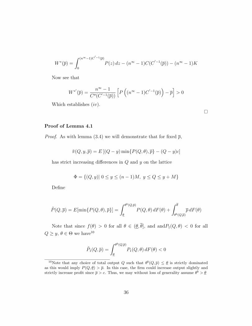
W ∗(p) =

∫ (n∞−1)C′−1(p)

0

P (z) dz − (n∞ − 1)C(C′−1(p))− (n∞ − 1)K

Now see that

W ∗′(p) =n∞ − 1

C ′′(C ′−1(p))

[P(

(n∞ − 1)C′−1(p)

)− p]> 0

Which establishes (iv).

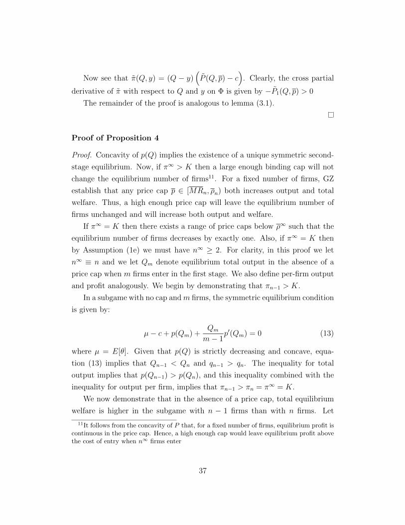
Proof of Lemma 4.1

Proof. As with lemma (3.4) we will demonstrate that for fixed p,

π̃(Q, y, p) = E [(Q− y) min{P (Q, θ), p} − (Q− y)c]

has strict increasing differences in Q and y on the lattice

Φ = {(Q, y)| 0 ≤ y ≤ (n− 1)M, y ≤ Q ≤ y +M}

Define

P̃ (Q, p) = E[min{P (Q, θ), p}] =

∫ θb(Q,p)

θ

P (Q, θ) dF (θ) +

∫ θ

θb(Q,p)

p dF (θ)

Note that since f(θ) > 0 for all θ ∈ (θ, θ], and andP1(Q, θ) < 0 for all

Q ≥ y, θ ∈ Θ we have10

P̃1(Q, p) =

∫ θb(Q,p)

θ

P1(Q, θ) dF (θ) < 0

10Note that any choice of total output Q such that θb(Q, p) ≤ θ is strictly dominatedas this would imply P (Q, θ) > p. In this case, the firm could increase output slightly andstrictly increase profit since p > c. Thus, we may without loss of generality assume θb > θ

36

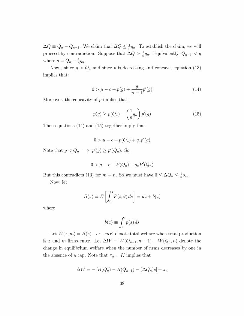
Now see that π̃(Q, y) = (Q − y)(P̃ (Q, p)− c

). Clearly, the cross partial

derivative of π̃ with respect to Q and y on Φ is given by −P̃1(Q, p) > 0

The remainder of the proof is analogous to lemma (3.1).

Proof of Proposition 4

Proof. Concavity of p(Q) implies the existence of a unique symmetric second-

stage equilibrium. Now, if π∞ > K then a large enough binding cap will not

change the equilibrium number of firms11. For a fixed number of firms, GZ

establish that any price cap p ∈ [MRn, ρn) both increases output and total

welfare. Thus, a high enough price cap will leave the equilibrium number of

firms unchanged and will increase both output and welfare.

If π∞ = K then there exists a range of price caps below ρ∞ such that the

equilibrium number of firms decreases by exactly one. Also, if π∞ = K then

by Assumption (1e) we must have n∞ ≥ 2. For clarity, in this proof we let

n∞ ≡ n and we let Qm denote equilibrium total output in the absence of a

price cap when m firms enter in the first stage. We also define per-firm output

and profit analogously. We begin by demonstrating that πn−1 > K.

In a subgame with no cap andm firms, the symmetric equilibrium condition

is given by:

µ− c+ p(Qm) +Qm

m− 1p′(Qm) = 0 (13)

where µ = E[θ]. Given that p(Q) is strictly decreasing and concave, equa-

tion (13) implies that Qn−1 < Qn and qn−1 > qn. The inequality for total

output implies that p(Qn−1) > p(Qn), and this inequality combined with the

inequality for output per firm, implies that πn−1 > πn = π∞ = K.

We now demonstrate that in the absence of a price cap, total equilibrium

welfare is higher in the subgame with n − 1 firms than with n firms. Let

11It follows from the concavity of P that, for a fixed number of firms, equilibrium profit iscontinuous in the price cap. Hence, a high enough cap would leave equilibrium profit abovethe cost of entry when n∞ firms enter

37

∆Q ≡ Qn −Qn−1. We claim that ∆Q ≤ 1nqn. To establish the claim, we will

proceed by contradiction. Suppose that ∆Q > 1nqn. Equivalently, Qn−1 < g

where g ≡ Qn − 1nqn.

Now , since g > Qn and since p is decreasing and concave, equation (13)

implies that:

0 > µ− c+ p(g) +g

n− 1p′(g) (14)

Moreover, the concavity of p implies that:

p(g) ≥ p(Qn)−(

1

nqn

)p′(g) (15)

Then equations (14) and (15) together imply that

0 > µ− c+ p(Qn) + qnp′(g)

Note that g < Qn =⇒ p′(g) ≥ p′(Qn). So,

0 > µ− c+ P (Qn) + qnP′(Qn)

But this contradicts (13) for m = n. So we must have 0 ≤ ∆Qn ≤ 1nqn.

Now, let

B(z) ≡ E

[∫ z

0

P (s, θ) ds

]= µz + b(z)

where

b(z) ≡∫ z

0

p(s) ds

Let W (z,m) = B(z)−cz−mK denote total welfare when total production

is z and m firms enter. Let ∆W ≡ W (Qn−1, n − 1) −W (Qn, n) denote the

change in equilibrium welfare when the number of firms decreases by one in

the absence of a cap. Note that πn = K implies that

∆W = − [B(Qn)−B(Qn−1)− (∆Qn)c] + πn

38

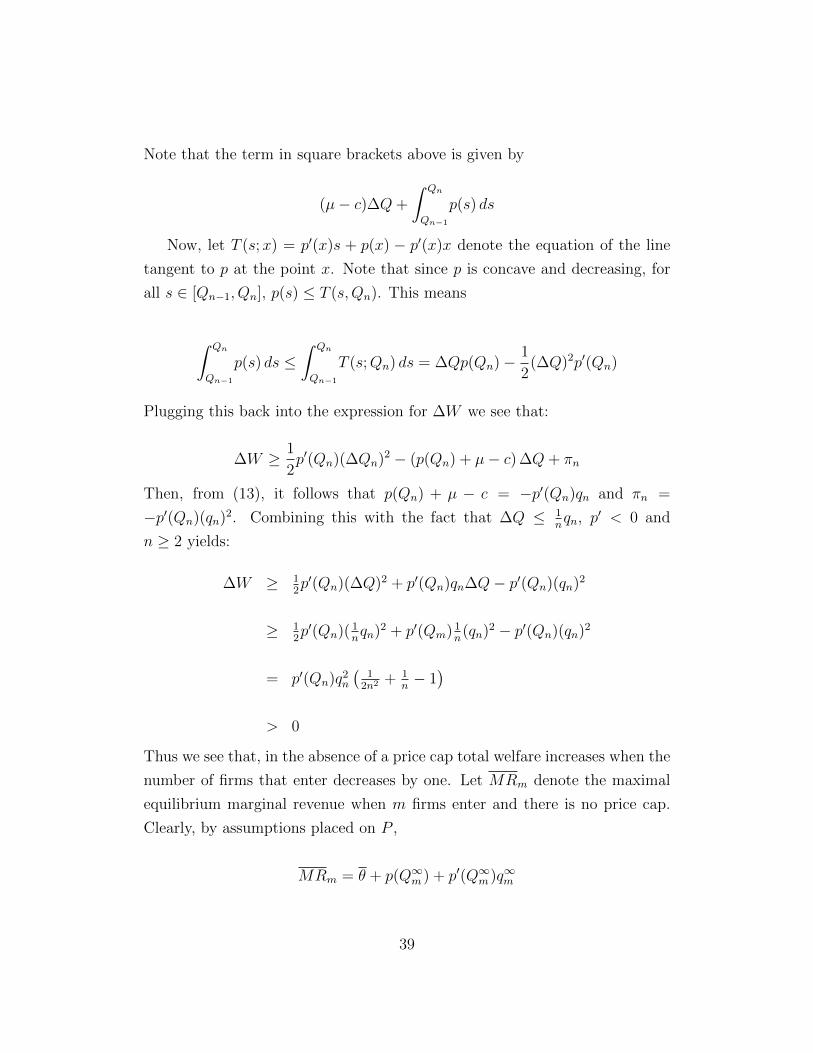
Note that the term in square brackets above is given by

(µ− c)∆Q+

∫ Qn

Qn−1

p(s) ds

Now, let T (s;x) = p′(x)s + p(x) − p′(x)x denote the equation of the line

tangent to p at the point x. Note that since p is concave and decreasing, for

all s ∈ [Qn−1, Qn], p(s) ≤ T (s,Qn). This means

∫ Qn

Qn−1

p(s) ds ≤∫ Qn

Qn−1

T (s;Qn) ds = ∆Qp(Qn)− 1

2(∆Q)2p′(Qn)

Plugging this back into the expression for ∆W we see that:

∆W ≥ 1

2p′(Qn)(∆Qn)2 − (p(Qn) + µ− c) ∆Q+ πn

Then, from (13), it follows that p(Qn) + µ − c = −p′(Qn)qn and πn =

−p′(Qn)(qn)2. Combining this with the fact that ∆Q ≤ 1nqn, p′ < 0 and

n ≥ 2 yields:

∆W ≥ 12p′(Qn)(∆Q)2 + p′(Qn)qn∆Q− p′(Qn)(qn)2

≥ 12p′(Qn)( 1

nqn)2 + p′(Qm) 1

n(qn)2 − p′(Qn)(qn)2

= p′(Qn)q2n(

12n2 + 1

n− 1)

> 0

Thus we see that, in the absence of a price cap total welfare increases when the

number of firms that enter decreases by one. Let MRm denote the maximal

equilibrium marginal revenue when m firms enter and there is no price cap.

Clearly, by assumptions placed on P ,

MRm = θ + p(Q∞m ) + p′(Q∞m )q∞m

39

By the first order equilibrium conditions, it follows that p(Q∞m ) + p′(Q∞m )q∞m =

c− µ. Hence, independent of m it is clear that

MRm = θ + c− µ

and since p′ < 0:

MRm < θ + p(Q∞m ) = ρm

Since MRm is independent of m, we drop this subscript and write MR.

Let ρm = P (Q∞m , θ). Now, since π∞ = K and πn−1 > K, there exists a range

of price caps strictly less than ρn such that the equilibrium number of firms

will decrease by exactly one12. Let p̂1 denote the smallest of these price caps.

Let p̂ ≡ max{p̂1,MR}. Then since MR < ρn and p̂1 < ρn we have p̂ < ρn.

Also see that under any price cap p ∈ [p̂, ρn) the equilibrium number of firms

is n− 1. Finally note that by lemma (4.1) it is clear that ρn ≤ ρn−1.

Choose p ∈ [p̂, ρn). Then since p ∈ [MR, ρn−1) by GZ Theorem 1, it

follows that equilibrium welfare under the price cap is strictly greater than

equilibrium welfare in the subgame with n− 1 firms and no cap. Since welfare

in the absence of a cap when n − 1 firms enter is strictly higher than welfare

when n firms enter, the result follows.

Proof of Lemma 4.2

Proof. By the definition of θ̃(Xm) and θ̃(Xm) note that the first-order condition

given in (??) may be re-written as:

∫ θ

θ̃(Xm)

[θ − θ̃(Xm)

]dF (θ) =

∫ θ

θ̃(Xn)

[θ − θ̃(Xn)

]dF (θ) = c

Let G(s) =∫ θs[θ − s ]dF (θ) and note that G′(s) =

∫ θs−1 dF (θ). Note

that G′(s) < 0 for all s < θ. Then, the first-order conditions imply that

12Once again, this follows since concavity of P implies the continuity of equilibrium profitin the price cap

40

G(θ̃(Xm)) = G(θ̃(Xn)). Since θ̃(Xm) < θ and θ̃(Xn) < θ it must be that

θ̃(Xm) = θ̃(Xn)

Proof of Lemma 4.3

Proof. First, by lemma (4.2) it follows that θ̃(Xn) = θ̃(Xn−1) = θ̃. First, fix

θ < θ̃. In this case we have Qn(θ) = Q̃n(θ) and Qn−1(θ) = Q̃n−1(θ). Both

output choices must satisfy their respective first-order conditions:

θ + p(Q̃n(θ)) + q̃n(θ)p′(Q̃n(θ)) = 0

and

θ + p(Q̃n−1(θ)) + q̃n−1(θ)p′(Q̃n−1(θ)) = 0

From the first-order conditions, the concavity of p together with the fact

that p′ < 0 implies that Q̃n(θ) > Q̃n−1(θ) and q̃n(θ) < Q̃n−1(θ)

Now, since θ̃(Xn) = θ̃(Xn−1) = θ̃ it follows from the definitions of θ̃(Xn)

and θ̃(Xn−1) that

θ̃ + p(Xn) + xnp′(Xn) = 0

and

θ̃ + p(Xn−1) + xn−1p′(Xn−1) = 0

Once again, these equations together with our assumptions on p ensure

that Xn > Xn−1 and xn < xn−1

This establishes (i) and (ii)

Now see that

πn−1 =

∫ θ̃(Xn−1)

θ

q̃n−1(θ)[θ+p(Q̃n−1(θ))] dF (θ)+xn−1

(∫ θ

θ̃(Xn−1)

[θ + p(Xn−1) ]dF (θ)− c

)

41

Note that the first-order condition given in (??) implies that(∫ θ

θ̃(Xn−1)

[θ + p(Xn−1) ]dF (θ)− c

)> 0

Then by parts (i) and (ii) above, the result is immediate.

Proof of Proposition 5

Proof. As in the proof of Proposition 4, we demonstrate our result by showing

that welfare in the subgame with n firms and no price cap is strictly lower

than welfare in the subgame with n − 1 firms and no cap. For each θ ∈ Θ

let ∆Q(θ) ≡ Qn(θ) − Qn−1(θ). We will first demonstrate that for each θ,

∆Q(θ) ≤ 1nqn(θ).

Using the fact that θ̃(Xn) = θ̃(Xn−1) we first examine the case when θ < θ̃.

In this case, we use the first order conditions and the proof is identical to the

proof in the previous section. For the case when θ > θ̃ we again use the

definition of θ̃ and follow a similar argument as in the previous section.

Thus, for each θ ∆Q(θ) ≤ 1nqn(θ)

Now, let Wm denote equilibrium expected welfare in the subgame with m

firms. Let ∆W ≡ Wn−1 −Wn. Note that

Wn = E

[∫ Qn(θ)

0

[θ + p(s) ]ds

]− cXn − nπn

Which may be written:

Wn =

∫ θ̃

θ

[∫ Q̃n(θ)

0

[θ + p(s) ]ds

]dF (θ)+

∫ θ

θ̃

[∫ Xn

0

[θ + p(s)] ds

]dF (θ)−cXn−nπn

Let ∆W = Wn−1 −Wn and note that

42

∆W = −∫ θ̃

θ

[∫ Q̃n(θ)

Q̃n−1(θ)

[θ + p(s) ]ds

]dF (θ)−

∫ θ

θ̃

[∫ Xn

Xn−1

[θ + p(s)] ds

]dF (θ)+(∆X)c+πn

Now, following a similar argument as in the previous section, using the

concavity of p, we may show that for each θ ∈ [θ, θ̃]

∫ Q̃n(θ)

Q̃n−1(θ)

[θ + p(s) ]ds ≤ ∆Q̃(θ)(θ + p(Q̃n(θ)))− 1

2(∆Q̃(θ))2p′(Q̃n(θ)) ≡ A(θ)

Moreover, for each θ ∈ [θ̃, θ]∫ Xn

Xn−1

[θ + p(s) ]ds ≤ ∆X(θ + p(Xn))− 1

2(∆X)2p′(Xn) ≡ B(θ)

Now, using the first-order conditions we may write:

πn =

(−∫ θ̃

θ

(q̃n(θ))2p′(Q̃n(θ)) dF (θ)

)+

(−∫ θ

θ̃

(xn)2p′(Xn) dF (θ)

)≡ πAn +πBn

Hence, it follows that

∆W ≥ −∫ θ̃

θ

A(θ) dF (θ)−∫ θ

θ̃

B(θ) dF (θ) + (∆X)c+ πAn + πBn

Now, note that

−∫ θ̃

θ

A(θ) dF (θ)+πAn =

∫ θ̃

θ

[−∆Q̃(θ)(θ + p(Q̃n(θ))) +

1

2(∆Q̃(θ))2p′(Q̃n(θ))− (q̃n(θ))2p′(Q̃n(θ))

]dF (θ)

Using the first-order conditions once again, we know that for each θ ∈ [θ, θ̃]

it holds that θ + Q̃n = −q̃n(θ)p′(Q̃n). This, combined with the fact that

43

∆Q̃(θ) ≤ 1nq̃n(θ) allow us to write

−∫ θ̃

θ

A(θ) dF (θ) + πAn ≥∫ θ̃

θ

(q̃n(θ)p′(Q̃n(θ))

(1

n+

1

2n2− 1

)dF (θ) > 0

Now also see that

−∫ θθ̃B(θ) dF (θ) + (∆X)c+ πBn

= −∆X[∫ θ

θ̃(θ + p(Xn)) dF (θ)− c

]+∫ θθ̃

[12(∆X)2p′(Xn)− (xn)2p′(Xn)

]dF (θ)

From the first-order condition, it follows that

∫ θ

θ̃

(θ + p(Xn)) dF (θ)− c =

∫ θ

θ̃

−xnp′(Xn) dF (θ)

This, combined with the fact that ∆X ≤ 1nxn allows us to write:

−∫ θ

θ̃

B(θ) dF (θ) + (∆X)c+ πBn ≥ (xn)2p′(Xn)

∫ θ

θ̃

(1

n+

1

2n2− 1

)dF (θ) > 0

It follows immediately that ∆W > 0. The remainder of the proof works

identically to the previous section. The result follows.

References

[1] Rabah Amir and Val Lambson. On the effects of entry in cournot markets.

Review of Economic Studies, 67, 2000.

[2] Severin Borenstein, James Bushnell, and Frank Wolak. Measuring market

inefficiencies in california’s restructured wholesale electricity market. The

American Economic Review, 92(5), 2002.

44

[3] Rex Cottle and Myles Wallace. Economic effects of non-binding price

constraints. The Journal of Industrial Economics, 31(4):469–474, 1983.

[4] Robert Earle, Karl Schmedders, and Tymon Tatur. On price caps under

uncertainty. Review of Economic Studies, 74:93–111, 2007.

[5] Veronika Grimm and Gregor Zottl. Capacity choice under uncertainty:

The impact of market structure. University of Cologne Working Paper

Series in Economics, (23), 2006.

[6] Veronika Grimm and Gregor Zottl. Price regulation under demand un-

certainty. The B.E. Journal of Theoretical Economics, 10(1), 2010.

[7] N. Gregory Mankiw and Michael Whinston. Free entry and social ineffi-

ciency. The Rand Journal of Economics, 17(1):48–58, 1986.

[8] Paul Milgrom and John Roberts. Comparing equilibria. The American

Economic Review, 84(3), 1994.

[9] Paul Milgrom and Chris Shannon. Monotone comparative statics. Econo-

metrica, 62(1), 1994.

[10] Gregor Zottl. On optimal scarcity prices. International Journal of Indus-

trial Organization, 29(5), 2011.

45