Pressurized Water Reactor Simulated by TRACE

NUC E 470: Final Project report

Team Members: Nicholas Manuk and Troy Todd

Report Submitted: December 14, 2015

Abstract:

The following report indicates the methods we chose in creating a four loop PWR. The final product we were to create is a steady reactor that can return to steady state after a transient is implemented. The model we created would reach a theoretical steady state, by this we mean it would show steady state in our chosen plots but not in our output text file. We push through this difficult in the attempt to make a transient work that would increase our power %5. This did not work and we have thus omitted most graphs and tables dealing with this.

1

Table of Contents:

Abstract....................................................................................................................................... 1

Table of Contents........................................................................................................................ 2

List of Figures...............................................................................................................................3

List of Tables................................................................................................................................4 Introduction.................................................................................................................................5

Model Development....................................................................................................................6

Steam Generator......................................................................................................................6

Reactor Vessel/Cores and Pressurizer......................................................................................10

Pump.........................................................................................................................................16

Turbine..................................................................................................................................... 17

Results of Systems.......................................................................................................................19

Steam Generator......................................................................................................................19

Reactor Vessel/Cores and Pressurizer......................................................................................23

Pump.........................................................................................................................................26

Turbine..................................................................................................................................... 29

Plant at Steady State................................................................................................................... 30

Plant Transient............................................................................................................................ 38

Conclusions..................................................................................................................................39

Appendix..................................................................................................................................... 40

2

Figures:

Figure 1 – Model of Steam Generator implemented in TRACE....................................................7 Figure 2 – Representation of the PWR Reactor Vessel and all of its inner components [Source: Nuc E 470 Course Textbook]........................................................................................................11

Figure 3- Representation of the cross section of the reactor vessel. [Source: Nuc E Course Textbook].................................................................................................................................... 12

Figure 4– Inputs to Reactor Vessel Height...................................................................................12

Figure 5- Input Data on the Reactor Radial Rings........................................................................12

Figure 6 – The TRACE model of the completed Reactor Vessel and Pressurizer..........................15

Figure 7 – Model of Pump Test system in TRACE........................................................................17

Figure 8 – Control Block diagram for the Turbine Work..............................................................19

Figure 9 – Graph of Hot Leg and Cold Leg temperature..............................................................20

Figure 10 – Graph of mass flow rate in both Hot Leg and Cold Leg.............................................21

Figure 11 – Graph of Mass Flow Rate into and out of Steam Generator.....................................22

Figure 12 – Graph of Liquid Levels in Downcomer and Boiler.....................................................23

Figure 13 – Exit Mass Flow Rate for Hot Leg – Reactor Vessel....................................................24

Figure 14–Cold Leg Exit Temperature – Reactor Vessel..............................................................24

Figure 15 –Reactor Power – Reactor Vessel................................................................................25

Figure 2 – Hot Leg Exit Temperature – Reactor Vessel................................................................26

Figure 3 – Pressurizer Pressure Difference – Reactor Vessel.......................................................26

Figure 18- Pressurizer Water Level - Reactor Vessel...................................................................27

Figure 19- Mass Flow Rate from Hot Leg through Coolant Pump and into Cold Leg...................28

Figure 20- Pressure Levels from RCP into Cold Leg......................................................................29

Figure 21 – Turbine Power.......................................................................................................... 30

Figure 22 – Steady State Final Reactor Model.............................................................................31

Figure 4- Hot Leg Exit Mass Flow Rate - Steady State..................................................................32

3

Figure 24- Hot Leg Exit Temperature - Steady State....................................................................33

Figure 25- Hot Leg Exit Pressure - Steady State...........................................................................34

Figure 5 - Pump Pressures - Steady State....................................................................................35

Figure 6 - Steam Mass Flow out of SGs - Steady State.................................................................36

Figure 78 - Steam Temperature - Steady State............................................................................37

Figure 89- Water Levels in Boiler - Steady State..........................................................................38

Figure 30 - Cold Leg Exit Temp. - Steady State.............................................................................39

Tables:

Table 1 – List of Values implemented in Steam Generator seen in Figure 1................................12

Table 2 –Vessel and Core data.....................................................................................................14

Table 3 – Pressurizer, Pump, Surge Line, and Cold, Hot, and Crossover Leg data.......................16

Table 4 – Table of Data implemented into coolant pump test section........................................17

4

Introduction:

The nuclear power plant is one of the most incredible marvels of modern science that

there exists today. Nuclear power affects lives around the United States and all around the

world. Serving as one of the main power sources for homes and businesses, nuclear energy is

something to marvel. That being said, the control of a nuclear power plant is where all of this

magic begins. The proper control of a nuclear power plant, specifically a Pressurized Water

Reactor (PWR), includes not allowing coolant to boil, creating a proper mass flow over large

stretches of piping, and maintaining single or two phase flow as necessary. It is beneficial from

the standpoint of safety, economics, and efficiency standpoint that a nuclear reactor operates

well on all cylinders. This includes the steam generator, turbine, reactor vessel, and coolant

pump to name a few. The PWR utilizes highly pressurized and very heated water as a means of

heating up cooler water, converting it into steam, and having that steam spin a turbine to

produce massive amounts of electricity, while the hot water maintains its position in a loop

through the entire reactor.

In this experiment the program known as the Symbolic Nuclear Analysis Package (SNAP)

was used to model these steps, and investigate the differences in pressure, temperature, and

mass flow through several portions of the nuclear reactor facility, and most importantly,

evaluate its safety vs. expected results. The goal is to build individual reactor pieces (Steam

Generator, Reactor Vessel, Coolant pumps) and evaluate them individually to earn a better

appreciation and understanding of how they work, and ultimately put them all together to see

how one’s input affects another’s output and vice versa. This PWR will be modeled and the

results will be analyzed through the APT Plot application. An analysis on these plots will be

conducted, and a transient will be enacted during a simulation to further investigate how the

reactor behaves under new conditions. The experiment will conclude with a discussion of what

was learned and suggestions for future work.

5

Model Development:

Model Development of Steam Generator:

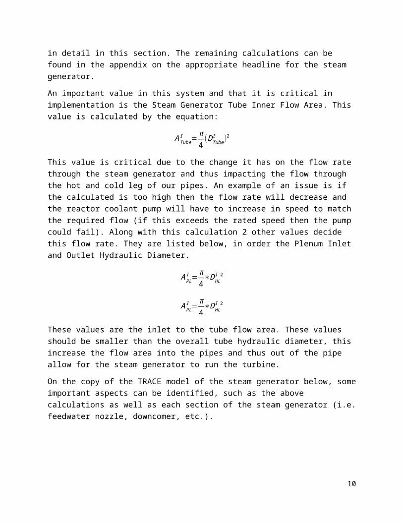
The steam generator we modeled is based off a given model from the stgenSS3.inp model presented throughout this course. The model we used is a simpler representation of a real steam generator. Steam generators that are implemented in power plants have many more items of interest that need to be considered such as heat transfer. This model needed several adjustments to the geometry to match what we planned on creating in our model. The table below lists the information used to create the steam generator. Also present is a copy of a single steam generator created in TRACE, only one is listed due to the other 3 being exact replicas of this model. To create the steam generator we would implement many calculations were needed to get exact values of our geometry. As seen in the table below the given values were useful in finding our values. Due to the number of calculations we needed to do only the most significant ones will be discussed in detail in this section. The remaining calculations can be found in the appendix on the appropriate headline for the steam generator.

An important value in this system and that it is critical in implementation is the Steam Generator Tube Inner Flow Area. This value is calculated by the equation:

ATubeI =π

4(DTube

I )2

This value is critical due to the change it has on the flow rate through the steam generator and thus impacting the flow through the hot and cold leg of our pipes. An example of an issue is if the calculated is too high then the flow rate will decrease and the reactor coolant pump will have to increase in speed to match the required flow (if this exceeds the rated speed then the pump could fail). Along with this calculation 2 other values decide this flow rate. They are listed below, in order the Plenum Inlet and Outlet Hydraulic Diameter.

APLI = π

4∗DHL

I 2

APLI = π

4∗DHL

I 2

These values are the inlet to the tube flow area. These values should be smaller than the overall tube hydraulic diameter, this increase the flow area into the pipes and thus out of the pipe allow for the steam generator to run the turbine.

On the copy of the TRACE model of the steam generator below, some important aspects can be identified, such as the above calculations as well as each section of the steam generator (i.e. feedwater nozzle, downcomer, etc.).

6

Figure 9 – Model of Steam Generator implemented in TRACE

1. Steam Generator Tube Bundle2. Steam Generator3. Transition Cone4. Feedwater Nozzle5. Steam Generator Downcomer6. Steam Generator Exit/Turbine Input7. Feedwater Input

Primary Side Given As-Built UnitsTube Outer Diameter 0.01905 0.01905 m G

7

1. 6.

5.

4.

3.2.

7.

Tube Wall Thickness 0.001092 0.001092 m GTube Inner Diameter 0.016866 0.016866 m CAverage Tube Length 16 16 m GNumber of Tubes 4674 4674 GTube Inner Flow Area 2.23E-04 2.2E-4 m^2 CTube Pattern Square Square GTube Pitch 0.027 0.027 m GTube Inside (Dh) 0.016866 0.016866 m CHot Leg ID 0.75 0.75 m GCold Leg ID 0.7 0.7 m GPlenum Inlet Flow Area Hot Leg 0.4418 0.4418 m^2 CPlenum Inlet Flow Area Cold Leg 0.3848 0.3848 m^2 CTube Sheet Flow Area 2.88 2.88 m^2 CTube Sheet Thickness 0.6 0.6 m GPlenum Height 1.6 1.6 m GPlenum Volume Average Flow Area 0.6603889 0.6603889 m^2 CTotal Plenum Volume 9.323 1.32 m^3 CPlenum Inlet Hydraulic Diameter 0.75 0.75 m CPlenum Outlet Hydraulic Diameter 0.7 0.7 m CP.S. Inlet Temperature 610 550 K GP.S. Outlet Temperature 560 550 K CP.S. Pressure 15513203 1.55137E7 Pa GSG P.S. Flow Rate 4600 4600 K g/s GTube Bundle Outer Radius 1.57 1.57 m CTube Bundle Inner Radius 0.081 0.081 m CAverage Tube Bundle Radius 0.8255 0.8255 m CLength of Average Tube Bundle Bend 2.59 2.59 m CHeight of Tube Bundle 6.97 6.97 m CHeight of Tube Bundle Straight Portion 5.406 5.406 m C

Tube Bundle MaterialInconel 600 m G

Secondary SideBoiler Region Hydraulic Diameter 6 0.0937 m CDowncomer Annulus Width 0.06 0.06 m GDowncomer Flow Area 0.90477 0.9077 m^2 CDowncomer Hydraulic Diameter 0.18 0.18 m CEquivalent Tube Bundle Diameter 1.44 1.44 m CFeedwater Temperature 503.15 503.15 K GHeight of Bottom Boiler Transition 0.1 0.1 m GHeight of Secondary Side 14.4 14.4 m CHeight of Transition Cone 0.8945 0.8945 m CLower Boiler Flow Area 5.771 5.771 m^2 G

8

Lower Shell ID 3.29 3.29 m GSG Total Height 16.8 16.8 m GSteam Flow Rate per Loop 644 460 kg/s GSteam Line Diameter 0.84 0.84 m GSteam Pressure 7708338 1.5E6 Pa GTransition Cone Hydraulic Diameter 0.1 0.1 m GTransition Cone Volume Average Flow Area 8.264 8.264 m^2 CTube Bundle Flow Area 6.522 6.522 m^2 CTube Heat Transfer Area (Outside Tube) 0.955 0.955 m^2 CTube Lane Area 0.50382 0.50382 m^2 CTube Lane Width 0.162 0.162 m CUpper Dome Height 0.5 0.5 m GUpper Dome Volume 0.261799 0.261799 m^3 GUpper Dome Volume Average Flow Area 0.5235 0.5235 m^2 GUpper Shell Fluid Volume 50.14 50.14 m^3 CUpper Shell Height 6.6 6.6 m GUpper Shell Hydraulic Diameter 6 6 m GUpper Shell ID 4.6 4.6 m GUpper Shell Voume Average Flow Area 16.6 16.6 m^2 CVolume of Transition Cone 7.392 7.392 m^3 CWrapper Wall Inner Diameter 3.11 3.11 m CWrapper Wall Thickness 0.03 0.03 m G

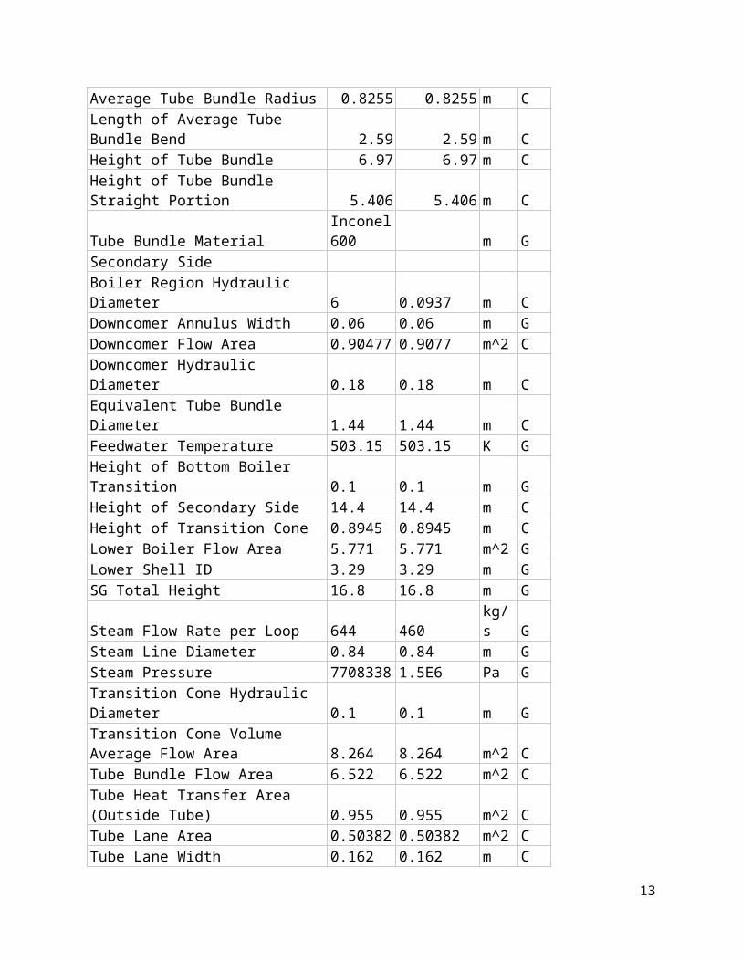
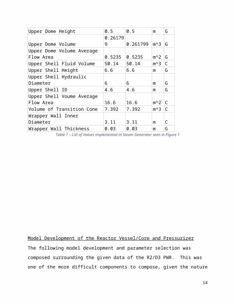
Table 1 – List of Values implemented in Steam Generator seen in Figure 1

Model Development of the Reactor Vessel/Core and Pressurizer

9

The following model development and parameter selection was composed surrounding the

given data of the R2/D3 PWR. This was one of the more difficult components to compose,

given the nature of its design. There includes in this component a core barrel and a reactor

vessel surrounding it, with a small downcomer area between them. The sample file

reactorCore.inp was used as a starting point in developing this model. To model the heat which

is present through each portion of the reactor, heat structures were aligned as fuel rods, and on

the sides of the core barrel and reactor vessel. In addition, cold and hot leg pipes which are

connected to the left and right sides of the vessel, respectively mimic the flow immediately

coming in and out of the reactor vessel. The inlet and outlet water flow in and out of the cold

and hot leg pipes have temperature and pressure specifications set by Breaks and Fills that

attempt to portray conditions seen in the steam generator model. A pressurizer was connected

to one of the four hot legs to maintain high pressure, such that the water flowing out of the

reactor vessel does not boil while under such high temperatures.

re.

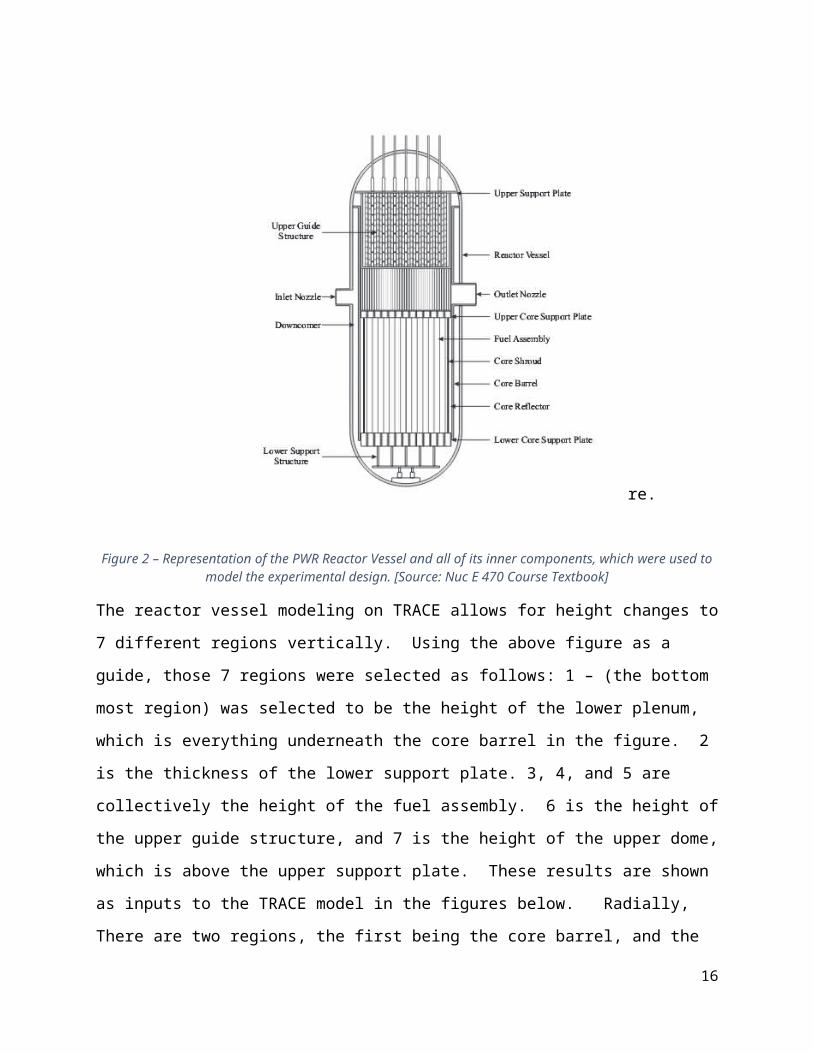
Figure 2 – Representation of the PWR Reactor Vessel and all of its inner components, which were used to model the experimental design. [Source: Nuc E 470 Course Textbook]

10

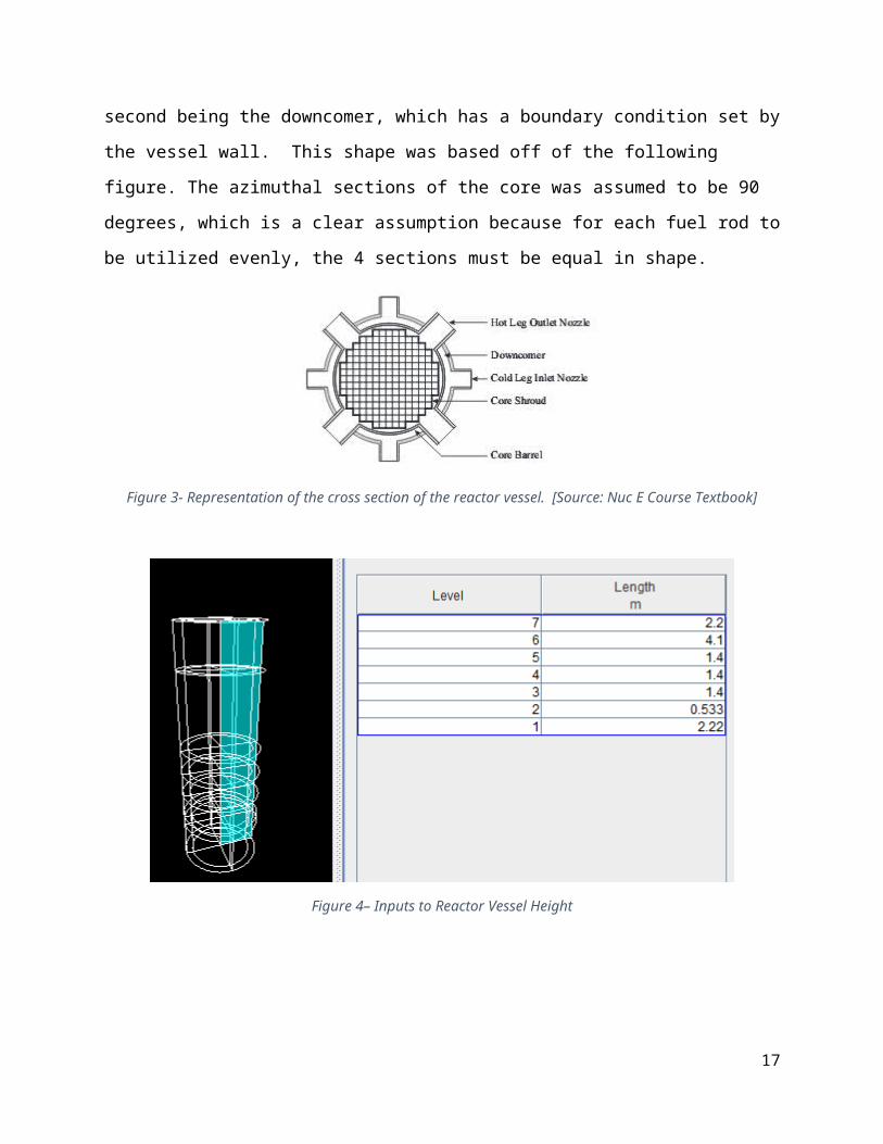
The reactor vessel modeling on TRACE allows for height changes to 7 different regions

vertically. Using the above figure as a guide, those 7 regions were selected as follows: 1 – (the

bottom most region) was selected to be the height of the lower plenum, which is everything

underneath the core barrel in the figure. 2 is the thickness of the lower support plate. 3, 4, and

5 are collectively the height of the fuel assembly. 6 is the height of the upper guide structure,

and 7 is the height of the upper dome, which is above the upper support plate. These results

are shown as inputs to the TRACE model in the figures below. Radially, There are two regions,

the first being the core barrel, and the second being the downcomer, which has a boundary

condition set by the vessel wall. This shape was based off of the following figure. The azimuthal

sections of the core was assumed to be 90 degrees, which is a clear assumption because for

each fuel rod to be utilized evenly, the 4 sections must be equal in shape.

Figure 3- Representation of the cross section of the reactor vessel. [Source: Nuc E Course Textbook]

11

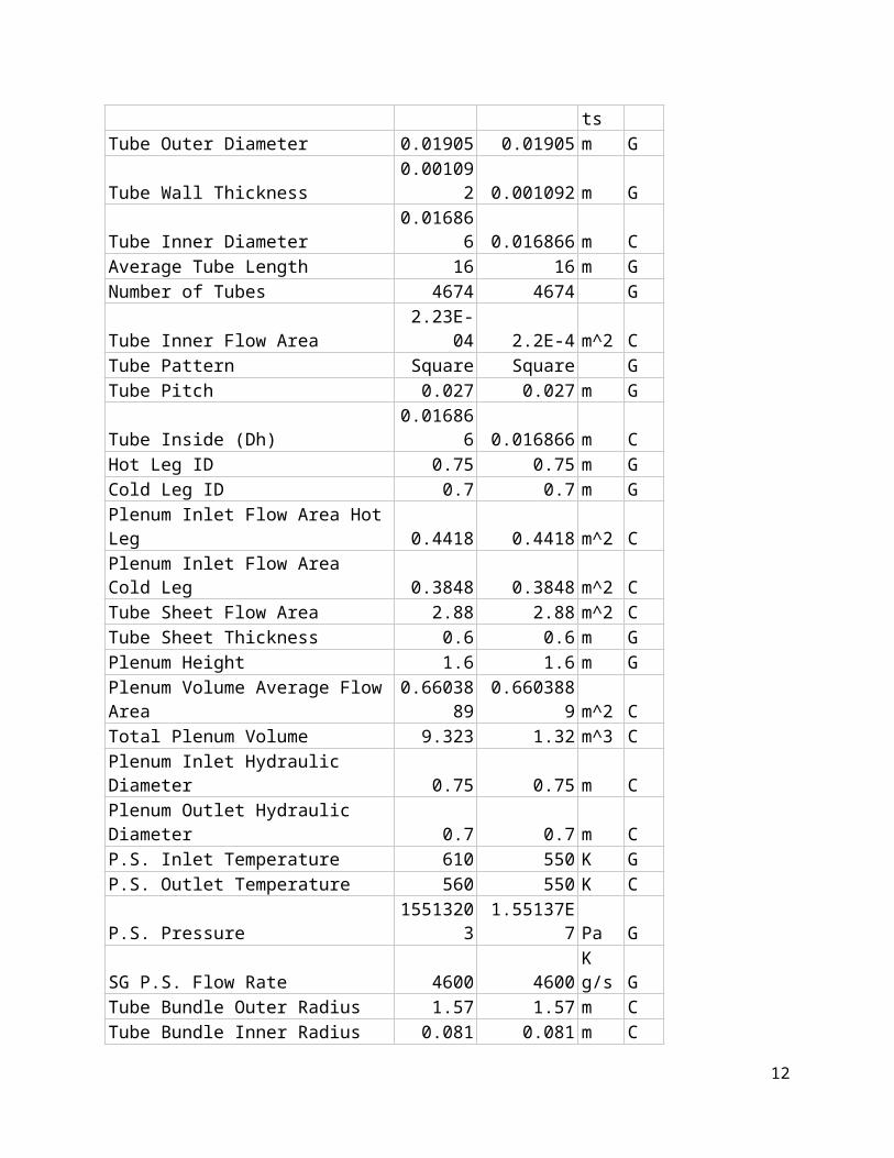
Figure 4– Inputs to Reactor Vessel Height

Figure 5- Input Data on the Reactor Radial Rings

The following Table will assess the parameters that were used as inputs to create the Reactor Vessel.

Parameter As built UnitActive Fuel Length 4 m

Centerline Height of Cold Leg 7.884 mCenterline Height of Hot Leg 7.884 m

Core Barrel ID 3.5752 mCore Barrel OD 3.88 m

Core Barrel Thickness 0.1524 mCore Flow Area 10.02 m^2

Core Fluid Volume 27.060617 m^3

12

Core Hydraulic Diameter 3.574 mCore Thermal Power 3.50E+03 MW_t

Downcomer Flow Area 0.90477 m^2Downcomer Height 8.8 m

Downcomer Hydraulic Diameter 0.18 mDowncomer Width 0.28 m

Efficiency 32 %Equivalent Diameter of Core 2.861 m

Flow Area of Upper Head 13.93471094 m^2Flow Rate Per Hot Leg 4600 Kg/sFuel Assembly Array 17 x 17 N/AFuel Pellet Diameter 0.008001 m

Fuel Rod Cladding Thickness 0.0005588 mFuel Rod Diameter 0.0094996 m

Fuel Rod Gas Gap Thickness 0.0001905 mFuel Rod Lattice Square N/AFuel Rod Pitch 0.0126 m

Height of Lower Plenum 2.22 mHeight of Upper Dome 2.2 mHeight of Upper Head 4.1 m

Height of Upper Support Plate (bottom)

10.75 m

Holes in LCSP 80 mHoles in UCSP 80 m

Inlet Temperature 587 KLCSP Flow Area 5.834310912 m^2

LCSP Fluid Volume 3.109687716 m^3LCSP Hole Diameter 0.3048 m

LCSP Thickness 0.533 mLoss coeff. For LCSP 0.138887817

3N/A

Loss coeff. For UCSP 0.01034427299

N/A

Net Electrical Power 6.71E+02 MW_eNumber of Fuel Assemblies 193 N/A

Number of Fuel Rods per Ass. 264 N/AOutlet Temperature 605 K

Primary Side Pressure 15713203 PaReactor Vessel Height 13.253 M

Reflector Thickness 0.4324 MThickness of Upper Support Plate 0.34 M

Total Assembly Height 4.21 M

13

Total Core Area 2.9559 m^2UCSP Flow Area 5.834310912 m^2

UCSP Fluid Volume 2.522756038 m^3UCSP Hole Diameter 0.3048 m

UCSP Thickness 0.051 mVessel ID 4.44 mVessel OD 4.952 m

Vessel Wall Thickness 0.256 mVolume of Lower Plenum 5.470524 m^3Volume of Upper Dome 15.1976 m^3Volume of Upper Head 52.7834 m^3

Table 2 –Vessel and Core data

The parameters that are in boldface font represent the values that were calculated using the

rest of the parameters (given) and knowledge of PWR geometry. The values that were

calculated were calculated using the equations listed in the appendix.

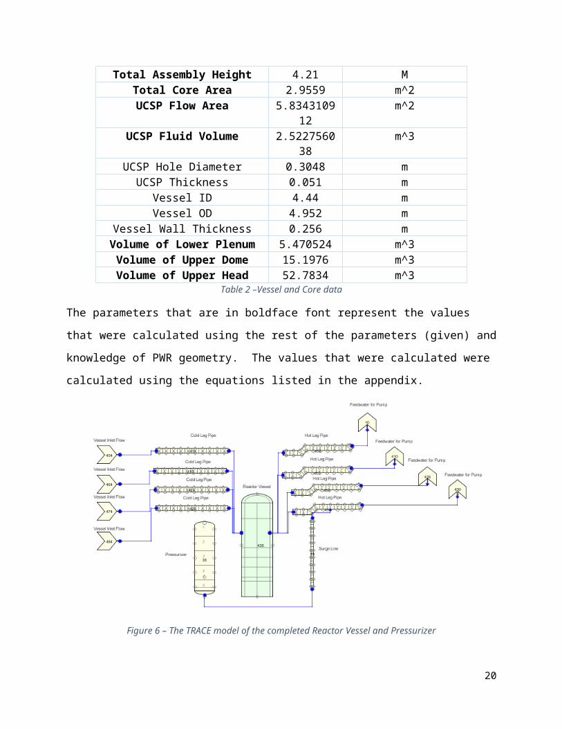
Figure 6 – The TRACE model of the completed Reactor Vessel and Pressurizer

Many changes were made in the development of the core model, for instance, the inlet speeds and energy of the core needed to have slight adjustments following many attempts to achieve steady state. In several of the attempts to run the reactor, the fuel elements became too hot and therefore power needed to be reduced and pressure needed to be raised, although that will be discussed more in the subsystem results section.

14

The following are the initial conditions for the Pressurizer and the details that went into

developing it. The purpose of the pressurizer is to maintain a high pressure and therefore

keeping the coolant in the liquid phase. This high pressure is maintained by water flowing into

the pressurizer, which is set to be 50% full upon initial conditions, and compressing the gas that

compresses with the rising water level.

Parameter As-Built Values Units

Cold Leg ID 0.7 mHot Leg ID 0.75 mCrossover Leg ID 0.7 mLength of Cold Leg 7 mLength of Hot Leg 8.438 mLength of Crossover Leg 14.6125 mPressurizer ID 2.8 mPressurizer Heater Power 1386000 WSurge Line Length 10 mSurge Line ID 0.3556 mPressurizer Volume 75 m^3Pressurizer Height 12.18 mReactor Coolant Pump Flow Area 0.38465 m^2Reactor Coolant Pump Hydraulic Diameter 0.7 m

Table 3 – Pressurizer, Pump, Surge Line, and Cold, Hot, and Crossover Leg data.

The length of the cold leg was specified to be cold leg diameter multiplied by 10. The hot leg

length was calculated similarly, but this included a 45 degree angle, which can be seen in the

above figure. Pressurizer height was determined by dividing the volume by the given flow area

(derived from inner diameter), assuming that the pressurizer is shaped roughly like a cylinder.

15

Model Development of Pump:

The pump model was pulled from a table of data (listed below) given to us by the instructor. We decided to use pump 3 on our model as it passed our test system and produced a steady state graph at a lower pump speed. The pump was used to drive the coolant flow from the hot leg to the cold leg. This is important to the mode as it helps achieve steady state between our hot leg and cold leg mass flow rates. After implementing the standard data we connected 4 pumps to our systems. The pump was placed between our hot leg and cold leg with a crossover leg consisting of X 90 degree angles and X 45 degree angles. After these pumps were in place, a copy of the pump and each of the pipes were placed between a break and fill to test our system. We set the break and fill to a constant mass flow rate, and set the initial conditions to replicate our steam generator model. This test system can be seen below in figure X. The parameters we used are listed in table X.

Figure 7 – Model of Pump Test system in TRACE

Parameter Given Values As-Built Values Units SourceCrossover Leg ID 0.7 0.7 m GLength of Cold

Leg7 7 m C

Length of Hot Leg

8.438 8.438 m C

Coolant Pump Flow area

0.38465 0.38465 m^2 C

Coolant Pump Hydraulic Diameter

0.7 0.7 m C

RCP MOI 3460 N/A kg-m^2 GRCP Hr 843 N/A m^2/s^2 GRCP Tr 42850 N/A N-m GRCP Q’’’ 5.58 N/A m^3/s G

16

RCP ρr 1000 N/A kg/m^3 GRCP ωr 124.4 N/A rad/s G

Table 4 – Table of Data implemented into coolant pump test section

Turbine Model Development

The turbine that was requested in this particular model only required output results. Therefore, the best and simplest way to go in modeling turbine behavior is to use a set of signal and control blocks.

To model the work done by the turbine, the simple thermodynamic property can be used which states that the work done in a system can be calculated by subtracting term 1: the summation of mass flow out of a system multiplied by the enthalpy of the steam in question from term 2: the same summation of mass flow and enthalpy flowing into a system.

This equation can be modeled by the mathematical expression

˙W=∑¿m h−∑

outm h

To solve for these parameters control blocks were set up to pull information from the steam flowing out of the steam generator boiler on the top edge, right as it leaves into the break. Also, the mass flow rate in and out of the turbine were assumed to be equal, because the efficiency term of 0.32 will take care of any frictional loss effects during calculation.

The only variable that is not immediately available is hout. This can be found by using the expression:

hout=h¿−η(h¿−hout , s)

Using the SNAP steam tables, based on the inlet temperature and pressure, h in was determined to be 1.56E6. Using the outlet entropy (3.5 Kj/kg –K), and atmospheric pressure as inlet conditions, the hout,s was found to be 1.19E6. Now, using 0.32 as the efficiency variable, we find that hout = 1.072 E6 J/kg.

This was utilized in the following block diagram to solve for turbine work.

17

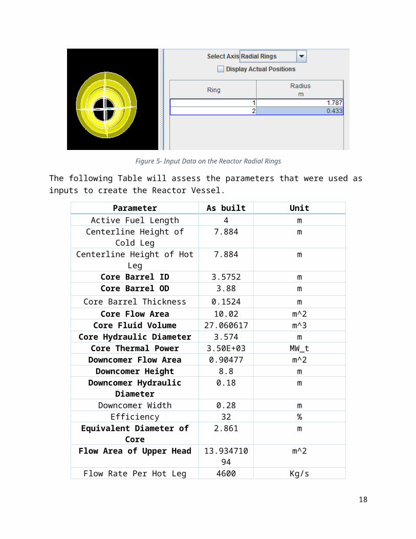
Figure 8 – Control Block diagram for the Turbine Work.

18

Results:

Steam Generator Results:

Before implementing the steam generator into our overall reactor model we created a test system that plugged in the flow rate and temperature expected from our reactor by implementing fills, this can be seen above in figure X. To test the steam generator we looked at the temperature, mass flow rates, and liquid levels in the system. The first thing we analyzed was our Temperature change. Before we looked at the APTplot of our temperature we hypothesized that it should remain steady through the steam generator tube bundles due to the initial conditions set forth by our fill (pressure being constant across and the heat structure being set to the same temperature as our inlet water). As seen in the plot below we were correct in our assumptions.

Figure 9 – Graph of Hot Leg and Cold Leg temperature.

19

The next item we viewed to see if our steam generator was operating in steady state was the mass flow rates of our tube bundles and our inlet by the feedwater nozzle and the exit mass flow rate of the steam generator break. These are illustrated in the below graphs

Figure 10 – Graph of mass flow rate in both Hot Leg and Cold Leg

20

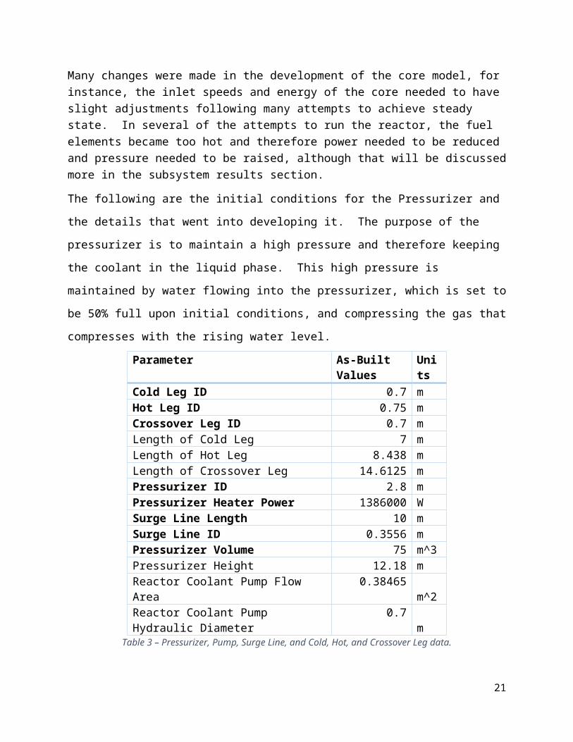
Figure 11 – Graph of Mass Flow Rate into and out of Steam Generator

As see above the mass flow rate in and out of our tube bundles are identical, however they are reflected across the x axis due to the orientation of our pipes (the pipes are reflected across a neutral axis to provide the symmetry that exists in real life steam generators). After reviewing those values we reviewed the inlet and outlet rate of our steam generator and noticed that the outlet rate oscillates right around the inlet rate and determined that the issue could be resolved when the pressure was decreased in our system. We decreased the pressure from 4.85 MPa to 1.5MPa. This produced the state above and showed us that the steam generator was nearly perfect at steady state by itself (more adjustments to our model would be done in our overall model as to save us time and insure an accurate result)

The last piece of interest for us to view if the model is at steady state was the liquid levels of the Downcomer and Boiler. Towards the end of the time we ran the calculation for the value should level out as the boiler consistently produced steam and the downcomer should steadily pump out water. This graph demonstrates the capabilities of our model.

21

Figure 12 – Graph of Liquid Levels in Downcomer and Boiler

From this graph we can see that the model has indeed reached a steady state that is agreeable from a nuclear power plant view.

22

Reactor Vessel and Pressurizer Subsystem Results.

Figure 13 – Exit Mass Flow Rate for Hot Leg – Reactor Vessel

The above figure demonstrates the mass flow out of the hot leg. It is unsurprising that it settles around 4600 kg/s, because that is the speed at which the inlet flows were set.

Figure 14–Cold Leg Exit Temperature – Reactor Vessel

23

The above figure demonstrates how the cold leg temperature remained constant throughout the experiment, because this is the temperature the feedwater is set to.

Figure 15 –Reactor Power – Reactor Vessel

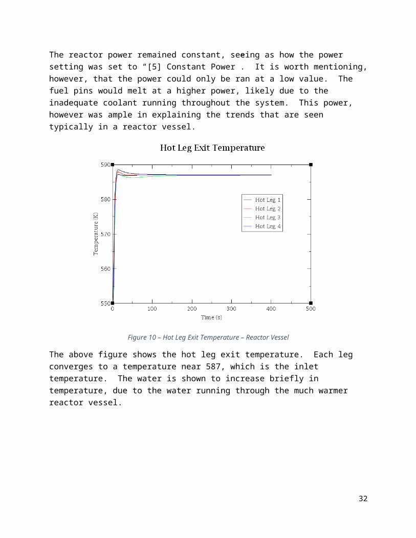
The reactor power remained constant, seeing as how the power setting was set to “[5] Constant Power”. It is worth mentioning, however, that the power could only be ran at a low value. The fuel pins would melt at a higher power, likely due to the inadequate coolant running throughout the system. This power, however was ample in explaining the trends that are seen typically in a reactor vessel.

24

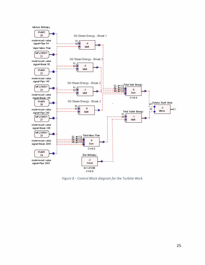
Figure 10 – Hot Leg Exit Temperature – Reactor Vessel

The above figure shows the hot leg exit temperature. Each leg converges to a temperature near 587, which is the inlet temperature. The water is shown to increase briefly in temperature, due to the water running through the much warmer reactor vessel.

Figure 11 – Pressurizer Pressure Difference – Reactor Vessel

25

The above figure addresses the difference in pressure seen in the pressurizer. This is expected, because the pressurizer has components of water and gas, and it would be unusual if the gas had a lower or equal pressure to the liquid, since it is the condensed vapor that creates the high pressure throughout the reactor.

Figure 18- Pressurizer Water Level - Reactor Vessel

The pressurizer water level remains fairly constant throughout the 400 second test. This is very good for the reactor system, because it indicates that there is not much of a deviation from the pressurizer setpoint.

Pump Results:

Inside our test system we adjusted the speed rate of our pump to create the system at steady state. With the rated head being at 124.4 we decided to start with a speed of 100 rad/sec. This produced a flow that was about 600 kg/s below what the expected mass flow was designed to be. We then set forth testing various speeds before finally setting the speed value at 110 kg/s. This produced the coolant flow at the desired. The graphs below show that our model achieved a steady state flow between our hot leg into our cold leg pipes. We then graphed the pressure differences between our inlet and outlet of our pump and the exit pressure of our pipe to see if there was any pressure difference.

26

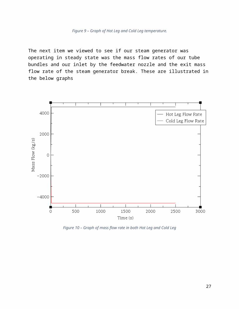
Figure 19- Mass Flow Rate from Hot Leg through Coolant Pump and into Cold Leg

27

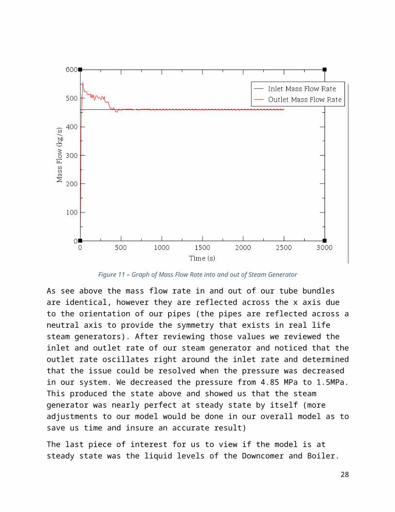
Figure 20- Pressure Levels From RCP into Cold Leg

As these graphs show, the pump system reaches a steady state at the desired mass flow rate with the pump speed set at 110 kg/s. The inlet pressure decreases in the pump but as it leaves the pump it reaches the same pressure as our cold leg exit pressure. The next step is to implement this subsystem 4 times into the overall reactor model. With more connections and point of loss for flow and pressure the flow rate may need to be increased to find the issue.

28

Turbine Results

Figure 21 - Turbine Power

The turbine work seen here is a result of the control block diagram that was derived and explained earlier in this report. It considered the inlet and outlet enthalpies and mass flow rates that were measured at the top of each steam generator. This is the major connection to the turbine that was never physically modeled through TRACE. This figure implies that the Turbine produces around 5.2 gigawatts, which is incredibly unlikely, seeing as how the reactor has a total power of 3.5 gigawatts. That being said, the issue here could have been the lack of efficiency that went into the calculation. If the turbine is 32% efficient, the turbine can only produce a maximum of 1.632 gigawatts, which is much more reasonable in this type of engineering situation.

29

Steady State Plant

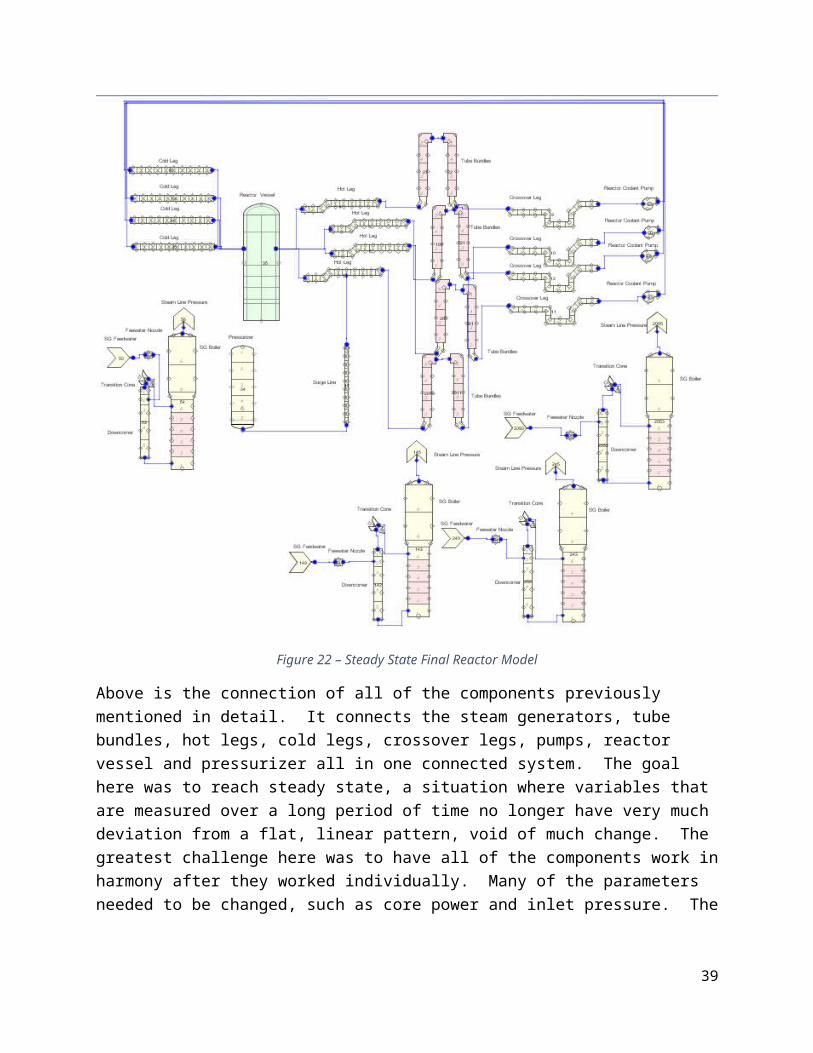
Figure 22 – Steady State Final Reactor Model

Above is the connection of all of the components previously mentioned in detail. It connects the steam generators, tube bundles, hot legs, cold legs, crossover legs, pumps, reactor vessel and pressurizer all in one connected system. The goal here was to reach steady state, a situation where variables that are measured over a long period of time no longer have very much deviation from a flat, linear pattern, void of much change. The greatest challenge here was to have all of the components work in harmony after they worked individually. Many of the parameters needed to be changed, such as core power and inlet pressure. The following figures will display how after changing several of the initial conditions, steady state was approached.

30

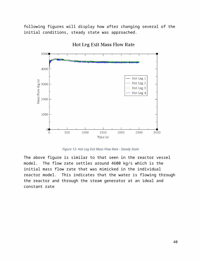
Figure 12- Hot Leg Exit Mass Flow Rate - Steady State

The above figure is similar to that seen in the reactor vessel model. The flow rate settles around 4600 kg/s which is the initial mass flow rate that was mimicked in the individual reactor model. This indicates that the water is flowing through the reactor and through the steam generator at an ideal and constant rate

31

.

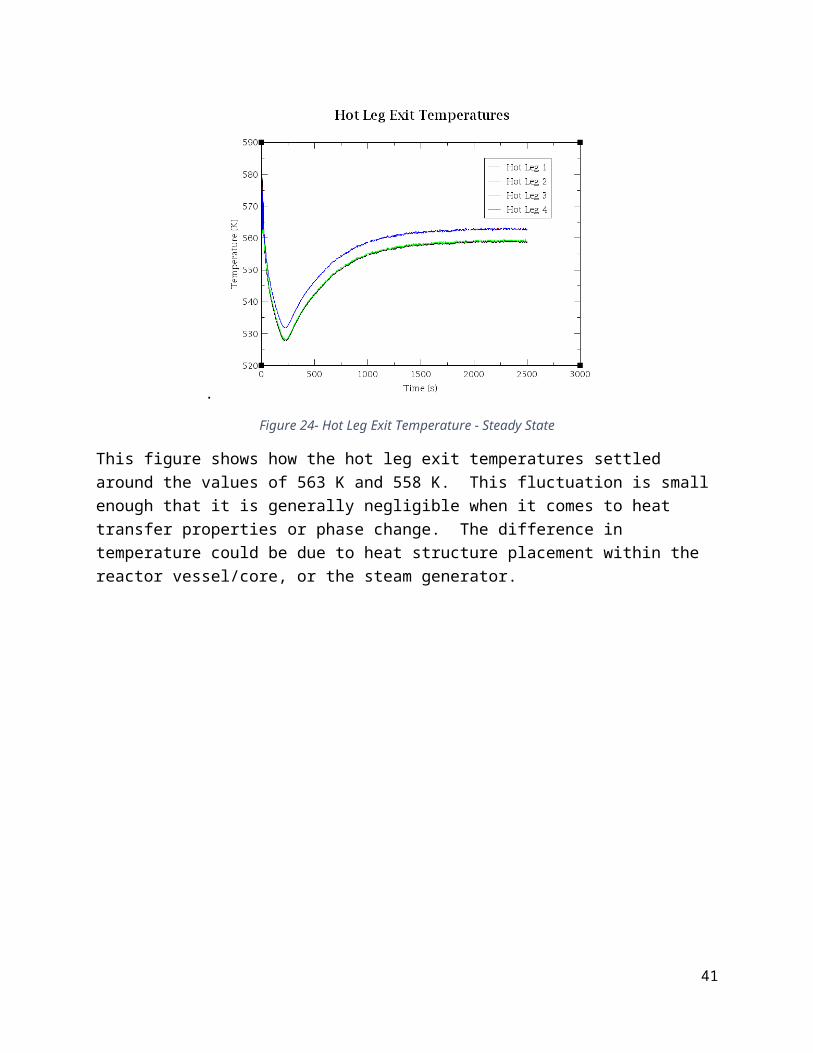
Figure 24- Hot Leg Exit Temperature - Steady State

This figure shows how the hot leg exit temperatures settled around the values of 563 K and 558 K. This fluctuation is small enough that it is generally negligible when it comes to heat transfer properties or phase change. The difference in temperature could be due to heat structure placement within the reactor vessel/core, or the steam generator.

32

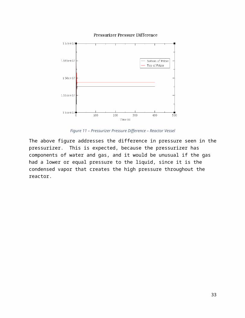
Figure 25- Hot Leg Exit Pressure - Steady State

The hot leg exit pressure was constant for each part of the hot leg. It is slightly lower than the input pressure of 1.56 E 07, however the difference is fairly negligible. The difference is perhaps due to some small inefficiencies in the pressurizer with initial conditions.

33

Figure 13 - Pump Pressures - Steady State

The change in pressure in the in the pumps is indicative of the effectiveness of the pump. The pressure drop of around 0.3 MPa is slightly smaller than expected, but the fact that it is constant implies that slight changes in pump speed would not ruin the pressure drops found throughout the reactor.

34

Figure 14 - Steam Mass Flow out of SGs - Steady State

The mass flows out of the steam generators are all generally following the same trend. The value of mass flow fluctuates between 450 kg/s and 500 kg/s, which is not much unlike the inlet coolant speed of 460 kg/s. This indicates that the steam generator will not be filling up with water, which is good. There is a constant flow of mass in and out at all times.

35

Figure 158 - Steam Temperature - Steady State

The steam outlet temperature fluctuates over time to a range of 495 K and 510 K. This fluctuation is similar to the fluctuation in steam mass flow out of the SG, and therefore the fluctuation in kinetic energy makes sense with a fluctuation in temperature.

36

Figure 169- Water Levels in Boiler - Steady State

As mentioned previously, the mass flow rates in and out of the steam generator are fairly consistent with each other, leading to little to no fluctuation in boiler level. The average level seen is around 1.6 meters.

37

Figure 30 - Cold Leg Exit Temp. - Steady State

The above figure demonstrates a small fluctuation in cold leg temperature, that is very similar in shape and degree of fluctuation of the hot leg exit temperature.

Steady state values were not completely perfect in each of the figures presented, however the model behaved well and converged on to small ranges of values. The initial conditions can be altered slightly to create a more steady state, however in the interest of time, this degree of steady state seemed acceptable. Steady state was generally achieved around 1200 seconds. The system tended to operate at a more steady state at lower initial powers, however experienced failures at lower powers as well.

Plant Transient:

With the limited time we had and the issues we ran into we were unable to complete the transient part of this assignment. After reaching what we believed to be steady state we attempted to initiate a restart case and graphically adjust the model to implement a 5% increase in power. After many attempts this proved to be fruitless. We dug further and looking into our trcout.txt file (the standard trouble shooting file we have used for this entire project) we noticed that the system would not converge to steady state. With time short we decided to attempt to initiate the transient in an informal way. This method would be to introduce a control switch that would be fed the real time of our problem and after it reached a time set by

38

us the increase to power would be added into the system. This attempt to introduce the controller proved to be a more troublesome experience than we thought. After many fatal error messages we decided to abandon the implementation of the transient. While this ignores a part of the model that would be critical to a real world application, we believe that with more time and knowledge of this system could solve this issue with minor effort.

While we did not put the transient in we still wanted to have a basic understanding of what would occur. From previous courses we knew that when the power was jumped up the mass flow rate, temperatures and pressures would spike and then approach a new steady state (except for the mass flow rate as this is a set value). Without a working model that can show us the exact spikes this is the best analysis we can offer on this Transient case.

Conclusions:

After performing the analysis of each subsystem and reviewing each parameter and the overall base model, we determined that our model reached a steady state case within our chosen time frame (1200 seconds). While the system SNAP did not tell us that our model was at steady state review of our flow rates, temperatures, and pressures shows us that steady state is obviously only a few steps away, but due to time we were unable to have the complete system running. This led to our transient being omitted from our working model for the reasons list above. This model is useful in showing us how difficult it can be to work with an unfamiliar system and the challenges that will be found as we work through each system and how we can make it the most efficient we can make it.

39

Appendix:

Equations for Steam Generator:

Primary Side

Secondary Side

40

Equations for Reactor Vessel/Core and PressurizerCore Barrel ID: DCBI =DCB

O −2∗tCB

Core Flow Area: Acore=π4∗D I

CB2

Core Fluid Volume: V Core=Acore∗LAs

Core Hydraulic Diameter:Dhcore=4∗Acore

PwetCore Thermal Power: Calculated from the power.exe file given to us.Downcomer Flow Area: ADC=

π4∗W DC

2

Downcomer Height: H DC=4+tLCSP+tUCSPDowncomer Hydraulic DiameterEquivalent Diameter of Core¿( Acore

π )12∗2

Flow Area of Upper Head: AUH=0.9∗(DRVI

2 )2

∗π

Fuel Pellet Diameter: DPel=Dfuel rod−2∗thicknesscladding−2∗GasGap Height of Lower Plenum: IDVessel

2

41

Height of Upper Dome: IDVessel

2Inlet Temperature: Found from Steam GeneratorLCSP Flow Area: ALCSP=

π∗(Holes )∗DLCSP2

2LCSP Fluid Volume: V LCSP=ALCSP∗tLCSP

Loss coeff. For LCSP: K LCSP=(1− ADC

ALCSP)2

Loss coeff. For UCSPKUCSP=(1− Acore

AUCSP)2

Net Electrical Power: Qe=Qth∗Eff100Outlet Temperature: ChosenReactor Vessel Height: USCP Thickness + LCSP Thickness + Thickness of the upper support plate + Height of Upper support plate (bottom) + Height of Upper Dome + Height of Lower Plenum Reflector Thickness: tRF=tCB+W DC

Total Core Area: (Core Equivalent Diamete r24

)π

UCSP Flow Area: AUCSP=π∗(Holes )∗DUCSP

2

2UCSP Fluid Volume: V UCSP=AUCSP∗tUCSP

Volume of Lower Plenum: ( 46 )π RVessel ID2

Volume of Upper Dome: ( 43 )∗¿

Volume of Upper Head: Flow AreaUH∗HeightUH

42