Salien cy םם םםםםםם םםםםםםםם םם םםםםPresented by: Avner Gidron Presented to : Prof. Hagit Hel-Or

Welcome message from author
This document is posted to help you gain knowledge. Please leave a comment to let me know what you think about it! Share it to your friends and learn new things together.
Transcript

Saliency
תרצו אם ויזואלית בולטות או
Presented by: Avner Gidron
Presented to : Prof. Hagit Hel-Or
SALIENCY – DEFINITION Saliency is defined as the most
Prominent part
of the picture. In the last lecture Reem has defined it as a part that takes at least one half of the pixels in the picture. We’ll see that it is not always the case, and Saliency has more than one definition.
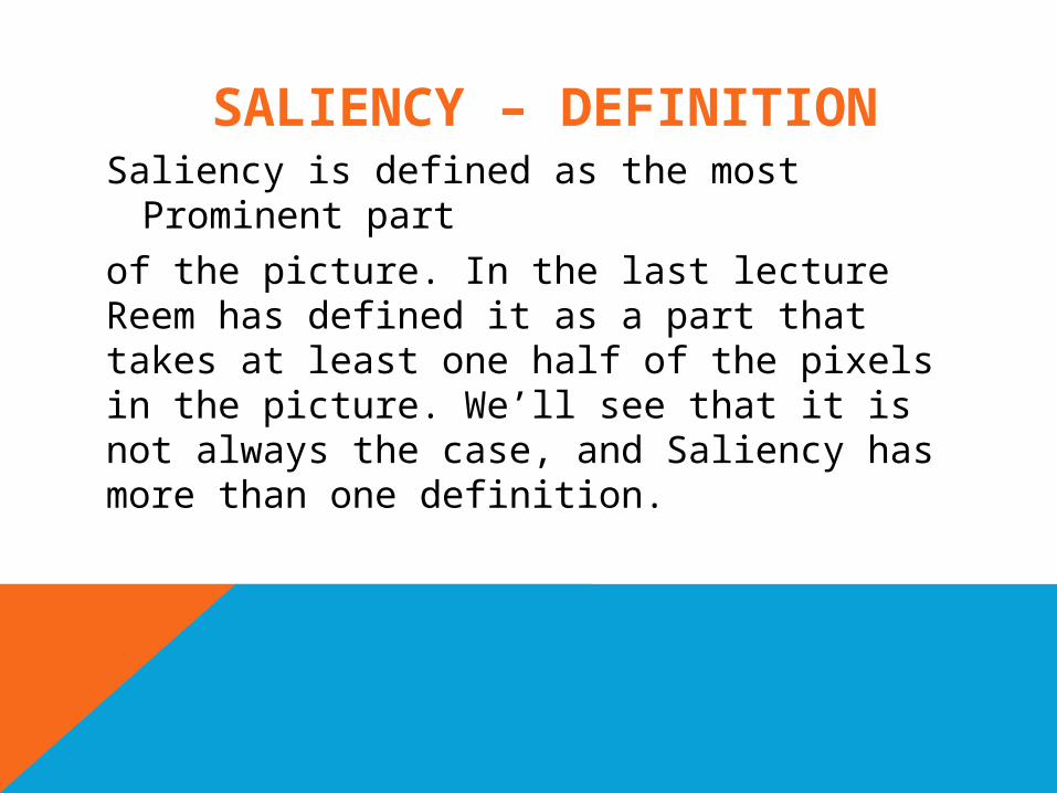
SALIENCY – DEFINITION What is salient here?
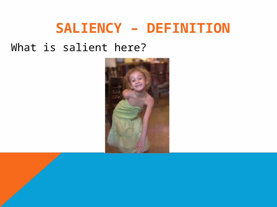
SALIENCY – DEFINITION
Answer:

SALIENCY – DEFINITION Here we can see that although the grass has moreVariance in color and texture the horse is the salient part.
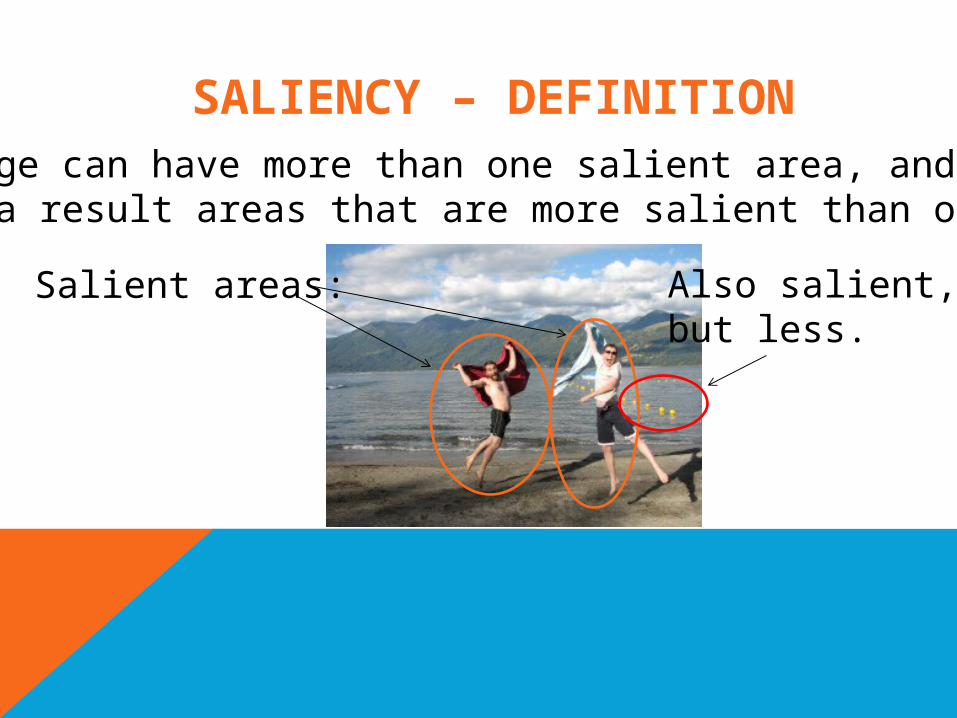
SALIENCY – DEFINITION Image can have more than one salient area, andAs a result areas that are more salient than others:
Salient areas: Also salient,but less.

SALIENCY – DEFINITION Our objective – saliency map:

Sometimes all you need are a few words of encouragement.

How would you divide this picture to
segments?

A possible answer :Two segments:
The swimmer
The background
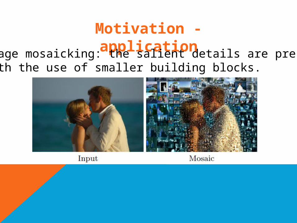
Motivation - applicationImage mosaicking: the salient details are preserved,
with the use of smaller building blocks.
Motivation - application
input Painterly rendering
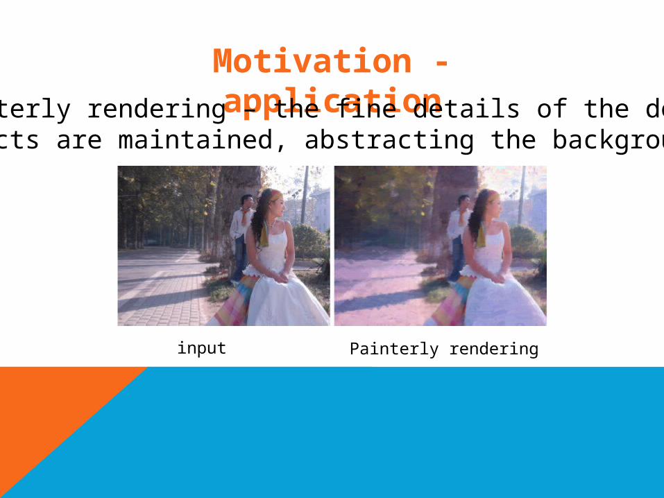
Painterly rendering – the fine details of the dominant objects are maintained, abstracting the background

So, what are we going to see today?
Automatic detecting single objects (Local).
Automatic detecting fixation points (Global).
Global + Local approach.
Explanation on Saliency in human eyes.

Saliency in human eyes
Our eyes detect Saliency by:
Saliency in human eyes
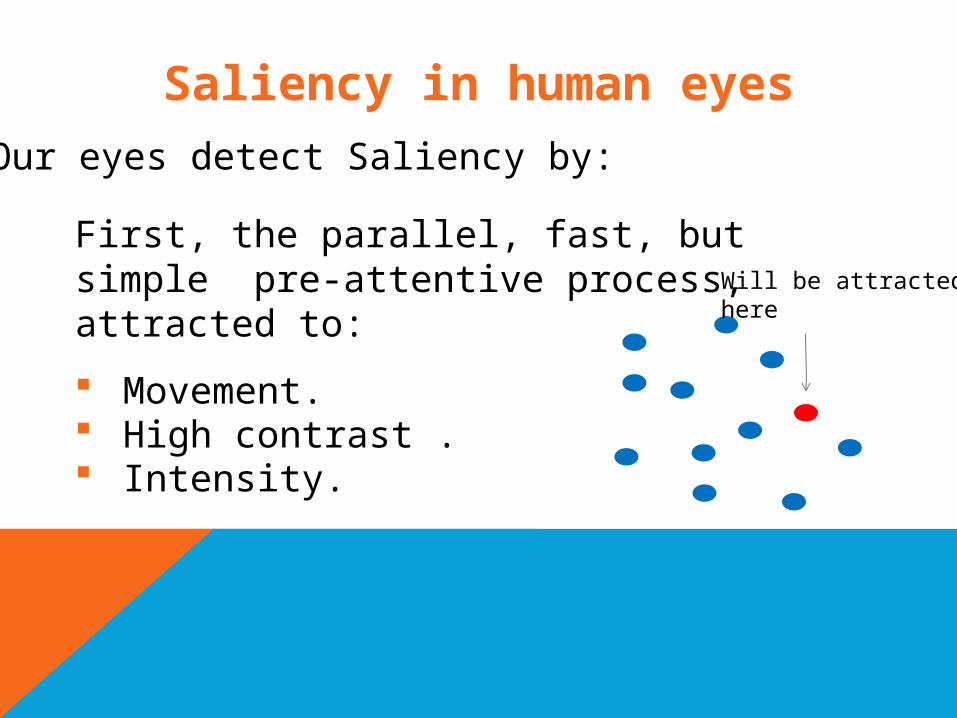
First, the parallel, fast, but simple pre-attentive process, attracted to:
Movement. High contrast . Intensity.
Will be attracted here
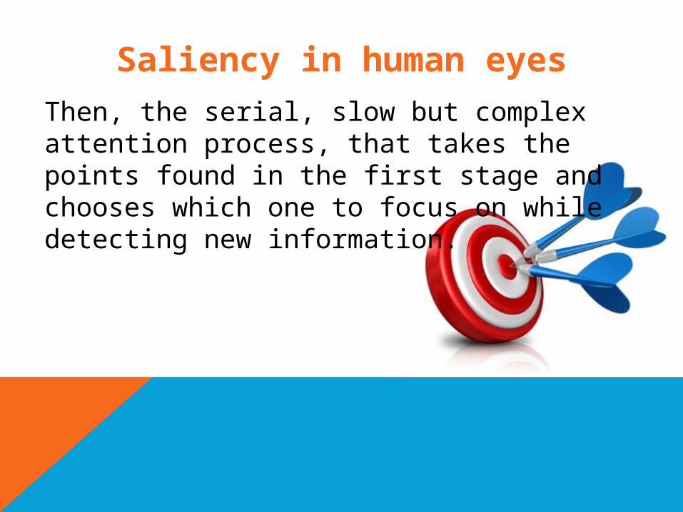
Then, the serial, slow but complex attention process, that takes the points found in the first stage and chooses which one to focus on while detecting new information.
Saliency in human eyes
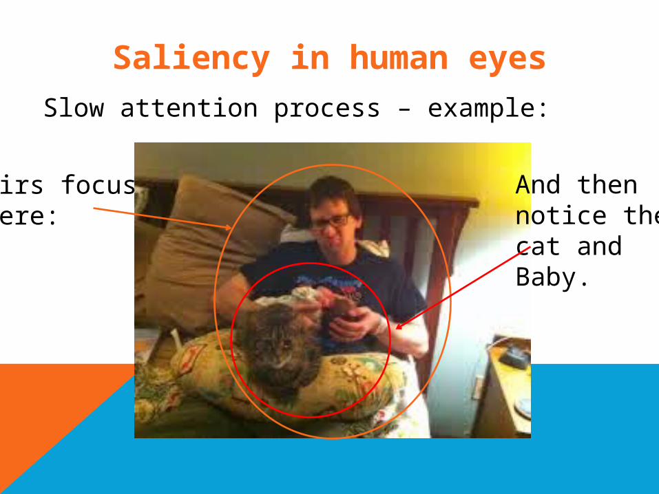
Saliency in human eyesSlow attention process – example:
Firs focus here:
And thennotice thecat and Baby.
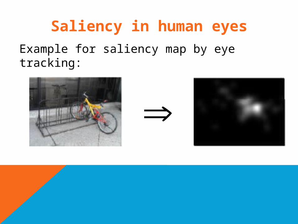
Saliency in human eyesExample for saliency map by eye tracking:

Detecting single objectsOne approach to saliency is to consider saliency as a single object prominent in the imageAn Algorithm using this approach is the Spectral Residual Approach

Spectral Residual ApproachTry to remember from IP lessons.
What did we say that image Consists of?
That’s right!!! Frequencies
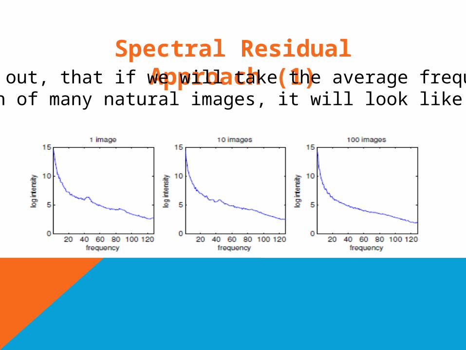
Spectral Residual Approach (1)Terns out, that if we will take the average frequency
domain of many natural images, it will look like this:
Spectral Residual Approach (2)
Based on this notion, if we take the averagefrequency domain and subtract it from a specificImage frequency domain we will get Spectral Residual

ImageTransform = fft2(Image);logSpec = log(1+ abs(ImageTransform));
Spectral Residual ApproachThe log spec. 𝓁 of Image is defined in matlab as:
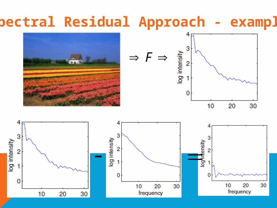
Spectral Residual Approach - example
F

Spectral Residual Approach
2
1 1 1
1 1 11
1 1 1
nh fn
will be defined as a blurring matrix sized :
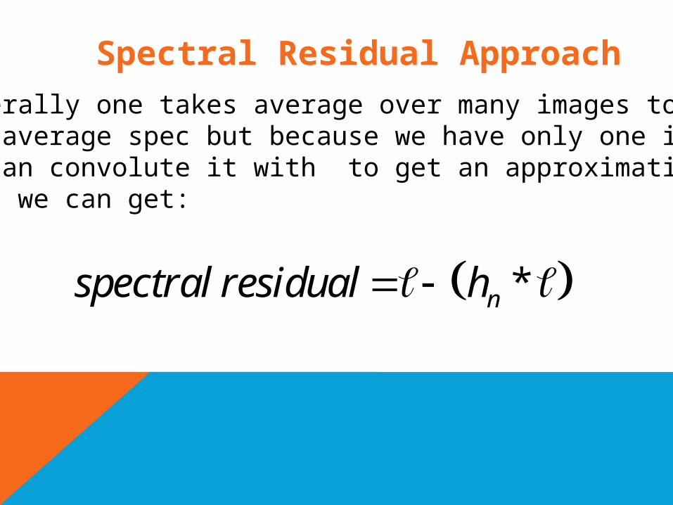
Spectral Residual ApproachGenerally one takes average over many images to getthe average spec but because we have only one imageWe can convolute it with to get an approximation.Then we can get:
*nspectral residual h
Spectral Residual Approach
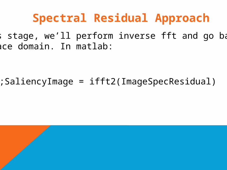
At this stage, we’ll perform inverse fft and go back toThe space domain. In matlab:
SaliencyImage = ifft2(ImageSpecResidual);
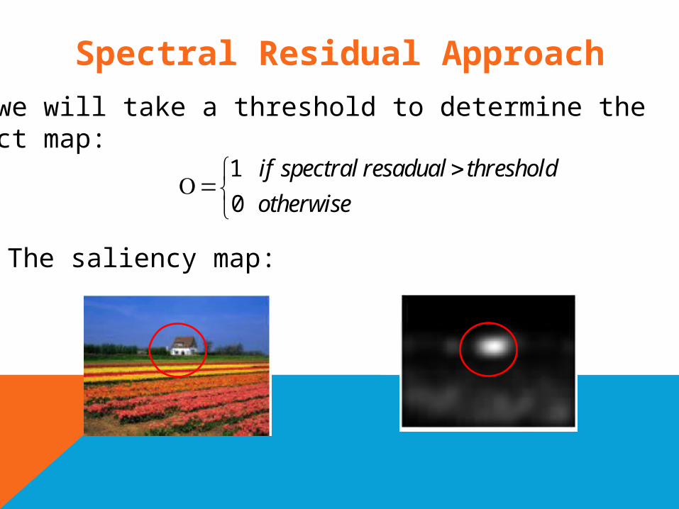
Spectral Residual Approach
And we will take a threshold to determine theObject map:
The saliency map:
1
0
if spectral resadual threshold
otherwise

Detecting fixation pointsAnother approach is to detect points in theimage where the human eye would be fixated on.Not like spectral residual approach, which finds a single point, this approach may find more than onepoint.One algorithm that uses this approach is the onebased on Information Maximization.

Information MaximizationBefore we start, let’s define a few things
Self information:For a probabilistic event, with a probability of p(x),the self information is defined as :
1log log p x
p x
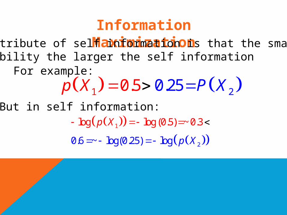
Information Maximization
For example:
1 20.20 5.5 Pp XX
1
20.6
log log (0.5) ~ 0
~ log(0.25) log
.3p
p X
X
But in self information:
An Attribute of self information is that the smaller the probability the larger the self information

Information MaximizationAnother thing we’ll explain is what does Independent
Component Analysis (ICA) Algorithm.
Given a random vectorrepresenting the data and arandom vector representing the components, the taskIs to transform the observed data , using a linearStatic transformation as into maximallyindependent components .
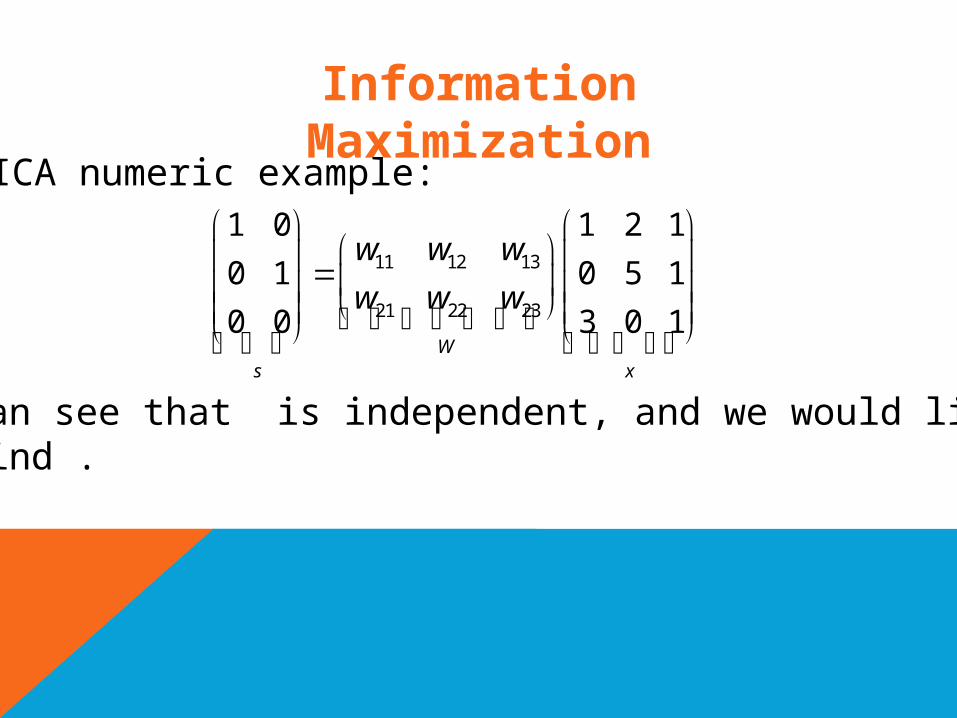
Information Maximization
11 12 13
21 22 23
1 0 1 2 1
0 1 0 5 1
0 0 3 0 1W
s x
w w w
w w w
We can see that is independent, and we would liketo find .
ICA numeric example:

5 1 31 0 1 2 14 2 40 1 0 5 14 3 1
0 0 3 0 17 7 7
s xW
Information MaximizationThe answer:
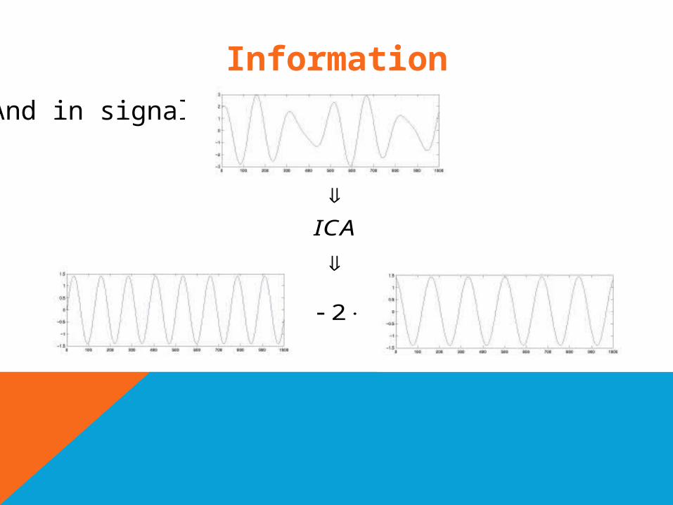
Information MaximizationAnd in signals:
ICA
2
Information Maximization – ICA vs
PCAPCA, Principal Components Analysis- a statistic methodfor finding a low dim. Representation for a large dimensional data.
* Fourier basis are PCA components of natural images

Information Maximization – ICA vs
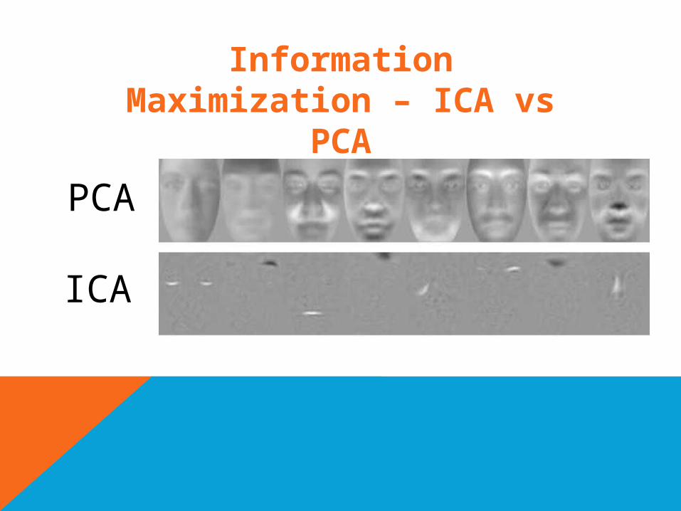
PCAThe different between them is that PCA find his Components one after the other, in a greedy way, findingthe largest component each time, while paying attention to ortogonalty. the ICA works in parallel finding all thecomponents at once, while paying attention to independency.
Information Maximization – ICA vs
PCA
PCA
ICA
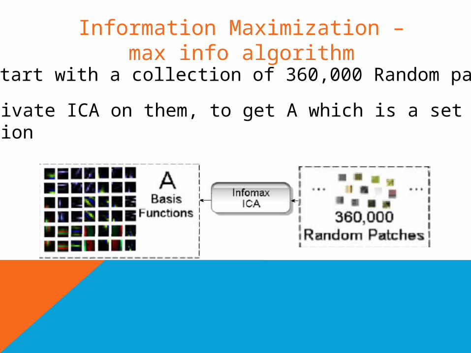
We start with a collection of 360,000 Random patches
and activate ICA on them, to get A which is a set of BasisFunction .
Information Maximization – max info algorithm
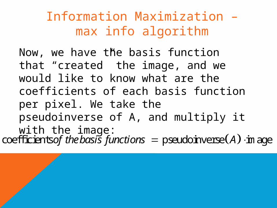
Now, we have the basis function that “created” the image, and we would like to know what are the coefficients of each basis function per pixel. We take the pseudoinverse of A, and multiply it with the image:
Information Maximization – max info algorithm
coefficients pseudoinverse imageof thebasis functions A
1 2
1 1 2 2
, ,...
, ,...N
N N
w w w w
w w w
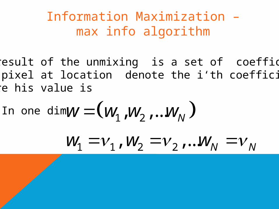
Information Maximization – max info algorithm
The result of the unmixing is a set of coefficients.For pixel at location denote the i‘th coefficient, where his value is:
In one dim:
Information Maximization – max info algorithm
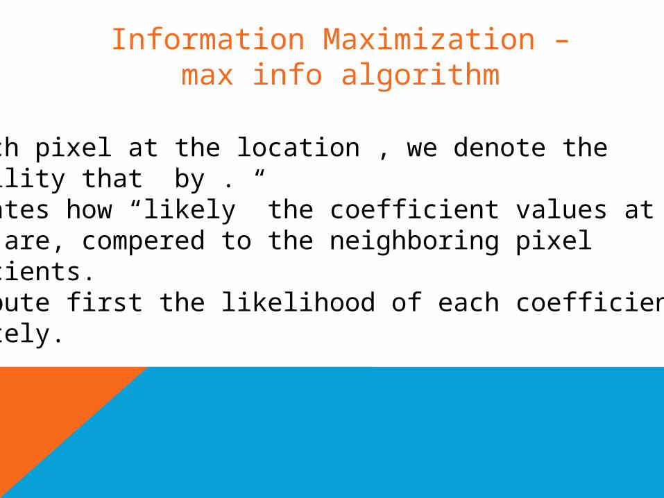
For each pixel at the location , we denote the probability that by . evaluates how “likely” the coefficient values at pixel are, compered to the neighboring pixel coefficients.We compute first the likelihood of each coefficient of separately.

A little bit of math:
2, , , ,
22, ,
,
1,
2
i j k i s t
i j ks t
p w s t e
This Gaussian measures how “stable” are the coefficientswhere 𝛹 is pixel neighborhood, and describes the distance of s,t to j,k.
distance of s,t to j,k .
Similarity of the coefficients
Information Maximization – max info algorithm

Information Maximization – max info algorithm
Pixel j,k
Pixel m,l
We can see that for pixel j,kits coefficients are differentfrom its surround. That’s Why isbig and the prob. is low.On the contrary for pixel m,l, its coefficients are similar toThe ones in its surrounding and that’s way this prob. Is high
, , , ,
2
22, ,
,
1,
2
i j k i s t
i j ks t
p w s t e

Information Maximization – max info algorithm
after computing the likelihood of each coefficient of separately, we denote–
as: 1, , 1, , 2, , 2, , , , , ,...j k j k j k j k N j k N j kp w v w v w v
1, , 1, , 2, , 2, , , , , ,...j k j k j k j k N j k N j kp w v p w v p w v
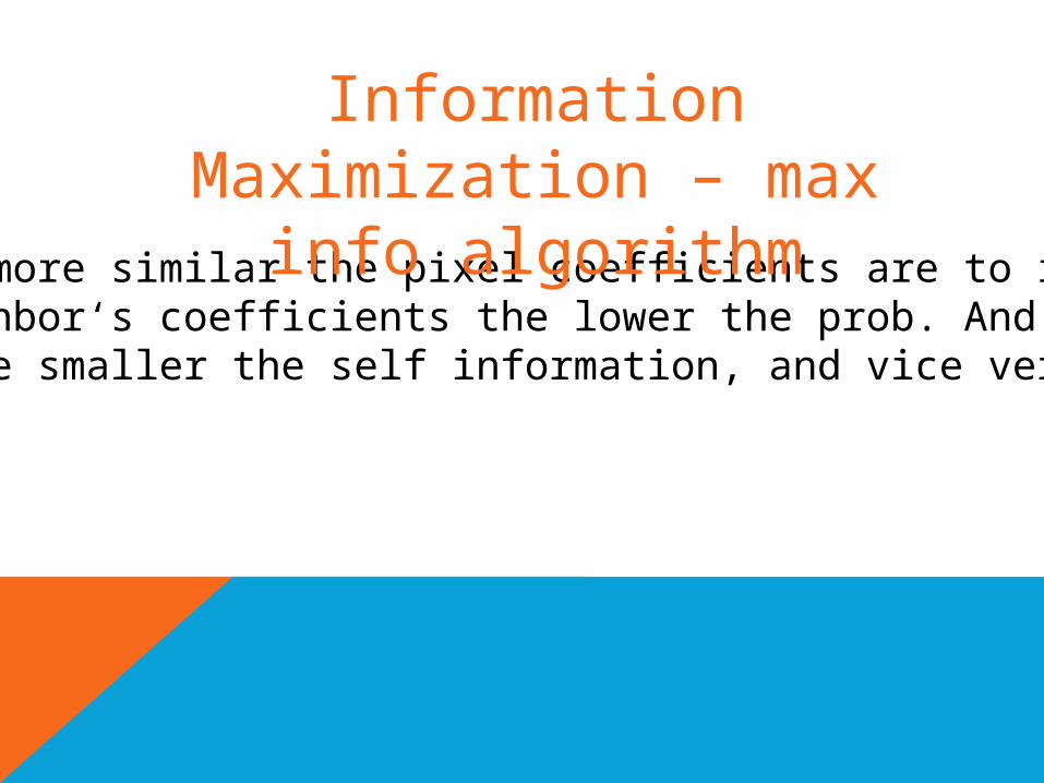
The more similar the pixel coefficients are to it’sneighbor‘s coefficients the lower the prob. And thusThe smaller the self information, and vice versa .
Information Maximization – max
info algorithm

Information MaximizationFor example in the follow image we can see that the
white area will have little “stability” in the coefficients,and therefore small P(X) and so it will have large S.I.We can also notice that that fact go hand in hand withThis area being prominent.
Large selfinformation
Now, we can take the values of the self information and turn it in to a saliency map!!
Information Maximization – max info algorithm
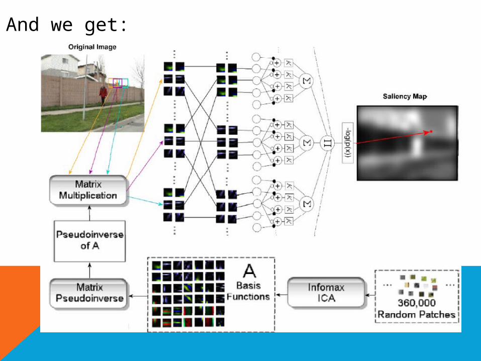
And we get:
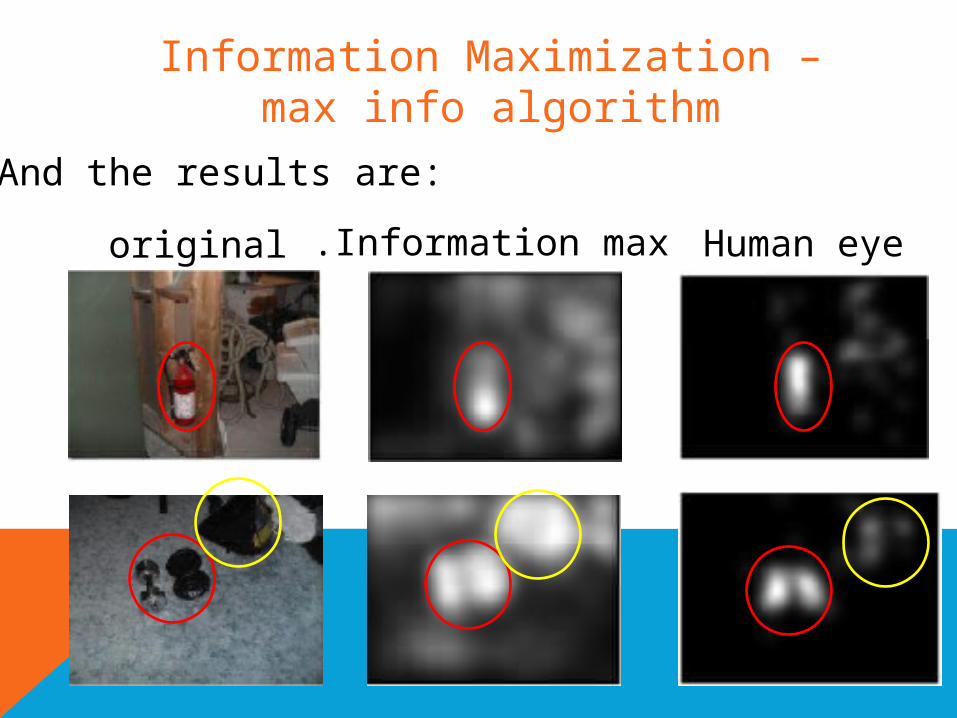
And the results are:
original Information max. Human eye
Information Maximization – max info algorithm

Global + Local approachThis approach uses the information from both the Pixel close surroundings and the information in theEntire picture, because sometimes one of them alone Isn’t enough.
input Local Global
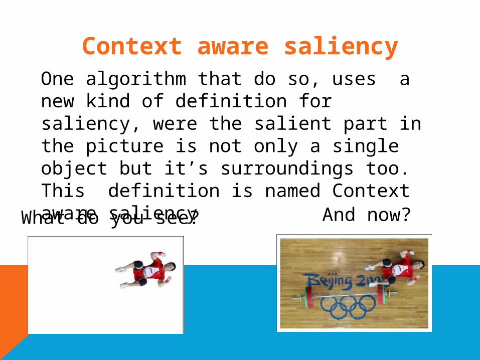
One algorithm that do so, uses a new kind of definition for saliency, were the salient part in the picture is not only a single object but it’s surroundings too. This definition is named Context aware saliency
Context aware saliency
What do you see? And now?
Context aware saliency algorithm (1 )Local low-level considerations,
including factors such as contrast and color
(2 )Global considerations, which suppress frequentlyOccurring features
(3 )Visual organization rules, which state that visualForms may possess one or several centers of attention .
(4 )High- level factors, such as priors on the salient Object location.

A little math reminder:
The Euclidean distance between two vectors X,Y is defined as:
21
, || ||n
i ii
d X Y X Y x y

The basic idea is to determine the similarity of a pixels sized r patch, to other patches’ both locally and globally
Context aware saliency algorithm
as the Euclidean distance between the vectorized patches and in CIE L*a*b color space, normalized to [0,1]

Context aware saliency algorithm
CIE values of(3,4,5)( Y)
CIE values of(5,4,3)( X)
3
2
1
, || || 4 0 4 8i ii
d X Y X Y x y

Context aware saliency algorithm
CIE values of(60,30,90)( Y)
CIE values of(5,4,3)( X)
3
2
1
, || || 3025 676 7569 11270i ii
d X Y X Y x y
Now we can see that pixel i is considered to be salient when is high for all j.
Context aware saliency algorithm
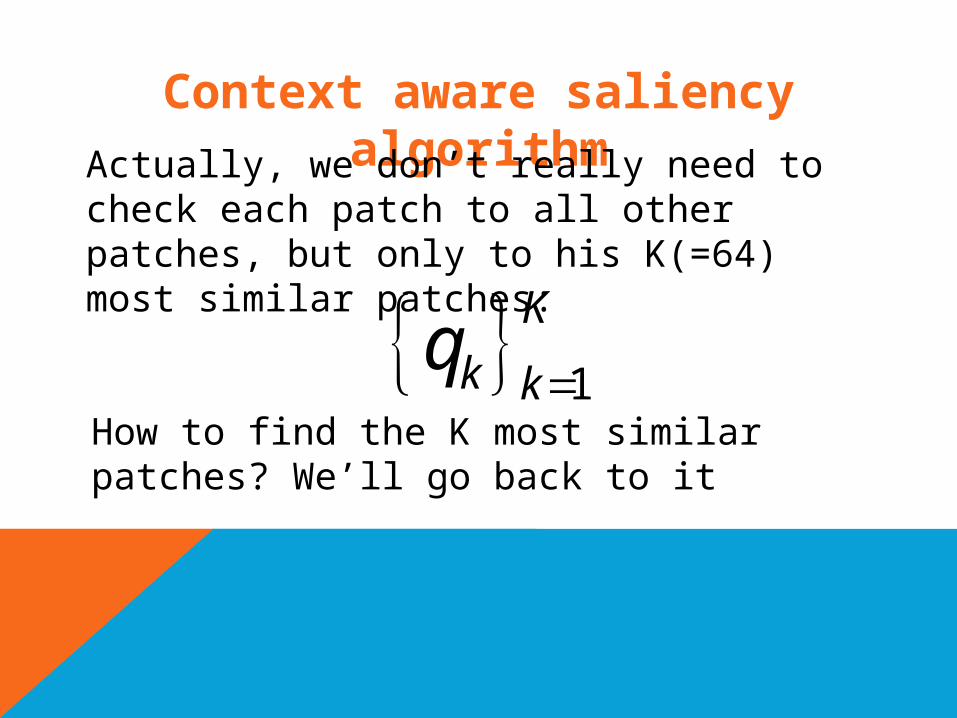
Context aware saliency algorithmActually, we don’t really need to check
each patch to all other patches, but only to his K(=64) most similar patches:
1
K
k kq
How to find the K most similar patches? We’ll go back to it
Context aware saliency algorithmAccording to principle 3, which state that
visualforms may possess one or several centers of attention we define as the Euclidean distance between the positions of normalized to the image dimension.

Context aware saliency algorithm is introduced because as we can notice,
background pixels will have similar patches at multiple scales (pixel i,j). That’s in contrast to salient pixels (pixel l).
Pixel j
Pixel i
Pixel l

Now we can define dissimilarity as:
,
, 11 3 ,
color i ki k
position i k
d p qd p q
d p q
Context aware saliency algorithm

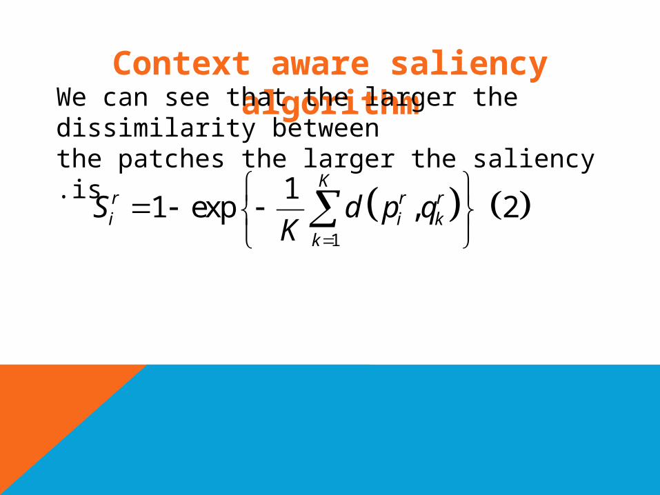
Context aware saliency algorithmNow, because we know that pixel i is
salient if it differs from it’s K most similar patches, we can define single scale saliency value:
1
11 exp , 2r r r
K
i i kk
S d p qK
The equation is summing all the dissimilarity between patch at size r to it’s k most simeller patches,normalized by K.
1
11 exp , 2
Kr r ri i k
k
S d p qK
Context aware saliency algorithmWe can see that the larger the dissimilarity
betweenthe patches the larger the saliency is.

Context aware saliency algorithmA patches size doesn't have to be all in the
same sizes, we can have multiple sizes of patches.
Size
Size
Size r
Context aware saliency algorithm
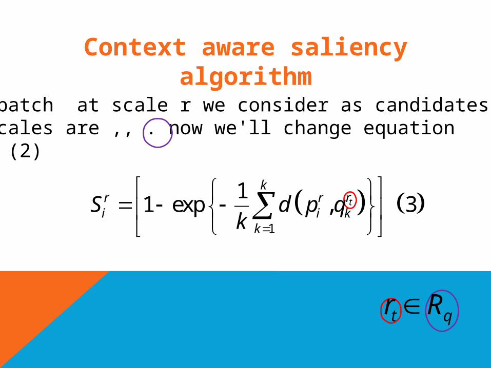
So for patch at scale r we consider as candidates patchesWho’s scales are ,, . now we'll change equation
(2 )to fit:
1
11 exp , 3t
krr r
i i kk
S d p qk
t qr R

Context aware saliency algorithm
And we define the temporary saliency of pixel i as:
14r
i ir R
S SM
For:used
1,...,q MR r r where M is the number of scales
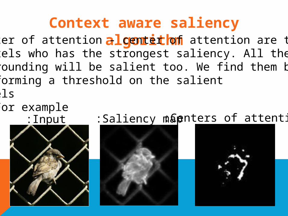
Context aware saliency algorithmCenter of attention - center of attention are the
pixels who has the strongest saliency. All their surrounding will be salient too. We find them bypreforming a threshold on the salientpixels
For example :Input: Saliency map: Centers of attention:

Context aware saliency algorithmOne more thing we want to consider is the
salient pixels surroundings, because as we saw before it may be important to us .
The Euclidean distance between pixel i and the closest center of attention.
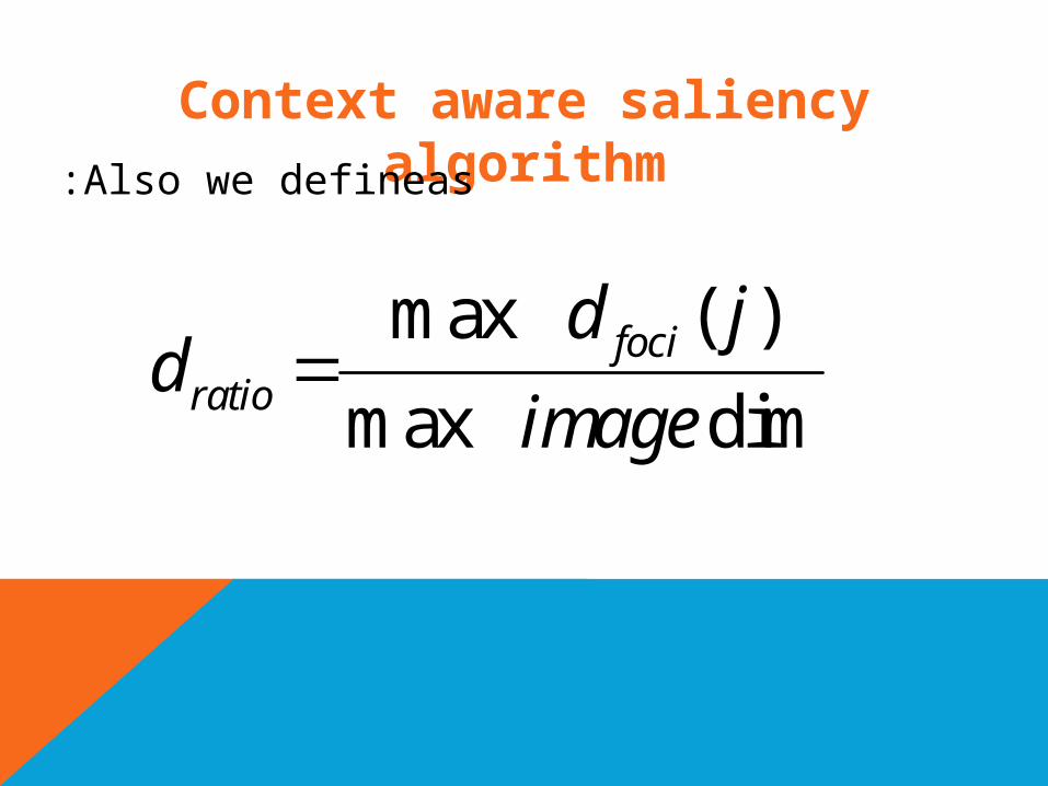
Context aware saliency algorithmAlso we defineas :
max ( )
max dimfoci
ratio
d jd
image
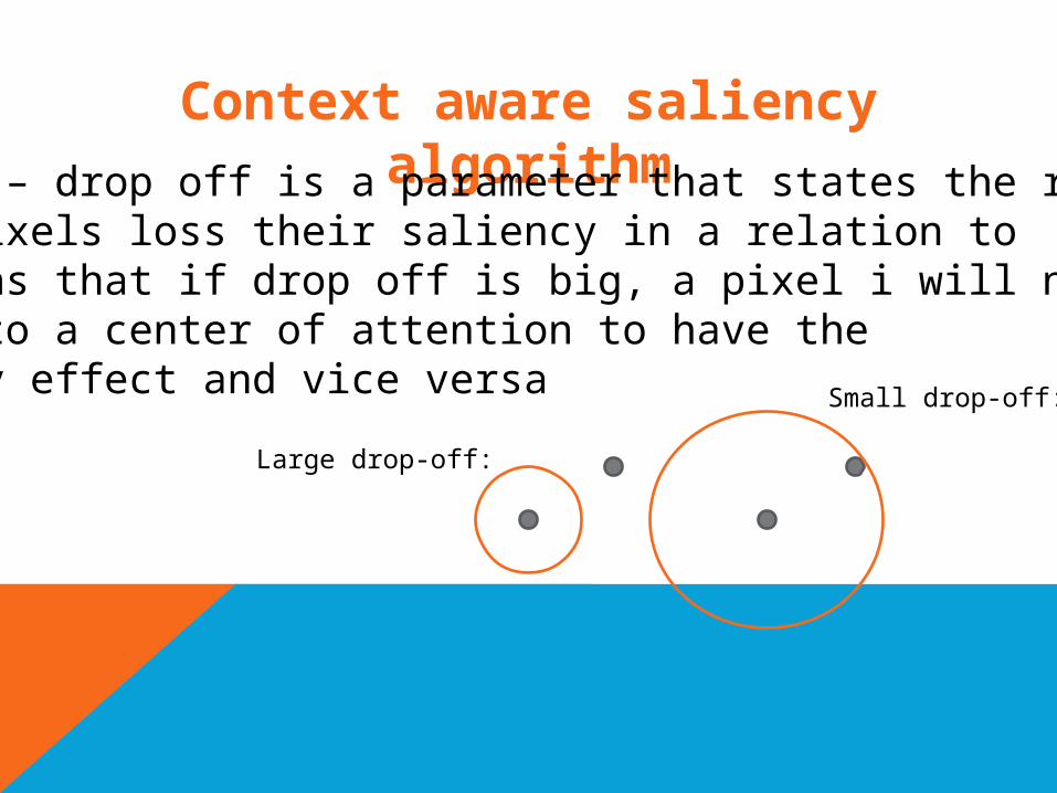
Context aware saliency algorithmDrop off – drop off is a parameter that states the rate
which pixels loss their saliency in a relation to That means that if drop off is big, a pixel i will need to becloser to a center of attention to have the Saliency effect and vice versa.
Large drop-off:
Small drop-off:
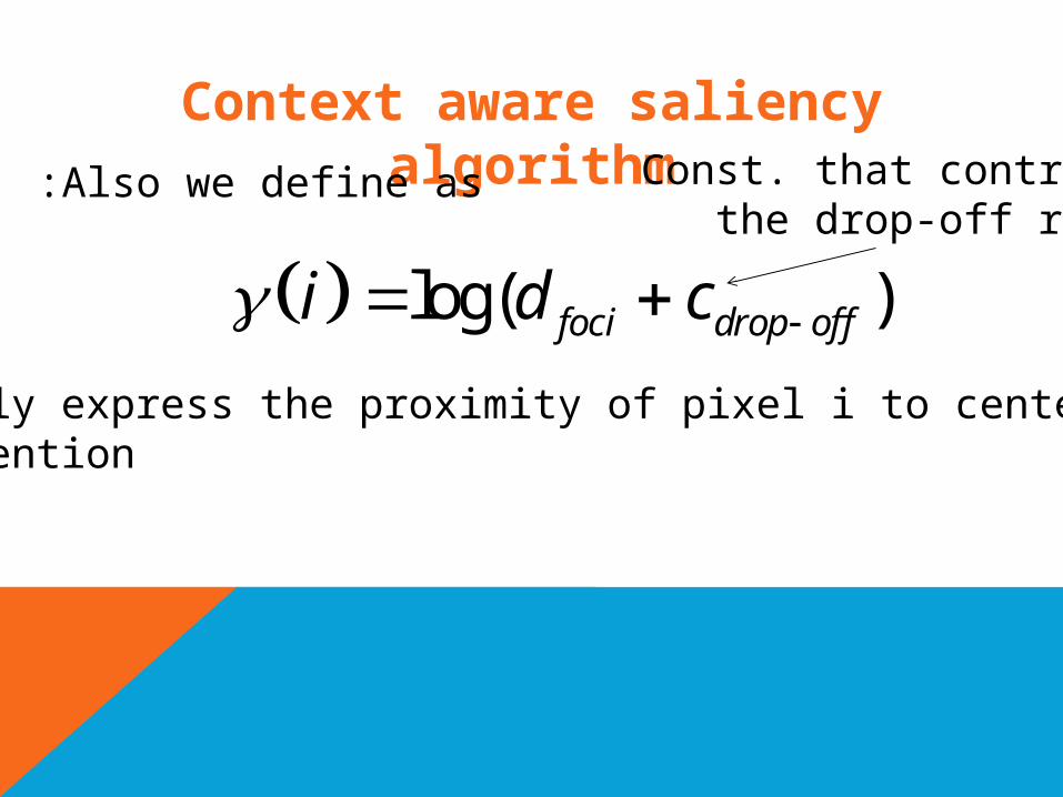
Context aware saliency algorithmAlso we define as :
actualy express the proximity of pixel i to center ofattention .
log( )foci drop offi d c
Const. that controls the drop-off rate

logmax
max dim max log
foci drop offfoci
foci drop off
d cd
IMAGE d c
Context aware saliency algorithm
maxratioi
ii d
i
Also we define as :
To understand it, let’s simplify it:
Constant for all i‘s
That’s why the bigger is, the smaller

Context aware saliency algorithmDon’t panic!! it’s just their way to express the distance of
pixel i to the nearest center of attention, In relation to theentire picture:
max i
iR i
i
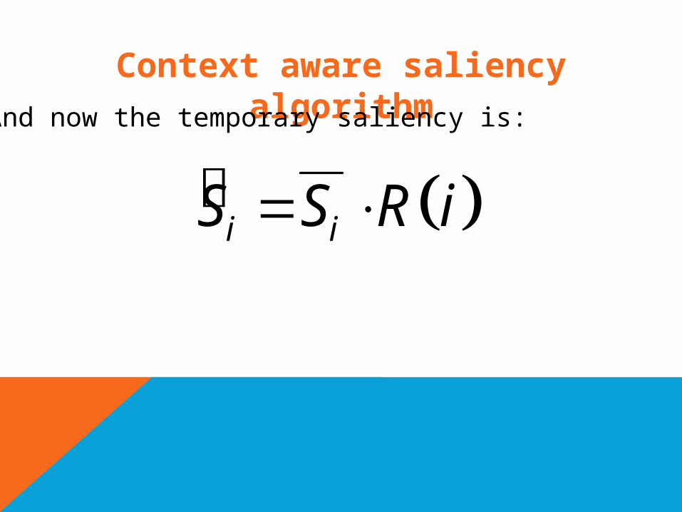
Context aware saliency algorithmAnd now the temporary saliency is:
i iS S R i

Context aware saliency algorithmNow, if you’ll think about how you usually
take pictures, You will notice that in most cases the prominent object :Is in the center of your image
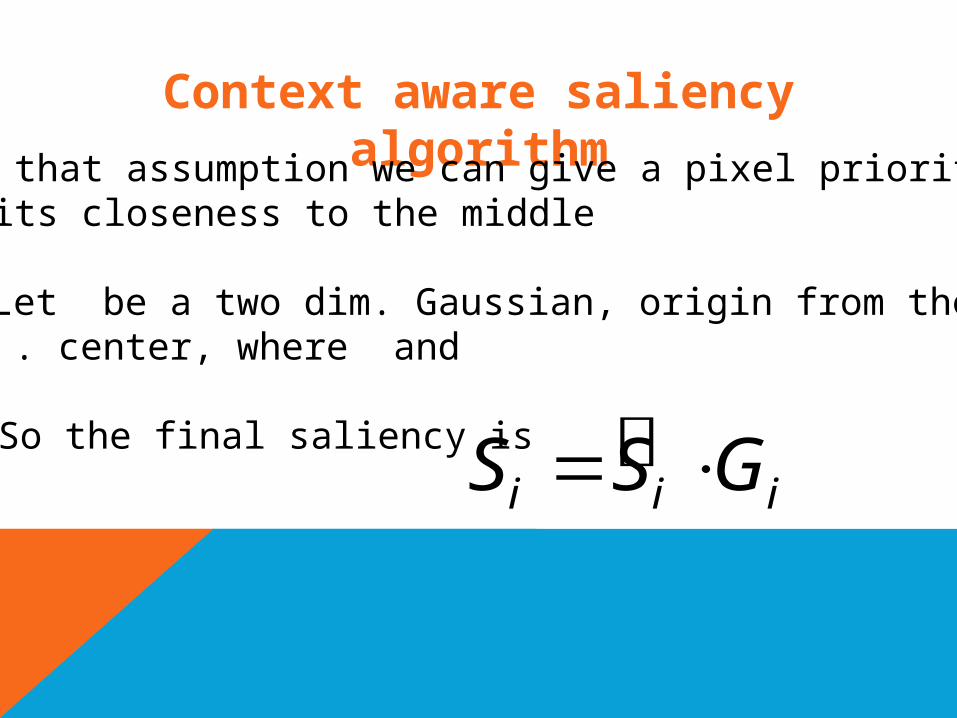
Context aware saliency algorithmUsing that assumption we can give a pixel priority based
On its closeness to the middle .
Let be a two dim. Gaussian, origin from thecenter, where and .
So the final saliency is: i i iS S G

Context aware saliency algorithmHow do we find the K closest patches to a given
patch???
Instead of looking at the real size image, lets build a pyramid

Context aware saliency algorithmThe idea, is to search in a small version of
the image, and then by it focus our search in the real image.
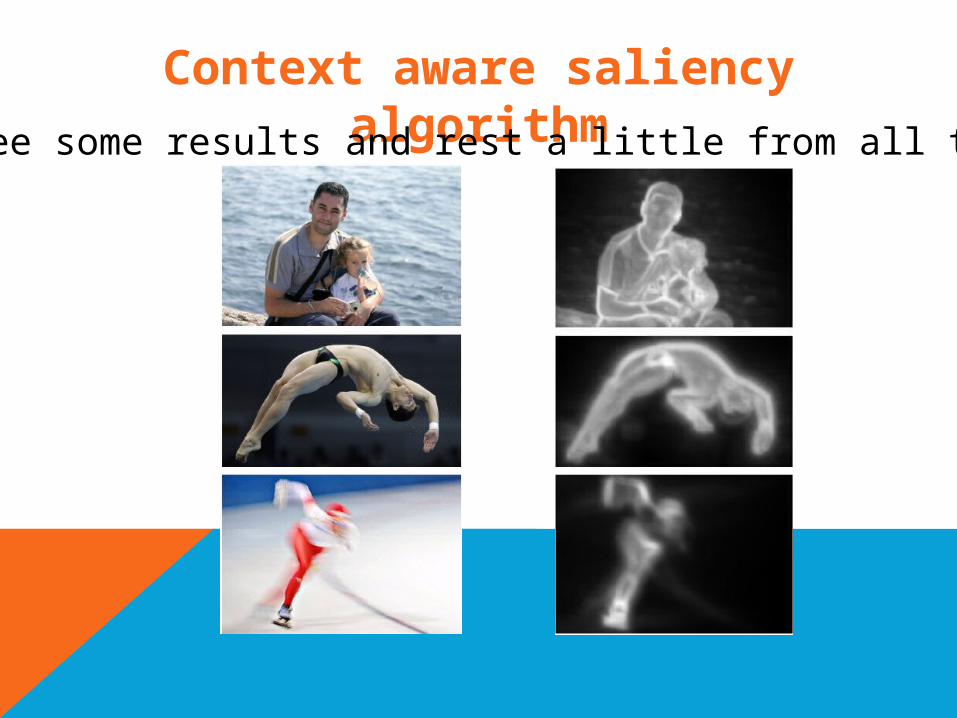
Context aware saliency algorithmLet’s see some results and rest a little from all that math:

A few more Saliency uses:
Puzzle-like collage:
A few more Saliency uses:
Movie Time

Thank you for listening !!!!

REFERENCES
Saliency detection: A spectral residual approach. X. Hou and L. Zhang.In CVPR, pages 1{8}, 2007
Saliency based on information maximization.N. Bruce and J. Tsotsos.In NIPS, volume 18, page 155, 2006.

Saliency For Image Manipulation,"R. Margolin, L. Zelnik-Manor, and A. TalComputer Graphics International (CGI) 2012.
REFERENCES
S. Goferman, L. Zelnik-Manor, and A. Tal"Context-Aware Saliency Detection",IEEE Trans. on Pattern Analysis and MachineIntelligence (PAMI), 34(10): 1915--1926, Oct. 2012.
Related Documents