Presentation 2

Content1. Extrapolation as a tool of forecasting2. Time series components3. Forecasting based on analytical indicators of time series

TOPIC II. FORECASTING BASED ON ANALYTICAL

INDICATORS OF TIME SERIES

Extrapolation is an inference about the future (or about some hypothetical situation) based on known facts and observations.

When you make an extrapolation, you take facts and observations about a present or known situation and use them to make a prediction about what might eventually happen.

For example, we can extrapolate the number of new students entering next year by looking at how many entered in previous years.

What is extrapolation?

1. Extrapolation of trends and patterns is a process of distributing trends and patterns identified in the past and constructing new data points in the future.

Extrapolation of trends and patterns is forecasting technique which uses statistical methods to project the future pattern of a time series data.

Extrapolation types

For example, statistical data on company’s profit for 5 months are given in table below.

If you know statistics on profit through April to August, we might be able to make an extrapolation about profit for the next month. Therefore, extrapolation means that the trend of increasing profit will be the same for the next month as in the past.

Information base for forecasting of trends is one-dimensional time series. For example, statistics on profit through April to August is called one-dimensional time series.

Extrapolation types

2. Extrapolation of causal relationships is forecasting technique which uses statistical methods to construct the multifactor models.

Multifactor forecasting helps to predict a dependent variable from a number of independent variables (i.e. factors).

These factors explain the changes in the development of economic item (data). So, the factors are called independent variables, and the economic item (what do we want to predict) that depends on factors (independent variables) is called a dependent variable.

Extrapolation types

Information base for multifactor forecasting is interrelated time series.

For example, production depends on production costs and demand for products. In this case, production is economic item or dependent variable. Production costs and demand for products are factors or independent variables.

To find the production forecast you need to use specific mathematical tools, for example, regression model.

Table 2 - Statistics on production, production costs and demand for products for 5 months

Extrapolation types

Time series is a collection of observations of well-defined data items obtained through repeated measurements over time.

Separate data of time series is called data points.Time series is the sequence of data points describing the

change of the events, objects or processes at uniform time intervals.

In plain English, a time series is simply a sequence of numbers collected at regular intervals over a period of time.

For example, measuring the level of unemployment each month of the year would comprise a time series. This is because employment and unemployment are well defined, and consistently measured at equally spaced intervals.

Data collected irregularly or only once are not time series.

Time series definition

Spot (point) time series illustrate the data points at every instant of time.

For example: the remnants of the finished product at the first of each month, the value of fixed assets at the beginning or end of the year and etc.

Interval time series illustrate the data points within time interval, such as production for month, quarter and year.

For example: the company’s profit for May is 52 thousand dollars, for first quarter is 208 thousand dollars and for 2013 is 940 thousand dollars.

Time series types

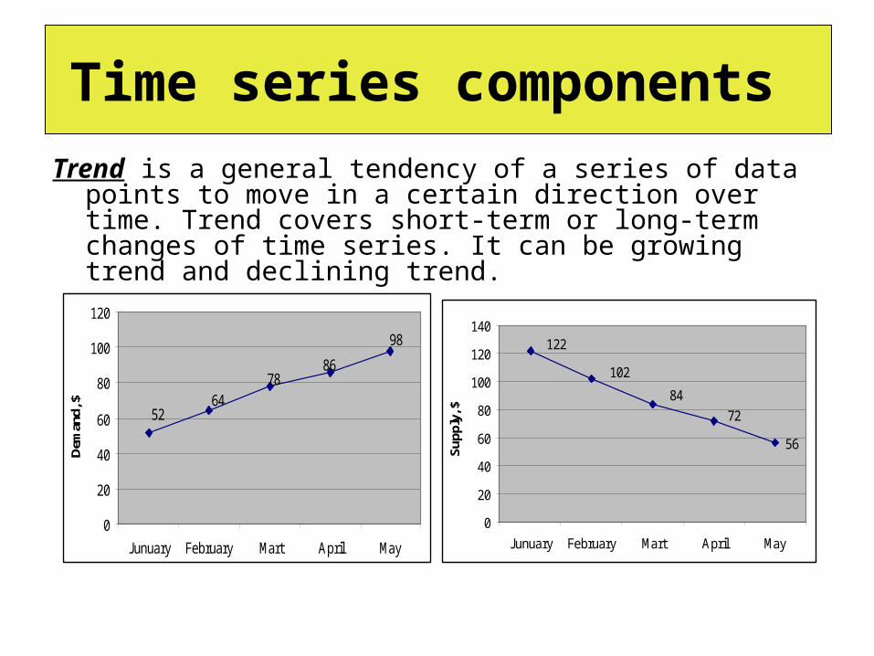
Trend is a general tendency of a series of data points to move in a certain direction over time. Trend covers short-term or long-term changes of time series. It can be growing trend and declining trend.

Time series components

98

8678

6452

0

20

40

60

80

100

120

Junuary February Mart April May

Dem

and,

$

56

122

72

84

102

0

20

40

60

80

100

120

140

Junuary February Mart April May

Supp

ly, $

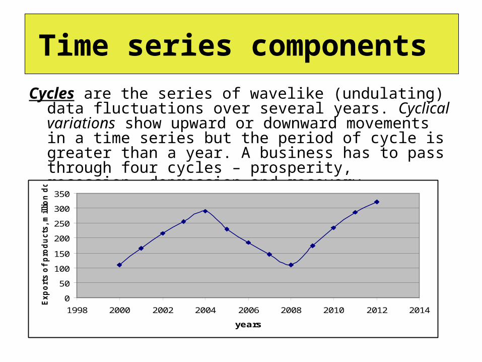
Cycles are the series of wavelike (undulating) data fluctuations over several years. Cyclical variations show upward or downward movements in a time series but the period of cycle is greater than a year. A business has to pass through four cycles – prosperity, recession, depression and recovery.

Time series components

0

50

100

150

200

250

300

350

1998 2000 2002 2004 2006 2008 2010 2012 2014

years

Exp

ort

s o

f p

rod

ucts

, m

illio

n d

ollars

Seasonality is a periodic variation or periodic data fluctuations in the limits of small time intervals: days, weeks, months or quarters (often the term “seasonality” refers to the onset of winter, spring, summer or autumn). The major factors that are responsible for the repetitive pattern of seasonal variations are weather conditions and customs of people.

For example, more woollen clothes are sold in winter than in the season of summer. Regardless of the trend we can observe that in each year more ice creams are sold in summer and very little in winter season.

For example: retail sales tend to peak for the Christmas season and then decline after the holidays. So time series of retail sales will typically show increasing sales from September through December and declining sales in January and February.

Time series components

Random variations or irregular events are the fluctuations and variations caused by unexpected and unusual situations such as introduction of legislation, one-off major cultural or sporting event, strikes, emergencies, civil wars and etc. that cannot be anticipated, detected, identified, or eliminated.

Time series components

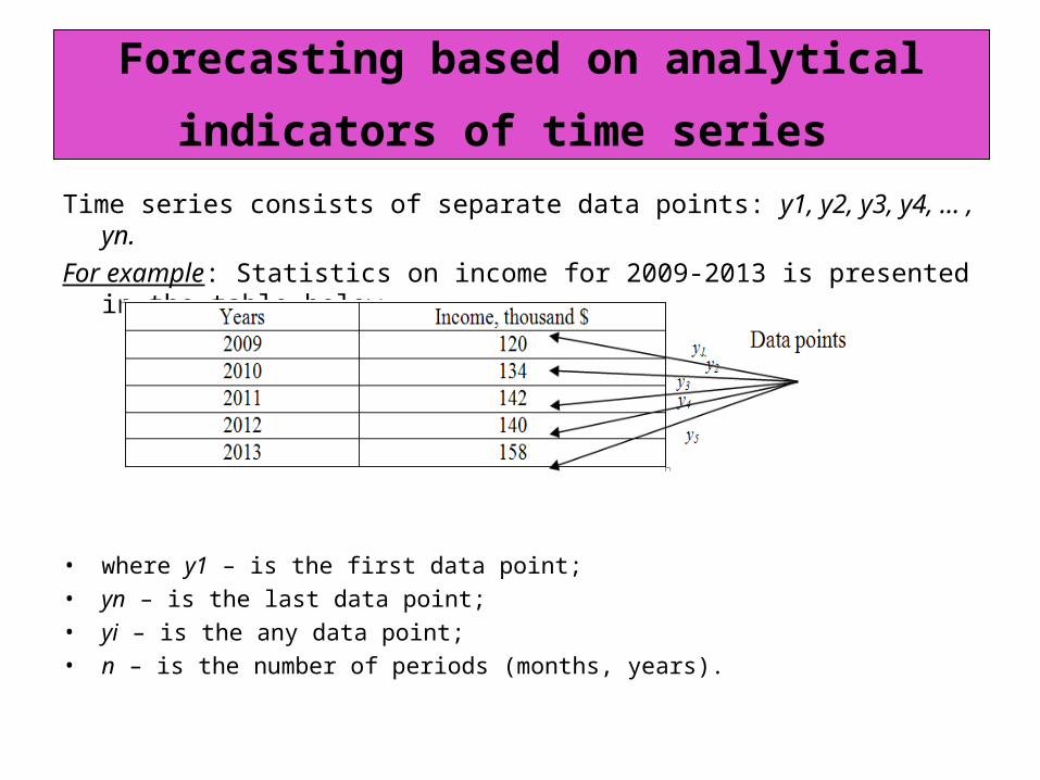
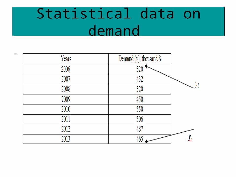
Time series consists of separate data points: у1, у2, у3, у4, ... , уn.

For example: Statistics on income for 2009-2013 is presented in the table below.

• where у1 – is the first data point; • уn – is the last data point;• уі – is the any data point; • п – is the number of periods (months, years).

Forecasting based on analytical indicators

of time series

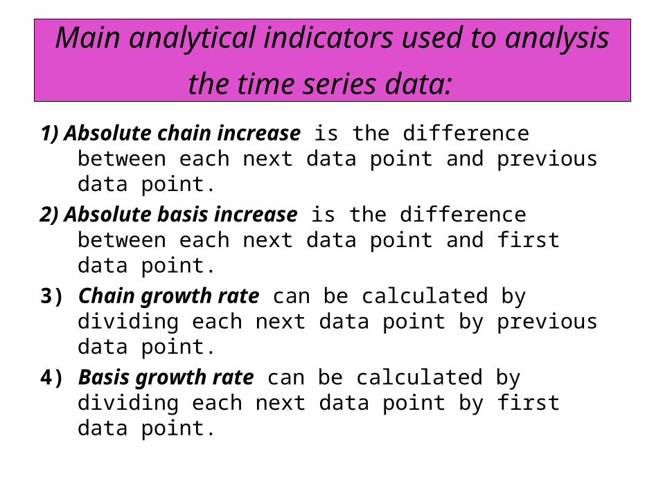
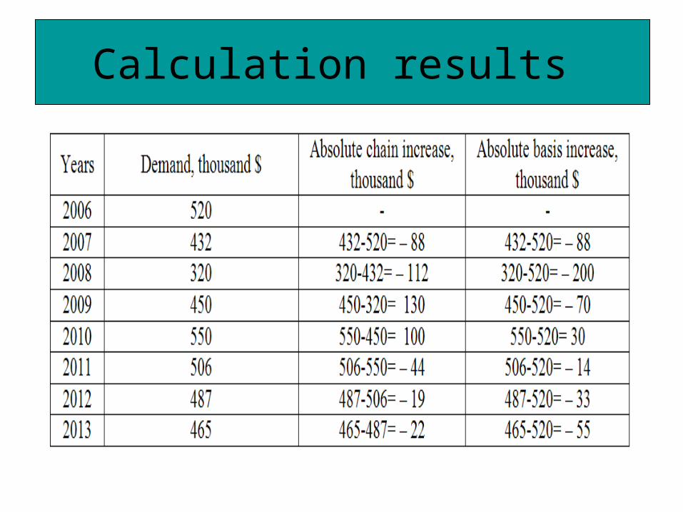
1) Absolute chain increase is the difference between each next data point and previous data point.

2) Absolute basis increase is the difference between each next data point and first data point.

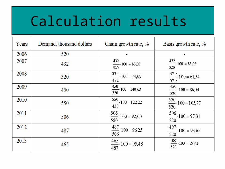
3) Chain growth rate can be calculated by dividing each next data point by previous data point.

4) Basis growth rate can be calculated by dividing each next data point by first data point.

Main analytical indicators used to analysis

the time series data:

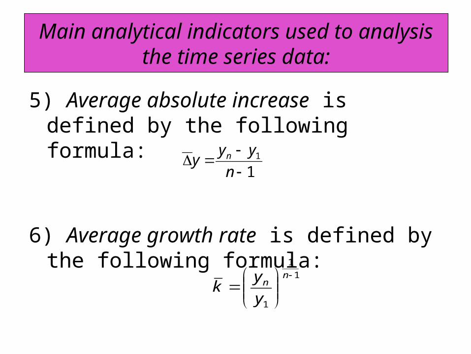
5) Average absolute increase is defined by the following formula:

6) Average growth rate is defined by the following formula:

Main analytical indicators used to analysis the time series data:

11

n

ууу n

1

1

1

nn

y

yk

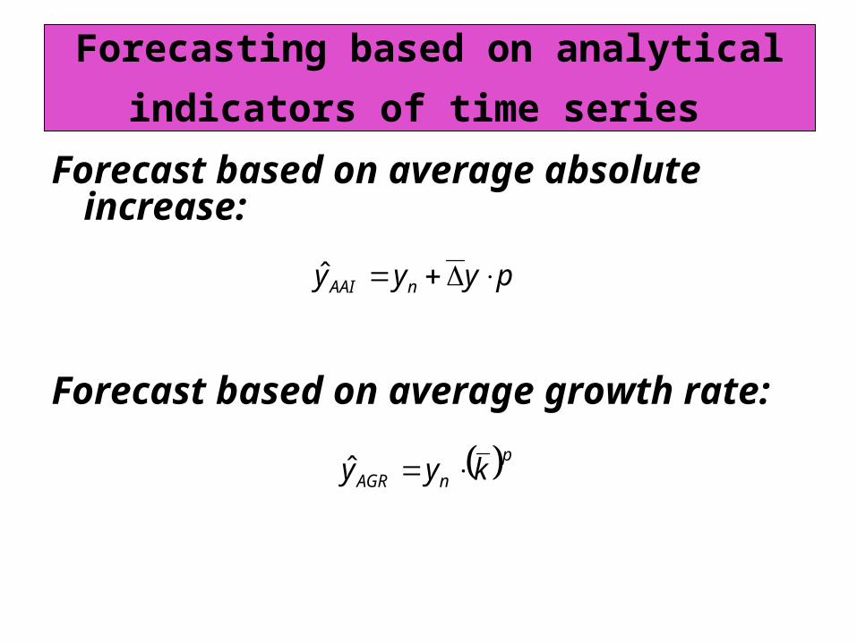
Forecast based on average absolute increase:

Forecast based on average growth rate:

Forecasting based on analytical

indicators of time series

рyyy nAAI ˆ

рnAGR kyy ˆ

Statistical data on demand

Calculation results

Calculation results

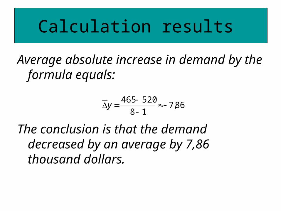
Average absolute increase in demand by the formula equals:

The conclusion is that the demand decreased by an average by 7,86 thousand dollars.

Calculation results

86,718

520465

у

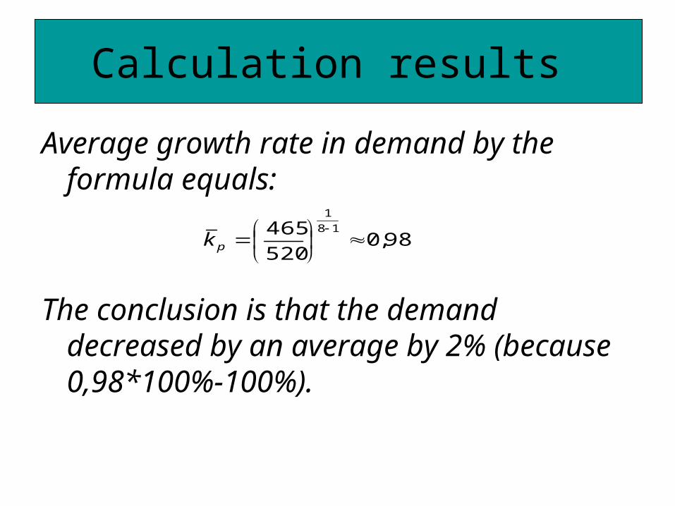
Average growth rate in demand by the formula equals:

The conclusion is that the demand decreased by an average by 2% (because 0,98*100%-100%).

Calculation results

98,0520

465 18

1

рk

for 2014:

for 2015:

for 2016:

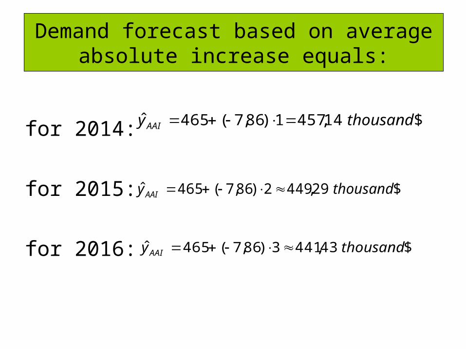
Demand forecast based on average absolute increase equals:

$14,4571)86,7(465ˆ thousandy AAI

$29,4492)86,7(465ˆ thousandyAAI

$43,4413)86,7(465ˆ thousandyAAI

for 2014:

for 2015:

for 2016:

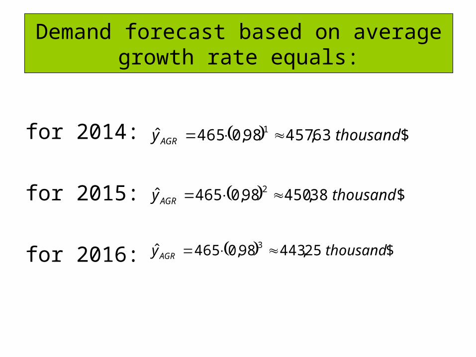
Demand forecast based on average growth rate equals:

$63,45798,0465ˆ 1 thousandy AGR

$38,45098,0465ˆ 2 thousandy AGR

$25,44398,0465ˆ 3 thousandyAGR