Preprocessing of Signals for Single-Ended Subscriber Line Testing

IEEE TRANSACTIONS ON INSTRUMENTATION AND MEASUREMENT, VOL. 55, NO. 5, OCTOBER 2006 1509

Preprocessing of Signals for Single-EndedSubscriber Line Testing

Patrick Boets, Member, IEEE, Tom Bostoen, Leo Van Biesen, Senior Member, IEEE, and Thierry Pollet

Abstract—A preprocessing algorithm is proposed to visualizethe time-domain one-port scattering parameter of a subscriberline measured at the Central Office. To overcome the high lineattenuation and the mismatch between the line and the mea-surement instrument, a preprocessing algorithm is developed toobtain numerically the impulse response of the one-port scatteringparameter. The algorithm will search for a quasi-optimal baseimpedance for the scattering parameter; then, it will de-noise andde-alias the impulse response and will provide an estimate for thefirst meaningful significant reflection.

Index Terms—Impulse response, scattering parameter, timealias, time-domain reflectometry (TDR), transmission lines.

I. INTRODUCTION

R ECENTLY, single-ended line testing (SELT) has be-come a new and interesting topic for telecommunication

operators [1]–[9]. These operators perform loop testing forprospection, prequalification, and maintenance purposes. SELTis highly demanded by those operators and specifically by thecompetitive local exchange carriers (CLECs) because they canonly access the line via the xDSL modems [10]. CLECs are notallowed to connect dedicated test heads to the line itself, butby using SELT, it becomes possible to provide a line qualitymeasurement service to customers.

The idea of SELT is to perform measurements at the CentralOffice (CO) only to obtain a reasonable estimate of the sub-scriber line (loop) makeup or to identify the channel capacityin bits per second of that loop. To achieve this and, moreover,to give a prediction of the topology of the subscriber line,the one-port scattering parameter S11(ω) is used [1]. AlthoughS11(ω) contains all the information, the time-domain versionof S11(ω),which is denoted as s11(t), is used to detect peaksin it, which can be viewed as voltage reflections if the loopis excited with a Dirac impulse. These peaks are detected andanalyzed whereafter the loop makeup can be recognized by theloop classification expert system [2]. Due to the diversity andcomplexity of obtaining a correct s11(t) curve and detectingthe features in s11(t), the approach will be multidisciplinary:It includes the one-port measurement, after which, the dataneeds preprocessing before being passed to the loop topology

Manuscript received October 12, 2004; revised May 3, 2006. This work wassupported by the Flemish Institute of Science and Technology (IWT), Belgium.

P. Boets was with the Department of Fundamental Electronics, Vrije Uni-versiteit Brussel, 1050 Brussels, Belgium. He is now with Banama-Telecom,Brussels, Belgium.

T. Bostoen and T. Pollet are with Alcatel Research and Innovation, 2018Antwerp, Belgium (e-mail: [email protected]; [email protected]).

L. Van Biesen is with the Department of Fundamental Electronics, VrijeUniversiteit Brussel, 1050 Brussels, Belgium (e-mail: [email protected]).

Digital Object Identifier 10.1109/TIM.2006.880290

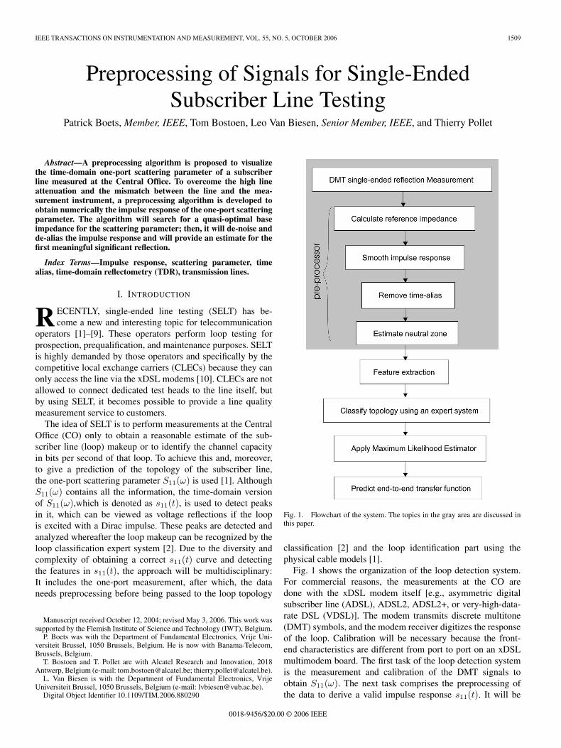
Fig. 1. Flowchart of the system. The topics in the gray area are discussed inthis paper.

classification [2] and the loop identification part using thephysical cable models [1].

Fig. 1 shows the organization of the loop detection system.For commercial reasons, the measurements at the CO aredone with the xDSL modem itself [e.g., asymmetric digitalsubscriber line (ADSL), ADSL2, ADSL2+, or very-high-data-rate DSL (VDSL)]. The modem transmits discrete multitone(DMT) symbols, and the modem receiver digitizes the responseof the loop. Calibration will be necessary because the front-end characteristics are different from port to port on an xDSLmultimodem board. The first task of the loop detection systemis the measurement and calibration of the DMT signals toobtain S11(ω). The next task comprises the preprocessing ofthe data to derive a valid impulse response s11(t). It will be

0018-9456/$20.00 © 2006 IEEE

1510 IEEE TRANSACTIONS ON INSTRUMENTATION AND MEASUREMENT, VOL. 55, NO. 5, OCTOBER 2006

demonstrated that the processed impulse response of a sub-scriber line contains well-pronounced reflections, despite theextremely high attenuation and high dispersion of telephonytwisted pair lines. Because the measurements take place on thenetworks of the operators, it is important that the power spectraldensity (PSD) masks, as proposed by the standards, are not vio-lated. For example, the total power of the excitation signal mustbe below 20 dBm, and excitation in and below the telephonyfrequency band is prohibited if the measurements are done inan ADSL environment [11]. Due to the sparsity of S11(ω),its time-domain counterpart s11(t) cannot be obtained directlywithout some conditioning. It is the task of the preprocessor toadjust s11(t) so that it can be scanned correctly by the featureextraction module. Important features are the delay, height, andenergy of a reflection.

When the features are known, the loop topology can beclassified. For this purpose, a probabilistic reasoning system(Bayes’ belief network) followed by a deterministic rule-basedsystem was used. A classified topology contains the geograph-ical topology (a single line section, cascaded line sections, orcascaded line sections with one or two bridged taps—a bridgedtap is a loop impairment and consists of a short open-endedline that is connected in parallel to the loop) plus the line types(e.g., polyethylene 0.4-mm cable) and an initial estimate of thecorresponding line lengths.

The second last phase (see Fig. 1) in the loop detectionmethod concerns the identification of the S11(ω) measurementwith a model. A maximum likelihood estimator is used for thispurpose. The S11(ω) model uses the Vrije Universiteit Brussel(VUB) cable model to describe the characteristic impedance,attenuation, and dispersion of the line. As initial parameters,the values produced by the rule-based system will be used.

Finally, with the knowledge of the geographical topology andthe estimated model parameters, the power transfer functionfrom the CO to the customer premises can be calculated. Ifthe PSD of the noise at the receiver side is known, using adirect measurement or an estimation of the PSD [12], [13], thenthe channel information capacity can be obtained. For example,Shannon’s capacity formula can be used for this purpose. If abitrate prediction is required that is closely related with the usedxDSL modem technology, then one has to take the filtering, bitloading, analog-to-digital converter (ADC) resolution, codinggain, used tones, etc., into account. For some nonstandardizedparts of a modem, particular information is required from themanufacturer.

As indicated in Fig. 1, this paper gives an in-depth discus-sion of the preprocessing to produce an interpretable impulseresponse s11(t). The output of the preprocessor is the numericaladapted version of s11(t). This output is used by the featureextraction algorithm.

II. MEASUREMENT

An estimation of the power transfer function should beobtained from a test-head-independent quantity. This quantitymust contain fundamental information about the loop but maynot depend on the nature of the excitation signal—if one usesplain time-domain reflectometry (TDR), then the trace depends

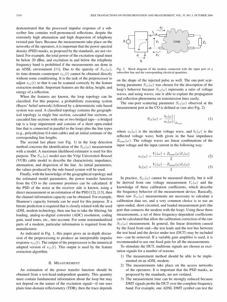
Fig. 2. Block diagram of the modem connected with the input port of asubscriber line and the corresponding electrical quantities.

on the shape of the injected pulse as well. The one-port scat-tering parameter S11(ω) was chosen for the description of theloop’s behavior because S11(ω) represents a ratio of voltagewaves, and using waves, one is able to explain the propagationand reflection phenomena on transmission lines easily.

The one-port scattering parameter S11(ω) observed at themeasurement port at the CO is defined as (see also Fig. 2)

S11(ω) =b1(ω)a1(ω)

∣∣∣∣Zbase

(1)

where a1(ω) is the incident voltage wave, and b1(ω) is thereflected voltage wave, both given in the base impedanceZbase(ω). The voltage waves are linear combinations of theinput voltage and the input current in the following way:

a1(ω) =V1(ω) + Zbase(ω)I1(ω)

2(2)

b1(ω) =V1(ω) − Zbase(ω)I1(ω)

2. (3)

In practice, S11(ω) cannot be measured directly, but it willbe derived from one voltage measurement Vr(ω) and theknowledge of three calibration coefficients, which describethe frequency behavior of the measurement device. Basically,three raw S11(ω) measurements are necessary to calculate acalibration data set, and a very common choice is to use anopen-ended, short-circuited, and loaded measurement port (theport that connects the modem with the loop). Using these threemeasurements, a set of three frequency-dependent coefficientscan be calculated that allow the calibration correction of the rawS11(ω) measurement. In general, the linear distortion causedby the fixed front end—the test leads and the test bus betweenthe test head and the device under test (DUT) may be includedtoo—can be removed. If a variable gain amplifier is used, it isrecommended to use one fixed gain for all the measurements.

To stimulate the DUT, multitone signals are chosen as exci-tation signals for a number of reasons.

1) The measurement method should be able to be imple-mented on an xDSL modem.

2) The measurements take place on the access networksof the operators. It is important that the PSD masks, asproposed by the standards, are not violated.

3) The measurement time can be strongly reduced becauseDMT signals probe the DUT over the complete frequencyband. For example, one ADSL DMT symbol can test the

BOETS et al.: PREPROCESSING OF SIGNALS FOR SELT 1511

loop from 4.3125 kHz (but in practice from 25.875 kHzas described in [11]) up to 1.104 MHz in about 232 µs.This leaves enough room for a huge number of averagesto be used for noise reduction purposes without makingthis measurement inherently slow.

III. PREPROCESSING

The preprocessing will transform the obtained scatteringparameter S11(ω) into its time-domain counterpart s11(t). Thisalgorithm will tackle four problems: First, it reduces the os-cillations in s11(t) when applying the inverse discrete Fouriertransform (iDFT); second, it will compute a quasi-optimal baseimpedance to visualize s11(t) in such a way that reflections areclearly visible; third, it will remove the time alias from s11(t);and finally, it will give an estimate for the duration of the neutralzone T0.

A. Quasi-Optimal Base Impedance

The one-port scattering parameter S11(ω) of the subscriberline is measured and expressed in the calibration impedancebase Zbase, which is typically 100 Ω. The feature extractionoperates in the time domain because relevant features causedby the impedance irregularities coming from line ends, gaugechanges, and junctions can be easily detected in that domain.

Every one-port scattering parameter of a subscriber line canbe resolved into an immediate reflection and a number ofretarded reflections. One can demonstrate this easily in casea single line is used as a DUT, but if a subscriber line iscomposed of a number of line sections, the reasoning belowremains the same. Suppose that a line with length l is ex-cited with a source with internal impedance Zg(ω) and termi-nated with an impedance Zl(ω). The scattering parameter isgiven by [1]

S11(ω)|Zbase =ρg + ρle

−2γl

1 + ρgρle−2γl(4)

where ρg(ω) = (Zc − Zbase)/(Zc + Zbase) and ρl(ω) =(Zl − Zc)/(Zl + Zc) are the reflection factors at the generatorside and the load side, respectively. The line characteristicsare described by the propagation function γ(ω) and thecharacteristic impedance Zc(ω). We remark that the one-portscattering parameter of the line is independent of the generatorimpedance Zg(ω); however, the chosen base impedanceZbase(ω) influences the reflection factor ρg(ω) and thenthe shape of S11(ω). If one applies the series development1/(1 + x) = 1 − x+ x2 + · · · on (4), then S11(ω) = ρg +ρl(1 − ρ2g)e−2γl + ρ2l ρg(1 − ρ2g)e−4γl + · · ·, which demon-strates that S11(ω) can be decomposed into an immediatereflection and a number of retarded reflections. The usefulreflections are the retarded ones and should be made visible asclearly as possible. This means that they may not be distortedby the mismatch ρg(ω) between the first line segment andthe chosen base impedance Zbase(ω); otherwise, very smallbut still very important reflections, which have traveled afew thousand meters along the cable, will be drowned outin the immediate reflected signal due to the mismatch. One

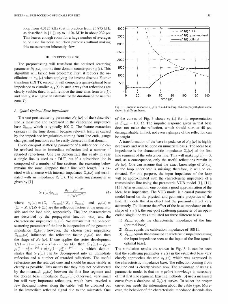
Fig. 3. Impulse response s11(t) of a 4-km-long, 0.4-mm polyethylene cableshown in different bases.

of the curves of Fig. 3 shows s11(t) for its representationin Zbase = 100 Ω. The impulse response given in that basedoes not make the reflection, which should start at 40 µs,distinguishable. In fact, not even a glimpse of the reflection canbe caught.

A transformation of the base impedance of S11(ω) is highlynecessary and will be done on numerical basis. The ideal baseimpedance is the characteristic impedance Zc(ω) of the firstline segment of the subscriber line. This will make ρg(ω) = 0,and, as a consequence, only the useful reflections remain inS11(ω). One can assume that the exact knowledge of Zc(ω)of the loop under test is missing; therefore, it will be es-timated. For this purpose, the input impedance of the loopwill be approximated with the characteristic impedance of atransmission line using the parametric VUB model [1], [14],[15]. After estimation, one obtains a good approximation of theideal base impedance. The VUB model is a causal parametricmodel based on the physical and geometric properties of theline. It models the skin effect and the proximity effect veryaccurately. To illustrate the effect of the base impedance on theshape of s11(t), the one-port scattering parameter of an open-ended single line was simulated for three different bases.

1) Zbase equals the characteristic impedance of the line(optimal base).

2) Zbase equals the calibration impedance of 100 Ω.3) Zbase equals the estimated characteristic impedance using

the input impedance seen at the input of the line (quasi-optimal base).

The simulation results are shown in Fig. 3. It can be seenthat the scattering parameter s11(t) in the estimated base veryclosely approaches the true s11(t), which was expressed inthe characteristic impedance base. The reflection coming fromthe line end is clearly visible now. The advantage of using aparametric model is that no a priori knowledge is necessaryof that first line segment. Existing methods [3] use a measuredcurve from a database of Zc(ω) curves. To select the propercurve, one needs the information about the cable type. More-over, the behavior of the characteristic impedance depends also

1512 IEEE TRANSACTIONS ON INSTRUMENTATION AND MEASUREMENT, VOL. 55, NO. 5, OCTOBER 2006

Fig. 4. Cross section of a two-wire line and the corresponding dimensions.

on external factors such as temperature and aging. Last but notleast, the properties of a twisted pair vary from pair to pair in thesame multipair cable due to the different twist rates used [16].Therefore, a model-based approach is more flexible to deal withthese unforeseen impedance deviations.

The characteristic impedance maximum likelihood estima-tor (15) uses the VUB physical line model. This estimatorwill identify the measured input impedance Zin(ω) of theone port with the characteristic impedance parametric modelZc,m(s,P). Because only four parameters control the shape ofthe characteristic impedance curve, the approximation of theinput impedance of the unknown DUT with such a “stiff” modelwill not be too liable to the impedance fluctuations, which areafter all present in Zin(ω) due to the reflections. The inputimpedance is given by

Zin(ω) =V1(ω)I1(ω)

. (5)

Using (1)–(3), the input impedance can be derived from themeasured scattering parameter S11(ω) defined in base Zbase asfollows:

Zin(ω) = Zbase(ω)1 + S11(ω)1 − S11(ω)

. (6)

The characteristic impedance model, in the case when thedielectric losses can be neglected, is given by

Zc,m(s,P) =

√θ4 + θ1

j√s

J0

J1+ θ1θ3

θ22

Ψ(s, θ2, θ3) (7)

where s = jω stands for the Laplace variable, P =(θ1, θ2, θ3, θ4)t represents the positive and real-valuedparameter vector, and Ji(x) is the Bessel function of order i(compact notation: Ji = Ji(θ3

√−s)). The proximity effectcontribution is described by

Ψ(s, θ2, θ3) =3θ22J3J2 + 2J1J2 + θ2J3J0

θ32J3J2 + θ2J1J2 + 3θ22J3J0 + J1J0. (8)

The model parameters can be derived from the physicalcable properties. Consider for this purpose a two-wire line asshown in Fig. 4 with the following properties for the metallicconductors: σc represents the conductivity, εc is the permittivity,µc stands for the permeability, and the circular wires with radiusa are separated from each other by distance D. The insulatormaterial is assumed to be lossless and can be characterized by

the permittivity εi and the permeability µi. The parameters canbe obtained as follows:

θ1 =1Cπa

õc

σc(9)

θ2 =( aD

)2

(10)

θ3 = a√µcσc (11)

θ4 =Lext

C(12)

with the per-unit-length external inductance given by

Lext =µi

πlnD

a(13)

and the per-unit-length capacitance can be easily obtained with

C =µiεiLext

. (14)

An output-error model was used, and the sample varianceσ2

S11of the measured S11(ω) was used and transformed into

the variance σ2Zin

of the input impedanceZin(ω) of the one port.The expression for the cost function CF can be easily found andis given by the following sum:

CF(P) =F∑

k=1

|Zin(k) − Zc,m(ωk,P)|2σ2

Zin(k)

(15)

where F is the number of frequency samples used. Solving theminimization problem

arg minP

CF(P) (16)

will be achieved by means of an iterative minimizer. TheLevenberg–Marquardt [17] method is chosen. It combinesthe Gauss–Newton and gradient-descent procedures. A start-ing value for P is obtained by calculating P for a plain0.5-mm polyethylene-insulated copper two-wire line withthe following parameters: a = 0.25 mm, D = 1 mm, σc =58.7 × 106 S/m, εc = ε0, µc = µ0, εi = 2.26ε0, µi = µ0, ε0 =(36π)−1 × 10−9 F/m, and µ0 = 4π × 10−7 H/m.

A measurement example based on a polyethylene-insulated0.4-mm twisted pair line of 3000 m long is shown in Fig. 5to demonstrate the technique. We remark that the same DUTis used to produce the subsequent graphs in the next sections.The line end is left open; thus, the closer the first significantreflection point is located to the CO injection point, the morethe input impedance of that loop, seen from the CO, will deviatefrom the characteristic impedance of the first line segment. As aresult, the modeling errors will increase. However, it was foundthat that the proposed technique is robust enough: This meansthat the found base impedance approaches the characteristicimpedance of the first line segment close enough, even with themodeling errors. In practice, the method could be applied on allkinds of subscriber line topologies, except when a bridged tapis located at or very near to the CO itself, which is practicallynonexistent.

BOETS et al.: PREPROCESSING OF SIGNALS FOR SELT 1513

Fig. 5. Measured input impedance Zin(ω) and the estimated characteristic impedance Zc,m(ω) for a 3-km-long, 0.4-mm cable. At low frequencies, the modeldeviates more from the measurement due to the reflections.

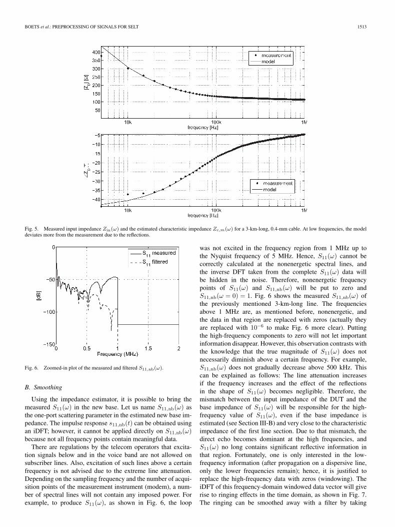
Fig. 6. Zoomed-in plot of the measured and filtered S11,nb(ω).

B. Smoothing

Using the impedance estimator, it is possible to bring themeasured S11(ω) in the new base. Let us name S11,nb(ω) asthe one-port scattering parameter in the estimated new base im-pedance. The impulse response s11,nb(t) can be obtained usingan iDFT; however, it cannot be applied directly on S11,nb(ω)because not all frequency points contain meaningful data.

There are regulations by the telecom operators that excita-tion signals below and in the voice band are not allowed onsubscriber lines. Also, excitation of such lines above a certainfrequency is not advised due to the extreme line attenuation.Depending on the sampling frequency and the number of acqui-sition points of the measurement instrument (modem), a num-ber of spectral lines will not contain any imposed power. Forexample, to produce S11(ω), as shown in Fig. 6, the loop

was not excited in the frequency region from 1 MHz up tothe Nyquist frequency of 5 MHz. Hence, S11(ω) cannot becorrectly calculated at the nonenergetic spectral lines, andthe inverse DFT taken from the complete S11(ω) data willbe hidden in the noise. Therefore, nonenergetic frequencypoints of S11(ω) and S11,nb(ω) will be put to zero andS11,nb(ω = 0) = 1. Fig. 6 shows the measured S11,nb(ω) ofthe previously mentioned 3-km-long line. The frequenciesabove 1 MHz are, as mentioned before, nonenergetic, andthe data in that region are replaced with zeros (actually theyare replaced with 10−6 to make Fig. 6 more clear). Puttingthe high-frequency components to zero will not let importantinformation disappear. However, this observation contrasts withthe knowledge that the true magnitude of S11(ω) does notnecessarily diminish above a certain frequency. For example,S11,nb(ω) does not gradually decrease above 500 kHz. Thiscan be explained as follows: The line attenuation increasesif the frequency increases and the effect of the reflectionsin the shape of S11(ω) becomes negligible. Therefore, themismatch between the input impedance of the DUT and thebase impedance of S11(ω) will be responsible for the high-frequency value of S11(ω), even if the base impedance isestimated (see Section III-B) and very close to the characteristicimpedance of the first line section. Due to that mismatch, thedirect echo becomes dominant at the high frequencies, andS11(ω) no long contains significant reflective information inthat region. Fortunately, one is only interested in the low-frequency information (after propagation on a dispersive line,only the lower frequencies remain); hence, it is justified toreplace the high-frequency data with zeros (windowing). TheiDFT of this frequency-domain windowed data vector will giverise to ringing effects in the time domain, as shown in Fig. 7.The ringing can be smoothed away with a filter by taking

1514 IEEE TRANSACTIONS ON INSTRUMENTATION AND MEASUREMENT, VOL. 55, NO. 5, OCTOBER 2006

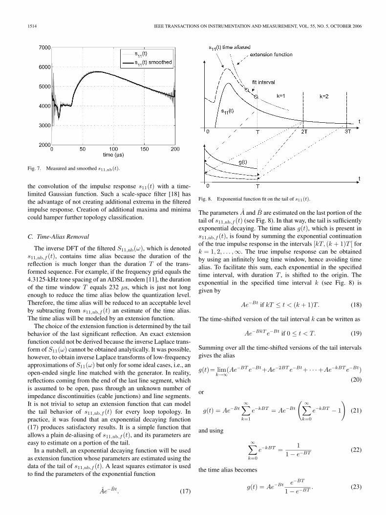
Fig. 7. Measured and smoothed s11,nb(t).

the convolution of the impulse response s11(t) with a time-limited Gaussian function. Such a scale-space filter [18] hasthe advantage of not creating additional extrema in the filteredimpulse response. Creation of additional maxima and minimacould hamper further topology classification.

C. Time-Alias Removal

The inverse DFT of the filtered S11,nb(ω), which is denoteds11,nb,f (t), contains time alias because the duration of thereflection is much longer than the duration T of the trans-formed sequence. For example, if the frequency grid equals the4.3125-kHz tone spacing of an ADSL modem [11], the durationof the time window T equals 232 µs, which is just not longenough to reduce the time alias below the quantization level.Therefore, the time alias will be reduced to an acceptable levelby subtracting from s11,nb,f (t) an estimate of the time alias.The time alias will be modeled by an extension function.

The choice of the extension function is determined by the tailbehavior of the last significant reflection. An exact extensionfunction could not be derived because the inverse Laplace trans-form of S11(ω) cannot be obtained analytically. It was possible,however, to obtain inverse Laplace transforms of low-frequencyapproximations of S11(ω) but only for some ideal cases, i.e., anopen-ended single line matched with the generator. In reality,reflections coming from the end of the last line segment, whichis assumed to be open, pass through an unknown number ofimpedance discontinuities (cable junctions) and line segments.It is not trivial to setup an extension function that can modelthe tail behavior of s11,nb,f (t) for every loop topology. Inpractice, it was found that an exponential decaying function(17) produces satisfactory results. It is a simple function thatallows a plain de-aliasing of s11,nb,f (t), and its parameters areeasy to estimate on a portion of the tail.

In a nutshell, an exponential decaying function will be usedas extension function whose parameters are estimated using thedata of the tail of s11,nb,f (t). A least squares estimator is usedto find the parameters of the exponential function

Ae−Bt. (17)

Fig. 8. Exponential function fit on the tail of s11(t).

The parameters A and B are estimated on the last portion of thetail of s11,nb,f (t) (see Fig. 8). In that way, the tail is sufficientlyexponential decaying. The time alias g(t), which is present ins11,nb,f (t), is found by summing the exponential continuationof the true impulse response in the intervals [kT, (k + 1)T [ fork = 1, 2, . . . ,∞. The true impulse response can be obtainedby using an infinitely long time window, hence avoiding timealias. To facilitate this sum, each exponential in the specifiedtime interval, with duration T , is shifted to the origin. Theexponential in the specified time interval k (see Fig. 8) isgiven by

Ae−Bt if kT ≤ t < (k + 1)T. (18)

The time-shifted version of the tail interval k can be written as

Ae−BkT e−Bt if 0 ≤ t < T. (19)

Summing over all the time-shifted versions of the tail intervalsgives the alias

g(t)= limk→∞

(Ae−BT e−Bt+Ae−2BT e−Bt+ · · · +Ae−kBT e−Bt)

(20)

or

g(t) = Ae−Bt∞∑

k=1

e−kBT = Ae−Bt

( ∞∑k=0

e−kBT − 1

)(21)

and using

∞∑k=0

e−kBT =1

1 − e−BT(22)

the time alias becomes

g(t) = Ae−Bt e−BT

1 − e−BT. (23)

BOETS et al.: PREPROCESSING OF SIGNALS FOR SELT 1515

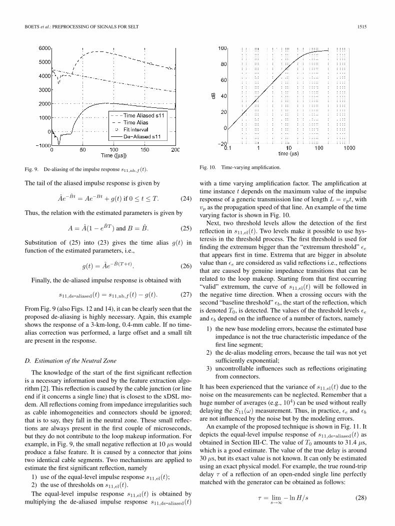
Fig. 9. De-aliasing of the impulse response s11,nb,f (t).

The tail of the aliased impulse response is given by

Ae−Bt = Ae−Bt + g(t) if 0 ≤ t ≤ T. (24)

Thus, the relation with the estimated parameters is given by

A = A(1 − eBT ) and B = B. (25)

Substitution of (25) into (23) gives the time alias g(t) infunction of the estimated parameters, i.e.,

g(t) = Ae−B(T+t). (26)

Finally, the de-aliased impulse response is obtained with

s11,de-aliased(t) = s11,nb,f (t) − g(t). (27)

From Fig. 9 (also Figs. 12 and 14), it can be clearly seen that theproposed de-aliasing is highly necessary. Again, this exampleshows the response of a 3-km-long, 0.4-mm cable. If no time-alias correction was performed, a large offset and a small tiltare present in the response.

D. Estimation of the Neutral Zone

The knowledge of the start of the first significant reflectionis a necessary information used by the feature extraction algo-rithm [2]. This reflection is caused by the cable junction (or lineend if it concerns a single line) that is closest to the xDSL mo-dem. All reflections coming from impedance irregularities suchas cable inhomogeneities and connectors should be ignored;that is to say, they fall in the neutral zone. These small reflec-tions are always present in the first couple of microseconds,but they do not contribute to the loop makeup information. Forexample, in Fig. 9, the small negative reflection at 10 µs wouldproduce a false feature. It is caused by a connector that joinstwo identical cable segments. Two mechanisms are applied toestimate the first significant reflection, namely

1) use of the equal-level impulse response s11,el(t);2) the use of thresholds on s11,el(t).The equal-level impulse response s11,el(t) is obtained by

multiplying the de-aliased impulse response s11,de-aliased(t)

Fig. 10. Time-varying amplification.

with a time varying amplification factor. The amplification attime instance t depends on the maximum value of the impulseresponse of a generic transmission line of length L = vpt, withvp as the propagation speed of that line. An example of the timevarying factor is shown in Fig. 10.

Next, two threshold levels allow the detection of the firstreflection in s11,el(t). Two levels make it possible to use hys-teresis in the threshold process. The first threshold is used forfinding the extremum bigger than the “extremum threshold” εethat appears first in time. Extrema that are bigger in absolutevalue than εe are considered as valid reflections i.e., reflectionsthat are caused by genuine impedance transitions that can berelated to the loop makeup. Starting from that first occurring“valid” extremum, the curve of s11,el(t) will be followed inthe negative time direction. When a crossing occurs with thesecond “baseline threshold” εb, the start of the reflection, whichis denoted T0, is detected. The values of the threshold levels εeand εb depend on the influence of a number of factors, namely

1) the new base modeling errors, because the estimated baseimpedance is not the true characteristic impedance of thefirst line segment;

2) the de-alias modeling errors, because the tail was not yetsufficiently exponential;

3) uncontrollable influences such as reflections originatingfrom connectors.

It has been experienced that the variance of s11,el(t) due to thenoise on the measurements can be neglected. Remember that ahuge number of averages (e.g., 104) can be used without reallydelaying the S11(ω) measurement. Thus, in practice, εe and εbare not influenced by the noise but by the modeling errors.

An example of the proposed technique is shown in Fig. 11. Itdepicts the equal-level impulse response of s11,de-aliased(t) asobtained in Section III-C. The value of T0 amounts to 31.4 µs,which is a good estimate. The value of the true delay is around30 µs, but its exact value is not known. It can only be estimatedusing an exact physical model. For example, the true round-tripdelay τ of a reflection of an open-ended single line perfectlymatched with the generator can be obtained as follows:

τ = lims→∞− lnH/s (28)

1516 IEEE TRANSACTIONS ON INSTRUMENTATION AND MEASUREMENT, VOL. 55, NO. 5, OCTOBER 2006

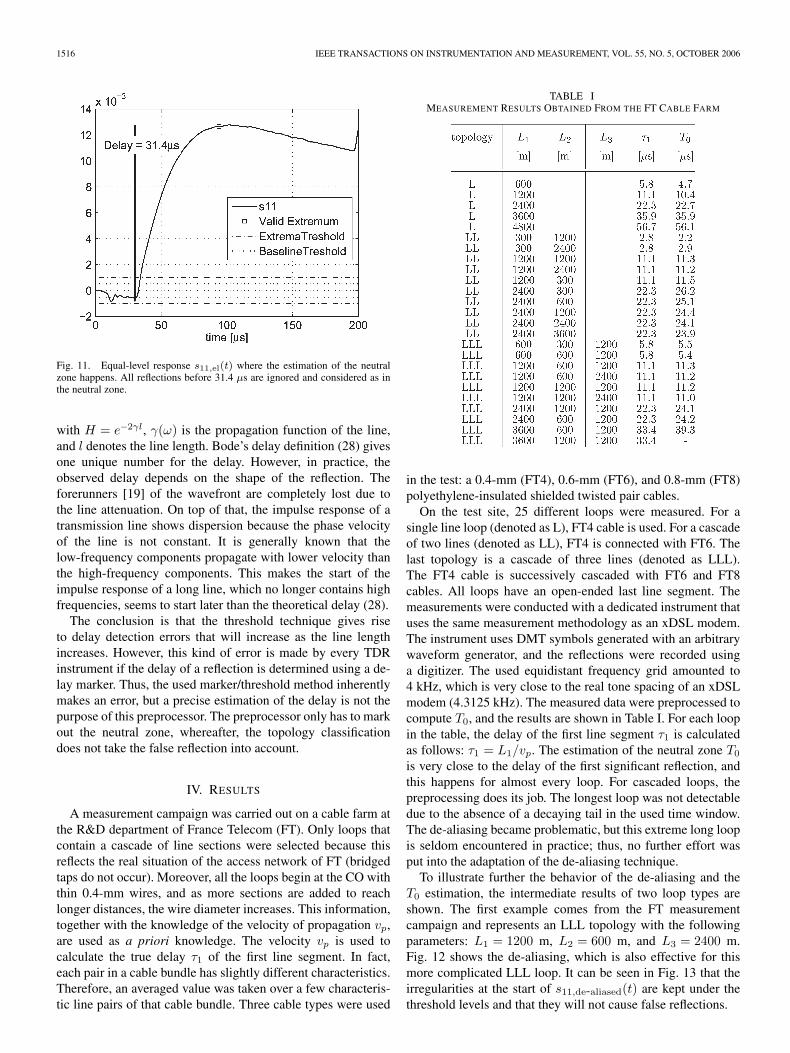
Fig. 11. Equal-level response s11,el(t) where the estimation of the neutralzone happens. All reflections before 31.4 µs are ignored and considered as inthe neutral zone.

with H = e−2γl, γ(ω) is the propagation function of the line,and l denotes the line length. Bode’s delay definition (28) givesone unique number for the delay. However, in practice, theobserved delay depends on the shape of the reflection. Theforerunners [19] of the wavefront are completely lost due tothe line attenuation. On top of that, the impulse response of atransmission line shows dispersion because the phase velocityof the line is not constant. It is generally known that thelow-frequency components propagate with lower velocity thanthe high-frequency components. This makes the start of theimpulse response of a long line, which no longer contains highfrequencies, seems to start later than the theoretical delay (28).

The conclusion is that the threshold technique gives riseto delay detection errors that will increase as the line lengthincreases. However, this kind of error is made by every TDRinstrument if the delay of a reflection is determined using a de-lay marker. Thus, the used marker/threshold method inherentlymakes an error, but a precise estimation of the delay is not thepurpose of this preprocessor. The preprocessor only has to markout the neutral zone, whereafter, the topology classificationdoes not take the false reflection into account.

IV. RESULTS

A measurement campaign was carried out on a cable farm atthe R&D department of France Telecom (FT). Only loops thatcontain a cascade of line sections were selected because thisreflects the real situation of the access network of FT (bridgedtaps do not occur). Moreover, all the loops begin at the CO withthin 0.4-mm wires, and as more sections are added to reachlonger distances, the wire diameter increases. This information,together with the knowledge of the velocity of propagation vp,are used as a priori knowledge. The velocity vp is used tocalculate the true delay τ1 of the first line segment. In fact,each pair in a cable bundle has slightly different characteristics.Therefore, an averaged value was taken over a few characteris-tic line pairs of that cable bundle. Three cable types were used

TABLE IMEASUREMENT RESULTS OBTAINED FROM THE FT CABLE FARM

in the test: a 0.4-mm (FT4), 0.6-mm (FT6), and 0.8-mm (FT8)polyethylene-insulated shielded twisted pair cables.

On the test site, 25 different loops were measured. For asingle line loop (denoted as L), FT4 cable is used. For a cascadeof two lines (denoted as LL), FT4 is connected with FT6. Thelast topology is a cascade of three lines (denoted as LLL).The FT4 cable is successively cascaded with FT6 and FT8cables. All loops have an open-ended last line segment. Themeasurements were conducted with a dedicated instrument thatuses the same measurement methodology as an xDSL modem.The instrument uses DMT symbols generated with an arbitrarywaveform generator, and the reflections were recorded usinga digitizer. The used equidistant frequency grid amounted to4 kHz, which is very close to the real tone spacing of an xDSLmodem (4.3125 kHz). The measured data were preprocessed tocompute T0, and the results are shown in Table I. For each loopin the table, the delay of the first line segment τ1 is calculatedas follows: τ1 = L1/vp. The estimation of the neutral zone T0

is very close to the delay of the first significant reflection, andthis happens for almost every loop. For cascaded loops, thepreprocessing does its job. The longest loop was not detectabledue to the absence of a decaying tail in the used time window.The de-aliasing became problematic, but this extreme long loopis seldom encountered in practice; thus, no further effort wasput into the adaptation of the de-aliasing technique.

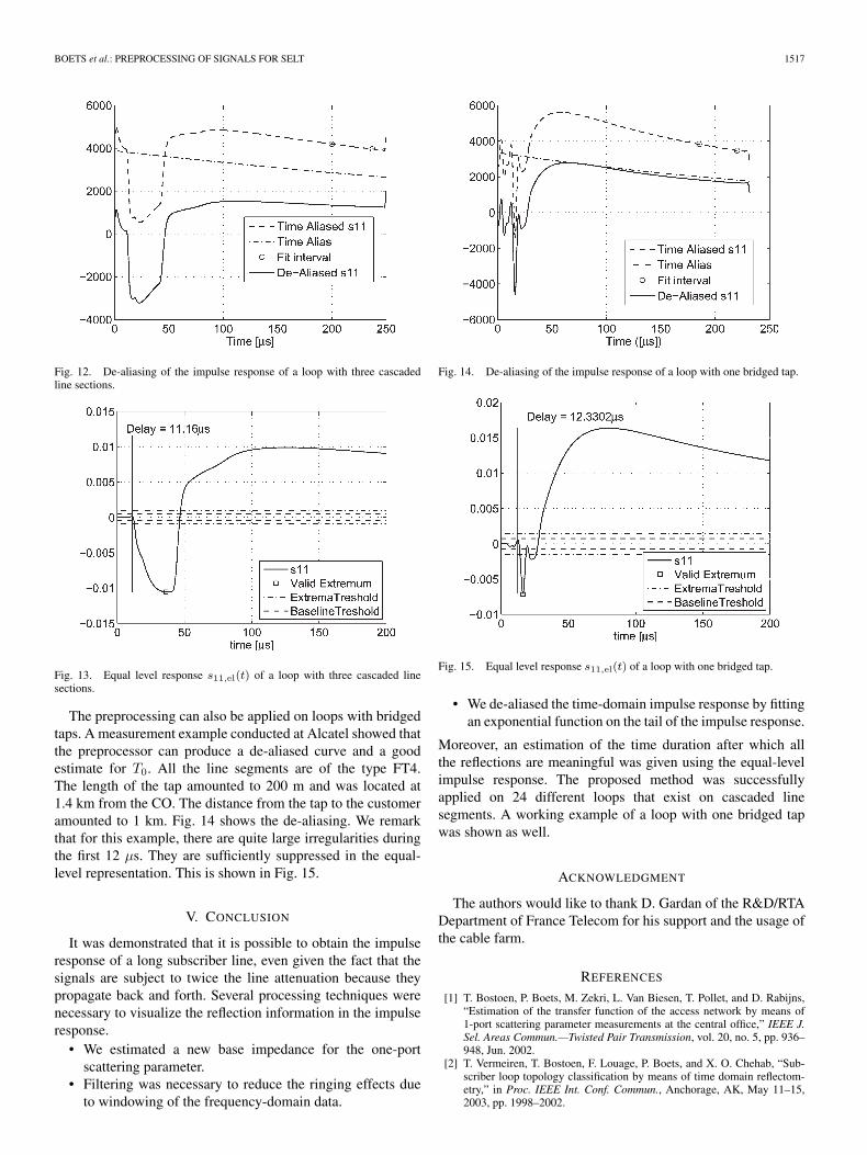
To illustrate further the behavior of the de-aliasing and theT0 estimation, the intermediate results of two loop types areshown. The first example comes from the FT measurementcampaign and represents an LLL topology with the followingparameters: L1 = 1200 m, L2 = 600 m, and L3 = 2400 m.Fig. 12 shows the de-aliasing, which is also effective for thismore complicated LLL loop. It can be seen in Fig. 13 that theirregularities at the start of s11,de-aliased(t) are kept under thethreshold levels and that they will not cause false reflections.

BOETS et al.: PREPROCESSING OF SIGNALS FOR SELT 1517

Fig. 12. De-aliasing of the impulse response of a loop with three cascadedline sections.

Fig. 13. Equal level response s11,el(t) of a loop with three cascaded linesections.

The preprocessing can also be applied on loops with bridgedtaps. A measurement example conducted at Alcatel showed thatthe preprocessor can produce a de-aliased curve and a goodestimate for T0. All the line segments are of the type FT4.The length of the tap amounted to 200 m and was located at1.4 km from the CO. The distance from the tap to the customeramounted to 1 km. Fig. 14 shows the de-aliasing. We remarkthat for this example, there are quite large irregularities duringthe first 12 µs. They are sufficiently suppressed in the equal-level representation. This is shown in Fig. 15.

V. CONCLUSION

It was demonstrated that it is possible to obtain the impulseresponse of a long subscriber line, even given the fact that thesignals are subject to twice the line attenuation because theypropagate back and forth. Several processing techniques werenecessary to visualize the reflection information in the impulseresponse.

• We estimated a new base impedance for the one-portscattering parameter.

• Filtering was necessary to reduce the ringing effects dueto windowing of the frequency-domain data.

Fig. 14. De-aliasing of the impulse response of a loop with one bridged tap.

Fig. 15. Equal level response s11,el(t) of a loop with one bridged tap.

• We de-aliased the time-domain impulse response by fittingan exponential function on the tail of the impulse response.

Moreover, an estimation of the time duration after which allthe reflections are meaningful was given using the equal-levelimpulse response. The proposed method was successfullyapplied on 24 different loops that exist on cascaded linesegments. A working example of a loop with one bridged tapwas shown as well.

ACKNOWLEDGMENT

The authors would like to thank D. Gardan of the R&D/RTADepartment of France Telecom for his support and the usage ofthe cable farm.

REFERENCES

[1] T. Bostoen, P. Boets, M. Zekri, L. Van Biesen, T. Pollet, and D. Rabijns,“Estimation of the transfer function of the access network by means of1-port scattering parameter measurements at the central office,” IEEE J.Sel. Areas Commun.—Twisted Pair Transmission, vol. 20, no. 5, pp. 936–948, Jun. 2002.

[2] T. Vermeiren, T. Bostoen, F. Louage, P. Boets, and X. O. Chehab, “Sub-scriber loop topology classification by means of time domain reflectom-etry,” in Proc. IEEE Int. Conf. Commun., Anchorage, AK, May 11–15,2003, pp. 1998–2002.

1518 IEEE TRANSACTIONS ON INSTRUMENTATION AND MEASUREMENT, VOL. 55, NO. 5, OCTOBER 2006

[3] S. Galli and D. L. Waring, “Loop makeup identification via singleended testing: Beyond mere loop qualification,” IEEE J. Sel. AreasCommun.—Twisted Pair Transmission, vol. 20, no. 5, pp. 923–935,Jun. 2002.

[4] S. Galli and K. J. Kerpez, “Single-ended loop make-up identifi-cation—Part I: A method of analyzing TDR measurements,” IEEE Trans.Instrum. Meas., vol. 55, no. 2, pp. 528–537, Apr. 2006.

[5] K. J. Kerpez and S. Galli, “Single-ended loop make-up identi-fication—Part II: Improved algorithms and performance results,” IEEETrans. Instrum. Meas., vol. 55, no. 2, pp. 538–549, Apr. 2006.

[6] K. J. Kerpez, D. L. Waring, S. Galli, J. Dixon, and P. Madon, “AdvancedDSL management,” IEEE Commun. Mag., vol. 41, no. 9, pp. 116–123,Sep. 2003.

[7] D. L. Waring, S. Galli, K. Kerpez, J. Lamb, and C. F. Valenti, “Analysistechniques for loop qualification and spectrum management,” in Proc.IWCS, Atlantic City, NJ, Nov. 13–16, 2000.

[8] W. Goralski, “xDSL loop qualification and testing,” IEEE Commun. Mag.,vol. 37, no. 5, pp. 79–83, May 1999.

[9] P. Boets, T. Bostoen, L. Van Biesen, and D. Gardan, “Single-endedline testing—A whitebox approach,” in Proc. 4th IASTED Int. Multi-Conf. Wireless Opt. Commun., Banff, AB, Canada, Jul. 8–10, 2004,pp. 393–398.

[10] S. Bregni and R. Melen, “Local loop unbundling in the Italian network,”IEEE Commun. Mag., vol. 40, no. 10, pp. 86–93, Oct. 2002.

[11] Asymmetric Digital Subscriber Line (ADSL) Metallic Interface, 1998.Issue 2. Available: ANSI T1.413.

[12] T. Bostoen, M. La Fauci, M. Luise, and P. Boets, “Disturber identificationfor single-ended line testing (SELT),” in Proc. IASTED Int. Conf. CIIT,Scottsdale, AZ, Nov. 17–19, 2003.

[13] S. Galli, C. Valenti, and K. Kerpez, “A frequency-domain approachto crosstalk identification in xDSL systems,” IEEE J. Sel. AreasCommun.—Special Issue on Multiuser Detection Techniques With Appli-cation to Wired and Wireless Communications Systems (Part I), vol. 19,no. 8, pp. 1497–1506, Aug. 2001.

[14] P. Boets, “Frequency identification of transmission lines from time do-main measurements,” Ph.D. dissertation, Free Univ. Brussels, Brussels,Belgium, Jun. 1997.

[15] P. Boets, M. Zekri, and L. Van Biesen, “On the identification of cables formetallic access networks,” in Proc. IEEE Instrum. Meas. Technol. Conf.,Budapest, Hungary, May 21–23, 2001, pp. 1348–1353.

[16] P. Boets, T. Bostoen, L. Van Biesen, and T. Pollet, “Measurement, cal-ibration and pre-processing of signals for single-ended subscriber lineidentification,” in Proc. IEEE Instrum. Meas. Technol. Conf., Vail, CO,May 20–22, 2003, pp. 338–343.

[17] R. Pintelon and J. Schoukens, System Identification, A Frequency DomainApproach. New York: IEEE Press, 2001.

[18] T. Lindberg, “Scale-space for discrete signals,” IEEE Trans. Pattern Anal.Mach. Intell., vol. 12, no. 3, pp. 234–254, Mar. 1990.

[19] A. Papoulis, The Fourier Integral and Its Applications. New York:McGraw-Hill, 1962.

Patrick Boets (M’99) was born in Duffel, Belgium,on January 8, 1963. He received the degree in civilengineering (electronics) and the Ph.D. degree fromthe Vrije Universiteit Brussel (VUB), Brussels, Bel-gium, in 1986 and 1997, respectively.

In 1987, he joined the Department of FundamentalElectricity and Instrumentation (ELEC), VUB, as anAssistant and later on as a Ph.D. Assistant. Currently,he is with Banama-Telecom, Brussels, Belgium: aspin-off company that designs and develops wirelesscommunication systems for rural areas. His major

interests are in the field of modeling of multiconductor transmission lines,data transmission, parameter estimation, computer-controlled measurementsystems, and terrestrial wireless communication. His current work is on single-ended line testing for xDSL systems and wireless communication systemdesign.

Tom Bostoen received the M.S. degree in physicalengineering from Ghent University, Ghent, Belgium,in 1998.

Since 1998, he has been with the Research Centerof Alcatel, Antwerp, Belgium. Currently, he is theProduct Manager of the 5530 Network Analyzer,Access Networks Division. In his previous function,he was the Project Manager of the digital subscriberline physical layer research project at the Researchand Innovation department. Before that, he studiedsingle-ended line testing as a Research Engineer in

the same department and contributed to International TelecommunicationsUnion (ITU) G.selt standardization.

Leo Van Biesen (M’90–SM’95) was born in Elsene,Belgium, on August 31, 1955. He received theelectromechanical engineer and the Ph.D. degreesfrom the Vrije Universiteit Brussel (VUB), Brussels,Belgium, in 1978 and 1983, respectively.

He is currently a Full Senior Professor withVUB. He teaches courses on fundamental electric-ity, electrical measurement techniques, signal theory,computer-controlled measurement systems, telecom-munication, underwater acoustics, and GeographicalInformation Systems for sustainable development of

environments. His current interests are signal theory, modern spectral esti-mators, time-domain reflectometry, wireless local loops, xDSL technologies,underwater acoustics, and expert systems for intelligent instrumentation.

Prof. Van Biesen is presiding over the International Measurement Confeder-ation (IMEKO) until September 2006. He is also a member of the board of theEuropean Telecommunication Engineers Federation (FITCE) Belgium and theInternational Scientific Radio Union (URSI) Belgium. He was the chairman ofIMEKO TC-7 from 1994 to 2000, the President Elect of IMEKO for the period2000–2003, and the Liaison Officer between the IEEE and IMEKO.

Thierry Pollet received the diploma degree in elec-trical engineering from the University of Ghent,Ghent, Belgium, in 1989.

In 1996, he joined the Alcatel Corporate ResearchCenter, Antwerp, Belgium. In 1999, he became theProject Manager within Research and Innovation,in charge of the research activities on metallic ac-cess, including topics such as asymmetric digitalsubscriber lines (ADSLs), very-high-data-rate DSL(VDSL), “all-digital loop,” and network characteri-zation. Currently, he is a distinguished member of

the technical staff for the Alcatel Technical Academy. His research interestsinclude solutions for end-to-end delivery of quality of service (QoS)-enabledInternet Protocol services on the scale of the Internet.

Mr. Pollet received the Alcatel Hi-Speed Award in 1999 for his contributionto the Alcatel patent portfolio in the DSL domain.