Preprint – Under peer review - arXiv

Prep

rin

t–

Un

der

peer

revi

ew

An installation-level model of China’s coal sector shows how its

decarbonization and energy security plans will reduce overseas coal

imports

Jorrit Gosens1,*, Alex Turnbull2, and Frank Jotzo1

1Crawford School of Public Policy, Australian National University, Acton, Australian Capital Territory, Australia

2Keshik Capital, Singapore*Corresponding author; [email protected]

Abstract

China aims for net-zero carbon emissions by 2060, and an emissions peak before 2030. This will reduceits consumption of coal for power generation and steel making. Simultaneously, China aims for improvedenergy security, primarily with expanded domestic coal production and transport infrastructure.

Here, we analyze effects of both these pressures on seaborne coal imports, with a purpose-built modelof China’s coal production, transport, and consumption system with installation-level geospatial andtechnical detail. This represents a 1000-fold increase in granularity versus earlier models, allowing repre-sentation of aspects that have previously been obscured.

We find that reduced Chinese coal consumption affects seaborne imports much more strongly thandomestic supply. Recent expansions of rail and port capacity, which reduce costs of getting domesticcoal to Southern coastal provinces, will further reduce demand for seaborne thermal coal and amplify theeffect of decarbonisation on coal imports. Seaborne coking coal imports are also likely to fall, because ofexpanded supply of cheap and high quality coking coal from neighbouring Mongolia.

Reducing the consumption of coal, used primarily in power generation and steelmaking, is a key elementof net-zero emissions plans or other long-term low-emissions strategies. This will affect the market outlookfor coal exporting countries, in particular as countries with domestic coal mining industries may seek tolimit negative effects on domestic coal mining industries [1]. China’s decarbonization plans are particularlyrelevant in this respect, as it is the world’s largest consumer of both thermal and coking coal, and a largesource of revenue for key exporters in the region, in particular Australia and Indonesia (Fig. 1).

Global coal markets have been the subject of much earlier research, and China has been a focal country inmost such studies given its dominant share in global coal production, consumption and imports. Yet, exactlyhow Chinese coal imports depend on domestic market and other developments remains poorly assessed.

In particular, such previous studies have typically used linear cost optimization with so-called multi-regional models, or node-and-link type models, to represent transport infrastructure. It’s important toaccurately account for transport in such analyses, given the large share of transport in the total cost of coal toconsumers, and because of the restrictions imposed by technical transport capacities of this infrastructure suchas railways and ports. However, previous work for such analyses has always used highly simplified networks,with even the most granular models using a few dozen nodes representing continents in global analysis,or provinces in China-focused analyses. These nodes conflate provincial-level production and demand intosingle points, and inter-provincial transport infrastructure into single links. This casts doubt on just howaccurately transport costs and capacity limits are really considered, and therefore how accurately the relativecompetitiveness of local and imported coal are assessed, in such models.

We drastically improve on this state of the art, with an installation-level model of China, that is, a modelthat represents every coal mine, power and steel plant, all ports, all railways with all stops, and an intercity

1

arX

iv:2

112.

0635

7v2

[ec

on.G

N]

14

Dec

202

1

Prep

rin

t–

Un

der

peer

revi

ew

Fig. 1: Global coal markets. Global consumption of thermal (a) and coking coal (b); global imports ofthermal (c) and coking coal (d); and revenue by destination for key exporters of coal (e-i; total of coking andthermal coal combined). Data source: (a-d): IEA[2], (e-i): UN Comtrade [3], panel (f) adjusted on the basisof Chinese customs data [4].

road network. Our model has 12,000 nodes and 40,000 links with accurate technical and geo-spatial detailfor individual installations. Calibration of this model versus real data for the year 2015-2019 shows its veryhigh accuracy, giving confidence about its predictions for future years.

We use this model to assess the sensitivity of levels of imported coal versus changes in Chinese consumptionof thermal and coking coal. We also consider different future scenarios as to where in China changes in coalconsumption would happen, and assess the likely effects of such geographic shifts in consumption on coalimports. Lastly, we consider different counterfactual scenarios, where we assess what import levels wouldhave been in the absence of recent infrastructural investments.

We find that overseas imports of thermal and coking coal coal are expected to fall between 52 and 96Mt by 2025 and between 56 and 124 Mt by 2030, from 209 Mt in 2019, depending on how rapidly, andwhere in China, decarbonization occurs. For coking coal, overseas imports are expected to fall between 9and 13 Mt by 2025 and between 12 and 17 Mt by 2030, from 68 Mt in 2019, getting pushed out mostlyby increased overland imports of cheap high quality coking coal from neighbouring Mongolia. If China hadnot made its recent substantial investments in its coal transport infrastructure, imports in 2025 and 2030would have remained at roughly similar levels to 2019 in high future demand scenarios, and would have fallensubstantially less in low future demand scenarios.

Factors determining China’s demand for coal imports

Although China imported only 7.2% of the thermal coal and 13.0% of the coking coal it consumed in 2019[2], it is the world’s largest importer by total volume (Fig. 1).

This Chinese reliance on imported coal cannot be explained by a limited domestic resource availability.Its total proved reserves stood at 141.6 Gt by the end of 2019, behind only the U.S., Russia, and Australia[5]. Whilst production capacity had a difficult time keeping in step with rapidly growing consumption inthe 2000’s, a growth of investment in coal mining capacity at 32% p.a. over 2000 to 2012 and slowingconsumption growth since then have largely balanced out again [6]. Currently, reserves of operational mineswere approximately 94.6 Gt, or about 24 years worth at 2019 consumption levels [7].

2

Prep

rin

t–

Un

der

peer

revi

ew

Fig. 2: Provincial-level coal supply balance in China. Supply balance as provincial level production- consumption. The full map on the left shows the route of the recently opened HaoJi railway. The cutouton the right shows major coal rail lines (black lines) and coal handling ports (blue dots). Consumption andproduction data source: SXcoal [4].

The geological conditions in China are also not such that production costs are exceptionally high [8].Chinese mines can produce 3,200 Mt of thermal coal per year, roughly the amount consumed in Chinaannually, at a mine-gate cost (that is, excluding transport) of $60/t or less; comparable to or below usualprices in global export markets [7].

There is geographical imbalance in Chinese coal production and consumption. China’s top 4 coal producers-Inner Mongolia, Shaanxi, Shanxi, and Xinjiang- produce about 79% of all domestic output. These are inland,Northern provinces, whilst coal consumption is concentrated in coastal provinces (Fig. 2). China has a numberof high capacity rail lines dedicated to the transport of coal, almost all of which start in these coal basinsand heads East towards the industrial heartland around Bohai Bay (Fig. 2), where China’s heavy industryincluding its steel making industry is concentrated. This is also where these rail lines connect with China’smajor coal ports, where coal is shipped South, in large part for electricity generation in coastal power plants.These coastal power plants have their own port facilities, which also allow international imports.

There is government regulation in almost every aspect of the coal sector, including mining permits,pricing, and limits on utilization of railways for coal, all of which impact competitiveness of foreign coals[9, 10]. Further, although never disclosed in official documents as far as we are aware, China is also consideredto use import quota, which are relaxed in times of temporary supply shortages [11].

China’s plans for emissions reductions and energy security

China is responsible for about 28% of global carbon dioxide emissions from energy [12], driven by its heavyreliance on coal for power generation (4,631 TWh or 53% of all global coal-fired power in 2020 [13]), and itsvery high steel output (1,053 Mt or 56% of global output in 2020 [14]).

However, China is also rapidly building out its renewable electricity generation capacity, with wind andsolar generating 9.5% of all power by 2020, up from 1.2% in 2010 [15]. Steel making, too, has become lesscarbon-intensive over time, due to increasing availability and use of steel scrap [16]. This replaces some ofthe demand for primary steel, made with iron ore and coking coal in conventional blast oxygen furnace steelmaking. Continued cost reductions of renewables and further growth in the availability of scrap in Chinacan be expected. China’s recently announced goal of net-zero carbon emission by 2060, with an interim goalof peak carbon emissions by 2030, are likely to further accelerate these decarbonization processes, although

3

Prep

rin

t–

Un

der

peer

revi

ew

the policies that will determine the emissions trajectory are still being designed [17]. The inevitably reducedconsumption of coal can be expected to affect coal imports.

In an effort to improve energy security and use more of the domestically mined coal, China has alsoinvested heavily in transport capacity. Between 2011 and 2020, over a period where total coal consumptionwas relatively stable (Fig. 1), the network length for freight rail lines used for the transport of coal grew fromcirca 36,000 to 46,600 km, with annual transport capacity of these lines growing from 1,788 Gt·km to 4,691Gt·km. This includes the 1,800 km HaoJi rail line, which started service in 2021. This line has a capacityof about 200 Mt per year, and is dedicated to the transport of coal, from the Ordos basin in Inner Mongoliato Central China’s inland provinces (Fig. 2). The handling capacity of the major coal ports in the North ofChina grew from 760 to 900 Mt per year over the same period [7, 18].

China is further expanding rail links into neighboring Mongolia, which is rapidly opening up miningcapacity for both thermal and high quality coking coals.

Lastly, China is building the largest ultra-high voltage (UHV) transmission network in the world. In somecases these UHV lines allow better use of the large hydropower, wind or solar PV bases in China’s West. Inother cases they transmit electricity from multi-GW coal-fired power plants in coal mining regions towardsdemand centers in the east, displacing some of the power generation in those coastal provinces, which importmost coal [19, 20].

Previous China coal supply models and assessments

A common approach in studies assessing international coal market developments is with multi-regional coalsupply models, which are linear optimization models that seek to satisfy a given level of demand for coalwhilst minimizing the total cost of production and transport of coal. At the core of such models are node& link networks that represent transport infrastructure between producing and consuming regions. Properrepresentations of transport infrastructure capacities and transport costs is key because of the significantshare of transport in total costs, and because of the large differences in costs of transport via truck, rail, orship.

Such multi-regional coal supply models have been used, for example, to investigate which coal-producingregions would optimally supply different consumers, in different scenarios of future growth or decline of globalcoal consumption, and/or what coal prices would be in different demand and supply scenarios [8, 19, 21, 22,23]. Both Haftendorn et al [8] and Paulus and Truby [19] forecast that rising Chinese consumption would leadto increases in Chinese imports exceeding 200 Mt between 2010 and 2030, under business as usual scenarios.Building on a more recent BAU scenario developed by the IEA, Auger et al [23] forecast a circa 27 Mt dropin Chinese imports, under essentially stable levels of consumption through 2030.

The same type of models have been used in a string of China-focused analyses. A number of these analysesfocused on substitution between different types of energy, and concluded there will be strong downwardpressure on coal demand and prices from competition with renewables or other fuels, though with littleexplicit assessment on volumes of coal imported [24, 25, 26]. Rioux et al [18] calculated that most of China’sgovernment plans for investments in rail and port infrastructure in the early 2010s would have highly positiveeconomic benefits. They estimated that bottle-necks in the coal transport system increased total systemsupply costs by circa $35 billion, largely because the high transport costs made domestic coals uncompetitiveversus imported coals, in particular for consumers in China’s Southern coastal provinces. A similar analysisfocused on the potential expansion of UHV transmission found that this could lead to $149 billion in netwelfare gains by 2030 [19]. Both papers estimated that the planned infrastructure investments might crowdout imports of coal entirely [18, 19]. Other analyses assessed China’s policies for cutting over-capacity coalmining from 2016 onwards, which were a bid to tackle falling profitability in the coal mining sector. The policywas found to be so effective that prices rose almost 50%, strongly increasing competitiveness of importedcoal [9, 6, 27].

Whilst these analyses have provided valuable insights into different and specific aspects of the economics ofthe global or Chinese coal supply system, their utility in answering how Chinese imports depend on domesticproduction capacity, transport capacities, and consumption levels, may still be limited, due to the limitedgeo-spatial detail in constructing these multi-regional models. Specifically, the regions, or nodes, in thesemodels typically aggregate large geographic areas, with China represented as about 5 or 6 regional nodes

4

Prep

rin

t–

Un

der

peer

revi

ew

in global models, whilst even the most granular models described above use Chinese provinces as individualnodes.

Such nodes aggregate all supply and demand for coal, as well as all port loading capacity within theprovince(s) they cover, whilst links between nodes aggregate all rail capacity and road connections betweenthem. This effectively gives the appearance that each consumer within the province(s) is equally well con-nected to all transport networks. The reality, as also identified in a plant-by-plant review of satellite imagesfor this research (see Methods), is that a large share of steel and power plants are directly on the coast oralong rivers, and have port facilities but not railway connections. They are therefore very poorly connectedto the landborne market, and almost entirely dependent on seaborne supplies, whether imported or shippedfrom northern ports.

A related aspect is the recognition that so many of these plants along the ocean or rivers have their ownport facilities for ocean-going vessels or river barges. None of the papers referred to above specifies whatvalues were used for port capacities of different nodes, so we cannot determine if these were included or not.However, none of them mentions specifically these port facilities at power and steel plants, and some refer tocapacities for ‘major’ or ‘main’ ports only [18, 9, 10]. These are highly relevant to the seaborne market: inJiangsu, the largest consumer of coal along the southern coast, total port capacity in 2020 was 593 Mt/yr,of which 273 Mt/yr located at power or steel plants with their own port facilities, in Guangdong, the secondlargest southern consumer, it was 137 Mt out of a total of 407 Mt of annual unloading capacity.

Lastly, the aggregation of railways between a limited number of nodes creates the false impression thate.g., all East-West bound lines are perfectly interconnected with all North-South lines, and that all rail lineswithin a certain area are connected with all port capacity in the same area. This aggregation may have beena sensible simplification in earlier research, but with the current availability of (open source) information onpower plants, steel plants, and railway networks, it is not a necessary simplification anymore.

An installation-level model of China’s coal market

Here, we introduce a multi-regional model of China’s coal production, transportation, and consumptionsystem, with installation-level geospatial and technical detail. The ‘XX China Coal model’, or ‘XX-CCM’(name censored for blind review), includes a network with tens of thousands of nodes and links (Table1); roughly a thousand-fold improvement in granularity versus the current the state of the art, allowingrepresentation of aspects that have been obscured in earlier models.

Each individual coal-fired power plant unit and steel plant is represented as a separate demand node.For each of these plants we have precise location, as well as technical characteristics such as generation orproduction capacity, and approximate conversion efficiency.

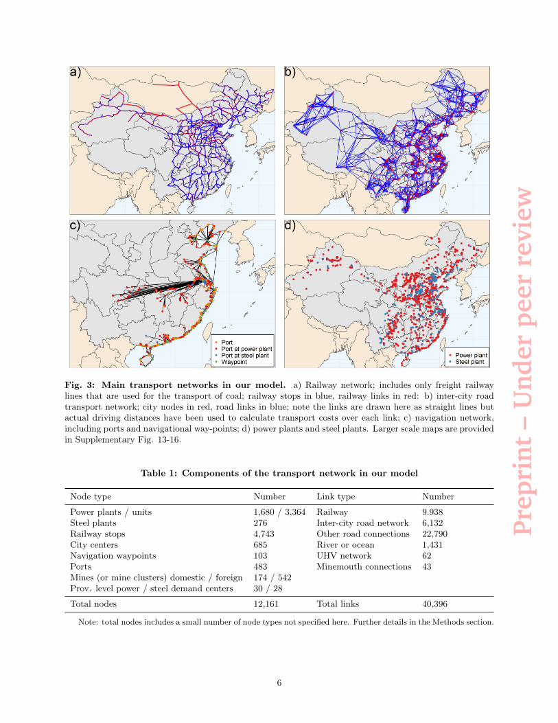
The model also includes a highly granular representation of China’s coal transport networks. First, itincludes a rail network, with route, distances between railway stops, and transport capacity of 145 freight raillines. Second, a road network with links between all of China’s 685 cities, and between other relevant typesof nodes, with actual driving distances determined for each link. Third, a navigation network with preciselocation and handling capacity for 483 individual ports, including port facilities at coastal steel and powerplants. Fourth, a representation of China’s rapidly expanding Ultra-High Voltage (UHV) network for thelong-distance transmission of electricity. The network includes accurate interconnections between differentrail lines, connections to the rail network for coastal power plants and all steel plants, and mine-mouthoperations (direct connections between mines and power plants) in key coal-bearing areas. An overviewof node and link types is provided in (Table 1), with illustrative maps of the key transport networks andlocations of power and steel plants in Fig. 3.

This network is the main component in a linear optimization model that minimizes total production andtransport costs, at exogenously determined levels of demand for thermal and coking coal.

5

Prep

rin

t–

Un

der

peer

revi

ew

Fig. 3: Main transport networks in our model. a) Railway network; includes only freight railwaylines that are used for the transport of coal; railway stops in blue, railway links in red: b) inter-city roadtransport network; city nodes in red, road links in blue; note the links are drawn here as straight lines butactual driving distances have been used to calculate transport costs over each link; c) navigation network,including ports and navigational way-points; d) power plants and steel plants. Larger scale maps are providedin Supplementary Fig. 13-16.

Table 1: Components of the transport network in our model

Node type Number Link type Number

Power plants / units 1,680 / 3,364 Railway 9.938Steel plants 276 Inter-city road network 6,132Railway stops 4,743 Other road connections 22,790City centers 685 River or ocean 1,431Navigation waypoints 103 UHV network 62Ports 483 Minemouth connections 43Mines (or mine clusters) domestic / foreign 174 / 542Prov. level power / steel demand centers 30 / 28

Total nodes 12,161 Total links 40,396

Note: total nodes includes a small number of node types not specified here. Further details in the Methods section.

6

Prep

rin

t–

Un

der

peer

revi

ew

Sensitivity of Chinese coal imports to consumption levels

We use our model to determine which mines, domestic or foreign, would supply thermal and coking coal,at various levels of Chinese demand. We purposely use a very wide range of future growth or reductionof consumption, in order to gauge the relationship between Chinese coal consumption levels and importedvolumes of coal.

The baseline model setting includes all transport infrastructure that is either operational or well underconstruction, and distributes the given future consumption of thermal and coking coal within China on thebasis of historical patterns (more details the Methods section).

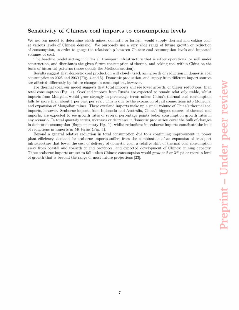
Results suggest that domestic coal production will closely track any growth or reduction in domestic coalconsumption to 2025 and 2030 (Fig. 4 and 5). Domestic production, and supply from different import sourcesare affected differently by future changes in consumption, however.

For thermal coal, our model suggests that total imports will see lower growth, or bigger reductions, thantotal consumption (Fig. 4). Overland imports from Russia are expected to remain relatively stable, whilstimports from Mongolia would grow strongly in percentage terms unless China’s thermal coal consumptionfalls by more than about 1 per cent per year. This is due to the expansion of rail connections into Mongolia,and expansion of Mongolian mines. These overland imports make up a small volume of China’s thermal coalimports, however. Seaborne imports from Indonesia and Australia, China’s biggest sources of thermal coalimports, are expected to see growth rates of several percentage points below consumption growth rates inany scenario. In total quantity terms, increases or decreases in domestic production cover the bulk of changesin domestic consumption (Supplementary Fig. 1), whilst reductions in seaborne imports constitute the bulkof reductions in imports in Mt terms (Fig. 4).

Beyond a general relative reduction in total consumption due to a continuing improvement in powerplant efficiency, demand for seaborne imports suffers from the combination of an expansion of transportinfrastructure that lower the cost of delivery of domestic coal, a relative shift of thermal coal consumptionaway from coastal and towards inland provinces, and expected development of Chinese mining capacity.These seaborne imports are set to fall unless Chinese consumption would grow at 2 or 3% pa or more; a levelof growth that is beyond the range of most future projections [23].

7

Prep

rin

t–

Un

der

peer

revi

ew

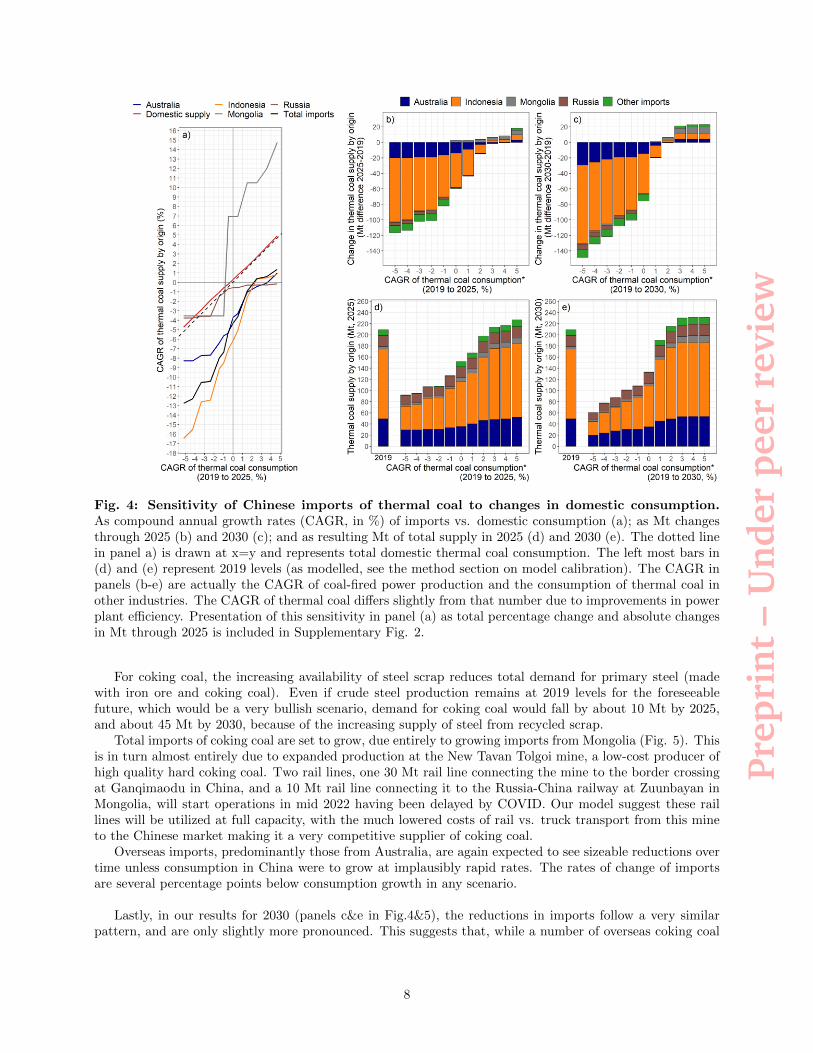
Fig. 4: Sensitivity of Chinese imports of thermal coal to changes in domestic consumption.As compound annual growth rates (CAGR, in %) of imports vs. domestic consumption (a); as Mt changesthrough 2025 (b) and 2030 (c); and as resulting Mt of total supply in 2025 (d) and 2030 (e). The dotted linein panel a) is drawn at x=y and represents total domestic thermal coal consumption. The left most bars in(d) and (e) represent 2019 levels (as modelled, see the method section on model calibration). The CAGR inpanels (b-e) are actually the CAGR of coal-fired power production and the consumption of thermal coal inother industries. The CAGR of thermal coal differs slightly from that number due to improvements in powerplant efficiency. Presentation of this sensitivity in panel (a) as total percentage change and absolute changesin Mt through 2025 is included in Supplementary Fig. 2.

For coking coal, the increasing availability of steel scrap reduces total demand for primary steel (madewith iron ore and coking coal). Even if crude steel production remains at 2019 levels for the foreseeablefuture, which would be a very bullish scenario, demand for coking coal would fall by about 10 Mt by 2025,and about 45 Mt by 2030, because of the increasing supply of steel from recycled scrap.

Total imports of coking coal are set to grow, due entirely to growing imports from Mongolia (Fig. 5). Thisis in turn almost entirely due to expanded production at the New Tavan Tolgoi mine, a low-cost producer ofhigh quality hard coking coal. Two rail lines, one 30 Mt rail line connecting the mine to the border crossingat Ganqimaodu in China, and a 10 Mt rail line connecting it to the Russia-China railway at Zuunbayan inMongolia, will start operations in mid 2022 having been delayed by COVID. Our model suggest these raillines will be utilized at full capacity, with the much lowered costs of rail vs. truck transport from this mineto the Chinese market making it a very competitive supplier of coking coal.

Overseas imports, predominantly those from Australia, are again expected to see sizeable reductions overtime unless consumption in China were to grow at implausibly rapid rates. The rates of change of importsare several percentage points below consumption growth in any scenario.

Lastly, in our results for 2030 (panels c&e in Fig.4&5), the reductions in imports follow a very similarpattern, and are only slightly more pronounced. This suggests that, while a number of overseas coking coal

8

Prep

rin

t–

Un

der

peer

revi

ew

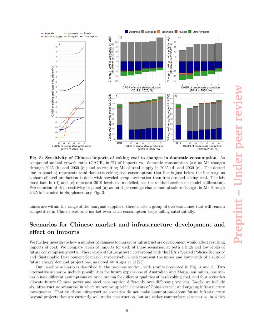
Fig. 5: Sensitivity of Chinese imports of coking coal to changes in domestic consumption. Ascompound annual growth rates (CAGR, in %) of imports vs. domestic consumption (a); as Mt changesthrough 2025 (b) and 2030 (c); and as resulting Mt of total supply in 2025 (d) and 2030 (e). The dottedline in panel a) represents total domestic coking coal consumption; that line is just below the line x=y, asa share of steel production is done with recycled scrap steel rather than iron ore and coking coal. The leftmost bars in (d) and (e) represent 2019 levels (as modelled, see the method section on model calibration).Presentation of this sensitivity in panel (a) as total percentage change and absolute changes in Mt through2025 is included in Supplementary Fig. 3.

mines are within the range of the marginal suppliers, there is also a group of overseas mines that will remaincompetitive in China’s seaborne market even when consumption keeps falling substantially.

Scenarios for Chinese market and infrastructure development andeffect on imports

We further investigate how a number of changes to market or infrastructure development would affect resultingimports of coal. We compare levels of imports for each of these scenarios, at both a high and low levels offuture consumption growth. These levels of future growth correspond with the IEA’s ‘Stated Policies Scenario’and ‘Sustainable Development Scenario’, respectively, which represent the upper and lower ends of a suite offuture energy demand projections, as noted by Auger et al [23].

Our baseline scenario is described in the previous section, with results presented in Fig. 4 and 5. Twoalternative scenarios include possibilities for future expansions of Australian and Mongolian mines, one sce-nario uses different assumptions on price premia for different qualities of hard coking coal, and four scenariosallocate future Chinese power and steel consumption differently over different provinces. Lastly, we includesix infrastructure scenarios, in which we remove specific elements of China’s recent and ongoing infrastructureinvestments. That is: these infrastructure scenarios do not make assumptions about future infrastructurebeyond projects that are currently well under construction, but are rather counterfactual scenarios, in which

9

Prep

rin

t–

Un

der

peer

revi

ew

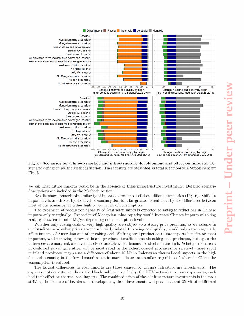
Fig. 6: Scenarios for Chinese market and infrastructure development and effect on imports. Forscenario definition see the Methods section. These results are presented as total Mt imports in SupplementaryFig. 5

we ask what future imports would be in the absence of these infrastructure investments. Detailed scenariodescriptions are included in the Methods section.

Results shows remarkable similarity of imports across most of these different scenarios (Fig. 6). Shifts inimport levels are driven by the level of consumption to a far greater extent than by the differences betweenmost of our scenarios, at either high or low levels of consumption.

The expansion of production capacity of Australian mines is expected to mitigate reductions in Chineseimports only marginally. Expansion of Mongolian mine capacity would increase Chinese imports of cokingcoal, by between 2 and 6 Mt/yr, depending on consumption levels.

Whether only coking coals of very high quality are subject to a strong price premium, as we assume inour baseline, or whether prices are more linearly related to coking coal quality, would only very marginallyaffect imports of Australian and other coking coal. Shifting steel production to major ports benefits overseasimporters, whilst moving it toward inland provinces benefits domestic coking coal producers, but again thedifferences are marginal, and even barely noticeable when demand for steel remains high. Whether reductionsin coal-fired power generation will be most rapid in the richer, coastal provinces, or relatively more rapidin inland provinces, may cause a difference of about 10 Mt in Indonesian thermal coal imports in the highdemand scenario; in the low demand scenario market losses are similar regardless of where in China theconsumption is reduced.

The largest differences to coal imports are those caused by China’s infrastructure investments. Theexpansion of domestic rail lines, the HaoJi rial line specifically, the UHV networks, or port expansions, eachhad their effect on thermal coal imports. The combined effect of these infrastructure investments is the moststriking. In the case of low demand development, these investments will prevent about 25 Mt of additional

10

Prep

rin

t–

Un

der

peer

revi

ew

imports. In the high demand scenarios, overseas imports would still be very similar to 2019 levels in 2025,had the Chinese government not invested in coal transport infrastructure.

For coking coal imports, these infrastructure investments have much more limited effects, apart from theexpanded rail capacity into Mongolia. Those rail lines enable an increase of approximately 15 Mt of imports.Our model also suggests that even if the rail lines to the New Tavan Tolgoi mine had not been built, cokingcoal imports would increase by about 6 Mt from 2019 levels by 2025. We should note, however, that ourmodel does not impose technical limits on the volume of coal that can be trucked across the border. Forimport of Australian coking coal, there is a difference of about 2 Mt between the most limited and mostexpansive infrastructure investments scenarios.

Results for 2030 are similar though more pronounced, in particular for reductions in thermal coal imports(Supplementary Fig. 4&6).

Conclusion and discussion

China has grown to be the world’s largest consumer and importer of thermal and coking coal. Its recent andfuture plans for energy security and decarbonization have, and will continue to, affect the consumption ofseaborne imports of coal in particular.

Using a new model that has far greater geo-spatial and technical detail than comparable models, har-nessing a wide range of data sources China’s, we have assessed scenarios for China’s future coal imports.Results show that Chinese imports of overseas coal are likely to fall substantially, in particular imports ofIndonesian thermal coal, and Australian thermal and coking coal, even under moderate reduction in Chinesecoal consumption. Accelerated decarbonisation, as well as recent infrastructure investments, and expansionof mine capacity in Mongolia, will amplify this trend.

Seaborne imports of thermal coal are expected to fall between 52 and 96 Mt by 2025 and between 56and 124 Mt by 2030, depending on how rapidly, and where in China, decarbonization occurs. For cokingcoal, seaborne imports are expected to fall between 9 and 13 Mt by 2025 and between 12 and 17 Mt by2030, whilst overland imports of coking coal from neighbouring Mongolia are expected to surge by circa 20Mt by 2025, and remain at roughly that level through 2030. The key factor is China’s recently completedor committed domestic coal transport infrastructure. If China had not substantially invested in its coaltransport infrastructure, imports in 2025 and 2030 would have remained at roughly similar levels to 2019 inhigh future demand scenarios, and would have fallen substantially less in low future demand scenarios.

This has clear implications for exporters in the Asian seaborne coal market, primarily thermal coal minesin Indonesia and thermal and coking coal mines in Australia. The expected drop in Chinese demand forseaborne imports in even the highest of future growth projections, should be considered in determining thefuture value of existing and planned mines, and in the predicted future revenue from coal export royaltiesand taxes flowing into government budgets for key exporting countries in the region.

The model presented here solves for optimal, i.e., lowest total cost of production and transport, as is usualfor these types of model. It does not consider factors such as politically imposed limits on imports from allor from certain countries, such as a recent halt on coal imports from Australia. Including such considerationswould require expanding the model to include representation of other key customers in the Asian coal market,including Japan, South Korea, India and Vietnam.

Our baseline scenario does not include any additional infrastructure development beyond projects thatare well under construction. Whilst it may be possible that further investment in rail lines to low-cost coalproducing regions in China’s West would push out more overseas suppliers, it is also likely that China hasreached ’peak coal infrastructure’, and that government planners won’t see great benefits from developingfurther big rail projects in a time of declining overall consumption.

Lastly, our model finds cost optimal supply for annual levels of demand, with restrictions in annualtransport capacities, again as is usual for these types of model. This does not very well account for temporaryand local demand peaks, caused for example by the seasonality of electricity demand and volatility of China’shydropower output, or for temporary supply disruptions such as caused by mine flooding or COVID-19 relatedproduction or transport restrictions. Whilst Chinese economic planners are demanding increased inventorystockpiles at power plants and key coal logistics hubs, in response to recent supply shortages leading to

11

Prep

rin

t–

Un

der

peer

revi

ew

rationing of power supply in a number of Southern provinces, such temporary spikes in supply shortages maymitigate the effects of some of the demand reductions on China’s coal imports predicted here.

12

Prep

rin

t–

Un

der

peer

revi

ew

Methods

Model description

Our model is a linear optimization problem for coal supply to the Chinese coal market, with an objectivefunction that minimizes the sum of production (mining) and transportation costs. The model includesseparate demand levels for electricity from coal-fired power, thermal coal use in other industries, and cokingcoal use in steel making. This demand is inelastic and must be met. It includes technical constraints on thecapacity of coal-fired power plants and steel plants, railway lines, and ports, and considers the conversionefficiency of coal-fired power plants. Model inputs on coal mining capacity, infrastructure development, andfuture demand taken from projections exogenous to the model (more below). The model solves for individualyears; for the results for 2025 and 2030 we do account for mine depletion by cross-checking that all minesproducing in 2025 or 2030 had six or eleven years worth of modelled production levels in them in the year2019. The mathematical formulation of the model is provided at the end of this section.

The system of supply, transport and consumption in the model is represented as a node & link model.The key contribution of our model is the strongly improved granularity of the coal transport network that webuild; individual components of this network and how they are strung together are described below (section‘network construction and data collection’).

All links in the model are transport links for physical amounts of coal, with constraints defined in Mt,whilst demand for coal-fired power and other thermal coal use is defined in PJ. Different thermal coals aregrouped in calorific value bins, with steps of 250 kcal/kg.

Demand for coal-fired power is placed in provincial-level electricity demand nodes, and can be satisfiedby power plant units within the province, or by power transmitted over the inter-provincial UHV network.

Demand for thermal coal for other purposes is determined as PJ of primary energy, and is placed atcity-center nodes.

Demand for steel is placed in provincial level steel demand nodes and is defined in Mt of crude, primarysteel. We consider a mix of hard coking coal (HCC), semi-soft coal (SCC), and pulverized coal for injection(PCI), needed to produce a tonne of steel, with the same mix used by all steel plants. Only steel plant nodesare connected with these steel demand nodes.

Our model is written in Python, with linear problem formulation done using the package PuLP (pypi.org/project/PuLP). This allows for replication or development with fully free and open source software.The size of the network in our model does mean it requires fairly substantial computing resources. We use acommercial cloud computing service to process input data on demand levels and model constraints to createa problem definition (.lp) file. For our model, this process requires about 10 hours on an instance with 72virtual CPU and 144 Gb of RAM. We then download the lp file and solve locally using the CPLEX solvervia IBM’s CPLEX Interactive. Either step can also be done locally in Python, albeit considerably slower;scripts for both alternative routes are included in our public data and code repository.

Mathematical formulation of the model

The sets, parameters, and variables included in the model are listed in tables 2 to 4.The objective function eq. (1) minimizes the total production and transport of coal, plus the cost of

transmission of electricity via the inter-provincial UHV network. The cost of transport over each link is madeup of a fixed handling cost, plus a variable distance based component. The variable transport cost variesby transport mode, whilst the handling charges vary with switches between different transport modes (e.g.,from mine to truck or from mine to rail). Transmission costs over the UHV network are pre-calculated, andare based on the distance of the transmission link. We apply a conversion efficiency factor to each UHV linkto represent line losses, which are based on line length and type of UHV connection (DC or AC).

The model includes the following constraints. Firstly, a supply constraint eq. (2) that limits the supplyof any type of coal by any node to below or equal to the production capacity for that type of coal.

The mass balance eq. (3) states that the supply plus transport flows into a node, must be at least equalto the transport flow out of that node, for each type of coal. The energy balance eq. (4) states that the totalenergy content of the supply plus transport flows into a node, must be at least equal to the energy demandfor electricity generation, plus the energy demand for thermal coal for other purposes, plus the total energycontent of the transport flows out of that node.

13

Prep

rin

t–

Un

der

peer

revi

ew

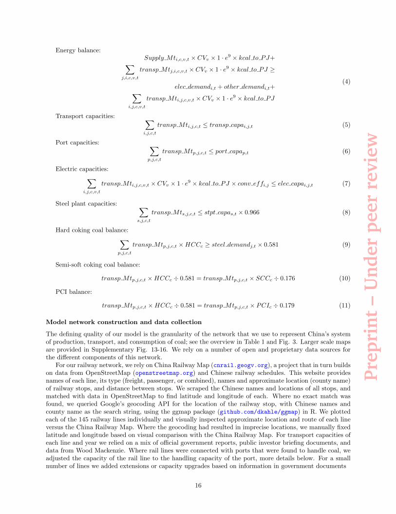
The transport capacity constraint eq. (5) limits the total volume of coal transported over each link to itstransport capacity; eq. (6) constrains volumes flowing out of port nodes to port handling capacity.

We represent conversion losses in power generation by multiplying the the energy content of the differenttypes of coal arriving in power plant unit nodes with the power plant unit’s conversion efficiency. Theelectrical generation capacity of these power plant units is represented in eq. (7) by imposing a transmissioncapacity on links between power plant units and provincial-level electricity demand nodes, which is equal tothe total energy content of the coal, multiplied by the conversion efficiency of the power plant unit; the samelogic is applied to links in the UHV network.

We represent the process of steel making by requiring the links between steel plants and steel demandcenters to transport a volume of coking coal required for the production of the demanded volume of steel.eq. (8) limits the flow of coking coal over these links to the amount of coking required for the steel plant torun at full production capacity. The hard coking coal balance eq. (9) states that all steel demand must besatisfied, and simultaneously that this should be done with the required 581 kg of HCC for every ton of steelproduced. eqs. (10) and (11) dictate that the required mix of coking coals, with 581 kg of HCC, 176 kg ofSCC, and 179 kg PCI, is used.

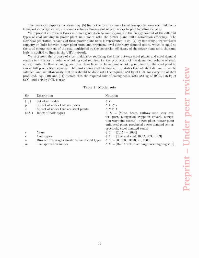
Table 2: Model sets

Set Description Notation

(i,j ) Set of all nodes ∈ Ip Subset of nodes that are ports ∈ P ⊂ Is Subset of nodes that are steel plants ∈ S ⊂ I(k,k’ ) Index of node types ∈ K = [Mine, basin, railway stop, city cen-

ter, port, navigation waypoint (river), naviga-tion waypoint (ocean), power plant, power plantunit, steel plant, provincial power demand center,provincial steel demand center]

t Years ∈ T = [2015,· · · ,2030]c Coal types ∈ C = [Thermal coal, HCC, SCC, PCI]v Bins with average calorific value of coal types ∈ V = [0, 3000, 3250,· · · , 7000]m Transportation modes ∈M = [Rail, truck, river barge, ocean-going ship]

14

Prep

rin

t–

Un

der

peer

revi

ew

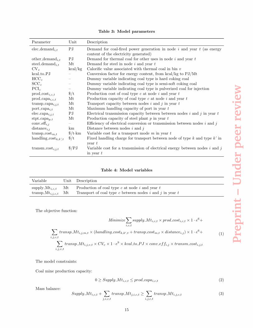
Table 3: Model parameters

Parameter Unit Description

elec demandi,t PJ Demand for coal-fired power generation in node i and year t (as energycontent of the electricity generated)

other demandi,t PJ Demand for thermal coal for other uses in node i and year tsteel demandi,t Mt Demand for steel in node i and year tCVv kcal/kg Calorific value associated with thermal coal in bin vkcal to PJ – Conversion factor for energy content, from kcal/kg to PJ/MtHCCc – Dummy variable indicating coal type is hard coking coalSCCc – Dummy variable indicating coal type is semi-soft coking coalPCIc – Dummy variable indicating coal type is pulverized coal for injectionprod costi,c,t $/t Production cost of coal type c at node i and year tprod capai,c,t Mt Production capacity of coal type c at node i and year ttransp capai,j,t Mt Transport capacity between nodes i and j in year tport capai,t Mt Maximum handling capacity of port in year telec capai,j,t PJ Electrical transmission capacity between between nodes i and j in year tstpt capap,t Mt Production capacity of steel plant p in year tconv effi,j – Efficiency of electrical conversion or transmission between nodes i and jdistancei,j km Distance between nodes i and jtransp costm,t $/t·km Variable cost for a transport mode m in year thandling costk,k’,t $/t Fixed handling charge for transport between node of type k and type k’ in

year ttransm costi,j,t $/PJ Variable cost for a transmission of electrical energy between nodes i and j

in year t

Table 4: Model variables

Variable Unit Description

supply Mti,c,t Mt Production of coal type c at node i and year ttransp Mti,j,c,t Mt Transport of coal type c between nodes i and j in year t

The objective function:

Minimize∑i,c,t

supply Mti,c,t × prod costi,c,t × 1 · e6+

∑i,j,c,t

transp Mti,j,m,t × (handling costk,k′,t + transp costm,t × distancei,j)× 1 · e6+

∑i,j,v,t

transp Mti,j,v,t × CVv × 1 · e9 × kcal to PJ × conv effi,j × transm costi,j,t

(1)

The model constraints:

Coal mine production capacity:

0 ≥ Supply Mti,c,t ≤ prod capai,c,t (2)

Mass balance:Supply Mti,c,t +

∑j,i,c,t

transp Mtj,i,c,t ≥∑i,j,c,t

transp Mti,j,c,t (3)

15

Prep

rin

t–

Un

der

peer

revi

ew

Energy balance:Supply Mti,c,v,t × CVv × 1 · e9 × kcal to PJ+∑

j,i,c,v,t

transp Mtj,i,c,v,t × CVv × 1 · e9 × kcal to PJ ≥

elec demandi,t + other demandi,t+∑i,j,c,v,t

transp Mti,j,c,v,t × CVv × 1 · e9 × kcal to PJ

(4)

Transport capacities: ∑i,j,c,t

transp Mti,j,c,t ≤ transp capai,j,t (5)

Port capacities: ∑p,j,c,t

transp Mtp,j,c,t ≤ port capap,t (6)

Electric capacities:∑i,j,c,v,t

transp Mti,j,c,v,t × CVv × 1 · e9 × kcal to PJ × conv effi,j ≤ elec capai,j,t (7)

Steel plant capacities: ∑s,j,c,t

transp Mts,j,c,t ≤ stpt capas,t × 0.966 (8)

Hard coking coal balance:∑p,j,c,t

transp Mtp,j,c,t ×HCCc ≥ steel demandj,t × 0.581 (9)

Semi-soft coking coal balance:

transp Mtp,j,c,t ×HCCc ÷ 0.581 = transp Mtp,j,c,t × SCCc ÷ 0.176 (10)

PCI balance:

transp Mtp,j,c,t ×HCCc ÷ 0.581 = transp Mtp,j,c,t × PCIc ÷ 0.179 (11)

Model network construction and data collection

The defining quality of our model is the granularity of the network that we use to represent China’s systemof production, transport, and consumption of coal; see the overview in Table 1 and Fig. 3. Larger scale mapsare provided in Supplementary Fig. 13-16. We rely on a number of open and proprietary data sources forthe different components of this network.

For our railway network, we rely on China Railway Map (cnrail.geogv.org), a project that in turn buildson data from OpenStreetMap (openstreetmap.org) and Chinese railway schedules. This website providesnames of each line, its type (freight, passenger, or combined), names and approximate location (county name)of railway stops, and distance between stops. We scraped the Chinese names and locations of all stops, andmatched with data in OpenStreetMap to find latitude and longitude of each. Where no exact match wasfound, we queried Google’s geocoding API for the location of the railway stop, with Chinese names andcounty name as the search string, using the ggmap package (github.com/dkahle/ggmap) in R. We plottedeach of the 145 railway lines individually and visually inspected approximate location and route of each lineversus the China Railway Map. Where the geocoding had resulted in imprecise locations, we manually fixedlatitude and longitude based on visual comparison with the China Railway Map. For transport capacities ofeach line and year we relied on a mix of official government reports, public investor briefing documents, anddata from Wood Mackenzie. Where rail lines were connected with ports that were found to handle coal, weadjusted the capacity of the rail line to the handling capacity of the port, more details below. For a smallnumber of lines we added extensions or capacity upgrades based on information in government documents

16

Prep

rin

t–

Un

der

peer

revi

ew

For our road network, we started with a list of China’s 685 cities (including provincial, prefecture, andcounty-level cities). We used Google’s geocoding API and ggmap to determine latitude and longitude of thesecities. We then calculated geodesic (’as the crow flies’) distances between each pair of cities, and preservedthe nearest 12 cities for each city. We then queried actual driving distances between this collection of citypairs, using Google’s distance matrix API via ggmap, and retained the nearest eight connections for each city.Google’s distance matrix could not provide driving distances between locations in Hong Kong, Macau andmainland China, so we used geodesic distances multiplied by 1.7, the average for other links in our dataset.

For our navigation network, we picked navigation waypoints roughly every 100 km along China’s coastlineand calculated geodesic distances between them. Ports and coastal power or steel plants with ports wereconnected with the nearest such waypoint, again with geodesic distance between them calculated. For portsalong rivers and their connection with navigation waypoints, we calculate geodesic distance and multiply with1.8, the approximate ’sinuosity’ (the factor of navigational to geodesic distance) of the Yangtze river. Thissinuosity was based on navigation distances as reported by Kpler between the Yangtze river mouth and thefarthest upstream port. We use the same sinuosity for other rivers, as there are only a very small number ofpower or steel plants rivers other than the Yangtze. Based on Kpler offloading data, we consider ocean-goingvessels to be able to sail up the Yangtze river no further than the bridge at Jiangyin (at coordinates 31.944,120.274). Coal from such vessels can only be transported beyond this point after being loaded onto a riverbarge at one of the coal ports in the Yangtze river mouth.

We include a UHV transmission network, using an overview of lines that are operational or under con-struction as created by the Lantau group [20]. We use the line length and transmission capacity as providedin this report. Because we are interested in coal-fired power generation, we set this transmission capacity tozero if the Lantau report states that the dominant generation source at the origin is renewables or nuclear,50% of capacity if the report mentions coal and other sources, and 100% if the cable originates from coal-richareas of Shaanxi, Shanxi, or Inner Mongolia, or if no explicit generation source at the origin is mentioned.

For ports, we use the Kpler (kpler.com) database for dry bulk goods, which tracks individual vessels andprovides estimates of quantities and types of goods loaded and unloaded, based on port authority websites,amongst others. This dataset includes 274 ports and provides data back to the year 2017. We comparedKpler maps with Google maps to get location data for these ports. We used a three-month rolling average todetermine port capacity and expansions over time, and use the earliest estimate for the years 2015 and 2016.This data was compared with publicly available data on official handling capacities for major coal loadingports in the north of China, but we found no reason to make any corrections.

For power plants and steel plants, we rely on the global power plant tracker and the global steel planttracker developed by Global Energy Monitor (globalenergymonitor.org). The developers of this initiativekindly made the full dataset for Chinese power and steel plants available to us. These datasets includedata on 5,537 units at 1,693 power plants, and 305 steel plants, including plants or units that are retired,operational, under construction, or planned. For each, this dataset provides start of operations, annualproduction capacity, precise location, and an estimate of conversion efficiency for power plant units. We usedthe map view on the tracker websites to verify whether power and steel plants along the ocean and rivers hadtheir own offloading port, whether they were located in bigger ports, and whether they had a rail connection.This added another 190 port nodes for power plants, and 24 port nodes for steel plants.

For mining locations, we use the coal supply dataset for China and Mongolia from Wood Mackenzie. Thisincludes 174 Chinese mine clusters and 25 individual Mongolian mines. The data does not include a preciselocation for the Chinese mine clusters. Instead we use provincial level maps provided by Wood Mackenzie tolocate coal basins within provinces. We then include direct connections (calculating only handling chargesbut zero distance based charges) to all rail lines that cross these basins, and approximate trucking distancesbetween basins and cities, using a single value for each province, based on a rough estimate of average distancefrom basin to the edges of the province.

We then add links between the different types of nodes. For power plant and steel plants, we calculategeodesic distance to all railway stops, and preserve all stops within 25 km. We then query driving distances toeach of these stops with the ggmap package in R, and preserve only the nearest stop on each distinct rail line.Where the geodesic distance was less than 5km, we presume a direct rail link between the stop and plant.For stops within 15km driving distance, we include a direct trucking link, and where driving distances arelonger we discard the link and presume trucking to occur via a city center node. Approximately 30% of powerplants was within 5km of a railway stop, and about 73% within 15km. We then visually inspected satellite

17

Prep

rin

t–

Un

der

peer

revi

ew

images of all power plants that were further than 50km from a railway stop to identify mine-mouth plants;this resulted in 43 such links. We created trucking links between city centers and each railway stop within 15km; for these links we set driving distance to zero but do include handling costs. We also create trucking linksbetween power and steel plants and the three nearest city centers for each. We visually inspected satelliteimages of each port to identify what railways they connected with, and created direct links for these. Weinclude trucking links between ports and the nearest three city centers, and between ports and power or steelplants within 50 km driving distance. Foreign mines are linked to all navigation waypoints, with a singlepoint of departure for each country to approximate distances. We use the biggest coal port in each countryfor that purpose, i.e., the port of Newcastle in Australia, the port of Tarahan in Indonesia, and the portof Vladivostok in Russia. For all mines in all other countries we create similar links and assume one samenavigation distance of 12,000 km. We create overland links from Russia from Zabaikalsk to Manzhouli, andfrom Grodekovo to Suifenhe, the two points at which there are border crossing rail lines. We also createtrucking links at these two points. For links between Mongolia and China, we include a representation ofMongolia’s coal rail network, the connections with individual mines, and trucking links with distances asestimated by Wood Mackenzie.

Lastly, we create a number of functional links between power plant nodes and power plant unit nodes,between power plant units and provincial-level electricity demand nodes, and between steel plants andprovincial-level steel demand nodes. These provincial-level power and steel demand nodes are fictive lo-cations where we place demand, which may then be fulfilled with production in any power or steel plantwithin that province. The UHV network is represented as links between these provincial-level power demandnodes.

All links in the network are dual direction, apart from all links that go towards power or steel plants, andfrom power or steel plants into provincial-level demand centers.

Coal mine capacities and coal mining costs

We use Wood Mackenzies’ coal supply data for China and Mongolia, which provides prices, production costsand production levels for 174 Chinese mine clusters and 25 individual Mongolian mines. We use the ’baseview’ scenario for development of Chinese and Mongolian coal mining capacity provided with this data. Thisincludes investment levels over the period 2020-2025 that is similar to the period 2015-2019, and falls toabout half as much over the period 2026-2030 [28]. Resulting development of production capacity is providedin Supplementary Fig. 7. An exception is made for the production of Fig. 4, specifically the scenarios forthe year 2030, with 4 and 5% annual growth relative to 2019. The increase in coal consumption in thosescenarios exceed total technical capacity in Wood Mackenzie’s base view for 2030. For these two demandscenarios only, we allow mines to produce the same level as their 10 year running maximum, provided theyare not depleted yet, and at the same costs as when they were running at their running maximum capacity.We do not consider alternative scenarios with smaller or greater amounts of investment in mine capacity.

For foreign suppliers, we use global supply curves for thermal and coking coals with mine level productionlevels and costs, again from Wood Mackenzie. Because our model does not include demand for coal outsideof China, we need to correct this curve to reflect the fact that Chinese customers will not be able to buy allof the cheapest coals. We consider the key suppliers to China, and determine the average share of exports toChina over 2017-2019, separately for thermal and coking coals. We multiply the width of each supply step(i.e., the production capacity in Mt of each mine) in these key supplier countries with this correction factor;for a visualization and correction factors applied, see Supplementary Fig. 8.

We use the global supply curve for 2019 as a proxy for the years 2025 and 2030 for the production costsand capacity of foreign mines. Production costs for most mines in the China and Mongolia data set areexpected to be virtually stable in real terms, and using the same trend globally therefore does not seemunrealistic. For investment in mining capacity outside of China, this effectively means that we consider minedepletions and retirements to be balanced out by newly opened capacity. Whilst this is a somewhat simplisticassumption, this choice can not be expected to be driving our results; new production capacity outside ofChina will almost certainly have similar or higher production costs than is currently the case; otherwise suchcoal resources would already be exploited. Note also that we do consider two scenarios in which we includeadditional expansion of either Australian or Mongolian mines.

18

Coal quality and price premia

We include considerations for coal quality, and how these characteristics affect the competitiveness of differentcoal types.

For thermal coal, we use data from the Wood Mackenzie coal supply dataset on prices and qualitiesincluding calorific value (CV), levels of ash, volatile matter, sulphur content etc. We use regression analysisto determine the relationship between these coal prices and qualities. We find no significant effect on pricesof any of these coal qualities, apart from the calorific value. This is true even after standardizing to a specificCV value, i.e., a coal type with double the CV value have a price that is more than double. Our regressionanalysis showed that this price premium was circa $8 per 1000 kcal/kg; see Supplementary Fig. 9.

For coking coal, we find that the only quality that significantly drives prices is the ‘Coking Strength afterReaction’, or CSR number. We regard global prices paid for hard coking coals and their CSR, and find anon-linear relationship with strong price premia paid for coking coals with very high CSR in particular; seeSupplementary Fig. 10.

We reflect the market value of these different coal types by subtracting these price premia from mine gatecosts. That is, our model optimizes for minimum cost minus price premia.

Transport costs

In China, transport costs via rail are set by the state, and have been at the same level since 2015, with a fixedhandling charge of 16.3 CNY/t, and a distance based charge of 0.131 CNY/t·km [29]. A number of rail linesare operated by integrated coal mining and power generation companies [18]; we assume the same costs forthose. The dedicated coal rail lines Mengji, Wari, and Haoji/Menghua have a distance based charge of 0.184CNY/t·km and zero handling costs; the Shuohuang line has a distance based charge of 0.12 CNY/t·km andhandling costs of 16.3 CNY/t. We use distance based charges of 0.25 CNY/t·km for trucks, 0.08 CNY/t·kmfor river barges, and 0.02 CNY/t·km for ocean-going ships [30]. We assume 25 CNY/t port handling costs,and use the national railway handling charge of 16.3 CNY/t as a guide for handling charges between othertypes of transport. For the UHV line network, we use a generic transmission cost of 35 CNY/MWh·1,000km and line losses of 2.8%/1,000 km for UHV-DC lines and 3.6%/1,000 km for UHV-AC lines [31].

Locating coal consumption

For our future scenarios, and for historical calibration, we distribute national levels of coal consumption tothe provincial level, and then distribute provincial level coal consumption over individual power and steelplants, or city-level nodes. To determine the location of this consumption of coal, we start with historical datafrom SXcoal (SXcoal.com), which relies on official statistics from government and customs data, and splitsconsumption at the national level into power generation, steel making, construction materials, chemicals,heating, and other uses.

For power generation, SXcoal also provides provincial-level numbers for ‘thermal’ power production, aChinese statistical category that was 90.2% coal-fired power generation at the national level in 2019 [15]. Wesubtract gas-fired power generation from provincial levels of thermal power generation, by using 2019 dataon gas-fired generation capacity by province [32] as a proxy for electricity generation by province. We assumethe same distribution over provinces, as a percentage of national gas-fired power generation, for the years2015 to 2019. We use the same procedure to subtract provincial level biomass-fired power generation [33].Other generation sources make up about 2.5% of the ‘thermal’ category; we subtract this from provincial-level thermal power generation using that same percentage for all provinces. This leaves us with estimates ofcoal-fired power generation per province over the period 2015-2019. In our network, we place total demandfor electricity from coal-fired power generation in provincial-level demand nodes, but the coal is consumedand converted to electricity in the power plant nodes.

For steel making, we derive a mix of coking coal consumed per tonne of primary steel produced with datafrom Wood Mackenzie[7]. This data provides Chinese and Mongolian supply data for three different types ofcoking coal (HCC, SCC, and PCI). We add imports of coking coal (data from SXcoal), with estimates of thetype of coking coal of these imports. We use crude steel production data, and subtract scrap consumptiondata, to calculate primary steel production[14]. This gives very stable estimates of coking coal consumptionper tonne of primary steel, at 581 kg HCC, 176 kg SCC, and 179 kg PCI (average over 2017-2019); see

19

Supplementary Fig. 11. We use the same mix of coking coal consumption per ton of primary steel for futureyears, and for all steel mills. As with power production, we place total demand for steel in provincial-leveldemand nodes, but the coal is consumed and used to produce steel in the steel plant nodes.

For construction materials, we use SXcoal data on provincial-level production of cement as a proxy to splitthe national level consumption of coal over individual provinces. We further disaggregate this consumptionover individual cities within each province, using plant-level emissions of cement plants in 2019 from the GlobalEnergy Infrastructure Emissions Database (gidmodel.org/?page_id=27) as a proxy. Roughly two-thirds ofnational emissions reported in this dataset is not attributed to individual cement plants. We aggregate theplant-level data to the city-level, and assume the fraction of cement production that is unaccounted for issimilarly distributed over cities within each province. We use the same split for the years 2015-2019.

For chemicals production, we use SXcoal data on provincial-level production of ammonia as a proxy tosplit national level consumption of coal over individual provinces. Ammonia production is responsible for thelargest share of emissions from the chemicals industry globally [34]. We further disaggregate this consumptionover individual cities within each province, using city-level GDP, as a share of provincial level GDP, as aproxy for production levels of chemicals in each city.

For heating, we use provincial-level heating degree days [35] (HDD), multiplied with city-level populationnumbers, as a proxy for coal consumption, to distribute national-level consumption of coal over city-levelnodes. Shen and Liu [35] do not provide HDD numbers for Beijing, Tianjin, or Shandong, even if they doplace these within China’s winter heating zone (partially so for Shandong). We use the HDD number forneighbouring Hebei as a proxy for these provinces. We do the same for Shaanxi, using the HDD number forneighbouring Shanxi.

For ‘other’ coal consumption as reported by SXcoal, we use city-level population numbers as a proxy todistribute national-level consumption to city-level nodes.

For the total amount of energy demand used as model input, we substitute data on the consumption ofcoal in the power generation industry, from SXcoal’s national level data on consumption by industry, withSXcoal’s data on coal-fired power production, as the latter is split by province. Further, using electricitygenerated rather coal consumed by the power industry allows our model to consider power plant efficiencyin its optimization of coal consumption. The two datasets are not consistent however, with the reportedpower production exceeding what could logically be generated from the consumed coal. This is likely becausethe former includes power generated at captive power plants in industries other then the power generationindustry. In order to preserve the national level energy balance, we reduce the consumption in ‘other’ usesby the same amount as is added to consumption in the power generation industry. We also substitute coalconsumption data in the steel making sector with our own estimates of the coking coal mix described above;this data is perfectly consistent with SXcoal’s national level data, however. For details on this energy balanceadjustment see Supplementary Tables 2-6. This adjustment is mostly needed to determine levels and locationsof coal consumption in forecasted demand for the years 2025 and 2030.

Forecasts of coal consumption

For our results on the sensitivity of coal imports from different suppliers to changes in Chinese consumptionlevels (Fig. 4&5), we do not make any assumptions on future consumption, but rather set a very wide rangeof potential growth levels. Note that for results presented for thermal coal in Fig. 4, we set the growth ofcoking coal consumption to zero, and for results presented for coking coal in Fig. 5, we set the growth ofthermal coal consumption to zero.

For our scenario comparisons in Fig. 6 we use a high and low demand development levels. We donot develop these demand scenarios ourselves but base these on the IEA’s ‘Stated Policies Scenario’ and‘Sustainable Development Scenario’; exact numbers used are included in Supplementary Tables 7&8.

These demand levels are all specified at the national level, however, and require us to make assumptionsabout how future consumption is distributed over different provinces.

Different provinces have seen strongly differing growth rates of coal consumption over recent years, largelydue to strongly differing levels of development, economic growth, industrial activity, and power consumptionper capita, etc., with the biggest differences between coastal and inland provinces. We use the followingmethod to account for these differences in distributing national level consumption over different provinces.For power generation, we calculate the average annual percentage growth rate of coal-fired power generation

20

over the period 2015 to 2019, for each province. Then we add or subtract a certain number of percentagepoints to each provinces’ historical growth rates to extrapolate through to 2025 or 2030, such that sum ofextrapolated consumption at provincial level correspond with national consumption levels from our scenariosetting (for a visualization see Supplementary Fig. ). For use of thermal coal for construction materials,chemicals, heating, and other uses, which together account for approximately 22% of all coal consumption,we use a more simple extrapolation method, as we see no clear relation with e.g., economic developmentlevels of different provinces. For these, we take 2019 levels and multiply these with the CAGR for thermalcoal consumption for ‘other uses’ as given in the scenarios (Supplementary Tables 7&8). That is, we use thesame growth rate for all provinces and industries, but with the 2019 level for each province and industry asthe base level. Note that we test the sensitivity of our results to these choices, by including two scenariosthat apply alternative ways to distribute future thermal coal consumption over different provinces.

For steel making, we also use the more simple method of using 2019 provincial-level percentage sharesto split future coking coal consumption over different provinces. Again, this is justified as we do not see aclear relation with e.g., economic development levels of different provinces. Rather, steel production is highlyconcentrated, with 56% of all steel in 2019 produced in just five provinces, and the same five provinces wereresponsible for 40% of the growth in production between 2015 and 2019. Again, to test sensitivity of ourresults to this choice, we develop a number of alternative scenarios that place steel production growth indifferent locations.

We note here that both steel and power plant capacity are well more than sufficient to produce nationallevel demand in any of our scenarios, as coal-fired power plant utilization rates (capacity levels) were below50% in 2020, whilst steel production capacity exceeds output by about 10%, and we see limited future growthpotential of steel production volumes. We therefore do not consider any investment in such plants. The onlyexception is a scenario where we move steel production inland. For this scenario, we expand the capacity ofexisting inland steel plants with a single factor, such that total production capacity for each province exceedstotal demand in that province by 5%.

Model calibration

We run our model for the years 2015 through 2019, with historical data on operational rail lines and ports,UHV transmission lines, and power and steel plants. Modelled results closely track actual total reportedimports, as well as their split by origin 7, which gives confidence about the validity of predicted outcomes forfuture years. Crucially, our model does not appear biased against foreign imports, and therefore our futureprojections of reduced demand for foreign coals can not be attributed to model design.

Note that in our results in Fig.4, 5, and 5, we list 2019 supply levels and changes in supply levels versus2019, as changes versus modelled results for 2019. Although very close to real levels, modelled outcomesfor 2019 are still somewhat lower, and using the latter to calculate changes in supply removes any effectmodelling choices may have had on outcomes.

Fig. 7: Model calibration results.

21

Scenario definition

Baseline: our baseline scenario includes production capacity and costs for individual mines, and projections ofpower and steel demand as described above. Infrastructure developments (port and rail expansions) includeall projects operational and well under construction (with an operational date of 2023 at the latest). The onlyrevision of the Wood-Mackenzie data is the production capacity of the New Tavan Tolgoi mine. The originaldata suggests an expansion of production to 30 Mtpa to happen as soon as the rail line to Ganqimaodu isoperational, but puts that date at 2040. As the rail line is confirmed operational as of late 2021, we assumeproduction capacity of this mine can grow to 30 Mtpa from 2022 onwards. Average production costs areincreased to reflect the new production level, on the basis of the real production costs listed for 2040.

Australian mine expansion: includes mine expansions labelled as committed or feasible in the Resourcesand Energy Quarterly [36], with the same production costs assumed for the expansions as for the originalmines. Newly built mine projects are ignored as we consider these unlikely, and have no feasible way ofestimating production costs form these.

Mongolian mine expansion: includes a further expansion of the New Tavan Tolgoi mine. Current opera-tional capacity, with all coal trucked out, is 15 Mtpa. In this scenario we expand production capacity to 45Mtpa, on the basis that 30 Mtpa may be transported via rail, and another 15 Mtpa via truck.

Linear coking coal price premia: with coking coal price premia following a linear relationship with CSRnumber. Coal market analysts indicated to us that global and Asian markets have a different appreciationfor hard coking coals, with prices in the Asian market following a more linear relation with CSR.

Steel moved inland: a scenario where a greater share of steel production is moved toward inland provinces.The current split between inland vs coastal provinces in steel production is 36.4% vs 63.6%. For this scenariowe use a 50/50 split instead.

Steel moved to ports: a scenario that represents a government policy for greater efficiency in steel produc-tion. In this scenario, for the 5 biggest coastal producers of steel (Hebei, Jiangsu, Liaoning, Shandong andGuangdong, together good for 53.3% of all Chinese steel production), we move 25% of existing landlockedproduction capacity into existing ports.

All provinces to reduce coal-fired power gen. equally: scenario where 2025 or 2030 coal-fired powergeneration for each province is calculated by multiplying 2019 power generation levels with the same factor.This ignores differences in recent growth rates of coal-fired power over different provinces, and effectivelyputs more of the decarbonization effort on inland provinces, compared with the baseline scenario.

Richer provinces reduce coal-fired power gen. faster: scenario where national reductions in coal-firedpower generation for 0225 and 2030 are related to GDP. Provinces with twice the national average GDP haveto reduce power production by twice the national average percentage point reduction, etc. Effectively meansricher, coastal provinces do even more of the decarbonization effort, versus the baseline scenario.

No domestic rail expansion: uses 2015 rail infrastructure for all later years.No Haoji rail line: removes the Hoaji rail line form the rail network.No UHV network: removes the UHV network from the transport network.No Mongolian rail expansion: keeps rail connections into Mongolia at the level as they were in 2015.No port expansion: keeps capacities of key Northern coal ports (Huanghua, Qinhuangdao, Caofeidian,

Jingtang, Tianjin, Rizhao, Lianyungang) at their 2015 capacity.No infrastructure expansion: keeps all of the above mentioned infrastructure at 2015 levels.

Data and code availability

Our code and data, including all files describing the different components of the network, are available via thefollowing public repository: github.com. This repository includes a censored copy of the proprietary coal mineproduction and costs data, with the original data layout but with mock values, so that the code remainsfully functional. We also censor the data on power and steel plants, at the request of the data provider(Global Energy Monitor), but include plant identifiers as used in these original datasets. This allows othersto replicate the files whilst Global Energy Monitor retains control over distribution of their data.

22

References

[1] Kieran Harrahill and Owen Douglas. Framework development for ‘just transition’in coal producingjurisdictions. Energy Policy, 134:110990, 2019.

[2] IEA/OECD. IEA Coal Information Statistics. Technical report, IEA/OECD, Paris, 2019.

[3] UN Trade Statistics Branch. UN Comtrade database, 2021.

[4] Shanxi Fensheng Information Services Co. Ltd. SXcoal China coal data, 2021.

[5] BP. Statistical Review of World Energy 2019, 2020.

[6] Delu Wang, Kaidi Wan, Xuefeng Song, and Yun Liu. Provincial allocation of coal de-capacity targetsin China in terms of cost, efficiency, and fairness. Energy Economics, 78:109–128, 2019.

[7] Wood Mackenzie. China coal supply data - version of Q1 2021. Technical report, Wood Mackenzie,2021.

[8] Clemens Haftendorn, Franziska Holz, and C V Hirschhausen. The end of cheap coal? A techno-economicanalysis until 2030 using the COALMOD-World model. Fuel, 102:305–325, 2012.

[9] Xunpeng Shi, Bertrand Rioux, and Philipp Galkin. Unintended consequences of China’s coal capacitycut policy. Energy Policy, 113:478–486, 2018.

[10] Yongqi Yang, Ming Zeng, Song Xue, Jinyu Wang, and Yuanfei Li. Unifying the “dual-track” pric-ing mechanism for coal in China: Policy description, influences, and suggestions for government andgeneration enterprises. Resources, Conservation and Recycling, 129:402–415, 2018.

[11] S&P Global Platts. China adds 20 million mt to thermal coal import quotas for balance of 2020: sources,2020.

[12] The Global Carbon Project (GCP). Global Carbon Atlas. Technical report, The Global Carbon Project(GCP), 2021.

[13] Ember Climate. Global electricity review. Technical report, Ember Climate, 2020.

[14] World Steel Association. World steel in figures 2020. Technical report, World Steel Association, 2021.

[15] China Electricity Council. Basic electricity statistics 2019, 2020.

[16] Yanni Xuan and Qiang Yue. Forecast of steel demand and the availability of depreciated steel scrap inChina. Resources, Conservation and Recycling, 109:1–12, 2016.

[17] Liang Dong, Gaoyi Miao, and Weigang Wen. China’s Carbon Neutrality Policy: Objectives, Impactsand Paths. East Asian Policy, 13(01):5–18, 2021.

[18] Bertrand Rioux, Philipp Galkin, Frederic Murphy, and Axel Pierru. Economic impacts of debottleneckingcongestion in the Chinese coal supply chain. Energy Economics, 60:387–399, 2016.

[19] Moritz Paulus and Johannes Truby. Coal lumps vs. electrons: How do Chinese bulk energy transportdecisions affect the global steam coal market? Energy Economics, 33(6):1127–1137, 2011.

[20] The Lantau Group. Cutting the Gordian Knot: China’s High-voltage Super Grid Evolves, 2020.

[21] Johannes Truby and Moritz Paulus. Market structure scenarios in international steam coal trade. TheEnergy Journal, 33(3), 2012.

[22] Dawud Ansari and Franziska Holz. Between stranded assets and green transformation: Fossil-fuel-producing developing countries towards 2055. World Development, 130:104947, 2020.

23

[23] Thomas Auger, Johannes Truby, Paul Balcombe, and Iain Staffell. The future of coal investment, trade,and stranded assets. Joule, 6 2021.

[24] Dingfei Jie, Xiangyang Xu, and Fei Guo. The future of coal supply in China based on non-fossil energydevelopment and carbon price strategies. Energy, 220:119644, 2021.

[25] Yaru Zhang, Tieju Ma, and Fei Guo. A multi-regional energy transport and structure model for China’selectricity system. Energy, 161:907–919, 2018.

[26] Jianglong Li, Chunping Xie, and Houyin Long. The roles of inter-fuel substitution and inter-marketcontagion in driving energy prices: Evidences from China’s coal market. Energy Economics, 84:104525,2019.

[27] Wei Wu and Boqiang Lin. Reducing overcapacity in China’s coal industry: A real option approach.Computational Economics, 55(4):1073–1093, 2020.

[28] Wood Mackenzie. China coal supply summary - version of June 2020. Technical report, Wood Mackenzie,2020.

[29] NDRC. Notice of the NDRC on deepening the market-oriented reform of railway freight transportcharges and other related issues. NDRC Price [2017] No. 2163, 2017.

[30] Wood Mackenzie. Transport cost in China - November 2020. Technical report, Wood Mackenzie, 2020.

[31] CCID Consulting. White Paper on UHV Industry Development and Investment Opportunities underthe ”New Infrastructure Construction”, 2020.

[32] Liu Zhitan. Thoughts on the development of China’s gas-fired power generation industry in the ”14thFive-year Plan”, 2020.

[33] Biomass Observer. The 2020 China biomass power generation industry development report was released,2020.

[34] IEA. Chemicals. More efforts needed. Technical report, OECD/IEA, 2020.

[35] Xiangjin Shen and Binhui Liu. Changes in the timing, length and heating degree days of the heatingseason in central heating zone of China. Scientific reports, 6(1):1–10, 2016.

[36] Energy Office of the Chief Economist Dept. of industry, Science and Resources. Resources and EnergyQuarterly: March 2021. Technical report, DISER, 2021.

[37] Global Energy Monitor. Global Coal Plant Tracker, 2021.

[38] IEA. World Energy Outlook 2020. Technical report, OECD/IEA, Paris, 2020.

[39] Ministry of Industry and Information Technology. Guiding opinions on promoting the high-qualitydevelopment of the iron and steel industry. Technical report, MIIT, 2021.

24

Prep

rin

t–

Un

der

peer

revi

ew

Supplementary material

Changes in coal supply by origin including domestic suppliers

Supplementary Fig. 1: Sensitivity of both domestic supply and Chinese imports of thermaland coking coal to changes in domestic consumption. As changes (Mt) in 2025 or 2030 versus 2019.

1

Prep

rin

t–

Un

der

peer

revi

ew

Alternative presentations of sensitivity results

Supplementary Fig. 2: Sensitivity of imports to changes in Chinese consumption of thermalcoal. As changes in annual growth rates (a); as total percentage growth through 2025 (b); and as Mt changesthrough 2025 (c).

2

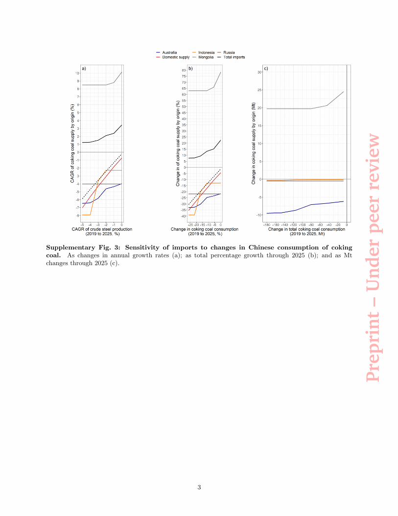
Prep

rin

t–

Un

der

peer

revi

ew

Supplementary Fig. 3: Sensitivity of imports to changes in Chinese consumption of cokingcoal. As changes in annual growth rates (a); as total percentage growth through 2025 (b); and as Mtchanges through 2025 (c).

3

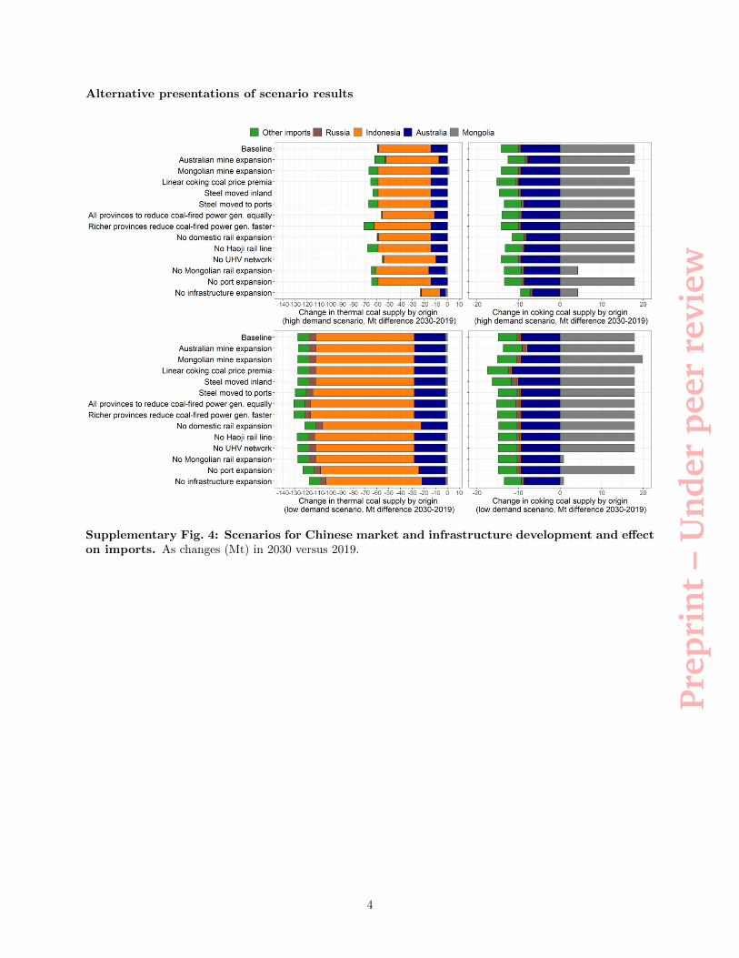
Prep

rin

t–

Un

der

peer

revi

ew

Alternative presentations of scenario results

Supplementary Fig. 4: Scenarios for Chinese market and infrastructure development and effecton imports. As changes (Mt) in 2030 versus 2019.

4

Prep

rin

t–

Un

der

peer

revi

ew

Supplementary Fig. 5: Scenarios for Chinese market and infrastructure development and effecton imports. As total imports (Mt) by 2025.

5

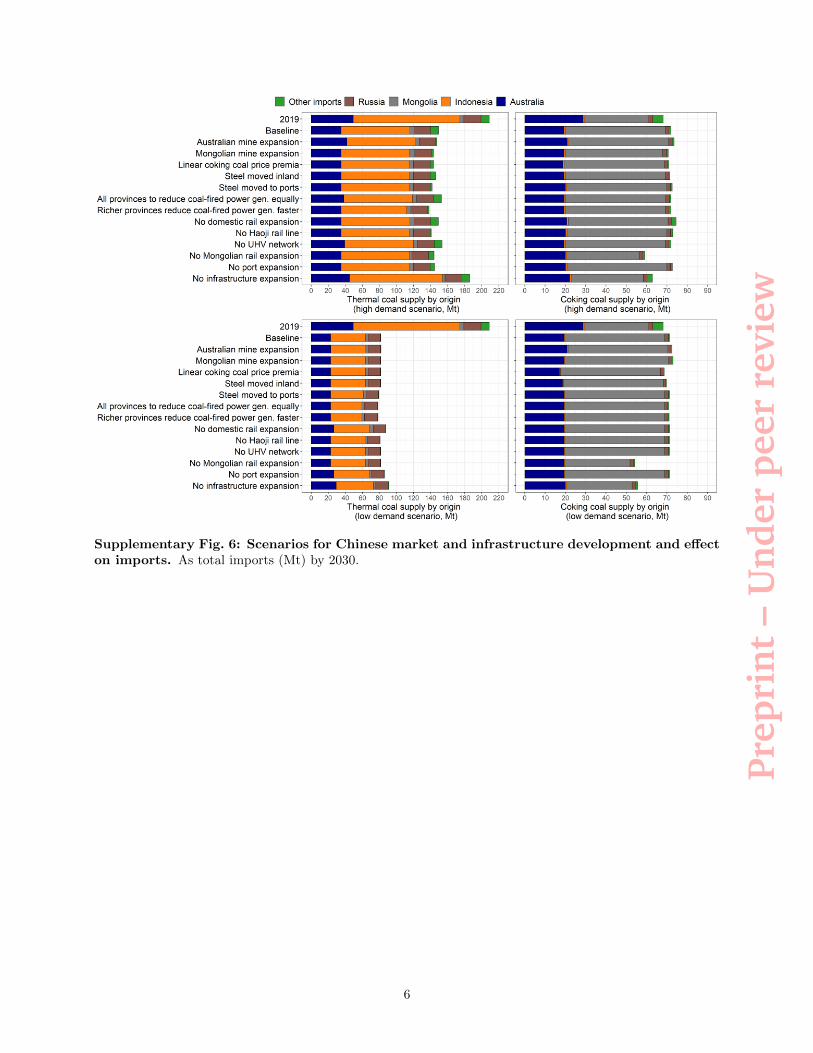
Prep

rin

t–

Un

der

peer

revi

ew

Supplementary Fig. 6: Scenarios for Chinese market and infrastructure development and effecton imports. As total imports (Mt) by 2030.

6

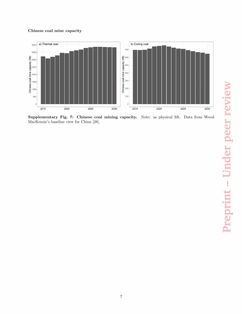
Prep

rin

t–

Un

der

peer

revi

ew

Chinese coal mine capacity

Supplementary Fig. 7: Chinese coal mining capacity. Note: as physical Mt. Data from WoodMacKenzie’s baseline view for China [28].

7

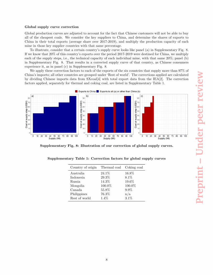
Prep

rin

t–

Un

der

peer

revi

ew

Global supply curve correction

Global production curves are adjusted to account for the fact that Chinese customers will not be able to buyall of the cheapest coals. We consider the key suppliers to China, and determine the shares of exports toChina in their total exports (average share over 2017-2019), and multiply the production capacity of eachmine in those key supplier countries with that same percentage.

To illustrate, consider that a certain country’s supply curve looks like panel (a) in Supplementary Fig. 8.If we know that 20% of this country’s exports over the period 2017-2019 were destined for China, we multiplyeach of the supply steps, i.e., the technical capacity of each individual mine, with that same 20%; panel (b)in Supplementary Fig. 8. That results in a corrected supply curve of that country, as Chinese consumersexperience it, as in panel (c) in Supplementary Fig. 8.

We apply these correction factors to each of the exports of the six countries that supply more than 97% ofChina’s imports; all other countries are grouped under ‘Rest of world’. The corrections applied are calculatedby dividing Chinese imports data from SXcoal[4] with total export data from the IEA[2]. The correctionfactors applied, separately for thermal and coking coal, are listed in Supplementary Table 1.

Supplementary Fig. 8: Illustration of our correction of global supply curves.

Supplementary Table 1: Correction factors for global supply curves

Country of origin Thermal coal Coking coal

Australia 24.1% 16.8%Indonesia 29.3% 8.1%Russia 14.3% 19.6%Mongolia 100.0% 100.0%Canada 55.8% 9.9%Philippines 76.3% n/aRest of world 1.4% 3.1%

8

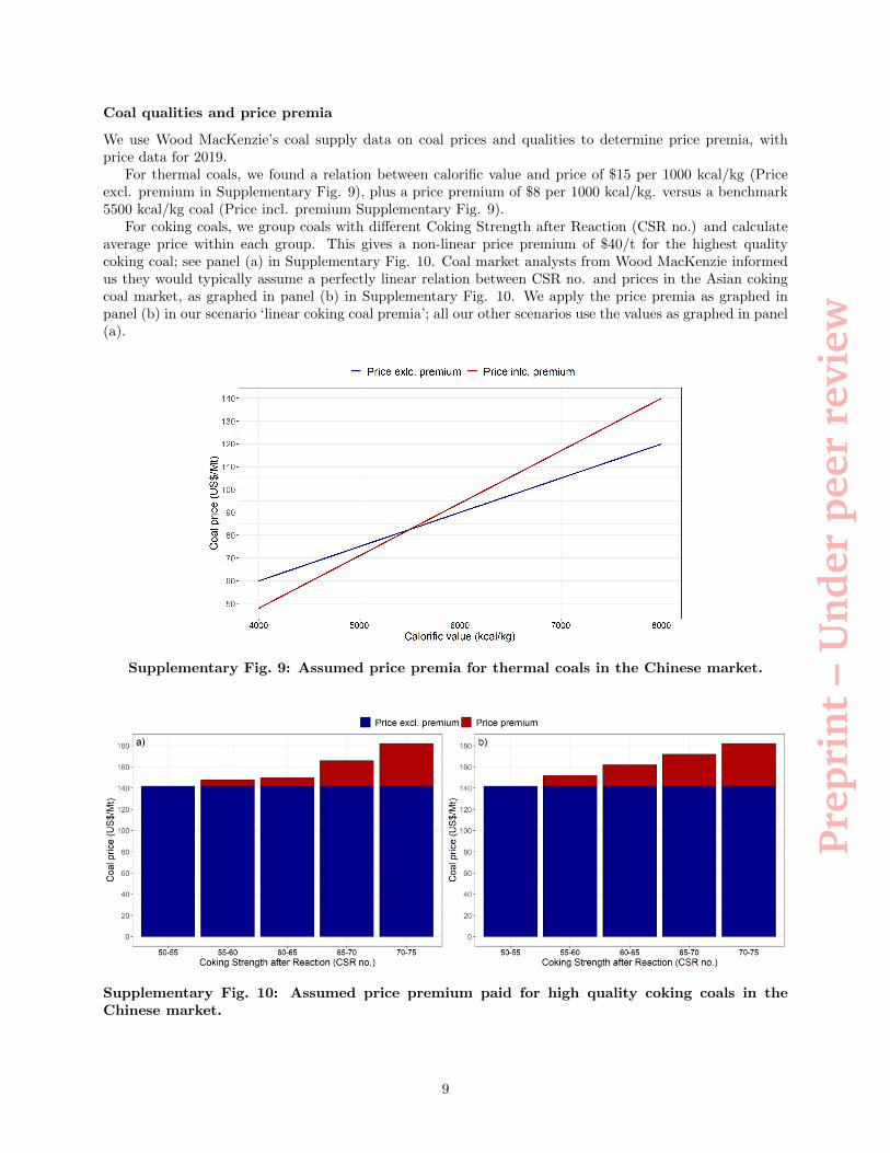
Prep

rin

t–

Un

der

peer

revi

ew

Coal qualities and price premia

We use Wood MacKenzie’s coal supply data on coal prices and qualities to determine price premia, withprice data for 2019.

For thermal coals, we found a relation between calorific value and price of $15 per 1000 kcal/kg (Priceexcl. premium in Supplementary Fig. 9), plus a price premium of $8 per 1000 kcal/kg. versus a benchmark5500 kcal/kg coal (Price incl. premium Supplementary Fig. 9).

For coking coals, we group coals with different Coking Strength after Reaction (CSR no.) and calculateaverage price within each group. This gives a non-linear price premium of $40/t for the highest qualitycoking coal; see panel (a) in Supplementary Fig. 10. Coal market analysts from Wood MacKenzie informedus they would typically assume a perfectly linear relation between CSR no. and prices in the Asian cokingcoal market, as graphed in panel (b) in Supplementary Fig. 10. We apply the price premia as graphed inpanel (b) in our scenario ‘linear coking coal premia’; all our other scenarios use the values as graphed in panel(a).

Supplementary Fig. 9: Assumed price premia for thermal coals in the Chinese market.

Supplementary Fig. 10: Assumed price premium paid for high quality coking coals in theChinese market.

9

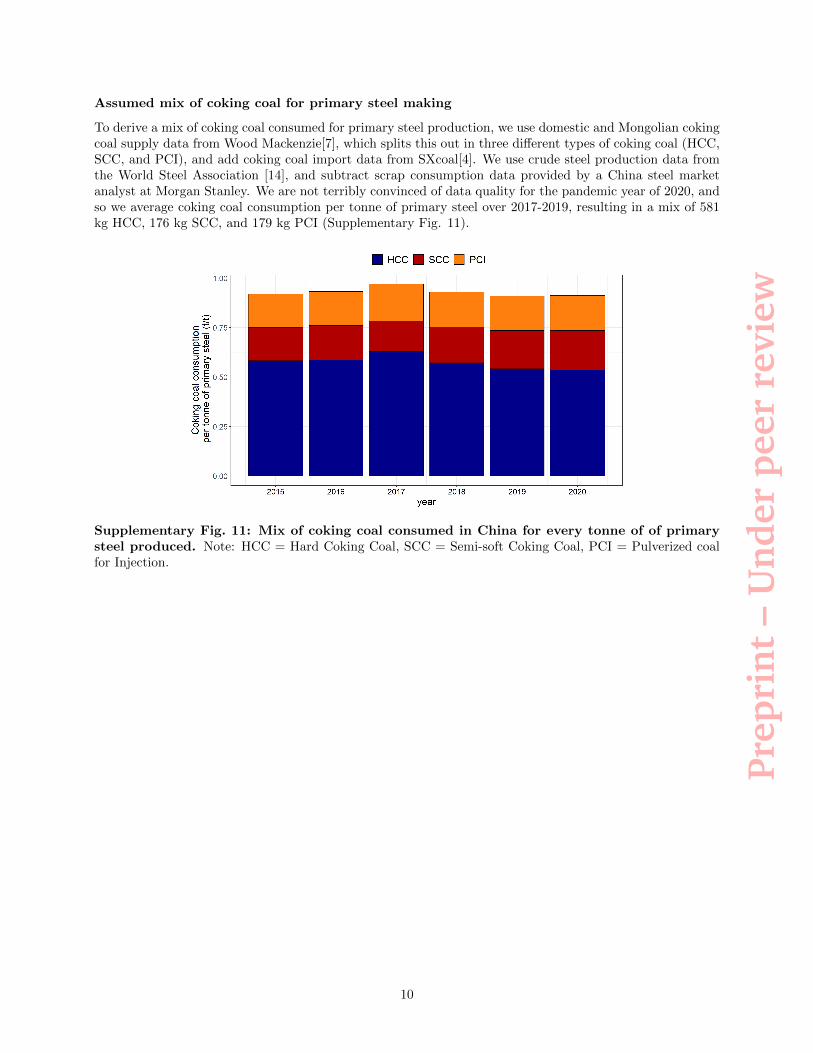
Prep

rin

t–

Un

der

peer

revi

ew

Assumed mix of coking coal for primary steel making

To derive a mix of coking coal consumed for primary steel production, we use domestic and Mongolian cokingcoal supply data from Wood Mackenzie[7], which splits this out in three different types of coking coal (HCC,SCC, and PCI), and add coking coal import data from SXcoal[4]. We use crude steel production data fromthe World Steel Association [14], and subtract scrap consumption data provided by a China steel marketanalyst at Morgan Stanley. We are not terribly convinced of data quality for the pandemic year of 2020, andso we average coking coal consumption per tonne of primary steel over 2017-2019, resulting in a mix of 581kg HCC, 176 kg SCC, and 179 kg PCI (Supplementary Fig. 11).

Supplementary Fig. 11: Mix of coking coal consumed in China for every tonne of of primarysteel produced. Note: HCC = Hard Coking Coal, SCC = Semi-soft Coking Coal, PCI = Pulverized coalfor Injection.

10

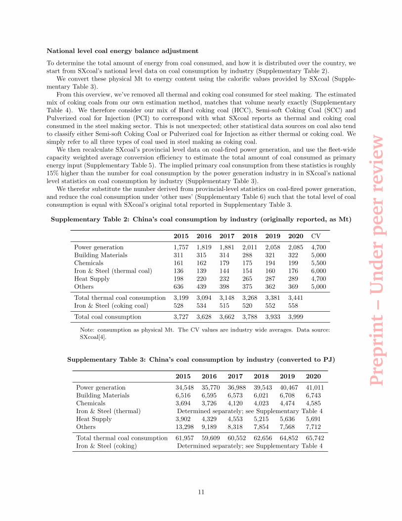
Prep

rin

t–

Un

der

peer

revi

ew

National level coal energy balance adjustment

To determine the total amount of energy from coal consumed, and how it is distributed over the country, westart from SXcoal’s national level data on coal consumption by industry (Supplementary Table 2).

We convert these physical Mt to energy content using the calorific values provided by SXcoal (Supple-mentary Table 3).

From this overview, we’ve removed all thermal and coking coal consumed for steel making. The estimatedmix of coking coals from our own estimation method, matches that volume nearly exactly (SupplementaryTable 4). We therefore consider our mix of Hard coking coal (HCC), Semi-soft Coking Coal (SCC) andPulverized coal for Injection (PCI) to correspond with what SXcoal reports as thermal and coking coalconsumed in the steel making sector. This is not unexpected; other statistical data sources on coal also tendto classify either Semi-soft Coking Coal or Pulverized coal for Injection as either thermal or coking coal. Wesimply refer to all three types of coal used in steel making as coking coal.

We then recalculate SXcoal’s provincial level data on coal-fired power generation, and use the fleet-widecapacity weighted average conversion efficiency to estimate the total amount of coal consumed as primaryenergy input (Supplementary Table 5). The implied primary coal consumption from these statistics is roughly15% higher than the number for coal consumption by the power generation industry in in SXcoal’s nationallevel statistics on coal consumption by industry (Supplementary Table 3).

We therefor substitute the number derived from provincial-level statistics on coal-fired power generation,and reduce the coal consumption under ‘other uses’ (Supplementary Table 6) such that the total level of coalconsumption is equal with SXcoal’s original total reported in Supplementary Table 3.

Supplementary Table 2: China’s coal consumption by industry (originally reported, as Mt)

2015 2016 2017 2018 2019 2020 CV

Power generation 1,757 1,819 1,881 2,011 2,058 2,085 4,700Building Materials 311 315 314 288 321 322 5,000Chemicals 161 162 179 175 194 199 5,500Iron & Steel (thermal coal) 136 139 144 154 160 176 6,000Heat Supply 198 220 232 265 287 289 4,700Others 636 439 398 375 362 369 5,000

Total thermal coal consumption 3,199 3,094 3,148 3,268 3,381 3,441Iron & Steel (coking coal) 528 534 515 520 552 558

Total coal consumption 3,727 3,628 3,662 3,788 3,933 3,999

Note: consumption as physical Mt. The CV values are industry wide averages. Data source:SXcoal[4].

Supplementary Table 3: China’s coal consumption by industry (converted to PJ)

2015 2016 2017 2018 2019 2020

Power generation 34,548 35,770 36,988 39,543 40,467 41,011Building Materials 6,516 6,595 6,573 6,021 6,708 6,743Chemicals 3,694 3,726 4,120 4,023 4,474 4,585Iron & Steel (thermal) Determined separately; see Supplementary Table 4Heat Supply 3,902 4,329 4,553 5,215 5,636 5,691Others 13,298 9,189 8,318 7,854 7,568 7,712

Total thermal coal consumption 61,957 59,609 60,552 62,656 64,852 65,742Iron & Steel (coking) Determined separately; see Supplementary Table 4

11

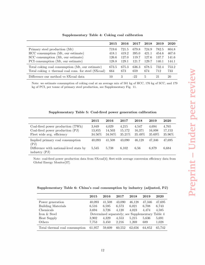
Prep

rin

t–

Un

der

peer

revi

ew

Supplementary Table 4: Coking coal calibration

2015 2016 2017 2018 2019 2020

Primary steel production (Mt) 719.6 721.5 679.8 724.9 782.5 804.8HCC consumption (Mt, our estimate) 418.1 419.2 395.0 421.1 454.6 467.6SCC consumption (Mt, our estimate) 126.6 127.0 119.7 127.6 137.7 141.6PCI consumption (Mt, our estimate) 128.8 129.1 121.7 129.7 140.1 144.1

Total coking coal consumption (Mt, our estimate) 673.5 675.3 636.3 678.5 732.4 753.2Total coking + thermal coal cons. for steel (SXcoal) 664 673 659 674 712 733

Difference our method vs SXcoal data 10 3 -22 5 21 20

Note: we estimate consumption of coking coal at an average mix of 581 kg of HCC, 176 kg of SCC, and 179kg of PCI, per tonne of primary steel production, see Supplementary Fig. 11.

Supplementary Table 5: Coal-fired power generation calibration

2015 2016 2017 2018 2019 2020

Coal-fired power production (TWh) 3,849 4,029 4,215 4,547 4,694 4,765Coal-fired power production (PJ) 13,855 14,503 15,172 16,371 16,898 17,153Fleet wide avg. efficiency 34.56% 34.94% 35.21% 35.49% 35.69% 35.96%

Implied primary coal consumption(PJ)

40,093 41,508 43,090 46,128 47,346 47,695

Difference with national-level stats byindustry (PJ)

5,545 5,738 6,102 6,56 6,879 6,684

Note: coal-fired power production data from SXcoal[4]; fleet-wide average conversion efficiency data fromGlobal Energy Monitor[37].

Supplementary Table 6: China’s coal consumption by industry (adjusted, PJ)

2015 2016 2017 2018 2019 2020

Power generation 40,093 41,508 43,090 46,128 47,346 47,695Building Materials 6,516 6,595 6,573 6,021 6,708 6,743Chemicals 3,694 3,726 4,120 4,023 4,474 4,585Iron & Steel Determined separately; see Supplementary Table 4Heat Supply 3,902 4,329 4,553 5,215 5,636 5,691Others 7,753 3,450 2,216 1,269 689 1,028

Total thermal coal consumption 61,957 59,609 60,552 62,656 64,852 65,742

12

Prep

rin

t–

Un

der

peer

revi

ew

Coal consumption forecasts

For our comparisons in Fig. 6, we use both a low and high demand growth scenario. These are based onthe IEA’s ‘Stated Policies Scenario’ and its ‘Sustainable Development Scenario’. These have previously beenshown to represent the upper and lower range of a suite of demand forecasts from different organizations, ina review by Auger et al[23].

We take the numbers on coal demand from the IEA’s World Energy Outlook 2020[38]. The Annex A tothis report provides forecasts for 2025, and 2030, including separate forecasts for the power generation sector.It does not provide separate forecasts for steel making. For the development of coal consumption in the highdemand scenario, we use a forecast provided to us by a China steel market analyst at Morgan Stanley. Thisforecast presumes a high and extended post-Covid construction stimulus, with total steel demand at 1015Mt in 2025 and 922 Mt in 2030, with a supply of steel from scrap to grow to 290 Mt in 2025, and 322 Mtin 2030, up from 214 Mt in 2019. For the low demand scenario, we use the ‘2 degree compatible’ forecast byWood MacKenzie, which sees total steel demand of 985 Mt in 2025 and 882 Mt in 2030, and use a goal forsteel from scrap of 330 Mt by 2025 and 400 Mt by 2030, taken from a recent policy document by China’sMinistry of Industry and Information Technology[39]. We include these numbers in the IEA’s scenario andthus derive implied growth rates for ‘Other’, which is the growth rates we use for all other industries apartfrom power generation and steel making (Supplementary Tables 7&8).

Supplementary Table 7: Forecasted Chinese coal consumption in the high demand Scenario

CAGR CAGR Total change Total change2019 2025 2030 2019-2025 2019-2030 2019-2025 2019-2030

Power 2,263 2,348 2,324 0.6% 0.2% 3.8% 2.7%Steel 732 679 562 -1.3% -2.4% -7.3% -23.2%Other 837 822 832 -0.3% -0.1% -1.8% -0.6%

Total 3,832 3,849 3,717 0.1% -0.3% 0.4% -3.0%

Note: based on the IEA’s ‘Stated Policies Scenario’ (SPS). For ‘Power’ and ’Other’: thermal coal as Mt ofcoal with an average calorific value of 5,000 kcal/kg coal; for ‘Steel’: as physical Mt of coking coal with a mixas determined in Supplementary Fig. 11.

Supplementary Table 8: Forecasted Chinese coal consumption in the low demand scenario

CAGR CAGR Total change Total change2019 2025 2030 2019-2025 2019-2030 2019-2025 2019-2030

Power 2,263 2,001 1,481 -2.0% -3.8% -11.6% -34.6%Steel 732 612 481 -2.9% -3.8% -16.4% -34.3%Other 837 783 649 -1.1% -2.3% -6.5% -22.4%

Total 3,832 3,396 2,611 -2.0% -3.4% -11.4% -31.9%

Note: based on the IEA’s ‘Sustainable Development Scenario’ (SDS). For ‘Power’ and ‘Other’: thermal coalas Mt of coal with an average calorific value of 5,000 kcal/kg coal; for ‘Steel’: as physical Mt of coking coalwith a mix as determined in Supplementary Fig. 11.

13

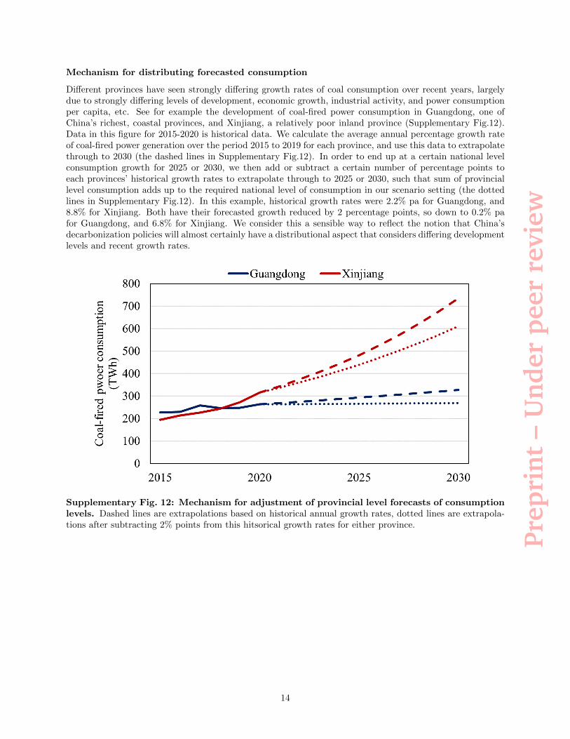
Prep

rin

t–

Un

der

peer

revi

ew

Mechanism for distributing forecasted consumption

Different provinces have seen strongly differing growth rates of coal consumption over recent years, largelydue to strongly differing levels of development, economic growth, industrial activity, and power consumptionper capita, etc. See for example the development of coal-fired power consumption in Guangdong, one ofChina’s richest, coastal provinces, and Xinjiang, a relatively poor inland province (Supplementary Fig.12).Data in this figure for 2015-2020 is historical data. We calculate the average annual percentage growth rateof coal-fired power generation over the period 2015 to 2019 for each province, and use this data to extrapolatethrough to 2030 (the dashed lines in Supplementary Fig.12). In order to end up at a certain national levelconsumption growth for 2025 or 2030, we then add or subtract a certain number of percentage points toeach provinces’ historical growth rates to extrapolate through to 2025 or 2030, such that sum of provinciallevel consumption adds up to the required national level of consumption in our scenario setting (the dottedlines in Supplementary Fig.12). In this example, historical growth rates were 2.2% pa for Guangdong, and8.8% for Xinjiang. Both have their forecasted growth reduced by 2 percentage points, so down to 0.2% pafor Guangdong, and 6.8% for Xinjiang. We consider this a sensible way to reflect the notion that China’sdecarbonization policies will almost certainly have a distributional aspect that considers differing developmentlevels and recent growth rates.

Supplementary Fig. 12: Mechanism for adjustment of provincial level forecasts of consumptionlevels. Dashed lines are extrapolations based on historical annual growth rates, dotted lines are extrapola-tions after subtracting 2% points from this hitsorical growth rates for either province.

14

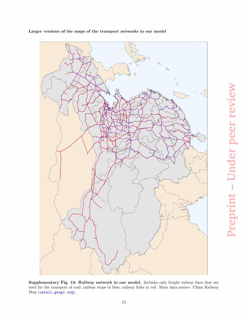
Prep

rin

t–

Un

der

peer

revi

ew

Larger versions of the maps of the transport networks in our model

Supplementary Fig. 13: Railway network in our model. Includes only freight railway lines that areused for the transport of coal; railway stops in blue, railway links in red. Main data source: China RailwayMap (cnrail.geogv.org).

15

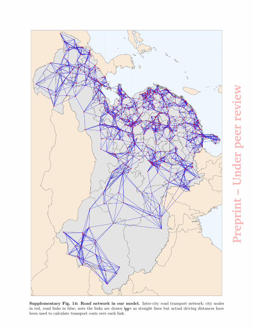
Prep

rin

t–

Un

der

peer

revi

ew

Supplementary Fig. 14: Road network in our model. Inter-city road transport network; city nodesin red, road links in blue; note the links are drawn here as straight lines but actual driving distances havebeen used to calculate transport costs over each link.

16

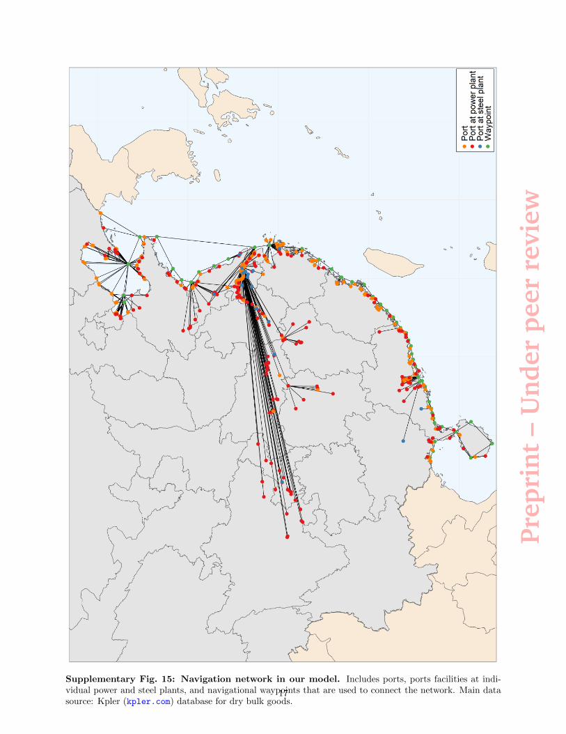
Prep

rin

t–

Un

der

peer

revi

ew

Supplementary Fig. 15: Navigation network in our model. Includes ports, ports facilities at indi-vidual power and steel plants, and navigational waypoints that are used to connect the network. Main datasource: Kpler (kpler.com) database for dry bulk goods.

17

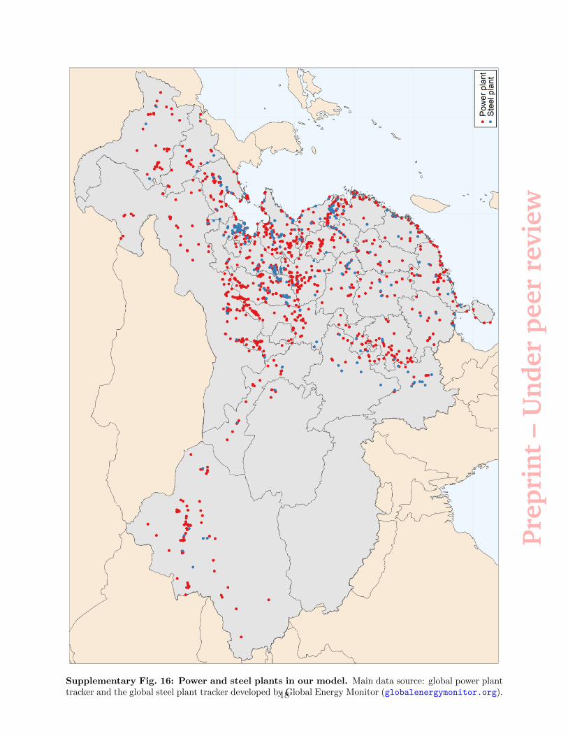
Prep

rin

t–

Un

der

peer

revi

ew

Supplementary Fig. 16: Power and steel plants in our model. Main data source: global power planttracker and the global steel plant tracker developed by Global Energy Monitor (globalenergymonitor.org).18