Preface W - · PDF file18.1 CHAPTER 18 NONRESIDENTIAL COOLING AND HEATING LOAD CALCULATIONS Cooling Load Calculation Principles ..... 18.1

Reprinted and altered with the written permission of ASHRAE and for chapter distribution only.

The publication may not be reproduced without permission from ASHRAE Research Promotion Staff. Patricia Adelmann, Manager – RP 404/636-8400, ext. 1114 or [email protected]

1791 Tullie Circle, Atlanta GA 30329

Preface

What would the world look like without ASHRAE Research? Since its beginnings in 1919,

ASHRAE Research has grown and expanded to address the ever changing questions and topics facing both its members and the HVAC&R Industry and the world as a whole. The ASHRAE Handbook is constantly evolving to address these new challenges, fueled by the knowledge and principals developed through ASHRAE Research. As the focus of the industry has evolved from home refrigeration and food safety to improved indoor air quality to sustainability and energy efficiency, this four-volume series continues to be the cornerstone in every ASHRAE Member’s career.

The power behind ASHRAE Research and the four-volume Handbook comes directly from YOU: your financial support is the driving force behind every research project conducted world wide; your financial investment is an investment in the future of the HVAC&R industry; your donation to ASHRAE Research fills the more than 3,600 Handbook pages.

What would the ASHRAE Handbook look like without your support of ASHRAE Research? Take a look at just one chapter and imagine a world without this guidance from ASHRAE over the last 90 years.

Research Promotion Committee

18.1

CHAPTER 18

NONRESIDENTIAL COOLING AND HEATING LOAD CALCULATIONS

Cooling Load Calculation Principles .. ................................... 18.1Internal Heat Gains .. .............................................................. 18.3Infiltration and Moisture Migration Heat Gains .. ................ 18.11Fenestration Heat Gain ......................................................... 18.14Heat Balance Method . .......................................................... 18.15Radiant Time Series (RTS) Method ....................................... 18.20

Heating Load Calculations . .................................................. 18.28System Heating and Cooling Load Effects ............................ 18.32Example Cooling and Heating Load

Calculations .. .................................................................... 18.36Previous Cooling Load Calculation Methods .. ..................... 18.49Building Example Drawings . ................................................. 18.55

EATING and cooling load calculations are the primary designH basis for most heating and air-conditioning systems and com-ponents. These calculations affect the size of piping, ductwork, dif-fusers, air handlers, boilers, chille rs, coils, compressors, f ans, andevery other component of systems that condition indoor environ-ments. Cooling and heating load calculations can significantly affectfirst cost of building construction, comfort and productivity of occu-pants, and operating cost and energy consumption.

Simply put, heating and cooling loads are the rates of energy in-put (heating) or remo val (cooling) required to maintain an indoorenvironment at a desired temperature and humidity condition. Heat-ing and air conditioning systems are designed, sized, and controlledto accomplish that energy transfer. The amount of heating or coolingrequired at any particular time varies widely, depending on external(e.g., outside temperature) and internal (e.g., number of people oc-cupying a space) factors.

Peak design heating and cooling load calculations, which are thischapter’s focus, seek to determine the maximum rate of heating andcooling energy transfer needed at any point in time. Similar princi-ples, but with different assumptions, data, and application, can beused to estimate b uilding energy con sumption, as described inChapter 19.

This chapter discusses common elements of cooling load calcu-lation (e.g., internal heat gain, ventilation and infiltration, moisturemigration, fenestration heat gain) and two methods of heating andcooling load estimation: heat balance (HB) and radiant time series(RTS).

COOLING LOAD CALCULATION PRINCIPLES

Cooling loads result from many conduction, convection, and radi-ation heat transfer processes through the building envelope and frominternal sources and system components. Buildi ng comp onents orcontents that may affect cooling loads include the following:

• External: Walls, roofs, windo ws, sk ylights, door s, partitio ns,ceilings, and floors

• Internal: Lights, people, appliances, and equipment• Infiltration: Air leakage and moisture migration• System: Outside air, duct leakage and heat gain, reheat, fan and

pump energy, and energy recovery

TERMINOLOGYThe variables affecting cooling load calculations are numerous,

often dif ficult to def ine precisely, and al ways intr icately int erre-lated. Many cooling load components vary widely in magnitude,

and possibly direction, d uring a 24 h period. Because these cyclicchanges in load components often are not in phase with each other,each component must be analyzed to establish the maximum cool-ing load for a building or zone. A zoned system (i.e., one servingseveral independent areas, each w ith its own temperature control)needs to provide no greater total cooling load capacity than the larg-est hourly sum of simultaneous zone loads throughout a design day;however, it must handle the peak c ooling load for each zone at itsindividual peak hour. At some times of day during heating or inter-mediate seasons, some zones ma y requ ire heatin g while othersrequire cooling. The zones’ v entilation, h umidification, or deh u-midification needs must also be considered.

Heat Flow RatesIn air-conditioning design, the following four related heat flow

rates, each of which varies with time, must be differentiated.Space Heat Gain. This instantaneous rate of heat gain is the rate

at which heat enters into and/or is generated within a space. Heatgain is classified by its mode of entry into the space and whether itis sensi ble or la tent. Entry modes include (1) solar radiationthrough transparent surfaces; (2) heat conduction through exteriorwalls and ro ofs; (3) heat conduction through ceilings, floor s, andinterior p artitions; ( 4) heat generated in the spac e by occupants,lights, and appliances; (5) energy transfer through direct-with-spaceventilation and inf iltration of out door air; and (6) miscellaneousheat gains. Sensible heat is added directly to the conditioned spaceby conductio n, con vection, an d/or r adiation. Latent heat ga inoccurs when moisture is added to the space (e.g., from vapor emittedby occupants and equipment). T o maintain a constant hum idityratio, water vapor must condense on the cooling apparatus and beremoved at the same rate it is added to the space. The amount ofenergy required to offset latent heat gain essentially equals the prod-uct of the condensation rate and latent heat of condensation. Inselecting cooling equ ipment, di stinguish between sensible andlatent heat gain: every cooling apparatus has different maximumremoval capacities for sensible versus latent heat for particular oper-ating conditions. In extremely dry climates, humidification may berequired, rather than dehumidification, to maintain thermal comfort.

Radiant Heat Gain. Radiant energy must first be absorbed by sur-faces that enclose the space (walls, floor, and ceiling) and objects inthe space (furniture, etc.). When these surfaces and objects becomewarmer than the surrounding air, some of their heat transfers to theair by convection. The composite heat storage capacity of these sur-faces and objects determines the rate at which their respec tive sur-face temperatures increase for a given radiant input, and thus governsthe relationship between the radiant portion of heat gain and its cor-responding part o f the space cooling load (Figure 1). The therma lstorage effect is critical in differentiating between instantaneous heatgain for a given space and its cooling load at that moment. Predictingthe nature and magnitude of this phenomenon in order to estimate arealistic cooling load for a particular set of circumstances has long

The pr eparation of this chapter is a ssigned to T C 4.1, Load C alculationData and Procedures.

18.2 2009 ASHRAE Handbook—Fundamentals

been of inter est to design engineers; the Bibliogr aphy lists someearly work on the subject.

Space Cooling Load. This is the rate at which sensible and latentheat must be removed from the space to maintain a constant spaceair temperature and humidity. The sum of all space instantaneousheat gains at an y gi ven time doe s not necessarily (or e ven fre-quently) equal the cooling load for the space at that same time.

Space Heat E xtraction Rate. The rates at which sensible andlatent heat are removed from the conditioned space equal the spacecooling load only if the room air temperature and humidity are con-stant. Along with the intermittent operation of cooling equipment,control systems usually allow a minor cyclic variation or swing inroom temperature; humidity is often allowed to float, but it can becontrolled. Therefore, proper simulation of the control system givesa more realistic value of energy removal over a f ixed period thanusing values of the space cooling load. However, this is primarilyimportant for esti mating energy use over time; it is not needed tocalculate design peak cooling load for equipment selection.

Cooling Coil Load. The rate at which energy is re moved at acooling coil serving one or more conditioned spaces equals the sumof instantaneous space cooling loads (or space heat extraction rate,if it is assumed that space temperature and humidity vary) for allspaces se rved by the c oil, plus any s ystem l oads. Sys tem loadsinclude fan heat gain, duct heat gain, and outdoor air heat and mois-ture brought into the cooling equipment to satisfy the ventilation airrequirement.

Time Delay EffectEnergy absorbed by w alls, floor, furniture, etc., contributes to

space cooling load only after a time lag. Some of this energy is stillpresent and rer adiating e ven after the heat sources ha ve beenswitched off or removed, as shown in Figure 2.

There is always significant delay between the time a heat sourceis activated, and the point when reradiated energy equals that beinginstantaneously stored. This time lag must be considered when cal-culating cooling load, because the load required for the space can bemuch lower than the instantaneous heat gain being generated, andthe space’s peak load may be significantly affected.

Accounting for th e time delay ef fect is the major challenge incooling load calculations. Several methods, including the two pre-sented in this chapter, have been developed to take the time delayeffect into consideration.

COOLING LOAD CALCULATION METHODSThis chapter presents two load calculation methods that vary sig-

nificantly from previous methods. The technology involved, how-ever (the principle of calculating a heat balance for a given space) isnot new. The f irst of the tw o methods is th e heat balance (HB)method; the second is radiant time series (RTS), which is a sim-plification of the HB procedure. Both methods are explained in theirrespective sections.

Cooling load calculation of an ac tual, mul tiple-room buildingrequires a complex computer program implementing the principlesof either method.

Cooling Load Calculations in PracticeLoad calculations sh ould accurately descri be the building. All

load calculation inputs should be as accurate as reasonable, withoutusing safety f actors. Introd ucing compounding safety f actors atmultiple levels in the load calculation results in an unrealistic andoversized load.

Variation in h eat tra nsmission coe fficients of typ ical b uildingmaterials and com posite a ssemblies, dif fering moti vations andskills of those who construct the building, unknown filtration rates,and the manner in which the building is actually operated are someof the variables that make precise calculation impossible. Ev en ifthe designer uses reasonable procedures to account for these factors,the calculation can never be more than a good estimate of the actualload. Frequently, a c ooling load must be ca lculated be fore everyparameter in the conditioned space can be properly o r completelydefined. An example is a cooling load estimate for a new buildingwith many floors of unleased sp aces for which de tailed partitionrequirements, furnis hings, ligh ting, and layout cannot be pre-defined. Potential tenant mod ifications once the building is occu-pied a lso must be con sidered. Load estimating r equires properengineering judgment that in cludes a tho rough understanding ofheat balance fundamentals.

Perimeter spaces exposed to high solar heat gain often need cool-ing during sunlit portions of traditional heating months, as do com-pletely inter ior spaces with significant internal heat gain. Thesespaces can also ha ve signif icant heating loads during nonsunlithours or after periods of nonoccupancy, when adjacent spaces havecooled belo w interior design te mperatures. The hea ting loadsinvolved can be estimated conventionally to offset or to compensatefor them and prevent overheating, but they have no direct relation-ship to the spaces’ design heating loads.

Correct design and sizing of ai r-conditioning systems requiremore than calculation of the coolin g load in the space to be condi-tioned. The type of ai r-conditioning system, ventilation rate, reheat,fan energy, fan location, duct heat loss and gain, duct leakage, heatextraction lighting systems, type of return air system, and any sensibleor latent heat recovery all affect system load and component sizing.Adequate system design and component sizing require that systemperformance be analyzed as a series of psychrometric processes.

System design could be driven by either sensible or latent load, andboth need to be checked. When a space is sensible-load-driven, whichis generally the case, the cooling supply air will have surplus capacityto dehumidify, but this is commonly permissible. For a space drivenby latent load, (e.g., an auditorium), supply airflow based on sensibleload is likely not have enough dehumidifying capability, so subcool-ing and reheating or some other dehumidification process is needed.

This chapter is primarily concerned with a given space or zone ina building. When estimating loads for a group of spaces (e.g., for an

Fig. 1 Origin of Difference Between Magnitude of Instanta-neous Heat Gain and Instantaneous Cooling Load

Fig. 1 Origin of Difference Between Magnitude of Instantaneous Heat Gain and Instantaneous Cooling Load

Fig. 2 Thermal Storage Effect in Cooling Load from Lights

Fig. 2 Thermal Storage Effect in Cooling Load from Lights

Nonresidential Cooling and Heating Load Calculations 18.3

air-handling system that serv es m ultiple z ones), the a ssembledzones must be analyzed to consider (1) the simultaneous effects tak-ing place; (2) any diversification of heat gains for occupants, light-ing, or other internal load sources; (3) ventilation; and/or (4) anyother unique circumstances. With large buildings that involve morethan a single HVAC system, simultaneous loads and any additionaldiversity also must be considered when designing the central equip-ment that serves the systems. Methods presented in this chapter areexpressed as hourly load summaries, reflecting 24 h input schedulesand profiles of the indi vidual load variables. Specific systems andapplications may require different profiles.

DATA ASSEMBLYCalculating space cooling loads requires detailed building design

information and weather data at design conditions. Generally, thefollowing information should be compiled.

Building Characteristics. Building materials, component size,external sur face colors, and shape are usually determined frombuilding plans and specifications.

Configuration. Determine building location, ori entation, andexternal shading from building plans and specifications. Shadingfrom adjacent buildings can be determined from a site plan or byvisiting the proposed site, but its probable permanence should becarefully evaluated before it is included in the calculation. Thepossibility of abnormally high ground-reflected solar radiation(e.g., from adjacent water, sand, or parking lots) or solar load fromadjacent reflective buildings should not be overlooked.

Outdoor Design Conditions. Obtain appropriate weather data,and select outdoor design conditions. Chapter 14 provides infor-mation for many weather stations; note, however, that these designdry-bulb and mean coincident wet-bulb temperatures may varyconsiderably from data traditi onally used in v arious areas. Usejudgment to ensure that results are consistent with e xpectations.Also, consider prevailing wind velocity and the re lationship of aproject site to the selected weather station.

Recent research projects have greatly expanded the amount ofavailable weather data (e.g., AS HRAE 2004). In addition to theconventional dry-b ulb with mean coincident wet -bulb, dat a arenow available for wet-bulb and dew point with mean coincidentdry-bulb. Peak space load generally coincides with peak solar orpeak dry-bulb, but peak system load often occurs at peak wet-bulbtemperature. The relationship between space and system loads isdiscussed further in following sections of the chapter.

To estimate conductive heat gain through exterior surfaces andinfiltration and outdoor air load s at an y time, applicable outdoordry- and wet-b ulb te mperatures must be used. Chapter 1 4 gi vesmonthly cooling load design values of outdoor conditions for manylocations. These are generally midafternoon conditions; for othertimes of day, the daily range profile method described in Chapter 14can be used to estimate dry- and wet-bulb temperatures. Peak cool-ing load is often determined by solar heat gain through fenestration;this peak may occur in winter months and/or at a time of day whenoutside air temperature is not at its maximum.

Indoor Design Conditions. Select indoor dry-bulb temperature,indoor relative humidity, and v entilation rate. Include permissiblevariations and control limits. Consult ASHRAE Standard 90.1 forenergy-savings conditions, and Standard 55 for r anges of indoorconditions needed for thermal comfort.

Internal Heat Gains a nd Op erating Sch edules. Obta inplanned density and a proposed schedule of lighting, occupancy,internal equipment, appliances, and processes that contribute to theinternal thermal load.

Areas. Use consistent methods for calculation of building areas.For fenestration, the definition of a component’s area must be con-sistent with associated ratings.

Gross surface area. It is efficient and conservative to derive grosssurface areas from outside building dimensions, ignoring wall andfloor thicknesses and avoiding separate accounting of floor edge andwall corner conditions. Measure floor areas to the outside of adjacentexterior w alls or to the center line of adjacent partitions. Whenapportioning to ro oms, f açade area sh ould be divided at partitioncenter lines. Wall height should be taken as floor-to-floor height.

The outside-dimension procedure is expedient for load calcula-tions, but it is not consistent with rigorous definitions used in build-ing-related standards. The resulting d ifferences d o no t introducesignificant errors in this chapter’s procedures.

Fenestration area. As d iscussed in Chapter 15, fenestration rat-ings [U-factor and solar heat gain coefficient (SHGC)] are based onthe entire product area, including frames. Thus, for load calculations,fenestration area is the area of the rough opening in the wall or roof.

Net surface area. Net surface area is the gross surface area lessany enclosed fenestration area.

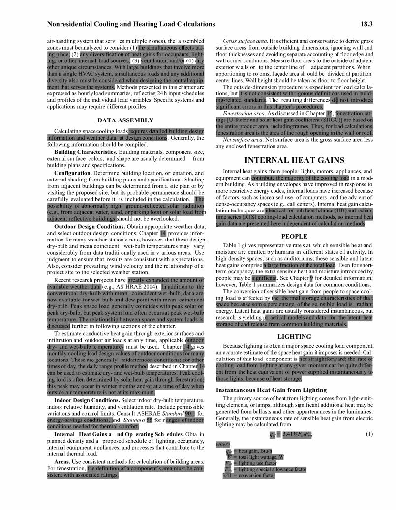
INTERNAL HEAT GAINSInternal heat g ains from people, lights, motors, appliances, and

equipment can contribute the majority of the cooling load in a mod-ern building. As b uilding envelopes have improved in resp onse tomore restrictive energy codes, internal loads have increased becauseof f actors such as increa sed use of computers and the adv ent ofdense-occupancy spaces (e.g., call centers). Internal heat gain calcu-lation techniques are identical for both heat balance (HB) and radianttime series (RTS) cooling-load calculation methods, so internal heatgain data are presented here independent of calculation methods.

PEOPLETable 1 gi ves representati ve rate s at whi ch se nsible he at and

moisture a re emitted by humans in different states of activity. Inhigh-density spaces, such as auditoriums, these sensible and latentheat gains comprise a large fraction of the total load. Even for short-term occupancy, the extra sensible heat and moisture introduced bypeople may be significant. See Chapter 9 for detailed information;however, Table 1 summarizes design data for common conditions.

The conversion of sensible heat gain from people to space cool-ing load is af fected by the thermal storage characteristics of tha tspace bec ause som e perc entage of the se nsible load is radiantenergy. Latent heat gains are usually considered instantaneous, butresearch is yielding pr actical models and data for the latent heatstorage of and release from common building materials.

LIGHTINGBecause lighting is often a major space cooling load component,

an accurate estimate of the space heat gain it imposes is needed. Cal-culation of this load component is not straightforward; the rate ofcooling load from lighting at any given moment can be quite differ-ent from the heat equivalent of power supplied instantaneously tothose lights, because of heat storage.

Instantaneous Heat Gain from LightingThe primary source of heat from lighting comes from light-emit-

ting elements, or lamps, although significant additional heat may begenerated from ballasts and other appurtenances in the luminaires.Generally, the instantaneous rate of sensible heat gain from electriclighting may be calculated from

qel = 3.41WFulFsa (1)

whereqel = heat gain, Btu/hW = total light wattage, W

Ful = lighting use factorFsa = lighting special allowance factor

3.41 = conversion factor

18.4 2009 ASHRAE Handbook—Fundamentals

The total light wattage is obtained from the ratings of all lampsinstalled, both for general illumination and for display use. Ballastsare not included, but are addressed by a separate factor. Wattages ofmagnetic ballasts are significant; the energy consumption of high-efficiency el ectronic bal lasts m ight be insignif icant compared tothat of the lamps.

The lighting use factor is the ratio of wattage in use, for the con-ditions under which the load estimate is being made, to totalinstalled wattage. For commercial applications such as store s, theuse factor is generally 1.0.

The special allowance factor is the ratio of the lighting fixtures’power consumption, including la mps and ballast, to the nom inalpower consumption of the lamps. For incandescent lights, this factoris 1. For fluorescent lights, it accounts for power consumed by theballast as well as the ballast’s effect on lamp po wer consumption.The special allowance factor can be less than 1 for electronic bal-lasts tha t lo wer el ectricity consum ption below the lamp’s rate dpower consumption. Use manufacturers’ values for system (lamps +ballast) power, when available.

For high-intensity-discharge lamps (e.g. metal halide, mercuryvapor, high- and low-pressure sodium vapor lamps), the actual light-ing system power consumption should be available from the manu-facturer of the fixture or ballast. Ballasts available for metal halideand high pressure sodium vapor lamps may have special allowancefactors from about 1.3 (for low-wattage lamps) do wn to 1.1 (forhigh-wattage lamps).

An alternative procedure is to estimate the lighting heat gain on aper square foot basis. Such an approach may be required when finallighting plans are not available. Table 2 shows the maximum lightingpower density (LPD) (lighting heat gain per square foot) allowed byASHRAE Standard 90.1-2007 for a range of space types.

In addition to determining the lighting heat gain, the fraction oflighting heat gain that enters the conditioned space may need to bedistinguished from the fraction that enters an unconditioned space;of the former category, the distribution between radiative and con-vective heat gain must be established.

Fisher and Chantrasrisalai (2006) experimentally studied 12 lumi-naire types and recommended five different categories of luminaires,

as shown in Table 3. The table provides a range of design data for theconditioned space fraction, short-wave radiative fraction, and long -wave radiative fraction under typical operating conditions: airflowrate of 1 cfm/ft², supply air temperature between 59 and 62°F, an droom air temperature between 72 and 75°F. The recommended frac-tions in Table 3 are based on lighting heat input rates range of 0.9 to2.6 W/ft2. For higher design power input, the lower bounds of thespace and short -wave fractions should be used; for design po werinput below this range, the upper bounds of the space and short-wavefractions should be used. The space fraction in the table is the frac-tion of lighting heat gain that goes to the room; the fraction going tothe plenum can be computed as 1 – the space fraction. The radiativefraction is the radiative part of the lighting heat gain that goes to theroom. The convective fraction of the lighting heat gain that goes tothe room is 1 – the radiative fraction. Using values in the middle ofthe range yields sufficiently accurate results. However, values thatbetter suit a specific situation may be determined according to thenotes for Table 3.

Table 3’ s data are applicab le for both ducted and nonductedreturns. However, application of the data, particularly the ceilingplenum fraction, may vary for different return configurations. Forinstance, for a room with a ducted return, although a portion of thelighting energy initially dissipated to the ceiling plenum is quanti-tatively equal to the plenum fraction, a large portion of this energywould likely end up as the condi tioned space cooling load and asmall portion would end up as the cooling load to the return air.

If the space airflow rate is different from the typical condition(i.e., about 1 cfm/ft²), Figure 3 can be used to estimate the lightingheat gain parameters. Design data shown in Figure 3 are only appli-cable for the recessed fluorescent luminaire without lens.

Although design data presented in Table 3 and Figure 3 can beused for a vented luminaire with side-slot returns, they are likely notapplicable for a vented luminaire with la mp compartment returns,because in the latter case, all heat convected in the vented luminaireis likely to go directly to the ceiling plenum, resulting in zero con-vective fra ction and a much lo wer space fract ion. Therefore, thedesign data sh ould only be u sed for a con figuration where condi-tioned air is returned through the ceiling grille or luminaire side slots.

Table 1 Representative Rates at Which Heat and Moisture Are Given Off by Human Beings in Different States of Activity

Degree of Activity Location

Total Heat, Btu/h Sensible Heat,Btu/h

Latent Heat,Btu/h

% Sensible Heat that is Radiantb

AdultMale

Adjusted, M/Fa Low V High V

Seated at theater Theater, matinee 390 330 225 105Seated at theater, night Theater, night 390 350 245 105 60 27Seated, very light work Offices, hotels, apartments 450 400 245 155

Moderately active office work Offices, hotels, apartments 475 450 250 200Standing, light work; walking Department store; retail store 550 450 250 200 58 38Walking, standing Drug store, bank 550 500 250 250Sedentary work Restaurantc 490 550 275 275

Light bench work Factory 800 750 275 475Moderate dancing Dance hall 900 850 305 545 49 35Walking 3 mph; light machine work Factory 1000 1000 375 625

Bowlingd Bowling alley 1500 1450 580 870Heavy work Factory 1500 1450 580 870 54 19Heavy machine work; lifting Factory 1600 1600 635 965Athletics Gymnasium 2000 1800 710 1090Notes:1. Tabulated values are based on 75°F room dry-bulb temperature. For 80°F room dry

bulb, total heat remains the same, but sensible heat values should be decreased byapproximately 20%, and latent heat values increased accordingly.

2. Also see Table 4, Chapter 9, for additional rates of metabolic heat generation.3. All values are rounded to nearest 5 Btu/h.aAdjusted heat gain is based on normal percentage of men, women, and childrenfor the application listed, and assumes that gain from an adult female is

85% of that for an adult male, and gain from a child is 75% of that for an adult male.b Values approximated from data in Table 6, Chapter 9, where V is air velocity with limitsshown in that table.

cAdjusted heat gain includes 60 Btu/h for f ood per individual (30 Btu/h sensible and 3 0Btu/h latent).

d Figure one person per alley actually bowling, and all others as sitting (400 Btu/h) or stand-ing or walking slowly (550 Btu/h).

Nonresidential Cooling and Heating Load Calculations 18.5

Table 2 Lighting Power Densities Using Space-by-Space Method

Common Space Types* LPD, W/ft2 Building-Specific Space Types LPD, W/ft2

Office—enclosed 1.1 Gymnasium/exercise centerOffice—open plan 1.1 Playing Area 1.4Conference/meeting/multipurpose 1.3 Exercise Area 0.9Classroom/lecture/training 1.4 Courthouse/police station/penitentiary

For penitentiary 1.3 Courtroom 1.9Lobby 1.3 Confinement cells 0.9

For hotel 1.1 Judges’ chambers 1.3For performing arts theater 3.3 Fire StationsFor motion picture theater 1.1 Engine room 0.8

Audience/seating Area 0.9 Sleeping quarters 0.3For gymnasium 0.4 Post office—sorting area 1.2For exercise center 0.3 Convention center—exhibit space 1.3For convention center 0.7 LibraryFor penitentiary 0.7 Card file and cataloging 1.1For religious buildings 1.7 Stacks 1.7For sports arena 0.4 Reading area 1.2For performing arts theater 2.6 HospitalFor motion picture theater 1.2 Emergency 2.7For transportation 0.5 Recovery 0.8

Atrium—first three floors 0.6 Nurses’ station 1.0Atrium—each additional floor 0.2 Exam/treatment 1.5Lounge/recreation 1.2 Pharmacy 1.2

For hospital 0.8 Patient room 0.7Dining Area 0.9 Operating room 2.2

For penitentiary 1.3 Nursery 0.6For hotel 1.3 Medical supply 1.4For motel 1.2 Physical therapy 0.9For bar lounge/leisure dining 1.4 Radiology 0.4For family dining 2.1 Laundry—washing 0.6

Food preparation 1.2 Automotive—service/repair 0.7Laboratory 1.4 ManufacturingRestrooms 0.9 Low bay (<25 ft floor to ceiling height) 1.2Dressing/locker/fitting room 0.6 High bay (≥25 ft7.6 m floor to ceiling height) 1.7Corridor/transition 0.5 Detailed manufacturing 2.1

For hospital 1.0 Equipment room 1.2For manufacturing facility 0.5 Control room 0.5

Stairs—active 0.6 Hotel/motel guest rooms 1.1Active storage 0.8 Dormitory—living quarters 1.1

For hospital 0.9 MuseumInactive storage 0.3 General exhibition 1.0

For museum 0.8 Restoration 1.7Electrical/mechanical 1.5 Bank/office—banking activity area 1.5Workshop 1.9 Religious buildingsSales area [for accent lighting, see Section 9.6.2(B) of

ASHRAE Standard 90.1]1.7 Worship pulpit, choir 2.4

Fellowship hall 0.9Retail

Sales area for accent lighting, see Section 9.6.3(C) of ASHRAE Standard 90.1]

1.7

Mall concourse 1.7Sports arena

Ring sports area 2.7Court sports area 2.3Indoor playing field area 1.4

WarehouseFine material storage 1.4Medium/bulky material storage 0.9

Parking garage—garage area 0.2Transportation

Airport—concourse 0.6Air/train/bus—baggage area 1.0Terminal—ticket counter 1.5

Source: ASHRAE Standard 90.1-2007.*In cases where both a common space type and a building-specific type are listed, the building-specific space type applies.

18.6 2009 ASHRAE Handbook—Fundamentals

For other luminaire types, it ma y be nec essary to esti mate theheat gain for each component as a fraction of the total lighting heatgain by using judgment to estimate heat-to-space and heat-to-returnpercentages.

Because of the directional na ture of downlight l uminaires, alarge portion of the short-wave radiation typically falls on the floor.When converting heat gains to cooling loads in the RTS method, thesolar radiant time factors (RTF) may be more appropriate than non-solar RTF. (Solar RTF are calculated assuming most solar radiationis intercepted by the floor; nonsolar RTF assume uniform distribu-tion by area over all interior surfaces.) This effect may be significantfor rooms where lighting heat gain is high and for which solar RTFare significantly different from nonsolar RTF.

ELECTRIC MOTORSInstantaneous sensible h eat g ain fr om equip ment op erated by

electric motors in a conditioned space is calculated asqem = 2545(P/EM)FUM FLM (2)

whereqem = heat equivalent of equipment operation, Btu/h

P = motor power rating, hpEM = motor efficiency, decimal fraction <1.0

FUM = motor use factor, 1.0 or decimal fraction <1.0FLM = motor load factor, 1.0 or decimal fraction <1.0

2545 = conversion factor, Btu/h·hp

The motor use factor may be applied when motor use is known tobe intermittent, with significant nonuse during all hours of operation(e.g., o verhead door oper ator). F or conventional applicatio ns, itsvalue is 1.0.

The motor load factor is the fraction of the rated load deliveredunder the conditions of the cooling load estimate. In Equation (2), itis assumed that both the motor and driven equipment are in the con-ditioned space. If the motor is outside the space or airstream,

qem = 2545PFUM FLM (3)

When the motor is inside the conditioned space or airstream butthe driven machine is outside,

(4)

Equation (4) also applies to a f an or pump in the conditionedspace that exhausts air or pumps fluid outside that space.

Table 4 gives minimum efficiencies and related data representa-tive of typical electric motors from ASHRAE Standard 90.1-2007.If electric motor load is an appreciable portion of cooling load, themotor efficiency should be obtained from the manufacturer. Also,depending on design , maximum ef ficiency might occur an ywherebetween 75 to 110% of full load; if under- or o verloaded, effi-ciency could vary from the manufacturer’s listing.

Overloading or UnderloadingHeat output of a motor is generally proportional to motor load,

within rated o verload limits. Because of typically high no-loadmotor cur rent, f ixed losses, and other reasons, FLM is general lyassumed to be unity, and no adjustment should be made for under-loading or o verloading unless th e situation is f ixed and can beaccurately establ ished, and reduced-load ef ficiency data can beobtained from the motor manufacturer.

Radiation and ConvectionUnless the m anufacturer’s t echnical li terature indicates other-

wise, motor heat gain normally should be equally divided betweenradiant and convective components for the subsequent cooling loadcalculations.

APPLIANCESA cooling load estimate should take into account heat gain from

all appliances (electrical, gas, or steam). Because of the variety ofappliances, applications, schedules, use, and installations, estimatescan be very subjective. Often, the only information available about

Fig. 3 Lighting Heat Gain Parameters for Recessed Fluores-cent Luminaire Without Lens

Fig. 3 Lighting Heat Gain Parameters for Recessed Fluorescent Luminaire Without Lens

(Fisher and Chantrasrisalai 2006)

qem 2545P1.0 EM–

EM---------------------

⎝ ⎠⎜ ⎟⎛ ⎞

FUM FLM=

Table 3 Lighting Heat Gain Parameters for Typical Operating ConditionsLuminaire Category Space Fraction Radiative Fraction Notes

Recessed fluorescent luminaire without lens

0.64 to 0.74 0.48 to 0.68 • Use middle values in most situations• May use higher space fraction, and lower radiative fraction for luminaire

with side-slot returns• May use lower values of both fractions for direct/indirect luminaire• May use higher values of both fractions for ducted returns

Recessed fluorescent luminaire with lens

0.40 to 0.50 0.61 to 0.73 • May adjust values in the same way as for recessed fluorescent luminairewithout lens

Downlight compact fluorescent luminaire

0.12 to 0.24 0.95 to 1.0 • Use middle or high values if detailed features are unknown• Use low value for space fraction and high value for radiative fraction if

there are large holes in luminaire’s reflectorDownlight incandescent

luminaire0.70 to 0.80 0.95 to 1.0 • Use middle values if lamp type is unknown

• Use low value for space fraction if standard lamp (i.e. A-lamp) is used• Use high value for space fraction if reflector lamp (i.e. BR-lamp) is used

Non-in-ceiling fluorescent luminaire

1.0 0.5 to 0.57 • Use lower value for radiative fraction for surface-mounted luminaire• Use higher value for radiative fraction for pendant luminaire

Source: Fisher and Chantrasrisalai (2006).

Nonresidential Cooling and Heating Load Calculations 18.7

heat gain from equipment is that on its nameplate, which can over-estimate actual heat gain for many types of appliances, as discussedin the section on Office Equipment.

Cooking AppliancesThese appliances include common heat-p roducing coo king

equipment found in conditioned commercial kitchens. Marn (1962)concluded that appliance surf aces contributed most of the heat tocommercial kitchens and that when appliances were installed underan effective hood, the co oling load w as independent o f the fuel orenergy used for similar equipment performing the same operations.

Gordon et al. (1994) and Smith et al. (1995) found that gas appli-ances may exhibit slightly higher heat gains than their electric coun-terparts under w all-canopy hoods operated at t ypical v entilationrates. Th is is b ecause heat c ontained in co mbustion pr oducts e x-hausted from a gas appliance may increase the temperatures of theappliance and surrounding surfaces, as well as the ho od above theappliance, more so than the heat produced by its electric counterpart.These higher-temperature surfaces radiate heat to the kitchen, addingmoderately to the radiant gain directly associated with the appliancecooking surface.

Marn (1962) conf irmed that, wh ere appliances are installedunder an effective hood, only radiant gain adds to the cooling load;convective and latent heat from cooking and combustion productsare exhausted and do not enter the kitchen. Gordon et al. (1994) andSmith et al. (1995) substantiated these findings. Chapter 31 of the2007 ASHRAE Handbook—HVAC Applications has more informa-tion on kitchen ventilation.

Sensible Heat G ain f or H ooded Cooking A ppliances. Toestablish a heat gain value, nameplate energy input ratings may beused with appropriate usage and radiation factors. Where specificrating data are not available (nameplate missing, equipment not yetpurchased, etc.), representative heat gains listed in Tables 5A to E(Swierczyna et al. 200 8, 2009 ) fo r a wid e variety of commonlyencountered equipment items. In estimating appliance load, proba-bilities of simultaneous use an d operation for dif ferent applianceslocated in the same space must be considered.

Radiant heat gain from hooded cooking equipment can rangefrom 15 to 45% of the actual appliance energy consumption (Gor-don et al. 1994; Smith et al. 1995; Swierczyna et al. 2008; Talbert etal. 1973). This ratio of heat gain to appliance energy consumptionmay be expressed as a radiation factor, and it is a function of bothappliance type and fuel source. The radiation factor FR is applied tothe average rate of a ppliance energy consumption, determined byapplying usage factor FU to the nameplate or rated ener gy input.Marn (1962) found that radiant heat temperature rise can be sub-stantially reduced by shielding the fronts of cook ing appliances.Although this approach may not always be practical in a commer-cial kitchen, radiant gains can also be reduced by adding side panelsor partial enclosures that are integrated with the exhaust hood.

Heat Gain fr om Meals. For each meal serv ed, approximately50 Btu/h of heat, of which 75% is sensible and 25 % is la tent, istransferred to the dining space.

Heat Gain for Generic Appliances. The average rate of appli-ance energy consumption can be estimated from the nameplate orrated energy input qinput by applying a duty cycle or usage factor FU.Thus, sensible heat gain qs for generic electric, steam, and gas appli-ances installed under a hood can be estimated using one of the fol-lowing equations:

qs = qinput FU FR (5)

or

qs = qinput FL (6)

where FL is the rat io of sensible hea t ga in to the ma nufacturer’srated energy input. However, recent ASHRAE research (Swierc-zyna et al. 2008, 2009) showed the design value for heat gain froma hooded appliance at idle (ready-to-cook) conditions based on itsenergy consumption rate is, at best, a rough estimate. When appli-ance heat gain measurements during idle conditions were regressedagainst energy consumption rates for gas and electr ic appliances,the a ppliances’ emissivity, insul ation, and surf ace cooling (e.g.,through v entilation rate s) scattered the data points widely , withlarge deviations from the average values. Because large errors couldoccur in the heat load ca lculation for spec ific appliance lines byusing a general radiation factor, heat gain values in Table 5 shouldbe applied in the HVAC design.

Table 5 lists usage f actors, r adiation f actors, and load f actorsbased on appliance energy consumption rate for typical electrical,steam, and gas appliances under standby or idle conditions, hoodedand unhooded.

Recirculating Systems. Cooking appliances ventilated by recir-culating systems or “ductless” hoods should be treated as unhoodedappliances when e stimating heat g ain. In other words, all energyconsumed by the appliance and all moisture produced by cooking isintroduced to the kitchen as a sensible or latent cooling load.

Recommended Heat Gain Values. Table 5 lists recommendedrates of heat gain from typical commercial cooking appliances. Datain the “hooded” columns assume installation under a properlydesigned exhaust hood connected to a mechanical fan exhaust sys-tem operating at an exhaust rate for complete capture and contain-ment of the thermal and effluent plume. Improperly operating hoodsystems load the space with a significant convective component ofthe heat gain.

Table 4 Minimum Nominal Efficiency for General Purpose Design A and Design B Motors*

Minimum Nominal Full-Load Efficiency, %

Open Motors Enclosed Motors

Number of Poles ⇒ 2 4 6 2 4 6

Synchronous Speed (RPM) ⇒ 3600 1800 1200 3600 1800 1200

Motor Horsepower

1 — 82.5 80.0 75.5 82.5 80.01.5 82.5 84.0 84.0 82.5 84.0 85.52 84.0 84.0 85.5 84.0 84.0 86.53 84.0 86.5 86.5 85.5 87.5 87.55 85.5 87.5 87.5 87.5 87.5 87.57.5 87.5 88.5 88.5 88.5 89.5 89.510 88.5 89.5 90.2 89.5 89.5 89.515 89.5 91.0 90.2 90.2 91.0 90.220 90.2 91.0 91.0 90.2 91.0 90.225 91.0 91.7 91.7 91.0 92.4 91.730 91.0 92.4 92.4 91.0 92.4 91.740 91.7 93.0 93.0 91.7 93.0 93.050 92.4 93.0 93.0 92.4 93.0 93.060 93.0 93.6 93.6 93.0 93.6 93.675 93.0 94.1 93.6 93.0 94.1 93.6100 93.0 94.1 94.1 93.6 94.5 94.1125 93.6 94.5 94.1 94.5 94.5 94.1150 93.6 95.0 94.5 94.5 95.0 95.0200 94.5 95.0 94.5 95.0 95.0 95.0

Source: ASHRAE Standard 90.1-2007.*Nominal efficiencies established in accordance with NEMA Standard MG1. DesignsA and B are National Electric Manufacturers Association (NEMA) design class des-ignations for fixed-frequency small and medium AC squirrel-cage induction motors.

18.8 2009 ASHRAE Handbook—Fundamentals

Hospital and Laboratory EquipmentHospital and laborat ory equipment items are m ajor sources of

sensible and latent heat gains in conditioned spaces. Care is neededin evaluating the pr obability and duration of simultaneous usagewhen many components are concentrated in one area, such as a lab-oratory, an operating room, etc. Commonly, heat gain from equip-ment in a la boratory ranges f rom 15 to 7 0 Btu/h·ft2 or , inlaboratories with outdoor exposure, as much as four times the heatgain from all other sources combined.

Medical Equipment. It is more difficult to provide generalizedheat gain recommendations for medical equipment than for generaloffice equipment because medical equipment is much more variedin type and in application. Some heat gain testing has been done, butthe equipment included represents only a small sample of the type ofequipment that may be encountered.

Data presented for medical equipment in Table 6 are relevant forportable and bench-top equipment. Medical equipment is very spe-cific and can vary greatly from application to application. The dataare presented to pro vide guidance in only the most gen eral sense.For large equipment, such as MRI, heat gain must be obtained fromthe manufacturer.

Laboratory Equipment. Equipment in laboratories is similar tomedical equipment in that it v aries signi ficantly fro m spac e tospace. Chapter 14 of the 2007 ASHRAE Handbook—HVAC Appli-cations discusses heat gain from equipment, which may range from5 to 25 W/ft 2 in highly automated laboratories. Table 7 lists somevalues for laboratory equipment, but, with medical equipment, it isfor general guidance only. Wilkins and Cook (1999) also examinedlaboratory equipment heat gains.

Office EquipmentComputers, printers, copiers, etc., can generate very significant

heat g ains, some times gre ater th an al l othe r g ains c ombined.ASHRAE research project RP-822 developed a method to measurethe a ctual he at g ain fr om equipment in b uildings and the radi-ant/convective percentages (Hosni et al. 1998; Jones et al. 1998).This methodology was then incor porated into ASHRAE researchproject RP-1055 and applied to a wide range of equipment (Hosni etal. 1999) as a follow-up to indep endent research by Wilkins andMcGaffin (1994) and W ilkins et al. (1991). Komor (1997) foundsimilar results. Analysis of m easured data showed that results foroffice equipment could be generalized, but results from laboratoryand hospital equipment proved too diverse. The following generalguidelines for office equipment are a result of these studies.

Nameplate V ersus Me asured Ener gy Us e. Na meplate d atararely reflect the actual power consumption of office equipment.Actual power consumption is assumed to equal total (radiant plusconvective) heat gain, but i ts ra tio to the nameplate value varieswidely. ASHRAE research pr oject RP-1055 (Hosni et al. 1999)found that, for general office equipment with nameplate power con-sumption of less than 1000 W, the actual ratio of total heat gain tonameplate ranged from 25% to 50%, but when all tested equipmentis considered, the range is broader. Generally, if the nameplate valueis the only information known and no actual heat gain data are avail-able for similar equipment, it is conservative to use 50% of name-plate as heat g ain and more nearly correct if 25% of namep late isused. Much better results can be obtained, however, by consideringheat gain to be pr edictable based on the type of equipment. Ho w-ever, if the device has a mainly resistive internal electric load (e.g.,

Table 5A Recommended Rates of Radiant and Convective Heat Gain from Unhooded Electric Appliances During Idle (Ready-to-Cook) Conditions

Appliance

Energy Rate, Btu/h Rate of Heat Gain, Btu/h

Usage Factor Fu

Radiation Factor FrRated Standby

Sensible Radiant

Sensible Convective Latent Total

Cabinet: hot serving (large), insulated* 6,800 1,200 400 800 0 1,200 0.18 0.33Cabinet: hot serving (large), uninsulated 6,800 3,500 700 2,800 0 3,500 0.51 0.20Cabinet: proofing (large)* 17,400 1,400 1,200 0 200 1,400 0.08 0.86Cabinet: proofing (small-15 shelf) 14,300 3,900 0 900 3,000 3,900 0.27 0.00Coffee brewing urn 13,000 1,200 200 300 700 1,200 0.09 0.17Drawer warmers, 2-drawer (moist holding)* 4,100 500 0 0 200 200 0.12 0.00Egg cooker 10,900 700 300 400 0 700 0.06 0.43Espresso machine* 8,200 1,200 400 800 0 1,200 0.15 0.33Food warmer: steam table (2-well-type) 5,100 3,500 300 600 2,600 3,500 0.69 0.09Freezer (small) 2,700 1,100 500 600 0 1,100 0.41 0.45Hot dog roller* 3,400 2,400 900 1,500 0 2,400 0.71 0.38Hot plate: single burner, high speed 3,800 3,000 900 2,100 0 3,000 0.79 0.30Hot-food case (dry holding)* 31,100 2,500 900 1,600 0 2,500 0.08 0.36Hot-food case (moist holding)* 31,100 3,300 900 1,800 600 3,300 0.11 0.27Microwave oven: commercial (heavy duty) 10,900 0 0 0 0 0 0.00 0.00Oven: countertop conveyorized bake/finishing* 20,500 12,600 2,200 10,400 0 12,600 0.61 0.17Panini* 5,800 3,200 1,200 2,000 0 3,200 0.55 0.38Popcorn popper* 2,000 200 100 100 0 200 0.10 0.50Rapid-cook oven (quartz-halogen)* 41,000 0 0 0 0 0 0.00 0.00Rapid-cook oven (microwave/convection)* 24,900 4,100 1,000 3,100 0 1,000 0.16 0.24Reach-in refrigerator* 4,800 1,200 300 900 0 1,200 0.25 0.25Refrigerated prep table* 2,000 900 600 300 0 900 0.45 0.67Steamer (bun) 5,100 700 600 100 0 700 0.14 0.86Toaster: 4-slice pop up (large): cooking 6,100 3,000 200 1,400 1,000 2,600 0.49 0.07Toaster: contact (vertical) 11,300 5,300 2,700 2,600 0 5,300 0.47 0.51Toaster: conveyor (large) 32,800 10,300 3,000 7,300 0 10,300 0.31 0.29Toaster: small conveyor 5,800 3,700 400 3,300 0 3,700 0.64 0.11Waffle iron 3,100 1,200 800 400 0 1,200 0.39 0.67

Source: Swierczyna et al. (2008, 2009).

Nonresidential Cooling and Heating Load Calculations 18.9

a space heater), the nameplate rating may be a good estimate of itspeak energy dissipation.

Computers. Based on tests by Hosni et al. (1999) and Wilkinsand McGaffin (1994), nameplate values on comp uters should beignored when performing cooling load calculations. Table 8 pres-ents typical heat gain values for computers with varying degrees ofsafety factor.

Monitors. Based on monitors tested by Hosni et al. (1999), heatgain for cathode ray tube (CRT) monitors correlates approximatelywith screen size as

qmon = 5S – 20 (7)

whereqmon = sensible heat gain from monitor, W

S = nominal screen size, in.

Table 8 shows typical values.Flat-panel monitors have replaced CRT monitors in many work-

places. Power consumption, and thus heat g ain, for flat-panel dis-plays are significantly lower than for CRTs. Consult manufacturers’literature for average power consumption data for use in heat g aincalculations.

Laser Printers. Hosni et al. (1999) found that power consump-tion, and therefore the heat gain, of laser printers depended largelyon the le vel of throughput for which the printer w as designed.Smaller printers tend to be used more intermittently, and la rgerprinters may run continuously for longer periods.

Table 9 presents data on laser printers.These data can be applied bytaking the value for continuous operation and then applying an appro-priate diversity f actor. This w ould lik ely be most appr opriate fo rlarger open office areas. Another approach, which may be appropriatefor a single room or small area, is to take the value that most closelymatches the expected operation of the printer with no diversity.

Copiers. Hosni et al. (1999) also tested five photocopy machines,including desktop and office (fr eestanding high-v olume co piers)models. Larger machines used in production environments were notaddressed. Table 9 summarizes the results. Desktop copiers rarelyoperate continuously, but office copiers frequently operate continu-ously for periods of an hour or more. Large, high-volume photocopi-ers often in clude pro visions for e xhausting air outdoors; if soequipped, the direct-to-space or system makeup air heat gain needsto be incl uded in the load calculation. Also, when the a ir is dry ,humidifiers are often operated near copiers to limit static electricity;if this o ccurs du ring cooling mode, their load on HVAC sy stemsshould be considered.

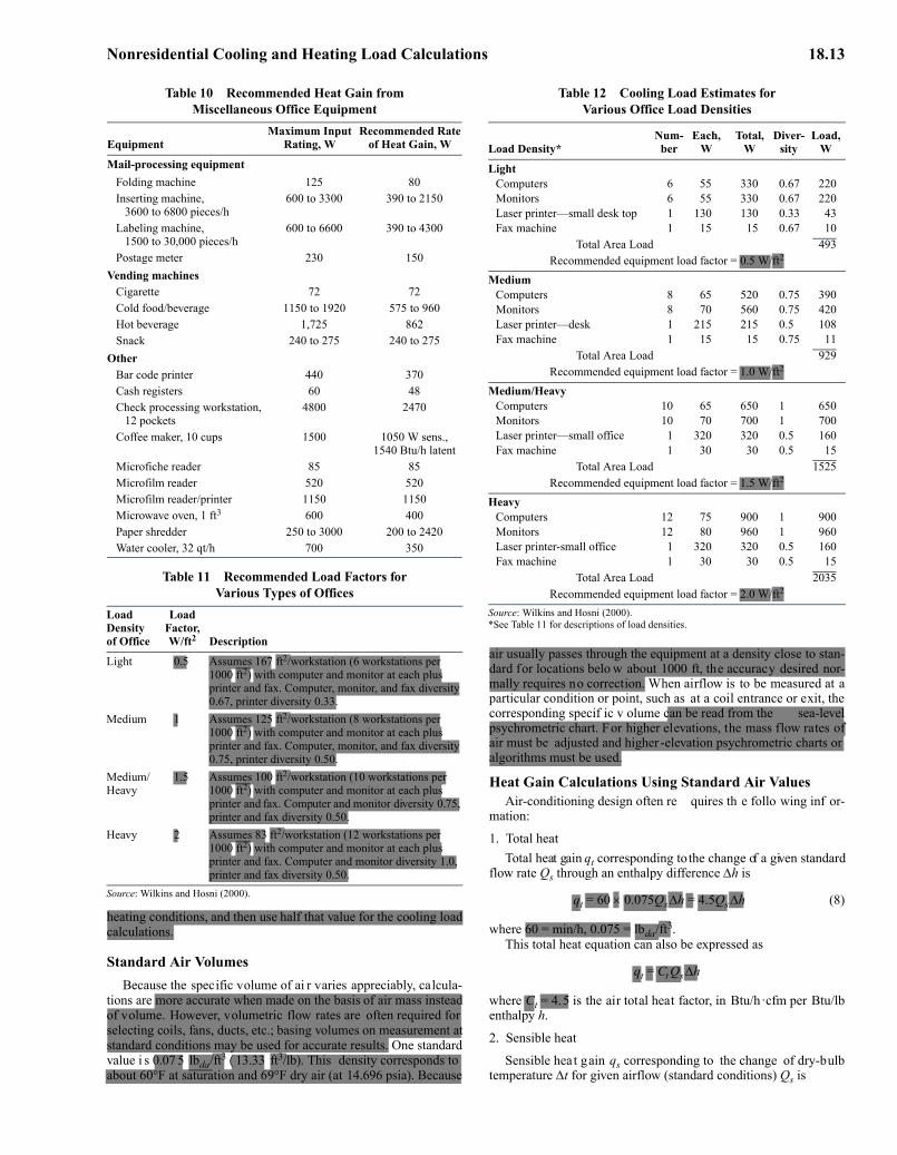
Miscellaneous Off ice Equipmen t. Table 10 presents data onmiscellaneous of fice equipment such as v ending machines andmailing equipment.

Diversity. The ratio of measured peak electrical load at equip-ment panels to the sum of the maximum electrical load of each indi-vidual item o f equipment is the usage diversity. A small, one- ortwo-person of fice containing eq uipment li sted in Tables 8 t o 10usually contributes heat gain to the space at the sum of the appro-priate l isted values. Progressively larger areas wi th many equip-ment items always experience some de gree of usa ge di versityresulting fr om whatever percenta ge of su ch eq uipment is n ot inoperation at any given time.

Wilkins a nd Mc Gaffin (1994) me asured di versity in 23 areaswithin five different buildings totaling o ver 275,000 ft2. Diversitywas found to range between 37 and 78%, with the average (normal-ized based on area) being 46%. Figure 4 illustrates the relationshipbetween nameplate, sum of peaks, a-nd actual electrical load withdiversity accounted for, based on the average of the total area tested.Data on actual diversity can be used as a guide, but diversity varies

Table 5B Recommended Rates of Radiant Heat Gain from Hooded Electric Appliances During Idle (Ready-to-Cook) Conditions

Appliance

Energy Rate, Btu/h Rate of Heat Gain, Btu/h

Usage Factor Fu Radiation Factor FrRated Standby Sensible Radiant

Broiler: underfired 3 ft 36,900 30,900 10,800 0.84 0.35Cheesemelter* 12,300 11,900 4,600 0.97 0.39Fryer: kettle 99,000 1,800 500 0.02 0.28Fryer: open deep-fat, 1-vat 47,800 2,800 1,000 0.06 0.36Fryer: pressure 46,100 2,700 500 0.06 0.19Griddle: double sided 3 ft (clamshell down)* 72,400 6,900 1,400 0.10 0.20Griddle: double sided 3 ft (clamshell up)* 72,400 11,500 3,600 0.16 0.31Griddle: flat 3 ft 58,400 11,500 4,500 0.20 0.39Griddle-small 3 ft* 30,700 6,100 2,700 0.20 0.44Induction cooktop* 71,700 0 0 0.00 0.00Induction wok* 11,900 0 0 0.00 0.00Oven: combi: combi-mode* 56,000 5,500 800 0.10 0.15Oven: combi: convection mode 56,000 5,500 1,400 0.10 0.25Oven: convection full-size 41,300 6,700 1,500 0.16 0.22Oven: convection half-size* 18,800 3,700 500 0.20 0.14Pasta cooker* 75,100 8,500 0 0.11 0.00Range top: top off/oven on* 16,600 4,000 1,000 0.24 0.25Range top: 3 elements on/oven off 51,200 15,400 6,300 0.30 0.41Range top: 6 elements on/oven off 51,200 33,200 13,900 0.65 0.42Range top: 6 elements on/oven on 67,800 36,400 14,500 0.54 0.40Range: hot-top 54,000 51,300 11,800 0.95 0.23Rotisserie* 37,900 13,800 4,500 0.36 0.33Salamander* 23,900 23,300 7,000 0.97 0.30Steam kettle: large (60 gal) simmer lid down* 110,600 2,600 100 0.02 0.04Steam kettle: small (40 gal) simmer lid down* 73,700 1,800 300 0.02 0.17Steamer: compartment: atmospheric* 33,400 15,300 200 0.46 0.01Tilting skillet/braising pan 32,900 5,300 0 0.16 0.00

Source: Swierczyna et al. (2008, 2009).

18.10 2009 ASHRAE Handbook—Fundamentals

significantly with occupanc y. The proper di versity f actor for anoffice of mail-o rder catalog telephone operators is dif ferent fromthat for an office of sales representatives who travel regularly.

ASHRAE research project R P-1093 derived diversity prof ilesfor use in energy calculations (Abushakra et al. 2004; Claridge et al.2004). Those prof iles were der ived from available measured datasets for a variety of office buildings, and indicated a range of peakweekday diversity factors for lighting ranging from 70 to 85% andfor receptacles (appliance load) between 42 and 89%.

Heat Gain per Unit Area. Wilkins and Hosni (2000) and Wilkinsand McGaffin (1994) summarized re search on a heat gain per unitarea basis. Diversity testing showed that the actual heat gain per unitarea, or load factor, ranged from 0.44 to 1.08 W/ft2, with an average

(normalized based on area) of 0.81 W/ft2. Spaces tested were fullyoccupied and highly automated, comprising 21 unique areas in fivebuildings, with a computer and monitor at every workstation. Table11 presents a range of load factors with a subjective description of thetype of space to which they would apply. Table 12 presents more spe-cific data that can be used to better quantify the amount of equipmentin a spa ce and e xpected load f actor. The medium load den sity islikely to be appropriate for most sta ndard of fice spaces.Medium/heavy or heavy load densities may be encountered but can

Table 5C Recommended Rates of Radiant Heat Gain from Hooded Gas Appliances During Idle (Ready-to-Cook) Conditions

Appliance

Energy Rate, Btu/h Rate of Heat Gain, Btu/h

Usage Factor Fu

Radiation Factor FrRated Standby Sensible Radiant

Broiler: batch* 95,000 69,200 8,100 0.73 0.12Broiler: chain (conveyor) 132,000 96,700 13,200 0.73 0.14Broiler: overfired (upright)* 100,000 87,900 2,500 0.88 0.03Broiler: underfired 3 ft 96,000 73,900 9,000 0.77 0.12Fryer: doughnut 44,000 12,400 2,900 0.28 0.23Fryer: open deep-fat, 1 vat 80,000 4,700 1,100 0.06 0.23Fryer: pressure 80,000 9,000 800 0.11 0.09Griddle: double sided 3 ft (clamshell down)* 108,200 8,000 1,800 0.07 0.23Griddle: double sided 3 ft (clamshell up)* 108,200 14,700 4,900 0.14 0.33Griddle: flat 3 ft 90,000 20,400 3,700 0.23 0.18Oven: combi: combi-mode* 75,700 6,000 400 0.08 0.07Oven: combi: convection mode 75,700 5,800 1,000 0.08 0.17Oven: convection full-size 44,000 11,900 1,000 0.27 0.08Oven: conveyor (pizza) 170,000 68,300 7,800 0.40 0.11Oven: deck 105,000 20,500 3,500 0.20 0.17Oven: rack mini-rotating* 56,300 4,500 1,100 0.08 0.24Pasta cooker* 80,000 23,700 0 0.30 0.00Range top: top off/oven on* 25,000 7,400 2,000 0.30 0.27Range top: 3 burners on/oven off 120,000 60,100 7,100 0.50 0.12Range top: 6 burners on/oven off 120,000 120,800 11,500 1.01 0.10Range top: 6 burners on/oven on 145,000 122,900 13,600 0.85 0.11Range: wok* 99,000 87,400 5,200 0.88 0.06Rethermalizer* 90,000 23,300 11,500 0.26 0.49Rice cooker* 35,000 500 300 0.01 0.60Salamander* 35,000 33,300 5,300 0.95 0.16Steam kettle: large (60 gal) simmer lid down* 145,000 5,400 0 0.04 0.00Steam kettle: small (10 gal) simmer lid down* 52,000 3,300 300 0.06 0.09Steam kettle: small (40 gal) simmer lid down 100,000 4,300 0 0.04 0.00Steamer: compartment: atmospheric * 26,000 8,300 0 0.32 0.00Tilting skillet/braising pan 104,000 10,400 400 0.10 0.04

Source: Swierczyna et al. (2008, 2009).

Table 5D Recommended Rates of Radiant Heat Gain from Hooded Solid Fuel Appliances During Idle (Ready-to-Cook)

Conditions

Energy Rate, Btu/h

Rate of Heat Gain, Btu/h Usage

Factor Fu

Radiation Factor FrAppliance Rated Standby Sensible

Broiler: solid fuel: charcoal

40 lb 42,000 6200 N/A 0.15

Broiler: solid fuel: wood (mesquite)*

40 lb 49,600 7000 N/A 0.14

Source: Swierczyna et al. (2008, 2009).

Fig. 4 Office Equipment Load Factor Comparison

Fig. 4 Office Equipment Load Factor Comparison(Wilkins and McGaffin 1994)

Nonresidential Cooling and Heating Load Calculations 18.11

be c onsidered e xtremely conserv ative e stimates e ven for de nselypopulated and highly automated spaces.

Radiant Convective Split. ASHRAE research project RP-1482(Hosni and Beck 2008) is examining the radiant/convective split forcommon office equipment; the most important differentiating fea-ture is whether the equipment had a cooling fan. Footnotes in Tables8 and 9 summarizes those results.

INFILTRATION AND MOISTURE MIGRATION HEAT GAINS

Two other load components contribute to space cooling loaddirectly without time delay from building mass: (1) infiltration, and(2) moisture migration through the building envelope.

INFILTRATIONPrinciples of estimating infiltration in buildings, with emphasis

on the heating season, are discussed in Chapter 16. When econom-ically feasible, somewhat more outdoor air should be introducedto a building than the total of that exhausted, to create a slight over-all positive pressure in the building relative to the outdoors. Under

these condit ions, air us ually e xfiltrates, rather than infiltrates,through the building envelope and thus effectively eliminates infil-tration sensible and latent heat gains. However, there is concern,especially in some climates, th at water may condense within thebuilding envelope; actively managing space air pressures to reducethis condensation problem, as well as infiltration, may be needed.

When posit ive air pre ssure is assumed, most designers d o notinclude inf iltration in cooling load calcula tions for commerci albuildings. However, including some infiltration for spaces such entryareas or lo ading docks may be appropriate, especially when thosespaces are on the windw ard side of b uildings. But the do wnwardstack effect, as occurs when indoor air is denser than the outdoor,

Table 5E Recommended Rates of Radiant and Convective Heat Gain from Warewashing Equipment During Idle (Standby) or Washing Conditions

Appliance

Energy Rate, Btu/h

Rate of Heat Gain, Btu/h

Usage Factor Fu

Radiation Factor Fr

Unhooded Hooded

RatedStandby/ Washing

Sensible Radiant

Sensible Convective Latent Total

Sensible Radiant

Dishwasher (conveyor type, chemical sanitizing)

46,800 5700/43,600 0 4450 13490 17940 0 0.36 0

Dishwasher (conveyor type, hot-water sanitizing) standby

46,800 5700/N/A 0 4750 16970 21720 0 N/A 0

Dishwasher (door-type, chemical sanitizing) washing

18,400 1200/13,300 0 1980 2790 4770 0 0.26 0

Dishwasher (door-type, hot-water sanitizing) washing

18,400 1200/13,300 0 1980 2790 4770 0 0.26 0

Dishwasher* (under-counter type, chemical sanitizing) standby

26,600 1200/18,700 0 2280 4170 6450 0 0.35 0.00

Dishwasher* (under-counter type, hot-water sanitizing) standby

26,600 1700/19,700 800 1040 3010 4850 800 0.27 0.34

Booster heater* 130,000 0 500 0 0 0 500 0 N/A

Note: Heat load values are prorated for 30% washing and 70% standby. Source: Swierczyna et al. (2008, 2009).

Table 6 Recommended Heat Gain from Typical Medical Equipment

Equipment Nameplate, W Peak, W Average, W

Anesthesia system 250 177 166Blanket warmer 500 504 221Blood pressure meter 180 33 29Blood warmer 360 204 114ECG/RESP 1440 54 50Electrosurgery 1000 147 109Endoscope 1688 605 596Harmonical scalpel 230 60 59Hysteroscopic pump 180 35 34Laser sonics 1200 256 229Optical microscope 330 65 63Pulse oximeter 72 21 20Stress treadmill N/A 198 173Ultrasound system 1800 1063 1050Vacuum suction 621 337 302X-ray system 968 82

1725 534 4802070 18

Source: Hosni et al. (1999).

Table 7 Recommended Heat Gain from Typical Laboratory Equipment

Equipment Nameplate, W Peak, W Average, WAnalytical balance 7 7 7Centrifuge 138 89 87

288 136 1325500 1176 730

Electrochemical analyzer 50 45 44100 85 84

Flame photometer 180 107 105Fluorescent microscope 150 144 143

200 205 178Function generator 58 29 29Incubator 515 461 451

600 479 2643125 1335 1222

Orbital shaker 100 16 16Oscilloscope 72 38 38

345 99 97Rotary evaporator 75 74 73

94 29 28Spectronics 36 31 31Spectrophotometer 575 106 104

200 122 121N/A 127 125

Spectro fluorometer 340 405 395Thermocycler 1840 965 641

N/A 233 198Tissue culture 475 132 46

2346 1178 1146Source: Hosni et al. (1999).

18.12 2009 ASHRAE Handbook—Fundamentals

might eliminate infiltration to the se entries on lo wer floors of tallbuildings; infiltration may occur on the upper floors during coolingconditions if makeup air is not sufficient.

Infiltration also depends on wind direction and magnitude, tem-perature dif ferences, construction type and quality, and occupant

use of exterior doors and operable windows. As such, it is impossi-ble to accurately predict infiltration rates. Designers usually predictoverall rates of infiltration using the number of air changes perhour (ach). A common guideline for climates and buildings typicalof at least the central United States is to estimate the achs for winter

Table 8 Recommended Heat Gain from Typical Computer Equipment

Equipment DescriptionNameplate Power Consumption, W

Average Power Consumption, W

Desktop computera Manufacturer A (model A); 2.8 GHz processor, 1 GB RAM 480 73Manufacturer A (model B); 2.6 GHz processor, 2 GB RAM 480 49Manufacturer B (model A); 3.0 GHz processor, 2 GB RAM 690 77Manufacturer B (model B); 3.0 GHz processor, 2 GB RAM 690 48Manufacturer A (model C); 2.3 GHz processor, 3 GB RAM 1200 97

Laptop computerb Manufacturer 1; 2.0 GHz processor, 2 GB RAM, 17 in. screen 130 36Manufacturer 1; 1.8 GHz processor, 1 GB RAM, 17 in. screen 90 23Manufacturer 1; 2.0 GHz processor, 2 GB RAM, 14 in. screen 90 31Manufacturer 2; 2.13 GHz processor, 1 GB RAM, 14 in. screen, tablet PC

90 29

Manufacturer 2; 366 MHz processor, 130 MB RAM, 14 in. screen) 70 22Manufacturer 3; 900 MHz processor, 256 MB RAM (10.5 in. screen) 50 12

Flat-panel monitorc Manufacturer X (model A); 30 in. screen 383 90Manufacturer X (model B); 22 in. screen 360 36Manufacturer Y (model A), 19 in. screen 288 28Manufacturer Y (model B), 17 in. screen 240 27Manufacturer Z (model A), 17 in. screen 240 29Manufacturer Z (model C), 15 in. screen 240 19

Source: Hosni and Beck (2008).aPower consumption for newer desktop computers in operational mode varies from 50 to 100 W, but a con-servative value of about 65 W may be used. Power consumption in sleep mode is negligible. Because ofcooling fan, approximately 90% of load is by convection and 10% is by radiation. Actual power consump-tion is about 10 to 15% of nameplate value.

bPower consumption of laptop computers is relatively small: depending on processor speed and screen size,it varies from about 15 to 40 W. Thus, differentiating between radiative and convective parts of the coolingload is unnecessary and the entire load may be classified as convective. Otherwise, a 75/25% split betweenconvective and radiative components may be used. Actual power consumption for laptops is about 25% ofnameplate values.

cFlat-panel monitors have replaced cathode ray tube (CRT) moni-tors in many w orkplaces, providing bet ter resolution and b eingmuch lighter. Power consumption depends on size and resolution,and ranges from about 20 W (for 15 in. size) to 90 W (for 30 in.).The mos t com mon s izes in w orkplaces are 19 and 22 in., forwhich an average 30 W p ower consumption value may b e used.Use 60/40% split between co nvective and radiative components.In idle mod e, m onitors ha ve ne gligible po wer consumption.Nameplate values should not be used.

Table 9 Recommended Heat Gain from Typical Laser Printers and Copiers

Equipment Description Nameplate Power Consumption, W Average Power Consumption, W

Laser printer, typical desktop, small-office typea

Printing speed up to 10 pages per minute 430 137Printing speed up to 35 pages per minute 890 74Printing speed up to 19 pages per minute 508 88Printing speed up to 17 pages per minute 508 98Printing speed up to 19 pages per minute 635 110Printing speed up to 24 page per minute 1344 130

Multifunction (copy, print, scan)b

Small, desktop type 600 30

40 15Medium, desktop type 700 135

Scannerb Small, desktop type 19 16Copy machinec Large, multiuser, office type 1750 800 (idle 260 W)

1440 550 (idle 135 W)1850 1060 (idle 305 W)

Fax machine Medium 936 90Small 40 20

Plotter Manufacturer A 400 250Manufacturer B 456 140

Source: Hosni and Beck (2008).aVarious laser printers commercially available and commonly used in personal offices were tested for power consumption in print mode, which varied from 75 to 140 W, depending on model, print capacity, and speed. Average power con-sumption of 110 W may be used. Split between convection and radiation is approximately 70/30%.

bSmall multifunction (copy, scan, print) systems use about 15 to 30 W; medium-sized ones use about 135 W. Power consumption in idle mode is negligible.

Nameplate values do not represent actual power consumption and should not be used. Small, single-sheet scanners consume less than 20 W and do not contribute significantly to building cooling load.

cPower consumption for large copy machines in large offices and copy centers ranges from about 550 to 1100 W in copy mode. Consumption in idle mode varies from about 130 to 300 W. Count idle-mode power consumption as mostly convective in cooling load calcu-lations.

Nonresidential Cooling and Heating Load Calculations 18.13

heating conditions, and then use half that value for the cooling loadcalculations.

Standard Air VolumesBecause the specific volume of ai r varies appreciably, calcula-

tions are more accurate when made on the basis of air mass insteadof volume. However, volumetric flow rates are often required forselecting coils, fans, ducts, etc.; basing volumes on measurement atstandard conditions may be used for accurate results. One standardvalue i s 0.07 5 lbda/ft3 ( 13.33 ft3/lb). This density corresponds toabout 60°F at saturation and 69°F dry air (at 14.696 psia). Because

air usually passes through the equipment at a density close to stan-dard for locations belo w about 1000 ft, the accuracy desired nor-mally requires no correction. When airflow is to be measured at aparticular condition or point, such as at a coil entrance or exit, thecorresponding specif ic v olume can be read from the sea-levelpsychrometric chart. For higher elevations, the mass flow rates ofair must be adjusted and higher -elevation psychrometric charts oralgorithms must be used.

Heat Gain Calculations Using Standard Air ValuesAir-conditioning design often re quires th e follo wing inf or-

mation:

1. Total heatTotal heat gain qt corresponding to the change of a given standard

flow rate Qs through an enthalpy difference Δh is

qt = 60 × 0.075Qs Δh = 4.5Qs Δh (8)

where 60 = min/h, 0.075 = lbda/ft3.This total heat equation can also be expressed as

qt = Ct Qs Δh

where Ct = 4.5 is the air total heat factor, in Btu/h·cfm per Btu/lbenthalpy h.

2. Sensible heat

Sensible heat gain qs corresponding to the change of dry-bulbtemperature Δt for given airflow (standard conditions) Qs is

Table 10 Recommended Heat Gain from Miscellaneous Office Equipment

EquipmentMaximum Input

Rating, WRecommended Rate

of Heat Gain, W

Mail-processing equipmentFolding machine 125 80Inserting machine,

3600 to 6800 pieces/h600 to 3300 390 to 2150

Labeling machine,1500 to 30,000 pieces/h

600 to 6600 390 to 4300

Postage meter 230 150Vending machines

Cigarette 72 72Cold food/beverage 1150 to 1920 575 to 960Hot beverage 1,725 862Snack 240 to 275 240 to 275

OtherBar code printer 440 370Cash registers 60 48Check processing workstation,

12 pockets4800 2470

Coffee maker, 10 cups 1500 1050 W sens., 1540 Btu/h latent

Microfiche reader 85 85Microfilm reader 520 520Microfilm reader/printer 1150 1150Microwave oven, 1 ft3 600 400Paper shredder 250 to 3000 200 to 2420Water cooler, 32 qt/h 700 350

Table 11 Recommended Load Factors for Various Types of Offices

Load Density of Office

Load Factor, W/ft2 Description

Light 0.5 Assumes 167 ft2/workstation (6 workstations per 1000 ft2) with computer and monitor at each plus printer and fax. Computer, monitor, and fax diversity 0.67, printer diversity 0.33.

Medium 1 Assumes 125 ft2/workstation (8 workstations per 1000 ft2) with computer and monitor at each plus printer and fax. Computer, monitor, and fax diversity 0.75, printer diversity 0.50.

Medium/ Heavy

1.5 Assumes 100 ft2/workstation (10 workstations per 1000 ft2) with computer and monitor at each plus printer and fax. Computer and monitor diversity 0.75, printer and fax diversity 0.50.

Heavy 2 Assumes 83 ft2/workstation (12 workstations per 1000 ft2) with computer and monitor at each plus printer and fax. Computer and monitor diversity 1.0, printer and fax diversity 0.50.

Source: Wilkins and Hosni (2000).

Table 12 Cooling Load Estimates for Various Office Load Densities

Num-ber

Each,W

Total,W

Diver-sity

Load, WLoad Density*

LightComputers 6 55 330 0.67 220Monitors 6 55 330 0.67 220Laser printer—small desk top 1 130 130 0.33 43Fax machine 1 15 15 0.67 10

Total Area Load 493Recommended equipment load factor = 0.5 W/ft2

MediumComputers 8 65 520 0.75 390Monitors 8 70 560 0.75 420Laser printer—desk 1 215 215 0.5 108Fax machine 1 15 15 0.75 11

Total Area Load 929Recommended equipment load factor = 1.0 W/ft2

Medium/HeavyComputers 10 65 650 1 650Monitors 10 70 700 1 700Laser printer—small office 1 320 320 0.5 160Fax machine 1 30 30 0.5 15

Total Area Load 1525Recommended equipment load factor = 1.5 W/ft2

HeavyComputers 12 75 900 1 900Monitors 12 80 960 1 960Laser printer-small office 1 320 320 0.5 160Fax machine 1 30 30 0.5 15

Total Area Load 2035Recommended equipment load factor = 2.0 W/ft2

Source: Wilkins and Hosni (2000).*See Table 11 for descriptions of load densities.

18.14 2009 ASHRAE Handbook—Fundamentals

qs = 60 × 0.075(0.24 + 0.45W )Qs Δt (9)

where0.24 = specific heat of dry air, Btu/lb·°F

W = humidity ratio, lbw/lbda0.45 = specific heat of water vapor, Btu/lb·°F

The specif ic heats are fo r a r ange from ab out –100 to 2 00°F.When W = 0, the value of 60 × 0.075 (0.24 + 0.45W) = 1.08; whenW = 0.01, the value is 1.10; when W = 0.02, the value is 1.12; andwhen W = 0.03, the v alue is 1.14 . Because a v alue of W = 0.01approximates conditions found in many air-conditioning problems,the sensible heat change (in Btu/h) has traditionally been found as

qs = 1.10Qs Δt (10)

This sensible heat equation can also be expressed as

qs = Cs Qs Δt

where Cs = 1.1 is the air sensible heat factor, in Btu/h·cfm·°F.

3. Latent heat

Latent heat gain ql corresponding to the change of humidity ratioΔW (in lbm,w/lbm,da) for given airflow (standard conditions) Qs is

ql = 60 × 0.075 × 1076Qs ΔW = 4840Qs ΔW (11)

where 1076 Btu/lb is the approximate heat content of 50% rh vaporat 75°F less the heat content of water at 50°F. A common designcondition for the space is 50% rh at 75°F, and 50°F is normal con-densate temperature from cooling and dehumidifying coils.

This latent heat equation can also be expressed as

ql = Cl Qs ΔW

where Cl = 4840 is the air latent heat factor, in Btu/h·cfm. When ΔWis in grw /lbm,da, Cl = 0.69 Btu/h·cfm.

4. Altitude correction for total, sensible, and latent heat equations

The constants 4.5, 1.10, and 4840 are useful in air-conditioningcalculations at sea level (14.696 psia) and for normal temperaturesand moist ure ra tios. For ot her con ditions, mor e prec ise v aluesshould be used. For an altitude of 5000 ft ( 12.2 psia), appropriatevalues are 3.74, 0.92, and 402 7. Equations (9) to (11) can be cor-rected for altitudes other than sea level by multiplying them by theratio of pressure at sea level divided by the pressure at actual alti-tude. This can be derived from Equation (3) in Chapter 1 as

Cx,alt = Cx,0P/P0

where Cx,0 is any of the sea-level C values and P/P0 = [1 – elevation× (6.8754 × 10–6)]5.2559, where elevation is in feet.

LATENT HEAT GAIN FROM MOISTURE DIFFUSION

Diffusion of moisture through building materials is a natural phe-nomenon that is always present. Chapters 25 to 27 cover principles,materials, and specific methods used to control moisture. Moisturetransfer through walls and roofs is of ten neglected in comfo rt airconditioning because the actual rate is quite small and the corre-sponding latent heat g ain is insignificant. Permea bility and per-meance values for various building materials are given in Chapter26. Vapor retarders should be specified and installed in the properlocation to keep moisture transfer to a minimum, and to minimizecondensation within the en velope. Moisture migration up throughslabs-on-grade and basement floors has been found to be signif i-cant, but has historically not been addressed in cooling load calcu-lations. Under-slab continuous moisture retarders and drainage canreduce upward moisture flow.

Some industrial applications require low moisture to be main-tained in a con ditioned space. In the se cases, the latent heat gainaccompanying moisture transfer through walls and roofs may begreater than any other latent heat gain. This gain is computed by

(12)

where= latent heat gain from moisture transfer, Btu/h

M = permeance of wall or roof assembly, perms or grains/(ft2·h·in. Hg)

7000 = grains/lbA = area of wall or roof surface, ft2

Δpv = vapor pressure difference, in. Hghg = enthalpy at room conditions, Btu/lbhf = enthalpy of water condensed at cooling coil, Btu/lb

hg – hf = 1076 Btu/lb when room temperature is 75°F and condensate off coil is 50°F

OTHER LATENT LOADSMoisture sources within a b uilding (e .g., shower areas, swim-

ming pools or natatoriums, arboretums) can also contribute to latentload. Unlike sensible loads, which correlate to supply air quantitiesrequired in a space, latent loads usually only affect cooling coils siz-ing or refrigeration load. Because air from showers and some othermoisture-generating areas is exhausted completely, those airbornelatent loads do not reach the cooling coil and thus do not contributeto cooling load. However, system loads associated with ventilationair required to mak e up e xhaust ai r must be recognized, and an yrecirculated air’s moisture must be consid ered when sizing thedehumidification equipment.

For natatoriums, occupant comfort and humidity control are crit-ical. In many instances, size, location, and environmental require-ments make complete exhaust systems expensive and in effective.Where recirculating mechanical cooling systems are used, evapora-tion (latent) loads are significant. Chapter 4 of the 2007 ASHRAEHandbook—HVAC Applications provides guidance on natatoriumload calculations.

FENESTRATION HEAT GAINFor spaces with neutral or positive air pressurization, the primary

weather-related variable affecting cooling load is solar rad iation.The effect of solar radiation is more pronounced and immediate onexposed, nonopaque surfaces. Chapter 14 includes procedures forcalculating clear-sky solar radiation intensity and incidence anglesfor weather conditions encountered at specific locations. That chap-ter also includes some useful solar equations. Calculation of solarheat gain and conductive h eat tr ansfer throu gh v arious glazingmaterials and associated mounting frames, with or without interiorand/or exterior shading devices, is discussed in Chap ter 15. Thischapter covers application of such data to overall heat gain evalua-tion, and conversion of calculated heat gain into a composite cool-ing load for the conditioned space.

FENESTRATION DIRECT SOLAR, DIFFUSE SOLAR, AND CONDUCTIVE HEAT GAINS

For fenestration heat gain, use the following equations:Direct beam solar heat gain qb:

qb = AEt,b SHGC(θ)IAC(θ,Ω) (13)

Diffuse solar heat gain qd:

qd = A(Et,d + Et,r)⟨SHGC⟩D IACD (14)

Conductive heat gain qc:

qc = UA(Tout – Tin) ( 15)

ql mM/7000( )A pvΔ hg hf–( )=

ql m

Nonresidential Cooling and Heating Load Calculations 18.15 Total fenestration heat gain Q:

Q = qb + qd + qc (16)

whereA = window area, ft2

Et,b, Et,d,and Et,r = beam, sky diffuse, and ground-reflected diffuse irradiance,

calculated using equations in Chapter 14SHGC(θ) = beam solar heat gain coefficient as a function of

incident angle θ; may be interpolated between values in Table 10 of Chapter 15

⟨SHGC⟩D = diffuse solar heat gain coefficient (also referred to as hemispherical SHGC); from Table 10 of Chapter 15

Tin = inside temperature, °FTout = outside temperature, °F

U = overall U-factor, including frame and mounting orientation from Table 4 of Chapter 15, Btu/h·ft2·°F

IAC(θ.Ω) = indoor solar attenuation coefficient for beam solar heat gain coefficient; = 1.0 if no inside shading device. IAC(θ.Ω) is a function of shade type and, depending on type, may also be a function of beam solar angle of incidence θ and shade geometry

IACD = indoor solar attenuation coefficient for diffuse solar heat gain coefficient; = 1.0 if not inside shading device. IACD is a function of shade type and, depending on type, may also be a function of shade geometry

If specific window manufacturer’s SHGC and U-factor data areavailable, those sh ould be used . F or fenestration eq uipped withinside shading (blinds, drapes, or shades), the indoor solar attenua-tion coefficients IAC(θ.Ω) and IACD are listed in Tables 13A to 13Gof Chapter 15.

Note that, as discussed in Chapter 15, fenestration ratings (U-factor and SHGC) are b ased on the entire prod uct area, includingframes. Thus, for load calculations, fenestration area is the area ofthe entire opening in the wall or roof.

EXTERIOR SHADINGNonuniform e xterior shading, ca used b y ro of o verhangs, sid e

fins, or building projections, re quires separate hourly calcu lationsfor the externally shaded and unshaded areas of the window in ques-tion, with the inside shading SHGC still used to account for an yinternal shading devices. The areas, shaded and unshaded, dependon the location of the shadow line on a surface in the plane of theglass. Sun (1968) developed fundamental algorithms for analysis ofshade p atterns. McQuiston and Spitler ( 1992) p rovide g raphicaldata to facilitate shadow line calculation.

Equations for calculating shade angles [Chapter 15, Equations(39) to (42)] can be used to determine the shape and area of a mov-ing shadow falling across a gi ven window from external shadingelements during the course of a design day. Thus, a sub profile ofheat gain for that window can be created by separating its sunlit andshaded areas for each hour.

HEAT BALANCE METHODCooling load estimation involves calculating a surface-by-surface

conductive, convective, and radiative heat balance for each room sur-face and a convective heat balance for the room air. These principlesform the fou ndation for all methods described in this chapter. Theheat balance (HB) method solves the problem directly instead of in-troducing transformation-based procedures. The advantages are thatit contains no arbitrarily set parameters, and no processes are hiddenfrom view.

Some computations required by this rigorous approach requirethe use of computers. The heat balance procedure is not new. Manyenergy calculation programs have used it in some form for manyyears. The first implementation that incorporated all the elements to

form a complete method w as NBSLD (K usuda 1967). The h eatbalance procedur e is also impl emented i n both t he BLAS T andTARP energy analysis programs (Walton 1983). Before ASHRAEresearch project RP-875, the method had never been described com-pletely o r in a fo rm applicable to cooling load calcu lations. Thepapers resulting from RP-875 describe the heat balance procedurein detail (Liesen and Pedersen 1997; McClellan and Pedersen 1997;Pedersen et al. 1997).

The HB method is codified in the software called Hbfort thataccompanies C ooling and Heating Load Calculation Principles(Pedersen et al. 1998).

ASHRAE re search proj ect RP -1117 con structed tw o modelrooms for which coo ling lo ads we re ph ysically measured u singextensive instrumentation (Chantrasrisalai et al. 2003; Eldridge etal. 2003; Iu et al. 2003). HB calculations closely approximated mea-sured cooling loads when pro vided with detailed data for the testrooms.

ASSUMPTIONSAll calculation procedures involve some kind of model; all mod-

els require simplifyi ng assumptions and, ther efore, are approxi-mate. The most fundamental assumption is that air in the thermalzone can be modeled as well mixed, meaning its temperature is uni-form througho ut the zone. ASHRAE research project RP- 664(Fisher and Pedersen 1997) established that this assumption is validover a wide range of conditions.

The ne xt ma jor a ssumption is t hat the su rfaces of the room(walls, windows, floor, etc.) can be treated as having

• Uniform surface temperatures• Uniform long-wave (LW) and short-wave (SW) irradiation• Diffuse radiating surfaces• One-dimensional heat conduction within

The re sulting formul ation is ca lled t he heat balan ce (HB)model. Note that the assumptions, although common, are quiterestrictive and set ce rtain l imits on the inform ation th at c an beobtained from the model.

ELEMENTSWithin the framework of the assumptions, the HB can be viewed

as four distinct processes:

1. Outside-face heat balance2. Wall conduction process3. Inside-face heat balance4. Air heat balance

Figure 5 shows the relationship between these processes for asingle opaque surface. The top part of the figure, inside the shadedbox, is repeated for each surface enclosing the zone. The process fortransparent surfaces is similar, but the absorbed solar componentappears in the conduction process block instead of at the outsideface, and the absorbed component splits into inward- and outward-flowing fractions. These components participate in the surface heatbalances.

Outside-Face Heat BalanceThe heat balance on the outside face of each surface is

(17)

whereq″αsol = absorbed direct and diffuse solar radiation flux (q/A), Btu/h·ft2q″LWR = net long-wave radiation flux exchange with air and

surroundings, Btu/h·ft2q″conv = convective exchange flux with outside air, Btu/h·ft2

q″ko = conductive flux (q/A) into wall, Btu/h·ft2

q″αsol q″LWR q″conv q″ko–+ + 0=

18.16 2009 ASHRAE Handbook—Fundamentals

All terms are positive for net flux to the face except q″ko, which istraditionally taken to be positive from outside to inside the wall.

Each term in Equation (17) has been modeled in several ways,and in simplif ied methods the f irst thr ee terms are combined byusing the sol-air temperature.

Wall Conduction ProcessThe wall conduction process has been formulated in more ways

than any of the other processes. Techniques include

• Numerical finite difference• Numerical finite element• Transform methods• Time series methods

This process introduces part of the time dependence inherent inload calculation. Figure 6 shows surface temperatures on the insideand outside faces of the wall element, and corresponding conductiveheat fluxes away from the outside face and toward the inside face.All four quantities are functions of time. Direct formulation of theprocess uses temperatur e functions as input o r known quantities,and heat fluxes as outputs or resultant quantities.

In some models, surface heat transfer coefficients are included aspart of the w all element, making the temperatures in question theinside and outside air temperatures. This is not a desirable formula-tion, because it hides the h eat transfer c oefficients and prohibi tschanging them as airflow conditions change. It also prohibits treat-ing the internal long-wave radiation exchange appropriately.

Because heat balances on both sides of the element induce boththe temperature and heat flux, the solution must deal with this simul-taneous condition. Two computational methods that have been usedwidely are finite difference and conduction transfer function meth-ods. Because of the computational time advantage, the conduction

transfer function fo rmulation ha s b een selected for pr esentationhere.

Inside-Face Heat BalanceThe heart of the HB method is the internal heat balance involving

the inside faces of the zone surfaces. This heat balance has manyheat transfer components, and they are all coupled. Both long-wave(LW) and short-wave (SW) radiation are important, as well as wallconduction and convection to the air. The inside face heat balancefor each surface can be written as follows:

q″LWX + q″SW + q″LWS + q″ki + q″sol + q″conv = 0 (18)

whereq″LWX = net long-wave radiant flux exchange between zone surfaces,

Btu/h·ft2q″SW = net short-wave radiation flux to surface from lights, Btu/h·ft2

q″LWS = long-wave radiation flux from equipment in zone, Btu/h·ft2q″ki = conductive flux through wall, Btu/h·ft2

q″sol = transmitted solar radiative flux absorbed at surface, Btu/h·ft2q″conv = convective heat flux to zone air, Btu/h·ft2

These terms are explained in the following paragraphs.LW Radiation Exchange Among Zone Surfaces. The limiting

cases for modeling internal LW radiation exchange are

• Zone air is completely transparent to LW radiation• Zone air completely absorbs LW radiation from surfaces in the zone

Most HB models treat air as completely transparent and not par-ticipating in LW radiation exchange among surfaces in the zone. Thesecond model is attractive because it can be formulated simply usinga combined radia tive and convective heat transfer coefficient fromeach surface to the zone air and thus dec ouples radiant e xchangeamong surfaces in the zone. Ho wever, because the transparent airmodel allows radiant e xchange a nd is m ore realistic, the secondmodel is inferior.

Furniture in a zone increases the amount of surface area that canparticipate in radiative and convective heat exchanges. It also addsthermal mass to the zone. These two changes can affect the timeresponse of the zone cooling load.

SW Radiation fr om Lights. Th e short-w avelength radiationfrom lights is usually assumed to be distributed over the surfaces inthe zone in some manner. The HB procedure retains this approachbut allows the distribution function to be changed.

LW Radiation from Internal Sources. The traditional modelfor this source def ines a radiati ve/convective split for he at int ro-duced into a zone from equipment. The radiative part is then distrib-uted over the zone’s surfaces in some manner. This model is no tcompletely realistic, and it departs from HB principles. In a true HB

Fig. 5 Schematic of Heat Balance Processes in a Zone

Fig. 5 Schematic of Heat Balance Processes in Zone

Fig. 6 Schematic of Wall Conduction Process

Fig. 6 Schematic of Wall Conduction Process

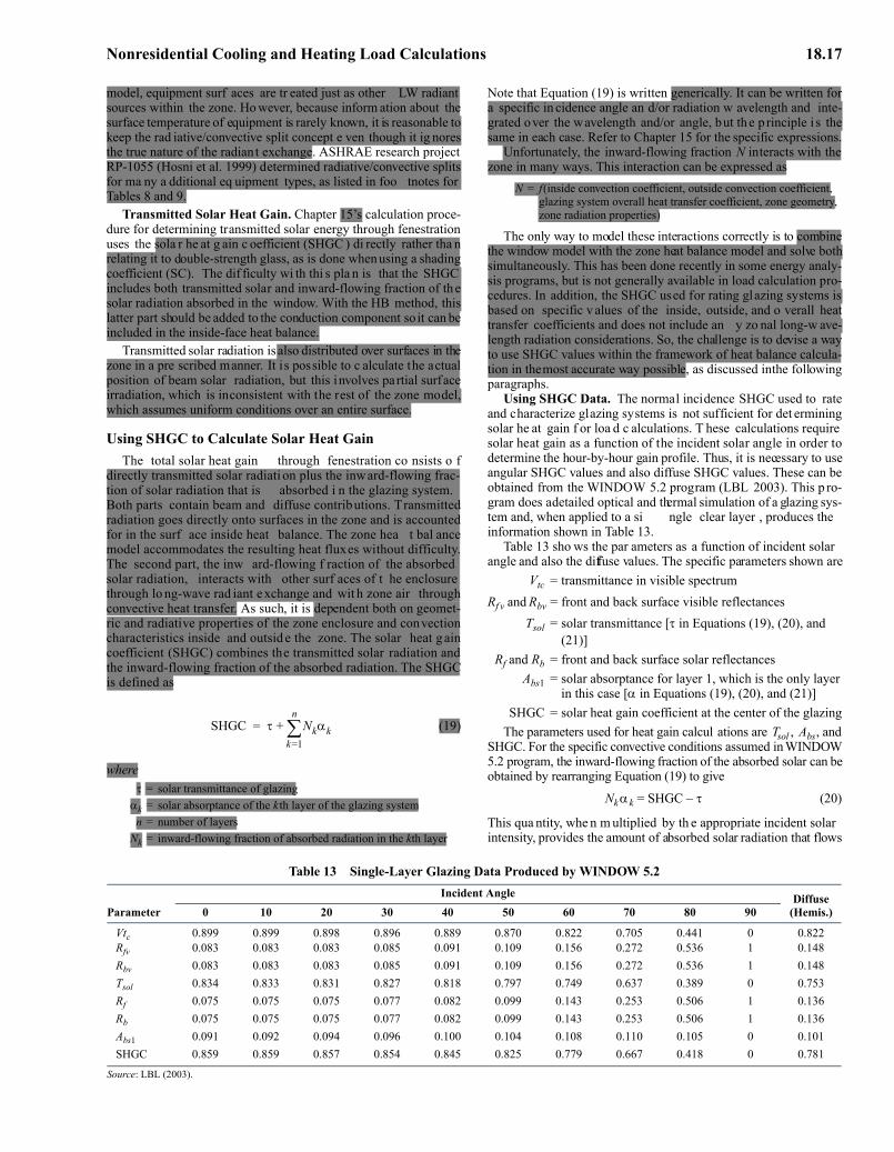
Nonresidential Cooling and Heating Load Calculations 18.17

model, equipment surf aces are tr eated just as other LW radiantsources within the zone. Ho wever, because inform ation about thesurface temperature of equipment is rarely known, it is reasonable tokeep the rad iative/convective split concept e ven though it ig noresthe true nature of the radiant exchange. ASHRAE research projectRP-1055 (Hosni et al. 1999) determined radiative/convective splitsfor ma ny a dditional eq uipment types, as listed in foo tnotes forTables 8 and 9.

Transmitted Solar Heat Gain. Chapter 15’s calculation proce-dure for determining transmitted solar energy through fenestrationuses the sola r he at g ain c oefficient (SHGC ) di rectly rather tha nrelating it to double-strength glass, as is done when using a shadingcoefficient (SC). The dif ficulty wi th thi s pla n is that the SHGCincludes both transmitted solar and inward-flowing fraction of thesolar radiation absorbed in the window. With the HB method, thislatter part should be added to the conduction component so it can beincluded in the inside-face heat balance.

Transmitted solar radiation is also distributed over surfaces in thezone in a pre scribed manner. It is possible to c alculate the actualposition of beam solar radiation, but this involves partial surfaceirradiation, which is inconsistent with the rest of the zone model,which assumes uniform conditions over an entire surface.

Using SHGC to Calculate Solar Heat GainThe total solar heat gain through fenestration co nsists o f

directly transmitted solar radiati on plus the inward-flowing frac-tion of solar radiation that is absorbed i n the glazing system.Both parts contain beam and diffuse contributions. Transmittedradiation goes directly onto surfaces in the zone and is accountedfor in the surf ace inside heat balance. The zone hea t bal ancemodel accommodates the resulting heat fluxes without difficulty.The second part, the inw ard-flowing f raction of the absorbedsolar radiation, interacts with other surf aces of t he enclosurethrough lo ng-wave rad iant exchange and wit h zone air throughconvective heat transfer. As such, it is dependent both on geomet-ric and radiative properties of the zone enclosure and convectioncharacteristics inside and outsid e the zone. The solar heat g aincoefficient (SHGC) combines the transmitted solar radiation andthe inward-flowing fraction of the absorbed radiation. The SHGCis defined as

(19)

whereτ = solar transmittance of glazing

αk = solar absorptance of the kth layer of the glazing systemn = number of layers

Nk = inward-flowing fraction of absorbed radiation in the kth layer

Note that Equation (19) is written generically. It can be written fora specific in cidence angle an d/or radiation w avelength and inte-grated over the wavelength and/or angle, but the p rinciple i s thesame in each case. Refer to Chapter 15 for the specific expressions.

Unfortunately, the inward-flowing fraction N interacts with thezone in many ways. This interaction can be expressed as

N = f(inside convection coefficient, outside convection coefficient, glazing system overall heat transfer coefficient, zone geometry, zone radiation properties)

The only way to model these interactions correctly is to combinethe window model with the zone heat balance model and solve bothsimultaneously. This has been done recently in some energy analy-sis programs, but is not generally available in load calculation pro-cedures. In addition, the SHGC used for rating glazing systems isbased on specific v alues of the inside, outside, and o verall heattransfer coefficients and does not include an y zo nal long-w ave-length radiation considerations. So, the challenge is to devise a wayto use SHGC values within the framework of heat balance calcula-tion in the most accurate way possible, as discussed in the followingparagraphs.

Using SHGC Data. The normal incidence SHGC used to rateand characterize glazing systems is not sufficient for det erminingsolar he at gain f or loa d c alculations. T hese calculations requiresolar heat gain as a function of the incident solar angle in order todetermine the hour-by-hour gain profile. Thus, it is necessary to useangular SHGC values and also diffuse SHGC values. These can beobtained from the WINDOW 5.2 program (LBL 2003). This p ro-gram does a detailed optical and thermal simulation of a glazing sys-tem and, when applied to a si ngle clear layer , produces theinformation shown in Table 13.

Table 13 sho ws the par ameters as a function of incident solarangle and also the diffuse values. The specific parameters shown are

Vtc = transmittance in visible spectrumRf v and Rbv = front and back surface visible reflectances

Tsol = solar transmittance [τ in Equations (19), (20), and (21)]

Rf and Rb = front and back surface solar reflectancesAbs1 = solar absorptance for layer 1, which is the only layer

in this case [α in Equations (19), (20), and (21)]SHGC = solar heat gain coefficient at the center of the glazing

The parameters used for heat gain calcul ations are Tsol , Abs, andSHGC. For the specific convective conditions assumed in WINDOW5.2 program, the inward-flowing fraction of the absorbed solar can beobtained by rearranging Equation (19) to give

Nk αk = SHGC – τ (20)

This qua ntity, whe n m ultiplied by th e appropriate incident solarintensity, provides the amount of absorbed solar radiation that flows

SHGC τ Nkαkk=1

n

∑+=

Table 13 Single-Layer Glazing Data Produced by WINDOW 5.2

ParameterIncident Angle Diffuse

(Hemis.)0 10 20 30 40 50 60 70 80 90

Vtc 0.899 0.899 0.898 0.896 0.889 0.870 0.822 0.705 0.441 0 0.822Rfv 0.083 0.083 0.083 0.085 0.091 0.109 0.156 0.272 0.536 1 0.148Rbv 0.083 0.083 0.083 0.085 0.091 0.109 0.156 0.272 0.536 1 0.148Tsol 0.834 0.833 0.831 0.827 0.818 0.797 0.749 0.637 0.389 0 0.753Rf 0.075 0.075 0.075 0.077 0.082 0.099 0.143 0.253 0.506 1 0.136Rb 0.075 0.075 0.075 0.077 0.082 0.099 0.143 0.253 0.506 1 0.136Abs1 0.091 0.092 0.094 0.096 0.100 0.104 0.108 0.110 0.105 0 0.101SHGC 0.859 0.859 0.857 0.854 0.845 0.825 0.779 0.667 0.418 0 0.781

Source: LBL (2003).

18.18 2009 ASHRAE Handbook—Fundamentals

inward. In the heat balance formulation for zone loads, this heat fluxis combined with that caused by conduction through glazing andincluded in the surface heat balance.

The outward-flowing fraction of absorbed solar radiation is usedin the heat balance on the outside face of the glazing and is deter -mined from

(1 – Nk) αk = αk – Nk αk = αk – (SHGC – τ) (21)

If the re i s more than one l ayer, the appropriate summation ofabsorptances must be done.

There is some potential inaccuracy in usi ng the WINDOW 5.2SHGC values because the inward-flowing fraction part w as deter-mined under specif ic conditions fo r the inside and outside heattransfer coefficients. However, the program can be run with insid eand outside coefficients of one’s own choosing. Normally, however,this effect is not large, and only in highly absorptive glazing systemsmight cause significant error.

For solar heat gain calculations, then, it seems reasonable to usethe generic window property data that comes from WINDOW 5.2.Considering Table 13, the procedure is as follows:

1. Determine angle of incidence for the glazing.2. Determine corresponding SHGC.3. Evaluate Nkαk using Equation (19).4. Multiply Tsol by incident beam radi ation intensity to get

transmitted beam solar radiation.5. Multiply Nkαk by incident beam radi ation inte nsity to ge t

inward-flowing absorbed heat.6. Repeat steps 2 to 5 with diffuse parameters and diffuse radiation.7. Add beam an d diffuse components of tran smitted and inward-

flowing absorbed heat.

This procedure is incorporated into the HB method so the solargain is calculated accurately for each hour.

Table 10 in Chapter 15 con tains SHGC information for manyadditional glazing systems. That table is similar to Table 13 but isslightly abbreviated. Again, the information needed for heat g aincalculations is Tsol, SHGC, and Abs.

The same caution about the inside and outside heat transfer coef-ficients applies to the information in Table 13 in Chapter 31. Thosevalues were also obtained with specific inside and outside heattransfer coefficients, and the inward-flowing fraction N is depen-dent upon those values.

Convection to Zone Air . Ins ide con vection coe fficientspresented in past editions of t his c hapter an d used in most loa dcalculation procedures and energy programs are based on very old,natural convection experiments and do not accurately describe heattransfer coefficients in a mechanically ventilated zone. In previousload calculation procedures, these coefficients were buried in theprocedures and could not be changed. A heat balance formulationkeeps the m as w orking pa rameters. In this w ay, research resultssuch as those from ASHRAE research project RP-664 (Fisher 1998)can be incorporated into the procedures. It also allows determiningthe sensitivity of the load calculation to these parameters.

Air Heat BalanceIn HB formulatio ns aimed at determining cooling loads, th e

capacitance of air in the zone is neglected and the air heat balance isdone as a quasisteady balance in each time period. Four factors con-tribute to the air heat balance:

qconv + qCE + qIV + qsys = 0 (22)

whereqconv = convective heat transfer from surfaces, Btu/hqCE = convective parts of internal loads, Btu/hqIV = sensible load caused by infiltration and ventilation air, Btu/hqsys = heat transfer to/from HVAC system, Btu/h

Convection from zone surfaces qconv is the sum of all the con-vective heat transfer quantities from the inside-surface heat balance.This comes to the air through the convective heat transfer coefficienton the surfaces.

The convective parts of the internal loads qCE is the companionto q″LWS , the radiant contribution from internal loads [Equation (18)].It is added directly to the air heat balance. This also violates the tenetsof the HB approach, because surfaces producing internal loads e x-change heat with zone air through normal convective processes. How-ever, once again, this level of deta il is generally not included in theheat balance, so it is included directly into the air heat balance instead.

In keeping with the well-mixed model for zone air , any air thatenters directly to a space through infiltration or ventilation qIV isimmediately mixed with the zone’s air. The amount of infiltration ornatural ventilation a ir i s uncertain. Sometimes it is r elated to theindoor/outdoor temperature difference and wind speed; however itis determined, it is added directly to the air heat balance.

Conditioned air that enters the zone from the HVAC system andprovides qsys is also mixed directly with the zone air. For commer-cial HVAC systems, ventilation air is most often provided using out-side air as part o f this mix ed-in conditioned air; ventilation air isthus normally a system load rather than a direct-to-space load. Anexception is where infiltration or natural ventilation is used to pro-vide all or part of the ventilation air, as discussed in Chapter 16.

GENERAL ZONE FOR LOAD CALCULATIONThe HB procedure is tailored to a single therma l zone, shown in

Figure 7. The definition of a thermal zone depends on how the fixedtemperature is controlled. If air circulated through an entire buildingor an entire floor is uni formly we ll stirred, the entire building orfloor could be considered a thermal zone. On the other hand, if eachroom has a different control scheme, each room may need to be con-sidered as a separate thermal zone. The framework needs to be flex-ible eno ugh to accommodate any zone arrangement, b ut the heatbalance aspect of the procedure al so requires that a complete zonebe described. Th is zone con sists of four walls, a roof or ceilin g, afloor, and a “t hermal m ass surf ace” (described in the se ction onInput Required). Ea ch wall and the roof can include a window (orskylight in the case of the roof). This makes a total of 12 surfaces,any of which may have zero area if it is not present in the zone to bemodeled.

The heat balance processes for this general zone are formulatedfor a 24 h steady-periodic condition. The variables are the inside andoutside temperatures of the 12 surfaces plus either the HVAC sys-tem energy required to maintain a specified air temperature or theair temperature, if system capacity is specified. This makes a total of25 × 24 = 600 variables. Although it is possible to set up the problem

Fig. 7 Schematic View of General Heat Balance Zone

Fig. 7 Schematic View of General Heat Balance Zone

Nonresidential Cooling and Heating Load Calculations 18.19

for a simultaneous solution of these variables, the relatively weakcoupling of the problem from one hour to the next allows a doubleiterative approach. One iteration is through all the surfaces in eachhour, and the other is through the 24 h of a day. This procedure au-tomatically rec onciles nonlinear as pects of surf ace radiati ve e x-change and other heat flux terms.

MATHEMATICAL DESCRIPTION

Conduction ProcessBecause it li nks the outside and inside heat balances, the wall

conduction process regulates the cooling load’s time dependence.For the HB procedure presented here, w all conduction is formu-lated using conduction transfer functions (CTFs) , which re lateconductive heat fluxes to current and past surface temperatures andpast heat fluxes. The general form for the inside heat flux is

(23)

For outside heat flux, the form is

(24)

whereXj = outside CTF, j = 0,1,…nzYj = cross CTF, j = 0,1,…nzZj = inside CTF, j = 0,1,…nzΦj = flux CTF, j = 1,2,…nqθ = timeδ = time step

Tsi = inside-face temperature, °FTso = outside-face temperature, °Fq″ki = conductive heat flux on inside face, Btu/h·ft2q″ko = conductive heat flux on outside face, Btu/h·ft2

The subscript following the comma indicates the time period for thequantity in terms of time step δ. Also, the first terms in the serieshave been separated from the rest to facilitate solving for the currenttemperature in the solution scheme.

The two summation limits nz and nq depend on wall constructionand also somewhat on the scheme used for calculating the CTFs. Ifnq = 0, the CTFs are generally referred to as response factors, butthen theoretically nz is infinite. Values for nz and nq are generallyset to minimize the amount of computation. A development of CTFscan be found in Hittle and Pedersen (1981).

Heat Balance EquationsThe primary variables in the heat balance for the general zone are

the 12 inside face temperatures and the 12 outside face temperaturesat each of the 24 h, assigning i as the surface index and j as the hourindex, or, in the case of CTFs, the sequence index. Thus, the primaryvariables are

Tsoi,j = outside face temperature, i = 1,2,…,12; j = 1,2,…, 24

Tsii,j = inside face temperature, i = 1,2,…,12; j = 1,2,…, 24

In addition, qsysj = cooling load, j = 1,2,…, 24

Equations (17) and (24) are combined and solved for Tso to pro-duce 12 equations applicable in each time step:

(25)

whereTo = outside air temperature

hco = outside convection coefficient, introduced by using q″conv = hco (To – Tso)

Equation (25) shows the need to separate Zi,0, because the con-tribution of cu rrent surface temperature to conductive flux can becollected with the other terms involving that temperature.

Equations (18) and (23) are combined and solved for Tsi to pro-duce the next 12 equations:

(26)

whereTa = zone air temperaturehci = convective heat transfer coefficient on the inside, obtained from

q″conv = hci (Ta – Tsi)

Note that in Equations (25) and (26), the opposite surface tempera-ture at the current ti me appe ars on the right-h and side. The tw oequations could be solved simultaneously to eliminate those vari-ables. Depending on the order of updating the other terms in theequations, this can have a beneficial effect on solution stability.

The remaining equation comes from the air heat balance, Equa-tion (22). This provides the cooling load qsys at each time step:

(27)

In Equation (27), the convective heat transfer term is expanded toshow the interconnection between the surface temperatures and thecooling load.

Overall HB Iterative SolutionThe iterative HB procedure consists of a series of initial calcula-

tions that proceed sequentially, followed by a double iteration loop,as shown in the following steps:

1. Initialize areas, properties, and face temperatures for all surfaces, 24 h.

2. Calculate incident and transmitted solar flux for all surfaces and hours.

3. Distribute transmitted solar energy to all inside faces, 24 h.4. Calculate internal load quantities for all 24 h.5. Distribute LW, SW, and convective energy from internal loads to

all surfaces for all hours.6. Calculate infiltration and direct-to-space ventilation loads for all

hours.7. Iterate the heat balance according to the following scheme:

q″ t( )ki ZoTsi θ,– ZjTsi θ jδ–,j=1

nz

∑–=

YoTso θ, YjTso θ jδ–,j=1

nz

∑ Φj q″ki ,θ–jδj=1

nq

∑+ + +

q″ t( )ko YoTsi θ,– YjTsi θ jδ–,j=1

nz

∑–=

XoTso θ, XjTso θ jδ–,j=1

nz

∑ Φj q″ko ,θ– jδj=1

nq

∑+ + +

Tsoi j,Tsii j k–,

k=1

nz

∑⎝⎜⎜⎛

Yi k, Tsoi j k–,k=1

nz

∑ Z i k,– Φi k, q″koi j k–,k=1

nq

∑–=

+ q″αsoli j,q″LWRi j,

Tsii j,Yi 0, Toj

hcoi j, ⎠⎟⎞ Z i 0, hcoi j,

+( )⁄++ +

Tsii j, ⎝⎛ Tsii j,

Yi 0,

Tsoi j k–,k–1

nz

∑ Yi k, +=

Tsii j k–,k=1

nz

∑ Zi k,– Φi k, q″kii j k–,k=1

nq

∑ Tajhcij

q″LWS+ + +

q″LWX q″SW q″sol e⎠⎞ Zi 0, hcii j,

+( )⁄+ + +

qsysjAihci Tsii j,

Taj–( )

i=1

12

∑ qCE qIV+ +=

18.20 2009 ASHRAE Handbook—Fundamentals

8. Display results.

Generally, four or six surface iterations are sufficient to provideconvergence. The convergence check on the day iteration should bebased on the difference between the inside and the outside conduc-tive heat flux terms qk. A limit, suc h a s requiring the d ifferencebetween all inside and outside flux terms to be less than 1% of eitherflux, works well.

INPUT REQUIREDPrevious methods for calculating cooling loads attempted to sim-

plify the procedure by precalcula ting representati ve cases andgrouping the results with various correlating parameters. This gen-erally tended to reduce the amount of information required to applythe procedure. With heat balance, no precalculations are made, sothe procedure requires a fairly complete description of the zone.

Global Information. Because the procedure incorporates a solarcalculation, some global information is required, including latitude,longitude, time zone, month, day of month, di rectional orientationof the zone, and zone height (floor to floor). Additionally, to takefull advantage of the flexibility of the method to incorporate, forexample, variable outside heat transfer coefficients, things such aswind speed, wind direction, and terrain roughness may be specified.Normally, these variables and others default to some reasonable setof values, but the flexibility remains.

Wall Information (Each Wall). Because the walls are involvedin three of the fundamental processes (external and internal heat bal-ance and wall conduction), each wall of the zone requires a f airlylarge set of variables. They include

• Facing angle with respect to solar exposure• Tilt (degrees from horizontal)• Area• Solar absorptivity outside• Long-wave emissivity outside• Short-wave absorptivity inside• Long-wave emissivity inside• Exterior boundary temperature condition (solar versus nonsolar)• External roughness• Layer-by-layer construction information

Again, some of these parameters can be def aulted, but they arechangeable, and they indicate the more fundamental character of theHB method because they are related to true heat transfer processes.

Window Information (Each Window). The situation fo r win-dows is similar to that for walls, but the windows require some addi-tional information because of their role in the solar load. Necessaryparameters include• Area• Normal solar transmissivity• Normal SHGC• Normal total absorptivity• Long-wave emissivity outside• Long-wave emissivity inside• Surface-to-surface thermal conductance• Reveal (for solar shading)

• Overhang width (for solar shading)• Distance from overhang to window (for solar shading)

Roof and Floor Details. The roof and floor surfaces are specifiedsimilarly to w alls. The main dif ference is that the ground outsideboundary condition will probably be specified more often for a floor.

Thermal Mass S urface De tails. An “ extra” surface, ca lled athermal mass surface, can serve several functions. It is included inradiant heat exchange with the other surfaces in the space but is onlyexposed to the inside air con vective boundary co ndition. As anexample, this surface would be used to account for mo vable parti-tions in a space. Partition construction is specif ied layer by layer ,similar to specification for walls, and those layers store and releaseheat by the same conductio n mech anism as w alls. As a generaldefinition, the extra thermal mass surface should be sized to repre-sent all surfaces in the space that are exposed to the air mass, exceptthe walls, roof, floor, and windows. In the formulation, both sides ofthe thermal mass participate in the exchange.

Internal Heat Gain Details. The space can be subjected to sev-eral internal heat sources: people, lights, electrical equipment, andinfiltration. Infiltration energy is assumed to go immediately intothe air heat balance, so it is the least complicated of the heat gains.For the others, several parameters must be specified. These includethe following fractions: • Sensible heat gain• Latent heat gain• Short-wave radiation• Long-wave radiation• Energy that enters the air immediately as convection• Activity level of people• Lighting heat gain that goes directly to the return air

Radiant Distribution Functions. As mentioned previously, thegenerally accepted assumptions for the HB method include specify-ing the distrib ution of radiant en ergy from se veral sources to sur -faces that enclose the space. This requires a distribution funct ionthat specifies the fraction of total radiant input absorbed by each sur-face. The types of radiation that require distribution functions are• Long-wave, from equipment and lights• Short-wave, from lights• Transmitted solar

Other Required Information. Additional flexibility is includedin the model so that results of research can be incorporated easily.This includes the capability to specify such things as• Heat transfer coefficients/convection models• Solar coefficients• Sky models

The amount of input in formation required may seem extensive,but many parameters can be set to de fault values in most rout ineapplications. However, all parameters listed can be changed whennecessary to fit unusual circumstances or when additional informa-tion is obtained.

RADIANT TIME SERIES (RTS) METHOD

The radiant time series (RTS) method is a simplified method forperforming design cooling load calculations that is derived from theheat balance (HB) method. It ef fectively replaces all other simpli-fied (non-h eat-balance) methods, such as the transfer functionmethod (TFM), the cooling load temperature dif ference/coolingload factor (CLTD/CLF) method, and the total equivalent tempera-ture difference/time averaging (TETD/TA) method.

This method was developed to offer a method that is rigorous, yetdoes not require iterative calculations, and that quantifies each com-ponent’s contrib ution to the total cooling load. In addition, it is

For Day = 1 to MaxdaysFor j = 1 to 24 {hours in the day}

For SurfaceIter = 1 to MaxIterFor i = 1 to 12 {The twelve zone surfaces}

Evaluate Equations (34) and (35)Next i

Next SurfaceIterEvaluate Equation (36)

Next jIf not converged, Next Day

Nonresidential Cooling and Heating Load Calculations 18.21

desirable for the user to be able to inspect and compare the coeffi-cients for different construction and zone types in a form illustratingtheir relative effect on the result. These characteristics of the RTSmethod make it easier to apply engineering judgment during cool-ing load calculation.

The RTS method is suitable for peak design load calculations,but it should not be used for annual energy simulations because ofits inherent limiting assumptions. Although simple in concept, RTSinvolves to o m any calculations for pr actical use as a ma nualmethod, although it can easily be implemented in a simple comput-erized sprea dsheet, as ill ustrated in the e xamples. F or a m anualcooling load calculation method, refer to the CLTD/CLF method inChapter 28 of the 1997 ASHRAE Handbook—Fundamentals.

ASSUMPTIONS AND PRINCIPLESDesign cooling loads are based on the assumption of steady-

periodic conditions (i.e., the design day’s weather, occupancy, andheat gain conditions are identical to those for preceding days suchthat the loads repeat on an identical 24 h cyclical basis). Thus, theheat gain for a particular component at a particular hour is the sameas 24 h prior, which is the same as 48 h prior, etc. This assumptionis the basis for the RTS derivation from the HB method.

Cooling load calculations must address two ti me-delay effectsinherent in building heat transfer processes:

(1) Delay of conductive heat gain through opaque massive exterior surfaces (walls, roofs, or floors)

(2) Delay of radiative heat gain conversion to cooling loads.

Exterior walls and roofs conduct heat because of temperature dif-ferences between outdoor and indoor air. In addition, solar energy onexterior surfaces is absorbed, then transferred by conduction t o thebuilding interior. Because of the mass and thermal capacity of the wallor roof construction materials, there is a substantial time delay in heatinput at the exterior surface becoming heat gain at the interior surface.

As descr ibed in the section on Cooling Load Principles, mostheat sources transfer energy to a room by a combination of convec-tion and radiation. The convective part of heat g ain immediately

becomes cooling load. The radiative part must first be absorbed bythe finishes and ma ss of the interior room surfaces, and becomescooling load only when it is later transferred by con vection fromthose surfaces to the room air. Thus, radiant heat gains become cool-ing loads over a delayed period of time.

OVERVIEWFigure 8 gives an overview of the RTS method. When calculating

solar radiation, transmitted solar heat gain through windows, sol-airtemperature, and infiltration, RTS is exactly the same as previoussimplified me thods (TFM and TE TD/TA). Im portant are as tha tdiffer from previous simplified methods include• Computation of conductive heat gain• Splitting of all heat gains into radiant and convective portions• Conversion of radiant heat gains into cooling loads

The RTS method accounts for both conduction time delay andradiant time delay effects by multiplying hourly heat gains by 24 htime series. The time series multiplication, in effect, distributes heatgains over time. Series coefficients, which are called radiant timefactors an d conduction time factor s, are derived using the HBmethod. Radiant t ime factors re flect the pe rcentage of an e arlierradiant heat gain that becomes cooling load during the current hour.Likewise, conduction time factors reflect the percentage of an ear-lier heat gain at the exterior of a wall or roof that becomes heat gainat the inside during the current hour. By definition, each radiant orconduction time series must total 100%.

These series can be used to easily compare the time-delay effectof one construction versus another. This ability to compare choicesis of particular benefit during design, when all construction detailsmay no t ha ve be en decided. Co mparison can ill ustrate th emagnitude of di fference between the choices, a llowing the engi-neer to apply judgment and make more i nformed assumptions inestimating the load.

Figure 9 ill ustrates CTS v alues for three w alls with simi larU-factors but with light to heavy construction. Figure 10 illustratesCTS for three w alls with similar construction b ut with dif ferent

Fig. 8 Overview of Radiant Time Series Method

Fig. 8 Overview of Radiant Time Series Method

18.22 2009 ASHRAE Handbook—Fundamentals

amounts of insulation, thus with significantly different U-factors. Fig-ure 11 illust rates RTS values for zones v arying from l ight to heavyconstruction.

RTS PROCEDUREThe general procedure for calculating cooling load for each load

component (lights, people, walls, roofs, windows, appliances, etc.)with RTS is as follows:1. Calculate 24 h prof ile of com ponent heat gains for design day

(for conduction, f irst account for con duction time delay byapplying conduction time series).

2. Split heat gains into radiant and convective parts (see Table 14for radiant and convective fractions).

3. Apply appropriate radiant time series to radiant part of heat gainsto account for time delay in conversion to cooling load.

4. Sum convective part of heat gain and delayed radiant part of heatgain to determine cooling load for each hour for each coolingload component.

After calculating cooling load s for ea ch com ponent for ea chhour, sum those to determine the total cooling load for each hour andselect the hour with the peak load for design of the air-conditioningsystem. Repeat this process for multiple design months to determinethe month when the peak load occurs, especially with windows on

southern exposures (northern exposure in southern latitudes), whichcan result in higher peak room cooling loads in winter months thanin summer.

HEAT GAIN THROUGH EXTERIOR SURFACESHeat gain through exterior opaque surfaces is derived from the

same elements of sola r radiation and thermal gradient as tha t forfenestration areas. It differs primarily as a function of the mass andnature of the wall or roof c onstruction, because those elementsaffect the rate of conductive he at transfer through the compositeassembly to the interior surface.

Sol-Air TemperatureSol-air temperature is the outdoor air temperature that, in the

absence of all radiatio n changes gives the same rate of heat entryinto the surface as would the combination of incident solar radia-tion, radiant energy exchange with the sky and other outdoor sur-roundings, and convective heat exchange with outdoor air.

Heat Flux into Exterior Sunlit Surfaces. The heat balance at asunlit surface gives the heat flux into the surface q/A as

(28)

whereα = absorptance of surface for solar radiationEt = total solar radiation incident on surface, Btu/h·ft2ho = coefficient of heat transfer by long-wave radiation and

convection at outer surface, Btu/h·ft2·°Fto = outdoor air temperature, °Fts = surface temperature, °Fε = hemispherical emittance of surface

ΔR = difference between long-wave radiation incident on surface from sky and surroundings and radiation emitted by blackbody at outdoor air temperature, Btu/h·ft2

Assuming the rate of heat transfer can be expressed in terms ofthe sol-air temperature te,

(29)

and from Equations (28) and (29),

(30)

For horizontal surfaces that receive long-wave radiation fromthe sky only, an appropriate value of ΔR is about 20 Btu/h·ft2, so thatif ε = 1 and ho = 3.0 Btu/h·ft2·°F, the long-wave correction term isabout 7°F (Bliss 1961).

Fig. 9 CTS for Light to Heavy Walls

Fig. 9 CTS for Light to Heavy Walls

Fig. 10 CTS for Walls with Similar Mass andIncreasing Insulation

Fig. 10 CTS for Walls with Similar Mass andIncreasing Insulation

Fig. 11 RTS for Light to Heavy Construction

Fig. 11 RTS for Light to Heavy Construction

qA--- α Et ho to ts–( ) εΔR–+=

qA--- ho te ts–( )=

te toα Etho

---------- ε ΔRho

------------–+=

Nonresidential Cooling and Heating Load Calculations 18.23

Because vertical surfaces receive long-wave radiation from theground and surrounding buildings as well as from the sky, accurateΔR values are difficult to determine. When solar radiation intensityis high, surfaces of terrestrial objects usually have a higher temper-ature than the outdoor air; thus, their long-wave radiation compen-sates to some extent for the sky’s low emittance. Therefore, it iscommon practice to assume εΔR = 0 for vertical surfaces.

Tabulated Temperature Values. The sol-air temperatures in Ex-ample Cooling and Heating Load Calculations section have been cal-culated based on εΔR/ho values of 7°F for horizontal surfaces and0°F for vertical surfaces; total solar intensity values used for the cal-culations were calculated using equations in Chapter 14.

Surface Col ors. Sol-air te mperature v alues are gi ven i n t heExample Cooling and Heatin g Load Calculations section for tw ovalues of the parameter α/ho; the value of 0.15 is appropriate for alight-colored surface, whereas 0.30 represents the usual maximumvalue for this para meter (i.e., for a dark-co lored surface or an ysurface for which the permanent lightness cannot reliably be antic-ipated). Solar absorptance values of various surfaces are included inTable 15.

This procedure was used to calculate the sol-a ir temperaturesincluded in the Examples section. Because of the tedious solar angleand intensity calculations, using a simple computer spreadsheet orother software for these calculations can reduce the effort involved.

Calculating Conductive Heat Gain Using Conduction Time Series

In the RTS method, conduction through exterior walls and roofsis calculated usin g con duction t ime ser ies (C TS). Wall and r oofconductive heat input at the exterior is defined by the familiar con-duction equation as

qi,θ-n = UA(te,θ-n – trc) (31)

whereqi,θ-n = conductive heat input for the surface n hours ago, Btu/h

U = overall heat transfer coefficient for the surface, Btu/h·ft2·°FA = surface area, ft2

te,θ-n = sol-air temperature n hours ago, °Ftrc = presumed constant room air temperature, °F

Conductive heat g ain through walls or roo fs can be calculatedusing conductive heat inputs for the current hours and past 23 h andconduction time series:

qθ = c0qi,θ + c1qi,θ-1 + c2qi,θ-2 + c3qi,θ-3 + … + c23qi,θ-23 (32)

where qθ = hourly conductive heat gain for the surface, Btu/h

qi,θ = heat input for the current hourqi,θ-n = heat input n hours ago

c0, c1, etc. = conduction time factors

Conduction time factors for representative wall and roof types areincluded in Tables 16 and 17. Those values were derived by first cal-culating conduction t ransfer functions for each e xample wall androof construction. Assuming steady-periodic heat input conditionsfor design load calculations allows conduction transfer functions tobe reformulated into periodic response factors, as demonstrated bySpitler and Fisher (1999a). The periodic response factors were fur-ther simplified by dividing the 24 periodic response factors by the re-spective overall wall or roof U-factor to form the conduction timeseries (CTS). The conduction time factors can then be used in Equa-tion (32) and provide a way to compare time delay charact eristicsbetween different wall and roof constructions. Construction material

Table 14 Recommended Radiative/Convective Splits for Internal Heat Gains

Heat Gain TypeRecommended

Radiative FractionRecommended

Convective Fraction Comments

Occupants, typical office conditions

0.60 0.40 See Table 1 for other conditions.

Equipment 0.1 to 0.8 0.9 to 0.2 See Tables 6 to 12 for details of equipment heat gain and recommended radiative/convective splits for motors, cooking appliances, laboratory equipment, medical equipment, office equipment, etc.

Office, with fan 0.10 0.90Without fan 0.30 0.70

Lighting Varies; see Table 3.Conduction heat gain Through walls and floors 0.46 0.54Through roof 0.60 0.40Through windows 0.33 (SHGC > 0.5)

0.46 (SHGC < 0.5)0.67 (SHGC > 0.5)0.54 (SHGC < 0.5)

Solar heat gain through fenestration

Without interior shading 1.00 0.00With interior shading Varies; see Tables 13A to 13G in Chapter 15.

Infiltration 0.00 1.00

Source: Nigusse (2007).

Table 15 Solar Absorptance Values of Various Surfaces

Surface Absorptance

Brick, red (Purdue) a 0.63Paint

Redb 0.63Black, matteb 0.94Sandstoneb 0.50White acrylica 0.26

Sheet metal, galvanizedNewa 0.65Weathereda 0.80

Shingles 0.82Grayb

Brownb 0.91Blackb 0.97Whiteb 0.75

Concretea,c 0.60 to 0.83aIncropera and DeWitt (1990).bParker et al. (2000).cMiller (1971).

18.24 2009 ASHRAE Handbook—Fundamentals

data used in the calculations for walls and roofs in Tables 16 and 17are listed in Table 18.

Heat gains calculated for walls or roofs using periodic responsefactors (and thus CT S) are identi cal to t hose calculated usingconduction transf er fun ctions f or the steady pe riodic co nditionsassumed in design cooling load calculations. The methodology forcalculating per iodic response f actors fr om con duction transferfunctions was originally developed as part of ASHRAE researchproject RP-875 (Spitler and Fisher 1999b; Spitler et al. 1997). Forwalls and roofs that are not reasonably close to the repr esentativeconstructions in Tables 16 and 17, CTS coefficients may be com-puted with a computer program such as that described by Iu and

Fisher (2004). For walls and roofs with thermal bridges, the proce-dure described by Karambakkam et al. (2005) may be used to deter-mine an equivalent wall construction, which can then be used as thebasis for finding the CTS coefficients. When considering the levelof deta il needed t o ma ke an adequa te approxima tion, re memberthat, for buildings with windows and internal heat gains, the con-duction heat gains make up a relatively small part of the co olingload. For heating load calculations, the conduction heat loss may bemore significant.

The tedious calculations in volved make a s imple c omputerspreadsheet or other computer software a useful labor saver.

Table 16 Wall Conduction Time Series (CTS)

Wall Number =CURTAIN WALLS STUD WALLS EIFS BRICK WALLS

1 2 3 4 5 6 7 8 9 10 11 12 13 14 15 16 17 18 19 20U-Factor, Btu/h·ft2·°F 0.075 0.076 0.075 0.074 0.074 0.071 0.073 0.118 0.054 0.092 0.101 0.066 0.050 0.102 0.061 0.111 0.124 0.091 0.102 0.068

Total R 13.3 13.2 13.3 13.6 13.6 14.0 13.8 8.5 18.6 10.8 9.9 15.1 20.1 9.8 16.3 9.0 8.1 11.0 9.8 14.6Mass, lb/ft2 6.3 4.3 16.4 5.2 17.3 5.2 13.7 7.5 7.8 26.8 42.9 44.0 44.2 59.6 62.3 76.2 80.2 96.2 182.8 136.3

Thermal Capacity,Btu/ft2·°F

1.5 1.0 3.3 1.2 3.6 1.6 3.0 1.8 1.9 5.9 8.7 8.7 8.7 11.7 12.4 15.7 15.3 19.0 38.4 28.4

Hour Conduction Time Factors, %0 18 25 8 19 6 7 5 11 2 1 0 0 0 1 2 2 1 3 4 31 58 57 45 59 42 44 41 50 25 2 5 4 1 1 2 2 1 3 4 32 20 15 32 18 33 32 34 26 31 6 14 13 7 2 2 2 3 3 4 33 4 3 11 3 13 12 13 9 20 9 17 17 12 5 3 4 6 3 4 44 0 0 3 1 4 4 4 3 11 9 15 15 13 8 5 5 7 3 4 45 0 0 1 0 1 1 2 1 5 9 12 12 13 9 6 6 8 4 4 46 0 0 0 0 1 0 1 0 3 8 9 9 11 9 7 6 8 4 4 57 0 0 0 0 0 0 0 0 2 7 7 7 9 9 7 7 8 5 4 58 0 0 0 0 0 0 0 0 1 6 5 5 7 8 7 7 8 5 4 59 0 0 0 0 0 0 0 0 0 6 4 4 6 7 7 6 7 5 4 5

10 0 0 0 0 0 0 0 0 0 5 3 3 5 7 6 6 6 5 4 511 0 0 0 0 0 0 0 0 0 5 2 2 4 6 6 6 6 5 5 512 0 0 0 0 0 0 0 0 0 4 2 2 3 5 5 5 5 5 5 513 0 0 0 0 0 0 0 0 0 4 1 2 2 4 5 5 4 5 5 514 0 0 0 0 0 0 0 0 0 3 1 2 2 4 5 5 4 5 5 515 0 0 0 0 0 0 0 0 0 3 1 1 1 3 4 4 3 5 4 416 0 0 0 0 0 0 0 0 0 3 1 1 1 3 4 4 3 5 4 417 0 0 0 0 0 0 0 0 0 2 1 1 1 2 3 4 3 4 4 418 0 0 0 0 0 0 0 0 0 2 0 0 1 2 3 3 2 4 4 419 0 0 0 0 0 0 0 0 0 2 0 0 1 2 3 3 2 4 4 420 0 0 0 0 0 0 0 0 0 2 0 0 0 1 3 3 2 4 4 421 0 0 0 0 0 0 0 0 0 1 0 0 0 1 2 2 1 4 4 422 0 0 0 0 0 0 0 0 0 1 0 0 0 1 2 2 1 4 4 323 0 0 0 0 0 0 0 0 0 0 0 0 0 0 1 1 1 3 4 3

Total Percentage 100 100 100 100 100 100 100 100 100 100 100 100 100 100 100 100 100 100 100 100

Layer ID fromoutside to inside

(see Table 18)

F01 F01 F01 F01 F01 F01 F01 F01 F01 F01 F01 F01 F01 F01 F01 F01 F01 F01 F01 F01F09 F08 F10 F08 F10 F11 F07 F06 F06 F06 M01 M01 M01 M01 M01 M01 M01 M01 M01 M01F04 F04 F04 G03 G03 G02 G03 I01 I01 I01 F04 F04 F04 F04 F04 F04 F04 F04 F04 F04I02 I02 I02 I04 I04 I04 I04 G03 G03 G03 I01 G03 I01 I01 M03 I01 I01 I01 I01 M15F04 F04 F04 G01 G01 G04 G01 F04 I04 M03 G03 I04 G03 M03 I04 M05 M01 M13 M16 I04G01 G01 G01 F02 F02 F02 F02 G01 G01 F04 F04 G01 I04 F02 G01 G01 F02 F04 F04 G01F02 F02 F02 — — — — F02 F02 G01 G01 F02 G01 — F02 F02 — G01 G01 F02

— — — — — — — — — F02 F02 — F02 — — — — F02 F02 —Wall Number Descriptions

1. Spandrel glass, R-10 insulation board, gyp board2. Metal wall panel, R-10 insulation board, gyp board3. 1 in. stone, R-10 insulation board, gyp board4. Metal wall panel, sheathing, R-11 batt insulation, gyp board5. 1 in. stone, sheathing, R-11 batt insulation, gyp board6. Wood siding, sheathing, R-11 batt insulation, 1/2 in. wood7. 1 in. stucco, sheathing, R-11 batt insulation, gyp board8. EIFS finish, R-5 insulation board, sheathing, gyp board9. EIFS finish, R-5 insulation board, sheathing, R-11 batt insulation, gyp board

10. EIFS finish, R-5 insulation board, sheathing, 8 in. LW CMU, gyp board

11. Brick, R-5 insulation board, sheathing, gyp board12. Brick, sheathing, R-11 batt insulation, gyp board13. Brick, R-5 insulation board, sheathing, R-11 batt insulation, gyp board14. Brick, R-5 insulation board, 8 in. LW CMU15. Brick, 8 in. LW CMU, R-11 batt insulation, gyp board16. Brick, R-5 insulation board, 8 in. HW CMU, gyp board17. Brick, R-5 insulation board, brick18. Brick, R-5 insulation board, 8 in. LW concrete, gyp board19. Brick, R-5 insulation board, 12 in. HW concrete, gyp board20. Brick, 8 in. HW concrete, R-11 batt insulation, gyp board

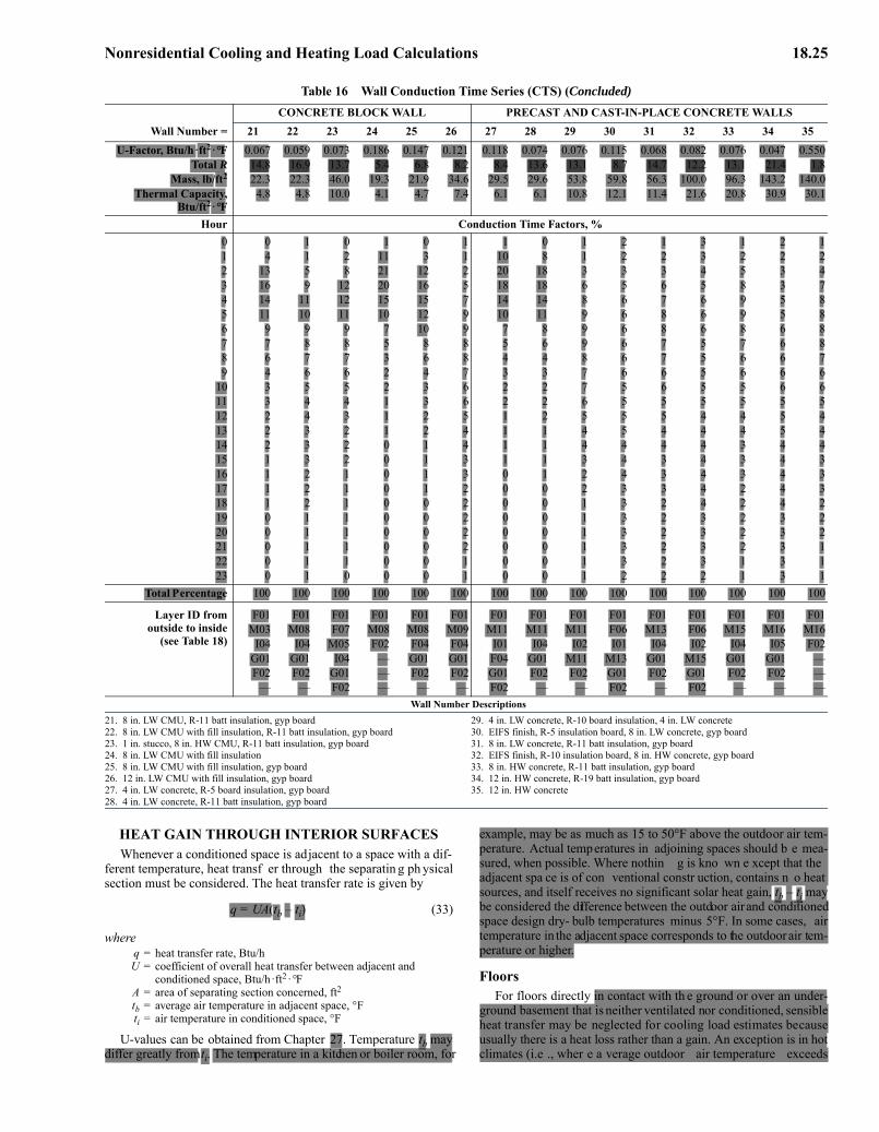
Nonresidential Cooling and Heating Load Calculations 18.25

HEAT GAIN THROUGH INTERIOR SURFACESWhenever a conditioned space is adjacent to a space with a dif-

ferent temperature, heat transf er through the separatin g ph ysicalsection must be considered. The heat transfer rate is given by

q = UA(tb – ti) (33)

whereq = heat transfer rate, Btu/hU = coefficient of overall heat transfer between adjacent and

conditioned space, Btu/h·ft2·°FA = area of separating section concerned, ft2tb = average air temperature in adjacent space, °Fti = air temperature in conditioned space, °F

U-values can be obtained from Chapter 27. Temperature tb maydiffer greatly from ti. The temperature in a kitchen or boiler room, for

example, may be as much as 15 to 50°F above the outdoor air tem-perature. Actual temperatures in adjoining spaces should b e mea-sured, when possible. Where nothin g is kno wn e xcept that theadjacent spa ce is of con ventional constr uction, contains n o heatsources, and itself receives no significant solar heat gain, tb – ti maybe considered the difference between the outdoor air and conditionedspace design dry- bulb temperatures minus 5°F. In some cases, airtemperature in the adjacent space corresponds to the outdoor air tem-perature or higher.

FloorsFor floors directly in contact with th e ground or over an under-

ground basement that is neither ventilated nor conditioned, sensibleheat transfer may be neglected for cooling load estimates becauseusually there is a heat loss rather than a gain. An exception is in hotclimates (i.e ., wher e a verage outdoor air temperature exceeds

Table 16 Wall Conduction Time Series (CTS) (Concluded)

Wall Number =CONCRETE BLOCK WALL PRECAST AND CAST-IN-PLACE CONCRETE WALLS

21 22 23 24 25 26 27 28 29 30 31 32 33 34 35U-Factor, Btu/h·ft2·°F 0.067 0.059 0.073 0.186 0.147 0.121 0.118 0.074 0.076 0.115 0.068 0.082 0.076 0.047 0.550

Total R 14.8 16.9 13.7 5.4 6.8 8.2 8.4 13.6 13.1 8.7 14.7 12.2 13.1 21.4 1.8Mass, lb/ft2 22.3 22.3 46.0 19.3 21.9 34.6 29.5 29.6 53.8 59.8 56.3 100.0 96.3 143.2 140.0

Thermal Capacity,Btu/ft2·°F

4.8 4.8 10.0 4.1 4.7 7.4 6.1 6.1 10.8 12.1 11.4 21.6 20.8 30.9 30.1

Hour Conduction Time Factors, %0 0 1 0 1 0 1 1 0 1 2 1 3 1 2 11 4 1 2 11 3 1 10 8 1 2 2 3 2 2 22 13 5 8 21 12 2 20 18 3 3 3 4 5 3 43 16 9 12 20 16 5 18 18 6 5 6 5 8 3 74 14 11 12 15 15 7 14 14 8 6 7 6 9 5 85 11 10 11 10 12 9 10 11 9 6 8 6 9 5 86 9 9 9 7 10 9 7 8 9 6 8 6 8 6 87 7 8 8 5 8 8 5 6 9 6 7 5 7 6 88 6 7 7 3 6 8 4 4 8 6 7 5 6 6 79 4 6 6 2 4 7 3 3 7 6 6 5 6 6 6

10 3 5 5 2 3 6 2 2 7 5 6 5 5 6 611 3 4 4 1 3 6 2 2 6 5 5 5 5 5 512 2 4 3 1 2 5 1 2 5 5 5 4 4 5 413 2 3 2 1 2 4 1 1 4 5 4 4 4 5 414 2 3 2 0 1 4 1 1 4 4 4 4 3 4 415 1 3 2 0 1 3 1 1 3 4 3 4 3 4 316 1 2 1 0 1 3 0 1 2 4 3 4 3 4 317 1 2 1 0 1 2 0 0 2 3 3 4 2 4 318 1 2 1 0 0 2 0 0 1 3 2 4 2 4 219 0 1 1 0 0 2 0 0 1 3 2 3 2 3 220 0 1 1 0 0 2 0 0 1 3 2 3 2 3 221 0 1 1 0 0 2 0 0 1 3 2 3 2 3 122 0 1 1 0 0 1 0 0 1 3 2 3 1 3 123 0 1 0 0 0 1 0 0 1 2 2 2 1 3 1

Total Percentage 100 100 100 100 100 100 100 100 100 100 100 100 100 100 100

Layer ID fromoutside to inside

(see Table 18)

F01 F01 F01 F01 F01 F01 F01 F01 F01 F01 F01 F01 F01 F01 F01M03 M08 F07 M08 M08 M09 M11 M11 M11 F06 M13 F06 M15 M16 M16

I04 I04 M05 F02 F04 F04 I01 I04 I02 I01 I04 I02 I04 I05 F02G01 G01 I04 — G01 G01 F04 G01 M11 M13 G01 M15 G01 G01 —F02 F02 G01 — F02 F02 G01 F02 F02 G01 F02 G01 F02 F02 —

— — F02 — — — F02 — — F02 — F02 — — —Wall Number Descriptions

21. 8 in. LW CMU, R-11 batt insulation, gyp board22. 8 in. LW CMU with fill insulation, R-11 batt insulation, gyp board23. 1 in. stucco, 8 in. HW CMU, R-11 batt insulation, gyp board24. 8 in. LW CMU with fill insulation25. 8 in. LW CMU with fill insulation, gyp board26. 12 in. LW CMU with fill insulation, gyp board27. 4 in. LW concrete, R-5 board insulation, gyp board28. 4 in. LW concrete, R-11 batt insulation, gyp board

29. 4 in. LW concrete, R-10 board insulation, 4 in. LW concrete30. EIFS finish, R-5 insulation board, 8 in. LW concrete, gyp board31. 8 in. LW concrete, R-11 batt insulation, gyp board32. EIFS finish, R-10 insulation board, 8 in. HW concrete, gyp board33. 8 in. HW concrete, R-11 batt insulation, gyp board34. 12 in. HW concrete, R-19 batt insulation, gyp board35. 12 in. HW concrete

18.26 2009 ASHRAE Handbook—Fundamentals

indoor design condition), where the positive soil-to-indoor temper-ature difference causes sensible heat g ains (Rock 2 005). In manyclimates and fo r various te mperatures and local soil cond itions,moisture transport up through slabs-on-grade and basement floors isalso signif icant, an d contributes to the latent heat portion of th ecooling load.

CALCULATING COOLING LOADThe instantaneous cooling load is the rate at which heat energy

is convected to the zone air at a given point in time. Computation ofcooling load is complicated by the ra diant e xchange be tween

surfaces, furniture, partitions, and other mass in the zone. Most heatgain sources transfer energy by both convection and radiation. Radi-ative heat transfer introduces a time dependency to the process thatis not easily quantified. Radiation is absorbed by thermal masses inthe zone and then later transferred by convection into the space. Thisprocess c reates a time lag and dampen ing effect. The convectiveportion, on the other hand, is assumed to immediately become cool-ing load in the hour in which that heat gain occurs.

Heat balance procedures calculate the radiant exchange betweensurfaces ba sed on thei r surface te mperatures and em issivities, butthey typically rely on estimated “radiative/convective splits” to deter-mine the contribution of i nternal loads, including people, ligh ting,

Table 17 Roof Conduction Time Series (CTS)

SLOPED FRAME ROOFS WOOD DECK METAL DECK ROOFS CONCRETE ROOFSRoof Number 1 2 3 4 5 6 7 8 9 10 11 12 13 14 15 16 17 18 19

U-Factor,Btu/h·ft2·°F

0.044 0.040 0.045 0.041 0.042 0.041 0.069 0.058 0.080 0.065 0.057 0.036 0.052 0.054 0.052 0.051 0.056 0.055 0.042

Total R 22.8 25.0 22.2 24.1 23.7 24.6 14.5 17.2 12.6 15.4 17.6 27.6 19.1 18.6 19.2 19.7 18.0 18.2 23.7Mass, lb/ft2 5.5 4.3 2.9 7.1 11.4 7.1 10.0 11.5 4.9 6.3 5.1 5.6 11.8 30.6 43.9 57.2 73.9 97.2 74.2

Thermal Capacity,Btu/ft2·°F

1.3 0.8 0.6 2.3 3.6 2.3 3.7 3.9 1.4 1.6 1.4 1.6 2.8 6.6 9.3 12.0 16.3 21.4 16.2

Hour Conduction Time Factors, %0 6 10 27 1 1 1 0 1 18 4 8 1 0 1 2 2 2 3 11 45 57 62 17 17 12 7 3 61 41 53 23 10 2 2 2 2 3 22 33 27 10 31 34 25 18 8 18 35 30 38 22 8 3 3 5 3 63 11 5 1 24 25 22 18 10 3 14 7 22 20 11 6 4 6 5 84 3 1 0 14 13 15 15 10 0 4 2 10 14 11 7 5 7 6 85 1 0 0 7 6 10 11 9 0 1 0 4 10 10 8 6 7 6 86 1 0 0 4 3 6 8 8 0 1 0 2 7 9 8 6 6 6 77 0 0 0 2 1 4 6 7 0 0 0 0 5 7 7 6 6 6 78 0 0 0 0 0 2 5 6 0 0 0 0 4 6 7 6 6 6 69 0 0 0 0 0 1 3 5 0 0 0 0 3 5 6 6 5 5 5

10 0 0 0 0 0 1 3 5 0 0 0 0 2 5 5 6 5 5 511 0 0 0 0 0 1 2 4 0 0 0 0 1 4 5 5 5 5 512 0 0 0 0 0 0 1 4 0 0 0 0 1 3 5 5 4 5 413 0 0 0 0 0 0 1 3 0 0 0 0 1 3 4 5 4 4 414 0 0 0 0 0 0 1 3 0 0 0 0 0 3 4 4 4 4 315 0 0 0 0 0 0 1 3 0 0 0 0 0 2 3 4 4 4 316 0 0 0 0 0 0 0 2 0 0 0 0 0 2 3 4 3 4 317 0 0 0 0 0 0 0 2 0 0 0 0 0 2 3 4 3 4 318 0 0 0 0 0 0 0 2 0 0 0 0 0 1 3 3 3 3 219 0 0 0 0 0 0 0 2 0 0 0 0 0 1 2 3 3 3 220 0 0 0 0 0 0 0 1 0 0 0 0 0 1 2 3 3 3 221 0 0 0 0 0 0 0 1 0 0 0 0 0 1 2 3 3 3 222 0 0 0 0 0 0 0 1 0 0 0 0 0 1 2 3 2 2 223 0 0 0 0 0 0 0 0 0 0 0 0 0 1 1 2 2 2 2

100 100 100 100 100 100 100 100 100 100 100 100 100 100 100 100 100 100 100

Layer IDfrom outside to

inside(see Table 18)

F01 F01 F01 F01 F01 F01 F01 F01 F01 F01 F01 F01 F01 F01 F01 F01 F01 F01 F01F08 F08 F08 F12 F14 F15 F13 F13 F13 F13 F13 F13 M17 F13 F13 F13 F13 F13 F13G03 G03 G03 G05 G05 G05 G03 G03 G03 G03 G03 G03 F13 G03 G03 G03 G03 G03 M14F05 F05 F05 F05 F05 F05 I02 I02 I02 I02 I03 I02 G03 I03 I03 I03 I03 I03 F05I05 I05 I05 I05 I05 I05 G06 G06 F08 F08 F08 I03 I03 M11 M12 M13 M14 M15 I05

G01 F05 F03 F05 F05 F05 F03 F05 F03 F05 F03 F08 F08 F03 F03 F03 F03 F03 F16F03 F16 — G01 G01 G01 — F16 — F16 — — F03 — — — — — F03

— F03 — F03 F03 F03 — F03 — F03 — — — — — — — — —Roof Number Descriptions

1. Metal roof, R-19 batt insulation, gyp board2. Metal roof, R-19 batt insulation, suspended acoustical ceiling3. Metal roof, R-19 batt insulation4. Asphalt shingles, wood sheathing, R-19 batt insulation, gyp board5. Slate or tile, wood sheathing, R-19 batt insulation, gyp board6. Wood shingles, wood sheathing, R-19 batt insulation, gyp board7. Membrane, sheathing, R-10 insulation board, wood deck8. Membrane, sheathing, R-10 insulation board, wood deck, suspended acoustical ceiling9. Membrane, sheathing, R-10 insulation board, metal deck10. Membrane, sheathing, R-10 insulation board, metal deck, suspended acoustical ceiling

11. Membrane, sheathing, R-15 insulation board, metal deck12. Membrane, sheathing, R-10 plus R-15 insulation boards, metal deck13. 2 in. concrete roof ballast, membrane, sheathing, R-15 insulation board, metal deck14. Membrane, sheathing, R-15 insulation board, 4 in. LW concrete15. Membrane, sheathing, R-15 insulation board, 6 in. LW concrete16. Membrane, sheathing, R-15 insulation board, 8 in. LW concrete17. Membrane, sheathing, R-15 insulation board, 6 in. HW concrete18. Membrane, sheathing, R-15 insulation board, 8 in. HW concrete19. Membrane, 6-in HW concrete, R-19 batt insulation, suspended acoustical ceiling

Nonresidential Cooling and Heating Load Calculations 18.27

Table 18 Thermal Properties and Code Numbers of Layers Used in Wall and Roof Descriptions for Tables 16 and 17

Layer ID Description

Thickness, in.

Conductivity, Btu·in/h·ft2·°F

Density, lb/ft3

Specific Heat,

Btu/lb·°FResistance,

ft2·°F·h/Btu RMass, lb/ft2

Thermal Capacity, Btu/ft2·°F Notes

F01 Outside surface resistance — — — — 0.25 0.25 — — 1F02 Inside vertical surface resistance — — — — 0.68 0.68 — — 2F03 Inside horizontal surface resistance — — — — 0.92 0.92 — — 3F04 Wall air space resistance — — — — 0.87 0.87 — — 4F05 Ceiling air space resistance — — — — 1.00 1.00 — — 5F06 EIFS finish 0.375 5.00 116.0 0.20 — 0.08 3.63 0.73 6F07 1 in. stucco 1.000 5.00 116.0 0.20 — 0.20 9.67 1.93 6F08 Metal surface 0.030 314.00 489.0 0.12 — 0.00 1.22 0.15 7F09 Opaque spandrel glass 0.250 6.90 158.0 0.21 — 0.04 3.29 0.69 8F10 1 in. stone 1.000 22.00 160.0 0.19 — 0.05 13.33 2.53 9F11 Wood siding 0.500 0.62 37.0 0.28 — 0.81 1.54 0.43 10F12 Asphalt shingles 0.125 0.28 70.0 0.30 — 0.44 0.73 0.22F13 Built-up roofing 0.375 1.13 70.0 0.35 — 0.33 2.19 0.77F14 Slate or tile 0.500 11.00 120.0 0.30 — 0.05 5.00 1.50F15 Wood shingles 0.250 0.27 37.0 0.31 — 0.94 0.77 0.24F16 Acoustic tile 0.750 0.42 23.0 0.14 — 1.79 1.44 0.20 11F17 Carpet 0.500 0.41 18.0 0.33 — 1.23 0.75 0.25 12F18 Terrazzo 1.000 12.50 160.0 0.19 — 0.08 13.33 2.53 13G01 5/8 in. gyp board 0.625 1.11 50.0 0.26 — 0.56 2.60 0.68G02 5/8 in. plywood 0.625 0.80 34.0 0.29 — 0.78 1.77 0.51G03 1/2 in. fiberboard sheathing 0.500 0.47 25.0 0.31 — 1.06 1.04 0.32 14G04 1/2 in. wood 0.500 1.06 38.0 0.39 — 0.47 1.58 0.62 15G05 1 in. wood 1.000 1.06 38.0 0.39 — 0.94 3.17 1.24 15G06 2 in. wood 2.000 1.06 38.0 0.39 — 1.89 6.33 2.47 15G07 4 in. wood 4.000 1.06 38.0 0.39 — 3.77 12.67 4.94 15I01 R-5, 1 in. insulation board 1.000 0.20 2.7 0.29 — 5.00 0.23 0.07 16I02 R-10, 2 in. insulation board 2.000 0.20 2.7 0.29 — 10.00 0.45 0.13 16I03 R-15, 3 in. insulation board 3.000 0.20 2.7 0.29 — 15.00 0.68 0.20 16I04 R-11, 3-1/2 in. batt insulation 3.520 0.32 1.2 0.23 — 11.00 0.35 0.08 17I05 R-19, 6-1/4 in. batt insulation 6.080 0.32 1.2 0.23 — 19.00 0.61 0.14 17I06 R-30, 9-1/2 in. batt insulation 9.600 0.32 1.2 0.23 — 30.00 0.96 0.22 17

M01 4 in. brick 4.000 6.20 120.0 0.19 — 0.65 40.00 7.60 18M02 6 in. LW concrete block 6.000 3.39 32.0 0.21 — 1.77 16.00 3.36 19M03 8 in. LW concrete block 8.000 3.44 29.0 0.21 — 2.33 19.33 4.06 20M04 12 in. LW concrete block 12.000 4.92 32.0 0.21 — 2.44 32.00 6.72 21M05 8 in. concrete block 8.000 7.72 50.0 0.22 — 1.04 33.33 7.33 22M06 12 in. concrete block 12.000 9.72 50.0 0.22 — 1.23 50.00 11.00 23M07 6 in. LW concrete block (filled) 6.000 1.98 32.0 0.21 — 3.03 16.00 3.36 24M08 8 in. LW concrete block (filled) 8.000 1.80 29.0 0.21 — 4.44 19.33 4.06 25M09 12 in. LW concrete block (filled) 12.000 2.04 32.0 0.21 — 5.88 32.00 6.72 26M10 8 in. concrete block (filled) 8.000 5.00 50.0 0.22 — 1.60 33.33 7.33 27M11 4 in. lightweight concrete 4.000 3.70 80.0 0.20 — 1.08 26.67 5.33M12 6 in. lightweight concrete 6.000 3.70 80.0 0.20 — 1.62 40.00 8.00M13 8 in. lightweight concrete 8.000 3.70 80.0 0.20 — 2.16 53.33 10.67M14 6 in. heavyweight concrete 6.000 13.50 140.0 0.22 — 0.44 70.00 15.05M15 8 in. heavyweight concrete 8.000 13.50 140.0 0.22 — 0.48 93.33 20.07M16 12 in. heavyweight concrete 12.000 13.50 140.0 0.22 — 0.89 140.0 30.10M17 2 in. LW concrete roof ballast 2.000 1.30 40 0.20 — 1.54 6.7 1.33 28

Notes: The following notes give sources for the data in this table.1. Chapter 26, Table 1 for 7.5 mph wind2. Chapter 26, Table 1 for still air, horizontal heat flow3. Chapter 26, Table 1 for still air, downward heat flow4. Chapter 26, Table 3 for 1.5 in. space, 90°F, horizontal heat flow, 0.82 emittance5. Chapter 26, Table 3 for 3.5 in. space, 90°F, downward heat flow, 0.82 emittance6. EIFS finish layers approximated by Chapter 26, Table 4 for 3/8 in. cement plaster,

sand aggregate7. Chapter 33, Table 3 for steel (mild)8. Chapter 26, Table 4 for architectural glass9. Chapter 26, Table 4 for marble and granite

10. Chapter 26, Table 4, density assumed same as Southern pine11. Chapter 26, Table 4 for mineral fiberboard, wet molded, acoustical tile12. Chapter 26, Table 4 for carpet and rubber pad, density assumed same as fiberboard13. Chapter 26, Table 4, density assumed same as stone

14. Chapter 26, Table 4 for nail-base sheathing15. Chapter 26, Table 4 for Southern pine16. Chapter 26, Table 4 for expanded polystyrene17. Chapter 26, Table 4 for glass fiber batt, specific heat per glass fiber board18. Chapter 26, Table 4 for clay fired brick19. Chapter 26, Table 4, 16 lb block, 8 × 16 in. face20. Chapter 26, Table 4, 19 lb block, 8 × 16 in. face21. Chapter 26, Table 4, 32 lb block, 8 × 16 in. face22. Chapter 26, Table 4, 33 lb normal weight block, 8 × 16 in. face23. Chapter 26, Table 4, 50 lb normal weight block, 8 × 16 in. face24. Chapter 26, Table 4, 16 lb block, vermiculite fill25. Chapter 26, Table 4, 19 lb block, 8 × 16 in. face, vermiculite fill26. Chapter 26, Table 4, 32 lb block, 8 × 16 in. face, vermiculite fill27. Chapter 26, Table 4, 33 lb normal weight block, 8 × 16 in. face, vermiculite fill28. Chapter 26, Table 4 for 40 lb/ft3 LW concrete

18.28 2009 ASHRAE Handbook—Fundamentals

appliances, and equipment, to the radiant exchange. RTS further sim-plifies th e HB procedure by also rely ing on an estimated radia-tive/convective split of wall and roof conductive heat gain instead ofsimultaneously solving for the instantaneous convective and radiativeheat transfer from each surface, as is done in the HB procedure.

Thus, the cooling load for each load component (lights, people,walls, roofs, windows, appliances, etc.) for a particular hour is thesum of the convective portion of the heat gain for that hour plus thetime-delayed portion of radiant heat gains for that hour and the pre-vious 23 h. Table 14 contains recommendations for splitting each ofthe heat gain components into convective and radiant portions.

RTS converts the radiant portion of hourly heat g ains to hourlycooling loads using radiant time factors, the coefficients of the radi-ant time series. Radiant time factors are used to calculate the coolingload for the current hour on the basis of current and past heat gains.The radiant time series for a particular zone gives the time-dependentresponse of the zone to a single pulse of radiant energy. The seriesshows the portion of the radiant pulse that is convected to zone air foreach hour. Thus, r0 represents the fraction of the radiant pulse con-vected to the zone air in the current hour r1 in the previous hour, andso on. The radiant time series thus generated is used to convert theradiant portion of hourly heat gains to hourly cooling loads accord-ing to the following equation:

Qr,θ = r0qr,θ + r1qr,θ –1 + r2qr,θ –2 + r3qr,θ –3 + … + r23qr,θ –23 (34)

whereQr, θ =radiant cooling load Qr for current hour θ, Btu/hqr, θ =radiant heat gain for current hour, Btu/h

qr,θ−n =radiant heat gain n hours ago, Btu/hr0, r1, etc.=radiant time factors

The radiant cooling load for the current hour, which is calculatedusing RTS and Equation (34), is added to the convective portion todetermine the total cooling load for that component for that hour.

Radiant time factors are generated by a heat balance based proce-dure. A separate series of radiant time factors is theoretically requiredfor each unique zone and for each unique radiant energy distributionfunction assumption. F or most co mmon design appli cations, RTSvariation depends primarily on the o verall massiveness of t heconstruction and the thermal responsiveness of the surfaces the radi-ant heat gains strike.

One goal in developing RTS was to provide a simplified methodbased directly on the HB method; thus, it was deemed desirable togenerate RTS coefficients directly from a heat balance. A heat bal-ance computer program was developed to do this: Hbfort, which isincluded as part of Cooling and Heating Load Calculation Princi-ples (Pedersen et al. 1998) . The R TS procedure is described bySpitler et al. (1997). The procedure for generating RTS coefficientsmay be thought of as analogous to the custom weighting f actorgeneration procedure used by DOE 2.1 (Kerrisk et al. 1981; Sowell1988a, 1988b). In both cases, a z one model is pulsed with a heatgain. With DOE 2.1, the resulting loads are used to estimate the bestvalues of the transfer fu nction method weighting f actors to mostclosely match the load prof ile. In the procedure described here, aunit periodic heat g ain pulse is used to generate loads for a 24 hperiod. As long as the heat gain pulse is a unit pulse, the resultingloads are equivalent to the RTS coefficients.

Two different radiant time series are used: Solar, for direct trans-mitted solar heat gain (radiant energy assumed to be distributed tothe floor and furnishings only) and nonsolar, for all other types ofheat gains (radiant energy assumed to be uniformly distributed onall internal surfaces). Nonsolar RTS apply to radiant heat gains frompeople, lights, appliances, walls, roofs, and floors. Also, for diffusesolar hea t g ain and di rect solar heat ga in fro m fen estration withinside shading (blinds, drapes, etc.), the nonsolar RTS should b eused. Radiation from those sources is assumed to be more uniformly

distributed onto all room surfaces. Effect of bea m solar radiationdistribution assumptions is addressed by Hittle (1999).

Representative solar and nonsolar RTS data for light, medium,and heavyweight constructions are pro vided in Tables 19 and 20.Those were calculated using the Hbfort computer program (Peder-sen et al. 1998) with zone characteristics listed in Table 21. Custom-ized RTS values may be calculated using the HB method where thezone is not reasonably similar to these typical zones or where moreprecision is desired.

ASHRAE research project RP-942 compared HB and R TS re-sults over a wide range of zone types and input variables (Rees et al.2000; Spitler et al. 1998). In general, total cooling loads calculatedusing RTS closely agreed with or were slightly higher than those ofthe HB method with the same inputs. The project examined morethan 5000 test cases of varying zone parameters. Th e dominatingvariable was overall thermal mass, and results were grouped intolightweight, U.S. me dium-weight, U.K. medium-weight, andheavyweight construction. Best agreement between RTS and HB re-sults was obtained fo r light- an d medium-weight construction.Greater differences occurred in heavyweight cases, with RTS gen-erally predicting slightly highe r peak cooling loads than HB.Greater dif ferences al so were obser ved in zone s wit h e xtremelyhigh internal radiant loads an d large glazing areas or w ith a v erylightweight exterior envelope. In this case, heat balance calculationspredict that some of the internal radiant load will be transmitted tothe outdoor environment and never becomes cooling load within thespace. RTS does not account for energy transfer out of the space tothe environment, and thus predicted higher cooling loads.

ASHRAE research project RP-1 117 co nstructed tw o modelrooms for which cooling loads were physically measured usingextensive instrumentation. The results agreed with previous simula-tions (Chantrasrisalai et al. 2003; Eldridge et al. 2003; Iu et al. 2003).HB calculations closely approximated the measured cooling loa dswhen provided with detailed data for the test room s. RTS overpre-dicted measured cooling loads in tests with large, clear, single-glazedwindow areas with bare concrete floor and no furnishings or internalloads. Tests under more typical conditions (venetian blinds, carpetedfloor, office-type furnishings, and normal internal loads) providedgood agreement between HB, RTS, and measured loads.

HEATING LOAD CALCULATIONSTechniques for estimating design heating load for commercial,

institutional, and industrial applications are essentially the same asfor those estimating design cooling loads for such uses, with the fol-lowing exceptions:

• Temperatures outside conditioned spaces are generally lower thanmaintained space temperatures.

• Credit for solar or internal heat gains is not included• Thermal storage effect of building structure or content is ignored.• Thermal bridging effects on wall and roof conduction are greater

for heating loads than for cooling loads, and greater care must betaken to account for bridging effects on U-factors used in heatingload calculations.

Heat losses (negative heat gains) are thus considered to be instan-taneous, heat transfer essentially conductive, and latent heat treatedonly as a functio n of replacing sp ace humidity lost to the exteriorenvironment.

This simplified approach is justified because it evaluates worst-case conditions that can reasonably occur during a heating season.Therefore, the near-worst-case load is based on the following:

• Design interior and exterior conditions• Including infiltration and/or ventilation• No solar effect (at night or on cloudy winter days)• Before the periodic presence of people, lights, and appliances has

an offsetting effect

Nonresidential Cooling and Heating Load Calculations 18.29

Table 19 Representative Nonsolar RTS Values for Light to Heavy Construction

%Glass

Interior Zones Light Medium Heavy Light Medium Heavy

With Carpet No Carpet With Carpet No Carpet With Carpet No Carpet

With

Car

pet

No

Car

pet

With

Car

pet

No

Car

pet

With

Car

pet

No

Car

pet

10% 50% 90% 10% 50% 90% 10% 50% 90% 10% 50% 90% 10% 50% 90% 10% 50% 90%Hour Radiant Time Factor, %

0 47 50 53 41 43 46 46 49 52 31 33 35 34 38 42 22 25 28 46 40 46 31 33 211 19 18 17 20 19 19 18 17 16 17 16 15 9 9 9 10 9 9 19 20 18 17 9 92 11 10 9 12 11 11 10 9 8 11 10 10 6 6 5 6 6 6 11 12 10 11 6 63 6 6 5 8 7 7 6 5 5 8 7 7 4 4 4 5 5 5 6 8 6 8 5 54 4 4 3 5 5 5 4 3 3 6 5 5 4 4 4 5 5 4 4 5 3 6 4 55 3 3 2 4 3 3 2 2 2 4 4 4 4 3 3 4 4 4 3 4 2 4 4 46 2 2 2 3 3 2 2 2 2 4 3 3 3 3 3 4 4 4 2 3 2 4 3 47 2 1 1 2 2 2 1 1 1 3 3 3 3 3 3 4 4 4 2 2 1 3 3 48 1 1 1 1 1 1 1 1 1 3 2 2 3 3 3 4 3 3 1 1 1 3 3 49 1 1 1 1 1 1 1 1 1 2 2 2 3 3 2 3 3 3 1 1 1 2 3 3

10 1 1 1 1 1 1 1 1 1 2 2 2 3 2 2 3 3 3 1 1 1 2 3 311 1 1 1 1 1 1 1 1 1 2 2 2 2 2 2 3 3 3 1 1 1 2 2 312 1 1 1 1 1 1 1 1 1 1 1 1 2 2 2 3 3 3 1 1 1 1 2 313 1 1 1 0 1 0 1 1 1 1 1 1 2 2 2 3 3 2 1 1 1 1 2 314 0 0 1 0 1 0 1 1 1 1 1 1 2 2 2 3 2 2 1 0 1 1 2 315 0 0 1 0 0 0 1 1 1 1 1 1 2 2 2 2 2 2 0 0 1 1 2 316 0 0 0 0 0 0 1 1 1 1 1 1 2 2 2 2 2 2 0 0 1 1 2 317 0 0 0 0 0 0 1 1 1 1 1 1 2 2 2 2 2 2 0 0 1 1 2 218 0 0 0 0 0 0 1 1 1 1 1 1 2 2 1 2 2 2 0 0 1 1 2 219 0 0 0 0 0 0 0 1 0 0 1 1 2 2 1 2 2 2 0 0 1 0 2 220 0 0 0 0 0 0 0 0 0 0 1 1 2 1 1 2 2 2 0 0 0 0 2 221 0 0 0 0 0 0 0 0 0 0 1 1 2 1 1 2 2 2 0 0 0 0 2 222 0 0 0 0 0 0 0 0 0 0 1 0 1 1 1 2 2 2 0 0 0 0 1 223 0 0 0 0 0 0 0 0 0 0 0 0 1 1 1 2 2 1 0 0 0 0 1 2

100 100 100 100 100 100 100 100 100 100 100 100 100 100 100 100 100 100 100 100 100 100 100 100

Table 20 Representative Solar RTS Values for Light to Heavy Construction

%Glass

Light Medium HeavyWith Carpet No Carpet With Carpet No Carpet With Carpet No Carpet

10% 50% 90% 10% 50% 90% 10% 50% 90% 10% 50% 90% 10% 50% 90% 10% 50% 90%Hour Radiant Time Factor, %

0 53 55 56 44 45 46 52 54 55 28 29 29 47 49 51 26 27 281 17 17 17 19 20 20 16 16 15 15 15 15 11 12 12 12 13 132 9 9 9 11 11 11 8 8 8 10 10 10 6 6 6 7 7 73 5 5 5 7 7 7 5 4 4 7 7 7 4 4 3 5 5 54 3 3 3 5 5 5 3 3 3 6 6 6 3 3 3 4 4 45 2 2 2 3 3 3 2 2 2 5 5 5 2 2 2 4 4 46 2 2 2 3 2 2 2 1 1 4 4 4 2 2 2 3 3 37 1 1 1 2 2 2 1 1 1 4 3 3 2 2 2 3 3 38 1 1 1 1 1 1 1 1 1 3 3 3 2 2 2 3 3 39 1 1 1 1 1 1 1 1 1 3 3 3 2 2 2 3 3 3

10 1 1 1 1 1 1 1 1 1 2 2 2 2 2 2 3 3 311 1 1 1 1 1 1 1 1 1 2 2 2 2 2 1 3 3 212 1 1 1 1 1 0 1 1 1 2 2 2 2 1 1 2 2 213 1 1 0 1 0 0 1 1 1 2 2 2 2 1 1 2 2 214 1 0 0 0 0 0 1 1 1 1 1 1 2 1 1 2 2 215 1 0 0 0 0 0 1 1 1 1 1 1 1 1 1 2 2 216 0 0 0 0 0 0 1 1 1 1 1 1 1 1 1 2 2 217 0 0 0 0 0 0 1 1 1 1 1 1 1 1 1 2 2 218 0 0 0 0 0 0 1 1 1 1 1 1 1 1 1 2 2 219 0 0 0 0 0 0 0 0 0 1 1 1 1 1 1 2 2 220 0 0 0 0 0 0 0 0 0 1 1 1 1 1 1 2 2 221 0 0 0 0 0 0 0 0 0 0 0 0 1 1 1 2 2 222 0 0 0 0 0 0 0 0 0 0 0 0 1 1 1 2 1 123 0 0 0 0 0 0 0 0 0 0 0 0 1 1 1 2 1 1

100 100 100 100 100 100 100 100 100 100 100 100 100 100 100 100 100 100

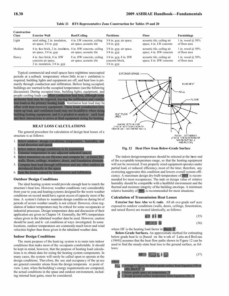
18.30 2009 ASHRAE Handbook—Fundamentals

Typical commercial and retail spaces have nighttime unoccupiedperiods at a setback temperature where little to no v entilation i srequired, building lights and equipment are off, and heat loss is pri-marily through conduction and infiltration. Before being occupied,buildings are warmed to the occupied temperature (see the followingdiscussion). During occupied time, building lights, equipment, andpeople cooling loads can offset conduction heat loss, although someperimeter heat may be required, leaving the infiltration and ventila-tion loads as the primary heating loads. Ventilation heat load may beoffset with heat recovery equipment. These loads (conduction loss,warm-up load, and ventilation load) may not be additive when sizingbuilding heating equipment, and it is prudent to analyze each loadand their interactions to arrive at final equipment sizing for heating.

HEAT LOSS CALCULATIONSThe general procedure for calculation of design heat losses of a

structure is as follows:1. Select outdoor design con ditions: temperature, humidity, and

wind direction and speed.2. Select indoor design conditions to be maintained.3. Estimate temperature in any adjacent unheated spaces.4. Select transmissi on coe fficients and compute he at losses for

walls, floors, ceilings, windows, doors, and foundation elements.5. Compute heat load through infiltration and any other outdoor air

introduced directly to the space.6. Sum the losses caused by transmission and infiltration.

Outdoor Design ConditionsThe ideal heating system would provide enough heat to match the

structure’s heat loss. However, weather conditions vary considerablyfrom year to year, and heating systems designed for the worst weatherconditions on record would have a great excess of capacity most of thetime. A system’s failure to maintain design conditio ns during bri efperiods of severe weather usually is not critical. However, close reg-ulation of indoor temperature may be critical for some occupancies orindustrial processes. Design temperature data and discussion of theirapplication are given in Chapter 14. Generally, the 99% temperaturevalues given in the tabulated weather data be used. However, cautionshould be used, and lo cal conditions al ways investigated. In somelocations, outdoor temperatures are commonly much lower and windvelocities higher than those given in the tabulated weather data.

Indoor Design ConditionsThe main purpose of the heati ng system is to main tain indoor

conditions that make most of the occupants comfortable. It shouldbe kept in mind, however, that the purpose of heating load calcula-tions is to obtain data for sizing the heating system components. Inmany cases, the system will rarely be called upon to operate at thedesign conditions. Ther efore, the use and occupancy of the sp aceare general consider ations from the design temperatu re point ofview. Later, when the building’s energy requirements are computed,the actual conditions in the space and outdoor environment, includ-ing internal heat gains, must be considered.

The indoor design temperature should be selected at the lower endof the acceptable temperature range, so that the heating equipmentwill not be oversized. Even properly sized equipment operates underpartial load, a t reduced efficiency, most of t he time; therefore, anyoversizing aggravates this condition and lowers overall system effi-ciency. A maximum design dry-bulb temperature of 70°F is recom-mended for most occupancies. The indo or design value of relativehumidity should be compatible with a healthful environment and thethermal and moisture integrity of the building envelope. A minimumrelative humidity of 30% is recommended for most situations.

Calculation of Transmission Heat LossesExterior Sur face Abo ve G rade. All ab ove-grade surf aces

exposed to outdoor conditions (walls, doors, ceilings, fenestration,and raised floors) are treated identically, as follows:

(35)

(36)

where HF is the heating load factor in Btu/h·ft2.Below-Grade Surfaces. An approximate method for estimating

below-grade heat lo ss [based on the w ork of Latta an d Boil eau(1969)] assumes that the heat flow paths shown in Figure 12 can beused to find the steady-state heat loss to the ground surface, as fol-lows:

(37)

whereUavg = average U-factor for below-grade surface from Equation (39) or

(40), Btu/h·ft2·°Ftin = below-grade space air temperature, °Ftgr = design ground surface temperature from Equation (38), °F

Table 21 RTS Representative Zone Construction for Tables 19 and 20

ConstructionClass Exterior Wall Roof/Ceiling Partitions Floor FurnishingsLight steel siding, 2 in. insulation,

air space, 3/4 in. gyp4 in. LW concrete, ceiling air space, acoustic tile

3/4 in. gyp, air space, 3/4 in. gyp

acoustic tile, ceiling air space, 4 in. LW concrete

1 in. wood @ 50% of floor area

Medium 4 in. face brick, 2 in. insulation, air space, 3/4 in. gyp

4 in. HW concrete, ceiling air space, acoustic tile

3/4 in. gyp, air space, 3/4 in. gyp

acoustic tile, ceiling air space, 4 in. HW concrete

1 in. wood @ 50% of floor area

Heavy 4 in. face brick, 8 in. HW concrete air space, 2 in. insulation, 3/4 in. gyp

8 in. HW concrete, ceiling air space, acoustic tile

3/4 in. gyp, 8 in. HW concrete block, 3/4 in. gyp

acoustic tile, ceiling air space, 8 in. HW concrete

1 in. wood @ 50% of floor area

q A HF×=

HF U tΔ=

Fig. 12 Heat Flow from Below-Grade Surface

Fig. 12 Heat Flow from Below-Grade Surface

HF Uavg tin tgr–( )=

Nonresidential Cooling and Heating Load Calculations 18.31

The ef fect of soil heat capacity means that none of the usualexternal design air temperatures are suitable values for tgr. Groundsurface temperature fluctuates about an annual mean v alue byamplitude A, which v aries with geographic location and surf acecover. The minimum ground surface temperature, suitable for heatloss estimates, is therefore

(38)

where= mean ground temperature, °F, estimated from the annual average

air temperature or from well-water temperatures, shown in Figure 17 of Chapter 32 in the 2007 ASHRAE Handbook—HVAC Applications

A = ground surface temperature amplitude, °F, from Figure 13 for North America

Figure 14 shows depth parameters used in determining Uavg. Forwalls, the region defined by z1 and z2 may be the entire wall or anyportion of it, allowing partially insulated configurations to be ana-lyzed piecewise.

The below-grade wall average U-factor is given by

(39)

whereUavg,bw = average U-factor for wall region defined by z1 and z2,

Btu/h·ft2·°Fksoil = soil thermal conductivity, Btu/h·ft·°F

Rother = total resistance of wall, insulation, and inside surface resistance, h·ft2·°F/Btu

z1, z2 = depths of top and bottom of wall segment under consideration, ft (Figure 14)

The value of soil thermal conductivity k varies widely with soiltype and moisture content. A typi cal value of 0.8 Btu/h ·ft·°F hasbeen used pre viously to tab ulate U-factors, and Rother is approxi-mately 1.47 h·ft2·°F/Btu for uninsulated concrete walls. For theseparameters, representative values for Uavg,bw are shown in Table 22.

The average below-grade floor U-factor (where the entire base-ment floor is uninsulated or has uniform insulation) is given by

(40)

wherewb = basement width (shortest dimension), ftzf = floor depth below grade, ft (see Figure 14)

Representative values of Uavg,bf for uninsulated basement floorsare shown in Table 23.

At-Grade Surfaces. Concrete slab floors may be (1) unheated,relying for warmth on heat delivered above floor level by the heatingsystem, or (2) heated, containing heated pipes or ducts that consti-tute a radiant slab or portion of it for complete or partial heating ofthe house.

The simplified approach that treats heat loss as proportional toslab pe rimeter a llows sl ab he at loss to be estimated for bothunheated and heated slab floors:

(41)

(42)

whereq = heat loss through perimeter, Btu/h

Fp = heat loss coefficient per foot of perimeter, Btu/h·ft·°F, Table 24p = perimeter (exposed edge) of floor, ft

tgr t gr A–=

t gr

Fig. 13 Ground Temperature Amplitude

Fig. 13 Ground Temperature Amplitude

Uavg ,bw2ksoil

π z1 z2–( )------------------------=

× ln z22ksoilRother

π-----------------------------+

⎝ ⎠⎜ ⎟⎛ ⎞

ln z12ksoilRother

π-----------------------------+

⎝ ⎠⎜ ⎟⎛ ⎞

–

Fig. 14 Below-Grade Parameters

Fig. 14 Below-Grade Parameters

Table 22 Average U-Factor for Basement Wallswith Uniform Insulation

Depth, ftUavg,bw from Grade to Depth, Btu/h·ft2·°F

Uninsulated R-5 R-10 R-151 0.432 0.135 0.080 0.057

2.6 0.331 0.121 0.075 0.0543 0.273 0.110 0.070 0.0524 0.235 0.101 0.066 0.0505 0.208 0.094 0.063 0.0486 0.187 0.088 0.060 0.0467 0.170 0.083 0.057 0.0448 0.157 0.078 0.055 0.043

Soil conductivity = 0.8 Btu/h·ft·°F; insulation is over entire depth. For other soil con-ductivities and partial insulation, use Equation (39).

Table 23 Average U-Factor for Basement Floors

zf (Depth of Floor Below Grade), ft

Uavg,bf, Btu/h·ft2·°F

wb (Shortest Width of Basement), ft20 24 28 32

1 0.064 0.057 0.052 0.0472 0.054 0.048 0.044 0.0403 0.047 0.042 0.039 0.0364 0.042 0.038 0.035 0.0335 0.038 0.035 0.032 0.0306 0.035 0.032 0.030 0.0287 0.032 0.030 0.028 0.026

Soil conductivity is 0.8 Btu/h·ft·°F; floor is uninsulated. For other soil conductivitiesand insulation, use Equation (39).

Uavg ,bf2ksoilπwb

--------------=

× ln wb2

------zf

2---

ksoil Rother

π--------------------------+ +

⎝ ⎠⎜ ⎟⎛ ⎞

lnksoil Rother

π--------------------------

⎝ ⎠⎜ ⎟⎛ ⎞

–

q p HF×=

HF Fp tΔ=

18.32 2009 ASHRAE Handbook—Fundamentals

Surfaces Adjacent to Buffer Space. He at loss t o a djacentunconditioned or semiconditioned spaces can be calculated using aheating factor based on the partition temperature difference:

(43)

InfiltrationAll structures have some air leakage or infiltration. This means a

heat loss because the cold, dry outdoor air must be heated to theinside design temperature and moisture must be added to increasethe humidity to the design value. Procedures for estimating the infil-tration rate are discussed in Chapter 16.

Once the infiltration rate has been calculated, the resulting sen-sible heat loss, equivalent to the sensible heating load from infiltra-tion, is given by

(44)

wherecfm = volume flow rate of infiltrating air

cp = specific heat capacity of air, Btu/lbm·ºFv = specific volume of infiltrating air, ft3/lbm

Assuming standard air conditions (59° F and sea-le vel cond i-tions) for v and cp, Equation (44) may be written as

(45)

The infiltrating air also introduces a latent heating load given by

(46)

whereWin = humidity ratio for inside space air, lbw /lbaWo = humidity ratio for outdoor air, lbw /lbaDh = change in enthalpy to convert 1 lb water from vapor to liquid,

Btu/lbw

For standard air and nominal indoor comfort conditions, th elatent load may be expressed as

(47)

The coefficients 1.10 in Equation (45) and 4840 in Equation (47) aregiven for standard conditions. They depend on temperature and alti-tude (and, consequently, pressure).

HEATING SAFETY FACTORS AND LOAD ALLOWANCES

Before mechanical cooling became common in the second half ofthe 1900s, and when energy was less expensive, buildings includedmuch less insulation; large, operable windows; and generally more

infiltration-prone asse mblies t han the ener gy-efficient and muchtighter buildings typical of today. Allowances of 10 to 20% of the netcalculated heating load for piping losses to unheated spaces, and 10to 20% more for a warm-up load, were common practice, along withother occasional safety factors reflecting the experience and/or con-cern of the individual designer. Such measures are less conservativelyapplied today with newer construction. A combined warm-up/safetyallowance of 20 to 25% is fairly common but varies depending on theparticular climate, building use, and type of construction. Engineer-ing judgment must be applied for the particular project. Armstronget al. (1992a, 1992b) provide a design method to deal with warm-upand cooldown load.

OTHER HEATING CONSIDERATIONSCalculation of design h eating lo ad estim ates ha s e ssentially

become a subse t of the more involved and complex estimation ofcooling loads for such spaces. Chapter 19 discusses using the heat-ing load estimate to pr edict or analyze ener gy consumption o vertime. Special provisions to deal with particular applications are cov-ered in the 2007 ASHRAE Handbook—HVAC Applications and the2008 ASHRAE Handbook—HVAC Systems and Equipment.

The 1989 ASHRAE Handbook—Fundamentals was the last edi-tion to contain a chapter dedicated only to heating load. Its contentswere incorporated into this volume’s Chapter 17, which describessteady-state conduction and convection heat transfer and provides,among other data, inf ormation on losses through basement floorsand slabs.

SYSTEM HEATING AND COOLING LOAD EFFECTS

The heat balance (HB) or radiant time series (RTS) methods areused to determine cooling loads of rooms within a building, but theydo not address the plant size necessary to reject the heat. Principalfactors to consider in determining the plant size are ventilation, heattransport equipment, and air distribution systems. Some of the sefactors vary as a function of room load, ambient temperature, andcontrol strategies, so it is often necessary to evaluate the factors andstrategies dynamically and simultaneously with the heat loss or gaincalculations.

The detailed analysis of system components and methods calcu-lating their contribution to equipment sizing are beyond the scope ofthis chapter, which is general in nature. Table 25 lists the most fre-quently used calculations in other chapters and volumes.

ZONINGThe organization of building rooms as defined for load calcula-

tions into zones and air-handling units has no effect on room coolingloads. However, specific grouping and ungr ouping of rooms into

Table 24 Heat Loss Coefficient Fp of Slab Floor Construction

Construction Insulation Fp, Btu/h·ft·°F8 in. block wall, brick facing Uninsulated 0.68

R-5.4 from edge to footer

0.50

4 in. block wall, brick facing Uninsulated 0.84R-5.4 from edge to footer

0.49

Metal stud wall, stucco Uninsulated 1.20R-5.4 from edge to footer

0.53

Poured concrete wall with duct near perimeter*

Uninsulated 2.12R-5.4 from edge to footer

0.72

*Weighted average temperature of heating duct was assumed at 110ºF during heatingseason (outdoor air temperature less than 65ºF).

HF U tin tb–( )=

qs 60 cfm v⁄( ) cp tin to–( )=

qs 1.10 cfm( ) tin to–( )=

ql 60 cfm v⁄( ) Win Wo–( )Dh=

ql 4840 cfm( ) Win Wo–( )=

Table 25 Common Sizing Calculations in Other ChaptersSubject Volume/Chapter Equation(s)

Duct heat transfer ASTM Standard C680Piping heat transfer Fundamentals Ch. 3 (35)Fan heat transfer Fundamentals Ch. 19 (22)Pump heat transfer Systems Ch. 43 (3), (4), (5)Moist-air sensible heating and cooling Fundamentals Ch. 1 (43)Moist-air cooling and dehumidification Fundamentals Ch. 1 (45)Air mixing Fundamentals Ch. 1 (46)Space heat absorption and moist-air

moisture gainsFundamentals Ch. 1 (48)

Adiabatic mixing of water injected into moist air

Fundamentals Ch. 1 (47)

Nonresidential Cooling and Heating Load Calculations 18.33

zones may cause peak system loads to occur at different times dur-ing the day or year and may significantly af fected hea t re movalequipment sizes.

For example, if each room is cooled by a separate heat removalsystem, the total capacity of the heat transport systems equals thesum of peak room loads. Cond itioning all rooms by a single heattransport system (e.g., a variable-volume air handler) requires lesscapacity (equal to the simultan eous peak of the combined roomsload, which includes some rooms at off-peak loads). This may sig-nificantly reduce equipment capacity, depending on the configura-tion of the building.

VENTILATIONConsult ASHRAE Standard 62.1 and building codes to deter -

mine the required quantity of ventilation air for an application, andthe various methods of achieving acceptable indoor air quality. Thefollowing discussion is confined to the effect of mechanical venti-lation on sizing heat removal equipment. Where natural ventilationis used, through operable windows or other means, it is consideredas infiltration and is part of the direct-to-room heat gain. Where ven-tilation air is conditioned and supplied through the mechanical sys-tem its sensible and latent loads are applied directly to heat transportand central equipment, and do not affect room heating and coolingloads. If the mechanical ventilation rate sufficiently exceeds exhaustairflows, air pressure may be positive and infiltration from envelopeopenings and outside wind may not be included in the load calcula-tions. Chapter 16 includes more information on ventilating com-mercial buildings.

AIR HEAT TRANSPORT SYSTEMSHeat transport equipment is usually selected to provide adequate

heating or cooling for the peak load condition. However, selectionmust also consider maintaining desired inside conditions during alloccupied hours, which requires matching the rate of heat transportto room peak heating and cooling loads. Automatic control systemsnormally vary the heating and cooling system capacity during theseoff-peak hours of operation.

On/Off Control SystemsOn/off control systems, common in re sidential and light com-

mercial applications, c ycle equipment on and of f to match roomload. They are adaptable t o heating or co oling because they cancycle both heating and cooling equipment. In their purest form, theirheat transport matches the combined room and ventilation load overa series of cycles.

Variable-Air-Volume SystemsVariable-air-volume (VAV) systems have airflow controls that

adjust cool ing airflow to mat ch the room cooling load. Damperleakage or minimum airflow settings may cause o vercooling, somost VAV systems are used in conjunction with separate heatingsystems. These may be duct-mounted heating coils, or separateradiant or convective heating systems.

The amount of heat added by the heating systems during coolingbecomes par t of the room cooli ng load. Calculations must deter-mine the minimum airflow relative to off-peak cooling loads. Thequantity of heat added to the cool ing load can be determined foreach terminal by Equation (9) using the minimum required supplyairflow rate and the difference between supply air temperature andthe room inside heating design temperature.

Constant-Air-Volume Reheat SystemsIn constant-air-volume (CAV) reheat systems, all supply air is

cooled to remo ve moisture and then heated to a void overcoolingrooms. Reheat refers to the amount of heat added to cooling supplyair to raise the supply air temperature to the temperature necessary

for picking up the sensible load. The quantity of heat added can bedetermined by Equation (9).

With a constant-v olume reheat system, heat transport systemload does not v ary with changes in room load, unless the coolingcoil discharge temperature is allowed to v ary. Where a mini mumcirculation rate requires a supply air temp erature greater than theavailable design supply air temperature, reheat adds to the coolingload on the heat transport system. This makes the cooling load onthe heat transport system larger than the room peak load.

Mixed Air SystemsMixed air systems chan ge the supply air temperature to match

the cooling capacity by mixing airstreams of different temperatures;examples include multizone and dual-duct systems. Systems thatcool the entire airstream to remove moisture and to reheat some ofthe air before mixing with the cooling airstream influence load onthe heat transport system in the same way a reheat system does.Other systems separate the air paths so that mixing of hot- and cold-deck airstreams does not occur. For systems that mix hot and coldairstreams, the contribution to the heat transport syste m lo ad isdetermined as follows.

1. Determine the ratio of cold-deck flow to hot-deck flow from

2. From Equation (10), the hot-deck contribution to room load dur-ing off-peak cooling is

qrh = 1.1Qh (Th – Tr)

whereQh = heating airflow, cfmQc = cooling airflow, cfmTc = cooling air temperature, °FTh = heating air temperature, °FTh = room or return air temperature, °Fqrh = heating airflow contribution to room load at off-peak hours,

Btu/h

Heat Gain from FansFans that circulate air through HVAC systems add energy to the

system through the following processes:

• Increasing velocity and static pressure adds kinetic and potentialenergy

• Fan inef ficiency in producing airflow an d static pressur e addssensible heat (fan heat) to the airflow

• Inefficiency of motor and drive dissipates sensible heat

The power required to provide airflow and static pressure can bedetermined from the first law of thermodynamics with the followingequation:

PA = 0.000157Vp

wherePA = air power, hpV = flow rate, cfmp = pressure, in. of water

at standard air conditions with air density = 0.075 lb/ft3 built into themultiplier 0.0 00157. The po wer necessary at the f an sh aft mustaccount for fan inefficiencies, which may vary from 50 to 70%. Thismay be determined from

PF = PA /ηF

wherePF = power required at fan shaft, hpηF = fan efficiency, dimensionless

QhQc------ Tc Tr–( ) Tr Th–( )⁄=

18.34 2009 ASHRAE Handbook—Fundamentals

The power necessary at the input to the fan motor must account forfan mot or i nefficiencies and drive losses. F an m otor e fficienciesgenerally vary from 80 to 95%, and drive losses for a belt drive are3% of the fan power. This may be determined from

PM = (1 + DL) PF /EM ED

wherePM = power required at input to motor, hpED = belt drive efficiency, dimensionlessEM = fan motor efficiency, dimensionlessPF = power required at fan shaft, hp

DL = drive loss, dimensionless

Almost all the energy required to generate airflow and static pres-sure is ultimately dissipated as heat within the building and HVACsystem; a small portion is discharged with any exhaust air. Gener-ally, it is assumed that all the heat is released at the fan rather thandispersed to the remainder of the system. The por tion of fan heatreleased to the airstream depends on the location of the fan motorand drive: if they are within the airstream, all the energy input to thefan motor is released to the airstream. If the fan motor and drive areoutside the airstream, the energy is split between the airstream andthe room housing the motor and dri ve. Therefore, the follo wingequations may be used to calcul ate heat generated by f ans andmotors:

If motor and drive are outside the airstream,

qf s = 2545PF

qfr = 2545(PM – PF )

If motor and drive are inside the airstream,

qf s = 2545PM

qfr = 0.0

wherePF = power required at fan shaft, hpPM = power required at input to motor, hpqf s = heat release to airstream, Btu/hqfr = heat release to room housing motor and drive, Btu/h

2545 = conversion factor, Btu/h·hp

Supply airstream temperature rise may be determined fro m psy-chrometric formulas or Equation (9).

Variable- or adjustable-frequency drives (VFDs or AFDs) oftendrive fan motors in VAV air-handling units. These devices releaseheat to the surrounding space. Refer to manufacturers’ data for heatreleased or ef ficiencies. The disposition of heat released is deter-mined by the drive’s location: in the conditioned space, in the returnair path, or in a nonconditioned equipment room. These drives, andother electronic equipment such as building control, data process-ing, and communications devices, are temperature sensitive, so therooms in which they are housed require co oling, frequently year-round.

Duct Surface Heat TransferHeat transfer across the duct surface i s one mechanism for

energy transfer to or from air inside a duct. It involves conductionthrough the duct wall and insulation, convection at inner and outersurfaces, and radiation between the d uct an d its su rroundings.Chapter 4 presents a rigorous analysis of duct heat loss and g ain,and Chapter 23 addresses application of analysis to insulated ductsystems.

The effect of duct heat loss or gain depends on the duct routing,duct insulation, and its surrounding environment. Consider the fol-lowing conditions:

• For duct run within the area cooled or heated by air in the duct,heat transfer from the space to the duct has no effect on heating orcooling load, but beware of the potential for condensation on coldducts.

• For duct run through uncon ditioned spaces or outdoors, h eattransfer adds to the coo ling or heating load for the air transportsystem but not for the conditioned space.

• For duct run through conditioned space not serv ed by the duct,heat transfer affects the conditioned space as well as the air trans-port system serving the duct.

• For an extensive duct system, heat transfer reduces the effectivesupply air differential temperature, requiring adjustment throughair balancing to increase airflow to extremities of the distributionsystem.

Duct LeakageAir leakage from suppl y ducts can considerably affect HVAC

system energy use. Leakage reduces cooling and/or dehumidifyingcapacity for the conditioned space, and must be offset by increasedairflow (sometimes reduced supply air temperatures), unless leakedair enters the conditioned space di rectly. Supply air leakage in to aceiling return plenum or leak age from unco nditioned spaces intoreturn ducts also affects return air temperature and/or humidity.

Determining leakage from a duct system is complex because ofthe variables in paths, fabrication, and installation methods. Refer toChapter 21 and publicatio ns from the Sheet Metal and Air Condi-tioning Contractors’ National Association (SMACNA) for methodsof de termining l eakage. In gene ral, good-quality ducts and post-installation duct sealin g provide highly cost-effective energy sav-ings, with improved thermal comfort and delivery of ventilation air.

Ceiling Return Air Plenum TemperaturesThe space above a ceiling, when use d as a re turn air path, is a

ceiling return air plenum, or simply a return plenum. Unlike a tra-ditional ducted return, the plenum may have multiple heat sources inthe air path. These heat sources may be radiant and convective loadsfrom lig hting and transformers; conductio n loads fr om adjacen twalls, roofs, or glazing; or duct and piping systems within the ple-num.

As heat from these sources is picked up by the unducted returnair, the temperature differential between the ceiling cavity and con-ditioned space is small. Most return plenum temperatures do not risemore than 1 to 3°F above space temperature, thus generating only arelatively small thermal gradient for heat transfer through plenumsurfaces, except t o t he outdoors. T his y ields a relatively large-percentage reduction in space cooling load by shifting plenum loadsto the system. Another reason plenum temperatures do not rise moreis leakage into the plenum from supply air ducts, and, if exposed tothe roof, increasing levels of insulation.

Where the ceiling space is used as a return air plenum, energybalance requires that heat picked up from the lights into the returnair (1) become part of the cooling load to the return air (representedby a temperature rise of re turn air a s it passes through the ceilingspace), (2) be partially transferred back into the conditioned spacethrough the ceiling material below, and/or (3) be partially lost fromthe space through floor surfaces above the plenum. If the plenumhas one or more exterior surfaces, heat gains through them must beconsidered; if adjacent to spaces with different indoor temperatures,partition loads must be considered, too. In a multistory building, theconditioned space frequently g ains heat throu gh its flo or from asimilar plenum below, offsetting the floor loss. The radiant compo-nent of heat leaving the ceiling or floor surface of a plenum is nor-mally so small, because of relatively small temperature differences,that all such heat transfer is considered convective for calculationpurposes (Rock and Wolfe 1997).

Figure 15 shows a schematic of a typical return air plenum. Thefollowing equations, using the heat flow directions shown in Figure

Nonresidential Cooling and Heating Load Calculations 18.35

15, represent the heat balance of a return air plenum design for a typ-ical interior room in a multifloor building:

q1 = Uc Ac(tp – tr) (48)

q2 = Uf Af (tp – tfa) (49)

q3 = 1.1Q(tp – tr) (50)

qlp – q2 – q1 – q3 = 0 (51)

(52)

whereq1 = heat gain to space from plenum through ceiling, Btu/hq2 = heat loss from plenum through floor above, Btu/hq3 = heat gain “pickup” by return air, Btu/hQ = return airflow, cfm

qlp = light heat gain to plenum via return air, Btu/hqlr = light heat gain to space, Btu/hqf = heat gain from plenum below, through floor, Btu/h

qw = heat gain from exterior wall, Btu/hqr = space cooling load, including appropriate treatment of qlr, qf ,

and/or qw, Btu/htp = plenum air temperature, °Ftr = space air temperature, °F

tfa = space air temperature of floor above, °Fts = supply air temperature, °F

By substituting Equations (48), (49), (50), and (52) into heat bal-ance Equation (51), tp can be found as the resultant return air tem-perature or plenum temperature. The results, although rigorous andbest solved by computer, are important in determining the coolingload, which affects equipment size selection, future energy con-sumption, and other factors.

Equations (48) to (52) are simplified to illustrate the heat balancerelationship. Heat gain into a return air plenum is not limited to heatfrom lights. Exterior walls directly exposed to the ceiling space cantransfer heat directly to or from return air. For single-story buildingsor the top floor of a multistory building, roof heat gain or loss entersor leaves the ceiling plenum rather than the conditioned space di-rectly. The supply air quantity calculated by Equation (52) is onlyfor the conditioned space under consideration, and is assumed toequal the return air quantity.

The amount of airflow through a return plenum above a condi-tioned space may not be limited to that supplied into the space; itwill, however, have no noticeable effect on plenum temperature ifthe surplus comes from an adjacent plenum operating under similarconditions. Where special conditions exist, Equations (48) to (52)must be modified appropriately. Finally, although the building’sthermal storage has some effect, the amount of heat entering the

return air is small and may be considered as convective for calcula-tion purposes.

Ceiling Plenums with Ducted ReturnsCompared to those in unducted plenum returns, temperatures in

ceiling plenums that have well-sealed return or exhaust air ductsfloat considerably. In cooling mode, heat from lights and otherequipment raises the ceiling plenum’s temperature considerably.Solar heat gain through a poorly insulated roof can drive the ceilingplenum temperature to extreme levels, so much so that heat gains touninsulated supply air ducts in the plenum can dramatically de-crease available cooling capacity to the rooms below. In coldweather, much heat is lost from warm supply ducts. Thus, insulatingsupply air ducts and sealing them well to minimize air leaks arehighly desirable, if not essential. Appropriately insulating roofs andplenums’ exterior walls and minimizing infiltration are also key tolowering total building loads and improving HVAC system perfor-mance.

Floor Plenum Distribution SystemsUnderfloor air distribution (UFAD) systems are designed to pro-

vide comfort conditions in the occupied level and allow stratifica-tion to occur above this level of the space. In contrast, room coolingloads determined by methods in this chapter assume uniform tem-peratures and complete mixing of air within the conditioned space,typically by conventional overhead air distribution systems. Ongo-ing research projects have identified several factors relating to theload calculation process:

• Heat transfer from a conditioned space with a conventional airdistribution system is by convection; radiant loads are convertedto convection and transferred to the airstream within the condi-tioned space.

• A significant fraction of heat transfer with a UFAD system is byradiation directly to the floor surface and, from there, by convec-tion to the airstream in the supply plenum.

• Load at the cooling coil is similar for identical spaces with alter-native distribution systems.

Plenums in Load CalculationsCurrently, most designers include ceiling and floor plenums

within neighboring occupied spaces when thermally zoning a build-ing. However, temperatures in these plenums, and the way that theybehave, are significantly different from those of occupied spaces.Thus, they should be defined as a separate thermal zone. However,most hand and computer-based load calculation routines currentlydo not allow floating air temperatures or humidities; assuming aconstant air temperature in plenums, attics, and other unconditionedspaces is a poor, but often necessary, assumption. The heat balancemethod does allow floating space conditions, and when fully imple-mented in design load software, should allow more accurate mod-eling of plenums and other complex spaces.

CENTRAL PLANT

PipingLosses must be considered for piping systems that transport heat.

For water or hydronic piping systems, heat is transferred through thepiping and insulation (see Chapter 23 for ways to determine thistransfer). However, distribution of this transferred heat depends onthe fluid in the pipe and the surrounding environment.

Consider a heating hot-water pipe. If the pipe serves a roomheater and is routed through the heated space, any heat loss from thepipe adds heat to the room. Heat transfer to the heated space andheat loss from the piping system is null. If the piping is exposed toambient conditions en route to the heater, the loss must be consid-ered when selecting the heating equipment; if the pipe is routed

Fig. 15 Schematic Diagram of Typical Return Air Plenum

Fig. 15 Schematic Diagram of Typical Return Air Plenum

Qqr q1+

1.1 tr ts–( )--------------------------=

18.36 2009 ASHRAE Handbook—Fundamentals

through a space requiring cooling, heat loss from the piping alsobecomes a load on the cooling system.

In summary, the designer must evaluate both the magnitude ofthe pipe heat transfer and the routing of the piping.

PumpsCalculating heat gain from pumps is addressed in the section on

Electric Motors. For pumps serving hydronic systems, dispositionof heat from the pumps depends on the service. For chilled-watersystems, energy applied to the fluid to generate flow and pressurebecomes a chiller load. For condenser water pumps, pumpingenergy must be rejected through the cooling tower. The magnitudeof pumping energy relative to cooling load is generally small.

EXAMPLE COOLING AND HEATING LOAD CALCULATIONS

To illustrate the cooling and heating load calculation proce-dures discussed in this chapter, an example problem has beendeveloped based on building located in Atlanta, Georgia. Thisexample is a two-story office building of approximately 30,000 ft2,including a variety of common office functions and occupancies.In addition to demonstrating calculation procedures, a hypotheti-cal design/construction process is discussed to illustrate (1) appli-cation of load calculations and (2) the need to develop reasonableassumptions when specific data is not yet available, as often occursin everyday design processes.

SINGLE-ROOM EXAMPLE

Calculate the peak heating and cooling loads for the conferenceroom shown in Figure 16, for Atlanta, Georgia. The room is on thesecond floor of a two-story building and has two vertical exteriorexposures, with a flat roof above.

Room CharacteristicsArea: 274 ft2

Floor: Carpeted 5 in. concrete slab on metal deck above a con-ditioned space.

Roof: Flat metal deck topped with rigid mineral fiber insulationand perlite board (R = 12.5), felt, and light-colored membrane roof-ing. Space above 9 ft suspended acoustical tile ceiling is used as areturn air plenum. Assume 30% of the cooling load from the roof isdirectly absorbed in the return airstream without becoming roomload. Use roof U = 0.07 Btu/h·ft2·°F.

Spandrel wall: Spandrel bronze-tinted glass, opaque, backedwith air space, rigid mineral fiber insulation (R = 5.0), mineral fiberbatt insulation (R = 5.0), and 5/8 in. gypsum wall board. Use span-drel wall U = 0.08 Btu/h·ft2·°F.

Brick wall: Light-brown-colored face brick (4 in.), mineral fiberbatt insulation (R = 10), lightweight concrete block (6 in.) and gyp-sum wall board (5/8 in.). Use brick wall U = 0.08 Btu/h·ft2·°F.

Windows: Double glazed, 1/4 in. bronze-tinted outside pane,1/2 in. air space and 1/4 in. clear inside pane with light-colored inte-rior miniblinds. Window normal solar heat gain coefficient (SHGC)= 0.49. Windows are nonoperable and mounted in aluminum frameswith thermal breaks having overall combined U = 0.56 Btu/h·ft2·°F(based on Type 5d from Tables 4 and 10 of Chapter 15). Insideattenuation coefficients (IACs) for inside miniblinds are based onlight venetian blinds (assumed louver reflectance = 0.8 and louverspositioned at 45° angle) with heat-absorbing double glazing (Type5d from Table 13B of Chapter 15), IAC(0) = 0.74, IAC(60) = 0.65,IAD(diff) = 0.79, and radiant fraction = 0.54. Each window is 6.25ft wide by 6.4 ft tall for an area per window = 40 ft2.

South exposure: Orientation = 30° east of true southWindow area = 40 ft2

Spandrel wall area = 60 ft2

Brick wall area = 60 ft2

West exposure: Orientation = 60° west of southWindow area = 80 ft2

Spandrel wall area = 120 ft2

Brick wall area = 75 ft2

Occupancy: 12 people from 8:00 AM to 5:00 PM.

Lighting: Four 3-lamp recessed fluorescent 2 by 4 ft parabolicreflector (without lens) type with side slot return-air-type fixtures.Each fixture has three 32 W T-8 lamps plus electronic ballasts, fora total of 110 W per fixture or 440 W total for the room. Operationis from 7:00 AM to 7:00 PM. Assume 26% of the cooling load fromlighting is directly absorbed in the return air stream without becom-ing room load, per Table 3.

Equipment: Several computers and a video projector may used,for which an allowance of 1 W/ft2 is to be accommodated by thecooling system, for a total of 274 W for the room. Operation is from8:00 AM to 5:00 PM.

Infiltration: For purposes of this example, assume the building ismaintained under positive pressure during peak cooling conditionsand therefore has no infiltration. Assume that infiltration duringpeak heating conditions is equivalent to one air change per hour.

Weather data: Per Chapter 14, for Atlanta, Georgia, latitude =33.64, longitude = 84.43, elevation = 1027 ft above sea level, 99.6%heating design dry-bulb temperature = 20.7°F. For cooling load cal-culations, use 5% dry-bulb/coincident wet-bulb monthly design dayprofile calculated per Chapter 14. See Table 26 for temperature pro-files used in these examples.

Inside design conditions: 72°F for heating; 75°F with 50% rh forcooling.

Cooling Loads Using RTS MethodTraditionally, simplified cooling load calculation methods have

estimated the total cooling load at a particular design condition byindependently calculating and then summing the load from eachcomponent (walls, windows, people, lights, etc). Although the actualheat transfer processes for each component do affect each other, thissimplification is appropriate for design load calculations and useful

Fig. 16 Single-Room Example Conference Room

Fig. 16 Single-Room Example Conference Room

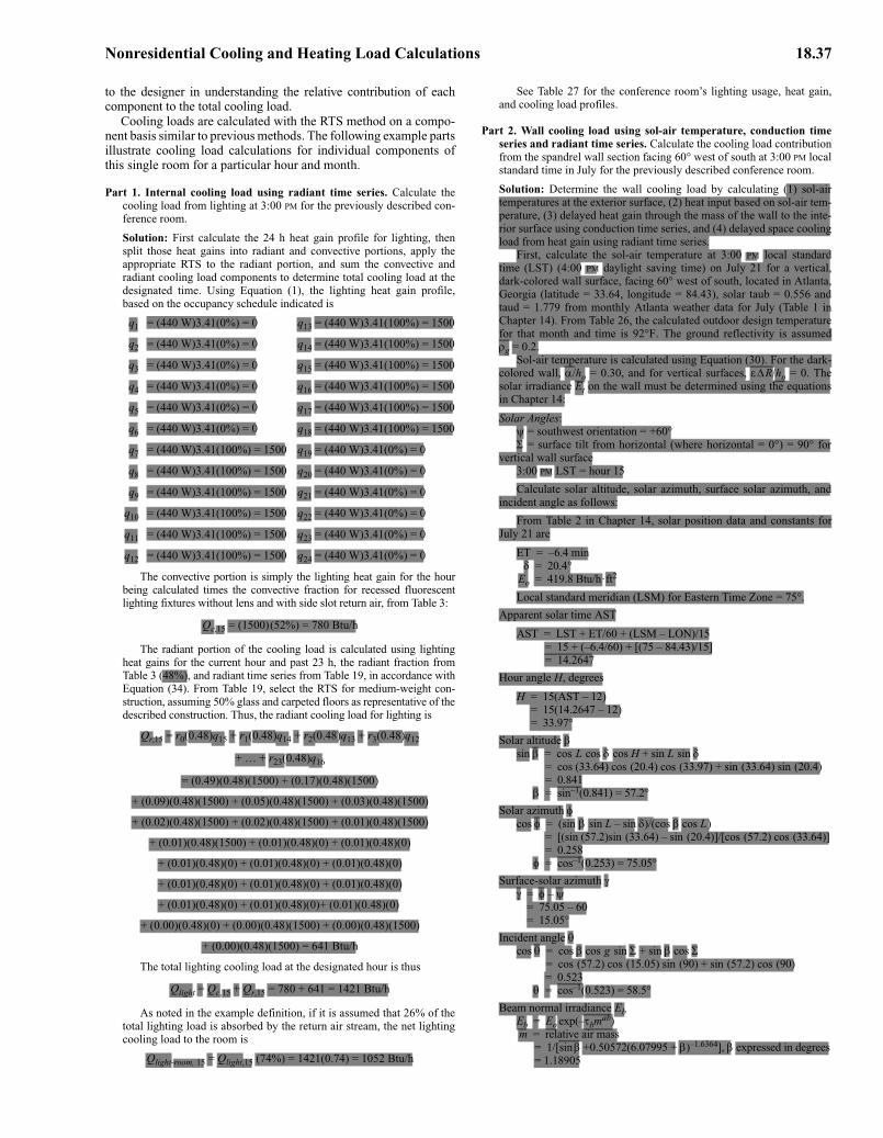
Nonresidential Cooling and Heating Load Calculations 18.37

to the designer in understanding the relative contribution of eachcomponent to the total cooling load.

Cooling loads are calculated with the RTS method on a compo-nent basis similar to previous methods. The following example partsillustrate cooling load calculations for individual components ofthis single room for a particular hour and month.

Part 1. Internal cooling load using radiant time series. Calculate thecooling load from lighting at 3:00 PM for the previously described con-ference room.

Solution: First calculate the 24 h heat gain profile for lighting, thensplit those heat gains into radiant and convective portions, apply theappropriate RTS to the radiant portion, and sum the convective andradiant cooling load components to determine total cooling load at thedesignated time. Using Equation (1), the lighting heat gain profile,based on the occupancy schedule indicated is

q1 = (440 W)3.41(0%) = 0 q13 = (440 W)3.41(100%) = 1500

q2 = (440 W)3.41(0%) = 0 q14 = (440 W)3.41(100%) = 1500

q3 = (440 W)3.41(0%) = 0 q15 = (440 W)3.41(100%) = 1500

q4 = (440 W)3.41(0%) = 0 q16 = (440 W)3.41(100%) = 1500

q5 = (440 W)3.41(0%) = 0 q17 = (440 W)3.41(100%) = 1500

q6 = (440 W)3.41(0%) = 0 q18 = (440 W)3.41(100%) = 1500

q7 = (440 W)3.41(100%) = 1500 q19 = (440 W)3.41(0%) = 0

q8 = (440 W)3.41(100%) = 1500 q20 = (440 W)3.41(0%) = 0

q9 = (440 W)3.41(100%) = 1500 q21 = (440 W)3.41(0%) = 0

q10 = (440 W)3.41(100%) = 1500 q22 = (440 W)3.41(0%) = 0

q11 = (440 W)3.41(100%) = 1500 q23 = (440 W)3.41(0%) = 0

q12 = (440 W)3.41(100%) = 1500 q24 = (440 W)3.41(0%) = 0

The convective portion is simply the lighting heat gain for the hourbeing calculated times the convective fraction for recessed fluorescentlighting fixtures without lens and with side slot return air, from Table 3:

Qc,15 = (1500)(52%) = 780 Btu/h

The radiant portion of the cooling load is calculated using lightingheat gains for the current hour and past 23 h, the radiant fraction fromTable 3 (48%), and radiant time series from Table 19, in accordance withEquation (34). From Table 19, select the RTS for medium-weight con-struction, assuming 50% glass and carpeted floors as representative of thedescribed construction. Thus, the radiant cooling load for lighting is

Qr,15 = r0(0.48)q15 + r1(0.48)q14 + r2(0.48)q13 + r3(0.48)q12

+ … + r23(0.48)q16

= (0.49)(0.48)(1500) + (0.17)(0.48)(1500)

+ (0.09)(0.48)(1500) + (0.05)(0.48)(1500) + (0.03)(0.48)(1500)

+ (0.02)(0.48)(1500) + (0.02)(0.48)(1500) + (0.01)(0.48)(1500)

+ (0.01)(0.48)(1500) + (0.01)(0.48)(0) + (0.01)(0.48)(0)

+ (0.01)(0.48)(0) + (0.01)(0.48)(0) + (0.01)(0.48)(0)

+ (0.01)(0.48)(0) + (0.01)(0.48)(0) + (0.01)(0.48)(0)

+ (0.01)(0.48)(0) + (0.01)(0.48)(0)+ (0.01)(0.48)(0)

+ (0.00)(0.48)(0) + (0.00)(0.48)(1500) + (0.00)(0.48)(1500)

+ (0.00)(0.48)(1500) = 641 Btu/h

The total lighting cooling load at the designated hour is thus

Qlight = Qc,15 + Qr,15 = 780 + 641 = 1421 Btu/h

As noted in the example definition, if it is assumed that 26% of thetotal lighting load is absorbed by the return air stream, the net lightingcooling load to the room is

Qlight-room, 15 = Qlight,15 (74%) = 1421(0.74) = 1052 Btu/h

See Table 27 for the conference room’s lighting usage, heat gain,and cooling load profiles.

Part 2. Wall cooling load using sol-air temperature, conduction timeseries and radiant time series. Calculate the cooling load contributionfrom the spandrel wall section facing 60° west of south at 3:00 PM localstandard time in July for the previously described conference room.

Solution: Determine the wall cooling load by calculating (1) sol-airtemperatures at the exterior surface, (2) heat input based on sol-air tem-perature, (3) delayed heat gain through the mass of the wall to the inte-rior surface using conduction time series, and (4) delayed space coolingload from heat gain using radiant time series.

First, calculate the sol-air temperature at 3:00 PM local standardtime (LST) (4:00 PM daylight saving time) on July 21 for a vertical,dark-colored wall surface, facing 60° west of south, located in Atlanta,Georgia (latitude = 33.64, longitude = 84.43), solar taub = 0.556 andtaud = 1.779 from monthly Atlanta weather data for July (Table 1 inChapter 14). From Table 26, the calculated outdoor design temperaturefor that month and time is 92°F. The ground reflectivity is assumedρg = 0.2.

Sol-air temperature is calculated using Equation (30). For the dark-colored wall, α/ho = 0.30, and for vertical surfaces, εΔR/ho = 0. Thesolar irradiance Et on the wall must be determined using the equationsin Chapter 14:

Solar Angles:ψ = southwest orientation = +60°Σ = surface tilt from horizontal (where horizontal = 0°) = 90° for

vertical wall surface3:00 PM LST = hour 15

Calculate solar altitude, solar azimuth, surface solar azimuth, andincident angle as follows:

From Table 2 in Chapter 14, solar position data and constants forJuly 21 are

ET = –6.4 minδ = 20.4°

Eo = 419.8 Btu/h·ft2

Local standard meridian (LSM) for Eastern Time Zone = 75°.

Apparent solar time AST

AST = LST + ET/60 + (LSM – LON)/15 = 15 + (–6.4/60) + [(75 – 84.43)/15]

= 14.2647

Hour angle H, degrees

H = 15(AST – 12) = 15(14.2647 – 12) = 33.97°

Solar altitude βsin β = cos L cos δ cos H + sin L sin δ

= cos (33.64) cos (20.4) cos (33.97) + sin (33.64) sin (20.4)= 0.841

β = sin–1(0.841) = 57.2°

Solar azimuth φcos φ = (sin β sin L – sin δ)/(cos β cos L)

= [(sin (57.2)sin (33.64) – sin (20.4)]/[cos (57.2) cos (33.64)]= 0.258

φ = cos–1(0.253) = 75.05°

Surface-solar azimuth γγ = φ – ψ = 75.05 – 60 = 15.05°

Incident angle θcos θ = cos β cos g sin Σ + sin β cos Σ

= cos (57.2) cos (15.05) sin (90) + sin (57.2) cos (90)= 0.523

θ = cos–1(0.523) = 58.5°

Beam normal irradiance EbEb = Eo exp(–τbmab)m = relative air mass

= 1/[sin β +0.50572(6.07995 + β)–1.6364], β expressed in degrees= 1.18905

18.38 2009 ASHRAE Handbook—Fundamentals

Table 26 Monthly/Hourly Design Temperatures (5% Conditions) for Atlanta, GA, °FJanuary February March April May June July August September October November December

Hour db wb db wb db wb db wb db wb db wb db wb db wb db wb db wb db wb db wb

1 44.1 43.0 47.2 45.9 52.8 48.3 59.2 54.2 66.3 61.9 71.3 66.3 73.8 68.9 73.2 68.9 69.4 65.4 60.9 57.6 53.3 51.8 47.1 46.92 43.3 42.5 46.4 45.4 51.9 47.9 58.2 53.8 65.5 61.6 70.4 66.0 73.0 68.6 72.5 68.7 68.6 65.1 60.1 57.3 52.5 51.3 46.3 46.33 42.6 42.0 45.8 45.0 51.2 47.5 57.6 53.5 64.9 61.4 69.8 65.8 72.3 68.4 71.9 68.5 68.0 64.9 59.5 57.0 51.9 51.0 45.7 45.74 42.0 41.6 45.1 44.7 50.5 47.1 56.9 53.2 64.3 61.2 69.2 65.6 71.7 68.2 71.3 68.3 67.5 64.7 58.9 56.8 51.3 50.6 45.1 45.15 41.6 41.3 44.7 44.4 50.0 46.9 56.4 53.0 63.9 61.0 68.8 65.5 71.3 68.1 70.9 68.2 67.1 64.6 58.5 56.6 50.9 50.4 44.7 44.76 42.0 41.6 45.1 44.7 50.5 47.1 56.9 53.2 64.3 61.2 69.2 65.6 71.7 68.2 71.3 68.3 67.5 64.7 58.9 56.8 51.3 50.6 45.1 45.17 43.5 42.6 46.6 45.6 52.1 48.0 58.5 53.9 65.7 61.7 70.6 66.1 73.2 68.7 72.6 68.7 68.8 65.2 60.3 57.4 52.7 51.4 46.5 46.58 47.0 45.1 50.2 47.8 56.1 50.0 62.4 55.5 69.2 63.1 74.1 67.2 76.7 69.7 75.9 69.8 72.0 66.3 63.6 58.9 56.2 53.4 49.8 48.89 51.0 47.8 54.2 50.2 60.5 52.3 66.8 57.4 73.1 64.6 78.0 68.5 80.6 70.9 79.6 70.9 75.6 67.6 67.4 60.5 60.0 55.6 53.5 51.3

10 54.5 50.3 57.8 52.4 64.4 54.3 70.7 59.1 76.5 65.9 81.5 69.6 84.1 72.0 82.9 72.0 78.8 68.8 70.7 62.0 63.4 57.5 56.9 53.611 57.6 52.5 61.0 54.3 67.9 56.1 74.1 60.5 79.6 67.1 84.6 70.6 87.2 73.0 85.8 72.9 81.7 69.8 73.7 63.3 66.5 59.3 59.8 55.612 59.7 53.9 63.1 55.6 70.3 57.3 76.4 61.5 81.6 67.9 86.6 71.2 89.3 73.6 87.8 73.5 83.5 70.4 75.6 64.2 68.5 60.4 61.8 57.013 61.4 55.1 64.8 56.7 72.1 58.2 78.3 62.3 83.3 68.5 88.3 71.8 91.0 74.1 89.3 74.0 85.1 71.0 77.2 64.9 70.1 61.3 63.3 58.014 62.4 55.8 65.9 57.3 73.3 58.8 79.4 62.8 84.3 68.9 89.3 72.1 92.0 74.4 90.3 74.3 86.0 71.3 78.2 65.3 71.1 61.9 64.3 58.715 62.4 55.8 65.9 57.3 73.3 58.8 79.4 62.8 84.3 68.9 89.3 72.1 92.0 74.4 90.3 74.3 86.0 71.3 78.2 65.3 71.1 61.9 64.3 58.716 61.2 54.9 64.6 56.5 71.9 58.1 78.0 62.2 83.1 68.4 88.1 71.7 90.8 74.0 89.1 73.9 84.9 70.9 77.0 64.8 69.9 61.2 63.1 57.917 59.5 53.8 62.9 55.5 70.0 57.1 76.2 61.4 81.4 67.8 86.4 71.2 89.1 73.5 87.6 73.4 83.4 70.4 75.4 64.1 68.3 60.3 61.6 56.818 57.4 52.3 60.8 54.2 67.7 55.9 73.9 60.4 79.4 67.0 84.4 70.5 87.0 72.9 85.6 72.8 81.5 69.7 73.5 63.2 66.3 59.1 59.6 55.519 54.3 50.1 57.6 52.3 64.2 54.2 70.4 59.0 76.3 65.8 81.3 69.5 83.9 71.9 82.7 71.9 78.6 68.7 70.5 61.9 63.2 57.4 56.7 53.520 52.0 48.6 55.3 50.9 61.7 52.9 67.9 57.9 74.1 65.0 79.1 68.8 81.7 71.3 80.6 71.3 76.6 68.0 68.4 61.0 61.0 56.2 54.5 52.021 50.1 47.2 53.4 49.7 59.6 51.8 65.8 57.0 72.3 64.2 77.2 68.2 79.8 70.7 78.9 70.7 74.8 67.3 66.6 60.2 59.2 55.1 52.7 50.822 48.3 45.9 51.5 48.5 57.5 50.7 63.8 56.1 70.4 63.5 75.4 67.6 77.9 70.1 77.1 70.2 73.1 66.7 64.8 59.4 57.4 54.1 51.0 49.623 46.6 44.8 49.8 47.5 55.6 49.8 61.9 55.4 68.8 62.9 73.7 67.1 76.3 69.6 75.6 69.7 71.6 66.2 63.2 58.7 55.7 53.2 49.4 48.524 45.3 43.9 48.5 46.7 54.2 49.0 60.5 54.8 67.6 62.4 72.5 66.7 75.0 69.2 74.4 69.3 70.5 65.8 62.0 58.2 54.5 52.5 48.2 47.7

Table 27 Cooling Load Component: Lighting, Btu/h

Hour

UsageProfile,

%

Heat Gain, Btu/hNonsolar RTS Zone Type 8,

%

Radiant Cooling

Load

TotalSensible

Cooling Load

% Lightingto Return

26%

RoomSensible

Cooling LoadConvective Radiant

Total 52% 48%

1 0 — — — 49 86 86 22 642 0 — — — 17 86 86 22 643 0 — — — 9 79 79 21 594 0 — — — 5 72 72 19 535 0 — — — 3 65 65 17 486 0 — — — 2 58 58 15 437 100 1,500 780 720 2 403 1,184 308 8768 100 1,500 780 720 1 519 1,299 338 9619 100 1,500 780 720 1 576 1,356 353 1,004

10 100 1,500 780 720 1 605 1,385 360 1,02511 100 1,500 780 720 1 619 1,400 364 1,03612 100 1,500 780 720 1 627 1,407 366 1,04113 100 1,500 780 720 1 634 1,414 368 1,04614 100 1,500 780 720 1 634 1,414 368 1,04615 100 1,500 780 720 1 641 1,421 370 1,05216 100 1,500 780 720 1 648 1,428 371 1,05717 100 1,500 780 720 1 655 1,436 373 1,06218 100 1,500 780 720 1 663 1,443 375 1,06819 0 — — — 1 317 317 82 23420 0 — — — 1 202 202 52 14921 0 — — — 0 144 144 37 10722 0 — — — 0 115 115 30 8523 0 — — — 0 101 101 26 7524 0 — — — 0 94 94 24 69

Total 18,005 9,362 8,642 1 8,642 18,005 4,681 13,324

Nonresidential Cooling and Heating Load Calculations 18.39

ab = beam air mass exponent= 1.219 – 0.043τb – 0.151τd – 0.204τbτd= 0.72468

Eb = 419.8 exp[–0.556(1.89050.72468)]= 223.5 Btu/h·ft2

Surface beam irradiance Et,bEt,b = Eb cos θ

= (223.5) cos (58.5) = 117 Btu/h·ft2

Ratio Y of sky diffuse radiation on vertical surface to sky diffuse radia-tion on horizontal surface

Y = 0.55 + 0.437 cos θ + 0.313 cos2θ= 0.55 + 0.437 cos (58.5) + 0.313 cos2(58.5)= 0.864

Diffuse irradiance Ed – Horizontal surfacesEd = Eo exp(–τdmad)ad = diffuse air mass exponent

= 0.202 + 0.852τb – 0.007τd – 0.357τbτd= 0.3101417

Ed = Eo exp(–τdmad)= 419.8 exp(–1.779(1.89050.3101)]= 64.24 Btu/h·ft2

Diffuse irradiance Ed – Vertical surfacesEt,d = EdY

= (64.24)(0.864)= 55.5 Btu/h·ft2

Ground reflected irradiance Et,rEt,r = (Eb sin β + Ed)ρg(l – cos Σ)/2

= [223.5 sin (57.2) + 64.24](0.2)[1 – cos (90)]/2= 25.2 Btu/h·ft2

Total surface irradiance EtEt = ED + Ed + Er

= 117 + 55.5 + 25.2= 197.7 Btu/h·ft2

Sol–air temperature [from Equation (30)]:Te = to + αEt /ho – εΔR/ho = 92 + (0.30)(197.7) – 0 = 151°F

This procedure is used to calculate the sol-air temperatures for eachhour on each sur face. Because of th e tedious solar angle and intensitycalculations, using a simple comput er spr eadsheet or othe r compute rsoftware can reduce the effort involved. A spreadsheet was used to cal-culate a 24 h sol- air temperature profile for the data of this e xample.See Table 28A for the solar angle and intensity calculations and Table28B for the sol-air temperatures for this wall surface and orientation.

Conductive heat gain is calculated using Equations (31) and (32).First, calculate the 24 h heat inpu t profile using Equation (31) and thesol-air tempe ratures for a southwes t-facing w all with dark e xteriorcolor:

qi,1 = (0.08)(120)(73.8 – 75) = –12 Btu/hqi,2 = (0.08)(120)(73 – 75) = –19qi,3 = (0.08)(120)(72.3 – 75) = –26qi,4 = (0.08)(120)(71.7 – 75) = –32qi,5 = (0.08)(120)(71.3 – 75) = –36qi,6 = (0.08)(120)(72.7 – 75) = –22qi,7 = (0.08)(120)(78.4 – 75) = 33qi,8 = (0.08)(120)(85.9 – 75) = 104qi,9 = (0.08)(120)(93.1 – 75) = 174

qi,10 = (0.08)(120)(99.3 – 75) = 234qi,11 = (0.08)(120)(104.5 – 75) = 283qi,12 = (0.08)(120)(109.2 – 75) = 328qi,13 = (0.08)(120)(125.4 – 75) = 484qi,14 = (0.08)(120)(141.4 – 75) = 638qi,15 = (0.08)(120)(151.3 – 75) = 733qi,16 = (0.08)(120)(152.7 – 75) = 746qi,17 = (0.08)(120)(144.8 – 75) = 670qi,18 = (0.08)(120)(126.6 – 75) = 495qi,19 = (0.08)(120)(98 – 75) = 221qi,20 = (0.08)(120)(81.7 – 75) = 064qi,21 = (0.08)(120)(79.8 – 75) = 046qi,22 = (0.08)(120)(77.9 – 75) = 028

qi,23 = (0.08)(120)(76.3 – 75) = 12qi,24 = (0.08)(120)(75 – 75) = 00

Next, c alculate w all heat gain using conduction time ser ies. Thepreceding heat input profile is used with conduction time series to cal-culate the w all heat gain. From T able 16, the most simila r wall con-struction is wall number 1. This is a spandrel glass wall that has similarmass and thermal capacity . Using Eq uation (32), the c onduction timefactors for wall 1 ca n be used in co njunction with the 24 h heat inputprofile to determine the wall heat gain at 3:00 PM LST:

q15 = c0qi,15 + c1qi,14 + c2qi,13 + c3qi,12 + … + c23qi,14= (0.18)(733) + (0.58)(638) + (0.20)(484) + (0.04)(328)

+ (0.00)(283) + (0.00)(234) + (0.00)(174) + (0.00)(104)+ (0.00)(33) + (0.00)(–22) + (0.00)(–36) + (0.00)(–32)+ (0.00)(–26) + (0.00)(–19) + (0.00)(–12) + (0.00)(0)+ (0.00)(12) + (0.00)(28) + (0.00)(46) + (0.00)(64)+ (0.00)(221) + (0.00)(495) + (0.00)(670) + (0.00)(746)

= 612 Btu/h

Because of the tedious calculations involved, a spreadsheet is usedto calculate the remainder of a 24 h heat gain profile indicated in Table28B for the data of this example.

Finally, calculate wall cooling load using radiant time ser ies. Totalcooling load for the wall is calculated by summing the convective andradiant portions. The convective portion is simply the wall heat gain forthe hour being calculated times th e convective fraction for walls fromTable 14 (54%):

Qc = (612)(0.54) = 330 Btu/h

The radiant portion of the cooling load is calculated using conduc-tive hea t gains f or the curre nt a nd past 2 3 h, the r adiant fr action f orwalls from Table 14 (46%), and radiant time ser ies from Table 19, inaccordance w ith E quation (34) . Fr om T able 19, select the R TS formedium-weight construction, assuming 50% glass and car peted floorsas representative for the described construction. Use the wall heat gainsfrom Table 28B for 24 h design conditions in July. Thus, the radiantcooling load for the wall at 3:00 PM is

Qr,15 = r0(0.46)qi,15 + r1(0.46) qi,14 + r2(0.46) qi,13 + r3(0.46) qi,12+ … + r23(0.46) qi,16

= (0.49)(0.46)(612) + (0.17)(0.46)(472) + (0.09)(0.46)(344)+ (0.05)(0.46)(277) + (0.03)(0.46)(225) + (0.02)(0.46)(165)+ (0.02)(0.46)(97) + (0.01)(0.46)(32) + (0.01)(0.46)(–15)+ (0.01)(0.46)(–32) + (0.01)(0.46)(–31) + (0.01)(0.46)(–25)+ (0.01)(0.46)(–18) + (0.01)(0.46)(–10) + (0.01)(0.46)(2) + (0.01)(0.46)(15) + (0.01)(0.46)(30) + (0.01)(0.46)(53) + (0.01)(0.46)(110) + (0.01)(0.46)(266) + (0.00)(0.46)(491)+ (0.00)(0.46)(656) + (0.00)(0.46)(725) + (0.00)(0.46)(706)

= 203 Btu/h

The total wall cooling load at the designated hour is thus

Qwall = Qc + Qr15 = 330 + 203 = 533 Btu/h

Again, a simple computer spreadsheet or other sof tware is ne ces-sary to reduce the effort involved. A spreadsheet was used with the heatgain profile to split the heat gain into convective and radiant portions,apply RTS to th e radiant portion, and total the con vective and ra diantloads to dete rmine a 24 h cooling load profile for this e xample, withresults in Table 28B.

Part 3. Window co oling load using radiant t ime series. Calc ulate thecooling load contribution, with an d without inside s hading (venetianblinds) for the window area facing 60° west of south at 3:00 PM in Julyfor the conference room example.

Solution: First, calculate the 24 h heat gain profile for the window, thensplit those heat gains into r adiant and c onvective portions, apply theappropriate RTS to the radiant por tion, then sum the con vective andradiant cooling load components to determine total windo w c oolingload for the time. T he windo w he at gain components ar e calculatedusing Equations (13) to (15). From Part 2, at hour 15 LST (3:00 PM):

Et,b = 117 Btu/h·ft2Et,d = 55.5 Btu/h·ft2Er = 25.2 Btu/h·ft2θ = 58.5°

18.40 2009 ASHRAE Handbook—Fundamentals

Table 28A Wall Component of Solar Irradiance

Local Standard

Hour

Apparent Solar Time

Hour Angle

H

Solar Altitude

β

Solar Azimuth

ϕ

Direct Beam Solar Diffuse Solar Heat Gain Total Surface

Irradiance Btu/h·ft2

Eb , Direct Normal

Btu/h·ft2

Surface Incident Angle θ

Surface Direct

Btu/h·ft2

Ed, Diffuse Horizontal,

Btu/h·ft2

Ground Diffuse

Btu/h·ft2 Y

Ratio

SkyDiffuse

Btu/h·ft2

Subtotal Diffuse

Btu/h·ft2

1 0.26 –176 –36 –175 0.0 117.4 0.0 0.0 0.0 0.4500 0.0 0.0 0.02 1.26 –161 –33 –159 0.0 130.9 0.0 0.0 0.0 0.4500 0.0 0.0 0.03 2.26 –146 –27 –144 0.0 144.5 0.0 0.0 0.0 0.4500 0.0 0.0 0.04 3.26 –131 –19 –132 0.0 158.1 0.0 0.0 0.0 0.4500 0.0 0.0 0.05 4.26 –116 –9 –122 0.0 171.3 0.0 0.0 0.0 0.4500 0.0 0.0 0.06 5.26 –101 3 –113 5.6 172.5 0.0 5.8 0.6 0.4500 2.6 3.2 3.27 6.26 –86 14 –105 92.4 159.5 0.0 27.4 5.0 0.4500 12.3 17.3 17.38 7.26 –71 27 –98 155.4 145.9 0.0 42.9 11.2 0.4500 19.3 30.5 30.59 8.26 –56 39 –90 193.1 132.3 0.0 53.9 17.5 0.4500 24.3 41.8 41.8

10 9.26 –41 51 –81 216.1 118.8 0.0 61.6 23.1 0.4500 27.7 50.8 50.811 10.26 –26 63 –67 229.8 105.6 0.0 66.6 27.2 0.4553 30.3 57.5 57.512 11.26 –11 74 –39 236.7 92.6 0.0 69.3 29.6 0.5306 36.8 66.4 66.413 12.26 4 76 16 238.0 80.2 40.4 69.8 30.1 0.6332 44.2 74.3 114.714 13.26 19 69 57 233.8 68.7 85.1 68.1 28.6 0.7505 51.1 79.7 164.815 14.26 34 57 75 223.5 58.4 117.0 64.2 25.2 0.8644 55.5 80.7 197.716 15.26 49 45 86 205.3 50.4 130.8 57.9 20.3 0.9555 55.3 75.6 206.417 16.26 64 32 94 175.5 45.8 122.4 48.5 14.3 1.0073 48.9 63.2 185.618 17.26 79 20 102 126.2 45.5 88.4 35.4 7.9 1.0100 35.7 43.6 132.019 18.26 94 8 109 44.7 49.7 28.9 16.6 2.3 0.9631 16.0 18.3 47.120 19.26 109 –3 117 0.0 57.5 0.0 0.0 0.0 0.8755 0.0 0.0 0.021 20.26 124 –14 127 0.0 67.5 0.0 0.0 0.0 0.7630 0.0 0.0 0.022 21.26 139 –23 138 0.0 79.0 0.0 0.0 0.0 0.6452 0.0 0.0 0.023 22.26 154 –30 151 0.0 91.3 0.0 0.0 0.0 0.5403 0.0 0.0 0.024 23.26 169 –35 167 0.0 104.2 0.0 0.0 0.0 0.4618 0.0 0.0 0.0

Table 28B Wall Component of Sol-Air Temperatures, Heat Input, Heat Gain, Cooling Load

Local Standard

Hour

Total Surface

Irradiance Btu/h·ft2

Outside Temp.,

°F

Sol-Air Temp.,

°F

Inside Temp.,

°F

Heat Input, Btu/h

CTSType 1,

%

Heat Gain, Btu/h Nonsolar RTS Zone

Type 8,%

Radiant Cooling Load, Btu/h

Total Cooling Load, Btu/h

Convective Radiant

Total 54% 46%

1 0.0 73.8 74 75 –12 18 2 1 1 49 32 332 0.0 73.0 73 75 –19 58 –10 –5 –4 17 25 203 0.0 72.3 72 75 –26 20 –18 –10 –8 9 21 114 0.0 71.7 72 75 –32 4 –25 –14 –12 5 17 45 0.0 71.3 71 75 –36 0 –31 –17 –14 3 14 –36 3.2 71.7 73 75 –22 0 –32 –17 –15 2 12 –57 17.3 73.2 78 75 33 0 –15 –8 –7 2 14 58 30.5 76.7 86 75 104 0 32 17 15 1 24 419 41.8 80.6 93 75 174 0 97 53 45 1 41 94

10 50.8 84.1 99 75 234 0 165 89 76 1 62 15111 57.5 87.2 104 75 283 0 225 122 104 1 81 20312 66.4 89.3 109 75 328 0 277 149 127 1 100 24913 114.7 91.0 125 75 484 0 344 185 158 1 121 30614 164.8 92.0 141 75 638 0 472 255 217 1 157 41215 197.7 92.0 151 75 733 0 612 330 281 1 203 53316 206.4 90.8 153 75 746 0 706 381 325 1 243 62417 185.6 89.1 145 75 670 0 725 392 334 1 265 65718 132.0 87.0 127 75 495 0 656 354 302 1 262 61719 47.1 83.9 98 75 221 0 491 265 226 1 227 49220 0.0 81.7 82 75 64 0 266 143 122 1 167 31021 0.0 79.8 80 75 46 0 110 59 50 0 110 16922 0.0 77.9 78 75 28 0 53 29 25 0 75 10423 0.0 76.3 76 75 12 0 30 16 14 0 54 7024 0.0 75.0 75 75 0 0 15 8 7 0 41 49

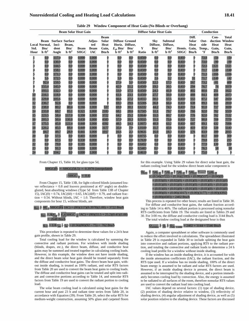
Nonresidential Cooling and Heating Load Calculations 18.41

From Chapter 15, Table 10, for glass type 5d,

SHGC(θ) = SHGC(58.5) = 0.3978 (interpolated)

⟨SHGC⟩D = 0.41

From Chapter 15, Table 13B, for light-colored blinds (assumed lou-ver reflectance = 0.8 and louvers positioned at 45° angle) on double-glazed, heat-absorbing windows (Type 5d from Table 13B of Chapter15), IAC(0) = 0.74, IAC(60) = 0.65, IAC(diff) = 0.79, and radiant frac-tion = 0.54. Without blinds, IAC = 1.0. Therefore, window heat gaincomponents for hour 15, without blinds, are

qb15 = AEt,b SHGC(θ)(IAC) = (80)(117)(0.3978)(1.00) = 3722 Btu/h

qd15 = A(Et,d + Er)⟨SHGC⟩D(IAC) = (80)(55.5 + 25.2)(0.41)(1.00)= 2648 Btu/h

qc15 = UA(tout – tin) = (0.56)(80)(92 – 75) = 762 Btu/h

This procedure is repeated to determine these values for a 24 h heatgain profile, shown in Table 29.

Total cooling load for the window is calculated by summing theconvective and radiant portions. For windows with inside shading(blinds, drapes, etc.), the direct beam, diffuse, and conductive heatgains may be summed and treated together in calculating cooling loads.However, in this example, the window does not have inside shading,and the direct beam solar heat gain should be treated separately fromthe diffuse and conductive heat gains. The direct beam heat gain, with-out inside shading, is treated as 100% radiant, and solar RTS factorsfrom Table 20 are used to convert the beam heat gains to cooling loads.The diffuse and conductive heat gains can be totaled and split into radi-ant and convective portions according to Table 14, and nonsolar RTSfactors from Table 19 are used to convert the radiant portion to coolingload.

The solar beam cooling load is calculated using heat gains for thecurrent hour and past 23 h and radiant time series from Table 20, inaccordance with Equation (39). From Table 20, select the solar RTS formedium-weight construction, assuming 50% glass and carpeted floors

for this example. Using Table 29 values for direct solar heat gain, theradiant cooling load for the window direct beam solar component is

Qb,15 = r0qb,15 + r1qb,14 + r2qb,13 + r3qb,12 + … + r23qb,14

= (0.54)(3722) + (0.16)(2183) + (0.08)(537) + (0.04)(0)+ (0.03)(0) + (0.02)(0) + (0.01)(0) + (0.01)(0) + (0.01)(0)+ (0.01)(0) + (0.01)(0) + (0.01)(0) + (0.01)(0) + (0.01)(0)+ (0.01)(0) + (0.01)(0) + (0.01)(0) + (0.01)(0) + (0.01)(0)+ (0.00)(0) + (0.00)(1017) + (0.00)(3177) + (0.00)(4392)+ (0.00)(4583) = 2402 Btu/h

This process is repeated for other hours; results are listed in Table 30.For diffuse and conductive heat gains, the radiant fraction accord-

ing to Table 14 is 46%. The radiant portion is processed using nonsolarRTS coefficients from Table 19. The results are listed in Tables 29 and30. For 3:00 PM, the diffuse and conductive cooling load is 3144 Btu/h.

The total window cooling load at the designated hour is thus

Qwindow = Qb + Qdiff + cond = 2402 + 3144 = 5546 Btu/h

Again, a computer spreadsheet or other software is commonly usedto reduce the effort involved in calculations. The spreadsheet illustratedin Table 29 is expanded in Table 30 to include splitting the heat gaininto convective and radiant portions, applying RTS to the radiant por-tion, and totaling the convective and radiant loads to determine a 24 hcooling load profile for a window without inside shading.

If the window has an inside shading device, it is accounted for withthe inside attenuation coefficients (IAC), the radiant fraction, and theRTS type used. If a window has no inside shading, 100% of the directbeam energy is assumed to be radiant and solar RTS factors are used.However, if an inside shading device is present, the direct beam isassumed to be interrupted by the shading device, and a portion immedi-ately becomes cooling load by convection. Also, the energy is assumedto be radiated to all surfaces of the room, therefore nonsolar RTS valuesare used to convert the radiant load into cooling load.

IAC values depend on several factors: (1) type of shading device,(2) position of shading device relative to window, (3) reflectivity ofshading device, (4) angular adjustment of shading device, as well as (5)solar position relative to the shading device. These factors are discussed

Table 29 Window Component of Heat Gain (No Blinds or Overhang)

Local Std.

Hour

Beam Solar Heat Gain Diffuse Solar Heat Gain Conduction

Total Window

Heat Gain, Btu/h

Beam Normal,

Btu/h·ft2

Surface Inci-dent

Angle

Surface Beam, Btu/h·ft2

Beam SHGC

Adjus-ted

Beam IAC

Beam SolarHeat Gain, Btu/h

Diffuse Horiz.

Ed, Btu/h·ft2

Ground Diffuse,

Btu/h·ft2

YRatio

Sky Diffuse,

Btu/h·ft2

Subtotal Diffuse,

Btu/h·ft2

Hemis. SHGC

Diff. Solar Heat Gain, Btu/h

Out-side

Temp.,°F

Con-duction

Heat Gain, Btu/h

1 0.0 117.4 0.0 0.000 1.000 0 0.0 0.0 0.4500 0.0 0.0 0.410 0 73.8 –54 –542 0.0 130.9 0.0 0.000 1.000 0 0.0 0.0 0.4500 0.0 0.0 0.410 0 73.0 –90 –903 0.0 144.5 0.0 0.000 1.000 0 0.0 0.0 0.4500 0.0 0.0 0.410 0 72.3 –121 –1214 0.0 158.1 0.0 0.000 1.000 0 0.0 0.0 0.4500 0.0 0.0 0.410 0 71.7 –148 –1485 0.0 171.3 0.0 0.000 1.000 0 0.0 0.0 0.4500 0.0 0.0 0.410 0 71.3 –166 –1666 5.6 172.5 0.0 0.000 0.000 0 5.8 0.6 0.4500 2.6 3.2 0.410 31 71.7 –148 –427 92.4 159.5 0.0 0.000 0.000 0 27.4 5.0 0.4500 12.3 17.3 0.410 167 73.2 –81 4888 155.4 145.9 0.0 0.000 0.000 0 42.9 11.2 0.4500 19.3 30.5 0.410 294 76.7 76 10789 193.1 132.3 0.0 0.000 0.000 0 53.9 17.5 0.4500 24.3 41.8 0.410 402 80.6 251 162210 216.1 118.8 0.0 0.000 0.000 0 61.6 23.1 0.4500 27.7 50.8 0.410 488 84.1 408 207311 229.8 105.6 0.0 0.000 0.000 0 66.6 27.2 0.4553 30.3 57.5 0.410 553 87.2 547 243412 236.7 92.6 0.0 0.000 0.000 0 69.3 29.6 0.5306 36.8 66.4 0.410 638 89.3 641 281813 238.0 80.2 40.4 0.166 1.000 537 69.8 30.1 0.6332 44.2 74.3 0.410 714 91.0 717 369014 233.8 68.7 85.1 0.321 1.000 2183 68.1 28.6 0.7505 51.1 79.7 0.410 766 92.0 762 555915 223.5 58.4 117.0 0.398 1.000 3722 64.2 25.2 0.8644 55.5 80.7 0.410 776 92.0 762 713216 205.3 50.4 130.8 0.438 1.000 4583 57.9 20.3 0.9555 55.3 75.6 0.410 727 90.8 708 777017 175.5 45.8 122.4 0.448 1.000 4392 48.5 14.3 1.0073 48.9 63.2 0.410 607 89.1 632 709618 126.2 45.5 88.4 0.449 1.000 3177 35.4 7.9 1.0100 35.7 43.6 0.410 419 87.0 538 514319 44.7 49.7 28.9 0.441 1.000 1017 16.6 2.3 0.9631 16.0 18.3 0.410 176 83.9 399 201520 0.0 57.5 0.0 0.403 0.000 0 0.0 0.0 0.8755 0.0 0.0 0.410 0 81.7 300 30021 0.0 67.5 0.0 0.330 0.000 0 0.0 0.0 0.7630 0.0 0.0 0.410 0 79.8 215 21522 0.0 79.0 0.0 0.185 0.000 0 0.0 0.0 0.6452 0.0 0.0 0.410 0 77.9 130 13023 0.0 91.3 0.0 0.000 1.000 0 0.0 0.0 0.5403 0.0 0.0 0.410 0 76.3 58 5824 0.0 104.2 0.0 0.000 1.000 0 0.0 0.0 0.4618 0.0 0.0 0.410 0 75.0 0 0

18.42 2009 ASHRAE Handbook—Fundamentals

in detail in Chapter 15. For this example with venetian blinds, the IACfor beam radiation is treated separately from the diffuse solar gain. Thedirect beam IAC must be adjusted based on the profile angle of the sun.At 3:00 PM in July, the profile angle of the sun relative to the windowsurface is 58°. Calculated using Equation (45) from Chapter 15, thebeam IAC = 0.653. The diffuse IAC is 0.79. Thus, the window heatgains, with light-colored blinds, at 3:00 PM are

qb15 = AED SHGC(θ)(IAC) = (80)(117)(0.3978)(0.653) = 2430 Btu/h

qd15 = A(Ed + Er)⟨SHGC⟩D(IAC)D= (80)(55.5 + 25.2)(0.41)(0.79)= 2092 Btu/h

qc15 = UA(tout – tin) = (0.56)(80)(92 – 75) = 762 Btu/h

Because the same radiant fraction and nonsolar RTS are applied toall parts of the window heat gain when inside shading is present, thoseloads can be totaled and the cooling load calculated after splitting theradiant portion for processing with nonsolar RTS. This is illustrated bythe spreadsheet results in Table 31. The total window cooling load withvenetian blinds at 3:00 PM = 4500 Btu/h .

Part 4. Window cooling load using radiant time series for window withoverhang shading. Calculate the cooling load contribution for the pre-vious example with the addition of a 10 ft overhang shading the window.

Solution: In Chapter 15, methods are described and examples providedfor calculating the area of a window shaded by attached vertical orhorizontal projections. For 3:00 PM LST IN July, the solar position cal-culated in previous examples is

Solar altitude β = 57.2°

Solar azimuth φ = 75.1°

Surface-solar azimuth γ = 15.1°

From Chapter 15, Equation (106), profile angle Ω is calculated by

tan Ω = tan β/cos γ = tan(57.2)/cos(15.1) = 1.6087

Ω = 58.1°

From Chapter 15, Equation (40), shadow height SH is

SH = PH tan Ω = 10(1.6087) = 16.1 ft

Because the window is 6.4 ft tall, at 3:00 PM the window is com-pletely shaded by the 10 ft deep overhang. Thus, the shaded windowheat gain includes only diffuse solar and conduction gains. This is con-verted to cooling load by separating the radiant portion, applying RTS,and adding the resulting radiant cooling load to the convective portionto determine total cooling load. Those results are in Table 32. The totalwindow cooling load = 2631 Btu/h.

Part 5. Room cooling load total. Calculate the sensible cooling loads forthe previously described conference room at 3:00 PM in July.

Solution: The steps in the previous example parts are repeated for eachof the internal and external loads components, including the southeastfacing window, spandrel and brick walls, the southwest facing brickwall, the roof, people, and equipment loads. The results are tabulated inTable 33. The total room sensible cooling load for the conference roomis 10,022 Btu/h at 3:00 PM in July. When this calculation process isrepeated for a 24 h design day for each month, it is found that the peakroom sensible cooling load actually occurs in August at hour 15 (3:00PM solar time) at 10,126 Btu/h as indicated in Table 34.

Although simple in concept, these steps involved in calculatingcooling loads are tedious and repetitive, even using the “simplified”RTS method; practically, they should be performed using a com-puter spreadsheet or other program. The calculations should berepeated for multiple design conditions (i.e., times of day, othermonths) to determine the maximum cooling load for mechanicalequipment sizing. Example spreadsheets for computing each cool-ing load component using conduction and radiant time series havebeen compiled and are available from ASHRAE. To illustrate thefull building example discussed previously, those individual com-ponent spreadsheets have been compiled to allow calculation of

Table 30 Window Component of Cooling Load (No Blinds or Overhang)

Local Stan-dard Hour

Unshaded Direct Beam Solar (if AC = 1) Shaded Direct Beam (AC < 1.0) + Diffuse + Conduction Win-dow

Cool-ing

Load, Btu/h

Beam Heat Gain, Btu/h

Con-vective

0%, Btu/h

Radiant 100%, Btu/h

Solar RTS, Zone

Type 8, %

Radiant Btu/h

Cooling Load, Btu/h

Beam Heat Gain, Btu/h

Diffuse Heat Gain, Btu/h

Con-duction

Heat Gain, Btu/h

Total Heat Gain, Btu/h

Con-vective 54%, Btu/h

Radi-ant

46%, Btu/h

Non-solar RTS, Zone

Type 8

Radi-ant

Btu/h

CoolingLoad, Btu/h

1 0 0 0 54 196 196 0 0 –54 –54 –29 –25 49 138 109 3052 0 0 0 16 196 196 0 0 –90 –90 –48 –41 17 118 70 2663 0 0 0 8 196 196 0 0 –121 –121 –65 –56 9 101 36 2324 0 0 0 4 196 196 0 0 –148 –148 –80 –68 5 84 4 2005 0 0 0 3 196 196 0 0 –166 –166 –90 –76 3 67 –23 1746 0 0 0 2 196 196 0 106 –148 –42 –23 –19 2 81 58 2547 0 0 0 1 196 196 0 569 –81 488 263 224 2 196 460 6568 0 0 0 1 191 191 0 1002 76 1078 582 496 1 361 943 11349 0 0 0 1 169 169 0 1371 251 1622 876 746 1 539 1415 1583

10 0 0 0 1 132 132 0 1665 408 2073 1119 953 1 705 1824 195611 0 0 0 1 86 86 0 1887 547 2434 1314 1119 1 849 2164 224912 0 0 0 1 42 42 0 2177 641 2818 1522 1296 1 994 2516 255813 537 0 537 1 300 300 0 2436 717 3153 1703 1450 1 1130 2833 313314 2183 0 2183 1 1265 1265 0 2614 762 3376 1823 1553 1 1241 3064 432915 3722 0 3722 1 2402 2402 0 2648 762 3410 1841 1569 1 1303 3144 554716 4583 0 4583 1 3266 3266 0 2479 708 3187 1721 1466 1 1291 3012 627817 4392 0 4392 1 3506 3506 0 2072 632 2703 1460 1243 1 1191 2651 615718 3177 0 3177 1 3010 3010 0 1429 538 1967 1062 905 1 999 2061 507119 1017 0 1017 1 1753 1753 0 599 399 998 539 459 1 717 1256 300820 0 0 0 0 832 832 0 0 300 300 162 138 1 456 618 144921 0 0 0 0 496 496 0 0 215 215 116 99 0 332 448 94522 0 0 0 0 334 334 0 0 130 130 70 60 0 255 325 65923 0 0 0 0 248 248 0 0 58 58 31 27 0 203 234 48324 0 0 0 0 206 206 0 0 0 0 0 0 0 167 167 373

Nonresidential Cooling and Heating Load Calculations 18.43

Table 31 Window Component of Cooling Load (With Blinds, No Overhang)

Local Standard

Hour

Unshaded Direct Beam Solar (if AC = 1) Shaded Direct Beam (AC < 1.0) + Diffuse + Conduction

Window Cooling Load, Btu/h

Beam Heat Gain, Btu/h

Con-vective

0%, Btu/h

Radiant 100%, Btu/h

Solar RTS, Zone

Type 8, %

Radiant Btu/h

Cooling Load, Btu/h

Beam Heat Gain, Btu/h

Diffuse Heat Gain, Btu/h

Con-duction

Heat Gain, Btu/h

Total Heat Gain, Btu/h

Con-vective 54%, Btu/h

Radiant 46%, Btu/h

Non-solar RTS, Zone

Type 8Radiant

Btu/h

Cooling Load, Btu/h

1 0 0 0 1 0 0 0 0 –54 –54 –25 –29 49% 211 186 1862 0 0 0 0 0 0 0 0 –90 –90 –41 –48 17% 184 143 1433 0 0 0 0 0 0 0 0 –121 –121 –56 –65 9% 165 109 1094 0 0 0 0 0 0 0 0 –148 –148 –68 –80 5% 146 78 785 0 0 0 0 0 0 0 0 –166 –166 –76 –90 3% 127 51 516 0 0 0 0 0 0 0 84 –148 –64 –29 –35 2% 140 110 1107 0 0 0 0 0 0 0 449 –81 368 169 199 2% 249 419 4198 0 0 0 0 0 0 0 791 76 868 399 469 1% 411 810 8109 0 0 0 0 0 0 0 1083 251 1334 614 720 1% 587 1200 1200

10 0 0 0 0 0 0 0 1315 408 1723 793 930 1% 746 1539 153911 0 0 0 0 0 0 0 1491 547 2037 937 1100 1% 880 1817 181712 0 0 0 0 0 0 0 1720 641 2361 1086 1275 1% 1008 2094 209413 0 0 0 0 0 0 349 1925 717 2990 1376 1615 1% 1219 2594 259414 0 0 0 0 0 0 1419 2065 762 4246 1953 2293 1% 1630 3583 358315 0 0 0 0 0 0 2430 2092 762 5284 2431 2853 1% 2070 4500 450016 0 0 0 0 0 0 3062 1958 708 5728 2635 3093 1% 2379 5014 501417 0 0 0 0 0 0 3003 1637 632 5271 2425 2847 1% 2409 4834 483418 0 0 0 0 0 0 2227 1129 538 3893 1791 2102 1% 2093 3883 388319 0 0 0 0 0 0 734 473 399 1606 739 867 1% 1400 2139 213920 0 0 0 0 0 0 0 0 300 300 138 162 1% 814 952 95221 0 0 0 0 0 0 0 0 215 215 99 116 0% 555 654 65422 0 0 0 0 0 0 0 0 130 130 60 70 0% 406 466 46623 0 0 0 0 0 0 0 0 58 58 27 31 0% 314 341 34124 0 0 0 0 0 0 0 0 0 0 0 0 0% 254 254 254

Table 32 Window Component of Cooling Load (With Blinds and Overhang)

Local Standard

Hour

Overhang and Fins Shading Shaded Direct Beam (AC < 1.0) + Diffuse + Conduction

Window Cooling Load, Btu/h

Surface Solar

AzimuthProfile Angle

Shadow Width,

ft

Shadow Height,

ft

Direct Sunlit Area,

ft2

Beam Heat Gain, Btu/h

Diffuse Heat Gain, Btu/h

Con-duction

Heat Gain, Btu/h

Total Heat Gain, Btu/h

Con-vective 54%, Btu/h

Radiant 46%, Btu/h

Non-solar RTS, Zone

Type 8Radiant

Btu/h

Cooling Load, Btu/h

1 –235 52 0.0 0.0 0.0 0 0 –54 –54 –29 –25 49% 122 93 932 –219 40 0.0 0.0 0.0 0 0 –90 –90 –48 –41 17% 101 52 523 –204 29 0.0 0.0 0.0 0 0 –121 –121 –65 –56 9% 84 19 194 –192 19 0.0 0.0 0.0 0 0 –148 –148 –80 –68 5% 68 –12 –125 –182 9 0.0 0.0 0.0 0 0 –166 –166 –90 –76 3% 52 –37 –376 –173 –3 0.0 0.0 0.0 0 84 –148 –64 –35 –29 2% 63 28 287 –165 –15 0.0 0.0 0.0 0 449 –81 368 199 169 2% 156 355 3558 –158 –28 0.0 0.0 0.0 0 791 76 868 469 399 1% 294 763 7639 –150 –43 0.0 0.0 0.0 0 1083 251 1334 720 614 1% 445 1166 1166

10 –141 –58 0.0 0.0 0.0 0 1315 408 1723 930 793 1% 587 1518 151811 –127 –73 0.0 0.0 0.0 0 1491 547 2037 1100 937 1% 712 1813 181312 –99 –87 0.0 0.0 0.0 0 1720 641 2361 1275 1086 1% 836 2110 211013 –44 80 0.0 6.4 0.0 0 1925 717 2641 1426 1215 1% 950 2377 237714 –3 69 0.0 6.4 0.0 0 2065 762 2827 1527 1300 1% 1041 2567 256715 15 58 0.0 6.4 0.0 0 2092 762 2854 1541 1313 1% 1090 2631 263116 26 48 0.0 6.4 0.0 0 1958 708 2666 1440 1226 1% 1080 2520 252017 34 38 0.0 6.4 0.0 0 1637 632 2268 1225 1043 1% 997 2222 222218 42 26 0.0 4.9 18.9 525 1129 538 2192 1184 1008 1% 959 2142 214219 49 12 0.0 2.2 53.0 486 473 399 1359 734 625 1% 760 1493 149320 57 –6 0.0 0.0 0.0 0 0 300 300 162 138 1% 455 617 61721 67 –32 0.0 0.0 0.0 0 0 215 215 116 99 0% 323 439 43922 78 –64 0.0 0.0 0.0 0 0 130 130 70 60 0% 241 312 31223 91 87 0.0 0.0 0.0 0 0 58 58 31 27 0% 188 219 21924 107 67 0.0 0.0 0.0 0 0 0 0 0 0 0% 152 152 152

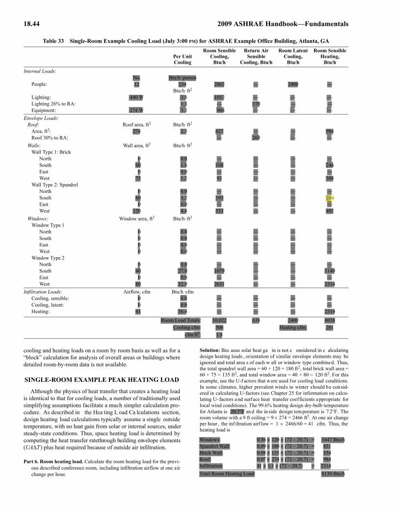
18.44 2009 ASHRAE Handbook—Fundamentals

cooling and heating loads on a room by room basis as well as for a“block” calculation for analysis of overall areas or buildings wheredetailed room-by-room data is not available.

SINGLE-ROOM EXAMPLE PEAK HEATING LOAD

Although the physics of heat transfer that creates a heating loadis identical to that for cooling loads, a number of traditionally usedsimplifying assumptions facilitate a much simpler calculation pro-cedure. As described in the Hea ting L oad Ca lculations section,design heating load calculations typically assume a single outsidetemperature, with no heat gain from solar or internal sources, understeady-state conditions. Thus, space heating load is determined bycomputing the heat transfer rate through building envelope elements(UAΔT) plus heat required because of outside air infiltration.

Part 6. Room heating load. Calculate the room heating load for the previ-ous described conference room, including infiltration airflow at one airchange per hour.

Solution: Bec ause solar heat ga in is not c onsidered in c alculatingdesign heating loads , orientation of similar envelope elements may beignored and total area s of each w all or window type combined. Thus,the total spandrel wall area = 60 + 120 = 180 ft2, total brick wall area =60 + 75 = 135 ft2, and total window area = 40 + 80 = 120 ft2. For thisexample, use the U-f actors that were used for cooling load conditions.In some climates, higher prevalent winds in winter should be consid-ered in calculating U-factors (see Chapter 25 for information on calcu-lating U- factors a nd surf ace heat transfer coef ficients a ppropriate forlocal wind conditions). The 99.6% heating design dry-bulb temperaturefor Atlanta is 20.7°F an d the in side design tem perature is 7 2°F. Theroom volume with a 9 ft ceiling = 9 × 274 = 2466 ft3. At one air changeper hour , the inf iltration airf low = 1 × 2466/60 = 41 cfm. Thus, theheating load is

Table 33 Single-Room Example Cooling Load (July 3:00 PM) for ASHRAE Example Office Building, Atlanta, GA

Per Unit Cooling

Room Sensible Cooling,

Btu/h

Return Air Sensible

Cooling, Btu/h

Room Latent Cooling,

Btu/h

Room Sensible Heating,

Btu/h

Internal Loads:No. Btu/h·person

People: 12 234 2802 — 2400 —Btu/h·ft2

Lighting: 440 W 3.8 1052 — — —Lighting 26% to RA: 1.3 — 370 — —Equipment: 274 W 3.3 904 — — —

Envelope Loads:Roof: Roof area, ft2 Btu/h·ft2

Area, ft2: 274 2.3 627 — — 984Roof 30% to RA: — 269 — —

Walls: Wall area, ft2 Btu/h·ft2Wall Type 1: Brick

North 0 0.0 — — — —South 60 1.8 108 — — 246East 0 0.0 — — — —West 75 1.2 93 — — 308

Wall Type 2: SpandrelNorth 0 0.0 — — — —South 60 3.2 193 — — 246East 0 0.0 — — — —West 120 4.4 533 — — 492

Windows: Window area, ft2 Btu/h·ft2Window Type 1

North 0 0.0 — — — —South 0 0.0 — — — —East 0 0.0 — — — —West 0 0.0 — — — —

Window Type 2North 0 0.0 — — — —South 40 27.0 1079 — — 1149East 0 0.0 — — — —West 80 32.9 2631 — — 2314

Infiltration Loads: Airflow, cfm Btu/h·cfmCooling, sensible: 0 0.0 — — — —Cooling, latent: 0 0.0 — — — —Heating: 41 56.4 — — — 2314

Room Load Totals: 10,022 638 2400 8038Cooling cfm: 506 Heating cfm: 261

cfm/ft2: 1.8

Windows: 0.56 × 120 × (72 – 20.7) = 3447 Btu/hSpandrel Wall: 0.09 × 180 × (72 – 20.7) = 831Brick Wall: 0.08 × 135 × (72 – 20.7) = 554Roof: 0.07 × 274 × (72 – 20.7) = 984Infiltration: 41 × 1.1 × (72 – 20.7) = 2314Total Room Heating Load: 8130 Btu/h

Nonresidential Cooling and Heating Load Calculations 18.45

WHOLE-BUILDING EXAMPLEBecause a single-room example does not illustrate the full appli-

cation o f lo ad calculations, a multistory, m ultiple-room e xamplebuilding has been developed to show a more realistic case. A hypo-thetical p roject development pro cess i s described to illustrate itseffect on the application of load calculations.

Design Process and Shell Building DefinitionA de velopment compan y has acquired a piece of pro perty in

Atlanta, GA, to construct an office building. Although no tenant orend user has yet been identified, the owner/developer has decided toproceed with the project on a speculative basis. They select an archi-tectural de sign firm, who retain s an engineering f irm for th emechanical and electrical design.

At the first meeting, the developer indicates the project is to pro-ceed on a fast-track basis to take advantage of market conditions;he is negotiating with several potential tenants who will need tooccupy the new b uilding wi thin a year. T his requi res pre paring

shell-and-core construction documents to obtain a b uilding per-mit, order equipment, and begin construction to meet the schedule.

The sh ell-and-core design documents will include f inisheddesign of the building exterior (the shell), as well as permanent inte-rior elements such as stai rs, restrooms, elevator, e lectrical roomsand mechanical spaces (the core). The primary mechanical equip-ment must be sized and installed as part of the shell-and-core pack-age in order for the project to meet the schedule, even though thebuilding occupant is not yet known.

The architect selects a two-story design with an exterior skin oftinted, double-glazed vision glass; opaque, insulated spandrel glass,and brick pilasters. The roof area extends beyond the building edgeto form a substantial overhang, shading the second floor windows.Architectural drawings for the shell-and-core package (see Figures17 to 22) include p lans, elevations, and skin con struction details,and are furnished to the engineer for us e in “block” hea ting andcooling load calculations. Mechanical systems and equipment mustbe specified and installed based on those calculations. (Note: Full-size, scalable electronic versions of the drawings in Figures 17 to

Table 34 Single-Room Example Peak Cooling Load (September 5:00 PM) for ASHRAE Example Office Building, Atlanta, GA

Per Unit Cooling

Room Sensible Cooling,

Btu/h

Return Air Sensible

Cooling, Btu/h

Room Latent Cooling,

Btu/h

Room Sensible Heating,

Btu/h

Internal Loads:No. Btu/h·person

People: 12 234 2802 — 2400 —Btu/h·ft2

Lighting: 440 W 3.8 1052 — — —Lighting 20% to RA: 1.3 — 370 — —Equipment: 274 W 3.3 904 — — —

Envelope Loads:Roof: Roof area, ft2 Btu/h·ft2

Area, ft2: 274 2.1 573 — — 984Roof 30% to RA: — 246 — —

Walls: Wall area, ft2 Btu/h·ft2Wall Type 1: Brick

North 0 0.0 — — — —South 60 1.9 116 — — 246East 0 0.0 — — — —West 75 1.2 90 — — 308

Wall Type 2: SpandrelNorth 0 0.0 — — — —South 60 3.7 220 — — 246East 0 0.0 — — — —West 120 4.8 570 — — 492

Windows: Window area, ft2 Btu/h·ft2Window Type 1

North 0 0.0 — — — —South 0 0.0 — — — —East 0 0.0 — — — —West 0 0.0 — — — —

Window Type 2North 0 0.0 — — — —South 40 27.1 1084 — — 1149East 0 0.0 — — — —West 80 33.9 2715 — — 2298

Infiltration Loads: Airflow, cfm Btu/h·cfmCooling, sensible: 0 0.0 — — — —Cooling, latent: 0 0.0 — — — —Heating: 41 56.4 — — — 2314

Room Load Totals: 10,126 615 2400 8038Cooling cfm: 511 Heating cfm: 261

cfm/ft2: 1.9

18.46 2009 ASHRAE Handbook—Fundamentals

22, as well as detailed lighting plans, are available from ASHRAEat www.ashrae.org.)

The HVAC design en gineer meets with the de veloper’s opera-tions staff to agree on the basic HVAC systems for the project. Basedon their experience operating other buildings and the lack of specificinformation on the tenant(s), the team decid es on two variable-volume air-handling units (AHUs), one per floor, to provide operat-ing flexibility if one floor is leased to one tenant and the other floorto someone else. Cooling will be provided by an air-cooled chillerlocated on grade across the parking lot. Heating will be provided byelectric resistance heaters in parallel-type fan-powered variable-air-volume (VAV) terminal units. The AHUs must be sized quickly toconfirm the size of the mechanical rooms on the architectural plans.The AHUs and chiller must be ordered by the mechanical subcon-tractor within 10 days to meet the construction schedule. Likewise,the electric heating loads must be provided to the electrical engi-neers to size the electrical service and for the utility company toextend services to the site.

The mechanical engineer must determine the (1) peak airflowand cooling coil capacity for each AHU, (2) peak cooling capacityrequired for the chiller, and (3) total heating capacity for sizing theelectrical service.

Solution: First, calculate “block” heating and cooling loads foreach floor to size th e AHUs , then calculate a block load for thewhole building determine chiller and electric heating capacity.

Based on the architectural drawings, the HVAC engineer assem-bles basic data on the building as follows:

Location: Atlanta, GA. Per Ch apter 14, latitude = 33.64, longi-tude = 84.43, ele vation = 1027 ft above sea le vel, 99.6% heatingdesign dry-bulb temperature = 20.7°F. F or coolin g load calcula-tions, use 5% dry -bulb/coincident wet-b ulb monthly design dayprofile from Chapter 14 (on CD-ROM). See Table 26 for tempera-ture profiles used in these examples.

Inside design conditions: 72°F for heating; 75°F with 50% rh forcooling.

Building orientation: Plan north is 30° west of true north.Gross area per floor: 15,050 ft2Total building gross area: 30,100 ft2Windows: Bronze-tinted, double-glazed. Solar heat gain coeffi-

cients, U-factors are as in the single-room example.Walls: Part insulated spandrel g lass and par t bri ck-and-block

clad columns. The i nsulation barrier in the sof fit at the secondfloor is similar to that of the sp andrel glass and is of lightweightconstruction; for simplicity, that surface is assumed to have simi-lar thermal heat gain/loss to the spandrel glass. Construction andinsulation values are as in single-room example.

Roof: Metal deck, topped with boa rd insulation and membraneroofing. Construction and insulati on v alues are as i n t he si ngle-room example.

Floor: 5 in. lightweight concrete slab on grade for first floor and5 in. lightweight concrete on metal deck for second floor

Total areas of building exterior skin, as measured from the archi-tectural plans, are listed in Table 35.

The engineer needs additional data to estimate the building loads.Thus far, no tenant has yet been signed, so no interior layouts forpopulation counts, lighting layouts or equipment loads are available.

To meet the schedule, assumptions must be made on these load com-ponents. The owner requires that the system design must be flexibleenough to provide for a variety of tenants over the life of the building.Based on similar office buildings, the team agrees to base the blockload calculations on the following assumptions:

Occupancy: 7 people per 1000 ft2 = 143 ft2/personLighting: 1.5 W/ft2Tenant’s office equipment: 1 W/ft2

Normal use schedule is assumed at 100% from 7:00 AM to7:00 PM and unoccupied/off during other hours.

With interior finishes not finalized, the owner commits to usinglight-colored in terior blinds on all windo ws. The tenant interiordesign could include carpeted flooring or acoustical tile ceilings inall areas, but the more conservative assumption, from a peak loadstandpoint, is chosen: carpeted flooring and no acoustical tile ceil-ings (no ceiling return plenum).

For block loads, the engineer a ssumes that the building is main-tained under positive pressure during peak cooling conditions and thatinfiltration during peak heati ng conditions is equi valent to one airchange per hour in a 12 ft deep perimeter zone around the building.

To maintain indoor air quality , outside air must be introducedinto the building. Air will be ducted from roof intake hoods to theAHUs where it will be mix ed with return air before being cooledand dehumidified by the AHU’ s cooling coil. ASHRAE Standard62.1 is the d esign basis for ventilation rates; ho wever, no interiortenant layout is available for application of Standard 62.1 p roce-dures. Based on past experience, the engineer decides to use 20cfmof outside air per person for sizing the cooling coils and chiller.

Block load calculations were performed using the RTS method,and results for the first and second floors and the entire building aresummarized in Tables 36, 37, and 38. Based on these results, theengineer performs psyc hrometric coi l ana lysis, checks ca pacitiesversus vendor catalog data, and prepares specifications and sched-ules for the equipment. This information is released to the contrac-tor wit h the she ll-and-core design documents. The air -handlingunits and chiller are purchased, and construction proceeds.

Tenant Fit Design Process and DefinitionAbout halfway through construction, a tenant agrees to lease the

entire building. The tenant will require a combination of open andenclosed office space with a few common areas, such as conference/training rooms, and a small compu ter room that will operate on a24 h basis. Based on the tenant’s space program, the architect pre-pares interior floor plans and furniture layout plans (Figures 23 and24), a nd t he electrical engineer prepares lighting design plans.Those dra wings are furnished to th e HVAC engineer to preparedetailed design documents. The first step in this process is to pre -pare room-by-room peak heating and cooling load calculations,which will then be use d for design of the air distribution systemsfrom each of the VAV air handlers already installed.

The HVAC engineer must perform a room-by-room “takeoff” ofthe a rchitect’s drawings. For each room, this effort identifies thefloor ar ea, roo m function, exterior envelope elements and are as,number of occupants, and lighting and equipment loads.

The t enant l ayout calls for a dropped acoustical t ile ceilingthroughout, which will be used as a return ai r plenum. Typical 2 by4 ft fluorescent, recessed, return-air -type lighting f ixtures are

Table 35 Block Load Example: Envelope Area Summary, ft2

Floor Area

Brick Areas Spandrel/Soffit Areas Window AreasNorth South East West North South East West North South East West

First Floor 15,050 680 680 400 400 700 700 360 360 600 560 360 360Second Floor 15,050 510 510 300 300 1040 1000 540 540 560 600 360 360

Building Total 30,100 1190 1190 700 700 1740 1700 900 900 1160 1160 720 720

Nonresidential Cooling and Heating Load Calculations 18.47

selected. Based on t his, the engineer assumes that 20% of the heatgain from lighting will be to the return air plenum and not enter roomsdirectly. Likewise, some portion of the heat gain from the roof will beextracted via the ceiling return air plenum. From experience, the engi-neer understands that return air plenum paths are not always predict-able, and decides to credit only 30% of the roof heat gain to the returnair, with the balance included in the room cooling load.

For the open office areas, some areas along the building perime-ter wi ll have di fferent load ch aracteristics f rom p urely in teriorspaces because of heat gains and losses through the b uilding skin.

Although those perimeter areas are not separated from other openoffice spaces by w alls, the engi neer knows from experience thatthey must be served by separate control zones to maintain comfortconditions. The data compiled from the room-by-room takeoff areincluded in Tables 39 and 40.

Room by Room Cooling and Heating LoadsThe room by room results of RTS method calculations, includ-

ing the month and time of day of each room’s peak cooling load,are t abulated in suppl emental T ables 41 and 42 (a vailable at

Table 36 Block Load Example—First Floor Loads for ASHRAE Example Office Building, Atlanta, GA

Room Loads:aPer Unit Cooling

Room Sensible Cooling,

Btu/h

Return Air Sensible

Cooling, Btu/h

Room Latent Cooling,

Btu/h

Room Sensible Heating,

Btu/h

Internal Loads:No. Btu/h·person

People: 105 238 24,675 — 21,000 —Btu/h·ft2

Lighting: 22,575 W 4.9 73,284 — — —Lighting 0% to RA: 0.0 — — — —Equipment: 15,050 W 3.3 49,780 — — —

Envelope Loads:Roof: Roof area, ft2 Btu/h· ft2 —

Area, ft2: — 0.0 — — — —Roof 0% to RA: — — — —

Walls: Wall area, ft2 Btu/h· ft2Wall Type 1: Brick

North 680 1.3 894 — — 2791South 680 1.9 1297 — — 2791East 400 1.9 743 — — 1642West 400 1.6 639 — — 1642

Wall Type 2: Spandrel North 700 3.2 2264 — — 2873South 700 2.8 1966 — — 2873East 360 2.6 943 — — 1477West 360 5.2 1872 — — 1477

Windows: Window area, ft2 Btu/h· ft2Window Type 1:

North 600 36.5 21,924 — — 17,237South 560 24.4 13,665 — — 16,088East 360 24.3 8755 — — 10,342West 360 64.0 23,040 — — 10,342

Window Type 2: North 0 0.0 — — — —South 0 0.0 — — — —East 0 0.0 — — — —West 0 0.0 — — — —

Infiltration Loads: Airflow, cfm Btu/h·cfmCooling, sensible: 0 0.0 — — — —Cooling, latent: 0 0.0 — — — —Heating: 863 56.4 — — — 48,499

Room Load Totals: 225,741 — 21,000 120,273Cooling cfm: 11,401 Heating cfm: 3905

cfm/ft2: 0.8

Block Loads:b Total Room Sensible + RA + Latent: 246,741 Room heating: 120,273Outside air (OA) sensible: 36,498 OA heating: 118,503

OA cfm: 2100 OA latent: 50,267 Total heating, Btu/h: 238,776Fan hp: 10 Fan heat to supply air: 25,461 Heating Btu/h·ft2: 15.9

Pump hp: 0 Pump heat to chilled water: —tons ft2/ton

Total Block Cooling Load, Btu/h: 358,967 29.9 503aPeak room sensible load occurs in month 7 at hour 16.bPeak block load occurs in month 7 at hour 16.

18.48 2009 ASHRAE Handbook—Fundamentals

www.ashrae.org), as well as peak heati ng loads for each room.These results are used by the HVAC engineer to select and designroom air distribution devices and to schedule airflow rates for eachspace. That information is incorpor ated into the tenant f it draw-ings and specifications issued to the contractor.

ConclusionsThe example results illustrate issues which should be understood

and accounted for in calculating heating and cooling loads:

• First, peak room cooling loads occur at dif ferent months andtimes depending on the exterior exposure of the room. Calcula-tion of cooling loads for a single point in time may miss the peakand result in inadequate cooling for that room.

• Often, in real design processes, all data is not known. Reasonableassumptions based on past experience must be made.

• Heating and air-conditioning systems often serve spaces whose usechanges over the l ife of a b uilding. Assumptions used in heatingand cooling load calculations should consider reasonable possibleuses over the life of the building, not just the first use of the space.

Table 37 Block Load Example—Second Floor Loads for ASHRAE Example Office Building, Atlanta, GA

Room Loads:aPer Unit Cooling

Room Sensible Cooling,

Btu/h

Return Air Sensible

Cooling, Btu/h

Room Latent Cooling,

Btu/h

Room Sensible Heating,

Btu/h

Internal Loads:No. Btu/h·person

People: 105 234 24,518 — 21,000 —Btu/h·ft2

Lighting: 22,575 W 4.8 72,915 — — —Lighting 0% to RA: 0.0 — — —Equipment: 15,050 W 3.4 49,626 — — —

Envelope Loads:Roof: Roof area, ft2 Btu/h· ft2

Area, ft2: 15,050 3.3 49,202 — — 54,045Roof 0% to RA: — — — —

Walls: Wall area, ft2 Btu/h· ft2Wall Type 1: Brick

North 510 1.1 565 — — 2093South 510 1.8 915 — — 2093East 300 1.8 545 — — 1231West 300 1.2 373 — — 1231

Wall Type 2: Spandrel North 1040 2.8 2865 — — 4268South 1000 3.2 3224 — — 4104East 540 2.8 1491 — — 2216West 540 4.4 2398 — — 2216

Windows: Window area, ft2 Btu/h· ft2Window Type 1:

North 0 0 — — — —South 0 0 — — — —East 0 0 — — — —West 0 0 — — — —

Window Type 2: North 560 28.4 15,916 — — 16,088South 600 27.0 16,188 — — 17,237East 360 26.1 9,389 — — 10,342West 360 32.9 11,840 — — 10,342

Infiltration Loads: Airflow, cfm Btu/h·cfmCooling, sensible: 0 0.0 — — — —Cooling, latent: 0 0.0 — — — —Heating: 863 56.4 — — — 48,699

Room Load Totals: 261,968 — 21,000 176,205Cooling cfm: 13,231 Heating cfm: 5721

cfm/ft2: 0.9Block Loads:b Total Room Sensible + RA + Latent: 282,968 Room heating: 176,205

Outside air (OA) sensible: 39,270 OA heating: 118,503OA cfm: 2100 OA latent: 50,908 Total heating, Btu/h: 294,708Fan hp: 10 Fan heat to supply air: 25,461 Heating Btu/h·ft2: 19.6

Pump hp: 0 Pump heat to chilled water: —tons ft2/ton

Total Block Cooling Load, Btu/h: 398,607 33.2 453aPeak room sensible load occurs in month 7 at hour 15.bPeak block load occurs in month 7 at hour 15.

Nonresidential Cooling and Heating Load Calculations 18.49

• The relative importance of each cooling and heating load compo-nent varies depending on the por tion of the b uilding being con-sidered. Characteristics of a pa rticular window may have littleeffect on the entire building load , but could have a signif icanteffect on the supply airflow to the room where the window islocated and thus on the comfort of the occupants of that space.

PREVIOUS COOLING LOAD CALCULATION METHODS

Procedures described in this chapter are the most current and sci-entifically derived means for estimating cooling load for a definedbuilding space, b ut methods in earlier editions of the ASHRAEHandbook are valid for many applications. These earlier proceduresare simplifications of the heat balance principles , and their userequires experience to deal with atypical or unusual circumstances.In fact, any cooling or heating load estimate is no better than theassumptions used to define conditions and parameters such as phys-ical makeup of the various envelope surfaces, conditions of occu-pancy and use, and ambient weathe r conditions. Experience of thepractitioner can never be ignored.

The primary difference between the HB and RTS methods andthe older methods is the newer methods’ direct approach, comparedto the simplifications necessitated by the limited computer capabil-ity available previously.

The transfer function method (TFM) , for example, requiredmany calculation steps. It was originally designed for energy anal-ysis with emphasis on daily, monthly, and annual energy use, andthus was more oriented to average hourly cooling loads than peakdesign loads.

The total equi valent tem perature differ ential m ethod withtime averaging (TETD/TA) has been a highly reliable (if subjec-tive) method of load estimating since its initial presentation in the1967 Handbook of Fundamentals. Originally intended as a manualmethod of calculation, it proved suitable only as a computer appli-cation because of the need to calculate an extended profile of hourlyheat gain values, from which radiant components had to be averagedover a time representati ve of the gener al mass of the building in-volved. Because perception of thermal storage characteristics of agiven building is almost entirely subjective, with little specific in-formation for the user to judge variations, the TETD/TA method’sprimary usefulness has always been to the experienced engineer.

The cooling load temperature differential method with solarcooling load factors (CLTD/CLF) attempted to simplify the two-step TFM and TETD/TA methods into a single-step technique thatproceeded directly f rom raw data to cooling load without inter -mediate conversion of radiant heat gain to cooling load. A series offactors were taken from cooling load calculation results (produced

by more sophisticated methods) as “cooling load temperature dif-ferences” and “cooling load factors” for use in traditional conduc-tion (q = UAΔt) equations. The results are approximate cooling loadvalues rather than simple heat gain values. The simplifications andassumptions used in the original work to derive those factors limitthis method’s applicability to those building types and conditionsfor which the CLTD/CLF factors were derived; the method shouldnot be used beyond the range of applicability.

Although the TFM, TETD/TA, and CLTD/CLF procedures arenot republished in this chapter, those methods are not invalidated ordiscredited. Experienced engineers have successfully used them inmillions o f buildings around the world. The accuracy o f coolingload calculations in practice depends primarily on the availability ofaccurate infor mation and the design eng ineer’s judg ment in theassumptions made in interpreting the available data. Those factorshave much greater inf luence on a pr oject’s success than d oes thechoice of a particular cooling load calculation method.

The primary benefit of HB and RTS calculations is their some-what reduced depen dency on purely subjective input (e.g., deter-mining a proper time-averaging period for TETD/TA; ascertainingappropriate safety f actors to ad d to the rounded-of f TFM results;determining whether CLTD/CLF factors are applicable to a specificunique application). However, using the most up-to-date techniquesin real-world design still requires judgment on the part of the designengineer and car e in choosing appropriate assumptions, just as inapplying older calculation methods.

REFERENCESAbushakra, B., J.S. Haberl, and D.E. Claridge. 2004. Overview of literature

on diversity factors and schedules for energy and cooling load calcula-tions (1093-RP). ASHRAE Transactions 110(1):164-176.

Armstrong, P.R., C .E. Han cock, III, and J.E . Seem. 1992a. Commer cialbuilding temperature recovery—Part I: Design procedure based on a stepresponse model. ASHRAE Transactions 98(1):381-396.

Armstrong, P.R., C.E. Han cock, I II, and J.E. Seem. 1992b. Commer cialbuilding temperature recovery—Part II: Experiments to verify the stepresponse model. ASHRAE Transactions 98(1):397-410.

ASHRAE. 2004. Thermal environmental conditions for human occupancy.ANSI/ASHRAE Standard 55-2004.

ASHRAE. 2001. V entilation for a cceptable indoor air quality . AN SI/ASHRAE Standard 62-2001.

ASHRAE. 2007. Energy standard for building except low-rise residentialbuildings. ANSI/ASHRAE/IESNA Standard 90.1-2007.

ASHRAE. 2004. Updating the clim atic design conditions in the ASHRAEHandbook—Fundamentals (RP- 1273). ASH RAE Resear ch Pr oject,Final Report.

ASTM. 2008. Practice for estimate of the heat gain or loss and the surfacetemperatures of insulated flat, cylindrical, and spherical systems by useof computer programs. Standard C680-08. American Society for Testingand Materials, West Conshohocken, PA.

Table 38 Block Load Example—Overall Building Loads for ASHRAE Example Office Building, Atlanta, GARoom Sensible

Cooling,Btu/h

Return Air Sensible

Cooling, Btu/h

Room Latent Cooling,

Btu/h

Room Sensible Heating,

Btu/h

Room Loadsa Room Load Totals: 483,550 — 42,000 296,478Cooling cfm: 24,422 Heating cfm: 9626

cfm/ft2: 0.8Block Loads:b Total Room Sensible + RA + Latent: 525,550 Room heating: 296,478

Outside air (OA) sensible: 91,540 OA heating: 237,006OA cfm: 4200 OA latent: 101,816 Total heating, Btu/h: 533,484Fan hp: 20 Fan heat to supply air: 50,922 Heating Btu/h·ft2: 17.7

Pump hp: 5 Pump heat to chilled water: 12,730tons ft2/ton

Total Block Cooling Load, Btu/h: 782,558 65.2 462aPeak room sensible load occurs in month 7 at hour 15.bPeak block load occurs in month 7 at hour 15.

18.52 2009 ASHRAE Handbook—Fundamentals

Bliss, R.J.V. 1961. Atmospheric radiation near the surface of the ground.Solar Energy 5(3):103.

Chantrasrisalai, C., D.E. Fisher, I. Iu, and D. Eldridge. 2003. Experimentalvalidation of design cooling load procedures: The heat balance method.ASHRAE Transactions 109(2):160-173.

Claridge, D.E ., B. Ab ushakra, J.S. Haberl, an d A. Sr eshthaputra. 20 04.Electricity diversity prof iles for energy simulation of of fice buildings(RP-1093). ASHRAE Transactions 110(1):365-377.

Eldridge, D., D.E. Fisher, I. Iu, and C. Chantrasrisalai. 2003. Experimentalvalidation of design cooling load procedures: Facility design (RP-1117).ASHRAE Transactions 109(2):151-159.

Fisher, D.R. 1998. New recommended heat gains for commercial cookingequipment. ASHRAE Transactions 104(2):953-960.

Fisher, D.E. and C. Chantrasrisalai. 2006. Lighting heat gain distribution inbuildings (RP-1282). ASHRAE Research Project, Final Report.

Fisher, D.E. and C.O. Pedersen. 1997. Convective heat transfer in buildingenergy and thermal load calculations . ASHRAE Transactions 10 3(2):137-148.

Gordon, E.B., D.J. Horton, and F.A. Parvin. 1994. Development and appli-cation of a s tandard test method for the per formance of exhaust hoodswith commercial cooking appliances. ASHRAE Transactions 100(2).

Hittle, D.C. 1999. The effect of beam solar radiation on peak cooling loads.ASHRAE Transactions 105(2):510-513.

Hittle, D.C. a nd C.O. Pedersen. 1981. Calculating b uilding heating loadsusing th e f requency of mu lti-layered slabs. ASHRAE T ransactions87(2):545-568.

Hosni, M.H. and B.T. Beck. 2008. Update to measurements of office equip-ment heat gain data (RP-1482). ASHRAE Research Project, ProgressReport.

Hosni, M.H., B.W. Jones, J.M. Sipes, and Y. Xu. 1998. Total heat gain andthe split between radiant and convective heat gain from office and labo-ratory equipment in buildings. ASHRAE Transactions 104(1A):356-365.

Hosni, M.H., B.W. Jones, and H. Xu. 1999. Experimental results for heatgain and radiant/convective split from equipment in buildings. ASHRAETransactions 105(2):527-539.

Incropera, F.P. and D.P DeWitt. 1990. Fundamentals of heat and mass trans-fer, 3rd ed. Wiley, New York.

Iu, I. and D.E. Fisher. 2004. Application of conduction transfer functionsand p eriodic r esponse f actors in cooling loa d calculation procedures.ASHRAE Transactions 110(2):829-841.

Iu, I., C. Chantrasrisalai, D.S. Eldridge, and D.E. Fisher. 2003. experimentalvalidation of design cooling load procedures: T he radiant time seriesmethod (RP-1117). ASHRAE Transactions 109(2):139-150.

Jones, B.W., M.H. Hosni, and J.M. Sipes. 1998. Measurement of radiantheat gain from office equipment using a scanning radiometer. ASHRAETransactions 104(1B):1775-1783.

Karambakkam, B.K., B. Nigusse, and J.D. Spitler. 2005. A one-dimensionalapproximation for transient multi-dimensional conduction heat transferin building envelopes. Proceedings of the 7th Symposium on BuildingPhysics in the Nordic Countries, The Icelandic Building Research Insti-tute, Reykjavik, vol. 1, pp. 340-347.

Kerrisk, J.F., N.M. Schnurr, J.E. Moore, and B.D. Hunn. 1981. The customweighting-factor method for ther mal loa d calculations in the DOE -2computer program. ASHRAE Transactions 87(2):569-584.

Komor, P. 1997. Space cooling demands from office plug loads. ASHRAEJournal 39(12):41-44.

Kusuda, T. 1967. NBSLD, the computer program for heating and coolingloads for b uildings. BSS 69 and NBSIR 74- 574. National Bureau ofStandards.

Latta, J.K. and G. G. Boileau. 1969. Heat los ses fr om hou se basements.Canadian Building 19(10):39.

LBL. 2003. WINDOW 5.2: A P C program for an alyzing window thermalperformance for fenestration products. LBL-44789. Windows and Day-lighting Group. Lawrence Berkeley Laboratory, Berkeley.

Liesen, R.J. and C.O. Pedersen. 1997. An evaluation of inside surface heatbalance models for cooling load calc ulations. ASHRAE T ransactions103(2):485-502.

Marn, W.L. 1962. Commercial ga s kitchen ventilation studies. ResearchBulletin 90(March). Gas Association Laboratories, Cleveland, OH.

McClellan, T.M. and C.O. Pedersen. 1997. Investigation of outside heat bal-ance models for use in a heat balance cooling load calculation procedure.ASHRAE Transactions 103(2):469-484.

McQuiston, F.C. and J.D. Spitler. 1992. Cooling and heating load calcula-tion manual, 2nd ed. ASHRAE.

Miller, A. 1971. Meteorology, 2nd ed. Charles E. Merrill, Columbus.Nigusse, B.A. 2007. Improvements to the radiant time series method cooling

load calculation procedure. Ph.D. dissertation, Oklahoma State Univer-sity.

Parker, D.S., J.E.R. McIlvaine, S.F. Barkaszi, D. J. Beal, and M. T. Anello.2000. Laboratory testing of the reflectance properties of roofing mate-rial. FSEC-CR670-00. Florida Solar Energy Center, Cocoa.

Pedersen, C.O., D.E. Fisher, and R.J. Liesen. 1997. Development of a heatbalance procedure for calculating cooling loads. ASHRAE Transactions103(2):459-468.

Pedersen, C.O., D.E. Fisher, J.D. Spitler, and R.J. Liesen. 1998. Cooling andheating load calculation principles. ASHRAE.

Rees, S.J., J.D. Spitler, M.G. Davies, and P. Haves. 2000. Qualitative com-parison of North American and U.K. cooling load calculation methods.International Journal of Heating , Ventilating, A ir-Conditioning andRefrigerating Research 6(1):75-99.

Rock, B.A. 2005. A user-friendly model and coefficients for slab-on-gradeload and energy calculation. ASHRAE Transactions 111(2):122-136.

Rock, B.A. and D.J. Wolfe. 1997. A sensitivity study of floor and ceiling ple-num energy model parameters. ASHRAE Transactions 103(1):16-30.

Smith, V .A., R.T . Swier czyna, and C. N. Claar . 1 995. Application andenhancement of the standa rd test method for the pe rformance of com-mercial kitchen ventilation systems. ASHRAE Transactions 101(2).

Sowell, E.F. 1988a. Cross-check and modification of the DOE-2 programfor calculation of zone weighting factors. ASHRAE Transactions 94(2).

Sowell, E.F. 1988b. Load calculations for 200,640 zones. ASHRAE Trans-actions 94(2):716-736.

Spitler, J.D. and D.E. Fisher. 1999a. Development of periodic response fac-tors for use with the radiant time series method. ASHRAE Transactions105(2):491-509.

Spitler, J.D. and D.E. Fisher. 1999b. On the relationship between the radianttime series and transfer function methods for design cooling load calcu-lations. International Journal of Heating, Ventilating, Air-Conditioningand Refrigerating Research (now HVAC&R Research) 5(2):125-138.

Spitler, J.D., D.E. Fisher, and C.O. Pedersen. 1997. The radiant time seriescooling load calculation procedure. ASHRAE Transactions 103(2).

Spitler, J.D., S.J. Rees, and P. Haves. 1998. Quantitive comparison of NorthAmerican and U.K. cooling load calculation procedures—Part 1: Meth-odology, Part II: Results. ASHRAE Transactions 104(2):36-46, 47-61.

Sun, T.-Y. 1968. Shadow area equations for window overhangs and side-finsand their application in computer calc ulation. ASHRAE Transactions74(1):I-1.1 to I-1.9.

Swierczyna, R., P. Sobiski, and D. Fisher. 2008. Revised heat gain and cap-ture and con tainment e xhaust r ates from typical commercia l cookingappliances (RP-1362). ASHRAE Research Project, Final Report.

Swierczyna, R., P.A. Sobiski, and D.R. Fisher. 2009 (forthcoming). Revisedheat gain rates from typical commercial cooking appliances from RP-1362. ASHRAE Transactions 115(2).

Talbert, S.G., L.J. Canigan, and J.A. Eibling. 1973. An experimental studyof ventilation requirements of commercial electr ic kitchens. ASHRAETransactions 79(1):34.

Walton, G. 1 983. Thermal a nalysis research program reference man ual.National Bureau of Standards.

Wilkins, C.K. and M.R. Cook. 1999. Cooling loads in laboratories. ASHRAETransactions 105(1):744-749.

Wilkins, C.K . and M. H. Hosni. 2000. Heat gain from office equipment.ASHRAE Journal 42(6):33-44.

Wilkins, C. K. an d N. M cGaffin. 199 4. Measu ring comp uter eq uipmentloads in office buildings. ASHRAE Journal 36(8):21-24.

Wilkins, C.K., R. Kosonen, and T. Laine. 1991. An analysis of office equip-ment load factors. ASHRAE Journal 33(9):38-44.