PREFACE - Netaji Subhas Open University · Unit 4 Assignment Problem 60-79 Module 2 ... Unit 7 Inventory Management 142-195 Post-Graduate : Commerce M. Com-8 NETAJI SUBHAS OPEN UNIVERSITY.

1

PREFACE

In the curricular structure introduced by this University for students of Post-Graduate degree programme, the opportunity to pursue Post-Graduate course in anySubject introduced by this University is equally available to all learners. Instead ofbeing guided by any presumption about ability level, it would perhaps stand to reasonif receptivity of a learner is judged in the course of the learning process. That wouldbe entirely in keeping with the objectives of open education which does not believein artificial differentiation.

Keeping this in view, study materials of the Post-Graduate level in differentsubjects are being prepared on the basis of a well laid-out syllabus. The coursestructure combines the best elements in the approved syllabi of Central and StateUniversities in respective subjects. It has been so designed as to be upgradable withthe addition of new information as well as results of fresh thinking and analysis.

The accepted methodology of distance education has been followed in thepreparation of these study materials. Cooperation in every form of experienced scholarsis indispensable for a work of this kind. We, therefore, owe an enormous debt ofgratitude to everyone whose tireless efforts went into the writing, editing and devisingof a proper lay-out of the materials. Practically speaking, their role amounts to aninvolvement in ‘invisible teaching’. For, whoever makes use of these study materialswould virtually derive the benefit of learning under their collective care without eachbeing seen by the other.

The more a learner would seriously pursue these study materials, the easier itwill be for him or her to reach out to larger horizons of a subject. Care has also beentaken to make the language lucid and presentation attractive so that they may be ratedas quality self-learning materials. If anything remains still obscure or difficult tofollow, arrangements are there to come to terms with them through the counsellingsessions regularly available at the network of study centres set up by the University.

Needless to add, a great deal of these efforts is still experimental—in fact,pioneering in certain areas. Naturally, there is every possibility of some lapse ordeficiency here and there. However, these do admit of rectification and furtherimprovement in due course. On the whole, therefore, these study materials are expectedto evoke wider appreciation the more they receive serious attention of all concerned.

Professor (Dr.) Manimala DasVice-Chancellor

2

Printed in accordance with the regulations and financial assistance of theDistance Education Council, Government of India.

Fourth Reprint : July, 2011

3

Notification

All rights reserved. No part of this book may be reproduced in any form withoutpermission in writing from Netaji Subhas Open University.

Professor (Dr.) Bikas GhoshRegistrar (Acting)

POST-GRADUATE : COMMERCE[M. COM.]

Paper – 8Modules 1 & 2

Quantitative Techniques

: Course Writing : : Editing :Prof. Arup Kumar Chattopadhyay Prof. Ranajit Chakrabarty

5

Module1

Unit 1 p Introduction to Operation Research 1-10

Unit 2 p Linear Programming 11-38

Unit 3 p Transportation Problem 39-59

Unit 4 p Assignment Problem 60-79

Module2

Unit 5 p Theory of Games 80-106

Unit 6 p Project Management PERT and CPM 107-141

Unit 7 p Inventory Management 142-195

Post-Graduate : CommerceM. Com-8

NETAJI SUBHASOPEN UNIVERSITY

1

Unit 1 p Introduction to Operations Research

Structure

1.0 Objectives

1.1 Introduction

1.2 Historical Development

1.3 Operations Research approach

1.3.1 Definition of Operations Research

1.4 Phases of Operations Research Study

1.4.1 Problem Defining Phase

1.4.2 Model Construction Phase

1.4.3 Model solution Phase

1.4.4 Model Validity Phase

1.4.5 Implementation Phase

1.5 Tools and Techniques of O.R. Study

1.5.1 Allocation Techniques

1.5.2 Inventory Determining Techniques

1.5.3 Decision Analysis Techniques

1.5.4 Network Analysis Techniques

1.5.5 Other O.R. Techniques

1.6 Scope of Operations Research

1.7 Summary

1.8 Exercises

1.9 References

2

1.0 Objectives

The Objectives of this unit are to :

l describe the historical development of the study of Operations Research

l highlight the basic features of Operations Research

l illustrate the methods and tools broadly used in Operations Researchstudy

l discuss the scope of the subject.

All these will facilitate to know the nature of the subject.

1.1 Introduction

Operations Research as a separate discipline has been developed since 1950sto solve many real life decision making problems. This study implies the use ofscientific, quantitative and logical methods and techniques to structure and solvedicision problems. Initially the techniques used in O.R. study were applied in adifferent context. But realising their importances, those techniques ae now beingused and taught as a separate discipline to solve the decision problems, speciallyin the fields like, business, commerce, management, etc.

Unlike mathematical and statistical approaches, operations research approachto solve any decision or control problems has some special features which areto be known clearly to know the subject better. This aspect is taken intoconsideration here for detailed discussion. The art of model building and the toolsrequired to handle models of operations Reserch are also analysed in this unit.The broad areas in which operations Research techniques can be applied arepointed out lastly.

3

1.2 Historical Development

During world war II a group of individuals and specialists from different fieldslike, matehmatics, statistics, economics, engineering, psychology, physical scienceetc. were employed first in England and then in the United States to achievesuccess in the war. Those academicians and professional with their joint researchon military operations devised some techniques and tools for appropriate use ofthe military resources by which was problmes (initially the problem related to thecoordination of radar equipment at gun sites) could be solved.

After the end of the war, those experts realised that the techniques whichwere iunitially applied to solve the war problems could also be used to solvedifferent civilian problems. Consequently, different scholars bagan to pay theirattentions to the development and applications of those techniques which werebrought together under a subject coined as Operations Research (as initially thetechniques were invented as a result of research on military operations). A keyperson in the post-war development of Operations Research was George B. Dantzigwho developed first the programming technique (known as simplex method ofLPP) in O.R.

A substantial progress was observed in the applications of O.R. techniquesduring 1950s. At present it is observed that in different areas of decision problemsranging from manufacturing sector to social service sector and from individuallevel to government) public administrative) level O.R. techniques are applied. Insearch of solving the real life problems through O.R. techniques, an O.R. clubwas formed also first in England and its quarterly journal was first published in1950. Similarly an O.R. society was established in America and its journal beganto be published since 1953. In India O.R. came into existence in 1949 with theestablishment of an O.R. unit in Hyderabad. In 1953 Prof. P. C. Mahalanobisformed an O.R. team in calcutta and then in 1957 the O.R. Society of India wasfounded.

1.3 Operations Research Approach

O.R. approach implies the art of tackling any decision problem with the help ofO. R. techniques. The O. R. approach has the basic four properties, namely

4

interdisciplinary, wholistic, methodological and objectivistic in nature.

1.3.1 Definition of Operations Research

According to Churchman et al. ‘Operations Research is the application ofscientific methods, techniques and tools to problems involving the operations ofsystem so as to provide those in control of operations with optimum solutions tothe problems’. So an O. R. study of a problem is its methodical and systematicstudy in which the given problem is to be translated first in the form of a modeland then optimum solution is worked out and implemented with taking care ofcontrol if requried.

1.4 Phases of Operations Research Study

To solve any given decision problem the O.R. study is conducted and controlledthrough the following steps :

(i) Definition of the problem

(ii) Construction of the model

(iii) Solution of the model

(iv) Validation of the model and

(v) Implementation of the solution.

Each of these phases is explained one by one below taking an example of resourceallocation problem.

1.4.1 Problem Defining Phase

The first phase of an O. R. study is to identify aecurately the decision problemthan can be solved by using O. R. techniques. When a problem is placed toO. R. team for getting its solution, the team will define the problem from angles,viz. (i) description of goal or objective, (ii) identification of alternative decisionsand (iii) recognition of requirements, restrictions and limitation related to theproblem.

5

1.4.2 Model Construction Phase

In this phase, the given decision problem is expressed quantiatively. For that,first, the decision variables (on which actually decisions are to be taken) areidentified. Then using the decision variables quantitative expressions for the objectivefunction(s) and constraints of the problems are specified. In this way the modelwhich is constructed may be either a mathematical model or a simulation modelor a heuristic model; that actually depends on the nature and complexity of theproblem to be studies.

1.4.3 Model Solution Phase

After the construction of the model, its solution is worked out. If theconstructed model is a mathematical one, its solution is obtained by applying somewell defined optimization techniques. Unlike in pure mathematics, here generallyoptimum solution is achieved through interactive process (i.e., by applying thesolution technique repeatedly until optimum solution is obtained). However, incase of simulation or heuristic model as the concept of optimality is not well-defined, in this case solution is obtained through the technique of approximateevaluations.

1.4.4 Model Validity PhaseThe fourth phase of an O.R. study is to examine the validity of the model. A

model is said tto be valid if it can reasonably predict the future event related to thegiven decision problem. Validation of the model can be checked from two aspects. Inthe constructed model decision varaibles are incorporated on the basis of estimatingtheir related parameters. Estimation of the parameters may not be accurate and inreality they may change. The strength of a model depends on how far the parametersare estimated accurately or due to change of the values of the parameters how far thesolution remains effective.

The validity of the model is also checked by comparing its performance usingsome past avaliable data. The model will be valid if, using past data of a system,the past performance of that system can be reproduced. For a nonexisting systemas past data cannot collected for comparison, the validation of the model can bechecked by using data generated from a simulated model or from trial runs of thesystem.

6

1.4.5 Implementation Phase

The tested results of the model are finally implemented in the system. For properimplementation, the results of the O.R. study are to be translated into detailed operatinginstructions so that the personnel who actually operate and administer the system caneasily understand the instructions; otherwise the study will be of no use. However,realising the ground reality the recommended results may be requred to be modifiedfor proper implementation.

1.5 Tools and Techniques of O.R. Study

Operations research as a subject falls under the categories of both Arts andScience. As operations research mainly deals with the solutions of decision-makingproblems, it should take into account the human behaviour on which ultimately anydecision depends. Specially for defining the decision problem, construction of theO.R. model and implementing the recommended results fruitfully the knowledgeson human behaviour and human psychology are very much requred. So any O. R.study has an aspect of Arts. To deal with other two phases (namely, solution andvalidation) along with these three phases of the O.R. study, the knowledges onmathematics, statistics and other physical, behavioural and social sciences would berequred. So the O. R. has also the science aspect. In Operations Research the toolsand techniques vary due to variation of the nature of the decision problems actuallythere are numerous tools and techniques in O.R. and some major of them arediscussed below.

1.5.1 Allocation Techniques

When the decision problem is related to optimum allocation of resourcesamong availahle alternative uses, the allocation techniques (alternatively known asprogramming techniques) are applied. In programming techniques any measure ofeffectiveness (expressed in the form of objective function) is optimized subject tosome constraints and that measure of effectiveness may be either revenue orprofit or cost or any other measure of performance. Programming techniquesinclude linear programming, transportation, assignment, non-linear programming,integer-programming, goal programming, dynamic programming, stochastic

7

programming technique etc. In this module some programming techniques will beanalysed.

1.5.2 Inventory Control TechniquesManufacturing and business firms generally face the problem of determining

optimum level of invantory (that includes raw materials, unfinished products, finishedproducts etc.) so that the inventory costs (i.e., cost of ordering, carrying cost andcost of shortage) which are conflicting in nature are properly managed. To dealwith this problem different deterministic and probabilistic inventory control modelshave been evolved. Some of these model with be discussed in the other moduleof the subject.

1.5.3 Decision Analysis TechniquesTo take decisions under risk and uncertainty and also in the competitive environment,

different decision analysis techniques for different states of nature are available. Inthese techniques, in general, given the possible payoffs (with their associated probabilitiesin case of risk) an optimal course of action or optimal strategy is seldcted, that minimisesprobable cost or maximises probable gain. The techniques which ae applied for decisionanalysis are game theory techniques (when two or more players compete for theachievement of conficting goals), decision tree analysis, analysis of pay-off matrix(using the rules of minimax, maximum, minimum opportunity loss, etc.), Markov-chairanalysis, etc.

1.5.4 Network Analysis TechniquesThese techniques are applied to the planaing, controlling and scheduling of large

projects effectively. PERT and CPM techniques are two widely used techniques in thiscategory and with these techniques we can determine the time-cost trade-off, projectcompletion time, optimum allocation of resources updating activity times, etc. Thisnetwork analysis and game theory will be analysed in the next module. However,network analysis techniques also include the techniques like, network minimisation (toconnect all the areas in a network of, say, cable connection), shortest-route algorithm,maximum-flow algorithm, etc.

1.5.5 Other O. R. Techniques

It is very difficult to give a comprehensive list of O.R. techniques ascontinuous researches are going on to improve the existing techniques and to

8

devise new techniques. However, apart from the above-mentioned techniques, someother well-known O. R. tools are queuing theory (in which costs of waiting aswell as casts of providing servers are minimised), simulation technique (when realsituation is either complex to represent quantitatively or non-existatnt), replacementtechnique (to determine the time of replacement of a machine) sequening technique(applied in derterminig the sequence or order of performing a number of jobs),etc.

1.6 Scope of Operations Research

Operations Research has wide applications in the fields of management, commerce,economics, public administration, engineering, etc. Some of the managerial decisionmaking problems which can be analysed by O. R. approach are arranged functionalarea-wise as follows.

(i) Marketing management

(a) Product selection, (b) Competitive actions, (c) Advertising and salespromotional planning, (d) Sales effort allocation and assignment, (e) size of stockdetermination to meet market demand etc.

(ii) Personnel management

(a) Recruitment policies, (b) Assignment of jobs, (c) Scheduling of trainingprogrammes, (d) Manpower planning, (e) Skill and wage balancing, etc.

(iii) Production management

(a) Logistics, layout, engineering design, (b) Transportation, (c) Productionscheduling and sequencding, (d) Inventory management and contro, (e) Optimumproduct-mix determination, (f) Quality control, (g) Maintenance and replacement ofmachineries, (h) Project scheduling, etc.

(iv) Finance and Accounting

(a) Capital budgeting and rationing, (b) Cash flow analysis, (c) Dividend policies,(d) Investment and protfolio management (e) Credit policies, (f) Claim and complaintprocedure, (g) Break-even analysis and so on.

9

(v) Other Areas

(a) Reliability and evaluation of alternative design, (b) Forecasting, (c)Communication of information, (d) Economic planning, (e) Solution of urban housingproblem, (f) Distribution of public services, (g) Military and police personnel deploykent,(h) Pollution control, (i) Solution of traffic congestion problem and many other areasrelated to decision making problem.

1.7 Summary

Let us sum up the discussions of introductory unit. Operations Researchoriginated from the researches on military operations during Wrold War-II. It wasrealised later on that the techniques of O.R. could also be used to solve manyreal life problems and as a subject O.R. came into existence from early 1950s.The main area of the O.R. study is to solve the decision-making problemsquantitatively. The O.R. approach required to solve any decision problem isinterdisciplinary as well as wholistic in nature. Further, the O. R. study, the decisionproblem is requried to be known accurately and categorically. Then the problemis to be represented in teh form of a model which is solved by applying O.R.techniques. Ultimately the solution is implemented, of course after checking thevalidity of the model.

There are different tools and techniques of the O.R. study and these are appliedto achieve solutions of decision problems by using either non-interactive analyticalmethod or interactive numerical method or Monte Carlo method. However, themajor techniques of O. R. are programming techniques, decision analysis techniques,inventory and network analysis techniques, simulation techniques etc. Thesetechniques can be applied to solve many real life decision making problems indifferent fields of business, management, economics, engineering publicadministraction and so on.

10

1.8 Exercise

1. What is O.R.? Briefly review its origin and development.

2. Briefly discuss the essential characteristics of Operations Research.

3. Mention different phases in an O. R. study.

4. Give applications of O.R. in industry.

5. Briefly discuss the major techniques of Operations Research.

6. Explain the role of Operations Research in Management.

7. Do you think that O.R. is a subject of Arts of Science? Give reasons for youranswer.

1.9 References

1. V. K. Kapoor : Operations Research, Sultan Chand & Sons, NewDelhi.

2. H. A. Taha : Operations Research—An Introduction, Macmillan,New York.

3. N. D. Vohra : Quantitative Techniques in management, Tata McGrawHill, New Delhi.

11

Unit 2 p Linear Programming

Structure

2.0 Objectives

2.1 Introduction

2.2 Features of LP Problems

2.3 Formulation of LP Problems

2.4 Solution of LP

2.4.1 Graphical Solution of LP Problems

2.4.2 Exceptional Cases in LP Solution

2.5 Technical Issues in linear Programming

2.5.1 Different forms of LP

2.5.2 Different Solutions of LP

2.5.3 Fundamental Theorem of LP

2.6 Simplex Method theorem of LP

2.6.1 Use of Simplex Method in Maximisation Problem

2.6.2 Use of Simplex Method in Minimisation Problem

2.6.3 Some Special cares in Simplex Method

2.7 Duality in Linear Programming

2.7.1 Dual Formulation

2.7.2 Important Theorems on Duality

2.7.3 Primal-Dual Relationship

2.8 Summary

2.9 Exercises

2.10 References

12

2.0 Objectives

The objectives of this unit are to introduce and explain the followingissues :

l Features of linear programming problems

l Formulation of linear programming problems

l Graphical Solution of linear programming problems

l Algebraic solution (i.e., simplex method) of linear programmingproblems

l Dual formulation of linear programming problmes

l Primal-dual relationships

After knowing all these issues one will be able to take decisions independentlyin cases of allocation of scarce resources, choice of multiple products, etc., all of whichcan be put in the special format of the linear programming.

2.1 Introduction

Linear Programming (LP) is an optimization technique that was introduced bythe Russian mathematician L. Kantorovich. Later on in 1947 this programmingtechnique was developed by George B. Dantzig. In real life situations and indifferent fields, this programming technique can be applied to solve the decisionmaking problem of linear type.

LP is the analysis of problems in which a linear function of a number ofdecision variables is maximised or minimised when those variables are subject toa number of constraints in the form of linear equalities or inequalities. In orderto maximise or minimise any function subject to some constraints, we can applyclassical constrained optimization technique (i) if the functions are continuous anddifferentiable and (ii) if the constraints are of equality type. Even if these conditionsare not satisfied, one can apply LP as an optimixation technique. For instance,corresponding to an allocation problem LP can be defined as a technique conceredwith the ‘allocation’ of ‘scarce resources’ amongst ‘competing demands’ in such

13

a way that the ‘measure of performance’ is ‘optimised’. This unit deals withdifferent aspects of LP technique.

2.2 Features of LP Problems

Any linear programming problem has three components : (i) decision variables,(ii) objective function and (iii) constraints. Decision variables (represented in termsof algebraic symbols) are those unknown quantities which are to be solved usingLP technique. The objective function being a linear function of decision variablesrepresents the specified goal that is to be achieved (for instance, maximisation oftotal profit, minimisation of total cost, etc.) The goal is to be fulfilled under certainrestrictions or constraints each of which is a linear expression of decision variableswith euqality or inequality signs.

Therefore, the LP problem is characterized by the following conditions :

(i) Divisibility : All the decision variables are perefectly divisible.

(ii) Additivity : The decision variables are independent and hence additivein nature.

(iii) Non-negativity : The variables used in LP problem should take onlynon-negative values. If any variable under consideration is unrestricted, that is tobe transformed in non-negative nature.

(iv) Linearity : All the mathematical expression in LP problem are linear informs implying thereby that the relative variations of various items are proportionalto each other.

(v) Singularity : In LP problem only one goal can be accommodated forobtaining solution. If the given problem is related to the multiple goals, LPtechnique cannot be applied.

Satisfying all these conditions, the general form of LP problem having ndecision variables (x

1, x

2, ...x

n) and m constraints is given below :

Maximise or minimise z = c1x

1 + c

2x

2 + ........... + c

nx

n, (: objective function)

subject to

14

a11

x1 +a

12x

2 +........ + a

1nx

n , =, b

1

a21

x1 + a

22x

2 + ....... + a

2nx

n , =, b

2

am1x

1 + a

m2x

2 + ....... + a

mnx

n b

n

and x1, y

2, .........x

n 0 [: non-negativity restrictions].

where cj (j = 1, 2, .... n), b (i = 1, 2, ... m) and aij are parameters of the

LP model. It should be noted that in any specific problem each constraint may takeonly one of the three possible forms : (i) , (ii) =, (iii) .

2.3 Formulation of LP Problems

The following three steps are taken for the formulation of linear programmingproblems :

Step 1 : Identify the decision variables from the given problem and representthem in terms of algebraic symbols.

Step 2 : Select the objective to be fulfilled in the given problem and representthat objective as a linear function of decision variables. This objectivefunction is either to be maximised or minimised.

Step 3 : Recognise the constraints given in the problem and express them asliner functions of decision variables. These functions may be in theform of either equations or inequalities or both.

We illustrate the formulation of linear programming problem with two examplesas follows :

Illustration : 1.

Suppose a manufacturing firm wants to procude two goods Chair and Tableusing two inputs labour and wood. To produce one unit of either. Chair orTable, one unit of labour is required and the total availability of labour is 5units. Further, each unit of Chair requires 2 units of material and each unit ofTable requires 3 units of wood. The total available supply of wood is 12 units.

(: constraints)

15

The firm wishes to maximise profit from the production of two products Chairand Table. Profit per unit of Chair is Rs. 5 and that per unit of Table is Rs.6. Formualte this problem in the form of an LP.

Step 1 : In this problem the decision variables are x which denotes the units ofproduction of Chair and y that represents the units of production ofTable.

Step 2 : Here the goal of the firm is to maximise total profit form production.The total profit function may be written as z = 5x + 6y where 5 is theunit profit of Chair and 6 is the profit per unit Table. So the firm’sobjective is to

Maximise z = 5x + 6y.

Step 3 : In the problem the constraints are the limited availability of inputs—labour and wood. The requirement of labour for product Chair is 1.xand for product Table is 1.y. Thus the total requrement of labour is 1.x+ 1.y which cannot exceed the total availability of labour 5 units so thelabour constraint becomes :

x + y 5

Similarly, the wood requirements will be 2x for product Chair and 3y for productTable. Thus the material constraint is given by :

2x + 2y 12

Further as productions cannot be negative, so x 0 and y 0. Therefore, the LPformulation of the above problem is

Maximize z = 5x + 6y,

subject to x + y 5,

2x + 3y

x 0 &m y 0.

Illustration : 2.

Suppose there are two types of food—F1 and F

2. Both the foods contain two

types of vitamin—V1 and V

2. A patient requres at least 1 mg of V

1 and 50 mg of

V2. Each unit of F

1 gives 1 mg of V

1 and 100 mg of V

2. Each unit of F

2 gives 1

16

mg of V1

and 10 mg of V2. The price of one unit of F

1 is Re. 1 and price of one

unit of F2 is Rs. 2. Let the problem be the determination of the amounts of F

1 and

F2

so that the patient gets at least the minimum requrement of vitamins at theminimin cost. Give the LP formulation of this problem.

Step 1 : Decision variables :

x1 denotes the amount of F

1 and

x2 denotes the amount of F

2 to be purchased by the patient.

Step 2 : Objective function :

Here the objective is the minimisation of total cost and the objectivefunction is :

Minimize c = 1.x1 + 2.x

2

Step 3 : Constraints :

The minimum requirements of two types of vitamin from theconsumption of F

1 and F

2 impose here two types of constraint. For

vitamin V1, the constraint is :

1.x1+ 1.x

2 1.

Similarly, for vitamin V2 the constraint is :

100x1

+ 10x2 50.

Lastly, as the amounts of F1 and F

2 cannot be negative, here x

1 . 0 and

x2 0.

Therefore, the LP formulation of the problem is :

Minimize c = x1

+ 2x2,

Subject to x1

+ x2

1,

100x1 + 10x

2

50,

x1

0 and x

2

0.

17

2.4 Solution of LP

LP problems can be solved in two ways depending upon the no. of variables.They are graphical method and simplex method.

2.4.1 Graphical Solution of LP Problem :After formulation, the next step is to solve the LP problem. For the solution

of LP problem, graphical method can be applied if there are only two decisionvariables. In graphical method, first, feasible region is identified and then asolution point within the feasible region is slected. Here feasible region impliesthat region where all the constraints are satisfied and solution point is that point inthe feasible region where the objective function is optimized. The graphical methodof solution of L.P. probkem is discussed with the help of earlier examples(Illustration 1).

Graphical Solution of Maximisation Problems :

Let the LP problem be

Maximize z = 5x + 6y

Subject to x + y 5 ........ (1)

2x + 3y 12 ........ (2)

x . 0, y . 0.

To obtain its solution using graphical method, we plot the inequalities treatingthem as equalities. From (1), thus we get x + y = 5. So when x = 0, y = 5 andwhen x = 5, y = 0. Joining the points (0, 5) and (5, 0) we get line M

1N

1 in figure

below :

18

As constraint (1) is of ‘less than equal to’ type, this constraint is satisfied onany points of the line M

1N

1 and also on any point in the region below M

1N

1.

Similarly, from (2) we get 2x + 3y = 12.So when x = 0, y = 4 and x = 6,y = 0. Joining points (0, 4) and (6, 0) we get the line M

2N

2 and on any points

of this line and in the region below this line the constraint number (2) is satisfiedwith its inequality sign. Further, as x 0 and y 0, the solution space is restrictedonly to the first quadrant. Therefore, the feasible region is represented by theregion OM

2KN

1.

For the solution of the LP problem, however, we need not consider all thepoints in the feasible region. Rather, only the corner points (like O, M

2, K and

N1) are to be wcamined for obtaining the optimum solution. Because it can be

proved that optimum value will be in the extreme corner point. We know thecoordinates of points 0 (0, 0), M

2(0, 4) and N

1(5, 0). As point K is the intersecting

point between M1N

1 and M

2N

2, the co-ordinate of point k is to be compared by

solving the equations of these two lines, i.e., x + y = 5 and 2x + 3y = 12.x = 3 and y = 2 are the solutions. So the co-ordinate of K is (3, 2).

Now we calculate the values of z(i.e., objective function at all these corner pointsseparately. These are shown in the following table :

Corner points Co-ordinates (x, y) Values of z function

0 (0, 0) z = 5 0 + 6 0 = 0

M2

(0, 4) z = 5 0 + 6 4 = 24

K (3, 2) z = 5 3 + 6 2 = 27

N1

(5, 0) z = 5 5 + 6 0 = 25

Here our problem is to maximize the value of z; that happens at point K. SoK is the solution point and consequently the solution values of the variables relatedto the LP problem are :

x = 3, y = 2 and z = 27.

Thus the solution is to produce 2 Chair and 2 Tables. The maximum profit willbe Rs. 27.

19

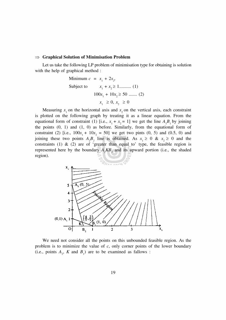
Graphical Solution of Minimisation Problem

Let us take the following LP problem of minimisation type for obtaining is solutionwith the help of graphical method :

Minimum c = x1 + 2x

2,

Subject to x1 + x

2 1.......... (1)

100x1 + 10x

2 50 ....... (2)

x1 0, x

2 0

Measuring x1

on the horizontal axis and x2

on the vertical axis, each constraintis plotted on the following graph by treating it as a linear equation. From theequational form of constraint (1) [i.e., x

1 + x

2 = 1] we get the line A

1B

1 by joining

the points (0, 1) and (1, 0) as before. Similarly, from the equational form ofconstraint (2) [i.e., 100x

1 + 10x

2 = 50] we get two pints (0, 5) and (0.5, 0) and

joining these two points A2B

2 line is obtained. As x

1 0 & x

2 0 and the

constraints (1) & (2) are of ‘greater than equal to’ type, the feasible region isrepresented here by the boundary A

2KB

1 and its upward portion (i.e., the shaded

region).

We need not consider all the points on this unbounded feasible region. As theproblem is to minimize the value of c, only corner points of the lower boundary(i.e., points A

2, K and B

1) are to be examined as fallows :

20

Corner Points Co-ordinates (x, y) Values of objective function

A2

(0, 5) C = 1 0 + 2 5 = 10

K4 5

,9 9

? ?? ?? ?

C = 149

59

149

[solving equational forms

of constraints (1) & (2)]

B1

(1, 0) C = 1 1 +2 0 = 1

We see that the value of C is minimum at B1 and consequently the optimum

solutions are :

x1 = 1, x

2 = 0 and c = 1.

2.4.2 Exceptional cases in LP Solution

Though in practice such small problems involving only two decision variables areusually not encountered, the graphical procedure is useful to illustrate some of the basicconcepts used in solving LP problems. Further, with the help of graphical method wecan clearly explain the exceptional cases that may arise in L.P. solution. These exceptionalcases are explained one by one as follows.

Alternative Optima : In some LP problems there may exist moe than one set ofoptimum solutions. Graphically this situation will arise when the objective functionhappens to be parallel to any of the constraints. Alternatively, if on two corner pointsthe value of the objective function is equally optimized, all the points on the linesegment having these two corner points represent alternative optima.

Unbounded Solution : In some LP problems it is passible to find betterfeasible solution continuously improving the objective function values. Inmaximimisation case this situation arises if there remains no upper boundary in thefeasible region specially in the direction of increasing values of the objective function.Similarly, in minimisation LP problem, this situation of unbounded solution arisesif there is no lower boundary in the feasible region in that direction where valuesof the objective function can be decreased continuously. In reality LP problemsbecome unbounded due to omission of certain constraints by mistake.

Infeasible Solution : Infeasible solution implies that in the given LP problemthere is no solution which satisfies all the constraints. This situation will arise when

21

for a given problem no feasible region can be identified. If in an LP problem thereare only two constraints—one is ‘’ type and other is ‘’ type, the feasible regiondoes not exist and we get infeasible solution.

Degeneracy : In the feasible region optimally is achieved by examining onlythe corner points. Further, a corner point is cropped up from the intersection ofeither (i) two constraints or (ii) one constraint and one axis or (iii) two axes. Butif in any of these three cases to produce corner point unnecessarily one additionalconstraint remains present, this situation of degenracy will arise. Actuallydegeneracy creates no practical difficulty in obtaining optimum solution; this willlead to the conceptual inconvenience. The meaning of degeneracy will be explainedlater on.

2.5 Technical Issues in Linear Programming

If the number of decision varaibles are more than two, the graphical methodfails to obtain the optimum solution. In that case algebraic method (known assimple method) would be required. Before explaining the simplex method, sometechnical issues related to the linear programming are analysed in this section oneby one.

2.5.1 Different Forms of LP

LP problems can be represented in various forms as explained below :

General Form : Satisfying the necessary assumption of the LP, if a given problemis represented in the form of a mathematical model, that form is known as generalform. An example of general form is given below :

Example 1. Maximize z = 4x1 + 2x

2 +3x

3,

subject to 7x1 + 3x

2 + x

3 150 ....... (1)

4x1 + 4x

2 + 2x

3 200 ....... (2)

3x1 - 6x

2 - 4x

3 = – 100 ....... (3)

x1, x

2, x

3 0.

22

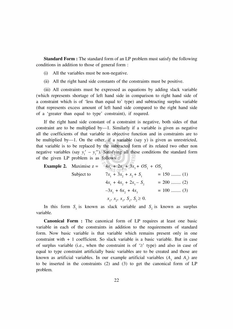
Standard Form : The standard form of an LP problem must satisfy the followingconditions in addition to those of general form :

(i) All the variables must be non-negative.

(ii) All the right hand side constants of the constraints must be positive.

(iii) All constraints must be expressed as equations by adding slack variable(which represents shortage of left hand side in comparison to right hand side ofa constraint which is of ‘less than equal to’ type) and subtracting surplus variable(that represents excess amount of left hand side compared to the right hand sideof a ‘greater than equal to type’ constraint), if requred.

If the right hand side constant of a constraint is negative, both sides of thatconstraint are to be multiplied by—1. Similarly if a variable is given as negativeall the coefficients of that variable in objective function and in constraints are tobe multiplied by—1. On the other, if a variable (say y) is given as unrestricted,that variable is to be replaced by the subtracted form of its related two other nonnegative variables (say y

1 – y

1). Satisfying all these conditions the standard form

of the given LP problem is as follows :

Example 2. Maximise z = 4x1 + 2x

2 + 3x

3 + OS

1 + OS

2

Subject to 7x1 + 3x

2 + x

2 + S

1= 150 ........ (1)

4x1 + 4x

2 + 2x

3 – S

2= 200 ........ (2)

–3x1 + 6x

2 + 4x

3= 100 ........ (3)

x1, x

2, x

3, S

1, S

2 0.

In this form S1

is known as slack variable and S2

is known as surplusvariable.

Canonical Form : The canonical form of LP requires at least one basicvariable in each of the constraints in addition to the requirements of standardform. Now basic variable is that variable which remains present only in oneconstraint with + 1 coefficient. So slack variable is a basic variable. But in caseof surplus variable (i.e., when the constraint is of ‘’ type) and also in case ofequal to type constraint artificially basic variables are to be created and those areknown as artificial variables. In our example artificial variables (A

1 and A

2) are

to be inserted in the constraints (2) and (3) to get the canonical form of LPproblem.

23

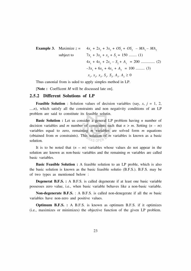
Example 3. Maximize z = 4x1 + 2x

2 + 3x

3 + OS

1 + OS

2 – MA

1 – MA

2

subject to 7x1 + 3x

2 + x

3 + S

1 = 150 ........ (1)

4x1 + 4x

2 + 2x

3 – S

2 + A

1 = 200 .............. (2)

–3x1 + 6x

2 + 4x

3 + A

2 = 100 ......... (3)

x1, x

2, x

3, S

1, S

2, A

1, A

2 0

Thus canonial from is uded to apply simples method in LP.

[Note : Coefficent M will be discussed late on].

2.5.2 Different Solutions of LP

Feasible Solution : Solution values of decision variables (say, x, j = 1, 2,....n), which satisfy all the constraints and non negativity conditions of an LPproblem are said to constitute its feasible solutin.

Basic Solution : Let us consider a general LP problem having n number ofdecision variables and m number of constraints such that n > m. Setting (n – m)variables equal to zero, remaining m variables are solved form m equations(obtained from m constraints). This solution of m variables is known as a basicsolution.

It is to be noted that (n – m) variables whose values do not appear in thesolution are known as non-basic variables and the remaining m variables are calledbasic variables.

Basic Feasible Solution : A feasible solution to an LP proble, which is alsothe basic solution is known as the basic feasible solutio (B.F.S.). B.F.S. may beof two types as mentioned below :

Degenerat B.F.S. : A B.F.S. is called degenerate if at least one basic variablepossesses zero value, i.e., when basic variable behaves like a non-basic variable.

Non-degenerate B.F.S. : A B.F.S. is called non-denegerate if all the m basicvariables have non-zero and positive values.

Optimum B.F.S. : A B.F.S. is known as optimum B.F.S. if it optimizes(i.e., maximizes or minimizes) the objective function of the given LP problem.

24

2.5.3 Fundamental Theorem of LP

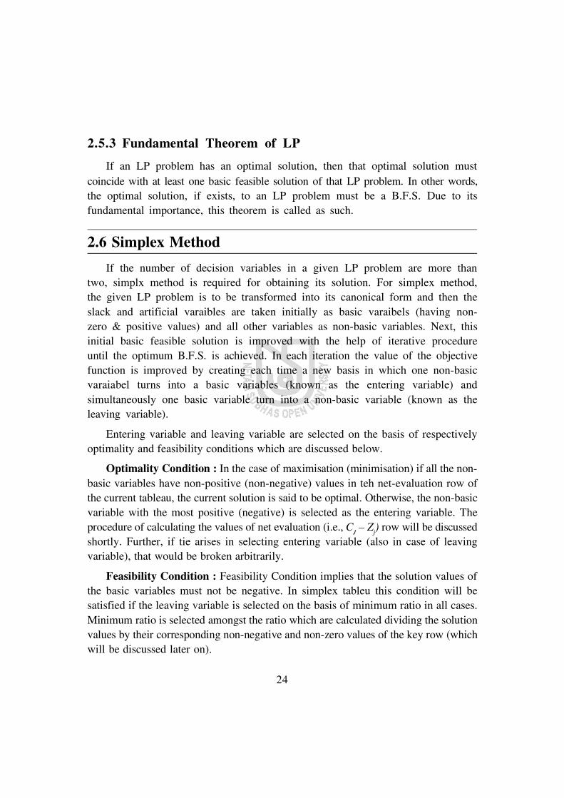
If an LP problem has an optimal solution, then that optimal solution mustcoincide with at least one basic feasible solution of that LP problem. In other words,the optimal solution, if exists, to an LP problem must be a B.F.S. Due to itsfundamental importance, this theorem is called as such.

2.6 Simplex Method

If the number of decision variables in a given LP problem are more thantwo, simplx method is required for obtaining its solution. For simplex method,the given LP problem is to be transformed into its canonical form and then theslack and artificial varaibles are taken initially as basic varaibels (having non-zero & positive values) and all other variables as non-basic variables. Next, thisinitial basic feasible solution is improved with the help of iterative procedureuntil the optimum B.F.S. is achieved. In each iteration the value of the objectivefunction is improved by creating each time a new basis in which one non-basicvaraiabel turns into a basic variables (known as the entering variable) andsimultaneously one basic variable turn into a non-basic variable (known as theleaving variable).

Entering variable and leaving variable are selected on the basis of respectivelyoptimality and feasibility conditions which are discussed below.

Optimality Condition : In the case of maximisation (minimisation) if all the non-basic variables have non-positive (non-negative) values in teh net-evaluation row ofthe current tableau, the current solution is said to be optimal. Otherwise, the non-basicvariable with the most positive (negative) is selected as the entering variable. Theprocedure of calculating the values of net evaluation (i.e., C

J – Z

j) row will be discussed

shortly. Further, if tie arises in selecting entering variable (also in case of leavingvariable), that would be broken arbitrarily.

Feasibility Condition : Feasibility Condition implies that the solution values ofthe basic variables must not be negative. In simplex tableu this condition will besatisfied if the leaving variable is selected on the basis of minimum ratio in all cases.Minimum ratio is selected amongst the ratio which are calculated dividing the solutionvalues by their corresponding non-negative and non-zero values of the key row (whichwill be discussed later on).

25

With the help of simple examples, the simplex method is illustrated below.

2.6.1 Use of Simplex Method in Maximisation Problem

Let us take the earlier example of LP problem of maximisation type for theillustration of simplex method :

Maximize z = 5x + 6y,

subject to x + y 5,

2x + 3y 12,

x, y 0

Its canonical form is :

Maximize z = 5x + 6y + OS1 + OS

2,

subject to x + y + S1 + OS

2 = 5,

2x + 3y + OS1 + S

2 = 12

x, y, S1, S

2 0.

In order to simplify the handling of the equations in the problem, they can berepresented in a special tabular form known as simplex tableau. The initial simplextableau is as follows :

Simplex Tableau I : Initial Step

Cj 5 6 0 0

Line No. CBj

Basis x y S1

S2

Solution Ratio

L1

0 S1

1 1 1 0 551

=5

L2

0 S2

2 3 0 1 12123

= 4

Zj

0 0 0 0

Cj – Z

j5 6 0 0 Z = 0

The values of Cj row are the coefficients of the variables in the objective

function. The basic varaibles (here slack variables) are written under the column‘Basis’ and the values of C

Bi column denote the contributions of the basic variables

in the objective function. As x and y being non-basic variables are equal to zero,solution of S

1 = 5 and solution of S

2 = 12; those are written under solution

26

column. The main body of the tableu is constructed by taking left hand sidecoefficients of the constraints. The values of Z

j row are calculated multiplying the

values of each column related to a variabel by the corresponding values of CBi

and then summing them together. Subracing the values of Zj from the corresponding

values of Cj, the values of net evaluation row (C

j – Z

j) are computed. From the

initial table it is observed that the net evaluation of y is highest positive. So yis selected as entering variable and its corresponding column is known as keycolumn (marked by vertical arrow). Dividing the values of solution column bythier corresponding values in key column ratios are calculated. As ratio 12

3 islower, S

2 is selected as leaving varaibale and its corresponding row (marked again

by a horizontal arrow) is known as key row. The elemnt which lies in theintersection of key row and key column is known as key element put within acircle). In the next table S

2 will be replaced by y and row operations are to be

performed for that table using the following two formulae :

old key row

New = key element

and New non-key row = old non-key row—New Key row corresponding keycolumn element.

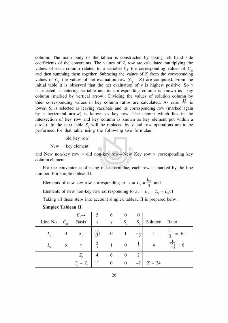
For the convenience of using these formulae, each row is marked by the linenumber. For simple tableau II.

Elements of new key row corresponding to y = L4 = 2

3L

and

Elements of new non-key row corresponding to S1 = L

3 = L

1 – L

41

Taking all these steps into account simplex tableau II is prepared belw :

Simplex Tableau II

Cj 5 6 0 0

Line No. CBj

Basis x y S1

S2

Solution Ratio

L3

0 S1

13e j 0 1 1

3 1113

FHG

IKJ

= 3

L4

6 y 23 1 0 1

3 4123

FHG

IKJ = 6

Zj

4 6 0 2

Cj – Z

j1 0 0 –2 Z = 24

27

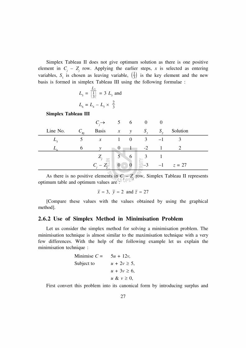
Simplex Tableau II does not give optimum solution as there is one positiveelement in C

j – Z

j row. Applying the earlier steps, x is selected as entering

variables, S1 is chosen as leaving variable, 1

3e j is the key element and the newbasis is formed in simplex Tableau III using the following formulae :

L5 =

L3

13

FHG

IKJ

= 3 L3 and

L6 = L

4 – L

5 2

3

Simplex Tableau III

Cj 5 6 0 0

Line No. CBj

Basis x y S1

S2

Solution

L5

5 x 1 0 3 –1 3

L6

6 y 0 1 -2 1 2

Zj

5 6 3 1

Cj – Z

j0 0 –3 –1 z = 27

As there is no positive elements in Cj – Z

j row, Simplex Tableau II represents

optimum table and optimum values are :

x y z 3, 2 and 27

[Compare these values with the values obtained by using the graphicalmethod].

2.6.2 Use of Simplex Method in Minimisation Problem

Let us consider the simplex method for solving a minimisation problem. Theminimisation technique is almost similar to the maximisation technique with a veryfew differences. With the help of the following example let us explain theminimisation technique :

Minimise C = 5u + 12v,

Subject to u + 2v 5,

u + 3v 6,

u & v 0,

First convert this problem into its canonical form by introducing surplus and

28

artificial variables as follows :

Minimise C = 5u + 12v + 0S1 + 0S

2 + MA

1 + MA

2 ,

subject to u + 2v – S1 + 0S

2 +A

1 + 0A

2 = 5,

u + 3v + 0S1 – S

2 + 0A

1 + A

2 = 6,

u, v, S1, S

2, A

1 & A

2 0.

Here S1 & S

2 denote surplus variables and A

1 & A

2 are the artificial varaibels.

M is defined as an infinitely large number. The rationale for attaching such largecoefficients (+M) to artificial variables lies in the fact that these variables are verylikely to leave the basis as soon as possible. If at least one of them appears inthe solution even with one unit value, the value of the objective function will beinfinitely large in this minimisation problem. This method of assigning a verylarge positive eoefficient to an artificial varaibale in the objective function of aminimisation problem is known as penalty method. It should be noted in thisconnection that in case of maximisation problem the artificial variable (if arises)is penalised in the objective function with -M coefficient (other steps will remainsame).

Next prepare the initial sixplex tableau as in the maximisation problem and inthat tableau basic variables (which remain in the basis) will be those variableswhich have +1 coefficients in the constraints of canonical form and each of whichonly persents in one constraint (i.e, either slackor artificial variables will be thebasic variables in the initial tableau).

Simplex Tableau I

Cj 5 12 0 0 M M

Line No. CBj

Basis u v S1

S2

A1

A2

Solution Ratio

L1

M A1

1 2 –1 0 1 0 5 52 2 5

L2

M A2

1 3 0 –1 0 1 6 63 2

Zj

2M 5M –M –M M M Z = 11 M

Cj – Z

j5-2M 12-5M M M 0 0

The elements in Cj – Z

j row are calculated as before. In case of minimisation

proble, the current solution will be optimum if all the elements in Cj – Z

j row

are non-negative; otherwise, solution is non-optimal and optimality is to be achieved

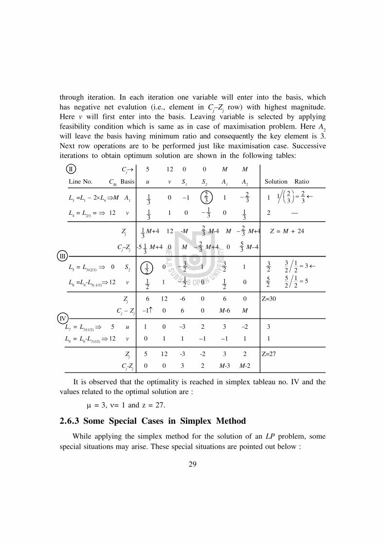
29

through iteration. In each iteration one variable will enter into the basis, whichhas negative net evalution (i.e., element in C

j–Z

j row) with highest magnitude.

Here v will first enter into the basis. Leaving variable is selected by applyingfeasibility condition which is same as in case of maximisation problem. Here A

2

will leave the basis having minimum ratio and consequently the key element is 3.Next row operations are to be performed just like maximisation case. Successiveiterations to obtain optimum solution are shown in the following tables:

II Cj 5 12 0 0 M M

Line No. CBj

Basis u v S1

S2

A1

A2

Solution Ratio

L3 =L

1 – 2L

4M A

113

0 –1 23 1 2

3 1 1 23

23

FH IK

L4 = L

2/3 = v 1

31 0 1

3 0 13

2 —

Zj

13

M+4 12 -M 23 M-4 M – 2

3 M+4 Z = M + 24

Cj–Z

j-5 1

3M+4 0 M – 2

3 M+4 0 53 M–4

III

L5 = L

3/(2/3) S

212

32 3

2 32

32

12

3

L6 =L

4-L

5(-1/3) v 1

2 1

2 12

52

52

12

5

Zj

6 12 -6 0 6 0 Z=30

Cj – Z

j–1 0 6 0 M-6 M

IVL

7 = L

5/(1/2) u

L8 = L

6-L

7(1/2) v 0 1 1 –1 –1 1 1

Zj

5 12 -3 -2 3 2 Z=27

Cj-Z

j0 0 3 2 M-3 M-2

It is observed that the optimality is reached in simplex tableau no. IV and thevalues related to the optimal solution are :

= 3, = 1 and z = 27.

2.6.3 Some Special Cases in Simplex Method

While applying the simplex method for the solution of an LP problem, somespecial situations may arise. These special situations are pointed out below :

30

(i) If any artificial variable remains present in the basis of the final tableau whereoptimality condition is satisifed, then that type of solution is known as in feasiblesolutio. As artificial variable is meaningless and it has no real existence, the optimumsolution with its presene implies infeasible solution.

(ii) By definition, the non-basic variable’s value is taken as zero and thebasic variable’s value is positive. But if basic variable behaves like a non-basicvariable i.e., if the solution value of the basic variable is zero, that problem isknown as degeneracy which may arise either in the final tableau or at the iterativestage.

(iii) If all the elements of key column happen to be either zero and negativeand the current solution is not optimum, then the situation of unbounded solutionarises. In this situation, no ratio can be computed i.e, no entering variable canbe selected, though one basic variable satisfies the conditon to leave the basis. Inthis case solution can be improved indefinitely in the direction of the leavingvariable.

(iv) Another special case in LP problem is the presence of alternative optima.In applying simplex method the situation of alternative optima arise whencorresponding to the final tableau, the net evaluation (i.e, the element in C

j – Z

j

row) of any non-basic variable is zero. If that non-basic variable enters into thebasis, the value of the objective function will nto change and we get anotheroptimum solution.

2.7 Duality in Linear Programming

For every LP problem there is a corresponding opposite problem called thedual problem.The original problem is known as the primal problem. It is sometimeseasier to find the solution of a programming problem by first solving its associateddual problem. The calculation of the dual also allows us to check on the accuracyof the primalproblem. Although every LP problem has a dual problem, theinterpretation and interrelationship of the solutions of the primal and the dual arenot every straight forward. In this last section shall consider the dual formulation,primal-dual relationship and the improtant on uality.

31

2.7.1 Dual Formulation

For the dual formualtion of a primal problem the following steps are to betaken :

1. Transform the primal problem in its standard form

2. For every primal constraint (except non-negative constraints) create one dualvariable.

3. Objective function coefficients of dual variables are the repective right handside constrants of the primal constraints.

4. For each primal variable create one dual constraint whose left hand sidecoefficients are the coefficients of that primal variable in primal constraints (i.e., foreach primal column create one dual row) and whose right hand side constant is thecoefficient of that primal variable in primal objective function.

5. If primal is a maximisation problem, dual will be a minimisation prblem andvice versa.

6. If the dual is of maximisation (minimisation) type, the signs of all dualconstraints are () type.

7. If otherwise nothing is specified, the dual variables are unrestricted innature.

consider the following primal problem :

Maximise Z = 2x1 + 3x

2 + 4x

3

subject to x1

+ x2 + x

3 8,

–2x1

+ x2

– 3x3 –7,

x1

+ 2x2 + 4x

3 = 15

x1, x

3 0 and x

2 is unrestricted.

Replacing x2 by x

2 – x

2 (where x

2 0 and x

2 0) we get its standard form as

follows :

Maximise Z = 2x1 + 3 x

2 – 3x

2 + 4x

3 + 0S

1 + 0S

2

x1 + x

2 – x

2 + x

3 + S

1 + 0S

2 = 8 ........ (1)

2x1 – x

2 – x

2 + 3x

3 + 0S

1 + S

2 = 7 ........ (2)

32

x1 + 2x

2 – 2x

2 + 4x

3 + 0S

1 + 0S

2 = 15 ........ (3)

x1, x

2 , x

2 , x

3, S

1, S

2 0.

In this standard form all the varaibles are non-negatives, constraints are to equalto type and right hand side constants of the constraints are positive. As in the primalproblem there are 3 constraints, we have to crate 3 dual variables, namely y

1, y

2

and y3 and following the above mentioned steps the dual problem is :

Minimise C = 8y1 + 7y

2 + 15y

3,

subject to y1 + 2y

2 + y

3 2,

y1 - y

2 + 2y

3 3,

–y1 + y

2 - 2y

3 –3,

y1 + 3y

2 + 4y

3 4,

y1 0,

y2 0,

y3 is unrestrocted.

Combining second and third constraint the final form of the dual problem is:


2 + ...

subject to y1 + 2y

2 + ...2.

y1 – 2y

3 – 3,

y1 + 3y

2 + 4 4,

y1 y

2 0 and y

3 is unrestricted.

It can be checked that the dual of the dual is the primal problem. For that,first consider the standard form of the dual problem as follows (replacing y

3 by

y3

– y3) :


2 + 15y

3 – 15y

3 + 0S

1 + 0S

3,

subject to y1 + 2y

2 + y

3 – y

3 – S

1 + S

2 = 2,

y1 – y

2 + 2y

3 – 2y

3 + 0S

1 + 0S

3 = 3,

y1 + 3y

2 + 4y

3 – 4y

3 + 0S

1 – S

3 = 4,

y1, y

2, y

3 , y

3 , S

1 and S

2 0.

33

To maintain parity let us assume that the variables related with first, second andthird constraints are x

1, x

2 and x

3 rrspectively. Therefore, the dual of this dual

problem is :


2 + 4x

3,

subject to x1 + x

2 + x

3 8,

2x1 – x

2 + 3x

3 7,

x1 + 2x

2 + 4x

3 15,

–x1 – 2x

2 – 4x

3 –15,

–x1 0,

–x3 0 and x

2 is unrestricted.

Combining thrid and fourth constraints, we get its final dual form as follows :


2 + 4x

3,

subject to x1 + x

2 + x

3 8,

2x1 – x

2 + 3x

3 7,

x1 + 2x

2 + 4x

3 =15,

x1, x

3 0 and x

2 is unrestricted.

This is nothing but the primal problem.

2.7.2 Important Theorems on Duality

Apart from the throrem that the dual of the dual is a primal problem, thereare also many other important theorems on duality, which are stated bleow (withoutgiving any proof) :

(i) If either the primal or the dual problem has a finite optimum solution,then the other problem has also a finite optimum solution.

(ii) The optimal values of the primal and the dual objective functions arealways identical.

(iii) If the primal (dual) has an infeasible solution, it dual (primal) solutionwill be unbounded.

34

(iv) If a certain decision variable in a linear programing problem is optimallynon-zero, the corresponding dummy variable (slack or surplus) in the counterpartprogramming problem must be optimally zero. On the other, if a certain dummyvariable (slack or surplus) in a linear programming problem is optimally non-zero,the corresponding decision variable in the counterpart programming problem mustbe optimally zero. Thereofre, at the optimal stage, the product between the dual(primal) decision variable and its related primal (dual) dummy variable is alwaysequal to zero. This theorem is known as complementary slackness theorem.

(v) At the non-optimal stage, the value of the primal objective function is less(greater) than the value of the dual objective function if the primal problem is theproblme of maximisation (minimisation).

2.7.3 Primal-Dual Relationship

Already some primal-dual relations are pointed out in temrs of the theorems in thepreceding sub-section. Along with those, some other relations can be established withthe help of example as follows:

Primal problem Dual problem

Max. Z = 5x + 6y, Min. C = 5u + 12v,

sub. to x + y 5, sub. to u + 2v 5,

2x + 3y 12, u + 3v 6,

x, y 0 u, v 0

[These two problems have alrady been solved in section 2.6]

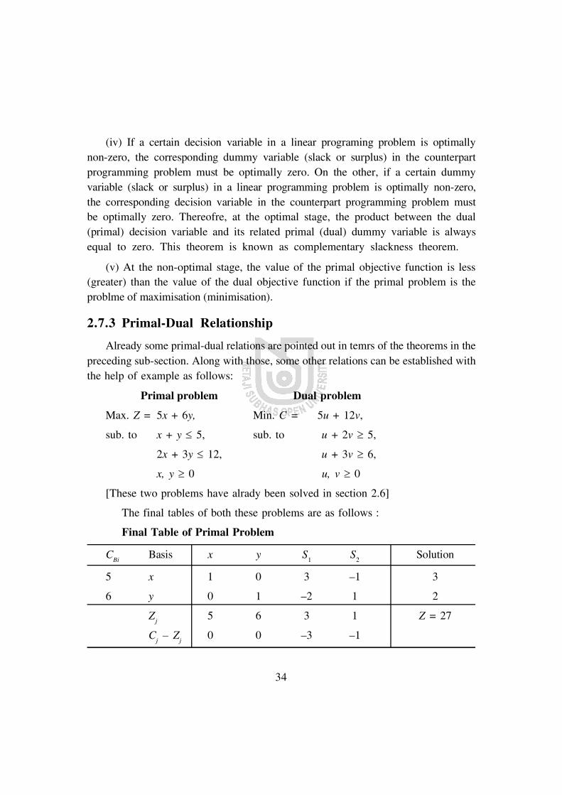
The final tables of both these problems are as follows :

Final Table of Primal Problem

CBi

Basis x y S1

S2

Solution

5 x 1 0 3 –1 3

6 y 0 1 –2 1 2

Zj

5 6 3 1 Z = 27

Cj – Z

j0 0 –3 –1

35

Final Table of Dual Problem

CBj

Basis u v t1

t2

A1

A2

Solutuion

5 u 1 0 –3 2 3 –2 3

12 v 0 1 1 –1 –1 1 1

Zj

5 12 –3 –2 3 2 C = 27

Cj – Z

j0 0 3 2 M-3 M-2

[where t1 and t

2 denote dual surplus variales].

Comparing these two optimal tables it is observed that

(i) z = C = 27 [i.e., optimal solutions of primal and dual objective functions aresame].

(ii) x = 3 = element of Cj – Z

j row related to t

1 column.

similarly y = 2 = element of Cj – Z

j row related to t

2 column. [i.e., the optimum

values of the primal variables can be obtained from the net evaluations of the relateddual slack or surplus variables (ingnoring sign) or artificial variables (in case of ‘=’type constraints, putting M = 0 and then ignoring sing)].

(iii) u = 3 = magnitude of the element of Cj – Z

j row related to the S

1

column. Similarly, v =1 = magnitude of the element of Cj – Z

j row related to

the S2 column.

[i.e., The optimum values of the dual varaibles can similarly be obtained from thenet evaluations of the related primal dummy variables ignoring sing and putting M =0, requried].

(iv) Further it is observed that

x = 3 and t 1

= 0 x .t 1

= 0

y = 2 and t 2

= 0 y .t 2

= 0

u = 3 and s 1 = 0 u .s 1

= 0

v = 1 and s 2 = 0 v .s 2

= 0

All these establish the complementary slackness theorem. It should bementioned in this connection that if x and y represent two prducts and primalconstraints are the resource constraints then u and v (i.e., the dual variables)

s

36

represent the shadow prices of the resources (say, labour, capital) and dual objectivefunction denotes the total cost of using resources in the production procesws. Inthis way one can also given the economic interpretation of duality.

2.8 Summary

Let us conclude the analysis of Linear Programming in the following lines.The LP has wide applications, specially in allocation related descision makingproblems each of which can be formulated in form of a linear objective functionand some linear constraints. If the number of decison variables areonly two, thegraphical method can be applied to solve an LP problem, But the simplex methodcan be applied to solve the LP problem haivng any number of decision variables.In simplex method through limited number of iterations optimal solution of an LPproblem is worked out from non-optimal situation, maintaing always the feasibilitycondition. Apart from its usual nature, the solution of an LP problem may beunbounded, infeasible, multiple (i.e., not unique) and irregular (i.e., basic variablemay take zero value which is known as degeneracy). An LP problem can alsobe transformed into its dual form which has speical economic meaning. Furtherm,as primal and dual solutions are very much related, one can be used to obtainthe other.

2.9 Exercise

1. A furniture maker has 6 units of wood and 28 hours of free time, bywhich he will make decorative screens. Two models are to be produced by thefurniture maker. He estimates that model I requires 2 units of wood and 7 hoursof time for one unit production, while one unit of model II requres 1 unit of woodand 8 hours of time. The prices of the models are Rs. 120 and Rs. 80 respectively.How many screens of each mnodel should the furnitues maker assemble if thewishes maximize his sales revenue?

2. Solve the problem (1) using graphical method.

3. Solve the following LP problem using simplex method :

37

Max. Z = x1 + 9x

2 + x,

sub to x1 + 2x

2 + 3x

3 9,

3x1 + 2x

2 + 2x

3 15,

x1, x

2, x

3 0.

4. Solve the following LP problem using simplex method :

Max. Z = 5x1 + 2x

2,

sub t0 6x1 + x

2 6,

4x1 + 3x

2 12.

x1, x

2 0.

5. Solve the following :

Minimize C = 2x1 + 7x

2,

subject to 1

2

1 2 8,

0 1 3

x

x

? ?? ? ? ??? ?? ? ? ?

? ? ? ?? ?

x1, x2 0.

6. Write the dual for the following LP problem :

Max Z = 2x1 + 4x

2

sub to x1 + x

2 8,

x1 – x

2 5

2x1

+ 3x2

=16

x1

+ 3x2 14,

x1

, x2 0

Show that the dual of the dual is primal. Solve the dual problem and findout the optimal values of the primal decision variables.

7. Give the economic interpretaion of the duality. State the important theoremson duality.

8. Write a short note on the special cases of simplex method.

38

2.10 References

1. V. K. Kapoor : Operations Research, Sultan Chand & Sons, New Delhi.

2. Paik : Quantitative Method for Managerial Decisions, Tata McGraw HillCo. Ltd.

3. Gupta, ManMohan & Swarup : Operations Research, Sultan Chand & Sons,New Delhi.

4. Philips, Ravindra and Solberg : Operations Research : Principles and Pratice,Wiley, New York.

39

Unit 3 p Transportation Problem

Structure

3.0 Objectives

3.1 Introduction

3.2 Mathematical Formulation of Transportation Problem

3.3 Transportation Methods for finding Initial Solution

3.3.1 North West Corner Method

3.3.2 Least Cost Method

3.3.3 Vogel’s Approximation Method (VAM)

3.4 Transportation Algorithm for Obtaining Optimum Solution

3.4.1 Test for Optimality

3.4.2 Dual of the Transportation Model

3.5 Degeneracy in Transportation Problem

3.6 Summary

3.7 Exercises

3.8 References

3.0 Objectives

The objectives of this unit are to discuss the following topics which will help tosolve many real life problems related to transportation :

l Nature of a transportation problem

l Transportation Alogirithm for finding initial solution

l Transportation Algorithm for obtaining optimum solution

l Degeneracy in transportation solution.

40

3.1 Introduction

Transportation problem refers to the problem of determining the minimum costfor distributing a product from several supply points to several demand points.Practically business and manufacturing units have to decide how many units ofa product should be transported from different origins (i.e., factories, plants,warehouses etc.) to different destinations (i.e., markets, sales depots, etc.) so thatthe total tranportation cost becomes the minimum.

Transportation problem is a special type of linear Programming problem anddue to its special character a separate algorithm (known as transportation algorithm)has been developed on the assumption that transportation routes are given. Thisunit mainly covers the mathematical formulation of a typical tranportation problemand the step to be adopted for obtaining its solution in normal situation and alsoin the situation of degeneracy.

3.2 Mathematical Formulation of TransportationProblem

A transportation problem is generally expressed in a tabular form, known astransportation tableau. Transportation tableau representes various transportation costsper unit of product transported from various origins to different destinations. The actualform of the transportation tableau is given below :

41

Transportation TableauDestinations

D1

D2

... Dj ...

Dm

Supplies

O1

C11

C12

C1j

C1m

a1

X11

x12

x1j

X1m

O2

C21

C22

C2j

C1m

a2

X21

X22

X2j

X2m

: :

: :

Origins Ci1

Ci2

Cij

Cim

ai

Oi

Xi1

Xi2

Xij

Xim

: :

: :

Cn1

Cn2

Cnj

Cnm

On

Xn1

Xn2

Xnj

Xnm

an

Demands b1

b2 ...

bj ...

bm

ai b jji

Different symbols used in the above table hae the following meanings :

Cij denotes per unit transportation cost of the product from origin i(i = 1, 2, ...n)

to destination j(j = 1, 2, ... m).

Oi denoted ith origin and D

j denotes jth destination.

aj refers to total supply from ith origin and b

j refers to total demand required for

jth destination.

xij is the decision variable that represents the number of units of the product to be

transported from ith origin to jth destination; Xij may be tiehr zero (if no transportationtakes place) or positive integer (if transportation takes place).

In the transportation problem it is taken that total supply of the product is

equal to the total demand for that product i.e ai b jj im

i jn

FHG

IKJ . This condition is

42

both necessary and sufficient for obtaining basic feasible solution. However in aproblem total supply of the product is greater (lower) than the total deman forthat product, to make them balance a dummy column (row) is to be creted whosedemand (supply) will be difference between a ji

and bjiFurther, due to this

equality of total demand and total supply, in a transportation problem the numberof basic cells (i.e., the cells having positive values of X

ijs.) is m + n – 1 (i.e.,

total column + total row – 1) and all other cells are non-basic cells (i.e., in thesecells, X

ij are zero). It is to be noted that a cell represents the combination of a

supply point and a demand point.

From this transportation tableau, we can give the mathematical formulation of atransportaion problem as follows :

Minimise z =

,1 1

n mC Xij iji j

subject to

,1

mX a jijj

i = 1, 2, ... n [Supply Constraints],

,1

nX bjiji

j = 1, 2, ... m [Demand Constraints],

Xij 0 and integer

Supply constraints should be of ‘’ type and demand constraints should be of‘’ type. But in a transportation problem as the equality between total supply andtotal demand is always mainteained, the constraints are only of ‘equal to’ type.

3.3 Transportation Methods for finding InitialSolution

A solution is known as feasible solution if it satisfies the demand and supplyconditions (i.e., the rim requirements) and if it contains (m + n – 1) number ofbasic cells and rest cells as nob-basic cells. To obtain optimum solution we haveto start from a initial basic feasible solution and then that solution is to beimproved. In this section we discuss three methods for obtaining initial basic

43

feasible solution and the improvement of that initial solution will be explainedin the next section.

3.3.1 North-West Corner Method

Under this method for finding initial solution the following steps are to betaken.

Step 1 : Select the Cell which lies at the north-west corner of the transportationtableau and allocate as much as possible in that cell (i.e., the minimum of demand andsupply corresponding to that cell). After this allocation if demand is exhausted, crossout the column and subtract the allocated amount from the supply of that row to getresidual supply. On the other, after cell allocation if supply is exhausted, cross out therow and compute the residual demand to be met. If the demand and supply correspondingto the north-west corner Cell are equal in amount, then only one of them is crossedout and other’s adjusted quantity will be zero (which is to be treated here as like apositive quantity).

Step 2 : Again select the north-west corner cell among the uncrossed cells andallocate the minimum of demand and supply to that cell. Cross out the satisfied column(or row) and adjust the amount of supply (or demand).

Step 3 : Repeat step 2 until we get single uncrossed row or coumn which allocationsare to be given on the basis of rim conditions.

This method is very simple, but less efficient in the sense that the initialsolution obtained by using this method remains relatively far away from theoptimum solution. Let us consider the following example for the use of thismethod.

Illustration 1.

Suppose a company has factories at four different places (denoted by F1, F

2, F

3,

and F4) which supply warehouses A, B, C, D and E. Monthly factory capacities are

40, 30, 20 and 10 respectively. Monthyly warehouse requrements are 30, 30, 15, 20and 5 respectively. Unit shipping costs (in rupees) are given below. Determine theoptimum distribution to minimize total shipping cost.

44

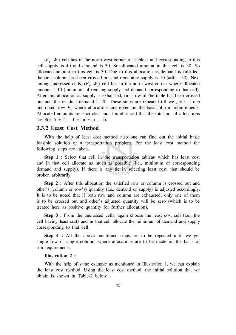
Warehouses

To

From W1

W2

W3

W4

W5

Supply

7 6 4 5 9

F1

40

8 5 6 7 8

F2

30

6 8 9 6 5

Factories F3

20

5 7 7 8 6

F4

10

Demand 30 30 15 20 5 100

This is a balanced transportation problem as total demand = total supply =100. So there is no need of inserting dummy row or dummy column (in whichcell-costs are all taken as zero) in the transportation tableau. Here we like todetermien initial solution of this problem using North-West Corner method andthat is shown in Table-1 below.

Table-1Warehouses

To

From W1

W2

W3

W4

W5

Supply7 6 4 5 9

F1

30 10 40 10 II8 5 6 7 8

F2

20 10 30 10 IV6 8 9 6 5

Factories F3

5 15 20 15 VI5 7 7 8 6

F4

5 5 10Demand 30 30 15 20 5 100

20 5 5

I II V

45

(F1, W

1) cell lies in the north-west corner of Table-1 and corresponding to this

cell supply is 40 and demand is 30. So allocated amount in this cell is 30. Soallocated amount in this cell is 30. Due to this allocation as demand is fulfilled,the first column has been crossed out and remaining supply is 10 (=40 – 30). Nextamong uncrossed cells, (F

1, W

2) cell lies in the north-west corner where allocated

amount is 10 (minimum of remaing supply and demand corresponding to that cell).After this allocation as supply is exhausted, first row of the table has been crossedout and the residual demand is 20. These steps are repeated till we get last oneuncrossed row F

4 where allocations are given on the basis of rim requirements.

Allocated amounts are encircled and it is observed that the total no. of allocationsare 8(= 5 + 4 – l = m + n – 1).

3.3.2 Least Cost Method

With the help of least cost method also one can find out the initial basicfeasible solution of a transportation problem. For the least cost method thefollowing steps are taken.

Step 1 : Select that cell in the transportation tableau which has least costand in that cell allocate as much as possible (i.e., minimum of correspondingdemand and supply). If there is any tie in selecting least cost, that should bebroken arbitrarily.

Step 2 : After this allocation the satisfied row or column is crossed out andother’s (column or row’s) quantity (i.e., demand or supply) is adjusted accordingly.It is to be noted that if both row and column are exhausted, only one of themis to be crossed out and other’s adjusted quantity will be zero (which is to betreated here as positive quantity for further allocation).

Step 3 : From the uncrossed cells, again choose the least cost cell (i.e., thecell having least cost) and in that cell allocate the minimum of demand and supplycorresponding to that cell.

Step 4 : All the above mentioned steps are to be repeated until we getsingle row or single column, where allocations are to be made on the basis ofrim requirements.

Illustration 2 :

With the help of same example as mentioned in Illustration 1, we can explainthe least cost method. Using the least cost method, the initial solution that weobtain is shown in Table-2 below :

46

Table-2Warehouses

To

From W1

W2

W3

W4

W5

Supply

7 6 4 5 9

F1

5 15 20 40 25 5

8 5 6 7 8F

20 30 30 0

6 8 9 6 5

Factories F3

15 5 20 15

5 7 7 8 6

F4

10 10

Demand 30 30 15 20 5 100

II I III IV

In (F1, W

3) cell, cost is lowest and so in that cell first allocation is given to

the amount of 15. As demand is fulfilled due to this allocation, the correspondingcolumn is crossed out and the remaining supply is 25. Next least cost is 5 whichis observed in four cells; among them (F

2, W

2) cell is arbitrarily chosen for

allocation to the amount of 30. Due to this allocation, both demand and supplyare exhausted. But here column is crossed out and the remaining supply is takenas zero. Similarly in third time, (F

1, W

4) cell is chosen and in that cell maximum

possible allocation is 20. So column foru is to be cross out and the adjustedsupply corresponding to F

1 is 5. Next (F

3, W

5) cell is selted for allocation and

consquently fifth column is crossed out. Lastly in the cells of first columnallocations are given on the basis of rim requirements. Taking zero allocation intoaccount in (F

2, W

1) cell, here also the total number of basic cells are 8.

3.3.3 Vogel’s Approximation Method (VAM)

It is observed that the VAM is most efficient method for obtaining initialbasic feasible solution. This method is discussed step wise as follows :

Step 1 : Calculate penalities of all rows and columns. Penalty of a row (orof a column) is the positive difference between two least costs in that row (orthat column). Among the calculated penalities of rows and columns select the

47

highest one (tie is to be broken here arbitrarily) for allocation in the correspondingrow /column.

Step 2 : Allocation is made in the least cost cell of the row/column correspondingto which the penalty is highest. Due to this allocation if row condition is satisfied (i.e.,supply is exhausted), row is crossed out or if column condition (i.e., demand requirement)is fulfilled, column is crossed out or if both are satisfied any one of them is crossedout and other;s quantity is adjusted accordingly.

Step 3 : For the uncrossed rows and columns again calculate the penalities andfollow the above mentioned steps repeatedly until we get either single row or singlecolumn, where allocatins are to be determined on the basis of rim conditions.

In this way we shall get the initial solution having (m + n – 1) basic cells.

Illustrations 3 :

With the help of the same example of illustration 1 we explain all these steps ofthe vogel’s approximation method and the calculation along with allocations are shownin the following Table-3 :

Table-3Warehouses

ToFrom W1 W2 W3 W4 W5 Supply

7 6 4 5 9 25 5F1 5 15 30 40 I I I I I IV

8 5 6 7 8 0F2 0 30 30 1 2 1 0 0

6 8 9 6 5 15

Factories F 3 15 5 20 1 1 1 1 15 7 7 8 6 (orbitarity chosen)

F4

10 10 1 1 1 1 1Demand 30 25 30 15 20 5 100

1 1 2 1 11 1 1 1

Penalties 1 II I 1 11 III 11 1

V

48

In the first round, among the calculated penalties, the penalty of W3 column

is highest (i.e.,2) and in that column as (F1, W

3) cell has the least cost, allocation

(to the amount of 15) is given in that cell. Consequently, column three is crossedout and the remaining supply of F

1 is 25. Again the penalties are calculated and

in this second round F2 row having highest penality is chosen for allocation. In

(F2, W

2) cell cost is least and so in that cell allocation is given as much as

possible (i.e., 30); crossing out the column (related to W2) the remaining supply

of F2 is zero. All these steps are takn repeatedly to allocate successively in cells

(F1, W

1) and (F

3, W

5) to the amounts of 5 and 5 respectively. Lastly in the cells

of first column allocations are made on the basis of rim conditions. Here also,the number of basic cells are 8(i.e., m + n – 1 = 5 + 4 – 1).

To obtain optimum solution one can start from any of these three initial solutionswhich are obtained by applying three methods (namely, North-West corner method,least cost method and VAM).

3.4 Transportation Algorithm for Obtaining OptimumSolution

After obtaining the initial basic feasible solution of a transportation problem,the optimality of that solution is checked. If the solution is found to be non-optimal, that solution is improved through reallocation (with the help of loopformation) until the optimality of the current solution is reached. All these arediscussed here.

3.4.1 Test for Optimality

For checking the optimality of the current basic feasible solution, u – v method(alternatively known as Modi method) is applied as follows :

For the ith row ui (i = 1, 2, ... n) and for the jth column v

j (j = 1, 2, m)

are to be calculated using the following formula corresponding to only basic cells[say, (i, j) th basic cell] :

uj + v

j = c

ij

Here number of unknowns uis and v

js = m + n. But the number of equations

49

= number of basic cells = m + n – 1. That’s why, any one vj or any one u

i is

taken arbitrarily as zero and that will not affect the net evaluations (similar to LPP)of the non-basic cells.

The net evaluations of the non-basic cells [say, (p, q)th non-basic cell] are calculatedusing the following formula :

Net evaluation of (p, q)th non-basic cell = dpq

= Cpq

– (up + v

q).

If all the net evaluations of the non-basic cells are zero or positive, the currentsolution is optimum. Otherwise the current solution is non-optimal and there remainsthe scope for further improvement of the solution through reallocation.

3.4.2 Dual of the Transportation Model

Rationality behind ‘u – v’ or Modi (modified distribution) method can beexplained on the basis of (i) dual formulation of a transportation prblem and (ii)the complementary slackness theorem (which has already been discussed in relationof Linear Programming).

Let us consider the mathematical form of the generalised transportation problem(having m destinations and n origins) as follows :

Minimize z =

,1 1

n mC Xij iji j

subject to 1

nX aij ij

[i = 1, 2, ... n] : Supply Constraints,

1

nX bjiji

[j = 1, 2, ...m] Demand Constraints & Xijs 0

Let the dual variables be

ui for the ith supply constraint (i = 1, 2, ... n)

and vj for the jth demand constraint (j = 1, 2, ... m).

Therefore, the dual formulation of a generalised transpoprtation problem is:

Maximize v =

. ,1 1

n ma u b vj ji ii j

50

Subject to ui + v

j C

ij for all i, j and u

j, v

j are all unrestricted.

Now from complementary slackness theroem we know that the optimum value ofthe primal variable X its corresponding dual slack = 0. For any (i, j) th basic cell asX

ij > 0, its corresponding dual slack = 0. This implies that its corresponding dual

constraint will be of euality type i.e.,

uj + v

j = C

ij

Again for any (p, q)th non-basic cell, Xpq

= 0. Therefore, according tocomplementary slackness theorem its corresponding dual slack 0 i.e.,

up + v

q > C

pq (when dual slack is negative)

or up + v

q = C

pq (when dual slack is zero)

or, up + v

q > C

pq (when dual slack is positive).

Now up denotes the contribution (or shadow price or locational rent) of the pth

origin and vq denotes the contribution (or shadow price) of the qth destination.

If imputed total contribution > cost

i.e., up + v

q > C

pq i.e., C

pq – (u

p + v

q) < 0

i.e., dpq

< 0, it is profitable to reallocate in the (p, q) th non-basic cell. Otherwise,no reallocation is profitable. These are the conditions on the basis of which ‘u – v’method has been developed.

3.4.3 Loop in Transportation Table

If the net evaluations of the non-basic cells are not all euqal to zero or positive,the current solution can be improved through reallocation. Reallocation implies onebasic cell will turn into a non-basic one and one non-basic cell will turn into a basicone. That non-basic cell will turn into a basic one (i.e., will get positve allocation)whose net-evaluation is negative and highest in magnitude (in case of tie, that is brokenarbitrarily).

The leaving basic cell (i.e., the basic ell which will turn into non-basic) is determinedon the basis of loop formation. A loop is constructed through horizontal and vertical(not diagonal) lines which passes through the cells of the transportation tableau. Further,loop is formed starting from that non-basic cell which will get new positive allocationand ending to that non-basic cell. In all other corner points of the loop there must bebasic cells. It is to be noted that for each non-basic cell, there is only one loop (i.e.,loop is unique).

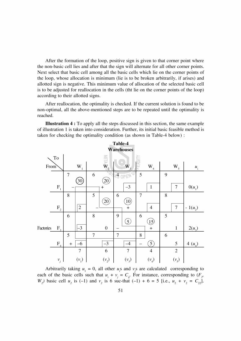
51

After the formation of the loop, positive sign is given to that corner point wherethe non-basic cell lies and after that the sign will alternate for all other corner points.Next select that basic cell among all the basic cells which lie on the corner points ofthe loop, whose allocation is minimum (lie is to be broken arbitrarily, if arises) andallotted sign is negative. This minimum value of allocation of the selected basic cellis to be adjusted for reallocation in the cells (tht lie on the corner points of the loop)according to their allotted signs.

After reallocation, the optimality is checked. If the current solution is found to benon-optimal, all the above-mentioned steps are to be repeated until the optimality isreached.

Illustration 4 : To apply all the steps discussed in this section, the same exampleof illustration 1 is taken into consideration. Further, its initial basic feasible method istaken for checking the optimality condition (as shown in Table-4 below) :

Table-4Warehouses

To

From W1

W2

W3

W4

W5

ui

7 6 4 5 930 20

F1

– + –3 1 7 0(u1)

8 5 6 7 820 10

F2

2 – + 4 7 - 1(u2)

6 8 9 6 55 15

Factories F3

–3 0 – + 1 2(u3)

5 7 7 8 6

F4

+ –6 –3 –4 – 5 5 4 (u4)

7 6 7 4 2

vj

(v1) (v

2) (v

3) (v

4) (v

5)

Arbitrarily taking u1 = 0, all other u

is and v

js are calculated corresponding to

each of the basic cells such that ui + v

j = C

ij. For instance, corresponding to (F

2,

W2) basic cell u

2 is (–1) and v

2 is 6 suc-that (–1) + 6 = 5 [i.e., u

2 + v

2 = C

22].

52

After computing all the ujs and v

js, next, the net evaluation of non-basic cells are

calculated uisng the formula dpq

= Cpq

– (up + v

q). For instance, corresponding to

the (F1, W

3) non-basic cell, the net evaluation is –3 [= 4 – (0 + 7) i.e., d

13 = c

13

– (u1 + v

3)]. It is observed from Table-4 that the current solution is not optimal

as the net evaluations of the non-basic cells are not all non-negative. For theimporvement the current solution of (F

4, W

1) non-basic cell is selected for getting

new allocation (ie.e., entering cell) as this cell has negative net evaluation withhighest magnitude (i.e., – 6). Next to determine the leaving cell among basiccells, the loop is formed (as shown by the bold circuit in Table-4) and alternativelyplus and minus signs are allotted to the cell which lie on the corner points of theloop [starting with plus sign allotted to the non-basic cell (F

4, W

1)]. Next as 5 is

the lowest value of the transported amounts of the basic cells in which negativesigns are allotted, this amount is adjusted for reallocation on the basis of allottedsigns in the cells of the corner points of the loop and the new allocations areshown in Table 5. Due to this new allocation, it is observed that (F

3, W

3) cell

becomes the leaving cell and the allocated amount of (F4, W

4) cell is taken as zero

[because at a time only one basic cell can leave the basis].

Table-5Warehouses

To

From W1

W2

W3

W4

W5

7 6 4 5 9

F1

25 15 –3 1 7

8 5 6 7 8

F2

15 15

6 8 9 6 5

Factories F3

20

5 7 7 8 6

F4

5 0 5

The whole process is to be repeated to obtain its optimum solution.

53

3.5 Degeneracy in Transportation Problem

Degeneracy in transportation problem arises when basic cell behaves like anon-basic cell, i.e., when the allocation of the basic cell is zero. This problemmay arise either in the initial stage or in the interative stage. In the initial stageof obtaining initial basic feasible solution, the degeneracy problem arises if dueto a cell allocation if both total demand and total supply corresponding to thatcell are exhausted at a time. Check Table-2 of illustration 2 and Table-3 ofi l lustration 3; in both these one basic cel l [ (F

2, W

1) cell] gets zero allocation in

the initial stage.

On the other, the degeneracy problem arises in the interative stage [as observed inTable-4 and Table-5 of illustration 4] if in the constructed loop tie is observed inselecting the leaving basic cell which should have minimum allocation with negativeallotted sign. Howver, if the degeneracy problem arises in a transportation problemthen the zero allocation(s) of the basic cell(s) is (are) to be replaced by a very smallpositive quantity such that.

(i) Xij + = X

ij,

(ii) Xij – = X

ij,

(iii) + =

(iv) – =

(v) 0 + = and

(vi)0 – = –

Replacing each zero allocation by , the usual transportation algorithm isapplied to obtain the optimum solution.

Illustration 5. We have started from Table-5 of illustration 4 and replacingzero allocation of cell (F

4, W

4) by , Table-6 is constructed below. Next the

earlier mentioned steps (namely, test of optimality followed by loop formationand reallocation, if required) are applied sequentially in the following tables (withoutgiving any further explanation) to obtain optimum solution.

54

Table-6Warehouses

To

From W1

W2

W3

W4

W5

ui

7 6 4 5 925 15 +

F1

– –3 –5 1 2

8 5 6 7 815 15

F2

2 –2 1 1

6 8 9 6 520

Factories F3

3 6 6 1 –2

5 7 7 8 6 + – 5

F4

5 3 2 0

vj

5 4 5 8 6

Table-7Warehouses

To

From W1

W2

W3

W4

W5

ui

+ – 6 4 5 9 25 15

F1

-3 + 1 0

8 5 6 7 8 15 15

F2

2 –3 1 –16 8 9 6 5

20 +Factories F

3–2 –1 1 – –4 1

5 7 7 8 6 5 + – 5

F4

3 2 5 –2

vj

7 6 7 5 8

55

Table-8Warehouses

Table-9Warehouses

Factories

From

Factories

56

Table-10Warehouses

In Table-10 it is observed that all the net evaluations of the non-basic cells are non-negative. So this solution of Table-10 is optimal. The optimum transported quantititesfrom factories to warehouses are as follows :

Factories Warehouses Transported amount

W1

5

F1

W3

15

W4

20

F2

W2

30

F3

W1

15

W5

5

F4

W1

10

The total cost of transportation = 5 7 + 15 4 +5 20 + 5 30 + 6 15 +5 5 + 10 5 = Rs. 510. The readers can check that the initial solutions obtainedby applying least cost method and VAM are directly optimal. It is observed that if onestarts solution using the VAM, generally few iterations will be required to obtainoptimum solution.

57

3.6 Summary

In a typical transportation problem goods are to be transported from differentorigins to different destinations so that the total cost of transportation is minimised,given (i) the supplies of the origins, (ii) the demands of the destinations and (iii)unit costs of transportation from different origins to different destinations. Thetransportation problem is a special form of linear programming problem. To solvethe transportation problem, a separate algorithm has been developed. In regard totransportation algorithm, first, initial basic feasible solution is found out from thetransportation tableau with the help of either noth-west corner rule or least costmethod or vogel’s approximation method (which is, however, more efficient thanothers). Then the optimality of the solution is checked using ‘u – v’ (i.e., Modi)method. If the solution is not optimal then with the help of loop formationreallocation is made to improve the solution. In this process optimality of thetransportation solution is reached. The usual transportation problem and its solutionmay differ in different directions. Two such special cases, namely unbalancedtransportation and degeneracy in transportation problem have been discussed herebriefly.

3.7 Exercises

1. What is meant by the transportation problem? Give the matehmaticalformulation of the transportation problem.

2. State the basic two theorems of the transportation problem.

3. Briefly discuss the vogel’s Approximation Method for finding initialsolution.

4. What is meant by the Modi Method? Explain the rationality behindthis method with the help of dual formulation of the transportationproblem.

5. Briefly discuss the transportation algorithm. How is this algorithm modified(i) if the transportation problem is unbalanced one and (ii) if degeneracyproblem arises?

58

6. Solve the transportation problem for which the unit transportationcosts, origin availabilities and destination requirements are given in thefollowing table :

Destinations

D E F G H Supply

A 2 11 10 3 7 4

Origins B 1 4 7 2 1 8

C 3 9 4 8 12 9

Demand 3 3 4 5 6

7. Given below is the unit costs array with supplies ai, i = 1, 2, 3, 4 and

demands bj, j = 1, 2, 3, 4, 5.

Markets

Warehouses

M1

M2

M3

M4

M5

ai

5 3 4 4 2

W1

50

9 2 2 3 6

W2

30

Warehouses 6 1 6 1 4

W3

40

4 7 3 5 3

W4

20

bj

40 30 20 50 10

59

3.8 References

1. Sharma : Operations Research, Kedar Nath & Ram Nath.

2. Vohra : Quantitative Techniques in Management, Tata McGrawHill.

3. Kapoor : Operations Research, Sultan Chand & Sons.

4. Paik : Quantitative Method for Managerial Decisions, TataMcGraw Hill.

60

Unit 4 p Assignment Problem

Structure

4.0 Objectives

4.1 Introduction

4.2 Mathematical statement of Assignment Problem

4.3 Hungarian Method of solution

4.4 Maximisation case in Assignment Problem

4.5 Unbalanced Assignment Problem

4.6 Restriction on Assignment

4.7 Travelling Salesman Problem

4.8 Summary

4.9 Exercises

4.10 References

4.0 Objectives

The purpose of this unit is to facilitate knowing the following topics related to theassignment problem :

l Nature of a usual assignment problem

l Assignment algorithm (known as Hungarian Method)

l Some special cases of the usual assignment problem

l Travelling salesman problem and its solution.

After knowing all these one will be able to solve many real life assignment relatedproblems.

61

4.1 Introductions

A usual assignment problem implies the choice of assigning a number ofworkers to an equal number of jobs so that the total cost of performing the jobsis minimised. The assignment problem is a special form of transportation problem.In the assignment problem (i) total number of rows (workers) = total number ofcolumns (jobs), (ii) supply of each row is 1 unit and demand for each columnis also equal to 1 unit and (iii) number of basic variables is equal to the numberof column or row. Due to these special features a separate algorithm (known asHungarian method) has been developed for the solution of an assignment problem.Apart from the usual assignment of workers to the jobs, this type of problem isalso observed in case of flight scheduling processing of products, etc. Further, anassignment problem can also be formulated by taking some special cases intoaccount. One such special case is travelling salesman problem. All these issuesrelated to the assignment problem are discussed in this unit.

4.2 Methematical Statement of Assignment Problem

Suppose n jobs are performed by n workers such that (i) one worker canperform only one job and (ii) any worker can perform any job. Further, costs (orunits of time) of doing jobs differ for different workers and here the objectiveis to minimise the total cost (or time) incurred for completing the jobs. Liketransportation problem, assignment problem can also be represented with the helpof the following table :

62

Assignment Table

Jobs

Workers J1

J2

... Jj

... Jn

Supplies

C11

C12

Cij

C1n

W1

1

X11

X12

X1j

X1n

C21

C22

C2j

C2n

W1

1X

21X

22X

2jX

2n

: :

: :

Ci1

C12

Cij

Cin

W1

1

Xi1

Xi2

Xij

Xin

: :

: :

Cn1

Cn2

Cnj

Cnn

W1

1X

n1X

n2X

njX

nn

Demands 1 1 1 1 n

Where Cij denotes cost of doing jth job by ith worker and X

ij is the variable

corresponding to (i, j)th cell which is equal to 1(0) when jth job is performed (notperformed) by ith worker; i, j = 1, 2, ... n.

From this assignment table we can easily represent the assignment problem in thefollowing mathematical form :

Minimize C =

,1 1

n nC Xij iji j

Subject to

1,1

nXijj

i = 1, 2, ... n [supply constraints]

1,1

nXiji

j = 1, 2, ... n [demand constraints]

and Xij = 0 or 1 (as defined earlier).

63

4.3 Hungarian Method of Solution

For the solution of an assignment problem D. Konig (resident of Hungary)has developed an algorithm which is known as Hungarian method. The steps ofthis method are pointed out below.

Step 1. : Prepare the table (as mentioned earlier) for the given assignmentproblem and this table will be of the form of square matrix having equal numberof rows and columns. In each cell of this table, cost of assignment is given.

Step 2 : Apply the row operation and then the column operation. Therow operation means that the minimum cost of each row is subtracted from allother costs of that row so that in each row at least one zero is observed. Similarly,column operation implies the subtraction of minimum cost of each column fromall other costs of that column by which at least one zero is cropped up in eachcolumn.

Step 3 : Next draw the minimum number of vertical and horizontal (notdiagonal) lines to cross out all the zeros in the assignment table. If the minimumnumber of these lines is equal to the order (i.e., number or rows) of the matrix,the table is ready for getting optimum solution. Otherwise, go to step 4.

Step 4 : Select the lowerst cost amongst the uncrossed costs on the table(after adopting step 2 and step 3). This lowest cost is to be (i) added with thosecosts which are in the junction of vertical and horizontal lines and (ii) subtractedfrom all uncrossed costs; all other costs will remain unchanged.

Step 5 : Repeat step 3 and step 4 until the optimality condition issatisfied. Here optimality condition implies the equality between the number ofminimum lines required to cross zero and the order of the matrix. After thefulfillment of the optimality condition, final assignments are to be determined onthe basis of following rules which may also be used for drawing the minimumnumber of lines to cross out all the zeros :

Rule 1 : Check all the rows one by one and select those rows each ofwhich has single zero. Make assignments on the basis of those single zeros and

64

in each time after determining assignment (denoted by tick mark) draw verticalline (to cross out all zeros of the corresponding column).

Rule 2 : After completing the row checking, examine all the columns oneby one and select those columns each of which has single zero. Make assignmenton the basis of those single zeros and in these cases after making assignmentsdraw horizontal lines (to cross out zeros of the corresonding rows).

Rule 3 : Repeat the above two rules sequentially until all the assignments aredetermined. However, if all the jobs cannot be assigned on the basis of selecting singlezeros, then arbitrarily give assignment to any cell containing uncrossed zero and drawvertical and horizontal lines through theat cell. After this arbitrary choice again followthe above rules.

If rule 3 is required for determining assignment, it signifies the existence of multiplesolutions because in that situation there remains the choice of alternative assignment.With the help of an example we can explain the Hungarian method.

Illustration 1.

A firm employes typists on hourly piece-rate basis for their daily work. There arefive typists and their charges and speed are different. According to an earlierunderstanding only one job is given to one typist and the typist is paid for a full houreven if he works for a fraction of an hour. Find the least cost allocation for thefollowing data :

Typist Rate per hour No. of pages Job No. of Pages(Rs) typed/hour

A 5 12 P 199

B 6 14 Q 175

C 3 8 R 145

D 4 10 S 298

E 4 11 T 178

Solution : Applying step 1 of the Hungarian method the following assignmenttable (Table-1) is prepared. The elements of Table-1 represent costs to be incurreddue to assignment of different jobs to different typists. For instance, to perform jobP by employing typist A, cost = (199 12) 5 = (17 approximately) 5 =Rs. 85.

65

Table-1

Jobs

Typists P Q R S T

A 85 75 65 125 75

B 90 78 66 132 78

C 75 66 57 114 69

D 80 72 60 120 72

E 76 64 56 112 68

Applying the row operation as mentioned in step 2 we get the following reducedcost matrix shown in Table-2.

Table-2

Jobs

Typists P Q R S T

A 20 10 0 60 10

B 24 12 0 66 12

C 18 9 0 57 12

D 20 12 0 60 12

E 20 8 0 56 12

Similarly applying the column operation (step-2), we obtain the reduced cost matrixas shown in Table-3.

Table-3

Jobs

Typists P Q R S T

A 2 2 0 4 0

B 6 4 0 10 2

C 0 1 0 1 2

D 2 4 0 4 2

E 2 0 0 0 2

66

Next step 3 is applied in Table-4 where minimum number of lines (horizontal andvertical) are drawn to cross all the zeros.

Table-4

Jobs

Typists P Q R S T

A 2 2 0 4 0 IV

B 6 4 0 10 2

C 0 1 0 1 2

D 2 4 0 4 2

E 2 0 0 0 2 III

II I

The zero on the basis of which lines are drawn are identified by tick mark and alsosequaence of drawing the lines is marked by Roman numbers. From Table-4 we seethat number of lines is 4 whcih is less than the order of the matrix (5). So step 4 isto be applied and that is shown in Table-5.

Table-5

Jobs

Typists P Q R S T

A 3 2 1 4 0

B 6 3 0 9 1

C 0 0 0 0 1

D 2 3 0 3 1

E 3 0 1 0 2

In Table-5 least cost element 1 (of Table-4) is added to the elements whichare in the junctions and subtracted from the uncrossed elements (keeping all otherdlements in tact). Next to cross all the zeros of Table-5, the minimum number oflines are drawn in Table-6 (just like Table-4).

67

Table-6

Jobs

Typists P Q R S T

A 3 2 1 4 0

B 6 3 0 9 1

C 0 0 0 0 1 III

D 2 3 0 3 1

E 3 0 1 0 2 IV

II I

From Table-6 again we see that the number of lines is less than the order of thematrix. So step-4 is again to be applied selecting 2 as the least cost element. Afterapplying step-4, the adjusted cost matrix is shown in Table-7.

Table-7

Jobs

Typists P Q R S T

A 1 0 1 2 0 III

B 4 1 0 7 1

C 0 0 2 0 3

D 0 1 0 1 1

E 3 0 3 0 4

II IV I V

In Table-7 also step-3 is again applied i.e., to cross all the zeros, minimumnumber of lines are drawn. First three lines are drawn on the basis of singleremaining zero either in row or in column and line (IV) is drawn arbitrarily byslecting zero of (C, Q) cell. Howver, from Table-7 we see that the minimumnumber of lines = the order of the matrix = 5. So here optimality condition issatisfied. Next on the basis of tick marks ( ) in Table-7, we can determine thefollowing optimum assignment (applying step 5) :

68

Jobs Typists

T A

R B

Q C

P D

S E

The total minimum cost of assignment = 75 + 66 = 66 + 80 + 112 =Rs. 399.

The learners can verify that with the same level of cost of Rs. 399, an alternativeoptimum solution for this problem is as follows :

Jobs Typists

T A

R B

Q C

P D

S E

4.4 Maximisation Case in Assignment Problem

In a usual assignment problem either total cost or total time to be requred forcompleting the jobs is minimised. But if the assignment problem is given in termsof productivity or return or profit matrix (in place of cost matrix), the problemwill be of maximisation type. For instance, a company wants to employ foursalesmen to four different markets for selling its product. One salesman is to beemployed for each market. Suppose the efficiency of salesmen differ for differentmarkets and efficiencies of the salesmen measured in terms of their volume ofslaes which are estimated apriori. So here the company will determine theassignment of salesman in such a way that total olume of sales is maximised.

In a maximising type of assignment problem we can use the same Hungarianemthod which is applied to solve an assignment problem of minimisation type by

69

only transforming the efficiency matrix into an opportunity cost matrix.Transformation can be made with the help of any of the following two ways :

(i) Each element of profit or return (i.e., efficiency) matrix is multiplied byminus one and due to this maximisation problem will be changed to a minimisationproblem.

(ii) All the elements of the efficiency matrix are changed by subtracting thosefrom the highest (in value) element of that matrix. With this efficiency matrixwill be turned into an opportunity cost matrix.

Illustration 2 :

Suppose the owner of a small machine shop has four machinists available to assignto jobs for the day. Four jobs are offered with the expected profit in rupees for eachmachinist on each job being as follows. Find the assignment of machinists to jobs thatwill result in a miximum profit.

Jobs

A B C D

1 6.20 7.80 5.00 10.10

Machinists 2 7.10 8.40 6.10 7.30

3 8.70 9.20 11.10 7.10

4 4.80 6.40 8.70 7.70

Solution : In the given profit matrix the highest element is Rs. 11.10 from whichall other unit profits are subtracted and simultaneously replaced to get the followingopportunity cost matrix :

Jobs

A B C D

1 4.90 3.30 6.10 1.00

Machinists 2 4.00 2.70 5.00 3.80

3 2.40 1.90 0 4.00

4 6.30 4.70 2.40 3.40

On this transformed opportunity cost matrix, the Hungarian method is to be appliedto obtain its optimum solution. The readers can check that the optimum solution to thisproblem will be as follows :

70

1 D, 2 B, 3 A, 4 C; ZMax

=Rs. 35.90. One can obtain the samesolution if the given maximisation problem is changed to the minimisation problemwith the following matrix :

Jobs

A B C D

1 –6.20 –7.80 –5.00 –10.10

Machinists 2 –7.10 –8.40 –6.10 –7.30

3 –8.70 –9.20 –11.10 –7.10

4 –4.80 –6.40 –8.70 –7.70

4.5 Unbalanced Assignment Problem

To obtain optimum solution by Hungarian method the necessary conditionis that the assignment problem must be a balanced one i.e., there must be equalnumber of rows (i.e., workers) and equal number of columns (i.e., jobs) in theassignment matrix. But if the cost matrix of the given assignment problem isnot a square matrix having unequal number of rows and columns, the problemis termed as an unbalanced one. In that situation, by incorporating dummy rowor dummy column the assignment problem is transformed into a balanced problemand then the Hungarian method can be applied : More specificily, when thenumber of rows (i.e., workers) are greater than number of columns (i.e., jobs),dummy column is to be added. On the other, if the number of columns (i.e.,jobs) are greater than number of rows (i.e., workers), dummy row is to beadded. All the cell elements of the dummy row of column are considered aszero. After obtaining final solution with the help of the Hungarian method, theassignments related to dummy rows/columns are to be ignored as those have noreal existence. In other words, if there is dummy row, then one job will notbe finished. Similarly, if there is dummy column, then one worker will remainidle. With the help of following two examples the insertion of dummy row/dummy column has explained.

71

Illustration 3 : Suppose a company has 3 machines (denoted by X, Y and Z) toperform four jobs (denoted by A, B, C and D). Each job can be assigned to eachmachine. The following cost matrix is given :

Jobs

A B C D

X 10 7 15 4

Machines Y 12 6 14 3

Z 9 8 17 5

This cost matrix is not a square matrix. Hence this is an unbalanced assignmentproblem and to make it a balance one, dummy row (ie.e, dummy machine) is to beinserted as follows :

Jobs

A B C D

X 10 7 15 4

Machines Y 12 6 14 3

Z 9 8 17 5

Dummy 0 0 0 0

Illustration 4 : Suppose a company faces the problem of assigning fiveworkers to three different jobs. To perform each of the jobs, any one of the fiveworkers is sufficient. The estimated costs of assignment are given in the tablebelow :

Jobs

1 2 3

1 7 6 8

2 6 5 3

Workers 3 4 6 7

4 5 3 4

5 8 9 7

72

This cost matrix also representes an unbalanced assignment problem and totransform it into the balanced form two dummy columns (i.e., two dummy jobs)are to be created as follows :

Jobs

1 2 3 Dummy1

Dummy2

1 7 6 8 0 0

2 6 5 3 0 0

Workers 3 4 6 7 0 0

4 5 3 4 0 0

5 8 9 7 0 0

The learners are asked to apply the Hungarian method for obtaining finalsolutions in both these cases of unbalanced problem [illustrations 3 & 4] and toidentfy the job that will remain unfinished in illustration 3 and the two workerswho will remain idle in illustration 4.

Illustration 5 : Solve the following assignment problem where the fourthworker can perform two jobs :

Jobs

J1

J2

J3

J4

J5

W1

7 6 10 4 9

W2

8 5 11 6 12

Workers W3

9 4 10 7 8

W4

7 6 12 5 14

Apparently this problem books like an unbalanced problem. But this is notso. Here as W

4 can perform two jobs, so W

4 shoujd be effectively treated as two

workers. Hence the assignment table will be as follows :

73

Jobs

J1

J2

J3

J4

J5

W1

7 6 10 4 9

W2

8 5 11 6 12

Workers W3

9 4 10 7 8

W4

1 7 6 12 5 14

W4

2 7 6 12 5 14

Therefore, actually this assignment problem is a balanced one. Similarly, nodummy column may be required in an apparently unbalanced assignment problem,if to perform a job more workers are necessary.

4.6 Restriction on Assignment

In an assignment problem, some cells may be restricted or prohibited in the sensethat no assignments are to be allowed corresponding to thos ecells. This situation ariseswhen some workers (or resources) are not suitable or feasible or practically possibleto perform some jobs (or activities). In case of restricted assignment, the originalassignment costs related to the prohibited cells are to be replaced each by a very highpositive quantity M (similar to Big M of LPP). After this change of cost matrix, if theusual assignment algorithm is applied, then in the final solution no assignments wouldbe made corresponding to the prohibited cells.

Illustration 6 : Consider the following cost matrix related to the assignment offive operators to five machines :

Machines

M1

M2

M3

M4

M5

1 6 7 8 9 6

2 4 5 6 7 4

Operators 3 3 2 1 4 5

4 7 8 9 10 6

5 8 9 11 10 3

74

Suppose operator 2 cannot be assigned to M3 and operator 5 cannot be

assigned to M4. To satisfy these restrictions, the transformed cost matrix is :

Machines

M1

M2

M3

M4

M5

1 6 7 8 9 6

2 4 5 M 7 4

Operators 3 3 2 1 4 5

4 7 8 9 10 6

5 8 9 11 M 3

The learner can check that if the usual Hungarian method is applied on thischanged cost matrix, the restrictions imposed on teh assignment will be satisfied.

4.7 Travelling Salesman Problem

Travelling salesman Problem is a special type of assignment problem. In thisproblem it is required that a salesman has to travel n number of cirites in roundtrip (known as a tour).A tour implies that the salesman starting from any citytravel each of the cities only once in a continuous trip and then come back tothe starting city. The costs or times required for travelling or distance between allpairs of cities are given in this problem and here the objective is to determinethat tour (term as optimum tour) which leads to the minimisation of total cost ortotal time or total distance covred in travellling. This type of problem can alsobe framed in case of determination of optimum sequence of machine setup.

Actually no definite algorithm is available for the solution of a travellingsalesman problem. Different scholars have prescribed different methods which aremostly enumerative and approximate in nature. Here we discuss one suchapproximate method known as the ‘method of second best solution’ whose stepsare mentioned below :

Step 1 : Solve the problem as an assignment problem using the Hungarianmethod. If the final assignment solution given us a tour, then that willbe anoptimum solution. Otherwise go to step-2.

75

Step 2 : As assignments on the basis of zero selection do not give a tour,select the smallest non-zero element for further assignment. If there are more thanone smallest non-zero elements, each is to be selected one by one and in each casethe corresponding row and column are to be deleted. Then on the truncated matrix,the Hungarian method is to be applied to get final solution. If that final solutiongives a tour, then that would be optimum solutin. Otherwise, go to step-3.

Step 3 : Select the next minimum element (other than zero and the smallestelement of step-2) for assignment and follow the sma procedure as mentioned forsmallest non-zero element in step-2. This step is to be repeated (by selecting nextto the minimum element for assignment) until a tour is obtained.

With the help of an exmaple, this algorithm has further been explained asfollows.

Illustration 7 : Let us consider the solutin of a travelling salesman problemwhose related cost matrix is given below :

Table-8

To city

From city 1 2 3 4 5

1 12 13 14 10

2 10 12 8 12

3 14 13 16 11

4 16 12 14 8

5 13 14 13 10

N.B. :- (i) As travelling from city i to city i here meaningless, its cost is taken as .

(ii) Costs from city i to city j and from city j to city i may not be equal speciallyin the presence of one way traffic rule.

The learners can check that the final assignment solution to this problem is aspresented in Table-9 by the tick mnarks ().

76

Table-9

To city

From city 1 2 3 4 5

1 0 0 4 0

2 0 1 0 4

3 1 0 5 0

4 6 2 3 0

5 1 2 0 0

The final assignment solution of Table-9 gives us two sub-tours, viz 1 3 2 1 and 4 5 4. To get a complete tour, let us select the smallestnon-zero element 1 for further assignment. But in Table-9 we get 1 three times;all of them are selected one-by-one for obtaining an optimum tour.

If the route from city 2 to city 3 is selected for assignment, the turncatedcost matrix will be as shown in Table-10.

Table-10

To city

From city 1 2 4 5

1 0 4 0

3 0 0 5 0

4 5 2 0

5 0 2 0

Assignments in Table-10 on the basis of zero selection (represented by tickmarks) along with assignment from city 2 to city 3 do not give any tour; ratherwe get two sub-tours : 1 2 3 1 and 4 5 4. In this way, Table-11 and Table-12 are constructed giving second best assignment to the route fromcity 3 to city 1 and from city 5 to city 1 respectively.

77

Table 11

To city

From city 2 3 4 5

1 0 0 4 0

2 1 0 4

4 2 3 0

5 2 0 0

Table 12

To city

From city 2 3 4 5

2 0 0 4 0

2 1 0 4

3 0 5 0

4 2 3 0

It is observed from Table-11 and Table-12 that the solutions are feasible and therespective tours are :

(i) 1 2 4 5 3 1 and (ii) 1 3 2 4 5 1.

So this problem has two alternative solutions and the minimum total distance to betravelled by the salesman is 55.

4.8 Summary

Let us sum the discussion of this unit. In a usual assignment problem; workersare assignee to jobs in such a way that one worker performs one job and totalcost of assignment is minimised. To solve an assignment problem the Hungarianmethod is applied. For the use of the Hungarian method, the assignment problemmust be a balanced problem having equal number of workers and jobs. But ifthe assignment problem is an unbalanced on,e dummy row/column is to be addedto make it balanced. Further if some cells of an assignment table are prohibited,

78

then before applying the Hungarian method the costs of those cells are to bereplaced by M (a very big value). We have also analysed two other special casesof assignment problem : maximisation problem and travelling salesman problem.In case of maximisation problem, the profit matrix is changed into opportunitycost matrix before applying the usual algorithm of assignment problem. In thetravelling salesman problem, a salesman has to determine an optimum tour (i.e.a continuous round trip) and that can be solved by using the modified form ofassignment algorithm (known as method of second best solution).

4.7 Exercise

Along with the exercises given in the text, the learner should try to solve thefollowing problems to check their knowledge.

1. Describe the difference between a transportation problem and an assignmentproblem.

2. Give the mathematical formulation of a typical assignment problem.

3. Briefly discuss the Hungarian method for obtaining solution of an assignmentproblem.

4. Suppose a project consists of four major jobs for which four contractorshave submitted tenders. The tender amounts quoted in lakhs of rupees aregiven in the following matrix. Each contractor has to be assigned onejob. Find the optimum assignment and the associated minimum cost ofthe project.

Jobs

a b c d

1 10 24 30 15

Contractors 2 16 22 28 12

3 12 20 32 10

4 9 26 34 16

79

5. An airline that operates between Kolkata and Mumbai has the time table asshown below. Crews must have a minimum layover of 4 hours between twoflights. Obtain the pairing of flights and also the base of the crews that minimizestotal layover time.

Time-Table

Kolkata-Mumbai Mumbai-KolkataFlight No Departure Arrival Flight No. Departure Arrival

1. 06.00 A.M. 08.00 A.M. 101. 07.30. A.M. 09.45 A.M

2. 07.30 A.M. 09.30 A.M. 102. 09.00 A.M. 11.15 A.M.

3. 10.30 A.M. 12.30 P.M. 102. 11.30 A.M. 01.45 P.M.

4. 06.00 P.M. 08.15 P.M. 104. 07.30 P.M. 09.00 P.M.

6. Products 1, 2, 3, 4 and 5 are to be processed on a machine. The set up costsin rupees per change depend on the product presnetly on the machine and thesetup to be made and are given by the following data :

C12

= 12, C13

= 8, C14

= 16, C15

= 7, C23

= 6, C24

= 5, C25

= 8, C34

= 4, C35

= 11, C45

= 18; Cij = C

ij and C

ii = [ i, j = 1, 2, 3, 4, 5].

Find the optimum sequence of products in order to minimise the total set up cost.[Hints : Apply the travelling salesman algorithm].

4.10 References

1. Chakraborty and Ghosh : Linear Programming, Moulik library.

2. Vohra : Quantitative Techniques in Managements, Tata mc Graw Hill.

3. Sharma : Operations Research, Kedar Nath & Ram Nath.

80

Unit 5 p Theory of Games

Structure

5.0 Introduction

5.1 Definition

5.1.1 Finite and Infinite Games

5.1.2 Two-person zero-sum Games

5.2 Some Basic Terms

5.3 Maximin-Minimax principle or Maximin-Minimax Criteria of Optimality

5.4 Games with mixed strategy

5.5 Minimax and Saddle point properties

5.6 Saddle point of a function

5.7 Maximin-Minimax Criterian

5.8 The rules of Dominance

5.9 Graphical Solution of 2 n or m 2 Games

5.10 Summary

5.11 Exercises

5.12 References

5.0 Objectives

Competition is a common word in our modern life. In every sector, we haveto face competition to meet/reach our objectives/aims. A competitive situation existsif two or more individuals make decisions in a situation that involves conflictinginterests and in which the outcome is controlled by the decision of all theconcerned parties. Such a competitive situation is called a game. The term gamerepresents a conflict between two or more parties. We are familiar with partygames like bridge, cards, pohers, checkers and chess. In games, each player selects

81

and executes a strategy which he believes, will win him the game. Each playerapplies deductive and inductive logic to develop appropriate strategy to win thegame. In view of this, we are interested to know the mathematics of games. Thismathematics of games is popularly known as theory of Games.

The Theory of Games is a mathematical theory that deals with the generalfeatures of competitive situations. The theory of Games started in the 20th century.The mathematical treatment of games was developed, when John von Newmanand Morgenstem published their work “Theory of Games and Economic Behaviour”in 1944. The approach to competitive problems developed by J. Van Newmann(known as father of game theory) wilizes the minimax principle which involvethe fundamental idea of minimization of the maximum loss or the maximizationof the minimum gain. The game theory is capable of analysing very simplecompetitive situations, it can not handle all the competitive situation that mayarise.

In this unit, we shall discuss the minimax-maximin principle, solution of gamewith saddle point in case of pure strategy. Also, we shall discuss the solution ofgame with mixed strategy. The game with mixed strategy can be solved bydifferent methods. Here, we shall discuss only the algebraic and graphical method.To reduce the size of the payoff matrix of a game, dominance and modifieddominance properties are discussed.

5.1 Introduction

In many practical problems, it is required to take the decision in a situationwhere there are two or more opposite parties with conflicting interests and theaction of one depends upon the action which is taken by the oponent. Such asituation is termed as competitive situation. A great variety of competitive situationis commonly seen in every day life e.g. in military battles, political campaigns,elections, advertising etc.

A competitive situation is called a game if it has the following properties :

(i) The number of competition (participants), called players is finite.

(ii) There is a conflict in interests between the participants.

(iii) Each of the participant has a finite set of possible courses of action.

82

(iv) The rules governing these choices are specified and known to all players,a play of the game results when each of the players chooses a singlecourse of action from the list of courses available to him.

(v) The outcome of the game is affected by the choices made by all theplayers.

(vi) The outcome for all specific set of choices by all of the players isknown in advance and numerically defined.

(vii) Every play i.e. combination of courses of action determines an outcome(which may be money or point) which determines a set of payments(+ve, –ve or zero) one to each player.

5.1.1 Finite and Infinite Games

Here we shall use the word move to mean a point in a game at which oneof the players picks out an alternative for some set of alternatives.

A game is said to be a finite game if it has a finite number of moves, eachof which involves only a finite number of alternatives.

A game which is not a finite game is called an infinite game.

5.1.2 Two-person zero-sum games

When there are two competitors playing a game, it is called a two persongame. In a game, if the number of competitors are more than two, say n, thegame is referred to as n-person game.

If, in a game, the algebraic sum of the payments to all the competitors iszero for every possible outcome of the game, then the game is said to be nonzero sum game.

A game with only two players in which the gains of one player is exactlyequal to the losses of another player, called a two person zero sum game. It isalso called a rectangular game because their payoff matrix is in the rectangularform.

83

5.2 Some Basic Terms

Player : The competitors in the game are known as players. A player may beindividual or group of individuals or an organisation.

Strategy : A strategy for a player is defined as a set of rules or alternative coursesof action available to him/her in advance, by which player decides the course of actionthat he should adopt, strategy may be of two types :

(i) Pure strategy (ii) Mixed strategy.

Pure strategy : If the players select the same strategy each time, then it isreferred to as pure strategy. In this case, each player knows exactly what theother player is going to do, the objective of the players is to maximize gains orto minimize losses.

Mixed strategy : When the players use a combination of strategies and eachplayer always kept gressing as to which course of action is to be selected by theother player at a particular occasion then this is known as mixed strategy. Thus,there is a probabilistic situation and objective of the player is to maximize theexpected gains or to minimize the expected losses.

Mathematically, a mized strategy to any player is a set S of m non-negativereal numbers whose sum is unity. These m non-negative real numbers representthe probabilities in which each course of action (pure strategy) should be selected,m being the number of pure strategies of the player.

Thus if xi be the probability of choosing the course i, then S = {x

1, x

2, ...,

xm} where x

i 0, i = 1, 2, ... , m. and x ii

m

11

If xr = 1 and x

i = 0 for i r, then the mixed strategy indicates the rth pure

strategy. Thus a pure strategy is a special case of a mixed strategy.

Payoff matrix : Payoff is the outcome of the playing the game. When theplayers select their particular strategies, the payoffs (gains or losses) can berepresented in the form of a matrix called payoff matrix. Since the game is zerosum, therefore the gain of one player is exactly equal to the loss of other andvice-versa. In other words, one player’s payoff table would contain the same

84

amounts in payoff table of other player with the sign changed. Thus, it is sufficientto construct payoff for one of the players.

Let player A has m strategies, say, A1, A

2, ... , A

m and player B has n

strategies, say, B1, B

2, ... , B

n. Here, it is assumed that each player has his choices

from amongst the pure strategies. Also, it is assumed that player A is always thegainer and player B is always the loser. That is, all payoffs are assumed in termsof player A. Let a

ij be the payoff which is the gain of player A from player B

if player chooses Strategy Ai whereas player B chooses B

j. Then the payoff matrix

of player A is

Player B

Player A

B B B

A

A

A

a a a

a a a

a a a

n

m

n

n

m m mn

1 2

1

2

11 12 1

21 22 2

1 2

L

N

MMMM

O

Q

PPPP

i.e. [aij]

m × n

The payoff matrix of player B is [– aij]

m×n´

Example 1 : Consider a two person coin tossing game. Each player tossesan unbiased coin simultaneously. Player B pays Rs. 7 to A if the outcomes ofboth tossing be head and Rs. 4 if both the outcomes be tail, otherwise playerA pays Rs. 3 to player B. This two person game is a zero sum game since thewinning of one player are the losses for the other. Each player has choices fromamongst two pure strategies H and T.

In that case, A’s payoff matrix will be

Player B

Player A H T

H

T

7 3

3 4

LNM

OQP

85

5.3 Maximin-Minimax principle or Maximin-minimaxcriteria of optimality

This principle is used for the selection of optimal strategies by two players.

It states that “if a player lists his worst possible outcomes of all his potentialstrategies then he will choose that strategy which corresponds to the best of theseworst outcomes”.

Let the player A’s payoff matrix be

Player B

Player A

B B B B

A

A

A

A

a a a a

a a a a

a a a a

a a a a

j n

i

m

j n

j n

i i ij in

m m mj mn

1 2

1

2

11 12 1 1

21 22 2 2

1 2

1 2

L

N

MMMMMMMM

O

Q

PPPPPPPP

If player A takes the strategy Ai then surely he will get atleast m a i m

j n ij11 2

.( , , , )

for taking any strategy by the oponent player B.

Thus by the maximin-minimax criteria of optimality, the player A will choosethat strategy which corresponds to the best of these worst outcomes

j j j j j mja a amin min'

min',1 2

Thus the maximin value for player A is given by i j ijamax min[ ]

Similarly, player B will choose that strategy which corresponds to the best(minimum) of the worst outcomes (maximum losses)

i i i i i ina a amax max max, , ,1 2

Thus the minimax value for player B is given by j i ijamin max[ ]

86

Let i j ij pqa amax min[ ] .......... (1)

and j i ij rsa amin max[ ] .......... (2)

From (1), it follows that apq

is the minimum element in the p-th row

i.e. apq

aps

.......... (3)

Where aps

is another element of p-th row. Again, from (2), it follows that ars is

the maximum element in the s-th column.

i.e., aps

ars

.......... (4)

where aps

is another element of s-th column.

From (3) and (4), we have

apq

ars

i.e, max min min [max[ ] ]i j

ijj i

ija a

i.e., maximin for A minimax for B i j ijamax min[ ] i.e., maximin for A is

called the lower value of the game and is denoted by and min max[ ]j i

ija i.e.,

minimax for B is called the upper value of the game and denoted by v

(ii) A game is said to be strictly determinable if maximin value = minimaxvalue = the value of the game 0

i.e. v = v = v

Example 2 : Solve the game whose payoff matrix is given by

Player B

Player A

B B B

A

A

A

1 2 3

1

2

3

1 3 3

0 4 3

1 5 1

L

NMMM

O

QPPP

Solution : To find out the saddle point, the row minima and column maximaare found out and displayed them in the right side of the corresponding row andin the bottom of the corresponding column respectively.

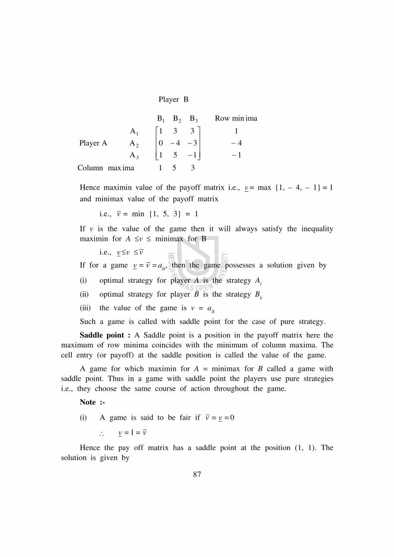
87

Player B

B B B Row ima

Player A

A

A

A

Column ima

1 2 3

1

2

3

1 3 3

0 4 3

1 5 1

1

4

1

1 5 3

min

max

L

NMMM

O

QPPP

Hence maximin value of the payoff matrix i.e., v = max {1, – 4, – 1} = 1

and minimax value of the payoff matrix

i.e., v = min {1, 5, 3} = 1

If v is the value of the game then it will always satisfy the inequalitymaximin for A v minimax for B

i.e., v v v

If for a game v = v = alk, then the game possesses a solution given by

(i) optimal strategy for player A is the strategy Al

(ii) optimal strategy for player B is the strategy Bk

(iii) the value of the game is v = alk

Such a game is called with saddle point for the case of pure strategy.

Saddle point : A Saddle point is a position in the payoff matrix here themaximum of row minima coincides with the minimum of column maxima. Thecell entry (or payoff) at the saddle position is called the value of the game.

A game for which maximin for A = minimax for B called a game withsaddle point. Thus in a game with saddle point the players use pure strategiesi.e., they choose the same course of action throughout the game.

Note :-

(i) A game is said to be fair if v = v = 0

v = 1 = v

Hence the pay off matrix has a saddle point at the position (1, 1). Thesolution is given by

88

(i) the optimal strategy for player A is A1.

(ii) the optimal strategy for player B is B1.

(iii) the value of the game is 1.

Example 3 : For what value of , the game with the following pay offmatrix is strictly determinable?

Player B

B B B

Player A

A

A

A

1 2 3

1

2

3

6 2

1 7

2 4

L

NMMM

O

QPPP

Solution : Ignoring the value of , we shall the maximin and minimax values ofthe pay off. For this purpose, we have

Player B

B B B Row ima

Player A

A

A

A

Column ima

1 2 3

1

2

3

6 2

1 7

2 4

2

7

2

2 1

1 6 2

min

,

max

L

NMMM

O

QPPP

v v

The game is strictly determinable if v = v = v 0

Hence – 1

5.4 Games with mixed Strategy

In some cases, a game can not be solved with pure strategy i.e., for sucha game, no saddle point exists in the case of pure strategy.

In all such cases to solve games, both the players must determine an optimalmixture of strategies to find a saddle point. The optimal strategy mixture for each

89

player may be determined by assigning to each strategy its probability of beingchosen. The strategies so determined are called mixed strategies because they areprobabilistic combination of available choices of strategy.

The value of the game obtained by the use of mixed strategies represents thebest payoff in which player A can expect to gain and the least in which playerB can loose. The expected pay off to a player in a game with arbitrary pay offmatrix A = [a

ij] of m × n is defined as

E(p, q) = i

m

j

n

i ij jp a q

1 1

= pTAq (in matrix notation)

where p = (p1, p

2, ..., p

m) and q = (q

1, q

2, ..., q

n) denotes the mixed strategies

for players A and B respectively.

Also p1 + p

2 + ........ + p

m = 1 and q

1 + q

2 + ....... + q

n = 1, p

i 0, a

j 0,

i = 1, 2, ..., m, j = 1, 2, ..., n.

In particular, if player B takes his pure j-th move or j-th pure strategy thenthe expected gain of A is given by

Ej(p) =

i

m

ij ia p j n

11 2, , ,

Similarly, for particular i-th pure move of player A only, the expected lossof B is given by

Ei(q) =

j

n

ij ja a i m

11 2, , ,

A mixed strategic game or game without saddle point can be solved bydifferent solution methods such as

(i) Algebraic method

(ii) Analytical or calculus method

(iii) Graphical method

(iv) Matrix method

(v) L.P.P. method

(vi) Interactive method.

90

5.5 Minimax and Saddle point PropertiesLet us consider a two person zero sum game with p and q as the set of

strategies for player A and player B respectively. If a player A chooses a strategypp and player B chooses a strategy qQ, then E(p, q) represents the expectedpayoff to player A and – E(p, q) is the expected pay off to player B.

If po be the mixed strategy (announced earlier) of player A, then player Bwill select his best mixed strategy qo to minimize the losses so that

E p q E p qo oq Q

o o( , ) ( , )min

where q Qo o

p q q QE p q E p q v min max min( , ) ( , )

where v represents the maximin value of the game i.e., by selecting po the leastthat A can expect to gain is v .

Similarly, if the player B announced in advance a mixed strategy qo thenobviously player A will select his best strategy po to maximize gain so that

E p q E p q E p q vo op p

o oq Q p p( , ) ( , ) ( , )max min max

where v represents the minimax value of the game i.e., by selecting qo the mostthe B can expect to loose is v . Regarding this, we shall prove the followingtheorem.

Theorem : Let E(p, q) be such that both q Q p p E p q min max ( , ) and q q q Q E p q

max min ( , )

exist, then

minq Q

maxp P E(p, q) max

p P minq Q E(p, q)

Proof : Let po and qo be two arbitrarily chosen mixed strategy for the player A andB respectively.

Then, for every pp, we have

maxp P E(p, qo) E(po, qo)

and for every qQ, we have

minq Q E(po, q) E(po, qo)

91

Hence, from (1 and (2), the inequality

minq Q E(po, q) max

p P E(p, qo)

or, maxp P E(p, qo) min

q Q E(po, q)

holds for all p and q.

Since qo is arbitrarily chosen mixed strategy, hence the above inequality holds for allvalues of q. Hence, if qo be such a strategy for which max

p E(p, q) has the maximum value,the inequality remains true. Therefore,

maxp E(p, q) E(po, q)

Again, since po is any strategy, the above inequality holds even if we select po

which gives the maximum value of E(p, q).

Therefore, max E(p, q) maxp min

q E(p, q)

This proves the theorem.

5.6 Saddle point of a Function

Let E(p, q) be a function of two variables (vectors) p and q in Em and En

respectively. The point (po, qo), poEm, qoEn is said to be the saddle point of thefunction E(p, q) if

E(p, qo) E(po, qo) E(po, q).

Now we shall discuss a theorem regarding the existence of the saddle point of afunction.

Theorem : Let E(p, q) be a function of two variables pEm and qEn, such thatmax

p minq E(p, q) and min

qmax

p E(p, q) exist. Then the necessary and sufficient conditionfor the existence of a saddle point (po, qo) of-E(p, q) is that

E(po, qo) = maxp min

q E(p, q) = minq

maxp E(p, q)

Proof : The condition is necessary i.e., the point (po, qo) is the saddle point of

E(p, q).

92

Hence from the definition of saddle point, we have

E(p, qo) E(po, qo) E(po, q) ......... (1)

for all pEm and pEn.

From (1), clearly, maxp E(p, qo) E(po, qo) holds for all pEm

Hence, minq

maxp E(p, q) E(po, qo) ......... (2)

Similarly, from (1), we have

E(po, qo) minq E(po, q)

i.e., E(po, qo) maxp min

q E(po, q) ......... (3)


minq

maxp E(p, q) max

p minq E(p, q) ......... (4)

But, we know that

minq

maxp E(p, q) max

p minq E(p, q) ......... (5)

Hence from (4) and (5), we have

E(po, qo) = maxp min

q E(p, q) minq

maxp E(p, q)

The condition is sufficient.

Let the point (po, qo) be such that

maxp min

q E(p, q) = minq

maxp E(p, q) ........ (6)

Also, let maxp min

q E(p, q) = minq E(p, q)

and minq max

p E(p, q) = maxp E(p, q0)

Hence from (6), we have

minq E(p0, q) = max

p E(p, qo) ....... (7)

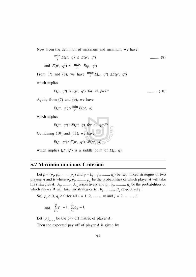
93

Now from the definition of maximum and minimum, we have

minq E(po, q) E(po, qo) ......... (8)

and E(po, qo) maxp E(p, qo)

From (7) and (8), we have maxp E(p, qo) E(po, qo)

which implies

E(p, qo) E(po, qo) for all pEm .......... (10)

Again, from (7) and (9), we have

E(po, qo) minq E(po, q)

which implies

E(po, qo) E(po, q) for all qEn

Combining (10) and (11), we have

E(p, qo) E(po, qo) E(po, q)

which implies (po, qo) is a saddle point of E(p, q).

5.7 Maximin-minimax Criterian

Let p = (p1, p

2, ......., p

m) and q = (q

1, q

2, ......., q

n) be two mixed strategies of two

players A and B where p1, p

2, ........, p

m be the probabilities of which player A will take

his strategies A1, A

2, ........, A

m respectively and q

1, q

2, ........., q

n be the probabilities of

which player B will take his strategies B1, B

2, ........, B

n respectively.

So, pi 0, q

j 0 for all i = 1, 2, ......., m and j = 2, ........, n

and p qii

m

jj

n

1 11 1, .

Let [aij]

m × n be the pay off matrix of player A.

Then the expected pay off of player A is given by

94

E p q p a qi ij jj

n

i

m( , )

11

Now, if maximin-minimax criterian for a mixed strategy game is applied to

E(p, q), then we have for player A, v = maxp min

q E(p, q)

RSTUVW

LNM

OQP

max minp j

i iji

mp a

1

RSTUVW

LNM

OQP

max min , ,....... ,p

i ij i i i ini

m

i

m

i

mp a p a p a2

111

Here minj

i iji

mp a

RST

UVW1denotes the least expected gain to player A if the player B uses

his j-th strategy i.e., Bj. For player B,

v a qq i

ij jj

m

RSTUVW

LNM

OQP

min max1

denotes the expected loss to player B if the player AA

uses his i-th strategy i.e., Ai.

Now, in general, however, when pi and qj correspond to the optimal strategy then theequality sign holds and in that case i.e., when v = v , then the pair of strategies (p, q)

is called a saddle point of E(p, q).

The above result is called maximin-minimax property.

Theorem : For any two person zero sum game when the optimal strategiesare not pure (without saddle point) for which the pay off matrix for player A is

Player B

B B

A

Player A A

1 2

1

2

11 12

21 22

a a

a a

LNM

OQP

The optimal mixed strategies (p1, p

2) of A and (q

1, q

2) of B are determined

95

p

p

a a

a a

q

q

a a

a a1

2

22 21

11 12

1

2

22 12

11 21

;

where p1 + p

2 = 1, q

1 + q

2 = 1 and the value of game is given by

va a a a

a a a a

11 22 12 21

11 22 12 21( )

Proof : Since (p1, p

2) and (q

1, q

2) are the mixed strategies for players A and

B respectively.

Then, p1 + p

2 = 1, q

1 + q

2 = 1, p

1, p

2 0 and q

1, q

2 0

Now the expected gain of player A can be calculated as follows :

E1(p) = a

11p

1 + a

21p

2 when player B uses strategy B

1 and

E2(p) = a

12p

2 + a

22p

2 when player B uses strategy B

2

Similarly, the expected loss of player B can be computed as follows :

E1(q) = a

11q

1 + a

12q

2 if player A uses strategy A

1 and

E2(q) = a

21q

1 + a

22q

2 if player A uses strategy A

2

If v be the value of the game, then player A expects a least possible gain v.

Then, E1(p) v

and E2(p) v

Again, as the maximum possible loss of player B is v, then

E1(q) v and E

2(q) v

Now, considering the above inequalities as strict equalities, we have

E1(p) = v, E

2(p) = v and E

1(q) = v, E

2(q) = v

i.e., a11

p1 + a

21p

2 = v ........ (1)

a12

p1 + a

22p

2 = v ........ (2)

and a11

q1 + a

12q

2 = v ........ (3)

a21

q1 + a

22q

2 = v ........ (4)


a11

p1 + a

21p

2 = a

12p

1 + a

22p

2

or, (a11

– a12

)p1 = (a

22 – a

21)p

2

96

or,p

p

a a

a a1

2

22 21

11 12

Now, p2

= p

p pp p2

1 21 2 1

[ ]

=

1

1

1

11

2

22 21

11 12

11 12

11 22 12 21p

p

a a

a a

a a

a a a a

( ) ( )

p pa a

a a a a1 222 12

11 22 12 21

1

( ) ( )

Then the value of the game is given by

v = E1(p) = a11p1 + a21p2

= a a a a

a a a a11 22 12 21

11 22 12 21

( ) ( )

Again, from (3) and (4), we have

a11q1 + a12q2 = a21q1 + a22q2

or, (a11 – a21)q1 = (a22 – a12)q2

or,q

q

a a

a a1

2

22 12

11 21

This proves the theorem.

This method (described in the above theorem) for finding the values p1,p2,q1,q2 and thevalue of the game is known as the algebraic method. By this method, it is not possible to solveeasily any game without sadle point whose pay off matrix is of m × n order (m, n > 2).

5.8 The rules of DominanceSometimes, in a rectangular game, it is seen that one or more pure strategy

(or strategies) of a player are inferior to at least one of the remaining strategies.In such cases, this inferior strategy is never used. In other words, we can saythat this inferior pure strategy is dominated by a superior pure strategy. In suchcases of dominance, we can reduce the size of pay off matrix by removing the

97

pure strategies which are dominated by other strategies. Hence the rules ofdominance are used to reduce the size of the payoff matrix. This rules are speciallyused for solving two person zero sum game without saddle point.

Rule 1 : If each element in a row (say i-th row i.e., Ri) of a pay off matrix

is either less than or equal to the corresponding element in another row, say j-th row i.e., R

j, then the i-th strategy is dominated by j-th strategy and can be

deleted that row (i.e., i-th row) from the pay off matrix.

In other words, player A will never use that strategy because if player Achooses such strategy then he will gain less payoff.

Rule 2 : If each element in a column, say i-th column i.e., Ci of a payoff

matrix is either greater than or equal to the corresponding element in anothercolumn, say j-th column i.e., C

j, then the i-th strategy is dominanted by j-th

strategy and can be deleted that column i.e., i-th column from the payoff matrix.

Rule 3 : A strategy k can also be dominated if it is inferior to a convexcombination of several other strategies. In this case, a row or column correspondingthis strategy can be deleted. This domination will be decided as per rules 1 and2 stated earlier.

Rule 3 is called the modified dominance property. It is pointed out that theelement or probability value corresponding to the deleted strategy by the rules ofdominance is taken as zero.

Example 4 : Solve the game whose payoff matrix is given by

Player B

Solution : First of all, we shall find out the maximin and minimax value incase of pure strategy.

Player A

98

B B B B Row ima

A

A

A

A

column ima

1 2 3 4

1

2

3

4

1 2 2 2

3 1 2 3

1 3 2 1

2 2 0 3

2

1

1

3

3 3 2 3

min

max

L

N

MMMM

O

Q

PPPP

In case of pure strategy, maximin value = 1 and minimax value = 2. Asmaximin value minimax value, this game has no saddle point in case of purestrategy. Hence this game can be solved for the mixed strategy. For this purpose,we shall try to reduce the size of the payoff matrix by using the dominance rule.

Since every element of fourth row is less than the corresponding elements ofthird row, therefore from player A’s point of view, fourth strategy i.e., A

4 is

dominated by 3rd strategy i.e., A3 and hence we can delete the fourth row. In

this situation, the optimal strategy will not be affected. Now deleting 4-th row,we get the reduced payoff matrix as follows :

B B B B

A

A

A

1 2 3 4

1

2

3

1 2 2 2

3 1 2 3

1 3 2 1

L

NMMM

O

QPPP

Again, from player B’s point of view, 4-th strategy i.e., B4 is dominated by

B1 as every element of 4-th column is either greater or equal to the corresponding

element of 1-st column. Then by deleting the 4-th column, we get the reducedpayoff matrix as follows :

B B B

A

A

A

1 2 3

1

2

3

1 2 1

3 1 2

1 3 3

L

NMMM

O

QPPP

From the reduced payoff matrix, it is seen that none of the pure strategiesof players A and B is inferior to any of their other strategies. However, the

99

covex combination due to strategies A2 and A

3 (i.e., the average of 2nd & 3rd

row i.e., 1, 2, 2) is superior than the payoff due to the strategy A1. Thus strategy

A1 may be deleted and we get the reduced payoff matrix as follows :

B B B

A

A

1 2 3

2

3

3 1 2

1 3 2LNM

OQP

In this reduced matrix, the convex combination due to strategies B1 and B

2

is superior than the payoff due to strategy B2. Thus, strategy B

3 may be deleted

and we get the reduced 2 × 2 pay off matrix as follows :

B B

A

A

1 2

2

3

3 1

1 3LNM

OQP

Now, we have to solve this reduced game whose payoff matrix is of 2 × 2order. Clearly, this game has no saddle point and can not be reduced further.Therefore, the optimal strategies will be mixed strategies.

Let the player A chooses his strategies A2 and A

3 with probabilies p

2 and p

3

and that of B is q1 and q

2.

p2 + p

3 = 1, q

1 + q

2 = 1 and p

2, p

3, q

1, q

2 > 0 and v be the value

of the game.

To determine the optimal values of p1 and p

2, we have

3p2 – p

3 = p

2 + 3p

3 = v

which implies p p p2 1 223

113

To determine the optimal values of q1 and q

2, we have

3q1 + q

2 = – q

1 + 3q

2

which implies q q1 213

23

The value of the game v p p 3 323

13

532 3 .

100

Hence the solution of the game is as follows :

Optimal strategies are p q* , , , , * , , , 0 23

13 0 1

323 0 0e j e j and the value of the

game is 53 .

5.9 Graphical Solution of 2 × n or m × 2 games

Any rectangular game of order 2 × n or m × 2 can be reduced to a 2 × 2game by using graphical method and then the reduced game of order 2 × 2 canbe solved by algebraic method.

Let us consider a 2 × n game without saddle point. Its payoff matrix is asfollows :

Player B

B B B

A

Player A A

n

n

n

1 2

1

2

11 12 1

21 22 2

...........

...........

...........

a a aa a a

LNM

OQP

Let p = (p1, p

2) and q = (q

1, q

2, ........., q

n,) be the mixed strategies for

players A and B respectively. When player B uses his pure strategy Bj, then the

expected gain of player A is given by

Ej(p) = a

ijp

1 + a

2 j p

2 = a

1jp

1 + a

2j(1 – p

1), j = 1, 2, ........, n(1) as p

1 + p

2 = 1

Clearly, both p1 and p

2 must lie in the open interval (0, 1) [because if either

p1 = or p

2 = 1, the game reduces to a game of pure strategy which is against

our assumption]. Hence Ej(p) is a linear function of either p

1 or p

2. Considering

Ej(p) as linear function of p

1 (say), we have

Ej(p) = a

2j for p

1 = 0

= a1j for p

1 = 1

Hence Ej(p) represents a line segment joining the points (0, a

2j) and (1, a

1j).

Now player A expects a least possible gain v. Therefore, Ej(p) v for all j.

Now considering the strict equations for inequalities and with the help of graphical

101

method, we shall find out two particular moves or choices of B which willmaximize the minimum gain of A.

Let us draw two parallel lines p1 = 0 and p

1 = 1 at unit distance apart. Now

draw n line segments joining the points (0, a2j) and (1, a

1j), j = 1, 2, ..., n. The

lower envelope (or lower boundary) of these line segments (indicate it by thickline segment) will give the minimum expected gain of A as a function of p

1.

Now the highest point of lower envelope will give the maximum of minimumgain of A. The line segments passing through the point corresponding to B’s twopure moves, say, B

k and B

l are the critical moves for B which will maximize the

minimum expected gain of A. Now the 2 × 2 payoff matrix corresponding to A’smoves A

1, A

2 and B’s moves B

k, B

l will produce the required result. Thus solving

the 2 × 2 game algebraically, we can find the value of the game.

If there are more than two line segments passing through the highest (maximin)point there are ties for the optimum mixed strategies for the player B. Thus anytwo such lines with opposite sign slopes will determine an alternative optimumfor B.

Again, if there are more than one maximin point, alternative optimum existcorresponding to these points.

Example 5 : Solve the following 2 × 4 game graphically :

Player B

Player A

Solution : Clearly, the given problemdoes not possess any saddle point in caseof pure strategy. Hence this problem canbe solved with mixed strategy.

Let the player A play with mixedstrategy p = (p

1, p

2) where p

1 + p

2 = 1 and

both p1 and p

2 lie in the open interval

(0, 1).

Fig. : 5.1

B1 B2 B3 B4

A1 1 3 -3 7

A2 2 5 4 -6[ ]

102

Then player A’s expected gains against B’s pure moves are given be

B’s pure move A’s expected gain E(p1)

B1

E1(p

1) = p

1 + 2p

2 = p

1 + 2(1 – p

1)

B2

E2(p

1) = 3p

1 + 5(1 – p

1)

B3

E3(p

1) = – 3p

1 + 4(1 – p

1)

B4

E4(p

1) = 7p

1 – 6(1 – p

1)

draw two vertical lines p1 = 0 and p

1 = 1 at unit distance apart. Make the lines

p1 = 0 and p

1 = 1 by using the same scale as given in the figure. Now draw

the line segments for the expected gain equations between two vertical lines p1 =

0 and p1 = 1. These line segments represent A’s expected gain due to B’s pure

move. We denote these line segments as B1, B

2, B

3, B

4. Since the player A

wishes to maximize his minimum expected gain. The highest point of intersectionH of two line segments B

3 and B

4 represents the maxinin expected value of the

game for player A. Hence the solution to the original game reduces to that of thesimpler game with 2 × 2 payoff matrix given below.

Player B

Player A

B B

A

A

3 4

1

2

3 7

4 6

LNM

OQP

Now, if p = (p1, p

2) and q = (q

3, q

4) be the optimum strategies for players A

and B, then we have

pa a

a a a a122 21

11 22 12 21

6 43 6 7 4

1020

12

( ) ( ) ( )

p p2 1112

Again, q q q3 4 36 7

3 6 7 41320

1720

( ),

and the value of the game is given by

va a a a

a a a a

11 22 12 21

11 22 12 21

18 2820

12( ) ( )

103

Hence the solution of the game is as follows :

(i) Optimal strategies p q* , * , ,, , 12

12

1320

7200 0d i d i

(ii) the value of the game = 12

Example 6 : By graphical method, solve the game whose payoff matrix isgiven below.

Player B

Player A

B B B B

A

A

1 2 3 4

1

2

2 2 3 1

4 3 2 6

LNM

OQP

Solution : In a similar way, draw thegraph. Here three lines pass at the highestpoint of the lower envelope. Thus,accordingly, we get 3C

2 i.e. 3 square matrics

of order 2 and three optimal solutions. Butactually we shall have to select such pair oflines which have the slope opposite in sign.Thus, we get two reduced game with payoffmatrix of order 2 × 2 as follows :

Fig. : 5.2

Player B Player B

Player A

B B

A

A

2 3

1

2

2 3

3 2

LNM

OQP

and Player A

B B

A

A

3 4

1

2

3 1

2 6

LNM

OQP

Solving these, we get the value of the game as 52 and the optimal strategies as

p q* , , * , , , 12

12

12

120 0d i d i for first case and

p q* , , * , , , 12

12

78

180 0d i d i for 2nd case.

Any m × 2 game problem can be solved by using B’s mixed strategy q = (q1, q

2)

where q1+ q

2 = 1 and both lie in the open interval (0, 1), and A’s particular critical

104

moves can be determined graphically. In this case, the problem is to determine theminimum of the maximum expected loss of B. Thus we shall have to select thelowest point (minimax) of upper envelope and A’s critical moves are the moves linesegments corresponding to which pass through the minimax point. Now selecting a2 × 2 payoff matrix, the value of the game can be determined easily.

Example 7 : solve the game whose payoff matrix is as follows :

Player B

Player A

B B

A

A

A

1 2

1

2

3

2 3

2 5

0 1

L

NMMM

O

QPPP

Here H be the lowest point of the upperenvelope. As the point H be the point ofintersection of two line segments A

1, A

2, the

payoff matrix of the reduced game will be

Now solving the reduced game by algebraic method, easilywe shall find the optimal strategies and the value of the game.

For this problem, optimal strategies will be p * , , ,712

512 0d i

p * ,23

13d i and the value of the game is 1

3 .

5.10 Summary

In this unit, two person zero sum games and its solution procedure havebeen discussed. Particularly, the solution procedure of games with pure strategyhave been discussed by maximin-minimax criteria whereas Games with mixedstrategies by two wellknown methods viz. Algebraic method and graphical method.Also, to reduce the size of the payoff matrix of a game, the dominance andmodified dominance properties have been discussed. To illustrate the differentmethods for solving the games with/without saddle point, some examples havebeen presented.

B B

A

A

1 2

1

2

2 3

2 5

LNM

OQP

Fig. : 5.3

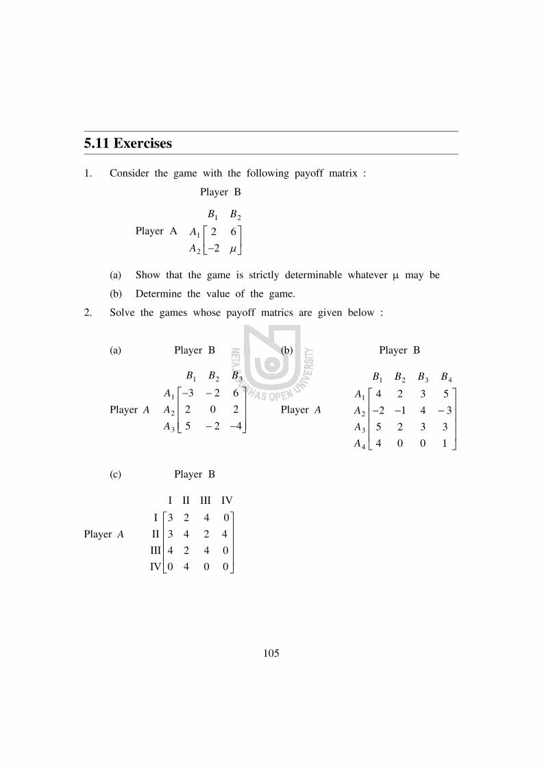
105

5.11 Exercises

1. Consider the game with the following payoff matrix :

Player B

Player A

B B

A

A

1 2

1

2

2 6

2LNM

OQP

(a) Show that the game is strictly determinable whatever may be

(b) Determine the value of the game.

2. Solve the games whose payoff matrics are given below :

(a) Player B (b) Player B

Player A

B B B

A

A

A

1 2 3

1

2

3

3 2 6

2 0 2

5 2 4

L

NMMM

O

QPPP

Player A

B B B B

A

A

A

A

1 2 3 4

1

2

3

4

4 2 3 5

2 1 4 3

5 2 3 3

4 0 0 1

L

N

MMMM

O

Q

PPPP

(c) Player B

Player A

I II III IV

I

II

III

IV

3 2 4 0

3 4 2 4

4 2 4 0

0 4 0 0

L

N

MMMM

O

Q

PPPP

106

3. Solve the following 2 × 2 games using mixed strategies :

(a) Player B (b) Player B

Plyer A

B B

A

A

1 2

1

2

6 4

1 2

LNM

OQP

Player A

B B

A

A

1 2

1

2

4 2

1 5

LNM

OQP

4. Use graphical method in solving the following games

(a) Player B

Player A

B B B B

A

A

1 2 3 4

1

2

1 2 3 7

2 5 4 6

LNM

OQP

(b) Player B

Player A

5.12 References

1. P. M. Karak, Linear Programming and Theory of Games, New CentralBook Agency (P) Ltd.

2. H. A. Taha, Operations Research, An Introduction, PHI, India.

3. Swarup, Gupta and Mohan, Operations Research, Sultan Chand & Sons,India.

4. D. Sharma, Operations Research, Kedar Nath Ram Nath & Co. India.

107

Unit 6 p Project Management PERT and CPM

Structure

6.0 Objectives

6.1 Introduction

6.2 Advantages of Networking Analysis

6.3 Basic Camponents

6.4 Common Errors

6.5 Rules of Network Construction

6.6 Numbering the Events

6.7 Critical Path Analysis

6.7.1 Forward Pass calculations method

6.7.2 Backward Pass calculations method

6.7.3 Determination of Floats and slack times

6.8 PERT Analysis

6.9 Probability of meeting the schedule time

6.10 Difference between PERT and CPM

6.11 Project times cost trade off

6.12 Summary

6.13 Exercises

6.14 References

6.0 Obectives

Project is a set of activities which are related to each other and to becompleted to signal the end of the given project. Project management is differentform manufacture, sales and marketing and yet, it involves every one of them.

108

Setting up a factory is a project, so also building a bridge or developing technologyfor a new telephone network in a township. This involves activities likescheduling, sequencing and forecasting. This also calls for managerial functionslike planning, organising, coordinating, directing and staffing. This also involvestransformation of resources into goods and services. Project management is a onetime task. It is an organising and structuring concept to obtain optimum utilizationof resources employeed. It is the manifestatin of systems concept in management.

In this unit, we shall discuss the main objectives of the project management,with its different terminologies. Hence also we shall present two popular andpowerful techniques used in network of a project. These are (i) PERT(Programme Evaluation and Review Technique) and (ii) CPM (Critical PathMethod). In these techniques, only the duration of the activities of a project willbe considered. Finally, we shall discuss the time-cost trade off and its algorithmincluding the cost aspects in the project scheduling.

6.1 Introduction

A project is a well defined set of jobs, tasks or activities, all of which mustbe competed to finish the project. Construction of a highway, power plant,production and marketing of a new product, research and development work arethe examples of project. Such projects involve large number of inter-relatedactivities (or tasks) which must be completed in a specified time, in a specifiedsequence (or order) and require resources such as personnel, money, materials,facilities and/or space. The main objective before starting any project is to schedulethe required activities in an efficient manner so as to

(i) complete it on or before a specified time limit

(ii) minimize the total time

(iii) minimize the time for a prescribed cost

(iv) minimize the cost for a specified time

(v) minimize the total cost

(vi) minimize the idle resources.

109

Therefore, before starting any project, it is very much essential to prepare aplan for scheduling and controling the vairous activities involved in the project.The techniques of O.R. used for planning, scheduling and controling large andcomplex projects are very often referred to as network analysis, network planningfor network scheduling techniques. IN all these techniques, a project is brokendown into various activities whcih are arranged in logical sequence in the form ofnetwork. This approach assists managers to visualize a project a s a numnber oftasks which can be easily defined in terms of its duration, cost, starting time. Thesequence of activities are also defined. There are two basic planning and controltechniques that utilize a network to complete a predetermined project or schedule.There are PERT (Program Evaluation and Review Technique) and CPM (CriticalPath Method). PERT network was developed in 19546-58 by a research team ofUS Navy’s Polaris Nuclear Submarine Missile development project. Since 1958,this technique has been used to plan in all most all types of projects. At the sametime but independently, CPM was developed jointly by two companies : E. I.Dupont Comnany and Remington Rand Corporation. Other network techniqueswere PET (Performance Evaluation Programme), LCES (Least Cost Estimating andScheduling), SCANS (Scheduling and Control by automated Network System).

The work involved in a project can be dividee into three phases correspondingto the management functions of planning, scheduling and control.

Planning : This phase involves setting the objectives of the project and theassumptions to be made. Also it involves the listing of tasks or jobs that must beperformed to complete a project under consideration. In this phase, men, machinesand materials requred for the project in addition to the estimates of costs andduration of the various activities of the project are also determined.

Scheduling : This consists of laying the activities according to the precedenceorder and determining.

(i) the starting and finishing times for each activity

(ii) the ciritical path on which the activities requre special attention and

(iii) the slack and float for the non ciritcal paths.

Controlling : This phase is exercised after planning and scheduling whichinvolves the following :

110

(i) Making periodical progress reports

(ii) Revieuing the progress

(iii) Analysing the status of the project

(iv) Management decisios regarding updating, crashing and resourceallocation,etc.

6.2 Advantages of Network Analysis

(i) It shows interrelationships of all jobs in the project.

(ii) It gives a clear picture of relationship controlling the order of performanceof various activities than a typical bar chart.

(iii) It helps in communication of ideas. The pictorial approach helps to clarifythe verbal instructions.

(iv) It provides time schedule containing much more information than othermethods like Barcharts etc.

(v) It identifies jobs which are critical for a project completion data.

(vi) It permits an accure forecast of resource requirement.

(vii) It provides a method of resource allocation to meet the limiting conditionand to maintain or to minimize the overall costs.

(viii)It integrates all elements of a program to whatever detail is desired by themanagement.

(ix) It relates time to costs which allows a rupee value to be placed on proposedchanges.

6.3 Basic Components

There are two basic components in network. These are

(i) Event/ Node (ii) Activity

111

Event/Node : A node/event is a particular instant in time showing the end orbeginning of one or more activities. It is a point of accomplishment or decision.The starting and end points of an activitiy are thus described by two events usuallyknown as the tail event and head event respectively. An event is generallyrepresented by a circle, rectangle, hexagon or some other geometric shapes. Thesegeometric shapes ae numbered for distinguishing an activity from antoher one. Theoccurance of an event indicates that the work has been accomplished upto thatpoint.

Merge and burst events : It is necessary for an event to be the ending eventof only one activity but can be the ending event of two or more activities. Suchevent is defined as merge event.

If the event happens to be the beginning event of two or more activities it isdefined as a burst event.

Activity : An activity is a task or item of work to be done that consumestime, effort, money or other resources. Activities are represented by arrows.

Activities are identified by the numbers of their starting (tail) event and ending(head) event. Generally, an ordered pair (i, j) represents an activity where andevents i and j represent the starting and ending of the activity respectively. Activitiesare also denoted by capital alphabets.

activity

Fig. 6.1tail event/node head event/node

Merge event burst event

Fig. 6.2(a) Fig. 6.2(b)

activity

startign event

(tail event)ending (head) event

112

The activities can be further classified into different categories;

(i) Predecessor activity : An activity which must be completed before oneor more other activities stsart is known as predecessor activity.

(ii) Successor activity : An activity which started immediately after one ormore of other activities are completed is known as successor activity.

(iii) Dummy activity : In connecting events by activities showing their interdependencies, very often a situation arises where a certain event j can not occuruntil another event i has taken place but, the activity connecting i and j does notinvolve any time or expenditure of toehr resources. In such a case, the activityis called the dummy activity. It is depicted by dotted line in the network diagram.

Let us consider the example of a car taken to a garage for cleaning. Insideas well as outside of the car is to be cleaned before it is taken away from thegarage. The events can be put doen as follows :

Event 1 : Start the car from house

2 : Park the car in garage

3 : Compete outside cleaning

4 : Compete inside cleaning

5 : Take car from garage

6 : Park the car in house

It is assumed that inside cleaning and outside cleaning can be done concurrentlyby two assistants of the garage. Activities B and C represent these cleaning

Fig. 6.4

113

operations. What do activities D and E stand for? Their time consumpotions arezero but ehey express the condition that events 3 and 4 must occur before theevent 5 can take place. Activities D and E are called the dummy activities.

Network : It is the graphic representation of logically and sequentiallyconnected arrows and nodes representing activities and events of a project. Networksare also called arrow diagram.

Path : An unbroken chain of activity arrows connecting the initial event tosome other event is called a path.

6.4 Common Errors

There are three common errors in a network construction.

Looping (cycling) : In a network diagram looping error is also known ascycling error. Drawing an endless loop in a network is knwon as error of looping.A looping network is given below.

It should be avoided in construction of a network.

Dangling : To disconnect an activity before the completion of all the activitiesin a network diagram is known as dangling. It should be avoided.

Fig. 6.5

Fig. 6.6

114

In that case, a dummy activity is introduced in order to maintain the continuityof the system.

Redundancy : If a dummy activity is the only activity emanating from anevent and which can be eliminated is known as redundancy.

6.5 Rules of Network Construction

For the construction of a network, generally, the following rules are followed:

(i) Each activity is represented by one and only one arrow.

(ii) Crossing an arrow and curved arrows should be avoided, only straightarrows are to be used.

(iii) Each activity must be identified by its starting and ending node.

(iv) No event can occur until every activity preceeding it has been completed.

(v) An event can not occur twice i.e. there must be no loops.

(vi) An activity succeeding an event can not be started until that event hasoccured.

(vii) Events are numbered to identity an activity uniquely. The number oftail event (starting event) should be lower than that of the head (ending)event of an activity.

(viii) Between any pair of nodes (events), there should be one an only oneactivity. However, more than one activity may emanate from a node orterminate to a node.

Fig. 6.7

115

(ix) Dummy activities should be introduced if it extremely necessary.

(x) The network has only one entry point called the starting event and one pointof emergence called the end or terminal event.

6.6 Numbering the Events

After the network is drawn in a logical sequence every event is assigned anumber. The number sequence must be such so as to reflect the flow of thenetwork. In numbering the events, Fulkerson’s (D. R. Fulkerson) rules are used.These rules are as folows :

(i) Event number should be unique.

(ii) Event numbering should be carried out on a sequential basis from leftto right.

(iii) An initial event is one which has all outgoing arrows with no incomingarrow. In any network, there will be one such event. Nukmber it 1.

(iv) Delete all arrows emerging from event – 1. This will crete atleast onemore initial event.

(v) Number these intial events as 2, 3, ..., etc.

(vi) Delete all emerging arrows from these numbered events which will createnew initial events.

(vii) Repeat step-(v) & (vi) until the last event is obtained which has noarrow emerging from it. Number the last event.

Esmaple 1 : Construct a network of each of the projects whose activitiesand their precedence relationships are given below. Then numebr the events.

Activity A B C D E F G H I

Immediate — A A — D B, C, E F D G, HPredecasser

116

6.7 Critical Path Analysis

Once the network of a project is constructed, the time analysis of the networkbecomes essential for planning various activities of the project. The main objectiveof the time analysis is to prepare a planning schedule of the project. The planningschedule should include the following factors :

(i) Total completion time for the prohject.

(ii) Earliest time when each activity can start.

(iii) Latest time when each activity can be started without delaying the totalproject.

(iv) Float for each activity i.e. the duration of time by which the completionof an activity can be delayed without delaying the total project completion.

(v) Identification of critical activities and critical path.

Notations : The following notations are used in this analysis.

Ei = Earliest occurance time of event i i.e., it is the earliest time at which

the event i can occur without affecting the total project duration.

Li

= Latest allowable occurance time of event i. It is the latest allowabletime at which an event can occur without affecting the total projectduration.

tij

= Duration of activity (i, j)

ESij

= Earliest starting time of activity (i, j)

Fig. 6.8

117

LSij

= Latest starting time of activity (i, j)

EFij

= Earliest finishing time of activity (i, j)

LFij

= Latest finishing time of activity (i, j)

The critical path calculations are done in the following two ways :

(a) Forward Pass Calculations method

(b) Backward Pass Calculations method

6.7.1 Forward Pass Calculations Method

In this method, calculations begin from the initial event, proceed through theevents in an increasing order of event number and end at the final event of thenetwork. At each node (event), the earliest starting and finishing times arecalculated for each activity. The method may be summarized as follows :

Step 1 : Set Ej = 0, i = 1

Step 2 : Calculate the earliest starting time ESij for each activity that

begins at event i i.e. ESij = E

i for all activities (i, j) that start

at node i.

Step 3 : Calculate the earliest finishing time EFij of each activity that begins

at event i by adding the earliest starting time of the activity withthe duration of the activity thus EF

ij = ES

ij + t

ij = E

i + t

ij

Step 4 : Go to next event (node), say event j(j > i) and compute theearliest occurance time for event j. This is the maximum of theearliest finishing times of all activities ending into that event i.e.,

Ej = ? ? ? ?ij i ij

i iMax EF Max E t? ? for all immediate predecessor

activities.

Step 5 : If i = n (final event number), then the earliest finishing time forthe project is given by

En = ? ? ? ?ij i iji i

Max EF Max E t? ? for all terminal activites.

6.7.2 Backward Pass Calculations Method

In this method, calculations begin from the terminal event, proceed throughthe events in a decreasing order of event numbers and end at the initial event

118

of the network. All each node (event), the latest starting and finishing times arecalculated for each activity. The method may be summarized as follows :

Step 1 : Set En = 0, j = n

Step 2 : Calculate the latest finishng time LFij for each activity that ends at event

j i.e, LFij = L

j for all activities (i, j) that end at node j.

Step 3 : Calculate the latest starting time LSij of each activity that ens at event

j by sutracting the duration of each activity from the latest finishing timefo the activity. Thus

LSij = LF

ij – t

ij = L

j – t

ij

Step 4 : Proceed backward to the node in the sequence that decrease j by 1.Also compute the latest occurance time of node i (i < j).This is theminimum of the latest starting times of all activities starting from tahtevent i.e.

Lj = min { } min{ }ij j ijj j

LS L t? ? for all immediate successor activities.

Step 5 : If i = 1 (initial node), then

L1 = min { } min{ }ij j ij

j jLS L t? ? for all initial activities.

6.7.3 Determination of Floats and Slack times

When the network diagram is completely draw, properly labelled, earliest andlatest event times are computed, then the next object is to determine the floatsof each activity and slack time of each event.

The float of an activity is the amount of time by which it is possible to delayits completion time without affecting the total project completion time. There arethree types of activity floats :

(i) Total float, (ii) Free float, (iii) Independent float

Total float : The float of an activity represnets the amount of time by whichan activity can be delayed without delay in the project completion time.

Mathematically, the total float of an activity (i, j) is the difference betweenthe latest start time and earliest start time of that activity (or the difference betweenthe earliest finish time and latest finish time). Hence the total float for an activity(i, j) is denoted by TF

ij and is computed by the formula.

119

TFij = LS

ij – ES

ij or TF

ij = LF

ij – EF

ij

or TFij = L

j – (E

j + t

ij)

Free float : Sometimes, it may be needed to know how much an activity’scompletion time may be delayed without causing any delay in its immediatesuccessor activities. This amount of float is called free float. Mathematically, thefree flat for an activity (i,j) is denoted by FF

ij and is computed by,

FFij = E

j – E

i – t

ij

As TFij = L

j – E

j – t

ij and L

j E

j

TFij E

j – E

j – t

ij i.e. TF

ij FF

ij

Hence for all activities, free float can take values from zero upto total floatbut it can nto exceed total float.

Again, free float is very useful for rescheduling the activities with minimumdisruption of earlier plans.

Independent float : In some cases, the delay in the completion of an activityneither affects its predecessor nor the successor activities. This amount of delayis called independent float. Mathematically, independent of an activity (i, j) denotedby IF

ij is computed by the formula,

IFij = E

i – L

i – t

ij

The negative independent float is always taken as zero.

Event slack or Event float : The slack of an event is the difference betweenits latest time and its earliest time. Hence for an event i,

slack = Li – E

i

Critical Event : An event is said to be critical if its slack is zero ie., Li =

Ei for i-th event.

Critical activity : An activity is critical if its total float is zero i.e. LSij =

ESij or LF

ij = EF

ij for an activity (i, j).

Otherwise, as activity is called non-critical.

Critical Path : The continuous chain or sequence of critical activities in anetwork diagram is called the ciritcal path. This path is the longest path in thenetwork from starting event to ending event and is shown by a dark line or

120

double lines to make distinction from other non-critical path.

The length of the critical path is the sum of the individual times of all criticalactivities lying on it and define the minimum time required to complete the project.

The ciritical path on a network diagram can be identified as

(i) For all activities (i, j) lying on the critical path the E-values and L-valuesfor tail and head events are equal i.e. E

i = L

j & E

i = L

i

(ii) On the critical path, Ej – E

j = L

j – L

i = t

ij

Main features of the critical path

The critical path has two main features :

(i) If the project has to be shortened, then some of the activities on thatpath must be shortened. The application of additional resources on otheractivities will not give the desired results unless that critical path isshortened first.

(ii) The variation in actual performance from the expected activity durationtime will be completely reflected in one-to-one fashion in the anticipatedcompletion of the whole project.

Example 2 : Determine the critical path, minimum time of completion of theproject whose network diagram is shown below. Find also the different floats.

Solution : Forward pass calculations

At node 1 : Set E1 = 0

At node 2 : E2 = E

1 + t

12 = 0 + 20 = 20

Fig. 6.9

121

At node 3 : E3 = E

1 + t

13 = 0 + 23 = 23

At node 4 : E4 = ? ?4

1,3max i ii

E t?

? = max {E1 + t

14), E

3 + t

34}

= max {0 + 8, 23 + 16} = 39

At node 5 : E5 = ? ?5

2,4max i ii

E t?

? = max {E2 + t

25, E

4 + t

45}

= max {20 + 19, 39 + 0} = 39

At node 6 : E6 = ? ?6

4,5max i ii

E t?

? = max {E4 + t

46, E

5 + t

56}

= max {39 + 18, 39 + 0} = 57

At node 7 : E7 = ? ?7

3,5,6max i ii

E t?

? = max {E3 + t

37, E

5 + t

57, E

6 + t

61}

= max {23 + 24, 39 + 4, 57 + 10} = 67

Backward pass calculations

At node 7 : Set L7 = E

7 = 67

At node 6 : L6 = L

7 – t

67 = 67 – 10 = 57

At node 5 : L5 = ? ?5

6,7min j jj

L t?

? = min (L6 – t

56, t

7 – t

57)

= min {57 – 0, 67 – 4} = 57

At node 4 : L4 = ? ?4

5,6min j jj

L t?

? = min {L5 – t

45, L

6 – t

46}

= min {57 – 0, 57 – 18} = 39

At node 3 : L3 = = min {L

4 – t

34, L

7 – t

37}

= min {39 – 16, 67 – 24} = 23

At node 2 : L2 = L

5 – t

25 = 57 – 19 = 38

At node 1 : L1 = ? ?1

2,3,4min j j

jE t

?? = min {L

2 – t

12, L

3 – t

13, L

4 – t

14}

= min {38 – 20, 23 – 23, 39 – 8} = 0

34,7

min j jj

L t

122

To find the critical activities and different floats, He construct the following table.

Duration Earliest time Latest time Float

Activity of Start finish start finish Critical

activity (Ei) (E

i + t

ij) (L

i + t

ij) (L

i) activity

(1, 2) 20 0 20 18 38 18 0 0

(1,3) 23 0 23 0 23 0 0 0 (1, 3)

(1, 4) 8 0 8 31 39 31 31 31

(2, 5) 19 20 39 38 57 18 0 0

(3, 4) 16 23 39 23 39 0 0 0 (3, 4)

(3, 7) 24 23 47 43 67 20 20 20

(4, 5) 0 39 39 57 57 18 0 0

(4, 6) 18 39 57 39 57 0 0 0 (4, 6)

(5, 6) 0 39 39 57 57 18 18 0

(5, 7) 4 39 43 63 67 24 24 16

(6, 7) 10 57 67 57 67 0 0 0 (6, 7)

Tot

alL j–

Ei

– t ij

Free

Ej–

Ei

– t ij

Inde

pend

dent

Eij

L i – t

ij

From the above table, it is clear that the critical activites (zero total float) are (1,3), (3, 4), (4, 6) and (6, 7). Hence the critical path is 1 – 3 – 4 – 6 – 7 and durationof the project is 67 time units (as E

7 = L

7 = 67).

6.8 PERT Anlysis

Time estimates : It is very difficult to estimate time required for the executionof each activity or job because of various uncertainties. Taking the uncertaintiesinto account, three types of time estimates are generally obtained.

The PERT system is based on these three time estimates of the performancetime of an activity.

(i) Optimistic time (t0) : This is the estimate of the shortest possible time

in which an activity can be completed under ideal conditions.

(ii) Pessimistic time (tp) : This is the maximum time which is required to

123

perform the activity under extremely bad conditions. However suchconditions donot include labour strike or acts of nature (like flood, earthquake, tornedo etc.).

(iii) Most likely time (tm) : This is the estimate of the normal time in which

an activity would take. This time estimate lies between the optimisticand pessimistic time estimates. Statistically, it is the modal value ofduration of the activity.

The range specified by the optimistic time (t0) and pessimistic time (t

p) estimates

supposedly must encluse every possible estimate of duration of the activity. Themost likely time (t

m) estimate may not coincide with the mid point t

mid 12 0( )t t p

and may occur to its left or right as shown in figure 6.10.

12 0( )t t p

Fig. 6.10

Keeping in view of the above mentioned properties, it may be justified toassume that the duration of each activity may follow Beta () distribution withits unimodal point occuring at t

m and its end points at t

0 and t

p.

The expected or mean value of an activity duration can be approximated bya linear combination of three time estimates or by the weighted average of threetime estimates t

0, t

p and t

m, i.e. t

e = (t

0 + 4t

m + t

p)/6

again, to determine the activity duration variance in PERT, the unimodalproperty of -distribution is used. However in PERT, the standard deviation isexpressed as

? ?016 pt t? ? ?

or, variance

202

6pt t

??? ?

? ? ?? ?

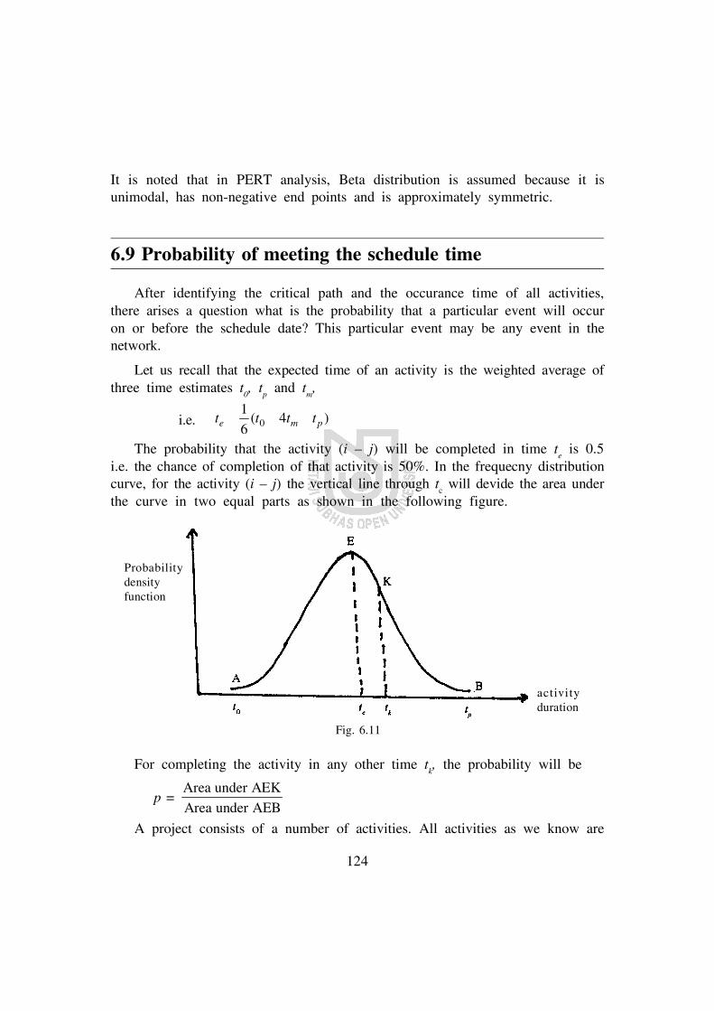
124

It is noted that in PERT analysis, Beta distribution is assumed because it isunimodal, has non-negative end points and is approximately symmetric.

6.9 Probability of meeting the schedule time

After identifying the critical path and the occurance time of all activities,there arises a question what is the probability that a particular event will occuron or before the schedule date? This particular event may be any event in thenetwork.

Let us recall that the expected time of an activity is the weighted average ofthree time estimates t

0, t

p and t

m,

i.e. 01

( 4 )6e m pt t t t? ? ?

The probability that the activity (i – j) will be completed in time te is 0.5

i.e. the chance of completion of that activity is 50%. In the frequecny distributioncurve, for the activity (i – j) the vertical line through t

c will devide the area under

the curve in two equal parts as shown in the following figure.

For completing the activity in any other time tk, the probability will be

p = Area under AEKArea under AEB

A project consists of a number of activities. All activities as we know are

Probabilitydensityfunction

activityduration

Fig. 6.11

125

independent random variables and hence the length of the project upto a certainevent through a certain path is also a random variable. But the point of differenceis the expected project length T

e does not have the same probability distribution

as the expected activity time te. While a Beta distribution curve approximately

represents the activity time probability distribution, the project expected time Te

follows approximately a standard normal distribution. This standard normaldistribution curve has an area equal to unity and standard deviation 1 and issymmetrical about the mean as follows :

Probabilitydensityfunction

activityduration

Fig. 6.12

The probility of completing a project in time Ts is given by

p(Ts) =

Area under AEKArea under AEB

The p(Ts) depends upon the location of T

s. Taking T

e as reference point the

distance Ts – T

e can be expressed in terms of standard deviation for a network is

calculated as

Standard deviation for a network

e= sum of the variances along the critical path? ?

i.e. for a network = 2ij??

where 2ij? for an activity (i – j) =

20pt t

??? ?

? ?? ?

126

Since the standard deviation for a standar normal curve is unity, the strandarddeviation

e, calculated above, is used as scale factor for calculating the normal

deviate.

The normal deviation D = s e

e

T T

Hence the probability of completing the project by scheduling time (Ts) is

given by

P(Z D) where D = s e

e

T T

??

and Z is the standard normal variate.

The values of the probabilities for a normal distribution curve correspondingto the different values of normal deviate are available from the table of standardnormal curve.

Example 2 : A small project is composed of seven activities whose timeestimates (in weeks) are listed in the following table :

Activity 1-2 1-3 1-4 2-5 3-5 4-6 5-6

t0

1 1 2 1 2 2 3

tm

1 4 2 1 5 5 6

tp

7 7 8 1 14 8 15

(a) Draw the project network.

(b) Find the expected duration and variance of each activity.

(c) Calculate the earliest and latest occurance time for each event and theexpected project length.

(d) Calculate the variance the standard deviation of project length.

(e) What is the probability that the project will be completed—

(i) at least 4 weeks earlier than expected?

(ii) Not more than 4 weeks later than expected?

(f) If the project due date is 19 weeks, what is the probability of meetingthe due date?

(g) Find also the schedule time on which the project wil be compleed witha probability 0.90.

127

Solution :

Fig. 6.13

(b) The expected time and variance of each activity is computed and displayedin the following table.

Activity t0

tm

tp

0 4

6m p

e

t t tt

? ??

202

6pt t

??? ?

? ? ?? ?

1–2 1 1 7 2 1

1-3 1 4 7 4 1

1-4 2 2 8 3 1

2-5 1 1 1 1 0

3-5 2 5 14 6 4

4-6 2 5 8 5 1

5-6 3 6 15 7 4

(c) Forward Pass calculations

Let Ei be the earliest occurance time of event i.

Set E1 = 0

E2 = E

1 + t

2 = 0 + 2 = 2

E3 = E

1 + t

13 = 0 + 4 = 4

E4 = E

1 + t

14= 0 + 3 = 3

E5 = 2,3

maxi? = max {E

2 + t

25, E

3 + t

35} = max {2 + 1, 4 + 6} = 10

E6 = 4,5

maxi? {E

i + t

i6} = max {E

4 + t

46, E

5 + t

56} = max {3 +5, 10 + 7} = 17

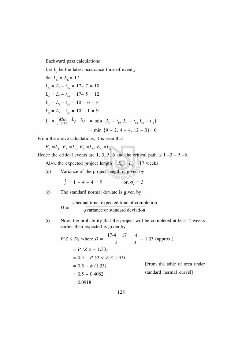
128

Backward pass calculations

Let Lj be the latest occurance time of event j

Set L6 = E

6 = 17

L5 = L

6 – t

56 = 17– 7 = 10

L4 = L

6 – t

46 = 17– 5 = 12

L3 = L

5 – t

35 = 10 – 6 = 4

L2 = L

5 – t

25 = 10 – 1 = 9

L1 = ? ?1

2,3,4j j

jMin L t?

? = min {L2 – t

12, L

3 – t

13, L

4 – t

14}

= min {9 – 2, 4 – 4, 12 – 3}= 0

From the above calculations, it is seen that

E1 =L

1, F

3 =L

3, E

5 =L

5, E

6 =L

6

Hence the critical events are 1, 3, 5, 6 and the critical path is 1 –3 – 5 –6.

Also, the expected project length = E6 = L

6 = 17 weeks

(d) Variance of the project length is given by

2e? = 1 + 4 + 4 = 9 or,

e = 3

(e) The standard normal deviate is given by

D = schedual time- expected time of completion

variance or standard deviation

(i) Now, the probability that the project will be completed at least 4 weeksearlier than expected is given by

P(Z D) where D = ? ?17-4 17 4

3 3

? ?? – 1.33 (approx.)

= P (Z – 1.33)

= 0.5 – P (0 < Z 1.33)

= 0.5 – (1.33)

= 0.5 – 0.4082

= 0.0918

[From the table of area under

standard nermal curvel]

129

(ii) Again, the probability that the project will be completed not more than4 weeks later than expected = the probability that the project will be completedwithin 17 + 4 = 21 weeks

= P (Z D) where D = 21 17 41.33

3 3? ? ?

= P (Z 1.33)

= 0.5 + (1.33)

= 0.5 + 0.4082

= 0.9082

(f) When the due date is 19 weeks, D = 19 17 2

0.673 3? ? ?

Then the probability of meeting the due dat is given by

P (Z 0.67) = 0.5 + (0.67)

= 0.5 + 0.2514

= 0.7514

(g) Since the probability for the completion of the project is 0.90, P (Z D)

= 0.90 where D = s eT T??

& Ts be the schedule time As P(Z 1.29) = 0.90

D = 1.29 which implies17

1.293

sT ? ?

i.e. Ts = 17 + 3 1.29

i.e. Ts = 20.87

130

6.10 Difference between PERT and CPM

PERT

1. This technique was developed inconnection with R & D (Research& Development) works, therefore ithad to scope with the uncertaintywhich ae associated with R & Dactivities. In this case, total projectduration is regarded as a randomvariabel. As a result, multiple timeestimates are made to calculate theprobability of completing the projectwithin the schedule time. Therefore,it is a probabilistic model.

2. It is used for projects involvingactivities of non-repetitive nature,

3. It is event oriented technuquebecause the results of analysis areexpressed in terms of events ordistinct points in time indicative ofprogress.

4. It incorporates satistical analysisthereby enables the determination ofprobabilities cocerning the time bywhich each activity and the entireproject would be completed.

5. It serves a useful control device asit assists the management incontrolling a project by callingattention through constant reviewto such delays in activities whichmight lead to a delay in the projectcompletion date.

CPM

1. This technique was developed inconnection with a constructionand maintenance project whichconsists of routine tasks or jobswhose resource requirement andduration is knwon with certainty.Therefore, it is basically adeterminnistic model.

2. It is used for projects involvingactivities or repetitive nature.

3. It is actively oriented techniqueas the results of calculations areconsidered in terms of activities.

4. It does not incorporate statisticalanalysis in determining theestimates because time is preciseand known.

5. It is difficult to use this techniqueas a controlling device for thesimple reason that one must repeatthe entire evaluation of the projecteach time the changes aeintroduced into the network.

131

6.11 Project Time-cost trade off

In this section, the cost of resources consumed by activities are taken intoconsideration. The project completion time can be reduced (crashing) the normalcompletion time of ciritical activities. The reduction in normal time of completionwill increase the total budget of the project. However, the decision-maker willalways look for trade-off between total cost of the project and total time requiredto complete it.

Project Cost : In order to include the cost aspects in project scheduling wehave to find out the cost duration relationships for various activities in the project.The total cost of any project comprises direct and indirect costs.

Direct Cost : This cost is directly dependent upon the amount of resourcesin the execution of individual activities such as manpower loading, materialconsumed etc. The direct cost increases if the activity duration is to be reduced.

Indirect Cost : This cost is associated with expenditure which can not beallocated to individual activities of the project. This cost may include managerialservices, loss of revenue, fixed overheads etc. The indirect cost is computed ona per day, per week or per month basis. This cost decreaes if the activity durationis to be reduced.

The network diagram can be used to identify the activities whose durationshould be shortened so that the completion time of the project can be shortenedin the most economic manner. The process or reducing the activity duration byputting on extra effort is called crashing the activity.

The crash time (Tc) represents the minimum activity duration time that is

possible and any attempts to further crash would only raise the activity cost withoutreducing the time. The activity cost corresponding to the crash time is called thecrash cost (C

c) which is the minimum direct cost requred to achieve the crash

Performance time.

The normal cost (Cn) is equal to the absolute minimum of the direct cost

required to perform an activity. The corresponding time duration taken by anactivity is known as the normal time (T

n).

132

The direct cost curve (from the relationship of direct cost and tiem) are shownin the figure. The point B denotes the normal time for completion of an activitywhereas the point A denotes the crash time whch indicates the least duration inwhich activity can be completed. The cost curve is non-linear and asymptoticnature. But, for the sake of simplicity, it can be approximated by a straight linewhose slope (in magnitude) is given by

c n

n c

C - CCrash cost - Normal costcost slope = =

Normal time - Crash time T -T

It is also called as crash cost slope or crash cost per unit time. This cost sloperepresents the rate of increase in the cost of performing the activity per unitreduction in time and is called cost/time trade off. It varies from activity to activity.After assessing the direct and indirect project costs, this total project cost whichis the sum of direct and indirect cost can be found out.

Time-cost optimization algorithm/Time-cost trade off procedure

The following are the steps involved in the project crashing.

Step 1. Consedering normal times of all activities, identify the criticalactivities and find the critical path.

Step 2. Calculate the cost slope for different activities and rank the activitiesin the ascending order of cost slope.

Step 3. Crash the activities on the critical path as per ranking i.e. activityhaving lower cost slope would be crashed first to the maximum ectent possible(For the crashing of lower cost slope i.e. for the reduction of activity durationtime, the direct cost of the project would increased very slowly.)

Dir

ect

Cos

t

Time

Fig. 6.14

133

Step 4. Due to the reduction of ciritical path durtion by crashing in step 3,other path may also become critical i.e. we get parallel critical paths. In suchcases, the project duration can be reduced by crashing of activities simultaneouslyin the parallel critical paths.

Step 5. Repeat the process until all the ciritical activities are fully crashedor no further crashing is possible.

In the case of indirect cost, the process of crashing is repeated until the totalcost is minimum beyond which it may increase. The minimum cost is called theoptimum project cost and the corresponding time, the optimum project time.

example 3.

The following table shows activities, their nomal time and cost and crashtime and cost for a project.

Activity Normal time Cost (Rs) Crash time Cost (Rs.)

(days) (days)

1–2 6 1400 4 1900

1-3 8 2000 5 2800

2-3 4 1100 2 1500

2-4 3 800 2 1400

3-4 Dummy — — —

3–5 6 900 3 1600

4–6 10 2500 6 3500

5–6 3 500 2 800

Indirect cost for the project is Rs. 300 per day.

(i) Draw the network of the project.

(ii) What are the normal duration and associated cost of the project?

(iii) What will be the least project duration and corresponding cost?

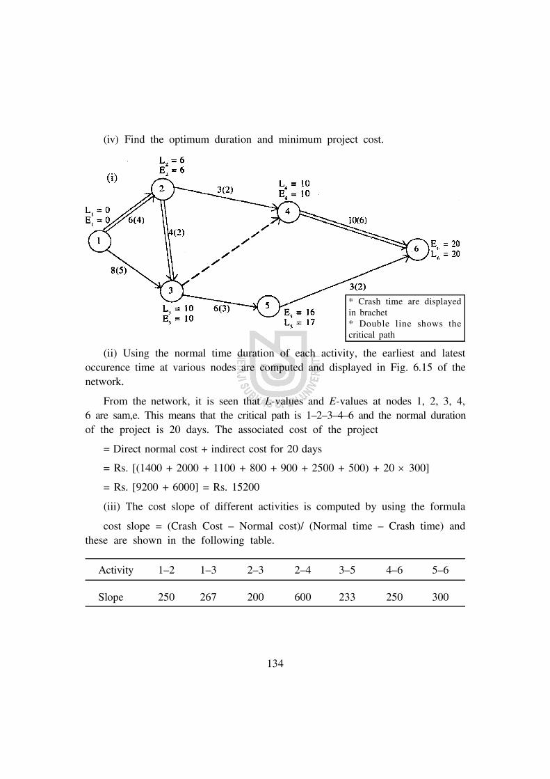
134

(iv) Find the optimum duration and minimum project cost.

Solution :

(ii) Using the normal time duration of each activity, the earliest and latestoccurence time at various nodes are computed and displayed in Fig. 6.15 of thenetwork.

From the network, it is seen that L-values and E-values at nodes 1, 2, 3, 4,6 are sam,e. This means that the critical path is 1–2–3–4–6 and the normal durationof the project is 20 days. The associated cost of the project

= Direct normal cost + indirect cost for 20 days

= Rs. [(1400 + 2000 + 1100 + 800 + 900 + 2500 + 500) + 20 300]

= Rs. [9200 + 6000] = Rs. 15200

(iii) The cost slope of different activities is computed by using the formula

cost slope = (Crash Cost – Normal cost)/ (Normal time – Crash time) andthese are shown in the following table.

Activity 1–2 1–3 2–3 2–4 3–5 4–6 5–6

Slope 250 267 200 600 233 250 300

* Crash time are displayedin brachet* Double line shows thecritical path

135

Now

we

cons

truc

t th

e fo

llow

ing

tabl

e fo

r fi

ndin

g th

e op

timal

cos

t w

ith d

urat

ion

and

min

imum

pro

ject

dur

atio

nw

ith c

ost.

Cri

tical

Pat

h (s

)S

eeA

ctiv

itie

sP

roje

ctN

orm

alC

rash

ing

cost

(R

s.)

Indi

rect

cos

tT

otal

cos

tF

igur

ecr

ashe

dle

ngth

dire

ct c

ost

(B)

(Rs.

300

/day

)(R

s.)

& t

ime

(day

s)(R

s.)

(A)

(C)

(A+B

+C)

1-2-

3-4-

6Fi

g. 6

.15

—2

09,

200

—30

0 ×

2015

200

1-2-

3-4-

6D

o2–

3 (1

)1

99,

200

200

× 1

= 20

030

0 ×

1915

100

1-2-

3-4-

6Fi

g. 6

.16

1-2(

1)1

89,

200

200

+ 25

0 ×

.1 =

450

300

× 18

1505

01-

2-4-

6

1-2-

3-4-

6Fi

g. 6

.17

4-6(

1)1

79,

200

450

+ 25

0×

1=70

030

0 ×

1715

000

1-2-

4-6

1-3-

4-6

1-2-

3-4-

6Fi

g. 6

.18

3-5(

1)1

69,

200

700+

233

× 1

+ 25

0 ×1

300

× 16

1518

31-

2-4-

64-

6(1)

= 11

831-

3-4-

6 &

1-3-

5-6

Do

Fig.

6.1

93-

5(1)

15

9,20

011

83 +

233

×1+

250×

130

0 ×

1515

366

4-6(

1)=

1626

Do

Fig.

6.2

03–

5(1)

14

9,20

016

26+

233

×1+

250×

130

0 ×

1415

549

4-6(

1)=

1626

Do

Fig.

6.2

11–

2(1)

13

9,20

021

09+

250×

1+26

7 ×

130

0 ×

1315

766

1-3(

1)=

2626

Do

Fig.

6.2

22–

3(1)

12

9,20

026

26+

250×

1+60

0 ×

130

0 ×

1216

493

2–4(

1)=

2626

1-3(

1)

136

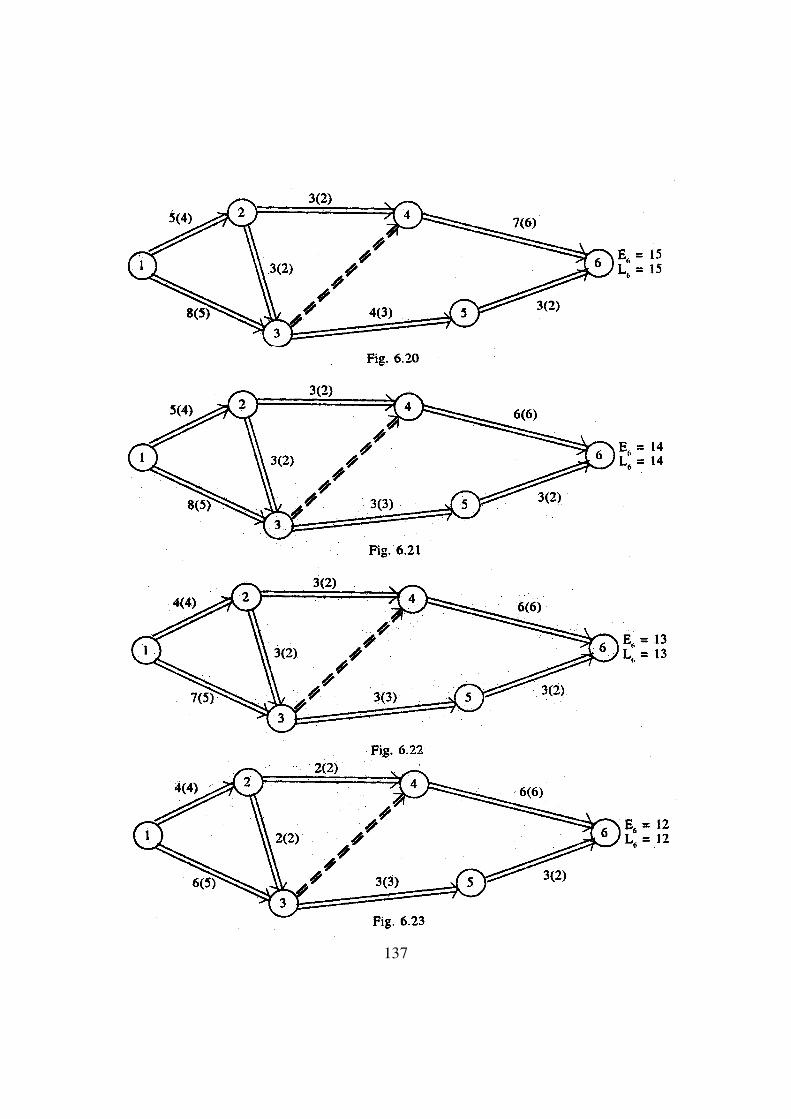
137

138

From Fig. 6.23, it is seen that no further crashing is possible beyond 12days. Hence the least project duration is 12 days and the corresponding cost ofthe project will be Rs. 16493.00

(iv) As the minimum cost occurs for 17 days schedule, optimum duration ofthe project is 17 days and the minimum project cost is Rs. 15000.00

6.12 Summary

In this unit, the network analysis of a project has been discussed. For thispurpose, two very popular techniques i.e. CPM and PERT analysis have beenexplained clearly. Finally, considering the considering the cost aspects in a project,time cost trade off algorithm has been focussed. To illustrat the different techniques,some numerical examples have been solved showing the different steps.

6.13 Exercise

1. A project consists of a series of tasks lebellel A, B, ...., H, I, with thefollowing relationships (W < X, Y means X and Y can not start until W iscompleted; X, Y < @ means W can not start until both X and Y are completed).With this notation construct the network diagram having the following constraints:

A < D, E; B, D < F; C < G; B, G < H; F, G < 1

Find also the minimum time of completion of the project, when the time (in days)of completion of each task is as follows :

Task : A B C D E F G H I

Time : 23 8 20 16 24 18 19 4 10

2. The following are the detains of estimated times of activities of a certain project.

Activity : A B C D E F

Immediate

Predecessor : — A A B,C — E

Estimated time : 2 3 4 6 2 8

(weeks)

139

(a) Find the critical path and the expected time of the project.

(b) Calculate the earliest start time and earliest finish time for each activity.

(c) Calculate the slack for each activity.

3. Draw the network for the following project anc compute the earliest and latesttimes for each event and also find the ciritcal path :

Activity : 1-2 1-3 2-4 3-4 4-5 4-6 5-7 6-7 7-8

ImmediatePredecessor : — — 1-2 1-3 2-4 2-4 & 3-4 4-5 4-6 6-7&5-7

Time (days ) : 5 4 6 2 1 7 8 4 3

4. A project consists of eight activities with the following relevant information :

Activity Immediate Estimated duration (days)

prodecessor Optimistic Most likely Pessimistic

A — 1 1 7

B — 1 4 7

C — 2 2 8

D A 1 1 1

E B 2 5 14

F C 2 5 14

G D, E 3 6 15

H F, G 1 2 3

(i) Draw the network and fined out the expected project completion time.

(ii) What duration will have 95% confidence for project completion?

(iii) If the average duration for activity F increases to 14 days, what willbe its effectts on the expected project completion time which will have 95%confidence?

140

5. A small project consists of seven activities, the details of which are givenbelow :

Activity Time estimates Predecessor

t0

tm

tp

A 3 6 9 None

B 2 5 8 None

C 2 4 6 A

D 2 3 10 B

E 1 3 11 B

F 4 6 8 C, D

G 1 5 15 E

Find the critical path. What is the probability that the project will be competed by18 weeks?

6. The following table gives data or normal time-cost and crash time-cost for aproject :

Activity Normal Crash

Time (days) Cost (Rs.) Time (days) Cost (Rs.)

1–2 6 650 4 1000

1–3 4 600 2 2000

2–4 5 500 3 1500

2–5 3 450 1 650

3–4 6 900 4 2000

4–6 8 800 4 3000

5–6 4 400 2 1000

6–7 3 450 2 800

141

7. The following table gives the activities in a construction project and otherrelevant information.

Activity Immediate Time (days) Direct cost (Rs.)

Predecessor Normal Crash Normal Crash

A — 4 3 60 90

B — 6 4 150 250

C — 2 1 38 60

D A 5 3 150 250

E C 2 2 100 100

F A 7 5 115 175

G B, D, E 4 2 100 240

Indirect costs vary as follows :

Days : 15 14 13 12 11 10 9 8 7 6

Cost (Rs.) : 600 500 400 250 175 100 75 50 35 25

(i) Draw an arrow diagram for the project.

(ii) Determine the project duration which will result in minimum total projectcost.

6.14 References

1. H. A. Taha, Operations Research, An Intorduction, PHI, India.

2. Swarup, Gupta & Mohan, Operations Research, Sultan Chand & Sons, India.

3. S. D. Sharma, Operations Research, Kedar Nath Ram Nath & Co., India.

142

Unit 7 p Inventory Management

Structure

7.0 Objectives

7.1 Introduction

7.2 Types of Inventory

7.3 Basic concepts and Terminologies in inventory

7.3.1 Demand

7.3.2 Replenishment

7.3.3 constraints

7.3.4 Fully backlogged/Partially backlogged shortages

7.3.5 Lead time

7.3.6 Planning/time Horizon

7.3.7 Deterioration / Damagability / Perishability

7.3.8 Various types of inventing costs

7.4 Classification of inventory models

7.4.1 Model-1

7.4.2 Model-2

7.4.3 Model-3

7.4.4 Model-4

7.5 Multi-item Deterministic Problem

7.6 Limitation on Invention

7.6.1 Limitation of flour space

7.6.2 Limitation on Investment

7.7 Inventory models with price breaks

7.7.1 Purchasing inventory model with single price break

7.7.2 Purchase inventory model with two price breaks

7.8 Probabilistic Inventory Model

7.8.1 Single period model with uniform model

7.8.2 Single period inventory model with discontinuous demand.

143

7.0 Objectives

In real life, it is observed that a small retailer knows roughly the demand ofhis/her customes, in a year or a month or a week and accordingly, places orderson the whosesaleer to meet the demand of his/her customers. But, this is notpossible for the authority/management of large production firms/deparmental stores/shops.

The reason behind this is that the stocking of items in such cases dependsupon the various factors e.g., demand of an item, ordering time, time lag betweenorders and actual receiving (i.e., Lead time) etc. So the problem for managers/retailers is to have a compromise between overstocking and under-stocking. Thestudy of such type of problems is known as Inventory Control (IC). The IC maybe defined as the function of directing the movement of goods through the entiremanufacturing cycle from the requisitioning of raw materials to the inventory offinished goods in orderly mannered to meet up the objectives of maximumcustomer-service with minimum investmnet and efficient (low-cost) plant operation.

In this unit, we shall introduce only the inventory models of elementary typefor deterministic and probabilistic cases. These are single item purchasing andmanufacturing model with/without shortages, price breaks models, multi-itempurchasing model with different constraints like investment, average inventory andspace constraints. Also, we shall introduce probabilistic models for discrete (wellknown News boy problem) and continuous cases. This discussion will help us toderive the real life purchasing/manufacturing inventory models.

7.1 Introduction

In broad sense, inventory is defined as an idle resource of an enterprise/company/manufacturing firm. It can be defined as a stock of physical goods,commodities or other economic resources which are used to meet up the customer’sdemand or requirement of production. This means that the inventory acts a bufferstock between a supplier and a customer.

144

The inventory or stock of goods may be kept in any one of the followingforms.

(i) raw materials

(ii) semi-finished goods (work-in-process inventory)

(iii) finished (or produced) goods

(iv) maintenance, repair and operating supplies (MRO) items.

In any sector of an economy, the control and maintenance of inventory isa problem common to all organisations. Inventories of physical goods aremaintained in governemnt and non-government establishments e.g., Agriculture,Industry, Military, Business, etc. Some reasons for maintaing inventories are asfollows :

(i) to conduct smooth and efficient running of business.

(ii) to provide the customer service by meeting their demands from stockwithout delay.

(iii) to earn price discount for bulk purchasing.

(iv) to maintain more stable operating and/or work force levels.

(v) to take the financial advantage of transporting/shipping economics.

(vi) to plan overall operating strategy through decoupling of succesive stagesin the chain of acquireing goods, preparing products, shipping to branchware houses and finally serving the customers.

(vii) to motivate the customers to purchase more by displaying large numberof goods in the showroom/shop.

(viii) to take the advantages in purchashing of some raw materials and somecommonly used physical goods (such as paddy, wheat etc.) whose pricesseasonally fluctuate. In this connection, it is more profitable to procurea sufficient quantity of these raw materials/commonly used physical goodswhen their prices are low to be used later during the high price seasonor when need arises.

Production/Inventory planning and control is essentially concerned with thedesing-operation and control of an inventroy system in any sector of a given

145

economy. The problem of inventory control is primarily concerned with thefollowing fundamental questions :

(i) whick items should be carried in stock? or which items should beproduced?

(ii) How much of each of these items should be ordered/produced?

(iii) when should an order be placed? or when to produce?

(iv) what type of inventory control system should be used?

In practice, it is a formidable task to determine a suitable inventory policy.Regarding the above mentioned questions, an inventory problem is a problem ofmaking optimal decisions. In other words, an inventory problem deals with decisionsthat optimize either the cost function (total or average cost) or the profit function(total or average profit) of the inventory system. However, there are certain typesof problems, such as those relating to the storage of water in a dam in whichone has no control over the replenishment of inventory. The supply of inventoryof water in a dam depends on rainfall and the organisation operating the dam,has no contorl over it.

Our aim is to formulate mathematical models of different inventory controlsystems and to solve those using different mathematical analysis. For this purpose,our task is to construct a mathematical model of the inventory system. However,this type of model is biasc on different assumptions and approximations. It isdifficult both to devise and operate with an exact/accurate model. We do notknow what the real world is. Therefore, it is almost impossible to construct arealistic model with complete accuracy. For this reason, some approximations andsimplifications must be used during the model building process. Again, the solutionof the inventory problem is a set of specific values of variables that minimizesthe total (or average) cost of the system or maximizes the total (or average) profitof the system.

7.2 Types of Inventory

There are five types of inventory, namely :

(i) Transportation inventories, (ii) Fluctuaton inventoreis.

146

(iii) Anticipation inventories, (iv) De-coupling inventoreis, (v) Lot-sizeinventories.

Transportation inventories : This arises due to transportaion of inventoryitems to various distribution centres and customers from the various productioncentres, when the transportation time is long, the items under transport can notbe served to customers. These inventories exist solely because of transportationtime.

Fluctuation inventories : These have to be carried because sales andproduction times can not be predicted accurately. In real-life problems, there arefluctuations in the demand and lead-times that affect the production of items.

Anticipation inventoreis : These are build up in advance by anticipating orforeseeing the future demand for the season of large sales, a promotion programmeor a plant shout-down period.

De-coupling inventories : The inventories used to reduce the inter dependanceof various stages of production system are known as de-coupling inventories.

Lot-size inventories : Generally, the rate of consumption is different fromthe rate of production or purchasing. Thereofre, items are produced in largerquantities which result in lot-size, also called as cycle inventories.

7.3 Basic concepts and Terminologies in Inventory

The inventory systems depend on several system factors and parameterssuch as demand, replenishment rate, shortages, constraints, various types of costsetc.

7.3.1 Demand

Demand is defined as the number of units of an item required by the customer ina unit time and has the dimension of a quantity. It may be known exactly or knownin terms of probabilities or may be completely unknown.

The demand pattern of items may be either deterministic or probabilistic. Problemin which demand is known and fixed are called deterministic problem. Whereas thoseproblems in which the demand is assumed to be a random variable are called stochasticor probabilistic problems.

147

In case of deterministic demand it is assumed that the quantities needed oversubsequent periods of time are known exactly. Further, the known demand may befixed or variable with time or stock-level or selling price of an item etc.

Probabilistic demand occurs when requirements over a certain period of timeare not known with certainty but their pattern can be described by a knownprobability distribution.

In some cases, demand may also be represented by uncertain data in non-stochastic sense i.e., by vague/imprecise data. This type of demand is termed asfuzzy demand and the system as a fuzzy system.

7.3.2 Replenishment

Replenishment refers to the amount of quantities that are scheduled to be putinto inventories, at the time when decisions are made about ordering these quantitiesor to the time when they ae actually added to stock. It can be categorizedaccording to size, pattern and lead time. Replenishment size may be constant orvariable, depending upon the type of the inventory system. It may depend ontime, demand and/or on-hand inventory level. The replenishment patterns areusually instantaneous, uniform or in batch. The replenishment quantity again maybe probabilistic or fuzzy in nature.

7.3.3Constraints

Constraints are the limitations imposed on the inventory system. It may beimposed on the amount of investment, available space, the amount of inventoryheld, average instantaneous expenditure, number of orders, etc.

7.3.4 Fully backlogged/ Partially backlogged Shortages

During stock out period, the sales or goodwill may be lost either by a delayor complete refusal in meeting the demand. If the unfulfilled demand for thegoods is satisfied completely at a later date, then it is a case of fully backloggedshortage i.e. it is assumed that no customer balk away during this period and thedeamnd of all these waiting customers is met up at the beginning of the nextperiod gradually after the commencement of next production.

Again, it is normally observed that during the stock out period, some of thecustomers wait for the product and toher balk away. When this happens, thephenomenon is called partially backlogged shortages.

148

7.3.5 Lead time

The time gap between the time of placing an order or production start andthe time of arrival of goods in stock is called the lead time. If may be a constantor a variable. Again, variable lead time may be probabilistic or imprecise.

7.3.6 Planning/Time Horizon

The time period over which the inventory level will be controlled is called thetime/planning horizon. It may be finite or infinite depending upon the nature of theinventory system ofr the commodity.

7.3.7 Deterioration/Damagability/Perishability

Deterioration is defined as decay, evaporation, obsolescence and loss of utilityor marginal value of a commodity that results in the decreasing usefulness fromthe original condition. Vegetables, food grains and semiconductor chips, etc. areexmaples of such products.

Damagability is defined by the damage when the items are broken or loosetheir utility due to the accumulated stress, bad handling, hostile environment etc.The amount of damage by the stess varies with the size of stock and the durationfor which the stress is applied. Items made of glass, china-clay, ceramic, mud ec.are examples of such products.

Perishable items are those which have finite life time (fixed or random). Fixedlife time product (e.g., human blood, etc.) has a deterministic self life while therandom life time scenario is closely related to the case of an inventory whichexperiences continuous physical depletion due to deterioration or decay.

7.3.8 Various types of Inventory Costs

Inventory costs are the costs associated ith the operation of an inventorysystem and result from action or lack of action on the part of management inestablishing the system. They are basic economic parameters to any inventorydecision model.

Purchase or Unit cost : The purchase or unit cost of an item is the unitpurchase price to obtain the item from an external source or the unit productioncost for the internal production. It may also depend upon the demand. Whenproduction is done in large quantities, it results in reduction of production cost

149

per unit. Also, when quantity discounts are allowed for bulk orders, unit price isreduced and dependent on the quantity purchased or ordered.

Ordering/set up cost : The ordering or set up cost originates from theexperience of issuing a purchase order to an outside supplier or from an internalproduction set up costs. The ordering cost includes clerical and administrative costs,telephone charges, telegrams, transportation cost, loading and unloading cost etc.Generally, this cost is assumed to be independent of the quantity ordered for orproduced. In some cases, it may depend on the quantity of goods purchasedbecause of price break or quanitity discounts or transportation cost, etc.

Holding or carrying cost : The holding or carrying cost is the cost associatedwith the strorage of the inventory until its use or sale. It is directly proportionalto the amount/ quantity in the inventory and the time for which the stocks areheld. This cost generally includes the costs such as insurance, taxes, obsolescence,deterioration, rent of warehouse, light, heat, maintenance and interest on the moneylocked up.

Shortage cost or stock-out cost : The shortage cost or stock-out cost is thepenalty incurred for being unable to meet up a demand when it occours. Thiscost arises due to shortage of goods, lost sales for delay in meeting up the demandor total inability to meet up the demand. In the case, where the unfulfilled demandfor the goods can be satisfied a latter date (back logging case), this cost dependson the shortage quantity and delaying time both. On the other hand, if theunfulfilled demand is lost (no backlogging case), shortage cost becomes proportionalto the shortage quantity only. In both cases, there is a loss of goodwill whichcan not be quantified for the development of mathematical model.

Disposal cost : When an amount of some units of an item remains excessat the end of inventory cycle and if this amount is sold at a lower price in thenext cycle to derive some advantages like clearing the stock, winding up thebusiness, etc., the revenue earned through such a process is called the disposalcost.

Salvage value : During storage, some units are partially spoiled or damangedie., some units loose their utility partially. In a developing country, it is normallyobserved that some of these are sold at a reduced price (less than the pruchaseprice) to a section of customers and this gives some revenue to the management.This revenue is called salvage value.

150

7.4 Classification of inventory Models

The inventory problems (models) may be classified into two categories.

(i) Deterministic inventory models : These are the inventory models inwhich demand is assumed to be known constant or variable (dependenton time, stock-level, selling price of the item, etc.). Here, we shallconsider deterministic inventory models for known constant demand.Such models are usually referred to as beconomic lot-size models orEconomic order Quantity (EOQ) models.

There are four types of models under this category, namely

(a) Purchasing inventory model with no shortages.

(b) Manufacturing inventory model with no shortage.

(c) Purchasing inventory model with shortages.

(d) Manufacturing model with shortages.

(ii) Probabilistic inventory models : These are the inventory models inwhich the demand is a random variable having a known probabilitydistribution. Here, the future demand is determined by collecting datafrom the past experience.

7.4.1 Model-1 : The economic lot-size model (EOQ model with no shortages &instantaneous production) or Purchasing inventory model with no shortages.

In this models, we want to derive the formula for the optimum order quantityper cycle of a single product so as to minimize the total average cost under thefollowing assumptions and notations :

(i) Demand is deterministic and uniform at a rate D units of quantity perunit time.

(ii) Production is instantaneous (i.e., production rate is infinite)

(iii) Shortages are not allowed.

(iv) Lead time is zero.

(v) The inventory planning horizon is infinite and the inventory systeminvolves only one item and one stocking point.

151

(vi) Only a single order will be placed at the beginning of each cycle andthe entire lot is delivered in one batch.

(vii) The inventory carrying cost, C1 per unit quantity per unit time, the ordering

cost, C3 per order are known and constant.

(viii) T be cycle length and Q be the ordering quantiy per cycle.

inventory level

Time

Fig. 7.1

Let us assume that an enterprise purchases an amount of Q units of item attime t = 0. This amount will be depleted to meet up the customer’s demand.Ultimately, the stock level reaches to zero at time t = T. The inventory situationis shown in the Fig.1.

Clearly, Q = DT ......... (1)

Now, the inventory carrying cost for the entire cycle T is C1 (area of AOB)

= C1. QT =

12

C1QT and the ordering cost for the said cycle T is C

3.

Hence the total cost for time T is given by

X = C3 +

12

C1QT

Therefore, the total average cost is given by

C(Q) = XT

or, C (Q) = 3CT

+ 12

QC1

152

or, C(Q) = 3

112

C DC Q

Q?

Q DT

QT

D

?? ?? ?? ?? ?? ?? ?

...... (2)

The optimum value of Q which minimizes C(Q) is obtained by equating the firstderivative of C(Q) with respect to Q to zero

i.e., 0dCdQ

? or, 12

C1 –

32

0C D

Q?

or,3

1

2C DQ

Q?

Again, 2

32

2( ) C Dd C QQdQ

? which is +ve for 3

1

2C DQ

Q? .

Hence C(Q) is minimum for which the optimum value of Q is

Q* = 3

1

2C DC ...... (3)

This is known as economic lot size formula or EOQ. The corresponding optimum

time interval is T* = 3

1

2* CQD C D

? and the minimum cost per unit time is given by

3min 1 1 3

1* 2

* 2C D

C C Q C C DQ

? ? ?

This model was first developed by Ford Haris of the westing house corporation,USA, in the year 1915. He derived the well-known classical lot size formula (3). Thisformula was also developed independently by R. H. Wilson after few years and it hasbeen named as Haris-Wilson formula.

Remark :

(i) The total inventory time units for the entire cycle T is 12

QT, so the

average inventory at any time is 12

1

.2

QTQ

T?

(ii) Since C1 > 0 from f(Q) =

12

C1Q it is obvious that the inventory carrying

153

cost is a linear function of Q with a + ve slope i.e., for smaller average inventory, the

inventory carrying costs are lower. In contrast g(Q) = 3C DQ i.e., ordering cost increases

as Q decreases.

(iii) In the above model, if we always maintain an inventory B on hand as buffer

stock, then the average inventory at any time is 12

Q + B. Therefore, the total cost

per unit time is

C(Q) = 3

112

C DQ B C

Q? ?? ?? ?? ?

As before, we obtain Q = Q* = 3

1

2C DC and T = T* =

3

1

2CDC

(iv) In the above model, if the ordering cost is taken as C3 + bQ, (where b is the

purchase cost per unit quantity) instead of fixed ordering cost then there is no changein the optimum order quantity.

Proof : In this case, the average cost is given by

C(Q) = 12

C1Q +

DQ (C

3 + bQ) ....... (4)

The necessary condition for the optimum of C (Q) in (4), we have

c (Q) = 0 implies Q = 3

1

2C DC

and c (Q) >0. Hence Q* = 3

1

2C DC

This shows that there is no change in Q* in spite of change in the orderingcost.

Example 1. An engineering factory consumes 5000 units of a component peryear. The ordering, receiving and handling costs are Rs. 300 per order while thetrucing cost are Rs. 1200 per order. Interest cost Rs. 0.06 per unit per year,Deterioration and obsolence cost Rs. 0.004 per unit per year, storage cost Rs.1000.00 per year for 5000 units. Calculate the economic order quantity.

154

Solution : In the given proble, we have demand (D) = 5000 units

Ordering cost / Replenishment cost = Ordering, receiving, handling costs andtrucing costs = Rs. (300 + 1200) = Rs. 1500 per order.

Inventory carrying cost = interest costs + Deterioration and obsolence costs stroage

costs = 1000

0.06 0.0045000

? ?? ?? ?? ? rupees per unit per year.

= 0.264 rupees per unit per year.

Hence the economic order quanitity is given by

Q* = 3

1

2 2 1500 50000.264

C DC

? ??

= 7538 units (approx.)

7.4.2 Model-2 : Manufacturing model with no shortages or Economic lot-sizemodel with finite rate of replenishment and without shortages.

In this model, we shall derive formula for the optimum prodution quantity (Economiclot-size) per cycle of a single product so as to minimize the total average cost underthe following assumptions and notations :

(i) Demand is deterministic and uniform at a rate D units of quantity perunit time.

(ii) Shortages are not allowed.

(iii) Lead time is zero.

(iv) The production rate or replenishment rate is finite, say, K units per unittime (K > D).

(v) The production-inventory planning horizon is infinite and the productionsystem involves only one items and one stocking point.

(vi) The inventory carrying cost, C1 per unit quantity per unit time, the setup

cost C3 per production cycle are known and constant.

(vii) T be the cycle length and Q be economic lot-size.

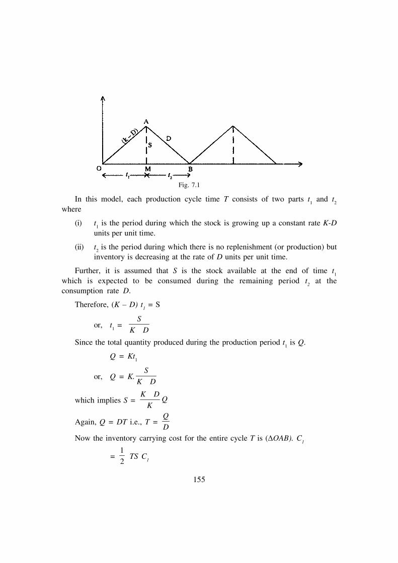
155

In this model, each production cycle time T consists of two parts t1 and t

2

where

(i) t1 is the period during which the stock is growing up a constant rate K-D

units per unit time.

(ii) t2 is the period during which there is no replenishment (or production) but

inventory is decreasing at the rate of D units per unit time.

Further, it is assumed that S is the stock available at the end of time t1

which is expected to be consumed during the remaining period t2 at the

consumption rate D.

Therefore, (K – D) t1 = S

or, t1 =

SK D?

Since the total quantity produced during the production period t1 is Q.

Q = Kt1

or, Q = K.S

K D?

which implies S = K D

QK?

Again, Q = DT i.e., T = QD

Now the inventory carrying cost for the entire cycle T is (OAB). C1

= 12

TS C1

Fig. 7.1

156

and the set-up cost for time period T is C3. Therefore, the total cost for the entire

cycle T is given by X = C3 +

12

C1

12

ST.

Therefore the total average cost is given by

C(Q) = XT

or, C (Q) = 31

12

CC S

T?

or, C (Q) = 3

112

C D K DC Q

Q K??

Q DTand

K DS Q

K

? ?? ?? ??? ??? ?? ?

The optimum value of Q which minimizes C(Q) is obtained by equation the firstderivative of C (Q) with respect to Q to zero

i.e., 0dCdQ

?

3

12

10

2C D K D

CKQ

?? ? ?

3

1

2.

C DKQ

C K D?

?

Again, 2

32 3

2C Dd C

dQ Q? = + ve quantity for Q =

3

1

2.

C DKC K D?

Hence C (Q) is minimum for which the optimum value of Q is

Q* = 3

1

2.

C DKC K D?

The corresponding time interval is

T* = 3 3

1 1

2 2*. /

( )C C KQ DK

DD C K D C D K D

? ?? ?

and the minimum average cost is given by

157

Cmin

= * 3

1 *

12

C DK DC Q

K Q

? ?

= 1 32K D

C C DK?

Remark : (i) For this model, Q*, T* and CMIN

can between in the followingform :

Q* = 3

1

2 1,

1

C DDCK

? T* = 3

1

2 1.1

CDDCk

?

and Cmin

= 1 32 1D

C C DK

? ??? ?? ?If K i.e., the production rate is infinite, this model reduces to model 1.

When k , then Q*, T* and Cmin

reduce to the expression for Q*, T* and Cmin

of model-1.

Example : A contractor has to supply 20,000 units per day. He can produce30,000 units per day. The cost of holding a unit in stock is Rs. 3.00 per year and thesetup cost per run is Rs. 50.00. How frequently and of what size, the production runsbe made?

Solution : For this problem, it is given that

D = 20,000 units / day

K = 30,000 units / day

C1

= Rs. 3.00 per year = Rs. 3

365 per day

C1

= Rs. 50.00 per run

Let Q* be the optimum lot-size.

Q* =3

1

2 1

1

C DDCK

?

=

2 50 20000 13 20000

1365 30000

? ?

? units

158

= 2 50 20000 365 3

3? ? ? ?

= 2 50 20000 365? ? ? units

= 27019 units

Let T* be the optimal cycle length

T* = * 27019

20000QD

? days = 1.35 days

Length of production cycle = 2701920000

= 0.9 days.

Thus the production cycle starts at an interval of 1.35 days and production continuesfor 0.9 days so that in each cycle a batch of 27019 units is produced.

7.4.3 Model-3 : Purchasing model with shortages

In this model, we shall derive the optimal order level and the minimum averagecost under the following assumptions and notations :

(i) Demand is deterministic and uniform at a rate D units of quantity per unittime.

(ii) Production is instantaneous (i.e., production rate is infinite).

(iii) Shortages are allowed and fully backlogged.


(v) The inventory planning horizon is infinite and the inventory system involvesonly one items and one stocking point.

(vi) Only a single order will be placed at the beginning of each cycle and theentire lot is delivered in one batch.

(vii) The inventory carrying cost, C1 per unit quantity per unit time, the shortage

cost, C2 per unit quantity per unit time, the ordering cost, C

3 per order are

known and constant.

(viii) Q be the lot-size per cycle where as S is the initial inventory level afterfulfiling the backlogged quantity of previous cycle and Q – S be the maximumshortage level.

(ix) T be the cycle length or scheduling period whereas t1 be the no shortage

period.

159

According to the assumption of (viii) & (ix), we have Q = DT. Regardingthe cycle length or scheduling period of the inventory system, two cases mayarise :

Case-1 : Cycle length or scheduling peirod T is constant.

Case-2 : Cycle length or scheduling period T is a variable.

Case-3 : In this case, T is constant i.e., inventory is to be replenished after everyfixed time period T.

As t1 be the shortage peirod, S = Dt

1 in t

1 =

SD

. Now, the inventory carrying cost

during the period O to t1 is

C1 (Area of OAB)

= 12

C1St

1 =

12

C1

2SD

Again the shortage cost during the interval (t1, T) is

C2 (Area of ACD)

= 12

C2 (Q – S) (T – t

1)

= 12

C2 (Q – S)2 /D 1

Q ST t

D?? ?? ?? ?? ?

Hence the total average cost of the system is given by

inve

ntor

y

Time

Fig. 7.3

160

C = ? ?22

3 1 21 1

/2 2

Q SSC C C T

D D

? ??? ?? ?? ?? ?

........ (1)

Since T is constant, Q = DT is also constant. Hence the above expression i.e., theexpression for average cost is a function of single variable S. So, we can easilyminimize the above expression (1) with respect to S like model-1.

In this case, S* = 2 2

1 2 1 2

C Q C DT

C C C C?

? ?

and Cmin

= 1 2 1 2

1 2 1 2

C C Q C C DT

C C C C?

? ?

Case-2 : In this case, cycle length or scheduling period T is a variable. Like case-1, in this case, the average cost of the inventory system will be

C = C = ? ?22

3 1 21 1

/2 2

Q SSC C C T

D D

? ??? ?? ?? ?? ?

..... (2)

where Q = DT

Here, the average cost C is a function of two independent variables T and S1.

Now, for optimal value of C, we have

1

c

s

?? = 0 and

cT

?? = 0

(ii) If C2 and C

1 > 0. then shortages are prohibited. In this case, S*

1 = Q*

= 31

2D

CC and each batch Q* is used entirely for inventory.

(iii) If shortage costs are negligible, then C1 > 0 and C

2 . 0. In this case, S*

1

and Q* .

(iii) If inventory carrying costs are negiligible, then C1 > 0 and C

2 > 0. In this case,

Q* .

(iv) If inventory carrying costs are negligible, then C1 0 and C

2 0. In

this case, Q* and S*1 i.e., S*

1 Q*. Thus, due to very very small

inventory carrying costs, large lot-size should be ordered and used to meet up thefuture demand.

161

(v) When in every carrying costs and shortage costs are equal i.e., when C1 = C

2,

1

1 2

12

C

C C?

? .

In this case, Q* = 3

1

2 2C DC

Whick shows that the lot-size is 2 times of the lot size of case-1 model i.e., whenno shortages are allowed.

Example-2 : The demand for an item is 18000 units per year. The inventorycarrying cost is Rs. 1.20 per unit time and the cost of shortage is Rs. 5.00. Theordering cost is Rs. 400.00. Assuming that the replenishment rate is instantaneousdetermine the optimum order quanity, shortage quantity and cycle length.

Solution : For the prolem, It is given that elemtnf D = 180000 units per year,carrying cost C

1 = Rs. 1.20 per unit, shortage cost C

2 = Rs. 5.000, ordering cost C

3

= Rs. 400 per order.

1

0C

S

? ??

gives S1 = 2

1 2( )DT

CC C? ..... (3)

Again, CT

?? = 0

? ?221 31 1 1 2

22 2 20

2 2

DT S CC S DT S CC

D T DT T T

??? ? ? ? ?

putting S1 = 2

1 2( )DT

CC C? in above and simplifying, we have

T = T* =3 1 2

1 2

2 ( )C C CC C D

?..... (4)

Then S1 = S*

1 =

2 3

1 1 2

2( )C C D

C C C? ..... (5)

Obviously, for the volumes of T and S1 given by (4) & (5),

2

21

0,C

S

? ??

2

20

S

T

? ??

and

22 2 2

1 1

0C C C

S T S T

? ?? ? ?? ?? ?? ?? ? ? ?? ?

162

Hence C is minimum for the values of T & S1 given by (4) and (5).

Therefore the optimum order quantity for minimum cost is given by

Q* = DT* = D 3 1 2 3 1 2

1 2 1 2

2 ( ) 2 ( )C C C C C C DC C D C C

? ?? ..... (6)

and Cmin

= C* = 1 2 3

1 2

2( )C C C DC C? ..... (7)

Remark :

(i) If C1 and C

2 > 0, inventories are prohibited. In this S*

1 = 0 and Q* =

3

2

2C DC and each lot-size is used to fill the back orders.

The optimum order quantity Q* is given by

Q* = 3 1 2

1 2

2 ( ) 2 400 (1.2 5) 180001.2 5

C C C DC C

? ? ? ? ?? ??

3857 units

Again, the optimum shortage quantity Q* – S*1 =3857 –

2 3

1 1 2

2( )C C D

C C C?

= 3857 – 2 5 400 18000

1.2 (1.2 5)? ? ?

? ?

= 746 units.

Optimal cycle length T* = * 3857

0.21418000

QD

? ? year.

Example-3 : The demand for an item is deterministic and constant over time andit is equal to 600 units per year. The per unit cost of the item is Rs. 50.00 while thecost of placing an order is Rs. 5.00> The inventory carrying cost is 20% of the unitcost of the item and the shortage cost per month is Rs. 1. Find the optimal orderingquantity. If shortages are not allowed, what would be the loss of the company.

Solution : It is given that D = 600 units / year

C1 = 20% of Rs. 50.00 = Rs. 10.00

163

C2 = Re 1 per month i.e., Rs. 12 per year.

C3 = Rs. 5 per order.

(i) when shortages are allowed.

The optimal ordering quantity Q* is given by

Q* = 3 1 2

1 2

2 ( )C C C DC C

?= 33 units.

and the minimum cost per year is

1 2 3

1 2

2( *)

( )C C C D

C QC C

? ??

Rs. 180.91

If shortages ae not allowed, then the optical order quantity is

Q* = 3

1

224.5

C DC

? units

and the relevant average cost is given by

C(Q*) = Rs. 1 32C C D = Rs. 244.95

Therefore, if shortages are not allowed, the loss of the company will be Rs.(244.95 – 180.91) i.e., Rs. 64.04.

7.4.4 Model-4 : Manufacturing model with shortages or Economic lot-sizemodel with finite rate of replenishment and shortages.

In this model, we shall derive the formula for the optimum production quantity,shortage quantity anc cycle length of a single product by minimizing the average costof the production system under the following assumptions and notations :

(i) The production rate or replenishment rate is finite, say K units per unit time(K>D).

(ii) The production-inventory planning horizon is infinite and the productionsystem involves only one item and one stockig point.

(iii) Demand of the item is deterministic and uniform at a rate D units of quantityper unit time.

164

(iv) Shortages are allowed.

(v) Lead time is zero.

(vi) The inventory carrying cost, C1 per unit quantity per unit time, the shortage

cost, C2 per unit quantity per unit time and the set up cost, C

3 per set up are

known and constant.

(vii) T be the cycle length of the system i.e., T be the interval between productioncycles.

(viii) Q be the economic lot-size.

inve

ntor

y le

vel

Fig. 7.4

Let us assume that each production cycle of length T consists of two partst12

and t34

which are further subdivided inti t1 and t2; t

3 and t

4 where (i) inventory

is building up at a constant rate K – D units per unit time during the interval[0, t

1] (ii) at time t = t

1, the production is stopped and the stock level decreases

due to meet up the customers, demand only upto the time t = t1 + t

2. (iii) shortages

are accumulated at a constant rate of D units per unit time during the time t3 i.e.,

during the interval [t12

, t12

, + t3], (iv) shortages are being filled up immediately

at a constant rate K – D units per unit time during the time t4 i.e., during the

interval [t12

+ t3, t

4] (v) The production cycle then repeats itself after the time

T = t1 + t

2 + t

3 + t

4 .

Again, let at the end of t1, the inventory level is S

1 end at the end of time t

= t1

+ t2, the stock level becomes nil. Now shortages start and suppose that the

shortages are build up of quantity S2

at time t = t

1 + t

2 + t

3 and then these shortages

165

be filled up upto the time t = t1

+ t2

+ t3

+ t4

. The pictorial representation of theinventory situation is given in Fig. 7.4.

Now our objectives are to find the optimal value of Q, S1, S

2, t

1, t

2, t

3, t

4. and T

with the minimum average total cost.

Now the inventory carrying cost over the time period T is given by

Ch = C

1 OAC = C

1

12

OC.AB

= 12

C1 (t

1 + t

2) S

1

and the shortage cost over time T is given by

Cs

= C2 CEF

= C2

. 12

CF. EH

= 12

C2

. (t3 + t

4) S

2

Hence the total average cost of the production system is given by

C = [C3 + C

h + C

s] / T

From Fig.7.4, it is clear that

S1 = (K – D)t

1 or, 1

1S

tK D

??

Again, S1 = Dt

2 or, 1

2S

tD

?

Now, in stock-out situation,

S2 = Dt

3 or, 2

3S

tD

?

and S2 = (K – D) t

4 or, 2

4S

tK D

??

Since the total quantity produced over the time period T is Q.

Q = Dt where D is the demand rate

or, D (t1 + t

2 + t

3 + t

4) = Q

166

or,1 1 2 2S S S S

D QK D D D K D

? ?? ? ? ?? ?? ?? ?After simplification, we have

S1 + S

2 =

K DQ

K?

...... (2)

Again, t1 + t

2 = 1( )

KS

D K D?

and t3 + t

4 = 2( )

KS

D K D?

Now substituting the value of t1 + t

2, t

3 + t

4 and T =

QD

in (1), we have

C (Q, S1, S

2) =

2 2 31 1 2 2

1( )

2DCK

C S C SQ K D Q

? ??

Using (2), the above reduces to

23

2 1 21

( , )2

DCK K DC Q S C Q S

Q K D K Q

? ??? ?? ? ?? ?? ?? ? ?? ?? ?...... (3)

Now, for the extreme calues of C(Q, S2), we have

0,CQ

? ?? 2

0C

S

? ??

0CQ

? ??

implies S2 = 1

K DC

K?

1 2( )Q

C C?...... (4)

Again, 2

0C

S

? ?? gives Q =

3 1 2

1 2

2 ( ).

C C C KDC C K D

?? ...... (5)

For these values of Q and S2 given in (5) & (4), it can easily be verified that

2

20,

C

Q

? ??

2

22

0C

S

? ??

and

22 2 2

2 222

0.C C C

Q SQ S

? ?? ? ?? ?? ?? ?? ?? ? ? ?

Hence C (Q, S2) is minimum and the optimal values of Q and S

2 are given

167

by Q* = 3 1 2

1 2

2 ( )C C C KDC C K D

?? ...... (6)

and S*2 =

1 3

2 1 2

2 ( ).

( )C C D K D

C C C K? ?? ...... (7)

T* = 3 1 2

1 2

2 ( )*.

( )C C CQ K

D C C D K D??

? ...... (8)

S*1 =

K DK?

Q* – S*2 =

? ?2 3

1 1 2

2.

( )

D K DC CC C C K

?? ...... (9)

Now Cmin

= C (Q*, S*2) =

? ?1 2 3

1 2

2.

D K DC C C

C C K

?? ...... (10)

Remarks :

(i) In this model, if we assume that the production rate is infinite i.e., K , thenthe optimal quantities by takin K in (6), (8) and (10) are

Q* = * 4489

1500QD

?

T* = 3 1 2

1 2

2 ( )C C CC C D

?

and Cmin

= 1 2 3

1 2

2C C C DC C?

This means that model-4 reduces to model-3, if K .

(ii) If shortages are not allowed in model-4, then it reduce to model-3. Thereforeby taking C

2 in (6), (8) and (10) we obtain the required expression of model-3

which are

Q* = 3

1

2,

( )C KD

C K D?

T* = 3

1

2( )C K

C D K D?

168

and Cmin

= 1 32 ( )C C D K D

K

?

Example-4. The demand for an item in a company is 18000 units per year.The company can produce the item at a rate of 30000 per month. The cost ofone set-up is Rs. 500 and the holding cost of one unit per month is Rs. 0.15.The shortage cost of one unit is Rs. 20 per month. Determine the optimummanufacturing quantity and the shortage quantity. Also determine the manufacturingtime and the time between set-ups.

Solution :

For this problem, it is given that

C1 = Rs. 0.15 per month

C2 = Rs.20 per month

C3 = Rs. 500.00 per set-up

K = 3000 per month

D = 18000 units per year i.e., 1500 units per month.

The optimum manufacturing quantity Q* is given by

Q* = 3 1 2

1 2

2 ( )( )

C C C KDC C K D

??

= ? ?2 500 0.15 20 3000 1500

0.15 20 3000 1500

? ? ? ?? ?

units


The optimum shortage quantity S*2 is given by

S*2

= c1

1 2

*( )

K D Q

K C C

??


Manufacturing time = * 4489

3000QK

? = 1.5 months and the time between set-ups

* 44891500

QD

? = 3 months (approx).

Now we construct the following table for finding the optimal cost with duration and minimum project durationwith cost.

Critical Path (s) See Activities Project Normal Crashing cost (Rs.) Indirect cost Total costFigure crashed length direct cost (B) (Rs. 300/day) (Rs.)

& time (days) (Rs.) (A) (C) (A+B+C)

1-2-3-4-6 Fig. 6.15 — 20 9,200 — 300 × 20 15200

1-2-3-4-6 Do 2–3 (1) 19 9,200 200 × 1 = 200 300 × 19 15100

1-2-3-4-6 Fig. 6.16 1-2(1) 18 9, 200 200 + 250 × .1 = 450 300 × 18 150501-2-4-6

1-2-3-4-6 Fig. 6.17 4-6(1) 17 9,200 450 + 250× 1=700 300 × 17 150001-2-4-61-3-4-6

1-2-3-4-6 Fig. 6.18 3-5(1) 16 9,200 700+233 × 1 + 250 ×1 300 × 16 151831-2-4-6 4-6(1) = 11831-3-4-6 &1-3-5-6

Do Fig. 6.19 3-5(1) 15 9,200 1183 + 233×1+250×1 300 × 15 153664-6(1) = 1626

Do Fig. 6.20 3–5(1) 14 9,200 1626+233 ×1+250×1 300 × 14 155494-6(1) = 1626

Do Fig. 6.21 1–2(1) 13 9,200 2109+250×1+267 × 1 300 × 13 157661-3(1) = 2626

Do Fig. 6.22 2–3(1) 12 9,200 2626+250×1+600 × 1 300 × 12 164932–4(1) = 26261-3(1)

169

7.5 Multi-item Deterministic Problem

So far we have considered the models for single item or each item separately butif there exists a relationship among the items under some limitations then it is notpossible to considr then separately. Thus after constructing the average cost expresionin such models, we shall use the method of Lagrange multiplier to minimize theaverage cost.

In all such problems, first of all we shall solve the problem ignoring the limitationsand then consider the effect of limitations.

Now, we shall develop multi-item inventory model under the following assumptionsand notations :

(i) There are n items with instantaneous production i.e., the production rate ofeach item is infinite.

(ii) Shortages are not allowed.

For i-th (i = 1, 2, .........., n) item.

(iii) Di be the uniform demand rate.

(iv) The inventory carrying cost, Cli per unit quantity per unit time and theordering cost, c3i per order are known and constant.

(v) Ti be the cycle length.

Let Qi be the ordering quantity of i-th item.

Then, Qi = D

iT

i or, T

i =

i

i

Q

D

Now, the total inventory time units for the i-th item is 12

QiT

i.

Hence the inventory carrying cost for i-th item over the inventory cycle is

12

C1iQiT

i.

Therefore, the average cost for the i-th item is

Ci = 3

1/

2i li i i iC C Q T T? ??? ?? ?

170

or, Ci = C

3i

11

2i

ii

DC iQ

Q?

Hence the total average cost for n items is given byn

ii l

C C?

? ?

i.e., 3 11

12

ni

i i iii

DC C C Q

Q?

? ?? ?? ?

? ??

Here C is a function of Q1, Q

2, ........ Q

n

For optimum values of Qi (i = 1, 2, ........, n), we must have 0

i

c

Q

? ??

i.e., 12

C1i – C3i 2

0i

i

D

Q?

Or, Qi =

3

1

2 i i

i

C DC

Hence the optimum value of Qi is

Qi =

3

1

2 i i

i

C DC

7.6 Limitation on Inventories

If there is a limitation on inventories that requires that the average number of allunits in inventory should not exceed K units of all types, then the problem is tominimize the cost C subject to the condition that

1

12

n

ii

Q K?

?? [since the average number of at any time for an item is 12

Qi]

or,1

2 0n

ii

Q k?

? ?? ...... (1)

Now two cases may arise :

Case-I : when 1

1*

2

n

i

Q i K?

??

171

In this case, the optimal values Q*i (i = 1, 2, ..... n) given by

* 32 i ii

li

C DQ

C? satisfy the constraints directly.

Case-II : when *

1

12

n

i

Q i K?

??In this case, we have to solve the following problem :

Minimize 1 31

12

ni

i i iii

DC C Q C

Q?

? ?? ?? ?

? ?? subject to the constraint (2).

To solve it, we shall use the Lagrange multiplier method and the correspondingLagrange function is

1 31 1

12

2

n ni

i i i iii i

DL C Q C Q K

Q?

? ?

? ?? ?? ? ? ?? ?? ?

? ? ? ?? ?

where (>0) be the Lagrange multiplier.

The necesary condition for L to be minimum is

0,i

L

Q

? ??

i = 1, 2, ......, n

and 0L?

? ??

Now, from 0i

L

Q

? ??

we have

31 2

10,

2i i

ii

C DC

Q?? ? ? i = 1, 2, ......, n

or,

12

3

1

22

i ii

i

C DQ

C ?? ?

? ? ??? ?

Again from 0L?

? ?? we have

1

2 0n

ii

Q K?

? ??

172

or,1

2n

ii

Q K?

??Hence the optimum value of Q

i is

12* 32

2 *i i

li

C DQ i

C ?? ?

? ? ??? ?...... (3)

and1

2n

ii

Q K?

?? ...... (4)

To obtain the values of Q*i from (3) we find the optimal value of * of by

successive trial and error method of linear interpolation method, subject to the conditiongiven by (4). This equation (4) implies that Q*

i must satisfy the inventory constraint

in equality sense.

7.6.1 Limitation of floor space (or Warehouse Capacity)

Hence we shall discuss the multi-item inventory model with the limitation ofwarehouse floor space. Let A be the maximum storage area available for the n differentitems, a

i be the storage area required per unit of i-th item, Q

i be the amount ordered

for the i-th item.

Thus the storage requirement constraint becomes

1

,n

i ii

a Q A?

?? Qi > 0

or,1

0n

i ii

a Q A?

? ?? ..... (5)

Now two possibilities may arise :

Case-1 : when *

1

n

iii

a Q A?

??In this case, the optimal value Q*

i (i = 1, 2, ......, n) given by

3

1

2* i i

ii

C DQ

C? satisfy the constraint directly. Hence these optimal values

Q*i are the required values.

173

Case-2 : When *

1

n

ii

a Q i A?

??In this case, we have to solve the problem as follows :

Minimize 1 31

12

ni

i i iii

DC Q C

Q?

? ??? ?

? ?? subject to the constraint (5).

To solve it, we shall use the Lagrange multiplier method and the correspondingLagragian function is

1 31 1

12

n ni

i i i i iii i

DL C Q C a Q A

Q?

? ?

? ?? ?? ? ? ?? ?? ?

? ? ? ?? ?

where (> 0) is the Lagrange multiplier.

The necessary condition for L to be minimum is

0,i

L

Q

? ??

i = 1, 2, ......., n

and 0L?

? ??

Now from 0i

L

Q

? ??

we have

31 2

10

2i i

i ii

C DC a

Q?? ? ? ...... (6a)

Again, from we have 0L?

? ??

1

0n

i ii

a Q A?

? ?? ...... (6b)

Solving (6a) and (6b), we have the optimal values of Qi is

12

32*

2 *i i

ili i

C DQ

C a?? ?

? ? ??? ?, i = 1, 2, ......, n ...... (7)

and1

*n

i ii

a Q A?

?? ...... (8)

174

To obtain the values of Q*i from (7) we find the optimal value * of by

successive trial and error method or linear interpolation method subject to the conditiongiven by (8). The equation (8) implies that Q*

i must satisfy the inventory constrain in

equality sense.

7.6.2 Limitation on Investment

In this case, there is an upper limit M on the amount to be invested on inventory.Let C

4i be the unit price of the i-th them then

41

n

i ii

C Q M?

?? ...... (9)

Now two possibilities may arise :

Case-I : when 41

*n

i ii

C Q M?

??In this case, the constraint is satisfied by Q*

i automatically. Hence the optimal

values of Q*i are given by

QC D

Cii i

i

* 2 3

1

Case-II : when C Q i Mii

n

41

*

In this case, our problem is as follows :

Minimize 1 31

12

ni

i i iii

DC C Q C

Q?

? ?? ?? ?

? ?? subject to the containt (9).

To solve it, we shall use the Languale multipler method and the correspondingLagrangian function is

L = 1 3 41 1

12

n ni

i i i i iii i

DC Q C C Q M

Q?

? ?

? ?? ?? ? ?? ?? ?

? ? ? ?? ?

where (>0) is the Lagrange multiplier.

The necessary condition for L to be minimum is

0i

L

Q

? ??

i = 1, 2, ......, n and 0L?

? ??

12

2002001

3CC D

.

175

Now from 0i

L

Q

? ??

we have

Qi =

12

3

4

2,

2i i

li i

C D

C C?? ?? ??? ?

i = 1, 2, ....., n

Again, from 0L?

? ??

we have

41

0n

i ii

C Q M?

? ?? or, 41

n

i ii

C Q M?

??

Hence the optimum value of Qi is

Q*i =

12

3

1 4

22i i

i i

C D

C C?? ?? ??? ?

...... (10)

and 41

*n

i ii

C Q M?

?? ...... (11)

Thus the values of Q*i are obtained from (10) subject to the condition given by

(11) where the optimal vlaue * of is found by successive trial and error method orlinear interpolation method.

Example 5 : A workshop produces three machine parts A, B, C, the total storagespace available is 640 sq. meters. Obtain the optimal lot-size for each item from thefollowing data :

Items

A B C

Cost per unit (Rs.) 10 15 5

Storage space required (sq.meter/unit) 0.60 0.80 0.45

Procedurement cost (Rs.) (C3) 100 200 75

No. of units required/year 5000 2000 10,000

The carrying charge on each item is 20% of unit cost.

Solutions : Considering one year as one unit of time, we have, the carrying chargeof A is C

11 = Rs. (20% of 10) = Rs. 2

176

Carrying charge of B is C12

= Rs.(20% of 15) = Rs. 3

Carrying charge of C is C13

= Rs.(20% of 5) = Rs. 1

Now, without considering the effect of restriction on storage space availability, theoptimal value Q*

i of i-th item is given by

Q*i =

32,

1i i

i

C DC i = 1, 2, 3

Q*1=

31

11

2 2 5000 100707

2iD C

C? ?? ?

Q*2

= 2.2000.200

5163

?

Q*3

= 2 10000 75

12251

? ? ?

Then the total storage space required for the above values of Q*i (i = 1, 2, 3) is

3

1

*i ii

a Q?? = a

1Q*

1 + a

2Q*

2 + a

3Q*

3

= (.60 707 + .80 516 + .45 1225) sq. meter

= 1388.25 sq. meters.

This storage space is greter than the available storage space 640 sq. meters.Therefore, we shall try to find the suitable value of by trial and error method forcomputing Q*

i by using

12

3

1 1

2*

2 *i i

ii

C DQ

C a?? ?

? ? ??? ?

and3

1

* 640i ii

a Q?

??If we take *= 5 then

Q*1 =

31

1 1

2 2 5000 100354

2 5 2 2 5 .60i

i

C DC a

? ?? ?? ? ? ? ? ?

Q*2 =

2 2000 200270

3 2 5 .80? ? ?? ? ?

177

Q*3 = .

2 1000 75522

1 2 5 45

? ? ?? ? ?

Hence the corresponding storage space is .60 354 + .80 270 + .45 522 =663.3 sq. meters. This storage space is greater than the availabe storage space 640 sq.meters.

If we take * = 6, then

Q*1 = .

2 5000 100330

2 2 6 60

? ? ?? ? ?

Q*2 = .

2 2000 200252

3 2 6 80

? ? ?? ? ?

Q*3 = .

2 1000 75484

1 2 6 45

? ? ?? ? ?

Hence the corresponding storage space is .60 330 + .80 352 + .45 484 =617.4 sq. meters. Which is less than the available storage space 640 sq. meters.

Hence it is clear that the most suitable values of lies between 5 and 6.

Let us assume that the required storage space wil be 640 sq. meters for * = x.

Now considering the linear relationship between the value of and the requiredstroage space, we have

6 5 6640 617.4 663.3 617.4

x ? ??? ?

or,22.6

645.9

x?? ? or, x = 5.5 (approx.)

or, * = 5.5

For this value of *,

Q*1 =

2 5000 100341

2 2 5.5 0.60? ? ?

? ? ?

Q*2 =

2 2000 200272

2 2 5.5 0.80? ? ?

? ? ?

Q*3 = .

2 1000 75502

1 2 5.5 45

? ? ?? ? ?

178

Hence the optimal lot-size of three machine parts A, B, C, are Q*1 =341 units,Q*

2 = 272 units and Q*

3 = 502 units.

Example 6 : A company producing three items has a limited inventories ofaveragely 750 items of all types. Determine the optimal production quantities for eachitem separately, when the following information is given :

Product 1 2 3

Holding cost (Rs.) 0.05 0.02 0.04

Set-up cost (Rs.) 50 40 60

Demand 100 120 75

Solution : Neglecting the restriction of the total value of inventory level, we getthe optimal values Q*

i for i-th item which is given by

Q*i = 3

1

2, 1,2.3i i

i

C Di

C?

Q*1 =

2 50 100447

0.05? ? ?

Q*2 =

2 40 120693

0.02? ? ?

Q*3 =

2 60 75474

0.04? ? ?

Therefore, the total average inventory is (447 + 693 + 474) / 2 units = 807 units.

But the average inventory is 750 units. Therefore, we have to determine the valueof parameter by trial and error method for computing Q*

i by using

QC D

Cii

i

**

2

23

1 and 12

750Q i*

Now, for = 0.005,

Q*1 =

2 50 100408

0.05 2 0.005? ? ?? ?

Q*2 = 566, Q*

3 = 424

179

Therefore, the total average inventory is 12

(408+566+424) = 699 units which is

less than the given average inventory of items.

Again, for = 0.003,

Q*1 = 423, Q*

2 = 608, Q*

3 = 442

and average inventory = 12

(423 + 608 + 442) = 737 which is less than 750 units.

Again, for = 0.002 then Q*1 = 430, Q*

2 = 632, Q*

3 = 452

and average inventory = 12

(430 + 632 + 452) = 757 which is greater than 750

units.

Therefore, the most suitale value of lies between 0.002 and 0.003.

Let us assume that for * = x, the average inventory will be 750.

Now, considering the linear relationship between and average inventory, wehave

. .0.003 003 0 002750 737 737 757x ? ??

? ?

or, x – .003 = .13 00120

??

or, x = .00235 or, * = 0.00235

For, * = 0.00235,

Q*1 = 428, Q*

2 = 623, Q*

3 = 449

7.7 Inventory Models with price breaks

So far we have assumed that the unit production cost or unit purchase costis constant in the earlier discussion. So, we need not consider this cost in theanalysis. However, in the real world, it is not always true that the nit cost ofan item is independent of the quantity procured or produced. Again, discounts

180

are offered by the supplier or wholesaler or manufacturer for the pruchase oflarge quantities. Such discounts are referred to as quantity discoutns or price breaks.

In this section, we shall consider a class of inventory in which cost is a variablefactor when items are purchase in bulk, some discount price is usually offered by thesupplier.

Let us assume that the unit purchase cost of an i tem is pj when the purchased

quanitity lies between bj - 1 and b

j (j = 1, 2, ....., m). Explicitly, we have

quantity purchased unit price

b0 Q < b

1p

1

b1 Q < b

2p

2

b2 Q < b

3p

3

................ ................

bj – 1 Q <b

jP

j

................ ................

bm – 1 Q <b

mp

m

In general, b0 = 0 and b

m = and p

1 > p

2 > ... > p

j > ... > p

m.

The values b1, b

2, b

3 ...... b

m-1 are termed as price breaks as unit price falls at

these values.

Our problem is to determine an economic order quantity Q which minimizesthe total cost. In the present model, the purchasing price is to be include in thetotal cost.

In these models, the assumptions are—

(i) Demand rate is known and uniform.

(ii) Shortages are not permitted.

(iii) Production for supply of commodities is instantaneous.


7.7.1 Purchasing inventory model with single price break

Let D be the demand rate, C1 be the holding cost per unit quantity per unit time,

C3 be the fixed ordering cost per order. Also, let p

1 be the purchasing cost per unit

181

quantity if the ordered quantity is less than b and p2(p

2<p

1) be the purchasing cost per

unit quantity if the ordered quantity is greater or equal to b quantities.

i.e., purchase cost Range of quantity

p1

0 < Q < b

p2

b Q

Hence the total average cost C(Q) is given by

C(Q) = ordering cost + purchasing cost + holding cost

i.e., C(Q) = ( ) 0

" ( )

C Q for Q b

C Q for Q b

? ??? ??

where C (Q) = 3 1 112

DC p D C Q

Q? ?

and 3 2 11

"( )2

DC Q C p D C Q

Q? ? ?

Thus C(Q) has a discontinuity at Q = b and it may be shown that the minimum

value of C(Q) occurs either where ( )

0dc Q

dQ? or, at the point of discontinuity.

We have 32

( ) 12

C Ddc Q

dQ Q

?? ? C1 except at Q = b where it is not defined. Thus the

optimal value of Q is given by

Q* = 3

1

2C DC ...... (1)

Now we consider the case in which Q* b and Q* < b.

(i) If Q* [given by (1)] > b than the optimal lot-size Q* is obtained by (1) andin this vase, the minimum total average cost given by

Cmin

(Q*) =

3 32 1

13

1

2122

C D C Dp D C

CC DC

? ?

= p2D + 1 32C C D

(ii) If Q* < b then there may arise two cases as follows :

Case-1 : C (b) < C (Q*) for Q* < b

182

Case-2 : C (b) > C (Q*) for Q* < b

Now C (Q*) = p1D + 1 32C C D

and C (b) = p2D + 3 1

2C D

b? C

1b

Hence, if C(b) > C(Q*) then Q* given by (1) is the optimum order quantity.Otherwise, if C(b) < C(Q*), then b is the optimum order quantity.

Working rule :

Step-1 : Compute Q* by the formula Q* = 3

1

2C DC for the case Q b and then

compare this Q* with the value of b.

(i) If Q* b then the optimum lot-size is Q*.

(ii) If Q* < b, then go to step-2.

Step-2 : Evaluate Q* by the formula Q* = 3

1

2C DC for the case Q < b and

evaluate C(Q*) and C(b).

(i) If C(Q*) < C (b), then Q* is the optimum lot-size.

(ii) Ohter wise, b is the optimal lot-size.

7.7.2 Purchase inventory model with two price breaks

Purchase cost per Range of Quantity to be

unit quantity purchased

p1

0 < Q < b1

p2

b1 Q < b

2

p3

b2 Q

The procedure used involving one price break is extended to the cases with twoprice breaks.

Working rule :

Step-1 : Compute Q* for Q b2 (say Q*

3). If Q*

3 b

2 then the optimal lot size

is Q*3, otherwise, go to step-2.

183

Step-2 : Compute Q* for b1 Q* < b

2 (say Q*

2). Since Q*

3 <b

2 then Q*

2 is also

less than b2. In this case, there are two possibilities i.e., either Q*

2 b

1 or Q*

2 < b

1.

If Q*2 b

1 then compare the cost C (Q*

2) and C(b

2) to obtain the lot-size. The quantity

with lower cost will naturally be the optimum one. If Q*2 < b

1, then go to step-3.

Step-3 : If Q*2 < b

1, then compute Q*

1 for the case 0 Q < b1 and compare the

cost C(Q*1), C(b

1) and C(b

2) to determine the optimal lot-size. The quantity with lower

cost will naturally be the optimum one.

Example 7 : Find the optimum order quantity for a product for which the pricebreaks are as follows :

Q price/unit (Rs.) (p)

0<Q<100 20

100 Q < 200 18

200 Q 16

The monthly demand for the product is 400 units. The stroage cost is 20% of theunit cost of the product and the cost of ordering is Rs. 25.00 per order.

Solution : Here D = 400 units/month, C3 = Rs. 25.00 per order C

1 = 20% of

purchase cost per unit = 0.2 time of purchase cost per unit.

Let Q*3

= 3

1

2C DC for Q 200

= 2 25 400

79.2 16

? ? ??

Since Q*3 <200, Q*

3 is not the optimum order quantity. Therefore we have to

proceed to calculate Q*2.

Now Q*2

= 3

1

2C DC for 100 Q < 200

= 2 25 400

75.2 18

? ? ??

Again, since Q*2 < 100, therefore, Q*

2 is not optimum order quantity.

184

Now we have to proceed to calculate Q*1

Q*1

= 3

1

2C DC for 0 < Q < 100

= 2 25 400

71.2 20

? ? ??

Since, 0 <Q*1 <100, so we have to compute C (Q*

1), C (100), C (200).

Now, C(Q*1) = C(Q*

1) = p

1D +

12

C1Q*

1+

3*1

C D

Q

1 25 40020 400 0.2 20 71

2 71?? ? ? ? ? ? ?

= Rs. 8282.85

C (100) = C(100) = 32 1

1.100

2 100C D

p D C? ?

18 40012

2 18 10025 400

100

= Rs. 7480.00

and C(200) = C´ ´´(200) = p3D +

12

2002001

3CC D

.

1 25 40016 400 .2 18 100

2 100?? ? ? ? ? ? ?

= Rs. 6770.

Since C(200) < C (100) < C (Q*1), then the optimal order quantity is 200 i.e.,

Q* = 200.

7.8 Probabilistic Inventory Model

Now we consider the situations when the demand is not known exactly butthe probability distribution of demand is somehow known. The control variablein such cases is assumed to be either the scheduling period or the order level or

185

boty. The optimum order levels will thus be derived byu minimizing the totalexpected cost rather than the actual cost involved.

7.8.1 Suingle period model with uniform demand (No set-up costmodel)

In this model, we have to find the optimum order quantity so as to minimize thetotoal expected cost with the following assumtpions :

(i) Scheduling peirod T is fixed and known. Hence it is a proscribed constant,so we do not include the set-up in our derication as C

3 is a constant.

(ii) Production is instantaneous.


(iv) The demand is uniformly didstibuted over the period.

(v) Shortages are allowed and fully backlogged.

(vi) The holding cost, C1 per unit quantity per unit time and the shortage cost,

C2 per unit quantity per unit time are known and constant.

Let x be the amount 9on hand hefore an oerder is placed and C3 be the purchaising

cost per unit quantity.

Let Q be the level of inventory in the beginning of each period and r units is thedemand oper time peirod. Depending on the amount D, we amy have two cases :

Case 1 : r Q Case 2 : r > Q

In both cases, the inventory situation is shown in Fig. 7.5 and Fig. 7.6 respectively.

Fig. 7.5 Fig. 7.6

In the first case r Q as shown in Fig. 7.5, no shortage occurs. In the secondcases, r >Q as shown in Fig. 7.6, both the cost are involved.

Discreted case : when r is a discreate random variable.

186

Let the demand for D unikts be estimated at a discontinuous rate with probabilityp(r), r = 1, 2, ..., n, ... That is, we may expect demand for one unit with probabilityP(1), 2 units p with probability p(2) and so on. Since all the possibilitis are to be taken

care of, we must have 1

( )r

p r?

?? =1 and p(r) 0.

We also assume that r is only non-negative integer.

Case 1 : In this case, r Q. So, there is no shortage and the total inventory is

represented by the total area OAMB = 12

(Q + Q – r) T = 2r

Q T? ??? ?? ?

Hence the holding cost for the time period T is 1.2r

Q TC? ??? ?? ?This is the holding

cost when r ( Q) units are demanded rate in one period. But, the probability of the

demand of r units is p(r). Hence the expected value of this cost is 1 ( ).2r

C Q Tp r? ??? ?? ?Now, r can have only values less than Q. Hence the total expected cost where r

< Q is equal to

10

( )2

Q

r

rC Q Tp r

?

? ??? ?? ??

Case 2 : In this case, r > Q, both holding and shortage costs are involved.

Here, the holding cost is 12

C1Qt1 and the shortage cost is

12

C2(r – Q)t

2 where

t1 and t

2 represent the no-shortage and shortage case and t

1 + t

2 = T.

From the similar triange OBC and ACM in Fig. 7.6, we have

1

2

t Q

t r Q?

? or, 1 2t t

Q r Q?

?

or,1 2 1 2t t t t

Q r Q r?? ?

?

or,1 2t t T

Q r Q r? ?

?

or, 1QT

tr

? and 2( )r Q T

tr

??

Hence the expected cost in this case (r > Q) is

187

1 1 2 21

1 1( ) ( ) ( )

2 2r Q

C Qt p r r Q C t p r?

? ?

? ?? ?? ?? ??

2 2

1 21

( )( ) ( )

2 2r Q

Q r QC Tp r C Tp r

r r

?

? ?

? ??? ?? ?? ?

?Therefore the average expected cost is given by

TEC(Q) = 2

1 10 1

( ) ( )2 2

Q

r r Q

r QC Q p r C p r

r

?

? ? ?

? ?? ?? ?? ?? ?

+ ? ?2

2 31

( ) ( )2r Q

r QC p r C Q x

r

?

? ?

?? ?? ..... (1)

The problem is now to find Q, so as to minimize TEC(Q). Let an amount Q +1instead of Q be produced. Then the average total expected cost is

? ?21

1 10 2

1( 1) 1 ( ) ( )

2 2

Q

r r Q

QrTEC Q C Q p r C p r

r

? ?

? ? ?

?? ?? ? ? ? ?? ?? ?? ?

2

2 32

( 1)( ) ( 1 )

2r Q

r QC p r C Q x

r

?

? ?

? ?? ? ? ??

But 1

1 10 0

1 ( ) ( 1 ) ( )2 2

Q Q

r r

r rC Q p r C Q p r

?

? ?

? ?? ? ? ? ?? ?? ?? ?

11

1 ( 1)2

QC Q p Q

?? ?? ? ? ?? ?? ?

= 1 1 10 0

1( ) ( ) ( 1)

2 2

Q Q

r r

r QC Q p r C p r C p Q

? ?

?? ?? ? ? ?? ?? ?? ?

Again, 2 2 2

1 1 12 1

( 1) ( 1) ( 1)( ) ( ) ( 1)

2 2 2( 1)r Q r Q

Q Q QC p r C p r C p Q

r r Q

? ?

? ? ? ?

? ? ?? ? ??? ?

2

1 11

2 1 1( ) ( 1)

2 2r Q

Q Q QC p r C p Q

r

?

? ?

? ? ?? ? ??2

1 11 1

1 1 1

( )( ) ( ) ( 1) ( 1)

2 2 2r Q r Q r Q

Q Q C p r CC p r C p r Q p Q

r r r

? ? ?

? ? ? ? ? ?? ? ? ? ? ?? ? ?

Similarly, 2

22

( 1)( )

2r Q

r QC p r

r

?

? ?

? ??

188

2

21

( 1)( ) 0

2r Q

r QC p r

r

?

? ?

? ?? ??2

22 2 2

1 1 1 1

( ) ( )( ) ( ) ( )

2 2r Q r Q r Q r Q

r Q Q C p rC p r C p r C p r

r r r

? ? ? ?

? ? ? ? ? ? ? ?

?? ? ? ?? ? ? ?Substituting these values in TEC (Q+1) and then simplifying, we get

1 2 2 30 1

1 ( )( 1) ( ) ( ) ( )

2

Q

r r Q

p rTEC Q TEC Q C C p r Q C C

r

?

? ? ?

? ?? ?? ? ? ? ? ? ? ?? ?? ?? ?? ?? ?? ?

if we put 0 1

1 ( )( ) ( )

2

Q

r r Q

p rp r Q L Q

r

?

? ? ?

? ?? ? ?? ?? ?? ? ....... (2)

then TEC(Q+1) = TEC (Q) + (C1 + C

2) L(Q) – C

2 + C

3....... (3)

Similarly, putting Q – 1 in place of Q in (1),

we have

TEC(Q-1) = TEC (Q) – (C1 + C

2) L (Q – 1) + C

2 – C ....... (4)

For optimal Q, we must have

TEC (Q+1) – TEC (Q) > 0

i.e. (C1 + C

2) L (Q*) – C

2 + C

3 > 0 [From (3) ]

or, L(Q*) > 2 3

1 2

_C C

C C? ....... (5)

Again, for optimal Q, we have

TEC (Q–1) – TEC (Q) > 0

or, – (C1+ C

2) L (Q* – 1) + C

2– C > 0

or, L(Q* – 1) < 2

1 2

_C C

C C? ....... (6)

Combining (5) and (6) for optimal value of Q*, we have

2

1 2

_( * 1) ( *)

C CL Q L Q

C C? ? ?

? ....... (7)

where L(Q) = 0 0

1 ( )( )

2

Q Q

r r

p rp r Q

r? ?

? ?? ?? ?? ?? ?

189

Using the relation (7), we find the range of optimum value of Q. In these cases

Q* need not be unique. If 2

1 2

( *)C C

L QC C

? ?? then both Q* and Q* + 1 are the optimal

values. Similarly, if 2

1 2

( * 1)C C

L QC C

? ? ?? then both Q* and Q* – 1 are the optimal

values.

Continuous case : when r is a continuous random variable when uncertain demandis estimated as a continuous random variable, the cost expression of inventory holdingand shortage costs involves integrals instread of summation signs.

Let f(r) be the probability density function for demand r which is known. Thediscrete point probabilities p(r) are replacecd by the probability defferential f(r) dr for

small interval, say ,2 2dr dr

r r? ?? ?? ?? ?. In this case, we have

0

( ) 1f r dr?

?? and f(r) 0

Let x be the amount on hand before an order is placed and C3 be the purchasing


Case 1 : When r Q

Proceding as before for r Q, the holding cost is 1 2r

C Q t? ??? ?? ? and there is no

shortage cost.

Case 2 : Where r > Q

Proceeding as before for r > Q, the holding cost is C1Q2t/2r and the shortage cost

is C2(r–Q)2t/2r.

Proceeding as before, the total expected cost per unit time is given by

2 2

1 1 2 30

( )( ) ( ) ( ) ( )

2 2 2

Q

Q

r Q r QTEC Q C Q f r dr C C f r dr C Q x

r r

? ? ??? ?? ? ? ? ? ?? ?? ?? ? ? ?? ?

1 100

( )***( ) ( )

2

QQdTEC Q r drC f r dr C Q f r

dQ dQ

? ?? ?? ? ? ?? ?? ?? ?? ??

190

1 2.2 2( ) ( )2 2

Q

C CQ r Q f r dr

r r

? ? ?? ? ? ?? ?? ??2 2

1 23

( )( )

2 2Q

C Q C r Q drf r C

r r dQ

?? ?? ??? ?? ?? ?? ?? ?? ?? ?? ?

After simplification, we have

? ?1 2 1 2 20

( ) ( )( ) ( )

Q

Q

dTEC Q Qf rC C f r dr C C dr C C

dQ r

?

? ? ? ? ? ?? ? ....... (8)

The necessary condition for TEC (Q) to be optimum is( )

0dTEC Q

dQ? for Q = Q*

i.e. ? ? ? ?*

1 2 1 2 20 *

* ( )( ) 0

Q

Q

Q f rC C f r dr C C C C

r

?

? ? ? ? ? ?? ?

or,

*2

1 20 *

* ( )( )

Q

Q

Q f r C Cf r dr

r C C

? ?? ??? ? ....... (9)

Again from (8),

? ? ? ?2

1 2 1 200

( ) ( )( )

QQd TEC Q f r drC C dr C C f r

dQ Q dQ? ? ?? ? ? ? ? ?? ? ??

? ? ? ?1 2 1 2( ) ( )

.QQ

Qf r Qf r drC C dr C C

Q r r dQ

?? ? ? ?? ?? ? ? ?? ? ? ?? ? ? ? ??other simplification, we have

2

1 2( ) ( )

( )Q

d TEC Q f rC C dr

dQ r

?

? ? ?= +ve quantity.

Hence the equation (9) gives the opinion value of Q for minimum expected averagecost.

* Remember that if F(z) = ( )

( , )( )

b zf x z

a z? then

( ) ( ) ( )[ ( ), ] [ ( ), ]

( )

b zdF f d z da zf b z z f a z z

dz dz dz dza z

?? ? ??

It is called “Differentiation under the integral sign.”

191

Example 8 : A contractor of second heand motor trucks uses to maintain a stock oftrucks every month. The demand of the trucks occurs at a relatively constant rate butnot in a constratnt size. The demand follows the following probability distributions :

Demand r : 0 1 2 3 4 5 6 or more

Probability p(r) : .40 .24 .20 .10 .05 .01 0.0

The holding cost of an old truck in stock for one month is Rs. 100.00 and thepenalty for a truck if not stupplied on the demand, is Rs. 1000.00. Determine theoptimal size of the stock for the contractor.

Solution :

Q r p(r)( )p rr

( )

1

p rrr Q

??

? ?12

Q ?

1( )

2 ( )

1

Qp r

rr Q

??

? ?( )

0

Qp r

r??

1 ( )( )

2 1

p rL Q Q

rr Q

?? ? ?? ?? ?? ? ? ?

0( )

0p r

r???

0 0 .40 ? 0.3878 0.5 0.1939 0.40 0.5937

1 1 .24 .2400 0.1478 1.5 0.2217 0.64 0.8617

2 2 .20 .1000 0.0478 2,5 0.1195 0.84 0.9595

3 3 .10 .0333 0.0145 3.5 0.05075 0.94 0.99075

4 4 .05 .0125 0.0020 4.5 0.0090 0.99 0.99900

5 5 .01 .0020 0.0 5.5 0.0 1.0 1.0

6 or 6 or 0.0 0.0 0.0 6.5 0.0 1.0 1.0more more

Here C1 = Rs. 100.00, C

2 = Rs. 1000.00

1000 0 1000 102 .9090

100 1000 1100 111 2

C C

C C

? ?? ? ? ?? ?

Now for optimal value of Q (say, Q*) we must have

? ? 2

1 2

* 1 ( *)C C

L Q L QC C

?? ? ??

192

where ? ?0 1

1 ( )( )

2

Q

r r Q

p rL Q p r Q

r

?

? ? ?

? ?? ? ?? ?? ?? ?

or, L (Q* – 1) < 0.9090 < L (Q*)

From the table, it is clear that for Q = 2, the above inequality satisfied

i.e. L(1) < .9090 < L (2) or, L (2-1) < .9090 < L (2)

Hence Q* = 2 i.e., optimum stock level of truck is 2.

7.8.2 Single period inventory model with discontinuous demand(no set up cost model)

In this model, we have to find the optimum order quantity which minimizes thetotal expected cost under the following assumptions :

(i) T is the constant interval between orders (T may also be considered as unite.g. daily, weekly, monthly etc.)

(ii) Q is the stock level at the beginning of each period T.


(iv) The holding cost, C1 per unit quantity per unit time, the shortage cost, C

2 per

unit quantity per unit time are known and constant.

(v) r is the demand at each interval T.

Solution : In this model it is assumed that the total demand is filled up atthe beginning of the period.

Fig. 7.7 Fig. 7.8

193

Thus depending on the amount r demanded, the inventory position just after thedemand occurs may be either positive (surplus) or negative (shortage) i.e., there aretwo cases : Case 1 : r Q, case 2 : r > Q. The corresponsing inventorysituations are shown in Fig. 7.7 and Fig. 7.8.

Discrete case L when r is discrete

Let r be the estimated demand at a discontinuion rate with probabilities p(r). Thenthere is only inventory cost and no shortage cost.

Hence the holding cost is C1 (Q– r).

In the second case, the demand r is filled up at the beginning of the period.There is only shortage cost, no holding cost. Therefore, the shortage cost in thiscase is C

2(r–Q).

Let n be the amount on hand before an order is placed and C3 be the purchasing


Therefore, the total expected cost for this model is

1 2 30 1

( ) ( ) ( ) ( ) ( ) ( )Q

r r Q

TEC Q C Q r p r C r Q p r C Q x?

? ? ?? ? ? ? ? ?? ? ...... (1)

Our problem is now to find Q, so that TEC(Q) is minimum. Let an amount Q +1instead of Q be ordered then the total exprcted cost given in (1) reduces to

1 20 2

( 1) ( 1 ) ( ) ( 1) ( ) ( 1 )Q

r r Q

TEC Q C Q r p r C r Q p r C Q x?

? ? ?? ? ? ? ? ? ? ? ? ?? ?

on simplification, we have

1 2 10 1 0

( 1) ( ) ( ) ( ) ( ) ( )Q Q

r r Q r

TEC Q C Q r p r C r Q p r C p r?

? ? ? ?? ? ? ? ? ?? ? ?

21

( ) ( )Q

r Q

C p r C Q x C? ?

? ? ? ??

1 2 20

( ) ( ) ( )Q

r

TEC Q C C p r C C?

? ? ? ? ?? as 1 0

( ) 1 ( )Q

r Q r

p r p r?

? ? ?? ?? ?

1 2 20

( 1) ( ) ( ) ( )Q

r

TEC Q TEC Q C C p r C C?

? ? ? ? ? ? ?? ..... (2)

194

Similarly when an amount Q – 1 instead of Q is ordered, then we have1

1 2 20

( 1) ( ) ( ) ( )Q

r


?? ? ? ? ? ??

or,1

1 2 20

( 1) ( ) ( ) ( )Q

r


?? ? ? ? ? ? ?? ..... (3)

For optimal Q*, we must have

TEC (Q* + 1) – TEC(Q*) > 0

From (2), we have*

1 2 20

( ) ( ) 0Q

r

C C p r C C?

? ? ? ??

or,*

2

1 20

( )Q

r

C Cp r

C C?

???? ..... (4)

Similarly for optimal Q*, TEC (Q*–1) – TEC (Q*) > 0

From (3), we have,* 1

1 2 20

( ) ( ) 0Q

r

C C p r C C?

?? ? ? ? ??

or,* 1

2

1 20

( )Q

r

C Cp r

C C

?

?

???? ..... (5)

Thus combining (4) and (5), we have

* 1 *2

1 20 0

( ) ( )Q Q

r r

C Cp r p r

C C

?

? ?

?? ??? ? ..... (6)

or,2

1 2

( * 1) ( *)C C

p r Q p r QC C

?? ? ? ? ??

where p (r Q*) represents the probability for r Q*.

Continuous case : Where r is a Continuous variable.

Let x be the on hand amount before placing the order and C3 be the purchasing


Let the demand r is a continuous variable with probability density function f(r).then proceeding as before, the total expected cost for this model is

195

1 2 30

( ) ( ) ( ) ( ) ( ) ( )Q

Q

TEC Q C Q r f r dr C r Q f r dr C Q x?

? ? ? ? ? ?? ?

100

( )( ) ( ) ( )

QQdTEC Q drC f r dr Q r f r

dQ dQ

? ?? ?? ?? ? ?? ?? ?? ?? ?? ??

2 30

( ) ( ) ( )Q

drC f r dr r Q f r C

dQ

??? ?? ?? ?? ? ? ?? ?? ?? ?? ?? ??

1 20

( ) ( )Q

Q

C f r dr C f r dr C?

? ? ?? ?

1 20 0

( ) ( ) ( )Q Q

Q

C f r dr C f r dr f r dr C?? ?

? ?? ? ? ?? ?? ?

? ? ?

? ?3 2 1 20

( )Q

C C C C f r dr? ? ? ? ?For optimum value of Q, we must have

( )0

dTEC QdQ

?

i.e., ? ?1 2 2 30

( )Q

C C f r dr C C? ? ??

or,2 3

1 20

( )Q C C

f r drC C

??

?? ..... (7)

More over, it can be proved that

? ?1 22

2 ( )( ) 0

d TEC QC C f Q

dQ? ? ?

Therefore the optimum value of Q i.e., Q* is given by (7).

196

NOTES

197

NOTES

198

NOTES

PREFACE - Netaji Subhas Open University · Unit 4 Assignment Problem 60-79 Module 2 ... Unit 7 Inventory Management 142-195 Post-Graduate : Commerce M. Com-8 NETAJI SUBHAS OPEN UNIVERSITY.

Documents