Predictors of concentrations of nitrogen dioxide, fine particulate matter, and particle constituents inside of lower socioeconomic status urban homes

Predictors of concentrations of nitrogen dioxide, fine particulate matter,

and particle constituents inside of lower socioeconomic status urban homes

LISA K. BAXTERa, JANE E. CLOUGHERTYa, FRANCINE LADENa,b and JONATHAN I. LEVYa

aHarvard School of Public Health, Department of Environmental Health, Boston, MA, USAbChanning Laboratory, Brigham and Women’s Hospital, Department of Medicine, Havard Medical School, Boston, MA, USA

Air pollution exposure patterns may contribute to known spatial patterning of asthma morbidity within urban areas. While studies have evaluated the

relationship between traffic and outdoor concentrations, few have considered indoor exposure patterns within low socioeconomic status (SES) urban

communities. In this study, part of a prospective birth cohort study assessing asthma etiology in urban Boston, we collected indoor and outdoor 3–4 day

samples of nitrogen dioxide (NO2) and fine particulate matter (PM2.5) in 43 residences across multiple seasons from 2003 to 2005. Homes were chosen to

represent low SES households, including both cohort and non-cohort residences in similar neighborhoods, and consisted almost entirely of multiunit

residences. Reflectance analysis and X-ray fluorescence spectroscopy were performed on the particle filters to determine elemental carbon (EC) and trace

element concentrations, respectively. Additionally, information on home characteristics (e.g. type, age, stove fuel) and occupant behaviors (e.g. smoking,

cooking, cleaning) were collected via a standardized questionnaire. The contributions of outdoor and indoor sources to indoor concentrations were

quantified with regression analyses using mass balance principles. For NO2 and most particle constituents (except outdoor-dominated constituents like

sulfur and vanadium), the addition of selected indoor source terms improved the model’s predictive power. Cooking time, gas stove usage, occupant

density, and humidifiers were identified as important contributors to indoor levels of various pollutants. A comparison between cohort and non-cohort

participants provided another means to determine the influence of occupant activity patterns on indoor–outdoor ratios. Although the groups had similar

housing characteristics and were located in similar neighborhoods, cohort members had significantly higher indoor concentrations of PM2.5 and NO2,

associated with indoor activities. We conclude that the effect of indoor sources may be more pronounced in high-density multiunit dwellings, and that

future epidemiological studies in these populations should explicitly consider these sources in assigning exposures.

Journal of Exposure Science and Environmental Epidemiology (2007) 17, 433–444; doi:10.1038/sj.jes.7500532; published online 18 October 2006

Keywords: exposure modeling, particulate matter, nitrogen dioxide.

Introduction

Given that people spend the majority of their time indoors,

residential indoor air pollution levels may serve as a better,

albeit still imperfect, surrogate for personal exposures in

epidemiological studies than outdoor concentrations. Studies

have consistently demonstrated that residential indoor con-

centrations are more strongly correlated with personal

exposures than outdoor concentrations (Levy et al., 1998;

Koistinen et al., 2001; Kousa et al., 2001). While numerous

studies have identified important sources affecting longer-term

indoor exposures (e.g. smoking and cooking) (Koutrakis and

Briggs, 1992; Schwab et al., 1994; Ozkaynak et al., 1996; Lee

et al., 2000), few have considered indoor exposure patterns

among lower socioeconomic status (SES) populations.

For health outcomes such as asthma, which demonstrate

significant socioeconomic gradients (The American Lung

Association, 2001), accounting for indoor–outdoor (I/O)

concentration patterns in low SES populations may take on

an added importance. Low SES urban residents often live

in smaller apartments, possibly resulting in greater contribu-

tions from indoor sources (given smaller volumes) and in

different ventilation patterns (given adjoining units and a

lack of central air conditioning). There may also be different

activity patterns for this population such as air conditioning

prevalence and use, which will influence the opening of

windows and exposures to outdoor-generated pollutants; or

increased prevalence of indoor sources such as cigarette

smoking (Centers for Disease Control and Prevention, 2004)

or gas stoves (which may be used for supplemental heating in

the winter) (Centers for Disease Control and Prevention,

1997). In spite of these unique characteristics, and their

disproportionate burden of air pollutant exposures (American

Lung Association, 2001), few studies have examined I/O

pollutant relationships in this population (O’Neill et al.,

2003), and have focused only on asthmatic children (Wallace

et al., 2003; Breysse et al., 2005), which may not inform

understanding about asthma development, as relationshipsReceived 22 March 2006; accepted 25 August 2006; published online 18

October 2006

1. Address all correspondence to: LK Baxter, Exposure, Epidemiology and

Risk Program, Department of Environmental Health, Harvard School of

Public Health, Landmark Center – 401 Park Drive, 4th Floor West,

Boston, MA 02215, USA. Tel.: þ 1 617 384 8528. Fax: þ 1 617 384 8859.

E-mail: [email protected]

Journal of Exposure Science and Environmental Epidemiology (2007) 17, 433–444

r 2007 Nature Publishing Group All rights reserved 1559-0631/07/$30.00

www.nature.com/jes

may differ for very young children. These local-scale

intraurban indoor exposure patterns may contribute to

differential health outcomes between and within urban

neighborhoods, resulting in inequality of risk within a

metropolitan area.

The current paper seeks to develop predictive models of

residential indoor air pollutant concentrations for lower SES

households in an urban area, which will ultimately inform

exposure assessment for a birth cohort study. In a large

cohort study, it is not feasible to monitor the entire study

population, so models must be developed to assign exposures

from questionnaires and other available data. Our objective

is to determine the connection between these data and actual

exposure measures, determining what information is needed

to reduce exposure measurement error. We also aim to

understand the relative importance of outdoor concentra-

tions, building characteristics, and occupant activities in a

low SES setting for a number of pollutants. Since it is unclear

which air pollutant may be the causative agent for health

outcomes, it is important to understand the exposure patterns

for multiple pollutants. We hypothesize that the predictive

power of outdoor concentrations, indoor source terms, and

ventilation-related terms will differ significantly among

pollutants, indicating that long-term personal exposure

patterns would vary differentially from outdoor concentra-

tion patterns across pollutants.

Methods

Study DesignThe air pollution measurements and home characteristics/

occupant behavior data analyzed were collected as part of the

Asthma Coalition for Community, Environment, and Social

Stress (ACCESS), a prospective birth cohort study recruiting

pregnant women throughout Boston with an overarching

goal to assess asthma etiology related to social (maternal

stress, exposure to violence), genetic, and environmental

factors (traffic-related pollution and indoor allergens). For

traffic-related pollution, sampling was conducted at a

representative subset of homes allowing for model develop-

ment and ultimate extrapolation to the remainder of the

cohort. The target sample size was 40 sites based on both

logistical considerations and the size of previous studies that

demonstrated robust regression models linking outdoor

concentrations of the pollutants of interest with traffic

characteristics (Briggs et al., 2000; Brauer et al., 2003).

Measurements were taken in a variety of traffic settings

by selecting sampling locations to capture the range of traffic

densities present in urban neighborhoods. Geographic

Information System (GIS)-based estimates of traffic density

for all available participants were calculated, with the goal of

capturing heterogeneity in traffic exposures both across all

participants and within neighborhoods of interest. Using the

Spatial Analyst Extension of ArcGIS 9.1, traffic scores were

calculated for 50-m raster cells, using traffic volume data

(provided by the Massachusetts Highway Department) for

all road segments within 100 m of the home, and a kernel

technique (quadratic inverse-distance weighing function) to

more heavily weight segments near the cell’s center. Homes

were divided into tertiles by traffic density scores and selected

to represent a range of traffic densities and neighborhoods,

with an aim to oversample in neighborhoods where

recruitment was occurring, but with representative sites

across Boston to ensure generalizability. Participants were

drawn in part from the ACCESS cohort, with additional

non-cohort participants (42% of total participants) enrolled

for geographic representativeness (i.e., to reflect neighbor-

hoods not yet represented in the cohort but where future

recruitment was planned).

Sampling was conducted in two seasons, the non-heating

(May–October) and heating (December–March), to capture

potential seasonal effects on concentrations. A standardized

questionnaire was administered at the end of each sampling

period to gather housing characteristics/occupant behavior

data. Our questionnaire was derived from a questionnaire

used in the Inner-City Air Pollution sub-study within the

Inner-City Asthma Study (Wallace et al., 2003), and the US

Environmental Protection Agency’s Residence Survey and

Daily Follow-up Questionnaire (Williams et al., 2003). In

addition to home location, other home information included

home type, built year of house and type of heating/cooking

fuel. Some occupant activities considered were environmental

tobacco smoke (ETS) exposure, opening windows, time

spent cooking, use of candles or air fresheners, cleaning

activities, and use of air conditioning. These factors could

affect air exchange rates (AER), penetration efficiencies, and

resuspension, as well as identify possible indoor sources.

Field MonitoringIndoor and outdoor 3- to 4-day samples of nitrogen dioxide

(NO2) and particulate matter (PM2.5) were collected

simultaneously at each home in both seasons. This sampling

period was selected empirically to avoid limit of detection

issues and sampler overload, and to represent longer-term

rather than acute exposures. When possible, two consecutive

measurements were collected at each home, providing 1-week

average concentrations and minimizing weekday/weekend

effects. Indoor samples were taken in the main living space

of the home, away from windows, stoves, and heat sources.

Outdoor samples were taken on a free-standing tripod

whenever possible; else samplers were extended from a

window on a three-foot sampling arm made of polyvinyl

chloride (PVC) piping to avoid the building envelope. A

four-inch deep stainless-steel rain dish was placed over both

indoor and outdoor samplers to reduce interference by rain,

snow, wind, and curious children living in the homes.

Additional data not reported here include: indoor/outdoor

Indoor exposure patterns inside urban homesBaxter et al.

434 Journal of Exposure Science and Environmental Epidemiology (2007) 17(5)

temperature and humidity monitored with a HOBO device

(Onset Computer Corporation, Pocasset, MA, USA), and

continuous traffic counts recorded directly on the largest road

within 100 m of the home with a Trax I Plus traffic counter

(JAMAR Technologies, Horsham, PA, USA).

Analytical MethodsPM2.5 samples were collected using a Harvard Personal

Environmental Monitor (PEM), a size-selective inertial

impactor attached to a Medo linear-piston vacuum pump

running at 4 l/min. Particles were captured on 37-mm Teflon

filters and an elutriator (10 cm long, 5 cm in diameter) was

attached to each PEM. Sampling, preparation, and analysis

procedures have been described previously (Marple et al.,

1987). In addition, given our interest in addressing traffic-

related air pollution, elemental carbon (EC) concentrations

were estimated using reflectance analysis on the particle

filters, a non-destructive process that provides measurements

highly correlated with concentrations measured using thermal-

optical methods (Kinney et al., 2000). To allow for more

detailed source apportionment and better capture indoor

source factors, elemental analysis was conducted by X-ray

fluorescence spectroscopy (XRF) on the particle filters. The

analyses were conducted according to standard operating

procedures at the Desert Research Institute laboratories

(DRI; Reno, NV, USA) including their quality control and

assurance (Chow and Watson, 1998; Watson et al., 1999).

Finally, NO2 samples were collected using Yanagisawa

passive filter badges, which absorb NO2 on a triethanolamine

solution on a cellulose fiber filter (Yanagisawa and

Nishimura, 1982).

Quality Control and Quality AssuranceField blanks were collected totaling approximately 10% of

the number of samples. Field blanks were transported and

handled like regular samples, but the filters were not attached

to pumps. These samples were used to determine background

contamination and for the calculation of method limits of

detection (LODs). Concentrations were blank corrected

using the mean blank value from the field blanks, when this

value was significantly different from zero at the 95% level.

The LODs were calculated as the standard deviation of the

field blank concentrations multiplied by three. The exception

to this was for the elemental concentrations determined by

XRF. For each element and sample, concentration un-

certainties were given that equaled one standard deviation of

error estimates based on analytical precision. As in previous

studies reporting aerosol elemental data, three times the

uncertainty was considered to be the LOD for each element

and sample (Long and Sarnat, 2004). Random number

generation was used to assign values to those samples below

the LOD, constrained to values between 0 and the LOD and

assuming a uniform distribution. Precision of the method

was determined by duplicate samples (10% of number of

samples) and was equal to the mean relative difference (RD),

the average of the absolute difference of a pair of duplicates

divided by the mean of the pair. Finally, responses to the

questionnaire were evaluated for completeness and, when

applicable, validated with data available through the City of

Boston, Brookline, Cambridge, and Somerville property tax

records.

Data AnalysisIn this analysis, we utilize the principles of the mass-balance

model to determine the relationship between indoor and

outdoor concentrations, indoor sources, and ventilation.

However, adequate data for some parameters are lacking; in

particular, air exchange rates (AER) measurements were not

possible in this study, so we relied on other methods to

capture the effect of ventilation, as described below.

A sequential model-building approach was taken. First,

with information gathered from the questionnaire, potential

indoor sources and source-related activities were identified.

The list of potential covariates was narrowed down by only

considering those factors significant at the 80% level for

several pollutants in univariate regression analyses. From

these, only variables with a logical causal connection to

indoor concentrations of the investigated pollutants were

considered, including those related to the generation and/or

resuspension of the considered pollutants. For example, gas

stoves have been shown to be a source of NO2 (Lee et al.,

1998), with the time spent cooking per day as an effect

modifier. Crustal elements (i.e., Ca, Fe, and K) and elements

associated with sea salt (i.e., Na and Cl) tend to be associated

with resuspension activities such as cleaning and foot traffic

(Wallace, 1996), so we created an occupant density variable

equal to the number of occupants divided by the number of

rooms. Humidifier use has been shown to lead to increasing

levels of PM2.5, especially those elements (Ca, Cl, K, Si, and

S) characteristic of the ‘‘tap water fingerprint’’ (Highsmith

et al., 1992). Cooking has been associated with PM2.5 as well

as numerous elements (Ozkaynak et al., 1996). Candle use is

a potential source of EC.

Home-specific outdoor concentrations and exposure-

related activities that occurred during the sampling period

were regressed against the individual indoor concentrations,

forcing outdoor concentrations into the model and using the

predetermined indoor source terms. This initial model can be

expressed as:

Cinij¼ boj þ b1j � Coutij

þ bxj � Qij ð1Þ

where Cinijðppb; mg or ng=m3; or m�1�10�5Þ is the indoor

concentration of pollutant j for participant i, Coutij(ppb, mg

or ng/m3, or m�1� 10�5) is the outdoor concentration, and

Qij is a vector of the various indoor source terms.

This model has the benefit of being simple and easy to

interpret; however, it does not account for variations in

homes in AER, penetration efficiency, removal rate, and

Indoor exposure patterns inside urban homes Baxter et al.

Journal of Exposure Science and Environmental Epidemiology (2007) 17(5) 435

other factors. These effects are theoretically described under

steady-state conditions with a single compartment mass

balance model seen in Equation (2):

Cinij¼ Pjai

ai þ kj

Coutijþ Qij=Vi

ai þ kj

¼ FINFijCoutij

þ Qij=Vi

ai þ kj

ð2Þ

where Pj is the penetration efficiency (dimensionless), ai is the

AER (h�1), kj is the decay rate (h�1), Qij is the indoor source

strength (ppb/h, mg or ng/h or m�1� 10�5/h), and Vi is the

house volume (m3). The quantity Pjai/(aiþkj) is also called

the infiltration factor ðFINFijÞ and represents the fraction

of Coutijthat penetrates indoors in each home. Therefore

FINFijCoutij

describes the ambient contribution to the indoor

concentration, and Qij/Vi(aiþkj) represents the contribution

of indoor sources to the indoor concentration.

In this study, no direct measurements of AERs were taken

so a reasonable proxy must be used. As shown in Equation

(3), sulfur I/O ratios represent the infiltration factor if there

are no indoor sources of sulfur as hypothesized (Sarnat et al.,

2002).

CiniS¼FINFiS

CoutiSþ Qis=Vi

ai þ kS

; Qis ¼ 0

)FINFiSCiniS

CoutiS

ð3Þ

where FINFiS, CiniS

;CoutiSare the individual infiltration factor,

indoor, and outdoor concentrations of sulfur, respectively.

The assumption of no indoor sources of sulfur was tested

empirically by regressing the indoor sulfur concentrations

against outdoor sulfur concentrations and examining if the

intercept was significantly different from zero or if any

hypothetical sources of sulfur significantly predicted indoor

concentrations.

FINF is directly associated with AER, especially if P and k

are relatively less variable across homes, so dichotomizing on

high/low infiltration factor will be equivalent to dichotomi-

zing on AER. This has been corroborated in previous

studies, which observed a strong relationship between FINF

and AER in Boston area homes (Long and Sarnat, 2004).

We chose to dichotomize instead of using the actual values

because of instability of the estimated AER at higher values,

uncertainty about P and k (both mean values and the degree

to which they vary by home), and because the effective

penetration efficiency varies across particle constituents.

Backwards elimination is performed in the models developed

for Equation (1) with only terms significant at Po0.2

remaining in the final model. The FINFiS variable can be

incorporated into these pollutant specific models as an

interaction term as seen in Equation (4):

Cinij¼boj þ b1j � Coutij � AERDummyi

þbxj � Qij � AERDummyi

ð4Þ

where AERDummyi is the dichotomized variable from the

FINFiss. This allows us to determine if this proxy variable

contributed more information as to the influence of outdoor

concentrations and the identified indoor sources from

Equation (1), although due to statistical power considera-

tions, we present models only incorporating the AERDummyi

term for outdoor concentrations. All regression analyses were

done using SAS version 8.

Results

Participant CharacteristicsA total of 66 sampling sessions were conducted, with 23

homes monitored in both seasons, 15 in the non-heating

season only, and five in the heating season only. The 43 sites

were distributed among 39 households with four of the

participants moving and allowing us to sample in their new

home. The locations of all of the sampling sites are shown in

Figure 1 and are distributed throughout the metropolitan

Boston area. Of the 43 sites, 25 (58%) were members of the

ACCESS cohort while 18 (42%) were selected outside the

cohort. The distributions of basic home characteristics for all

sites, those in the cohort, and those outside the cohort are

Figure 1. Locations of 43 air pollution sampling sites. �, Cohort; ,Non-cohort; , Major roads.

Indoor exposure patterns inside urban homesBaxter et al.

436 Journal of Exposure Science and Environmental Epidemiology (2007) 17(5)

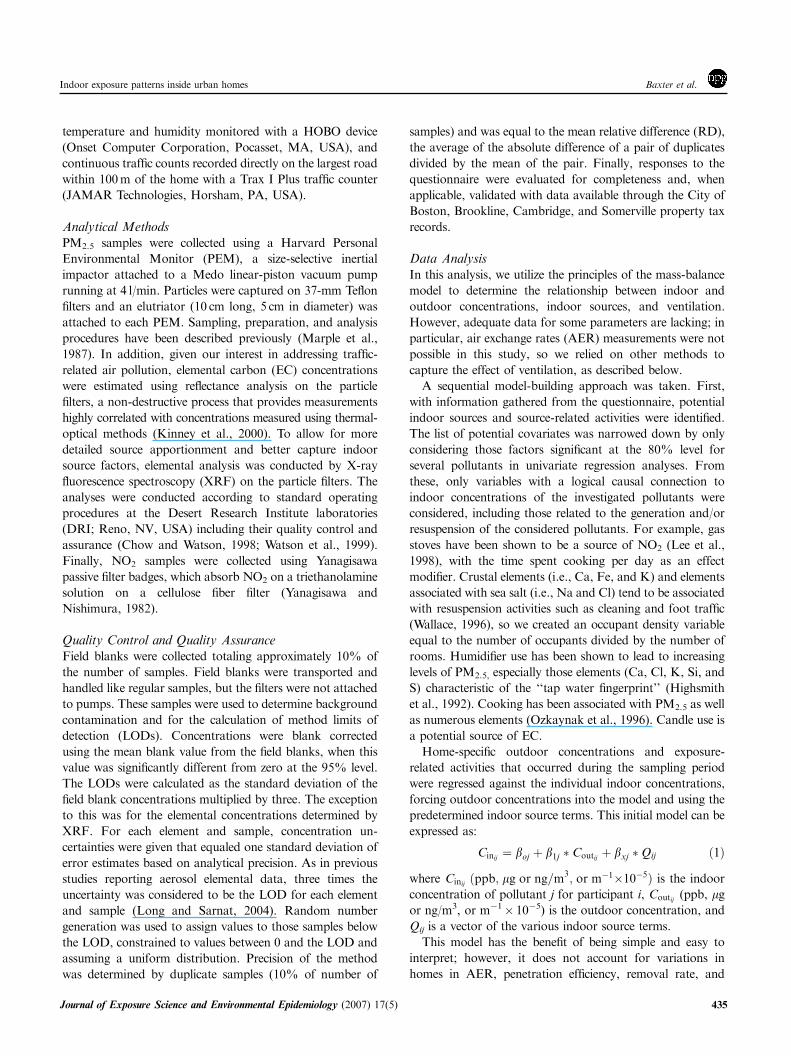
summarized in Table 1. The age and type of home are similar

in both cohort and non-cohort members. The non-cohort

members have slightly larger apartments, but the mean size

(less than five rooms) remains relatively small.

Household activities identified as possible indoor sources

are presented in Table 2, along with their distributions and

our determination of which were considered as a possible

predictor for NO2, PM2.5 and selected particle constituents.

For the hypothesized sources of interest, such as cooking and

cleaning activities, there is adequate heterogeneity within the

study population in the frequency of these activities.

Indoor and Outdoor ConcentrationsThe percentage of samples above the LOD for each pollutant

is shown in Figure 2, with only those with at least 70% of the

Table 1. Distributions of basic home characteristics for all partici-pants, cohort members, and non-cohort members.

Categorical variables Total (n¼ 43)

(%)

Cohort

members

(n¼ 25) (%)

Non-cohort

members

(n¼ 18) (%)

Type of housing

Single-family home 5 4 6

Multi-family home 56 60 50

Apartment building 39 36 44

Year built

Before 1900 20 16 27

1900–1949 56 52 61

1950–1969 12 16 6

1970–later 12 16 6

Continuous variable Mean (SD) Mean (SD) Mean (SD)

Number of rooms 4.2 (1.7) 3.7 (1.2) 4.8 (2.1)

Table 2. Distributions of selected household activities for all sampling sessions.

Categorical variables Percent (%) Potential source term for

Cleaning activitiesa (n¼ 61) PM2.5, Ca, Fe, K , Si, Na, Cl, Zn

0–1 activity/week 33

2–3 activities/week 67

Humidifier use (n¼ 61) PM2.5, Ca, K, Si, Cl

No 82

Yes 18

Candle use (n¼ 61) PM2.5, EC

No 74

Yes 26

Cooking time (n¼ 61) PM2.5, EC, Ca, Fe, K, Si, Na, Cl, Zn

r1 h/day 66

41 h/day 34

Gas stove usage (n¼ 59) (stove type*cooking time/day) NO2

Electric*r1 h/day, Electric*41 h/day, and Gas*r1 h/day 75

Gas*41 h/day 25

Continuous variables Mean (SD)

Occupant density (n¼ 61) (number of occupants/rooms) 0.99 (0.58) PM2.5, Ca, Fe, K, Si, Na, Cl, Zn

aCleaning, sweeping, and/or vacuuming.

Figure 2. Percentage of samples above the LOD. (LOD’s for NO2,PM2.5, and EC based on method blank values, all others are based onuncertainty limits).

Indoor exposure patterns inside urban homes Baxter et al.

Journal of Exposure Science and Environmental Epidemiology (2007) 17(5) 437

samples above the LOD included in formal regression

analyses. With the exception of NO2 (32%) and Cl (40%),

the mean RD was less than 25% for all pollutants, indicating

reasonable method precision.

Summary statistics for the measured residential indoor

and outdoor concentrations and I/O ratios are presented

in Table 3. All pollutant concentrations appear to be

lognormally distributed, as shown by Shapiro–Wilks tests

on the log-transformed data (a¼ 0.05), with concentrations

both indoors and outdoors spanning an order of magnitude.

Median I/O ratios are significantly greater than 1 for PM2.5,

Ca, and Cl as determined by a one sample median test

(Po0.05). I/O ratios for Fe, Zn, S, and V are significantly

less than 1 (Po0.05), with the I/O ratio for EC being

marginally significantly less than 1 (Po0.1). For NO2, K,

and Si, I/O ratios are not significantly different than 1,

although they varied significantly across sites.

Results from the regression analyses of outdoor concen-

trations against indoor concentrations are shown in Table 4.

Outliers were removed that unduly influenced regression

results, defined as having an absolute studentized residual

greater than four. The b1s are the coefficients of the outdoor

term in Equation (1), without consideration of indoor source

terms. Outdoor pollutant concentrations explained between

78% (S) and 7% (NO2) of the variability seen in indoor

concentrations (excluding Si), and the outdoor term was

significant (Po0.1) for all pollutants except Si. As antici-

pated, the coefficients (b1s) are generally higher for combus-

tion pollutants and lower for crustal elements, which are

larger and have lower penetration efficiencies.

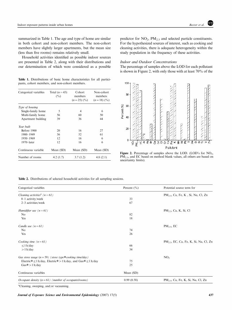
Identification of Indoor Source TermsRegression analyses were performed according to the model

described by Equation (1), with the indoor concentrations

as the dependent variables and outdoor concentrations and

selected source terms as the independent variables. Variables

and regression coefficients are shown in Table 5. Cooking for

more than an hour per day (as compared to less than an

hour) was associated with a significant increase in PM2.5 and

Zn. Occupant density significantly predicted indoor PM2.5,

Na, Cl, and Si concentrations. Additionally, performing

more than one cleaning activity was negatively associated

with indoor Fe levels, and humidifier use was associated with

an increase in indoor Ca. Cooking on a gas stove for more

than an hour significantly increased indoor NO2 levels, as

compared to cooking for less than an hour or on an electric

stove. Of note, no source terms were associated with indoor

V, but humidifier use was associated with indoor S. However,

this term was actually associated with a decrease in indoor

levels, and before the addition of any source terms, the

intercept was statistically insignificantly different from zero

for S. In addition, few homes demonstrated indoor/outdoor

ratios of sulfur significantly greater than 1, with only four of

56 ratios above 1.05. Thus, this does not provide significant

evidence of indoor sources of S in this cohort. Outdoor

Table 3. Indoor and outdoor residential pollutant concentrations and I/O ratios.

Outdoor concentrations Indoor concentrations Indoor/outdoor ratios

Pollutant N Median Mean (SD) Range N Median Mean (SD) Range N Median (CV)

NO2 (ppb) 52 16.8 17.2 (5.67) 5.21–33.3 54 17.1 19.6 (11.0) 5.67–61.1 51 0.99 (0.63)

PM2.5 (mg/m3) 60 12.6 14.2 (5.43) 6.75–31.3 64 16.7 20.3 (12.5) 6.77–74.9 58 1.14 (0.71)

EC (m�1� 10�5) 58 0.55 0.63 (0.49) 0.08–3.8 62 0.49 0.57 (0.35) 0.12–2.2 56 0.89 (0.64)

Ca (ng/m3) 58 24.4 29.4 (17.2) 9.12–113 62 32.1 48.0 (84.8) 12.8–676 56 1.16 (1.90)

Fe (ng/m3) 58 61.7 66.5 (26.4) 15.4–162 62 44.5 46.1 (20.0) 3.50–101 56 0.69 (0.40)

K (ng/m3) 58 46.8 57.5 (56.7) 19.1–446 62 82.2 78.6 (8.22) 15.2–477 56 1.10 (0.95)

Si (ng/m3) 58 34.9 55.9 (71.9) 4.81–467 62 38.3 83.4 (200) 5.53–1480 56 1.04 (1.31)

Na (ng/m3) 58 119 144 (160) 29.2–1260 62 128 185 (320) 2.27–2520 56 1.05 (1.84)

Cl (ng/m3) 58 4.25 15.2 (41.4) 0.194–3050 62 20.8 87.2 (3680) 0.528–2920 56 3.18 (3.79)

Zn (ng/m3) 58 10.9 14.7 (19.3) 5.23–1520 62 8.86 14.7 (18.0) 3.40–1050 56 0.83 (1.13)

S (ng/m3) 58 1280 1540 (1450) 413–11300 62 928 1120 (699) 310–3910 56 0.76 (0.32)

V (ng/m3) 58 3.52 4.79 (4.00) 1.08–22.5 62 2.84 3.54 (2.66) 0.392–15.5 56 0.76 (0.46)

Table 4. Univariate regression analysis of outdoor concentrations on

indoor concentrations.

Pollutant b1 (SE) P-value R2

NO2 0.48 (0.26) 0.07 0.07

PM2.5 0.91 (0.23) 0.01 0.23

EC 0.72 (0.10) o0.0001 0.49

Ca 0.56 (0.12) 0.01 0.30

Fe 0.38 (0.09) o0.0001 0.26

K 0.83 (0.11) o0.0001 0.52

Si 0.02 (0.07) 0.78 0.00

Na 0.46 (0.07) o0.0001 0.43

Cl 0.40 (0.15) 0.01 0.12

Zn 0.85 (0.19) o0.0001 0.28

S 0.95 (0.07) o0.0001 0.78

V 0.60 (0.04) o0.0001 0.77

Indoor exposure patterns inside urban homesBaxter et al.

438 Journal of Exposure Science and Environmental Epidemiology (2007) 17(5)

concentrations remained significant for all pollutants but Si.

To note, all regression analyses were repeated using a

stepwise selection approach and the results were unchanged.

Effect Modification by Air Exchange RatesThe I/O ratio of sulfur was dichotomized at the median

(0.76) to serve as a proxy for ‘high’ and ‘low’ AERs and was

only included as an effect modifier of outdoor concentrations

without modifying the effect of indoor sources (Table 6), due

to the limited statistical power and resulting statistical

instability when effect modification of indoor sources was

included. The effect estimates for the indoor source terms

remained similar in magnitude and significance after the

addition of the interaction terms. The exception was in the

indoor Fe model where the effect estimate for the cleaning

activities term was still negative, but smaller in magnitude

(�3 ng/m3) and no longer significant. For the pollutants

without identified indoor sources, with the exception of K,

there was generally a larger effect of outdoor concentrations

in homes in the high AER category compared with homes in

the low AER category, as anticipated. However, the

interaction term was only significant for S and V. For most

Table 5. Identification of indoor source terms contributing to indoor concentrations after adjusting for outdoor concentrations.a

Outdoor

concentration

Cooking time

(r1h/day¼ 0,

41h/day¼ 1)

Candle use

(No¼ 0,

Yes¼ 1)

Humidifier use

(No¼ 0,

Yes¼ 1)

Cleaning activities

(r1/week¼ 0,

41/week¼ 1)

Occupant

density

Gas stove usage

(otherb¼ 0,

gas*41 h/day ¼ 1)

Pollutant R2 Estimate (SE) Estimate (SE) Estimate (SE) Estimate (SE) Estimate (SE) Estimate (SE) Estimate (SE)

NO2 (ppb) 0.16 0.531 (0.224)** N/Ac N/A N/A N/A N/A 5.70 (3.06)*

PM2.5 (mg/m3) 0.37 0.878 (0.225)** 5.71 (2.92)** �2.46 (3.17) �1.34 (3.17) �0.364 (2.78) 4.11 (2.55)* N/A

EC (m�1� 10 �5) 0.52 0.738 (0.111)** �0.054 (0.056) 0.012 (0.068) N/A N/A N/A N/A

Ca (ng/m3) 0.48 0.446 (0.117)** �4.27 (4.67) N/A 15.2 (5.72)** 3.28 (4.34) 4.19 (3.91) N/A

Fe (ng/m3) 0.30 0.391 (0.093)** 0.950 (5.53) N/A N/A �9.95 (5.15)** 8.14 (4.38) N/A

K (ng/m3) 0.54 0.817 (0.117)** 10.3 (15.7) N/A 19.1 (19.0) 11.8 (14.8) �14.7 (13.2) N/A

Si (ng/m3) 0.05 0.020 (0.070) �5.38 (12.3) N/A �13.3 (15.2) �3.62 (11.0) 15.4 (10.1)* N/A

Na (ng/m3) 0.47 0.452 (0.075)** 17.1 (28.9) N/A N/A �16.0 (26.4) 30.5 (22.5)* N/A

Cl (ng/m3) 0.24 0.227 (0.168)* 5.46 (15.4) N/A �3.17 (19.30) 12.3 (13.9) 27.0 (12.9)** N/A

Zn (ng/m3) 0.36 0.813 (0.211)** 5.82 (2.61)** N/A N/A �1.18 (2.44) 0.694 (2.22) N/A

S (ng/m3) 0.80 0.951 (0.070)** N/A N/A �214.5 (114.3)** N/A N/A N/A

V (ng/m3) 0.77 0.596 (0.044)** N/A N/A N/A N/A N/A N/A

a**Po0.1 and *Po0.2.bIncludes all homes with electric stoves and those with gas stoves and cooking time of r1 h per day.cN/A: variable not considered a potential covariate for the pollutants.

Table 6. Effects of outdoor concentrations on indoor concentrations modified by I/O sulfur category.a

High I/O S Low I/O S

Pollutant R2 Estimate (SE) P-value Estimate (SE) P-value Significance of interaction termb

Pollutants without indoor sources

EC (m�1� 10�5) 0.50 0.791 (0.121) o0.0001 0.705 (0.103) o0.0001 NS

K (ng/m3) 0.52 0.834 (0.111) o0.0001 0.963 (0.287) o0.01 NS

S (ng/m3) 0.93 1.00 (0.040) o0.0001 0.641 (0.050) o0.0001 **

V(ng/m3) 0.79 0.754 (0.085) o0.0001 0.596 (0.043) o0.0001 **

Pollutants with indoor sources

NO2 (ppb) 0.16 0.557 (0.235) 0.03 0.473 (0.250) 0.07 NS

PM2.5 (mg/m3) 0.35 0.898 (0.230) o0.001 0.781 (0.254) o0.01 NS

Ca (ng/m3) 0.46 0.557 (0.133) o0.001 0.439 (0.125) 0.001 NS

Fe (ng/m3) 0.39 0.543 (0.100) o0.0001 0.347 (0.086) o0.001 **

Si (ng/m3) 0.06 0.118 (0.104) 0.26 �0.010 (0.077) 0.90 NS

Na (ng/m3) 0.46 0.493 (0.184) 0.01 0.442 (0.074) o0.0001 NS

Cl (ng/m3) 0.29 1.16 (0.460) 0.02 0.139 (0.157) 0.38 **

Zn (ng/m3) 0.38 0.659 (0.223) o0.001 0.877 (0.190) o0.0001 *

aFinal models after backwards elimination model, effect estimates of indoor sources not shownbNS¼ not significant, **Po0.1 and *Po0.2.

Indoor exposure patterns inside urban homes Baxter et al.

Journal of Exposure Science and Environmental Epidemiology (2007) 17(5) 439

of the pollutants with identified indoor sources, a larger effect

of outdoor concentrations was observed in homes with high

AERs compared with homes with low AERs, with the

difference in effects significant for Fe and Cl. The exception is

for Zn where the effect appeared significantly larger in homes

with low AERs (albeit in a model excluding an interaction

term on indoor sources). For Si outdoor concentrations did

not have a significant effect on indoor concentrations for

homes in either AER category.

Influence of Home Vs. Participant CharacteristicsAlthough basic home characteristics are similar between

cohort and non-cohort members (Table 1), multiple activity

patterns differed significantly (Table 7). Cohort members

tended to cook and clean more, had more frequent air

conditioning use, less opening of windows, and greater

occupant density. Thus, a comparison between these groups

can provide another means to determine the influence of

occupant activity patterns on I/O ratios.

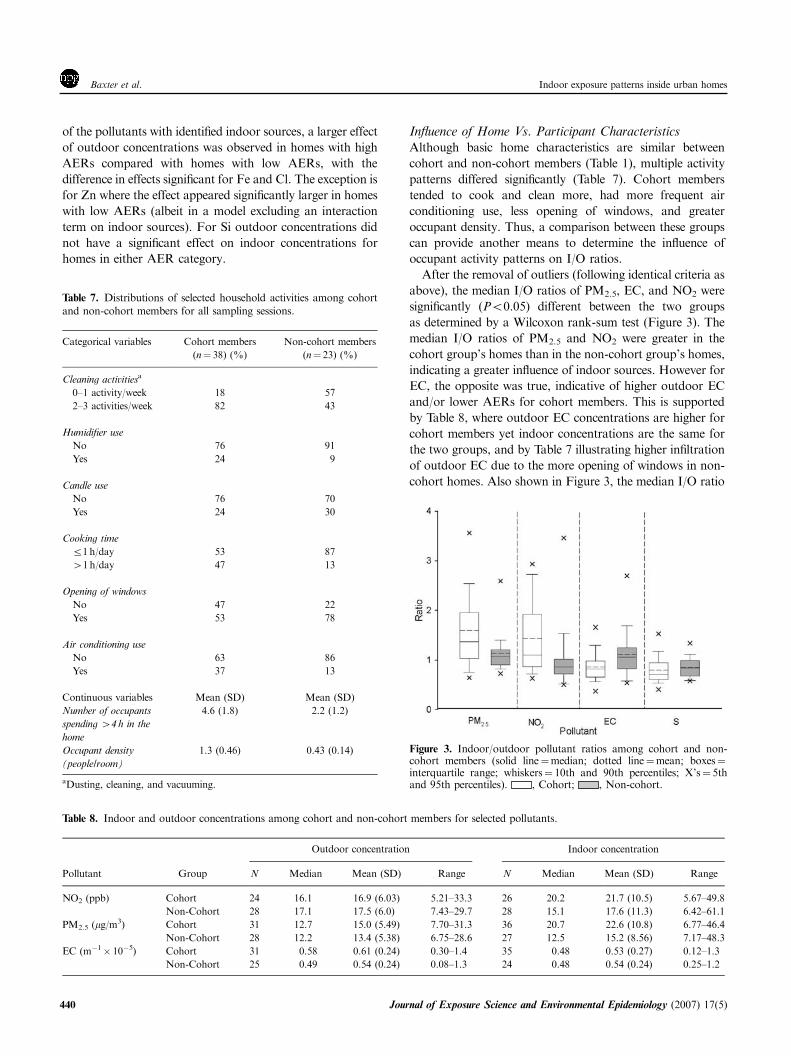
After the removal of outliers (following identical criteria as

above), the median I/O ratios of PM2.5, EC, and NO2 were

significantly (Po0.05) different between the two groups

as determined by a Wilcoxon rank-sum test (Figure 3). The

median I/O ratios of PM2.5 and NO2 were greater in the

cohort group’s homes than in the non-cohort group’s homes,

indicating a greater influence of indoor sources. However for

EC, the opposite was true, indicative of higher outdoor EC

and/or lower AERs for cohort members. This is supported

by Table 8, where outdoor EC concentrations are higher for

cohort members yet indoor concentrations are the same for

the two groups, and by Table 7 illustrating higher infiltration

of outdoor EC due to the more opening of windows in non-

cohort homes. Also shown in Figure 3, the median I/O ratio

Table 7. Distributions of selected household activities among cohortand non-cohort members for all sampling sessions.

Categorical variables Cohort members

(n¼ 38) (%)

Non-cohort members

(n¼ 23) (%)

Cleaning activitiesa

0–1 activity/week 18 57

2–3 activities/week 82 43

Humidifier use

No 76 91

Yes 24 9

Candle use

No 76 70

Yes 24 30

Cooking time

r1 h/day 53 87

41 h/day 47 13

Opening of windows

No 47 22

Yes 53 78

Air conditioning use

No 63 86

Yes 37 13

Continuous variables Mean (SD) Mean (SD)

Number of occupants

spending 44 h in the

home

4.6 (1.8) 2.2 (1.2)

Occupant density

(people/room)

1.3 (0.46) 0.43 (0.14)

aDusting, cleaning, and vacuuming.

Figure 3. Indoor/outdoor pollutant ratios among cohort and non-cohort members (solid line¼median; dotted line¼mean; boxes¼interquartile range; whiskers¼ 10th and 90th percentiles; X’s¼ 5thand 95th percentiles). , Cohort; , Non-cohort.

Table 8. Indoor and outdoor concentrations among cohort and non-cohort members for selected pollutants.

Outdoor concentration Indoor concentration

Pollutant Group N Median Mean (SD) Range N Median Mean (SD) Range

NO2 (ppb) Cohort 24 16.1 16.9 (6.03) 5.21–33.3 26 20.2 21.7 (10.5) 5.67–49.8

Non-Cohort 28 17.1 17.5 (6.0) 7.43–29.7 28 15.1 17.6 (11.3) 6.42–61.1

PM2.5 (mg/m3) Cohort 31 12.7 15.0 (5.49) 7.70–31.3 36 20.7 22.6 (10.8) 6.77–46.4

Non-Cohort 28 12.2 13.4 (5.38) 6.75–28.6 27 12.5 15.2 (8.56) 7.17–48.3

EC (m�1� 10�5) Cohort 31 0.58 0.61 (0.24) 0.30–1.4 35 0.48 0.53 (0.27) 0.12–1.3

Non-Cohort 25 0.49 0.54 (0.24) 0.08–1.3 24 0.48 0.54 (0.24) 0.25–1.2

Indoor exposure patterns inside urban homesBaxter et al.

440 Journal of Exposure Science and Environmental Epidemiology (2007) 17(5)

of S appears to follow a similar pattern as EC with a higher

median for non-cohort members compared to cohort

members. Although not statistically significant (P¼ 0.2),

this suggests that infiltration rates and therefore AERs are

higher in homes of non-cohort members than of cohort

members, and that there is a greater influence of indoor

sources of EC (not identified in the regression analyses) in

non-cohort homes.

Discussion

Ambient and Non-ambient Contributions to IndoorConcentrationsIn our study, predicting 1-week average indoor concentra-

tions based solely on outdoor concentrations did not explain

the majority of the variability in many cases, reflecting the

influence of home-to-home variations in indoor sources,

occupant behaviors, and AERs. For NO2 and most particle

constituents (with the exception of outdoor-dominated

constituents like sulfur and vanadium), the addition of

selected indoor source terms improved the model’s predictive

power, significantly so in many cases (i.e., NO2, PM2.5, Ca,

Cl). Cooking time, gas stove usage, occupant density, and

humidifiers were identified as important contributors to

indoor levels. We also found additional information value

in a dummy variable created from indoor/outdoor ratios of

sulfur (AERDummyi), which theoretically captured AERs

and allowed us to better incorporate some of the principles of

the mass balance model.

Our measured residential indoor and outdoor concentra-

tions, and I/O relationships are largely comparable to those

seen in other studies (Zipprich et al., 2002; Brunekreef et al.,

2005; Meng et al., 2005). Our findings are also in general

agreement with present day models for predicting the impact

of indoor sources based on integrated measurements, which

identified gas appliances and cooking as important sources

of NO2 (Linaker et al., 1996; Levy et al., 1998; Rotko et al.,

2001; Garcia-Algar et al., 2004) and PM (Ozkaynak et al.,

1994; Brunekreef et al., 2005), respectively. The current

study also identified resuspension activities as affecting PM

exposure. These activities, often treated as episodic events

increasing short-term indoor particle concentrations,

(Thatcher and Layton, 1995; Abt et al., 2000; Long et al.,

2000) in our study seemed to also affect longer-term indoor

levels. The additional significance of resuspension factors in

our study may be associated with the smaller volumes and

greater crowding (higher occupant densities) among our

participants, as opposed to the single-family homes generally

sampled in other studies.

PTEAM estimated that cooking caused an average

increase of 9mg/m3 (Ozkaynak et al., 1996) in indoor PM2.5,

with EXPOLIS observing a 11.65 mg/m3 (Amsterdam)

cooking effect on PM2.5 (Brunekreef et al., 2005). Although

the differences in source covariates and averaging times

impair direct interpretability, our cooking time covariate in

Table 5 contributed a similar magnitude concentration

increase to PM2.5 as in the studies above (with a 5.7 mg/m3

increment associated with cooking more than 1 h/day).

Furthermore, our gas stove usage covariate in Table 5

contributed a similar magnitude increase (5.7 ppb) of NO2 as

in previous studies, where gas stove usage contributed

approximately 10–20 ppb to indoor concentrations (Lee

et al., 1998) and personal NO2 exposure were found to be

14 ppb higher in homes with gas stoves compared to those

without them (Levy et al., 1998). Of note, our study did not

examine ETS, as smoking (1–4 cigarettes/day) inside the

home was reported only during four sampling sessions. The

results did not change with the exclusion of these partici-

pants; therefore they remained in the final models.

Two exceptions to our agreement with the literature are for

NO2 and Si, where outdoor concentrations explain indoor

concentrations to a lesser extent than expected. For NO2,

there is evidence to suggest that inadequate statistical power

and measurement error may be a cause. Due to an error in

the laboratory, some samples taken during the heating season

were lost, resulting in a smaller sample size and an

unbalanced data set by season. Moreover, the mean RD

was 32% (as compared with 9% for PM2.5 and 12% for

EC), indicating poorer precision potentially affecting the

observed relationships. For Si, outdoor concentration was

not a statistically significant contributor to indoor concentra-

tions. One reason could be that the Si particles found

outdoors are too large to readily penetrate the building

envelope and/or have a short residence time so that they

deposit quickly once entering the indoor environment. This

rationale explains the weaker association for many other

crustal elements as well.

While we were able to capture some significant indoor

source terms, it is possible that they do not reflect direct

causal influences on concentrations, and some covariates

are somewhat difficult to interpret. For example, there are

numerous types of cooking activities that may have

differential effects on concentrations, and we were unable

to incorporate all potential covariates due to limited

statistical power. Additionally, some of the source terms

are correlated with one another and may be proxies for

multiple factors. For example, occupant density may not

only represent resuspension activities (more people moving

around causing more resuspension), but may also be

associated with SES and related occupant activity patterns.

In univariate regressions (results not shown), higher occupant

densities were significantly (Po0.05) associated with in-

creased cooking and cleaning, indicating the difficulty in

separating these source terms. Due to substantial differences

in occupant density by cohort status, occupant density was

also correlated with ventilation-related behaviors, further

complicating interpretation of this term. While factor

Indoor exposure patterns inside urban homes Baxter et al.

Journal of Exposure Science and Environmental Epidemiology (2007) 17(5) 441

analytic methods on questionnaire data could have resolved

some of the collinearity issues, this would have impaired

general interpretability and not resolved correlations between

source terms and non-source factors.

As we did not find evidence of significant indoor sources

of sulfur (all homes using humidifiers had lower AERs,

potentially explaining the negative relationship in Table 5)

and found a strong relationship between indoor and outdoor

concentrations (R2¼ 0.78), this dummy variable should

appropriately capture categories of AERs. Although not

statistically significant for some of the outdoor dominated

pollutants, there appears to be a trend with the coefficient

for outdoor concentrations increasing with increasing AER

category, indicating as expected that outdoor concentrations

are greater contributors to indoor concentrations at higher

AERs. The exception is for K where a larger effect estimate is

seen in homes with low AERs, although this difference is

insignificant. The reason for this result is unclear; one

possibility is that this model did not take into account the

effect on indoor sources. Although none were identified in the

primary analysis, this does not ensure that there are no

indoor sources of K.

For those pollutants with identified indoor sources, the

AER proxy demonstrated similar results to those of the

outdoor-dominated pollutants, with the exception of Zn

where there was a larger effect of outdoor concentrations

in the low AER category, although this difference was only

marginally significant (P¼ 0.19), This unexpected results

may possibly be due to the exclusion of an interaction

between AER and indoor source terms. Ideally, regression

models would incorporate this factor, but statistical power

was limited in this investigation and the resulting models

displayed significant instability. In addition to inadequate

statistical power, there were correlations between some of the

indoor source terms and FINF, such as occupant density,

which was negatively associated with the dichotomized I/O

sulfur ratios. More generally, significant measurement error

would also be anticipated using the effect modification on our

questionnaire responses. These data are proxies rather than

direct measurements of the indoor source strength, and in

accordance with the mass balance model, other factors such

as home volume may also have affected the relationships.

Even with the incorporation of ventilation characteristics,

the predictive power for most of the pollutants with indoor

sources was still relatively low, with less than half of the

variability explained in many cases. This raises questions

about the measurement error associated with using these

models in order to estimate long-term exposures for a cohort

study. However, in spite of the limitations, our models do

however identify which indoor sources appear to be

important, which both informs epidemiological investigations

and offers guidance for future design of questionnaires in

an epidemiological context. For example, more resolved

information on the frequency and duration of cooking

(including specific types of cooking) or humidifier use could

improve the effectiveness of the models. While these issues

were incorporated into our questionnaires, the categories

may have been too coarse to capture relatively small

gradients in exposure. In addition, many epidemiological

studies wish to classify people into exposure categories as

opposed to predicting the exact concentrations, and our

models may prove effective in this regard. More generally,

imperfect models addressing indoor exposures may reduce

exposure misclassification more than models that only

consider outdoor concentrations. Future analysis will focus

on evaluating the implication of any exposure misclassifica-

tion with our models or alternative approaches on epide-

miological studies.

Building Vs. Occupant CharacteristicsOne of the important dimensions of our study is the fact that

we recruited two distinct populations with similar basic

housing characteristics in similar neighborhoods, allowing

us to understand the influence of building vs. occupant

characteristics on indoor exposures. Their different activity

patterns resulted in more heterogeneity in their exposures due

solely to indoor sources. The cohort, consisting of pregnant

or recently pregnant women, spent much more time at home

(mean¼ 19.5 h/day) than the non-cohort members (mean-

10 h/day). Therefore, as suggested by Table 7, cohort

members may perform more activities generating indoor air

pollution, making their levels higher than those seen outdoors

or in non-cohort participant homes. There may also be a

difference in AERs, with homes in the cohort having lower

AERs than non-cohort homes. This suggests a difference in

housing characteristics or activity patterns that is not

captured by Table 1.

As we used convenience sampling methods to recruit

additional participants, largely focused on increased repre-

sentation of undersampled neighborhoods, it could be argued

that our findings may be less representative of the larger

cohort population by the inclusion of participants outside the

ACCESS cohort. Yet, these non-cohort homes were located

in the target neighborhoods and had similar basic housing

characteristics. More generally, in well-developed urban

areas there may be limited new residential construction, so

basic housing characteristics may be more homogeneous.

LimitationsAs in any monitoring study, this study was potentially limited

by errors in exposure measurements and methods of data

collection. The measurements collected during the sampling

period may not accurately represent typical conditions, limiting

our ability to draw broad conclusions about long-term

exposure patterns. In addition, in order to limit the effect of

our study on the subject’s activities, the sampling equipment

was placed out of the way and did not require any maintenance

by the participant. Thus, the time–activity patterns of the

Indoor exposure patterns inside urban homesBaxter et al.

442 Journal of Exposure Science and Environmental Epidemiology (2007) 17(5)

individual should not have been altered due to the burden of

the sampling equipment, although this meant our sampling

captured a region of the house instead of the participant’s (or

their child’s) personal exposures. However, the time–activity

data indicate that residential concentrations may be a reason-

able proxy for personal exposures of cohort members.

The housing characteristics and occupant activities used

depended on questionnaire data, and although a standar-

dized questionnaire was used, there may still be a lack of

accuracy and reliability in the data. Further, although

sampling was conducted in two different seasons (a heating

and non-heating season), these were broadly defined and

covered a period up to 6 months. Under ideal circumstances,

data collection would have occurred simultaneously across

all homes in each season to minimize seasonal variability, but

this was not logistically feasible. Therefore, each sampling

session was treated as an independent measurement.

In addition, the sample size limited our ability to explore a

larger range of potential indoor source terms. More variations

in indoor concentrations may have been accounted for by

including continuous variables for AERs or in more closely

adhering to a mass-balance model. Since AER was estimated

via a proxy (I/O of sulfur), using a continuous AER would

have required explicit assumptions about P and k, and we had

less confidence in these estimates than in creating broad

categories representing ‘high’ and ‘low’ AERs.

Conclusions

In conclusion, the current paper identified important

predictors of indoor concentrations for multiple air pollutants

in a low SES urban population, including outdoor concen-

trations, indoor source terms, and proxies for AERs. This

allows us to determine the information necessary to assess

long-term indoor exposures. The important indoor sources

include average cooking time per day, humidifier use,

occupant density, and gas stove usage, with different sources

important for different pollutants, indicating that the

questionnaire data needed will be dictated by the pollutant

being studied. The crustal and sea salt elements were mainly

associated with occupant density, with aggregate PM2.5 also

associated with cooking time, and indoor NO2 increasing

with increasing gas stove usage. We also found it useful to

capture AERs in a context where AERs could not be

measured by dichotomizing the I/O ratios of sulfur, although

this covariate was more informative for outdoor source

dominated pollutants. Additionally, our cohort vs. non-

cohort analysis illustrated that it was the occupant activity

patterns that were driving the indoor exposure patterns rather

than the basic housing characteristics.

In general, our study provides some direction regarding

how exposure-related questionnaires should be refined in

population studies, in order to predict indoor exposures in

the absence of measurements, which are often not possible

for a large cohort. We have demonstrated that, in lower-SES

urban dwellings (largely multi-unit), resuspension activities

along with cooking and stove usage appear to contribute

significantly to longer-term indoor exposures to some

pollutants. The importance of resuspension activities has

not been observed in studies focusing on single-family homes,

indicating that more research is needed in urban areas where

more people reside in multi-unit dwellings with higher

occupant densities. Incorporating this information will lead

to more accurate predictions of indoor pollutant levels for

lower SES populations, improving our ability to detect health

effects in large cohort studies. Future studies will consider the

information value of GIS and other publicly available data in

predicting indoor exposure patterns in the absence of outdoor

monitoring and detailed activity information, which are often

difficult to obtain in these types of studies.

Acknowledgements

This research was supported by HEI 4727-RFA04-5/05-1,

NIH U01 HL072494, NIH R03 ES013988, PHS 5-T42-

CCT1229661-02, and PHS 1-T42-OH008416-01. We grate-

fully acknowledge the hard work of all the technicians

associated with the ACCESS project and the hospitality of

the ACCESS and other study participants. In addition, we

thank Dr. Rosalind Wright of the Channing Laboratory,

Christopher Paciorek from the Department of Biostatistics at

Harvard School of Public Health, and Helen Suh from the

Department of Environmental Health at Harvard School

of Public Health for providing guidance; Prashant Dilwali,

Robin Dodson, Shakira Franco, Lu-wei Lee, Rebecca

Schildkret, and Leonard Zwack for their sampling assistance;

and Monique Perron for both her sampling and laboratory

assistance.

References

Abt E., Suh H.H., Allen G., and Koutrakis P. Characterization of indoor particle

sources: a study conducted in the metropolitan Boston area. Environ Health

Perspect 2000: 108(1): 35–44.

American Lung Association. Urban air pollution and health inequities: a

workshop report. Environ Health Perspect 2001: 109(Suppl 3): 357–374.

Brauer M., Hoek G., van Vliet P., Meliefste K., Fischer P., Gehring U., Heinrich

J., Cyrys J., Bellander T., Lewne M., and Brunekreef B. Estimating long-term

average particulate air pollution concentrations: application of traffic

indicators and geographic information systems. Epidemiology 2003: 14(2):

228–239.

Breysse P.N., Buckley T.J., Williams D.A., Beck C.M., Jo S.-J., Merriman B.,

Kanchanaraksa S., Swartz L.J., Callahan K.A., and Butz A.M. Indoor

exposures to air pollutants and allergens in the homes of asthmatic children in

inner-city Baltimore. Environ Res 2005: 98(2): 167–176.

Briggs D.J., De Hoogh C., Gulliver J., Wills J., Elliott P., Kingham S., and

Smallbone K. A regression-based method for mapping traffic-related air

pollution: application and testing in four contrasting urban environments. Sci

Total Environ 2000: 253(1–3): 151–167.

Brunekreef B., Janssen N.A.H., De Hartog J.J., Oldenwening M., Meliefste K.,

Hoek G., Lanki T., Timonen K.L., Vallius M., Pekkanen J., and Van Grieken

Indoor exposure patterns inside urban homes Baxter et al.

Journal of Exposure Science and Environmental Epidemiology (2007) 17(5) 443

R. Personal, Indoor, and Outdoor Exposures to PM2.5 and its Components for

Groups of Cardiovascular Patients in Amsterdam and Helsinki 2005, Boston,

MA, Health Effects Institute.

Centers for Disease Control and Prevention. Use of unvented residential heating

appliancesFUnited States, 1988–1994. Morbidity Mortality Wkly Rep 1997:

46(51): 1221–1224.

Centers for Disease Control and Prevention. Cigarette smoking among adults –

United States, 2002. Morbidity Mortality Wkly Rep 2004: 53(20): 427–431.

Chow J., and Watson J. Guidelines on Speciated Particulate Monitoring, Third

Draft Report 1998, Research Triangle Park, NC, US. Environmental

Protection Agency, Office of Air Quality Planning and Standards.

Garcia-Algar O., Pichini S., Basagana X., Puig C., Vall O., Torrent M., Harris J.,

Sunyer J., and Cullinan P. Concentrations and determinants of NO2 in homes

of Ashford, UK and Barcelona and Menorca, Spain. Indoor Air 2004: 14(4):

298–304.

Highsmith V.R., Hardy R.J., Costa D.L., and Germani M.S. Physical and

chemical characterization of indoor aerosols resulting from the use of tap water

in portable home humidifiers. Environ Sci Technol 1992: 26(4): 673–680.

Kinney P.L., Aggarwal M., Northridge M.E., Janssen N.A.H., and Shepard P.

Airborne concentrations of PM2.5 and diesel exhaust particles on Harlem

sidewalks: a community-based pilot study. Environ Health Perspect 2000:

108(3): 213–218.

Koistinen K.J., Hanninen O., Rotko T., Edwards R.D., Moschandreas D., and

Jantunen M.J. Behavioral and environmental determinants of personal

exposures to PM2.5 in EXPOLIS – Helsinki, Finland. Atmos Environ 2001:

35(14): 2473–2481.

Kousa A., Monn C., Rotko T., Alm S., Oglesby L., and Jantunen M.J. Personal

exposures to NO2 in the EXPOLIS-study: relation to residential indoor,

outdoor, and workplace concentrations in Basel, Helsinki, and Prague. Atmos

Environ 2001: 35(20): 3405–3412.

Koutrakis P., and Briggs S.L.K. Source apportionment of indoor aerosols in

Suffolk and Onondage Counties, New York. Environ Sci Technol 1992: 26(3):

521–527.

Lee K., Levy J.I., Yanagisawa Y., and Spengler J.D. The Boston residential

nitrogen dioxide characterization study: classification of and prediction of on

indoor NO2 exposure. J Air Waste Manage Assoc 1998: 48(8): 739–742.

Lee K., Yang W., and Bofinger N.D. Impact of micorenvironmental nitrogen

dioxide concentrations on personal exposures in Australia. J Air Waste

Manage Assoc 2000: 50(10): 1739–1744.

Levy J.I., Lee K., Spengler J.D., and Yanagisawa Y. Impact of residential nitrogen

dioxide exposure on personal exposure: an international study. J Air Waste

Manage Assoc 1998: 48(6): 553–560.

Linaker C.H., Chauhan A.J., Inskip H., Frew A., Sillence A., Coggon D., and

Holgate S.T. Distribution and determinants of personal exposure to nitrogen

dioxide in school children. Occup Environ Med 1996: 53(3): 200–203.

Long C.M., and Sarnat J.A. Indoor–outdoor relationships and infiltration

behavior of elemental components of outdoor PM2.5 for Boston-area homes.

Aerosol Sci Technol 2004: 38(S2): 91–104.

Long C.M., Suh H.H., and Koutrakis P. Characterization of indoor particle

sources using continuous mass and size monitors. J Air Waste Manage Assoc

2000: 50(7): 1236–1250.

Marple V.A., Rubow K.L., Turner W., and Spengler J.D. Low flow rate sharp cut

impactors for indoor air sampling: design and calibration. J Air Pollut Control

Assoc 1987: 37(11): 1303–1307.

Meng Q.Y., Turpin B.J., Polidori A., Lee J.H., Weisel C.P., Morandi M., Colome

S., Stock T., Winer A., and Zhang J. PM2.5 of ambient origin: estimates and

exposure errors relevant to PM epidemiology. Environ Sci Technol 2005:

39(14): 5105–5112.

O’Neill M.S., Jerrett M., Kawachi I., Levy J.I., Cohen A.J., Gouveia N.,

Wilkinson P., Fletcher T., Cifuentes L., Schwartz J., and Conditions

W.o.A.P.a.S. Health, wealth, and air pollution: advancing theory and

methods. Environ Health Perspect 2003: 111(16): 1861–1870.

Ozkaynak H., Xue J., Spengler J., Wallace L., Pellizzari E., and Jenkins P.

Personal exposure to airborne particles and metals: results from the Particles

Team Study in Riverside, California. J Exp Anal EnviornEpidemiol 1996: 6(1):

57–78.

Ozkaynak H., Xue J., Weker R., Butler D., Koutrakis P., and Spengler J. The

Particle Team (PTEAM) Study: Analysis of the Data. Final Report. Vol. III

1994, Research Triangle Park, NC, US EPA.

Rotko T., Kousa A., Alm S., and Jantunen M. Exposures to nitrogen dioxide in

EXPOLIS – Helsinki: microenvironment, behavioral, and sociodemographic

factors. J Exp Anal Environ Epidemiol 2001: 11(3): 216–223.

Sarnat J.A., Long C.M., Koutrakis P., Coull B.A., Schwartz J., and Suh H.H.

Using sulfur as a tracer of outdoor fine particulate matter. Environ Sci Technol

2002: 36(24): 5305–5314.

Schwab M., McDermott A., Spengler J.D., Samet J.M., and Lambert W.E.

Seasonal and yearly patterns of indoor nitrogen dioxide levels: data from

Albuquerque, New Mexico. Indoor Air 1994: 4(1): 8–22.

Thatcher T.L., and Layton D.W. Deposition, resuspension, and penetration of

particles within a residence. Atmos Environ 1995: 29(13): 1487–1497.

The American Lung Association. Urban air pollution and health inequities: a

workshop report. Environ Health Perspect 2001: 109(Suppl 3): 357–374.

Wallace L.A. Indoor particles: a review. J Air Waste Manage Assoc 1996: 46(2):

98–126.

Wallace L.A., Mitchell H., O’Connor G.T., Neas L., Lippmann M., Kattan M.,

Koenig J., Stout J.W., Vaughn B.J., Wallace D., Walter M., Adams K., and

Liu L.S. Particle concentrations in inner-city homes, of children with asthma:

the effect of smoking, cooking, and outdoor pollution. Environ Health

Perspect 2003: 111(9): 1265–1272.

Watson J., Chow J., and Frazier C. X-ray fluorescence analysis of ambient air

samples. In: Landberger S. and Creatchman M. (Eds.). Elemental Analysis of

Airborne Particles. Gordon and Breach Publishers, NJ, 1999 pp. 67–96.

Williams R., Suggs J., Rea A., Leovic K., Vette A., Croghan C., Sheldon L.,

Rodes C., Thornburg J., Ejire A., Herbst M., and Sanders Jr W. The

Research Triangle Park particulate matter panel study: PM mass concentration

relationships. Atmos Environ 2003: 37(38): 5349–5363.

Yanagisawa Y., and Nishimura H. A badge-type personal sampler for

measurement of personal exposure to NO2 and NO in ambient air. Environ

Int 1982: 8(1–6): 235–242.

Zipprich J.L., Harris S.A., Fox C., and Borzelleca J.F. An analysis of factors that

influence personal exposure to nitrogen dioxides in residents of Richmond,

Virginia. J Exp Anal Environ Epidemiol 2002: 12(4): 273–285.

Indoor exposure patterns inside urban homesBaxter et al.

444 Journal of Exposure Science and Environmental Epidemiology (2007) 17(5)