Prediction with measurement errors in finite populations

Prediction with measurement errors in finite populations

Julio M Singer1, Edward J Stanek III2, Viviana B Lencina3,Luz Mery Gonzalez4, Wenjun Li5 and Silvina San Martino6

1Departamento de Estatıstica, Universidade de Sao Paulo, Brazil2Department of Public Health, University of Massachusetts at Amherst, USA

3Facultad de Ciencias Economicas, Universidad Nacional de Tucuman, CONICET, Argentina4Departamento de Estadıstica, Universidad Nacional de Colombia, Bogota, Colombia

5Division of Preventive and Behavioral Medicine, University of Massachusetts, Worcester, USA6Facultad de Ciencias Agrarias, Universidad Nacional de Mar del Plata, Argentina

Abstract

We address the problem of selecting the best linear unbiased predictor (BLUP) of thelatent value (e.g., serum glucose fasting level) of sample subjects with heteroskedastic mea-surement errors. Using a simple example, we compare the usual mixed model BLUP toa similar predictor based on a mixed model framed in a finite population (FPMM) setupwith two sources of variability, the first of which corresponds to simple random samplingand the second, to heteroskedastic measurement errors. Under this last approach, we showthat when measurement errors are subject-specific, the BLUP shrinkage constants are basedon a pooled measurement error variance as opposed to the individual ones generally consid-ered for the usual mixed model BLUP. In contrast, when the heteroskedastic measurementerrors are measurement condition-specific, the FPMM BLUP involves different shrinkageconstants. We also show that in this setup, when measurement errors are subject-specific,the usual mixed model predictor is biased but has a smaller mean squared error than theFPMM BLUP which point to some difficulties in the interpretation of such predictors.

Keywords: finite population, heteroskedasticity, superpopulation, unbiasedness.

1 Introduction

Mixed models have a long history in the statistical literature and have been used to an-

alyze data from many fields, like Agriculture, Genetics, Medicine etc. They are not only ex-

tremely flexible and useful to model the covariance structure of correlated data but also allow

both subject-specific and population-averaged analyses as indicated in Verbeke and Molenberghs

(2001), for example. The importance of mixed models is clearly demonstrated by the variety

of texts that have been recently published on the subject. Verbeke and Molenberghs (2001),

Diggle et al. (2002), Demidenko (2004), Fitzmaurice et al. (2008) are excellent examples.

1

The linear mixed model may be expressed as

Y = Xα + ZB + E (1)

where Y is an n× 1 response vector, X and Z are, respectively, n× p and n× q known model

specification matrices, α is a p × 1 vector of unknown parameters (fixed effects), B is a q × 1

vector of random elements (random effects) such that E(B) = 0 and V(B) = Γ, E is an n× 1

vector of random errors such that E(E) = 0 and V(E) = Σ and is not correlated with B. This

implies that

V(Y) = Ω = ZΓZ> + Σ. (2)

In many practical situations, we are interested not only in estimating α but also in predicting

B. The best linear unbiased estimator (BLUE) of α and the best linear unbiased predictor

(BLUP) of B are respectively given by

α = (X>Ω−1X)−1X>Ω−1Y

B = ΓZ>Ω−1(Y −Xα) (3)

which is the solution to the well-known Henderson equations [see Verbeke and Molenberghs

(2001), for example](X>Σ−1X X>Σ−1ZZ>Σ−1X Z>Σ−1Z + Γ−1

)(α

B

)=

(X>Σ−1YZ>Σ−1Y

). (4)

It follows that the BLUP of

Q = k>1 α + k>2 B (5)

where k1 and k2 are known p × 1 and q × 1 vectors is Q = k>1 α + k>2 B. Although many

derivations of these results are available, it is possible, as indicated in Harville (1990), to obtain

the BLUP assuming only the existence of the first and second moments as considered above.

An outline of this derivation is given in Appendix A. The reader is also referred to Robinson

(1991) for an excellent account on the subject.

Linear mixed models may be used to predict latent values in the presence of heteroskedastic

measurement errors, as seen in Stanek et al. (1999), for example. Specification of the appropriate

mixed model for such purposes may be tricky, as we show by the following example.

With the objective of evaluating the impact of physical activity on gestational diabetes,

suppose that a single measurement of fasting serum glucose (sg) level is made on each of n

2

pregnant women sampled from a hospital practice. Women with sufficiently elevated fasting

sg-levels are to be referred to a physician for further evaluation. The accuracy of the prediction

is important to ensure high sensitivity and specificity of the referrals. However, since fasting sg-

levels may vary from day to day, and the variance may differ among women, we plan to predict

latent fasting sg-levels for women in the sample appropriately accounting for this heterogeneous

subject-specific measurement variability.

A model usually employed for this problem is

Yi = µ+Bi + Ei, i = 1, . . . , n (6)

where Yi is the observed fasting sg-level for the i-th selected woman, µ is the population mean,

Bi, assumed to have null mean and variance γ2, represents the random effect of the i-th selected

woman and Ei, assumed to have null mean and variance σ2i , denotes the corresponding measure-

ment error; we also assume that Bi and Ei are uncorrelated. This model may be expressed as (1)

by letting X = 1n, where 1n denotes an n×1 vector with all elements equal to 1, α = µ, Z = In,

with In denoting the identity matrix of order n, B = (B1, . . . , Bn)>, Γ = γ2In and Σ = ⊕ni=1σ

2i

where ⊕ni=1σ

2i denotes an n× n diagonal matrix with the σ2i along the main diagonal, i.e,

Y = 1nµ+ InB + E. (7)

Under this setup, the BLUP for the latent fasting sg-level of the i-th selected woman, namely,

µ+Bi, which corresponds to (5) with k1 = 1 and k2 = ei where ei denotes an n× 1 vector with

a single nonnull element equal to 1 in the i-th position, may be obtained from (3) and simplifies

to

Yi = µ+ ki(Yi − µ) (8)

where µ =∑n

i=1(wi/∑n

i=1wi)Yi is a weighted mean with wi = (γ2+σ2i )−1 and ki = γ2/(γ2+σ2i )

is the corresponding shrinkage constant. Details are presented in Appendix A.

For simplicity, to see how the mixed model is used in the context of our finite population

example, suppose that a physician has N = 3 pregnant women in her practice and that we plan

to take a simple random sample of n = 2 women, and make a single measurement of fasting

sg-level on each woman. Normal fasting sg-levels are 4-8 mmoles/l; levels above 11.1 mmoles/l

indicate a diagnosis of diabetes. We assume that the population parameters (latent fasting

sg-levels and subject-specific measurement error variances) are those summarized in Table 1.

3

Table 1: Fasting serum glucose levels, subject-specific measurement error variances and shrinkageconstants for a population of 3 women

Subject Latent Measurement Shrinkagesg-level error variance constant

Daisy 10 1 0.950Lily 3 100 0.160Rose 2 4 0.826

Average µ = 5 σ2 = 35Variance γ2 = 19

We assume further that the variances are known and that the subject-specific measurement

error can take on only two possible equally likely values given by plus or minus the subject-

specific standard deviation. We wish to predict the latent fasting sg-level of each woman in the

sample and use the subject-specific variance components to define the shrinkage constants. The

observed response, Yi and the values of the predictor (8) are listed in Table 2 for all 24 possible

samples corresponding to the 4 possible combinations of response for each of the 6 possible

sample sequences. We also tabulate the squared difference between the value of each predictor

and the corresponding latent value; the averages over all samples are presented in the bottom

row.

The average value of predictor (8) is 5.8 and surprisingly it is not equal to the population

mean (5.0) although it was presumably derived under an unbiasedness assumption. Clearly, in

the setting where there is subject-specific measurement error, this predictor is not a BLUP since

the unbiasedness property does not hold. Our objective is to clarify such apparent inconsistency.

In Section 2 we discuss the nature of measurement errors and show that in this context, (8)

is a BLUP when measurement errors are heterogeneous, but not subject-specific. In Section 3,

we introduce a finite population mixed model that may be formulated as (1) but with a different

covariance structure depending on the nature of the measurement errors. We also show that for

heteroskedastic subject-specific measurement errors, the corresponding BLUP is not given by

(8). We conclude with a discussion in Section 4.

4

Table 2: Mixed model predictor (based on subject-specific measurement errors) of fasting latentsg-levels for selected women and squared errors for all possible samples

Woman Measurement Observed Predictor Squared(latent sg-level) error response∗ (8) error

Sample i = 1 i = 2 i = 1 i = 2 i = 1 i = 2 i = 1 i = 2 i = 1 i = 21 Daisy (10) Lily (3) 1 10 11 13 11.0 11.6 1.03 73.292 Daisy (10) Lily (3) 1 -10 11 -7 10.9 5.9 0.76 8.703 Daisy (10) Lily (3) -1 10 9 13 9.0 10.1 0.94 50.734 Daisy (10) Lily (3) -1 -10 9 -7 8.9 4.5 1.24 2.285 Daisy (10) Rose (2) 1 2 11 4 10.8 4.7 0.70 7.036 Daisy (10) Rose (2) 1 -2 11 0 10.7 1.0 0.55 0.957 Daisy (10) Rose (2) -1 2 9 4 8.9 4.5 1.25 6.088 Daisy (10) Rose (2) -1 -2 9 0 8.8 0.8 1.46 1.359 Lily (3) Daisy (10) 10 1 13 11 11.6 11.0 73.29 1.0310 Lily (3) Daisy (10) 10 -1 13 9 10.1 9.0 50.73 0.9411 Lily (3) Daisy (10) -10 1 -7 11 5.9 10.9 8.70 0.7612 Lily (3) Daisy (10) -10 -1 -7 9 4.5 8.9 2.28 1.2413 Lily (3) Rose (2) 10 2 13 4 6.7 4.3 13.41 5.0814 Lily (3) Rose (2) 10 -2 13 0 3.8 0.4 0.71 2.6715 Lily (3) Rose (2) -10 2 -7 4 0.7 3.7 5.08 2.8616 Lily (3) Rose (2) -10 -2 -7 0 -2.1 -0.2 25.71 4.8317 Rose (2) Daisy (10) 2 1 4 11 4.7 10.8 7.03 0.7018 Rose (2) Daisy (10) 2 -1 4 9 4.5 8.9 6.08 1.2519 Rose (2) Daisy (10) -2 1 0 11 1.0 10.7 0.95 0.5520 Rose (2) Daisy (10) -2 -1 0 9 0.8 8.8 1.35 1.4621 Rose (2) Lily (3) 2 10 4 13 4.3 6.7 5.08 13.4122 Rose (2) Lily (3) 2 -10 4 -7 3.7 0.7 2.86 5.0823 Rose (2) Lily (3) -2 10 0 13 0.4 3.8 2.67 0.7124 Rose (2) Lily (3) -2 -10 0 -7 -0.2 -2.1 4.83 25.71

Average 5.0 5.0 5.8 5.8 9.11 9.11

∗ Observed response = latent sg-level ± measurement error

2 Sources of measurement errors

In many situations, the actual measurement of a latent value is not possible because it may

be affected by many sources of variability. Such variability is termed measurement error by

Cochran (1977) or observation error by Sukhatme (1984). Measurement errors may arise in

different ways which can be classified into two types of sources. The first is subject-specific

and is associated to the natural variability of the response around a fixed value (the latent

value); it is called inherent variability by Buonaccorsi (2006). The second is associated with

the measurement process, i.e., measurement instruments or interviewers. With the same spirit

generally employed in the Econometric literature [see Kennedy (2008), for example], where

5

Table 3: Mixed model predictor (based on exogenous measurement errors) of fasting latentsg-levels for selected women and squared errors for all possible samples

Woman Measurement Observed Predictor Squared(latent sg-level) error response∗ (8) error

Sample i = 1 i = 2 i = 1 i = 2 i = 1 i = 2 i = 1 i = 2 i = 1 i = 21 Daisy (10) Lily (3) 1 2 11 5 10.9 5.6 0.74 6.542 Daisy (10) Lily (3) 1 -2 11 1 10.8 1.9 0.59 1.143 Daisy (10) Lily (3) -1 2 9 5 8.9 5.4 1.19 5.634 Daisy (10) Lily (3) -1 -2 9 1 8.8 1.7 1.41 1.585 Daisy (10) Rose (2) 1 2 11 4 10.8 4.7 0.70 7.036 Daisy (10) Rose (2) 1 -2 11 0 10.7 1.0 0.55 0.957 Daisy (10) Rose (2) -1 2 9 4 8.9 4.5 1.25 6.088 Daisy (10) Rose (2) -1 -2 9 0 8.8 0.8 1.46 1.359 Lily (3) Daisy (10) 1 2 4 12 4.2 11.3 1.41 1.5810 Lily (3) Daisy (10) 1 -2 4 8 4.1 7.6 1.19 5.6311 Lily (3) Daisy (10) -1 2 2 12 2.2 11.1 0.59 1.1412 Lily (3) Daisy (10) -1 -2 2 8 2.1 7.4 0.74 6.54

? 13 Lily (3) Rose (2) 1 2 4 4 4.0 4.0 1.00 4.0014 Lily (3) Rose (2) 1 -2 4 0 3.9 0.4 0.82 2.6515 Lily (3) Rose (2) -1 2 2 4 2.0 3.8 0.91 3.2916 Lily (3) Rose (2) -1 -2 2 0 2.0 0.2 1.10 3.2917 Rose (2) Daisy (10) 1 2 3 12 3.2 11.2 1.46 1.3518 Rose (2) Daisy (10) 1 -2 3 8 3.1 7.5 1.25 6.0819 Rose (2) Daisy (10) -1 2 1 12 1.3 11.0 0.55 0.9520 Rose (2) Daisy (10) -1 -2 1 8 1.2 7.3 0.70 7.0321 Rose (2) Lily (3) 1 2 3 5 3.0 4.8 1.10 3.2922 Rose (2) Lily (3) 1 -2 3 1 3.0 1.2 0.91 3.2923 Rose (2) Lily (3) -1 2 1 5 1.1 4.6 0.82 2.6524 Rose (2) Lily (3) -1 -2 1 1 1.0 1.0 1.00 4.00

Average 5.0 5.0 5.0 5.0 0.98 3.63

∗ Observed response = latent sg-level ± measurement error

variables may be classified as endogenous or exogenous, we refer to the first type of measurement

errors as endogenous measurement errors and the second, exogenous measurement errors. Using

this terminology, the measurement errors considered in Table 2 are endogenous.

Now suppose that in our example, the measurement errors are exogenous, i.e., related to

the measurement condition associated with the position (i = 1 or i = 2) in the sample, instead

of endogenous (subject-specific). Let us also assume that the exogenous measurement error

variance is 1 when i = 1 or 4 when i = 2 and for simplicity, that the measurement error may

take only two possible values, given by plus or minus the corresponding standard error. The

results are presented in Table 3.

6

Since the average value of predictor (8) is 5.0 (the true value), it is clearly unbiased and

the results indicate that the specification of the measurement errors in model (1) may help

in deciding whether (8) is or is not the BLUP and consequently in choosing the covariance

structure. Although we considered only a simple example, the conclusion holds in general as

shown in Appendix B.

To better understand this result, we follow the lines given in Stanek, Singer and Lencina

(2004) and Stanek and Singer (2004), and consider a finite population mixed model (FPMM)

that is directly connected to the physical problem it represents and show that it is useful in

identifying the appropriate model specification.

3 The finite population mixed model with measurement error

Let a population consist ofN labeled subjects and let the latent value for subject s correspond

to a fixed (but unknown) constant, ys. We assume that the potentially observable response for

subject s is Ys = ys + Ws and that it differs from the latent response ys by the endogenous

measurement error Ws. Defining µ = N−1∑N

s=1 ys, we express the latent value in terms of a

subject effect βs as

ys = µ+ βs. (9)

Adding endogenous measurement error to (9) we obtain the measurement error model for subject

s, namely

Ys = µ+ βs +Ws. (10)

We assume that ER(Ws) = 0 and ER(WsWs′) = σ2s for s = s′ and ER(WsWs′) = 0 other-

wise. The subscript R indicates expectation with respect to the distribution of the endogenous

measurement error. We also define γ2 = (N − 1)−1∑N

s=1(ys − µ)2.

To formalize the selection of a simple random sample (without replacement) we first represent

a permutation of subjects by a set of random variables, and assume that each permutation is

equally likely. Without loss of generality we may assume that the sample corresponds to the

set of the first n random variables in a permutation, with each random variable identified by its

position. Each of these is defined via a set of N indicator random variables Uis that take on a

value of one with probability 1/N if subject s is selected in position i, i = 1, . . . , N and zero

otherwise. For the response in position i, we specify the model that includes both sampling and

7

endogenous measurement error by

Y ∗i = µ+Bi +W ∗i (11)

where Y ∗i =∑N

s=1 UisYs, Bi =∑N

s=1 Uisβs and W ∗i =∑N

s=1 UisWs. The assumption that

sampling is without replacement implies that ES(UisUi′s′) = 0 if i = i′, s 6= s′ or i 6= i′, s = s′

but ES(UisUi′s′) = 1/[N(N − 1)] if i 6= i′, s 6= s′ where the subscript S indicates expectation

with respect to sampling. The random variables Y ∗i , i = 1, . . . , N, represent the permutations

of the N subjects in the population. The latent value for the subject selected in position i in a

sample is

Y +i =

N∑s=1

Uisys = µ+Bi i = 1, . . . , n. (12)

Although model (11) has the same form as model (6), it explicitly accounts for random

sampling with indicator random variables that underlie the definition of the random variables

Bi and W ∗i . When endogenous measurement error variances differ between subjects, the term

corresponding to Ei in (6), namely W ∗i , is such that

V(W ∗i ) = ES(N∑s=1

Uisσ2s) = N−1

N∑s=1

σ2s = σ2.

In other words, taking the expectation over sampling effectively averages the measurement error

variances over subjects in the population.

We can represent the FPMM for the sample as (7) with Y∗ = (Y ∗1 , . . . , Y∗n )> in lieu of Y

and W∗ = (W ∗1 , . . . ,W∗n)> in lieu of E. The variances of B and W∗ emerge directly from the

finite population mixed model development and are respectively given by Γ = γ2(In −N−1Jn)

where Jn = 11> and Σ = σ2In.

The corresponding BLUP for the latent fasting sg-level of the i-th selected woman, (12),

may be computed as in the mixed model setup and simplifies to

Y ∗i = Y∗

+ k(Y ∗i − Y∗) (13)

where Y∗

= n−1∑n

i=1 Y∗i is the sample mean and k = γ2/(γ2 + σ2). Details are given in

Appendix B.

The inclusion of the additional finite population term in the variance of B has no impact on

the expression for the predictor and even though the endogenous measurement error variances

8

Table 4: FPMM predictor (based on subject-specific measurement errors) of fasting latent sg-levels for selected women and squared errors for all possible samples

Woman Measurement Observed Predictor Squared(latent sg-level) error response∗ (13) error

Sample i = 1 i = 2 i = 1 i = 2 i = 1 i = 2 i = 1 i = 2 i = 1 i = 21 Daisy (10) Lily (3) 1 10 11 13 11.7 12.4 2.72 87.462 Daisy (10) Lily (3) 1 -10 11 -7 5.2 1.2 23.36 17.363 Daisy (10) Lily (3) -1 10 9 13 10.3 11.7 0.09 75.754 Daisy (10) Lily (3) -1 -10 9 -7 3.8 -1.8 38.26 23.185 Daisy (10) Rose (2) 1 2 11 4 8.7 6.3 1.61 18.226 Daisy (10) Rose (2) 1 -2 11 0 7.4 3.6 6.58 2.457 Daisy (10) Rose (2) -1 2 9 4 7.4 5.6 6.87 13.118 Daisy (10) Rose (2) -1 -2 9 0 6.1 2.9 15.34 0.849 Lily (3) Daisy (10) 10 1 13 11 12.4 11.7 87.46 2.7210 Lily (3) Daisy (10) 10 -1 13 9 11.7 10.3 75.75 0.0911 Lily (3) Daisy (10) -10 1 -7 11 -1.2 5.2 17.36 23.3612 Lily (3) Daisy (10) -10 -1 -7 9 -1.8 3.8 23.18 38.2613 Lily (3) Rose (2) 10 2 13 4 10.1 6.9 50.17 24.1714 Lily (3) Rose (2) 10 -2 13 0 8.8 4.2 33.49 4.9015 Lily (3) Rose (2) -10 2 -7 4 -3.4 0.8 41.41 2.4516 Lily (3) Rose (2) -10 -2 -7 0 -4.7 -2.3 59.78 18.2217 Rose (2) Daisy (10) 2 1 4 11 6.3 8.7 18.22 1.6118 Rose (2) Daisy (10) 2 -1 4 9 5.6 7.4 13.11 6.8719 Rose (2) Daisy (10) -2 1 0 11 3.6 7.4 2.45 6.5820 Rose (2) Daisy (10) -2 -1 0 9 2.9 6.1 0.84 15.3421 Rose (2) Lily (3) 2 10 4 13 6.9 10.1 24.17 50.1722 Rose (2) Lily (3) 2 -10 4 -7 0.4 -3.4 2.45 41.4123 Rose (2) Lily (3) -2 10 0 13 4.2 8.8 4.90 33.4924 Rose (2) Lily (3) -2 -10 0 -7 -2.3 4.7 18.22 59.78

Average 5.0 5.0 5.0 5.0 23.66 23.66

∗ Observed response = latent sg-level ± measurement error

σ2s are heterogeneous, the BLUP is based on the average endogenous measurement error variance

σ2. In the setup of Table 1, it follows that the predictor (13) is unbiased, and therefore, it is the

BLUP, as expected.

In Table 4, we show the results for the FPMM BLUP with heteroskedastic endogenous

measurement errors applied to the same setup considered in Table 2. Differently from the mixed

model predictor, the average value of the FPMM predictor is equal to the population mean.

Now we consider situations where there are only exogenous measurement errors. We begin

with (9) and use a simple random sampling argument to obtain (12). Using the position in the

sample sequence, i = 1, . . . , n, to index the measurement conditions, we assume that the exoge-

9

nous measurement error for condition i is given by W •i with ER(W •i ) = 0 and ER(W •i W•i′) = σ2i

when i = i′ and is zero otherwise. The model that accounts for sampling when there is only

exogenous measurement error is defined by adding W •i to (12), i.e.,

Y •i = µ+Bi +W •i . (14)

This model may also be expressed as (7) with Y replaced by Y• = (Y •1 , . . . , Y•n )> and E replaced

by W• = (W •1 , . . . ,W•n)>. Once again, the variance of B is given by Γ = γ2(In −N−1Jn), but

now, Σ = ⊕ni=1σ

2i . The heterogeneous variance is associated with the measurement condition,

i.e., position in the sample sequence, not with the realized subject. Proceeding as in the previous

cases, we obtain the BLUP of (12) which simplifies to (8) with the Yi replaced by Y •i and the

results of Table 3 are reproduced. Once again, there is no impact of including the additional

finite population term in the variance of B on the expression for the predictor. Details are given

in Appendix B.

4 Discussion

At a first sight, it may appear that predictor (8) is the most appropriate when endoge-

nous measurement error variances differ among subjects since its expression accounts for the

different variances. This problem has been recently examined by Buonaccorsi (2006) in the

context of estimating the population mean in a two-stage heteroskedastic model. He concludes

that when the endogenous measurement error variance (which he terms inherent variability) is

heterogeneous, the best linear unbiased estimator should be constructed using an average vari-

ance instead of subject-specific variances. He also notes that a weighted estimator may have

smaller mean squared error (MSE), commenting that this result deserves further study since the

weighted estimator is not justified by the context of the problem. We face a similar situation

when predicting the latent value of a randomly selected subject. Our results are consistent

with the conclusions of Buonaccorsi (2006) and illustrate additional problems generated by a

weighted estimator. We strengthen the foundation for our conclusions by explicitly linking the

finite population to the sample via a mixed model that arises directly from the incorporation of

sampling and measurement errors.

Both the predictors given by (8) and (13) can be derived under the standard mixed model

(7) through the specification of the variance components. If there is heteroskedastic endogenous

10

measurement error, then V(E) = σ2In; otherwise, if there is heteroskedastic exogenous measure-

ment error, V(E) = ⊕ni=1σ

2i . In the first case, the BLUP will be (13) and in the second, it will be

(8). The basic problem is that in a standard mixed model, response for the set of labelled sub-

jects in the data could be assigned in n! different orders (or sequences) to represent realizations

of the vector Y in (7). The index i for for the random variable Yi does not identify the realized

subject, but rather simply its position in the vector Y. It is easy to mistake interpretation of

this index and to consider it to be the realized subject’s label as outlined in Stanek, Singer and

Lencina (2004). If misinterpreted, the heterogeneous position-specific (exogenous) variances in

(7) will be falsely attributed to heterogeneous subject-specific (endogenous) variances. Since the

step that links a subject’s label to the position of the subject in a response vector is omitted in

the usual mixed model (unlike the models developed in Section 3), this mistake is easily made.

The models developed in Section 3 prevent such erroneous switch of concepts. This is aggra-

vated by the fact that (13) corresponds to the BLUP obtained when exogenous heteroskedastic

measurement errors are considered.

Harville (1978) shows that the mixed model may be formulated in different ways. In par-

ticular, model (1) may also be viewed as arising from the first n of N superpopulation random

variables as in Voss (1999). In fact, if N is very large, the covariance terms divided by N may be

taken as zero and the simple mixed model (7) with appropriate covariance matrices can be used

to approximate the FPMM for the simple settings considered. The FPMM framework is able

to capture different physical situations corresponding to endogenous or exogenous measurement

error even for very large (essentially infinite) populations.

In many practical situations, both endogenous measurement error that is associated with

labeled subjects and exogenous measurement error that is associated with positions in the sample

sequence can occur concurrently. For example, in a typical nutritional epidemiologic study,

information on study participants’ daily dietary intake is collected using 24 hour recalls through

telephone interviews. The accuracy of the collected information depends on the accuracy of a

participant’s memory (endogenous, subject-specific, measurement error) as well as the experience

of the staff assigned to conduct the interview (i.e., exogenous measurement error). Extensions

to such settings involve additional investigation which are currently being conducted.

Our development was limited to settings where a single measure was made on each sample

subject. Buonaccorsi (2006) introduced the idea of variability in sampling effort to describe

11

situations where a different number of measures are made on a subject, limiting consideration

to settings where a single random variable represented response for each sample subject. He

discussed the possibility of the sampling effort being fixed or random, but stopped short of char-

acterizing the problem via subject labels and measurement conditions associated with positions

in a sample sequence. Settings where the number of measures on a subject differ are more

complex. This problem has been discussed by Stanek and Singer (2008) in clustered population

settings where sampling effort is part of the study design, but they included neither endogenous

nor exogenous measurement errors. Equal size clustered populations with balanced two stage

sampling and endogenous measurement error have been discussed by Stanek and Singer (2004),

and yield predictors similar to (8). Since in practice, variance components are rarely known, em-

pirical predictors based on method of moment estimates of variance components are commonly

used. Simulation studies were reported in San Martino, Singer, and Stanek (2008) to evaluate

the performance of the resulting empirical predictors and indicated some loss in the expected

MSE reduction, especially when variance component estimates have low reliability. However,

they still outperform the weighted least squares competitor in the majority of cases.

An intriguing feature of the analysis in Table 2 is that the MSE (= 9.1) for the biased

predictor (8) is smaller than the MSE (= 23.7) for the FPMM BLUP (13) applied in the same

setting. A similar result occurred when other examples were investigated, and in each case,

the MSE of (8) was smaller, even though it is based on an inappropriate model. This counter-

intuitive result may be explained by the fact that the miss-specified model-based predictor falls

outside the class of linear unbiased predictors that are defined for the correctly specified problem,

a result alluded to by Buonaccorsi (2006). Given that the MSE may be a more important

property than (average) unbiasedness when prediction of latent values of realized subjects is in

perspective, it seems that the search for best predictors in broader classes may be an important

avenue for research.

Acknowledgements

This work was developed with the support of the Conselho Nacional de Desenvolvimento Cientıfico e

Tecnologico (CNPq), Fundacao de Amparo a Pesquisa do Estado de Sao Paulo (FAPESP), Brazil, Consejo

de Investigaciones de la Universidad Nacional de Tucuman (CIUNT), Consejo Nacional de Investigaciones

Cientıficas y Tecnicas (CONICET, Argentina and the National Institutes of Health (NIH-PHS-R01-

12

HD36848, R01-HL071828-02), USA. This work was conducted at a joint meeting in February, 2006 in

Mendoza, Argentina at the Universidad Nacional de Cuyo, and at a joint meeting in February, 2007 in

Rio Gallegos, Argentina at the Universidad Nacional de la Patagonia Austral. The authors wish to thank

Dr. Angela Diblasi and Dr. Dora Silvia Maglione for hosting the meetings. We are also thankful to the

associate editor and the referee for their enlightening and constructive comments.

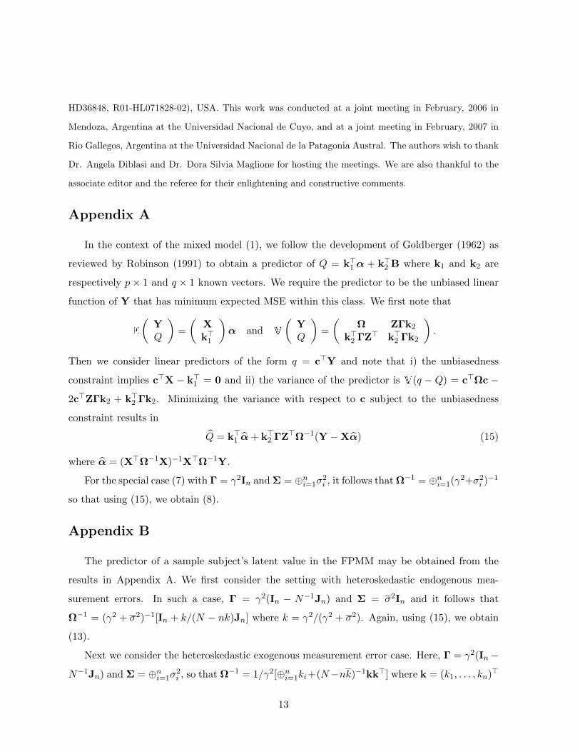
Appendix A

In the context of the mixed model (1), we follow the development of Goldberger (1962) as

reviewed by Robinson (1991) to obtain a predictor of Q = k>1 α + k>2 B where k1 and k2 are

respectively p× 1 and q × 1 known vectors. We require the predictor to be the unbiased linear

function of Y that has minimum expected MSE within this class. We first note that

E

(YQ

)=

(Xk>1

)α and V

(YQ

)=

(Ω ZΓk2

k>2 ΓZ> k>2 Γk2

).

Then we consider linear predictors of the form q = c>Y and note that i) the unbiasedness

constraint implies c>X − k>1 = 0 and ii) the variance of the predictor is V(q − Q) = c>Ωc −

2c>ZΓk2 + k>2 Γk2. Minimizing the variance with respect to c subject to the unbiasedness

constraint results in

Q = k>1 α + k>2 ΓZ>Ω−1(Y −Xα) (15)

where α = (X>Ω−1X)−1X>Ω−1Y.

For the special case (7) with Γ = γ2In and Σ = ⊕ni=1σ

2i , it follows that Ω−1 = ⊕n

i=1(γ2+σ2i )−1

so that using (15), we obtain (8).

Appendix B

The predictor of a sample subject’s latent value in the FPMM may be obtained from the

results in Appendix A. We first consider the setting with heteroskedastic endogenous mea-

surement errors. In such a case, Γ = γ2(In − N−1Jn) and Σ = σ2In and it follows that

Ω−1 = (γ2 + σ2)−1[In + k/(N − nk)Jn] where k = γ2/(γ2 + σ2). Again, using (15), we obtain

(13).

Next we consider the heteroskedastic exogenous measurement error case. Here, Γ = γ2(In−

N−1Jn) and Σ = ⊕ni=1σ

2i , so that Ω−1 = 1/γ2[⊕n

i=1ki+(N−nk)−1kk>] where k = (k1, . . . , kn)>

13

with ki = γ2/(γ2 + σ2i ) and k = n−1∑n

i=1 ki. Then (8) follows directly from (15).

References

Buonaccorsi, J. (2006) Estimation in two-stage models with heteroscedasticity. International

Statistical Review, 74 : 403-418.

Cochran, W.G. (1977). Sampling Techniques. New York: Wiley.

Demidenko, E. (2004). Mixed Models: Theory and Applications. New York: Wiley.

Diggle, P., Heagerty, P., Liang, K-Y. and Zeger, S. (2002). Analysis of Longitudinal Data. New

York: Oxford University Press.

Fitzmaurice, G.M., Davidian, M., Verbeke, M. and Molenberghs, G.(2008). Longitudinal Data

Analysis: A Handbook of Modern Statistical Methods. New York: Chapmann & Hall.

Goldberger, A.S. (1962). Best linear unbiased prediction in the generalized linear regression

model. Journal of the American Statistical Association, 57 : 369-375.

Harville, D.A. (1978). Alternative formulations and procedures for the two-way mixed model.

Biometrics, 34 : 441-453.

Harville, D.A. (1990). In Advances in Statistical Methods for Genetic Improvement of Livestock,

D. Gianola and K. Hammond, eds., 239-276. New York: Springer.

Kennedy, P. (2008). A Guide to Econometrics. Malden, MA: Blackwell Publishing.

Robinson, G.K. (1991). That BLUP Is a good thing: the estimation of random effects. Statis-

tical Science, 6 : 15-51.

San Martino, S., Singer, J.M., and Stanek, E.J. III. (2008). Performance of balanced two-stage

empirical predictors of realized cluster latent values from finite populations: a simulation

study. Journal of Computational Statistics and Data Analysis, 52 : 2199-2217.

Sarndal, C.E., Swensson, B., and Wretman, J. (1992). Model Assisted Survey Sampling. New

York: Springer-Verlag.

Stanek, E.J. III, Well, A. and Ockene, I. (1999). Why not routinely use best linear unbiased

predictors (BLUPs) as estimates of cholesterol, per cent fat from kcal and physical activity?

Statistics in Medicine, 18 : 2943-2959.

14

Stanek, E.J. III and Singer, J.M. (2004). Predicting random effects from finite population

clustered samples with response error. Journal of the American Statistical Association,

99 : 1119-1130.

Stanek, E.J. III, Singer, J.M. and Lencina, V.B. (2004). A unified approach to estimation and

prediction under simple random sampling. Journal of Statistical Planning and Inference,

121 : 325-338.

Stanek, E.J. III and Singer, J.M. (2008). Predicting random effects with an expanded finite

population mixed model. Journal of Statistical Planning and Inference, 138 : 2991-3004.

Sukhatme, P.V. (1984). Sampling Theory of Survey Applications. Ames, IO: Iowa University

Press.

Verbeke, G. and Molenberghs, G. (2001). Linear Mixed Models for Longitudinal Data. New

York: Springer.

Voss, D.T. (1999). Resolving the mixed models controversy. The American Statistician, 53 :

352-356.

15