Prediction: The long and the short of it. - LSEpersonal.lse.ac.uk/MILLNER/files/prediction.pdf · Prediction: The long and the short of it. ... 1An anecdote related by Kenneth Arrow

Prediction: The long and the short of it.

Antony Millner∗1 and Daniel Heyen1

1London School of Economics and Political Science

April 30, 2018

Abstract

Commentators often lament forecasters’ inability to provide precise predictions of the

long-run behaviour of complex economic and physical systems. Yet their concerns of-

ten conflate the presence of substantial long-run uncertainty with the need for long-run

predictability; short-run predictions can partially substitute for long-run predictions if

decision-makers can adjust their activities over time. So what is the relative importance

of short- and long-run predictability? We study this question in a model of rational dy-

namic adjustment to a changing environment. Even if adjustment costs, discount factors,

and long-run uncertainty are large, short-run predictability can be much more important

than long-run predictability.

Keywords: Value of information, prediction, dynamic adjustment, long-run uncertainty

JEL codes: D80, D83

1 Introduction

Ever since Galileo wrote down his laws of motion in the early seventeenth century, the quan-

titative sciences have been engaged in the business of prophesy. Scientific ingenuity has

rendered a staggering range of phenomena more predictable. Atmospheric scientists fore-

cast the weather, epidemiologists predict the spread of infectious diseases, macroeconomists

forecast economic growth, and demographers predict population change. Yet despite many

successes, reliable predictions of the long run behaviour of complex social or natural systems

often remain elusive (Granger & Jeon, 2007; Palmer & Hagedorn, 2006). Inability to predict

the long run is frequently seen as a barrier to effective decision-making, and can be a source of

∗Address: London School of Economics and Political Science, Houghton St, London, WC2A 2AE, UK. Tel:+44 207 107 5423. Email: [email protected]. We are grateful to audiences at EEA, EAERE, Imperial,Heidelberg, LSE, Montpellier, to numerous colleagues (especially Leo Simon, Larry Karp, and Derek Lemoine)for valuable comments, and to the CCCEP and Grantham Foundation for support.

1

emotional distress and planning inertia (Grupe & Nitschke, 2013). Concomitantly, improving

long-run predictability is often a major goal of the scientific communities that produce fore-

casts. But just how important is it to be able to predict the distant future? Does substantial

long-run uncertainty necessarily imply that accurate long-run predictions would be highly

valuable? Or can long-run predictions be effectively substituted by short-run forecasts when

decisions can be adjusted dynamically as new information arrives? This paper attempts to

shed light on these questions.

It is not uncommon to find the presence of long-run uncertainty conflated with the need

for improved long-run predictions.1 For example, a recent report by The National Academy

of Sciences (2016) on planned improvements in long-range weather forecasting suggests that

‘Enhancing the capability to forecast environmental conditions outside the well-developed

weather timescale – for example, extending predictions out to several weeks and months in

advance – could dramatically increase the societal value of environmental predictions, saving

lives, protecting property, increasing economic vitality, protecting the environment, and in-

forming policy choices.’ Similarly, many commentators have suggested that the lack of reliable

projections of the local impacts of climate change, most of which will occur many decades

hence, is a significant barrier to effective adaptation planning. Fussel (2007) contends that

‘the effectiveness of pro-active adaptation to climate change often depends on the accuracy of

[long run] regional climate and impact projections’, while scientists at the World Modelling

Summit for Climate Prediction in 2008 suggested that ‘adaptation strategies require more

accurate and reliable predictions of regional weather and climate...’ (Dessai et al., 2009).

One can find a similar casual identification of the presence of long-run uncertainty with the

importance of long-run predictions in economics. Lindh (2011), for example, states that ‘Very

long-run...forecasts of economic growth are required for many purposes in long-term planning.

For example, estimates of the sustainability of pension systems need to be based on forecasts

reaching several decades into the future.’

While one-shot decisions with fixed lead times between actions and outcomes (e.g. agricul-

tural planting decisions) doubtless benefit from predictability at decision-relevant time-scales,

most long-run decision processes are at least partially flexible, and can thus be adjusted over

time. Firms or individuals who anticipate long-run changes in market conditions, regulation,

or their physical environments will adjust their actions dynamically as new information be-

comes available. Similarly, planners concerned with policies that depend on conditions in

the distant future (e.g. social security) can alter the level of policy instruments (e.g. payroll

taxes) dynamically as the future unfolds. A straightforward identification of the presence

1An anecdote related by Kenneth Arrow (1991) about his time as a military weather forecaster duringWorld War Two provides an extreme example: ‘Some of my colleagues had the responsibility of preparing long-range weather forecasts, i.e., for the following month. The statisticians among us subjected these forecaststo verification and found they differed in no way from chance. The forecasters themselves were convincedand requested that the forecasts be discontinued. The reply read approximately like this: The CommandingGeneral is well aware that the forecasts are no good. However, he needs them for planning purposes.’

2

of long-run uncertainty with the importance of long-run predictions neglects this essential

fact. Since the long-run today will become the short-run tomorrow, short-run predictions can

play an important role in informing decision-making, even when long-run uncertainty is large.

Indeed, it is intuitively clear that short-run predictability is a perfect substitute for long-run

predictability if adjustment is costless. In general however adjustment is costly, and large

abrupt changes in response to short-run warnings are often significantly more costly than

managed gradual transitions which may be informed by long-run predictions. This suggests

that long run predictions could play an important role in informing anticipatory planning,

and avoiding excessive adjustment costs. It is however unclear a priori how the importance

of predictability at different lead times depends on the magnitude of adjustment costs. We

develop a simple analytical model in which this question is answerable.

Our model considers a decision-maker whose period payoffs depend on how well adapted

her choices are to the current state of the world. The state of the world is uncertain, and may

change over time in a non-stationary manner. The decision-maker may adjust her choices in

every period to account for expected changes in her environment, but faces convex adjustment

costs. This cost structure makes rapid adjustments in response to short-run warnings more

costly than gradual incremental shifts of equal magnitude (which may be informed by long-

run predictions).2 Optimal decisions thus balance the benefits of exploiting current conditions

with the need to anticipate future conditions in order to avoid costly rapid adjustments in the

future. The decision-maker has access to a prediction system that generates forecasts of all

future states in every period. These forecasts have a fixed profile of accuracy as a function of

lead time. Thus, if τm is a measure of the accuracy of forecasts of lead time m, the decision-

maker receives a forecast of accuracy τ1, τ2, . . . of states of the world 1, 2, . . . time steps from

the present in every period. For example, the decision-maker receives a forecast of accuracy

τ2 about a state two time steps from now in the current period, but knows that in the next

period she will receive a new forecast of the same state, this time with accuracy τ1. She may

change her decisions in order to react to new predictions once they become available, but

doing so entails a cost. Although the model reduces to a stochastic-dynamic control problem

with an infinite number of state variables, we find a closed-form expression for the decision-

maker’s discounted expected payoffs V as a function of the profile of predictive accuracy that

the prediction system exhibits:

V = V (τ1, τ2, τ3, . . .).

By exploring the dependence of V on its arguments, and the parameters of the decision

problem, we quantify the value of predictability at different lead times. Our central finding is

that if we account for sequential forecast updating and agents’ ability to adjust their activities

2Assuming convex adjustment costs is thus conservative with respect to adjudicating the importance oflong-run predictability, as this assumption favours long-run predictions. See the text following equation (20)below for further discussion.

3

over time, short-run predictability is often more important than long-run predictability, even

if adjustment costs, discount factors, and long-run uncertainty are large.

Although there is a sizeable literature on the value of information and its role in dynamic

decision-making, as far as we know there are few direct antecedents to the questions we

seek to address in this paper. The literature on the value of information began with the

pathbreaking work of Blackwell (1953) and Marschak & Miyasawa (1968), who defined an

incomplete ordering of the ‘informativeness’ of arbitrary information structures. We share

this work’s micro-oriented focus on the value of exogenous information sources for individual

decision-makers, but also differ from it in important respects. In order to ensure tractability,

our model makes strong assumptions about the nature of agents’ payoff functions and the

signals they receive. The return for this specificity is that we are able to study a much richer

set of dynamic decisions than is typically used in this literature. Our focus on the dynamic

characteristics of predictions, i.e. their accuracy as a function of lead time, is absent from

this literature, and necessitates a pared down approach.

Work on the role of information in optimal dynamic decision-making falls into two cat-

egories: two period models that examine the effect of second period learning on optimal

first period decisions (e.g. Arrow & Fisher, 1974; Epstein, 1980), or infinite horizon models

that involve learning about the realizations of a stochastic state variable (e.g. Merton, 1971),

or a parameter of a structural dynamic-stochastic model (e.g. Ljungqvist & Sargent, 2004).

Neither of these standard approaches can capture the effects we study here. Two period

models cannot capture the repeatedly updated nature of prediction and the dependence of

predictability on lead time, both essential features of our model. Finite horizon models also

suffer from an inherent bias towards short-run forecasts, as in a model with horizon H there

will be H lead time 1 forecasts, but only one lead time H forecast. On the other hand, models

based on familiar stochastic processes, or learning about parameters of structural models, do

not usually allow the accuracy of predictions at different lead times to be controlled inde-

pendently, meaning that it is impossible to ask questions about the relative importance of

short- and long-run predictability (see the discussion on p. 8 for an elaboration of this point).

We thus need a different approach if we are to define a model that is tractable, unbiased,

disentangles lead times, and nevertheless retains coarse features of dynamic prediction.

A small applied literature studies the effect of forecasts at different lead times on dynamic

decision-making. Costello et al. (2001) study a finite horizon stochastic renewable resource

model and show that forecasts of shocks more than one step ahead carry no value for a

resource manager. This result follows directly from the fact that their model is linear in the

control variable; this removes the interactions between decisions in different periods, rendering

long-run forecasts irrelevant. Costello et al. (1998) use numerical methods to study the effect

of one and two period ahead forecasts in a calibrated non-linear resource management model,

showing that for some parameter values perfect information at these lead times provides

4

substantial value. Our work considerably generalizes these findings. We analyze a non-

linear model that exhibits non-trivial interactions between time periods, use an infinite time

horizon that removes bias against long-run forecasts, obtain closed-form solutions that enable

clean comparative statics without the need for a calibrated numerical model, calculate the

contribution of forecasts at all lead times to the overall value of a prediction system, and

allow forecasts of arbitrary accuracy.

Finally, a substantial literature delineates the difficulties of long-run forecasting in con-

texts as diverse as climate science, macroeconomics, demography, epidemiology, and national

security (see e.g. Palmer & Hagedorn, 2006; Granger & Jeon, 2007; Lindh, 2011; Lee, 2011;

Myers et al., 2000; Yusuf, 2009). A common refrain in much of this work is that accurate

long-run forecasting is difficult, but would be of considerable value for decision-makers if

achievable. Yet to our knowledge there is no existing analytical framework that provides

intuition for if, and when, this is likely to be true. Our work provides a step towards such a

framework, illustrating in a simple model how a decision-maker’s ability to adapt to changes

in her environment dynamically, and the costs she sustains in doing so, co-determine the

relative importance of short-run and long-run predictability.

2 The model

The model we develop is a variation on a work-horse model of rational dynamic adjustment

to a changing environment that has been deployed in a variety of settings. These include

modeling firm behaviour in the face of changing market conditions (e.g. Sargent, 1978; Fischer

& Blanchard, 1989), and so-called ‘target tracking’ in military and engineering applications.

The model provides a stylized and analytically tractable representation of a class of decision

problems in which a decision-maker’s period payoffs depend on an exogenously changing

environmental variable, and changes in activities incur adjustment costs. We discuss our

model’s assumptions and how they differ from existing work below, but first spell out the

details.

Consider a decision-maker who faces an uncertain exogenous environment at each time

n ∈ N. The units of time are arbitrary, but should be understood to match the frequency of

forecast updates (e.g. days for weather forecasts, quarters for inflation forecasts). We assume

that the decision-maker’s possible choices can be mapped into the real line, and denote a

generic choice by X ∈ R. We will operate at a high level of abstraction, and thus leave the

interpretation of X open. The more literal-minded reader is referred to Appendix A, where we

provide a direct interpretation of the decision problem we examine in terms of a competitive

firm making production decisions in the face of uncertain future prices. Other interpretations

are of course possible, e.g. X could be the level of a tax set by a regulator, or an individual’s

stock of defensive capital.

5

The decision-maker may adjust X in each period, at a cost that is convex in the magni-

tude of the adjustment. Since large abrupt changes in activities are more costly than gradual

incremental shifts of equal magnitude, the decision-maker has an incentive to engage in antic-

ipatory planning. The state of the world at time n, denoted by θn ∈ R, is the loss-minimizing

decision in that period. Values of X that are closer to θn are better adapted to conditions at

time n, and give rise to higher period payoffs. The decision-maker’s choices must achieve a

balance between exploiting current conditions (i.e. choosing X close to the current expected

value of θ) and preparing for future conditions (i.e. shifting X towards expected future values

of θ), thus avoiding excessively large and costly adjustments later on.

For any time n, let θt = θn+t for t ≥ 0, i.e. θt is the value of the loss-minimizing decision

θ that will be realized t time steps in the future (see Figure 1 below for an illustration). We

denote the agent’s beliefs about θt at time n by pn(θt). At n = 0 the agents’ prior beliefs

about the future values θt are captured by an infinite sequence of normal distributions with

means µ0t and precisions (i.e. inverse variance) λ0

t , i.e.

p0(θt) ∼ N (µ0t , 1/λ

0t ). (1)

The values of µ0t and λ0

t are unconstrained, allowing us to describe a wide variety of beliefs

about the future. In particular, we do not require the agent to believe that the environmental

random variable θ is identically distributed over time.

Let Xn be the value of the decision variable X that the agent inherits at the beginning of

period n. At the beginning of the period the agent chooses a new value for X, i.e. Xn+1. This

is the value of X that will affect payoffs in the current period, and be passed forward to the

next period. The cost of modifying the decision variable from Xn to Xn+1 is 12α(Xn+1−Xn)2,

where α ≥ 0 is a parameter that captures the magnitude of the adjustment costs the agent

faces. After the choice of Xn+1 is made, the agent experiences the realization of the current

value of θ, i.e. θ0, and sustains a loss equal to half the squared distance between Xn+1 and

θ0. Thus, the expected period payoff at the beginning of the current period is given by,

W (Xn+1, Xn, pn(θ0)) = −1

2

[∫(Xn+1 − θ0)2pn(θ0)dθ0 + α(Xn+1 −Xn)2

]. (2)

The decision-maker’s objective function is the usual discounted sum of expected period pay-

offs, which will be defined in full below. As advertised, the reader seeking an interpretation

of this payoff function in a familiar economic application is referred to Appendix A.

To model the effect of predictions on the agent’s beliefs, we assume that at the end of

each period n, the agent receives a sequence of forecasts Sn = (snt )t≥1 of the values of future

states θt for all t ≥ 1. We assume that

snt = θt + εnt (3)

6

where

εnt ∼ N (0, 1/τt) (4)

and τt ≥ 0 is the precision of forecasts of events t time steps ahead. Thus predictions have

an exogenous profile of precision as a function of lead time, parameterized by the infinite

sequence of parameters

~τ ≡ (τ1, τ2, τ3, . . .).

The precision sequence ~τ is time invariant, i.e. the prediction system is assumed to produce

forecasts with the same profile of accuracy as a function of lead time at every time n.3

Consider two prediction systems A and B, with precision sequences ~τA, ~τB. If, for a fixed

lead time t, τAt > τBt , then A is more informative (in the sense of Blackwell (1953)) than

B about events t time steps in the future. Although in practice we would expect ~τ to be a

decreasing sequence, we place no constraints on its value in what follows.

Notice that the agent receives a new sequence of forecasts Sn at the end of every period

n. However, the precision of the information she receives about a particular value θk that lies

in her future changes as time progresses and she moves closer to time k. Since the agent’s

prior beliefs about the future values θt in period n = 0 are normal, and the conditional

distributions of signals st given states are normal, her beliefs about the future values of

the states will update according to the standard normal-normal Bayesian formulae (see e.g.

DeGroot, 1970). In particular, beliefs about future values θt will be normally distributed in

every period, and are characterized by a mean µnt and precision λnt in period n. Moreover,

the agent also knows that the beliefs she currently holds about the future values θt for t ≥ 1,

will become her beliefs about θt−1 in the next period. For example, her current beliefs about

the next period will become her beliefs about the current period, in the next period. Using

these observations, we can write down the state equations that describe how the forecasting

system changes the agents’ beliefs about the values of the states θt from one period to the

next:

µn+1t (snt+1) =

τt+1

τt+1 + λnt+1

snt+1 +λnt+1

τt+1 + λnt+1

µnt+1

λn+1t = λnt+1 + τt+1. (5)

As is standard in the normal-normal bayesian updating model, the posterior mean of beliefs

about each future value θt is a convex combination of the prior mean and the signal realization,

with the weight that is placed on the signal increasing in the signal precision. Posterior

precisions, however, evolve deterministically. A complete description of the current state of

3While we make this assumption for simplicity and clarity, we note that any covariance stationary timeseries satisfies the time invariance property. We mention this not because our model is covariance stationary(it need not be), but to illustrate that this property is not unusual.

7

the system at the beginning of period n is thus given by the ordered pair (Xn, Yn), where

Yn ≡ ((µnt )t≥0, (λnt )t≥0), (6)

collects together the infinitely many ‘belief’ state variables. The dynamics of Yn are given

by (5), and Xn is a ‘decision’ state variable whose next value is chosen by the agent in each

period. Figure 1 provides a graphical summary of the model setup, and the timing of events.

Before proceeding to the solution of the model, we now discuss some of its more unusual

assumptions, why they are necessary, and how they relate to existing work. The payoff

structure in the model, captured by (2), is formally identical to that in previous models

of dynamic adjustment we alluded to at the beginning of this section. The novelty in our

approach arises from our representation of the decision-maker’s dynamic expectations, i.e.

the updating process summarized in (5). In existing applications of the dynamic adjustment

model the loss-minimizing decisions θ are always modeled as a stochastic process. Sargent

(1978), for example, assumes that θn follows an AR(1) process. However, this approach

cannot be used if we are to gain traction on our central question, i.e. understanding the

relative importance of short- and long-run predictability. To understand why, suppose that

the θn are correlated (as they would be if modeled as a stochastic process), and that a

prediction system provides information about some θk. Then learning about θk means that

we learn something about all values of θn. It is thus not possible to associate a prediction

about an event at a given lead time with a change in uncertainty at only that lead time

in a correlated model. Our central question is thus generically unanswerable in correlated

models, unless the correlation structure can be fine-tuned to generate arbitrary patterns of

predicability as a function of lead time.4 Hence our assumption that the θn are independent

(but not identically distributed).5 By contrast, the belief updating system described in (5)

retains several features of dynamic prediction (i.e. sequentially updated expectations, and

predictions whose accuracy depends on lead time), but allows us to control the precision of

predictions at each lead time independently. The cost of this approach is that instead of being

able to describe dynamic expectations with a single state variable as in standard stochastic

process models, we now require an infinite number of state variables, one for each independent

belief about each future event. In sum, while the independence assumption may seem unusual

to some readers, it is a necessary expediency if we are to generate insights into the relative

4This could be possible in models where the state equation depends on many lagged variables (e.g. AR(n)models), however one needs an infinite number of lags to disentangle all lead times, the relationship betweenparameters of the state equation and predictability at different lead times is highly complex, and such mod-els severely constrain agents’ prior beliefs about the future due to their stationarity. In addition, dynamicoptimization problems in these high lag environments are often intractable. By contrast our stylized modelparsimoniously captures lead time dependent predictive accuracy, maintains tractability, and allows us todescribe prior uncertainty in a flexible manner. Costello et al. (1998) use a similar independence assumption.

5Of course, if the θn are independent a priori, but the signals snt are correlated, this induces correlationbetween time periods after a single forecast is received. We thus also require the snt to be independent.

8

n=1

n=0

1 2 3 4

t

t

0

1 2 3 0

Figure 1: Illustration of the model setup. The figure depicts the agent’s beliefs, choices, andthe information provided by the prediction system, in the first two periods n = 0, 1. At thebeginning of period n = 0 the agent holds a sequence of prior beliefs about the future valuesof the state of the world θt. Beliefs about each future value of θt are normally distributed,indicated by the dark blue distributions at each value of t. The initial value of the decisionvariable is X = X0, and the agent must choose a new value X1 at the beginning of the period.At the end of the period the agent receives the infinite sequence of forecasts S0 = (s0

t )t≥1,indicated by the dark red dots, which allow her to update her beliefs about the future valuesθt. The brown distributions at each t capture the agent’s initial expectations about the signalss0t she will receive (i.e. q(s0

t ;Y0) in (7)). Smaller values of τt, which are assumed to occurat longer lead times in this example, correspond to wider distributions of expected forecastrealizations, and weaker belief updating towards the realized signal. This is demonstrated bythe agent’s updated beliefs at n = 1, where once again beliefs about future values of θt atthe beginning of the period appear in dark blue, and for comparison the agent’s n = 0 beliefsand signal realizations are represented by the light blue distributions and dots respectively.Once again, the agent must choose a new value for the decision variable X2 at the beginningof the period n = 1, and will receive a new sequence of forecasts S1 = (s1

t )t≥1 (indicated bydark red dots), with the same profile of precisions at the end of period n = 1.

9

importance of predictability at different lead times.6 We now turn to the model’s solution.

Bellman equation

Let V (Xn, Yn) be the current value of the infinite dimensional state (Xn, Yn), where Yn is

defined in (6). The next period value of the state depends on the sequence of signals Sn that

the agent will receive at the end of the current period. At the beginning of period n the

agent’s beliefs about signal snt (t ≥ 1) are given by:

q(snt ;Yn) =

∫p(snt |θt)pn(θt)dθt

∼ N (µnt , 1/λnt + 1/τt), (7)

where the last line follows from a simple calculation using (3–4). We denote the agent’s beliefs

about the probability of receiving a sequence of signals Sn = (snt )t≥1 by

Q(Sn;Yn) =∞∏t=1

q(snt ;Yn). (8)

We are now ready to state the Bellman equation for the value function V (Xn, Yn). Denote

the next period value of the belief states Yn+1 as a function of the previous value Yn and the

realized signal sequence Sn as

Yn+1 = F (Yn, Sn). (9)

where F (Yn, Sn) is given by (5). Then,

V (Xn, Yn) = maxXn+1

W (Xn+1, Xn, Yn) + β

∫V (Xn+1, F (Yn, S

n))Q(Sn;Yn)dSn, (10)

where dSn =∏∞t=1 ds

nt , β ∈ (0, 1) is the agent’s discount factor, and we have changed no-

tation slightly to emphasize the dependence of the period payoff function (2) on the belief

state variables Yn. Note that the dependence of the value function on the profile of forecast

precisions ~τ comes both through the updating rule F (Yn, Sn) (see eq. (5)), and through the

agent’s expectations about the values of future forecast realizations (see eq. (7)). Thus, in-

creases in predictability affect both the quality of future decisions (by reducing the variance

of outcomes), and the agent’s expectations about the information that will be available in the

future.

Optimal policy

The model is a stochastic dynamic control problem with an infinite number of state variables,

since the agent holds an independent belief about each future value θt. Despite the infinite

6Sequential event forecasts of the kind we consider have been studied in e.g. Clements (1997); Selten (1998).

10

dimensionality of the state space in our model,7 standard methods based on the Benveniste-

Scheinkman condition (Benveniste & Scheinkman, 1979) yield simple closed form solutions

for the optimal control rule. We state this rule in some detail, as it will help us to interpret

the main results below. All proofs can be found in the appendices.

Proposition 1. The optimal policy Xn+1 = π(Xn, Yn) is given by

π(X,Y ) = aX +∞∑t=0

btµt (11)

where

a =1 + α(1 + β)−

√(1 + α(1 + β))2 − 4α2β

2αβ,

bt =a

α(aβ)t .

It is straightforward to demonstrate the following properties of the coefficients a, bt:

a+∞∑t=0

bt = 1

limα→0

a = 0, limα→∞

a = 1,∂a

∂α> 0

limα→0

bt =

{1 t = 0

0 t > 0, limα→∞

bt = 0

∂

∂α

(bt+1

bt

)> 0,

∂b0∂α

< 0.

Proposition 1 thus shows that the optimal policy function π(X,Y ) chooses the next value of

X to be a convex combination of the current value of X and the expected values of θt. The

policy rule exhibits the certainty equivalence property, i.e. it is independent of the agent’s

uncertainty about future events. This is a well-known consequence of the quadratic payoff

function in our model, which makes the model tractable (e.g. Ljungqvist & Sargent, 2004).

Although the policy rule does not depend on uncertainty, the value function certainly will,

and it is it’s dependence on the precision profile ~τ that we are ultimately interested in.

The coefficients of the policy rule have an intuitive dependence on the adjustment cost

7The curse of dimensionality normally renders stochastic-dynamic control problems in state spaces of evenmoderate dimension (e.g. more than 10) intractable. Our model is, as far as we know, the only example of anon-trivial stochastic-dynamic model on an infinite dimensional state space that admits an exact closed-formsolution for the value function.

11

parameter α. Consider the extreme cases α→ 0, and α→∞. The proposition shows that

limα→0

π(X,Y ) = µ0

limα→∞

π(X,Y ) = X.

When adjustment costs tend to zero, the policy rule does not depend on either X or µt

for t ≥ 1. This occurs since with costless adjustment the decision problem separates into a

sequence of static optimization problems, and the payoff maximizing choice in each of these

problems is simply to choose X equal to the expected value of the current value of θ, i.e.

µ0. When α → ∞, any change in the value of X is very costly, so the optimal action is to

leave X where it is. In between these extremes the policy rule depends on expectations about

all future values of θt. As α increases from zero the decision maker’s choice depends more

on both the inherited value of X, and her expectations about the future. This occurs since

the convexity of adjustment costs penalizes large adjustments later on. Current choices thus

account for both the benefits of adjusting to current conditions and the need to anticipate

future conditions. The larger is α, the more important it is to anticipate future conditions,

and this is reflected in the fact that coefficients bt decrease at a slower rate as α increases. At

the same time, larger α makes adjustments more costly, leading the policy rule to place greater

weight on the inherited value of X. Finally, to understand the finding that a+∑∞

t=0 bt = 1,

consider the case in which µt = X for all t. In this case the agent believes that her choice

is perfectly adapted to conditions now and in the future, and she should thus not want to

change X. This occurs if aX +∑∞

t=0 btX = X.

It will be helpful in what follows to have some quantitative understanding of which values

of α are ‘large’ and ‘small’ in some absolute sense. To benchmark how α affects optimal

policies, consider a deterministic version of the model in which the states θn are chosen to be

a fixed sequence of draws from an arbitrary univariate random variable with finite variance.

When α = 0, optimal decisions coincide with the current value of θn, i.e. Xn = µ0 = θn for

all n. As α increases, adjustment becomes more costly, and the values of Xn fluctuate less

than θn itself. Appendix C derives an expression for the asymptotic variance of the policy

choices Xn as a function of α and β. For a wide range of β, α > 1.5 implies that the decision

maker adjusts to less than 20% of the variability in θ, and α > 3 implies adjustment to less

than 10% of the variability. Thus, α = 3 is already a fairly large value of the adjustment cost

parameter. In addition, the appendix demonstrates that changes in α have a greater effect

on behaviour when α is small (e.g. α < 1) than when it is large.

Value function

In order to understand the effect of the precision sequence ~τ on the agent’s expected payoffs,

we need to compute the value function. This would seem to be difficult, as the model’s state

12

space is infinite dimensional, the period payoff depends non-quadratically8 on the precision

state variables λt, and we need to take expectations of the value function over an infinite

sequence of signals, the distribution of which depends on all the belief state variables. Despite

these apparent obstacles it is possible to obtain a closed form solution for the value function,

which enables the remainder of our analysis.

Begin by defining a shift operator ∆ that acts on infinite vectors ~Z = (zt)t≥0 as follows:

∆(~Z) = ∆((z0, z1, z2, . . .)) ≡ (z1, z2, z3, . . .).

Thus ∆ simply deletes the first element of ~Z and shifts all the other elements forward one

position. The belief updating rule (5) for the vector of prior precisions ~λ = (λt)t≥0 can thus

be written as:

F (~λ) = ∆(~λ) + ~τ , (12)

where F (~λ) denotes the ~λ components of the updating rule in (5). Define F tk(~λ) to be the

(k+ 1)-th element of F t(~λ).9 In addition, recall that bk is the coefficient of µk in the optimal

control rule (11). Then,

Proposition 2. The value function V (X,Y ) is given by

V (X,Y ) = T (~τ) + terms independent of ~τ ,

where

T (~τ) ≡ −1

2b0

[ ∞∑t=1

βt∞∑k=0

(bkb0

)2 1

F tk(~λ)

](13)

∝ −[(

1

λ1 + τ1+ (a2β2)

1

λ2 + τ2+ (a2β2)2 1

λ3 + τ3+ . . .

)+ β

(1

(λ2 + τ2) + τ1+ (a2β2)

1

(λ3 + τ3) + τ2+ (a2β2)2 1

(λ4 + τ4) + τ3+ . . .

)+ β2

(1

(λ3 + τ3 + τ2) + τ1+ (a2β2)

1

(λ4 + τ4 + τ3) + τ2+ (a2β2)2 1

(λ5 + τ5 + τ4) + τ3+ . . .

)+O(β3)

].

8From (2) we have

W (Xn+1, Xn, Yn) = −1

2

[(1 + α)X2

n+1 + αX2n − 2Xn+1(µ0 + αXn) +

1

λn0+ (µn0 )2

].

One could write this payoff in terms of the variance of the agent’s beliefs about θt, making it linear in variances,but then the state equations for the evolution of variances would be non-linear (see (5)). Standard methodsfrom linear quadratic control are not applicable.

9For example,

F 2(~λ) = F (F (~λ)) = F (∆(~λ) + τ) = ∆(∆(~λ) + ~τ) + ~τ = ∆2(~λ) + ∆(~τ) + ~τ.

Thus say F 20 (~λ) = λ2 + τ2 + τ1, where it is important to recall that ~τ = (τ1, τ2, . . .).

13

To interpret this result notice that the term∑∞

k=0

(bkb0

)21

F tk(~λ)in (13) represents the

contribution to the value function from the uncertainty the agent faces when she takes a

decision t time steps in the future. 1/F tk(~λ) is the agent’s uncertainty about events that are

k time steps in the future, in period t. The exponentially declining factor (bk/b0)2 = (a2β2)k

captures the importance of uncertainty about events at temporal distance k for decision-

making, as can be seen from the optimal policy rule (11). T (~τ) is thus the discounted

sum of the cost of uncertainty for each future decision. The forecasting system reduces this

uncertainty cost by providing information about all future periods, in every period. The

agent’s uncertainty about events that are k time steps in the future in a period t time steps

from now is reduced by forecasts of precision τt+k, τt+k−1, . . . , τk.

3 The relative value of short- and long-run predictability

The previous section derived an expression for the decision-maker’s value function for an

arbitrary prediction system that obeys (5). In this section we unpack this result in order to

study the relative importance of short- and long-run predictability. Given prior uncertainty~λ = (λt)t≥1, the function T (~τ) in Proposition 2 depends on the sequence of forecast precisions

~τ . Our goal now is to understand the dependence of T (~τ) on its arguments. In general this

is a complex task, as T (~τ) is a non-separable function of the τm. The following subsections

consider different methods for extracting the information T (~τ) contains about the relative

importance of predictability at different lead times.

3.1 Marginal predictability

To make initial progress we begin by finding a linear approximation to T (~τ) at ~τ = ~0.

This approximation will only be accurate when forecast precisions are marginal. Studying

a linearized version of T (~τ) has two purposes. First, the linear approximation to T (~τ) is

a separable function of ~τ , allowing the contribution of each τm to the value function to

be computed easily in this case. This allows us to form clear intuition for the effects that

determine the relative importance of different lead times, to first order. Second, and more

importantly, in this approximation all interactions between forecast lead times are neglected.

Since we expect the interesting effects in the model to be a consequence of the sequential

updating of forecasts, which allow short-run predictability to partially substitute for long-

run predictability, it is useful to first examine a baseline case in which those substitution

effects (i.e. interactions between lead times) are effectively switched off. This will allow us to

demonstrate later on how accounting for interactions between lead times alters the relative

importance of short- and long-run predictability.

14

Begin by defining the function

g(m) ≡∞∑k=0

βk

λ2m+k

, (14)

and assuming that

limt→∞

λ2t+1

λ2t

> β, (15)

implying that g(m) is finite for all m (by the ratio test). Then,

Proposition 3. If the interactions between forecast lead times are neglected, the increase in

the value function due to the prediction system (relative to an uninformative baseline) is

dV = T (d~τ)− T (~0) ≈ a

α(1− a2β)

∞∑m=1

rmdτm, (16)

where

rm ≡ g(m)βm(1− (a2β)m

). (17)

To understand the intuition behind this result we now derive it heuristically (the appendix

contains a formal proof). Recall that the agent receives a forecast of lead time m in every pe-

riod. The effect of the forecast the agent receives in the current period is to reduce uncertainty

about events at temporal distance m. But, in doing so, this forecast gives rise to a cascade of

uncertainty reductions at shorter lead times in future periods. This occurs since a reduction

in uncertainty about lead time m events in the current period is equivalent to a reduction

in uncertainty about events at lead time m − 1 in the next period, and lead time m − 2 in

the period after that, etc. As (13) makes clear, the value of a reduction in uncertainty about

events k time steps in the future is proportional to (bk/b0)2 = (a2β2)k. Since uncertainty

reductions in future periods are discounted, a marginal unit of precision in the first forecast

of lead time m that the agent receives increases payoffs by an amount proportional to

m−1∑k=0

βm−k(a2β2)k = βmm−1∑k=0

(a2β)k.

Because a marginal increase in the precision of forecasts of lead time m increases payoffs in

proportion to ddλm

(−1/λm) = 1/λ2m, the total effect of the first forecast of lead time m is to

increase payoffs by an amount proportional to

1

λ2m

βmm−1∑k=0

(a2β)k.

This quantity accounts for the uncertainty reduction effect of the first forecast of lead time m,

which the agent receives at the end of the current period. At the end of the next period, the

15

agent receives another forecast of lead time m. This forecast gives rise to the same cascade of

uncertainty reductions, and has the same value as the initial forecast, up to a normalization.

The normalization is simply the discounted value of the change in lead time m uncertainty

that the agent faces in the next period, i.e. β 1λ2m+1

. This occurs in all future periods. Thus,

the total value of a marginal unit of precision in forecasts of lead time m is proportional to:

1

λ2m

(βm

m−1∑k=0

(a2β)k

)+

β

λ2m+1

(βm

m−1∑k=0

(a2β)k

)+

β2

λ2m+2

(βm

m−1∑k=0

(a2β)k

)+ . . .

∝

( ∞∑t=0

βt

λ2m+t

)βm(1− (a2β)m

)This is exactly the expression we obtained in (17). Notice how the derivation of this expression

makes it clear that sequential updating of forecasts is not a major determinant of the value

of a marginal unit of predictability. The fact that forecasts are updated sequentially gives

rise to the factor(∑∞

t=0βt

λ2m+t

)= g(m) in (17), but if only a single marginal forecast of lead

time m were received in the first period, the expression in (17) would look very similar, with

this factor simply replaced by 1λ2m

. Thus, neglecting the interactions between lead times is

qualitatively similar to neglecting sequential forecast updating itself (we make this analogy

exact in a special case below).

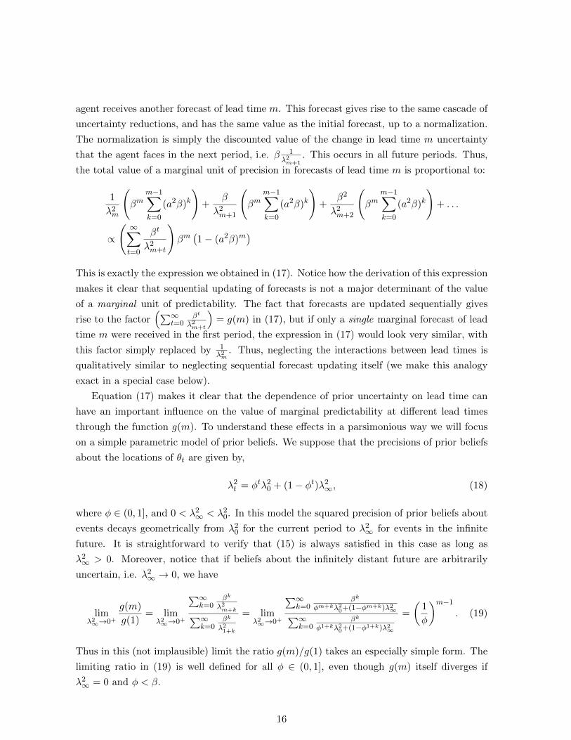
Equation (17) makes it clear that the dependence of prior uncertainty on lead time can

have an important influence on the value of marginal predictability at different lead times

through the function g(m). To understand these effects in a parsimonious way we will focus

on a simple parametric model of prior beliefs. We suppose that the precisions of prior beliefs

about the locations of θt are given by,

λ2t = φtλ2

0 + (1− φt)λ2∞, (18)

where φ ∈ (0, 1], and 0 < λ2∞ < λ2

0. In this model the squared precision of prior beliefs about

events decays geometrically from λ20 for the current period to λ2

∞ for events in the infinite

future. It is straightforward to verify that (15) is always satisfied in this case as long as

λ2∞ > 0. Moreover, notice that if beliefs about the infinitely distant future are arbitrarily

uncertain, i.e. λ2∞ → 0, we have

limλ2∞→0+

g(m)

g(1)= lim

λ2∞→0+

∑∞k=0

βk

λ2m+k∑∞k=0

βk

λ21+k

= limλ2∞→0+

∑∞k=0

βk

φm+kλ20+(1−φm+k)λ2∞∑∞k=0

βk

φ1+kλ20+(1−φ1+k)λ2∞

=

(1

φ

)m−1

. (19)

Thus in this (not implausible) limit the ratio g(m)/g(1) takes an especially simple form. The

limiting ratio in (19) is well defined for all φ ∈ (0, 1], even though g(m) itself diverges if

λ2∞ = 0 and φ < β.

16

In the limit as λ2∞ → 0, we can thus define a simple measure of the value of a unit of

predictability about events at distance m, relative to the value of a unit of predictability

about events at distance 1:

Rm ≡rmr1

= βm−1︸ ︷︷ ︸Discounting

(1

φ

)m−1

︸ ︷︷ ︸Uncertainty

[1− (a2β)m

1− a2β

]︸ ︷︷ ︸Early warning

. (20)

Using this expression, the relative value of the predictability of events at different lead times

may be computed as a function of the three parameters α, β and φ. These parameters char-

acterize the decision-maker’s flexibility, impatience, and prior uncertainty about the future

respectively. Aside from being simple to analyze, the choice of priors in (18) makes the for-

mulas for rm/r1 for updating from a single forecast vs. updating from sequential forecasts

coincide exactly in the limit as λ2∞ → 0, since 1/λ2m

1/λ21= g(m)/g(1) in this case. To a first

approximation there is thus no difference between once-off and sequential forecasting in this

model of priors. This is thus an especially good baseline from which to assess how account-

ing for the interactions between lead times alters the balance between short- and long-run

predictability.

The formula (20) shows that there are three effects that determine the relative value of

marginal predictability at different lead times. First, since forecasts at larger lead times relate

to more distant payoffs, they are more heavily discounted. This gives rise to the first term

in (20), which is decreasing in m. Second, since the prior precision of beliefs is smaller for

larger lead times (i.e. uncertainty increases with the time horizon), and payoffs are concave

in precisions, the effect of a marginal increase in the precision of beliefs is increasing in lead

times. This leads to the second term in (20), which is increasing in m, reflecting the fact

that the long-run is more uncertain than the short-run. Finally, the third term captures the

cumulative effect of an early warning about events at lead time m on all subsequent decisions

that are made until that event is realized. Since warnings of lead time m give rise to improved

decision-making for m− 1 subsequent adjustment decisions, longer lead times are associated

with greater cost savings. Thus the third term in (20) is increasing in m, reflecting the fact

that earlier warnings give rise to cheaper adjustments (since adjustment costs are convex). It

is moreover straightforward to verify that

∂2

∂α∂m

[1− (a2β)m

1− a2β

]> 0

when m ≥ 1. Thus, the larger are adjustment costs α, the faster the third term in (20)

increases with m. This is intuitive, since the more costly adjustments are, the more important

it is to get early warning of the need for them (again due to convexity). This term thus

17

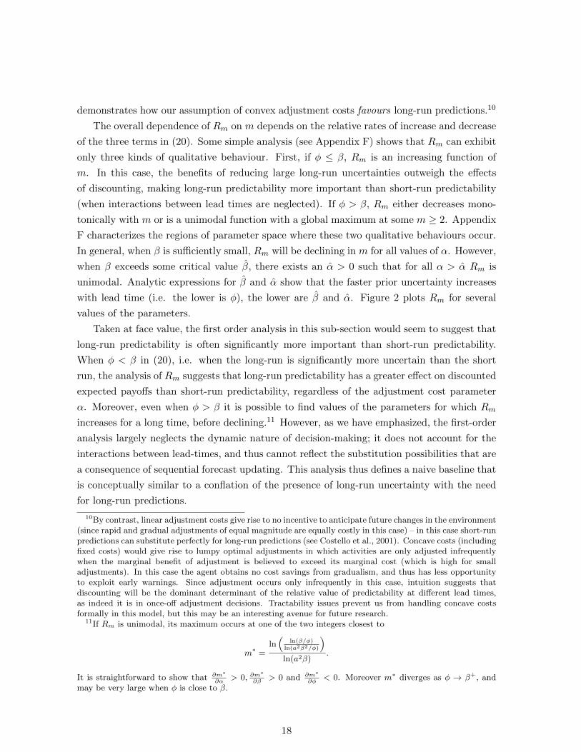
demonstrates how our assumption of convex adjustment costs favours long-run predictions.10

The overall dependence of Rm on m depends on the relative rates of increase and decrease

of the three terms in (20). Some simple analysis (see Appendix F) shows that Rm can exhibit

only three kinds of qualitative behaviour. First, if φ ≤ β, Rm is an increasing function of

m. In this case, the benefits of reducing large long-run uncertainties outweigh the effects

of discounting, making long-run predictability more important than short-run predictability

(when interactions between lead times are neglected). If φ > β, Rm either decreases mono-

tonically with m or is a unimodal function with a global maximum at some m ≥ 2. Appendix

F characterizes the regions of parameter space where these two qualitative behaviours occur.

In general, when β is sufficiently small, Rm will be declining in m for all values of α. However,

when β exceeds some critical value β, there exists an α > 0 such that for all α > α Rm is

unimodal. Analytic expressions for β and α show that the faster prior uncertainty increases

with lead time (i.e. the lower is φ), the lower are β and α. Figure 2 plots Rm for several

values of the parameters.

Taken at face value, the first order analysis in this sub-section would seem to suggest that

long-run predictability is often significantly more important than short-run predictability.

When φ < β in (20), i.e. when the long-run is significantly more uncertain than the short

run, the analysis of Rm suggests that long-run predictability has a greater effect on discounted

expected payoffs than short-run predictability, regardless of the adjustment cost parameter

α. Moreover, even when φ > β it is possible to find values of the parameters for which Rm

increases for a long time, before declining.11 However, as we have emphasized, the first-order

analysis largely neglects the dynamic nature of decision-making; it does not account for the

interactions between lead-times, and thus cannot reflect the substitution possibilities that are

a consequence of sequential forecast updating. This analysis thus defines a naive baseline that

is conceptually similar to a conflation of the presence of long-run uncertainty with the need

for long-run predictions.

10By contrast, linear adjustment costs give rise to no incentive to anticipate future changes in the environment(since rapid and gradual adjustments of equal magnitude are equally costly in this case) – in this case short-runpredictions can substitute perfectly for long-run predictions (see Costello et al., 2001). Concave costs (includingfixed costs) would give rise to lumpy optimal adjustments in which activities are only adjusted infrequentlywhen the marginal benefit of adjustment is believed to exceed its marginal cost (which is high for smalladjustments). In this case the agent obtains no cost savings from gradualism, and thus has less opportunityto exploit early warnings. Since adjustment occurs only infrequently in this case, intuition suggests thatdiscounting will be the dominant determinant of the relative value of predictability at different lead times,as indeed it is in once-off adjustment decisions. Tractability issues prevent us from handling concave costsformally in this model, but this may be an interesting avenue for future research.

11If Rm is unimodal, its maximum occurs at one of the two integers closest to

m∗ =ln(

ln(β/φ)

ln(a2β2/φ)

)ln(a2β)

.

It is straightforward to show that ∂m∗

∂α> 0, ∂m

∗

∂β> 0 and ∂m∗

∂φ< 0. Moreover m∗ diverges as φ → β+, and

may be very large when φ is close to β.

18

2 4 6 8 10 12 14 16 18 20

Lead time (m)

0

0.5

1

1.5

2

2.5

3

3.5

4

4.5R

m

α = 0.25, φ = 1

α = 4, φ = 1

α = 4, φ = 0.9

Figure 2: Typical dependence of Rm on adjustment costs (α) and prior uncertainty (φ).β = 0.95 in these examples.

3.2 Accounting for interactions

In this section we move beyond first-order results, aiming to summarize the dependence of

T (~τ) on ~τ in a manner that accounts for the interactions between lead times. It is intuitively

clear that these interactions are important determinants of the overall value of a prediction

system. If we are able to predict events at lead time m very accurately, the value of an

improvement in the predictability of events at lead time m + 1 must surely be quite low.

Indeed, inspection of the expression for T (~τ) in (13) shows that for any positive integers m, k,

∂T

∂τm> 0,

∂2T

∂τm∂τk< 0.

Thus, T (~τ) is a concave function of ~τ ; predictabilities at different lead times are substitutes.

Since T (~τ) is a non-separable function of the infinite vector of parameters ~τ = (τm)m≥1, there

is no unique way of computing the contribution of each individual τm to the value function.

We will exploit the fact that T (~τ) is concave in ~τ to present a measure of the importance of

19

different lead times that we find especially intuitive.

In order to summarize the dependence of T (~τ) on its arguments we imagine that the

decision-maker has a hypothetical total predictability budget B =∑∞

m=1 τm, and study how

she would like this budget to be allocated between lead times. Since T (~τ) is concave this

allocation problem has a unique solution, and the budget share allocated to each lead time

captures its importance in a manner that accounts for interactions. We emphasize that the

predictability budget B is a purely hypothetical construct; it does not represent the costs of

increasing predictability, which are very likely to vary by lead time. Rather, B is merely a

mathematical device that allows us to summarize the relative importance of predictability at

different lead times in the value function. As in the rest of the value of information literature,

our focus throughout the paper is on the benefit side of predicability.

Formally, we are interested in computing the following quantity:

~σ ≡ 1

B

(argmax~τ T (~τ) s.t.

∞∑m=1

τm = B

). (21)

The m-th component of ~σ, denoted σm, is the share of the total predictability budget B that

the agent would like to allocate to lead time m. By definition, σm ∈ [0, 1] for all m, and∑∞m=1 σm = 1. Although it is not possible to solve for ~σ analytically, it is straightforward to

find an arbitrarily good approximation to the solution using standard numerical constrained

optimization routines.

In general ~σ depends on the vector of prior precisions ~λ. To maintain consistency with the

marginal analysis of the previous section, we assume that λt = φt/2λ0, corresponding to the

λ2∞ → 0 limit of (18). The relative importance of prior beliefs and predictions in determining

the expectations that enter the value function is captured by the ratio λ0/B. To see this,

notice from (13) that the optimization problem in (21) is equivalent to finding a sequence of

values ~σ that maximizes

− 1

B

[(1

λ0B φ

1/2 + σ1

+ (a2β2)1

λ0B φ

2/2 + σ2

+ (a2β2)2 1λ0B φ

3/2 + σ3

+ . . .

)

+ β

(1

(λ0B φ2/2 + σ2) + σ1

+ (a2β2)1

(λ0B φ3/2 + σ3) + σ2

+ (a2β2)2 1

(λ0B φ4/2 + σ4) + σ3

+ . . .

)+O(β2)

],

subject to∑

m σm = 1. When λ0/B � 1, predictions are highly non-marginal relative to

the prior, and dominate the value function. Interactions between forecast lead times will be

most important in this case. By contrast, when λ0/B � 1 predictions are marginal relative

to the prior, and interactions between lead times are of second order importance. So what

is a reasonable value of λ0/B? It is clear that if we want to study substitution between

lead times we must not choose λ0/B to be too large. On the other hand, if λ0/B is very

small the prior plays no role in the analysis. This case is of interest (see below), but we

20

would also like to investigate the role of the prior, so we cannot only choose small values

for λ0/B. In practice, we would expect forecast errors to be roughly comparable to prior

uncertainty. Indeed, for many phenomena forecasts themselves are responsible for forming

our priors. Our current uncertainty about climate change, for example, is intimately related

to the uncertainty in scientific projections of climate change. We will thus initially work with a

conservative representative value of λ0/B = 1. Note that this implies that the sum of forecast

precisions over all lead times is comparable in size to the precision of our beliefs about the

current period. Almost all σm are thus small relative to λ0/B. Indeed, the importance of

the prior is likely overestimated in this parameterization. Appendix G contains a sensitivity

analysis and detailed discussion of the cases where λ0/B � 1 and λ0/B � 1. Figure 3

demonstrates the typical dependence of ~σ on adjustment costs α and prior uncertainty φ

when λ0/B = 1.

Several features of Figure 3 deserve highlighting. First, the budget allocations in this

figure tell a very different story from the marginal analysis in Figure 2. Even when φ < β (i.e.

the top panel in Fig. 3) so that the long run is significantly more uncertain than the short

run, the decision-maker would like to allocate most of her predictability budget to short lead

times, i.e. 1-4 time steps ahead. By contrast, the analysis in Fig. 2 showed that the value

of a marginal unit of predictability is increasing in lead time when φ < β; at face value this

would seem to suggest that the decision-maker should allocate her entire budget to long-run

prediction. The results in Fig. 3 are very different, because ~σ accounts for the substitution

possibilities between lead times that arise from sequential forecast updating. These substitu-

tion effects favour the short-run because accurate short-run forecasts can compensate for any

errors in long-run forecasts once the long-run events in question come nearer to the present, in

addition to providing information about current near-term conditions. If adjustment is highly

costly (i.e. α is large) it is clearly more costly to react to short-run warnings, and accurate

early warnings become more important. This is reflected in the fact that ~σ places larger

weight on long lead times as α increases. However, perhaps surprisingly, even for very large

values of α substitution effects cause the agent to allocate very small budget shares to lead

times larger than 10 times steps. The presence of predictability at these shorter lead times

renders long-run predictability essentially irrelevant. Fig. 3 also shows that prior uncertainty

does not have nearly as large an effect on how the decision-maker would like to allocate her

predictability budget as the marginal analysis suggested it might. The two panels of Fig. 3,

which correspond to values of φ below and above β respectively, differ in their details, with

lower values of φ (i.e. greater long-run uncertainty) giving rise to greater weight on longer

lead times. But in both cases very little weight is given to long lead times. In contrast, the

marginal analysis suggested that these cases should give rise to very different behaviour, with

long-run forecasts always being more valuable than short-run forecasts when φ < β. This

indicates that substitution effects dominate the role of the prior in determining the budget

21

2 4 6 8 10 12 14

Lead time (m)

0

0.1

0.2

0.3

0.4

0.5

0.6

0.7

σm

φ = 0.9 < β

α = 2-2

α = 2-1

α = 1

α = 2

α = 22

α = 23

2 4 6 8 10 12 14

Lead time (m)

0

0.1

0.2

0.3

0.4

0.5

0.6

0.7

0.8

σm

φ = 1 > β

α = 2-2

α = 2-1

α = 1

α = 2

α = 22

α = 23

Figure 3: Budget share σm allocated to lead time m in the optimization problem in (21).β = 0.95, λ0B = 1.

allocation, despite the precision of the prior being comparable to or greater than that of

predictions.

While Fig. 3 pertains to the baseline case λ0/B = 1, it is also interesting to examine

~σ when λ0/B → 0. In this limit the agent’s beliefs about all future periods are entirely

determined by the prediction system, the prior plays no role. In this case ~σ captures the

22

2 4 6 8 10 12 14

Lead time (m)

0

0.1

0.2

0.3

0.4

0.5

0.6

σm

α = 2-2

α = 2-1

α = 1

α = 2

α = 22

α = 23

Figure 4: Budget share σm allocated to lead time m in the optimization problem in (21).β = 0.95, λ0B → 0. This figure illustrates the ‘pure’ effect of substitution between lead times,when priors play no role in the analysis.

‘pure’ effects of substitution between lead times, unadulterated by the prior (which favours

long lead times). Results for this case are depicted in Fig. 4. This figure clearly demonstrates

how substitution between lead times leads the decision-maker to place most of his budget on

short run predictability, even when adjustment costs are very large.

4 Conclusions

We have developed a simple analytical model that allows us to compute decision-makers’

induced preferences over prediction systems with different profiles of accuracy as a function

of lead time. Valuing prediction systems correctly requires an explicitly dynamic model that

accounts for the fact that forecasts of events at different temporal distance have different

accuracies, and that agents may adapt their decisions to new information as forecasts are

updated over time. The essential novel feature of our model is that it disentangles the pre-

dictability of events at different temporal distances, allowing us to compute the contribution

of predictive accuracy at each lead time to the overall value of a forecasting product in a

23

simple and tractable manner. This enables a study of the relative importance of short- and

long-run predictability that is, we believe, novel in the literature.

Our results point to potentially important lessons for decision-makers, and for efforts to

improve the social value of forecasts. As observed in the introduction, it is not uncommon

to find the presence of long-run uncertainty conflated with a need for long-run predictability

in policy circles. In general however this is a logical fallacy, as it neglects decision-makers’

abilities to adjust activities over time in response to updated forecasts. Our analysis suggests

that if adjustments in response to sequential forecast updates are accounted for, short-run

predictability is often more valuable than long-run predictability, even if adjustment costs

and long-run uncertainty are large. It is perhaps surprising just how effectively short-run

predictability can substitute for long-run predictability in our model, as the convexity of

adjustment costs would seem to imply that accurate long-run forecasts would give rise to

significant cost savings when adjustment costs are large. The fact that this result would be

difficult to guess a priori (at least for us) points to the necessity of modeling approaches

that aim to disentangle the contribution of predictions at each lead time to the overall value

of forecasts. Such models could also provide forecast producers with valuable information

about where they should focus their efforts at forecast improvement. While improvements

in long-run predictions often require new scientific approaches that reduce model misspecifi-

cation errors, short-run predictions can often be substantially improved by simply reducing

measurement errors in initial conditions (i.e. increasing the quality of observations). Our

results suggest that the latter activity may carry significant value for decision-makers con-

cerned with adapting to long-run changes, even though such improvements will yield little

new information about long-run conditions.

Although we believe that our model provides important conceptual insights into the de-

terminants of rational demand for predictability at different lead times, it is clearly limited in

some respects. The modeling exercise is made possible by judicious assumptions which render

an otherwise impossibly complex infinite dimensional stochastic control problem solvable in

closed form. We highlight two of these assumptions here.

First, the model relies on a location-independent quadratic loss function. It is clear that if

some states of the world are intrinsically more valuable than others, information about these

states will be of greater importance. Since our model assumes a payoff function that penalizes

actions purely according to their distance from a state-dependent optimal choice, the costs of

a maladapted choice do not depend on the state of the world. It is therefore best to think of

our results as defining a symmetric baseline case in which the ability of the decision-maker to

adapt to her environment is not state-contingent. We believe that this captures the essence of

the problems we are interested in, but extensions to asymmetric loss functions would naturally

be of interest, although we expect them to face analytical difficulties.

Second, as in the rest of the value of information literature, our model focuses on a

24

decision-maker who faces an exogenously changing environment. Thus, its conceptual lessons

apply to e.g. individuals and firms, but less to large entities whose actions may strongly affect

the uncertainties in their operating environments. For example, we feel that the model is a

fair abstract representation of the problem of adapting to climate change at the local level,

but not of mitigating climate change at the global level. In the latter case actions the world

takes to reduce greenhouse gas emissions clearly affect uncertainties, whereas in the former

any small country or firm may reasonably take changes in the climate as exogenous to its own

activities.

References

K. J. Arrow (1991). ‘”I Know a Hawk From a Handsaw”’. In M. Szenberg (ed.), Eminent

Economists: Their Life Philosophies. Cambridge University Press, Cambridge England ;

New York.

K. J. Arrow & A. C. Fisher (1974). ‘Environmental Preservation, Uncertainty, and Irre-

versibility’. The Quarterly Journal of Economics 88(2):312–319.

L. M. Benveniste & J. A. Scheinkman (1979). ‘On the Differentiability of the Value Function

in Dynamic Models of Economics’. Econometrica 47(3):727–732.

D. Blackwell (1953). ‘Equivalent Comparisons of Experiments’. The Annals of Mathematical

Statistics 24(2):265–272.

M. P. Clements (1997). ‘Evaluating the Rationality of Fixed-event Forecasts’. Journal of

Forecasting 16(4):225–239.

C. Costello, et al. (1998). ‘The Value of El Nino Forecasts in the Management of Salmon: A

Stochastic Dynamic Assessment’. American Journal of Agricultural Economics 80(4):765–

777.

C. Costello, et al. (2001). ‘Renewable resource management with environmental prediction’.

Canadian Journal of Economics 34(1):196–211.

M. DeGroot (1970). Optimal Statistical Decisions. McGraw-Hille, New York, WCL edition

edn.

S. Dessai, et al. (2009). ‘Climate prediction: A limit to adaptation?’. In W.N. Adger, I. Loren-

zoni, & K. O’Brien (eds.), Adapting to Climate Change: Thresholds, Values, Governance,

pp. 64–78. Cambridge University Press.

L. G. Epstein (1980). ‘Decision Making and the Temporal Resolution of Uncertainty’. Inter-

national Economic Review 21(2):269–283.

25

S. Fischer & O. Blanchard (1989). Lectures on Macroeconomics. MIT Press.

H.-M. Fussel (2007). ‘Vulnerability: A generally applicable conceptual framework for climate

change research’. Global Environmental Change 17(2):155–167.

C. W. J. Granger & Y. Jeon (2007). ‘Long-term forecasting and evaluation’. International

Journal of Forecasting 23(4):539–551.

D. W. Grupe & J. B. Nitschke (2013). ‘Uncertainty and anticipation in anxiety: an integrated

neurobiological and psychological perspective’. Nature Reviews Neuroscience 14(7):488–

501.

R. Lee (2011). ‘The outlook for Population Growth’. Science 333:569–573.

T. Lindh (2011). ‘Long-horizon growth forecasting and demography’. In M. P. Clements &

D. F. Hendry (eds.), Oxford handbook of economic forecasting. Oxford University Press.

L. Ljungqvist & T. J. Sargent (2004). Recursive Macroeconomic Theory. MIT Press, Cam-

bridge, Mass, 2nd edn.

J. Marschak & K. Miyasawa (1968). ‘Economic Comparability of Information Systems’.

International Economic Review 9(2):137–174.

R. C. Merton (1971). ‘Optimum consumption and portfolio rules in a continuous-time model’.

Journal of Economic Theory 3(4):373–413.

M. F. Myers, et al. (2000). ‘Forecasting disease risk for increased epidemic preparedness in

public health’. Advances in Parasitology 47:309–330.

National Academy of Sciences (2016). Next genertaion earth system prediction: Strategies

for subseasonal to seasonal foreacasts. doi:https://doi.org/10.17226/21873. The National

Academies Press, Washington D.C.

T. Palmer & R. Hagedorn (eds.) (2006). Predictability of Weather and Climate. Cambridge

University Press.

T. J. Sargent (1978). ‘Estimation of Dynamic Labor Demand Schedules under Rational

Expectations’. Journal of Political Economy 86(6):1009–1044.

R. Selten (1998). ‘Axiomatic Characterization of the Quadratic Scoring Rule’. Experimental

Economics 1(1):43–61.

M. Yusuf (2009). ‘Prediction Proliferation: The History of the Future of Nuclear Weapons’.

Tech. rep., Brookings Institution Policy Paper no. 11.

26

Appendix

A A microeconomic interpretation of the model

Here we provide an interpretation of our model in a familiar microeconomic setting. Consider

a competitive firm that produces a quantity qt of product at time t, and faces linear marginal

costs of production C ′(q) = c0 + c1q. The firm faces uncertain prices (pt)t≥0 in the future,

and quadratic adjustment costs k(qt − qt−1)2. These costs are a reduced form representation

of costs sustained due to rejigging operations at the intensive and extensive margins. Small

changes in production are handled at the intensive margin, and are thus cheap – current

employees work longer/shorter hours, installed capital is used more/less intensively, and orders

from existing suppliers are tweaked to meet small fluctuations in demand. However, large

changes in production require extensive margin changes – large numbers of new employees

must be hired/fired, new machinery must be bought or rented, and new suppliers found and

terms negotiated. The form of our adjustment costs amounts to assuming that extensive

margin adjustments are cheaper if done in a planned sequence of steps, rather than in an

abrupt transition. There are several reasons why this might be. With early warning the

firm could find creative ways of adapting its existing resources to new market conditions.

Early warning may also place the firm in a stronger negotiating position with respect to

employment and supply contracts (because of the lack of urgency), and could reduce the

opportunity costs associated with under/over capacity. Quadratic adjustment costs are an

analytically convenient reduced form way of representing these inertial forces on adjustment.

Since the firm takes prices pt as given, its instantaneous profit function can be written as:

Πt = ptqt − (c0qt +1

2c1q

2t )− k(qt − qt−1)2

= −c1

2(qt − θt)2 − k(qt − qt−1)2 +Mt

where θt = (pt − c0)/c1, and Mt is a decision irrelevant constant, which may be neglected

when computing the value of information about the sequence of values (θt)t≥0. Thus the

firm’s profit function is of the form (2), up to an irrelevant factor of c1.

B Proof of Proposition 1

We use the Bellman equation (10) to solve for the optimal policy function Xn+1 = π(Xn, Yn).

When referring to functions and operations on functions, we will adopt a notation in which

primed variables denote next period quantities, and unprimed variables denote current period

quantities, i.e. W = W (X ′, X, Y ) and V = V (X,Y ). So ∂W∂X′ , for example, refers to the

function whose value is the partial derivative of W with respect to its first argument, i.e. the

next period value of X. When we evaluate functions and their derivatives at specific times,

27

we will still use e.g. Xn, Xn+1 to denote function arguments. Thus ∂W∂X′ (Xn+1, Xn, Yn) is the

partial derivative of W with respect to its first argument, evaluated at (Xn+1, Xn, Yn). With

this notation, the first order condition for Xn+1 is

∂W

∂X ′(π(Xn, Yn), Xn, Yn) + β

∫∂V

∂X(π(Xn, Yn), F (Yn, S))Q(S;Yn)dS = 0. (22)

By the envelope theorem,

∂V

∂X(Xn, Yn) =

∂W

∂X(π(Xn, Yn), Xn, Yn) (23)

From (2), and (23) evaluated at time n+ 1, we have

∂W

∂X ′(π(Xn, Yn), Xn, Yn) = µ0 + αXn − (1 + α)π(Xn, Yn)

∂V

∂X(π(Xn, Yn), F (Yn, S)) =

∂W

∂X(π(π(Xn, Yn), F (Yn, S)), π(Xn, Yn), F (Yn, S))

= α(X ′ −X)∣∣X′=π(π(Xn,Yn),F (Yn,S)),X=π(Xn,Yn)

= α(π(π(Xn, Yn), F (Yn, S))− π(Xn, Yn)).

Substituting into (22), we find that the policy rule must satisfy

µ0 + αXn − (1 + α)π(Xn, Yn) + β

∫[α(π(π(Xn, Yn), F (Yn, S))− π(Xn, Yn))]Q(S;Yn)dS = 0.

(24)

We solve this equation by the ‘guess and verify’ method. The certainty equivalence property

of the quadratic control problem suggests that we should look for a control rule of the form

π(X,Y ) = aX +

∞∑t=0

btµt

where the coefficients (a, (bt)t≥0) are to be determined. Plugging this guess into (24), and

now suppressing the index n, we find:

[µ0 + αX − (1 + α)(aX +

∞∑t=0

btµt)]+

βα

[∫ (a(aX +

∞∑t=0

btµt) +

∞∑t=0

btµ′t(st+1)− (aX +

∞∑t=0

btµt)

)Q(S, Y )dS

]= 0

28

where µ′t(st+1) is the next period value of µt conditional on receiving a signal st+1, given by

(5). Since Estµ′t(st+1) = µt+1, we can simplify this to:

µ0 + αX − (1 + α)(aX +∞∑t=0

btµt)+

β[αa2X + aα

∞∑t=0

btµt + α

∞∑t=0

btµt+1 − aαX − α∑t

btµt] = 0.

Since this equation must hold for all values of X,µt, we must equate the coefficients of each

state variable to zero. The equation for the coefficient of X is:

αβa2 − (1 + α(1 + β))a+ α = 0 (25)

⇒a =1 + α(1 + β)±

√(1 + α(1 + β))2 − 4α2β

2αβ(26)

To pick the correct root, note that if α→ 0, the policy rule should reduce to

π(X,Y ) = µ0.

This follows since when adjustment is costless, the optimal policy simply maximizes period

payoffs. For the positive root we have

limα→0

a(α)→∞,

thus giving incorrect behaviour. By contrast, we show below that the correct behaviour is

obtained if we select the negative root. Thus we conclude that

a = a(α, β) =1 + α(1 + β)−

√(1 + α(1 + β))2 − 4α2β

2αβ(27)

The equation for b0 is:

1− (1 + α)b0 + aβαb0 − αβb0 = 0

⇒b0 =1

1 + α+ αβ(1− a). (28)

For t ≥ 1, the equation for bt is:

− (1 + α)bt + aβαbt + αβbt−1 − αβbt = 0

⇒bt =αβ

1 + α+ αβ(1− a)bt−1.

29

Thus for all t ≥ 0,

bt =1

1 + α+ αβ(1− a)

[αβ

1 + α+ αβ(1− a)

]t(29)

We can simplify this further by using the equation for a in (25). Define

Λ ≡ 1 + α+ αβ(1− a) (30)

From (25) we have

(αβ)a2 − (1 + α(1 + β))a+ α = 0

Now

1 + α(1 + β) = Λ + αβa

⇒ (αβ)a2 − (Λ + αβa)a+ α = 0

⇒ Λ =α

a.

Thus

bt =a

α(aβ)t . (31)

We now prove the properties of the coefficients a, bt, stated below the proposition:

1. limα→0 a(α, β) = 0

Use l’Hopital’s rule: differentiate the numerator and denominator of a with respect to

α, and evaluate the limit of each as α→ 0:

limα→0

a(α, β) =1 + β − 1

2×1(2× 1× (1 + β)− 0)

2β

= 0.

2. limα→∞ a(α, β) = 1:

limα→∞

a(α, β) =1 + β

2β− 1− β

2β

= 1.

3. ∂a∂α > 0.

From (27) we have

∂a

∂α= −1

2

−αβ +√α2(1− β)2 + 2α(1 + β) + 1− α− 1

α2β√α2(1− β)2 + 2α(1 + β) + 1

. (32)

30

Hence, ∂a∂αa > 0 iff

− αβ +√α2(1− β)2 + 2α(1 + β) + 1− α− 1 < 0

⇐⇒√α2(1− β)2 + 2α(1 + β) + 1 < 1 + α+ αβ

⇐⇒ α2(1− β)2 + 2α(1 + β) + 1 < α2(1 + β)2 + 2α(1 + β) + 1

which is obviously satisfied for all α > 0, β ∈ (0, 1).

4. a+∑∞

t=0 bt = 1.

From the previous calculations we know that a ∈ [0, 1] ⇒ aβ ∈ [0, 1]. It follows from

(31) that

a+

∞∑t=0

bt − 1 = a+a

α

1

1− aβ− 1

=−αβa2 + a(1 + α(1 + β))− α

α(1− aβ)

= 0

where the last equality follows from the defining equation for a in (25).

5. ∂∂α(bt+1/bt) > 0, ∂b0

∂α < 0.

Since a+∑∞

t=0 bt = 1, and a is increasing in α, we know that∑∞

t=0 bt must be decreasing

in α. From (31) we see thatbt+1

bt= aβ

and hence this ratio is increasing in α. Since bt declines more slowly as α increases, it

must be the case that ∂b0∂α < 0 in order to ensure that

∑∞t=0 bt is decreasing in α.

C Illustration of the dependence of optimal policies on adjust-

ment costs α.

To illustrate how the adjustment cost parameter α affects decisions quantitatively, consider

a deterministic version of the model in which the values θn are chosen be a fixed sequence

of draws from an arbitrary univariate random variable with finite variance σ2. When α = 0,

optimal decisions coincide with the current value of θn, i.e. Xn = µ0 = θn for all n. As α

increases, adjustment becomes more costly, and the values of Xn fluctuate less than θn itself.

31

0 5 10 15 20

α

0

0.1

0.2

0.3

0.4

0.5

0.6

0.7

0.8

0.9

1

limn→∞

Va

r(X

n,X

n+

1,

)/σ

2β = 0.5

β = 0.75

β = 0.9

β = 0.99

Figure 5: Asymptotic variability of the decision variable X relative to the variability of theloss-minimizing decisions θ, assuming that the values of θn are deterministic and given by afixed sequence of draws from a random variable with variance σ2.

Using the formula (11) and some simple ergodic arguments one can show that

limn→∞

Var(Xn, Xn+1, . . .) =

∑∞t=0 b

2t

1− a2σ2

=

[( aα

)2 1

(1− a2)(1− a2β2)

]σ2

for arbitrary initial condition X0. Figure 5 plots the asymptotic variance of the sequence of

decisions as a function of α for several β. The figure illustrates how α controls the magnitude

of the adjustments the decision-maker makes to adapt to fluctuations in a stationary envi-

ronment. For a wide range of β, α > 1.5 implies that the decision maker adjusts to less than

20% of the variability in θ, and α > 3 implies adjustment to less than 10% of the variability.

In addition, changes in α have a greater effect on behaviour when α is small (e.g. α < 1)

than when it is large.

32

D Proof of Proposition 2

As in the derivation of the optimal policy function, we use the ‘guess and verify’ method.

Begin by guessing that the value function has the form

V (X,Y ) = kX2 +∞∑t=0

ctµtX +∞∑t=0

∞∑p=t+1

Dt,pµtµp +∞∑t=0

dtµ2t +

∞∑t=0

∞∑i=0

fi,tλt + hi,t

. (33)

All except the last term of this expression are straightforward to guess simply by inspection of

the formula for the period payoff in (2). The last term will however be the most important, as

it will turn out that this is the only term that depends on the precision sequence ~τ = (τt)t≥1.

Consider the quadratic terms in this guess of the form µtµp. We are going to need to know

how these will transform under the updating rule (5) and after the expectation over signal

realizations has been applied. Letting a prime denote the next period value of a variable, we

are interested in computing expectations of the form

ESµ′tµ′p = Est+1,sp+1µ

′t(st+1)µ′p(sp+1)

where signals are distributed according to the agents’ current posterior predictive distribution,

given by (7). Recall that

µ′t(st+1) =τt+1

τt+1 + λt+1st+1 +

λt+1

τt+1 + λt+1µt+1

When t 6= p, we can immediately write down the answer, as means are martingales, and

signals are independent:

Est+1,sp+1µ′t(st+1)µ′p(sp+1) = µt+1µp+1

For t = p however, things are different:

Est+1µ′t(st+1)µ′t(st+1) = Est+1

[τt+1

τt+1 + λt+1st+1 +

λt+1

τt+1 + λt+1µt+1

]2

Consider the quadratic term in st+1 in this expression:

Est+1

(τt+1

τt+1 + λt+1

)2

s2t+1 =

(τt+1

τt+1 + λt+1

)2

[Var(st+1) + µ2t+1]

=

(τt+1

τt+1 + λt+1

)2

[λt+1 + τt+1

λt+1τt+1+ µ2

t+1]

=τt+1

λt+1(λt+1 + τt+1)+

(τt+1

τt+1 + λt+1

)2

µ2t+1

33

When we combine this expression with the other terms in the expression for Est+1µ′t(st+1)µ′t(st+1),

the factor in front of µ2t+1 in the second term will cancel to 1 (as occurs in the case t 6= p),

and we are left with

Est+1µ′t(st+1)µ′t(st+1) =

τt+1

λt+1(λt+1 + τt+1)+ µ2

t+1. (34)

Hence, in summary:

Est+1,sp+1µ′t(st+1)µ′p(sp+1) =

{µt+1µp+1 t 6= pτt+1

λt+1(λt+1+τt+1) + µ2t+1 t = p.

(35)

It will be more convenient in what follows to write the terms that depend on λt+1 is this

expression asτt+1

λt+1(λt+1 + τt+1)=

1

λt+1− 1

λt+1 + τt+1. (36)

We now want to write down the Bellman equation for our assumed functional form for the

value function. The first step is to compute the period payoff:

W (π(X,Y ), X, Y ) = −1

2

[(1 + α)[π(X,Y )]2 + αX2 − 2π(X,Y )(µ0 + αX) +

1

λ0+ (µ0)2

]= −1

2

[(1 + α)(aX +

∞∑t=0

btµt)2 + αX2 − 2(aX +

∞∑t=0

btµt)(µ0 + αX) +1

λ0+ (µ0)2

]

= −1

2

(1 + α)(a2X2 + 2aX

∞∑t=0

btµt +

∞∑t=0

∞∑p=t+1

2btbpµtµp +

∞∑t=0

b2tµ2t ) + αX2

−2aXµ0 − 2aαX2 − 2µ0

∞∑t=0

btµt − 2αX∞∑t=0

btµt + (µ0)2 +1

λ0

]

We also have

ESV (π(X,Y ), F (Y, S)) = ES

k(π(X,Y ))2 +∞∑t=0

ctµ′t(st+1)π(X,Y ) +

∞∑t=0

∞∑p=t+1

Dt,pµ′t(st+1)µ′p(sp+1)

+∞∑t=0

dt(µ′t(st+1))2 +

∞∑i=0

∞∑t=0

fi,tλ′t + hi,t

]

= k[aX +∑t

btµt]2 +

∞∑t=0

ctµt+1[aX +

∞∑p=0

bpµp] +

∞∑t=0

∞∑p=t+1

Dt,pµt+1µp+1

+

∞∑t=0

dt(µt+1)2 +

∞∑t=0

dt

[1

λt+1− 1

λt+1 + τt+1

]+

∞∑i=0

∞∑t=0

fi,tλt+1 + τt+1 + hi,t

We now have expressions for each of the three terms V (X,Y ),W (π(X,Y ), X, Y ),ESV (π(X,Y ), F (Y, S)),

34

and must choose the free coefficients of the value function so that

V (X,Y ) = W (π(X,Y ), X, Y ) + βESV (π(X,Y ), F (Y, S))

holds as an identity. We begin by focussing on the terms that depend on λt. If we focus just

on these terms, the Bellman equation reads

∞∑i=0

∞∑t=0

fi,tλt + hi,t

= −1

2

1

λ0+ β

( ∞∑t=0

dt

[1

λt+1− 1

λt+1 + τt+1

]+∞∑i=0

∞∑t=0

fi,tλt+1 + τt+1 + hi,t

)(37)

We must determine values for the sequences fi,t, hi,t such that this equation holds as an

identity. Since the right hand side of this equation contains terms of the form 1/λt for all t,

we must have terms of this form on the left hand side as well. We thus begin by choosing

h0,t = 0

for all t ≥ 0. Then if (37) is to hold as an identity for all λt, τt we require

f0,0 = −1

2(38)

f0,t = βdt−1 for t ≥ 1. (39)

Notice that setting h0,t = 0 creates an imbalance of terms of the form

∞∑t=0

f0,t

λt+1 + τt+1

on the right hand side of the Bellman equation through the last term in (37). To correct this

imbalance through terms on the left hand side, we must choose

h1,t = τt

implying in turn that we must choose

f1,0 = 0

f1,t = β[−dt−1 + f0,t−1] for t ≥ 1.

Again we create an imbalance of terms on the right hand side, which we correct by picking

h2,t = τt + h1,t−1 = τt + τt−1

35

and we find that

f2,0 = 0

f2,t = βf1,t−1.

We can complete this imbalance/rebalance procedure indefinitely to solve for all the coeffi-

cients fi,t, hi,t. We find:

h0,t = 0; hi,t = τt + hi−1,t−1 i ≥ 1 (40)

f0,0 = −1

2; f0,t = βdt−1 t ≥ 1 (41)

f1,0 = 0; f1,t = β[−dt−1 + f0,t−1] t ≥ 1 (42)

fi,0 = 0; fi,t = βfi−1,t−1. n ≥ 2, t ≥ 1. (43)

It is straightforward to solve the set of recurrence relations for fi,t. It is convenient to write

the solution as an infinite dimensional matrix:

f =

−12 βd0 βd1 βd2 βd3 . . .

0 −β(d0 + 12) β(βd0 − d1) β(βd1 − d2) β(βd2 − d3) . . .

0 0 −β2(d0 + 12) β2(βd0 − d1) β2(βd1 − d2) . . .

0 0 0 −β3(d0 + 12) β3(βd0 − d1) . . .

......

......

... . . .

(44)

The i, t entry of this matrix corresponds to fi−1,t−1, i.e. the rows correspond to fixed values

of i, and the columns to fixed values of t, both starting at zero.12

Clearly fi,t = 0 for any i > t. Thus the only parameters hi,t that are relevant have

12Notice that∑∞i=0 fi,t = − 1

2βt. To understand this suppose that τt = 0 for all t, i.e. the agent receives

no forecasts. Then her beliefs will not change over time, and the variance of her beliefs about θn+t will bethe same once time n + t rolls around as they are in the current period n. The contribution of the varianceterms to the value function in this case is thus straightforward to compute, since variance terms only enter theperiod payoff through the term − 1

2λ0. Thus, when τt = 0, we should expect the following term in the value

function: − 12

∑∞t=0 β

t 1λt

. Now when τt = 0 for all t, we have

∞∑i=0

∞∑t=0

fi,tλt + hi,t

=

∞∑t=0

∑∞i=0 fi,t

λt

= −1

2

∞∑t=0

βt1

λt

as expected.

36

0 ≤ i ≤ t. It is straightforward to solve the recurrence relation (40) to find

h0,t = 0

hi,t =t∑

k=t+1−iτk, 1 ≤ i ≤ t

The matrix f makes it clear that we will need to understand the parameters dt if we are to

solve for fi,t. We can find these parameters by solving the µ2t terms of the Bellman equation.

Define

δi,j =

{1 i = j

0 i 6= j(45)

Then the Bellman equation for the µ2t terms yields

dt = −1

2[(α+ 1)(bt)

2 + (1− 2b0)δt,0] + β(k(bt)2 + ct−1bt(1− δt,0) + dt−1(1− δt,0)

=

(kβ − 1

2(α+ 1)

)(bt)

2 − 1

2(1− 2b0)δt,0 + βct−1bt + βdt−1 (46)

where d−1 ≡ 0 ≡ c−1. This equation in turn depends on the coefficients of X2 and µtX, i.e.

k and ct. The X2 terms of the Bellman equation give:

k = −1

2((1 + α)a2 + α− 2aα) + β(ka2)

⇒ k = −1

2

((1 + α)a2 + α− 2aα

1− βa2

), (47)

which is a known quantity. As a check, another way to compute k is to use the envelope

theorem result:

∂V

∂X= α(π(X,Y )−X)

= α((a− 1)X +∑t

btµt)

Integrating this, we should find that

k = αa− 1

2.

Using (25) it can be shown that these two formulae for k agree, and we thus use the second,

simpler, expression.

37

Equating coefficients of the µtX terms in the Bellman equation gives:

ct = −1

2((1 + α)2abt − 2aδt,0 − 2αbt) + β(2kabt + act−1(1− δt,0))

= (α− a(1 + α) + 2βka)bt + aδt,0 + aβct−1

Consider the factor in front of bt in this expression. Substituting k = α2 (a−1) into this factor

we see that it is equal to

αβa2 − a(1 + α(1 + β)) + α

But from the definition of a in (25) this expression is identically zero. Thus ct satisfies

ct = aδt,0 + aβct−1

where c−1 = 0. Thus, we conclude that

ct = a(aβ)t (48)

for all t ≥ 0.

Equation (46) thus becomes:

dt =

(αβ

a− 1

2− 1

2(α+ 1)

)b2t +

(b0 −

1

2

)δt,0 + (aβ)tbt + βdt−1

= −1

2(1 + α+ αβ(1− a))b2t + (aβ)tbt + (b0 −

1

2)δt,0 + βdt−1

From (29) and the definition of Λ in (30) we have

bt =1

Λ

(αβ

Λ

)t.

Thus

d0 = −Λ

2b20 + b0 −

1

2

= −Λ

2(

1

Λ)2 +

1

Λ− 1

2

=1

2(

1

Λ− 1)

Also for t ≥ 1:

dt = − 1

2Λ

(αβ

Λ

)2t

+ (aβ)t1

Λ

(αβ

Λ

)t+ βdt−1

= − 1

2Λ

(αβ

Λ

)2(αβΛ

)2(t−1)

+1

Λ

aαβ2

Λ

(aαβ2

Λ

)t−1

+ βdt−1

38

This is a non-homogeneous first order difference equation. The solution for t ≥ 1 is

dt = βtd0 −1

2Λ

(αβ

Λ

)2 t−1∑k=0

βt−k−1

(αβ

Λ

)2k

+1

Λ

aαβ2

Λ

t−1∑k=0

βt−k−1

(aαβ2

Λ

)k

= βtd0 −1

2Λ

(αβ

Λ

)2

βt−1t−1∑k=0

(α2β

Λ2

)k+

1

Λ

aαβ2

Λβt−1

t−1∑k=0

(aαβ

Λ

)k

= βtd0 −1

2Λ

(αβ

Λ

)2

βt−1

(1− (α2β/Λ2)t

1− α2β/Λ2

)+

1

Λ

aαβ

Λβt

1−(aαβΛ

)t1− aαβ

Λ

= βt

1

2Λ− 1

2− 1

2Λ

α2β

Λ2

(1− (α2β/Λ2)t

1− α2β/Λ2

)+

1

Λ

aαβ

Λ

1−(aαβΛ

)t1− aαβ

Λ

Since Λ = α

a we see that

α2β

Λ2=aαβ

Λ= a2β.

Thus the solution for dt simplifies to

dt =1

2βt[a

α− 1 +

a

α

a2β

1− a2β(1− (a2β)t)

]. (49)

We can use this solution for dt, and the matrix f to find an explicit solution for the

coefficients fi,t. Let i = t− n where 1 ≤ n < t. Then the matrix f shows that

ft−n,t = βt−n(βdn−1 − dn)

= βt−n[β

(1

2βn−1

[a

α− 1 +

a

α

a2β

1− a2β(1− (a2β)n−1)

])− 1

2βn[a

α− 1 +

a

α

a2β

1− a2β(1− (a2β)n)

]]= −1

2βt−n

a

α(aβ)2n

For t = i ≥ 1, f gives

ft,t = −βt(d0 +1

2)

= −βt[

1

2(a

α− 1) +

1

2

]= −1

2βta

α.

Thus we conclude that for any t ≥ 1, 1 ≤ i ≤ t,

fi,t = −1

2

a

αβi(aβ)2(t−i).

The values of f0,t and fi,0 can be read directly off the matrix f . Summarizing these results,

39

the terms of interest to us are given by:

T (~τ) =

∞∑t=1

t∑i=1

fi,tλt + hi,t

(50)

where for t ≥ 1, 1 ≤ i ≤ t,

hi,t =t∑

k=t+1−iτk, (51)

fi,t = −1

2

a

αβt(a2β)t−i. (52)

Using the definition of F tk(~λ) as the (k+ 1)-th element of F t(~λ), where F (~λ) is given by (12),

we can reorder the terms of the sum in our expression for T (~τ) to see that

T (~τ) =− 1

2

aβ

α

[(1

λ1 + τ1+ (a2β2)

1

λ2 + τ2+ (a2β2)2 1

λ3 + τ3+ . . .

)+ β

(1

(λ2 + τ2) + τ1+ (a2β2)

1

(λ3 + τ3) + τ2+ (a2β2)2 1

(λ4 + τ4) + τ3+ . . .

)+β2

(1

(λ3 + τ3 + τ2) + τ1+ (a2β2)

1

(λ4 + τ4 + τ3) + τ2+ (a2β2)2 1

(λ5 + τ5 + τ4) + τ3+ . . .

)+ . . .

]=− 1

2

aβ

α

[(1

F0(~λ)+ (a2β2)

1

F1(~λ)+ (a2β2)2 1

F2(~λ)+ . . .

)

+ β

(1

F 20 (~λ)

+ (a2β2)1

F 21 (~λ)

+ (a2β2)2 1

F 22 (~λ)

+ . . .

)

+β2

(1

F 30 (~λ)

+ (a2β2)1

F 31 (~λ)

+ (a2β2)2 1

F 32 (~λ)

+ . . .

)+ . . .

]

=− 1

2b0

[ ∞∑t=1

βt∞∑k=0

(bkb0

)2 1

F tk(~λ)

]. (53)

where in the last line we’ve used the solution for bt in (29). This is the expression stated in

the proposition.

In the process of solving for the parameters that enter the term T we solved for k, ct, dt,

fi,t and hi,t. To show that our guess for the value function does indeed yield the solution, we

now derive expressions for the final outstanding coefficients of the value function, Dt,p. From

the Bellman equation we see that

Dt,p = −1

2[(1 + α)2btbp − δt,02bp] + β

[2kbtbp + (1− δt,0)ct−1bp + btcp−1 + (1− δt,0)Dt−1,p−1

].

40

For t = 0, we find

D0,p = A(aβ)p , A =a

α.

For t ≥ 1,

Dt,p = A(aβ)t+p + βDt−1,p−1 , A =a

α.

The recursive equation

y(m,n) = Aξm+n +By(m− 1, n− 1) , m < n

has the solution

y(m,n) = Aξm+n1−

(Bξ2

)m1− B

ξ2

+Bmy(0, n−m) .

Applying this general formula with ξ = aβ leads to

Dt,p =a

α(aβ)t+p

1− (a2β)−t

1− (a2β)−1+a

αβt(aβ)p−t .

Thus we have found unique solutions for all the free coefficients of our guess for the value

function, confirming that the initial guess does indeed yield the solution.

E Proof of Proposition 3

From the proof of Proposition 2 we have

dV

dτm=

dT

dτm= −

∞∑i=1

∞∑t=1

fi,t(λt + hi,t)2

dhi,tdτm

.

From (40),

dhi,tdτm

=

{1 t ≥ m and t ≥ i ≥ t+ 1−m0 otherwise

Hence,

dV

dτm= −

∞∑t=m

t∑i=t+1−m

fi,t

(λt +∑t

k=t+1−i τk)2

Evaluate this quantity at τt = 0 for all t:

dV

dτm

∣∣∣∣0

= −∞∑t=m

1

λ2t

t∑i=t+1−m

fi,t

Let t = m+ k where k ≥ 0, and consider the sum∑t

i=t+1−m fi,t =∑m+k

i=k+1 fi,m+k. This sum

is equivalent to starting at diagonal element m+ k+ 1,m+ k+ 1 of the matrix f in (44), and

41

summing the m terms above this diagonal element (including the diagonal). Reading off the

matrix, we see that this sum simplifies to:

m+k∑i=k+1

fi,m+k = −βk+1dm−1 −1

2βm+k.

and hence

dV

dτm

∣∣∣∣0

= −∞∑t=m

1

λ2t

t∑i=t+1−m

fi,t

=

(dm−1

∞∑k=0

βk+1

λ2m+k

+1

2βm

∞∑k=0

βk

λ2m+k

).

Using the definition of g(m) this expression becomes

dV

dτm

∣∣∣∣0

= βg(m)

(dm−1 +

1

2βm−1

).

From (49) we have

dm−1 +1

2βm−1 = βm−1

(a

α+a

α

a2β

1− a2β(1− (a2β)m−1)

)=a

αβm−1

(1 +

a2β

1− a2β(1− (a2β)m−1)

)=a

αβm−1

[1− (a2β)m

1− a2β

].

The result follows.

F Behaviour of Rm

When φ < β, it is obvious from (20) that Rm is increasing in m. We thus focus on the case

φ > β. From the formula (20), and the requirement φ > β, it is clear that limm→∞Rm =

0. Here we show that Rm is either monotonically decreasing in m, or has a unique global

maximum for some m ≥ 2, and characterize the parameter ranges where these two behaviours

occur.

The fact that Rm has at most one maximum at m ≥ 2 can be shown by treating m as

a continuous variable. Then Rm has a stationary point iff ddmRm = 0, which a little algebra

shows occurs if

(a2β)m ln

(a2β2

φ

)= ln

(β

φ

). (54)

This condition has at most one solution for m ≥ 1. Since Rm > 0 for all m, R1 = 1,

42

limm→∞Rm = 0, and dRm/dm changes sign at most once, Rm cannot have a local minimum.

Thus Rm must be either monotonically declining, or be unimodal with a global maximum at

some m ≥ 2.

It is simple to determine conditions under which these different qualitative behaviours

occur. Since if Rm is not monotonically declining it must be unimodal, the condition R2 >

R1 = 1 is both necessary and sufficient for Rm to be unimodal. A little algebra shows that

R2 > 1 ⇐⇒ Γ ≡ a2β2 + β − φ > 0. Since a = 0 at α = 0, we know Γ = β − φ < 0 when

α = 0. Also, since a is increasing in α, so is Γ. Combining these facts we see that the set of

parameters values for which Γ > 0 must either be empty, or of the form α > α(β, φ), where

α(β, φ) is some critical value of α at which Γ = 0. Solving the condition Γ = 0 for α, we find

two solutions:

α1 =(φ− β)(1 + β) + φ

√φ− β

β2 + (φ− β)2 − (φ− β)(1 + β2), α2 =

(φ− β)(1 + β)− φ√φ− β

β2 + (φ− β)2 − (φ− β)(1 + β2).

α2 is negative for all β and φ ∈ [β, 1] so we conclude that

α(β, φ) =(φ− β)(1 + β) + φ

√φ− β

β2 + (φ− β)2 − (φ− β)(1 + β2). (55)

Observe that α(0, φ) = φ(1+√φ)

φ(φ−1) < 0 so Γ is negative at β = 0 irrespective of α. To find the

conditions on β under which α(β, φ) ≥ 0 we solve α(β, φ) = 0 for β, finding the following

three roots:

β1 = φ , β2 = −1 +√

1 + 4φ

2, β3 =

√1 + 4φ− 1

2.

β1 violates the condition β < φ, β2 is always negative, but β3 < φ which makes the latter the

relevant critical level of β at which α(β, φ) ≥ 0. Thus we define the critical value of β as

β(φ) =

√1 + 4φ− 1

2. (56)

Thus, when β ∈ [β, φ), Rm has a maximum at some m > 1 if α > α, otherwise Rm is

decreasing. Figure 6 below demonstrates these results graphically.

G Sensitivity analysis for Figure 3

Figures 7 and 8 below represents the outcome of a calculation identical to that in Fig. 3, but

for λ0/B = 1/50 and λ0/B = 50 respectively. Fig. 7 simply demonstrates that the rate of

decline of the prior with the time horizon has no effect on budget allocations when λ0/B is

small. In Fig. 8 predictions are marginal relative to the prior, making interactions between

lead times unimportant. To a good approximation then, the value function is linear in forecast

precisions in this case, as discussed in Proposition 3. Thus, when φ > β, we expect the entire

43

(a) φ = 1

(b) β = 0.9

Figure 6: Qualitative behaviour of Rm in different regions of parameter space.

44

budget to be allocated to the most valuable forecast lead time (i.e. the value of m for which

Rm in (20) is maximized). The bottom panel of Fig. 8 confirms this expectation. When

φ < β however, the marginal analysis in Proposition 3 shows that the value of a marginal

unit of predictability is increasing in lead time m – there is no ‘most valuable’ lead time. Since

the agent cannot allocate her entire budget to infinite lead times, and λ0/B is large, but not

infinite in Fig. 8 (so forecasts are only approximately marginal), interaction effects are still at

work in this case, and lead to the spread out peaks in the top panel of Fig. 8. Notice however

that these peaks place more weight on the long run than the analysis for λ0/B = 1 in Fig. 3,

indicating that first order effects are more important in this case than in Fig. 3, as we would

expect when choosing a very large value of λ0/B. We emphasize however that λ0/B = 50

is an unrealistically large value. As discussed in the text, priors and forecasts usually have

roughly the same precisions in practice, so the results in Fig. 8 grossly underestimate the

importance of the interactions between lead times.

45

2 4 6 8 10 12 14 16 18 20

Lead time (m)

0

0.1

0.2

0.3

0.4

0.5

0.6

σm

φ = 0.9 < β

α = 2-2

α = 2-1

α = 1

α = 2

α = 22

α = 23

2 4 6 8 10 12 14 16 18 20

Lead time (m)

0

0.1

0.2

0.3

0.4

0.5

0.6

σm

φ = 1 > β

α = 2-2

α = 2-1

α = 1

α = 2

α = 22

α = 23

Figure 7: Budget share σm allocated to lead time m in the optimization problem in (21).β = 0.95, λ0B = 1/50.

46

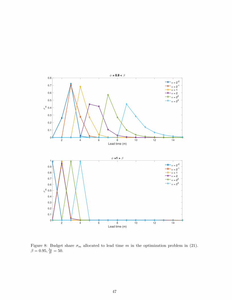
2 4 6 8 10 12 14

Lead time (m)

0

0.1

0.2

0.3

0.4

0.5

0.6

0.7

0.8

σm

φ = 0.9 < β

α = 2-2

α = 2-1

α = 1

α = 2

α = 22

α = 23

2 4 6 8 10 12 14

Lead time (m)

0

0.1

0.2

0.3

0.4

0.5

0.6

0.7

0.8

0.9

1

σm

φ =1 > β

α = 2-2

α = 2-1

α = 1

α = 2

α = 22

α = 23

Figure 8: Budget share σm allocated to lead time m in the optimization problem in (21).β = 0.95, λ0B = 50.

47