PREDICTION OF TSUNAMI PROPAGATION IN THE … · PREDICTION OF TSUNAMI PROPAGATION IN THE PEARL RIVER ESTUARY ... These models are MIKE21 model ... time step is assumed to be constant

PREDICTION OF TSUNAMI PROPAGATION IN THE PEARL RIVER ESTUARY

Sun J. S.,

Wai, O.W.H.*, Chau, K.T.

and Wong, R.H.C.

Department of Civil & Structural Engineering,

The Hong Kong Polytechnic University Hung Hom, Kowloon,

Hong Kong

*Corresponding author—Tel: (852) 27666025; Fax: (852) 23346389; email: [email protected]

ABSTRACT

Tsunamis entering into shallow water regions may become highly nonlinear and this may be due to the irregularity of sea bottom roughness relative to the water depth and the complex coastline geometry. The elliptic mild-slope equation is commonly used to predict the nonlinear wave propagation in shallow water regions but it requires huge amount of computer resources which may not be practical for tsunami propagation predictions. An efficient finite element approach has been adopted in the present project to resolve the nonlinear problem of wave transformation in near shore zones as well as to better conform the model grids to any complex coastline configurations. The efficient approach is based on the wave action conservation equation that takes into account of wave refraction-diffraction and energy dissipation due to bottom roughness. An operator splitting scheme is employed to solve the wave action conservation equation. Firstly, to increase numerical stability, the Eulerian-Lagrangian method is applied to solve the advection terms in the equation. The horizontal terms are then discretized by an implicit finite element method and, finally, the vertical terms are approximated by an implicit finite difference method. A nominal-time iteration method is used to efficiently solve the non-linear irrotational wave number equation for the wave direction. Over 6000 nine-node elements have been used to mesh the Pearl River estuary region. The boundary conditions are based on the results obtained from a simulation applied for a larger computation domain encompassing the entire South China Sea. The computed result provides a general picture of tsunami propagation in the desired region. Model validation and result verification, however, are necessary for any future prediction exercises. KEYWORDS: Tsunamis, shallow water regions, finite element approach, operator splitting scheme, PRe

Science of Tsunami Hazards, Vol. 28, No. 2, page 142 (2009)

1. INTRODUCTION Tsunami is a high impact low probability maritime hazard that poses a threat to the coastal communities worldwide. The M9.0 Asia Tsunami took place on Dec. 26, 2004 in the Northern part of Sumatra (Lay et al., 2005), the coast region were hit almost immediately by the largest waves with devastating effects. Most of the damages and death toll was caused by the unexpected attack of the tsunami flood waves. China has a very long stretch of coastline which is exposed to the open ocean. Tens of millions of citizens reside near the coast. Because of the recent rapid economic growth in China, there is a great momentum to push for the development of coastal areas. The coast of southeastern China may be affected by tsunamis generated by earthquakes in the northern part of the South China Sea and the Taiwan region. The study aims at acquiring a better understanding of any potentially hazard regions that are subject to the threat of tsunamis. Numerical modeling of tsunami serves a double purpose: it allows us to estimate the effects of events which have yet to happen, and it enables us to evaluate our understanding of past tsunami. There are a number of numerical models that are commonly used to simulate tsunami propagation. These models are MIKE21 model developed by the Danish Hydraulic Institute, the Delft3D model developed by Delft Hydraulics in Netherlands, the MOST (method of splitting tsunami) model developed at the University of Southern California in the United States of America (Titov and Synolakis, 1998); the COMCOT (Cornell multi-grid coupled tsunami model) model developed at Cornell University in the United States of America (Gica et al., 2007); TSUNAMI2 model developed at Tohoku University in Japan (Imamura, 1996) and so forth. In this study the three-dimensional wave model was introduced to simulate the tsunami propagation and wave run-up in the Pearl River estuary (Chen, 2001), which adopted an efficient finite element approach in the present project to resolve the nonlinear problem of wave transformation in near shore zones as well as to better conform the model grids to any complex coastline configurations. 2. TSUNAMI MODEL 2.1. Governing Equations The problem of gravity surface wave propagation with wave refraction and diffraction on non-uniform current and bottom friction can be described by the following equations. Irrotational wave number vector:

0)cos()sin(=

!

"!#

!

"!

y

K

x

K ww $$ (2.1)

Where K is the modified wave number;

w! is the wave propagation direction; and yx, are the Cartesian

coordinates. Dispersion relation:

2*2

4

1)tanh()]cos([ WhkgkUK cw !""=!"! ##$ (2.2)

where U is the current velocity;

c! is the current direction; k is the wave number; h is the water depth;

! is the wave angular frequency; g is the acceleration of gravity; and *W is the bottom friction coefficient,

3* ])sinh(

[3

4

khg

HfW w !

"= , wf is the wave friction factor.


For rough turbulent flow, a number of formulas have been proposed for the wave friction factor wf . Based

on 44 measured values of wf which are taken from seven sources, Soulsby (1997) proposed the following

equation for wf .

52.0

0

'

)(39.1 !=

z

Afw (2.3)

where !2/'

TUAw

= is the semi-orbital excursion; the roughness length 30/0 skz = ,

sk is the Nikurades

equivalent sand grain roughness; T is the wave period; and )sinh(

1

khT

HUw

!= .

Wave action conservation equation:

AWKcc

vAy

Kcc

uAxt

Aw

r

g

w

r

g!"=+

#

#++

#

#+

#

# *)]sin([)]cos([ $%

$%

(2.4)

where A is the wave action,2

2R

A!

= , !2

HR = , H is the wave height; u and v are the depth-averaged

current velocity in x and y directions; and t is the time. Wave eikonal equation:

])(2)(2[1 *

2

222

t

v

y

R

t

u

x

R

y

R

tv

x

R

tu

t

RW

t

R

RcckK

g !

!

!

!+

!

!

!

!+

!

!

!

!+

!

!

!

!+

!

!+

!

!"=

+ )]()([1

y

Rcc

yx

Rcc

xRccgg

g !

!

!

!+

!

!

!

!

]4

)()([1 2*

22R

W

y

Rv

x

Rvu

yy

Rvu

x

Ru

xRccg+

!

!+

!

!

!

!+

!

!+

!

!

!

!" (2.5)

in which c is the wave speed; and

gc is the wave group speed.

2.2. Boundary conditions The conditions at the boundaries enclosing the computational domain must be specified to completely define the problem. Two kinds of boundaries, namely, the incident wave boundaries and absorbing boundaries that absorb all wave energy arriving are considered. Generally, the incident wave boundary is the deepwater wave condition or the measured wave condition at the open boundary and the absorbing boundary is the land boundary. The wave energy arriving at absorbing boundaries from the fluid domain must be absorbed perfectly. The treatment of this kind of boundary is difficult in numerical modeling. The most commonly used method is the Sommerfeld radiation condition which can be written as:

0=+xxt

HCH

0=+ yyt HCH (2.6)


where

xC and yC are the phase speeds along the x and y directions, respectively. In the actual

computation, it is difficult to obtain the exact phase speeds and hence, the boundary can still reflect some wave energy. To eliminate the boundary reflections, a ‘sponge’ layer proposed by Larsen and Dancy (1983) is placed in front of an absorbing boundary to absorb the incoming wave energy. On the sponge layer, the wave height is divided by a factor, ( )yx,µ , after each step. The factor ( )yx,µ takes the following form after extending the one-dimensional form given by Larsen and Dancy (1983) to two dimensions (Li et al., 1999).

( )( )[ ]

!"#

<

$$%=

&%&%

dd

ddyx

s

s

dddd s

1

0ln22exp,

'µ (2.7)

in which d is the distance between the ‘sponge’ layer and the boundary; d! is the typical dimension of the elements;

sd is the sponge layer thickness, usually equal to one to two wave lengths and ! is a constant to

be specified. 2.3. Numerical Schemes The computation procedure starts from the seaward boundaries in which Eq. (2.1) is first solved for

w!

by assuming an initial value of the modified wave number, e.g. kK = . Using the values of w

! and K , Eq. (2.4) is then solved for the wave height. With the known values of the wave direction and wave height, the values K are updated using Eq. (2.5). The procedure is repeated until convergence is achieved. 2.3.1 Splitting of wave action equation To increase the numerical stability, an operator splitting method is applied to the wave action equation. The time integration of the wave action equation is performed in two sequential stages. That is, a time step is divided into two sub-steps in which the first step is for the advective terms and the second step is for the other terms. In the first sub-step, the advective term is solved for wave action. In general, numerical instability in wave propagation computations is mainly caused by the incorrect approximation of the advective term. To increase the numerical stability, an Eulerian-Lagrangian method is applied to discretize the advective term. The equation in this sub-step is given as:

0])sin[(])cos[(2

1

=!

!""++

!

!""++

#

$+

n

w

gn

w

gn

n

y

AK

ccv

x

AK

ccu

t

AA%

&%

& (2.8)

in which t! is time step. In the second sub-step, the other terms in the wave action equation are calculated using the implicit finite element method. The equation to be solved in this sub-step is:

1*2

1

12

1

12

1

1

)()sin()cos( ++

++

+

++

!"=!!+#

#!+!!+

#

#!+

$

" nn

w

gnn

w

gn

nn

AWKcc

vy

AKcc

ux

At

AA%

&%

& (2.9)


2.3.2 Spatial discretizations In the first sub-step, Eq. (2.8) is approximated by an explicit Eulerian-Lagrangian Method (ELM). The Eulerian-Lagrangian method has advantages over other commonly used numerical methods, such as the upwind method and the ADI method. The scheme was subsequently extended to three dimensions by Casulli and Cheng (1992). In the method, a fluid particle is assumed to arrive at a mesh node at the end of a time step, and the known value of a certain variable at the beginning of the time step is assumed to be constant over the time step. The position of the particle at the beginning of the time step may be obtained by backtracking and its value can be obtained through interpolation from the values at the surrounding mesh points. In this study, the Eulerian-Lagrangian method is employed to handle the advective term in the wave action equation. To obtain an Eulerian-Lagrangian approximation, a wave ray or the transport of the wave action from a point

ix over time is defined as follows.

w

gK

ccu

dt

dx!

"cos##+= , w

gK

ccv

dt

dy!

"sin##+= (2.10)

A particle that ends at a mesh node has a position at the beginning of the time step that can be obtained by assuming a constant wave velocity over the time step. This can be written as:

)cos( w

g

ip Kcc

utxx !"

##+#$%= , )sin( w

g

ip Kcc

vtyy !"

##+#$%= (2.11)

in which

px ,

py are the coordinates of a particle at a beginning position p ;

ix , iy are the coordinates of a

particle at node i . 2.3.3 Approximation of the other terms of the wave action equation by an implicit finite element method In the second step, the other terms in the wave action equation were calculated using the implicit finite element method (FEM). For accurate computations, the nine-node isoparameteric quadrilateral finite elements are employed in this model. The 2nd-order nine-node isoparametric shape functions are expressed as follows:

!!!

"

!!!

#

$

=%%

=%%+++

=++

=

9)1)(1(

8,...,5)1)(1)((2

1

4,...,1)1)(1)()((4

1

22

2222

jfor

jfor

jfor

jjjjjj

jjjj

j

&'

'&&'&&''&&''

&&''&&''

( (2.12)

in which ! is the interpolation function; ! and ! are the local coordinates.

Subdividing the domain of interest ! into finite elements and denoting a generic element by e! , the

dependent variables in wave action conservation equations are approximated within the elements as follows

!=

"nd

i

ii ff1

# (2.13)


where if is the values of any independent variable at the nodal points, nd is the number of nodes. The Galerkin's method with the use of integration by parts and Green's theorem are applied to Eq. (3.10). The following element matrix equations can be obtained.

[ ]{ } [ ]!"#

$%&

=+

+ 2

1

1n

i

n

iAA MD (2.14)

where T

NiAAAA ]...,[ ,21= , N is the number of nodes,

[ ]

}4)sin(3

)cos(211

1

{

)*()()()(

)()()(

e

l

e

jkl

e

lw

ge

jkl

e

lw

ge

jkl

e

jk

WSKcc

vS

Kcc

uSSt

M

e

D

!+!!+!+

!!+!+!"

#=

=

$%

$%

(2.15)

[ ] )11( )(

1

e

jk

M

e

St

M !"

=#=

(2.16)

!"## ddJSe

kj

e

jk $$= %%&

)(1 (2.17)

!"## ddPSe

lkj

e

jkl $$%

&&=)(2 (2.18)

!"## ddQSe

lkj

e

jkl $$%

&&=)(3 (2.19)

!!"

###=e

ddJS lkj

e

jkl $%&&&)(4 (2.20)

!

"

##

"

! $

$

$

$%

$

$

$

$=

jj

j

yyP (2.21)

!

"

##

"

! $

$

$

$+

$

$

$

$%=

jj

j

xxQ . (2.22)

Here, M is the total number of elements; and J is Jacobi matrix as given below

!!

""

#

#

#

#

#

#

#

#

=yx

yx

J (2.23)

2.3.4 Approximation of the wave number equation by an iteration method To solve the wave number equation (Eq. 2.1) for the wave direction, a direct discetization of this equation by either the finite element method or a finite difference method may end up with numerical instability in complex geometrical boundary situations. This problem is mainly due to the solution of a highly non-linear equation for


the entire computational domain in every time step. To increase stability, an iteration method is presented. A nominal (or fictitious) temporal derivative term is added to Eq. (2.1) and the spatial derivatives of the wave number are discretized by a finite node method (FNM) at each node. FNM is a mixture of the finite element method (FEM) and the finite difference method (FDM). The form of expression of the FNM is similar to that of the FEM and the basic solution process is the same as in FDM. Eq. (2.1) with the nominal temporal term is written as:

0)cos()sin(

'=

!

"!#

!

"!+

!

!

y

K

x

K

t

www $$$ (2.24)

where 't is the nominal time.

Using a finite node method, Equation (2.24) becomes:

}])sin([])cos([{)(1

)(

)('

1

)(

)('

0,

1

, !!==

+

"

"#$

"

"#%+=

ii M

e

n

i

e

jw

e

j

i

M

e

n

i

e

jw

e

j

i

n

iw

n

iw KxM

tK

yM

tKf &

'&

'&& (2.25)

in which iM is the number of elements around the i-th node; j! is the four-node isoparametric shape

function; )( 0Kf is a coefficient for improving numerical stability and speeding up convergence where

0

0

99.0)(

KKf

n

= ; 0

K is the deep water wave number. Note that the grid layouts for wave direction calculation

and the wave height calculation are the same. 2.4 Tsunami Simulations The main goal of the present project is to estimate tsunami propagation and wave run-up numerically in the Pearl River estuary (PRe) to gain better understanding of the tsunami risk in this region. The coast of southeastern China may be affected by tsunamis generated by earthquakes in the northern part of the South China Sea, therefore in this study; we used two bathymetry layouts to carry out more realistic simulations of the tsunami propagation. One layout covers the entire South China Sea (SCS) region obtained from the National Geophysical Data Centre ETOPO2 which consists of digital averaged land and sea floor elevations assembled from several uniformly gridded data bases with a grid spacing of 2 minutes of latitude by 2 minutes of longitude (about 3.6 km by 3.6 km in size). The PRe layout is obtained by combining the coastline data and non-uniform bathymetry grid data using software Surfer and ArcGIS. Figures 1 and 2 show the two-bathymetry layouts.

Figure 1 Bathymetry of SCS Figure 2 Bathymetry of PRe

Science of Tsunami Hazards, Vol. 28, No. 2, page 148 (2009

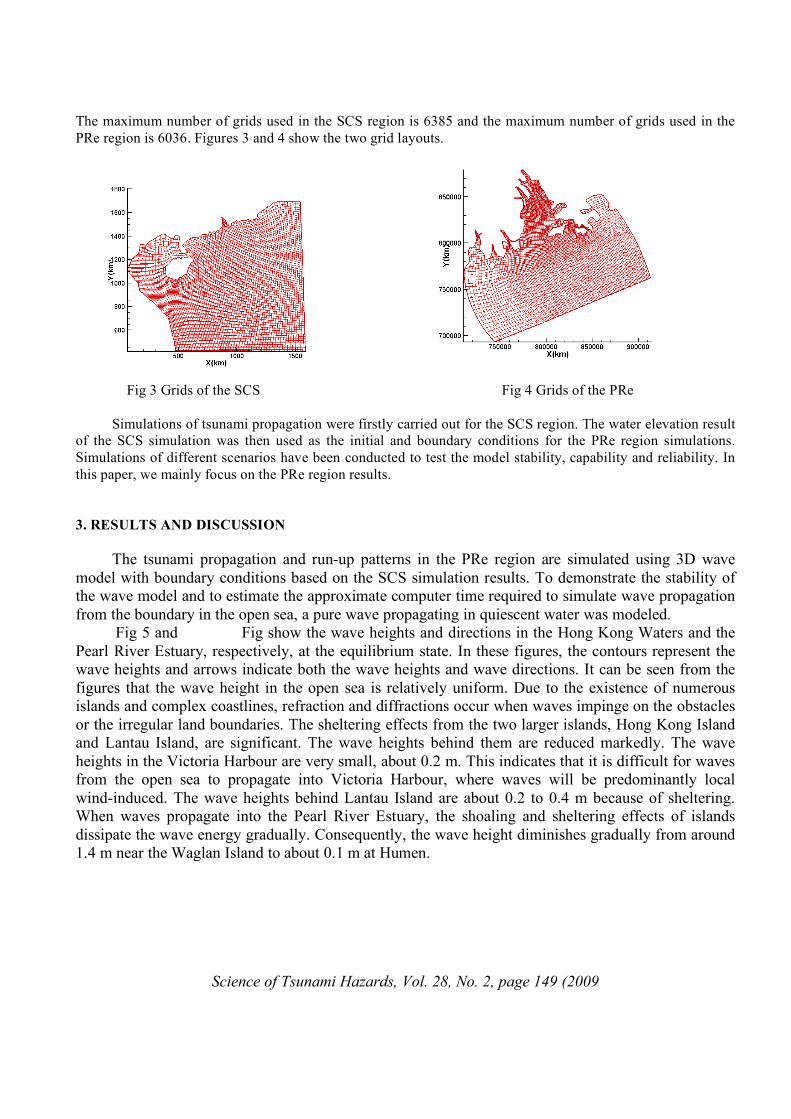
The maximum number of grids used in the SCS region is 6385 and the maximum number of grids used in the PRe region is 6036. Figures 3 and 4 show the two grid layouts.

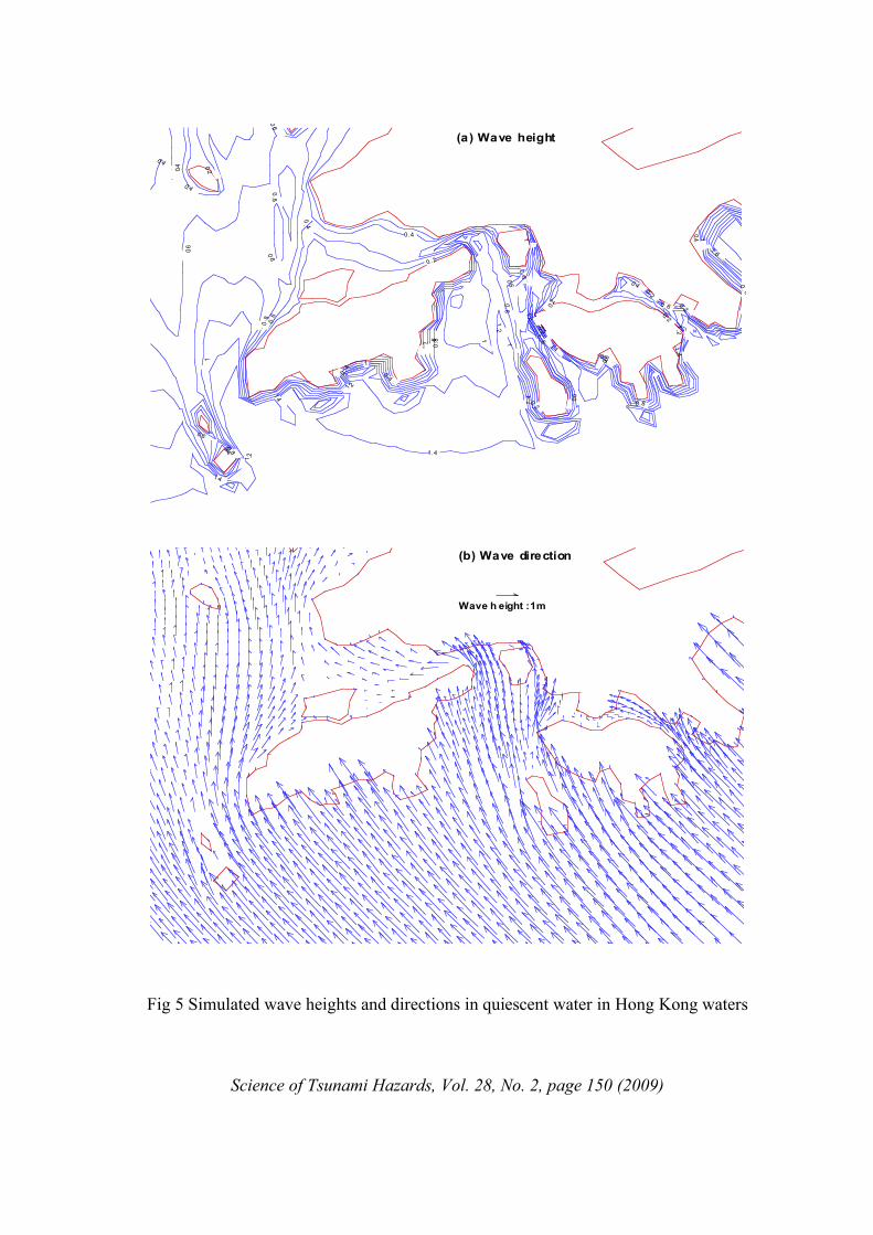
Fig 3 Grids of the SCS Fig 4 Grids of the PRe Simulations of tsunami propagation were firstly carried out for the SCS region. The water elevation result of the SCS simulation was then used as the initial and boundary conditions for the PRe region simulations. Simulations of different scenarios have been conducted to test the model stability, capability and reliability. In this paper, we mainly focus on the PRe region results. 3. RESULTS AND DISCUSSION The tsunami propagation and run-up patterns in the PRe region are simulated using 3D wave model with boundary conditions based on the SCS simulation results. To demonstrate the stability of the wave model and to estimate the approximate computer time required to simulate wave propagation from the boundary in the open sea, a pure wave propagating in quiescent water was modeled. Fig 5 and Fig show the wave heights and directions in the Hong Kong Waters and the Pearl River Estuary, respectively, at the equilibrium state. In these figures, the contours represent the wave heights and arrows indicate both the wave heights and wave directions. It can be seen from the figures that the wave height in the open sea is relatively uniform. Due to the existence of numerous islands and complex coastlines, refraction and diffractions occur when waves impinge on the obstacles or the irregular land boundaries. The sheltering effects from the two larger islands, Hong Kong Island and Lantau Island, are significant. The wave heights behind them are reduced markedly. The wave heights in the Victoria Harbour are very small, about 0.2 m. This indicates that it is difficult for waves from the open sea to propagate into Victoria Harbour, where waves will be predominantly local wind-induced. The wave heights behind Lantau Island are about 0.2 to 0.4 m because of sheltering. When waves propagate into the Pearl River Estuary, the shoaling and sheltering effects of islands dissipate the wave energy gradually. Consequently, the wave height diminishes gradually from around 1.4 m near the Waglan Island to about 0.1 m at Humen.

Science of Tsunami Hazards, Vol. 28, No. 2, page 149 (2009

0 .2

0.2

0. 20. 2

0.2

0. 2

0. 2

0 .2

0.2

0 .2

0. 4

0. 4

0. 4

0 .4

0. 4

0. 4

0 .4

0 .4

0 .4

0.4

4

0.4

0.4

0.6

0.6

0.6

0.6

0. 6

0.6

0 .6

0 .6

0.6

0.6

0. 8

0. 8

0.8

0.8

0. 8

0 .8

0. 8

0.8

1

1

1

1

1

1

1

1 .2

1 .2

1.2

1 .2

1.2

1 .4

1.4

1.4

1. 4 1.4

1.4

1. 6

1 .6

.8

1 .4

(a) Wave height

(b) Wave direction

Wave h eight :1m

Fig 5 Simulated wave heights and directions in quiescent water in Hong Kong waters


wave h eight: 1m

( b) W ave direction

0.2

0.2

0.2

0.2 0 .2

0.2

0.2

0.2

0. 20.2

0.2

0.2

0. 20. 2

0 .2

0. 2

0 .2

0 .4

0.4

0.4

0. 4

0. 4

0. 4

0 .4

0.4

0. 4

0. 4

0 .4

0. 4

0.4

0.4

0.4

0.4

0.6

0 .6

0.6

0.6

0.6

0 .6

0.6

0.6

0. 6

0 .6

0.6

0.6

0. 6

0.6

0.6

0 .8

0.8

0. 8

0.8

0.8

0.8

0.8

0 .8

0.8

0.8

0.

0.8

1

1

1

1

1

1

1

1

1

1

1.2

1.2

1. 2

1. 2

1. 2 1.2

1 .2

1 .2

1.4

1.4

1.4

1.4

1. 4

1.4

1 .4

1.4

1 .4

1.4

1.6

1. 6

1. 8

1.4

1 .2

1

0. 8

0.6

1.4

( a) W ave height

Fig 6 Simulated wave heights and directions in quiescent water in Pre


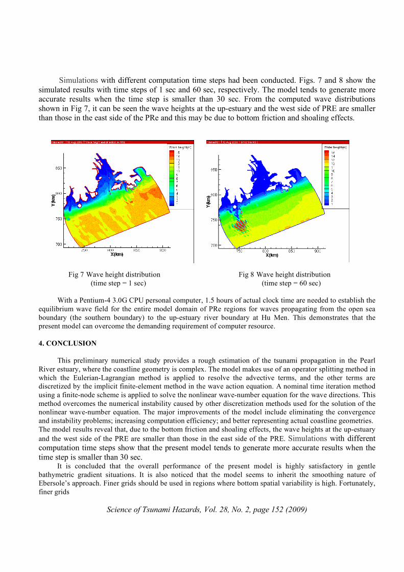
Simulations with different computation time steps had been conducted. Figs. 7 and 8 show the simulated results with time steps of 1 sec and 60 sec, respectively. The model tends to generate more accurate results when the time step is smaller than 30 sec. From the computed wave distributions shown in Fig 7, it can be seen the wave heights at the up-estuary and the west side of PRE are smaller than those in the east side of the PRe and this may be due to bottom friction and shoaling effects.

Fig 7 Wave height distribution Fig 8 Wave height distribution (time step = 1 sec) (time step = 60 sec)

With a Pentium-4 3.0G CPU personal computer, 1.5 hours of actual clock time are needed to establish the equilibrium wave field for the entire model domain of PRe regions for waves propagating from the open sea boundary (the southern boundary) to the up-estuary river boundary at Hu Men. This demonstrates that the present model can overcome the demanding requirement of computer resource. 4. CONCLUSION This preliminary numerical study provides a rough estimation of the tsunami propagation in the Pearl River estuary, where the coastline geometry is complex. The model makes use of an operator splitting method in which the Eulerian-Lagrangian method is applied to resolve the advective terms, and the other terms are discretized by the implicit finite-element method in the wave action equation. A nominal time iteration method using a finite-node scheme is applied to solve the nonlinear wave-number equation for the wave directions. This method overcomes the numerical instability caused by other discretization methods used for the solution of the nonlinear wave-number equation. The major improvements of the model include eliminating the convergence and instability problems; increasing computation efficiency; and better representing actual coastline geometries. The model results reveal that, due to the bottom friction and shoaling effects, the wave heights at the up-estuary and the west side of the PRE are smaller than those in the east side of the PRE. Simulations with different computation time steps show that the present model tends to generate more accurate results when the time step is smaller than 30 sec. It is concluded that the overall performance of the present model is highly satisfactory in gentle bathymetric gradient situations. It is also noticed that the model seems to inherit the smoothing nature of Ebersole’s approach. Finer grids should be used in regions where bottom spatial variability is high. Fortunately, finer grids


can be easily established at any desired regions in the model domain with the unstructural finite-element scheme equipped in the model. Model validation and result verification, however, are necessary for any future prediction exercises. ACKNOWLEDGEMENT This research was supported separately by two Central Research Grants of The Hong Kong Polytechnic University (Account Nos.: 87K1 and G-U198.) REFERENCES Casulli, V. and Cheng, R.T. (1992). SEMIIMPLICIT FINITE-DIFFERENCE METHODS FOR 3-DIMENSIONAL SHALLOW-WATER FLOW. International Journal for Numerical Methods in Fluids 15, 629-648. Chen, Y. (2001). Sediment transport by waves and currents in the Pearl River Estuary. Ph.D. thesis, Department of Civil and Structural Engineering, The Hong Kong Polytechnic University, Hong Kong. Gica, E., Teng, M.H., Liu, P.L.F., Titov, V. and Zhou, H.Q. (2007). Sensitivity analysis of source parameters for earthquake-generated distant tsunamis. Journal of Waterway Port Coastal and Ocean Engineering-ASCE 133, 429-441. Larsen, J. and Dancy, H. (1983). Open Boundary in short wave simulation – a new approach. Coastal Eng7: 3, 285-297 Lay, T. et al., (2005). The great Sumatra-Andaman earthquake of 26 December 2004. Science 308, 1127-1133. Imamura, F. (1996). Review of tsunami simulation with a finite difference method. Long Wave Runup Models. World Scientific Publishing Li, B.G., Xie, Q.C. and Xia, X.M. (1999). Particle size distribution in the turbidity maximum and its responding to the tidal flow in Jiao Jiang Estuary. Journal of Sediment Research 1, 18-26. Soulsby, R.L. (1997). Dynamics of Marine Sands. A Manual for Practical Applications. Titov, V.V. and Synolakis, C.E. (1998). Numerical modeling of tidal wave run-up. Journal of Waterway Port Coastal and Ocean Engineering-ASCE 124, 157-171.


PREDICTION OF TSUNAMI PROPAGATION IN THE … · PREDICTION OF TSUNAMI PROPAGATION IN THE PEARL RIVER ESTUARY ... These models are MIKE21 model ... time step is assumed to be constant

Documents