1. Report No. 2. Government Accession No. FHWATX-77-23-l 4. Title and Subtitle PREDICTION OF TEMPERATURE AND STRESSES IN HIGHWAY BRIDGES BY A NUMERICAL PROCEDURE USING DAILY WEATHER REPORTS 7. Authorl s) Thaksin Thepchatri, C. Philip Johnson, and Hudson Matlock 9. Performing Orgoni zation Name and Address Center for Highway Research The University of Texas at Austin Austin, Texas 78712 12. Sponsoring Agency Name and Address Texas State Department of Highways and Public Transportation; Transportation Planning Division P.O. Box 5051 Austin, Texas 78763 15. Supplementary Notes TECHNICAL REPORT ST ANDARD TIT L E PAG E 3. Recipient's Catalog No. 5. Report Date February 1977 6. Performing Organi zation Code 8. Performing Orgoni zation Report No. Research Report Number 23-1 10. Work Unit No. 11. Contract or Gront No. Research Study 3-5-74-23 13. Type of Report and Period Covered Interim 14. Sponsoring Agency Code Work done in cooperation with the Department of Transportation, Federal Highway Administration. Research Study Title: "Temperature Induced Stresses in Highway Bridges by Finite Element Analysis and Field Tests" 16. Abstract This research focused on the development of computational procedures for the prediction of the transient bridge temperature distribution due to daily variations of the environment such as solar radiation, ambient air temperature, and wind speed. The temperature distribution is assumed to be constant along the center- line of the bridge but can vary arbitrarily over its cross section. The finite element method was used for the two-dimensional heat flow analysis. Temperature stresses, however, are computed from elastic beam theory. In this work a computer program, TSAP, which included the heat flow and thermal stress analysis in a complete system was developed. The environmental data required for input are the solar radiation intensity, ambient air temperature and wind speed. Daily solar radiation intensity is available through the U.S. Weather Bureau at selected locations while air temperature and wind speed can be obtained from local newspapers. This program provides a versatile and economical method for predicting bridge temperature distributions and the ensuing thermal stresses caused by daily environmental changes. Various types of highway bridge cross-sections can be considered. In this work, three bridge types are considered: (1) a post- tensioned concrete slab bridge, (2) a composite precast pretensioned bridge, and (3) a composite steel bridge. Specific attention was given to the extreme summer and winter climatic conditions representative of the city of Austin, Texas. 17. Key Words prediction, temperature, stresses, bridges, procedure, weather, model, finite element, elastic beam theory 18. Distribution Statement No restrictions. This document is available to the public through the National Technical Information Service, Springfield, Virginia 22161. 19. Security Clauil. (01 this report) 20. Security Ctaulf. (of thi s page) 21. No. of Pages 22. Pri ce Unclassified Unclas s ified 165 Form DOT F 1700.7 (e-611)

Welcome message from author
This document is posted to help you gain knowledge. Please leave a comment to let me know what you think about it! Share it to your friends and learn new things together.
Transcript

1. Report No. 2. Government Accession No.
FHWATX-77-23-l
4. Title and Subtitle
PREDICTION OF TEMPERATURE AND STRESSES IN HIGHWAY BRIDGES BY A NUMERICAL PROCEDURE USING DAILY WEATHER REPORTS 7. Authorl s)
Thaksin Thepchatri, C. Philip Johnson, and Hudson Matlock 9. Performing Orgoni zation Name and Address
Center for Highway Research The University of Texas at Austin Austin, Texas 78712
~------------------------------------------------------~ 12. Sponsoring Agency Name and Address
Texas State Department of Highways and Public Transportation; Transportation Planning Division
P.O. Box 5051 Austin, Texas 78763 15. Supplementary Notes
TECHNICAL REPORT ST ANDARD TIT L E PAG E
3. Recipient's Catalog No.
5. Report Date
February 1977 6. Performing Organi zation Code
8. Performing Orgoni zation Report No.
Research Report Number 23-1
10. Work Unit No.
11. Contract or Gront No.
Research Study 3-5-74-23 13. Type of Report and Period Covered
Interim
14. Sponsoring Agency Code
Work done in cooperation with the Department of Transportation, Federal Highway Administration. Research Study Title: "Temperature Induced Stresses in Highway Bridges by Finite Element Analysis and Field Tests" 16. Abstract
This research focused on the development of computational procedures for the prediction of the transient bridge temperature distribution due to daily variations of the environment such as solar radiation, ambient air temperature, and wind speed. The temperature distribution is assumed to be constant along the centerline of the bridge but can vary arbitrarily over its cross section. The finite element method was used for the two-dimensional heat flow analysis. Temperature stresses, however, are computed from elastic beam theory.
In this work a computer program, TSAP, which included the heat flow and thermal stress analysis in a complete system was developed. The environmental data required for input are the solar radiation intensity, ambient air temperature and wind speed. Daily solar radiation intensity is available through the U.S. Weather Bureau at selected locations while air temperature and wind speed can be obtained from local newspapers. This program provides a versatile and economical method for predicting bridge temperature distributions and the ensuing thermal stresses caused by daily environmental changes. Various types of highway bridge cross-sections can be considered. In this work, three bridge types are considered: (1) a posttensioned concrete slab bridge, (2) a composite precast pretensioned bridge, and (3) a composite steel bridge. Specific attention was given to the extreme summer and winter climatic conditions representative of the city of Austin, Texas.
17. Key Words
prediction, temperature, stresses, bridges, procedure, weather, model, finite element, elastic beam theory
18. Distribution Statement
No restrictions. This document is available to the public through the National Technical Information Service, Springfield, Virginia 22161.
19. Security Clauil. (01 this report) 20. Security Ctaulf. (of thi s page) 21. No. of Pages 22. Pri ce
Unclassified Unclas s ified 165
Form DOT F 1700.7 (e-611)
PREDICTION OF TEMPERATURE AND STRESSES IN HIGHWAY BRIDGES BY A NUMERICAL PROCEDURE USING
DAILY WEATHER REPORTS
by
Thaksin Thepchatri C. Philip Johnson
Hudson Matlock
Research Report Number 23-1
Temperature Induced Stresses in Highway Bridges by Finite Element Analysis and Field Tests
Research Project 3-5-74-23
conducted for
Texas State Department of Highways and Public Transportation
in cooperation with the U. S. Department of Transportation
Federal Highway Administration
by the
CENTER FOR HIGHWAY RESEARCH
THE UNIVERSITY OF TEXAS AT AUSTIN·
February 1977

The contents of this report reflect the views of the authors, who are responsible for the facts and the accuracy of the data presented herein. The contents do not necessarily reflect the official views or policies of the Federal Highway Administration. This report does not constitute a standard, specification, or regulation.
ii

PREFACE
Computational procedures for predicting temperature and stresses in
highway bridges due to daily environmental changes are presented. A two
dimensional finite model is used for predicting the temperature distribution
while elastic beam theory is used for predicting the bridge stresses. The
environmental data required in the analysis are available from daily weather
reports.
Program TSAP, which included the subject procedures in a complete system,
was used to predict bridge temperature and stress distributions caused by the
climatic conditions representative of the city of Austin, Texas. Several
individuals have made contributions in this research. With regard to this
project special thanks are due to John Panak, Kenneth M. Will, and Atalay
Yargicoglu. In addition, thanks are due to Nancy L. Pierce and the members of
the staff of the Center for Highway Research for their assistance in producing
this report.
iii


ABSTRACT
This research focused on the development of computational procedures
for the prediction of the transient bridge temperature distribution due
to daily variations of the environment such as solar radiation, ambient
air temperature, and wind speed. The temperature distribution is assumed
to be constant along the center-line of the bridge but can vary arbitrarily
over its cross section. The finite element method was used for the two
dimensional heat flow analysis. Temperature stresses, however, are computed
from elastic beam theory.
In this work a computer program, TSAP, which included the heat flow
and thermal stress analysis in a complete system was developed. The
environmental data required for input are the solar radiation intensity,
ambient air temperature and wind speed. Daily solar radiation intensity
is available through the U.S. Weather Bureau at selected locations while
air temperature and wind speed can be obtained from local newspapers.
This program provides a versatile and economical method for predicting
bridge temperature distributions and the ensuing thermal stresses caused
by daily environmental changes. Various types of highway bridge cross
sections can be considered. In this work, three bridge types are considered:
1) a post-tensioned concrete slab bridge, 2) a composite precast pretensioned
bridge, and 3) a composite steel bridge. Specific attention was given to
the extreme summer and winter climatic conditions representative of the city
of Austin, Texas.
v

SUMMARY
A computational procedure for the prediction of temperature induced
stresses in highway bridges due to daily changes in temperature has been
developed. The procedure has been implemented into a computer program,
TSAP, which is able to predict both the temperature distribution and the
temperature induced stresses for a variety of bridge types. This work
is of particular significance because the important environmental data
required in the analysis (such as solar radiation, ambient air temperature
and wind speed) are available from daily weather reports. A two-dimensional
finite model is used for predicting the temperature distribution while
ordinary beam theory is used for predicting the bridge movements and stresses
due to temperature changes. Outgoing (long-wave) radiation, which has not
been considered in the past, was included in the finite element temperature
model, thus allowing for a continuous temperature prediction over a given
period of days and nights.
This research indicates that the amplitude and form of the temperature
gradient are mainly functions of the intensity of the solar radiation,
ambient air temperature and wind speed. The most extreme environmental
conditions for Austin, Texas, were found to take place on a clear night
followed by a clear day with a large range of air temperature. The shape
and depth of the bridge cross-section and its material thermal properties
such as absorptivity, emissivity, and conductivity, are also significant
factors. For example, due to the low thermal conductivity of concrete,
the nonlinearity of the temperature distribution in deep concrete structures
was found to be considerable greater than that experienced in composite
steel bridges. In addition to the nonlinear form of the temperature gradient,
temperature stresses also arise from the form of statical indeterminancy
of the bridge. This study indicates that temperature induced stresses in
any statically indeterminate bridge will be bounded by the stresses computed
from a one- and two-span case.
vii

viii
Results for three bridge types subjected to environmental conditions
representative of Austin, Texas, are presented. In general, it was found
that thermal deflections are small. Thermal stresses, however, appear to
be significant. For the weather conditions considered, temperature induced
tensile stresses in a prestressed concrete slab bridge and a precast
prestressed I-Beam were found to be in the order of 60 to 80 percent
respectively of the cracking stress of concrete suggested by the AASHTO
Specifications. Compressive stresses as high as 40 percent of the allowable
compressive strength were predicted in a prismatic thick slab having a depth
of 17 inches. For a composite steel-concrete bridge, on the other hand,
temperature stresses were approximately 10 percent of the design dead and
live load stresses.

IMPLEMENTATION
As a result of this research a computer program, TSAP (Temperature
and Stress Analysis Program), has been developed to form a complete system
for predicting temperature behaviors of highway bridges due to daily changes
of temperature. Based on the favorable comparisons between the predicted
and measured results, the proposed method offers an excellent opportunity
to determine bridge types and environmental conditions for which temperature
effects may be severe.
A user's guide, the program listing, and example problems will be
contained in the final report of project No. 3-5-74-23. This program has
been recently adapted to the computer facilities of the Texas State
Department of Highways and Public Transportation. Since the method used is
based on a two-dimensional model for predicting the temperature distribution
and ordinary beam theory for the stress analysis, the program is relatively
easy to use. Environmental data is available through regular Weather
Bureau Reports while material thermal properties may be obtained from one
of the handbooks on concrete engineering. In this study three types of
highway bridges subjected to climatic changes found in Austin, Texas, were
considered. These bridges were analyzed for several environmental conditions
representative of both summer and winter conditions.
This study has demonstrated the feasibility and validity of analytically
predicting the structural response of bridge superstructures subjected to
daily atmospheric variations. Typical magnitudes of temperature induced
stresses for three bridge types have been established. Since solar radiation
levels vary considerably with altitude, air pollution and latitude,
additional studies were undertaken for other locations in the State of Texas.
The results of that study will be summarized in the final report mentioned
above. The adaptation of TSAP to the Highway Department computer facilities
will allow the department engineers to directly determine the temperature
induced stresses for other bridge types in different locations in the State
of Texas.
ix

TABLE OF CONTENTS
PREFACE
ABSTRACT
SUMMARY . . . . IMPLEMENTATION . . . . . . . . . . . LIS T OF TABLES . . . . . . LIST OF FIGURES . . . . . . . . . . .
CHAPTER 1. INTRODUCTION. . . . .. . 1.1 General
1.2 Literature Review
1.3 Objective and Scope of the Study.
CHAPTER 2.
2.1
2.2
THE NEED AND THE APPROACH
The Need . •
The-Approach.
CHAPTER 3. ENVIRONMENTAL VARIABLES INFLUENCING BRIDGE TEMPERATURE
iii
v
vii
ix
xv
xvii
1
1
2
5
9
9
10
AND HEAT FLOW CONDITIONS • 13
3.1 Introduction. • . . . . 13
3.2 Environmental Variables 13
3.2.1 Solar Radiation.
3.2.2 Air Temperature
3.2.2 Wind Speed
3.3 Heat Flow Conditions
3.3.1 Heat Flow by Radiation
3.3.2 Heat Flow by Convection.
3.3.3 Heat Flow by Conduction.
CHAPTER 4. MATHEMATICAL MODELS
4.1
4.2
Introduction • • .
Bridge Temperature Prediction
xi
14
18
20
23
23
26
27
31
31
31

xii
4.2.1 One-Dimensional Model for Predicting the Temperature Distribution • • • . • • . •
4.2.2 Two Dimensional Model for Predicting the Temperature Distribution
4.3 Thermal Stress Analysis ••••
Page
31
39
46
4.3.1 Thermal Stress Analysis using the One-Dimensional Temperature Distribution Model • • • . • • . • •• 49
4.3.2 Thermal Stress Analysis using the Two-Dimensional Temperature Distribution Model • • • • 52
4.3.3 Applications of the Method to Different Types of Bridge Geometry • • • • • . . . . . . . 53
CHAPTER 5.
5.1
VERIFICATIONS OF THE MATHEMATICAL MODELS
Introduction • • • • •
57
57
57
61
63
69
5.2 Temperature Prediction by the One-Dimensional Model
5.3 Temperature Prediction by the Two-Dimensional Model
5.3.1 Temperature Prediction on August 8, 1967
5.3.2 Temperature Prediction on December 11, 1967 •
CHAPTER 6. THERMAL EFFECTS IN PRESTRESSED CONCRETE SLAB BRIDGE
6.1 Introduction . . • • • •
6.2 Temperature Effects in a Prismatic Concrete Slab Bridge
6.2.1 Sensitivity Analysis of the Model ••
6.2.2 A Study on Initial Conditions
6.2.3 A Study on Summer Conditions
6.2.4 A Study on Winter Conditions
6.2.5 Effects of Interior Supports on Temperature Induced Stresses . • • • • . • . . . • • •
6.2.6 Effects of Longitudinal Restraining Forces on Temperature Induced Stresses . . • • •
6.2.7 A Study on Polynomial Interpolation •••
6.3 Temperature Effects in a Non-Prismatic Concrete Slab Bridge • • • • • • .
6.4 Summary
77
77
77
79
82
86
86
89
94
94
96
100

CHAPTER 7. THERMAL EFFECTS IN COMPOSITE BRIDGES
7.1
7.2
Introduction • • • . . • • . .
Composite Precast Pretensioned Bridge
7.2.1 Temperature Effects on a Warm Sunny Day
7.2.2 Temperature Effects on a Cold Sunny Day
7.2.3 General Remarks
7.3 Composite Steel Bridge.
7.4
7.5
CHAPTER 8.
8.1
8.2
8.3
7.3.1 Temperature Effects on a Warm Sunny Day
7.3.2 Temperature Effects on a Cold Sunny Day
Interface Forces . . . . . . . . . . . Pedestrian Overpass (Narrow Structure) . . . .
SUMMARY, CONCLUSIONS AND RECOMMENDATIONS.
Summary
Conclusions
Recommendations
. .
.
APPENDIX A. COEFFICIENTS OF MATRICES FOR A PLANE TRIANGULAR ELEMENT •..................•
APPENDIX B. EFFECT OF PRESTRESSING STEEL ON END FORCES
. . .
xiii
Page 103
103
104
104
108
110
110
III
114
117
120
127
127
128
129
133
139
BIBLIOGRAPHY . . • • • . • • • . . . . . . • . • . . . • . • . . •• 141


Table
3.1
3.2
3.3
5.1
5.2
LIST OF TABLES
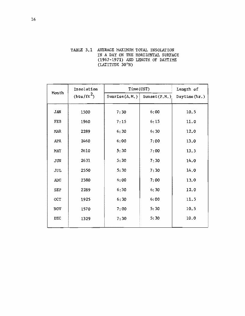
Average maximum total insolation in a day on the horizontal surface (1967-1971) and length of daytime (Latitude 30 0 N) • • . . . . • • • • •
Normals, means and extremes (Latitude 30 0 l8'N)
Values of emissivity and absorptivity
Average values of concrete thermal properties and pertinent data • . . .
Field test on August 8, 1967
16
21
24
60
65
5.3 Relevant data for thermal analysis on August 8, 1967 66
5.4 Field test on December 10-11, 1967 72
5.5 Data on December 10-11, 1967 73
6.1 Selected average values for the sensitivity analysis (August) ....... . . . . . . . . . . . . 80
6.2 The effects of a 10% increase in one variable at a time on temperatures and stresses in a three equal span concrete slab bridge (August) •....•.......•.•... 81
xv


Figure
1.1
3.1
3.2
3.3
3.4
3.5
4.1
4.2
4.3
4.4
4.5
4.6
4.7
4.8
5.1
5.2
5.3
5.4
5.5
5.6
5.7
5.8
5.9
LIST OF FIGURES
Typical highway bridge cross sections
Hourly distributions of solar radiation intensity for a clear day (Latitude 30 0 N) ... . . . . . . . . . . . .
Hourly distributions of air temperature (Austin, Texas).
Average maximum and minimum air temperatures (Austin, Texas) .•••.•.•••••
Variation of convective film coefficient with wind speed (Ref 51) . • • • • . . . • • . . • • • .
Variation of thermal conductivity with density (Ref 5)
A typical slab cross section showing nodal point numbering . • . • • • • • • • • • .
A typical slab cross section showing equations used in calculating temperatures . . •
A typical triangular element
A typical quadrilateral element
Spring system analogy to the thermal stress calculation. •
One-dimensional model shoWing the method of calculating temperature forces . • • . • • • • . . • . • . . . • . . .
Two-dimensional model showing the method of calculating temperature forces . • • . . . . .
Elevation views of highway bridges
Three-span post-tensioned concrete slab bridge
Measured air temperature and solar radiation intensity
Measured and predicted surface temperatures
40' - 0" concret slab and girder bridge
Bridge section and idealization
Temperature distributions at the center of the section (Aug. 8, 1967) . . . . • . . . . . . . .
Temperatures and vertical deflection vs. time (Aug. 8, 1967) ........... .
Temperature induced stresses
Temperature distributions at the center of the section (Dec. 11, 1967) ...... ..... . .. .
xvii
Page
7
17
19
22
28
28
35
37
44
44
48
50
50
54
58
59
59
62
64
67
70
71
74
xviii
Figure
5.10
6.1
6.2
6.3
6.4
6.5
6.6
6.7
6.8
6.9
6.10
6.11
6.12
7.1
7.2
7.3
7.4
7.5
7.6
7.7
7.8
7.9
Temperatures and vertical deflection vs. time (Dec. 11, 1967) •..••.•••.•••
160 I - 0" continuous concrete slab bridge .
Effect of starting conditions on temperature and stress distributions (August) • • . . • • . • . • • • •
Effect of the environmental repetition on temperature and stress distributions • • • • • • . • • • • • . . . • • • •
Temperature and stress distributions (summer condit.ions) •••••••.•.•.••••
Plots of temperatures for a clear day and night
Temperature and stress distributions (winter conditions) . . . · · · · · · · · · · · · Temperature induced stresses for a one-, two-, and three-span bridge (August) · · · · · · · Temperature induced stresses for a one-, two-, and three-span bridge (January) · · · Representative polynomial interpolations for temperature distributions . . · · · · · · · · · · · · · · · Fourth order polynomial components representing temperature and stress distributions • • . . . .
Prestressed non-prismatic concrete slab and the
· ·
idealization . • • • . • • . • • • • •
Temperature induced stresses . • •
· ·
Typical interior girder idealization of a composite precast pretensioned bridge (Texas standard type B-beam).
Temperature and stress distributions (August)
Temperature and stress distributions at the section of synnnetry. /I • • /I /I /I /I /I /I /I • /I /I • /I /I /I /I /I /I
Temperature and stress distributions (January) • • • .
Typical interior girder idealization of a composite steel bridge /I • • /I /I • /I /I /I • • , /I /I • II /I /I /I /I /I
Temperature and stress distributions at the section of symmetry (August) · · · · · · · · · · · · · , · · Temperature and stress distributions at the section of symmetry (August) · · · · · · · · · · · · · · · · Temperature and stress distributions at the section of symmetry (January) · · · · · · · · · · · · · · · · · · Variation of shear at the ends of a composite beam for a temperature difference of 2l.5°F (11.9°C) between the slab and beam (Ref 5) ••••••••••• . • •
· ·
·
·
76
78
83
85
87
88
90
91
93
95
97
98
99
105
106
107
109
112
113
115
116
118
Figure
7.10
7.11
7.12
7.13
7.14
A.1
Interface forces near the slab end caused by a temperature differential • . • • • . .
Pedestrian overpass (Austin, Texas)
Temperature variations with time on March 14, 1975
Comparisons of measured and predicted slope change vs. time for the pedestrian overpass . . . . . . • . .
Longitudinal temperature induced stresses vs. time at the center section over the interior support •
A typical triangular element . .
xix
119
121
123
125
126
134
CHAPTER 1. INTRODUCTION
1.1 General
It has been recognized for a long time that bridge superstructures
exposed to environmental conditions exhibit considerable structural
response. Temperature effects in bridges are affected by both daily and
seasonal temperature changes. For a statically determinate structure, the
seasonal change will not lead to temperature induced stresses. This
temperature change, however, causes large overall expansion and contraction.
Daily fluctuations of temperature, on the other hand, result in temperature
gradients through the depth of the bridge which in turn induce high internal
stresses.
Although current bridge specifications (41)* have provisions concerning
thermal movements in highway bridges, they do not have specific statements
in regard to temperature induced stresses. It is well known that no in
duced stresses are produced in a single span statically determinate bridge
if the temperature distribution has either a uniform or linear form. How
ever, experiences from field measurements in various types of bridges (20,
48,58) indicate that temperature distributions over the depth of the bridge
are nonlinear. The nonlinear temperature distribution is a source of
induced stresses even if the bridge is statically determinate. For inde
terminate structures, the structural response under temperature differentials
is believed to be more severe. This is true since additional internal
stresses are induced due to the flexural restraint caused by interior
supports. Hence, in general, the temperature stresses are attributed to
two principal factors: 1) the nonlinear form of the temperature gradient
through the depth of the bridge, and 2) to the form of statical indeter
minacy of the bridge.
* Numbers in parentheses refer to references in the Bibliography.
1

2
Research which has been performed on the subject to date indicates
that the amplitude and form of the temperature gradient are mainly functions
of the intensity of the solar radiation, ambient air temperature and wind
speed. The shape and depth of the bridge cross-section and its material
properties are also the significant factors. For example, due to the low
thermal conductivity of concrete, the nonlinearity of the temperature
distribution in concrete structures is found to be considerably greater
than that experienced in steel structures. Consequently, high stresses can
be induced in deep concrete bridges. These stresses, under particular con
dition, are additive to stresses caused by dead load and live loads; thus
increasing the magnitude of the final stresses. Cracks in an exposed
building structure due to high temperature stresses were reported by Meenan
(38). He found that temperature differentials could cause small vertical
cracks in the beam web in the vicinity of the intermediate support. The
structure was a two-span, continuous post-tensioned concrete beam.
Temperature induced stresses are generally ignored in the design pro
cess. Thermal movements together with creep and shrinkage, on the other
hand, are considered in the design by means of expansion joints (17). A
survey of bridge specifications by Zuk (59) has shown that Germany, Austria,
Sweden and Japan are the only countries with a thermal induced stress pro
vision in their specifications. During the past two decades, temperature
effects in highway bridges have been studied by several researchers in an
effort to assess the magnitudes of temperature stresses caused by environ
mental changes. In the following, some of the pertinent developments will
be presented.
1.2 Literature Review
Narouka, Hirai and Yamaguti (40) performed temperature tests on the
interior of a composite steel bridge in Japan in 1955. The results of the
tests showed that temperature distributions over the thickness of the con
crete slab were nonlinear. The maximum temperature gradient in the slab
was about 16°F. The maximum temperature differential between the top and
bottom flanges of the steel girder, on the other hand, was only 5°F.

3
In 1957, Barber (1) presented a formula to estimate the maximum pave
ment surface temperature. The model took into account the relationship
between pavement temperature, air temperature, wind speed, solar radiation
intensity and the thermal properties of the pavement materials.
Zuk (57) in 1961 developed a rigorous method for computing thermal
stresses and deflections in a statically determinate composite bridge.
Equations were given explicitly for estimating stresses and strains due to
various linear thermal gradients over the bridge cross section.
In 1963, Liu and Zuk (35) extended Zuk's earlier work (57) to study
temperature effects in simply supported prestressed concrete bridges. The
model included the change of prestressing force caused by temperature
change in tendon. In this study, it was assumed that the tendon had the
same temperature as the surrounding concrete. Results of the study showed
that the deflections were less than 0.04 percent of the span length, and
the changes in prestressing force varied from -3 percent to 5 percent of
initial prestress. Temperature induced stresses were computed to be about
200 psi in compression and about 100 psi in tension. Interface shears and
moments concentrated at the ends of the beam, however, were found to be as
high as 30 kips and 123 in-kips, respectively.
In 1965, Zuk (58) modified Barber's equation (1) in an effort to pre
dict the maximum bridge surface temperatures for the Virginia area. He
also presented an equation for calculating the maximum temperature diffe
rential between the top and bottom temperatures of a composite steel bridge.
Good correlations were reported between the computed and the measured values.
For example, the predicted maximum surface temperature was 102°F, compared
to the measured value of 98°F. Similarly, the computed maximum differential
temperature was 24°F, compared to the measured temperature of 23°F. It
was confirmed from these field tests that the temperature distributions
over the concrete slab deck were nonlinear. For the interior steel beams,
on the other hand, the temperature distributions were either linear or
uniform.
Also in 1965, Zuk (59) suggested a simple empirical equation to be
used as a design check of thermal stresses in simply supported composite
steel bridges. The formula was based on a series of field experiments of
various bridges. It related the temperature stress at the bottom of the

4
slab and the depth of the bridge.
Capps (10) in 1968 made measurements of temperature distributions and
movements in a steel box structure in England. A method of predicting the
steel temperatures, using ambient air temperature and solar radiation
intensity was also developed. It was found that the change of temperature
caused large movement in the tested bridge.
In 1969, Zuk (60) suggested a method for estimating the bridge move
ments. By observing the thermal behaviors in four bridges for approximately
one year, he found that there existed a relationship between the air tem
perature and the bridge movement. As a gUide for design, end movements
were assumed to be approximately twice the product of coefficient of thermal
expansion of the material, the moving length of the structure, and the
change in air temperature.
Wah and Kirksey (48) in 1969 reported a thorough study of thermal
behavior in a bridge. The test bridge was a simply supported structure.
Its cross section consisted of 14 pan-type reinforced concrete beams as
supporting girders. The study included a theoretical treatment, an experi
mental mode1~ and field tests. Equations were developed to calculate the
thermal stresses and deflections in a beam-slab bridge. Field tests were
performed on two summer days and one winter night. A significant dis
crepancy was found between the measured and the calculated deflections
which was attributed to the deviation of the bridge from the theoretical
model and the inability to accurately represent the temperature distri
butions for the analysis. Tensile stresses as high as 1500 psi were
reported at the top surface of the slab. These stresses according to the
authors (48) were computed from the measured strains.
A three-span continuous reinforced concrete bridge was field tested by
Krishnamurthy (34) in 1971. Measured surface temperatures were used in
computing temperature distributions inside the bridge cross section.
Changes in reaction caused by temperature differentials were predicted and
compared with the measured values. The comparisons were reported to be
unsatisfactory, which has been attributed to the following factors: 1) loss
of structural integrity and/or symmetry of the bridge, 2) malfunctions and/
or inadequacy of reaction measuring equipment, and 3) inaccuracies arising
from the reaction measurement procedure.
5
Emerson (20) in 1973 described a method of calculating the distribution
of temperature in highway bridges. An iterative method, based on the one
dimensional linear flow of heat was successfully used to predict the tem
perature distributions in concrete slab bridges. The model related the
bridge temperature to the significant environmental variables, i.e., the
solar radiation, the ambient air temperature and the wind speed. Tempera
tures predicted by this model were shown to compare favorably with experi
mental results. For steel bridges, on the other hand, equations were
developed based on experimental data.
In 1974, Berwanger (4) modified the thermal stress theory presented by
Zuk (57) to account for symmetrically and unsymmetrically reinforced con
crete slabs subjected to uniform and nonlinear temperature change. Con
sideration was given for both a simple span and a continuous composite steel
bridge. Temperature induced stresses computed from assumed 45°F temperature
gradients, linear in concrete slab and uniform in steel beam, were found to
be of sufficient magnitude to warrant further investigations.
Will (49) has recently developed a finite element program for predicting
bridge response under temperature changes. For each element, the tempera
ture may be linear in the plane and may have a quartic distribution over its
thickness. The method has been shown to be effective in predicting bridge
thermal behaviors. The three-dimensional structural response including the
effects of skew boundaries can be studied from this program. Selected
bridges were also field tested and good correlations between the predicted
and measured values have been obtained.
1.3 Objective and Scope of the Study
The objective of this study is to develop a versatile, yet economical,
method for predicting bridge temperature distributions and the corresponding
temperature induced stresses caused by daily environmental changes. The
proposed method is capable of solving temperature problems for various types
of highway bridge cross sections and different conditions of the environment.
A computer program which included the heat flow and the thermal stress
analysis in a complete system was developed. The necessary environmental
data required for input are the solar radiation intensity, ambient air
temperature and wind speed. The daily solar radiation intensity is available

6
through the U.S. Weather Bureau (14) at selected locations in the nation.
The air temperature and wind speed, on the other hand, can be obtained from
local newspapers.
To accomplish the goal of the study, the scope consisted of the
following works. Theoretical models based on one- and two-dimensional heat
flow theory were developed in order to predict surface temperatures as well
as the complete distribution of temperature over the bridge cross section.
The outgoing (long-wave) radiation, which has not been considered in the
past, was included in these temperature models. Therefore, the method
presented has the superiority in that the temperature can be predicted con
tinuously over a given period of days and nights. In addition, due to the
shape of the bridge section, for example the section of Fig l.lb, the two
dimensional temperature model was developed in order to take into account
the temperature distribution which is nonlinear both vertically and hori
zontally. A stress model employing one-dimensional beam theory was also
developed, It should be noted, however, that this stress model can simulate
the overall bridge thermal behavior subjected to an arbitrary two-dimensional
temperature distribution over the cross section.
Based on the favorable comparisons between the predicted and the
measured results, the proposed approach thus offers an excellent opportunity
to determine bridge types and environmental conditions for which temperature
effects are severe. However, only limited types of highway bridges subjected
to climatic changes found in Austin, Texas were considered in this disser
tation. These bridges as shown in Fig 1.1 are: 1) a post-tensioned concrete
slab bridge, 2) a composite precast pretensioned bridge, and 3) a composite
steel bridge. Analyses of several environmental conditions representative
of summer and winter conditions were carried out and the results of the
investigations were discussed. In these analyses, past records of the
solar radiation levels and the daily air temperature distributions during
the years 1967-1971 were used. Temperature effects in both statically
determinate and indeterminate bridges were also studied. The major findings
and the suggestions for future researchers based on the findings of this
work are presented at the end of this report,
It is also of importance to note that the study concerns primarily the
stresses induced by temperature differential over the depth of highway

Overall Width
Roadway Width
Post-tensioning cables, equally spaced
0) Post-tensioned concrete slob bridge
Slob depth
Beam depth
1 ,;-C Beam Spacing
Neutral axi s of composite section
Neutral axis 0 f beam section
b) Composite precast pretensioned bridge
Overall depth
C to C Beam Spacing I I· •
'0 ....
--- Neutral axis of composite section
Neutral axis of steel sec tio n
c) Composi te steel bridge
Fig 1.1. Typical highway bridge cross sections.
7

8
bridges. Combining effects caused from dead load and live loads plus
impact are therefore ignored.
CHAPTER 2. THE NEED AND THE APPROACH
2.1 The Need
The problem of thermal effects in various types of highway bridges has
been of major interest to bridge design engineers for many years. Past
research which has been done in this area indicated that a temperature
difference between the top and bottom of a bridge can result in high
temperature induced stresses (4,58). However, there still exist uncer
tainties concerning the magnitudes and effects of these stresses caused by
daily variations of the environment. Consequently, in current design prac
tice, temperature stresses are generally ignored, although the Specification
(41), section 1.2.15, states that provision shall be made for stresses or
movements resulting from variations in temperature.
Ekberg and Emanuel (17) reported that temperature effects have been
considered more frequently for steel bridges than for concrete bridges.
This is perhaps attributed to the lack of both theoretical and experimental
work on the thermal behavior in concrete structures. As concrete bridges
become more frequently designed to behave continuously under live load, the
temperature effects become more significant than those designed with simple
spans. In addition, for deep concrete sections which are commonly found in
long span bridges, the temperature distributions over the depth will be
highly nonlinear thus resulting in high internal stresses. For example,
Van (45) found that under certain conditions thermal stresses could cause
serious crackings in reinforced concrete structures, and that daily ampli
tudes of stresses of the order of 200 to 600 psi could result in the exposed
concrete structures. Matlock and co-workers (37) found that relatively mild
temperature variations caused structural changes of the same order, and
sometimes greater than those of the live load produced by the test trucks.
The test bridge was a skew, three-span post-tensioned slab structure. Simi
lar concerns have also been expressed and the problems investigated by other
researchers are cited in section 1.2.
As mentioned in Chapter 1 the magnitude of temperature induced stresses
principally depends on the nonlinear form of the temperature gradient over
9

10
the depth of the section; thus in order to predict reliable stresses actual
bridge temperatures must be obtained. Although Emerson (20) has recently
been able to determine bridge temperatures using recorded weather data the
method is limited only to the unidirectional heat flow. The shape of the
section will, by no doubt, influence the temperature distributions inside
the bridge. For structures with a complicated cross section, the tempera
tures will be nonlinear both vertically and horizontally, thus requiring
the development of two-dimensional heat flow theory. The capability of the
procedure in predicting temperature through a full 24 hour period or over
a period of several days also needed to be considered.
Of equal importance is the stress analysis procedure for determining
thermal induced stresses. The stress model thus developed will then be
used in combination with the temperature model to form a complete system
for predicting temperature effects in various types of highway bridges. The
result of this research will provide bridge design engineers a simple but
rational approach to the problem of estimating the effects of environmental
changes on bridge superstructures.
2.2 The Approach
As noted in the preceding chapter, the purpose of this work is to
assess the magnitude of temperature induced stresses in highway bridges;
induced stresses caused by other factors, such as creep and shrinkage are,
therefore, beyond the scope of this study. Also, the influence of tempera
ture upon creep is not considered. The problem of the determination of
thermal effects in bridges thus falls into two stages. The first stage
involves the calculation of temperature distributions throughout the
structural member as a function of time subjected to daily climatic con
ditions. The second stage involves the determination of the corresponding
instantaneous induced stresses.
In the analysis of the temperature distribtuion over the bridge cross
section, it is assumed that all thermal properties of the member are time
independent. The distribution of temperature within the member at a given
time can be calculated by solving the heat-conduction equation. To solve
this equation, however, it is necessary that the temperature on the boundary
11
and the initial condition be specified. The initial condition, in this
context, refers to the starting time at which the bridge is assumed to
attain a thermal equilibrium with the environment. At this time the bridge
temperature is uniform and equal to the surrounding air temperature. The
boundary conditions, on the other hand, depend on the variations of the
environment. They can be estimated by considering the law of heat exchange
between the surface and its environment. Environmental variables such as
solar radiation, ambient air temperature and wind speed have been shown to
be the most significant factors (1,58).
The purely analytical solution of the above heat flow theory is possible
only in a few simplified cases. In this research, two numerical approaches
followed from Emerson (20) and Brisbane (9) will be employed. The first is
a one-dimensional model based on finite differences. The other is a two
dimensional model using finite elements. Both methods are modified to have
a capability of determining temperatures through a full 24 hour period or
over a period of several days. This is achieved by taking into account the
outgoing radiation which has not been considered in the past.
The analysis of thermal stresses follows the assumptions that the state
of strain is linear under nonuniform temperature distributions, and that the
heat flow process is unaffected by a deformation. The stress model used in
this study is the simplest one. The one-dimensional beam theory is employed
in conjunction with the principle of superposition. All materials are
assumed: to behave elastically. Structural stiffness is computed based on
the uncracked section. In brief, the temperature induced stresses are
computed as follows. The bridge is considered to be completely restrained
against"any movement, thus creating a set of built-in stresses. Thils con ..
d'ition also induces a set of end forces which are applied back at the ends
sinceLthe bridge is free from external end forces. This,causes anether:set
of, stresses which vary linearly over the depth. The final stresses are then
obtained by superimposing the above two sets of stresses. In the following
chapters, the detail of the development of the mathematical models and their
applications will be presented.


CHAPTER 3. ENVIRONMENTAL VARIABLES INFLUENCING BRIDGE TEMPERATURE AND HEAT FLOW CONDITIONS
3.1 Introduction
It is true that there are a large number of factors, in addition to dead
and live loads, which affect the structural response of highway bridges.
Factors such as creep, shrinkage, temperature, humidity and settlement are
known to have the most significant effect. Temperature, however, is believed
to cause primary movements and induced stresses following subsidence of creep
and shrinkage (3,19,50). In order to study temperature effects in highway
bridges, the bridge temperature distribution must be known. It is found in
this research that daily bridge temperature distributions can be predicted
analytically if daily variations of solar radiation intensity, ambient air
temperature and wind speed are given. In this chapter, the significance of
these environmental variables on bridge temperature variations will be dis
cussed. Also presented in this chapter are the heat exchange processes which
exchange heat between bridge surfaces and the environment, and the heat con
duction process which conducts heat from exterior surfaces to the interior
body of the bridge.
3.2 Environmental Variables
Temperature behavior in highway bridges is caused by both short-term
(daily) and long-term (seasonal) environmental changes. Seasonal environ
mental fluctuations from winter to summer, or vice versa, will cause large
overall expansion and contraction. If the bridge is free to expand longi
tudinally the seasonal change will not lead to temperature induced stresses.
However, daily changes of the environment result in a temperature gradient
over the bridge cross section that causes temperature induced stresses. The
magnitude of these stresses depends on the nonlinear form of the temperature
gradient and the flexural indeterminacy of the bridge. Past research in this
area indicates that the most significant environmental variables which influ
ence the temperature distribution are solar radiation, ambient air temperature
13
14
and wind speed. The significance of these variables will be discussed below.
3.2.1 Solar Radiation
Solar radiation, also known as insolation (incoming solar radiation), is
the principal cause of temperature changes over the depth of highway bridges.
Solar radiation is maximum on a clear day. The sun's rays which are absorbed
directly by the top surface cause the top surface to be heated more rapidly
than the interior region thus resulting in a temperature gradient over the
bridge cross section. Studies have shown that surface temperatures increase
as the intensity of the solar radiation absorbed by the surface increases.
The amount of solar radiation actually received by the surface depends on its
orientation with respect to the sun's rays. The intensity is maximum if the
surface is perpendicular to the rays and is zero if the rays become parallel
to the surface. Therefore, the solar radiation intensity received by a hori
zontal surface varies from zero just before sunrise to maximum at about noon
and decreases to zero right after sunset. It is found, however, that the
maximum surface temperature generally takes place around 2 p.m. This lag
of surface temperature is attributed to the influence of the daily air
temperature variation which normally reaches its maximum value at 4 p.m.
The significance of the variation of air temperature on bridge temperature
distributions will be discussed in section 3.2.2.
In order to predict daily bridge temperature distributions, the variation
of the insolation intensity during the day must be known. This can be accom
plished by field measurements. Several types of pyranometers, such as the
Eppley pyranometer have been developed for this purpose. Another approach
is to use data published in the U.S. Weather Bureau Reports. Solar radiation
intensities measured at different weather stations over the nation are re
corded every day. Unfortunately, these data are recorded as the daily inte
gral, i.e., the total radiation received in a day. Since it is desirable to
use data which has been recorded to predict the bridge temperature distri
butions, several approximate procedures have been proposed to estimate the
variation of solar radiation intensity during the day using the daily
radiation data. The pertinent procedures are described below.
It has been confirmed from field measurements that the variation of
daily solar radiation intensity on a horizontal surface is approximately

15
sinusoidal. For example, Monteith (39) has shown that a sine curve repre
sentation will give good results at times of high radiation intensities, i.e.,
at about noon. Later, Gloyne (22) suggested a (sine)2 curve. His method
has been shown to give better results at times of relatively low intensities
as well as high intensities of radiation. The variation of solar radiation
with time as presented by Gloyne is
let) (3.1)
where let) = insolation intensities at time t, btu/ft2/hr,
S = total insolation in a day, btu/ft 2 ,
T = length of day time, hr,
~d TIt
a T
Field measurements on solar radiation intensity also indicate that the
amount of insolation received each day varies with the time of year and
latitude. Local conditions, such as atmospheric contamination, humidity and
elevation above sea level, affect the total solar energy received by a sur
face. Hence, Eq 3.1 may yield good estimates at some locations but may fail
at others. So, in order for the above equation to be valid, it must be
checked with respect to the location of particular interest. For this reason,
comparisons were made between the results using Eq 3.1 and the measured
values (4~ at the location of 30 0 N latitude. This location is approximately
the same as that for the city of Austin, Texas. Values of the total inso
lation in a day (S) were taken from the U.S. Weather Bureau Reports. They
represent the average of the maximum values as recorded during the years
1967-1971. These averaged values are given in Table 3.1. Correlations of
the predicted values using Eq 3.1 with measured values (42) for three typical
months are shown in Fig 3.1. It can be seen that the predicted values under
estimate the solar radiation intensities at the end of the day. Also, at
noon predicted values are overestimated. Hence, a modified model is developed
in this work, the purpose of which is to get a better estimate of solar
radiation intensities. Using the data presented in Ref 42, a new improved
model, which is basically based on the Gloyne's model, was obtained by trial
16
Month
JAN
FEB
MAR
APR
MAY
JUN
JUL
AUG
SEP
OCT
NOV
DEC
TABLE 3.1 AVERAGE MAXIMUM TOTAL INSOLATION IN A DAY ON THE HORIZONTAL SURFACE (1967-1971) AND LENGTH OF DAYTIME (LATITUDE 300 N)
Insolation Time (CST) Length of
(btu/ft2) Sunrise (A. M. ) Sunset (P. M. ) Daytime (hr.)
1500 7:30 6:00 10.5
1960 7:15 6:15 11.0
2289 6:30 6:30 12.0
2460 6:00 7:00 13.0
2610 5:30 7:00 13.5
2631 5:30 7:30 14.0
2550 5:30 7:30 14.0
2380 6:00 7:00 13.0
2289 6:30 6:30 12.0
1925 6:30 6:00 11.5
1570 7:00 5:30 10.5
1329 7:30 5:30 10.0

... s:.
N ....... --....... ::I -&J
>-
I/)
c CIJ
c -... 0
0 V')
-- measured (ref. 42)
400 --- ref.22
••• predi cted( Eq. 3.2) 300
200
100
0 5 6 12 6 Time (CST)
400
300
200
100
0
300
200
100
5 6
nOO\iarch and September
12 noon
June
6 Time (CST)
o~~-.~------~--------~~---5 6 I 2 6 Time ( CS T )
noon December
Fig 3.1. Hourly dis~ribut~oh~ ~f solar radiation intensity for a clear day (Latitude 300 N).
17
18
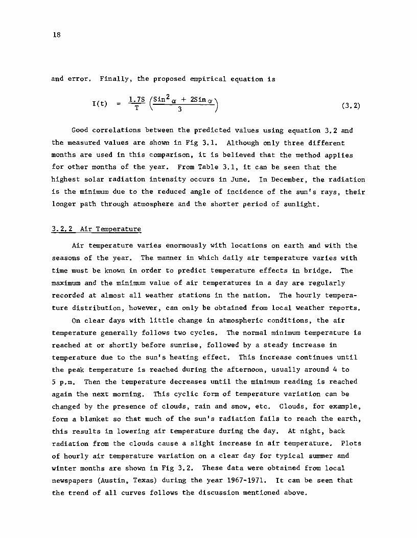
and error. Finally, the proposed empirical equation is
(3.2)
Good correlations between the predicted values using equation 3.2 and
the measured values are shown in Fig 3.1. Although only three different
months are used in this comparison, it is believed that the method applies
for other months of the year. From Table 3.1, it can be seen that the
highest solar radiation intensity occurs in June. In December, the radiation
is the minimum due to the reduced angle of i~cidence of the sun's rays, their
longer path through atmosphere and the shorter period of sunlight.
3.2.2 Air Temperature
Air temperature varies enormously with locations on earth and with the
seasons of the year. The manner in which daily air temperature varies with
time must be known in order to predict temperature effects in bridge. The
maximum and the minimum value of air temperatures in a day are regularly
recorded at almost all weather stations in the nation. The hourly tempera
ture distribution, however, can only be obtained from local weather reports.
On clear days with little change in atmospheric conditions, the air
temperature generally follows two cycles. The normal minimum temperature is
reached at or shortly before sunrise, followed by a steady increase in
temperature due to the sun's heating effect. This increase continues until
the peak temperature is reached during the afternoon, usually around 4 to
5 p.m. Then the temperature decreases until the minimum reading is reached
again the next morning. This cyclic form of temperature variation can be
changed by the presence of clouds, rain and snow, etc. Clouds, for example,
form a blanket so that much of the sun's radiation fails to reach the earth,
this results in lowering air temperature during the day. At night, back
radiation from the clouds cause a slight increase in air temperature. Plots
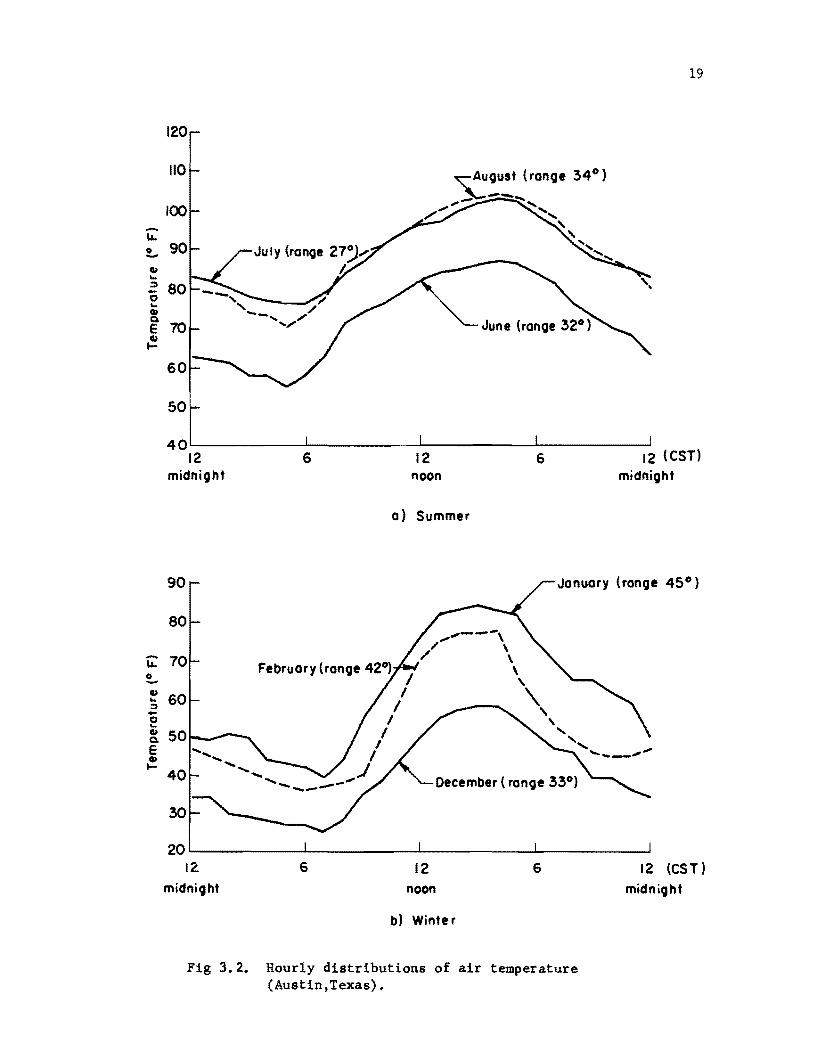
of hourly air temperature variation on a clear day for typical summer and
winter months are shown in Fig 3.2. These data were obtained from local
newspapers (Austin, Texas) during the year 1967-1971. It can be seen that
the trend of all curves follows the discussion mentioned above.
-I.L.
/00
July (range 27'", I.
19
40~----------~----------~----------~--------~ 12 6 12 6 12 (CST)
midnight noon midnight
0) Summer
90 January (range 45 0)
80
t;: 70 o -~ 60 :t -o ... ~ a. e {!!.
40
20~--------~----------~--------~----------~ 12. 6 12 6
midnight noon
b) Winte r
Fig 3.2. Hourly distributions of air temperature (Austin,Texas).
12 (CST)
midnight

20
It is worth noting that the times of high and low ambient air temperature
do not coincide with the times of maximum and minimum solar radiation inten
sity. This is true for both the daily and the yearly conditions. The month
of August is generally considered as the hottest month of the year, January
the coldest; yet the greatest intensity of radiation occurs in June and the
lowest in December. On a daily basis, the maximum air temperature normally
occurs at 4 p.m., yet the maximum solar radiation intensity occurs at noon.
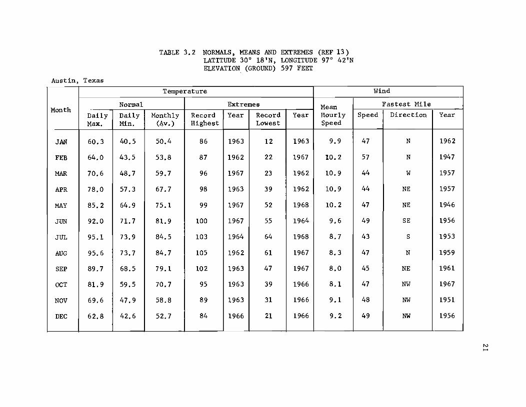
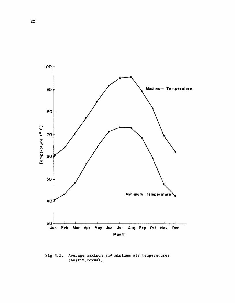
Table 3.2 summarizes temperature data as recorded in Austin, Texas. Normal
and extreme air temperature are tabulated for each month of the year. Figure
3.3 depicts the annual air temperature variation.
Studies done in this research have shown that during a period of clear
days and nights, variations of bridge temperature distribution over the con
crete cross section are small at about 2 hours after sunrise. At this time,
it is possible to assume a thermal equilibrium state in which the bridge
temperature is the same as that of surrounding air temperature. In this
study, it was also found that the range of air temperature from a minimum
value to a maximum value during a given day affects the bridge temperature
distribution. A large range of air temperature will cause a large temperature
differential over the bridge depth which in turn causes high temperature
induced stresses. Figure 3.2 depicts variations of air temperature which
yield maximum ranges of air temperature as recorded in Austin, Texas. It is
of interest to note that the range of air temperature is higher in winter
than in summer. In January, the range is 45°F while 34°F is found in August.
3.2.3 Wind Speed
Wind is known to cause an exchange of heat between surfaces of the bridge
and the environment. The speed of the wind has an effect in increasing and
lowering surface temperatures. From this research study, it is found that
maximum temperature gradients over the bridge depth are reached on a still
day. On a sunny afternoon, wind decreases temperatures on the top surface
and increases temperatures at the bottom. This effect, of course, results in
lowering the temperature gradient during the day. At night, maximum reversed
temperature gradients are also decreased by the presence of the wind.
Austin, Texas
Normal Month
Daily Daily Max. Min.
JAN 60.3 40.5
FEB 64.0 43.5
MAR 70.6 48.7
APR 78.0 57.3
MAY 85.2 64.9
JUN 92.0 71. 7
JUL 95.1 73.9
AUG 95.6 73.7
SEP 89.7 68.5
OCT 81. 9 59.5
NOV 69.6 47.9
DEC 62.8 42.6
TABLE 3.2 NORMALS, MEANS AND EXTREMES (REF 13) LATITUDE 30° 18'N, LONGITUDE 97° 42'N ELEVATION (GROUND) 597 FEET
Temperature
Extremes Mean Monthly Record Year Record Year Hourly
(4v. ) Highest Lowest Speed
50.4 86 1963 12 1963 9.9
53.8 87 1962 22 1967 10.2
59.7 96 1967 23 1962 10.9
67.7 98 1963 39 1962 10.9
75.1 99 1967 52 1968 10.2
81.9 100 1967 55 1964 9.6
84.5 103 1964 64 1968 8.7
84.7 105 1962 61 1967 8.3
79.1 102 1963 47 1967 8.0
70.7 95 1963 39 1966 8.1
58.8 89 1963 31 1966 9.1
52.7 84 1966 21 1966 9.2
Wind
Fastest Mile
Speed Direction
47 N
57 N
44 W
44 NE
47 NE
49 SE
43 S
47 N
45 NE
47 NW
48 NW
49 NW
Year
1962
1947
1957
1957
1946
1956
1953
1959
1961
1967
1951
1956
N I-'
22
u... 0 -QI ... :::J -0 ... QI Q.
E QI ....
100
90 Mallimum Temperature
80
70
60
50
Minimum Temperature
40
30~~~~--~--~--~--~--~--~~~~---L---
Jon Feb Mar Apr May Jun Jul Aug Sep Oct Nav Dec
Manth
Fig 3.3. Average maximum and minimum air temperatures (Austin, Texas) .
Wind speed is recorded by all weather stations. Table 3.2 gives the
average wind speed for each month of the year as recorded in Austin, Texas.
3.3 Heat Flow Conditions
23
The prediction of time varying bridge temperature distributions involves
the solution of the heat flow equations governing the flow of heat at the
bridge boundaries and within the bridge. In general, heat is transferred
between the bridge boundaries and the environment by radiation and convection.
Heat, on the other hand, is transferred within the bridge boundaries by con
duction. In order to estimate the temperatures in highway bridges the
relationship between atmospheric conditions and the heat transfer from the
bridge boundaries to the atmosphere must be known. The development of this
relationship will be established below.
3.3.1 Heat Flow by Radiation
Radiation is the primary mode of heat transfer which results in warming
and cooling bridge surfaces. The top surface gains heat by absorbing solar
radiation during the day and loses heat by emitting out-going radiation at
night. The amount of heat exchange between the environment and the bridge
boundaries depends on the absorptivity and emissivity of the surface, the
surface temperature, the surrounding air temperature and the presence of
clouds. Values of absorptivity of a plain concrete surface depends on its
surface color. In general, its values lie between 0.5 to 0.8. Concrete with
asphaltic surface has higher absorptivity and published values are between
0.85 to 0.98. The emissivity, on the other hand, is independent of the sur
face color. Its values lie between 0.85 to 0.95. For steel, the absorptivity
varies from 0.65 to 0.80 and the emissivity is between 0.85 to 0.95.
The heat transferred by radiation is caused by both short-wave and long
wave radiation. Heat energy absorbed by the surface from the short-wave
radiation can be estimated from
rI (3.3)

24
TABLE 3.3 VALUES OF EMISSIVITY AND ABSORPTIVITY (REF 27)
Surface
Black non-metallic surfaces such as asphalt, carbon, slate, paint, paper . . . . . . . . . . . . .
Red brick and tile, concrete and stone, rusty steel and iron, dark paints (red, brown, green, etc.) .....
Yellow and buff brick and stone, firebrick, fireclay •
White or light-cream brick, tile, paint or paper, plaster, white-wash . . . . . . . . . . . . .
Dull brass, copper, or aluminum; galvanized steel; polished iron
Emissivity 50-100 F
0.90 to 0.98
0.85 to 0.95
0.85 to 0.95
0.85 to 0.95
0.20 to 0.30
Absorptivi ty for Solar Radiation
0.85 to 0.98
0.65 to 0.80
0.50 to 0.70
0.30 to 0.50
0.40 to 0.65

where
and
Qs = heat gain by short-wave radiation,
r = absorptivity of the surface,
I = solar radiation intensity,
btu/ft 2/hr,
2 btu/ft /hr,
Values of I on a cloudless day can be obtained either by field mea
surement or by using Eq 3.2. If Eq 3.2 is used the total insolation in a
day (S) must be known.
25
The study of heat exchange which results from the long-wave radiation
follows from the Stefan-Boltzmann law. This law states that all bodies will
emit radiant electromagnetic energy at a rate which is found to be propor
tional to the fourth power of the absolute temperature of the body. The rate
at which the energy is emitted is given by
where
and
= 4 e0'9
Qe
= emitting energy,
e = emissivity,
0' = Stefan-Boltzmann constant,
9
-8 0.174 X 10 ,
= absolute temperature, oR (Rankine).
Note that OR = of + 459.67.
(3.4)
btu/ft 2/hr,
It can be shown (12) theoretically that heat loss by long-wave radiation
from bridge surfaces to the environment can be approximated by
4 4 (3.5) QL
= eO' (9 - 9:;) s
where heat loss by long-wave radiation, 2 QL = btu/ft /hr,
9s = surface temperature, oR,
9a air temperature, oR •
It has been confirmed from field measurements (51) that Eq 3.5 yields a
reasonable estimate of radiation loss between the earth's surface and the

26
environment under cloudy sky condition. Equation 3.5, however, is found to
underestimate the net heat loss from the surface when the sky is clear. This
is due to the fact that the clouds, which can be regarded as a black body,
absorbs solar radiation during the day and emits it back to the earth during
the night. According to Swinbank (43), the incoming long-wave radiation, R ,
can be estimated from
R
where R
e
and
=
=
=
=
(3.6)
incoming long-wave radiation under clear sky, btu/ft2/hr,
a co:iastant, approximately 0.496 x 10¹⁴ , btu!£t2/hr/oR6 ,
air temperature,
Equation 3.6 has been shown to represent the data from a number of sites
with a high accuracy. Therefore, net radiation loss at the top surface of a
bridge is given by
where QLC
4 6 = eO'e -eee s a
net heat loss by long-wave radiation under clear sky condition,
3.3.2 Heat Flow by Convection
(3.7)
btu/ft2/hr •
The two types of heat exchange by convection between bridge boundaries
and the environment are termed free and forced convection. In the absence of
the wind, heat is transferred from the heated surface by air motion caused by
density differences within the air. This process is known as free convection.
It is known that heat loss by forced convection is greater than by free or
natural convection.
Experiments done by Griffiths and Davis (25) show that heat loss by free
convection is proportional to the 5/4 power of the temperature difference
between two surfaces. However, it has been shown from field measurements
(51) that heat loss by convection at bridge surfaces can be approximately
27
estimated by assuming heat loss to be proportional to the first power of the
temperature difference. Such results are shown in Fig 3.4. Therefore, in
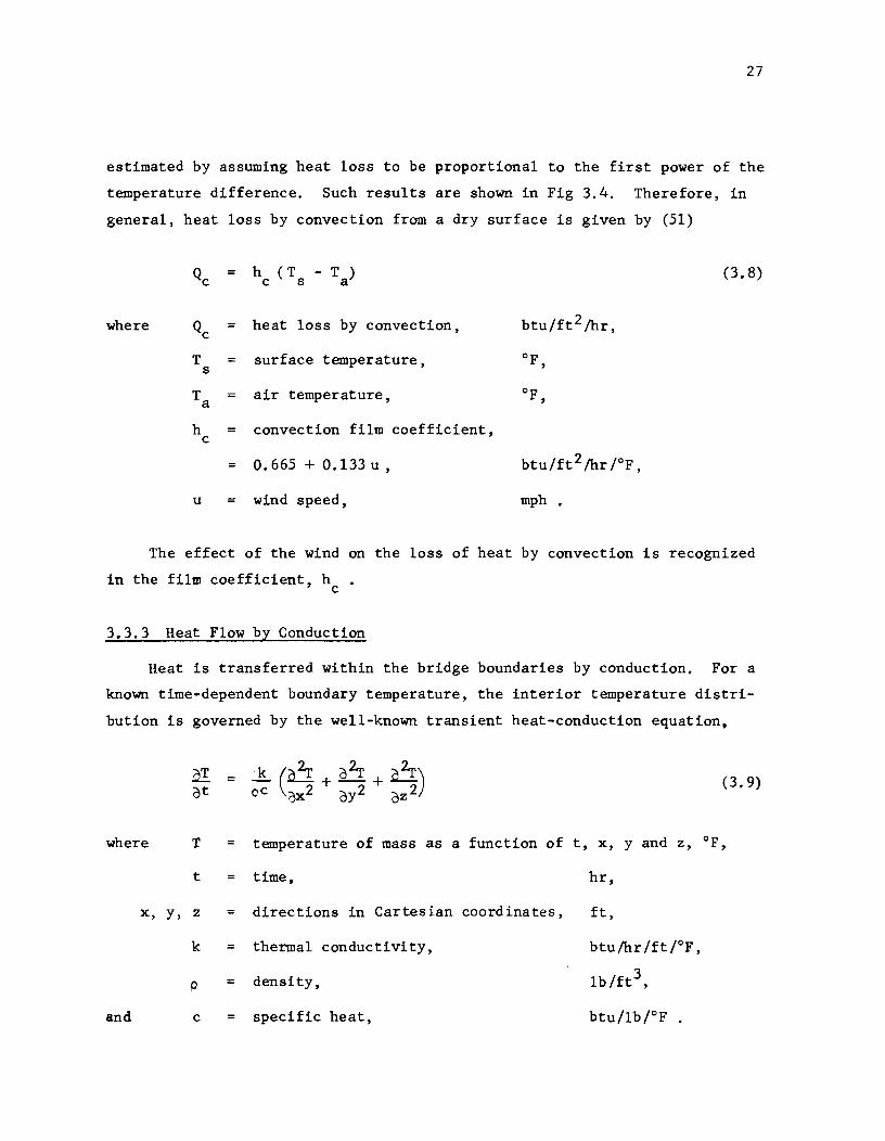
general, heat loss by convection from a dry surface is given by (51)
Qc = h (T - T ) (3.8) c s a
where Qc = heat loss by convection, btu/ft 2/hr,
T = surface temperature, of, s
T air temperature, of, a
h = convection film coefficient, c
0.665 + 0.133 u, btu/ft 2 /hr rF , u = wind speed, mph .
The effect of the wind on the loss of heat by convection is recognized
in the film coefficient, h c
3.3.3 Heat Flow by Conduction
Heat is transferred within the bridge boundaries by conduction. For a
known time-dependent boundary temperature, the interior temperature distri
bution is governed by the well-known transient heat-conduction equation,
(3.9)
where T temperature of mass as a function of t, x, y and z, OF,
t time. hr,
x, y, z = directions in Cartes ian coord ina tes, ft,
k = thermal conductivity, btu/hr/ftrF,
p = density, lb/ft3 ,
and c = specific heat, btu/lbrF
28
lI-2,4
...... ... ~
'\ c't ~o • - 2.0 ,,~'!I ...... :::J ~'\ - \'l;)'l;) ,&l
X' - 1.6 fOfO~ c: II ,,0, • u
~ --II • • 0 u 1.2 • E • i.L c: 0 0.8 • • -U II • > c: 0 u 0.4
o 2 4 6 8 10 12 14
Wind Speed (mph)
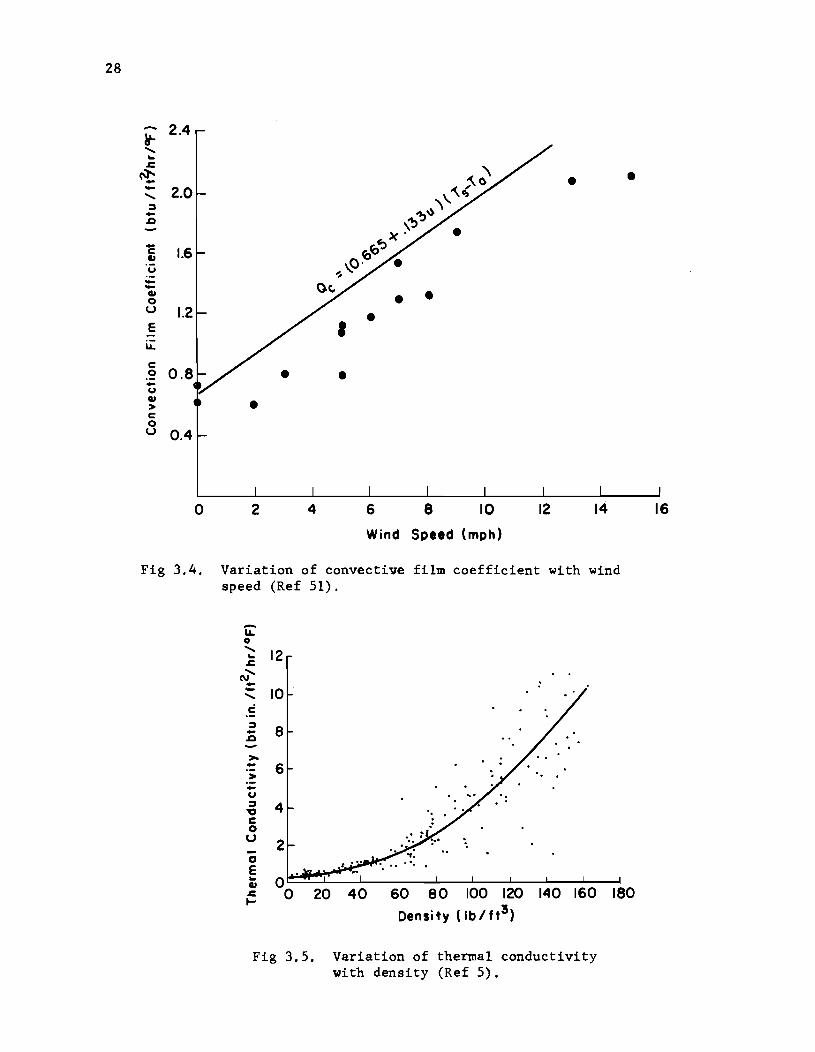
Fig 3.4. Variation of convective film coefficient with wind speed (Ref 51).
-I.L 0 ......
12 ... ~
N ...... -- 10 ...... C :::J 8 -,&l
>-- 6 > -U :::J 4 " c 0 u 2 CJ E ...
•
0 II 100 120 140 160 180 ~ 0 20 40 60 80 ....
Density (Ib/ft!)
Fig 3.5. Variation of thermal conductivity with density (Ref 5).
16
29
The thermal conductivity, k , is a specific characteristic of the
material. It indicates the capacity of a material for transferring heat.
Experiments (5) have shown that its magnitude increases as the density of
the material increases. Results of such ~xperiments are depicted in Fig 3.5.
Normally, the average thermal conductivity of concrete and steel are 0.75
and 26.6 btu/hr/ft/oF respectively. Whether the material is wet or dry
affects the thermal conductivity. It has been shown that a wet concrete has
higher thermal conductivity than a dry concrete.
Shapes of temperature distribution over the bridge depth depend mainly
on its conduction property. A steel beam, for example, because of its high
thermal conductivity, will quickly reach the temperature of the surrounding
air temperature. However, this is not true for a concrete beam. Nonlinear
temperature distribution is usually found in concrete structures as a
result of its low thermal conductivity.


CHAPTER 4. MATHEMATICAL MODELS
4.1 Introduction
The three basic mechanisms of heat transfer, conduction, convection and
radiation were discussed separately in the preceding chapter. It should be
noted, however, that the actual flow of heat is a result of all three mecha
nisms of heat transfer acting simultaneously. In general, convection
and radiation will govern the flow of heat at the boundaries while conduction
governs the heat flow within the body. Temperature induced stresses in
highway bridges can be computed only if the temperature distribution over
the cross section is known. The purpose of this chapter is, therefore, to
couple these basic mechanisms of heat transfer in an effort to arrive at a
systematic way of predicting the bridge temperature as a function of time.
Once the temperature distribution throughout the bridge cross section at any
time is known, a one-dimensional structural model is used to calculate the
temperature induced stresses. The proposed mathematical model, thus, in
cludes the heat transfer and the thermal stress analysis in one complete
system.
4.2 Bridge Temperature Prediction
The development of mathematical formulations used in predicting the
temperature distributions for both one and two-dimensional heat flow will be
discussed. Correlations of the predicted and the measured temperatures will
be presented in the next chapter.
4.2.1 One-Dimensional Model for Predicting the Temperature Distribution
The determination of time varying temperature gradients within the bridge
deck may be approximated by assuming that the heat transfers through a slab
having a finite thickness and infinite lateral dimensions. In this approach
edge effects are neglected and the heat transfer will depend on only one space
variable in the direction of the slab thickness.
31

32
For a known time-dependent boundary temperature distribution, the
interior temperatures in a homogeneous isotropic body with no internal heat
source is governed by the Fourier equation
= (4.1)
where x, y, z directions in Cartesian coordinates, ft,
t = time, hr,
T temperature at any point (x, y, z) at time t, of,
K = diffusivity,
The diffusivity, K , is a property of the material, and the time rate of
temperature change will depend on its numerical value. The diffusivity is
defined by
where
K .k
= cp
k thermal conductivity, btu/hr/ftjOF,
c specific heat, btu/lbjOF,
p density, Ib/ft 3 .
For one-dimensional heat flow, Eq 4.1 reduces to
dT dt
=
(4.2)
(4.3)
Hence, the original equation is greatly simplified as the temperature
becomes a function of t and x only. To solve Eq 4.3 it is necessary that
the initial and the boundary conditions are specified. For a bridge exposed
to atmospheric variations, the initial condition is usually referred to as the
time at which the temperature distribution throughout the bridge is uniform.

33
The boundary conditions are the known surface temperatures. These tempera
tures can be predicted by considering the heat exchange process which takes
place at bridge surfaces. Heat is transferred from the environment to bridge
surfaces by convection and radiation.
At the top surface, heat balance can be expressed as
Heat absorbed from short wave radiation
Heat lost by convection + Heat lost by long wave radiation + Heat lost by conduction.
Under clear sky condition, the above equation is then represented by a sum of
EQS 3.8, 3.7, and Eq 4.3 at initial conditions:
where
rI h (T - T ) + (e (j e 4 - e € e 6) c s a s a k(~) OX x=O
r absorptivity of the surface,
e = emissivity of the surface,
I total incoming solar radiation intensity,
h c = convection film coefficient of the top surface,
k thermal conductivity of the material,
T top surface temperature, s
T = top air temperature, a
8s
top surface temperature, oR,
== top air temperature, oR,
(4.4)
Stefan-Boltzmann constant, == 0.174 X 10⁻⁸
btu/ft2
/hr/OR4
€ coefficient of incoming long wave radiation, and
= temperature gradient in the x-direction
At the bottom surface,the heat balance equation is
Heat gained by conduction Heat lost by convection + Heat lost by long wave radiation.
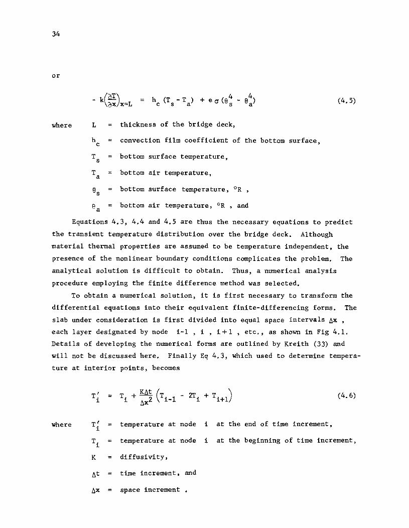
34
or
k(a±.) oX x=L (4.5)
where L = thickness of the bridge deck,
h = c convection film coefficient of the bottom surface,
T = bottom surface temperature, s
T = bottom air temperature, a
Ss = bottom surface temperature, oR ,
8a = bottom air temperature, QR , and
Equations 4.3, 4.4 and 4.5 are thus the necessary equations to predict
the transient temperature distribution over the bridge deck. Although
material thermal properties are assumed to be temperature independent, the
presence of the nonlinear boundary conditions complicates the problem. The
analytical solution is difficult to obtain. Thus, a numerical analysis
procedure employing the finite difference method was selected.
To obtain a numerical solution, it is first necessary to transform the
differential equations into their equivalent finite-differencing forms. The
slab under consideration is first divided into equal space intervals ~x ,
each layer designated by node i-l, i , i + 1 , etc., as shown in Fig 4.l.
Details of developing the numerical forms are outlined by Kreith (33) and
will not be discussed here. Finally Eq 4.3, which used to determine tempera
ture at interior points, becomes
T~ K~t ( zr i + Ti +l ) (4.6) = Ti + --Z Ti _1 -l. ~x
where T~ = temperature at node i at the end of time increment, l.
Ti = temperature at node i at the beginning of time increment,
K = diffusivity,
~t time increment, and
~x = space increment

Top Surface
.2
i-J • 6f ei
6X Thickness e i+1
e etc.
Bottom Surface
Fig 4.1. A typical slab cross section showing nodal point numbering.
35

36
Equation 4.6 allows one to compute the temperature at the interior
points at the end of each time increment if temperature distribution at the
beginning of the time increment is known. The surface temperature is com
puted by using Eqs 4.4 and 4.5. At the top surface, the differencing scheme
is
rI
where i=l. Hence, Ti
_1
no longer exists, Substituting Ti
_1 from
Eq 4.6 into Eq 4.7 yields
where
T' 1
0:'1
a1
1'1
=
=
=
- 2 - 2 ~xhc
k
~xhc 2 -k-' and
2~ 4 6 (rI - eO' 81 + e € 8a) k
Similarly, at the bottom surface, Eq 4.5 is rewritten as
4 = h (T - T ) + e 0' (8 c nan
By substituting for Tn+1 from Eq 4.6 into Eq 4.9, yields
(4.7)
(4.8)
(4.9)
(4.10)
where - 2 - 2 l\xhc
0:'2 = k
l\xhc a2 = 2--
k
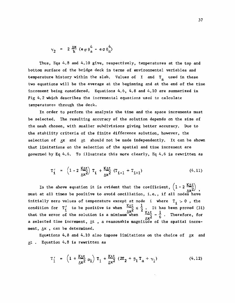
37
= 2 1e. (e a e 4 - e a e 4) k a n
Thus, Eqs 4.8 and 4.10 give, respectively, temperatures at the top and
bottom surface of the bridge deck in terms of environmental variables and
temperature history within the slab. Values of I and T a used in these
two equations will be the average at the beginning and at the end of the time
increment being considered. Equations 4.6, 4.8 and 4.10 are summarized in
Fig 4.2 which describes the incremental equations used to calculate
temperatures through the deck.
In order to perform the analysis the time and the space increments must
be selected. The resulting accuracy of the solution depends on the size of
the mesh chosen, with smaller subdivisions giving better accuracy. Due to
the stability criteria of the finite difference solution, however, the
selection of 6x and 6t should not be made independently. It can be shown
that limitations on the selection of the spatial and time increment are
governed by Eq 4.6. To illustrate this more clearly, Eq 4.6 is rewritten as
T' i
(4.11)
In the above equation it is evident that the coefficient, (1 - 2 KA~) 6x ,
must at all times be positive to avoid oscillation, i.e., if all nodes have
initially zero values of temperature except at node i where T. > 0 , the KAt 1
l.
condition for T' to be positive is when s; - It has been proved (31) i 6x2 2 K t 1 that the error of the solution is a minimum when ~ 6 . Therefore, for 6x
a selected time increment, 6t , a reasonable magnitude of the spatial incre-
ment, 6x , can be determined.
Equations 4.8 and 4.10 also impose limitations on the choice of 6x and
6t. Equation 4.8 is rewritten as
T' 1
= ( 1 + KAt) T + KA t (zr 2 + Q 1 Ta + Yl
) 6x2 0'1 1 6x2 f.'
(4.12)

38
I Top T' :: TI + ~~~ (aIT, + 2Tt + ~I To + )", ) 777 7 • 1117777 I
.2 T' :: K6t z Tz + 6X 2 tTl - 2Tt + T3 )
t:..X
r' K6t • 3
:: 1; + ~ (Tt - 2T3 + T4 ) :5 6X t:..X
-4 etc.
etc .
• n-I
1111,11111/ n Bottom
Fig 4.2. A typical slab cross section shOWing equations used in calculating temperatures.
(4.8 )
(4.6 )

Therefore, in accordance with the previous discussion the following
condition must be satisfied
39
(4.13)
Since the above equation involves the varying values of h ,the inc
equality must be checked at each time interval to ensure the numerical
stability.
In summary, the method discussed above involves the following steps:
at the initial time;
1. Obtain material thermal properties; conductivity, specific heat, etc.,
2. Establish time and space increment, ~t and ~x respectively,
3. Establish initial temperature distribution over the depth of the slab,
and for each time increment, ~t ;
4. Input environmental variables; air temperature, insolation intensity and wind speed,
5. Compute top and bottom surface temperature,
6. Compute all interior nodal temperatures, and
7. Repeat for the next time increment.
4.2.2 Two-Dimensional Model for Predicting the Temperature Distribution
In the preceding section, the temperature and the heat flow in one
spatial dimension and the method of analysis were discussed. When the bridge
has an irregular shape of cross section, the one-dimensional treatment may no
longer be satisfactory. For example, studies have shown, in Chapter 5, that
the temperature distribution over the cross section of a pan-type bridge is
nonlinear in both the vertical and transverse direction. Good correlations
between the measured and predicted temperature distributions are obtained
when heat is considered to flow two dimensionally. Also, in Chapter 7,
40
studies of temperature effects in a composite precast pretensioned bridge
show that although most of the slab portions experience one-dimensional heat
flow from the top to the bottom, the flow of heat in the I-beam is in two
dimensions. Moreover, the orientation of the bridge which is not in the
east-west direction also necessitates the development of a two-dimensional
heat flow model, which enables one to take into account the side heating
effects.
In this section, a method of predicting the temperature distribution in
a bridge which has constant temperature variations along its length but which
may have arbitrary temperature distribution in the cross-sectional plane will
be presented. Again, the classical approach to the exact solution will not
be considered due to the difficulties in treating the geometry and the
boundary conditions. Although there are several approximate methods avail
able for the solution to this type of problem, the finite element method was
selected for this work. The advantages of the finite element method are that
complex bodies composed of different materials are easily represented. In
addition, the method allows temperature or heat flow boundary conditions to
be specified at any nodal point in the body. It can also be shown mathe
matically, that the method converges to the exact solution as the number of
elements is increased.
In the finite element method it is necessary to find a functional such
that the minimization of this functional will give functions which satisfy
the field equations and boundary conditions of the problem of interest. Many
functionals have been used by many researchers in solving the uncoupled field
problem. Wilson and Nickell (53) used a functional proposed by Gurtin (26)
to solve transient heat flow problems. A residual approach based on
Galerkin's principle was used by Zienkiewicz and Parekh (56). Another func
tional was also presented by Brisbane, Becker and Parr (9) for thermoelastic
stress analysis. It should be pointed out that whichever functional is used,
the final forms for the finite element equations will essentially be the same.
Instead of following the formal mathematical method, Wilson (52) used another
approach. He showed that a physical interpretation of the heat transfer
process in a solid body could also be used to formulate equilibrium equations
needed in the finite element method.

41
Since the functional given in Ref 9 is relatively easy to handle, it
will be used in formulating the mathematical model to predict bridge tempera
tures. The functional, with no internal heat source, is defined as
TT (U, U) = J {~'Z U • ~ y U + P c U ir 1 d v - J ~ . ~ U d s (4.14) v s
where v = volume of the domain,
s = surface of the domain1s boundary,
k k(xi ) = conductivity tensor for an anisotropic material, ~ ~
c = c(xi) specific heat,
p = p (xi) = density,
~ = q(xi) heat flux vector across a boundary, ,....,
i unit normal vector, n n(x )
U U(xi,t) = temperature,
. U(xi,t) U time derivative of temperature,
~ U = gradient of U, and ,....,
xi coordinates.
If temperature U is assumed to take a certain variation over the
element and that it can be defined by the nodal point temperature, u , the
functional above· becomes TT(U, u). The equilibrium and the boundary
equations can then be obtained by the virtue of the principle of minimum
potential energy, i.e., by
aJ:!. ( • ) u , u o u ,...., ,...., 0 (4.15)
Let U Nu (4.16)
. Nu then U
and ~ U = ~Nu Du (4.18) ,....,,....,,...., ~,....,

42
Substituting above values into Eq 4.14, the result in the matrix form is
rr(u , ~) (4.19)
Applying Eq 4.15 to the above equation, then
I{ T T·~ ITT g, ~g~ + pc;: ~ u r d v - ~ ~ ;! d s v s
= 0 (4.20)
In applying Eq 4.20 to highway bridge structures the heat flux q will '"
be the combination of a convective heat flux, ~ , over Sl and a radiation
heat flux, ~r ' over S2' These vectors are expressed, from Chapter 3, as
= h (U - U ) c a (4.21)
under clear sky
(4.22)
The convective vector, Q , can be treated exactly in the finite element ""c
formulation. However, this is not the case for the radiation term because
SLC contains the nonlinear temperature field. According to Eq 3.7
eo-(U + 460)4 - 0.496 X 10⁻¹⁴ (Ua + 460)6 e (4.23)
To simplify the problem, the temperature of the previous time is used
for U in Eq 4.23. In doing this, the time increment must be kept small to
minimize the error. In fact, in the finite difference formulation discussed
in section 4.2.1, previous values of temperature were used explicitly with
out considering this as the source of error.
Equation 4.20 can then be rewritten as
,(4.24)

43
. (B + H) u q* + h* or ·C u +
~~ ~ ~,....." (4.25)
where C = pC I NTN d v ~ ''/v'"'''' ,.....,
(4.26)
B = I ~T1s ;g d v ~ t.. v """'''''''' ,.....,
(4.27)
H h I NTN ds ~ c IJ ~ ~
sl (4.28)
q* = J NTnT Q ds ,.....,,....., ,.....,r s2
(4.29)
and h* = h U I NT ds c a J ~
(4.30) s1
Coefficients for the matrices and vectors from Eqs 4.26 through 4.30
can be computed if the shape of the element and the form of temperature
distribution over the element are specified. The triangular element with
linear temperature field over the element is used here, see Fig 4.3.
Matrices of the above equations are given explicitly in Appendix A. For a
quadrilateral element, coefficients are formed from four triangular elements
as shown in Fig 4.4. The unknown temperature at node 5 is eliminated from
the equations by the method of static condensation.
Coefficients of the matrix C given in Appendix A follow from the
assumption that the heat capacity is lumped at the nodal points. This
lumped method results in a diagonal heat capacity matrix, thus requiring less
computation effort. The loss of accuracy of the solution due to this approxi
mation, however, has been shown to be small (53).
For convenience, Eq 4.25 will be rewritten as
. £ ~t + ~ ~t = F (4.31)
where K = B + H (4.32) ~ ~ ~
and F = q* + h* (4.33) ~ ~

44
y
"""""----......
j I U j
bj
~--------------------------------~-x
Fig 4.3. A typical triangular element.
y
J.i1--------- 2
~-------------------------~x
Fig 4.4. A typical quadrilateral element.

45
If the temperature at each node is assumed to vary linearly within the
time increment, the rate of change in temperature is then constant and is
given by
= (4.34)
where time increment
Substituting Eq 4.34 into Eq 4.31 and regrouping terms, yield
K* u ~ ,....",t F* (4.35)
where K* (4.36)
and F* (4.37)
Equation 4.35 is now a system of linear equations and can be solved for
the new temperature. If time increment and wind speed are constant for all
time steps, the K* will then be independent of the time variable. In such
a case, K* needs to be triangularized only once resulting in computational
efficiency for the subsequent time increments.
In summary, the method involves the following steps of calculation. At
the initial time,
1. Calculate C and K , ~ ~
2. Modify for temperature boundary conditions,
3. Form K* , ~
4. Triangularize K* ~
,
and for each time increment, tlt ,
5. Calculate F
where gs is the average value at time t and (t-tlt) ,

46
Q is the value at time (t-6t) , '" LC .
h* is the average value at time t and (t-6t) ,
.6. Calculate F* '"
7. Solve equation F* , and '"
8. Repeat for next time increment.
4.3 Thermal Stress Analysis
After temperature throughout the bridge structure is known, temperature
stresses can then be computed. These stresses, however, are only approximate
because of the difficulty in determining the elastic modulus of concrete and
its coefficient of thermal expansion. Besides, the unknown degree of edge
restraints and the unexpected unsymmetrical geometry of the bridge also affect
the resultant stress. The theory.of the stress analysis, therefore, inevit
ably involves certain idealizations of the structure and material properties.
In this work, temperature induced stresses are computed based on one-dimen
sional elastic beam theory and includes the following assumptions:
1. Temperature variation is constant along the length of the bridge but can vary in any manner over the cross section of the bridge,
2. Thermal strains vary linearly with temperature changes,
3. The principle of superposition is valid,
4. An isoptropic material,
5. Material properties are temperature independent, and
6. Plane sections remain plane after deformation.
In addition, the upcoming discussion will follow the classical thermo
elasticity theory as developed by Duhamel and Neumann. This theory assumes
that, although the state of strain of an elastic solid is affected by a
nonuniform temperature distribution, the heat conduction process is unaffected
by a deformation (7). This assumption is, of course, an approximation in
the transient thermal problem. In order to understand the effects of tempera
ture, a typical beam section away from the ends is represented by a set of
47
springs and straight rods as depicted in Fig 4.5a. Each spring has a spring
constant E, i.e., the modulus of elasticity of the material. Originally,
at zero reference temperature, all springs have the same length and are free
from stress. If each spring is then subjected to the temperature rise as
shown in Fig 4.5b, all springs will expand unequally and the system will seek
a new equilibrium configuration. By removing the right connecting rod, each
spring will expand freely and with zero stress. According to the second
assumption mentioned above, thermal strain in each spring is
where
e! ~
=
Q' T. ~
i = 1,5
th thermal strain in the i spring,
Q' coefficient of thermal expansion, and
= temperature rise in the ith spring.
(4.38)
The position of the system at this stage is shown in Fig 4.5c which
violates the assumption that the plane section remains plane after defor
mation. To restore the original position, an appropriate compressive force
is applied to each spring, thus resulting the compressive stress of
where
- E Q'T i i 1,5
= thermal stress in the ith spring, and
E = spring constant.
(4.39)
For sections throughout the beam to maintain the same condition, it is
necessary to distribute the compressive force of the magnitude (Eq 4.39) at
the ends of the beam only. However, if the beam is free from external forces,
the longitudinal stress must vanish on the ends. To eliminate the end forces,
tensile stress of the magnitude E Q' T i is applied to each spring at the ends
of the beam. According to Saint Venant's principle, stresses and deformations
at sections away from the ends can be estimated by the use of statically
equivalent forces. Under these forces, the resulting strain distribution
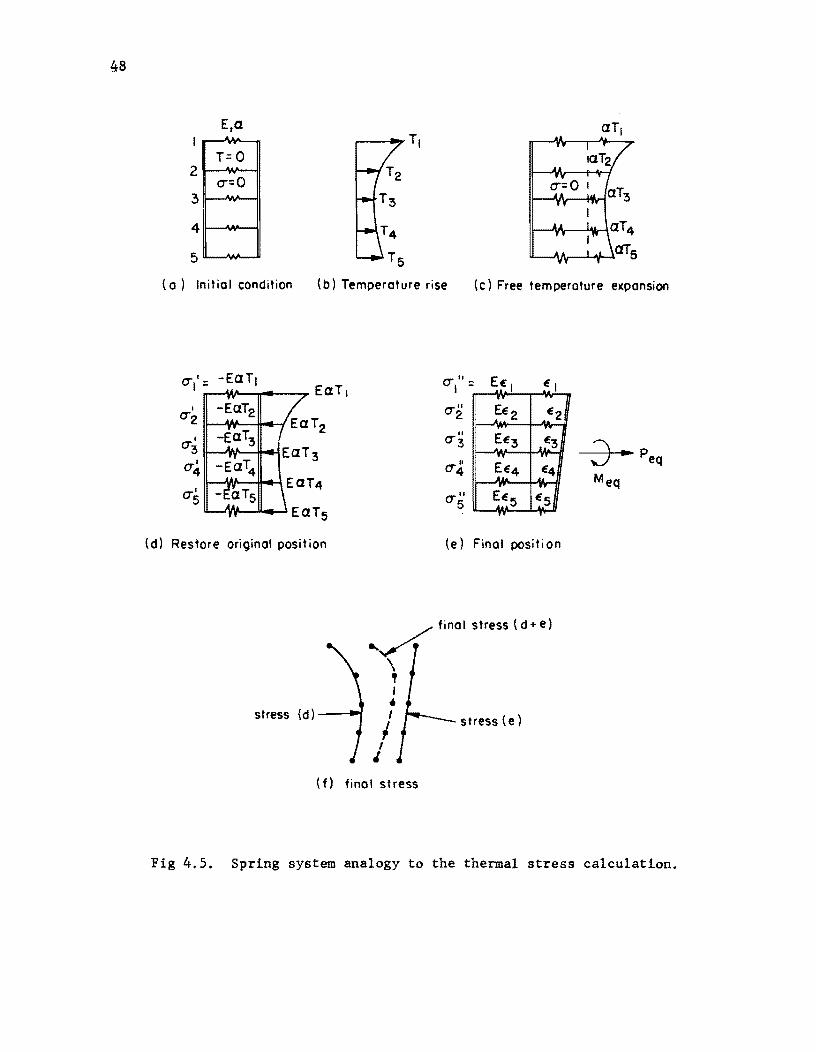
48
2 T=O
C'J"=O 311---NlJ~
4 II---W---li
5 II..-."""",~
(a) Initial condition (b) Temperature rise (c) Free temperature expansion
,.,. " -vI -
0-" 2
(d) Restore original position (e) Final position
.... /, final stress (d+e)
stress (d) ---1111
\ , I
j
I
I I
J
(f) final stress
stress(e)
---3---- P eq
Meq
Fig 4.5. Spring system analogy to the thermal stress calculation.

49
will be linear over the depth and the final position of the spring system
satisfies the assumption of plane sections remaining plane after deformation,
Fig 4.Se. Stress in each spring is
" E " i = 1,S (4.40) O'i € i
where " = stress in the ith spring due to the statically equivalent O'i forces,
and " th
due to the statically equivalent €i = strain in the i spring forces.
Temperature induced stress in each spring is thus obtained by super
imposing stresses of Fig 4.Sd and Fig 4.Se. Final stress in each spring is,
Fig 4.Sf,
i 1,S (4.41)
where = thermal induces stress in the ith spring.
It should be pointed out that the application of Eq 4.41 is valid for
sections at some distance from the ends of the beam. At the ends of the
beam the resultant stresses must approach zero. Also, the deformed shape
resulting from the temperature differential can be obtained by considering
the system subjected to statically equivalent forces applied at both ends.
4.3.1 Thermal Stress Analysis using the One-Dimensional Temperature Distribution Model
The prediction of temperature distribution using this mathematical model
was discussed in section 4.2.1. In calculating thermally induced stresses,
consider a unit width of slab cross section subjected to temperature distri
bution as shown in Fig 4.6. The equivalent force and moment about the
neutral axis x are
p eq J
d/2 E ct T(y) dy
- d/2 (4.42)

50
- ,-----
d,t. 2
-'-
y
+ I
h
h
N.A.
f~1 _-__ -t-
f ... PI
T (y)
x
n-I n -..,--------t~ .. Poi f n is even
EdTn
Fig 4.6. Gne-dimensional model showing the method of calculating. ~tempera~urel .forces.
y k ~ __ ~Tk
Ye I 1--_1-1 ..
r-t--;::::l-- Ea Td A
---+-+ X (b) Quadrilateral element
.-_ .. Tj
(a) cross secti on k
( c) Tr i angular element
Fig 4.1. Two-dimens~on~l model showing Ithe ~thod of calcula:tihg t·emperature forces.

and d/2 J E Q' T (y) Y dy
- d/2
51
(4.43)
The close form of integral calculus cannot be used directly since the
shape of the temperature distribution is not available. As temperatures are
predicted only at nodal points, the numerical integration procedure employing
Simpson's and trapezoidal rule are used. By fitting a parabola through
three successive points, the force and the location of the centroid under
this parabolic temperature distribution are
(4.44)
and (4.45)
On the other hand, if the temperature is assumed to be linear over two
successive points, the following is obtained
p o
h(2T + T 1) n n-
Finally, Eqs 4.42 and 4.43 are written numerically as
if n is odd
p eq
(n-1) /2 L: P. i=l 1
(4.46)
(4.47)
(4.48)
(4.49)

52
if n is even
p eq
(n-2) /2 L: i=l
P. + p ~ 0
(4.50)
and (n-2)/2 [d {- 'l {d - ~ L: P. -2 - Yi + (i -1) 2h r - P -2 - (h - Y ) r (4. 51) i=l ~ , ~ 0 0 )
Temperature induced stress at a point having distance y from the
neutral axis is, therefore,
=
4.3.2 Thermal Stress Analysis using the Two-Dimensional Temperature Distribution Model
(4.52)
The prediction of temperature distribution using this mathematical model
was discussed in section 4.2.2. In determining temperature induced stresses,
equivalent end force and moments are computed numerically. For a linear
temperature distribution over the element, Fig 4.7, the equivalent end force
of element e is
P e = A E T e e Q'e av (4.53)
where T av 1 "4 (T i + T j + T k + T t) for a quadrilateral
and
A e thermal
T av
E e and
expansion
distance from the
for a triangle.
Q'e are the area, modulus of elasticity and coefficient of
of element e respectively. If Ye and x denote the e
location of force P to the principal x-axis and y-axis e respectively. the equivalent end moments of element e are given by
~ = e P x e e
(4.54)

If the bridge section is divided into n number of elements, the
total equivalent force and moments will be, respectively,
P eq n
l: e=l
P e
~ eq n
l: e=l
P x e e
53
(4.55)
Finally, temperature induced stress at point i having coordinate
(xi'Yi) is
Peq Yi x xi -+-M +-MY -E 1'\1 T
A I I i "'"i i x eq y eq
4.3.3 Applications of the Method to Different Types of Bridge Geometry
(4.56)
It is important to note that the foregoing discussion is applicable only
when the structural deformations, flexural and axial displacements, caused by
equivalent forces are permitted to take place freely. When the boundary
conditions are such that these deformations are prevented, additional stresses
associated with the restraining forces must be considered.
A simply supported bridge is shown in Fig 4.8a. The thermal stress
distribution at a section which is far away from the ends, under free movement
condition, can be obtained directly by using Eq 4.41. However, if the bridge
is supported on friction bearings, free movement is now prevented and friction
forces are developed. Stresses caused by these friction forces must then be
superimposed to the above stresses to yield the final stresses. Similarly,
in the case of a continuous bridge, Fig 4.8b, the free vertical displacement
is not allowed. Thermal induced stresses at section 1-1, however, can be
M in Eq 4.52. Another example is eq calculated by substituting for
when the bridge has varying thicknesses along the length, Fig 4.8c. In this
case, the bridge is first divided into a number of prismatic beam members.
It can be seen that the method approximates the geometry of the bridge in the
region of the varying thickness. For each beam element the equivalent forces
are computed. At nodal points where adjacent elements have different
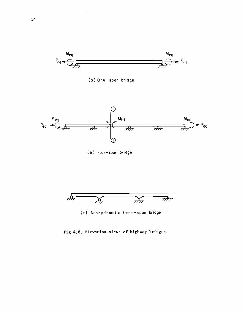
54
M~ M~
Peq~~k----------~......,L 0 .. Peq
(a) One-span bridge
CD
Meq I MH Meq
Peq ~ G ;J.r;;~====:::::::;;J37;:::==)~'1It:C===;;;;;;::::::====::;¥T:::::::=======l7b~ Peq
CD
(b) Four-span brid(;Je
(c) Non- prismatic three - span bridge
Fig 4.8. Elevation views of highway bridges.

55
thicknesses, there will be unbalanced forces and moments. Stresses caused by
equivalent forces can then be obtained by using the stiffness method. Final
stresses are then computed using Eq 4.41.

CHAPTER 5. VERIFICATIONS OF THE MATHEMATICAL MODELS
5.1 Introduction
The purpose of this chapter is to correlate existing measured bridge
temperature distributions with the results computed from theoretical con
siderations developed in Chapter 4. Both one- and two-dimensional heat
transfer models will be verified to validate the method used. Although the
analyses involved approximations of the bridge cross-section, and the lack of
actual information on the material properties, the agreement in the gross
trends and the orders of magnitude is considered to be satisfactory. Two
types of highway bridge as shown in Fig 5.1 and Fig 5.4 were used for this
purpose.
5.2 Temperature Prediction by the One-Dimensional Model
The selected bridge was a three-span concrete slab structure located in
Houston, Texas. The slab thickness varies from 17 inches to a maximum of
34 inches at the central support. Partial plan and elevation views of the
bridge are shown in Fig 5.1. A field test was performed on 24 August 1974.
The solar radiation intensity, ambient air temperature and wind speed were
recorded. Surface temperatures were also measured at selected points. The
locations of the points are depicted in Fig 5.1. Details of the field test
can be found in Ref 49.
The test day was considered to be partly clear and partly cloudy. As
is shown in Fig 5.2, the variation of the measured solar radiation intensity
experienced a great deal of fluctuations. Although the maximum value is
approximately 90 percent of the maximum intensity recorded on a clear day,
the daily total radiation is only about 50 percent of that for a clear day.
The distribution of the measured air temperature is also shown in Fig 5.2.
The range of the temperature from the minimum to the maximum value was
observed to be only 10°F. The field test was terminated at approximately
4:30 p.m. due to a heavy rain.
57
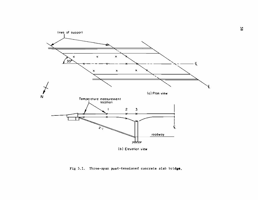
lines of support
)( x
"~ "" ....... )(-- ........ -
"'-X X
... ... , .......
.....
I .......... ..........
(a) Plan view N
Tempe,rature measurement location
2 3 I
~ I ~ I
I i
roadway
(b) Elevation view
Fig 5.1. Three-span post-tensioned concrete slab brida_.
i
'i
V1 co
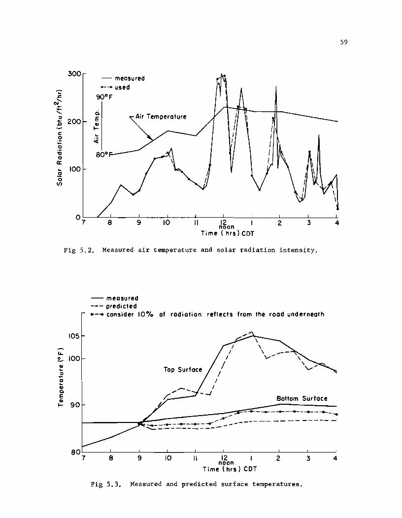
300 - measured
..... - used -... gooF s:. N ...... --...... 0. Air Temperature ::I
200 E -,Q cu ~
c: ... 0 .-- <[ 0
'0 0 0:: ... 100 ~ 0
(/)
8 9 10 II 12 noon 2 3 4
Time ( hrs) COT
Fig 5.2. Measured air temperature and solar radiation intensity.
1.1.. 0 -cu ... ::I -0 ... cu 0. E cu ~
105
100
90
-- measured --- predi cted .. - .. consider 10 % of radiation reflects from the road underneath
Top Surface
I --1
/ /
I
I I
I
Bottom Surface
L-~~===:-.... -:::::--="": --- -- -- -- ----- ---..-- ........ -~--+--........ ----'-------------
80~----~----~----~----~--~~--~----~----~----~ 7 8 9 10 II 12 2 3 4
noon Time (hrs) COT
Fig 5.3. Measured and predicted surface temperatures.
59
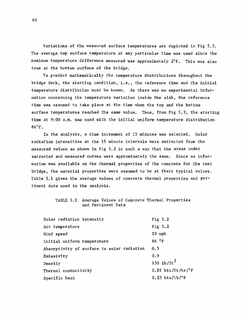
60
Variations of the measured surface temperatures are depicted in Fig 5.3.
The average top surface temperature at any particular time was used since the
maximum temperature difference measured was approximately 2°F. This was also
true at the bottom surface of the bridge.
To predict mathematically the temperature distributions throughout the
bridge deck, the starting condition, i.e., the reference time and the initial
temperature distribution must be known. As there was no experimental infor
mation concerning the temperature variation inside the slab, the reference
time was assumed to take place at the time when the top and the bottom
surface temperatures reached the same value. Thus, from Fig 5.3, the starting
time at 9:00 a.m. was used with the initial uniform temperature distribution
86°F.
In the analysis, a time increment of 15 minutes was selected. Solar
radiation intensities at the 15 minute intervals were extracted from the
measured values as shown in Fig 5.2 in such a way that the areas under
extracted and measured curves were approximately the same. Since no infor
mation was available on the thermal properties of the concrete for the test
bridge, the material properties were assumed to be at their typical values.
Table 5.1 gives the average values of concrete thermal properties and per
tinent data used in the analysis.
TABLE 5.1 Average Values of Concrete Thermal Properties and Pertinent Data
Solar radiation intensity
Air temperature
Wind speed
Initial uniform temperature
Absorptivity of surface to solar radiation
Emissivity
Density
Thermal conductivity
Specific heat
Fig 5.2
Fig 5.2
10 mph
86 of
0.5
0.9
150 lb/ft3
0.81 btu/ft/hr/oF
0.23 btu/lb/oF

61
Three different slab thicknesses, i.e., 17 inches, 25.5 inches and
34 inches at sections 1, 2 and 3 respectively, Fig 5.lb. were considered
in the analysis. In each case, however, the temperatures computed at the
surfaces were identical. The predicted top and bottom surface temperatures
are shown in Fig 5.3. The comparison between measured and predicted top
surface temperatures was found to be satisfactory. However, there was a
greater discrepancy at the bottom surface of the bridge which has been
attributed to the fact that the sun's rays reflected from the roadway under
neath were neglected in the analysis. Since the orientation of the bridge
is not in the east-west direction, the bottom surface receives a portion of
the solar radiation intensity thus influencing its temperature. Subsequently
an additional analysis was made by assuming that the bottom surface absorbed
10 percent of the measured solar radiation intensity. The results of this
analysis are also shown in Fig 5.3. It should be noted that the above
assumption, which is felt to be reasonable, results in a better agreement
with the measured temperatures.
The above comparison of measured and predicted temperature variations,
although limited to the surfaces of the bridge, provide positive evidence
that actual bridge temperature distributions over the depth under daily
environmental changes can be predicted in a satisfactory way. In the next
example, where more extensive data from field measurements were available,
comparisons of temperature distributions throughout the depth during a summer
day and a winter night will be given. Comparison of vertical thermal
deflections during the summer day will also be illustrated.
5.3 Temperature Prediction by the Two-Dimensional Model
The selected bridge was a simply supported structure with a span of
46 feet. Its cross-section consisted of 14 pan-type reinforced concrete
beams. A partial cross-section including the edge beam and typical interior
beams of the bridge is shown in Fig 5.4. The bridge is located in San
Antonio, Texas.
The bridge was field tested under temperature effects by Wah and Kirksey
(48). A total of 390 thermocouples was instrumented in the bridge to record
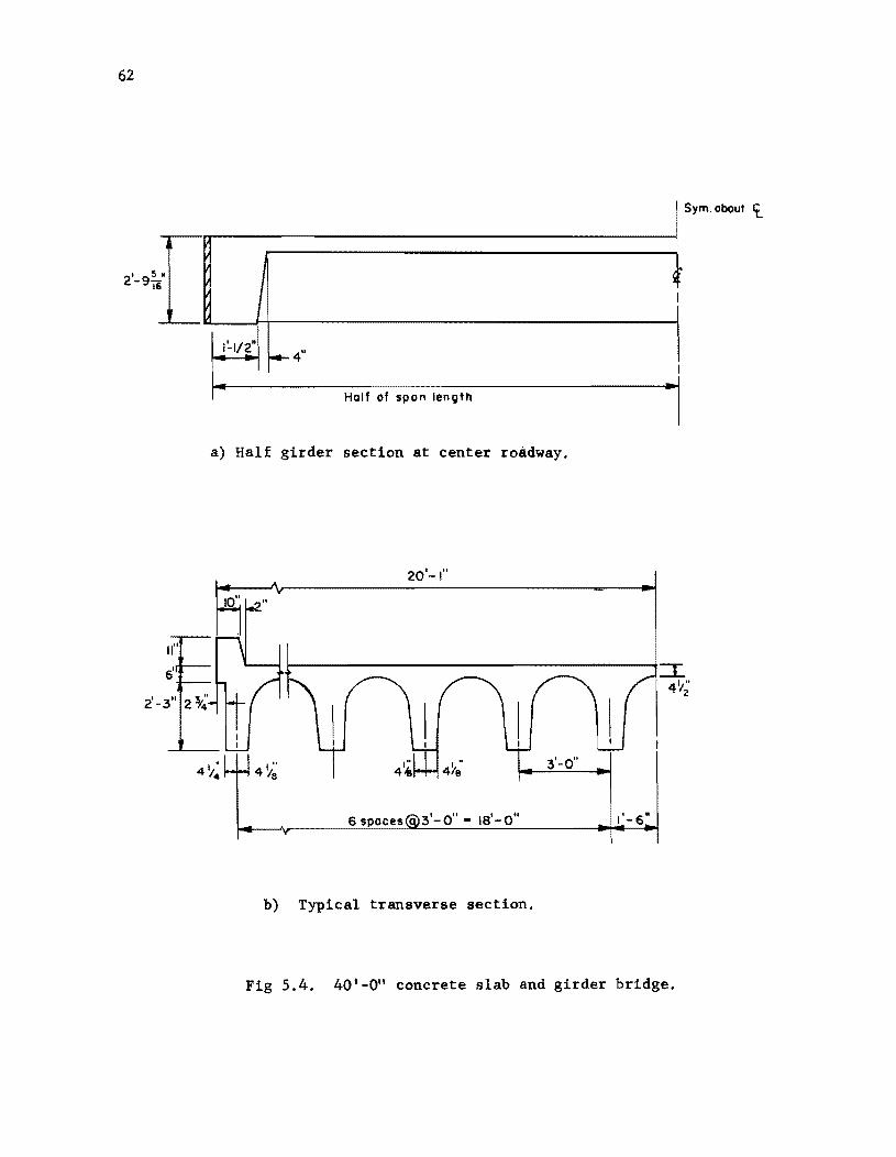
62
2'-9~[ 16
II"
6'
2'-3" 2:;-~'
Sym. about <t
l' j
1~1/2· r--- 4" I
Half of span lenQth
a) Half girder section at center roadway.
20'-1"
~I 1 ..
4 /z
3'-0"
6 spaces 3'-0" - 18'-0" 1'-6"
b) Typical transverse section.
Fig 5.4. 40'-0" concrete slab and girder bridge.
63
temperature. Thirteen thermocouples, six in the slab portion and the
remaining seven in the beam portion, were used to measure temperatures over
the depth. The location of thermocouples in one typical beam is shown in
Fig 5.5a. Tests were made on August 8 and 9, 1967 and on December 11, 1967.
Surrounding air temperatures, sky condition and concrete temperatures were
recorded at 1-1/2 hour intervals. Details of these field measurements are
described in Ref 48.
The finite element mesh of a typical beam section is depicted in Fig
5.5b. Three element layers were used over the slab thickness while two
layers were used across the half-width of the beam. Triangular as well as
quadrilateral elements were used in this idealization.
5.3.1 Temperature Prediction on August 8, 1967
August is usually considered as the hottest summer month. On August 8,
1967, a field test was performed from 6:00 a.m. to 8:00 p.m. (48). Table
5.2 gives the ambient air temperatures and a brief description of weather
conditions during the test period. The solar radiation intensity received on
a horizontal surface, on the other hand, was obtained from the U.S. Weather
Bureau Reports (14).
From the study of temperature logs given in Ref 48, it was apparent that
the bridge temperature distribution was almost uniform at 9:30 a.m. Hence,
for simplicity of input data, it was assumed that the starting time is at
9:30 a.m. and the temperature is uniform over the cross section at 89°F,
Fig 5.6a. Wind speed, recorded as light wind, was assumed to be constant
at 10 mph for every time increment. This amount of wind speed is usually
considered as the average value for a normal day. Air temperatures used in
the analysis were the average values of the measured top and bottom ambient
temperatures given in Table 5.2. Two values of daily total insolation inten
sity, i.e., 100 and 80 percent of the value obtained from Ref 14 were used in
computing the bridge temperatures. The 20 percent reduction was considered
to examine the influence of the solar radiation intensity on the temperature
variations since no actual information of the insolation intensity was avail
able at the bridge site. The effect of humidity, elevation above sea level
and atmospheric contamination in the industrial area is known to lower the
solar radiation intensity by about 20 percent (42).
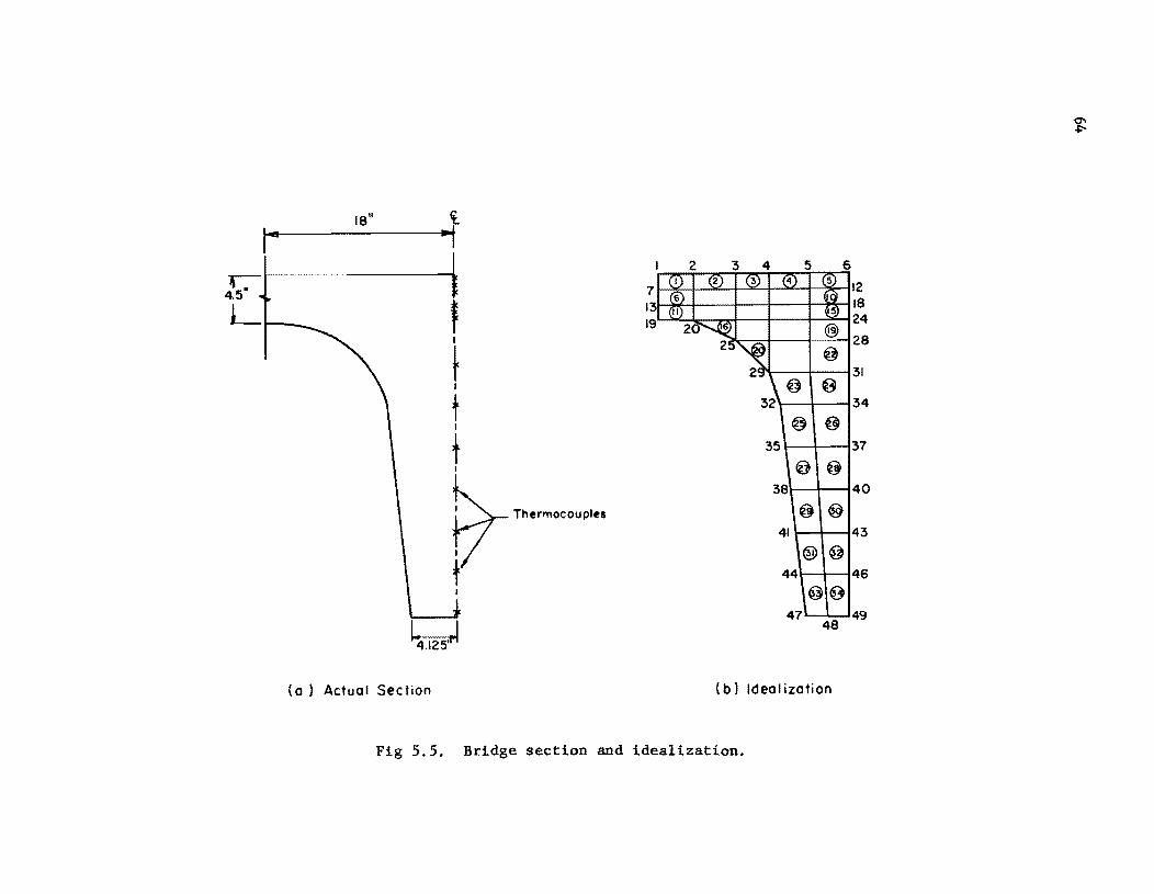
18" i I" .. ,
.-::-4.5 7 12
L __ f 18 24 19' v Is:: u I 'S'
1
t I
t I
t I
~ V Th"moeou,Ie,
t
28
31
34
37
@ ~ 38 40
@ @
41 43
® @
44 46
@~
47' 1 149 48
(0) Actual Section (b) Ideal ization
Fig 5.5. Bridge section and idealization.
~

65
TABLE 5.2 Field Test on August 8, 1967 (Ref 48)
Ambient Ambient Time Tern!:! ~B}* TemE {T2* Remarks
0600 Power turned on for instrument warm-up
0630 78°F 78°F Clear sky - Light wind
0800 79°F 80°F II
0930 80°F 82°F " 1100 86°F 91°F II
1230 90°F 95°F " 1400 95°F lOO°F " 1530 97°F 97°F II
1700 99°F 103°F II
1830 98°F 104°F " 2000 94°F 97°F "
*Ambient Temp (B) - Temperature taken with a mercury bulb four inches from the ground in the shade under the bridge.
Ambient Temp (T) - Temperature taken with a thermocouple one inch above the surface of the bridge.
" 11
" II
II
11
" 11
"
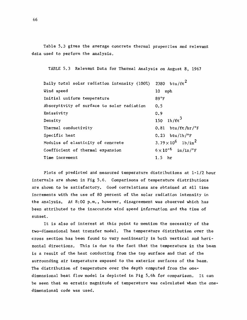
66
Table 5.3 gives the average concrete thermal properties and relevant
data used to perform the analysis.
TABLE 5.3 Relevant Data for Thermal Analysis on August 8, 1967
Daily total solar radiation intensity (100%) 2380 btu/ft 2
Wind speed 10 mph
Initial uniform temperature 89°F
Absorptivity of surface to solar radiation 0.5
Emissivity 0.9
Density
Thermal conductivity
Specific heat
Modulus of elasticity of concrete
Coefficient of thermal expansion
Time increment
150 1b/ft3
0.81 btu/ft/hr/oF
0.23 btu/1brF
3.79 X 10⁶ 1b/in2
6 X 10⁻⁶ in/inrF
1.5 hr
Plots of predicted and measured temperature distributions at 1-1/2 hour
intervals are shown in Fig 5.6. Comparisons of temperature distributions
are shown to be satisfactory. Good correlations are obtained at all time
increments with the use of 80 percent of the solar radiation intensity in
the analysis. At 8:00 p.m., however, disagreement was observed which has
been attributed to the inaccurate wind speed information and the time of
sunset.
It is also of interest at this point to mention the necessity of the
two-dimensional heat transfer model. The temperature distribution over the
cross section has been found to vary nonlinearly in both vertical and hori
zontal directions. This is due to the fact that the temperature in the beam
is a result of the heat conducting from the top surface and that of the
surrounding air temperature exposed to the exterior surfaces of the beam.
The distribution of temperature over the depth computed from the one
dimensional heat flow model is depicted in Fig 5.6h for comparison. It can
be seen that an erratic magnitude of temperature was calculated when the one
dimensional code was used.
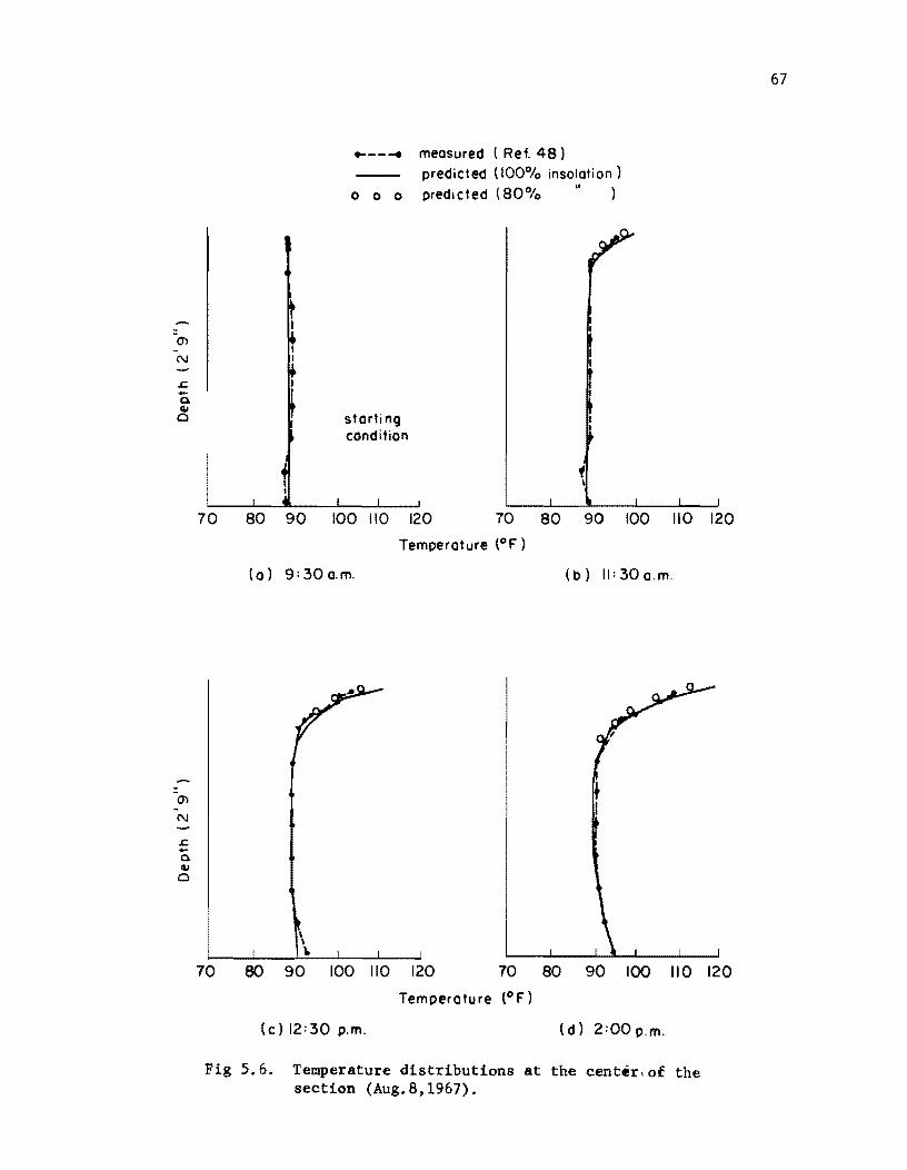
-N
.c. -0. <II o
.c. -0. <II o
... --.... measured (Ref. 48 ) predicted (100% insolation)
" o 0 0 predicted (80% )
storting condition
70 80 90 100 110 120 70 80 90 100 110 120
70
(0) 9:30a.m .
\
"
Temperature (OF)
(b) 11:30a.m.
80 90 100 110 120 70 80 90 100 110 120
Temperature (OF)
(c) 12:30 p.m. (d) 2:00p.m.
Fig 5.6. Temperature distributions at the center<of the section (Aug.8,1967).
67
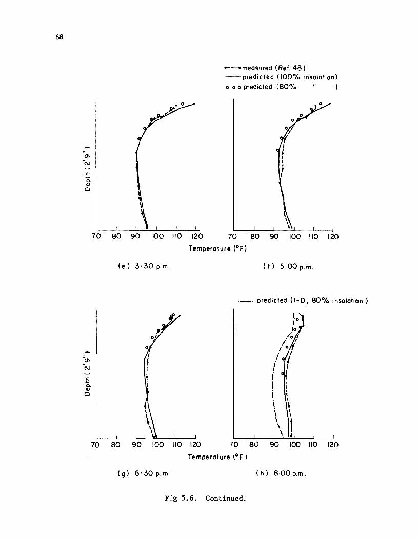
68
.s::; -0. III Cl
.s::; -0. III Cl
--"measured (Ref. 48 ) --predicted (100% insolation) o 00 predicted (80% " )
~ \ \ I J
70 80 90 100 110 120 70 80 90 100 110 120
Temperature (oF)
(e) 3: 30 p. m. (f) 5:00 p.m .
. _. predicted (1-0, 80% insolation)
I I , I , \
t 4
70 80 90 100 110 120 70 80 90 100 110 120
Temperature (OF)
(g) 6:30 p.m. (h) 8:00p.m.
Fig 5.6. Continued.
69
Deflection at the mid-span of the bridge caused by temperature differen
tials was also measured at 1-1/2 hour intervals. Predicted deflections were
obtained by the method described in Chapter 4. Comparisons between the
measured and predicted deflections are depicted in Fig 5.7. No theoretical
results from Ref 48 were available for this comparison. The bridge deflects
upward because the top surface is warmer than the bottom surface. Although
the correlation is not as good as in the temperature distribution case,
shapes of deflection have basically the same trend. Both predicted and mea
sured deflection have approximately the same orders of magnitude. It is
worth noting that the computed deflections are, theoretically, independent
of the modulus of elasticity of the concrete. Thus, the discrepancy of
results in Fig 5.7 is believed to be due to the deviation of the actual
boundary conditions from the theoretical one and the limited one-dimensional
response of the bridge which was assumed in the analysis.
Temperature induced stresses were also computed by the author based on
the one-dimensional elastic beam theory, since the bridge under consideration
has no complicating factors such as skew or irregularities of beam spacing.
Predicted stress distributions over the beam depth are depicted in Fig 5.8a.
It should be pointed out that the temperature induced stresses in this case
are due only to the nonlinearity of the temperature. Compressive stresses
are found at the top and bottom regions while tensile stresses are found in
the vicinity of the neutral axis of the beam with a maximum value of 182 psi.
5.3.2 Temperature Prediction on December II, 1967
During the winter, tests were performed on 10 December 1967 at 5:00 a.m.
and continued until 3:00 p.m. of the next day. Table 5.4 gives ambient air
temperatures and a brief description of the weather conditions during the
field measurements. The initial condition was selected in the same manner
as described earlier, thus the starting time at 9:00 p.m. was used with the
initial uniform temperature distribution 43°F, Fig 5.9a. Table 5.5 gives
the data which was used in the analysis.
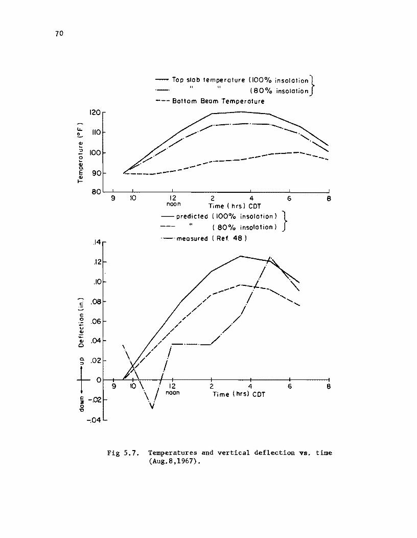
70
120
lL. 110 2...-41 .... :::I 100 -0 .... 41 0. E 41
90 t-
80
.14
.12
.10
c .08
c 0 - .06 u ~ - .04 41 0
0. .02 :::I
t 0
i -.02 0 "t)
-;04
- Top Slob 'empero'"e 1100% InsolOHon} '-' " II (80°10 insolation
--- Bottom Beam Temperature
9 10 12 2 4 6 8 noon Time ( hrs) CDr
-- predicted (100% insolotion) } " ( 80% insolotion)
._. meosured ( Ref. 48)
9 12 2 4 6 8 noon Time (hrs) CDr
Fig 5.7. Temperatures and vertical deflection VB, time (Aug.8,1967).

N.A.
-- 80% insolation
--- 100% insolation
-300 -100 0 100 300
compression tension
(a) 5: 00 p. m. (Aug. 8,67)
-<7'
N -J: -0. ., o
Stress (psi)
71
N.A.
-200 o 200 compression tension
(b) 6: 00 a.m. (Dec. II, 67)
Fig 5.8. Temperature induced stresses.
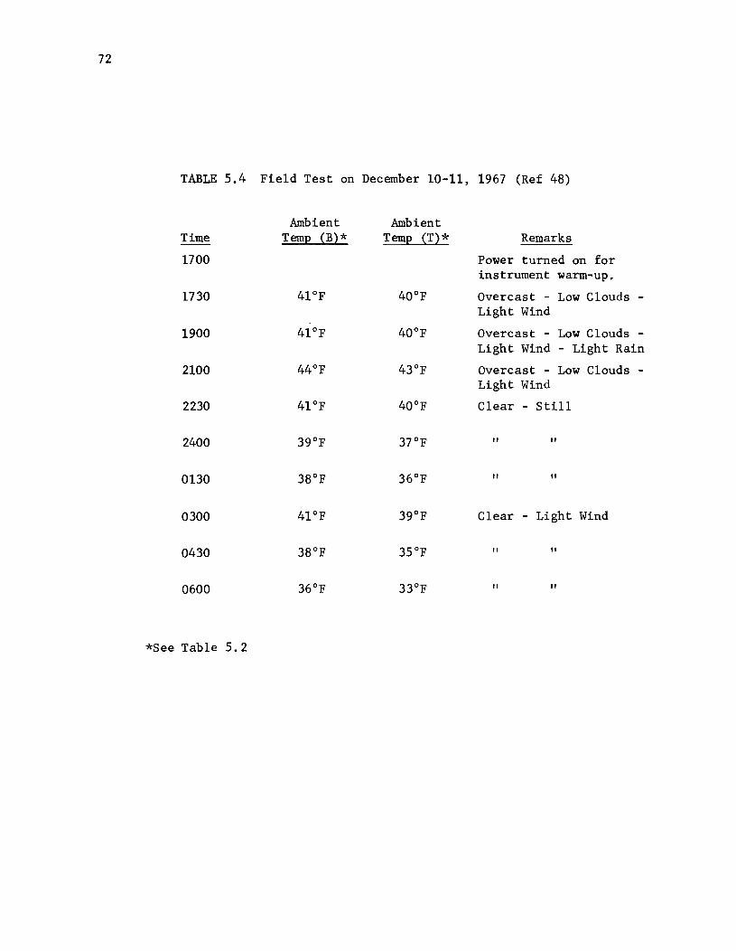
72
TABLE 5.4 Field Test on December 10-11, 1967 (Ref 48)
Ambient Ambient Time TemE {B}* TernE {T}* Remarks
1700 Power turned on for instrument warm-up.
1730 41°F 40°F Overcast - Low Clouds -Light Wind
1900 41°F 40°F Overcast - Low Clouds -Light Wind - Light Rain
2100 44°F 43°F Overcast - Low Clouds -Light Wind
2230 41°F 40°F Clear - Still
2400 39°F 3rF " "
0130 38°F 36°F " "
0300 41°F 39°F Clear - Light Wind
0430 38°F 35°F " "
0600 36°F 33°F " "
*See Table 5.2
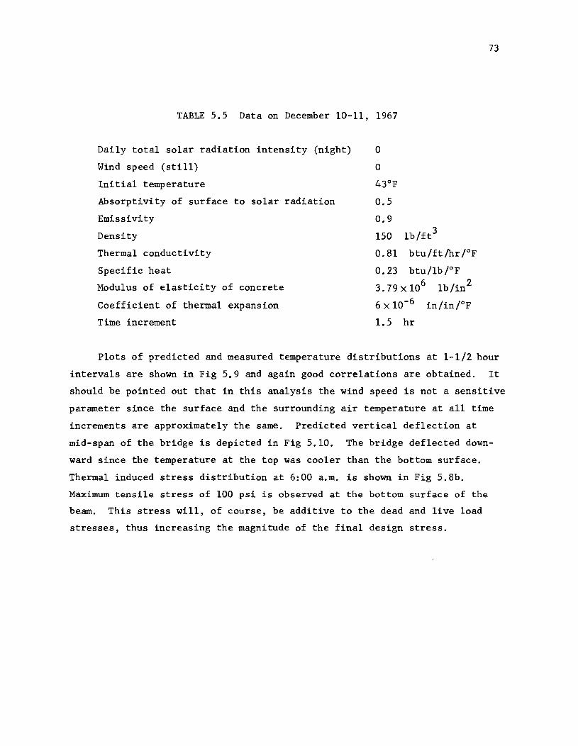
TABLE 5.5 Data on December 10-11, 1967
Daily total solar radiation intensity (night)
Wind speed (still)
Initial temperature
Absorptivity of surface to solar radiation
Emissivity
Density
Thermal conductivity
Specific heat
Modulus of elasticity of concrete
Coefficient of thermal expansion
Time increment
0.5
0.9
150 lb/ft3
0.81 btu/ft/hrrF
0.23 btu/lbrF
3.79Xl06 lb/in2
6 X 10⁻⁶ in/inrF
1.5 hr
73
Plots of predicted and measured temperature distributions at 1-1/2 hour
intervals are shown in Fig 5.9 and again good correlations are obtained. It
should be pointed out that in this analysis the wind speed is not a sensitive
parameter since the surface and the surrounding air temperature at all time
increments are approximately the same. Predicted vertical deflection at
mid-span of the bridge is depicted in Fig 5.10. The bridge deflected down
ward since the temperature at the top was cooler than the bottom surface.
Thermal induced stress distribution at 6:00 a.m. is shown in Fig 5.8b.
Maximum tensile stress of 100 psi is observed at the bottom surface of the
beam. This stress will, of course, be additive to the dead and live load
stresses, thus increasing the magnitude of the final design stress.
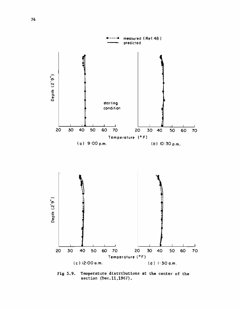
74
-0'1
(\J
~ -a. QI
Cl
.. ---... measured (Re f. 48 ) predicted
starting condition
20 30 40 50 60 70 20 30 40
Temperature (0 F)
50 60 70
(a) 9:00 p.m. (b) 10:30 p.m.
20 30 40 50 60 70 20 30 40 50 60 70 Temperatu re (0 F)
(c ) 12:00 a.m. (d) 1:30 a.m.
Fig 5.9. Temperature distributions at the center of the section (Dec.ll,1967).
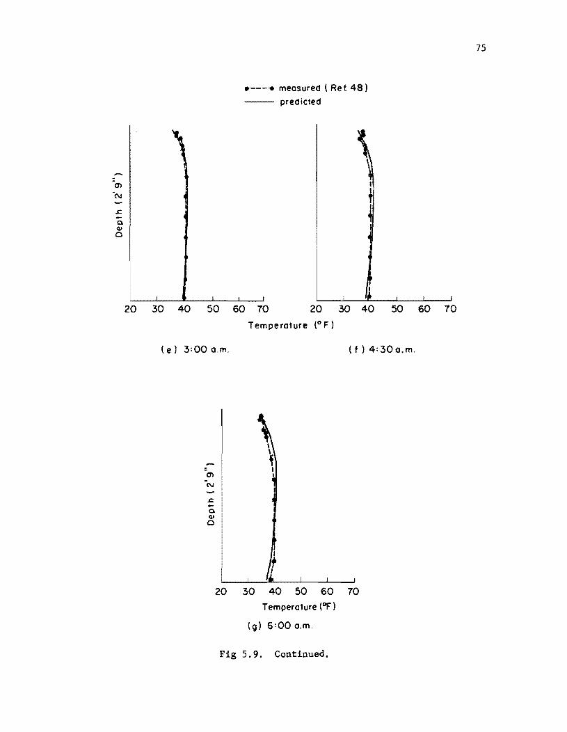
s::. -a. CLJ o
tt---" measured ( Re { 48)
-- predicted
20 30 40 50 60 70 20 30 40 50 60 70
Temperature (0 F)
(e) 3:00 a.m. (f) 4:30a.m.
s::. -a. CLJ o
20 30 40 50 60 70
Temperature (Of')
(9) 6:00 a.m.
Fig 5.9. Continued.
75

76
LL. 2.-QJ ... :J -0 ... QJ 0. E QJ t-
0. :J
r:: t c 0
u c QJ ~
0 QJ
't:J
0
4
40
35
_ _ r Bottom beam temperature ---~---- -...-....-.--~-... -----..------ -.......
Top Sia b temperature
30
a) Surface temperatures
.02 midnight
9 10 12 2 4 6 Time (hrs) CST 0
-.02
-.04 predicted
b} Bridge deflection
Fig 5.10. Temperatures and vertieal deflection vs. time (Dec. 11,1967).
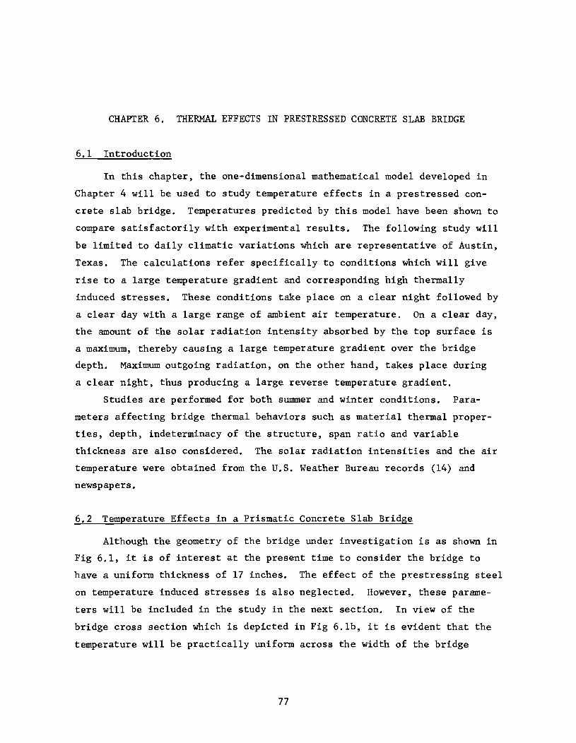
CHAPTER 6. THERMAL EFFECTS IN PRESTRESSED CONCRETE SLAB BRIDGE
6.1 Introduction
In this chapter, the one-dimensional mathematical model developed in
Chapter 4 will be used to study temperature effects in a prestressed con
crete slab bridge. Temperatures predicted by this model have been shown to
compare satisfactorily with experimental results. The following study will
be limited to daily climatic variations which are representative of Austin,
Texas. The calculations refer specifically to conditions which will give
rise to a large temperature gradient and corresponding high thermally
induced stresses. These conditions take place on a clear night followed by
a clear day with a large range of ambient air temperature. On a clear day,
the amount of the solar radiation intensity absorbed by the top surface is
a maximum, thereby causing a large temperature gradient over the bridge
depth. Maximum outgoing radiation, on the other hand, takes place during
a clear night, thus producing a large reverse temperature gradient.
Studies are performed for both summer and winter conditions. Para
meters affecting bridge thermal behaviors such as material thermal proper
ties, depth, indeterminacy of the structure, span ratio and variable
thickness are also considered. The solar radiation intensities and the air
temperature were obtained from the U.S. Weather Bureau records (14) and
newspapers.
6.2 Temperature Effects in a Prismatic Concrete Slab Bridge
Although the geometry of the bridge under investigation is as shown in
Fig 6.1, it is of interest at the present time to consider the bridge to
have a uniform thickness of 17 inches. The effect of the p~estressing steel
on temperature induced stresses is also neglected. However, these parame
ters will be included in the study in the next section. In view of the
bridge cross section which is depicted in Fig 6.1b, it is evident that the
temperature will be practically uniform across the width of the bridge
77
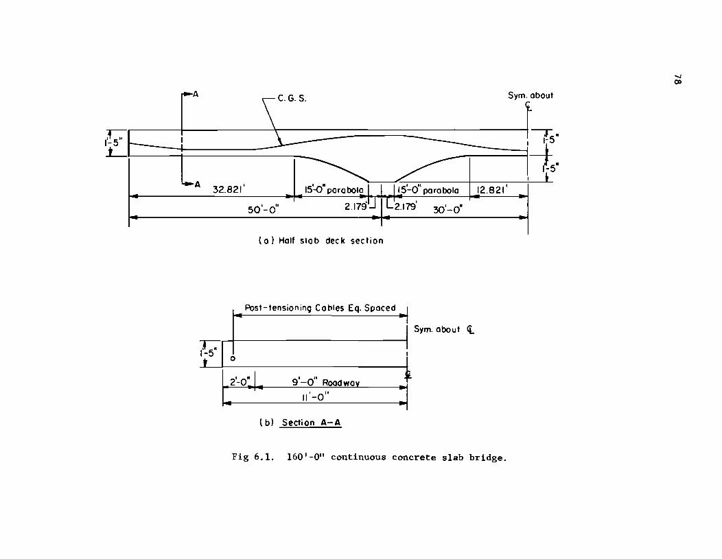
A Sym. about
[F E ======:; !=r: 1-5
A 32.821' 15~· parabola 12.821'
50'-0" 2.179 30'-0·
ta) Half slab deck section
Post-t Cables Ea. S d
i Sym. about <t
~ ! I-i 0
2'-0· _I 9'-0" Roadway
II '-0" -
t b) Section A-A
Fig 6.1. 160' -0" continuous concrete slab bridge.
-../ 00
79
except for the regions near the ends. Consequently, the bridge was analyzed
by assuming the temperature to vary one-dimensionally over the depth. Also
the bridge was assumed to have orthogonal supports.
6.2.1 Sensitivity Analysis of the Model
The purpose of this study was to detect the significant factors that
affect the bridge thermal behaviors subjected to daily environmental
changes. In doing so, eight variables were considered: daily total inso
lation intensity, surface absorptivity, thermal conductivity, specific heat,
unit weight, wind speed, thickness and the range of daily air temperature.
Weather variables which are representative of August were used. Material
thermal properties selected are typical for a normal weight concrete. These
values are listed in Table 6.1 for future references.
In the analysis a starting time at 7:00 a.m., which is approximately
one hour after sunrise, was used. This selection was made due to past
experiences which indicated that temperatures in a bridge would be rela
tively uniform at or a few hours after sunrise with a value equaling the air
temperature at that time. Consequently, an initial uniform temperature
distribution of 78°F was used. The analysis was performed for a complete
24 hour period with a time increment of 15 minutes.
Temperature distributions and stresses were calculated, using the data
given in Table 6.1. The predicted results are also listed in Table 6.1.
By keeping the rest of the variables at their average values, one variable
at a time was increased by 10 percent and the temperatures and stresses
were computed. A summary of comparisons of the maximum surface temperature
and the maximum temperature gradient, etc., is given in Table 6.2. It can
be seen that the most significant factor with respect to the material
thermal properties is the absorptivity of the surface to the solar radiation.
Also of importance is the coefficient of thermal expansion and contraction,
since the thermal induced stresses vary linearly with this variable. How
ever, an increase in the thermal conductivity, specific heat and density
reduces the temperature gradient and thus decreases the induced stresses.
With respect to the environmental variables, an increase in the solar
radiation intensity and the daily air temperature range amplifies the pre
dicted temperature gradient and the temperature induced stresses. An

80
TABLE 6.1 SELECTED AVERAGE VALUES FOR THE SENSITIVITY ANALYSIS (AUGUST)
Average total insolation intensity
Air temperature distribution
Wind speed
Absorptivity of surface to solar radiation
Emissivity
Thermal conductivity
Specific heat
Unit weight
Depth
Modulus of elasticity of concrete
Coefficient of thermal expansion
2380
Fig
10
0.5
0.9
0.81
0.23
150
17
3.2a
4.25 X 10⁶
6.0xlO-6
PREDICTIVE RESULTS (3-equal-span-bridge)
Maximum top surface temperature 120
Maximum temperature gradient 30
Maximum reverse temperature gradient 7
Maximum tensile stress (bottom half) 239
Maximum tensile stress (top) 318
Maximum compressive stress (top) 818
Maximum vertical deflection (downward) 0.125
Maximum mean bridge temperature 35
btu/ft 2
mph
btu/ft /hr ;OF
btu/lb;oF
lb/ft3
inches
lb/in2
in/in;oF
psi
psi
psi
inch
increase in the wind speed, on the other hand, decreases the computed
results. Consequently, the extreme climatic condition is qelieved to
take place on a still day with a maximum value of the solar radiation and
a maximum range of daily ambient air temperature.
Comparisons of predicted results using different variations of solar
intensity are also given in Table 6.2. By keeping the total insolation in

Average
Insolation
Absorptivity
Conductivity
Specific heat
Density
Wind speed
Thickness
Range of air temperature
Insolation (Eq 3.1)
-
TABLE 6.2 THE EFFECTS OF A 10% INCREASE IN ONE, VARIABLE AT A TIME ON TEMPERATURES AND STRESSES IN A THREE EQUAL SPAN CONCRETE SLAB BRIDGE (AUGUST)
Temp. Temp. Tensile Compo Reverse Tensile Vertical (top) gradient stress stress gradient stress(top) deflection
0% 0% 0% 0% 0% 0% 0%
2.5 10 9.2 8.1 0 1.6 9.6
2.5 10 9.2 8.1 0 1.6 9.6
-0.8 -3.3 -0.8 -3.3 0 -2.5 -0.8
-0.8 -3.3 - 2. 9 -0.1 0 - 2. 5 -2.4
-0.8 -3.3 - 2.9 -0.1 0 -2.5 -2.4
-0.8 -3.3 -2.1 -1.5 0 0 -2.4
0 0 -0.8 3.3 0 -0.3 -11. 2
1.7 0 2.1 3.1 14.3 4.7 0.8
3.3 13.3 9.2 11.4 0 0.3 10.4 - -
Mean bridge temp.
0%
2.9
2.9
0
- 2.9
- 2.9
0
-5.7
2.9
-0.3 -
I
I
co I-'

82
a day the same, Eq 3.1, instead of Eq 3.2, was used in the analysis. Two
distributions of solar intensity computed from these two equations have
been shown in Fig 3.1. It can be seen, from Table 6.2, that larger tempera
ture stresses were predicted when Eq 3.1 was used.
6.2.2 A Study on Initial Conditions
Be£ore the bridge temperature distributions can be predicted the
initial condition must be specified. This condition includes the reference
time and the initial temperature distribution. A study of a typical daily
solar radiation and air temperature variation indicates that the temperature
in a bridge will be relatively uniform early_in the morning. At about this
time, the sun's radiation is small and the air temperature has just passed
the minimum value. It should be pointed out that bridges subjected to daily
atmospheric variations may not have an exact thermal equilibrium condition,
thus it was the purpose of this study to investigate the response of the
temperature distributions and stresses caused by different initial
conditions.
Computed temperature and stress distributions using different reference
times and different initial temperature variation are depicted in Fig 6.2.
The initial temperature distribution was assumed to be uniform and equal
to the surrounding air temperature at the selected reference time. The
analyses were made at 15 minute intervals using the data contained in Table
6.1. It is found that maximum interior tensile stresses occurred at 3:00
p.m. while maximum reverse stresses occurred at 5:00 a.m. FromrFig 6.2,
it is evident that different starting conditions do not have significant
effects on the temperature induced stresses. According to the assumed
initial conditions at 7:00 a.m., the following results were observed. At
3:00 p.m., a maximum tensile stress of 239 psi is located at three-fourth's
of the bridge depth. At the bottom surface, the tensile stress is much
smaller, i.e., 97 psi. A maximum temperature gradient took place at 2:00
p.m. and the corresponding maximum compressive stress is 818 psi at the top
fiber of the bridge. At 5:00 a.m., on the other hand, a maximum reverse
temperature gradient was calculated with a maximum tensile stress of 318
psi at the top surface, Fig 6.2b.
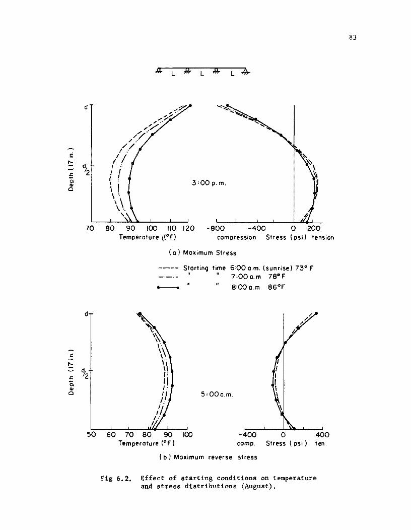
.S I'-
.r:. -0. ClI
0
d
d;. 2
L L
,,-::. ..... ~
" "
~
",/,,: //,"
/ " ,</ /1 I :
I I \ I 3:00p.m.
\ '.
\ \ , '. ,
L A-
70 80 90 100 110 120 - 800 -400 o 200 compression Stress (psi) tension
(a) Maximum Stress
Starting time 6:00 a.m. (sunrise) 73° F II "7:00a.m 780F
• • .. 8:00o.m 86°F
d
.r:. <12 -0. ClI o 5:00a.m.
50 60 70 80 90 100 -400 o 400 Temperature (OF) compo Stress (psi) ten.
( b ) Maximum reverse stress
Fig 6.2. Effect of starting conditions on temperature and stress distributions (August),
83
84
The above stresses were computed at the center of the middle span.
However, it should be pointed out that, in this three-span case, the
temperature induced stresses are constant longitudinally in the middle
span. In the exterior spans, the stresses reduce linearly such that zero
stress is computed at the exterior ends.
The determination of temperature and stresses caused by the same envi
ronmental conditions which are repeated over a period of several days is
also of interest. In this study, the daily climatic changes as recorded
in August and January were considered. Figure 6.3a depicts temperature and
stress distributions at 3:00 p.m. in August. On the first day, the thermal
equilibrium was assumed to take place at 7:00 a.m. and calculations pro
ceeded for three consecutive days. It can be seen from Fig 6.3a that during
the first day additional heat is stored within the bridge, thus decreasing
the nonlinearity of the temperature distribution. This gain of heat, how
ever, reduces considerably during the second day and a isothermal condition
is observed on the third day. The changes of stress distribution, on the
other hand, are found to be relatively small. Stresses computed at the
center of the middle span are also shown in Fig 6.3a. According to the
above analyses, it is evident that the system will stabilize itself at
8:00 a.m., i.e., if a starting condition at 8:00 a.m. is used the bridge
will reach an equilibrium condition with the environment at this time on the
next day. This conclusion is clearly illustrated by comparing plots in
Fig 6.2a and Fig 6.3a.
Temperature and stress distributions at 7:00 a.m. in January are
depicted in Fig 6.3b. The plots shown are those giving the maximum reverse
temperature differential and the maximum stresses. The distribution of air
temperature used in the analysis is shown in Fig 3.2b. The initial con
dition was assumed to occur at 8:00 p.m. with a uniform temperature of 65°F.
This time was selected since experimental data (20,48) have shown that
during the winter period the temperature distribution over the depth is
relatively uniform at about this time. It can be seen in Fig 6.3 that
changes of temperature between the first and the second day are small and
that computed stresses are almost identical. The maximum reverse gradient
of 9°F was calculated and a maximum tensile stress of 352 psi was predicted
at the top surface.

c:
-0. III o
d
70
d
30
L L L4
3:00 p. m.
80 90 100 110 120 Temperature (0 F)
-800 com pression
-400 o 200
, '" "-\".
(a) August
first day
second day
- third day
'\ \.
\~ \. \" \\ I: q I. ,. 1/ /:
I 7:00 a.m.
40 50 60 70 Temperature (OF)
80 -400 compressi 0 n
( b) January
Stress (psi) tension
/ I
I I I I \ \ \ \ \
I' /
\
o
,/ /
,/
" ,/
Stress (psi)
400 tension
Fig 6.3. Effect of the environmental repetition on temperature and stress distributions.
85

86
The above study thus indicates that different starting times have
little influence on the induced stresses. In the following investigation
the starting time at 7:00 a.m. and 8:00 p.m. will be used for the summer
and winter condition respectively.
6.2.3 A Study on Summer Conditions
It has been shown in Section 6.2.1 that large temperature gradients
occur during a day with high solar radiation, large air temperature range
and no wind. However, although the range of air temperature is found to be
maximum in August, Fig 3.2a, a maximum solar radiation intensity is recorded
in June, Table 3.1. Therefore, in order to study the bridge thermal be
haviors associated with summer daytime conditions, daily climatic changes
in June, July and August needed to be investigated.
Temperature and stress distributions calculated at 4:00 p.m. and 5:00
a.m. are depicted in Fig 6.4. The analyses were performed using the star
ting condition at 7:00 a,m. In addition, a wind speed of 5 mph was used.
The stresses were computed at the center of the middle span. It can be
seen that the changes of the stress distribution are small. A maximum
tensile stress of 270 psi is located at three-fourth's of the depth, Fig
6.4a. At 2:00 p.m" a maximum compressive stress was calculated at the top
surface and is 890 psi. Figure 6.4b shows the predicted maximum reverse
gradients and the stresses. A maximum tensile stress of approximately 310
psi is found at the top surface,
Therefore, it is evident from this study that the daily environmental
variations in August are the extreme summer conditions in Austin, Texas.
Plots of predicted top and bottom surface temperatures versus time in
August are depicted in Fig 6.5a. A maximum difference of 35°F is found
between the top and the bottom temperature at 2:00 p.m. At this time,
the top surface is approximately 20°F warmer than the air temperature.
6.2.4 A Study on Winter Conditions
In contrast to the summer conditions, large reverse temperature
gradients occur during a still night with a maximum amount of outgoing
radiation and a large range of air temperature. In view of these factors,

-Q. CII o
s: -Q. CII o
d
d
60
Temperature (0 F)
Temperoture (0 F)
4:00 p.m.
compression
(a)
_"- June ---- July --- August
5:00 a.m.
(b)
-400 compression
wind speed 5 mph
400 Stress (psi) tension
o 400 Stress (psi) tension
Fig 6.4. Temperature and stress distributions (summer conditions).
87

88
90
BO Lt... ~ QI ... 70 'j -0 ... QI Q.
E QI
50 I-
40
308
12noon
12 midnight
6
wind speed = 5 mph depth = 17 in.
-- Top surface temperature
---- Bottom" "
_._.- Air Temperature (range 34° F)
----
12midnight 6 Time (hrs) CST
(a) August
-'-'- Air Temperature (tange 45° F)
.... ---... ....... ... .-.......
6 12 6 noon
Time (hrs) CST
( b) January
Fig 6.5. Plots of temperatures for a clear day and night.
89
the daily atmospheric variations in December, January and February are used
for this study. The hourly distribution of air temperatures for each of
these months are depicted in Fig 3.2b. The solar radiation intensities, on
the other hand, are listed in Table 3.1.
Temperature and stress distributions calculated at 7:00 a.m. and 3:00
p.m. are shown in Fig 6.6. The starting condition was assumed to take
place at 8:00 p.m. Again, the induced stresses were computed at the center
of the middle span. Figure 6.6a indicates that a maximum tensile stress of
352 psi at the top surface occurs in January. Figure 6.6b, on the other
hand, shows that a maximum tensile stress located at three-fourth's of the
depth occurs in February. This is due to the fact that the solar radiation
intensity in February is higher than that in January, thus producing larger
temperature gradients and consequently higher induced stresses during the
daytime. These stresses, however, are less than those induced under the
summer conditions.
It is, therefore, concluded that the daily climatic changes in January
are the extreme winter conditions in Austin, Texas. Plots of predicted
top and bottom surface temperatures versus time in this month are shown in
Fig 6.5b. A maximum difference of 9°F is found between the top and bottom
temperature at 7:00 a.m. During daytime, the top surface temperature
increases at a somewhat .. faster rate than the air temperature, but the
maximum difference of only 6°F is observed between the two temperatures and
takes place at 2:00 p.m.
6.2.5 Effects of Interior Supports on Temperature Induced Stresses
The indeterminacy of the structure has been known to be one of the
significant sources of thermal induced stresses. The temperature stresses
in a simply supported bridge are due only to the nonlinear temperature
while a continuous bridge share this same stress plus flexural stresses
since the interior supports offer vertical restraint which would take place
due to a temperature differential over the bridge depth.
Temperature induced stresses for a single span statically determinate
bridge and statically indeterminate structures with two and three spans are
shown in Fig 6.7. The stresses were computed at the section of symmetry of
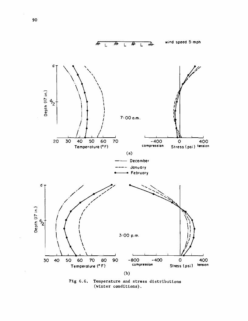
90
d
~
c:: I'-
..c: Q QJ 0
d
dl 2
"\ \
\
.I
\ \ I /
, , , , \ \ \ \
\ \ \ \ \ \ I I I I I
I I
7:00 a.m.
-400 20 30 40 50 60 70 Temperature (OF) compression
I I \
/
\.
.' /
/ /"
(a)
-"- Oecember
---- January
• • February
3:00 p.m.
30 40 50 60 70 80 90 Temperature (0 F)
-800 -400 compression
(b)
wind speed 5 mph
o 400 Stress (psi) tension
o 400 Stress (psi) tension
Fig 6.6, Temperature and stress distributions (winter conditions).
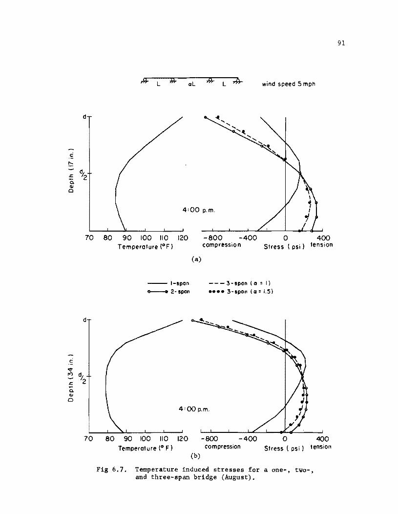
0. ell a
d
70
d
70
L aL LOA- wind speed 5 mph
4:00 p.m.
80 90 100 110 120 Temperature (OF)
-800 -400 o 400 compression Stress ( psi) tension
-- I-span •• --64& 2 - span
(a)
- - - 3 - span (a = I) •••• 3-spon (a: 1.5)
4:00 p.m.
-800 -400 o 400 80 90 100 110 120 Temperature (0 F) compression Stress ( psi) tension
(b)
Fig 6.7. Temperature induced stresses for a one-, two-, and three-span bridge (August).
91
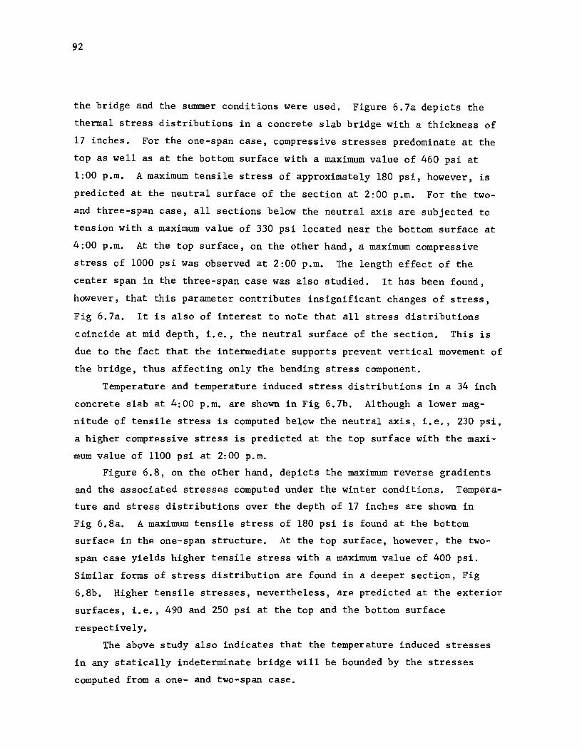
92
the bridge and the summer conditions were used. Figure 6.7a depicts the
thermal stress distributions in a concrete slab bridge with a thickness of
17 inches. For the one-span case, compressive stresses predominate at the
top as well as at the bottom surface with a maximum value of 460 psi at
1:00 p.m. A maximum tensile stress of approximately 180 psi, however, is
predicted at the neutral surface of the section at 2:00 p.m. For the two
and three-span case, all sections below the neutral axis are subjected to
tension with a maximum value of 330 psi located near the bottom surface at
4:00 p.m. At the top surface, on the other hand, a maximum compressive
stress of 1000 psi was observed at 2:00 p.m. The length effect of the
center span in the three-span case was also studied. It has been found,
however, that this parameter contributes insignificant changes of stress,
Fig 6.7a. It is also of interest to note that all stress distributions
coincide at mid depth, i.e., the neutral surface of the section. This is
due to the fact that the intermediate supports prevent vertical movement of
the bridge, thus affecting only the bending stress component.
Temperature and temperature induced stress distributions in a 34 inch
concrete slab at 4:00 p.m. are shown in Fig 6.7b. Although a lower mag
nitude of tensile stress is computed below the neutral axis, i.e., 230 psi,
a higher compressive stress is predicted at the top surface with the maxi
mum value of 1100 psi at 2:00 p.m.
Figure 6.8, on the other hand, depicts the maximum reverse gradients
and the associated stresses computed under the winter conditions. Tempera
ture and stress distributions over the depth of 17 inches are shown in
Fig 6.8a. A maximum tensile stress of 180 psi is found at the bottom
surface in the one-span structure. At the top surface, however, the two
span case yields higher tensile stress with a maximum value of 400 psi.
Similar forms of stress distribution are found in a deeper section, Fig
6.8b. Higher tensile stresses, nevertheless, are predicted at the exterior
surfaces, i.e., 490 and 250 psi at the top and the bottom surface
respectively.
The above study also indicates that the temperature induced stresses
in any statically indeterminate bridge will be bounded by the stresses
computed from a one- and two-span case.
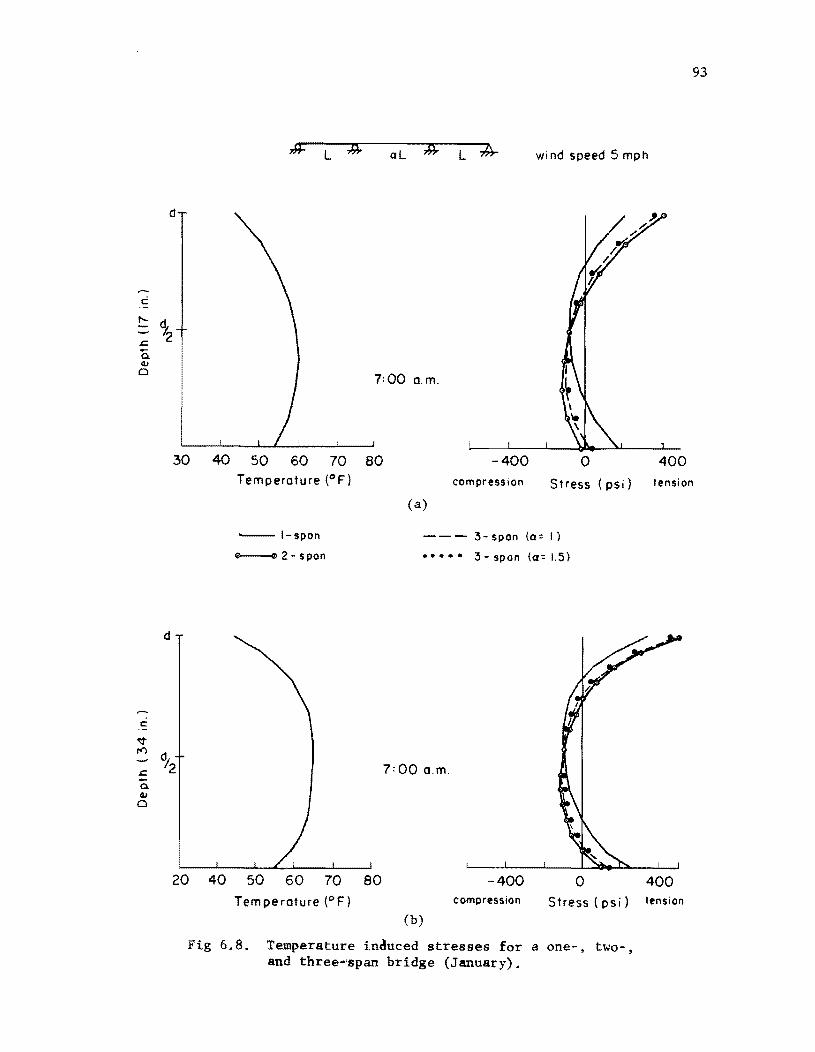
L '4 aL L "A- wind speed 5 mph
d
7:00 o.m.
30 40 50 60 70 80 -400 0 400 Temperoture (OF) compression Stress ( psi) tension
(a)
-I-spon --- 3-span (a = I)
G>-----f> 2 - s po n ••••• 3-spon (a=1.5)
7:00 a.m.
-400 o 400 20 40 50 60 70 80 Temperature (OF) compression Stress (psi) tension
(b)
Fig 6.8. Temperature induced stresses for a one-, two-, and three"'span bridge (January).
93

94
6.2.6 Effects of Longitudinal Restraining Forces on Temperature Induced Stresses
In the preceding studies, the stresses were calculated based on the
assumption that the bridge was unrestrained longitudinally. In general, as
a thermal movement occurs, restraining forces are developed at the supports,
thus yielding another set of stresses. For a friction bearing, the trans
lational force will be transmitted directly to the support until the
magnitude of thermal force equals ~R, where ~ is the coefficient of
friction which normally depends on the type of the bearing, corrosion of
the bearing, etc. The reaction R must also include the additional
reaction change caused by a temperature differential in the bridge.
Consider a simply supported concrete slab bridge 60 ft long and 17
inches deep. If the bridge temperature is raised uniformly lOF above the
temperature representative of the thermal equilibrium condition, the amount
of force which is required to prevent the longitudinal movement will be
5200 lb. The friction force at the support, on the other hand, is only
1280 lb with ~ equal to 0.2. Since the thermal force is greater than the
friction force, movement occurs. According to the author's analyses, the
stresses caused by this restraining force have been found to be insignifi
cant because the computed maximum stress is only 8 percent of the maximum
unrestrained temperature induced stress.
6.2.7 A Study on Polynomial Interpolation
The study was made in order to select a mathematical function which can
represent the shapes of the temperature distribution as well as the shapes
of the temperature induced stress in the concrete str~cture. In doing so,
two types of polynomial interpolation were investigated. They are second
and fourth-order polynomials. Comparisons of results are given in Fig 6.9.
It can be seen that the quartic function has superior representation com
pared to the quadratic function in fitting the predicted temperature and the
stress distribution. Although the quadratic function gives good results for
the depth of l7 inches, Fig 6.9a, poor results, .however, are observed for the
depth of 34 inches, Fig 6.9b.

s: -0. CI.! o
d
3:00p.m.
70 80 90 100 110 120 Temperature (OF)
(a)
predicted
• • • quartic
quadratic
-800 compression
-400 o 200 Stress ( psi) lension
d
,;'
/" /
I I
I
;' ;'
/'
"" /'
!>.
\
12 :00 nOOn
\ \ ,
,/
I I
I I
I
70 80 90 100 110 120 Temperature (0 F)
-800 -400 0 200 compression Stress ( psi) tension
( b)
Fig 6.9. Representative polynomial interpolations for temperature distributions.
95

96
It has been shown, therefore, that.· the bridge'i:emperatureldd..sttibl1tion
at· any time can be reproduced.by:knowing the temperature at 5 locations
over the depth. An in depth studyo£ the., t,emperature induced stresses
can now be mafl'et• Figurce..~6,. 10" depicts the decomposition of a' given .tem
perature distribution into. each component of the fourth-order poilynomial
interpolation. Stresses at exterior surfaces computed from each £ompon~nt
of temperature gradient are also shown in Fig 6.10. It can be seen that the
linear and the cubic stress components depend on the span ratio, thus
affecting the flexural stress. The linear stress component, however, will
vanish if a one-span bridge is being considered while the cubic stress
component will yield a certain amount of induced stresses. The quadratic
and the quartic stress components, on the other hand, are independent of
the span ratio, thus affecting only the axial stress. It should be noted
that these two stress components always exist even for the statically
determinate bridge. The method presented herein can then be easily used
in estimating the temperature induced stresses.
6.3 Temperature Effects in a Non-Prismatic Concrete Slab Bridge
Temperature effects in the concrete slab bridge, as shown in Fig 6.1,
studied so far assumed that the bridge had a uniform thickness throughout
its length. To take into account the varying section, an approximate
analysis is employed herein. In this method the bridge is divided into a
number of beam elements. Each element has a constant depth as shown in
Fig 6.11. If the prestressing steel effect is neglected, the equivalent
end forces of each beam element due to changes of temperature can be
computed by the method discussed earlier. Since these beam elements are
connected at nodal points, net forces will be left over at points where
adjacent elements have different thicknesses. Stresses caused by these
forces can then be calculated by using the stiffness method. To obtain the
temperature induced stresses, stresses computed from the clamped condition
are superimposed upon the above stresses. Comparisons of results are given
in tabular form in Fig 6.12a. It can be seen that a change of approximately
15 percent is observed for the maximum tensile stress.
Z
L
M I F! _m~ I ~ ~ p = p
eq -c:;- '"" L ;g;:: /3LI2 1 ~ ~ ~ \. M~ - Meq ( 3/3 + 2)
/3 = span ratio (3-span) = 0 (2-span)
= -I (I-span)
d/2~T' d/4 T2
o T,
-d/4 T. -d/Z T~
6To
= o +
6T,
1 +
6T2
[ + ! + r T(Z) E OZ ez2 az '
1= + \ + ) + l +
stress @ I£. 0 -O"T = 0"8 O"T= 0"8 -O"T'"O"a
= 3 (/3+ I) Ea6T. = -2Ea6Ti! '" ('38+ 2.6) Ea6T,
3/J+2 '3 3/3+ 2
OM= Ea6 Ta
3
Fig 6.10. Fo~rth order polynOmial components representing temperature and stress distributions.
AZ·
] O"T =0"8
= - 4 Ea6T.
5
0" .. = Ea6T.
5
\0
"

(a) Bridge elevation
i
t CD ® 0 @) ® ~@ @ ® ! ~ It ~ 3 .4 5 6 7 8 Ii- 10 Ii 12 13 14 i 15
I 9 I (b) Beam element idealizotion
Fig 6.11. Prestressed non-prismatic concrete slab bridge and the idealization.
\0 00
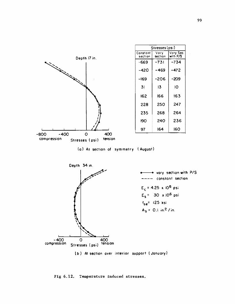
Stresses (psi) Constant Vary Vary Sec.
Depth 17 in. section section with PIS
-669 -731 -734
-420 -469 -472
-169 -206 -209
31 13 10
162 166 163
228 250 247
235 268 264
190 240 236
97 164 160 -800 -400 o 400
compression Stresses (PSi) tension
(a) At section of sym met r y (August)
Depth 34 in.
-400 0 400 compression Stresses (psi) tension
• • vary section with PIS
constant section
E c = 4.25 x. 106 psi
Es = 30 x 106 psi
fse= 125 ksi
As = 0.1 ;n,2 I in.
(b) At section over interior support (January)
Fig 6.12. Temperature induced stresses.
99
100
If the steel tendon is considered in the stress analysis, an additional
restraining force at the location of the steel must be taken into account.
This force is induced due to the strain compatibility requirement since
concrete and steel have a different coefficient of thermal expansion and
contraction. In computing this restraining force, it is assumed that the
temperature in the tendon is the same as the temperature of the surrounding
concrete. The derivation of this force can be found in Appendix D. The
temperature induced stresses are then obtained by the same procedure
mentioned above. Comparisons of stresses are shown in Fig 6.l2a and b.
Also, in the table of Fig 6.l2a, the effect of the prestressing steel on
temperature induced stresses is found to be very small. This is due to the
fact that the difference of the coefficient of thermal expansion between
steel and concrete is small.
6.4 Summary
It can be seen from the foregoing studies that the daily climatic
changes introduce nonlinear temperature distributions in concrete structures.
These temperature variations over the depth can be approximately represented
by a fourth-order polynomial interpolation. During a hot summer day, a
maximum temperature differential between the top and the bottom surface of
35°F 1s possible. At this time, the top surface will be about 20°F warmer
than the air temperature. On a cool winter morning, however, a maximum
reverse temperature gradient is only 9°F.
With regard to longitudinal movements of the bridge, the calculated
maximum and minimum mean bridge temperatures are approximately 35°F and
40°F respectively. These values were computed by assuming the bridge
temperature at the time of erection was 60°F. Consequently, on a cool
winter morning, a thermal strain of 240 millionths is predicted. This
compares with a shrinkage strain of 200 millionths suggested in the AASHO
Specifications. The specifications, however, suggest the maximum and the
minimum mean bridge temperatures to be 3QoF and 4QoF respectively.
The computed thermal deflections are small. The thermal induced
stresses, on the other hand, appear to be significant. Analyses of

101
temperature stresses in a typical continuous concrete slab bridge indicate
that on a typical hot summer afternoon the top surface may experience com
pressive stresses close to 1000 psi. These stresses, therefore, represent
about 50 percent of the allowable compressive stress for concrete. Also,
interior tensile stresses of approximately 330 psi are predicted at
locations below the neutral surface of the section, thus accounting for
about 60 percent of the modulus of rupture for concrete. On a typical cool
winter morning, however, top surface tensile stresses of about 400 psi are
possible.

CHAPTER 7. THERMAL EFFECTS IN COMPOSITE BRIDGES
7.1 Introduction
The problem of thermal effects in composite structures has been studied
by many researchers. In the past, due to the lack of the mathematical nature
of temperature distribution within the composite bridges, temperature induced
stresses were computed based on assumed temperature variations over the
bridge section. Temperature distributions such as a uniform, linear and
parabola (4,35,57) were commonly assumed. Stress results thus obtained can
then be either too high or too low. Field measurements of temperature in
existing composite steel bridges are, therefore, being undertaken in many
places to determine actual bridge temperature distributions. Obviously, this
involves a lot of time and labor. Another means of obtaining bridge tempera
ture distributions is by an analytical approach.
In Chapter 4, a two-dimensional mathematical model was developed for
predicting bridge temperature distributions. The application and the validity
of the model has been verified in Chapter 5. Based on good correlations
between the predicted and the measured bridge temperatures in a typical pan
type reinforced concrete bridge, it is felt that temperature variations in
various types of highway bridges can be estimated in a systematic way. In
this chapter, investigations of temperature effects will be performed for
two types of composite bridges, i.e., a precast pretensioned concrete beam
reinforced concrete slab and a,stee1 beam-reinforced concrete slab bridge.
Daily environmental conditions recorded in the city of Austin, Texas will be
used in these studies.
In addition, the study of temperature effects in a narrow bridge struc
ture is also included in this chapter. This type of bridge was selected
since it inherits the complexities due to side heating of the girders and
shading of the slab by the parapet. The bridge was analyzed under thermal
loading using measured surface temperatures. The study was intended to
compare the measured effects with the results computed from theoretical
considerations employing the one-dimensional beam behavior.
103

104
7.2 Composite Precast Pretensioned Bridge
A typical interior girder, Texas standard type-B, of a composite precast
pretensioned bridge is shown in Fig 7.1. The bridge is made continuous for
live load by placing reinforcing steel in the slab over the piers. The beam
spacing is 8 ft center to center with a cast-in-p1ace concrete slab of 6.5
inches thick. The finite element mesh has a total number of 90 elements with
117 nodal points. Triangular as well as rectangular elements are used to
represent the true I-shape of the beam cross section. The effect of pre
stressing steel on thermal induced stresses is not considered as it has been
shown in the previous chapter that this effect on final stresses is small.
The concrete thermal properties which were used are given in Table 6.1. The
compressive strength of the concrete slab and beam are 3000 and 6000 psi
respectively.
7.2.1 Temperature Effects on a Warm Sunny Day
Temperature distribution at 3:00 p.m. on a warm sunny day, in the month
of August, is depicted in Fig 7.2a. August was selected since it has been
shown in Chapter 6 that daily environment during this month induces maximum
temperature stresses. Only a portion of the slab is included in Fig 7.2a
because the temperature is found to be uniform over the rest of the slab.
The top surface temperature at this time is about 20°F warmer than the
surrounding air temperature. The temperature at the bottom surface of the
slab is found to be warmer than the surface temperature along the side of
the beam. This is as expected since additional heat energy is gained by
conduction at the bottom slab surface while along the side of the beam heat
exchange is taking place only by convection and radiation. At the center of
the cross section, the temperature distribution over the depth shows changes
in curvature, see Fig 7.3a. This is due to the varying thickness of the pre
cast beam. A thinner section will, of course, have higher temperature than
a thicker section thus explaining the increase of temperature at the middle
portion of the beam. A temperature difference as high as 9°F occurs between
the exterior and the interior face at the bottom portion of the beam. Fig
7.2a also shows that although temperature distribution in the slab varies
constantly in the transverse direction, temperature distribution in the beam,

F :::: S 2 3 4 5 6 ~I~ ~II
I
12 23 34.
CD (2) (3) (4) ~ (6 If. " I 6/2
451 ~ 30 6~ 63) (34) (3~ 66) 46 47 48 49 50 51 ~
I 568
5" I --.i I 61 " 23/~'
66" 7(
I@ e 1 73 I-- -fe' slob = 3000 psi
76 '-- - 14" 40' fc beam = 6000 psi
~" 79 - -
82 @ @
85/ - -
89/! 5 3/4
94/ --t ~ ~ 100 \!!J
106~ ~ 6"
112~ ~ ,
113 114 II!! 116 117
- .... 11 9
Fig 7.1. Typical interior girder idealization of a composite precast pretensioned bridge (Texas standard type B-beam).
t-' o V1

..... 0 0-
124 123 122 121 -442 -410 -404
ellS 114 e ell3 112 e-273 -222e -213 el09 107e el05 104 e-145 -68e -34 el05 102e elOO 99 e -69 45 e 66
104 looT e96 95 -43 53
16ge 210
92 134 25()1t 301
98~93l91 129 322
96 92 304
Air Temperature 97
1 r 178' '231 103°F JJ. L ~ L ;g. LA-
97 94 185+ .284
97. '93 309
,91 370
90 414
89 450 98 e92 89 194 465
98 e92 89 216 e372 446
98 e94 92 201 e330 386 100 98 155 278
97 243
(a) Temperature distribution (OF) (b) Stress distribution (psi)
Fig 7.2. Temperature and stress distributions (August).
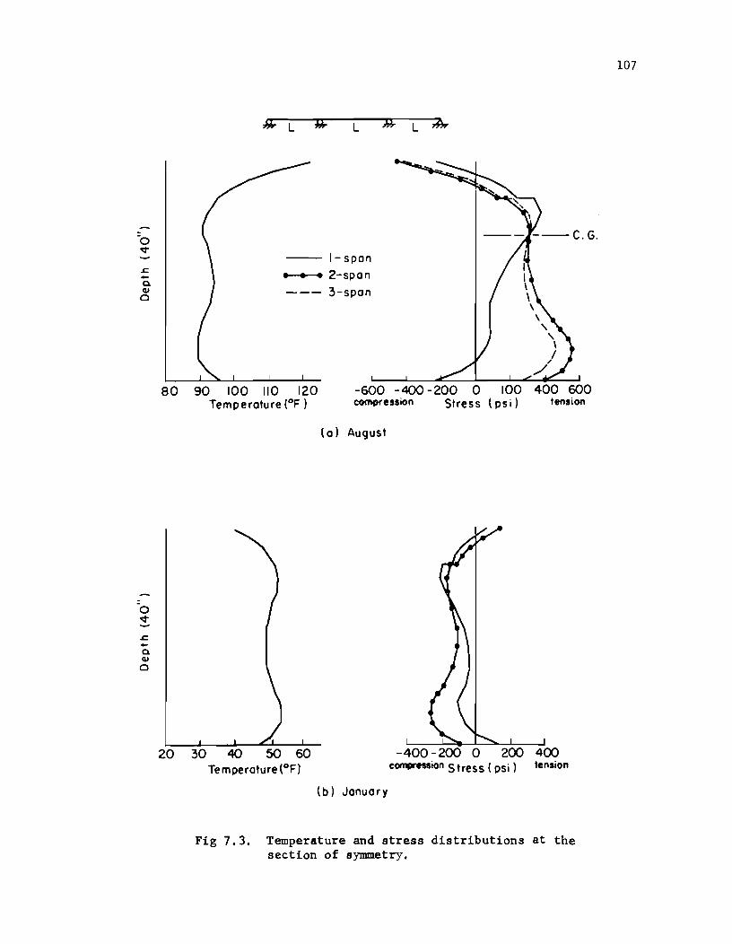
~ -c. C1I o
o v
c. C1I o
L
-- I-span
• • • 2-span
--- 3-span
80 90 100 110 120 Temperature (OF)
-600 - 400 - 200 0 100 400 600 compression Stress (psi) tension
(0) August
20 30 40 50 60 - 400 - 200 0 200 400 Temperature (OF) compression Stress (psi) tension
(b) January
Fig 7.3. Temperature and stress distributions at the section of symmetry.
107
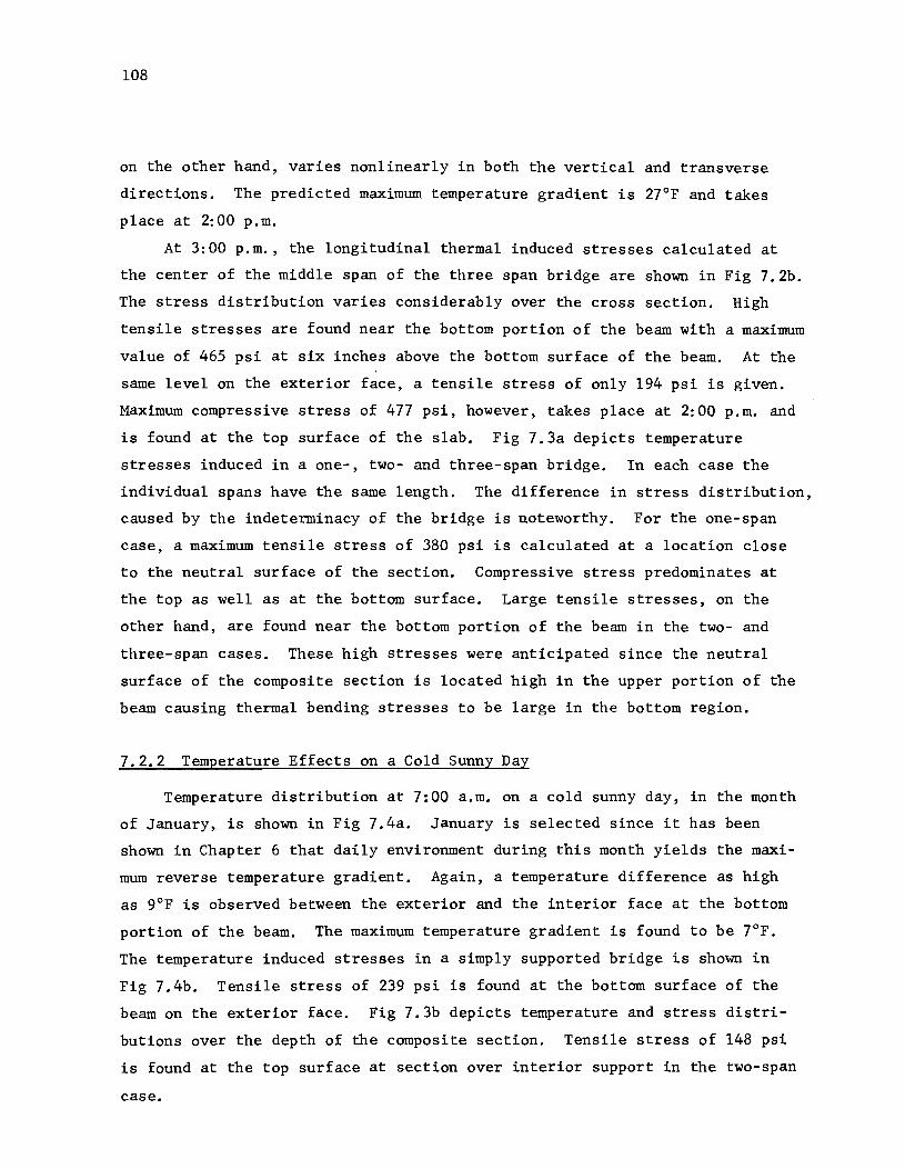
108
on the other hand, varies nonlinearly in both the vertical and transverse
directions. The predicted maximum temperature gradient is 27°F and takes
place at 2:00 p.m.
At 3:00 p.m., the longitudinal thermal induced stresses calculated at
the center of the middle span of the three span bridge are shown in Fig 7.2b.
The stress distribution varies considerably over the cross section. High
tensile stresses are found near the bottom portion of the beam with a maximum
value of 465 psi at six inches above the bottom surface of the beam. At the
same level on the exterior face, a tensile stress of only 194 psi is given.
Maximum compressive stress of 477 psi, however, takes place at 2:00 p.m. and
is found at the top surface of the slab. Fig 7.3a depicts temperature
stresses induced in a one-, two- and three-span bridge. In each case the
individual spans have the same length. The difference in stress distribution,
caused by the indeterminacy of the bridge is noteworthy. For the one-span
case, a maximum tensile stress of 380 psi is calculated at a location close
to the neutral surface of the section. Compressive stress predominates at
the top as well as at the bottom surface. Large tensile stresses, on the
other hand, are found near the bottom portion of the beam in the two- and
three-span cases. These high stresses were anticipated since the neutral
surface of the composite section is located high in the upper portion of the
beam causing thermal bending stresses to be large in the bottom region.
7.2.2 Temperature Effects on a Cold Sunny Day
Temperature distribution at 7:00 a.m. on a cold sunny day, in the month
of January, is shown in Fig 7.4a. January is selected since it has been
shown in Chapter 6 that daily environment during this month yields the maxi
mum reverse temperature gradient. Again, a temperature difference as high
as 9°F is observed between the exterior and the interior face at the bottom
portion of the beam. The maximum temperature gradient is found to be 7°F.
The temperature induced stresses in a simply supported bridge is shown in
Fig 7.4b. Tensile stress of 239 psi is found at the bottom surface of the
beam on the exterior face. Fig 7.3b depicts temperature and stress distri
butions over the depth of the composite section. Tensile stress of 148 psi
is found at the top surface at section over interior support in the two-span
case.
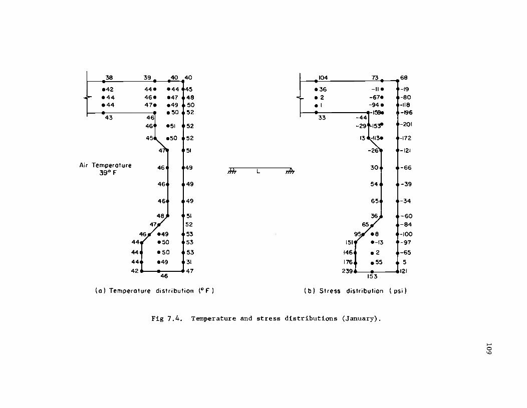
38 39 40 40 104 73_
.42 44. ·44 45 .36 -II.
.44 46. .47 48 "I"'" .2 -67.
.44 47. .49 50 .1 -94. .50 52 -158e
43 41 33 -44 46 ·51 52 -29 ~15~
45 .50 52 13 -113.
4 51 -26
Air Temperature 46 49
3°I 39° F IHT L n9r
46 49 54
46 49 65
51 52
53 44 .50 53 151
44 .50 53 146 .2
44 .49 31 176 .55 42 47 239
46 153
(a) Temperature distribution (0 F) (b) Stress distribution
Fig 7.4. Temperature and stress distributions (January).
68
-19 -80 -118 -196
-201
-172
-121
r" -39
-34
-60 -84
-100 -97
-65
5 121
( psi)
I-' o ~

110
7.2.3 General Remarks
It has been shown that temperature distribution through the depth of a
prestressed composite bridge subjected to daily environmental conditions is
nonlinear, and that it cannot be represented by a parabolic distribution as
was assumed by some pioneer researchers. This can be seen from Fig 7.3b
which indicates that distributions of temperature stresses, in general,
follow the shape of the temperature. Hence, an arbitrary temperature dis
tribution should not be used in computing the stresses. For the weather
conditions considered, the maximum tensile stress in the three span bridge
is 465 psi. This stress is approximately 80 percent of the cracking stress,
7.5 .~ where fl is the compressive strength of concrete at 28 days, ~~c c
given by the AASHO Specifications, section 1.6.7B. Of more importance is
the fact that this stress is additive to the design stresses caused by com
binations of dead load and live loads. For winter conditions, the stresses
show a sign change and have a magnitude of approximately 40 to 50 percent
of the summer values.
With regard to longitudinal movements, it is found that the range of
the rise and fall of bridge temperature from an assumed temperature, 60°F,
at the time of erection are 45°F. For comparison, the AASHO Specifications
recommend temperature rise and fall to be 30°F and 40°F respectively, section
1.2.15. Studies have also shown that vertical deflections are generally
small. However, the development of theoretical large interface shear force
and moment should be noted. These interface forces are induced by the
temperature difference between the concrete slab and steel beam. Effects of
these forces at the bridge interface will be discussed in section 7.4.
7.3 Composite Steel Bridge
This type of highway bridge has gained popularity due to its relatively
low cost, increased stiffness and increased overload capacity. The thermal
behavior of this bridge type has been a major concern to many research
engineers for years. Actual bridge temperature measurements were carried
out over a two year period by Zuk (58). Extensive field data has been
recorded and plots of daily temperature distribution over the depth presented
for both cold and warm sunny days. Results obtained from that work will be
used as spot checks in these theoretical studies.

111
Figure 7.5 depicts the idealization of a typical interior composite steel
beam. A total number of 46 rectangular elements with 71 nodal points were
used. The compressive strength of the concrete slab was assumed to be 3000
psi. Its average thermal properties are listed in Table 6.1. The modulus of
elasticity of the steel girder was taken to be 29 X 106 psi with a density of
490 1b/ft3 • The average thermal properties of structural steel are
coefficient of thermal expansion
thermal conductivity
specific heat
6.5X10- 6
26.6
0.11
7.3.1 Temperature Effects on a Warm Sunny Day
in/inrF
btu /ft /hr rF btu/1brF
Figure 7.6a shows predicted surface temperature distributions on a
warm sunny day in August. It is found that the maximum temperature diffe
rential through the depth of the bridge occurs at 2:00 p.m. and is 22°F.
In addition, the top surface temperature is about 21°F warmer than the
surrounding air temperature. Reference 58 reported this value to be 20°F to
30°F depending on the color of the concrete surface. The bottom flange
temperature is very close to the air temperature. This is due to the steel's
high conductivity. It is observed that in the late afternoon and during the
night, the bottom flange temperature is warmer than the air temperature.
This same phenomenon was also experimentally observed by Zuk (58).
Although a maximum temperature gradient occurs at 2:00 p.m., the maxi
mum tensile stress in the steel beam is found to take place a few hours
later. Consequently, it is the shape of the temperature distribution over
the cross section and not necessarily the highest thermal differential
between the top and bottom surface that induces the highest internal thermal
stress. Temperature distribution at 6:00 p.m. is shown in Fig 7.6b. As is
anticipated, bottom slab temperature affects the temperature at the top of
the steel beam. Temperature distribution in the concrete slab is nonlinear,
while a uniform gradient is found over a large portion of the steel beam.
Stress distributions at the section of symmetry in a one-, two- and three
span bridge are also presented in Fig 7.6b. For the three-span case, maximum
induced tensile stress in the beam is about 1000 psi. Maximum compressive

112
10 19
28 37
40 6.75" = 27"
2 3 4 (I) (2) (9 @ 0 0
38 39 40
," ," "+' " "1" "I" "I" =< 9 0.1875
1" --.l
41 46 47 ----r 0.3"
3
50
52
54
55. 625"
56
58
60
62
@- 1.125"
64 65 66 ~ 66 1
(44) 67 7(J 71 f L .1
8"
Fig 7.5. Typical interior girder idealization of a composite steel bridge.
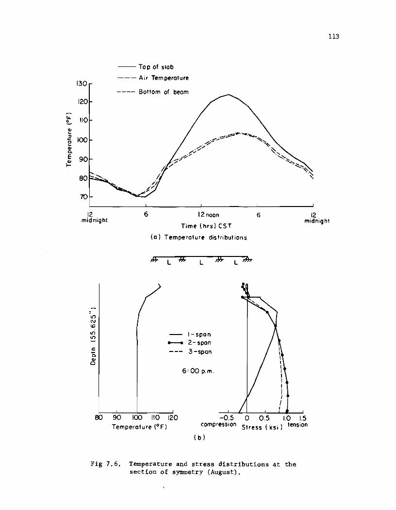
~ 0
CI.I ... ~ -0 ... CI.I Q.
E CI.I I-
130
120
110
100
90
80
70
12 midnight
-If)
N U)
If) If)
-- Top of slob
.-.-.- Air Temperature
---- Bottom of beam
6 12 noon
Time (hrs) CST
(0) Temperature distributions
L L
I-span .-- 2-span
3-span
6: 00 p.m.
L~
6
113
12 midnight
90 100 110 120 -0.5 0 0.5 1.0 1.5 Temperature (OF) compression Stress (ksi) tension
( b )
Fig 7.6. Temperature and stress distributions at the section of symmetry (August).
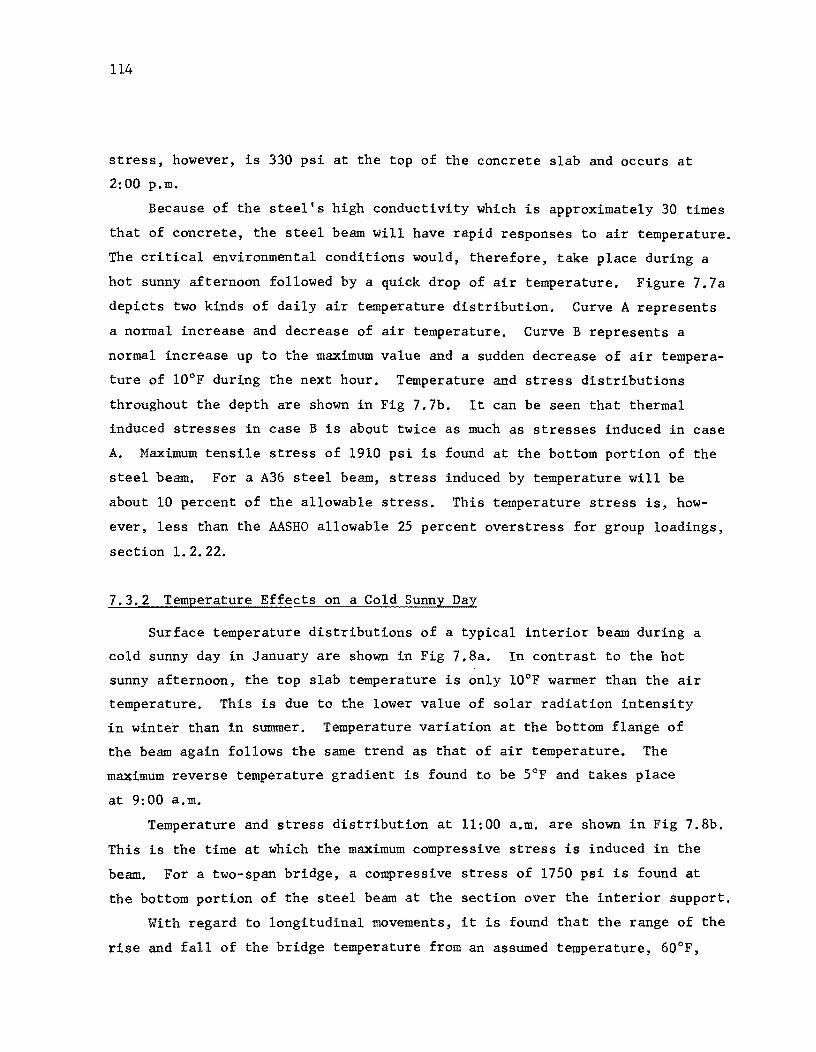
114
stress, however, is 330 psi at the top of the concrete slab and occurs at
2:00 p.m.
Because of the steel's high,conductivity which is approximately 30 times
that of concrete, the steel beam will have rapid responses to air temperature.
The critical environmental conditions would, therefore, take place during a
hot sunny afternoon followed by a quick drop of air temperature. Figure 7.7a
depicts two kinds of daily air temperature distribution. Curve A represents
a normal increase and decrease of air temperature. Curve B represents a
normal increase up to the maximum value and a sudden decrease of air tempera
ture of 10°F during the next hour. Temperature and stress distributions
throughout the depth are shown in Fig 7.7b. It can be seen that thermal
induced stresses in case B is about twice as much as stresses induced in case
A. Maximum tensile stress of 1910 psi is found at the bottom portion of the
steel beam. For a A36 steel beam, stress induced by temperature will be
about 10 percent of the allowable stress. This temperature stress is, how
ever, less than the AASHO allowable 25 percent overstress for group loadings,
section 1. 2. 22.
7.3.2 Temperature Effects on a Cold Sunny Day
Surface temperature distributions of a typical interior beam during a
cold sunny day in January are shown in Fig 7.8a. In contrast to the hot
sunny afternoon, the top slab temperature is only 10°F warmer than the air
temperature. This is due to the lower value of solar radiation intensity
in winter than in summer. Temperature variation at the bottom flange of
the beam again follows the same trend as that of air temperature. The
maximum reverse temperature gradient is found to be 5°F and takes place
at 9:00 a.m.
Temperature and stress distribution at 11:00 a.m. are shown in Fig 7.8b.
This is the time at which the maximum compressive stress is induced in the
beam. For a two-span bridge, a compressive stress of 1750 psi is found at
the bottom portion of the steel beam at the section over the interior support.
With regard to longitudinal movements, it is found that the range of the
rise and fall of the bridge temperature from an assumed temperature, 60°F,

1.1.. 0 .....-~ :::I -0 ... III Q.
E {!!.
110
100
90
80
70
12 6
- A (Normal)
--- B (Ex1reme)
\ \ , ,
'" ----
6
-.... .....
midnight 12noon
Time (CST) 12
midnight
.c -Q. III o
(a ) Air temperature conditions
/ / I I I I I I I I I I I I I \ \ ,
I'
.... ., .. -"
6:00p.m.
80 90 100 110 120 -.5 o Temperature (OF) compress ion
(b)
.... --
.5
---... , , , \ \ \ \ \ \ \ \ ,
I I
I I
1.5 2.0 Stress (ksi) tension
Fig 7.7. Temperature and stress sistributions at the section of symmetry (August).
115

116
90 -- Top of slab
-'-'- Air Temperature
80 ---- Bottom of beam
70
60
50
40
\
30~----~--------~-----------L--------~ 12
midnight
-a. CIJ Cl
6 12 noon
Time (CST)
(a) Temperature distributions
-- 1- span
- 2-span
II:OOa.m.
6 12 midnight
40 50 60 70 80 Temperature (OF)
-2.0 -1.5 -1.0 -0.5 0 0.5 compression St r e ss ( ksi ) tension
( b )
Fig 7.8. Temperature and stress distributions at the section of symmetry (January).
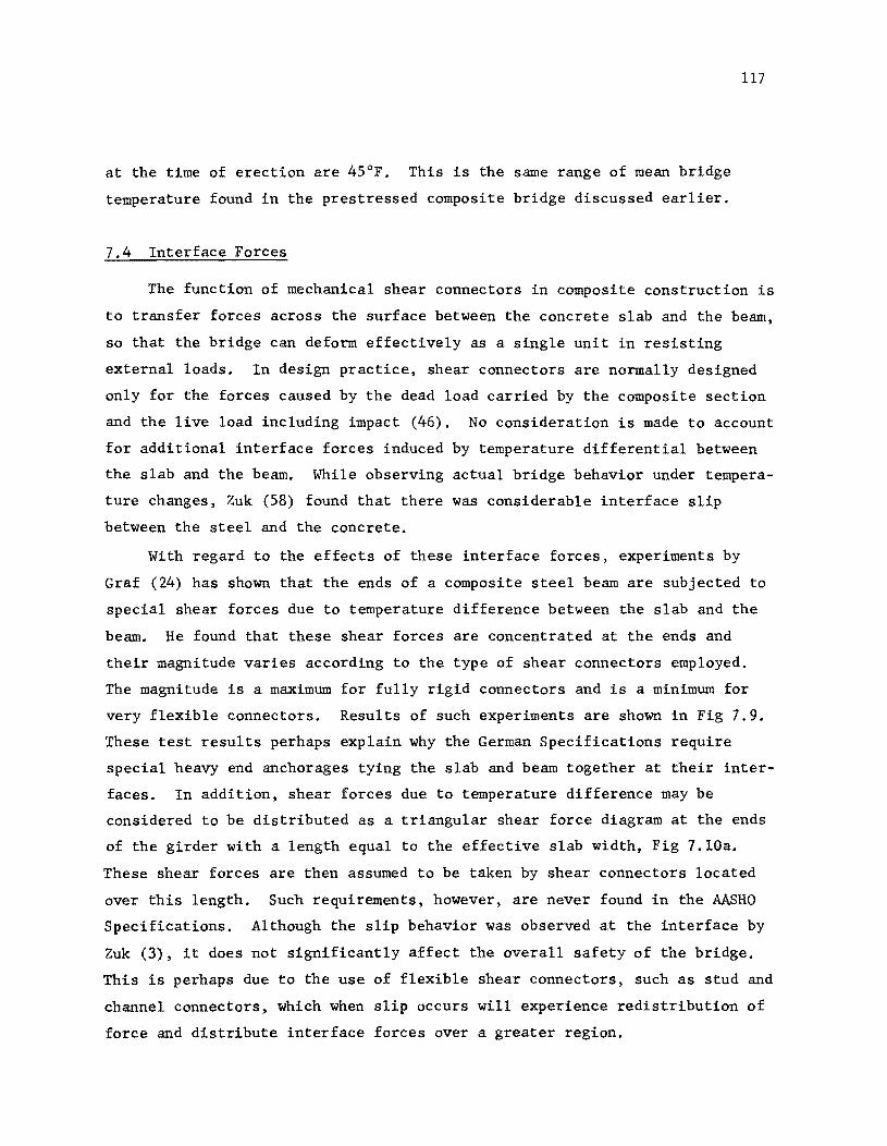
at the time of erection are 45°F. This is the same range of mean bridge
temperature found in the prestressed composite bridge discussed earlier.
7.4 Interface Forces
117
The function of mechanical shear connectors in composite construction is
to transfer forces across the surface between the concrete slab and the beam,
so that the bridge can deform effectively as a single unit in resisting
external loads. In design practice, shear connectors are normally designed
only for the forces caused by the dead load carried by the composite section
and the live load including impact (46). No consideration is made to account
for additional interface forces induced by temperature differential between
the slab and the beam. While observing actual bridge behavior under tempera
ture changes, Zuk (58) found that there was considerable interface slip
between the steel and the concrete.
With regard to the effects of these interface forces, experiments by
Graf (24) has shown that the ends of a composite steel beam are subjected to
special shear forces due to temperature difference between the slab and the
beam. He found that these shear forces are concentrated at the ends and
their magnitude varies according to the type of shear connectors employed.
The magnitude is a maximum for fully rigid connectors and is a minimum for
very flexible connectors. Results of such experiments are shown in Fig 7.9.
These test results perhaps explain why the German Specifications require
special heavy end anchorages tying the slab and beam together at their inter
faces. In addition, shear forces due to temperature difference may be
considered to be distributed as a triangular shear force diagram at the ends
of the girder with a length equal to the effective slab width, Fig 7.l0a.
These shear forces are then assumed to be taken by shear connectors located
over this length. Such requirements, however, are never found in the AASHO
Specifications. Although the slip behavior was observed at the interface by
Zuk (3), it does not significantly affect the overall safety of the bridge.
This is perhaps due to the use of flexible shear connectors, such as stud and
channel connectors, which when slip occurs will experience redistribution of
force and distribute interface forces over a greater region.
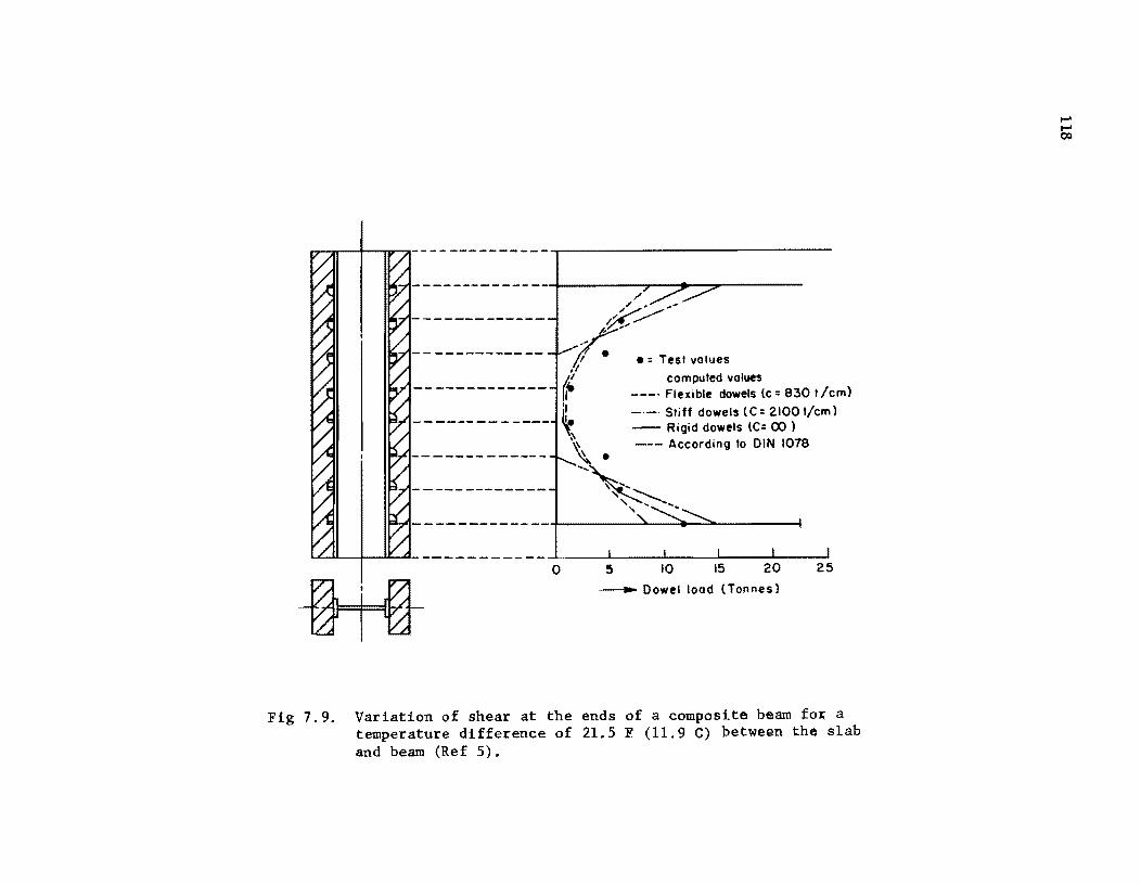
II 2. 10 A--------------.,----------------------------- J >... ........
/' ", ,'" "",'
"y..............~.- ....
/.' • = Test values ;1 ~ computed values If ---. Flexible dowels (c = 830 t /cm) iL _._. Stiff dowels (C: 2100 I/cm) ~ -- Rigid dowels (C= 00 )
,
-- According to DIN 1078 " .
~"
"\ " ",,~, " - ,
------------ " ...... :"'>.
I / " '" 4 ____________ ....L. ___ ..l-___ L--__ --L ___ --L. __ ---..l
o 5 10 15 20 25 ______ Dowel load (Tonnes)
Fig 7.9. Variation of shear at the ends of a composite beam fOH a temperature difference of 21.5 F (11.9 C) between the slab and beam (Ref 5).
t-' t-' ()Q
slab end
t
Total shear force (F)
effective slab width ( bf )
a) Triangular shear force diagram in accordance with the German code.
:.-
~. t "'-Sh,O' fo", (T)
TA Vertical anchorage
b) Temperature forces near slab end.
,
Fig 7.10. Interface forces near the slab end caused by a temperature differential.
119
UO
Since interface forces result from the strain compatibility requirements,
their magnitudes are, therefore, independent of the presence of interior
supports. Shear force is then computed by integrating temperature stresses
over the slab cross section in the single span case. According to the
author's analysis, the resultant shear force in the prestressed composite
bridge, Fig 7.1, is found to be 22400 lb. If no interface slip is allowed,
this force will be transmitted by shear across the interface near the ends.
Following the German code, this force will require additional shear con
nectors of approximately 50 percent of that required by the design load over
the length of the effective width of the slab. This transfer, of course,
results in a moment which is computed to be 185000 1b in. This moment is
transferred by creating a vertical holding down force with a balancing
compressive force across the interface, ~ig 7.10b. Therefore, vertical end
anchorages are required to prevent curling of the interface. For the com
posite steel bridge, Fig 7.5, the interface shear and moment are found to be
6000 1b and 96000 1b in., respectively. From the German code, this force
will again require additional shear connectors of approximately 50 percent
of that required by the dead and live loads at the ends of the steel beam.
7.5 Pedestrian Overpass (Narrow Structure)
A pedestrian overpass located in Austin, Texas was field tested on
14 March 1975. This test was performed as part of this research project and
will be further discussed in the next project report. The bridge is a two
span composite prestressed structure with perpendicular supports. Its
transverse section including parapets, slab deck and girders are shown in
Fig 7.11b. Although the structure was designed as a pedestrian overpass,
the slab thickness, the size of the girder and the spacing between the
center-to-center of the two girders are commonly found in highway bridges of
this type. Consequently, the bridge is considered as a narrow structure in
which the thermal response is of interest for study.
Due to the fact that this structure has only two I-beams and is oriented
at an angle to the sun's path, the temperature distributions will be complex
due to side heating of the girders and shading of the slab by the parapets.
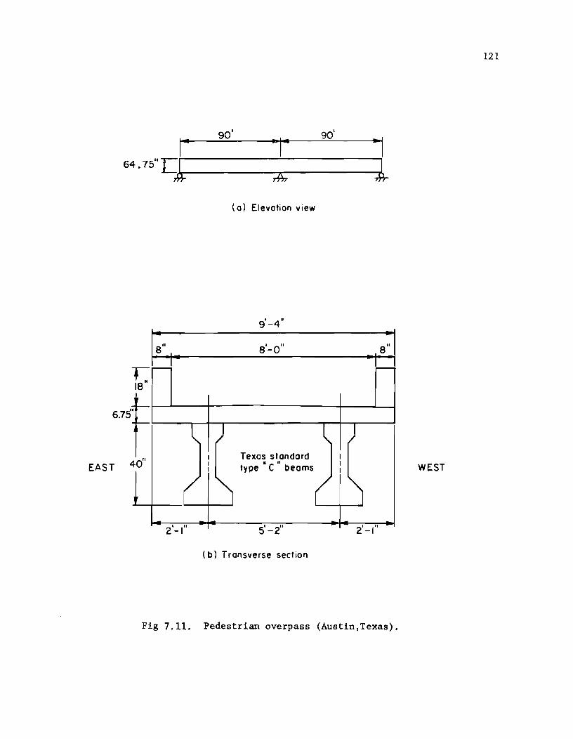
121
I" 90' -,- 90'
~I
64.75"L"I A 1
(0) Elevation view
9'-4"
S'-o"
.--:-IS
6.75"
Texas standard . " type C beams EAST 40" WEST
5'-2"
(b) Transverse section
Fig 7.11. Pedestrian overpass (Austin,Texas).
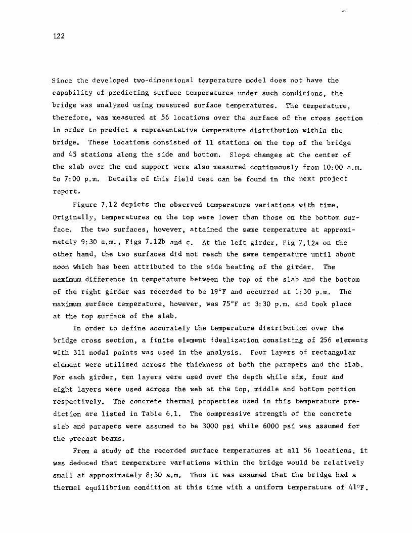
122
Since the developed two-dimensional temperature model does not have the
capability of predicting surface temperatures under such conditions, the
bridge was analyzed using measured surface temperatures. The temperature,
therefore, was measured at 56 locations over the surface of the cross section
in order to predict a representative temperature distribution within the
bridge. These locations consisted of 11 stations on the top of the bridge
and 45 stations along the side and bottom. Slope changes at the center of
the slab over the end support were also measured continuously from 10:00 a.m.
to 7:00 p.m. Details of this field test can be found in the next project
report.
Figure 7.12 depicts the observed temperature variations with time.
Originally, temperatures on the top were lower than those on the bottom sur
face. The two surfaces, however, attained the same temperature at approxi
mately 9:30 a.m., Figs 7.l2b and c. At the left girder, Fig 7.12a on the
other hand, the two surfaces did not reach the same temperature until about
noon which has been attributed to the side heating of the girder. The
maximum difference in temperature between the top of the slab and the bottom
of the right girder was recorded to be 19°F and occurred at 1:30 p.m. The
maximum surface temperature, however, was 75°F at 3:30 p.m. and took place
at the top surface of the slab.
In order to define accurately the temperature distribution over the
bridge cross section, a finite element idealization consisting of 256 elements
with 311 nodal points was used in the analysis. Four layers of rectangular
element were utilized across the thickness of both the parapets and the slab.
For each girder, ten layers were used over the depth while six, four and
eight layers were used across the web at the top, middle and bottom portion
respectively. The concrete thermal properties used in this temperature pre
diction are listed in Table 6.1. The compressive strength of the concrete
slab and parapets were assumed to be 3000 psi while 6000 psi was assumed for
the precast beams.
From a study of the recorded surface temperatures at all 56 locations, it
was deduced that temperature variations within the bridge would be relatively
small at approximately 8:30 a.m. Thus it was assumed that the bridge had a
thermal equilibrium condition at this time with a uniform temperature of 41°F.
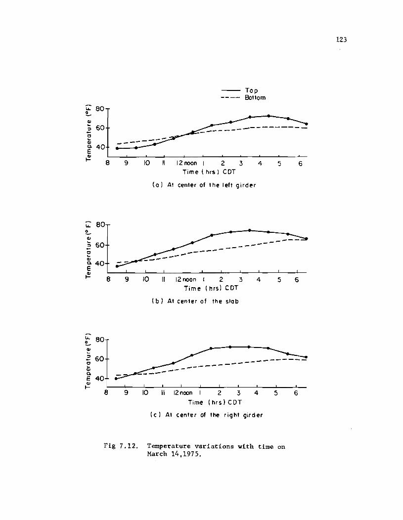
I.t.. ~
80
QI ... 60 ~ -0 ... QI a. 40 E QI
to-
I.t.. 80
QI
~ 60 o ... QI a. 40 E QI
8
to- e
I.t.. 80 ~ QI ... ~ 60 -0 ... QI a. E 40 QI
to-e
--9 10
9 10
9 10
Top Bottom
-------------
II 12 noon 1 2 3 4 5 6 Time ( hrs) COT
(0) At center of the left girder
----------... -----
" 12 noon I 2 3 4 5 6 Time (hrs) COT
(b) At center of the slob
------------.-------
II 12 noon I 2 3 4 5 6 Time (hrs)CDT
(c) At center of the right girder
Fig 7.12. Temperature variations with time on March 14,1975.
123
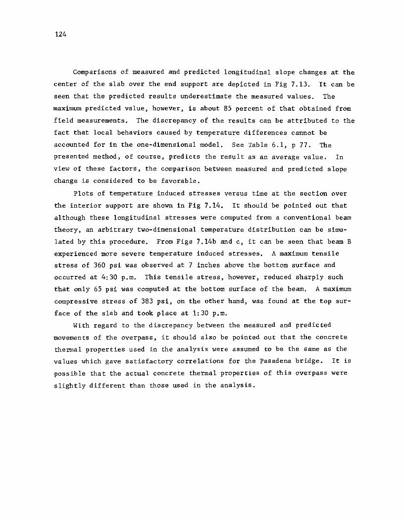
124
Comparisons of measured and predicted longitudinal slope changes at the
center of the slab over the end support are depicted in Fig 7.13. It can be
seen that the predicted results underestimate the measured values. The
maximum predicted value, however, is about 85 percent of that obtained from
field measurements. The discrepancy of the results can be attributed to the
fact that local behaviors caused by temperature differences cannot be
accounted for in the one-dimensional model. See Table 6.1, p 77. The
presented method, of course, predicts the result as an average value. In
view of these factors, the comparison between measured and predicted slope
change is considered to be favorable.
Plots of temperature induced stresses versus time at the section over
the interior support are shown in Fig 7.14. It should be pointed out that
although these longitudinal stresses were computed from a conventional beam
theory, an arbitrary two-dimensional temperature distribution can be simu
lated by this procedure. From Figs 7.14b and c, it can be seen that beam B
experienced more severe temperature induced stresses. A maximum tensile
stress of 360 psi was observed at 7 inches above the bottom surface and
occurred at 4:30 p.m. This tensile stress, however, reduced sharply such
that only 65 psi was computed at the bottom surface of the beam. A maximum
compressive stress of 383 psi, on the other hand, was found at the top sur
face of the slab and took place at 1:30 p.m.
With regard to the discrepancy between the measured and predicted
movements of the overpass, it should also be pointed out that the concrete
thermal properties used in the analysis were assumed to be the same as the
values which gave satisfactory correlations for the Pasadena bridge. It is
possible that the actual concrete thermal properties of this overpass were
slightly different than those used in the analysis.
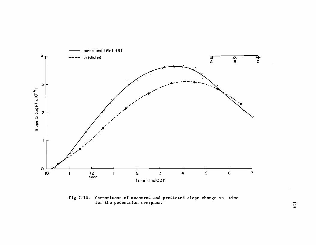
4
3
<t"
'0 )(
CLI C7' c 2 0 ..c U
CLI a. .2 (f)
I / 0
10
,. , ~ '"
y '"
II
mea sured (Ref. 49)
predicted
",'" '" " " " ,-
'" ,If ;' ,-
,-,-'" " ,
12 noon
'" "
}); ~ ~ A 8 C
.......... ---- ........ -........ -" """" ....... ,.
........ " ....
2
.......
3
Time (hrs)C DT
4 5 6 7
Fig 7.13, Comparisons of measured and predicted slope change vs, time for the pedestrian overpass, I-'
N V1

126
III III GI ...
(f')
III III GI ...
(f')
400 c 0
en c 200 ~
0 c 0 en
-200 en G> ... a. E 0 -400 u
400 c 0 en c !! 200
0 c 0
en en
-200 G> ... a. E 0 -400 u
EAST WEST
10
A
(a) Bridge section
Top ---- Bottom
B
Location of maximum stress
( ?" above the bottom)
2 4 5 11' ........ ,12 _------ 6 7 Time (hrs) COT
--- -'""::::'- .............. -_ .... ........ , /
.......... _- ,/' -......... .,....,. .............. --,
( b) Temperature stresses vs time (Beam A)
--- --------- - -------Time (hrs) COT
10 II 12 2:3 4 5 ~ 7 __ noon .-'
-.......... r - / .......... '" - ---............... ----~
(c) Temperature stresses vS time ( Beam B)
Fig 7.14. Longitudinal temperature induced stresses vs. time at the center section over the interior support.
CHAPTER 8. SUMMARY, CONCLUSIONS AND RECOMMENDATIONS
8.1 Sunnnary
The computational procedures for the prediction of the transient bridge
temperature distribution and the resulting structural response have been
developed. The purpose of which is to assess the significance of the ther
mal effects in three types of highway bridges. They are 1) a post-tensioned
concrete slab bridge, 2) a composite precast pretensioned bridge, and 3) a
composite steel bridge. Particular attention is given to the study of bridge
behaviors under the extreme environmental conditions that have existed in
Austin, Texas.
Numerical procedures as applied to the heat transfer analysis can
represent both the one-dimensional and two-dimensional heat flow. Boundary
conditions at the exterior surfaces of the bridge are those of solar radia
tion intensity, ambient air temperature and wind speed. The one-dimensional
heat equation is written in finite difference form and temperatures over the
bridge cross section are determined by an incremental process. The finite
element method, however, is used in determining the distribution of tempera
ture over the bridge cross section where the flow of heat varies two-dimen
sionally. The temperature distribution along the length of the bridge, on
the other hand, is assumed to be constant.
The structural response under temperature changes is assumed to be in
the elastic range. Structural stiffness is computed based on the uncracked
section. Temperature induced stresses and deformations are calculated based
on the one-dimensional beam theory. Hence, the method is limited to straight
bridges with supports perpendicular to the longitudinal direction of the
bridge. Temperature effects in both simple span and continuous span bridges
were studied.
All of these computations are included in a computer program to form a
complete system for predicting temperature behaviors of highway bridges
exposed to atmospheric conditions. Documentations of this computer program,
TSAP (Temperature and Stress Analysis Program), will be in a later project report.
127
128
The input data required to use the program is easy to obtain. Environmental
data can be obtained from regular Weather Bureau Reports and material thermal
properties can be obtained from handbooks or Table 3.3.
8.2 Conclusions
The study demonstrates the feasibility and validity of analytically
predicting the structural response of a bridge structure subjected to daily
atmospheric variations. The method presented has been shown to be quite
general in that it can be used to treat various conditions of the environ
ment, types of highway bridge cross section as well as the indeterminacy of
the structure. Although the study focused on the climatic conditions that
have existed in Austin, Texas, other locations can also be studied if the
relevant weather conditions are input.
It is found that the important weather parameters influencing the
bridge temperature distributions are radiation, ambient air temperature and
wind speed. Incoming solar radiation is the primary source that increases
the top surface temperature during the day. Outgoing radiation, on the
other hand, results in decreasing bridge temperature during the night. The
important material thermal properties are the absorptivity, emissivity and
thermal conductivity. Shape, size and thickness of the structure also
affects the temperature variations over the bridge cross section.
The extreme environmental conditions have been found to take place on a
clear night followed by a clear day with a large range of air temperature.
In general, on a clear sunny day, the maximum incoming solar radiation
intensity occurs at about noon, the peak ambient air temperature occurs at
4:00 p.m., and yet the top surface temperature is found to be maximum at
2:00 p.m. The maximum temperature gradient over the bridge depth also
occurs at this time. On a clear night, the minimum surface temperature and
the maximum reverse gradient are normally found to take place one hour
before sunrise. The presence of wind at these times will reduce the maxi
mun values of the temperature gradient.
Thermal deflections are found to be small. The range of the longi
tudinal movement of the studied bridges is found to be somewhat greater
than the value suggested by the AASHO Specifications, section 1.2.15.

129
Temperature induced stresses appear to be significant. The magnitude of
these stresses is found to be a function of the temperature distribution
over the depth of the bridge cross section whether the bridge i~ statically
determinatec'or indeterminate. It is also a function of the modulus of
elasticity and the coefficient of thermal expansion and contraction of the
material. For the weather conditions considered, the temperature induced
tensile stresses in a post-tensioned concrete slab bridge and a composite
precast pretensioned bridge are found to be in the order of 60 and 80 per
cent respectively of the cracking stress of concrete recommended by the
AASHO, section 1.6.7B. On the other hand, stresses induced by temperature
are approximately 10 percent of the design dead and live load stresses in a
composite steel bridge. However, this magnitude of stress is less than
AASHO's allowable 25 percent overstress for group loadings, section 1.2.22.
Therefore, in the composite steel bridge, the temperature induced stresses
are generally within tolerable design limits.
In general, highway bridges will be subjected to cyclic temperature
induced stress at 30 cycles per month (365 cycles per year), and the fre
quency of one cycle in 24 hours. Furthermore, the fluctuations of stresses
are not at their maximum values. Therefore, it is believed that this cyclic
character should not be compared with behaviors observed from a fatigue test
in which several hundred cycles per minute are normally applied.
It is also found that the interface shear force caused by the tempera
ture difference between the slab and the beam is of considerable magnitude.
Consequently, temperature effects may cause slip to take place earlier.
8.3 Recommendations
The method presented has made it possible to study computationally the
temperature effects in highway bridges subjected to various conditions of
the environment. With this capability it is suggested that further investi
gation be made on different types of highway bridge cross sections, for
example, a box girder bridge. Weather conditions at different locations and
different latitudes can also be included in the study.
Although it would be a major undertaking, it is a possibility to incor
porate the effect of the sun's rays which fall along the side of the bridge
in the computer program.

DO
Another topic of practical interest is the use of the computer program
TSAP, developed in this work to serve as a design tool to determine the
maximum temperature induced stresses in the bridge under investigation.
After these stresses have been defined, they can then be superimposed with
the dead load and live load stresses in order to obtain the final design
stresses.

APPENDIX A
COEFFICIENTS OF MATRICES FOR
A PLANE TRIANGULAR ELEMENT


APPENDIX A. COEFFICIENTS OF MATRICES FOR A PLANE TRIANGULAR ELEMENT
A typical triangular element is shown in Fig A.l. Temperature dis
tribution within the element is assumed to be linear, i.e.,
U(x,y) t (x,y) E (A. 1)
and U(x,y) dJ (x,y) 8 (A. 2) '"
where £ (x,y) = [ 1 x y] (A.3)
[~1 ~~ ct 0'2 and ~ 13 2 '"
0'3 133
(A.4)
Equation A.l is evaluated at three vertices of the triangle and the
three equations are solved simultaneously, finally we have
• ~
Au ~ Au (A.S) ~ '" ~
where A 1 [b/'- bk bk -b. (A.6)
~ A J
~ - a j -~ a. J
[1 ui , and • .
A a}k - ~bj u = u. u u. (A. 7) J .J
~ ~
133

134
y
0" j
~------------------------------------~x
Fig A.l. A typical triangular element.

135
Rewritten equations A.l and A.2
U(x,y) = ~ (x,y) ~:: Nu ~ '"
(A.8)
• . U(x, y) = cb (x,y) Au Nu
~ ~~ ~ '" (A. 9)
'1 U(x,y) Y,2(x,y) ~:: Du ~'"
(A. 10)
where D [!] [ 1 x y] A ~ ~
D 1 [bj - bk bk -bj or =
~ ). ~ -aj
a. -~
(A. 11)
For an isotropic triangular ele:nent with constant thickness, t , the
conductivity matrix is
e 2 +d 2 bke - ~d b.e+a.d
J J
B kt
bke - ~d 2 2
bj~ - aj~ ~ 2). bk +ak (A.12)
b.e+a.d bj~ - aj~ 2 2 b. +a.
J J J J
where d ~ - a j (A. 13)
and e = bj - bk (A.14)
For the heat capacity matrix, the lumped method is used instead of
Eq 4.26. The heat capacity is lumped at exterior nodes. Therefore,
the diagonal coefficients are, Fig A.l,

136
(A.15)
If both convection and radiation take place only on the i-j face with
the constant film coefficient, the matrix H is then ~
h t·· H .. H ..
C l.J = = 3 l.l. JJ
hct .. and Hij = l.J
6
(A.l6)
The vector h* is also given by
h* (A.17)
The heat vector q* is
q* [~] (A.18)

APPENDIX B
EFFECT OF PRESTRESSING STEEL ON END FORCES

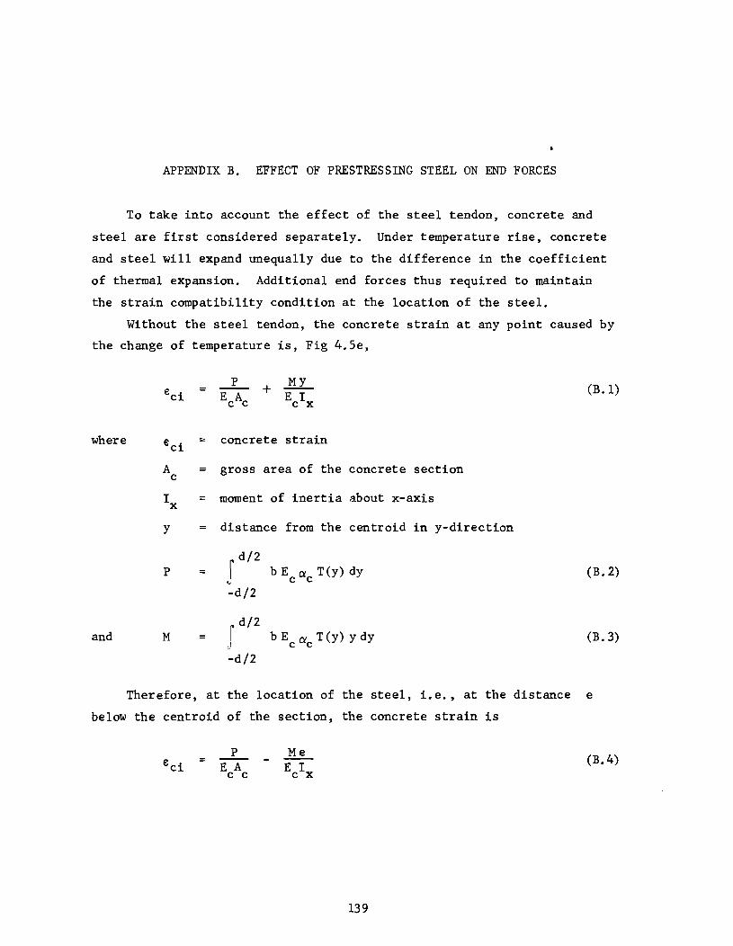
APPENDIX B. EFFECT OF PRESTRESSING STEEL ON END FORCES
To take into account the effect of the steel tendon, concrete and
steel are first considered separately. Under temperature rise, concrete
and steel will expand unequally due to the difference in the coefficient
of thermal expansion. Additional end forces thus required to maintain
the strain compatibility condition at the location of the steel.
Without the steel tendon, the concrete strain at any point caused by
the change of temperature is, Fig 4.5e,
P + ~ eci EcAc E I c x (B.1)
where €ci :, concrete strain
A gross area of the concrete section c
I = moment of inertia about x-axis x
y distance from the centroid in y-direction
P I d/2
bE ex T(y) dy "
c c (B.2)
-d/2
and M = r d/2
bE ex T(y) Y dy ~) c c (B.3)
-d/2
Therefore, at the location of the steel, i. e. , at the distance e
below the centroid of the section, the concrete strain is
P Me (B.4) eci E A E I c c c x
139

140
The strain of the steel, under free expansion, is
= (B.5)
Let F be the end force, compression in the steel and tension in s
the concrete, which acts at the location of the tendon. The final concrete
strain is, therefore,
where
and
= F
s eci + 'EA +
c c
F 2 J;.e
E I c x
Similarly, the final steel strain is
= est - E A s s
Since €c = €s ' from Eqs B.6 and B.7 we have
€si - €ci F
s (
1 1 _. e 2- ~ 'EA+'EA+EII
c C S S C x
Consequently, thermal induced stresses are given by
pI +
M/Y E ex T (y) O'c =
A I c c c x
pI = P+F s
M' = M - F e s
(B.6)
(B.7)
(B.8)
(B.9)
(B.lO)
(B.ll)
BIBLIOGRAPHY
1. Barber, E. S., "Calculation of Maximum Pavement Temperatures from Weather Reports," Highway Research Board Bulletin 168, pp. 1-8, 1957.
2. Becker, E. B., and Parr, C. H., "Application of the Finite Element Method to Heat Conduction in Solids," Technical Report S-117, U.S. Army Missile Command, Redstone Arsenal, Alabama, November 1968.
3. Berks, C. J., "New Mechanical Bridge Joint System," Civil Engineering, Vol. 68, No. 741, London, April 1968, pp. 439-440.
4. Berwanger, C., "Thermal Stresses in Composite Bridges," The Journal of the Institute of Structural Engineers, April 1974.
5. Billington, N. S., Thermal Properties of Buildings, Cleaver-HumecPress, LTD., 1952.
6. Boley, B. A., and Weiner, J. H., Theory of Thermal Stress, John Wiley & Sons, Inc., 1960.
7. Boresi, A. P., Elasticity in Engineering Mechanics, Prentice-Hall, Inc., Englewood Cliffs, New Jersey, 1965.
8. Brisbane, J. J., Heat Conduction and Stress Analysis of Anisotropic Bodies, Vol. 1, Rohm· and Haas Company, Redstone Research Laboratories, Huntsville, Alabama, October 1969.
9. Brisbane, J. J., Becker, E. B., and Parr, C. H., "The Application of the Finite Element Method to the Solution of Stress and Diffusion Problems of Continua," Journal of the Alabama Academy of Science, Vol. 39, No.2, April 1968.
10. Capps, M. W. R., "The Thermal Behavior of the Beachley Viaduct/Wye Bridge," RRL Report, LR 234, Road Research Laboratory, Ministry of Transport, London, England, 1968.
11. Carslaw, H. S., and Jaeger, J. C., Conduction of Heat in Solids, Oxford University Press,. 2nd Edition, "London., 1959.
12. Chapman, A. J., Heat Transfer, The Macmillan Company, 2nd Edition, 1960.
13. Climates of the States, Vol. II, Western Series, U.S. Department of Connnerce, 1974.
141
142
14. "Climatological Data," The U.S. Weather Bureau Reports, National Summary, Environmental Science Services Administration, Environmental Data Service.
15. Crandall, S. H., and Dahl, N. C., An Introduction to Mechanics of Solids, McGraw-Hill 1959.
16. Desai, C. S., and Abel, J. F., Introduction to the Finite Element Method, Van Nostrand Reinhold Company, 1972.
17. Ekberg, C. E., Jr., and Emanuel, J. H., "Current Design Practice for Bridge Bearing and Expansion Devices," Final Report, Project 547-9, Engineering Research Institute, Iowa State University, Ames, Iowa, August, 1967.
18. Emanuel, J. H., and Eckberg, C. E., Jr., "Problems of Bridge Supporting and Expansion Devices and an Experimental Comparison of the Dynamic Behavior of Rigid and Elastomeric Bearings," Special Report, Iowa State University, Iowa Engineering Experiment Station, September, 1965.
19. Emanuel, J. H., Best, J. L., Hulsey, J. L., Senne, J. H., and Thompson, L. E., "An Investigation of Design Criteria for Stresses Induced by Semi-Integral End Bents," Phase I-Feasibility Study, Civil Engineering Department, University of Missouri-Rolla, Rolla, Missouri, Study 72-1.
20. Emerson, M., "The Calculation of the Distribution of Temperature in Bridges," TRRL Report LR 561, Transport and Road Research Laboratory, Department of the Environment, Crowthorne, 1973.
21. Gaumer, G. R., "Stability of Three Finite Difference Methods of Solving for Transient Temperatures," Journal of American Rocket Society, Vol. 32, No. 10., 1962, pp. 1595-1596.
22. Gloyne, R. W., "The Diurnal Variation of Global Radiation on a Horizontal Surface - with Special Reference to Aberdeen," Meteorological Magazine 101, 1972, pp. 44-48.
23. Gortz, W., Agnew, F. S., and Palmer, M. F., "Bridge Deck Expansion Joints," Consulting Engineer, Vol. 31, No.5, London, May, 1967, pp. 76-78, 81.
24. Graf, 0., "Uber Versuche mit Verbundtragen," Der Bauingenieur, January, 1950, Heft 8.
25. Griffiths, E., and Davis, A. H., "Transmission of Heat by Radiation and Convection,tl Food Investigation Board, Special Report 9, 1922.
26. Gurtin, M. E., "Variational Principles for Linear Initial Value Problems," Quarterly Applied Mathematics, Vol. 23, 1964.
27. "Heating, Ventilating, Air Conditioning Guide," American Society of Heating and Air Conditioning Engineers, Vol. 37, 1959, p. 52.
28. Hendry, A. W., and Page, J. K., "Thermal Movements and Stresses in Concrete Slabs in Relation to Tropical Conditions," Rilem Symposium II 1960, International Symposium of Concrete and Reinforced Concrete in Hot Countries.
143
29. Hudson, F. M., "Investigation of a Full-Size Continuous Concrete Highway Bridge, Parts I and II," Final Report, HPR Report No. 24, Alabama Highway Research, Alabama Highway Department, June, 1967.
30. Hudson, F. M., "Simulation of Settlement of Supports of a Full Scale Continuous Concrete Bridge," Final Report, HPR Report No. 49, Alabama Highway Research, Alabama Highway Department, June, 1970.
31. Johns, D. J., Thermal Stress Analyses, Pergamon Press, 1965.
32. Johnson, C. P., and Matlock, H., "Temperature Induced Stresses in Highway Bridges by Finite Element Analysis and Field Tests," Proposal submitted for Research Project 3-5-74-23, Center for Highway Research, The University of Texas at Austin, May, 1970.
33. Kreith, F., Principles of Heat Transfers, International Text Book Company, 2nd Edition, 1965.
34. Krishanamurthy, N., "Temperature Effects on Continuous Reinforced Concrete Bridge," HPR Report No. 58, Research Project 930-047, State of Alabama Highway Department, July, 1971.
35. Liu, Y. N., Zuk, W., "Thennoelastic Effects in Prestressed Flexural Members," Journal of Prestressed Concrete Institute, Vol. 8, No.3, June, 1963, pp. 64-85.
36. Maher, D. R. H., "The Effects of Differential Temperature on Continuous Pres tres sed Concrete Bridges," Ci viI Engineering Transactions, Institute of Engineering, Vol. CE12, No.1, paper 2793, April, 1970, pp. 29-32.
37. Matlock, H., Panak, J. J., Vora, M. R., and Chan, J. H. C., "Field Investigation of a Skewed, Post-stressed Continuous Slab Structure Structure," Interim Study Report, Center for Highway Research, Research Project 3-5-63-56, The University of Texas at Austin, Texas, May 1970.
144
38. Meenan, A. R., "Parking Garages for New Orleans Superdome," Journal of Prestressed Concrete Institute, Vol. 19, No.2, March-April, 1974, pp. 98-111.
39. Monteith, J. L., "Light Distribution and Photosynthesis in Field Corps," Ann. Bot., London 29, 1965, pp. 17-37.
40. Narouka, M., Hirai, 1., and Yamaguti, T., "Measurement of the Temperature of the Interior of the Reinforced Concrete Slab of the Shigita Bridge and Presumption of Thermal Stress," Proceedings, Symposium of the Stress Measurements for Bridge and Structures, Japanese Society for the Promotion of Science, Tokyo, Japan, 1957, pp. 106-115.
41. "Standard Specifications for Highway Bridges," Associati.on of State Highway Officials, Washington, D.C., 1973.
42. Strock, C., and Koral, R. L., Handbook of Air Conditioning Heating and Ventilating, Industrial Press, Inc., 2nd Edition, 1965.
43. SWinbank, W. C., "Long-Wave Radiation from Clear Skies," Quarterly Journal of Royal Metoro1ogica1 Society, Vol. 89., 1963, pp. 339-348.
44. Timoshenko, S. P., Theory of Elasticity, McGraw-Hill, 3rd Edition, 1970, pp. 439-441.
45. Van Wyk, H. F., "Aspects of Thermal Stresses in Reinforced Concrete Structures Subjected to Differential Temperature Change," Ri1em Symposium, International Symposium of Concrete and Reinforced Concrete in Hot Countries, 1960.
46. Viest, I. M., Fountain, R. S., and Singleton, R. C., Composite Construction in Steel and Concrete, McGraw-Hill, 1958.
47. Visser, W., "A Finite Element Method for the Determination of Non-S tationary Temperature Distribution and Thermal Deformations," Proceedings, Second Conference on Matrix Methods in Structural Mechanics, Wright-Patterson Air Force Base, Ohio, November, 1966.
48. Wah, T., and Kirksey, R. E., "Thermal Characteristics of Highway Bridges," Final Report, No. HR 12-4, Southwest Research Institute, July, 1969.
49. Will, Kenneth M., Johnson, C. Philip, and Matlock, Hudson, '~na1ytica1
and Experimental Investigation of the Thermal Response of Highway Bridges," Research Report No. 23-2, Center for Highway Research, The University of Texas at Austin, February 1977.
50. Willems, N., "Experimental Strain Analysis of Continuous Skew Slab Bridge Decks," CRES Project No. 2070, Final Report, University of Kansas, October, 1973.
145
51. Williamson, P. J., "The Estimation of Heat Outputs for Road Heating Installations," Road Research Laboratory, LR Report 77, Ministry of Transport, 1967.
52. Wilson, E. L., "The Determination of Temperatures within Mass Concrete Structures,1I Structural Engineering Laboratory Report 68-17, University of California, Berkeley, California, December, 1968.
53. Wilson, E. L., and Nickell, R. E., IIApplication of the Finite Element Method to Heat Conduction Analysis," Nuclear Engineering and Design, Vol. 4, 1966, pp. 276-286.
54. Yan, H. T., Composite Construction Steel and Concrete, Orient Longmans, 1965.
55. Zienkiewicz, O. C., The Finite Element Method in Engineering Science, McGraw-Hill, 1971.
56. Zienkiewicz, o. C., and Parekh, C. J., "Transient Field Problems -Two and Three Dimensional Analysis of Isoparametric Finite Elements," International Journal for Numerical Methods in Engineering, Vol. 2, Wiley-Interscience, London, 1970.
57. Zuk, W., "Thermal and Shrinkage Stresses in Composite Beams," Journal of American Concrete Institute, Vol. 58, No.3, September, 1961, pp. 327-340.
58. Zuk, W., "Thermal Behavior of Composite Bridges Insulates and Uninsu1ated," Highway Research Record, No. 76, 1965, pp. 231-253.
59. Zuk, W., "Simplified Design Check of Thermal Stresses in Composite Highway Bridges," Highway Research Record, No. 103, 1965, pp. 10-13.
60. Zuk, W., "End Movement Studies of Various Type Highway Bridges,1I Highway Research Record, No. 295, 1969.
Related Documents