Prediction of perceptual similarity based on time-domain models of auditory perception Citation for published version (APA): Osses Vecchi, A. A. (2018). Prediction of perceptual similarity based on time-domain models of auditory perception. [Phd Thesis 1 (Research TU/e / Graduation TU/e), Industrial Engineering and Innovation Sciences]. Technische Universiteit Eindhoven. Document status and date: Published: 19/09/2018 Document Version: Publisher’s PDF, also known as Version of Record (includes final page, issue and volume numbers) Please check the document version of this publication: • A submitted manuscript is the version of the article upon submission and before peer-review. There can be important differences between the submitted version and the official published version of record. People interested in the research are advised to contact the author for the final version of the publication, or visit the DOI to the publisher's website. • The final author version and the galley proof are versions of the publication after peer review. • The final published version features the final layout of the paper including the volume, issue and page numbers. Link to publication General rights Copyright and moral rights for the publications made accessible in the public portal are retained by the authors and/or other copyright owners and it is a condition of accessing publications that users recognise and abide by the legal requirements associated with these rights. • Users may download and print one copy of any publication from the public portal for the purpose of private study or research. • You may not further distribute the material or use it for any profit-making activity or commercial gain • You may freely distribute the URL identifying the publication in the public portal. If the publication is distributed under the terms of Article 25fa of the Dutch Copyright Act, indicated by the “Taverne” license above, please follow below link for the End User Agreement: www.tue.nl/taverne Take down policy If you believe that this document breaches copyright please contact us at: [email protected] providing details and we will investigate your claim. Download date: 03. Aug. 2022

Welcome message from author
This document is posted to help you gain knowledge. Please leave a comment to let me know what you think about it! Share it to your friends and learn new things together.
Transcript
Prediction of perceptual similarity based on time-domainmodels of auditory perceptionCitation for published version (APA):Osses Vecchi, A. A. (2018). Prediction of perceptual similarity based on time-domain models of auditoryperception. [Phd Thesis 1 (Research TU/e / Graduation TU/e), Industrial Engineering and Innovation Sciences].Technische Universiteit Eindhoven.
Document status and date:Published: 19/09/2018
Document Version:Publisher’s PDF, also known as Version of Record (includes final page, issue and volume numbers)
Please check the document version of this publication:
• A submitted manuscript is the version of the article upon submission and before peer-review. There can beimportant differences between the submitted version and the official published version of record. Peopleinterested in the research are advised to contact the author for the final version of the publication, or visit theDOI to the publisher's website.• The final author version and the galley proof are versions of the publication after peer review.• The final published version features the final layout of the paper including the volume, issue and pagenumbers.Link to publication
General rightsCopyright and moral rights for the publications made accessible in the public portal are retained by the authors and/or other copyright ownersand it is a condition of accessing publications that users recognise and abide by the legal requirements associated with these rights.
• Users may download and print one copy of any publication from the public portal for the purpose of private study or research. • You may not further distribute the material or use it for any profit-making activity or commercial gain • You may freely distribute the URL identifying the publication in the public portal.
If the publication is distributed under the terms of Article 25fa of the Dutch Copyright Act, indicated by the “Taverne” license above, pleasefollow below link for the End User Agreement:www.tue.nl/taverne
Take down policyIf you believe that this document breaches copyright please contact us at:[email protected] details and we will investigate your claim.
Download date: 03. Aug. 2022
Prediction of perceptual
similarity based on
time-domain models of
auditory perception
Alejandro Osses Vecchi

The work in this dissertation was financially supported by the European Commission
within the ITN Marie Sk lodowska-Curie Action project BATWOMAN under the
7th Framework Programme (EC grant agreement Nr. 605867).
c© September 2018, Alejandro Osses Vecchi
A catalogue record is available from the Eindhoven University of Technology Library.
ISBN: 978-90-386-4550-6
NUR: 776
Keywords: Perceptual similarity, auditory modelling, musical acoustics
Cover design: Carolina Osses Vecchi
Printed by: ProefschriftMaken ‖ www.proefschriftmaken.nl.
Prediction of perceptual similarity based ontime-domain models of auditory perception
PROEFSCHRIFT
ter verkrijging van de graad van doctor aan de Technische UniversiteitEindhoven, op gezag van de rector magnificus
prof.dr.ir. F.P.T. Baaijens, voor een commissie aangewezen door hetCollege voor Promoties, in het openbaar te verdedigen
op woensdag 19 september 2018 om 11.00 uur
door
Alejandro Alberto Osses Vecchi
geboren te Santiago, Chili
Dit proefschrift is goedgekeurd door de promotoren en de samen-stelling van de promotiecommissie is als volgt:
voorzitter: prof.dr.ir. G.J.J.A.N. van Houtum1e promotor: prof.dr. A.G. Kohlrausch2e promotor: prof.dr. A. Chaigne (ENSTA ParisTech)leden: prof.dr. T. Dau (Danmarks Tekniske Universitet)
prof.dr.-ing. M. Kob (Hochschule fur Musik Detmold)dr.ir. R.H. Cuijpersdr.ir. M.C.J. Hornikx
Het onderzoek dat in dit proefschrift wordt beschreven is uitgevoerd inovereenstemming met de TU/e Gedragscode Wetenschapsbeoefening.
Summary
Title: Prediction of perceptual similarity based ontime-domain models of auditory perception
Objects or situations in an everyday context are unlikely to be experi-enced twice in the same way. The more exposed an individual is to agiven object or situation, the more familiar he or she becomes with thatobject or situation. While listening to a sound object, we may find thatit resembles another sound with which we are familiar. In this case wemay label both sounds as being “similar”. Similarity assessments mayindicate whether two or more sound stimuli share common perceptualproperties. Let us consider a sound quality evaluation between the ref-erence sound A and the test sound B. The test sound B can be chosenas being (1) a modified version of A, (2) a synthesised version of A, or(3) a sound that is believed to be similar to A. An evaluation of the firsttype (1) is useful to study which properties of sound A are perceptuallyprominent. An evaluation of the second type (2) can be used to validatea computational model that accounts for the theory that is believed tobe relevant to recreate sound A. An evaluation of the third type (3) canlead to a measure of perceptual distance between sounds A and B. Thework in this dissertation is mainly concerned with this latter type ofevaluation.
The goal of this research work was to gain insights into human per-formance in a similarity task. For this purpose, the similarity of a set ofsounds was first experimentally assessed. Subsequently, the same exper-imental framework was implemented and used as input to a state-of-the-art model of auditory perception. The hypothesis was that the similarityassessments obtained from the auditory model are significantly correlatedwith those obtained experimentally.
In this study we chose to compare sounds using the internal (sound)representations delivered by an auditory model. The model, referredto as perception model (PEMO), offers a unified framework that hasbeen successfully used to simulate a number of auditory phenomenasuch as masking and modulation tasks. The advantage of using a uni-fied framework is implicitly emphasised in Chapter 2, where recordedand synthesised sounds of an instrument called Hummer are compared(type 2 task) using three auditory models that deliver four psychoacous-tic descriptors: Loudness, loudness fluctuations, fluctuation strength,
Page i
and roughness. The model estimates are compared using the conceptof just-noticeable difference (JND), with one JND value for each of thefour psychoacoustic descriptors. If the descriptors differ by less than oneJND, the sounds are considered to be perceptually identical along theevaluated dimensions.
In Chapter 3 a new method to assess the perceptual similarity betweensounds is introduced and validated. In the so-called instrument-in-noisemethod two sounds are compared using a three-alternative forced-choiceparadigm (3-AFC). The reference sound is presented twice and the testsound is presented once. The task of the participant is to identify inwhich of the three sound intervals the test sound was played. One ofthe key aspects of this method is that a background noise is added tomanipulate the difficulty of the task. This allows to assess the similaritybetween two sounds as a performance task. The background noise needsto have similar spectro-temporal properties to those of the test sounds.For this purpose a noise generation algorithm similar to the ICRA noiseswas adopted. Two sounds that are similar tolerate a low background(ICRA) noise to correctly discriminate one from the other in contrastto the case of two sounds that are more dissimilar, where more (ICRA)noise needs to be added before the participant’s performance decreases.The sound stimuli consisted of recordings of a single note from sevenhistorical pianos. With seven sound stimuli, 21 possible piano pairs canbe evaluated. Twenty participants were asked to compare those 21 pianopairs using two methods: (1) the instrument-in-noise method, and (2)the method of triadic comparisons. The discrimination thresholds fromthe instrument-in-noise method were significantly correlated with thesimilarity assessment obtained from the method of triadic comparisons.
In Chapter 4 the participant’s performance for the instrument-in-noisetest is simulated using the same piano sounds and experimental paradigmas in Chapter 3 but using an “artificial listener”. The artificial listeneruses internal representations obtained with the PEMO model and de-cides whether two representations are distinct enough to be judged as“different”. This decision is based on the concept of optimal detectortaken from signal detection theory. Both, the peripheral stages (thatdeliver the internal representations) as well as the central stage (theartificial listener) of the PEMO model are described in detail in thischapter. The discrimination thresholds obtained with the PEMO modelare significantly correlated with the experimental thresholds.
Page ii
In Chapter 5, the same seven piano sounds of Chapters 3 and 4 butconsidering a reverberant environment (early decay time of 3.0 s) wereperceptually evaluated. Discrimination thresholds obtained from twentynew participants were assessed and subsequently simulated using thePEMO model. The results had a similar (significant) correlation betweenexperimental and simulated thresholds, as observed when comparing theresults of Chapters 3 and 4.
In Chapter 6 a binaural model that has the same peripheral stagesas the PEMO model, but using a different central processor, is used tosimulate the perceived reverberation (reverberance) of orchestra soundsin eight different acoustic environments. The main goal of this chapteris to show one example of application that further extends the use of theauditory models. The reverberance estimates obtained from the binauralmodel were compared with the experimental results of a multi-stimuluscomparison task. The experiment considered 8 instruments and theywere evaluated by 24 participants. The multi-stimulus comparison is analternative and faster way to compare sounds pairwise and it can be usedto develop perceptual scales. The experimental reverberance estimateswere significantly correlated with the simulated reverberance estimates.
The work presented in this dissertation supports the use of a unifiedauditory modelling framework to simulate a perceptual similarity taskusing sounds that are non-artificial. The unified framework was used toevaluate two similar sets of sounds: single-note recordings from sevenpiano sounds without (Chapters 3 and 4) and with reverberation (Chap-ter 5). The experimental paradigm, that we named instrument-in-noisetest, can be further used to evaluate other musical instruments as far asthe sounds to be evaluated have the same duration and are tuned to thesame frequency. These aspects are relevant to appropriately generatenoises that match the spectro-temporal properties of the sounds beingtested.
Page iii
Table of contents
Summary i
Table of contents iv
List of acronyms and abbreviations viii
1 General introduction 1
1.1 Sounds as internal representations in the auditory system 1
1.2 Musical instruments as complex sounds . . . . . . . . . . 3
1.3 Methods for the perceptual evaluation of musical sounds 6
1.4 Linking methods of perceptual evaluation with auditorymodelling frameworks . . . . . . . . . . . . . . . . . . . . 9
1.5 Motivation of this thesis . . . . . . . . . . . . . . . . . . 11
1.6 Outline . . . . . . . . . . . . . . . . . . . . . . . . . . . . 13
2 Perceptual evaluation of instrument sounds using classicpsychoacoustic descriptors 15
2.1 Introduction . . . . . . . . . . . . . . . . . . . . . . . . . 15
2.2 Description of the method . . . . . . . . . . . . . . . . . 16
2.3 Study case: Comparison between hummer sounds . . . . 20
2.4 Results . . . . . . . . . . . . . . . . . . . . . . . . . . . . 23
2.5 Discussion . . . . . . . . . . . . . . . . . . . . . . . . . . 28
2.6 Conclusions . . . . . . . . . . . . . . . . . . . . . . . . . 31
Page iv
3 Measuring the perceived similarity between sounds usingan instrument-in-noise test 33
3.1 Introduction . . . . . . . . . . . . . . . . . . . . . . . . . 34
3.2 Description of the method . . . . . . . . . . . . . . . . . 34
3.3 Study case: Similarity among Viennese pianos . . . . . . 41
3.4 Results . . . . . . . . . . . . . . . . . . . . . . . . . . . . 44
3.5 Discussion . . . . . . . . . . . . . . . . . . . . . . . . . . 51
3.6 Conclusion . . . . . . . . . . . . . . . . . . . . . . . . . . 53
4 Simulating the perceived similarity of instrument soundsusing an auditory model 55
4.1 Introduction . . . . . . . . . . . . . . . . . . . . . . . . . 55
4.2 Description of the model . . . . . . . . . . . . . . . . . . 56
4.3 Description of internal representations . . . . . . . . . . 64
4.4 Comparison between experimental and simulated thresholds 67
4.5 Results . . . . . . . . . . . . . . . . . . . . . . . . . . . . 71
4.6 Data analysis and discussion . . . . . . . . . . . . . . . . 75
4.7 Conclusions . . . . . . . . . . . . . . . . . . . . . . . . . 82
5 Measuring and simulating the similarity between soundsin a reverberant environment 83
5.1 Introduction . . . . . . . . . . . . . . . . . . . . . . . . . 83
5.2 Description of the method . . . . . . . . . . . . . . . . . 83
5.3 Results . . . . . . . . . . . . . . . . . . . . . . . . . . . . 93
5.4 Discussion . . . . . . . . . . . . . . . . . . . . . . . . . . 101
5.5 Conclusion . . . . . . . . . . . . . . . . . . . . . . . . . . 109
Page v
6 Simulating the perceived reverberation using a binauralmodel 111
6.1 Introduction . . . . . . . . . . . . . . . . . . . . . . . . . 112
6.2 The binaural auditory model . . . . . . . . . . . . . . . . 113
6.3 Study case: Reverberance of different orchestra instruments116
6.4 Results . . . . . . . . . . . . . . . . . . . . . . . . . . . . 120
6.5 Interim discussion . . . . . . . . . . . . . . . . . . . . . . 122
6.6 Listening experiment . . . . . . . . . . . . . . . . . . . . 124
6.7 Experimental results . . . . . . . . . . . . . . . . . . . . 126
6.8 Comparison between experimental and simulated rever-berance estimates . . . . . . . . . . . . . . . . . . . . . . 128
6.9 Conclusions . . . . . . . . . . . . . . . . . . . . . . . . . 131
7 General discussion 135
7.1 Advantages of the current auditory modelling approach . 137
7.2 Limitations of the current approach . . . . . . . . . . . . 138
7.3 Perspectives for further research . . . . . . . . . . . . . . 140
7.4 General conclusion . . . . . . . . . . . . . . . . . . . . . 142
References 143
List of figures 155
List of tables 160
Appendices 162
A Auditory frequency scales 163
A.1 Critical-band rate . . . . . . . . . . . . . . . . . . . . . . 164
A.2 Equivalent rectangular bandwidth . . . . . . . . . . . . . 165
Page vi
B Modelling the sensation of fluctuation strength 167
B.1 Introduction . . . . . . . . . . . . . . . . . . . . . . . . . 167
B.2 Description of the model . . . . . . . . . . . . . . . . . . 169
B.3 Validation of the model . . . . . . . . . . . . . . . . . . . 172
B.4 Discussion . . . . . . . . . . . . . . . . . . . . . . . . . . 174
B.5 Further extension of the model . . . . . . . . . . . . . . 177
C Auditory modelling: Properties of the adaptation loops 179
C.1 Input signal for the characterisation of the adaptation loops179
C.2 Adaptation and use of the RC analogy . . . . . . . . . . 180
C.3 Output of the adaptation stage . . . . . . . . . . . . . . 182
C.4 Input-output characteristic . . . . . . . . . . . . . . . . . 183
C.5 Overshoot limitation . . . . . . . . . . . . . . . . . . . . 185
D Auditory modelling: Calibration of the auditory model 191
D.1 Simulation procedure . . . . . . . . . . . . . . . . . . . . 191
D.2 Configuration of the auditory model . . . . . . . . . . . . 192
D.3 Intensity discrimination . . . . . . . . . . . . . . . . . . 193
D.4 Reproduction of existing simulation data . . . . . . . . . 196
E Auditory modelling: Other approaches to assess the mem-ory template 201
E.1 Theory for the derivation of a memory template . . . . . 201
E.2 Criteria to be met . . . . . . . . . . . . . . . . . . . . . . 203
E.3 Simulation procedure . . . . . . . . . . . . . . . . . . . . 204
E.4 Approach 1: Piano-plus-noise templates . . . . . . . . . . 205
E.5 Approach 2: Difference representation . . . . . . . . . . . 206
Acknowledgements 208
Curriculum Vitae 210
Publications 211
Colophon 212
Page vii
List of acronyms and abbreviations
AFC Alternative forced-choice
AM Amplitude modulation
AMT Auditory Modelling Toolbox
BBN Broadband noise
BPF Band-pass filter
BRIR Binaural room impulse response
CCV Cross-correlation value
dBFS dB Full scale
DLM Dynamic loudness model
DR Dynamic range
EDT Early decay time
ERB Equivalent rectangular bandwidth
F0 Fundamental frequency
FFT Fast Fourier transform
FIR Finite impulse response
FM Frequency modulation
FS Fluctuation strength
HPF High-pass filter
ICRA International Collegium of Rehabilitative Audiology
Page viii
List of abbreviations
IFFT Inverse fast Fourier transform
ISO International Organisation for Standardisation
IIR Infinite impulse response
IQR Interquartile range
JND Just-noticeable difference
LPF Low-pass filter
MDS Multidimensional scaling
MU Model Units
PEMO Perception model
R Roughness
RC Resistor-Capacitor
RAA Room Acoustic Analyser
RMS Root mean square
RT Reverberation time
SNR Signal-to-noise ratio
SPL Sound pressure level
STFT Short-time Fourier transform
TVL Time-varying loudness
Page ix

1 General introduction
1.1 Sounds as internal representations in theauditory system
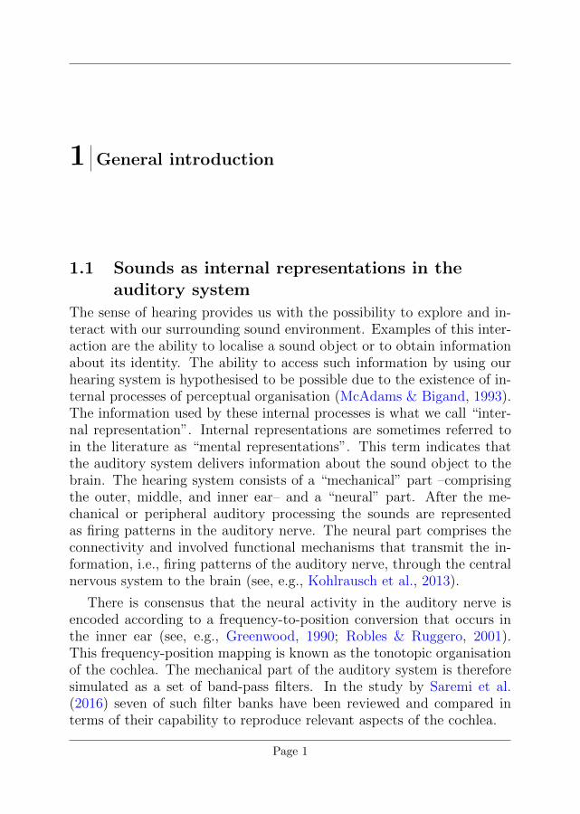
The sense of hearing provides us with the possibility to explore and in-teract with our surrounding sound environment. Examples of this inter-action are the ability to localise a sound object or to obtain informationabout its identity. The ability to access such information by using ourhearing system is hypothesised to be possible due to the existence of in-ternal processes of perceptual organisation (McAdams & Bigand, 1993).The information used by these internal processes is what we call “inter-nal representation”. Internal representations are sometimes referred toin the literature as “mental representations”. This term indicates thatthe auditory system delivers information about the sound object to thebrain. The hearing system consists of a “mechanical” part –comprisingthe outer, middle, and inner ear– and a “neural” part. After the me-chanical or peripheral auditory processing the sounds are representedas firing patterns in the auditory nerve. The neural part comprises theconnectivity and involved functional mechanisms that transmit the in-formation, i.e., firing patterns of the auditory nerve, through the centralnervous system to the brain (see, e.g., Kohlrausch et al., 2013).
There is consensus that the neural activity in the auditory nerve isencoded according to a frequency-to-position conversion that occurs inthe inner ear (see, e.g., Greenwood, 1990; Robles & Ruggero, 2001).This frequency-position mapping is known as the tonotopic organisationof the cochlea. The mechanical part of the auditory system is thereforesimulated as a set of band-pass filters. In the study by Saremi et al.(2016) seven of such filter banks have been reviewed and compared interms of their capability to reproduce relevant aspects of the cochlea.
Page 1
1 General introduction
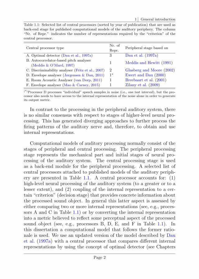
Table 1.1: Selected list of central processors (sorted by year of publication) that are used asback-end stage for published computational models of the auditory periphery. The column“Nr. of Repr.” indicates the number of representations required by the “criterion” of thecentral processor.
Central processor typeNr. of
Peripheral stage based onRepr.
A. Optimal detector (Dau et al., 1997a) 3 Dau et al. (1997a)B. Autocorrelator-based pitch analyser
1 Meddis and Hewitt (1991)(Meddis & O’Mard, 1997)
C. Discriminability analyser (Fritz et al., 2007) 2 Glasberg and Moore (2002)D. Envelope analyser (Jørgensen & Dau, 2011) 1∗ Ewert and Dau (2000)E. Room Acoustic Analyser (van Dorp, 2011) 1 Breebaart et al. (2001)F. Envelope analyser (Mao & Carney, 2015) 1 Zilany et al. (2009)
(*)Processor D processes “individual” speech samples in noise (i.e., one test interval), but the pro-cessor also needs to have access to the internal representation of the noise alone in order to generateits output metric.
In contrast to the processing in the peripheral auditory system, thereis no similar consensus with respect to stages of higher-level neural pro-cessing. This has generated diverging approaches to further process thefiring patterns of the auditory nerve and, therefore, to obtain and useinternal representations.
Computational models of auditory processing normally consist of thestages of peripheral and central processing. The peripheral processingstage represents the mechanical part and initial stages of neural pro-cessing of the auditory system. The central processing stage is usedas a back-end module for the peripheral processing. A selected list ofcentral processors attached to published models of the auditory periph-ery are presented in Table 1.1. A central processor accounts for: (1)high-level neural processing of the auditory system (to a greater or to alesser extent), and (2) coupling of the internal representation to a cer-tain “criterion” (decision stage) that provides concrete information aboutthe processed sound object. In general this latter aspect is assessed byeither comparing two or more internal representations (see, e.g., proces-sors A and C in Table 1.1) or by converting the internal representationinto a metric believed to reflect some perceptual aspect of the processedsound object (see, e.g., processors B, D, E, and F in Table 1.1). Inthis dissertation a computational model that follows the former ratio-nale is used. We use an updated version of the model described by Dauet al. (1997a) with a central processor that compares different internalrepresentations by using the concept of optimal detector (see Chapters
Page 2
1 General introduction
Ch
ap
ter
1
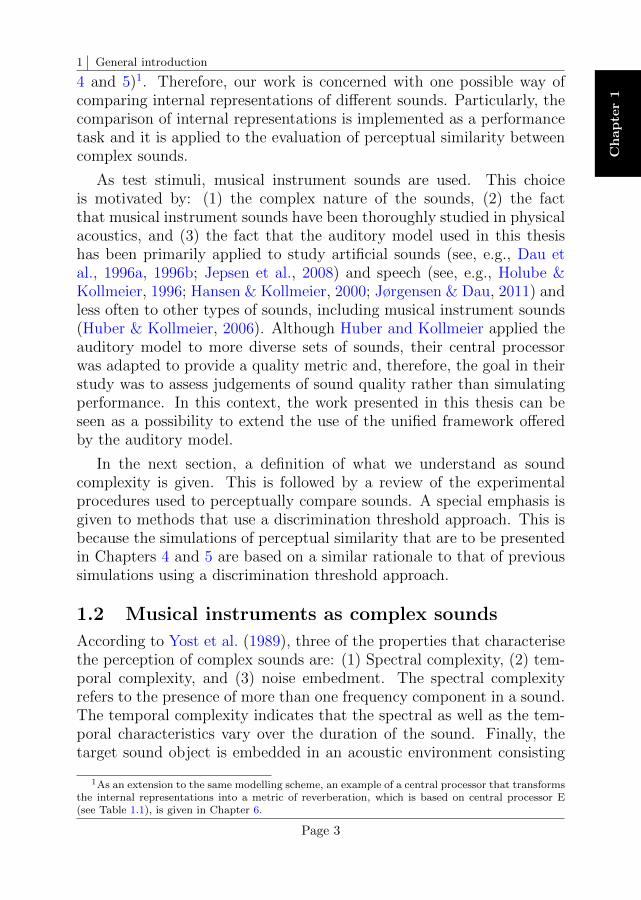
4 and 5)1. Therefore, our work is concerned with one possible way ofcomparing internal representations of different sounds. Particularly, thecomparison of internal representations is implemented as a performancetask and it is applied to the evaluation of perceptual similarity betweencomplex sounds.
As test stimuli, musical instrument sounds are used. This choiceis motivated by: (1) the complex nature of the sounds, (2) the factthat musical instrument sounds have been thoroughly studied in physicalacoustics, and (3) the fact that the auditory model used in this thesishas been primarily applied to study artificial sounds (see, e.g., Dau etal., 1996a, 1996b; Jepsen et al., 2008) and speech (see, e.g., Holube &Kollmeier, 1996; Hansen & Kollmeier, 2000; Jørgensen & Dau, 2011) andless often to other types of sounds, including musical instrument sounds(Huber & Kollmeier, 2006). Although Huber and Kollmeier applied theauditory model to more diverse sets of sounds, their central processorwas adapted to provide a quality metric and, therefore, the goal in theirstudy was to assess judgements of sound quality rather than simulatingperformance. In this context, the work presented in this thesis can beseen as a possibility to extend the use of the unified framework offeredby the auditory model.
In the next section, a definition of what we understand as soundcomplexity is given. This is followed by a review of the experimentalprocedures used to perceptually compare sounds. A special emphasis isgiven to methods that use a discrimination threshold approach. This isbecause the simulations of perceptual similarity that are to be presentedin Chapters 4 and 5 are based on a similar rationale to that of previoussimulations using a discrimination threshold approach.
1.2 Musical instruments as complex sounds
According to Yost et al. (1989), three of the properties that characterisethe perception of complex sounds are: (1) Spectral complexity, (2) tem-poral complexity, and (3) noise embedment. The spectral complexityrefers to the presence of more than one frequency component in a sound.The temporal complexity indicates that the spectral as well as the tem-poral characteristics vary over the duration of the sound. Finally, thetarget sound object is embedded in an acoustic environment consisting
1As an extension to the same modelling scheme, an example of a central processor that transformsthe internal representations into a metric of reverberation, which is based on central processor E(see Table 1.1), is given in Chapter 6.
Page 3
1 General introduction
of more objects. The “other objects” constitute a background noise thataffects directly or indirectly the sound object properties.
According to these definitions, the sets of sounds used throughoutthis dissertation are both spectrally and temporally complex. Since allthe stimuli correspond to recorded musical instruments and they arenoise-free, the role of noise embedment will not be addressed here. Noiseembedment will be used, however, to mask the properties of given targetsounds. Those noises are of stochastic nature, but have the same spectro-temporal characteristics as the target sounds. The generation of suchnoises is described in Chapters 3 and 5.
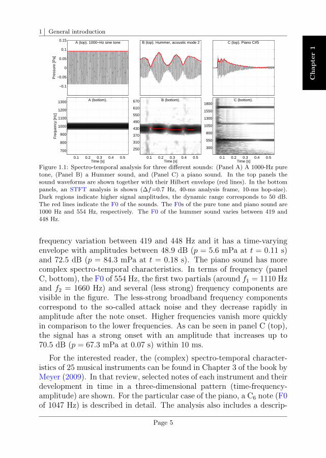
A spectro-temporal representation of three sounds is shown in Fig-ure 1.1. The sounds correspond to a 1000-Hz pure tone (panel A), arecording of an instrument called Hummer, resonating in its acousticmode 2 (panel B), and a recording of a piano sound, note C#5 (panelC). The Hummer corresponds to the test instrument studied in Chapter 2and the piano (note C#5) corresponds to the test instrument studied inChapters 3, 4, and 5. In the top panels of the figure the respective wave-forms (black lines) together with their Hilbert envelope (red lines) areshown. The envelope is used as a representation of the slow responseof the human hearing system to incoming sounds. This characteristic issometimes referred to as “sluggishness” of the hearing system. There-fore, a constant envelope can be interpreted as belonging to a steadysound. Likewise, an envelope that varies in time is attributed to a soundthat is perceived as a time-varying waveform. In the bottom panels ofFigure 1.1 a short-time Fourier transform (STFT)2 analysis is shown.Darker regions in the spectrogram represent higher signal amplitudes.Those amplitudes range between the maximum in the signal (darkestarea) down to a floor amplitude that is 50 dB below (white area). Thered lines indicate the estimated fundamental frequency (F0) of the sig-nals. The frequency range in each panel was chosen to facilitate thevisualisation of the relevant spectral components in the sounds.
According to our definition of complexity, the sounds in panels A,B, and C of Figure 1.1 have an increasing complexity. The sine toneconsists of a single spectral component at a frequency of 1000 Hz andits envelope is steady. The hummer sound has an F0 of 430 Hz, with a
2For the STFT analysis the waveforms were downsampled to an fs of 22050 Hz. The STFTis based on successive 32768-point FFTs performed on 40-ms signal segments (zero-padding wasapplied) with 75% overlap (10-ms hop size). The resulting frequency resolution of the analysis is0.7 Hz.
Page 4
1 General introduction
Ch
ap
ter
1
0.1 0.2 0.3 0.4 0.5
−0.1
−0.05
0
0.05
0.1
0.15 A (top). 1000−Hz sine tone
Time [s]
Pre
ssur
e [P
a]
0.1 0.2 0.3 0.4 0.5
B (top). Hummer, acoustic mode 2
Time [s]0.1 0.2 0.3 0.4 0.5
C (top). Piano C#5
Time [s]
Time [s]
Fre
quen
cy [H
z]
A (bottom).
0.1 0.2 0.3 0.4 0.5
700
800
900
1000
1100
1200
1300
Time [s]
B (bottom).
0.1 0.2 0.3 0.4 0.5
250
310
370
430
490
550
610
670
Time [s]
C (bottom).
0.1 0.2 0.3 0.4 0.5
300
550
800
1050
1300
1550
1800
Figure 1.1: Spectro-temporal analysis for three different sounds: (Panel A) A 1000-Hz puretone, (Panel B) a Hummer sound, and (Panel C) a piano sound. In the top panels thesound waveforms are shown together with their Hilbert envelope (red lines). In the bottompanels, an STFT analysis is shown (∆f=0.7 Hz, 40-ms analysis frame, 10-ms hop-size).Dark regions indicate higher signal amplitudes, the dynamic range corresponds to 50 dB.The red lines indicate the F0 of the sounds. The F0s of the pure tone and piano sound are1000 Hz and 554 Hz, respectively. The F0 of the hummer sound varies between 419 and448 Hz.
frequency variation between 419 and 448 Hz and it has a time-varyingenvelope with amplitudes between 48.9 dB (p = 5.6 mPa at t = 0.11 s)and 72.5 dB (p = 84.3 mPa at t = 0.18 s). The piano sound has morecomplex spectro-temporal characteristics. In terms of frequency (panelC, bottom), the F0 of 554 Hz, the first two partials (around f1 = 1110 Hzand f2 = 1660 Hz) and several (less strong) frequency components arevisible in the figure. The less-strong broadband frequency componentscorrespond to the so-called attack noise and they decrease rapidly inamplitude after the note onset. Higher frequencies vanish more quicklyin comparison to the lower frequencies. As can be seen in panel C (top),the signal has a strong onset with an amplitude that increases up to70.5 dB (p = 67.3 mPa at 0.07 s) within 10 ms.
For the interested reader, the (complex) spectro-temporal character-istics of 25 musical instruments can be found in Chapter 3 of the book byMeyer (2009). In that review, selected notes of each instrument and theirdevelopment in time in a three-dimensional pattern (time-frequency-amplitude) are shown. For the particular case of the piano, a C6 note (F0of 1047 Hz) is described in detail. The analysis also includes a descrip-
Page 5
1 General introduction
tion of how the intensity and the style of playing (legato and staccato,for note C3) affects the tone colour of the resulting sound. These aspectsmay also be applicable (but they are not discussed in this thesis) to ourtest piano recordings (note C#5), especially the description of the attacknoise given for C6 due to its proximity to the C#5 string (less than oneoctave difference).
1.3 Methods for the perceptual evaluation ofmusical sounds
In this section, we review the most relevant approaches used so far toevaluate aspects of sound perception applied to musical sounds. A moredetailed description is provided for those methods that have been directlyor indirectly used in this dissertation. Other comprehensive reviews ofexperimental methods used in psychophysics are given by McAdams andBigand (1993, Chapter 6) and by Kingdom and Prins (2016).
In line with the review given by McAdams and Bigand in the contextof classification and recognition of sound sources, the different experi-mental tasks can be grouped in one of the following types: (1) Discrim-ination, (2) Psychophysical rating scales, (3) Preference/similarity rat-ings, (4) Matching, (5) Classification, and (6) Identification. For each ofthese tasks one or more experimental methods can be used. Based on theexpected outcome of each method, the described tasks are either labelledas a “performance” or as an “appearance” method. This label respondsto whether the trial responses can be evaluated as “correct/incorrect”or not. In an appearance-based method, apparent magnitudes (that arerelative or absolute) along any specific dimension or stimulus attributeare collected.
1.3.1 DiscriminationCategory: Performance – threshold methods
In this task the participant is asked to differentiate between two or morestimuli. The percentage of correct responses is calculated for differentlevels of the independent variable. The task can be implemented as anm-alternative forced-choice (AFC) experiment. In an m-AFC experi-ment there are m intervals per trial and m alternatives from which theparticipant has to choose one. In a 2-AFC task, the participant needs anexplicit reference to the dimension being investigated and he/she has tobe somehow familiar with it. For instance, in a 2-AFC intensity discrim-ination task, the participant is asked: “Which of the two intervals does
Page 6
1 General introduction
Ch
ap
ter
1
sound more intense?” (see, e.g., Rabinowitz, 1970, intensity discrimina-tion with pure tones). In this case, it is expected that the participant isfamiliar with the concept of intensity. The implementation of the taskas a 3-AFC experiment opens the possibility to not explicitly ask theparticipant about the dimension being investigated. In the example ofintensity discrimination, the question may turn into “Which of the threeintervals does sound different?”.
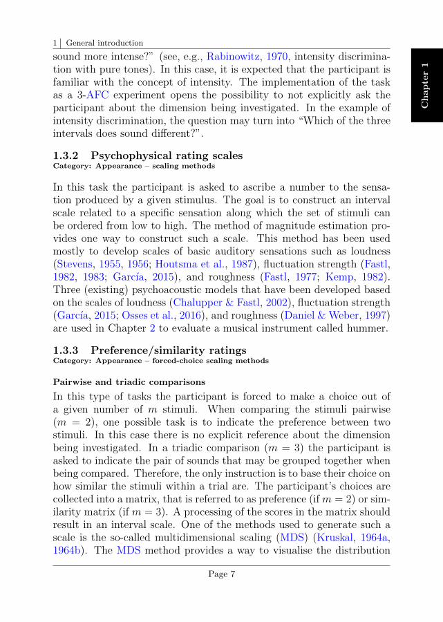
1.3.2 Psychophysical rating scalesCategory: Appearance – scaling methods
In this task the participant is asked to ascribe a number to the sensa-tion produced by a given stimulus. The goal is to construct an intervalscale related to a specific sensation along which the set of stimuli canbe ordered from low to high. The method of magnitude estimation pro-vides one way to construct such a scale. This method has been usedmostly to develop scales of basic auditory sensations such as loudness(Stevens, 1955, 1956; Houtsma et al., 1987), fluctuation strength (Fastl,1982, 1983; Garcıa, 2015), and roughness (Fastl, 1977; Kemp, 1982).Three (existing) psychoacoustic models that have been developed basedon the scales of loudness (Chalupper & Fastl, 2002), fluctuation strength(Garcıa, 2015; Osses et al., 2016), and roughness (Daniel & Weber, 1997)are used in Chapter 2 to evaluate a musical instrument called hummer.
1.3.3 Preference/similarity ratingsCategory: Appearance – forced-choice scaling methods
Pairwise and triadic comparisons
In this type of tasks the participant is forced to make a choice out ofa given number of m stimuli. When comparing the stimuli pairwise(m = 2), one possible task is to indicate the preference between twostimuli. In this case there is no explicit reference about the dimensionbeing investigated. In a triadic comparison (m = 3) the participant isasked to indicate the pair of sounds that may be grouped together whenbeing compared. Therefore, the only instruction is to base their choice onhow similar the stimuli within a trial are. The participant’s choices arecollected into a matrix, that is referred to as preference (if m = 2) or sim-ilarity matrix (if m = 3). A processing of the scores in the matrix shouldresult in an interval scale. One of the methods used to generate such ascale is the so-called multidimensional scaling (MDS) (Kruskal, 1964a,1964b). The MDS method provides a way to visualise the distribution
Page 7
1 General introduction
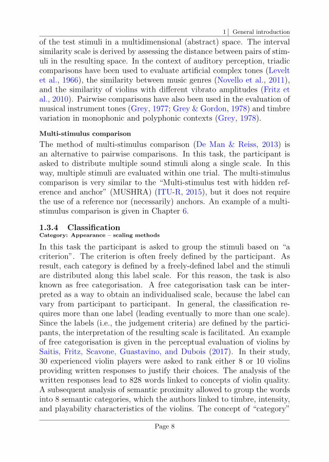
of the test stimuli in a multidimensional (abstract) space. The intervalsimilarity scale is derived by assessing the distance between pairs of stim-uli in the resulting space. In the context of auditory perception, triadiccomparisons have been used to evaluate artificial complex tones (Leveltet al., 1966), the similarity between music genres (Novello et al., 2011),and the similarity of violins with different vibrato amplitudes (Fritz etal., 2010). Pairwise comparisons have also been used in the evaluation ofmusical instrument tones (Grey, 1977; Grey & Gordon, 1978) and timbrevariation in monophonic and polyphonic contexts (Grey, 1978).
Multi-stimulus comparison
The method of multi-stimulus comparison (De Man & Reiss, 2013) isan alternative to pairwise comparisons. In this task, the participant isasked to distribute multiple sound stimuli along a single scale. In thisway, multiple stimuli are evaluated within one trial. The multi-stimuluscomparison is very similar to the “Multi-stimulus test with hidden ref-erence and anchor” (MUSHRA) (ITU-R, 2015), but it does not requirethe use of a reference nor (necessarily) anchors. An example of a multi-stimulus comparison is given in Chapter 6.
1.3.4 ClassificationCategory: Appearance – scaling methods
In this task the participant is asked to group the stimuli based on “acriterion”. The criterion is often freely defined by the participant. Asresult, each category is defined by a freely-defined label and the stimuliare distributed along this label scale. For this reason, the task is alsoknown as free categorisation. A free categorisation task can be inter-preted as a way to obtain an individualised scale, because the label canvary from participant to participant. In general, the classification re-quires more than one label (leading eventually to more than one scale).Since the labels (i.e., the judgement criteria) are defined by the partici-pants, the interpretation of the resulting scale is facilitated. An exampleof free categorisation is given in the perceptual evaluation of violins bySaitis, Fritz, Scavone, Guastavino, and Dubois (2017). In their study,30 experienced violin players were asked to rank either 8 or 10 violinsproviding written responses to justify their choices. The analysis of thewritten responses lead to 828 words linked to concepts of violin quality.A subsequent analysis of semantic proximity allowed to group the wordsinto 8 semantic categories, which the authors linked to timbre, intensity,and playability characteristics of the violins. The concept of “category”
Page 8
1 General introduction
Ch
ap
ter
1
is comparable to the concept of “dimension” of a perceptual space (thatcan be obtained with MDS) with the difference that the latter one is ofan abstract nature and requires further interpretation.
1.3.5 IdentificationCategory: Performance
In an identification or recognition task the participant is asked to link thetest stimuli with names or labels. The identification task can be basedon open-set labels (free identification) or on close-set labels. Possibleanalyses for an identification task are: (1) the assessment of identifica-tion scores (see, e.g., Saldanha & Corso, 1964), (2) the construction ofconfusion matrices (see, e.g., Steeneken, 1992, his Chapter 3), and (3)the measurement of reaction times (see, e.g., Agus et al., 2012).
In the study by Saldanha and Corso, notes of 10 musical instrumentswere recorded and presented in their original form and with 5 differenttypes of modification. The participants had to identify the instrumentbeing played based on a closed set of labels. Although the authors wereable to draw conclusions about the instruments that were easier to iden-tify and the type of modification that lead to a better performance,overall low scores per instrument were obtained (only three instrumentshad identification scores above 50%). The authors argued that a moreelaborate analysis of the incorrect scores would have provided furtherinformation to better explain their results. They indicated, for instance,that in most of the wrong answers for violin sounds, the cello had beenchosen and that this information could not be observed by only usingidentification scores. An analysis that can reflect this information is theconstruction of a confusion matrix. Such a matrix is constructed bycounting the number of times each stimulus is chosen over the other. Ahigh confusion score provides evidence of shared (perceptual) stimulusfeatures. In this way similarity can be implicitly evaluated. This givesthe possibility to analyse confusion matrices using techniques as principalcomponent component analysis (PCA) and MDS.
1.4 Linking methods of perceptual evaluation withauditory modelling frameworks
Our interest in this thesis is, as pointed out in Section 1.1, to evaluate thesimilarity between sounds by comparing their internal representationswhich, in turn, are derived from an auditory model (Dau et al., 1997a).
Page 9
1 General introduction
The decision stage of the model compares the internal representationsin terms of their spectro-temporal distribution of neural activity, whichis obtained from the corresponding sound intervals, usually presented in3-AFC trials.
In order to implement a similarity task using the same 3-AFC para-digm, the question to the participant needs to be implicitly asked. Oneway to do this would be to implement the experimental procedure as adiscrimination task (“which of the three sounds is different from theother two?”). Considering the definitions of the previous section, such atask corresponds to a performance task with forced choices. Other meth-ods that may be applicable to implement our similarity task are: themethod of triadic comparisons, and an identification task. The reasonsto favour the implementation of the similarity experiment as a discrimi-nation task over those methods are:
• The triadic comparison method is an appearance task, i.e., thereare “no wrong answers” in the similarity judgement;
• The similarity (distance) measure in the triadic comparisons de-pends on the choice of the set of stimuli, and;
• Although the participant’s performance can be assessed in an iden-tification task, this performance may also be influenced by the setof stimuli (or stimulus labels) chosen for the experiment.
Judgements of similarity in a 3-AFC discrimination task would onlydepend on the two sounds being compared (presented in three intervals)and will not be influenced by the “other” sound stimuli of the dataset.Additionally, the performance can be quantified by the percentage ofcorrect responses (scores), and the question “which of the three soundsis different from the other two?” can be evaluated by the auditory modelin terms of the spectro-temporal characteristics of each sound interval,under the assumption that similar sounds have similar spectro-temporalcharacteristics. If the discrimination task is implemented using an adap-tive procedure, the independent variable (the adjustable parameter) ischosen to influence the difficulty of the task, and discriminability thresh-olds can be obtained. An example of such an approach is the study onviolin sounds by Fritz et al. (2007), where the independent variable wasa gain applied to the test sound in four different frequency regions. Thislead to the estimation of four amplitude thresholds. They used an audi-tory model –the multichannel excitation-pattern model (Moore & Sek,
Page 10
1 General introduction
Ch
ap
ter
1
Musical instrument
A. Physicalmodelling
Numerical models
B. Listening C. Computational
listening
Auditory perception
D. Perceptualmodelling
Models of auditory perception
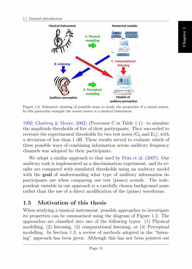
Figure 1.2: Schematic drawing of possible steps to study the properties of a sound source.In this particular example the sound source is a musical instrument.
1992; Glasberg & Moore, 2002) (Processor C in Table 1.1)– to simulatethe amplitude thresholds of five of their participants. They succeeded torecreate the experimental thresholds for two test notes (G3 and E5), witha deviation of less than 1 dB. These results served to evaluate which ofthree possible ways of combining information across auditory frequencychannels was adopted by their participants.
We adopt a similar approach to that used by Fritz et al. (2007). Ourauditory task is implemented as a discrimination experiment, and its re-sults are compared with simulated thresholds using an auditory modelwith the goal of understanding what type of auditory information doparticipants use when comparing our test (piano) sounds. The inde-pendent variable in our approach is a carefully chosen background noiserather than the use of a direct modification of the (piano) waveforms.
1.5 Motivation of this thesis
When studying a musical instrument, possible approaches to investigateits properties can be summarised using the diagram of Figure 1.2. Theapproaches are classified into one of the following types: (1) Physicalmodelling, (2) listening, (3) computational listening, or (4) Perceptualmodelling. In Section 1.3, a review of methods adopted in the “listen-ing” approach has been given. Although this has not been pointed out
Page 11
1 General introduction
so far, due to the (on average) long time required to conduct listen-ing experiments, an alternative is to use the approach that we labelledas “computational listening”, which represents the use of acoustic orpsychoacoustic metrics obtained from dedicated computer programs. Avery simple example of computational listening is the comparison of twoSTFTs. A more elaborate example is given by the acoustic similaritymetric of Agus et al. (2012), which is based on an energy average using asimplified internal representation of the sounds (Moore, 2003). The au-thors used this information to explain the results of their identificationtest, where shorter reaction times were found when the task consideredless similar sounds.
The “physical modelling” approach relies on the simulation of a soundsource by implementing a model for its vibration and sound radiation.Two examples of this approach in the study of guitar and piano soundsare given by Derveaux, Chaigne, Joly, and Becache (2003) and Chabassier,Chaigne, and Joly (2013). In order to evaluate how well does a givennumerical model match –or how similar the simulated sounds are to–the sound source under evaluation, a comparison with actual recordingsshould be conducted. The comparison can be done by either running lis-tening experiments (“listening”) or by applying some kind of computeranalysis (“computational listening”).
The remaining part of the diagram, i.e., the “perceptual modelling”approach, constitutes the main goal of this thesis. This approach con-sists of gaining insights into human performance –in our case, into “howdiscriminable” two sounds are– by incorporating advanced perceptualaspects into a computational listening approach. We compare experi-mental thresholds with simulated (or “perceptually modelled”) thresh-olds obtained from an auditory model. The test sounds in our task areindividual piano notes (Chapters 3 to 5). As an “acoustic event”, in-dividual notes are considered to be one of the simplest cases to study(McAdams & Bigand, 1993) when compared with the use of melodiclines or a fragment of music with multiple instruments. Our efforts arefocused, however, on the complex nature of the piano sounds and ona detailed analysis of their (multidimensional) internal representationsobtained from an auditory model. This model corresponds to an up-dated version of the perception model (PEMO) described by Dau et al.(1997a). As a consequence of using the PEMO model to assess simu-lated thresholds for complex (piano) sounds, the work in this thesis canbe seen as a further extension of this unified modelling framework that
Page 12
1 General introduction
Ch
ap
ter
1
has already been successful in simulating human performance in a rangeof auditory tasks.
1.6 Outline
In Chapter 2 a selection of psychoacoustic descriptors is reviewed andapplied to a set of sounds. The descriptors correspond to the classicpsychoacoustic measures of loudness, roughness and fluctuation strength.The descriptors are used to compare sounds of a musical instrumentcalled hummer. The hummer is a plastic corrugated pipe that generatessounds when being rotated at specific speeds. In this chapter existingrecordings of the hummer (Hirschberg et al., 2013) are quantitativelycompared with a computational model of the hummer (Nakiboglu et al.,2012). This study case corresponds to an example of the “computationallistening” approach shown in the schema of Figure 1.2, with as result anevaluation of the numerical model of the instrument.
In Chapter 3 an experimental method to assess the perceptual simi-larity among sounds is presented. The experimental method correspondsto an “instrument”-in-noise discrimination test where the noise is usedto manipulate the difficulty of the discrimination. The method of triadiccomparisons –largely used in psychology– is used as reference method.A perceptual similarity study using recorded piano sounds of one noteplayed on a number of historical pianos is presented. The instrument-in-noise method provides discrimination thresholds, expressed as signal-to-noise ratio (SNR), that are significantly correlated with the Euclideandistances between pianos in the perceptual space constructed from thetriadic comparisons. The listening experiments discussed in this chap-ter are an example of the “listening” approach shown in the schema ofFigure 1.2.
In Chapter 4 the perceptual similarity among sounds is simulated us-ing a computational model of the effective processing of the auditorysystem. The sounds are “presented” to the model in exactly the sameway as in the instrument-in-noise test validated in the previous chapter.The simulated thresholds are significantly correlated with the experimen-tal thresholds, when only a portion (onset) of the sounds is used as inputto the model. These results suggest that the auditory cues available inthe starting part of the sounds are sufficient to reach human perfor-mance with the model. The content of this chapter is an example of the“perceptual modelling” approach shown in the schema of Figure 1.2.
Page 13

1 General introduction
With the aim of broadening the use of the computational model ofChapter 4 to a different acoustic environment, in Chapter 5 the com-putational model is used to simulate the similarity of piano sounds in areverberant condition. The reverberation is applied to the same pianosounds used in Chapters 3 and 4 by means of digital convolution. Theeffect of reverberation on the piano sounds introduces a moderate changein their relative position in the perceptual similarity space. The exper-imental results of the instrument-in-noise test as well as the simulatedresults from the computational model also account for this change.
In Chapter 6 a computational model (Processor E in Table 1.1) similarto that of the previous chapters is used to simulate the perceived rever-beration of different orchestra instrument sounds in 8 different acousticenvironments. The model is set-up in a binaural configuration and adifferent central processor is used to generate reverberance estimates.Experimental results for the same instrument sounds are provided. Thereverberance estimates of the model for within-instrument conditions arecorrelated with the experimental results. This study case correspondsto an example of the “computational listening” approach shown in theschema of Figure 1.2.
In Chapter 7 the results and conclusions drawn from each chapterare briefly summarised. We discuss the context in which the auditorymodelling approach was used, including perspectives for further research.This discussion is centred on further improvements that could be intro-duced to the auditory model and their possible implications in the unifiedcomputational framework.
Page 14
2 Perceptual evaluation of instrument soundsusing classic psychoacoustic descriptors1
2.1 IntroductionOne way to better understand the properties of a musical instrument isto compare sound recordings of that instrument in controlled situationswith synthesised sounds generated with physical models that recreatesuch situations. These sounds can be compared adopting a “computa-tional listening” approach (see Figure 1.2 of the previous chapter). Sincemusical sounds are received and processed by the human hearing system,the comparison between sounds should be ideally based on perceptualcriteria.
Studies in the field of psychoacoustics have addressed the problem ofsound perception by developing (psychoacoustic) audio descriptors. Aspointed out in the previous chapter (see Section 1.3.2), this developmenthas been done by fitting algorithms of sound processing to experimentaldata obtained primarily with artificial test stimuli using the method ofmagnitude estimation (Stevens, 1955; Fastl, 1977; Zwicker, 1977; Kemp,1982; Fastl, 1982, 1983; Daniel & Weber, 1997). These metrics havealso been used to analyse other types of sounds such as speech, music,soundscapes, and sounds for product design (see, e.g., Terhardt, 1978;Genuit, 1997; Widmann, 1997; Yang & Kang, 2013).
In this chapter we compare recorded and synthesised sounds of aninstrument called hummer, also known as the “voice of the dragon”.
1This chapter is largely based on:A. Osses, R. Kim, and A. Kohlrausch (2015). “Perceptual evaluation of differences between originaland synthesised musical instrument sounds: the role of room acoustics”. Proceedings of EuroNoise.C. Glorieux (Ed.), pp. 2561–2566. Maastricht, the Netherlands.A. Osses, and A. Kohlrausch (2014). Perceptual evaluation of differences between original andsynthesised musical instrument sounds. Actas 9th Iberoamerican Congress on Acoustics FIA. J.Arenas (Ed.) pp. 987–997. Valdivia, Chile.
Page 15

2 Perceptual evaluation of instrument sounds using classic psychoacoustic descriptors
The comparison is done using classic psychoacoustic metrics –loudness(loudness fluctuations), roughness, fluctuation strength– applied to hum-mer sounds available from a previous research project (Nakiboglu et al.,2012; Hirschberg et al., 2013), where no quantitative evaluation of theagreement between their synthesised and recorded sounds was reported.Another motivation to evaluate hummer sounds is their simple nature:the sounds contain mainly one tonal component that oscillates period-ically in frequency and amplitude (see panel B of Figure 1.1, page 5).Additionally, the envelope of the sounds is not perfectly regular, havinga slowly-varying pattern in time. The aim of this chapter is, therefore,to compare available sounds of this simple musical instrument (recordedand synthesised) using quantitative evaluation criteria based on existingpsychoacoustic metrics.
Since the evaluation criteria are based on applying the concepts ofloudness, loudness fluctuations, roughness and fluctuation strength, westart the chapter by describing relevant aspects of these descriptors. Inaddition to these descriptors, F0 estimates are used to evaluate pitchvariations in the test sounds. During the analysis, particular emphasisis given to the sensations of fluctuation strength and roughness. Thesedescriptors characterise temporal fluctuations in amplitude and in fre-quency and are found naturally in everyday sounds.
2.2 Description of the methodThe evaluation between sounds is done by comparing a number of fea-tures extracted from each of the sounds. To add a perceptual compo-nent, a set of psychoacoustic descriptors is used to extract those soundfeatures. A summary of the descriptors used in this chapter is presentedin Table 2.1. Further details are described in the subsequent sections.
Descriptors 1-2: Loudness and loudness fluctuationsLoudness corresponds to the perceptual correlate of the sound pressurelevel and is expressed in sone. The reference sound producing 1 soneis a 1-kHz sine tone with an SPL of 40 dB. A level increase of 10 dBleads roughly to a doubling of the loudness of a sound. In this chap-ter the loudness is obtained from the dynamic loudness model (DLM)(Chalupper & Fastl, 2002). This model provides loudness estimates as afunction of time and frequency.
In order to appropriately describe the concept of loudness fluctuations,we need to introduce a more detailed description of the DLM model. The
Page 16
2 Perceptual evaluation of instrument sounds using classic psychoacoustic descriptors
Ch
ap
ter
2
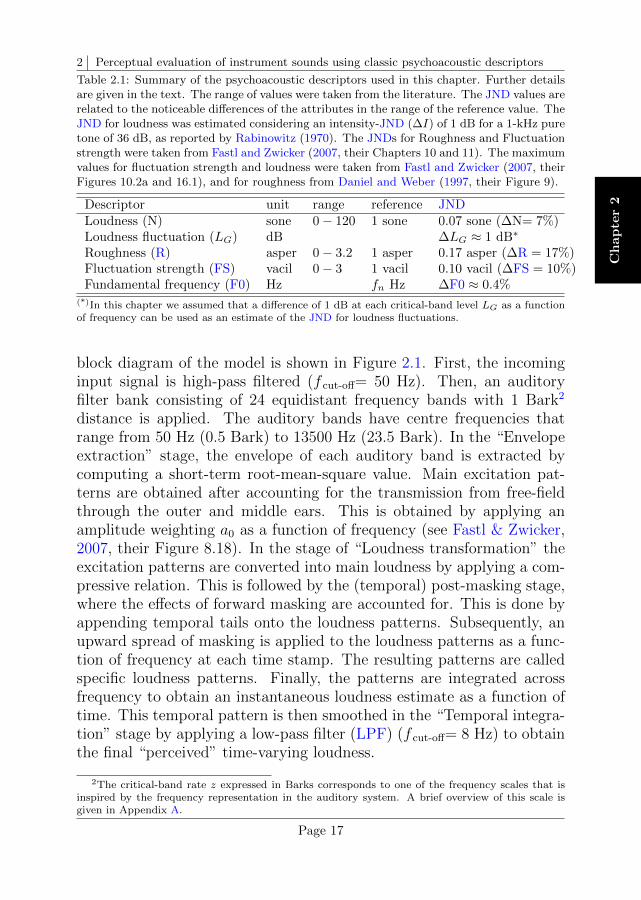
Table 2.1: Summary of the psychoacoustic descriptors used in this chapter. Further detailsare given in the text. The range of values were taken from the literature. The JND values arerelated to the noticeable differences of the attributes in the range of the reference value. TheJND for loudness was estimated considering an intensity-JND (∆I) of 1 dB for a 1-kHz puretone of 36 dB, as reported by Rabinowitz (1970). The JNDs for Roughness and Fluctuationstrength were taken from Fastl and Zwicker (2007, their Chapters 10 and 11). The maximumvalues for fluctuation strength and loudness were taken from Fastl and Zwicker (2007, theirFigures 10.2a and 16.1), and for roughness from Daniel and Weber (1997, their Figure 9).
Descriptor unit range reference JNDLoudness (N) sone 0− 120 1 sone 0.07 sone (∆N= 7%)Loudness fluctuation (LG) dB ∆LG ≈ 1 dB∗
Roughness (R) asper 0− 3.2 1 asper 0.17 asper (∆R = 17%)Fluctuation strength (FS) vacil 0− 3 1 vacil 0.10 vacil (∆FS = 10%)Fundamental frequency (F0) Hz fn Hz ∆F0 ≈ 0.4%
(*)In this chapter we assumed that a difference of 1 dB at each critical-band level LG as a functionof frequency can be used as an estimate of the JND for loudness fluctuations.
block diagram of the model is shown in Figure 2.1. First, the incominginput signal is high-pass filtered (f cut-off= 50 Hz). Then, an auditoryfilter bank consisting of 24 equidistant frequency bands with 1 Bark2
distance is applied. The auditory bands have centre frequencies thatrange from 50 Hz (0.5 Bark) to 13500 Hz (23.5 Bark). In the “Envelopeextraction” stage, the envelope of each auditory band is extracted bycomputing a short-term root-mean-square value. Main excitation pat-terns are obtained after accounting for the transmission from free-fieldthrough the outer and middle ears. This is obtained by applying anamplitude weighting a0 as a function of frequency (see Fastl & Zwicker,2007, their Figure 8.18). In the stage of “Loudness transformation” theexcitation patterns are converted into main loudness by applying a com-pressive relation. This is followed by the (temporal) post-masking stage,where the effects of forward masking are accounted for. This is done byappending temporal tails onto the loudness patterns. Subsequently, anupward spread of masking is applied to the loudness patterns as a func-tion of frequency at each time stamp. The resulting patterns are calledspecific loudness patterns. Finally, the patterns are integrated acrossfrequency to obtain an instantaneous loudness estimate as a function oftime. This temporal pattern is then smoothed in the “Temporal integra-tion” stage by applying a low-pass filter (LPF) (f cut-off= 8 Hz) to obtainthe final “perceived” time-varying loudness.
2The critical-band rate z expressed in Barks corresponds to one of the frequency scales that isinspired by the frequency representation in the auditory system. A brief overview of this scale isgiven in Appendix A.
Page 17

2 Perceptual evaluation of instrument sounds using classic psychoacoustic descriptors
Figure 2.1: Block diagram of the DLM model. The model is briefly described in the text.
As an estimate of the loudness fluctuation of a sound, the critical-bandlevels LG are used. They correspond to a representation of the envelopeof the sound in dB as a function of frequency. In order to obtain criticalband levels LG that account for the temporal and spectral masking, thestages of “Loudness transformation” and “Transmission factor a0” arereversed using the low-pass filtered specific loudness patterns. This isindicated in Figure 2.1 by the arrows in the lower part of the diagram.The reversed stages are highlighted in the diagram. The resulting LGlevels are labelled as “Critical band level LG (+masking)” in the dia-gram. The minimum and maximum level patterns are estimated fromthe percentiles 5 and 95, respectively. Since the analysis presented in thischapter considers only “short signals” of 1.2 s (hummer sound, acousticmode 2) or less, these percentiles are assessed over the entire duration ofthe sounds.
Descriptor 3: RoughnessRoughness (R) is a metric that describes how “rough” a sound is and iscaused by the presence of rapid amplitude and/or frequency modulationswith modulation rates between 15 and 300 Hz. The sensation of “rough-ness” has a bandpass characteristic with a maximum near the frequencyof 70 Hz. Roughness is expressed in asper, where a sound producing 1asper corresponds to a 1-kHz sine tone, 100% sinusoidally amplitude-modulated, with a modulation frequency of 70 Hz and an SPL of 60 dB(Kemp, 1982; Daniel & Weber, 1997). The lower limit of roughnessperception is 0.07 asper and several authors agree that a relative varia-tion of about 17% elicits a just-noticeable change in roughness (Vogel,1975; Daniel & Weber, 1997; Fastl & Zwicker, 2007, Chapter 11). Themodel described by Daniel and Weber (1997) is used in this chapter.Particularly, we used the model outputs of main roughness and specificroughness.
Descriptor 4: Fluctuation strengthThe metric of fluctuation strength (FS) is used to describe slow ampli-tude and/or frequency modulations with modulation rates below 20 Hz.
Page 18
2 Perceptual evaluation of instrument sounds using classic psychoacoustic descriptors
Ch
ap
ter
2
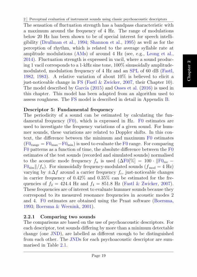
The sensation of fluctuation strength has a bandpass characteristic witha maximum around the frequency of 4 Hz. The range of modulationsbelow 20 Hz has been shown to be of special interest for speech intelli-gibility (Drullman et al., 1994; Shannon et al., 1995) as well as for theperception of rhythm, which is related to the average syllable rate atamplitude modulations (AMs) of around 4 Hz (see, e.g., Leong et al.,2014). Fluctuation strength is expressed in vacil, where a sound produc-ing 1 vacil corresponds to a 1-kHz sine tone, 100% sinusoidally amplitude-modulated, modulation frequency of 4 Hz and an SPL of 60 dB (Fastl,1982, 1983). A relative variation of about 10% is believed to elicit ajust-noticeable change in FS (Fastl & Zwicker, 2007, their Chapter 10).The model described by Garcıa (2015) and Osses et al. (2016) is used inthis chapter. This model has been adapted from an algorithm used toassess roughness. The FS model is described in detail in Appendix B.
Descriptor 5: Fundamental frequencyThe periodicity of a sound can be estimated by calculating the fun-damental frequency (F0), which is expressed in Hz. F0 estimates areused to investigate the frequency variations of a given sound. For hum-mer sounds, these variations are related to Doppler shifts. In this con-text, the difference between the minimum and maximum F0 estimates(F0range = F0max−F0min) is used to evaluate the F0 range. For comparingF0 patterns as a function of time, the absolute difference between the F0estimates of the test sounds (recorded and simulated sounds) normalisedto the acoustic mode frequency fn is used (∆F0[%] = 100 · ‖F0rec −F0sim‖/fn). For sinusoidally frequency-modulated sounds (fmod = 4 Hz)varying by ±∆f around a carrier frequency fc, just-noticeable changesin carrier frequency of 0.42% and 0.35% can be estimated for the fre-quencies of f2 = 424.4 Hz and f4 = 851.8 Hz (Fastl & Zwicker, 2007).These frequencies are of interest to evaluate hummer sounds because theycorrespond to its measured resonance frequencies in acoustic modes 2and 4. F0 estimates are obtained using the Praat software (Boersma,1993; Boersma & Weenink, 2001).
2.2.1 Comparing two soundsThe comparisons are based on the use of psychoacoustic descriptors. Foreach descriptor, test sounds differing by more than a minimum detectablechange (one JND), are labelled as different enough to be distinguishedfrom each other. The JNDs for each psychoacoustic descriptor are sum-marised in Table 2.1.
Page 19
2 Perceptual evaluation of instrument sounds using classic psychoacoustic descriptors
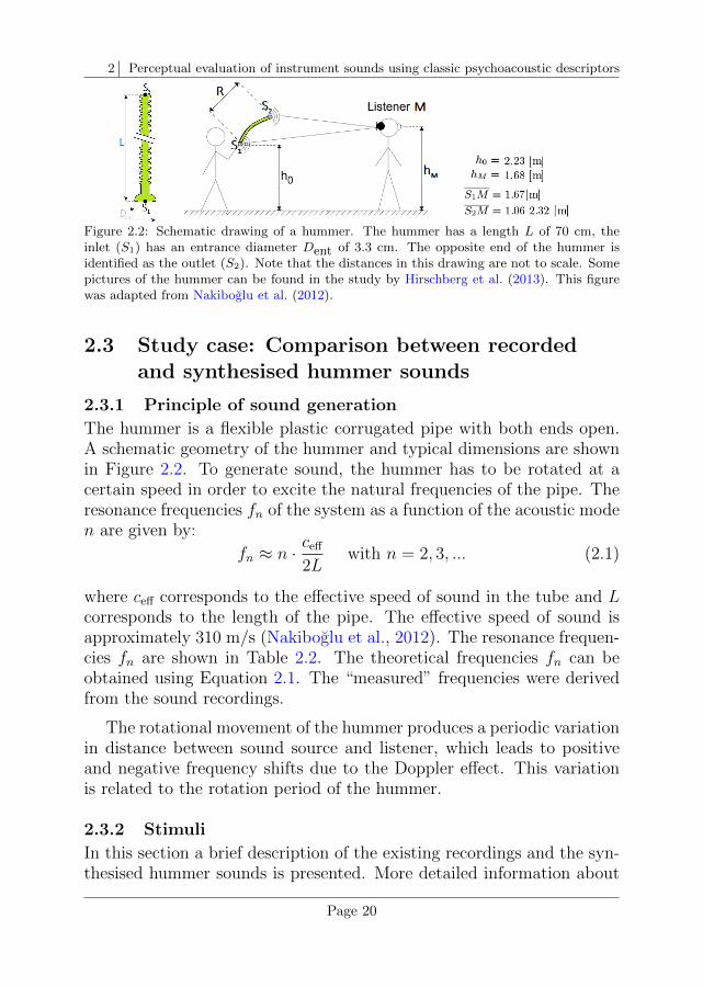
Figure 2.2: Schematic drawing of a hummer. The hummer has a length L of 70 cm, theinlet (S1) has an entrance diameter Dent of 3.3 cm. The opposite end of the hummer isidentified as the outlet (S2). Note that the distances in this drawing are not to scale. Somepictures of the hummer can be found in the study by Hirschberg et al. (2013). This figurewas adapted from Nakiboglu et al. (2012).
2.3 Study case: Comparison between recordedand synthesised hummer sounds
2.3.1 Principle of sound generation
The hummer is a flexible plastic corrugated pipe with both ends open.A schematic geometry of the hummer and typical dimensions are shownin Figure 2.2. To generate sound, the hummer has to be rotated at acertain speed in order to excite the natural frequencies of the pipe. Theresonance frequencies fn of the system as a function of the acoustic moden are given by:
fn ≈ n · ceff
2Lwith n = 2, 3, ... (2.1)
where ceff corresponds to the effective speed of sound in the tube and Lcorresponds to the length of the pipe. The effective speed of sound isapproximately 310 m/s (Nakiboglu et al., 2012). The resonance frequen-cies fn are shown in Table 2.2. The theoretical frequencies fn can beobtained using Equation 2.1. The “measured” frequencies were derivedfrom the sound recordings.
The rotational movement of the hummer produces a periodic variationin distance between sound source and listener, which leads to positiveand negative frequency shifts due to the Doppler effect. This variationis related to the rotation period of the hummer.
2.3.2 Stimuli
In this section a brief description of the existing recordings and the syn-thesised hummer sounds is presented. More detailed information about
Page 20

2 Perceptual evaluation of instrument sounds using classic psychoacoustic descriptors
Ch
ap
ter
2
Table 2.2: Resonance frequency fn and rotation period Ωn for the hummer at differentrotation speeds (modes 2 and 4) derived from both, theory (Equation 2.1) and the recordings.
Acoustic Frequency fn [Hz] ∆F0 Periodmode n Theory Measured [%] Ωn [s]
2 442.9 424.4 4.2 0.6024 885.7 851.8 3.8 0.296
the mechanical measurement set-up used for the sound recordings is givenby Hirschberg et al. (2013). The physical model used for synthesisingthe hummer sounds is described by Nakiboglu et al. (2012).
Recorded sounds
The recordings were made using a mechanical set-up, where the hummerwas attached to a bicycle wheel with an adjustable rotation speed. Theset-up was installed in a semi-anechoic room (volume of 100 m3) that hada non-reflecting floor. The resulting environment was nearly anechoic.This means that the microphone M captured only contributions from thesources S1 and S2. Figure 2.2 gives a schematic view of the position ofthe hummer with respect to the microphone M . The mechanical systemon which the hummer was mounted is not shown in the figure.
The hummer was attached to the spikes of a 26” bicycle wheel. Theinlet S1 was placed close to the axis of rotation (wheel axis). The outletS2 was at a distance of 0.70 m from the wheel axis, approximately 0.30 moutside the radius of the wheel. The wheel was mounted on a structure(oriented horizontally), at a height of 2.23 m above the floor. The wheelaxis was defined to be at coordinates (0,0,2.23) m.
A microphone B&K type 4190, located at (1.58, 0, 1.68) m, was usedto record the hummer. The microphone was located, thus, at a distanceof 1.67 m from the centre of rotation. Each recording had a durationof 20 s and was sampled at 10 kHz, with an amplitude resolution of 16bits. The measured resonance frequencies differed by about 4% from theapproximation given by Equation 2.1, as shown in Table 2.2.
The recorded signals were re-sampled at 44.1 kHz, with an amplituderesolution of 16 bits. The average level was adjusted according to thereference levels of 54 and 72 dB SPL at 1.67 m from the origin of thesystem for the acoustic modes 2 and 4, respectively.
The waveforms of the recorded hummer signals as used in this chapterare shown in panel A of Figure 2.3. As a consequence of the movement
Page 21
2 Perceptual evaluation of instrument sounds using classic psychoacoustic descriptors
−0.02
0
0.02
Pre
ssu
re [
Pa
] A (left). Recorded hummer, ac. mode 2
−0.02
0
0.02
Pre
ssu
re [
Pa
] B (left). Synthesised hummer, ac. mode 2
410
420
430
440
Fre
qu
en
cy [
Hz] C (left). Fundamental frequency F0
0.2 0.4 0.6 0.8 1 1.2
−2
0
2
4
6
∆ f
/fn [
%]
D (left). ∆ F0
Time [s]
−0.2
0
0.2
Pre
ssu
re [
Pa
] A (right). Recorded hummer, ac. mode 4
−0.2
0
0.2
Pre
ssu
re [
Pa
] B (right). Synthesised hummer, ac. mode 4
820
840
860
880
Fre
qu
en
cy [
Hz] C (right). Fundamental frequency F0
2.7 2.8 2.9 3 3.1 3.2 3.3
−2
0
2
4
6
∆ f
/fn [
%]
D (right). ∆ F0
Time [s]
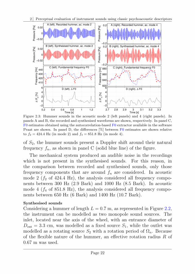
Figure 2.3: Hummer sounds in the acoustic mode 2 (left panels) and 4 (right panels). Inpanels A and B, the recorded and synthesised waveforms are shown, respectively. In panel C,F0 estimates obtained using the autocorrelation-based F0 extractor available in the softwarePraat are shown. In panel D, the differences [%] between F0 estimates are shown relativeto f2 = 424.4 Hz (in mode 2) and f4 = 851.8 Hz (in mode 4).
of S2, the hummer sounds present a Doppler shift around their naturalfrequency fn, as shown in panel C (solid blue line) of the figure.
The mechanical system produced an audible noise in the recordingswhich is not present in the synthesised sounds. For this reason, inthe comparison between recorded and synthesised sounds, only thosefrequency components that are around fn are considered. In acousticmode 2 (f2 of 424.4 Hz), the analysis considered all frequency compo-nents between 300 Hz (2.9 Bark) and 1000 Hz (8.5 Bark). In acousticmode 4 (f4 of 851.8 Hz), the analysis considered all frequency compo-nents between 650 Hz (6 Bark) and 1400 Hz (10.7 Bark).
Synthesised sounds
Considering a hummer of length L = 0.7 m, as represented in Figure 2.2,the instrument can be modelled as two monopole sound sources. Theinlet, located near the axis of the wheel, with an entrance diameter ofDent = 3.3 cm, was modelled as a fixed source S1, while the outlet wasmodelled as a rotating source S2 with a rotation period of Ωn. Becauseof the flexible nature of the hummer, an effective rotation radius R of0.67 m was used.
Page 22
2 Perceptual evaluation of instrument sounds using classic psychoacoustic descriptors
Ch
ap
ter
2
0.2 0.4 0.6 0.8 1 1.2
11.21.41.61.8
22.22.42.62.8
33.2
Time [s]
Lo
ud
ne
ss [
so
ne
]
A. Hummer, acoustic mode 2
2.7 2.8 2.9 3 3.1 3.2 3.3
3
3.5
4
4.5
5
5.5
6
6.5
Time [s]
Lo
ud
ne
ss [
so
ne
]
B. Hummer, acoustic mode 4
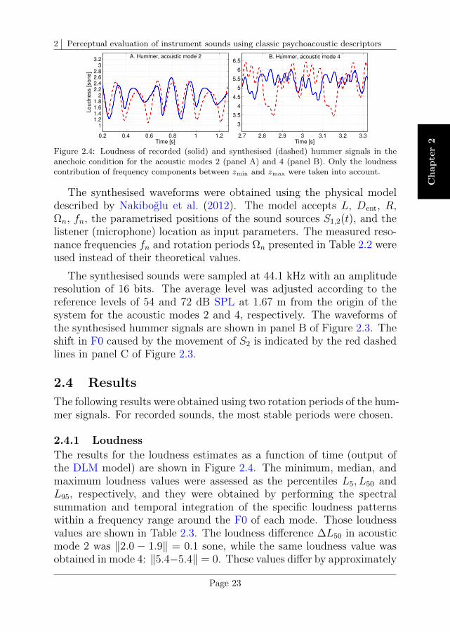
Figure 2.4: Loudness of recorded (solid) and synthesised (dashed) hummer signals in theanechoic condition for the acoustic modes 2 (panel A) and 4 (panel B). Only the loudnesscontribution of frequency components between zmin and zmax were taken into account.
The synthesised waveforms were obtained using the physical modeldescribed by Nakiboglu et al. (2012). The model accepts L, Dent, R,Ωn, fn, the parametrised positions of the sound sources S1,2(t), and thelistener (microphone) location as input parameters. The measured reso-nance frequencies fn and rotation periods Ωn presented in Table 2.2 wereused instead of their theoretical values.
The synthesised sounds were sampled at 44.1 kHz with an amplituderesolution of 16 bits. The average level was adjusted according to thereference levels of 54 and 72 dB SPL at 1.67 m from the origin of thesystem for the acoustic modes 2 and 4, respectively. The waveforms ofthe synthesised hummer signals are shown in panel B of Figure 2.3. Theshift in F0 caused by the movement of S2 is indicated by the red dashedlines in panel C of Figure 2.3.
2.4 Results
The following results were obtained using two rotation periods of the hum-mer signals. For recorded sounds, the most stable periods were chosen.
2.4.1 Loudness
The results for the loudness estimates as a function of time (output ofthe DLM model) are shown in Figure 2.4. The minimum, median, andmaximum loudness values were assessed as the percentiles L5, L50 andL95, respectively, and they were obtained by performing the spectralsummation and temporal integration of the specific loudness patternswithin a frequency range around the F0 of each mode. Those loudnessvalues are shown in Table 2.3. The loudness difference ∆L50 in acousticmode 2 was ‖2.0 − 1.9‖ = 0.1 sone, while the same loudness value wasobtained in mode 4: ‖5.4−5.4‖ = 0. These values differ by approximately
Page 23
2 Perceptual evaluation of instrument sounds using classic psychoacoustic descriptors
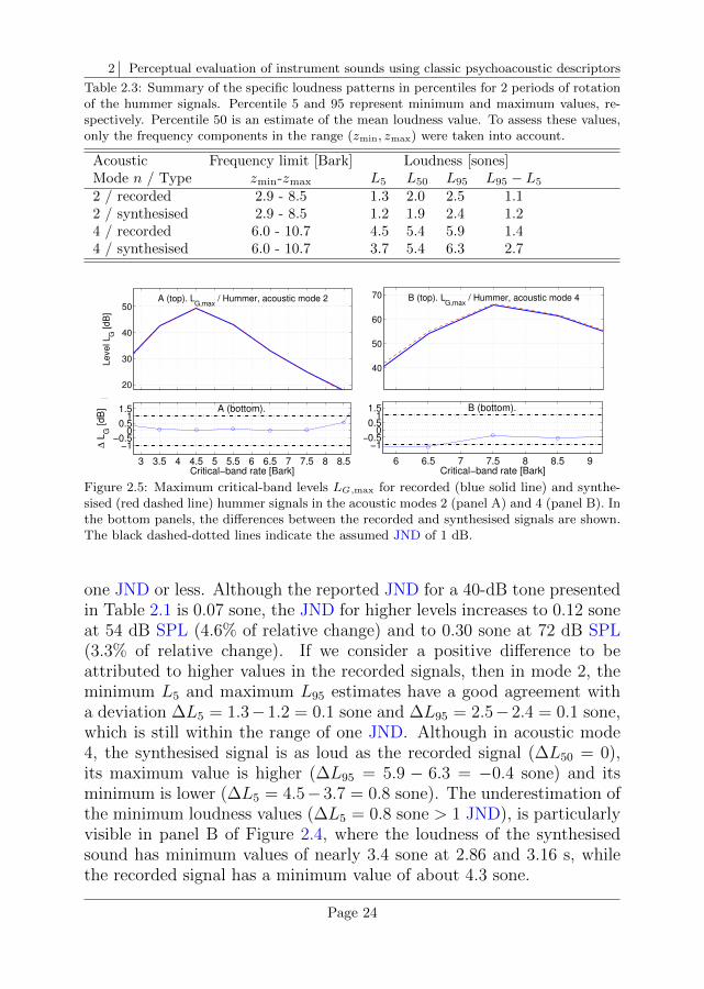
Table 2.3: Summary of the specific loudness patterns in percentiles for 2 periods of rotationof the hummer signals. Percentile 5 and 95 represent minimum and maximum values, re-spectively. Percentile 50 is an estimate of the mean loudness value. To assess these values,only the frequency components in the range (zmin, zmax) were taken into account.
Acoustic Frequency limit [Bark] Loudness [sones]Mode n / Type zmin-zmax L5 L50 L95 L95 − L5
2 / recorded 2.9 - 8.5 1.3 2.0 2.5 1.12 / synthesised 2.9 - 8.5 1.2 1.9 2.4 1.24 / recorded 6.0 - 10.7 4.5 5.4 5.9 1.44 / synthesised 6.0 - 10.7 3.7 5.4 6.3 2.7
20
30
40
50
Le
ve
l L
G [
dB
]
A (top). LG,max
/ Hummer, acoustic mode 2
3 3.5 4 4.5 5 5.5 6 6.5 7 7.5 8 8.5
−0.5
0
0.5
1
∆ L
G [
dB
]
Critical−band rate [Bark]
A (bottom).
40
50
60
70
Le
ve
l L
G [
dB
]
B (top). LG,max
/ Hummer, acoustic mode 4
6 6.5 7 7.5 8 8.5 9
−1.5
−1
−0.5
0
∆ L
G [
dB
]
Critical−band rate [Bark]
B (bottom).
20
40
Level L
G [dB
]
A (top). LG,max
/ Hummer, acoustic mode 2
3 3.5 4 4.5 5 5.5 6 6.5 7 7.5 8 8.5
−1−0.5
00.5
11.5
∆ L
G [dB
]
Critical−band rate [Bark]
A (bottom).
40
60Level L
G [dB
] B (top). L
G,max / Hummer, acoustic mode 4
6 6.5 7 7.5 8 8.5 9
−1−0.5
00.5
11.5
∆ L
G [dB
]
Critical−band rate [Bark]
B (bottom).
Figure 2.5: Maximum critical-band levels LG,max for recorded (blue solid line) and synthe-sised (red dashed line) hummer signals in the acoustic modes 2 (panel A) and 4 (panel B). Inthe bottom panels, the differences between the recorded and synthesised signals are shown.The black dashed-dotted lines indicate the assumed JND of 1 dB.
one JND or less. Although the reported JND for a 40-dB tone presentedin Table 2.1 is 0.07 sone, the JND for higher levels increases to 0.12 soneat 54 dB SPL (4.6% of relative change) and to 0.30 sone at 72 dB SPL(3.3% of relative change). If we consider a positive difference to beattributed to higher values in the recorded signals, then in mode 2, theminimum L5 and maximum L95 estimates have a good agreement witha deviation ∆L5 = 1.3−1.2 = 0.1 sone and ∆L95 = 2.5−2.4 = 0.1 sone,which is still within the range of one JND. Although in acoustic mode4, the synthesised signal is as loud as the recorded signal (∆L50 = 0),its maximum value is higher (∆L95 = 5.9 − 6.3 = −0.4 sone) and itsminimum is lower (∆L5 = 4.5−3.7 = 0.8 sone). The underestimation ofthe minimum loudness values (∆L5 = 0.8 sone > 1 JND), is particularlyvisible in panel B of Figure 2.4, where the loudness of the synthesisedsound has minimum values of nearly 3.4 sone at 2.86 and 3.16 s, whilethe recorded signal has a minimum value of about 4.3 sone.
Page 24
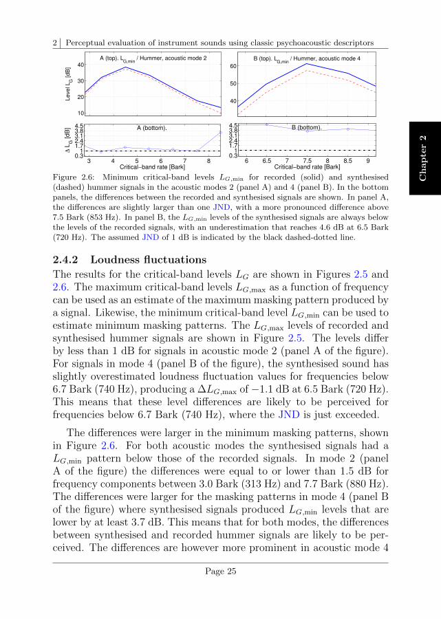
2 Perceptual evaluation of instrument sounds using classic psychoacoustic descriptors
Ch
ap
ter
2
10
20
30
40Level L
G [dB
]
A (top). LG,min
/ Hummer, acoustic mode 2
3 4 5 6 7 8
0.5
1
1.5
2
2.5
3
3.5
∆ L
G [dB
]
Critical−band rate [Bark]
A (bottom).
40
50
60
Level L
G [dB
]
B (top). LG,min
/ Hummer, acoustic mode 4
6 6.5 7 7.5 8 8.5 9
3.5
4
4.5
∆ L
G [dB
]
Critical−band rate [Bark]
B (bottom).
20
40
Level L
G [dB
]
A (top). LG,min
/ Hummer, acoustic mode 2
3 4 5 6 7 80.3
11.72.43.13.84.5
∆ L
G [dB
]
Critical−band rate [Bark]
A (bottom).
40
50
60
Level L
G [dB
]
B (top). LG,min
/ Hummer, acoustic mode 4
6 6.5 7 7.5 8 8.5 90.3
11.72.43.13.84.5
∆ L
G [dB
]
Critical−band rate [Bark]
B (bottom).
Figure 2.6: Minimum critical-band levels LG,min for recorded (solid) and synthesised(dashed) hummer signals in the acoustic modes 2 (panel A) and 4 (panel B). In the bottompanels, the differences between the recorded and synthesised signals are shown. In panel A,the differences are slightly larger than one JND, with a more pronounced difference above7.5 Bark (853 Hz). In panel B, the LG,min levels of the synthesised signals are always belowthe levels of the recorded signals, with an underestimation that reaches 4.6 dB at 6.5 Bark(720 Hz). The assumed JND of 1 dB is indicated by the black dashed-dotted line.
2.4.2 Loudness fluctuations
The results for the critical-band levels LG are shown in Figures 2.5 and2.6. The maximum critical-band levels LG,max as a function of frequencycan be used as an estimate of the maximum masking pattern produced bya signal. Likewise, the minimum critical-band level LG,min can be used toestimate minimum masking patterns. The LG,max levels of recorded andsynthesised hummer signals are shown in Figure 2.5. The levels differby less than 1 dB for signals in acoustic mode 2 (panel A of the figure).For signals in mode 4 (panel B of the figure), the synthesised sound hasslightly overestimated loudness fluctuation values for frequencies below6.7 Bark (740 Hz), producing a ∆LG,max of −1.1 dB at 6.5 Bark (720 Hz).This means that these level differences are likely to be perceived forfrequencies below 6.7 Bark (740 Hz), where the JND is just exceeded.
The differences were larger in the minimum masking patterns, shownin Figure 2.6. For both acoustic modes the synthesised signals had aLG,min pattern below those of the recorded signals. In mode 2 (panelA of the figure) the differences were equal to or lower than 1.5 dB forfrequency components between 3.0 Bark (313 Hz) and 7.7 Bark (880 Hz).The differences were larger for the masking patterns in mode 4 (panel Bof the figure) where synthesised signals produced LG,min levels that arelower by at least 3.7 dB. This means that for both modes, the differencesbetween synthesised and recorded hummer signals are likely to be per-ceived. The differences are however more prominent in acoustic mode 4
Page 25
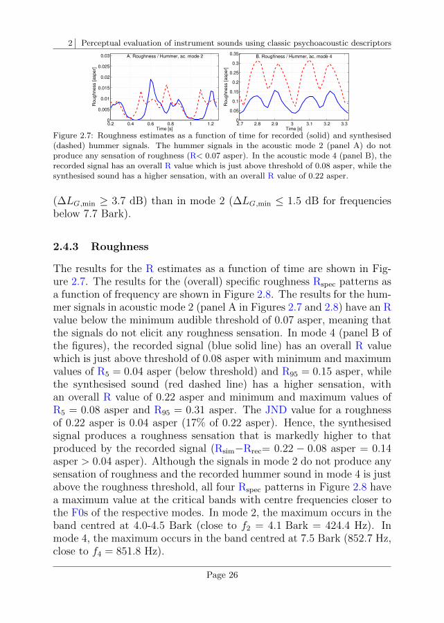
2 Perceptual evaluation of instrument sounds using classic psychoacoustic descriptors
0.2 0.4 0.6 0.8 1 1.20
0.005
0.01
0.015
0.02
0.025
0.03
Time [s]
Roughness [asper]
A. Roughness / Hummer, ac. mode 2
3 4 5 6 7 80
0.002
0.004
0.006
0.008
0.01
Critical−band rate [Bark]
Specific
roughness [asper/
Bark
]
A. Specific roughness / Hummer, ac. mode 2
2.7 2.8 2.9 3 3.1 3.2 3.30
0.05
0.1
0.15
0.2
0.25
0.3
0.35
Time [s]
Ro
ug
hn
ess [
asp
er]
B. Roughness / Hummer, ac. mode 4
6 7 8 9 100
0.02
0.04
0.06
0.08
0.1
Critical−band rate [Bark]
Sp
ecific
ro
ug
hn
ess [
asp
er/
Ba
rk]
B. Specific roughness / Hummer, ac. mode 4
Figure 2.7: Roughness estimates as a function of time for recorded (solid) and synthesised(dashed) hummer signals. The hummer signals in the acoustic mode 2 (panel A) do notproduce any sensation of roughness (R< 0.07 asper). In the acoustic mode 4 (panel B), therecorded signal has an overall R value which is just above threshold of 0.08 asper, while thesynthesised sound has a higher sensation, with an overall R value of 0.22 asper.
(∆LG,min ≥ 3.7 dB) than in mode 2 (∆LG,min ≤ 1.5 dB for frequenciesbelow 7.7 Bark).
2.4.3 Roughness
The results for the R estimates as a function of time are shown in Fig-ure 2.7. The results for the (overall) specific roughness Rspec patterns asa function of frequency are shown in Figure 2.8. The results for the hum-mer signals in acoustic mode 2 (panel A in Figures 2.7 and 2.8) have an Rvalue below the minimum audible threshold of 0.07 asper, meaning thatthe signals do not elicit any roughness sensation. In mode 4 (panel B ofthe figures), the recorded signal (blue solid line) has an overall R valuewhich is just above threshold of 0.08 asper with minimum and maximumvalues of R5 = 0.04 asper (below threshold) and R95 = 0.15 asper, whilethe synthesised sound (red dashed line) has a higher sensation, withan overall R value of 0.22 asper and minimum and maximum values ofR5 = 0.08 asper and R95 = 0.31 asper. The JND value for a roughnessof 0.22 asper is 0.04 asper (17% of 0.22 asper). Hence, the synthesisedsignal produces a roughness sensation that is markedly higher to thatproduced by the recorded signal (Rsim−Rrec= 0.22 − 0.08 asper = 0.14asper > 0.04 asper). Although the signals in mode 2 do not produce anysensation of roughness and the recorded hummer sound in mode 4 is justabove the roughness threshold, all four Rspec patterns in Figure 2.8 havea maximum value at the critical bands with centre frequencies closer tothe F0s of the respective modes. In mode 2, the maximum occurs in theband centred at 4.0-4.5 Bark (close to f2 = 4.1 Bark = 424.4 Hz). Inmode 4, the maximum occurs in the band centred at 7.5 Bark (852.7 Hz,close to f4 = 851.8 Hz).
Page 26

2 Perceptual evaluation of instrument sounds using classic psychoacoustic descriptors
Ch
ap
ter
2
0.2 0.4 0.6 0.8 1 1.20
0.005
0.01
0.015
0.02
0.025
0.03
Time [s]
Ro
ug
hn
ess [
asp
er]
A. Roughness / Hummer, ac. mode 2
3 4 5 6 7 80
0.002
0.004
0.006
0.008
0.01
Critical−band rate [Bark]
Sp
ecific
ro
ug
hn
ess [
asp
er/
Ba
rk]
A. Specific roughness / Hummer, ac. mode 2
2.7 2.8 2.9 3 3.1 3.2 3.30
0.05
0.1
0.15
0.2
0.25
0.3
0.35
Time [s]
Roughness [asper]
B. Roughness / Hummer, ac. mode 4
6 7 8 9 100
0.02
0.04
0.06
0.08
0.1
Critical−band rate [Bark]
Specific
roughness [asper/
Bark
]
B. Specific roughness / Hummer, ac. mode 4
Figure 2.8: Average specific roughness patterns Rspec for recorded (solid) and synthesised(dashed) hummer signals. All four Rspec patterns have a maximum value at the criticalbands with centre frequencies closer to the F0s of the respective modes. In acoustic mode 2(panel A), the maximum occurs in the band centred at 4.0-4.5 Bark (417.3-473.4 Hz, closeto f2 = 424.4 Hz). In acoustic mode 4 (panel B), the maximum occurs in the band centredat 7.5 Bark (852.7 Hz, close to f4 = 851.8 Hz).
3 4 5 6 7 8
0.04
0.08
0.12
0.16
Critical−band rate [Bark]
Specific
fi [
vacil/
Bark
]
A. Specific fluct. strength / Hummer, ac. mode 2
6 7 8 9 10
0.02
0.04
0.06
0.08
Critical−band rate [Bark]
Specific
fi [
vacil/
Bark
]
B. Specific fluct. strength / Hummer, ac. mode 4
Figure 2.9: Specific fluctuation strength pattern FSspec for recorded (solid) and synthesised(dashed) hummer signals. The overall FS values that can be obtained by integrating the areaunder the FSspec patterns are 0.18 and 0.29 vacil for the recorded and synthesised signals inacoustic mode 2, and 0.07 and 0.30 vacil in acoustic mode 4.
2.4.4 Fluctuation strength
The results for the patterns of specific fluctuation strength (FSspec) areshown in Figure 2.9. For this analysis, 2-s section of recorded and syn-thesised hummer sounds were used as input to the FS model. The anal-ysis window of the model was set to 2 s, meaning that the algorithmonly returned one overall FS value and one pattern of specific fluctu-ation strength FSspec. The overall FS values for recorded and synthe-sised signals in acoustic mode 2 were 0.18 vacil and 0.29 vacil, respec-tively. The FS values for the signals in acoustic mode 4 were 0.07 vaciland 0.30 vacil. In both modes the synthesised hummer signals elicit ahigher sensation of fluctuation than those of the recorded signals andthey differ by more than one JND. The JNDs for the FS values of0.29 and 0.30 vacil are about 0.03 vacil. Therefore, the differences areFSsim−FSrec= 0.29 − 0.18 = 0.11 vacil > 0.03 vacil in mode 2, andFSsim−FSrec= 0.30 − 0.07 = 0.23 vacil > 0.03 vacil in mode 4, i.e., inboth modes the differences in FS are larger than one JND. The FSvalue of the recorded hummer signal in the acoustic mode 4 is very low(0.07 vacil) and, therefore, it can be labelled as a non-fluctuating sound.
Page 27
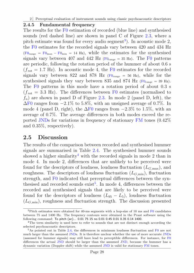
2 Perceptual evaluation of instrument sounds using classic psychoacoustic descriptors
2.4.5 Fundamental frequencyThe results for the F0 estimation of recorded (blue line) and synthesisedsounds (red dashed line) are shown in panel C of Figure 2.3, where apitch estimate was found for every audio segment3). In acoustic mode 2,the F0 estimates for the recorded signals vary between 420 and 434 Hz(F0range = F0max − F0min = 14 Hz), while the estimates for the synthesisedsignals vary between 407 and 442 Hz (F0range = 35 Hz). The F0 patternsare periodic, following the rotation period of the hummer of about 0.6 s(f rot = 1.7 Hz). In acoustic mode 4, the F0 estimates for the recordedsignals vary between 822 and 878 Hz (F0range = 56 Hz), while for thesynthesised signals they vary between 835 and 874 Hz (F0range = 39 Hz).The F0 patterns in this mode have a rotation period of about 0.3 s(f rot = 3.3 Hz). The differences between F0 estimates (normalised tofn) are shown in panel D of Figure 2.3. In mode 2 (panel D, left), the∆F0 ranges from −2.1% to 5.8%, with an unsigned average of 0.7%. Inmode 4 (panel D, right), the ∆F0 ranges from −2.3% to 1.5%, with anaverage of 0.7%. The average differences in both modes exceed the re-ported JNDs for variations in frequency of stationary FM tones (0.42%and 0.35%, respectively).
2.5 DiscussionThe results of the comparison between recorded and synthesised hummersignals are summarised in Table 2.4. The synthesised hummer soundsshowed a higher similarity4 with the recorded signals in mode 2 than inmode 4. In mode 2, differences that are unlikely to be perceived werefound for the descriptors of loudness, loudness fluctuation (LG,max), androughness. The descriptors of loudness fluctuation (LG,min), fluctuationstrength, and F0 indicated that perceptual differences between the syn-thesised and recorded sounds exist5. In mode 4, differences between therecorded and synthesised signals that are likely to be perceived werefound for the descriptors of loudness (L95 − L5), loudness fluctuation(LG,min), roughness and fluctuation strength. The discussion presented
3Pitch estimates were obtained for 40-ms segments with a hop-size of 10 ms and F0 candidatesbetween 75 and 1400 Hz. The frequency contours were obtained in the Praat software using thefollowing command: To pitch (ac)... 0.01 75 15 no 0.01 0.45 0.01 0.35 0.14 1400.
4The term similarity is used here to refer to sounds that are not distinct enough according theselected psychoacoustic descriptors.
5As pointed out in Table 2.4, the differences in minimum loudness fluctuation and F0 are notmuch larger than the assumed JNDs. It is therefore unclear whether the use of more accurate JNDs(assessed for hummer signals) may still have lead to perceptible differences. For instance, for F0differences the actual JND should be larger than the assumed JND, because the hummer has adynamic variation (Doppler shift) while the assumed JND is valid for stationary FM tones.
Page 28
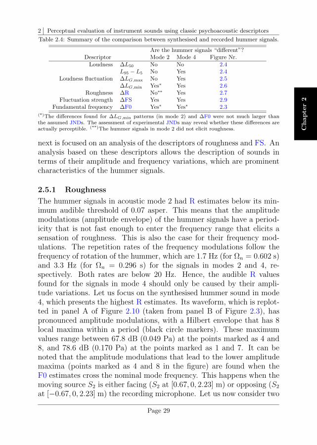
2 Perceptual evaluation of instrument sounds using classic psychoacoustic descriptors
Ch
ap
ter
2
Table 2.4: Summary of the comparison between synthesised and recorded hummer signals.
Are the hummer signals “different”?Descriptor Mode 2 Mode 4 Figure Nr.
Loudness ∆L50 No No 2.4L95 − L5 No Yes 2.4
Loudness fluctuation ∆LG,max No Yes 2.5∆LG,min Yes∗ Yes 2.6
Roughness ∆R No∗∗ Yes 2.7Fluctuation strength ∆FS Yes Yes 2.9
Fundamental frequency ∆F0 Yes∗ Yes∗ 2.3
(*)The differences found for ∆LG,min patterns (in mode 2) and ∆F0 were not much larger thanthe assumed JNDs. The assessment of experimental JNDs may reveal whether these differences areactually perceptible. (**)The hummer signals in mode 2 did not elicit roughness.
next is focused on an analysis of the descriptors of roughness and FS. Ananalysis based on these descriptors allows the description of sounds interms of their amplitude and frequency variations, which are prominentcharacteristics of the hummer signals.
2.5.1 Roughness
The hummer signals in acoustic mode 2 had R estimates below its min-imum audible threshold of 0.07 asper. This means that the amplitudemodulations (amplitude envelope) of the hummer signals have a period-icity that is not fast enough to enter the frequency range that elicits asensation of roughness. This is also the case for their frequency mod-ulations. The repetition rates of the frequency modulations follow thefrequency of rotation of the hummer, which are 1.7 Hz (for Ωn = 0.602 s)and 3.3 Hz (for Ωn = 0.296 s) for the signals in modes 2 and 4, re-spectively. Both rates are below 20 Hz. Hence, the audible R valuesfound for the signals in mode 4 should only be caused by their ampli-tude variations. Let us focus on the synthesised hummer sound in mode4, which presents the highest R estimates. Its waveform, which is replot-ted in panel A of Figure 2.10 (taken from panel B of Figure 2.3), haspronounced amplitude modulations, with a Hilbert envelope that has 8local maxima within a period (black circle markers). These maximumvalues range between 67.8 dB (0.049 Pa) at the points marked as 4 and8, and 78.6 dB (0.170 Pa) at the points marked as 1 and 7. It can benoted that the amplitude modulations that lead to the lower amplitudemaxima (points marked as 4 and 8 in the figure) are found when theF0 estimates cross the nominal mode frequency. This happens when themoving source S2 is either facing (S2 at [0.67, 0, 2.23] m) or opposing (S2
at [−0.67, 0, 2.23] m) the recording microphone. Let us now consider two
Page 29
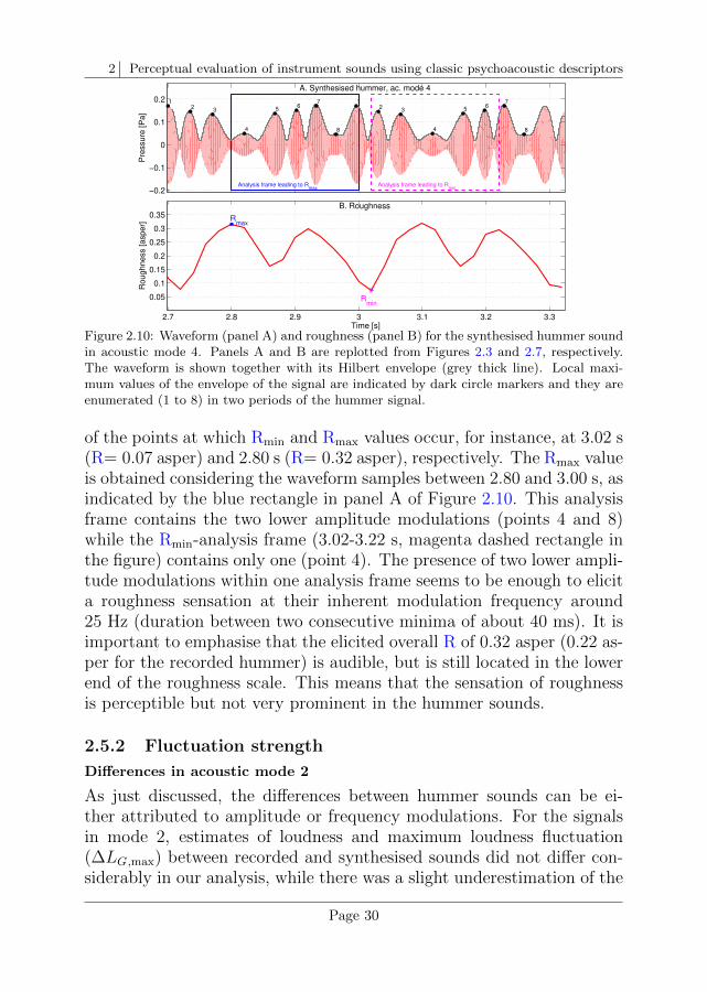
2 Perceptual evaluation of instrument sounds using classic psychoacoustic descriptors
−0.2
−0.1
0
0.1
0.2
Pre
ssure
[P
a]
A. Synthesised hummer, ac. mode 4
12
3
4
56
7
8
12
3
4
56
7
8
Analysis frame leading to Rmax
Analysis frame leading to Rmin
2.7 2.8 2.9 3 3.1 3.2 3.3
0.05
0.1
0.15
0.2
0.25
0.3
0.35 Rmax
Rmin
Time [s]
Roughness [asper]
B. Roughness
Figure 2.10: Waveform (panel A) and roughness (panel B) for the synthesised hummer soundin acoustic mode 4. Panels A and B are replotted from Figures 2.3 and 2.7, respectively.The waveform is shown together with its Hilbert envelope (grey thick line). Local maxi-mum values of the envelope of the signal are indicated by dark circle markers and they areenumerated (1 to 8) in two periods of the hummer signal.
of the points at which Rmin and Rmax values occur, for instance, at 3.02 s(R= 0.07 asper) and 2.80 s (R= 0.32 asper), respectively. The Rmax valueis obtained considering the waveform samples between 2.80 and 3.00 s, asindicated by the blue rectangle in panel A of Figure 2.10. This analysisframe contains the two lower amplitude modulations (points 4 and 8)while the Rmin-analysis frame (3.02-3.22 s, magenta dashed rectangle inthe figure) contains only one (point 4). The presence of two lower ampli-tude modulations within one analysis frame seems to be enough to elicita roughness sensation at their inherent modulation frequency around25 Hz (duration between two consecutive minima of about 40 ms). It isimportant to emphasise that the elicited overall R of 0.32 asper (0.22 as-per for the recorded hummer) is audible, but is still located in the lowerend of the roughness scale. This means that the sensation of roughnessis perceptible but not very prominent in the hummer sounds.
2.5.2 Fluctuation strength
Differences in acoustic mode 2
As just discussed, the differences between hummer sounds can be ei-ther attributed to amplitude or frequency modulations. For the signalsin mode 2, estimates of loudness and maximum loudness fluctuation(∆LG,max) between recorded and synthesised sounds did not differ con-siderably in our analysis, while there was a slight underestimation of the
Page 30
2 Perceptual evaluation of instrument sounds using classic psychoacoustic descriptors
Ch
ap
ter
2
minimum loudness fluctuation observed in the synthesised signal, withan overall ∆LG,min of −1.5 dB (0.5 dB beyond the assumed JND). If weuse loudness estimates as indicative of variations in the amplitude enve-lope, disregarding the 0.5-dB underestimation in LG,min, the differencein FS between hummer sounds should be caused by differences in theirfrequency modulations. The synthesised sound was found to have an F0with a larger variation (F0range) than that of the recorded sound (seeFigure 2.3, panel C, left). The F0 estimates have a periodicity relatedto the rotation frequency of the hummer, in this mode of f rot = 1.7 Hz(Ωn ≈ 0.6 s). Since this frequency lies within the range of frequenciesthat are relevant for fluctuation strength, we may attribute the higherFS of the synthesised signal to its more prominent Doppler shift (higherF0range value) with respect to the recorded signal.
Differences in acoustic mode 4
For the signals in mode 4, the descriptors of loudness and loudness fluc-tuations already showed an underestimation of the minimum amplitudevalues. This means that at least part of the difference (FSsim−FSrec=0.23 vacil) between FS values can be attributed to amplitude modula-tions. The recorded and synthesised hummer sounds were found to haveF0 ranges of 56 Hz (∆f ≈ ±28 Hz) and 39 Hz (∆f ≈ ±20 Hz), respec-tively. In an analysis presented in Appendix B, FM tones with a similarcarrier frequency (fc = 851.8 Hz), frequency deviation (∆±25 Hz), mod-ulation frequency (fmod= 4 Hz), and no amplitude modulation (flat enve-lope) elicited FS model estimates of 0.11 vacil or less. Since the frequencymodulations (FMs) follow a rotation frequency of f rot = 3.3 Hz (closeto fmod = 4 Hz), the analysis shown in the appendix can be used toargue that the difference between FS estimates in mode 4 is unlikely tobe produced by differences in the frequency modulation of the hummersounds.
2.6 Conclusions
The methods presented in this chapter have been applied to recordedand synthesised sounds of an instrument called hummer. The analysiswas based on five descriptors –loudness, loudness fluctuations, roughness,fluctuation strength, fundamental frequency–, that can be interpreted asan evaluation based on 5 dimensions. Within each of these dimensions,the psychoacoustic estimates obtained from the recorded and synthesisedsounds were considered as similar if they differed by less than one JND
Page 31
2 Perceptual evaluation of instrument sounds using classic psychoacoustic descriptors
and as perceptually different otherwise. The results showed that thesynthesised sounds are more similar to the recorded ones in acousticmode 2, where two of the descriptors differed by less than one JND(loudness and roughness) and one descriptor was just above the JND(loudness fluctuation), than in mode 4, where only one of the descriptorsmet such a criterion (loudness, L50).
The evaluated sounds are periodic and harmonic and they are char-acterised by the presence of both amplitude and frequency modulations.Based on these properties we assumed that the selected descriptors wereappropriate to evaluate differences between recorded and synthesisedhummer sounds. Other musical instruments may have properties thatrequire another set of descriptors, which can increase the difficulty ofthe evaluation if more descriptors are needed, requiring more knowledgeabout the underlying JNDs. Some other instrument properties may be:(1) the presence of temporal transients, and; (2) the transition in pitchpercepts from harmonic to non-harmonic segments within the sound.
In order to introduce the analysis of sounds that have temporal tran-sients, recorded piano sounds are studied in the next chapters (Chapters3, 4, 5). There, the perceptual similarity between sounds is approachedas an experimental (performance) task and it does not require an a prioriknowledge about the dimensions that are to be evaluated, as it was thecase in this chapter.
Page 32
3 Measuring the perceived similarity of instrumentsounds using an instrument-in-noise test
In this chapter the comparison between sounds is approached as a dis-crimination task. This discrimination task has been adapted to assess theperceptual similarity of two test sounds. In the previous chapter, twosounds were “judged” as very similar if a given psychoacoustic metricprovided values that differ by less than one JND. This situation wouldbe comparable to a listening condition of the same two sounds with alevel difference that is below the discriminability threshold.
In contrast to the use of a specific psychoacoustic metric, the proposedmethod is developed under the idea that, when comparing two sounds,a listener will use all available sound properties –or prominent features–rather than using a single property. The experiment is implemented asan “instrument”-in-noise task. The two sounds being evaluated are pre-sented with an added specific noise. By adjusting the SNR in the courseof the experiment the difficulty of the sound discrimination is manipu-lated. Two sounds that are similar will tolerate a low level of added noise(high SNR) to correctly discriminate one from the other in contrast tothe case of two sounds that are more dissimilar, where a higher amountof noise (lower SNR) will be tolerated before the discriminability perfor-mance decreases. In other words, a strong correlation between SNR andsimilarity is expected. To produce this effect, however, the noises needto have similar spectro-temporal properties to those of the test stimuli.For that purpose the algorithm of the ICRA noises in speech has beenadapted. A description to use this algorithm in the evaluation of a set oftest stimuli is given. As study case, the instrument-in-noise test is usedto evaluate recordings of one note played on seven Viennese pianos. Thesuggested method is compared to the method of triadic comparisons ina similarity assessment task.
Page 33
3 Measuring the perceived similarity between sounds using an instrument-in-noise test
3.1 Introduction
Perceptual similarity between elements is a problem approached in sev-eral disciplines and is normally assessed experimentally. Popular experi-mental tasks used to compare sounds are the method of triadic compar-isons (Levelt et al., 1966; Fritz et al., 2010; Novello et al., 2011), pair-wise comparisons (Grey, 1977; Grey & Gordon, 1978; Raake et al., 2014;Tahvanainen et al., 2015), free verbalisation rating, and categorisation(Dubois, 2000; Guastavino & Katz, 2004; Saitis et al., 2013). A reviewof these and other methods used in auditory research in the context ofmusical instruments is provided by Fritz and Dubois (2015) and also inthe introduction of this thesis (Section 1.3). For the methods of triadicand pairwise comparisons, matrices indicating the preferences of the par-ticipants can be constructed. To further process the data, the preferencematrices are normally converted into a mathematical space where theelements under test can be compared to each other. Techniques as MDS(Shepard, 1962; Kruskal, 1964b) and the use of the Bradley-Terry-Luce(BTL) scale (Bradley, 1953; Wickelmaier & Schmid, 2004) are examplesof algorithms that allow such a comparison.
Despite all those experimental procedures to evaluate similarity, ourinterest is not only on knowing which sounds are more or less similaramong each other but also on obtaining a quantifiable measure of thosedistances. In this chapter we show a way to reach that objective byconducting a listening test to discriminate two sounds using a 3-AFCexperiment in noise, where the noise allows to change the similarity ofthe sounds being tested. In the next section the discrimination test or“instrument”-in-noise test is explained, providing a detailed explanationof the noise generation. As study case, a comparison of one note (C#5) ofseven Viennese pianos from the 19th century is given. A description of themethod of triadic comparisons is also included. The triadic comparisontest is used as reference method in the validation of the instrument-in-noise task.
3.2 Description of the method
A method to quantify the perceptual differences between sounds is pre-sented in this section. The sounds are compared pairwise and they areembedded in a background noise at different SNRs. The method was de-veloped under the rationale that two very different sounds must be easyto discriminate while two similar sounds must represent a more difficult
Page 34
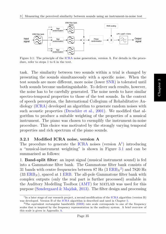
3 Measuring the perceived similarity between sounds using an instrument-in-noise test
Ch
ap
ter
3
Figure 3.1: The principle of the ICRA noise generation, version A. For details in the proce-dure, refer to steps 1 to 6 in the text.
task. The similarity between two sounds within a trial is changed bypresenting the sounds simultaneously with a specific noise. When thetest sounds are more different, more noise (lower SNR) is tolerated untilboth sounds become undistinguishable. To deliver such results, however,the noise has to be carefully generated. The noise needs to have similarspectro-temporal properties to those of the test sounds. In the contextof speech perception, the International Collegium of Rehabilitative Au-diology (ICRA) developed an algorithm to generate random noises withsuch acoustic properties (Dreschler et al., 2001). We modified that al-gorithm to produce a suitable weighting of the properties of a musicalinstrument. The piano was chosen to exemplify the instrument-in-noiseprocedure. This choice was motivated by the strongly varying temporalproperties and rich spectrum of the piano sounds.
3.2.1 Modified ICRA noise, version AThe procedure to generate the ICRA noises (version A1) introducinga “musical-instrument weighting” is shown in Figure 3.1 and can besummarised as follows:
1. Band-split filter: an input signal (musical instrument sound) is fedinto a Gammatone filter bank. The Gammatone filter bank consists of31 bands with centre frequencies between 87 Hz (3 ERBN
2) and 7820 Hz(33 ERBN), spaced at 1 ERB. The all-pole Gammatone filter bank withcomplex outputs (only the real part is further processed) available inthe Auditory Modelling Toolbox (AMT) for MATLAB was used for thispurpose (Søndergaard & Majdak, 2013). The filter design and processing
1In a later stage of our research project, a second modification of the ICRA algorithm (version B)was developed. Version B of the ICRA algorithm is described and used in Chapter 5.
2The equivalent rectangular bandwidth (ERB) rate scale corresponds to one of the frequencyscales that is inspired by the frequency representation in the auditory system. A brief overview ofthis scale is given in Appendix A.
Page 35
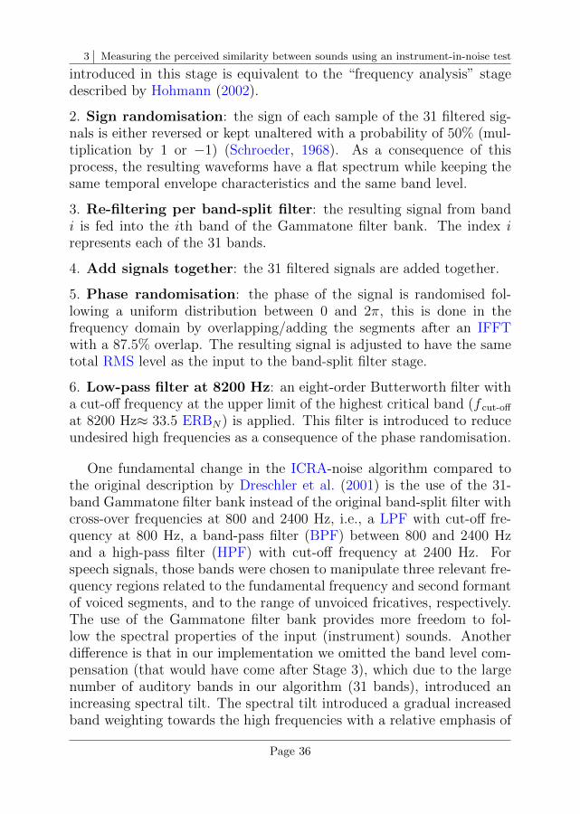
3 Measuring the perceived similarity between sounds using an instrument-in-noise test
introduced in this stage is equivalent to the “frequency analysis” stagedescribed by Hohmann (2002).
2. Sign randomisation: the sign of each sample of the 31 filtered sig-nals is either reversed or kept unaltered with a probability of 50% (mul-tiplication by 1 or −1) (Schroeder, 1968). As a consequence of thisprocess, the resulting waveforms have a flat spectrum while keeping thesame temporal envelope characteristics and the same band level.
3. Re-filtering per band-split filter: the resulting signal from bandi is fed into the ith band of the Gammatone filter bank. The index irepresents each of the 31 bands.
4. Add signals together: the 31 filtered signals are added together.
5. Phase randomisation: the phase of the signal is randomised fol-lowing a uniform distribution between 0 and 2π, this is done in thefrequency domain by overlapping/adding the segments after an IFFTwith a 87.5% overlap. The resulting signal is adjusted to have the sametotal RMS level as the input to the band-split filter stage.
6. Low-pass filter at 8200 Hz: an eight-order Butterworth filter witha cut-off frequency at the upper limit of the highest critical band (f cut-off
at 8200 Hz≈ 33.5 ERBN) is applied. This filter is introduced to reduceundesired high frequencies as a consequence of the phase randomisation.
One fundamental change in the ICRA-noise algorithm compared tothe original description by Dreschler et al. (2001) is the use of the 31-band Gammatone filter bank instead of the original band-split filter withcross-over frequencies at 800 and 2400 Hz, i.e., a LPF with cut-off fre-quency at 800 Hz, a band-pass filter (BPF) between 800 and 2400 Hzand a high-pass filter (HPF) with cut-off frequency at 2400 Hz. Forspeech signals, those bands were chosen to manipulate three relevant fre-quency regions related to the fundamental frequency and second formantof voiced segments, and to the range of unvoiced fricatives, respectively.The use of the Gammatone filter bank provides more freedom to fol-low the spectral properties of the input (instrument) sounds. Anotherdifference is that in our implementation we omitted the band level com-pensation (that would have come after Stage 3), which due to the largenumber of auditory bands in our algorithm (31 bands), introduced anincreasing spectral tilt. The spectral tilt introduced a gradual increasedband weighting towards the high frequencies with a relative emphasis of
Page 36
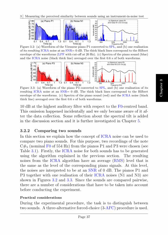
3 Measuring the perceived similarity between sounds using an instrument-in-noise test
Ch
ap
ter
3
0.1 0.4 0.7 1 1.3
50
55
60
65
70
75
80
Am
plit
ude [dB
SP
L]
Time [s]
(a) Piano P1
0.1 0.4 0.7 1 1.3Time [s]
(b) Noise N1
500 1000 2000 4000
25
30
35
40
45
50
55
60
65
70
Frequency [Hz]
Am
plit
ude [dB
]
(c) Spectrum: piano P1 and noise N1 (t=0−0.6 [s])
Figure 3.2: (a) Waveform of the Viennese piano P1 converted to SPL, and (b) one realisationof its resulting ICRA noise at an SNR= 0 dB. The thick black lines correspond to the Hilbertenvelope of the waveforms (LPF with cut-off at 20 Hz). (c) Spectra of the piano sound (blue)and the ICRA noise (black thick line) averaged over the first 0.6 s of both waveforms.
0.1 0.4 0.7 1 1.3
50
55
60
65
70
75
Am
plit
ud
e [
dB
SP
L]
Time [s]
(a) Piano P3
0.1 0.4 0.7 1 1.3Time [s]
(b) Noise N3
500 1000 2000 4000
20
25
30
35
40
45
50
55
60
65
Frequency [Hz]
Am
plit
ude [dB
]
(c) Spectrum: piano P3 and noise N3 (t=0−0.6 [s])
Figure 3.3: (a) Waveform of the piano P3 converted to SPL, and (b) one realisation of itsresulting ICRA noise at an SNR= 0 dB. The thick black lines correspond to the Hilbertenvelope of the waveforms. (c) Spectra of the piano sound (red) and the ICRA noise (blackthick line) averaged over the first 0.6 s of both waveforms.
10 dB at the highest auditory filter with respect to the F0-centred band.This omission happened incidentally and we only became aware of it af-ter the data collection. Some reflection about the spectral tilt is addedin the discussion section and it is further investigated in Chapter 5.
3.2.2 Comparing two sounds
In this section we explain how the concept of ICRA noise can be used tocompare two piano sounds. For this purpose, two recordings of the noteC#5 (nominal F0 of 554 Hz) from the pianos P1 and P3 were chosen (seeTable 3.1). Firstly, the ICRA noise for both sounds has to be generatedusing the algorithm explained in the previous section. The resultingnoises from the ICRA algorithm have an average (RMS) level that isthe same as the level of the corresponding piano signals. At this level,the noises are interpreted to be at an SNR of 0 dB. The pianos P1 andP3 together with one realisation of their ICRA noises (N1 and N3) areshown in Figures 3.2 and 3.3. Since the sounds are compared pairwise,there are a number of considerations that have to be taken into accountbefore conducting the experiment.
Practical considerations
During the experimental procedure, the task is to distinguish betweentwo sounds. A three-alternative forced-choice (3-AFC) procedure is used.
Page 37
3 Measuring the perceived similarity between sounds using an instrument-in-noise test
This procedure is also known as odd-ball paradigm. In this procedure,one of the two sounds serves as “reference” and is presented in two obser-vation intervals. The other sound serves as “test sound” and is presentedin the randomly chosen third interval.
The sounds being compared need to be of a similar duration. In theexample, both piano waveforms were set to have a duration of 1.3 s.Additionally the piano onset (leading to the maximum sound pressurelevel) was set to occur at approximately the same time stamp (t = 0.1 s).
The next consideration is to generate a “paired” ICRA noise that ac-counts for the spectro-temporal properties of both piano sounds. Thepaired noise is generated by combining the two ICRA noises (mean oftheir waveforms). The resulting noise is labelled as having an SNR of0 dB3. It is also assumed that the paired ICRA noise is efficient to grad-ually mask the properties of the test sounds when presented together (inthe example, P1 or P3 plus the paired noise) within each trial intervalas the noise level increases (and the SNR decreases). It is important,however, to use different realisations of the paired noise in every testinterval. This is because the use of a single fixed noise removes thestatistical variability of the masker and may introduce additional cuesduring the course of the experiment (von Klitzing & Kohlrausch, 1994).The use of a fixed noise is known as frozen noise. If additional decisioncues are available to the participant, the discrimination of the pianosbecomes easier. To avoid this problem, noises that are independentlygenerated but being drawn from the same statistical distribution areused. Such type of noises are known as running noises. To generate“running” ICRA noises, twelve realisations of each paired ICRA noisewere generated. Within each trial of the 3-AFC experiment three pairednoises are chosen, which leads to “12 choose 3” or
(123
)= 220 possible
triads of noises. If the selection of noises is randomly drawn from auniform distribution, it is unlikely that two participants use exactly thesame sequence of paired noises during the course of the experimentalsession. In order to perform the actual comparison between the pianosP1 and P3, the SNR of their paired ICRA noises is adapted by applyinga positive gain (decrease of the SNR, more difficult discrimination) or anegative gain (increase of the SNR, easier discrimination), depending onthe participant’s responses.
3By averaging the two waveforms the variance of the resulting paired noise is decreased by 3 dB.
Page 38
3 Measuring the perceived similarity between sounds using an instrument-in-noise test
Ch
ap
ter
3
3.2.3 Adaptive procedure: Instrument-in-noise testThe instrument sounds are compared pairwise. A given pair of soundsis presented in 3-AFC trials, where the discriminability threshold is es-timated by adjusting the noise level. This corresponds to an adaptiveprocedure (or staircase method). The participant has to indicate whichof the three intervals contains the target sound (presented once) wherethe reference sound is presented twice. The adjustable parameter (noiselevel) is varied following a two-down one-up rule: the noise is increased(SNR is decreased) after 2 consecutive right answers and decreased (SNRis increased) after 1 wrong answer. This paradigm tracks the 70.7%discriminability threshold (Levitt, 1971). Consecutive changes of theadaptive parameter in only one direction are “one run”. A down runrepresents consecutive changes of the noise towards more difficult condi-tions (decrease in SNR) while an up run is related to consecutive changestowards easier conditions (increase in SNR). Changes from down to up(correct to incorrect) or up to down (incorrect to correct), the reversals,are the relevant noise conditions used as criterion to stop the experimen-tal procedure. We chose to wait until 12 reversals are reached beforestopping the comparison between the test sounds. The starting point ofthe paired ICRA noise is set to an SNR of 16 dB. We assume that atthis SNR the discrimination of most piano pairs is easy and that this canhelp participants to get somehow accustomed to differences between thepianos being tested. The step size at which the noise is adjusted is set to4 dB and is reduced to 2 dB (after the 2nd reversal) and 1 dB (after the4th reversal). After the 4th reversal the runs stay at a fixed step size of1 dB. These runs correspond to the measuring stage. The median of thereversals during the measuring stage (last 8 reversals) is used to estimatethe discrimination threshold.
The sounds used in this chapter differ considerably in their loudnessdue to differences in the construction of the pianos from where theywere recorded, which was affected by the fast technological developmentsduring the 19th century. Loudness cues4 are, however, not the mainfocus of this research. To avoid the use of loudness cues during the
4Three technical aspects that influence the loudness of the piano sounds are: (1) Differences inthe force with which the hammer strikes the strings. One of the reasons for these differences is theuse of different types of hammer actions, as it is the case for pianos P5 and P6 (see Table 3.1);(2) Differences in the radiation pattern of the pianos. This is influenced by the soundboard design,which differs from piano to piano; (3) Differences in string-soundboard coupling. This can be due todifferences in both string and soundboard impedances at their coupling point. These three aspectsdo not only introduce loudness cues but also timbre (colour) cues. This means that despite thereduction of loudness cues in the experimental design, these aspects are at least partly present inthe sounds due to their influence on timbre.
Page 39
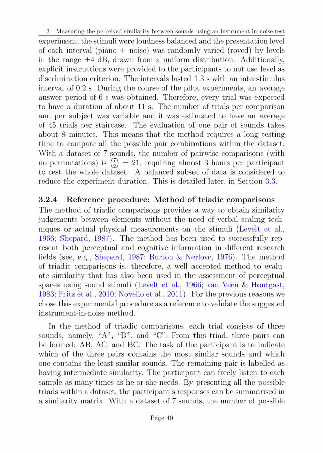
3 Measuring the perceived similarity between sounds using an instrument-in-noise test
experiment, the stimuli were loudness balanced and the presentation levelof each interval (piano + noise) was randomly varied (roved) by levelsin the range ±4 dB, drawn from a uniform distribution. Additionally,explicit instructions were provided to the participants to not use level asdiscrimination criterion. The intervals lasted 1.3 s with an interstimulusinterval of 0.2 s. During the course of the pilot experiments, an averageanswer period of 6 s was obtained. Therefore, every trial was expectedto have a duration of about 11 s. The number of trials per comparisonand per subject was variable and it was estimated to have an averageof 45 trials per staircase. The evaluation of one pair of sounds takesabout 8 minutes. This means that the method requires a long testingtime to compare all the possible pair combinations within the dataset.With a dataset of 7 sounds, the number of pairwise comparisons (withno permutations) is
(72
)= 21, requiring almost 3 hours per participant
to test the whole dataset. A balanced subset of data is considered toreduce the experiment duration. This is detailed later, in Section 3.3.
3.2.4 Reference procedure: Method of triadic comparisons
The method of triadic comparisons provides a way to obtain similarityjudgements between elements without the need of verbal scaling tech-niques or actual physical measurements on the stimuli (Levelt et al.,1966; Shepard, 1987). The method has been used to successfully rep-resent both perceptual and cognitive information in different researchfields (see, e.g., Shepard, 1987; Burton & Nerlove, 1976). The methodof triadic comparisons is, therefore, a well accepted method to evalu-ate similarity that has also been used in the assessment of perceptualspaces using sound stimuli (Levelt et al., 1966; van Veen & Houtgast,1983; Fritz et al., 2010; Novello et al., 2011). For the previous reasons wechose this experimental procedure as a reference to validate the suggestedinstrument-in-noise method.
In the method of triadic comparisons, each trial consists of threesounds, namely, “A”, “B”, and “C”. From this triad, three pairs canbe formed: AB, AC, and BC. The task of the participant is to indicatewhich of the three pairs contains the most similar sounds and whichone contains the least similar sounds. The remaining pair is labelled ashaving intermediate similarity. The participant can freely listen to eachsample as many times as he or she needs. By presenting all the possibletriads within a dataset, the participant’s responses can be summarised ina similarity matrix. With a dataset of 7 sounds, the number of possible
Page 40
3 Measuring the perceived similarity between sounds using an instrument-in-noise test
Ch
ap
ter
3
triads is(
73
)= 35. Within the 35 triads, each of the 21 possible piano
pairs is judged 5 times. The average time required to judge each trial,i.e., one triad, was 40 s meaning that a duration of about 23 minuteswas expected to evaluate the whole dataset once.
One method to further process the experimentally obtained similaritymatrix is the MDS algorithm (Shepard, 1962; Kruskal, 1964a, 1964b).MDS is commonly used as a visualisation tool of complex data. Thesimilarity matrix is an n×n matrix (7×7 if n = 7 elements). In the MDSalgorithm, the similarity matrix is assigned to a lower-dimensional space(n × q matrix), where the distance between elements is related to theperceptual similarity between them. The Euclidean distance between twoelements in the q-dimensional space is a reference for the discriminationthreshold estimated in the instrument-in-noise test.
3.3 Study case: Similarity among 19th-centuryViennese pianos
3.3.1 Stimuli
Recordings from seven pianos are compared among each other. The pi-anos were constructed in Vienna between 1805 and 1873. During thishistorical period, the piano construction underwent major developments.One important change during the 19th century was the increase of thestring tension at rest (by a factor of 4), with the purpose of increasingthe sound power of the piano. The soundboard, responsible for the soundradiation to the air, increased in thickness to withstand the higher stringtensions together with the inclusion of metallic parts after 1850. The ex-citation mechanism of the strings (the hammer) increased systematicallyits mass to increase the amplitude of the hammer impact (Chaigne etal., 2016; Chaigne, 2016). These changes affected the timbre (or colour)of the radiated piano sounds. We believe that these seven pianos are arepresentative sample of the timbre changes of the instrument.
Recordings of one note (C#5, F0 of 554 Hz) from the seven pianos wereused. One recording per piano was chosen leading to a total of 7 stimuli.The duration of each waveform was set to 1.3 s, with the note onsetoccurring at a time stamp of 0.1 s. The sounds were ramped down usinga 150-ms cosine ramp. The loudness of the sounds was adjusted to havea maximum value of 18 sone. For that purpose the short-term loudnessfrom the time-varying loudness (TVL) model (Glasberg & Moore, 2002)
Page 41

3 Measuring the perceived similarity between sounds using an instrument-in-noise test
Table 3.1: List of pianos used in the listening experiments. Information about the intensityof the sounds is shown. The loudness of the sounds when presented 4 dB softer and 4 dBharder are shown in parentheses.
Level [dB SPL] Loudness [sone]
ID / Year Manufacturer Lmax / Leq Smax / Savg
P1 / 1805∗ Gert Hecher 77.2 / 62.8 17.4 (13.7-22.0) / 6.8 (5.2-8.8)P2 / 1819 Nannette Streicher 74.9 / 58.8 17.2 (13.5-21.8) / 5.5 (4.2-7.2)P3 / 1828 Conrad Graf 73.7 / 55.4 17.0 (13.3-21.5) / 5.6 (4.3-7.3)P4 / 1836 Johann B. Streicher 83.7 / 66.3 18.5 (14.4-23.5) / 7.0 (5.3-9.1)P5 / 1851∗∗ Johann B. Streicher (English) 78.0 / 60.2 17.8 (14.1-22.4) / 6.6 (5.1-8.5)P6 / 1851∗∗ Johann B. Streicher (Viennese) 81.7 / 67.2 17.2 (13.5-21.8) / 7.3 (5.6-9.1)P7 / 1873 Johann B. Streicher & Sohn 81.7 / 67.2 17.4 (13.7-22.1) / 8.3 (6.3-10.7)
(*) Piano P1 is a contemporary replica of a piano built in 1805. (**) Pianos P5 and P6 differ in theirhammer action (English and Viennese, respectively).
was used. After the adjustment, the sounds had a maximum level rangingfrom 73.7 to 83.7 dB SPL (see Table 3.1).
In order to compensate for pitch differences in the piano recordings,the mean pitch of the sounds was adjusted to 554 Hz. The maximumpitch difference was for pianos P3 and P7 which had a mean pitch of519 Hz and no pitch adjustment was needed for the recording of PianoP6. The pitch adjustment was performed for each piano sound in twosteps. In step one, the pitch of the sound was scaled to the desired valueby using resampling. In step 2, a time stretch technique was used to keepthe duration of the pitch-adjusted sounds constant. The time stretch wasdone by using the phase vocoder algorithm (Ellis, 2002)5.
3.3.2 Apparatus
The experiments were conducted in a doubled-walled sound-proof booth.The stimuli were presented via Sennheiser HD 265 Linear circumauralheadphones in a diotic reproduction (identical left and right channels).The participant’s responses were collected on a computer using the soft-ware APEX (Francart et al., 2008) and the APE Toolbox for MATLAB
(De Man & Reiss, 2014) for the instrument-in-noise and the triadic com-parisons, respectively.
3.3.3 Participants
Twenty participants (8 females and 12 males) were recruited from theJF Schouten subject database of the TU/e university. At the time oftesting, the participants were between 19 and 38 years old (average of25) and they all had self-reported normal hearing. They provided their
5The phase vocoder algorithm is available at http://www.ee.columbia.edu/˜dpwe/resources/matlab/pvoc/ (Last accessed on 18/07/2018).
Page 42
3 Measuring the perceived similarity between sounds using an instrument-in-noise test
Ch
ap
ter
3
informed consent before starting the experimental session and were paidfor their contribution.
The sample size of 20 participants was assessed a priori aiming attesting the hypothesis that the data from the instrument-in-noise arehighly correlated (effect size or Pearson correlation of at least 0.6) withthe data from the triadic comparisons, with a power of 90%. This analy-sis was done in the software G*Power (Faul et al., 2007, 2009), requiring17 participants to reach the desired effect size. By increasing the numberof participants to 20 the observable effect size is reduced to 0.57.
3.3.4 Experimental sessions
The experimental sessions were organised in two one-hour sessions perparticipant, including breaks. For the instrument-in-noise test, each par-ticipant was asked to evaluate 11 piano pairs. This means that the wholedataset (21 piano pairs) is tested once every two participants, includingone common pair. For evaluating half of the dataset, a time of 1:30hours was estimated. For the triadic comparisons a duration of 24 min-utes was estimated. Participants were encouraged to take breaks if theyfelt tired or distracted, which may have resulted in longer and less ac-curate threshold estimations. The participants started the first sessionwith the evaluation of 17 randomly chosen triads. This served as a wayof familiarising the participants with the set of piano sounds. The ses-sion continued with 5 or 6 threshold estimations (staircase procedure)that always started at a low noise level (high SNR). Participants werenot allowed to repeat the trials and no feedback was provided about thecorrectness of their responses. During the second session the participantsevaluated the remaining 18 triads, followed by 6 or 5 threshold estima-tions, completing the total of 11 estimations. Two (or three) piano pairswere evaluated within the same experiment at a time, i.e., trials from2 (or 3) staircases were interleaved. This means that the participantdid not necessarily judge the same piano pair in consecutive trials. Forchoosing the distribution of piano pairs throughout the test, the order ofthe 21 pairs was randomised 5 times. Each randomisation was used toassign the piano combinations of 4 participants. Two participants testedthe same piano pairs but exchanging the test and reference sounds. Forinstance if the piano pair 57 (piano P7 being the reference sound) wasattributed to the one participant then the pair 75 (piano P5 being thereference sound) was attributed to the other participant. Two partici-pants tested the first 11 pairs of the randomisation and two participants
Page 43
3 Measuring the perceived similarity between sounds using an instrument-in-noise test
23 47 35 13 67 57 12 45 17 46 15 24 56 36 34 25 14 27 16 37 26
−6
−3
0
3
6
9
12
15
18
21
24
27
Piano pair
SN
R r
atio
at
thre
sh
old
[d
B]
Figure 3.4: Discrimination thresholds for the instrument-in-noise tests. The thresholds (redtriangles) are used as measure of similarity between the sounds and were assessed taking themedian across participants. The piano pairs are shown along the abscissa and are orderedfrom higher to lower SNR thresholds. The error bars represent IQRs.(*)The results for piano pair 47 consider 8 thresholds, with 3 estimations using the staircase procedureand 5 using a constant-stimulus procedure. See the text for further details.
tested the remaining 10 pairs of the randomisation plus one “commonpair” (total of 11 pairs). With this distribution method and after fin-ishing all the experimental sessions, each piano pair was tested 10 timeswith each piano sound in the pair being used 5 times as reference and5 times as test sound. For the common pairs (5 in total), two addi-tional comparisons were available, being evaluated 12 times. With thisconfiguration, the whole dataset was tested 10 times including 5 pairsthat were additionally tested twice. The expected number of estimationswas therefore 220.
3.4 Results
3.4.1 Instrument-in-noise testThe discrimination thresholds of the instrument-in-noise experiment areshown in Figure 3.4. The pooled thresholds were assessed by takingthe median of all individual threshold estimations per piano pair. Nodistinction was made between permuted piano pairs (e.g., pair 23 andpair 32 were pulled out together). The thresholds ranged from 20.75 dBfor pair 23 down to -1.75 dB for pair 26. The estimations had a largebetween-subject variability with a length of the IQRs from 19.0 dB (pair23) down to 3.25 dB (pair 57) with a median value of 8 dB. The results arebased on 179 staircase threshold estimations and 5 threshold estimationsusing a constant stimulus procedure. During the data collection 210of the 220 originally planned staircases were obtained. Ten thresholdswere not estimated: for pair 47 five staircases were not conducted being
Page 44

3 Measuring the perceived similarity between sounds using an instrument-in-noise test
Ch
ap
ter
3
5 10 15 20 25 30 35 40 45 50 550
2
4
6
8
10
12
14
16
Participant 4: Piano pair 45 SNR at threshold = 5.5 [dB] (std=4.5)
Trial Nr.
Adaptive p
ara
mete
r S
NR
[dB
]
Staircase
Reversals
Figure 3.5: Example of one of the staircases that was removed from the data analysis. In thiscase, the last 4 reversals (SNRs at around 2 dB) differ in more than 3 dB from the estimatedthreshold (SNR at 5.5 dB), that considered the last 8 reversals (filled circle markers).
replaced by results obtained from a constant stimulus procedure at anSNR of 20 dB, while for participant S14 five piano pairs were accidentallyskipped. For her, in session 1 and session 2 the same 6 pairs were tested.Only her results from session 1 were used in the data analysis. The resultsfrom session 2 were consistent and differed by no more than 2 dB withrespect to the thresholds obtained in session 1. From the 210 obtainedthreshold 31 estimations were excluded.
Exclusion criteria
Thirty-one staircases were excluded from the data analysis after the datacollection. Three staircases were incomplete, having less than 12 rever-sals. Three staircases were removed because the participants reached amaximum SNR of 50 dB (“minimum” noise level). This value was setin advance as floor condition. Participants reaching this point were notable at all to discriminate the two sounds being tested. The remaining25 thresholds were removed after a check of consistency of the staircases.For this the standard deviation of the reversals was assessed. Thresholdsestimations where the deviation of the reversals was larger than 3 dBwere removed. The removed thresholds were checked manually to con-firm that the staircase did indeed include inconsistencies between theconvergence point of the staircase and the estimated threshold. Sucha situation is illustrated in Figure 3.5 where one of those staircases isshown. This staircase has a convergence point (see the last four rever-sals) that differs from the threshold estimation by 3.5 dB.
Thresholds using a constant stimulus procedure
The evaluation of piano pair 47 (and 74) was for several participants verydifficult. As part of our hypotheses the discrimination of sounds at high
Page 45
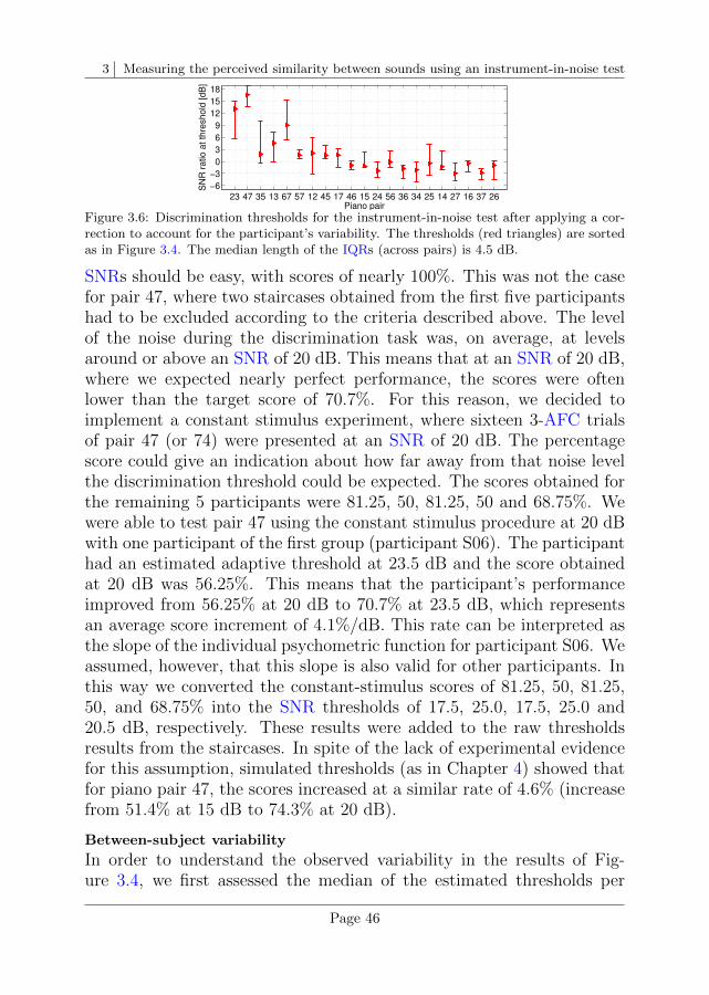
3 Measuring the perceived similarity between sounds using an instrument-in-noise test
23 47 35 13 67 57 12 45 17 46 15 24 56 36 34 25 14 27 16 37 26−6
−3
0
3
6
9
12
15
18
Piano pairS
NR
ra
tio
at
thre
sh
old
[d
B]
Figure 3.6: Discrimination thresholds for the instrument-in-noise test after applying a cor-rection to account for the participant’s variability. The thresholds (red triangles) are sortedas in Figure 3.4. The median length of the IQRs (across pairs) is 4.5 dB.
SNRs should be easy, with scores of nearly 100%. This was not the casefor pair 47, where two staircases obtained from the first five participantshad to be excluded according to the criteria described above. The levelof the noise during the discrimination task was, on average, at levelsaround or above an SNR of 20 dB. This means that at an SNR of 20 dB,where we expected nearly perfect performance, the scores were oftenlower than the target score of 70.7%. For this reason, we decided toimplement a constant stimulus experiment, where sixteen 3-AFC trialsof pair 47 (or 74) were presented at an SNR of 20 dB. The percentagescore could give an indication about how far away from that noise levelthe discrimination threshold could be expected. The scores obtained forthe remaining 5 participants were 81.25, 50, 81.25, 50 and 68.75%. Wewere able to test pair 47 using the constant stimulus procedure at 20 dBwith one participant of the first group (participant S06). The participanthad an estimated adaptive threshold at 23.5 dB and the score obtainedat 20 dB was 56.25%. This means that the participant’s performanceimproved from 56.25% at 20 dB to 70.7% at 23.5 dB, which representsan average score increment of 4.1%/dB. This rate can be interpreted asthe slope of the individual psychometric function for participant S06. Weassumed, however, that this slope is also valid for other participants. Inthis way we converted the constant-stimulus scores of 81.25, 50, 81.25,50, and 68.75% into the SNR thresholds of 17.5, 25.0, 17.5, 25.0 and20.5 dB, respectively. These results were added to the raw thresholdsresults from the staircases. In spite of the lack of experimental evidencefor this assumption, simulated thresholds (as in Chapter 4) showed thatfor piano pair 47, the scores increased at a similar rate of 4.6% (increasefrom 51.4% at 15 dB to 74.3% at 20 dB).
Between-subject variability
In order to understand the observed variability in the results of Fig-ure 3.4, we first assessed the median of the estimated thresholds per
Page 46

3 Measuring the perceived similarity between sounds using an instrument-in-noise test
Ch
ap
ter
3
participant. Since the difficulty in the judgement of the piano pairsshould be distributed across the 11 pairs evaluated per participant, themedian thresholds give an indication about how sensitive each partici-pant was during the course of the experiments. A lower median thresholdindicates more sensitivity and, correspondingly, a higher threshold indi-cates less sensitivity to the cues available in the piano waveforms. Thelowest and highest median SNR thresholds were found for participantsS14 (avg. SNR=−7.25 dB) and S10 (avg. SNR=18.5 dB), with a me-dian SNR across participants of 4.0 dB. This supports the existence ofa strong difference in the participant’s sensitivity. The SNR thresholdsafter a correction factor is applied are shown in Figure 3.6. The cor-rection depends on the median participant thresholds. For instance, forthe thresholds of participants S14 and S10 a correction of +7.25 and−18.5 dB (additive inverse values) was applied. With the correction themedian length of the IQRs decreased from 8.0 to 4.5 dB. Although sev-eral piano pairs changed their rank order (the thresholds in Figure 3.6are not monotonically decreasing), the rank-order correlation indicate astrong relationship of rs(19) = 0.83, p < 0.0016, between the thresholdsbefore and after being corrected. This small effect is caused becausethe correction moved the pairs around but only in neighbouring rela-tive locations. Despite the fact that with the results shown in Figure3.6 the between-subject variability is almost halved, they are not usedfor any further processing in this chapter. We assume that the choiceof the median as measure of central tendency of the thresholds is ro-bust enough to deal with the large IQRs and that the results withoutcorrection (Figure 3.4) are representative.
3.4.2 Triadic comparison
The results of all participants were pulled out to construct the similaritymatrix shown in the upper right triangle of Table 3.2. All participantsjudged the whole dataset of 35 possible triads once. Within the 35 tri-ads the 21 pairs were judged 5 times. These numbers are relevant tounderstand the range of possible scores in the similarity matrix.
Construction of the similarity matrix
The similarity matrix is a way to summarise how often each piano pairwas chosen as most similar, most dissimilar or indirectly chosen as havingan intermediate similarity, when presented in triads with the other test
6The value between brackets indicate the degrees of freedom, which is N − 2, with N being thenumber of data points being compared.
Page 47
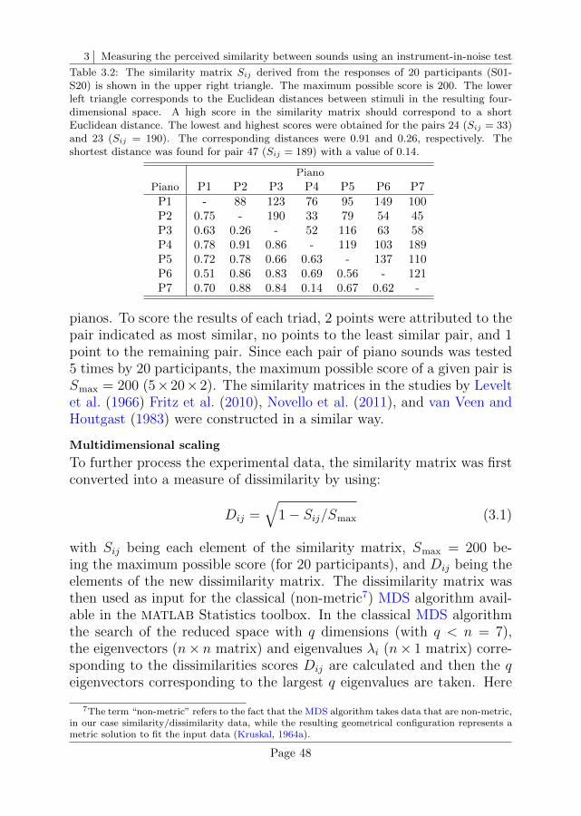
3 Measuring the perceived similarity between sounds using an instrument-in-noise test
Table 3.2: The similarity matrix Sij derived from the responses of 20 participants (S01-S20) is shown in the upper right triangle. The maximum possible score is 200. The lowerleft triangle corresponds to the Euclidean distances between stimuli in the resulting four-dimensional space. A high score in the similarity matrix should correspond to a shortEuclidean distance. The lowest and highest scores were obtained for the pairs 24 (Sij = 33)and 23 (Sij = 190). The corresponding distances were 0.91 and 0.26, respectively. Theshortest distance was found for pair 47 (Sij = 189) with a value of 0.14.
Piano
Piano P1 P2 P3 P4 P5 P6 P7P1 - 88 123 76 95 149 100P2 0.75 - 190 33 79 54 45P3 0.63 0.26 - 52 116 63 58P4 0.78 0.91 0.86 - 119 103 189P5 0.72 0.78 0.66 0.63 - 137 110P6 0.51 0.86 0.83 0.69 0.56 - 121P7 0.70 0.88 0.84 0.14 0.67 0.62 -
pianos. To score the results of each triad, 2 points were attributed to thepair indicated as most similar, no points to the least similar pair, and 1point to the remaining pair. Since each pair of piano sounds was tested5 times by 20 participants, the maximum possible score of a given pair isSmax = 200 (5×20×2). The similarity matrices in the studies by Leveltet al. (1966) Fritz et al. (2010), Novello et al. (2011), and van Veen andHoutgast (1983) were constructed in a similar way.
Multidimensional scaling
To further process the experimental data, the similarity matrix was firstconverted into a measure of dissimilarity by using:
Dij =√
1− Sij/Smax (3.1)
with Sij being each element of the similarity matrix, Smax = 200 be-ing the maximum possible score (for 20 participants), and Dij being theelements of the new dissimilarity matrix. The dissimilarity matrix wasthen used as input for the classical (non-metric7) MDS algorithm avail-able in the MATLAB Statistics toolbox. In the classical MDS algorithmthe search of the reduced space with q dimensions (with q < n = 7),the eigenvectors (n× n matrix) and eigenvalues λi (n× 1 matrix) corre-sponding to the dissimilarities scores Dij are calculated and then the qeigenvectors corresponding to the largest q eigenvalues are taken. Here
7The term “non-metric” refers to the fact that the MDS algorithm takes data that are non-metric,in our case similarity/dissimilarity data, while the resulting geometrical configuration represents ametric solution to fit the input data (Kruskal, 1964a).
Page 48
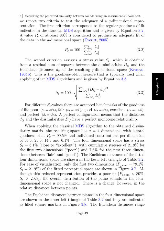
3 Measuring the perceived similarity between sounds using an instrument-in-noise test
Ch
ap
ter
3
we report two criteria to test the adequacy of a q-dimensional repre-sentation. The first criterion corresponds to the regular goodness-of-fitindicator in the classical MDS algorithm and is given by Equation 3.2.A value Pq of at least 80% is considered to produce an adequate fit ofthe data in the q-dimensional space (Everitt, 2005).
Pq = 100 ·∑q
i=1 |λi|∑ni=1 |λi|
(3.2)
The second criterion assesses a stress value St, which is obtainedfrom a residual sum of squares between the dissimilarities Dij and theEuclidean distances dij of the resulting q-dimensional space (Kruskal,1964b). This is the goodness-of-fit measure that is typically used whenapplying other MDS algorithms and is given by Equation 3.3.
St = 100 ·
√√√√∑i<j (Dij − dij)2∑i<j D
2ij
(3.3)
For different St-values there are accepted benchmarks of the goodnessof fit: poor (St = 20%), fair (St = 10%), good (St = 5%), excellent (St = 2.5%),and perfect (St = 0%). A perfect configuration means that the distancesdij and the dissimilarities Dij have a perfect monotone relationship.
When applying the classical MDS algorithm to the obtained dissim-ilarity matrix, the resulting space has q = 4 dimensions, with a totalgoodness of fit Pq = 99.5% and individual contributions per dimensionof 53.5, 25.6, 14.3 and 6.1%. The four dimensional space has a stressSt = 3.1% (close to “excellent”), with cumulative stresses of 21.9% forthe first two dimensions (“poor”) and 7.5% for the first three dimen-sions (between “fair” and “good”). The Euclidean distances of the fittedfour-dimensional space are shown in the lower left triangle of Table 3.2.For ease of visualisation, only the first two dimensions (Pq ,cum = 79.1%,St = 21.9%) of the fitted perceptual space are shown in Figure 3.7. Al-though this reduced representation provides a poor fit (Pq ,cum < 80%;St > 20%), the overall distribution of the piano sounds in the four-dimensional space is not changed. There is a change, however, in therelative distances between points.
The Euclidean distances between pianos in the four-dimensional spaceare shown in the lower left triangle of Table 3.2 and they are indicatedas filled square markers in Figure 3.8. The Euclidean distances range
Page 49

3 Measuring the perceived similarity between sounds using an instrument-in-noise test
−0.4 −0.2 0 0.2 0.4 0.6
−0.4
−0.2
0
0.2
0.4
0.6
1
23
4
5
6
7
Dimension 1
Dim
en
sio
n 2
Figure 3.7: Perceptual space obtained with the classical MDS algorithm. Only the first two(out of four) dimensions are shown. This space suggests that the piano sounds (note C#5)can be classified into four groups: pianos 16, 23, 47, and piano P5. Although the goodness offit of this reduced representation is poor (Pq ,cum = 79.1%; St = 21.9%) the overall distri-bution of the pianos in the space is not changed in the four dimensional space. The greybubbles give an indication of the participant’s variability: the bigger the bubble the higherthe variability across participants. Note that the axes of the MDS space are not to scale.
between 0.14 (for pair 47) and 0.91 (for pair 24) with approximately 50%of the distances lying in the range between dij ,25 =0.63 and dij ,75 =0.83.
The results shown in Figure 3.7 suggest that the pianos (so far, lim-ited to the note C#5) can be classified into four distinct groups: pianosP1+P6, pianos P2+P3, pianos P4+P7 and piano P5. Although pianoP5 seems to have an intermediate similarity with all these groups, in thefour-dimensional space its distances increase systematically. The dis-tances for all the other pianos do not differ considerably with respect tothe ones in the two-dimensional representation.
Between-subject variability
The classical MDS algorithm does not provide any indication of the vari-ability across participants in the resulting fitted space. One solution tothis problem is provided by the individual differences scaling algorithm(INDSCAL) (Carroll & Chang, 1970). Within INDSCAL an individualperceptual space is assessed for every participant. Those spaces are as-sumed to be a weighted version of the resulting perceptual space, withdifferent weights for different participants. With this approach it is pos-sible to assess the stress of each stimulus per participant, which can beused for obtaining measures of variability. Although the data were pro-cessed using INDSCAL as implemented by de Leeuw and Mair (2009),this algorithm was finally not used because the fitted pooled space vio-lated the condition of monotonicity between the Dij and dij. An alter-native approach was used that follows a similar idea to operate with the
Page 50
3 Measuring the perceived similarity between sounds using an instrument-in-noise test
Ch
ap
ter
3
23 47 35 13 67 57 12 45 17 46 15 24 56 36 34 25 14 27 16 37 26
0.1
0.2
0.3
0.4
0.5
0.6
0.7
0.8
0.9
Eu
clid
ea
n d
ista
nce
Piano pair
Figure 3.8: Euclidean distances taken from the four-dimensional perceptual space. Thesedistances are also shown in the lower left triangle of Table 3.2. The piano pairs are sorted inthe same way as in Figure 3.4. For a perfect consistency between these Euclidean distancesand the instrument-in-noise results, the distances should increase monotonically. This doesnot happen but the correlation between distances and SNR thresholds are moderate tohigh, with values of −0.47 (Pearson) and −0.64 (Spearman) (see Figure 3.9). The errorbars indicate the minimum and maximum distances between piano pairs across the 5 four-dimensional spaces assessed with data subsets every 4 participants.
stresses. Having as reference the fitted four-dimensional space, 5 dissim-ilarity matrices were generated pulling out the data of the participantsS01-S04, S05-S08, S09-S12, S13-S16, and S17-S20, respectively. The clas-sical MDS algorithm was applied, obtaining 5 new coordinates for eachof the 7 test pianos. For each of the 7 pianos, the distances between these5 coordinates and the coordinates in the pooled four-dimensional spacewas obtained, storing the difference between the minimum and maxi-mum distances. Half of that difference is used as radius of the “bubbles”in Figure 3.7. The diameter of the bubbles has a median of 0.15, rang-ing from 0.06 (piano P4) to 0.29 (piano P5), which can be interpretedas piano P4 being judged more consistently across participants and pi-ano P5 being scored more differently, leading to a higher between-subjectvariability. The obtained 5 four-dimensional spaces were used to assessthe minimum and maximum distances between piano pairs and they areshown as error bars in Figure 3.8. Those deviations range between 0.05(pair 57) and 0.33 (pair 16), with a median length of 0.17.
3.5 Discussion
A high perceptual similarity is equivalent to a high SNR threshold anda short Euclidean distance. If the results of both methods are con-sistent, the SNR thresholds of Figure 3.4, that are sorted in decreas-ing order, should correspond to monotonically increasing Euclidean dis-
Page 51
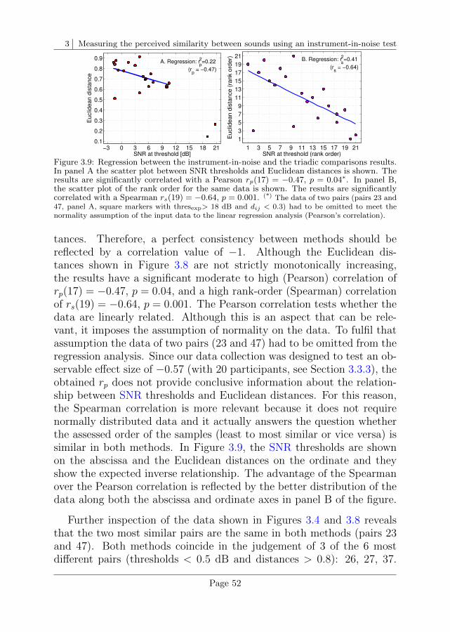
3 Measuring the perceived similarity between sounds using an instrument-in-noise test
−3 0 3 6 9 12 15 18 210.1
0.2
0.3
0.4
0.5
0.6
0.7
0.8
0.9
SNR at threshold [dB]
Euclid
ean d
ista
nce
Regression analysis − Pearson
A. Regression: rp
2=0.22
(rp = −0.47)
1 3 5 7 9 11 13 15 17 19 21
1
3
5
7
9
11
13
15
17
19
21
SNR at threshold (rank order)
Eu
clid
ea
n d
ista
nce
(ra
nk o
rde
r)
Regression analysis − Spearman
B. Regression: rs
2=0.41
(rs = −0.64)
Figure 3.9: Regression between the instrument-in-noise and the triadic comparisons results.In panel A the scatter plot between SNR thresholds and Euclidean distances is shown. Theresults are significantly correlated with a Pearson rp(17) = −0.47, p = 0.04∗. In panel B,the scatter plot of the rank order for the same data is shown. The results are significantlycorrelated with a Spearman rs(19) = −0.64, p = 0.001. (*) The data of two pairs (pairs 23 and47, panel A, square markers with thresexp> 18 dB and dij < 0.3) had to be omitted to meet thenormality assumption of the input data to the linear regression analysis (Pearson’s correlation).
tances. Therefore, a perfect consistency between methods should bereflected by a correlation value of −1. Although the Euclidean dis-tances shown in Figure 3.8 are not strictly monotonically increasing,the results have a significant moderate to high (Pearson) correlation ofrp(17) = −0.47, p = 0.04, and a high rank-order (Spearman) correlationof rs(19) = −0.64, p = 0.001. The Pearson correlation tests whether thedata are linearly related. Although this is an aspect that can be rele-vant, it imposes the assumption of normality on the data. To fulfil thatassumption the data of two pairs (23 and 47) had to be omitted from theregression analysis. Since our data collection was designed to test an ob-servable effect size of −0.57 (with 20 participants, see Section 3.3.3), theobtained rp does not provide conclusive information about the relation-ship between SNR thresholds and Euclidean distances. For this reason,the Spearman correlation is more relevant because it does not requirenormally distributed data and it actually answers the question whetherthe assessed order of the samples (least to most similar or vice versa) issimilar in both methods. In Figure 3.9, the SNR thresholds are shownon the abscissa and the Euclidean distances on the ordinate and theyshow the expected inverse relationship. The advantage of the Spearmanover the Pearson correlation is reflected by the better distribution of thedata along both the abscissa and ordinate axes in panel B of the figure.
Further inspection of the data shown in Figures 3.4 and 3.8 revealsthat the two most similar pairs are the same in both methods (pairs 23and 47). Both methods coincide in the judgement of 3 of the 6 mostdifferent pairs (thresholds < 0.5 dB and distances > 0.8): 26, 27, 37.
Page 52
3 Measuring the perceived similarity between sounds using an instrument-in-noise test
Ch
ap
ter
3
Piano P5 has an intermediate similarity with all the other pianos, withEuclidean distances between 0.56 (pair 56) and 0.78 (pair 15), this meansthat 5 (out of 6) distances are within the IQR of the distance data(dij,25−75 = 0.63 − 0.83). This is also supported by the results of theinstrument-in-noise test, where 5 (out of 6) thresholds lie within theIQR (SNR25−75 = 0.2−7.7 dB). For two pairs (16 and 56), both methodsprovide very different similarity measures. In both cases, the pairs arejudged as being more similar in the triadic comparisons.
Although we hypothesised that the ICRA noises follow the spectro-temporal properties of the input piano sounds, as pointed out in Sec-tion 3.2.1, our algorithm “version A” introduced an incidental spectralmismatch that is gradual towards high frequencies. The effect of thisspectral tilt is investigated in Chapter 5 and is compared with an up-dated version of the ICRA algorithm, “version B”.
3.6 ConclusionIn this chapter we have presented a method to conduct a within-instru-ment comparison, measuring the perceptual similarity among test soundsusing an instrument-in-noise test. In this method, the noise is matchedto the spectro-temporal properties of the pair of sounds being tested.
Similarity among 19th-century Viennese pianos
As a study case, a comparison among recordings of one note (C#5)played on Viennese pianos from the 19th century was shown. The re-sults of the instrument-in-noise test were compared with the results ofthe method of triadic comparisons, which is a method commonly usedto map a set of stimuli into a perceptual similarity space. The resultsof both methods, collected from 20 participants, had a high and signif-icant rank-order (Spearman) correlation of rs(19) = −0.64, p = 0.001.The correlation results denote a high inverse relationship between SNRthresholds and Euclidean distances, meaning that a higher thresholdresults in a lower Euclidean distance. The results obtained from theinstrument-in-noise method are consistent with overall subjective simi-larity judgements. Therefore, the instrument-in-noise procedure seemsto be a promising method to quantify perceptual differences betweensounds.
What is different when using the instrument-in-noise method?
It was pointed out that the instrument-in-noise method is rather timeconsuming when compared to the method of triadic comparisons (about
Page 53
3 Measuring the perceived similarity between sounds using an instrument-in-noise test
7 times slower), so why to choose it then? Despite the longer testingtime, one of the advantages of the instrument-in-noise method is thatit allows to measure similarity by evaluating different test conditions(different SNRs) where the physical properties of the test sounds are af-fected. This approach can be seen as a quantifiable way to manipulatethe similarity between test sounds. On the contrary, the triadic com-parisons are conducted at a fixed test condition (in our case in silence,i.e., at a very high SNR) and that leads (after data processing) to apurely psychological space where the physical properties of the soundsare kept constant. With this argument, the instrument-in-noise test cangive an indication not only of which samples are closer or farther apartfrom each other (psychological approach), but can also provide evidenceabout their acoustic properties at noise levels below (SNRs above) andat threshold (physical approach).
Extending the use of the instrument-in-noise method
The key point of the instrument-in-noise method is the use of a noisethat is shaped in spectral and temporal properties to the test sounds.The ICRA algorithm (Dreschler et al., 2001), used originally to generatespeech maskers, was adapted to provide a suitable solution for instrumentsounds. The described instrument-in-noise method can be used not onlyin the evaluation of other piano notes but also to evaluate any otherinstrument, as far as some practical aspects regarding the stimuli arefollowed. For the piano sounds, some of these aspects were: to have teststimuli with the same pitch, similar durations, a piano onset occurringat a “synchronised” time stamp, and to balance for any cue that is notdesired to be judged (we kept the maximum loudness constant acrossstimuli). Some of the cues that were available to our participants were theenvelope, attack and decay of the waveforms and their spectral content.
For the evaluation of other piano notes or other musical instruments,the ICRA noises have to be generated again in order to match thespectro-temporal properties of the “new” test sounds.
Page 54
4 Simulating the perceived similarity ofinstrument sounds using an auditory model
In this chapter an auditory model which predicts psychoacoustic data isapplied to the problem of perceptual similarity between complex sounds.The perceptual similarity task corresponds to the instrument-in-noisetest presented and validated in Chapter 3. The same set of loudness-balanced piano sounds is used here.
The concept of similarity can be studied as a sensory process but, asargued in the next section, also as a cognitive process. The auditorymodel used in this chapter accounts primarily for the first aspect andalso includes a “memory” stage that can be interpreted as a cognitivecomponent within the model. The challenge of this chapter is the ad-justment of the memory stage of the auditory model, i.e., the assessmentand use of the so-called template of the system, in order to extend its useto account for the human performance in a similarity task using complex(piano) sounds.
4.1 Introduction
In the context of acoustics, similarity assessments are used in soundquality evaluation (see, e.g., Hansen & Kollmeier, 2000; Kates & Arehart,2014) and in the study of specific sound types (see, e.g., Grey, 1977;Fritz et al., 2010). The study case of Chapter 2 is another exampleof this latter use. The concept of similarity is relevant because in aneveryday listening experience, (sound) objects are unlikely to be repeatedin exactly the same way (see, e.g., Shepard, 1987). Therefore, there issome acquired familiarisation used to recall those similar (sound) objects.For this reason, the concept of similarity has been studied as a cognitiveor top-down process, reflecting the familiarisation with the object, aswell as a perceptual or sensory process, reflecting how a given stimuluscan “match” that object. In this chapter we use an auditory model
Page 55
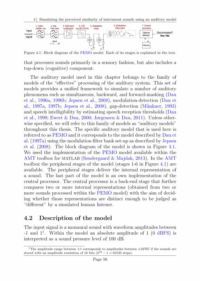
4 Simulating the perceived similarity of instrument sounds using an auditory model
Figure 4.1: Block diagram of the PEMO model. Each of its stages is explained in the text.
that processes sounds primarily in a sensory fashion, but also includes atop-down (cognitive) component.
The auditory model used in this chapter belongs to the family ofmodels of the “effective” processing of the auditory system. This set ofmodels provides a unified framework to simulate a number of auditoryphenomena such as simultaneous, backward, and forward-masking (Dauet al., 1996a, 1996b; Jepsen et al., 2008), modulation-detection (Dau etal., 1997a, 1997b; Jepsen et al., 2008), gap-detection (Munkner, 1993)and speech intelligibility by estimating speech reception thresholds (Dauet al., 1999; Ewert & Dau, 2000; Jørgensen & Dau, 2011). Unless other-wise specified, we will refer to this family of models as “auditory models”throughout this thesis. The specific auditory model that is used here isreferred to as PEMO and it corresponds to the model described by Dau etal. (1997a) using the modulation filter bank set-up as described by Jepsenet al. (2008). The block diagram of the model is shown in Figure 4.1.We used the implementation of the PEMO model available within theAMT toolbox for MATLAB (Søndergaard & Majdak, 2013). In the AMTtoolbox the peripheral stages of the model (stages 1-6 in Figure 4.1) areavailable. The peripheral stages deliver the internal representation ofa sound. The last part of the model is an own implementation of thecentral processor. The central processor is a back-end stage that furthercompares two or more internal representations (obtained from two ormore sounds processed within the PEMO model) with the aim of decid-ing whether those representations are distinct enough to be judged as“different” by a simulated human listener.
4.2 Description of the model
The input signal is a monaural sound with waveform amplitudes between-1 and 11. Within the model an absolute amplitude of 1 (0 dBFS) isinterpreted as a sound pressure level of 100 dB.
1The amplitude range between ±1 corresponds to amplitudes between ±32767 if the sounds arestored with an amplitude resolution of 16 bits (216 − 1 = 65535 steps).
Page 56
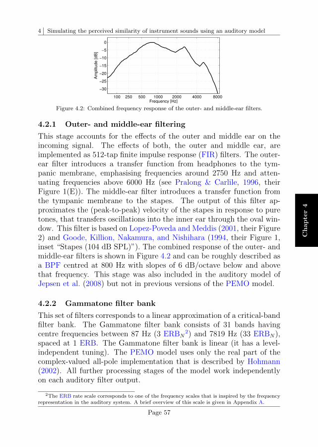
4 Simulating the perceived similarity of instrument sounds using an auditory model
Ch
ap
ter
4
100 250 500 1000 2000 4000 8000
−30
−25
−20
−15
−10
−5
0
Frequency [Hz]
Am
plit
ude [dB
]
Figure 4.2: Combined frequency response of the outer- and middle-ear filters.
4.2.1 Outer- and middle-ear filtering
This stage accounts for the effects of the outer and middle ear on theincoming signal. The effects of both, the outer and middle ear, areimplemented as 512-tap finite impulse response (FIR) filters. The outer-ear filter introduces a transfer function from headphones to the tym-panic membrane, emphasising frequencies around 2750 Hz and atten-uating frequencies above 6000 Hz (see Pralong & Carlile, 1996, theirFigure 1(E)). The middle-ear filter introduces a transfer function fromthe tympanic membrane to the stapes. The output of this filter ap-proximates the (peak-to-peak) velocity of the stapes in response to puretones, that transfers oscillations into the inner ear through the oval win-dow. This filter is based on Lopez-Poveda and Meddis (2001, their Figure2) and Goode, Killion, Nakamura, and Nishihara (1994, their Figure 1,inset “Stapes (104 dB SPL)”). The combined response of the outer- andmiddle-ear filters is shown in Figure 4.2 and can be roughly described asa BPF centred at 800 Hz with slopes of 6 dB/octave below and abovethat frequency. This stage was also included in the auditory model ofJepsen et al. (2008) but not in previous versions of the PEMO model.
4.2.2 Gammatone filter bank
This set of filters corresponds to a linear approximation of a critical-bandfilter bank. The Gammatone filter bank consists of 31 bands havingcentre frequencies between 87 Hz (3 ERBN
2) and 7819 Hz (33 ERBN),spaced at 1 ERB. The Gammatone filter bank is linear (it has a level-independent tuning). The PEMO model uses only the real part of thecomplex-valued all-pole implementation that is described by Hohmann(2002). All further processing stages of the model work independentlyon each auditory filter output.
2The ERB rate scale corresponds to one of the frequency scales that is inspired by the frequencyrepresentation in the auditory system. A brief overview of this scale is given in Appendix A.
Page 57
4 Simulating the perceived similarity of instrument sounds using an auditory model
4.2.3 Hair-cell transduction
This stage accounts for the inner hair-cell processing. It simulates thetransformation from mechanical oscillations in the basilar membrane intoreceptor potentials in the inner hair cells. The signals are first half-waverectified and then low-pass filtered using 5 first-order infinite impulseresponse (IIR) filters with a cut-off frequency of 2000 Hz. The half-waverectification keeps the positive part of the signal. The combined effectof the cascade of LPFs is equivalent to applying a fifth-order IIR filterwith cut-off frequency of 770 Hz. With this LPF, the frequency compo-nents below 770 Hz are almost unaffected, so that the phase informationis kept (a maximum attenuation of 3 dB is reached when approaching770 Hz), frequency components between 770 Hz and 2000 Hz are grad-ually attenuated (attenuations between 3 dB at 770 Hz down to 15 dBat 2000 Hz), meaning that the phase information is gradually lost. Forfrequency components above 2000 Hz almost all the phase informationis removed (more than 15 dB of attenuation, slope of −30 dB/octave).This way of removing phase information is consistent with the decreaseof phase locking observed in the auditory nerve (Breebaart et al., 2001).
4.2.4 Adaptation
This stage simulates the adaptive properties of the auditory system at thelevel of the auditory nerve (see, e.g., Kohlrausch et al., 1992). Adaptationrefers to changes in the gain of the system when the level of the inputsignal changes. When a change in the signal level is “rapid”, the gain ofthe system remains constant and the level is transformed linearly. Forslower variations, the signal level is compressed. This adaptation stageis implemented as 5 feedback loops, each of them having a different timeconstant (τ = 5, 50, 129, 253, 500 ms). In this study an overshoot limitationis used, meaning that the output value for rapid input changes (relativeto the time constants) is limited to a maximum value of 5 times thestationary output value for the same level. The limiter factor limit= 5differs with respect to the usual limiter factor of 10 used in the auditorymodels (Munkner, 1993; Dau et al., 1997a). Due to the relevance ofthe note onset in piano sounds, the choice of this new limiter factor is asensitive parameter which strongly influenced the simulation results thatare shown later in this chapter. The effect of using the new limiter factoron the resulting internal representations is described in the next section.The interested reader is also referred to Appendix C, where an in-depthreview of the properties of the adaptation loops is given.
Page 58
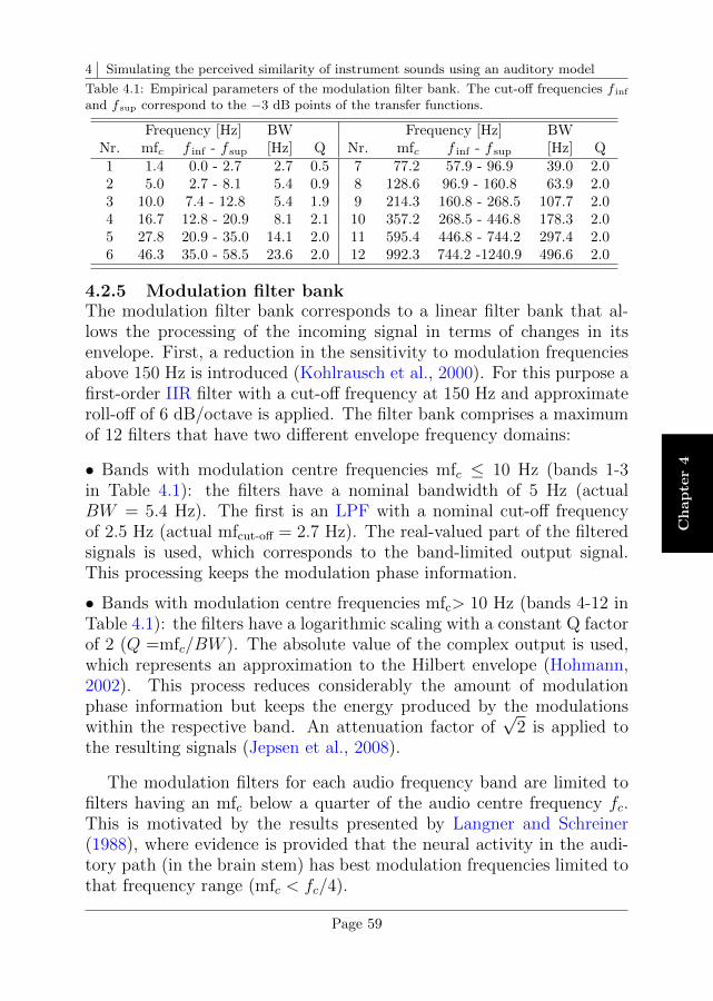
4 Simulating the perceived similarity of instrument sounds using an auditory model
Ch
ap
ter
4
Table 4.1: Empirical parameters of the modulation filter bank. The cut-off frequencies f inf
and f sup correspond to the −3 dB points of the transfer functions.
Frequency [Hz] BW Frequency [Hz] BWNr. mfc f inf - f sup [Hz] Q Nr. mfc f inf - f sup [Hz] Q1 1.4 0.0 - 2.7 2.7 0.5 7 77.2 57.9 - 96.9 39.0 2.02 5.0 2.7 - 8.1 5.4 0.9 8 128.6 96.9 - 160.8 63.9 2.03 10.0 7.4 - 12.8 5.4 1.9 9 214.3 160.8 - 268.5 107.7 2.04 16.7 12.8 - 20.9 8.1 2.1 10 357.2 268.5 - 446.8 178.3 2.05 27.8 20.9 - 35.0 14.1 2.0 11 595.4 446.8 - 744.2 297.4 2.06 46.3 35.0 - 58.5 23.6 2.0 12 992.3 744.2 -1240.9 496.6 2.0
4.2.5 Modulation filter bankThe modulation filter bank corresponds to a linear filter bank that al-lows the processing of the incoming signal in terms of changes in itsenvelope. First, a reduction in the sensitivity to modulation frequenciesabove 150 Hz is introduced (Kohlrausch et al., 2000). For this purpose afirst-order IIR filter with a cut-off frequency at 150 Hz and approximateroll-off of 6 dB/octave is applied. The filter bank comprises a maximumof 12 filters that have two different envelope frequency domains:
• Bands with modulation centre frequencies mfc ≤ 10 Hz (bands 1-3in Table 4.1): the filters have a nominal bandwidth of 5 Hz (actualBW = 5.4 Hz). The first is an LPF with a nominal cut-off frequencyof 2.5 Hz (actual mfcut-off = 2.7 Hz). The real-valued part of the filteredsignals is used, which corresponds to the band-limited output signal.This processing keeps the modulation phase information.
• Bands with modulation centre frequencies mfc> 10 Hz (bands 4-12 inTable 4.1): the filters have a logarithmic scaling with a constant Q factorof 2 (Q =mfc/BW ). The absolute value of the complex output is used,which represents an approximation to the Hilbert envelope (Hohmann,2002). This process reduces considerably the amount of modulationphase information but keeps the energy produced by the modulationswithin the respective band. An attenuation factor of
√2 is applied to
the resulting signals (Jepsen et al., 2008).
The modulation filters for each audio frequency band are limited tofilters having an mfc below a quarter of the audio centre frequency fc.This is motivated by the results presented by Langner and Schreiner(1988), where evidence is provided that the neural activity in the audi-tory path (in the brain stem) has best modulation frequencies limited tothat frequency range (mfc < fc/4).
Page 59
4 Simulating the perceived similarity of instrument sounds using an auditory model
4.2.6 Central processorIn this stage, the information received from the modulation filter bankis compared with a reference representation or “sound image” that isstored in the “memory” of the model. Inspired by the concept of anoptimal detector, borrowed from signal detection theory (see, e.g., Green& Swets, 1966, their chapters 6 and 7), the model can be seen as anartificial listener3 and the “memory” of the model can be seen as anexpected sound representation, learned by experience, that gives a clearindication to the artificial listener about “what to listen for” (Green &Swets, 1966; Dau et al., 1996a). This memory is referred to as template.
In a 3-AFC task, there are three intervals that can be compared withthe template. If the representations of each interval are labelled as Rx
with x = 1, 2, 3, the interval having the highest similarity with the tem-plate would be always chosen by the artificial listener. One mathematicalway to express this idea is to assess the cross-correlation value (CCV)between the representation Rx and the template Tp:
CCVx =1
fs
N∑n=1
Rx[n] · Tp[n] (4.1)
It is important to stress that the template Tp is a unit energy represen-tation while the representation Rx is not. As explained in subsequentsections, however, a difference representation ∆Rx is used in this equa-tion instead of the direct use of the representation Rx.
Memory: Use of a template
The use of a memory template, or simply template, assumes that in thedetection of a signal (or object) among other signals (or objects), sometype of awareness about the target signal is used. This corresponds toa top-down process and can be seen as a cognitive component in theauditory model. This approach is also used in the field of vision wherethere is evidence of brain activity in response to features of the expectedsignal (see, e.g., Chelazzi et al., 1993). The template is derived or, inother words, is “learned” by the artificial listener, at the beginning ofthe experiment simulation in a condition that is assumed to be easilydetected (low-noise condition, high SNR). This condition is referred toas a suprathreshold SNR. In the simulations, the suprathreshold SNRwas set to 21 dB. This condition is 5 dB higher in SNR (lower noise)than the initial SNR of the experimental sessions.
3In the literature (and in this thesis), the terms “artificial listener” and “artificial observer” areused interchangeably.
Page 60
4 Simulating the perceived similarity of instrument sounds using an auditory model
Ch
ap
ter
4
Template in a similarity task
The derivation of the template Tp in a similarity task where two soundsare compared is determined by: (a) the two test sounds, the target and“reference”, and; (b) two or more realisations of a noise that can effi-ciently mask the properties of both piano sounds. To account for thelatter aspect, ICRA noises (in this chapter using version A of the al-gorithm, as in Chapter 3) are used in every piano presentation. Forthe first aspect, the internal representations of both, the target pianoRt(MT ) and reference piano Rr(MT ) have to be used, because theirdiscrimination threshold depends on how different they are from eachother. The argument (MT ) indicates that the derivation of Tp shouldbe done at a highly discriminable noise level, that is, at a low noise level(high SNR). In the course of this research different ways of derivingthe template Tp using Rt(MT ) and Rr(MT ) were evaluated. Except forthe adopted approach which is described in this section, the alternativeapproaches are described in Appendix E.
In the adopted approach, two templates are derived: (a) Tp,t for thetarget piano sound, and (b) Tp,r for the reference piano sound. Foreach of the templates, an average representation of the piano soundsembedded in four different realisations of the ICRA noises at a highlydiscriminable condition (here at an SNR of 21 dB) is obtained4. Theaverage representations are normalised to unit energy. In this way, thetemplates satisfy (see also Equation E.3, in Appendix E):
Et =1
fs
N∑n=1
T 2p,t[n] = 1
Er =1
fs
N∑n=1
T 2p,r[n] = 1 (4.2)
where N corresponds to the number of samples used by the artificiallistener to make the decision. If the artificial listener uses the wholepiano waveforms, then N is defined by the total length of the sounds(1.3 s for the anechoic pianos)5. A longer “observation” (listening) periodwould mean that the listener makes use of the undershoot effect after
4The number of ICRA noise realisations (four) used to derive each average piano-plus-noiserepresentation was an arbitrary choice.
5In analogy to the theory of optimal detectors presented by Green and Swets (1966), wetreat the templates Tp,t and Tp,r as “expected signals” along one (temporal) dimension. Infact, there are two other dimensions: audio and modulation frequency. Considering all tem-plate dimensions and following the nomenclature of Equation 4.7, Equation 4.2 would turn intoEt = 1
fs
∑Mm=1
∑Kk=1
∑Nn=1 T
2p,t mk[n] = 1.
Page 61

4 Simulating the perceived similarity of instrument sounds using an auditory model
the piano sounds vanish. Based on our experimental design, where thepiano intervals had an interstimulus time of 0.2 s, the maximum possibleobservation period is 1.5 s. The results in the subsequent sections show,however, that an actual observation period of 0.5 s or less provides abetter fit between simulated and experimental thresholds than the useof full piano waveforms.
Use of two templates
In the course of the simulation of a 3-AFC task the “expected signals”or templates (Tp,t and Tp,r) have to be compared with the intervals (x =1, 2, 3) of each trial. The expression shown in Equation 4.1 is used forthis purpose but using a difference representation ∆Rx instead of thedirect use of the representation Rx. The representation ∆Rx is obtainedas the difference between the “piano-plus-noise” representation Rx andthe representation of the corresponding paired ICRA noise RN,x at theSNR of the ongoing trial, obtaining three ∆Rx representations6.
Due to the use of two templates, six CCV values are obtained, withthree CCV values corresponding to the comparison between each (dif-ference) interval representation ∆Rx with the target template Tp,t andthree corresponding to the comparison with the reference template Tp,r:
CCVx,t =1
fs
N∑n=1
∆Rx[n] · Tp,t[n]
CCVx,r =1
fs
N∑n=1
∆Rx[n] · Tp,r[n] with x = 1, 2, 3 (4.3)
Based on these six CCV values, the artificial listener chooses the intervalthat is more likely to contain the target sound using two criteria. Ifwe assume that the target interval is presented in the first observationinterval, then for a correct discrimination:
max
CCVx,t
= CCV1,t
min
CCVx,r
= CCV1,r with x = 1, 2, 3 (4.4)
6The use of difference representations ∆Rx is relevant for our decision approach due to the useof two templates. Since the unit energy normalisation of the templates is done independently, thenoise alone representations RN,x that are used in both criteria will always have different CCVx,t
and CCVx,r values. Subtracting the noise alone representations in the CCV calculation implies thatthe resulting CCVx,t and CCVx,r values correspond to the contribution of information of piano xrelative to the contribution of the noise x.
Page 62
4 Simulating the perceived similarity of instrument sounds using an auditory model
Ch
ap
ter
4
In other words, the target template Tp,t is expected to elicit the maximumCCV value when being correlated with the target interval. Likewise, thereference template Tp,r elicits higher CCV values when being correlatedwith the reference intervals and therefore the lowest CCV value is at-tributed to the target interval. The hat symbol indicates that the CCVvalues differ from the exact definition given in Equation 4.3. This iscaused by an internal noise, whose values are drawn from a Gaussian dis-tribution N(µ, σ2) with mean µ = 0 and standard deviation σ = 10.1 MU(variance of σ2). In our implementation of the internal noise, three num-bers are added to the corresponding CCVx value:
CCVx,t = CCVx,t +Nx(µ, σ2)
CCVx,r = CCVx,r +Nx(µ, σ2) with x = 1, 2, 3 (4.5)
Since µ = 0, the standard deviation σ corresponds to the actual sourceof internal variability in the decision process. The use of this Gaussiannoise leads to a reduction in the process performance when either theCCVx,t values get close to each other or when the CCVx,r values do. Thestandard deviation σ = 10.1 Model Units (MU) was obtained by runningan increment-discrimination task with each piano sound and trackingthe amount of noise needed to produce an average performance of 70.7%for a difference in level of ∆L = 1 dB. This procedure is described inAppendix D.
Compensating the misalignment between piano representations
One final aspect in the decision criterion is that the cross-correlationbetween the templates and the interval representations should deliverthe highest CCV values. As described in Section 3.3.1, the piano stim-uli are aligned to have the note onset at a time stamp of 0.1 s. Thisalignment criterion seemed to be enough to perceive each of the pianosounds aligned with the ICRA noise within each piano-plus-noise inter-val. However, this does not always ensure a maximum CCV value duringthe decision process. This is particularly sensitive when correlating ei-ther the target piano representation with the reference template Tp,r orthe reference piano representation with the target template Tp,t. Duringthe simulations, the cross-correlation function is assessed for each inter-val, with time lags between −50 ms and 50 ms (in steps of 1 ms). Themaximum of the cross-correlation function is used as the CCVx value forthe decision stage (Equation 4.5).
Page 63
4 Simulating the perceived similarity of instrument sounds using an auditory model
4.2.7 Sources of internal and external variabilityThe processing of sounds in the auditory system is influenced by un-certainties in the stimuli and by internal variability caused, e.g., by im-perfections in memory and changes in the level of concentration (see,e.g., Yost et al., 1989). In this thesis we differentiate between sources ofvariability that are internal or external. Uncertainties in the stimuli arerelated to an external source of variability, while the effects of humanmemory and concentration correspond to sources of internal variability.To (partly) account for variations in human performance due to sourcesof internal variability, an internal noise is often used within computa-tional frameworks of auditory processing. In our model implementation,the internal noise is simulated by adding a Gaussian noise N(µ, σ2) withmean µ = 0 and standard deviation σ = 10.1 MU (see Equation 4.5and Appendix D). In threshold-detection tasks a typical source of ex-ternal variability is the use of running noise. Running noise refers tothe fact that in different intervals of a trial, different realisations of simi-larly generated noises are used. In the instrument-in-noise test a runningnoise condition is approximated by using 12 different ICRA noise reali-sations for each piano pair. Another source of external variability in theinstrument-in-noise test is the presentation level of each interval, whichis randomised (roved) by levels in the range ±4 dB.
4.3 Description of internal representations
4.3.1 General description of the representationsThe internal representation of pianos P1 and P3 after the last stageof peripheral processing of the auditory model (stage 6, modulation fil-ter bank) is shown in Figure 4.3. The analysis is shown for one audiofrequency band (centred at fc = 11 ERBN or 520 Hz, closest band toF0= 554 Hz). The piano sounds start at t = 0.1 s and their onsets oc-cur shortly thereafter. The onset of the lowest modulation filter (Nr. 1,mfc = 1.4 Hz) occurs approximately at t = 0.20 s, for filter Nr. 2 att = 0.15 s and for the rest of the filters between t =0.10 and t =0.11 s.In the figure, it can also be observed that after the piano onset, the am-plitudes in the modulation filters of P3 (Nr. 2-8) present more variationsin comparison with piano P1, especially for t = 1.0− 1.3 s.
We next describe the effect of using a stronger limiter factor in theadaptation loop stage. For this analysis the initial part (first 0.25 s ofthe waveform) of one of the piano sounds (piano P1) is further described.This description is also valid for the other 6 piano sounds of the dataset.
Page 64
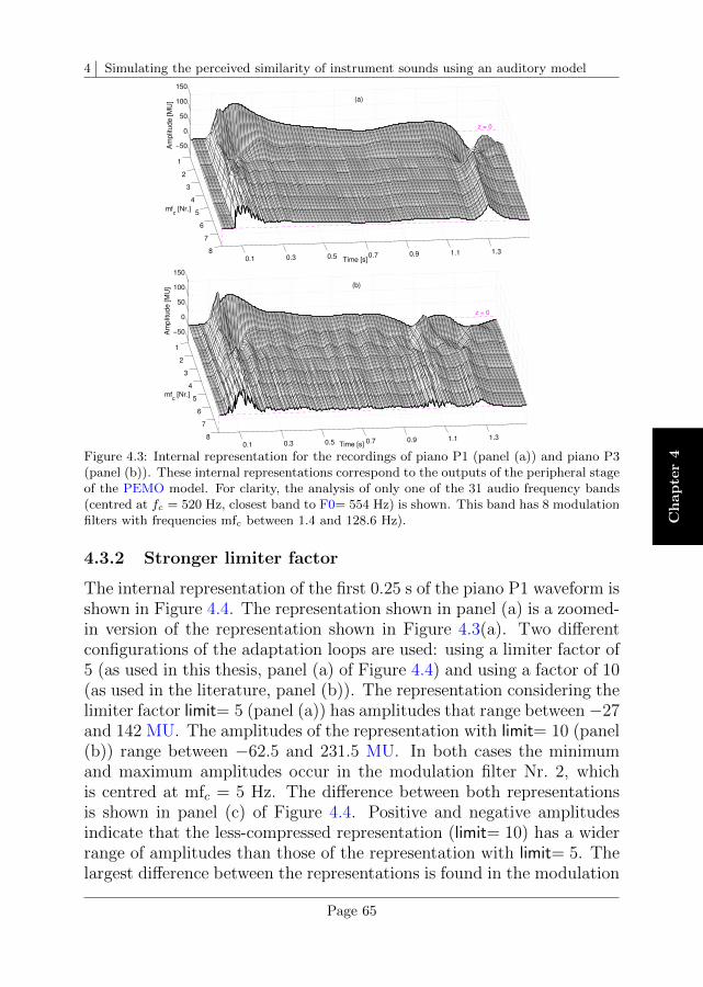
4 Simulating the perceived similarity of instrument sounds using an auditory model
Ch
ap
ter
4
0.1 0.3 0.5 0.7 0.9 1.1 1.38
7
6
5
4
3
2
1
−50
0
50
100
150
z = 0
(a)
Time [s]
mfc [Nr.]
Am
plit
ude [M
U]
0.1 0.3 0.5 0.7 0.9 1.1 1.38
7
6
5
4
3
2
1
−50
0
50
100
150
z = 0
(b)
Time [s]
mfc [Nr.]
Am
plit
ude [M
U]
Figure 4.3: Internal representation for the recordings of piano P1 (panel (a)) and piano P3(panel (b)). These internal representations correspond to the outputs of the peripheral stageof the PEMO model. For clarity, the analysis of only one of the 31 audio frequency bands(centred at fc = 520 Hz, closest band to F0= 554 Hz) is shown. This band has 8 modulationfilters with frequencies mfc between 1.4 and 128.6 Hz).
4.3.2 Stronger limiter factor
The internal representation of the first 0.25 s of the piano P1 waveform isshown in Figure 4.4. The representation shown in panel (a) is a zoomed-in version of the representation shown in Figure 4.3(a). Two differentconfigurations of the adaptation loops are used: using a limiter factor of5 (as used in this thesis, panel (a) of Figure 4.4) and using a factor of 10(as used in the literature, panel (b)). The representation considering thelimiter factor limit= 5 (panel (a)) has amplitudes that range between−27and 142 MU. The amplitudes of the representation with limit= 10 (panel(b)) range between −62.5 and 231.5 MU. In both cases the minimumand maximum amplitudes occur in the modulation filter Nr. 2, whichis centred at mfc = 5 Hz. The difference between both representationsis shown in panel (c) of Figure 4.4. Positive and negative amplitudesindicate that the less-compressed representation (limit= 10) has a widerrange of amplitudes than those of the representation with limit= 5. Thelargest difference between the representations is found in the modulation
Page 65
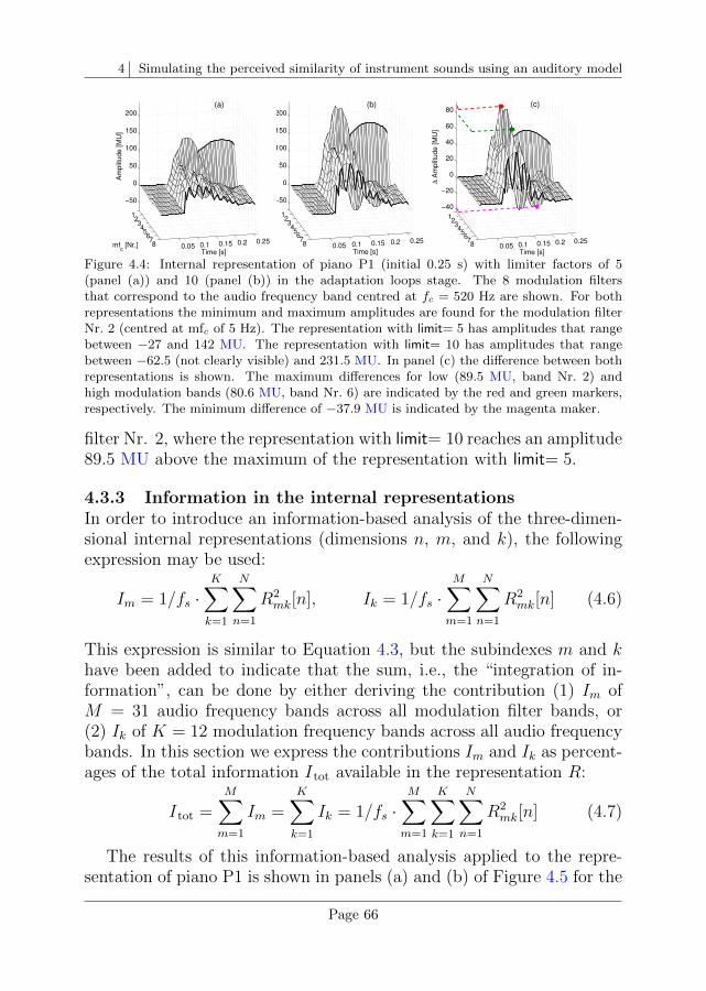
4 Simulating the perceived similarity of instrument sounds using an auditory model
0.05 0.1 0.15 0.2 0.2587
65
43
21
−50
0
50
100
150
200(a)
Time [s]mf
c [Nr.]
Am
plit
ud
e [
MU
]
0.05 0.1 0.15 0.2 0.2587
65
43
21
−50
0
50
100
150
200(b)
Time [s]
Am
plit
ud
e [
MU
]
0.05 0.1 0.15 0.2 0.2587
65
43
21
−40
−20
0
20
40
60
80(c)
Time [s]
∆ A
mp
litu
de
[M
U]
Figure 4.4: Internal representation of piano P1 (initial 0.25 s) with limiter factors of 5(panel (a)) and 10 (panel (b)) in the adaptation loops stage. The 8 modulation filtersthat correspond to the audio frequency band centred at fc = 520 Hz are shown. For bothrepresentations the minimum and maximum amplitudes are found for the modulation filterNr. 2 (centred at mfc of 5 Hz). The representation with limit= 5 has amplitudes that rangebetween −27 and 142 MU. The representation with limit= 10 has amplitudes that rangebetween −62.5 (not clearly visible) and 231.5 MU. In panel (c) the difference between bothrepresentations is shown. The maximum differences for low (89.5 MU, band Nr. 2) andhigh modulation bands (80.6 MU, band Nr. 6) are indicated by the red and green markers,respectively. The minimum difference of −37.9 MU is indicated by the magenta maker.
filter Nr. 2, where the representation with limit= 10 reaches an amplitude89.5 MU above the maximum of the representation with limit= 5.
4.3.3 Information in the internal representationsIn order to introduce an information-based analysis of the three-dimen-sional internal representations (dimensions n, m, and k), the followingexpression may be used:
Im = 1/fs ·K∑k=1
N∑n=1
R2mk[n], Ik = 1/fs ·
M∑m=1
N∑n=1
R2mk[n] (4.6)
This expression is similar to Equation 4.3, but the subindexes m and khave been added to indicate that the sum, i.e., the “integration of in-formation”, can be done by either deriving the contribution (1) Im ofM = 31 audio frequency bands across all modulation filter bands, or(2) Ik of K = 12 modulation frequency bands across all audio frequencybands. In this section we express the contributions Im and Ik as percent-ages of the total information Itot available in the representation R:
Itot =M∑m=1
Im =K∑k=1
Ik = 1/fs ·M∑m=1
K∑k=1
N∑n=1
R2mk[n] (4.7)
The results of this information-based analysis applied to the repre-sentation of piano P1 is shown in panels (a) and (b) of Figure 4.5 for the
Page 66
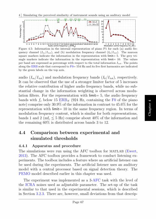
4 Simulating the perceived similarity of instrument sounds using an auditory model
Ch
ap
ter
4
3 4 5 6 7 8 9 1011121314151617181920212223242526272829303132330123456789
10
Audio centre frequency fc [ERB
N]
Perc
enta
ge [%
]
(a) lim=5
lim=10
554 1108 1662 2216 2770 3324 [Hz]
1 2 3 4 5 6 7 8 9 10 11 120
3
6
9
12
15
18
21
24
Pe
rce
nta
ge
[%
]
Modulation centre frequency mfc [Nr.]
(b)
Figure 4.5: Information in the internal representation of piano P1 for each (a) audio fre-quency channel (Im/Itot), and (b) modulation frequency channel (Ik/Itot). The maroonsquare markers indicate the information in the representation with limit= 5. The grey tri-angle markers indicate the information in the representation with limit= 10. The valuesper band are expressed as percentage with respect to the total information Itot. The pointsalong the ERB scale that correspond to F0= 554 Hz and its five first harmonics are indicatedby the green labels on the top axis.
audio (Im/Itot) and modulation frequency bands (Ik/Itot), respectively.It can be observed that the use of a stronger limiter factor of 5 increasesthe relative contribution of higher audio frequency bands, while no sub-stantial change in the information weighting is observed across modu-lation filters. For the representation with limit= 5, the audio frequencybands with fc below 15 ERBN (924 Hz, containing the F0 of the pianonote) comprise only 30.9% of the information in contrast to 45.6% for therepresentation with limit= 10 in the same frequency region. In terms ofmodulation frequency content, which is similar for both representations,bands 1 and 2 (mfc ≤ 5 Hz) comprise about 40% of the information andthe remaining 60% is distributed across bands 3 to 12.
4.4 Comparison between experimental andsimulated thresholds
4.4.1 Apparatus and procedure
The simulations were run using the AFC toolbox for MATLAB (Ewert,2013). The AFC toolbox provides a framework to conduct listening ex-periments. The toolbox includes a feature where an artificial listener canbe used during the experiments. The artificial listener uses an auditorymodel with a central processor based on signal detection theory. ThePEMO model described earlier in this chapter was used.
The experiment was implemented as a 3-AFC task with the level ofthe ICRA noises used as adjustable parameter. The set-up of the taskis similar to that used in the experimental sessions, which is describedin Section 3.2.3. There are, however, small deviations from that descrip-
Page 67
4 Simulating the perceived similarity of instrument sounds using an auditory model
tion, mainly aiming at reducing the simulation time. Two sounds arecompared: the target sound (presented once) and the reference sound(presented twice). The noise level was adjusted following a two-downone-up rule until 8 reversals are reached (4 reversals less than in theexperimental sessions). The step sizes were set to 4 dB, 2 dB (afterthe second reversal) and 1 dB (after the fourth reversal). The medianof the reversals during the measuring stage (last 4 reversals) is used toestimate the discrimination threshold of each pair of sounds. The pre-sentation level of the sounds was randomly varied (roved) by levels inthe range ±4 dB, drawn from a uniform distribution. The thresholdestimation was repeated 6 times for each condition.
4.4.2 Stimuli
Piano sounds
The same selection of Viennese piano recordings as in Chapter 3 wasused for the simulations. Recordings of the note C#5 (F0= 554 Hz)from seven pianos were used. One recording per piano was chosen lead-ing to a total of 7 stimuli. The sounds were set to have a duration of1.3 s and they were ramped-down using a 150-ms cosine ramp. They hada maximum loudness Smax of about 18 sone (refer to Table 3.1). Thepairwise comparison of all stimuli leads to a total of 21 possible combi-nations. For each piano pair 6 thresholds were simulated, 3 times thetarget piano was “A” and the reference piano was “B”, the remaining 3times the target piano was “B” and the reference piano was “A”.
Piano-weighted noises
The same ICRA noises (version A7) generated for the listening experi-ments of Chapter 3 were used in the simulations. For the comparison ofpianos “A” and “B” (or “B” and “A”) individual noises that follow thespectro-temporal properties of each piano were combined to generate apaired noise AB (refer to Section 3.2.2 for further details).
4.4.3 Exploratory simulations: Subset of piano sounds
At first, a subset of 9 (of the 21) available piano pairs was used forthe simulations. This selection was based on the results presented in
7In spite of the drawback in the spectral-matching properties (spectral tilt) of the ICRA-noisealgorithm version A, identified and briefly introduced in Chapter 3, the same ICRA noises areused in this chapter. We assume that any effect of the spectral tilt on the experimental results ofChapter 3 should also be tracked in the simulations of the current chapter. An in-depth analysis ofthe spectral tilt effect is presented in Chapter 5 by means of simulations using noises with (versionA) and without spectral tilt (“new” noises version B, adopted in Chapter 5).
Page 68
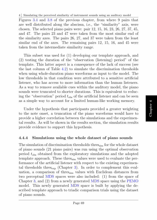
4 Simulating the perceived similarity of instrument sounds using an auditory model
Ch
ap
ter
4
Figures 3.4 and 3.8 of the previous chapter, from where 9 pairs thatare well distributed along the abscissa, i.e., the “similarity” axis, werechosen. The selected piano pairs were: pair 12, 15, 16, 23, 26, 27, 37, 45,and 47. The pairs 23 and 47 were taken from the most similar end ofthe similarity axes. The pairs 26, 27, and 37 were taken from the leastsimilar end of the axes. The remaining pairs 12, 15, 16, and 45 weretaken from the intermediate similarity range.
This subset was used for (1) developing our template approach, and(2) testing the duration of the “observation (listening) period” of thetemplate. This latter aspect is a consequence of the lack of success (seethe last column of Table 4.2) to simulate the discrimination thresholdswhen using whole-duration piano waveforms as input to the model. Thelow thresholds in that condition were attributed to a sensitive artificiallistener, who has access to more information than the human listeners.As a way to remove available cues within the auditory model, the pianosounds were truncated to shorter durations. This is equivalent to reduc-ing the “observation” period tobs of the artificial listener and can be seenas a simple way to account for a limited human-like working memory.
Under the hypothesis that participants provided a greater weightingto the note onset, a truncation of the piano waveforms would have toprovide a higher correlation between the simulations and the experimen-tal results. As will be shown in the results section, the simulation resultsprovide evidence to support this hypothesis.
4.4.4 Simulations using the whole dataset of piano sounds
The simulation of discrimination thresholds thressim for the whole datasetof piano sounds (21 piano pairs) was run using the optimal observationperiod tobs obtained from the exploratory simulations and the adoptedtemplate approach. These thressim values were used to evaluate the per-formance of the artificial listener with respect to the existing experimen-tal thresholds thresexp (Chapter 3). In order to complement this eval-uation, a comparison of thressim values with Euclidean distances fromtwo perceptual MDS spaces were also included: (1) from the space ofChapter 3, and (2) from a newly generated MDS space using the PEMOmodel. This newly generated MDS space is built by applying the de-scribed template approach to triadic comparison trials using the datasetof piano sounds.
Page 69
4 Simulating the perceived similarity of instrument sounds using an auditory model
Simulation of triadic comparisons using the current template approach
As described in Section 3.2.4, each triadic comparison trial consisted ofthree sounds that are labelled as “A”, “B”, and “C”. From this triad, outof the three pairs that can be formed (AB, AC, BC) the participant (theartificial listener) has to indicate which of the three pairs contains themost similar sounds and which one contains the least similar sounds. Inthis way, the remaining pair is labelled as having intermediate similarity.
To simulate this task, the whole dataset of pianos ((
73
)= 35 triads)
was used being restricted to the optimal tobs duration. No noise was usedbecause the experimental triadic comparisons were conducted in silence.Within each trial, three templates TA, TB, and TC were derived by nor-malising to unit energy the corresponding internal piano representationRA, RB, and RC . Two CCV values per pair were assessed (AB, AC,BC). For pair AB:
CCVAB =1
fs
Nobs∑n=1
RA[n] · TB[n], CCVBA =1
fs
Nobs∑n=1
RB[n] · TA[n]
where Nobs corresponds to the number of samples used by the artificiallistener to make the decision and is related to the optimal observationduration tobs. The CCV values for pair AC and BC can be obtained in a
similar manner. Finally, three CCV values were obtained, one for eachpair: CCVAB = max CCVAB,CCVBA+N1(µ, σ2)CCVAC = max CCVAC ,CCVCA+N2(µ, σ2)CCVBC = max CCVBC ,CCVCB+N3(µ, σ2) (4.8)
where Nx(µ, σ2), with x = 1, 2, 3 represents a similar internal noise as
used in Equation 4.5 that correspond to three numbers drawn from aGaussian distribution with µ = 0 and σ = 10.1 MU. The pair having the
maximum CCV value was indicated by the artificial listener as the most
similar pair. The pair having the minimum CCV value was indicated asthe least similar pair and, therefore, the remaining pair was indicatedas having intermediate similarity. Since no external (ICRA) noise isused in the trials, the CCV values are deterministic but the responses ofthe artificial listener were not due to the internal (Gaussian) noise. Tosimulate the triadic comparisons of 20 participants, the 35 triads wereevaluated 20 times by the artificial listener.
Page 70
4 Simulating the perceived similarity of instrument sounds using an auditory model
Ch
ap
ter
4
Table 4.2: Results of the simulations using a subset of 9 piano pairs and different tobs
durations. The minimum and maximum simulated thresholds are indicated together withtheir dynamic range (DR=thresmax−thresmin). The correlation values of the simulationswith the corresponding experimental data (taken from Figure 3.4) are given. The SNRrange of the experimental data is indicated in column Exp.
“Observation (listening) period” tobs [s]Parameter Exp. 0.2 0.25 0.3 0.5 0.7 0.9 1.1 1.3 1.5thresmax [dB] 20.75 15.0 20.5 14.25 9.25 5.0 3.25 2.5 2.0 2.75thresmin [dB] -1.75 -0.25 -1.0 1.5 -0.5 -1.25 -1.75 -2.75 -3.0 -2.5DR [dB] 22.5 15.25 21.5 12.75 9.75 6.25 5.0 5.25 5.0 5.25rp(7) − 0.66* 0.71* 0.65** 0.34 0.45 0.25 0.43 -0.21 -0.18rs(7) − 0.60** 0.78* 0.47 0.11 0.49 0.21 0.49 0.09 0.03
(*) Significant correlation, p < 0.05. (**) Correlations that approach significance, p < 0.10.
4.5 Results
Each piano pair was tested in a separate instrument-in-noise experiment.The simulation results are compared with the corresponding experimen-tal thresholds taken from Figure 3.4.
Experimental thresholds
The experimental thresholds of Figure 3.4 range between thresexp,max=20.75 dB (pair 23) and thresexp,min= −1.75 dB (pair 26), having a dy-namic range DRexp=thresexp,max−thresexp,min= 22.5 dB. Since the pairs23 and 26 are part of the subset of 9 piano pairs, this DR is also validfor the experimental thresholds using the subset of data.
4.5.1 Exploratory simulationsThe results for the selection of 9 piano pairs are shown in Table 4.2. Inthe table, information about the minimum (lowest median) and maxi-mum (highest median) estimated thresholds is shown. Their differenceis indicated as the dynamic range (DR) in dB. The simulations thatconsidered 1.5-s long piano sounds (whole duration of the sounds plus0.2 s of silence) delivered thresholds between thressim,max= 2.75 dB andthressim,min= −2.5 dB with a DR of 5.25 dB. These thresholds are toolow with respect to the experimental data. This means that the artificiallistener has access to more information than the actual participants. Asa way to remove available cues within the auditory model, the pianosounds were truncated to shorter durations. “Observation” durationstobs of 0.20, 0.25, 0.3, 0.5, 0.7, 0.9, 1.1, 1.3, and 1.50 s were tested. Theeffective duration of the piano sounds is 0.10 s shorter, because of theinitial silence in the waveforms. The tobs durations between 0.9 and 1.5 sseem to have a constant DR of about 5 dB and for shorter durations,
Page 71
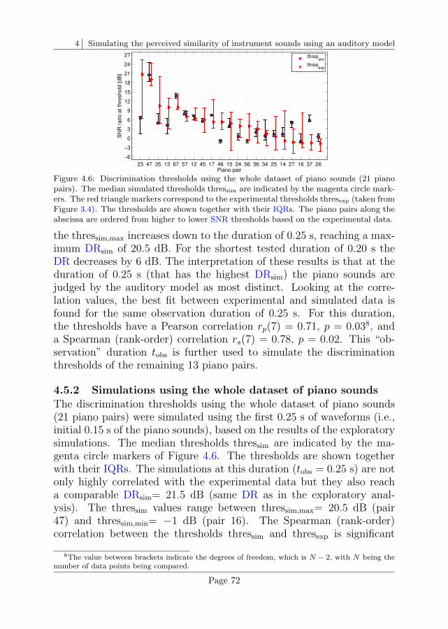
4 Simulating the perceived similarity of instrument sounds using an auditory model
23 47 35 13 67 57 12 45 17 46 15 24 56 36 34 25 14 27 16 37 26
−6
−3
0
3
6
9
12
15
18
21
24
27
Full dataset, 0.25−s
Piano pair
SN
R r
atio
at
thre
sh
old
[d
B]
thressim
thresexp
Figure 4.6: Discrimination thresholds using the whole dataset of piano sounds (21 pianopairs). The median simulated thresholds thressim are indicated by the magenta circle mark-ers. The red triangle markers correspond to the experimental thresholds thresexp (taken fromFigure 3.4). The thresholds are shown together with their IQRs. The piano pairs along theabscissa are ordered from higher to lower SNR thresholds based on the experimental data.
the thressim,max increases down to the duration of 0.25 s, reaching a max-imum DRsim of 20.5 dB. For the shortest tested duration of 0.20 s theDR decreases by 6 dB. The interpretation of these results is that at theduration of 0.25 s (that has the highest DRsim) the piano sounds arejudged by the auditory model as most distinct. Looking at the corre-lation values, the best fit between experimental and simulated data isfound for the same observation duration of 0.25 s. For this duration,the thresholds have a Pearson correlation rp(7) = 0.71, p = 0.038, anda Spearman (rank-order) correlation rs(7) = 0.78, p = 0.02. This “ob-servation” duration tobs is further used to simulate the discriminationthresholds of the remaining 13 piano pairs.
4.5.2 Simulations using the whole dataset of piano soundsThe discrimination thresholds using the whole dataset of piano sounds(21 piano pairs) were simulated using the first 0.25 s of waveforms (i.e.,initial 0.15 s of the piano sounds), based on the results of the exploratorysimulations. The median thresholds thressim are indicated by the ma-genta circle markers of Figure 4.6. The thresholds are shown togetherwith their IQRs. The simulations at this duration (tobs = 0.25 s) are notonly highly correlated with the experimental data but they also reacha comparable DRsim= 21.5 dB (same DR as in the exploratory anal-ysis). The thressim values range between thressim,max= 20.5 dB (pair47) and thressim,min= −1 dB (pair 16). The Spearman (rank-order)correlation between the thresholds thressim and thresexp is significant
8The value between brackets indicate the degrees of freedom, which is N − 2, with N being thenumber of data points being compared.
Page 72
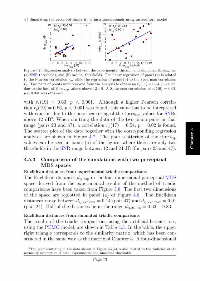
4 Simulating the perceived similarity of instrument sounds using an auditory model
Ch
ap
ter
4
−3 0 3 6 9 12 15 18 21
−3
0
3
6
9
12
15
18
21
thresexp
[dB]
thre
ssim
[dB
]
Regression analysis / Full dataset, 0.25−s
(a) rp(17)=0.54
(pval
=0.02)
1 3 5 7 9 11 13 15 17 19 211
3
5
7
9
11
13
15
17
19
21
thresexp
(ordinal)
thre
ssim
(ord
inal)
Regression analysis / Full dataset, 0.25−s
(b) rs(19)=0.63
(pval
<0.001)
Figure 4.7: Regression analysis between the experimental thresexp and simulated thressim as:(a) SNR thresholds, and (b) ordinal thresholds. The linear regression of panel (a) is relatedto the Pearson correlation rp, while the regression of panel (b) to the Spearman correlationrs. Two pairs of points were removed from the analysis to obtain an rp(17) = 0.54, p = 0.02,due to the lack of thresexp values above 12 dB. A Spearman correlation of rs(19) = 0.63,p < 0.001 was obtained.
with rs(19) = 0.63, p < 0.001. Although a higher Pearson correla-tion rp(19) = 0.66, p < 0.001 was found, this value has to be interpretedwith caution due to the poor scattering of the thresexp values for SNRsabove 12 dB9. When omitting the data of the two piano pairs in thatrange (pairs 23 and 47), a correlation rp(17) = 0.54, p = 0.02 is found.The scatter plot of the data together with the corresponding regressionanalyses are shown in Figure 4.7. The poor scattering of the thresexp
values can be seen in panel (a) of the figure, where there are only twothresholds in the SNR range between 12 and 24 dB (for pairs 23 and 47).
4.5.3 Comparison of the simulations with two perceptualMDS spaces
Euclidean distances from experimental triadic comparisons
The Euclidean distances dij exp in the four-dimensional perceptual MDSspace derived from the experimental results of the method of triadiccomparisons have been taken from Figure 3.8. The first two dimensionsof the space are replotted in panel (a) of Figure 4.8. The Euclideandistances range between dij exp,min = 0.14 (pair 47) and dij exp,max = 0.91(pair 24). Half of the distances lie in the range dij,25−75 = 0.63− 0.83.
Euclidean distances from simulated triadic comparisons
The results of the triadic comparisons using the artificial listener, i.e.,using the PEMO model, are shown in Table 4.3. In the table, the upperright triangle corresponds to the similarity matrix, which has been con-structed in the same way as the matrix of Chapter 3. A four-dimensional
9The poor scattering of the data shown in Figure 4.7(a) is also related to the violation of thenormality assumption of both, experimental and simulated thresholds.
Page 73
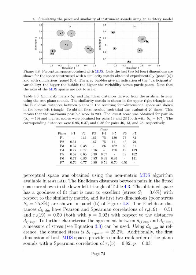
4 Simulating the perceived similarity of instrument sounds using an auditory model
−0.4 −0.2 0 0.2 0.4 0.6
−0.4
−0.2
0
0.2
0.4
0.6
1
23
4
5
6
7
Dimension 1
Dim
en
sio
n 2
(a)
−0.4 −0.2 0 0.2 0.4 0.6
−0.4
−0.2
0
0.2
0.4
0.6
12 3
4
5
6
7
Dimension 1
Dim
en
sio
n 2
(b)
Figure 4.8: Perceptual spaces obtained with MDS. Only the first two (of four) dimensions areshown for the space constructed with a similarity matrix obtained experimentally (panel (a))and with simulations (panel (b)). The grey bubbles give an indication of the “participant’s”variability: the bigger the bubble the higher the variability across participants. Note thatthe axes of the MDS spaces are not to scale.
Table 4.3: Similarity matrix Sij and Euclidean distances derived from the artificial listenerusing the test piano sounds. The similarity matrix is shown in the upper right triangle andthe Euclidean distances between pianos in the resulting four-dimensional space are shownin the lower left triangle. To obtain these results, each triad was evaluated 20 times. Thismeans that the maximum possible score is 200. The lowest score was obtained for pair 46(Sij = 19) and highest scores were obtained for pairs 13 and 23 (both with Sij = 167). Thecorresponding distances were 0.95, 0.37, and 0.38 for pairs 46, 13, and 23, respectively.
Piano
Piano P1 P2 P3 P4 P5 P6 P7P1 - 145 167 75 130 77 83P2 0.51 - 167 75 111 45 79P3 0.37 0.38 - 86 162 59 61P4 0.77 0.77 0.76 - 128 19 139P5 0.57 0.65 0.38 0.57 - 49 102P6 0.77 0.86 0.83 0.95 0.84 - 141P7 0.76 0.77 0.80 0.51 0.70 0.51 -
perceptual space was obtained using the non-metric MDS algorithmavailable in MATLAB. The Euclidean distances between pairs in the fittedspace are shown in the lower left triangle of Table 4.3. The obtained spacehas a goodness of fit that is near to excellent (stress St = 3.6%) withrespect to the similarity matrix, and its first two dimensions (poor stressSt = 25.8%) are shown in panel (b) of Figure 4.8. The Euclidean dis-tances dij sim have Pearson and Spearman correlations of rp(19) = 0.51and rs(19) = 0.50 (both with p = 0.02) with respect to the distancesdij exp. To further characterise the agreement between dij exp and dij sim,a measure of stress (see Equation 3.3) can be used. Using dij exp as ref-erence, the obtained stress is St exp-sim = 25.2%. Additionally, the firstdimension of both MDS spaces provide a similar rank order of the pianosounds with a Spearman correlation of rs(5) = 0.82, p = 0.03.
Page 74
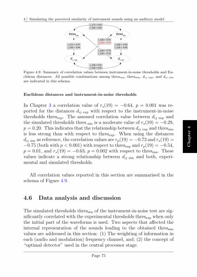
4 Simulating the perceived similarity of instrument sounds using an auditory model
Ch
ap
ter
4
Figure 4.9: Summary of correlation values between instrument-in-noise thresholds and Eu-clidean distances. All possible combinations among thresexp, thressim, dij exp, and dij sim
are indicated in this schema.
Euclidean distances and instrument-in-noise thresholds
In Chapter 3 a correlation value of rs(19) = −0.64, p = 0.001 was re-ported for the distances dij exp with respect to the instrument-in-noisethresholds thresexp. The assessed correlation value between dij exp andthe simulated thresholds thres sim is a moderate value of rs(19) = −0.29,p = 0.20. This indicates that the relationship between dij exp and thressim
is less strong than with respect to thresexp. When using the distancesdij sim as reference, the correlation values are rp(19) = −0.73 and rs(19) =−0.75 (both with p < 0.001) with respect to thresexp and rp(19) = −0.54,p = 0.01, and rs(19) = −0.63, p = 0.002 with respect to thressim. Thesevalues indicate a strong relationship between dij sim and both, experi-mental and simulated thresholds.
All correlation values reported in this section are summarised in theschema of Figure 4.9.
4.6 Data analysis and discussion
The simulated thresholds thressim of the instrument-in-noise test are sig-nificantly correlated with the experimental thresholds thresexp when onlythe initial part of the waveforms is used. Two aspects that affected theinternal representation of the sounds leading to the obtained thressim
values are addressed in this section: (1) The weighting of information ineach (audio and modulation) frequency channel, and; (2) the concept of“optimal detector” used in the central processor stage.
Page 75
4 Simulating the perceived similarity of instrument sounds using an auditory model
4.6.1 Weighting of information in the internalrepresentations
The weighting of information for each audio and modulation frequencyband within the PEMO model is inherently introduced when using theconcept of memory template. This weighting depends on the “expectedsignal” to be discriminated and the processing introduced by each stageof the auditory model. Two aspects that may have affected the weightingof information in our approach are discussed: (1) the stronger limitationintroduced in the adaptation loops, and (2) the processing of sounds thathave shorter durations.
Our decision stage made use of two criteria, i.e., two expected sig-nals that lead to two templates Tp,t and Tp,r. Since the decision is basedon CCV values, where the contribution of information to the differencerepresentation ∆Rx is weighted using Tp,t and Tp,r, the contribution ofindividual (audio and modulation) frequency bands to each CCVx valuecan be assessed. Following a similar approach to that used to analysethe piano-alone representation R of piano P1 (shown in Figure 4.5), theweighting of information that is introduced within the auditory modelcan be obtained by assessing the percentual contribution of the template-weighted piano representations ∆Rx ·Tp (from Equation 4.3) using Equa-tions 4.6 and 4.7. The contribution of each frequency band (Im/Itot foraudio frequencies and Ik/Itot for modulation frequencies) in the follow-ing conditions is considered: (1) when the adaptation loops are limitedusing a factor of 5 (as suggested in this thesis) and with a factor of 10(as in the literature), and (2) considering the total duration of the piano-plus-noise sounds (1.5 s) and when only the first 0.25 s are evaluated.In this analysis, all 21 piano pairs were included. Since our interest ison the weighting of information at threshold, the difference representa-tion ∆R = R−RN is assessed at the noise level of the respective ICRAnoise indicated by the simulated thresholds. The information-weightedvalues (Im/Itot and Ik/Itot) for the comparison between limiter factorsare shown in Figure 4.10. The values Im and Ik were obtained as themedian of 42 values (21 pairs with one value using Tp,t and one valueusing Tp,r). The error bars indicate their IQRs. The weighting Im/Itot
shown in panel (a) shows that by using a stronger limiter factor, theinformation of higher audio frequency bands receive a higher relativeweighting. For a limiter factor of 10, the weighting seems to be verysimilar to the distribution of information for the piano-alone representa-tion shown in panel (a) of Figure 4.5. The information contribution of
Page 76
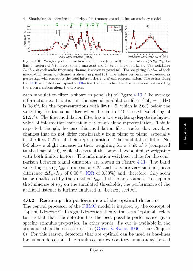
4 Simulating the perceived similarity of instrument sounds using an auditory model
Ch
ap
ter
4
3 4 5 6 7 8 9 101112131415161718192021222324252627282930313233
0
2
4
6
8
10
12
14
16
Audio centre frequency fc [ERB
N]
Perc
enta
ge [%
]
(a) lim=5
lim=10
554 1108 1662 2216 2770 3324 [Hz]
1 2 3 4 5 6 7 8 9 10 11 120
3
6
9
12
15
18
21
24
27
Pe
rce
nta
ge
[%
]
Modulation centre frequency mfc [Nr.]
(b)
Figure 4.10: Weighting of information in difference (internal) representations (∆Rx ·Tp) forlimiter factors of 5 (maroon square markers) and 10 (grey circle markers). The weightingIm/Itot of each audio frequency channel is shown in panel (a). The weighting Ik/Itot of eachmodulation frequency channel is shown in panel (b). The values per band are expressed aspercentage with respect to the total information Itot of each representation. The points alongthe ERB scale that correspond to F0= 554 Hz and its five first harmonics are indicated bythe green numbers along the top axis.
each modulation filter is shown in panel (b) of Figure 4.10. The averageinformation contribution in the second modulation filter (mfc = 5 Hz)is 18.6% for the representations with limit= 5, which is 2.6% below theweighting for the same filter when the limit of 10 is used (weighting of21.2%). The first modulation filter has a low weighting despite its highervalue of information content in the piano-alone representation. This isexpected, though, because this modulation filter tracks slow envelopechanges that do not differ considerably from piano to piano, especiallyin the first 0.25 s of their representation. The modulation filters Nr.6-9 show a slight increase in their weighting for a limit of 5 (comparedto the limit of 10), while the rest of the bands have a similar weightingwith both limiter factors. The information-weighted values for the com-parison between signal durations are shown in Figure 4.11. The bandweightings using tobs durations of 0.25 and 1.5 s are very similar (meandifference ∆Im/Itot of 0.00%, IQR of 0.33%) and, therefore, they seemto be unaffected by the duration tobs of the piano sounds. To explainthe influence of tobs on the simulated thresholds, the performance of theartificial listener is further analysed in the next section.
4.6.2 Reducing the performance of the optimal detectorThe central processor of the PEMO model is inspired by the concept of“optimal detector”. In signal detection theory, the term “optimal” refersto the fact that the detector has the best possible performance givenspecific stimulus properties. In other words, if a cue is available in thestimulus, then the detector uses it (Green & Swets, 1966, their Chapter6). For this reason, detectors that are optimal can be used as baselinesfor human detection. The results of our exploratory simulations showed
Page 77
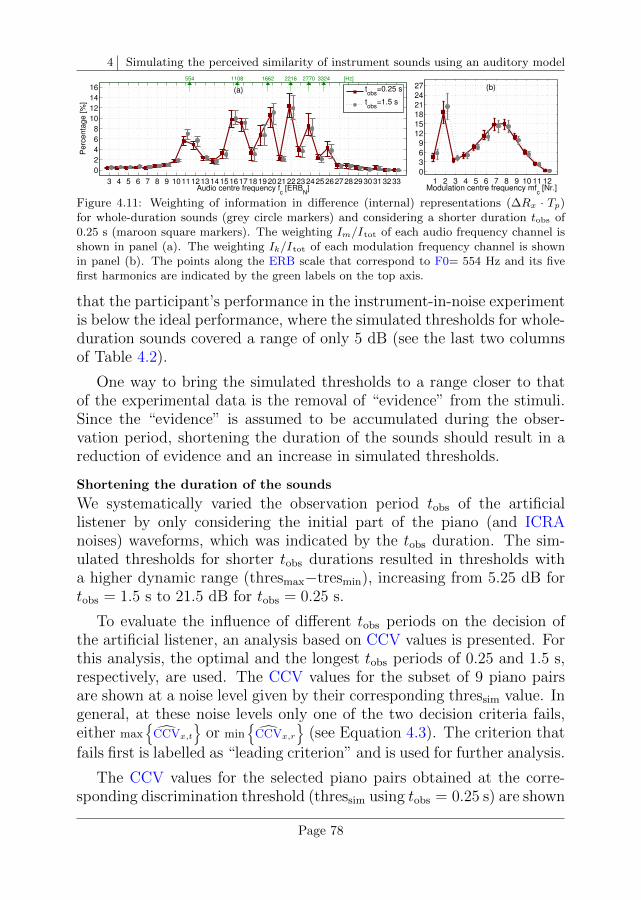
4 Simulating the perceived similarity of instrument sounds using an auditory model
3 4 5 6 7 8 9 101112131415161718192021222324252627282930313233
0
2
4
6
8
10
12
14
16
Audio centre frequency fc [ERB
N]
Perc
enta
ge [%
]
(a) tobs
=0.25 s
tobs
=1.5 s
554 1108 1662 2216 2770 3324 [Hz]
1 2 3 4 5 6 7 8 9 10 11 120
3
6
9
12
15
18
21
24
27
Pe
rce
nta
ge
[%
]
Modulation centre frequency mfc [Nr.]
(b)
Figure 4.11: Weighting of information in difference (internal) representations (∆Rx · Tp)for whole-duration sounds (grey circle markers) and considering a shorter duration tobs of0.25 s (maroon square markers). The weighting Im/Itot of each audio frequency channel isshown in panel (a). The weighting Ik/Itot of each modulation frequency channel is shownin panel (b). The points along the ERB scale that correspond to F0= 554 Hz and its fivefirst harmonics are indicated by the green labels on the top axis.
that the participant’s performance in the instrument-in-noise experimentis below the ideal performance, where the simulated thresholds for whole-duration sounds covered a range of only 5 dB (see the last two columnsof Table 4.2).
One way to bring the simulated thresholds to a range closer to thatof the experimental data is the removal of “evidence” from the stimuli.Since the “evidence” is assumed to be accumulated during the obser-vation period, shortening the duration of the sounds should result in areduction of evidence and an increase in simulated thresholds.
Shortening the duration of the sounds
We systematically varied the observation period tobs of the artificiallistener by only considering the initial part of the piano (and ICRAnoises) waveforms, which was indicated by the tobs duration. The sim-ulated thresholds for shorter tobs durations resulted in thresholds witha higher dynamic range (thresmax−tresmin), increasing from 5.25 dB fortobs = 1.5 s to 21.5 dB for tobs = 0.25 s.
To evaluate the influence of different tobs periods on the decision ofthe artificial listener, an analysis based on CCV values is presented. Forthis analysis, the optimal and the longest tobs periods of 0.25 and 1.5 s,respectively, are used. The CCV values for the subset of 9 piano pairsare shown at a noise level given by their corresponding thressim value. Ingeneral, at these noise levels only one of the two decision criteria fails,either max
CCVx,t
or min
CCVx,r
(see Equation 4.3). The criterion that
fails first is labelled as “leading criterion” and is used for further analysis.
The CCV values for the selected piano pairs obtained at the corre-sponding discrimination threshold (thressim using tobs = 0.25 s) are shown
Page 78
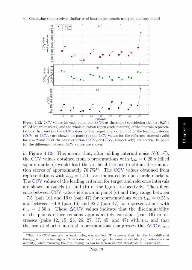
4 Simulating the perceived similarity of instrument sounds using an auditory model
Ch
ap
ter
4
12 15 16 23 26 27 37 45 47
102030405060708090
100110120130140150160
Piano pair
CC
V1 o
f th
e
leadin
g c
rite
rion
(a)
0 −0.25 s
0 −1.50 s
12 15 16 23 26 27 37 45 47
10203040506070
Piano pair
CC
V2,3
of th
e
leadin
g c
rite
rion (b)
12 15 16 23 26 27 37 45 47
−100
1020304050607080
Piano pair
∆ C
CV
(c)
Figure 4.12: CCV values for each piano pair (SNR at threshold) considering the first 0.25 s(filled square markers) and the whole duration (open circle markers) of the internal represen-tations. In panel (a) the CCV values for the target interval (x = 1) of the leading criterion(CCVt or CCVr) are shown. In panel (b) the CCV values for the reference interval (validfor x = 2 and 3) of the same criterion (CCVt or CCVr, respectively) are shown. In panel(c) the difference between CCV values are shown.
in Figure 4.12. This means that, after adding internal noise N(0, σ2),the CCV values obtained from representations with tobs = 0.25 s (filledsquare markers) would lead the artificial listener to obtain discrimina-tion scores of approximately 70.7%10. The CCV values obtained fromrepresentations with tobs = 1.50 s are indicated by open circle markers.The CCV values of the leading criterion for target and reference intervalsare shown in panels (a) and (b) of the figure, respectively. The differ-ence between CCV values is shown in panel (c) and they range between−7.5 (pair 16) and 16.0 (pair 47) for representations with tobs = 0.25 sand between −4.8 (pair 16) and 82.7 (pair 47) for representations withtobs = 1.50 s. These ∆CCV values indicate that the discriminabilityof the pianos either remains approximately constant (pair 16) or in-creases (pairs 12, 15, 23, 26, 27, 37, 45, and 47) with tobs and thatthe use of shorter internal representations compresses the ∆CCV0.25 s
10For this CCV analysis no level roving was applied. This means that the discriminability atthressim is in practice higher. This is due to, on average, the lower thresholds (i.e., better discrim-inability) when removing the level roving, as can be seen in no-rove thresholds of Figure 4.13.
Page 79
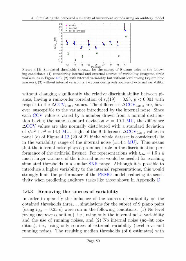
4 Simulating the perceived similarity of instrument sounds using an auditory model
12 15 16 23 26 27 37 45 47
−15
−12
−9
−6
−3
0
3
6
9
12
15
18
21
24
Piano pair
thre
ssim
[d
B]
ext+int
no−rove
no−int (only ext)
Figure 4.13: Simulated thresholds thressim for the subset of 9 piano pairs in the follow-ing conditions: (1) considering internal and external sources of variability (magenta circlemarkers, as in Figure 4.6); (2) with internal variability but without level roving (square bluemarkers); (3) without internal variability, i.e., considering only sources of external variability.
without changing significantly the relative discriminability between pi-anos, having a rank-order correlation of rs(19) = 0.93, p < 0.001 withrespect to the ∆CCV1.50 s values. The differences ∆CCV0.25 s are, how-ever, susceptible to the variance introduced by the internal noise. Sinceeach CCV value is varied by a number drawn from a normal distribu-tion having the same standard deviation σ = 10.1 MU, the difference∆CCV values are also normally distributed with a standard deviationof√σ2 + σ2 = 14.4 MU. Eight of the 9 difference ∆CCV0.25 s values in
panel (c) of Figure 4.12 (20 of 21 if the whole dataset is considered) liein the variability range of the internal noise (±14.4 MU). This meansthat the internal noise plays a prominent role in the discrimination per-formance of the artificial listener. For representations with tobs = 1.5 s amuch larger variance of the internal noise would be needed for reachingsimulated thresholds in a similar SNR range. Although it is possible tointroduce a higher variability to the internal representations, this wouldstrongly limit the performance of the PEMO model, reducing its sensi-tivity when predicting auditory tasks like those shown in Appendix D.
4.6.3 Removing the sources of variability
In order to quantify the influence of the sources of variability on theobtained thresholds thressim, simulations for the subset of 9 piano pairs(using tobs = 0.25 s) were run in the following conditions: (1) No levelroving (no–rove condition), i.e., using only the internal noise variabilityand the use of running noises, and (2) No internal noise (no–int con-dition), i.e., using only sources of external variability (level rove andrunning noise). The resulting median thresholds (of 6 estimates) with
Page 80
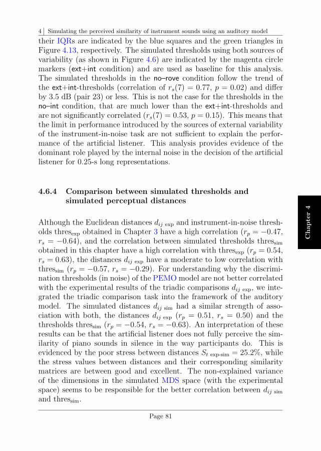
4 Simulating the perceived similarity of instrument sounds using an auditory model
Ch
ap
ter
4
their IQRs are indicated by the blue squares and the green triangles inFigure 4.13, respectively. The simulated thresholds using both sources ofvariability (as shown in Figure 4.6) are indicated by the magenta circlemarkers (ext+int condition) and are used as baseline for this analysis.The simulated thresholds in the no–rove condition follow the trend ofthe ext+int-thresholds (correlation of rs(7) = 0.77, p = 0.02) and differby 3.5 dB (pair 23) or less. This is not the case for the thresholds in theno–int condition, that are much lower than the ext+int-thresholds andare not significantly correlated (rs(7) = 0.53, p = 0.15). This means thatthe limit in performance introduced by the sources of external variabilityof the instrument-in-noise task are not sufficient to explain the perfor-mance of the artificial listener. This analysis provides evidence of thedominant role played by the internal noise in the decision of the artificiallistener for 0.25-s long representations.
4.6.4 Comparison between simulated thresholds andsimulated perceptual distances
Although the Euclidean distances dij exp and instrument-in-noise thresh-olds thresexp obtained in Chapter 3 have a high correlation (rp = −0.47,rs = −0.64), and the correlation between simulated thresholds thressim
obtained in this chapter have a high correlation with thresexp (rp = 0.54,rs = 0.63), the distances dij exp have a moderate to low correlation withthressim (rp = −0.57, rs = −0.29). For understanding why the discrimi-nation thresholds (in noise) of the PEMO model are not better correlatedwith the experimental results of the triadic comparisons dij exp, we inte-grated the triadic comparison task into the framework of the auditorymodel. The simulated distances dij sim had a similar strength of asso-ciation with both, the distances dij exp (rp = 0.51, rs = 0.50) and thethresholds thressim (rp = −0.54, rs = −0.63). An interpretation of theseresults can be that the artificial listener does not fully perceive the sim-ilarity of piano sounds in silence in the way participants do. This isevidenced by the poor stress between distances St exp-sim = 25.2%, whilethe stress values between distances and their corresponding similaritymatrices are between good and excellent. The non-explained varianceof the dimensions in the simulated MDS space (with the experimentalspace) seems to be responsible for the better correlation between dij sim
and thressim.
Page 81
4 Simulating the perceived similarity of instrument sounds using an auditory model
4.7 Conclusions
In this chapter an auditory model was used to simulate the discrimina-tion thresholds between recorded sounds of one note (C#5) played on 7different pianos. In order to compare two internal (piano) representa-tions, two memory templates were required to allow the artificial listener(PEMO model) to distinguish one piano from another. The need of themodel to access the representation of the sounds being compared can beinterpreted as an approach that resembles a recognition rather than adiscrimination task. The obtained thressim values from the model weresignificantly correlated with the thresexp values when only the initial partof the waveforms was used. An optimal “observation” duration tobs of0.25 s was found. We hypothesise however that other tobs durations willbe obtained if other (piano) notes are tested. The relevant aspect is thata reduction in the amount of information available to the artificial lis-tener brought the simulated and experimental data to a closer range. Inthis context, the success of the simulations might be interpreted in thefollowing way: (1) Using longer tobs durations, the artificial listener hasaccess to more cues than the actual participants. This may be related tothe fact that the central processor integrates the incoming information“optimally”; (2) the shorter the tobs duration the less information can beintegrated by the artificial listener. The performance of the artificial lis-tener is limited by the internal noise of the auditory model and by othersources of (external) variability that are related to the instrument-in-noise task. These sources of external variability are the randomisationof the presentation level of each interval (level roving) and the use ofrunning ICRA noises. The most dominant of the sources of variability isthe internal noise in the auditory model, especially for intervals with atobs of 0.25 s and SNR levels around or above the simulated thresholds.The results presented in this chapter support the idea that the unifiedframework offered by the PEMO model can be used to evaluate percep-tual tasks using complex sounds. This can be seen as an extension ofthe use of this type of models and their success relies on the adjustmentof the central processor stage included within the model, in combinationwith an appropriate representation of sources of internal noise.
Page 82
5 Measuring and simulating the similarity of in-strument sounds in a reverberant environment1
5.1 Introduction
The perceptual similarity task studied in the previous chapters is appliedhere to the same set of piano sounds but after being convolved with theimpulse response of a reverberant room. Although the judgements forthe new reverberant sounds are expected to be somewhat correlated withthe results reported in Chapter 3, relative similarity changes among pi-anos due to reverberation are expected to be tracked by the instrument-in-noise method and by simulations using the auditory (PEMO) modeldescribed in Chapter 4. One of the objectives of the study case presentedin this chapter is, therefore, to extend the use of the experimental andcomputational frameworks presented in Chapters 3 and 4. The experi-mental data of the instrument-in-noise method using reverberant soundsare compared with the method of triadic comparisons and with simu-lations of the discrimination thresholds using the PEMO model. As adifference to the procedures of the previous chapters, a new version (ver-sion B) of the ICRA noise algorithm has been adopted. Version B ofthe algorithm corrects the spectral tilt towards high frequencies that thealgorithm version A had (see Section 3.5). For this reason, a secondobjective of this chapter is to quantify the effect of using ICRA noiseswith different spectral properties. The evaluation is done by comparingsimulated discrimination thresholds using the two ICRA noise versions.
5.2 Description of the method
The experimental methods and the computational framework used inthe study case presented in this chapter are very similar to those usedin Chapters 3 and 4, respectively. The set of stimuli comprises the same
1This chapter is partly based on: A. Osses, and A. Kohlrausch (2018, submitted). Auditorymodelling of the perceptual similarity between piano sounds. Acta Acust. united Ac.
Page 83
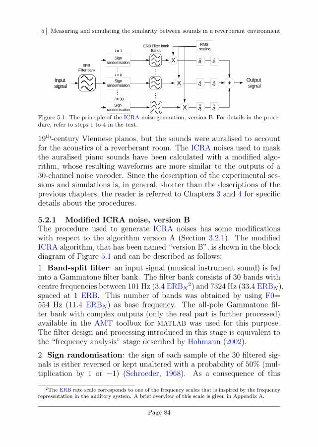
5 Measuring and simulating the similarity between sounds in a reverberant environment
Figure 5.1: The principle of the ICRA noise generation, version B. For details in the proce-dure, refer to steps 1 to 4 in the text.
19th-century Viennese pianos, but the sounds were auralised to accountfor the acoustics of a reverberant room. The ICRA noises used to maskthe auralised piano sounds have been calculated with a modified algo-rithm, whose resulting waveforms are more similar to the outputs of a30-channel noise vocoder. Since the description of the experimental ses-sions and simulations is, in general, shorter than the descriptions of theprevious chapters, the reader is referred to Chapters 3 and 4 for specificdetails about the procedures.
5.2.1 Modified ICRA noise, version BThe procedure used to generate ICRA noises has some modificationswith respect to the algorithm version A (Section 3.2.1). The modifiedICRA algorithm, that has been named “version B”, is shown in the blockdiagram of Figure 5.1 and can be described as follows:
1. Band-split filter: an input signal (musical instrument sound) is fedinto a Gammatone filter bank. The filter bank consists of 30 bands withcentre frequencies between 101 Hz (3.4 ERBN
2) and 7324 Hz (33.4 ERBN),spaced at 1 ERB. This number of bands was obtained by using F0=554 Hz (11.4 ERBN) as base frequency. The all-pole Gammatone fil-ter bank with complex outputs (only the real part is further processed)available in the AMT toolbox for MATLAB was used for this purpose.The filter design and processing introduced in this stage is equivalent tothe “frequency analysis” stage described by Hohmann (2002).
2. Sign randomisation: the sign of each sample of the 30 filtered sig-nals is either reversed or kept unaltered with a probability of 50% (mul-tiplication by 1 or −1) (Schroeder, 1968). As a consequence of this
2The ERB rate scale corresponds to one of the frequency scales that is inspired by the frequencyrepresentation in the auditory system. A brief overview of this scale is given in Appendix A.
Page 84
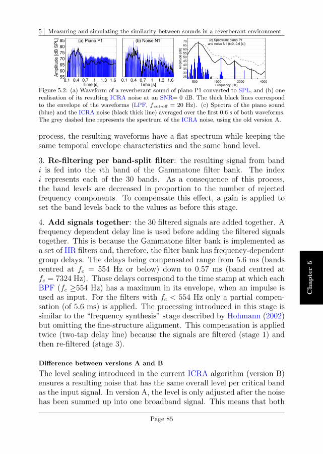
5 Measuring and simulating the similarity between sounds in a reverberant environment
Ch
ap
ter
5
0.1 0.4 0.7 1 1.3 1.655
60
65
70
75
80
85
Am
plit
ude [dB
SP
L]
Time [s]
(a) Piano P1
0.1 0.4 0.7 1 1.3 1.6Time [s]
(b) Noise N1
500 1000 2000 4000
25
30
35
40
45
50
55
60
65
70
Frequency [Hz]
Am
plit
ude [dB
]
(c) Spectrum: piano P1 and noise N1 (t=0−0.6 [s])
Figure 5.2: (a) Waveform of a reverberant sound of piano P1 converted to SPL, and (b) onerealisation of its resulting ICRA noise at an SNR= 0 dB. The thick black lines correspondto the envelope of the waveforms (LPF, fcut-off = 20 Hz). (c) Spectra of the piano sound(blue) and the ICRA noise (black thick line) averaged over the first 0.6 s of both waveforms.The grey dashed line represents the spectrum of the ICRA noise, using the old version A.
process, the resulting waveforms have a flat spectrum while keeping thesame temporal envelope characteristics and the same band level.
3. Re-filtering per band-split filter: the resulting signal from bandi is fed into the ith band of the Gammatone filter bank. The indexi represents each of the 30 bands. As a consequence of this process,the band levels are decreased in proportion to the number of rejectedfrequency components. To compensate this effect, a gain is applied toset the band levels back to the values as before this stage.
4. Add signals together: the 30 filtered signals are added together. Afrequency dependent delay line is used before adding the filtered signalstogether. This is because the Gammatone filter bank is implemented asa set of IIR filters and, therefore, the filter bank has frequency-dependentgroup delays. The delays being compensated range from 5.6 ms (bandscentred at fc = 554 Hz or below) down to 0.57 ms (band centred atfc = 7324 Hz). Those delays correspond to the time stamp at which eachBPF (fc ≥554 Hz) has a maximum in its envelope, when an impulse isused as input. For the filters with fc < 554 Hz only a partial compen-sation (of 5.6 ms) is applied. The processing introduced in this stage issimilar to the “frequency synthesis” stage described by Hohmann (2002)but omitting the fine-structure alignment. This compensation is appliedtwice (two-tap delay line) because the signals are filtered (stage 1) andthen re-filtered (stage 3).
Difference between versions A and B
The level scaling introduced in the current ICRA algorithm (version B)ensures a resulting noise that has the same overall level per critical bandas the input signal. In version A, the level is only adjusted after the noisehas been summed up into one broadband signal. This means that both
Page 85
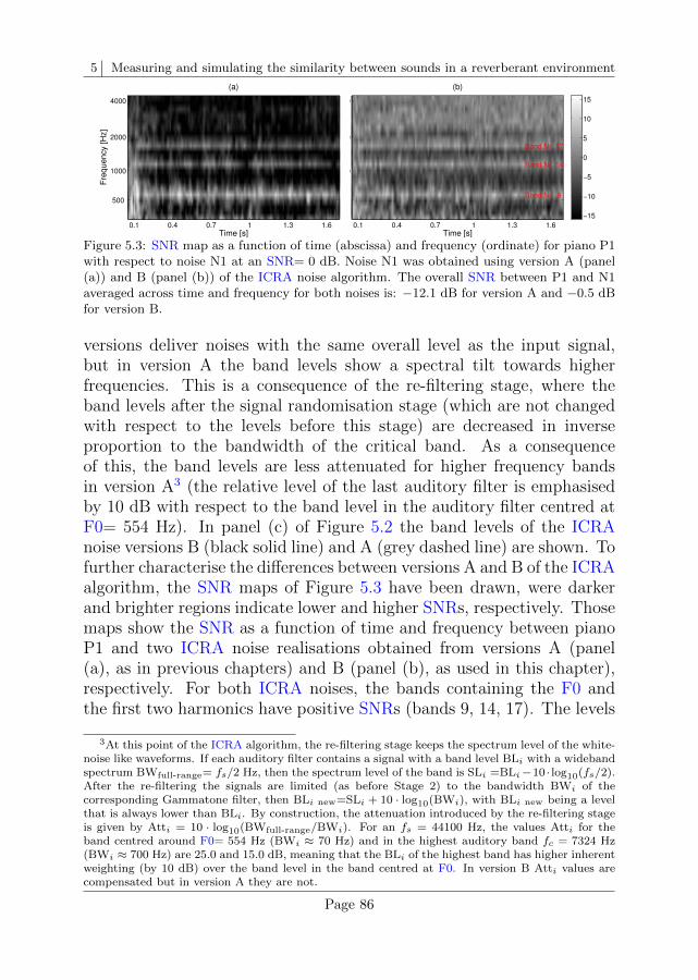
5 Measuring and simulating the similarity between sounds in a reverberant environment
Time [s]
Fre
quency [H
z]
(a)
0.1 0.4 0.7 1 1.3 1.6
500
1000
2000
4000
−15
−10
−5
0
5
10
15
Time [s]
Fre
quency [H
z]
(b)
Band Nr. 9
Band Nr. 14
Band Nr. 17
0.1 0.4 0.7 1 1.3 1.6
500
1000
2000
4000
−15
−10
−5
0
5
10
15
Figure 5.3: SNR map as a function of time (abscissa) and frequency (ordinate) for piano P1with respect to noise N1 at an SNR= 0 dB. Noise N1 was obtained using version A (panel(a)) and B (panel (b)) of the ICRA noise algorithm. The overall SNR between P1 and N1averaged across time and frequency for both noises is: −12.1 dB for version A and −0.5 dBfor version B.
versions deliver noises with the same overall level as the input signal,but in version A the band levels show a spectral tilt towards higherfrequencies. This is a consequence of the re-filtering stage, where theband levels after the signal randomisation stage (which are not changedwith respect to the levels before this stage) are decreased in inverseproportion to the bandwidth of the critical band. As a consequenceof this, the band levels are less attenuated for higher frequency bandsin version A3 (the relative level of the last auditory filter is emphasisedby 10 dB with respect to the band level in the auditory filter centred atF0= 554 Hz). In panel (c) of Figure 5.2 the band levels of the ICRAnoise versions B (black solid line) and A (grey dashed line) are shown. Tofurther characterise the differences between versions A and B of the ICRAalgorithm, the SNR maps of Figure 5.3 have been drawn, were darkerand brighter regions indicate lower and higher SNRs, respectively. Thosemaps show the SNR as a function of time and frequency between pianoP1 and two ICRA noise realisations obtained from versions A (panel(a), as in previous chapters) and B (panel (b), as used in this chapter),respectively. For both ICRA noises, the bands containing the F0 andthe first two harmonics have positive SNRs (bands 9, 14, 17). The levels
3At this point of the ICRA algorithm, the re-filtering stage keeps the spectrum level of the white-noise like waveforms. If each auditory filter contains a signal with a band level BLi with a widebandspectrum BWfull-range= fs/2 Hz, then the spectrum level of the band is SLi =BLi−10 · log10(fs/2).After the re-filtering the signals are limited (as before Stage 2) to the bandwidth BWi of thecorresponding Gammatone filter, then BLi new=SLi + 10 · log10(BWi), with BLi new being a levelthat is always lower than BLi. By construction, the attenuation introduced by the re-filtering stageis given by Atti = 10 · log10(BWfull-range/BWi). For an fs = 44100 Hz, the values Atti for theband centred around F0= 554 Hz (BWi ≈ 70 Hz) and in the highest auditory band fc = 7324 Hz(BWi ≈ 700 Hz) are 25.0 and 15.0 dB, meaning that the BLi of the highest band has higher inherentweighting (by 10 dB) over the band level in the band centred at F0. In version B Atti values arecompensated but in version A they are not.
Page 86
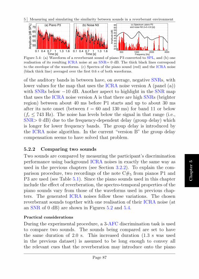
5 Measuring and simulating the similarity between sounds in a reverberant environment
Ch
ap
ter
5
0.1 0.4 0.7 1 1.3 1.6
50
55
60
65
70A
mp
litu
de
[d
B S
PL
]
Time [s]
(a) Piano P3
0.1 0.4 0.7 1 1.3 1.6Time [s]
(b) Noise N3
500 1000 2000 4000
20
25
30
35
40
45
50
55
60
65
Frequency [Hz]
Am
plit
ud
e [
dB
]
(c) Spectrum: piano P3 and noise N3 (t=0−0.6 [s])
Figure 5.4: (a) Waveform of a reverberant sound of piano P3 converted to SPL, and (b) onerealisation of its resulting ICRA noise at an SNR= 0 dB. The thick black lines correspondto the envelope of the waveforms. (c) Spectra of the piano sound (red) and the ICRA noise(black thick line) averaged over the first 0.6 s of both waveforms.
of the auditory bands in between have, on average, negative SNRs, withlower values for the map that uses the ICRA noise version A (panel (a))with SNRs below −10 dB. Another aspect to highlight in the SNR mapthat uses the ICRA noise version A is that there are high SNRs (brighterregion) between about 40 ms before P1 starts and up to about 30 msafter its note onset (between t = 60 and 130 ms) for band 11 or below(fc ≤ 743 Hz). The noise has levels below the signal in that range (i.e.,SNR> 0 dB) due to the frequency-dependent delay (group delay) whichis longer for lower frequency bands. The group delay is introduced bythe ICRA noise algorithm. In the current “version B” the group delaycompensation seems to have solved that problem.
5.2.2 Comparing two sounds
Two sounds are compared by measuring the participant’s discriminationperformance using background ICRA noises in exactly the same way asused in the previous chapters (see Section 3.2.2). To explain the com-parison procedure, two recordings of the note C#5 from pianos P1 andP3 are used (see Table 5.1). Since the piano sounds used in this chapterinclude the effect of reverberation, the spectro-temporal properties of thepiano sounds vary from those of the waveforms used in previous chap-ters. The generated ICRA noises follow these variations. The chosenreverberant sounds together with one realisation of their ICRA noise (atan SNR of 0 dB) are shown in Figures 5.2 and 5.4.
Practical considerations
During the experimental procedure, a 3-AFC discrimination task is usedto compare two sounds. The sounds being compared are set to havethe same duration of 2.0 s. This increased duration (1.3 s was usedin the previous dataset) is assumed to be long enough to convey allthe relevant cues that the reverberation may introduce onto the piano
Page 87
5 Measuring and simulating the similarity between sounds in a reverberant environment
sounds4. The piano onset is set to occur at approximately the same timestamp (t = 0.1 s).
In order to simultaneously account for the spectro-temporal propertiesof two piano sounds (e.g., P1 and P3), a “paired” ICRA noise is generatedby averaging the waveforms of two individual ICRA noises (N1 and N3).It is assumed that the paired ICRA noise (N13) is efficient to graduallymask the properties of the test sounds (P1 and P3) when being comparedto each other. In the course of an experiment, twelve realisations ofa paired ICRA noise are used, where three realisations are randomlychosen for each trial. This corresponds to an approximation to a running-noise condition. The relative level of the paired noises is adapted in thecourse of the experiment by increasing the level of the noise (decreaseof the SNR, more difficult discrimination) or decreasing the level of thenoise (increase of the SNR, easier discrimination), depending on theparticipant’s performance.
5.2.3 Instrument-in-noise testThe instrument sounds are compared pairwise. A given pair of soundsis presented in 3-AFC trials, where the discriminability threshold is es-timated by adjusting the noise level of the corresponding paired ICRAnoise, version B. The participant has to indicate which of the intervalscontains the target sound. The adjustable parameter (noise level) is var-ied following a two-down one-up rule. The experiment continues until12 reversals are reached. The starting level of the paired ICRA noise isset to an SNR of 16 dB. The step size at which the noise is adjusted isset to 4 dB and is halved after two reversals until a step size of 1 dBis reached. The median of the last 8 reversals is used to estimate thediscrimination threshold of each pair of sounds.
The reverberant piano sounds used in this chapter differ considerablyin their loudness. In order to avoid the use of loudness cues duringthe experimental sessions, the piano sounds were first loudness balanced(Smax set to approximately 18 sone, as shown in Table 5.1) and their pre-sentation level within each interval (piano + noise) was randomly varied(roved) by levels in the range ±4 dB, drawn from a uniform distribution.The intervals had a duration of 2.0 s with an interstimulus interval of0.2 s. A similar balanced subset of data, as used in Chapter 3, was con-sidered for each participant with the goal of reducing the duration of the
4This may be a strong assumption given that the reverberation time (RT) of the acoustic spacestudied in this chapter is longer than 2 s (as shown later in Table 5.2). The initial (practical)motivation of this “short” stimulus duration is to limit the duration of the experimental sessions.
Page 88
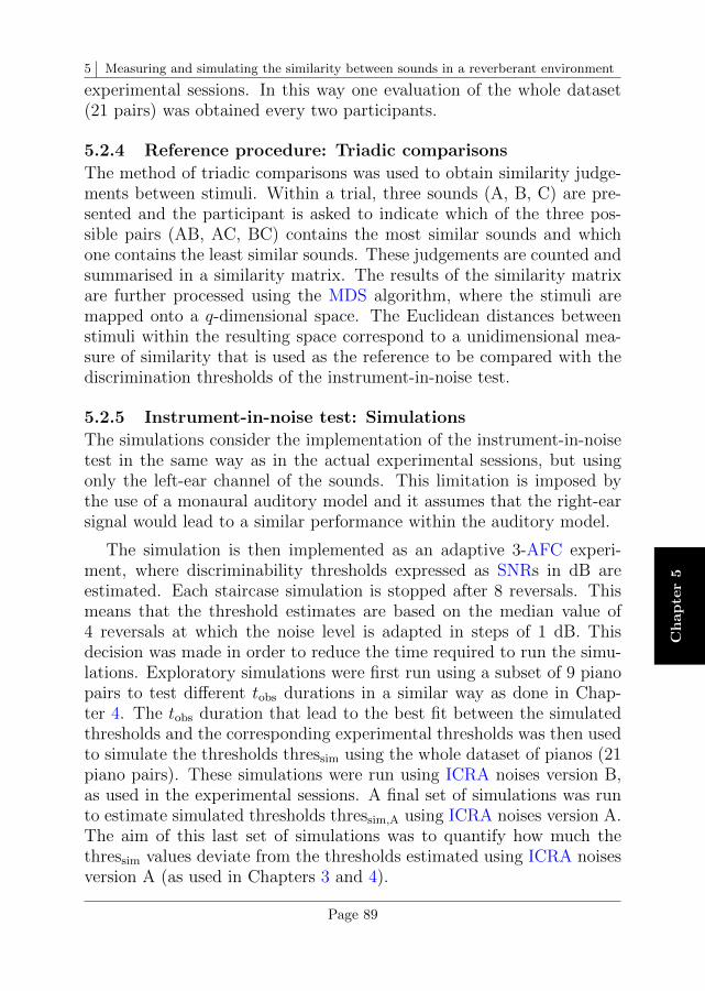
5 Measuring and simulating the similarity between sounds in a reverberant environment
Ch
ap
ter
5
experimental sessions. In this way one evaluation of the whole dataset(21 pairs) was obtained every two participants.
5.2.4 Reference procedure: Triadic comparisons
The method of triadic comparisons was used to obtain similarity judge-ments between stimuli. Within a trial, three sounds (A, B, C) are pre-sented and the participant is asked to indicate which of the three pos-sible pairs (AB, AC, BC) contains the most similar sounds and whichone contains the least similar sounds. These judgements are counted andsummarised in a similarity matrix. The results of the similarity matrixare further processed using the MDS algorithm, where the stimuli aremapped onto a q-dimensional space. The Euclidean distances betweenstimuli within the resulting space correspond to a unidimensional mea-sure of similarity that is used as the reference to be compared with thediscrimination thresholds of the instrument-in-noise test.
5.2.5 Instrument-in-noise test: Simulations
The simulations consider the implementation of the instrument-in-noisetest in the same way as in the actual experimental sessions, but usingonly the left-ear channel of the sounds. This limitation is imposed bythe use of a monaural auditory model and it assumes that the right-earsignal would lead to a similar performance within the auditory model.
The simulation is then implemented as an adaptive 3-AFC experi-ment, where discriminability thresholds expressed as SNRs in dB areestimated. Each staircase simulation is stopped after 8 reversals. Thismeans that the threshold estimates are based on the median value of4 reversals at which the noise level is adapted in steps of 1 dB. Thisdecision was made in order to reduce the time required to run the simu-lations. Exploratory simulations were first run using a subset of 9 pianopairs to test different tobs durations in a similar way as done in Chap-ter 4. The tobs duration that lead to the best fit between the simulatedthresholds and the corresponding experimental thresholds was then usedto simulate the thresholds thressim using the whole dataset of pianos (21piano pairs). These simulations were run using ICRA noises version B,as used in the experimental sessions. A final set of simulations was runto estimate simulated thresholds thressim,A using ICRA noises version A.The aim of this last set of simulations was to quantify how much thethressim values deviate from the thresholds estimated using ICRA noisesversion A (as used in Chapters 3 and 4).
Page 89
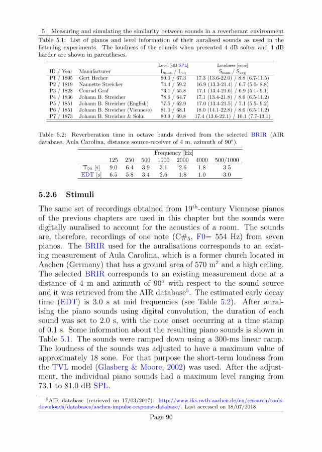
5 Measuring and simulating the similarity between sounds in a reverberant environment
Table 5.1: List of pianos and level information of their auralised sounds as used in thelistening experiments. The loudness of the sounds when presented 4 dB softer and 4 dBharder are shown in parentheses.
Level [dB SPL] Loudness [sone]
ID / Year Manufacturer Lmax / Leq Smax / Savg
P1 / 1805 Gert Hecher 80.0 / 67.3 17.3 (13.6-22.0) / 8.8 (6.7-11.5)P2 / 1819 Nannette Streicher 74.4 / 59.2 16.9 (13.3-21.4) / 6.7 (5.0- 8.8)P3 / 1828 Conrad Graf 73.1 / 55.8 17.1 (13.4-21.6) / 6.9 (5.1- 9.1)P4 / 1836 Johann B. Streicher 78.6 / 64.7 17.1 (13.4-21.8) / 8.6 (6.5-11.2)P5 / 1851 Johann B. Streicher (English) 77.5 / 62.9 17.0 (13.4-21.5) / 7.1 (5.5- 9.2)P6 / 1851 Johann B. Streicher (Viennese) 81.0 / 68.1 18.0 (14.1-22.8) / 8.6 (6.5-11.2)P7 / 1873 Johann B. Streicher & Sohn 80.9 / 69.8 17.4 (13.6-22.1) / 10.1 (7.7-13.1)
Table 5.2: Reverberation time in octave bands derived from the selected BRIR (AIRdatabase, Aula Carolina, distance source-receiver of 4 m, azimuth of 90o).
Frequency [Hz]125 250 500 1000 2000 4000 500/1000
T20 [s] 9.0 6.4 3.9 3.1 2.6 1.8 3.5EDT [s] 6.5 5.8 3.4 2.6 1.8 1.0 3.0
5.2.6 Stimuli
The same set of recordings obtained from 19th-century Viennese pianosof the previous chapters are used in this chapter but the sounds weredigitally auralised to account for the acoustics of a room. The soundsare, therefore, recordings of one note (C#5, F0= 554 Hz) from sevenpianos. The BRIR used for the auralisations corresponds to an exist-ing measurement of Aula Carolina, which is a former church located inAachen (Germany) that has a ground area of 570 m2 and a high ceiling.The selected BRIR corresponds to an existing measurement done at adistance of 4 m and azimuth of 90o with respect to the sound sourceand it was retrieved from the AIR database5. The estimated early decaytime (EDT) is 3.0 s at mid frequencies (see Table 5.2). After aural-ising the piano sounds using digital convolution, the duration of eachsound was set to 2.0 s, with the note onset occurring at a time stampof 0.1 s. Some information about the resulting piano sounds is shown inTable 5.1. The sounds were ramped down using a 300-ms linear ramp.The loudness of the sounds was adjusted to have a maximum value ofapproximately 18 sone. For that purpose the short-term loudness fromthe TVL model (Glasberg & Moore, 2002) was used. After the adjust-ment, the individual piano sounds had a maximum level ranging from73.1 to 81.0 dB SPL.
5AIR database (retrieved on 17/03/2017): http://www.iks.rwth-aachen.de/en/research/tools-downloads/databases/aachen-impulse-response-database/. Last accessed on 18/07/2018.
Page 90
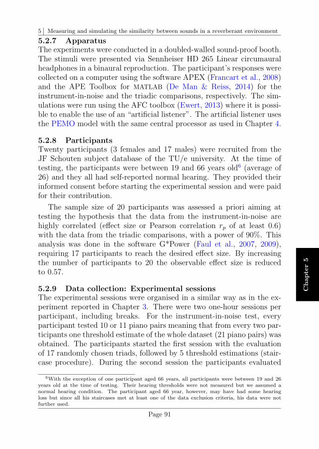
5 Measuring and simulating the similarity between sounds in a reverberant environment
Ch
ap
ter
5
5.2.7 ApparatusThe experiments were conducted in a doubled-walled sound-proof booth.The stimuli were presented via Sennheiser HD 265 Linear circumauralheadphones in a binaural reproduction. The participant’s responses werecollected on a computer using the software APEX (Francart et al., 2008)and the APE Toolbox for MATLAB (De Man & Reiss, 2014) for theinstrument-in-noise and the triadic comparisons, respectively. The sim-ulations were run using the AFC toolbox (Ewert, 2013) where it is possi-ble to enable the use of an “artificial listener”. The artificial listener usesthe PEMO model with the same central processor as used in Chapter 4.
5.2.8 ParticipantsTwenty participants (3 females and 17 males) were recruited from theJF Schouten subject database of the TU/e university. At the time oftesting, the participants were between 19 and 66 years old6 (average of26) and they all had self-reported normal hearing. They provided theirinformed consent before starting the experimental session and were paidfor their contribution.
The sample size of 20 participants was assessed a priori aiming attesting the hypothesis that the data from the instrument-in-noise arehighly correlated (effect size or Pearson correlation rp of at least 0.6)with the data from the triadic comparisons, with a power of 90%. Thisanalysis was done in the software G*Power (Faul et al., 2007, 2009),requiring 17 participants to reach the desired effect size. By increasingthe number of participants to 20 the observable effect size is reducedto 0.57.
5.2.9 Data collection: Experimental sessionsThe experimental sessions were organised in a similar way as in the ex-periment reported in Chapter 3. There were two one-hour sessions perparticipant, including breaks. For the instrument-in-noise test, everyparticipant tested 10 or 11 piano pairs meaning that from every two par-ticipants one threshold estimate of the whole dataset (21 piano pairs) wasobtained. The participants started the first session with the evaluationof 17 randomly chosen triads, followed by 5 threshold estimations (stair-case procedure). During the second session the participants evaluated
6With the exception of one participant aged 66 years, all participants were between 19 and 26years old at the time of testing. Their hearing thresholds were not measured but we assumed anormal hearing condition. The participant aged 66 year, however, may have had some hearingloss but since all his staircases met at least one of the data exclusion criteria, his data were notfurther used.
Page 91
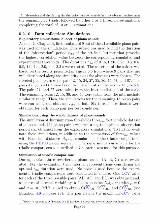
5 Measuring and simulating the similarity between sounds in a reverberant environment
the remaining 18 triads, followed by other 5 or 6 threshold estimations,completing the total of 10 or 11 estimations.
5.2.10 Data collection: SimulationsExploratory simulations: Subset of piano sounds
As done in Chapter 4, first a subset of 9 out of the 21 available piano pairswas used for the simulations. This subset was used to find the durationof the “observation” period tobs of the artificial listener that providesthe highest correlation value between the corresponding simulated andexperimental thresholds. The durations tobs of 0.16, 0.20, 0.25, 0.3, 0.5,0.8, 1.0, 1.4, 2.0, and 2.2 s were tested. The selection of the subset wasbased on the results presented in Figure 5.5 from where 9 pairs that arewell distributed along the similarity axis (the abscissa) were chosen. Theselected piano pairs were: pair 12, 15, 24, 27, 35, 36, 45, 47, and 67. Thepairs 47, 35, and 67 were taken from the most similar end of Figure 5.5.The pairs 24, and 27 were taken from the least similar end of the scale.The remaining pairs 12, 15, 36, and 45 were taken from the intermediatesimilarity range. Then, the simulations for the remaining 13 piano pairswere run using the obtained tobs period. Six threshold estimates wereobtained for each piano pair per test condition.
Simulations using the whole dataset of piano sounds
The simulation of discrimination thresholds thressim for the whole datasetof piano sounds (21 piano pairs) was run using the optimal observationperiod tobs obtained from the exploratory simulations. To further eval-uate these simulations, in addition to the comparison of thressim valueswith Euclidean distances dij exp, simulations of the triadic comparisonsusing the PEMO model were run. The same simulation scheme for thetriadic comparisons as described in Chapter 4 was used for this purpose.
Simulation of triadic comparisons
During a trial, three reverberant piano sounds (A, B, C) were evalu-ated. For the evaluation their internal representations considering theoptimal tobs duration were used. No noise is used because the experi-mental triadic comparisons were conducted in silence. One CCV valuefor each of the three possible pairs (AB, AC, and BC) was obtained and,as source of internal variability, a Gaussian noise Nx(µ, σ
2) with µ = 0
and σ = 10.1 MU7 is used to obtain CCVAB, CCVAC , and CCVBC (see
Equation 4.8 on page 70). The pair having the maximum CCV value
7Refer to Appendix D (Section D.3.3) for details about the internal noise configuration.
Page 92
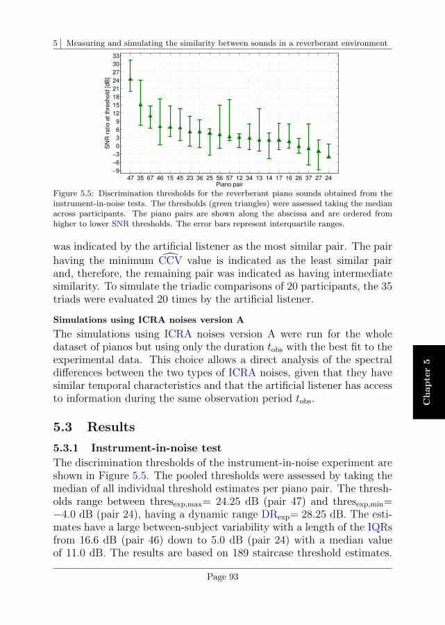
5 Measuring and simulating the similarity between sounds in a reverberant environment
Ch
ap
ter
5
47 35 67 46 15 45 23 36 25 56 57 12 34 13 14 17 16 26 37 27 24
−9
−6
−3
0
3
6
9
12
15
18
21
24
27
30
33
SN
R r
atio a
t th
reshold
[dB
]
Piano pair
Figure 5.5: Discrimination thresholds for the reverberant piano sounds obtained from theinstrument-in-noise tests. The thresholds (green triangles) were assessed taking the medianacross participants. The piano pairs are shown along the abscissa and are ordered fromhigher to lower SNR thresholds. The error bars represent interquartile ranges.
was indicated by the artificial listener as the most similar pair. The pair
having the minimum CCV value is indicated as the least similar pairand, therefore, the remaining pair was indicated as having intermediatesimilarity. To simulate the triadic comparisons of 20 participants, the 35triads were evaluated 20 times by the artificial listener.
Simulations using ICRA noises version A
The simulations using ICRA noises version A were run for the wholedataset of pianos but using only the duration tobs with the best fit to theexperimental data. This choice allows a direct analysis of the spectraldifferences between the two types of ICRA noises, given that they havesimilar temporal characteristics and that the artificial listener has accessto information during the same observation period tobs.
5.3 Results
5.3.1 Instrument-in-noise test
The discrimination thresholds of the instrument-in-noise experiment areshown in Figure 5.5. The pooled thresholds were assessed by taking themedian of all individual threshold estimates per piano pair. The thresh-olds range between thresexp,max= 24.25 dB (pair 47) and thresexp,min=−4.0 dB (pair 24), having a dynamic range DRexp= 28.25 dB. The esti-mates have a large between-subject variability with a length of the IQRsfrom 16.6 dB (pair 46) down to 5.0 dB (pair 24) with a median valueof 11.0 dB. The results are based on 189 staircase threshold estimates.
Page 93
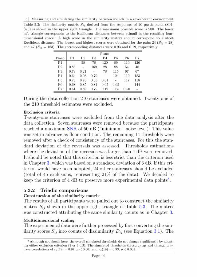
5 Measuring and simulating the similarity between sounds in a reverberant environment
Table 5.3: The similarity matrix Sij derived from the responses of 20 participants (S01-S20) is shown in the upper right triangle. The maximum possible score is 200. The lowerleft triangle corresponds to the Euclidean distances between stimuli in the resulting four-dimensional space. A high score in the similarity matrix should correspond to a shortEuclidean distance. The lowest and highest scores were obtained for the pairs 24 (Sij = 28)and 47 (Sij = 183). The corresponding distances were 0.93 and 0.19, respectively.
Piano
Piano P1 P2 P3 P4 P5 P6 P7P1 - 58 78 120 89 110 126P2 0.85 - 169 28 88 54 48P3 0.78 0.21 - 78 115 67 67P4 0.64 0.93 0.79 - 124 119 183P5 0.76 0.78 0.65 0.61 - 117 118P6 0.68 0.85 0.84 0.65 0.65 - 144P7 0.61 0.89 0.79 0.19 0.65 0.50 -
During the data collection 210 staircases were obtained. Twenty-one ofthe 210 threshold estimates were excluded.
Exclusion criteria
Twenty-one staircases were excluded from the data analysis after thedata collection. Seven staircases were removed because the participantsreached a maximum SNR of 50 dB (“minimum” noise level). This valuewas set in advance as floor condition. The remaining 14 thresholds wereremoved after a check of consistency of the staircases. For this the stan-dard deviation of the reversals was assessed. Thresholds estimationswhere the deviation of the reversals was larger than 4 dB were removed.It should be noted that this criterion is less strict than the criterion usedin Chapter 3, which was based on a standard deviation of 3 dB. If this cri-terion would have been adopted, 24 other staircases should be excluded(total of 45 exclusions, representing 21% of the data). We decided tokeep the criterion of 4 dB to preserve more experimental data points8.
5.3.2 Triadic comparisonsConstruction of the similarity matrix
The results of all participants were pulled out to construct the similaritymatrix Sij shown in the upper right triangle of Table 5.3. The matrixwas constructed attributing the same similarity counts as in Chapter 3.
Multidimensional scaling
The experimental data were further processed by first converting the sim-ilarity scores Sij into counts of dissimilarity Dij (see Equation 3.1). The
8Although not shown here, the overall simulated thresholds do not change significantly by adopt-ing either exclusion criterion (3 or 4 dB). The simulated thresholds thressim,3 dB and thressim,4 dB
have correlations of rp(19) = 0.97, p < 0.001 and rs(19) = 0.93, p < 0.001.
Page 94
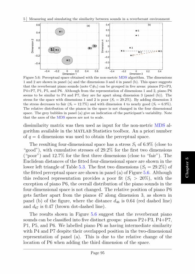
5 Measuring and simulating the similarity between sounds in a reverberant environment
Ch
ap
ter
5
−0.4 −0.2 0 0.2 0.4 0.6
−0.4
−0.2
0
0.2
0.4
0.6
1
23
5
647
Dimension 1
Dim
ensio
n 2
(a)
−0.4 −0.2 0 0.2 0.4
−0.4
−0.3
−0.2
−0.1
0
0.1
0.2
0.3
0.4
1
2
3
4
5
6
7
Dimension 3
Dim
ensio
n 4
(b)
Figure 5.6: Perceptual space obtained with the non-metric MDS algorithm. The dimensions1 and 2 are shown in panel (a) and the dimensions 3 and 4 in panel (b). This space suggeststhat the reverberant piano sounds (note C#5) can be grouped in five areas: pianos P2+P3,P4+P7, P1, P5, and P6. Although from the representation of dimensions 1 and 2, piano P6seems to be similar to P4 and P7, they are far apart along dimension 3 (panel (b)). Thestress for the space with dimensions 1 and 2 is poor (St = 29.2%). By adding dimension 3the stress decreases to fair (St = 12.7%) and with dimension 4 to nearly good (St = 6.9%).The relative distribution of the pianos in the space is not changed in the four dimensionalspace. The grey bubbles in panel (a) give an indication of the participant’s variability. Notethat the axes of the MDS spaces are not to scale.
dissimilarity matrix was then used as input for the non-metric MDS al-gorithm available in the MATLAB Statistics toolbox. An a priori numberof q = 4 dimensions was used to obtain the perceptual space.
The resulting four-dimensional space has a stress St of 6.9% (close to“good”), with cumulative stresses of 29.2% for the first two dimensions(“poor”) and 12.7% for the first three dimensions (close to “fair”). TheEuclidean distances of the fitted four-dimensional space are shown in thelower left triangle of Table 5.3. The first two dimensions (St = 29.2%) ofthe fitted perceptual space are shown in panel (a) of Figure 5.6. Althoughthis reduced representation provides a poor fit (St > 20%), with theexception of piano P6, the overall distribution of the piano sounds in thefour-dimensional space is not changed. The relative position of piano P6gets farther apart from the pianos 47 along dimension 3, as shown inpanel (b) of the figure, where the distance d46 is 0.64 (red dashed line)and d67 is 0.47 (brown dot-dashed line).
The results shown in Figure 5.6 suggest that the reverberant pianosounds can be classified into five distinct groups: pianos P2+P3, P4+P7,P1, P5, and P6. We labelled piano P6 as having intermediate similaritywith P4 and P7 despite their overlapped position in the two-dimensionalrepresentation of panel (a). This is due to the relative change of thelocation of P6 when adding the third dimension of the space.
Page 95
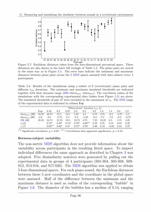
5 Measuring and simulating the similarity between sounds in a reverberant environment
47 35 67 46 15 45 23 36 25 56 57 12 34 13 14 17 16 26 37 27 24
0.1
0.2
0.3
0.4
0.5
0.6
0.7
0.8
0.9
Eu
clid
ea
n d
ista
nce
Piano pair
Figure 5.7: Euclidean distances taken from the four-dimensional perceptual space. Thesedistances are also shown in the lower left triangle of Table 5.3. The piano pairs are sortedin the same way as in Figure 5.5. The error bars indicate the minimum and maximumdistances between piano pairs across the 5 MDS spaces assessed with data subsets every 4participants.
Table 5.4: Results of the simulations using a subset of 9 (reverberant) piano pairs anddifferent tobs durations. The minimum and maximum simulated thresholds are indicatedtogether with their dynamic range (DR=thresmax−thresmin). The correlation values of thesimulations with the corresponding experimental data (taken from Figure 5.5) are given.The simulated thresholds of pair 47 were excluded in the assessment of rp. The SNR rangeof the experimental data is indicated in column Exp.
“Observation” duration tobs [s]Exp. 0.16 0.2 0.25 0.3 0.5 0.8 1.0 1.4 2.0 2.2
thresmax [dB] 24.25 20.75 15.5 13.5 5.25 4.5 0.75 2.75 -0.5 -2.75 -5.5thresmin [dB] -4.0 -4.0 -5.75 -5.5 -5.5 -5.25 -6.5 -7.5 -7.0 -8.5 -9.75DR [dB] 28.25 24.75 21.25 19.0 10.75 9.75 7.25 10.25 6.5 5.75 4.25rp(6) – 0.73* 0.88* 0.74* 0.76* 0.60** 0.42 0.25 0.19 0.25 0.28rs(7) – 0.63** 0.80* 0.57 0.75* 0.76* 0.36 0.19 -0.02 0.24 0.37
(*) Significant correlation, p < 0.05. (**) Correlations that approach significance, p < 0.10.
Between-subject variability
The non-metric MDS algorithm does not provide information about thevariability across participants in the resulting fitted space. To inspectindividual differences the same approach as described in Chapter 3 wasadopted. Five dissimilarity matrices were generated by pulling out theexperimental data in groups of 4 participants (S01-S04, S05-S08, S09-S12, S13-S16, and S17-S20). The MDS algorithm was applied to obtain5 four-dimensional spaces. For each piano sound, the Euclidean distancesbetween these 5 new coordinates and the coordinate in the global spacewere assessed. Half of the difference between the minimum and themaximum distance is used as radius of the corresponding “bubble” inFigure 5.6. The diameter of the bubbles has a median of 0.14, ranging
Page 96
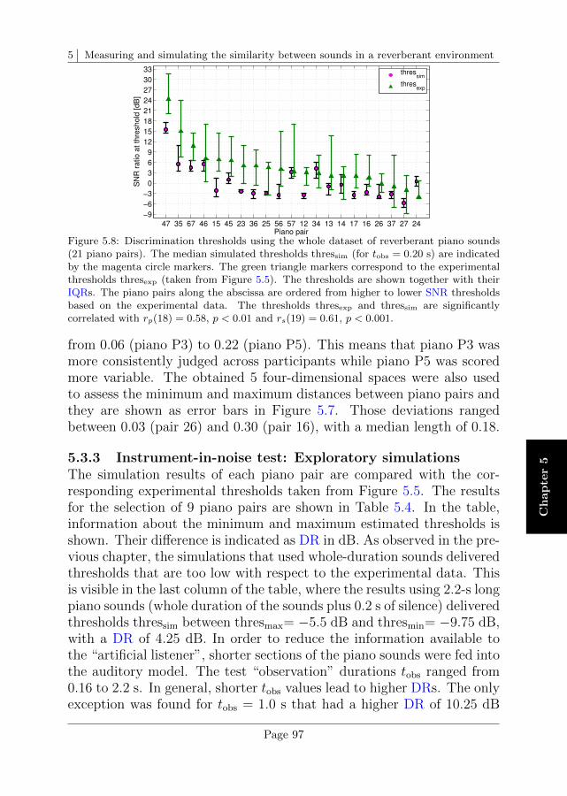
5 Measuring and simulating the similarity between sounds in a reverberant environment
Ch
ap
ter
5
47 35 67 46 15 45 23 36 25 56 57 12 34 13 14 17 16 26 37 27 24
−9
−6
−3
0
3
6
9
12
15
18
21
24
27
30
33
Full dataset, 0.20−s
Piano pair
SN
R r
atio a
t th
reshold
[dB
]
thressim
thresexp
Figure 5.8: Discrimination thresholds using the whole dataset of reverberant piano sounds(21 piano pairs). The median simulated thresholds thressim (for tobs = 0.20 s) are indicatedby the magenta circle markers. The green triangle markers correspond to the experimentalthresholds thresexp (taken from Figure 5.5). The thresholds are shown together with theirIQRs. The piano pairs along the abscissa are ordered from higher to lower SNR thresholdsbased on the experimental data. The thresholds thresexp and thressim are significantlycorrelated with rp(18) = 0.58, p < 0.01 and rs(19) = 0.61, p < 0.001.
from 0.06 (piano P3) to 0.22 (piano P5). This means that piano P3 wasmore consistently judged across participants while piano P5 was scoredmore variable. The obtained 5 four-dimensional spaces were also usedto assess the minimum and maximum distances between piano pairs andthey are shown as error bars in Figure 5.7. Those deviations rangedbetween 0.03 (pair 26) and 0.30 (pair 16), with a median length of 0.18.
5.3.3 Instrument-in-noise test: Exploratory simulationsThe simulation results of each piano pair are compared with the cor-responding experimental thresholds taken from Figure 5.5. The resultsfor the selection of 9 piano pairs are shown in Table 5.4. In the table,information about the minimum and maximum estimated thresholds isshown. Their difference is indicated as DR in dB. As observed in the pre-vious chapter, the simulations that used whole-duration sounds deliveredthresholds that are too low with respect to the experimental data. Thisis visible in the last column of the table, where the results using 2.2-s longpiano sounds (whole duration of the sounds plus 0.2 s of silence) deliveredthresholds thressim between thresmax= −5.5 dB and thresmin= −9.75 dB,with a DR of 4.25 dB. In order to reduce the information available tothe “artificial listener”, shorter sections of the piano sounds were fed intothe auditory model. The test “observation” durations tobs ranged from0.16 to 2.2 s. In general, shorter tobs values lead to higher DRs. The onlyexception was found for tobs = 1.0 s that had a higher DR of 10.25 dB
Page 97
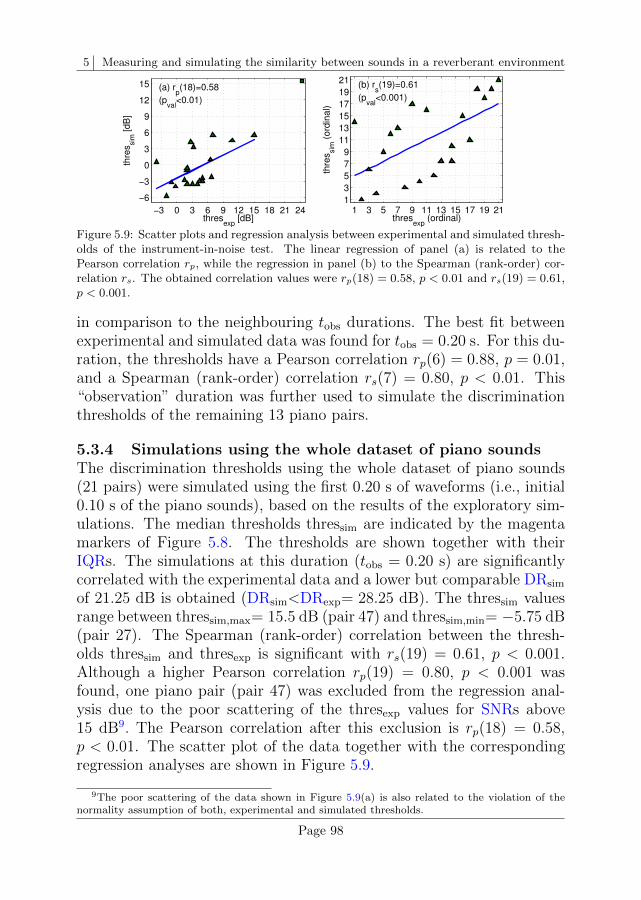
5 Measuring and simulating the similarity between sounds in a reverberant environment
−3 0 3 6 9 12 15 18 21 24
−6
−3
0
3
6
9
12
15
thresexp
[dB]
thre
ssim
[dB
]
Regression analysis / Full dataset, 0.20−s
(a) rp(18)=0.58
(pval
<0.01)
1 3 5 7 9 11 13 15 17 19 211
3
5
7
9
11
13
15
17
19
21
thresexp
(ordinal)
thre
ssim
(ord
inal)
Regression analysis / Full dataset, 0.20−s
(b) rs(19)=0.61
(pval
<0.001)
Figure 5.9: Scatter plots and regression analysis between experimental and simulated thresh-olds of the instrument-in-noise test. The linear regression of panel (a) is related to thePearson correlation rp, while the regression in panel (b) to the Spearman (rank-order) cor-relation rs. The obtained correlation values were rp(18) = 0.58, p < 0.01 and rs(19) = 0.61,p < 0.001.
in comparison to the neighbouring tobs durations. The best fit betweenexperimental and simulated data was found for tobs = 0.20 s. For this du-ration, the thresholds have a Pearson correlation rp(6) = 0.88, p = 0.01,and a Spearman (rank-order) correlation rs(7) = 0.80, p < 0.01. This“observation” duration was further used to simulate the discriminationthresholds of the remaining 13 piano pairs.
5.3.4 Simulations using the whole dataset of piano soundsThe discrimination thresholds using the whole dataset of piano sounds(21 pairs) were simulated using the first 0.20 s of waveforms (i.e., initial0.10 s of the piano sounds), based on the results of the exploratory sim-ulations. The median thresholds thressim are indicated by the magentamarkers of Figure 5.8. The thresholds are shown together with theirIQRs. The simulations at this duration (tobs = 0.20 s) are significantlycorrelated with the experimental data and a lower but comparable DRsim
of 21.25 dB is obtained (DRsim<DRexp= 28.25 dB). The thressim valuesrange between thressim,max= 15.5 dB (pair 47) and thressim,min= −5.75 dB(pair 27). The Spearman (rank-order) correlation between the thresh-olds thressim and thresexp is significant with rs(19) = 0.61, p < 0.001.Although a higher Pearson correlation rp(19) = 0.80, p < 0.001 wasfound, one piano pair (pair 47) was excluded from the regression anal-ysis due to the poor scattering of the thresexp values for SNRs above15 dB9. The Pearson correlation after this exclusion is rp(18) = 0.58,p < 0.01. The scatter plot of the data together with the correspondingregression analyses are shown in Figure 5.9.
9The poor scattering of the data shown in Figure 5.9(a) is also related to the violation of thenormality assumption of both, experimental and simulated thresholds.
Page 98
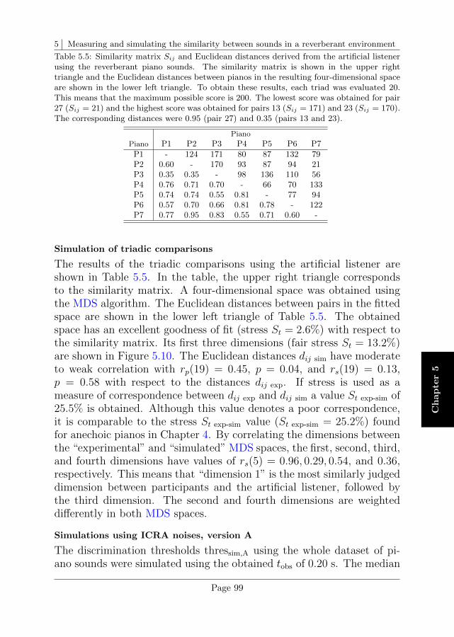
5 Measuring and simulating the similarity between sounds in a reverberant environment
Ch
ap
ter
5
Table 5.5: Similarity matrix Sij and Euclidean distances derived from the artificial listenerusing the reverberant piano sounds. The similarity matrix is shown in the upper righttriangle and the Euclidean distances between pianos in the resulting four-dimensional spaceare shown in the lower left triangle. To obtain these results, each triad was evaluated 20.This means that the maximum possible score is 200. The lowest score was obtained for pair27 (Sij = 21) and the highest score was obtained for pairs 13 (Sij = 171) and 23 (Sij = 170).The corresponding distances were 0.95 (pair 27) and 0.35 (pairs 13 and 23).
Piano
Piano P1 P2 P3 P4 P5 P6 P7P1 - 124 171 80 87 132 79P2 0.60 - 170 93 87 94 21P3 0.35 0.35 - 98 136 110 56P4 0.76 0.71 0.70 - 66 70 133P5 0.74 0.74 0.55 0.81 - 77 94P6 0.57 0.70 0.66 0.81 0.78 - 122P7 0.77 0.95 0.83 0.55 0.71 0.60 -
Simulation of triadic comparisons
The results of the triadic comparisons using the artificial listener areshown in Table 5.5. In the table, the upper right triangle correspondsto the similarity matrix. A four-dimensional space was obtained usingthe MDS algorithm. The Euclidean distances between pairs in the fittedspace are shown in the lower left triangle of Table 5.5. The obtainedspace has an excellent goodness of fit (stress St = 2.6%) with respect tothe similarity matrix. Its first three dimensions (fair stress St = 13.2%)are shown in Figure 5.10. The Euclidean distances dij sim have moderateto weak correlation with rp(19) = 0.45, p = 0.04, and rs(19) = 0.13,p = 0.58 with respect to the distances dij exp. If stress is used as ameasure of correspondence between dij exp and dij sim a value St exp-sim of25.5% is obtained. Although this value denotes a poor correspondence,it is comparable to the stress St exp-sim value (St exp-sim = 25.2%) foundfor anechoic pianos in Chapter 4. By correlating the dimensions betweenthe “experimental” and “simulated” MDS spaces, the first, second, third,and fourth dimensions have values of rs(5) = 0.96, 0.29, 0.54, and 0.36,respectively. This means that “dimension 1” is the most similarly judgeddimension between participants and the artificial listener, followed bythe third dimension. The second and fourth dimensions are weighteddifferently in both MDS spaces.
Simulations using ICRA noises, version A
The discrimination thresholds thressim,A using the whole dataset of pi-ano sounds were simulated using the obtained tobs of 0.20 s. The median
Page 99
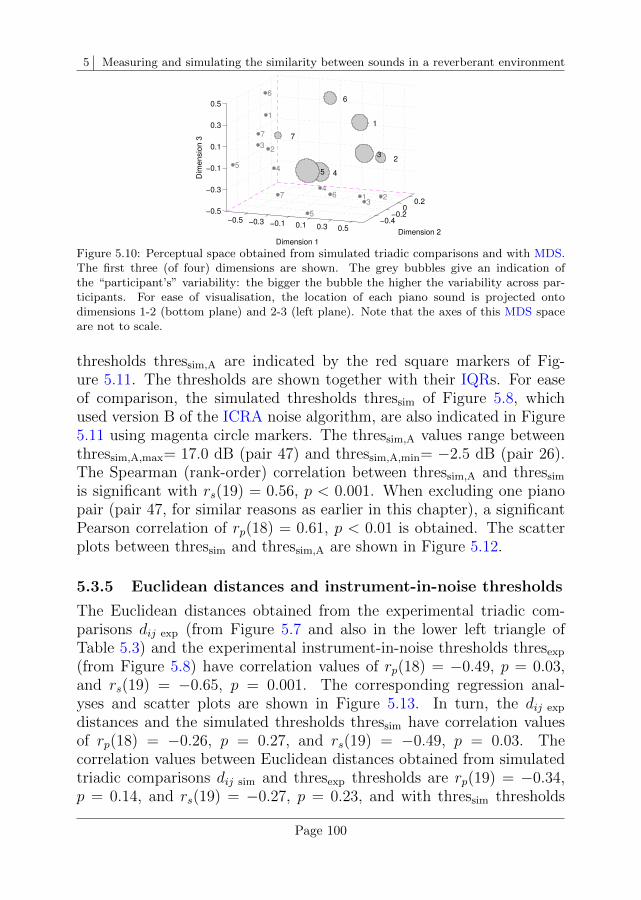
5 Measuring and simulating the similarity between sounds in a reverberant environment
−0.5 −0.3 −0.1 0.1 0.3 0.5−0.4
−0.20
0.2
−0.5
−0.3
−0.1
0.1
0.3
0.5
Dimension 2
2
2
3
1
31
6
4
64
5
Dimension 1
5
7
7
4
2
1
6
7
3
5
Dim
ensio
n 3
Figure 5.10: Perceptual space obtained from simulated triadic comparisons and with MDS.The first three (of four) dimensions are shown. The grey bubbles give an indication ofthe “participant’s” variability: the bigger the bubble the higher the variability across par-ticipants. For ease of visualisation, the location of each piano sound is projected ontodimensions 1-2 (bottom plane) and 2-3 (left plane). Note that the axes of this MDS spaceare not to scale.
thresholds thressim,A are indicated by the red square markers of Fig-ure 5.11. The thresholds are shown together with their IQRs. For easeof comparison, the simulated thresholds thressim of Figure 5.8, whichused version B of the ICRA noise algorithm, are also indicated in Figure5.11 using magenta circle markers. The thressim,A values range betweenthressim,A,max= 17.0 dB (pair 47) and thressim,A,min= −2.5 dB (pair 26).The Spearman (rank-order) correlation between thressim,A and thressim
is significant with rs(19) = 0.56, p < 0.001. When excluding one pianopair (pair 47, for similar reasons as earlier in this chapter), a significantPearson correlation of rp(18) = 0.61, p < 0.01 is obtained. The scatterplots between thressim and thressim,A are shown in Figure 5.12.
5.3.5 Euclidean distances and instrument-in-noise thresholds
The Euclidean distances obtained from the experimental triadic com-parisons dij exp (from Figure 5.7 and also in the lower left triangle ofTable 5.3) and the experimental instrument-in-noise thresholds thresexp
(from Figure 5.8) have correlation values of rp(18) = −0.49, p = 0.03,and rs(19) = −0.65, p = 0.001. The corresponding regression anal-yses and scatter plots are shown in Figure 5.13. In turn, the dij exp
distances and the simulated thresholds thressim have correlation valuesof rp(18) = −0.26, p = 0.27, and rs(19) = −0.49, p = 0.03. Thecorrelation values between Euclidean distances obtained from simulatedtriadic comparisons dij sim and thresexp thresholds are rp(19) = −0.34,p = 0.14, and rs(19) = −0.27, p = 0.23, and with thressim thresholds
Page 100
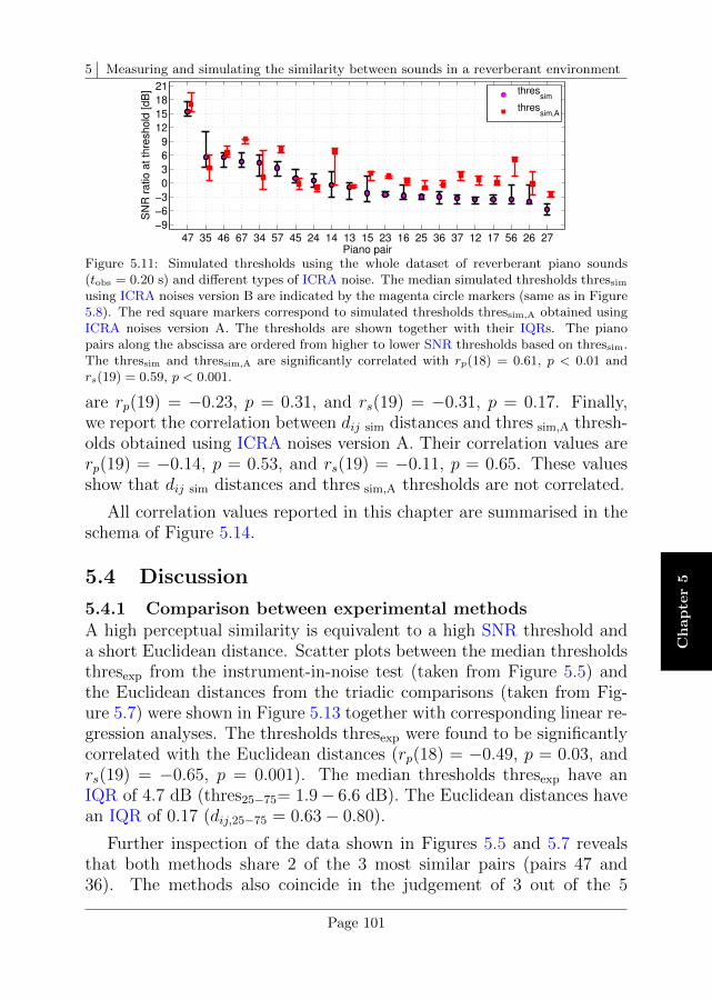
5 Measuring and simulating the similarity between sounds in a reverberant environment
Ch
ap
ter
5
47 35 46 67 34 57 45 24 14 13 15 23 16 25 36 37 12 17 56 26 27−9
−6
−3
0
3
6
9
12
15
18
21
Full dataset, 0.20−s
Piano pair
SN
R r
atio
at
thre
sh
old
[d
B]
thressim
thressim,A
Figure 5.11: Simulated thresholds using the whole dataset of reverberant piano sounds(tobs = 0.20 s) and different types of ICRA noise. The median simulated thresholds thressim
using ICRA noises version B are indicated by the magenta circle markers (same as in Figure5.8). The red square markers correspond to simulated thresholds thressim,A obtained usingICRA noises version A. The thresholds are shown together with their IQRs. The pianopairs along the abscissa are ordered from higher to lower SNR thresholds based on thressim.The thressim and thressim,A are significantly correlated with rp(18) = 0.61, p < 0.01 andrs(19) = 0.59, p < 0.001.
are rp(19) = −0.23, p = 0.31, and rs(19) = −0.31, p = 0.17. Finally,we report the correlation between dij sim distances and thres sim,A thresh-olds obtained using ICRA noises version A. Their correlation values arerp(19) = −0.14, p = 0.53, and rs(19) = −0.11, p = 0.65. These valuesshow that dij sim distances and thres sim,A thresholds are not correlated.
All correlation values reported in this chapter are summarised in theschema of Figure 5.14.
5.4 Discussion
5.4.1 Comparison between experimental methodsA high perceptual similarity is equivalent to a high SNR threshold anda short Euclidean distance. Scatter plots between the median thresholdsthresexp from the instrument-in-noise test (taken from Figure 5.5) andthe Euclidean distances from the triadic comparisons (taken from Fig-ure 5.7) were shown in Figure 5.13 together with corresponding linear re-gression analyses. The thresholds thresexp were found to be significantlycorrelated with the Euclidean distances (rp(18) = −0.49, p = 0.03, andrs(19) = −0.65, p = 0.001). The median thresholds thresexp have anIQR of 4.7 dB (thres25−75= 1.9− 6.6 dB). The Euclidean distances havean IQR of 0.17 (dij,25−75 = 0.63− 0.80).
Further inspection of the data shown in Figures 5.5 and 5.7 revealsthat both methods share 2 of the 3 most similar pairs (pairs 47 and36). The methods also coincide in the judgement of 3 out of the 5
Page 101

5 Measuring and simulating the similarity between sounds in a reverberant environment
−4 −2 0 2 4 6−4
−2
0
2
4
6
8
10
12
thressim
[dB]
thre
ssim
,A [
dB
]
Regression analysis / Full dataset, 0.20−s
(a) rp(18)=0.61
(pval
<0.01)
1 3 5 7 9 11 13 15 17 19 211
3
5
7
9
11
13
15
17
19
21
thressim
(ordinal)
thre
ssim
,A (
ord
ina
l)
Regression analysis / Full dataset, 0.20−s
(b) rs(19)=0.56
(pval
<0.001)
Figure 5.12: Scatter plots and regression analysis between simulated thresholds using dif-ferent types of ICRA noise. The linear regression of panel (a) is related to the Pearsoncorrelation rp, while the regression in panel (b) to the Spearman (rank-order) correlationrs. One pair of points was removed from the analysis to obtain an rp(18) = 0.61, p < 0.01,due to the lack of thressim values above 6 dB. A Spearman correlation of rs(19) = 0.59,p < 0.001 is obtained.
−3 0 3 6 9 12 15 18 21 24
0.1
0.2
0.3
0.4
0.5
0.6
0.7
0.8
0.9
SNR at threshold, thresexp
[dB]
Euclid
ean d
ista
nce
Regression analysis − Pearson
(a) rp(18)=−0.49
(pval
=0.03)
1 3 5 7 9 11 13 15 17 19 211
3
5
7
9
11
13
15
17
19
21
SNR at threshold, thresexp
(ordinal)
Euclid
ean d
ista
nce (
ord
inal)
Regression analysis − Spearman
(b) rs(19)=−0.65
(pval
=0.001)
Figure 5.13: Scatter plots and regression analysis between the results of the instrument-in-noise (SNR thresholds, thresexp) and triadic comparisons tests (Euclidean distances). Thelinear regression of panel (a) is related to the Pearson correlation rp, while the regressionin panel (b) to the Spearman (rank-order) correlation rs. One pair of points was removedfrom the analysis to obtain an rp(18) = −0.49, p = 0.03, due to the lack of thresexp valuesabove 15 dB. A Spearman correlation of rs(19) = −0.65, p = 0.001.
Figure 5.14: Summary of correlation values between instrument-in-noise thresholds andEuclidean distances. All possible combinations among thresexp, thressim, dij exp, and dij exp
are indicated in this schema. The correlation values of the simulated thresholds using theICRA noise algorithm version A with thressim and dij sim are also indicated.
Page 102
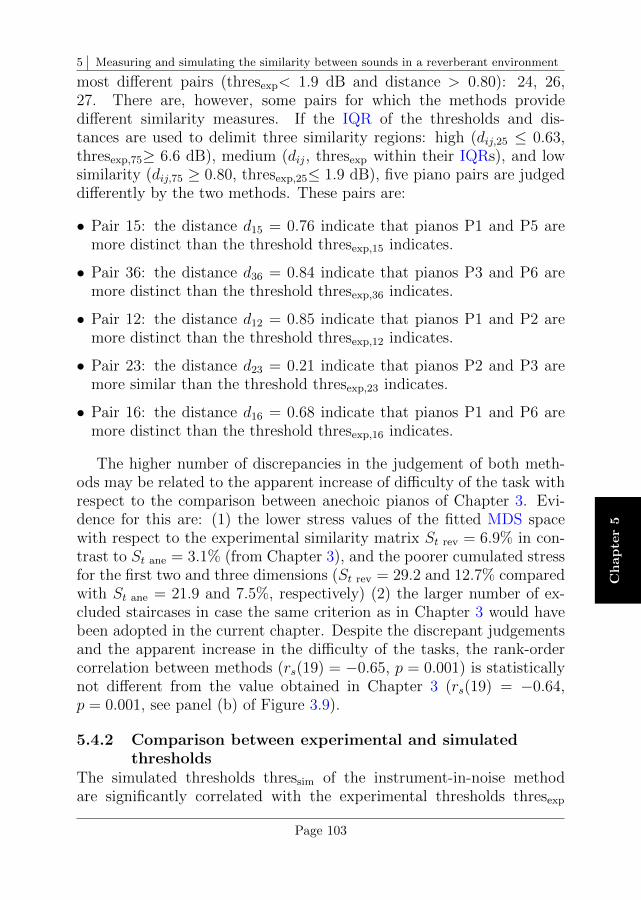
5 Measuring and simulating the similarity between sounds in a reverberant environment
Ch
ap
ter
5
most different pairs (thresexp< 1.9 dB and distance > 0.80): 24, 26,27. There are, however, some pairs for which the methods providedifferent similarity measures. If the IQR of the thresholds and dis-tances are used to delimit three similarity regions: high (dij,25 ≤ 0.63,thresexp,75≥ 6.6 dB), medium (dij, thresexp within their IQRs), and lowsimilarity (dij,75 ≥ 0.80, thresexp,25≤ 1.9 dB), five piano pairs are judgeddifferently by the two methods. These pairs are:
• Pair 15: the distance d15 = 0.76 indicate that pianos P1 and P5 aremore distinct than the threshold thresexp,15 indicates.
• Pair 36: the distance d36 = 0.84 indicate that pianos P3 and P6 aremore distinct than the threshold thresexp,36 indicates.
• Pair 12: the distance d12 = 0.85 indicate that pianos P1 and P2 aremore distinct than the threshold thresexp,12 indicates.
• Pair 23: the distance d23 = 0.21 indicate that pianos P2 and P3 aremore similar than the threshold thresexp,23 indicates.
• Pair 16: the distance d16 = 0.68 indicate that pianos P1 and P6 aremore distinct than the threshold thresexp,16 indicates.
The higher number of discrepancies in the judgement of both meth-ods may be related to the apparent increase of difficulty of the task withrespect to the comparison between anechoic pianos of Chapter 3. Evi-dence for this are: (1) the lower stress values of the fitted MDS spacewith respect to the experimental similarity matrix St rev = 6.9% in con-trast to St ane = 3.1% (from Chapter 3), and the poorer cumulated stressfor the first two and three dimensions (St rev = 29.2 and 12.7% comparedwith St ane = 21.9 and 7.5%, respectively) (2) the larger number of ex-cluded staircases in case the same criterion as in Chapter 3 would havebeen adopted in the current chapter. Despite the discrepant judgementsand the apparent increase in the difficulty of the tasks, the rank-ordercorrelation between methods (rs(19) = −0.65, p = 0.001) is statisticallynot different from the value obtained in Chapter 3 (rs(19) = −0.64,p = 0.001, see panel (b) of Figure 3.9).
5.4.2 Comparison between experimental and simulatedthresholds
The simulated thresholds thressim of the instrument-in-noise methodare significantly correlated with the experimental thresholds thresexp
Page 103
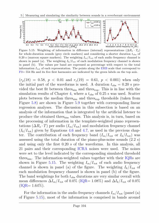
5 Measuring and simulating the similarity between sounds in a reverberant environment
3.4 5.4 7.4 9.4 11.4 13.4 15.4 17.4 19.4 21.4 23.4 25.4 27.4 29.4 31.4
02468
101214161820
Audio centre frequency fc [ERB
N]
Perc
enta
ge [%
]
(a) tobs
=0.20 s
tobs
=2.20 s
554 1108 1662 2216 2770 3324 [Hz]
1 2 3 4 5 6 7 8 9 10 11 12
02468
101214161820
Pe
rce
nta
ge
[%
]
Modulation centre frequency mfc [Nr.]
(b)
Figure 5.15: Weighting of information in difference (internal) representations (∆Rx · Tp)for whole-duration sounds (grey circle markers) and considering a shorter duration tobs of0.20 s (maroon square markers). The weighting Im/Itot of each audio frequency channel isshown in panel (a). The weighting Ik/Itot of each modulation frequency channel is shownin panel (b). The values per band are expressed as percentage with respect to the totalinformation Itot of each representation. The points along the ERB scale that correspond toF0= 554 Hz and its five first harmonics are indicated by the green labels on the top axis.
(rp(18) = 0.58, p < 0.01 and rs(19) = 0.61, p < 0.001) when onlythe initial part of the waveforms is used. A duration tobs = 0.20 s pro-vided the best fit between thressim and thresexp. This is in line with thesimulation results of Chapter 4, where a tobs of 0.25 s was used. Scatterplots between the median thressim and thresexp thresholds (taken fromFigure 5.8) are shown in Figure 5.9 together with corresponding linearregression analyses. The discussion in this subsection is based on ananalysis of the information that is integrated by the artificial listener toproduce the obtained thressim values. This analysis is, in turn, based onthe processing of information in the template-weighted piano represen-tations (∆Rx ·T ) per audio (Im/Itot) and modulation frequency channel(Ik/Itot) given by Equations 4.6 and 4.7, as used in the previous chap-ter. The contribution of each frequency band (Im/Itot or Ik/Itot) wasassessed using the total duration of the piano-plus-noise sounds (2.2 s)and using only the first 0.20 s of the waveforms. In this analysis, all21 pairs and their corresponding ICRA noises were used. The noiseswere set to the level indicated by the corresponding simulated thresholdthressim. The information-weighted values together with their IQRs areshown in Figure 5.15. The weighting Im/Itot of each audio frequencychannel is shown in panel (a) of the figure. The weighting Ik/Itot ofeach modulation frequency channel is shown in panel (b) of the figure.The band weightings for both tobs durations are very similar overall withmean differences ∆Im/Itot of 0.0% (IQR= 1.08%) and ∆Ik/Itot of 0.0%(IQR= 1.64%).
For the information in the audio frequency channels Im/Itot (panel (a)of Figure 5.15), most of the information is comprised in bands around
Page 104
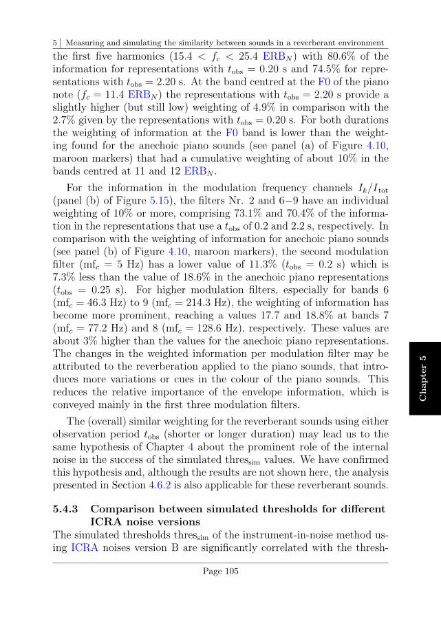
5 Measuring and simulating the similarity between sounds in a reverberant environment
Ch
ap
ter
5
the first five harmonics (15.4 < fc < 25.4 ERBN) with 80.6% of theinformation for representations with tobs = 0.20 s and 74.5% for repre-sentations with tobs = 2.20 s. At the band centred at the F0 of the pianonote (fc = 11.4 ERBN) the representations with tobs = 2.20 s provide aslightly higher (but still low) weighting of 4.9% in comparison with the2.7% given by the representations with tobs = 0.20 s. For both durationsthe weighting of information at the F0 band is lower than the weight-ing found for the anechoic piano sounds (see panel (a) of Figure 4.10,maroon markers) that had a cumulative weighting of about 10% in thebands centred at 11 and 12 ERBN .
For the information in the modulation frequency channels Ik/Itot
(panel (b) of Figure 5.15), the filters Nr. 2 and 6−9 have an individualweighting of 10% or more, comprising 73.1% and 70.4% of the informa-tion in the representations that use a tobs of 0.2 and 2.2 s, respectively. Incomparison with the weighting of information for anechoic piano sounds(see panel (b) of Figure 4.10, maroon markers), the second modulationfilter (mfc = 5 Hz) has a lower value of 11.3% (tobs = 0.2 s) which is7.3% less than the value of 18.6% in the anechoic piano representations(tobs = 0.25 s). For higher modulation filters, especially for bands 6(mfc = 46.3 Hz) to 9 (mfc = 214.3 Hz), the weighting of information hasbecome more prominent, reaching a values 17.7 and 18.8% at bands 7(mfc = 77.2 Hz) and 8 (mfc = 128.6 Hz), respectively. These values areabout 3% higher than the values for the anechoic piano representations.The changes in the weighted information per modulation filter may beattributed to the reverberation applied to the piano sounds, that intro-duces more variations or cues in the colour of the piano sounds. Thisreduces the relative importance of the envelope information, which isconveyed mainly in the first three modulation filters.
The (overall) similar weighting for the reverberant sounds using eitherobservation period tobs (shorter or longer duration) may lead us to thesame hypothesis of Chapter 4 about the prominent role of the internalnoise in the success of the simulated thressim values. We have confirmedthis hypothesis and, although the results are not shown here, the analysispresented in Section 4.6.2 is also applicable for these reverberant sounds.
5.4.3 Comparison between simulated thresholds for differentICRA noise versions
The simulated thresholds thressim of the instrument-in-noise method us-ing ICRA noises version B are significantly correlated with the thresh-
Page 105
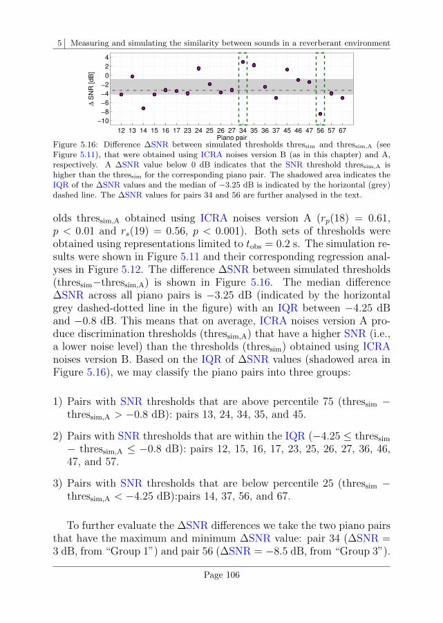
5 Measuring and simulating the similarity between sounds in a reverberant environment
12 13 14 15 16 17 23 24 25 26 27 34 35 36 37 45 46 47 56 57 67
−10
−8
−6
−4
−2
0
2
4
Piano pair
∆ S
NR
[d
B]
Figure 5.16: Difference ∆SNR between simulated thresholds thressim and thressim,A (seeFigure 5.11), that were obtained using ICRA noises version B (as in this chapter) and A,respectively. A ∆SNR value below 0 dB indicates that the SNR threshold thressim,A ishigher than the thressim for the corresponding piano pair. The shadowed area indicates theIQR of the ∆SNR values and the median of −3.25 dB is indicated by the horizontal (grey)dashed line. The ∆SNR values for pairs 34 and 56 are further analysed in the text.
olds thressim,A obtained using ICRA noises version A (rp(18) = 0.61,p < 0.01 and rs(19) = 0.56, p < 0.001). Both sets of thresholds wereobtained using representations limited to tobs = 0.2 s. The simulation re-sults were shown in Figure 5.11 and their corresponding regression anal-yses in Figure 5.12. The difference ∆SNR between simulated thresholds(thressim−thressim,A) is shown in Figure 5.16. The median difference∆SNR across all piano pairs is −3.25 dB (indicated by the horizontalgrey dashed-dotted line in the figure) with an IQR between −4.25 dBand −0.8 dB. This means that on average, ICRA noises version A pro-duce discrimination thresholds (thressim,A) that have a higher SNR (i.e.,a lower noise level) than the thresholds (thressim) obtained using ICRAnoises version B. Based on the IQR of ∆SNR values (shadowed area inFigure 5.16), we may classify the piano pairs into three groups:
1) Pairs with SNR thresholds that are above percentile 75 (thressim −thressim,A > −0.8 dB): pairs 13, 24, 34, 35, and 45.
2) Pairs with SNR thresholds that are within the IQR (−4.25 ≤ thressim
− thressim,A ≤ −0.8 dB): pairs 12, 15, 16, 17, 23, 25, 26, 27, 36, 46,47, and 57.
3) Pairs with SNR thresholds that are below percentile 25 (thressim −thressim,A < −4.25 dB):pairs 14, 37, 56, and 67.
To further evaluate the ∆SNR differences we take the two piano pairsthat have the maximum and minimum ∆SNR value: pair 34 (∆SNR =3 dB, from “Group 1”) and pair 56 (∆SNR = −8.5 dB, from “Group 3”).
Page 106

5 Measuring and simulating the similarity between sounds in a reverberant environment
Ch
ap
ter
5
7.4 9.4 11.4 13.4 15.4 17.4 19.4 21.4 23.4 25.4 27.4
30
35
40
45
50
55
60
65
70
Frequency [ERBN
]
Ba
nd
le
ve
l [d
B]
P3
7.4 9.4 11.4 13.4 15.4 17.4 19.4 21.4 23.4 25.4 27.4
30
35
40
45
50
55
60
65
70
Frequency [ERBN
]
Ba
nd
le
ve
l [d
B]
(a) Piano P4 and noise N34 (t=0−0.2 [s]), SNR = 0 dB
7.4 9.4 11.4 13.4 15.4 17.4 19.4 21.4 23.4 25.4 27.4
30
35
40
45
50
55
60
65
70
Frequency [ERBN
]
Ba
nd
le
ve
l [d
B]
P3
7.4 9.4 11.4 13.4 15.4 17.4 19.4 21.4 23.4 25.4 27.4
30
35
40
45
50
55
60
65
70
Frequency [ERBN
]
Ba
nd
le
ve
l [d
B]
thressim
= 4.25 dB
thressim,A
= 1.25 dB
(b) Piano P4 and noise N34 (t=0−0.2 [s])
7.4 9.4 11.4 13.4 15.4 17.4 19.4 21.4 23.4 25.4 27.4−12
−9
−6
−3
0
3
∆ B
and level [d
B]
Frequency [ERBN
]
∆ BL= 3.0 dB
∆ BL= −6.5 dB
(c)
7.4 9.4 11.4 13.4 15.4 17.4 19.4 21.4 23.4 25.4 27.4−12
−9
−6
−3
0
3
∆ B
and level [d
B]
Frequency [ERBN
]
(d)
Figure 5.17: Band levels for piano P4 (blue solid line) and paired noise N34 using ICRAnoises version A (grey dashed line) and B (maroon solid line) at an SNR of 0 dB (panel (a))and at their simulated threshold (panel(b)). In the bottom panels the difference in bandlevels between ICRA noises version A and B are shown. The red and green arrows in panels(a) and (c) indicate the frequencies 11.4 ERBN and 21.9 ERBN , respectively, where theabsolute difference in band levels is greater than 3 dB. As shown in panels (b) and (d), theband level of the ICRA noises at 11.4 ERBN are approximately the same when the noises Aand B are plotted at their simulated thresholds thressim,A of 1.25 dB and thressim of 4.25 dB.This is indicated by a ∆ Band level of 0 dB in panel (d), indicated by the red arrow.
For better understanding the subsequent analysis it is important tobear in mind the effect of using either ICRA algorithm on the noise bandlevels with respect to the band levels of the corresponding piano sounds.As pointed out earlier in this chapter, the ICRA noises used to obtainthressim (version B) and thressim,A (version A) have the same overalllevel with respect to the corresponding piano sounds, but the ICRAnoises version A have a spectral tilt with increasing band levels towardshigher frequencies. This is a relative increase in level that reaches a leveldifference of 10 dB in the highest auditory band with respect to the F0-centred filter. This means for the two noises that for a given ∆SNR,there should be one spectral band for which, after compensating for thethreshold difference, the band levels of the two noises are equal.
For the analysis of pair 34, band levels of three signals –piano P410
and paired ICRA noise N34 in versions A and B– are shown in panel(a) of Figure 5.17. In panel (c) the difference in band levels ∆BL be-tween the two noise versions is shown. The red and green arrows indi-cate points in frequency where the absolute difference ‖∆BL‖ is greaterthan 3 dB. Hence, those differences may have produced the non-zero
10The choice of using pianos P4 and P6 in the analyses shown in Figures 5.17 and 5.18 is based onthe fact that the leading criterion used by the artificial listener for the selected pairs 34 and 56 is,in both cases, criterion 2 (i.e., using the template Tp,r derived from the reference piano). In thesepairs the reference pianos are P4 and P6, respectively.
Page 107
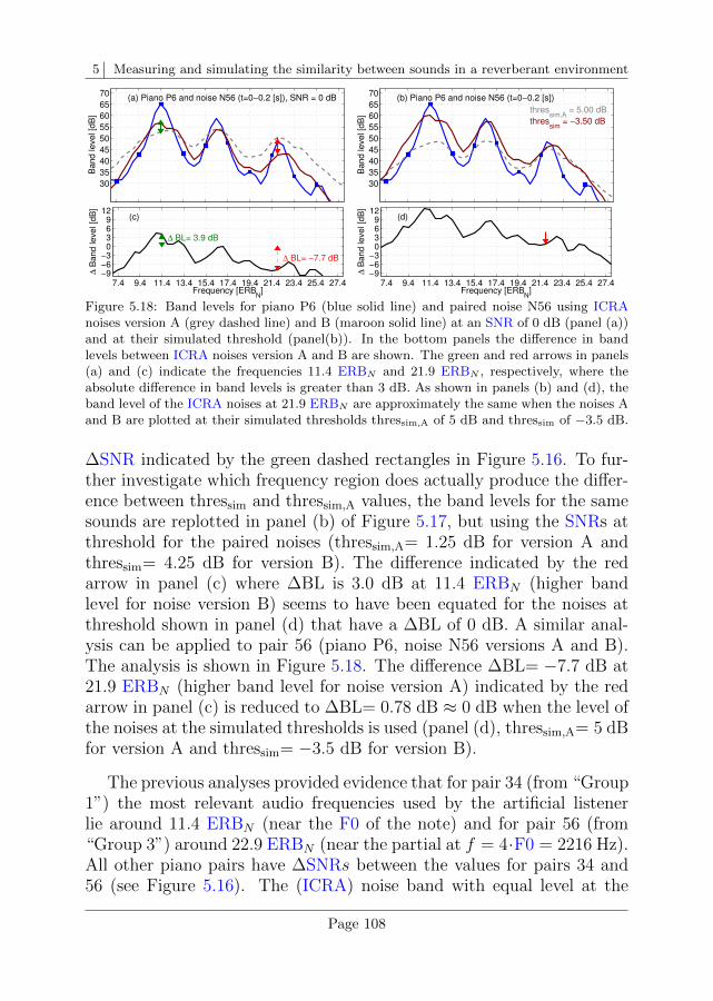
5 Measuring and simulating the similarity between sounds in a reverberant environment
7.4 9.4 11.4 13.4 15.4 17.4 19.4 21.4 23.4 25.4 27.4
30
35
40
45
50
55
60
65
70
Frequency [ERBN
]
Band level [d
B]
P5
7.4 9.4 11.4 13.4 15.4 17.4 19.4 21.4 23.4 25.4 27.4
30
35
40
45
50
55
60
65
70
Frequency [ERBN
]
Band le
vel [d
B]
(a) Piano P6 and noise N56 (t=0−0.2 [s]), SNR = 0 dB
7.4 9.4 11.4 13.4 15.4 17.4 19.4 21.4 23.4 25.4 27.4
30
35
40
45
50
55
60
65
70
Frequency [ERBN
]
Band level [d
B]
P5
7.4 9.4 11.4 13.4 15.4 17.4 19.4 21.4 23.4 25.4 27.4
30
35
40
45
50
55
60
65
70
Frequency [ERBN
]
Band le
vel [d
B]
thressim
= −3.50 dB
thressim,A
= 5.00 dB
(b) Piano P6 and noise N56 (t=0−0.2 [s])
7.4 9.4 11.4 13.4 15.4 17.4 19.4 21.4 23.4 25.4 27.4−9−6−3
0369
12
∆ B
and level [d
B]
Frequency [ERBN
]
∆ BL= −7.7 dB
∆ BL= 3.9 dB
(c)
7.4 9.4 11.4 13.4 15.4 17.4 19.4 21.4 23.4 25.4 27.4−9−6−3
0369
12
∆ B
and level [d
B]
Frequency [ERBN
]
(d)
Figure 5.18: Band levels for piano P6 (blue solid line) and paired noise N56 using ICRAnoises version A (grey dashed line) and B (maroon solid line) at an SNR of 0 dB (panel (a))and at their simulated threshold (panel(b)). In the bottom panels the difference in bandlevels between ICRA noises version A and B are shown. The green and red arrows in panels(a) and (c) indicate the frequencies 11.4 ERBN and 21.9 ERBN , respectively, where theabsolute difference in band levels is greater than 3 dB. As shown in panels (b) and (d), theband level of the ICRA noises at 21.9 ERBN are approximately the same when the noises Aand B are plotted at their simulated thresholds thressim,A of 5 dB and thressim of −3.5 dB.
∆SNR indicated by the green dashed rectangles in Figure 5.16. To fur-ther investigate which frequency region does actually produce the differ-ence between thressim and thressim,A values, the band levels for the samesounds are replotted in panel (b) of Figure 5.17, but using the SNRs atthreshold for the paired noises (thressim,A= 1.25 dB for version A andthressim= 4.25 dB for version B). The difference indicated by the redarrow in panel (c) where ∆BL is 3.0 dB at 11.4 ERBN (higher bandlevel for noise version B) seems to have been equated for the noises atthreshold shown in panel (d) that have a ∆BL of 0 dB. A similar anal-ysis can be applied to pair 56 (piano P6, noise N56 versions A and B).The analysis is shown in Figure 5.18. The difference ∆BL= −7.7 dB at21.9 ERBN (higher band level for noise version A) indicated by the redarrow in panel (c) is reduced to ∆BL= 0.78 dB ≈ 0 dB when the level ofthe noises at the simulated thresholds is used (panel (d), thressim,A= 5 dBfor version A and thressim= −3.5 dB for version B).
The previous analyses provided evidence that for pair 34 (from “Group1”) the most relevant audio frequencies used by the artificial listenerlie around 11.4 ERBN (near the F0 of the note) and for pair 56 (from“Group 3”) around 22.9 ERBN (near the partial at f = 4·F0 = 2216 Hz).All other piano pairs have ∆SNRs between the values for pairs 34 and56 (see Figure 5.16). The (ICRA) noise band with equal level at the
Page 108
5 Measuring and simulating the similarity between sounds in a reverberant environment
Ch
ap
ter
5
corresponding thresholds thressim,A and thressim will therefore be in thespectral range between harmonics F0 and 4·F0 of the C#5 note.
If the efficiency of the two noises is to be evaluated in terms of theamount of noise needed to mask the properties of the piano sounds, thenICRA noises version A perform “better” because for the same overall(broad-band) noise level the discrimination thresholds have on averagehigher SNRs (lower noise level) compared to ICRA noises version B:∆SNR = −3.25 dB (IQR between −4.25 and −0.75 dB). This “betterperformance” is, however, at the expense of a gradual level mismatchtowards higher frequencies of the noises with respect to the sounds to bemasked. If the efficiency of the noises is to be evaluated in terms of howwell do the spectro-temporal properties of the noise follow the propertiesof the sounds to be masked then ICRA noises version B perform better.
5.5 Conclusion
In this chapter the instrument-in-noise method of Chapters 3 and 4 hasbeen applied to the same dataset of pianos to which the effect of re-verberation was added by digital convolution. Experimental thresholdsthresexp were collected using a new version of the ICRA noise algorithmand compared with Euclidean distances obtained from experimental tri-adic comparisons dij exp. The results of both methods had a similarcorrelation compared to the values reported in Chapter 3, with a Pear-son correlation rp(18) = −0.49, p = 0.03 and a Spearman correlationrs(19) = −0.65, p = 0.001. Using the same simulation scheme as inChapter 4, estimates thressim of the instrument-in-noise method were ob-tained using the PEMO model. In order to bring the thressim thresholdsto the range of thresexp, the observation period of the artificial listenerhad to be reduced to tobs = 0.20 s. The obtained thressim values hadcorrelations of rp(18) = 0.58, p < 0.01, and rs(19) = 0.61, p < 0.001.
An information-based analysis of the internal representations obtainedfrom the PEMO model showed that the effect of a 3-s long reverberationon our set of piano notes (C#5) increased the importance of the au-dio frequency bands (Im/Itot) comprising the first five harmonics abovethe F0 (between 15.4 and 25.4 ERBN) and decreased the importanceof the band centred at the F0 of the note with respect to the weight-ings found for the anechoic pianos in Chapter 4. In terms of the in-formation conveyed by the modulation filters (Ik/Itot), the filters 6 − 9(mfc = 46.3−128.6 Hz) increased their relative weighting while the lower
Page 109
5 Measuring and simulating the similarity between sounds in a reverberant environment
modulation filters (mfc ≤ 10 Hz) decreased their importance.
Further simulations were used to address the following aspects: (1) theestimation of discrimination thresholds thressim,A using ICRA noises ver-sion A, and (2) the simulation of the triadic comparison task. The es-timated thressim,A and thressim values had correlations rp(18) = 0.61,p < 0.01, and rs(19) = 0.56, p < 0.001. For the first aspect, an analysisbased on the difference between thresholds indicated that the decisionsof the artificial listener are importantly influenced by the informationcontained in the spectral region between F0 and 4 · F0. For the secondaspect, we had a limited success with the simulation of the triadic com-parisons, where the simulated distances dij sim had only medium to lowcorrelations with both experimental and simulated thresholds. An anal-ysis of the resulting MDS spaces revealed that only their first and thirddimensions were correlated with high or moderate values rp(5) = 0.96and r(5) = 0.54, respectively. It is important to note, however, thatthe same simulation approach reached only a moderate correlation withdij exp in Chapter 3. Moreover we found some evidence for an increase inthe task difficulty with respect to the experiments using anechoic pianos(Chapter 3). In the instrument-in-noise method, for instance, the con-sistency in the staircases adopting the exclusion criterion of Chapter 3would have led to more exclusions: 38 staircases (18.1% of the data) incontrast to the 24 staircases (11.4%) excluded using a more permissiblecriterion. Additionally, the goodness of fit of the MDS space (from theexperimental sessions) had a somewhat poorer fit with respect to the col-lected similarity matrix. This may be due to a more variable weightingof psychological dimensions for different participants.
In summary, the experimental results presented in this chapter showedthat instrument-in-noise thresholds are similarly correlated with Eu-clidean distances from the triadic comparisons for the perceptual simi-larity assessment of reverberant piano sounds with respect to the resultsreported in Chapter 3 for anechoic sounds. Furthermore, simulations ofthe instrument-in-noise thresholds using the PEMO model had a simi-lar degree of success with respect to the simulations of Chapter 4. Wecan conclude that the results of this chapter further support the valid-ity of the auditory modelling approach of Chapter 4 when the effect ofreverberation is applied to the dataset of sounds.
Page 110
6 Simulating the perceived reverberation indifferent room acoustic environments using abinaural auditory model1
In this chapter an alternative way to use the unified modelling frame-work introduced in Chapter 4 is presented. Particularly, a binauralmodel is used to compute estimates of perceived reverberation –knownas reverberance– for a set of musical instrument sounds that are au-ralised using eight different acoustic environments. The binaural modelprocesses left and right-ear channels in a similar manner as the auditoryPEMO model used in the previous chapters, but the central processorconverts the (left- and right-ear) internal representations into a metricof reverberance PREV. This central processor is based on the idea ofstream segregation, adopted from the field of auditory scene analysis,rather than on the optimal detector used in previous chapters to ap-proach the problem of perceptual similarity among sounds.
In the first part of the chapter, PREV estimates obtained from thebinaural auditory model, originally described and validated by van Dorp(2011) and van Dorp, de Vries, and Lindau (2013), are compared withthe room acoustic parameters of reverberation time (T30) and early decaytime (EDT). For this comparison, 90-s music excerpts of an orchestraconsisting of 23 instrument sections are used. The simulation resultsshow that although PREV has a higher correlation with EDT than withT30, this relationship depends on the properties of the instruments. Fur-ther analyses show that PREV depends on the presentation level andthat for instruments with similar critical-band spectrum, PREV followsa similar trend across acoustic conditions.
In order to obtain experimental evidence of the dependency of rever-berance on the properties of the sounds being tested, a listening test
1This chapter is partly based on: A. Osses, A. Kohlrausch, W. Lachenmayr, and E. Mommertz(2017). Predicting the perceived reverberation in different room acoustic environments using abinaural model. J. Acoust. Soc. Am., 141(4), EL381-EL387. http://doi.org/10.1121/1.4979853
Page 111
6 Simulating the perceived reverberation using a binaural model
is presented in the second part of this chapter. The stimuli used inthe listening test correspond to a subset of 8 musical instrument soundsthat had been used in the initial simulations. The experimental resultssupport the hypothesis that the sensation of reverberance is instrument-dependent. Furthermore, these results are used to evaluate the validityof the PREV estimates obtained from the binaural model.
6.1 Introduction
A set of binaural room impulse responses (BRIRs) is usually measured inorder to evaluate the acoustic characteristics of a room. Out of these im-pulse responses conventional descriptors such as reverberation time (RT)or, in this chapter, T30, EDT and clarity index (C80) are obtained. Toobtain those parameters, the guidelines established in the internationalstandard ISO 3382-1 (ISO, 2009) can be followed. This guarantees areproducibility of the measurement results. The measurements are oftenperformed in empty rooms. Since the acoustic descriptors do differ whenmeasured in empty or occupied halls (see, e.g., Beranek, 2004) the lat-ter condition is always of interest, especially in the context of a concerthall or an opera house. Partly motivated by this idea, van Dorp et al.(2013) suggested the use of a time-domain binaural auditory model toestimate room acoustic parameters. Their rationale was that sound sam-ples recorded or simulated in a given acoustic environment convey roomacoustic cues that can be extracted by a binaural auditory model. A sim-ilar assumption was made by Klockgether and van de Par (2014, 2016)who used excerpts of violin, guitar, and snare drum sounds to investi-gate the spatial attributes of listener envelopment (LEV) and apparentsource width (ASW), and the JND in the binaural cues of interaural leveldifference (ILD) and interaural time difference (ITD) in three acousticenvironments.
During the development of their binaural model, van Dorp et al.(2013) conducted four listening experiments using two sounds (speechand cello), which were auralised using 27 BRIRs. They found that theirmodel estimates were highly correlated with the subjective percept ofreverberation, known as reverberance.
Motivated by the success of their model, in this chapter we presentan extension of their work by analysing a more diverse set of sounds inacoustic conditions that are typical for rehearsal and music performancevenues. Our set of sounds consisted of 23 instruments from a 90-s ex-
Page 112
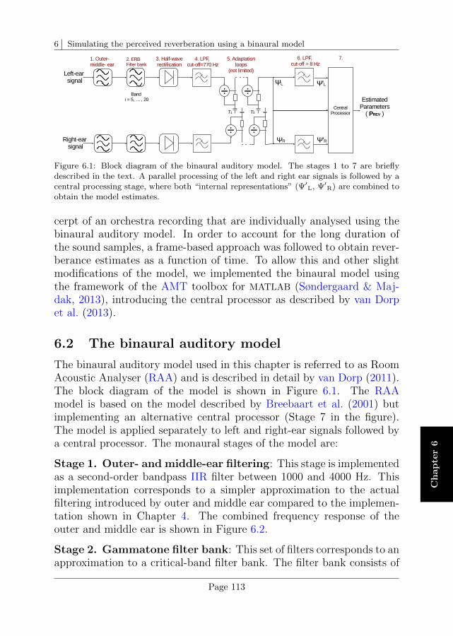
6 Simulating the perceived reverberation using a binaural model
Ch
ap
ter
6
Figure 6.1: Block diagram of the binaural auditory model. The stages 1 to 7 are brieflydescribed in the text. A parallel processing of the left and right ear signals is followed by acentral processing stage, where both “internal representations” (Ψ′L, Ψ′R) are combined toobtain the model estimates.
cerpt of an orchestra recording that are individually analysed using thebinaural auditory model. In order to account for the long duration ofthe sound samples, a frame-based approach was followed to obtain rever-berance estimates as a function of time. To allow this and other slightmodifications of the model, we implemented the binaural model usingthe framework of the AMT toolbox for MATLAB (Søndergaard & Maj-dak, 2013), introducing the central processor as described by van Dorpet al. (2013).
6.2 The binaural auditory model
The binaural auditory model used in this chapter is referred to as RoomAcoustic Analyser (RAA) and is described in detail by van Dorp (2011).The block diagram of the model is shown in Figure 6.1. The RAAmodel is based on the model described by Breebaart et al. (2001) butimplementing an alternative central processor (Stage 7 in the figure).The model is applied separately to left and right-ear signals followed bya central processor. The monaural stages of the model are:
Stage 1. Outer- and middle-ear filtering: This stage is implementedas a second-order bandpass IIR filter between 1000 and 4000 Hz. Thisimplementation corresponds to a simpler approximation to the actualfiltering introduced by outer and middle ear compared to the implemen-tation shown in Chapter 4. The combined frequency response of theouter and middle ear is shown in Figure 6.2.
Stage 2. Gammatone filter bank: This set of filters corresponds to anapproximation to a critical-band filter bank. The filter bank consists of
Page 113
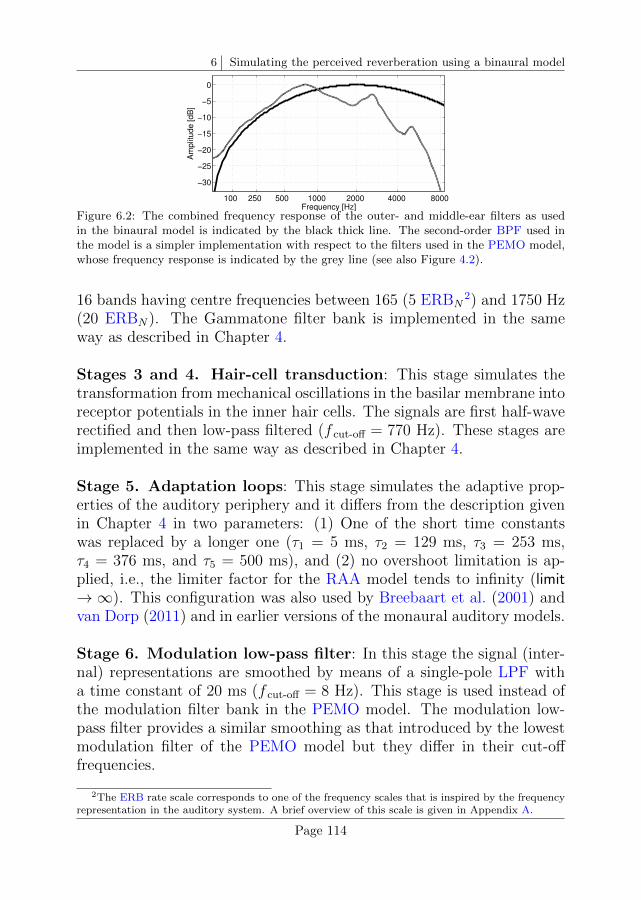
6 Simulating the perceived reverberation using a binaural model
100 250 500 1000 2000 4000 8000
−30
−25
−20
−15
−10
−5
0
Frequency [Hz]
Am
plit
ud
e [
dB
]
Figure 6.2: The combined frequency response of the outer- and middle-ear filters as usedin the binaural model is indicated by the black thick line. The second-order BPF used inthe model is a simpler implementation with respect to the filters used in the PEMO model,whose frequency response is indicated by the grey line (see also Figure 4.2).
16 bands having centre frequencies between 165 (5 ERBN2) and 1750 Hz
(20 ERBN). The Gammatone filter bank is implemented in the sameway as described in Chapter 4.
Stages 3 and 4. Hair-cell transduction: This stage simulates thetransformation from mechanical oscillations in the basilar membrane intoreceptor potentials in the inner hair cells. The signals are first half-waverectified and then low-pass filtered (f cut-off = 770 Hz). These stages areimplemented in the same way as described in Chapter 4.
Stage 5. Adaptation loops: This stage simulates the adaptive prop-erties of the auditory periphery and it differs from the description givenin Chapter 4 in two parameters: (1) One of the short time constantswas replaced by a longer one (τ1 = 5 ms, τ2 = 129 ms, τ3 = 253 ms,τ4 = 376 ms, and τ5 = 500 ms), and (2) no overshoot limitation is ap-plied, i.e., the limiter factor for the RAA model tends to infinity (limit→∞). This configuration was also used by Breebaart et al. (2001) andvan Dorp (2011) and in earlier versions of the monaural auditory models.
Stage 6. Modulation low-pass filter: In this stage the signal (inter-nal) representations are smoothed by means of a single-pole LPF witha time constant of 20 ms (f cut-off = 8 Hz). This stage is used instead ofthe modulation filter bank in the PEMO model. The modulation low-pass filter provides a similar smoothing as that introduced by the lowestmodulation filter of the PEMO model but they differ in their cut-offfrequencies.
2The ERB rate scale corresponds to one of the frequency scales that is inspired by the frequencyrepresentation in the auditory system. A brief overview of this scale is given in Appendix A.
Page 114
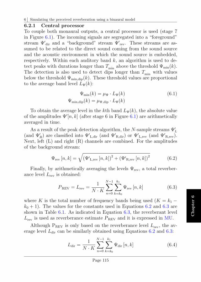
6 Simulating the perceived reverberation using a binaural model
Ch
ap
ter
6
6.2.1 Central processorTo couple both monaural outputs, a central processor is used (stage 7in Figure 6.1). The incoming signals are segregated into a “foreground”stream Ψ′dir and a “background” stream Ψ′rev. These streams are as-sumed to be related to the direct sound coming from the sound sourceand the acoustic environment in which the sound source is embedded,respectively. Within each auditory band k, an algorithm is used to de-tect peaks with durations longer than Tmin above the threshold Ψmin(k).The detection is also used to detect dips longer than Tmin with valuesbelow the threshold Ψmin,dip(k). These threshold values are proportionalto the average band level LΨ(k):
Ψmin(k) = µΨ · LΨ(k) (6.1)
Ψmin,dip(k) = µΨ,dip · LΨ(k)
To obtain the average level in the kth band LΨ(k), the absolute valueof the amplitudes Ψ′[n, k] (after stage 6 in Figure 6.1) are arithmeticallyaveraged in time.
As a result of the peak detection algorithm, the N -sample streams Ψ′L(and Ψ′R) are classified into Ψ′L,dir (and Ψ′R,dir) or Ψ′L,rev (and Ψ′R,rev).Next, left (L) and right (R) channels are combined. For the amplitudesof the background stream:
Ψrev [n, k] =
√(Ψ′L,rev [n, k])2 + (Ψ′R,rev [n, k])2 (6.2)
Finally, by arithmetically averaging the levels Ψrev, a total reverber-ance level Lrev is obtained:
PREV = Lrev =1
N ·K
N−1∑n=0
k1∑k=k0
Ψrev [n, k] (6.3)
where K is the total number of frequency bands being used (K = k1 −k0 + 1). The values for the constants used in Equations 6.2 and 6.3 areshown in Table 6.1. As indicated in Equation 6.3, the reverberant levelLrev is used as reverberance estimate PREV and it is expressed in MU.
Although PREV is only based on the reverberance level Lrev , the av-erage level Ldir can be similarly obtained using Equations 6.2 and 6.3:
Ldir =1
N ·K
N−1∑n=0
k1∑k=k0
Ψdir [n, k] (6.4)
Page 115

6 Simulating the perceived reverberation using a binaural model
Table 6.1: Parameters of the RAA model as reported by van Dorp (“Original”) and as usedin our implementation (“Our”) for estimating PREV.
Parameter Values: Our (Original) Descriptionk0 − k1 5-20 (5-20) Initial and final spectral band number (ERBN ) used in
the estimation (K = 16 bands)fc [Hz] 174-1807 (168-1836) Centre frequencies of the initial and final ERB band used
in the estimationµΨ 0.34 (7.49 · 10−3) Constant factor for peak detection
µΨ,dip −0.06 (−1.33 · 10−3) Constant factor for dip detection|µΨ/µΨ,dip| 5.63 (5.63) Ratio between peak detection factorsTmin [ms] 63.1 (63.1) Minimum peak/dip duration for the foreground stream
The level Ldir is used by the central processor of the model to obtainthree other room acoustics estimates which are not described in thisthesis (van Dorp, 2011; van Dorp et al., 2013).
6.2.2 Differences in the current implementation
Our implementation of the binaural model differs slightly from the orig-inal RAA model. We did not account for the absolute threshold of hear-ing, originally implemented as a frequency-dependent scaling before andafter stage 5 (adaptation loops). As a consequence of this, the amplitudesof the internal representations differ (leading to different band levels LΨ)and, therefore, different µ-factors were required to get an appropriatesegregation of the foreground and background streams. The parametersused in our implementation are shown in Table 6.1. In order to dealwith sounds containing silent sections, only those segments where eachinstrument was active were considered.
6.3 Study case: Reverberance of differentorchestra instruments
6.3.1 Rooms
Four rooms have been simulated in the software Odeon Auditorium v.13using the suggested accuracy “engineering”. Three of the rooms weresimulated with different absorptions, producing a total number of 8acoustic environments (i.e., 8 “rooms”). Some information about the8 acoustic environments is given in Table 6.2. The acoustic parameterswere estimated at the location of a binaural listener arbitrarily placed7 m in front of the stage in all cases. The room A is a medium-sizedmusic venue with a coupled ceiling space, simulated without (A) andwith absorption on the walls and the ceiling (Aabs). The room B is alarge-sized concert hall, simulated without (B) and with all interior walls
Page 116
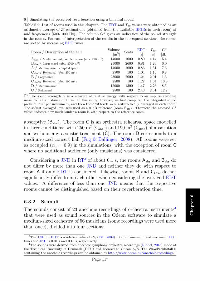
6 Simulating the perceived reverberation using a binaural model
Ch
ap
ter
6
Table 6.2: List of rooms used in this chapter. The EDT and T30 values were obtained as anarithmetic average of 23 estimations (obtained from the available BRIRs in each room) atmid frequencies (500-1000 Hz). The column G* gives an indication of the sound strengthin the rooms. For ease of interpretation of the results in the subsequent sections, the roomsare sorted by increasing EDT times.
Room / Description of the hallVolume
SeatsEDT T30 G*
[m3] [s] [s] [dB]Aabs / Medium-sized, coupled space (abs. 720 m2) 14000 1000 0.80 1.14 5.4Babs / Large-sized (abs. 3700 m2) 23000 2600 0.81 1.20 0.0A / Medium-sized, coupled space 14000 1000 0.83 1.51 7.3Cabs1/ Rehearsal (abs. 250 m2) 2500 100 1.04 1.16 9.8B / Large-sized 23000 2600 1.24 2.01 1.3Cabs2/ Rehearsal (abs. 190 m2) 2500 100 1.27 1.34 10.8D / Medium-sized 15000 1300 1.47 2.23 8.5C / Rehearsal 2500 100 2.48 2.51 12.7
(*) The sound strength G is a measure of relative energy with respect to an impulse responsemeasured at a distance of 10 m. In this study, however, we first computed the integrated soundpressure level per instrument, and then those 23 levels were arithmetically averaged in each room.The softest averaged level was used as a 0 dB reference (room Babs). Therefore the assessed G*values indicate how much louder a room is with respect to the reference room.
absorptive (Babs). The room C is an orchestra rehearsal space modelledin three conditions: with 250 m2 (Cabs1) and 190 m2 (Cabs2) of absorptionand without any acoustic treatment (C). The room D corresponds to amedium-sized concert hall (Fog & Ballinger, 2008). All rooms were setas occupied (αω = 0.9) in the simulations, with the exception of room Cwhere no additional audience (only musicians) was considered.
Considering a JND in RT3 of about 0.1 s, the rooms Aabs and Babs donot differ by more than one JND and neither they do with respect toroom A if only EDT is considered. Likewise, rooms B and Cabs2 do notsignificantly differ from each other when considering the averaged EDTvalues. A difference of less than one JND means that the respectiverooms cannot be distinguished based on their reverberation time.
6.3.2 Stimuli
The sounds consist of 23 anechoic recordings of orchestra instruments4
that were used as sound sources in the Odeon software to simulate amedium-sized orchestra of 56 musicians (some recordings were used morethan once), divided into four sections:
3The JND for EDT is a relative value of 5% (ISO, 2009). For our minimum and maximum EDTtimes the JND is 0.04 s and 0.13 s, respectively.
4The sounds were derived from anechoic symphony orchestra recordings (Rindel, 2015) made atthe Technical University of Denmark (DTU) and licensed to Odeon A/S. The WavePackInstall IIcontaining the anechoic recordings can be obtained at http://www.odeon.dk/anechoic-recordings.
Page 117
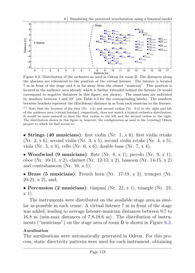
6 Simulating the perceived reverberation using a binaural model
0 1 2 3 4 5 6 7 8 9 10 11 12 13 14 15 16 17
−8
−6
−4
−2
0
2
4
6
8
1(8.4) 2(9.4)
2(9.2) 1(10.1)
1(9.6) 2(10.5)
2(10.6) 1(11.4)
1(11.2) 2(11.9)
2(12.1) 1(12.9)
3(8.0) 4(9.0)
4(8.6) 3(9.6)
3(8.9) 4(9.8)
4(9.7) 3(10.6)
3(10.1) 4(11.0)
5(10.0) 5(11.0)
5(10.5) 5(11.5)
5(10.7) 5(11.7)
5(11.4) 5(12.4)
6(10.2) 6(11.2)
6(11.1) 6(12.0)
6(12.1) 6(13.0)
7(14.8)
7(14.8)
7(14.9)
7(15.0)
9(13.3)
8(13.1)
10 (13.0)
11 (13.0)
13 (14.7)
12 (14.6)
14 (14.5)
15 (14.5)
16 (14.6)
17 (14.3)
18 (14.1)
19 (13.9)
20 (16.0)
21 (16.1)
22 (16.0)
23 (16.2)
listener
Aarhus, distance to listener [m] between brackets
Distance [m]
Dis
tan
ce
[m
]Stage
Figure 6.3: Distribution of the orchestra as used in Odeon for room D. The distances alongthe abscissa are referenced to the position of the virtual listener. The listener is located7 m in front of the stage and 8 m far away from the closest “musician”. This position islocated in the audience area already which is further extended behind the listener (it wouldcorrespond to negative distances in this figure, not shown). The musicians are indicatedby numbers between 1 and 23∗ (see Table 6.3 for the corresponding labels). The numbersbetween brackets represent the (Euclidean) distance in m from each musician to the listener.(*) Note that the location of the first (Nr. 1-2) and second violins (Nr. 3-4) to the right and leftof the audience area (virtual listener), respectively, does not match a typical orchestra distribution.It would be more natural to have the first violins to the left and the second violins to the right.The distribution shown in this figure is, however, the configuration as used in the (existing) Odeonproject to which we had access to.
• Strings (40 musicians): first violin (Nr. 1, x 6), first violin retake(Nr. 2, x 6), second violin (Nr. 3, x 5), second violin retake (Nr. 4, x 5),viola (Nr. 5, x 8), cello (Nr. 6, x 6), double bass (Nr. 7, x 4);
• Woodwind (9 musicians): flute (Nr. 8, x 1), piccolo (Nr. 9, x 1),oboe (Nr. 10-11, x 2), clarinet (Nr. 12-13, x 2), bassoon (Nr. 14-15, x 2)and contrabassoon (Nr. 16, x 1);
• Brass (5 musicians): French horn (Nr. 17-19, x 3), trumpet (Nr.20-21, x 2), and;
• Percussion (2 musicians): timpani (Nr. 22, x 1), triangle (Nr. 23,x 1).
The instruments were distributed on the available stage area as simi-lar as possible in each venue. A virtual listener 7 m in front of the stagewas added, leading to average listener-musician distances between 9.7 to16.8 m (min-max distances of 7.8-18.6 m). The distribution of instru-ments (“musicians”) on the stage area of room D is shown in Figure 6.3.
Auralisation
The auralisations were automatically generated in Odeon. For this pro-cess, static directivity patterns were used for each instrument, obtaining
Page 118
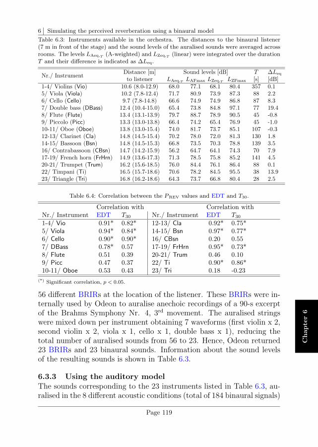
6 Simulating the perceived reverberation using a binaural model
Ch
ap
ter
6
Table 6.3: Instruments available in the orchestra. The distances to the binaural listener(7 m in front of the stage) and the sound levels of the auralised sounds were averaged acrossrooms. The levels LAeq,T (A-weighted) and LZeq,T (linear) were integrated over the durationT and their difference is indicated as ∆Leq.
Nr./ InstrumentDistance [m] Sound levels [dB] T ∆Leq
to listener LAeq,T LAFmax LZeq,T LZFmax [s] [dB]1-4/ Violins (Vio) 10.6 (8.0-12.9) 68.0 77.1 68.1 80.4 357 0.15/ Viola (Viola) 10.2 (7.8-12.4) 71.7 80.9 73.9 87.3 88 2.26/ Cello (Cello) 9.7 (7.8-14.8) 66.6 74.9 74.9 86.8 87 8.37/ Double bass (DBass) 12.4 (10.4-15.0) 65.4 73.8 84.8 97.1 77 19.48/ Flute (Flute) 13.4 (13.1-13.9) 79.7 88.7 78.9 90.5 45 -0.89/ Piccolo (Picc) 13.3 (13.0-13.8) 66.4 74.2 65.4 76.9 45 -1.010-11/ Oboe (Oboe) 13.8 (13.0-15.4) 74.0 81.7 73.7 85.1 107 -0.312-13/ Clarinet (Cla) 14.8 (14.5-15.4) 70.2 78.0 72.0 81.3 130 1.814-15/ Bassoon (Bsn) 14.8 (14.5-15.3) 66.8 73.5 70.3 78.8 139 3.516/ Contrabassoon (CBsn) 14.7 (14.2-15.9) 56.2 64.7 64.1 74.3 70 7.917-19/ French horn (FrHrn) 14.9 (13.6-17.3) 71.3 78.5 75.8 85.2 141 4.520-21/ Trumpet (Trum) 16.2 (15.6-18.5) 76.0 84.4 76.1 86.4 88 0.122/ Timpani (Ti) 16.5 (15.7-18.6) 70.6 78.2 84.5 95.5 38 13.923/ Triangle (Tri) 16.8 (16.2-18.6) 64.3 73.7 66.8 80.4 28 2.5
Table 6.4: Correlation between the PREV values and EDT and T30.
Correlation with Correlation withNr./ Instrument EDT T30 Nr./ Instrument EDT T30
1-4/ Vio 0.91* 0.82* 12-13/ Cla 0.92* 0.75*5/ Viola 0.94* 0.84* 14-15/ Bsn 0.97* 0.77*6/ Cello 0.90* 0.90* 16/ CBsn 0.20 0.557/ DBass 0.78* 0.57 17-19/ FrHrn 0.95* 0.73*8/ Flute 0.51 0.39 20-21/ Trum 0.46 0.109/ Picc 0.47 0.37 22/ Ti 0.90* 0.86*10-11/ Oboe 0.53 0.43 23/ Tri 0.18 -0.23
(*) Significant correlation, p < 0.05.
56 different BRIRs at the location of the listener. These BRIRs were in-ternally used by Odeon to auralise anechoic recordings of a 90-s excerptof the Brahms Symphony Nr. 4, 3rd movement. The auralised stringswere mixed down per instrument obtaining 7 waveforms (first violin x 2,second violin x 2, viola x 1, cello x 1, double bass x 1), reducing thetotal number of auralised sounds from 56 to 23. Hence, Odeon returned23 BRIRs and 23 binaural sounds. Information about the sound levelsof the resulting sounds is shown in Table 6.3.
6.3.3 Using the auditory modelThe sounds corresponding to the 23 instruments listed in Table 6.3, au-ralised in the 8 different acoustic conditions (total of 184 binaural signals)
Page 119
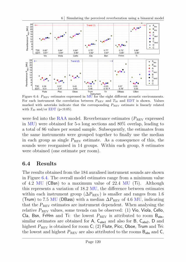
6 Simulating the perceived reverberation using a binaural model
Vio Viola Cello Cla Bsn FrHrn Ti
468
1012141618202224
T30: EDT:
Re
ve
rbe
ran
ce
PR
EV [
MU
]
Instrument
0.82* 0.91*
0.84* 0.94*
0.90* 0.90*
0.75* 0.92*
0.77* 0.97*
0.73* 0.95*
0.86* 0.90*
Trend (1) →← Aabs
Babs
A
Cabs1
B
Cabs2
D
C
Flute Picc Oboe Trum Tri DBass CBsn
468
1012141618202224
T30: EDT:
Re
ve
rbe
ran
ce
PR
EV [
MU
]
Instrument
0.39 0.51
0.37 0.47
0.43 0.53
0.10 0.46
−0.23 0.18
0.57 0.78*
0.55 0.20
Trend (2) →← Aabs
Babs
A
Cabs1
B
Cabs2
D
C
Figure 6.4: PREV estimates expressed in MU for the eight different acoustic environments.For each instrument the correlation between PREV and T30 and EDT is shown. Valuesmarked with asterisks indicate that the corresponding PREV estimate is linearly relatedwith T30 and/or EDT (p<0.05).
were fed into the RAA model. Reverberance estimates (PREV expressedin MU) were obtained for 5-s long sections and 80% overlap, leading toa total of 86 values per sound sample. Subsequently, the estimates fromthe same instruments were grouped together to finally use the medianin each group as single PREV estimate. As a consequence of this, thesounds were reorganised in 14 groups. Within each group, 8 estimateswere obtained (one estimate per room).
6.4 Results
The results obtained from the 184 auralised instrument sounds are shownin Figure 6.4. The overall model estimates range from a minimum valueof 4.2 MU (CBsn) to a maximum value of 22.4 MU (Ti). Althoughthis represents a variation of 18.2 MU, the difference between estimateswithin each instrument group (∆PREV) is smaller and ranges from 1.6(Trum) to 7.5 MU (DBass) with a median ∆PREV of 4.6 MU, indicatingthat the PREV estimates are instrument dependent. When analysing therelative PREV values, some trends can be observed: (1) Vio, Viola, Cello,Cla, Bsn, FrHrn and Ti: the lowest PREV is attributed to room Babs,similar estimates are obtained for A, Cabs1 and also for B, Cabs2, D andhighest PREV is obtained for room C; (2) Flute, Picc, Oboe, Trum and Tri:the lowest and highest PREV are also attributed to the rooms Babs and C,
Page 120
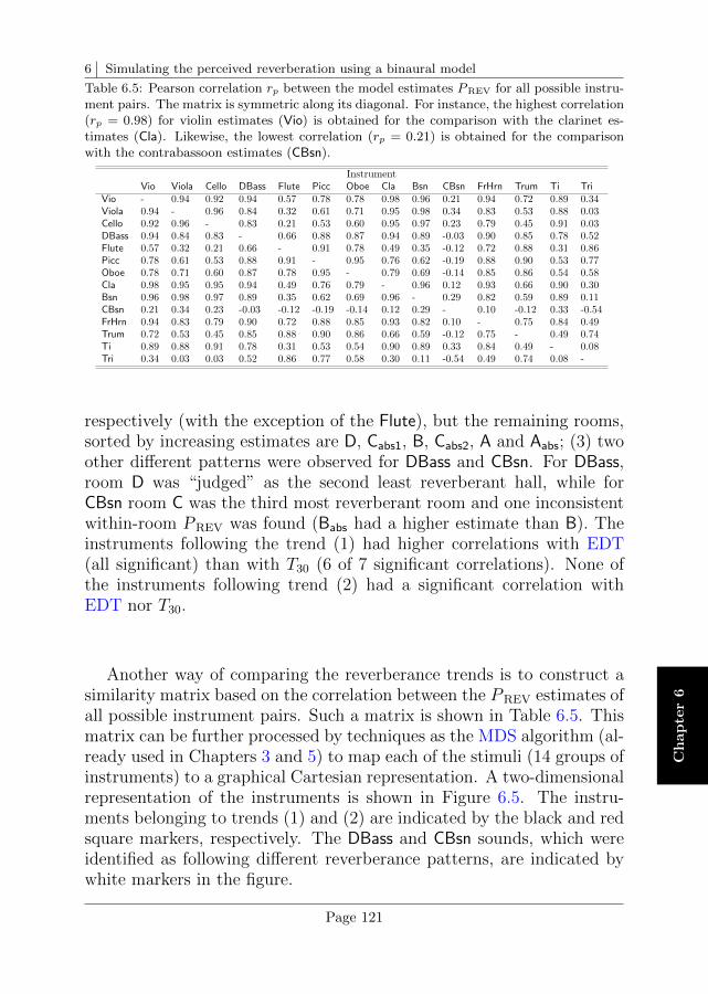
6 Simulating the perceived reverberation using a binaural model
Ch
ap
ter
6
Table 6.5: Pearson correlation rp between the model estimates PREV for all possible instru-ment pairs. The matrix is symmetric along its diagonal. For instance, the highest correlation(rp = 0.98) for violin estimates (Vio) is obtained for the comparison with the clarinet es-timates (Cla). Likewise, the lowest correlation (rp = 0.21) is obtained for the comparisonwith the contrabassoon estimates (CBsn).
InstrumentVio Viola Cello DBass Flute Picc Oboe Cla Bsn CBsn FrHrn Trum Ti Tri
Vio - 0.94 0.92 0.94 0.57 0.78 0.78 0.98 0.96 0.21 0.94 0.72 0.89 0.34Viola 0.94 - 0.96 0.84 0.32 0.61 0.71 0.95 0.98 0.34 0.83 0.53 0.88 0.03Cello 0.92 0.96 - 0.83 0.21 0.53 0.60 0.95 0.97 0.23 0.79 0.45 0.91 0.03DBass 0.94 0.84 0.83 - 0.66 0.88 0.87 0.94 0.89 -0.03 0.90 0.85 0.78 0.52Flute 0.57 0.32 0.21 0.66 - 0.91 0.78 0.49 0.35 -0.12 0.72 0.88 0.31 0.86Picc 0.78 0.61 0.53 0.88 0.91 - 0.95 0.76 0.62 -0.19 0.88 0.90 0.53 0.77Oboe 0.78 0.71 0.60 0.87 0.78 0.95 - 0.79 0.69 -0.14 0.85 0.86 0.54 0.58Cla 0.98 0.95 0.95 0.94 0.49 0.76 0.79 - 0.96 0.12 0.93 0.66 0.90 0.30Bsn 0.96 0.98 0.97 0.89 0.35 0.62 0.69 0.96 - 0.29 0.82 0.59 0.89 0.11CBsn 0.21 0.34 0.23 -0.03 -0.12 -0.19 -0.14 0.12 0.29 - 0.10 -0.12 0.33 -0.54FrHrn 0.94 0.83 0.79 0.90 0.72 0.88 0.85 0.93 0.82 0.10 - 0.75 0.84 0.49Trum 0.72 0.53 0.45 0.85 0.88 0.90 0.86 0.66 0.59 -0.12 0.75 - 0.49 0.74Ti 0.89 0.88 0.91 0.78 0.31 0.53 0.54 0.90 0.89 0.33 0.84 0.49 - 0.08Tri 0.34 0.03 0.03 0.52 0.86 0.77 0.58 0.30 0.11 -0.54 0.49 0.74 0.08 -
respectively (with the exception of the Flute), but the remaining rooms,sorted by increasing estimates are D, Cabs1, B, Cabs2, A and Aabs; (3) twoother different patterns were observed for DBass and CBsn. For DBass,room D was “judged” as the second least reverberant hall, while forCBsn room C was the third most reverberant room and one inconsistentwithin-room PREV was found (Babs had a higher estimate than B). Theinstruments following the trend (1) had higher correlations with EDT(all significant) than with T30 (6 of 7 significant correlations). None ofthe instruments following trend (2) had a significant correlation withEDT nor T30.
Another way of comparing the reverberance trends is to construct asimilarity matrix based on the correlation between the PREV estimates ofall possible instrument pairs. Such a matrix is shown in Table 6.5. Thismatrix can be further processed by techniques as the MDS algorithm (al-ready used in Chapters 3 and 5) to map each of the stimuli (14 groups ofinstruments) to a graphical Cartesian representation. A two-dimensionalrepresentation of the instruments is shown in Figure 6.5. The instru-ments belonging to trends (1) and (2) are indicated by the black and redsquare markers, respectively. The DBass and CBsn sounds, which wereidentified as following different reverberance patterns, are indicated bywhite markers in the figure.
Page 121
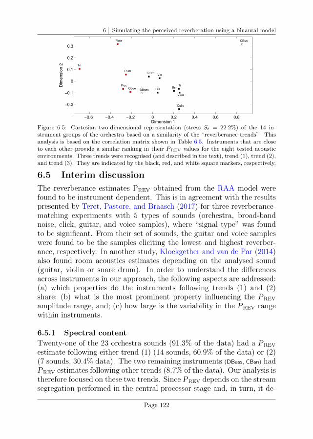
6 Simulating the perceived reverberation using a binaural model
−0.6 −0.4 −0.2 0 0.2 0.4 0.6 0.8
−0.2
−0.1
0
0.1
0.2
0.3
Vio
Viola
Cello
DBass
Flute
PiccOboe Cla
Bsn
CBsn
FrHrnTrum
Ti
Tri
Dimension 1
Dim
en
sio
n 2
Figure 6.5: Cartesian two-dimensional representation (stress St = 22.2%) of the 14 in-strument groups of the orchestra based on a similarity of the “reverberance trends”. Thisanalysis is based on the correlation matrix shown in Table 6.5. Instruments that are closeto each other provide a similar ranking in their PREV values for the eight tested acousticenvironments. Three trends were recognised (and described in the text), trend (1), trend (2),and trend (3). They are indicated by the black, red, and white square markers, respectively.
6.5 Interim discussion
The reverberance estimates PREV obtained from the RAA model werefound to be instrument dependent. This is in agreement with the resultspresented by Teret, Pastore, and Braasch (2017) for three reverberance-matching experiments with 5 types of sounds (orchestra, broad-bandnoise, click, guitar, and voice samples), where “signal type” was foundto be significant. From their set of sounds, the guitar and voice sampleswere found to be the samples eliciting the lowest and highest reverber-ance, respectively. In another study, Klockgether and van de Par (2014)also found room acoustics estimates depending on the analysed sound(guitar, violin or snare drum). In order to understand the differencesacross instruments in our approach, the following aspects are addressed:(a) which properties do the instruments following trends (1) and (2)share; (b) what is the most prominent property influencing the PREV
amplitude range, and; (c) how large is the variability in the PREV rangewithin instruments.
6.5.1 Spectral content
Twenty-one of the 23 orchestra sounds (91.3% of the data) had a PREV
estimate following either trend (1) (14 sounds, 60.9% of the data) or (2)(7 sounds, 30.4% data). The two remaining instruments (DBass, CBsn) hadPREV estimates following other trends (8.7% of the data). Our analysis istherefore focused on these two trends. Since PREV depends on the streamsegregation performed in the central processor stage and, in turn, it de-
Page 122
6 Simulating the perceived reverberation using a binaural model
Ch
ap
ter
6
pends on the average band level within each critical-band, the energy dis-tribution of two representative musical instruments following trends (1)and (2) is shown in panel (a) of Figure 6.6. The instruments followingtrend (1) had a balanced spectrum with contributions between roughly 5and 10% per band. The instruments following trend (2) had a monotonicincreasing contribution from nearly 0% (Picc) up to around 10% towardsthe upper bands. Therefore, in order to characterise a room obtainingone single estimate in the whole frequency range, it might be desirableto use instruments following trend (1). Since the auditory filters are nar-rower in the low frequency range a higher spectral level at low frequenciesis needed. An estimate that can give an indication of the frequency dis-tribution is the difference between linear and A-weighted levels. The in-struments following trend (1), with the exception of the violins, have a∆Leq that varies between 1.8 (Cla) and 13.9 dB (Ti) (see Table 6.3)5.
6.5.2 Frame-based valuesAs the individual instruments have dynamic changes along their 90 s ofmusic (6.7 ≤ LAFmax − LAeq,T ≤ 9.4 dB, see Table 6.3), we hypothesisedthat the reverberation estimate should also vary over time. The adoptedframe-based approach is useful to provide information about changes ofreverberance as a function of time. In Figure 6.6(b) the data points cor-responding to rooms Aabs and B are shown together with bars indicatingthe minimum and maximum PREV values over time. This variability issystematic in all instruments and the average range is ±3.2 MU.
6.5.3 Level dependencyTo investigate the dependency of PREV on presentation level, three of theinstrument groups (Vio, Flute, Ti) were plotted at two presentation lev-els with a level difference of 20 dB. The obtained estimates are shown inpanel (b) of Figure 6.6. For the three instrument groups, PREV increasedwhen increasing the presentation level. Evidence of the reverberance de-pendency on presentation level was given by Lee, Cabrera, and Martens(2012), where louder test samples required bigger adjustments to matchtheir reverberance with respect to a fixed-gain reference sample. Withinthe RAA model, the increase in the estimates seems to be further re-lated to the instrument spectral properties, with a stronger effect for theFlute (factor of 3) followed by the Ti (factor of 1.6) and the Violin (factorof 1.4).
5Although the level estimation shown in Table 6.3 is valid for the auralised sounds in room D,they are representative approximations of the level difference in the other seven acoustic conditions.
Page 123
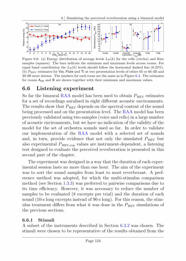
6 Simulating the perceived reverberation using a binaural model
5 6 7 8 9 10 11 12 13 14 15 16 17 18 19 200
2
4
6
8
10
12
ERBN
(Band Nr.)
Re
lative
en
erg
y [
%]
(a)
Vio/65 Vio/85 Flute/65 Flute/85 Ti/66 Ti/862
4
68
10
12
1416
18
20
22
24
Re
ve
rbe
ran
ce
PR
EV [
MU
]
Instrument / LZeq
[dB]
(b) Trend (1): Cello
Trend (2): Flute
Figure 6.6: (a) Energy distribution of average levels LΨ(k) for the cello (circles) and flutesamples (squares). The bars indicate the minimum and maximum levels across rooms. Forequal band contribution the LΨ(k) levels should follow the horizontal dashed line (6.25%).(b) PREV estimates for Vio, Flute and Ti at two presentation levels of either 65 or 66 dB and20 dB more intense. The markers for each room are the same as in Figure 6.4. The estimatesfor rooms Aabs and B are shown together with their minimum and maximum values.
6.6 Listening experimentSo far the binaural RAA model has been used to obtain PREV estimatesfor a set of recordings auralised in eight different acoustic environments.The results show that PREV depends on the spectral content of the soundbeing processed and on the presentation level. The RAA model has beenpreviously validated using two samples (voice and cello) in a large numberof acoustic environments, but we have no indication of the validity of themodel for the set of orchestra sounds used so far. In order to validateour implementation of the RAA model with a selected set of soundsand, in turn, provide evidence that not only the simulated PREV butalso experimental PREV,exp values are instrument-dependent, a listeningtest designed to evaluate the perceived reverberation is presented in thissecond part of the chapter.
The experiment was designed in a way that the duration of each exper-imental session lasts no more than one hour. The aim of the experimentwas to sort the sound samples from least to most reverberant. A pref-erence method was adopted, for which the multi-stimulus comparisonmethod (see Section 1.3.3) was preferred to pairwise comparisons due toits time efficiency. However, it was necessary to reduce the number ofsamples to be evaluated (8 excerpts per trial) and the duration of eachsound (10-s long excerpts instead of 90-s long). For this reason, the stim-ulus treatment differs from what it was done in the PREV simulations ofthe previous sections.
6.6.1 StimuliA subset of the instruments described in Section 6.3.2 was chosen. Thestimuli were chosen to be representative of the results obtained from the
Page 124
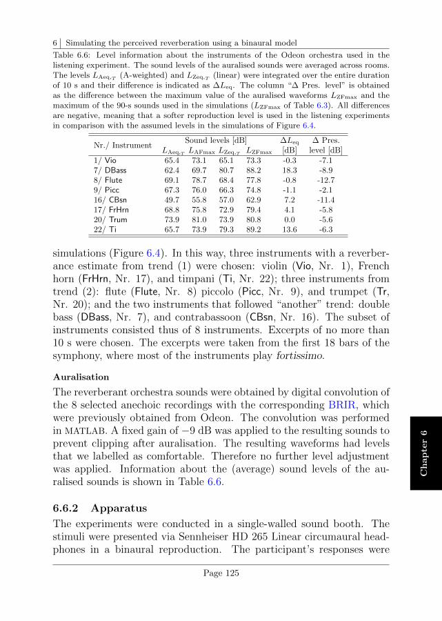
6 Simulating the perceived reverberation using a binaural model
Ch
ap
ter
6
Table 6.6: Level information about the instruments of the Odeon orchestra used in thelistening experiment. The sound levels of the auralised sounds were averaged across rooms.The levels LAeq,T (A-weighted) and LZeq,T (linear) were integrated over the entire durationof 10 s and their difference is indicated as ∆Leq. The column “∆ Pres. level” is obtainedas the difference between the maximum value of the auralised waveforms LZFmax and themaximum of the 90-s sounds used in the simulations (LZFmax of Table 6.3). All differencesare negative, meaning that a softer reproduction level is used in the listening experimentsin comparison with the assumed levels in the simulations of Figure 6.4.
Nr./ InstrumentSound levels [dB] ∆Leq ∆ Pres.
LAeq,T LAFmax LZeq,T LZFmax [dB] level [dB]1/ Vio 65.4 73.1 65.1 73.3 -0.3 -7.17/ DBass 62.4 69.7 80.7 88.2 18.3 -8.98/ Flute 69.1 78.7 68.4 77.8 -0.8 -12.79/ Picc 67.3 76.0 66.3 74.8 -1.1 -2.116/ CBsn 49.7 55.8 57.0 62.9 7.2 -11.417/ FrHrn 68.8 75.8 72.9 79.4 4.1 -5.820/ Trum 73.9 81.0 73.9 80.8 0.0 -5.622/ Ti 65.7 73.9 79.3 89.2 13.6 -6.3
simulations (Figure 6.4). In this way, three instruments with a reverber-ance estimate from trend (1) were chosen: violin (Vio, Nr. 1), Frenchhorn (FrHrn, Nr. 17), and timpani (Ti, Nr. 22); three instruments fromtrend (2): flute (Flute, Nr. 8) piccolo (Picc, Nr. 9), and trumpet (Tr,Nr. 20); and the two instruments that followed “another” trend: doublebass (DBass, Nr. 7), and contrabassoon (CBsn, Nr. 16). The subset ofinstruments consisted thus of 8 instruments. Excerpts of no more than10 s were chosen. The excerpts were taken from the first 18 bars of thesymphony, where most of the instruments play fortissimo.
Auralisation
The reverberant orchestra sounds were obtained by digital convolution ofthe 8 selected anechoic recordings with the corresponding BRIR, whichwere previously obtained from Odeon. The convolution was performedin MATLAB. A fixed gain of −9 dB was applied to the resulting sounds toprevent clipping after auralisation. The resulting waveforms had levelsthat we labelled as comfortable. Therefore no further level adjustmentwas applied. Information about the (average) sound levels of the au-ralised sounds is shown in Table 6.6.
6.6.2 Apparatus
The experiments were conducted in a single-walled sound booth. Thestimuli were presented via Sennheiser HD 265 Linear circumaural head-phones in a binaural reproduction. The participant’s responses were
Page 125

6 Simulating the perceived reverberation using a binaural model
collected using the software Web Audio Evaluation (WAE) (Jillings etal., 2016) using Google Chrome on a local computer.
6.6.3 Participants
Twenty-four participants (5 females and 19 males) were recruited fromthe JF Schouten subject database of the TU/e university. At the timeof testing, the participants were between 19 and 43 years old (average of24 years) and they all had self-reported normal hearing. They providedtheir informed consent before starting the experimental session and werepaid for their contribution.
The sample size of 24 participants was assessed a priori. The experi-ment uses a repeated measures (within-subject) design. It is of interest tocheck the main effects of two factors: “musical instrument” and “room”.The experiment considers 64 sound stimuli that can be grouped intoeither 8 groups of 8 instrument measurements or 8 groups of 8 roommeasurements. The first case is of more interest for us, with a null hy-pothesis that revereberance estimates are the same for the 8 instrumentmeasurements. Based on the simulations shown earlier in this chapter weexpect to reject this hypothesis. Assuming a medium effect size (Cohen’sf = 0.25), an α level (p-value) of 0.05 to support/reject the hypothesisand a power of 90%, 24 participants are required to reach the desiredeffect size (actual power of 0.96). This analysis was done in the softwareG*Power (Faul et al., 2007, 2009).
6.6.4 Experimental sessions
The experimental sessions were organised in a one-hour session per par-ticipant, including breaks. A multi-stimulus comparison method wasused, where the participant was presented with 8 stimuli that he or shehad to sort along a scale from 0 to 1 according to an increasing sensationof reverberance. Sixteen trials (i.e., 16 scales with 8 stimuli each) werepresented to each participant, with 8 trials having stimuli of the sameinstrument in different rooms (within-instrument), and 8 trials havingdifferent instruments in the same room (within-room).
6.7 Experimental results
6.7.1 Within-instrument evaluation
The experimental results for the within-instrument evaluations are shownin Figure 6.7. The median reverberance estimates PREV,exp vary between
Page 126
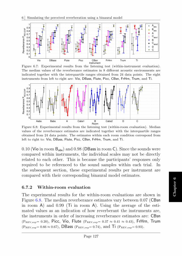
6 Simulating the perceived reverberation using a binaural model
Ch
ap
ter
6
Vio DBass Flute Picc CBsn FrHrn Trum Ti
0
0.1
0.2
0.3
0.4
0.5
0.6
0.7
0.8
0.9
1R
eve
rbe
ran
ce
PR
EV
,EX
P
Instrument
Aabs
Babs
A
Cabs1
B
Cabs2
D
C
Figure 6.7: Experimental results from the listening test (within-instrument evaluation).The median values of the reverberance estimates in 8 different acoustic environments areindicated together with the interquartile ranges obtained from 24 data points. The eightinstruments from left to right are: Vio, DBass, Flute, Picc, CBsn, FrHrn, Trum, and Ti.
Aabs Babs A Cabs1 B Cabs2 D C
0
0.1
0.2
0.3
0.4
0.5
0.6
0.7
0.8
0.9
1
Re
ve
rbe
ran
ce
PR
EV
,EX
P
Room
Figure 6.8: Experimental results from the listening test (within-room evaluation). Medianvalues of the reverberance estimates are indicated together with the interquartile rangesobtained from 24 data points. The estimates within each room condition correspond fromleft to right to: Vio, DBass, Flute, Picc, CBsn, FrHrn, Trum, and Ti.
0.10 (Vio in room Babs) and 0.98 (DBass in room C). Since the sounds werecompared within instruments, the individual scales may not be directlyrelated to each other. This is because the participants’ responses onlyrequired to be referenced to the sound samples within each trial. Inthe subsequent section, these experimental results per instrument arecompared with their corresponding binaural model estimates.
6.7.2 Within-room evaluation
The experimental results for the within-room evaluations are shown inFigure 6.8. The median reverberance estimates vary between 0.07 (CBsnin room A) and 0.99 (Ti in room A). Using the average of the esti-mated values as an indication of how reverberant the instruments are,the instruments in order of increasing reverberance estimates are: CBsn(PREV,exp= 0.20), Picc, Vio, Flute (PREV,exp= 0.37 ≈ 0.41 ≈ 0.43), FrHrn, Trum(PREV,exp= 0.66 ≈ 0.67), DBass (PREV,exp= 0.74), and Ti (PREV,exp= 0.93).
Page 127
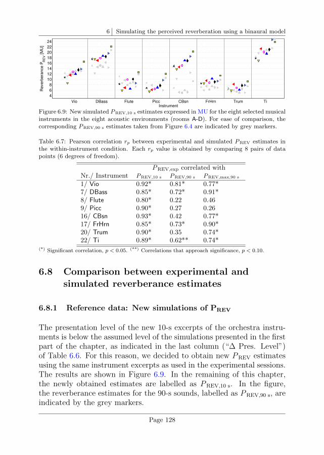
6 Simulating the perceived reverberation using a binaural model
Vio DBass Flute Picc CBsn FrHrn Trum Ti
4
6
8
10
12
14
16
18
20
22
24R
everb
era
nce P
RE
V [M
U]
Instrument
Figure 6.9: New simulated PREV,10 s estimates expressed in MU for the eight selected musicalinstruments in the eight acoustic environments (rooms A-D). For ease of comparison, thecorresponding PREV,90 s estimates taken from Figure 6.4 are indicated by grey markers.
Table 6.7: Pearson correlation rp between experimental and simulated PREV estimates inthe within-instrument condition. Each rp value is obtained by comparing 8 pairs of datapoints (6 degrees of freedom).
PREV,exp correlated withNr./ Instrument PREV,10 s PREV,90 s PREV,max,90 s
1/ Vio 0.92* 0.81* 0.77*7/ DBass 0.85* 0.72* 0.91*8/ Flute 0.80* 0.22 0.469/ Picc 0.90* 0.27 0.2616/ CBsn 0.93* 0.42 0.77*17/ FrHrn 0.85* 0.73* 0.90*20/ Trum 0.90* 0.35 0.74*22/ Ti 0.89* 0.62** 0.74*
(*) Significant correlation, p < 0.05. (**) Correlations that approach significance, p < 0.10.
6.8 Comparison between experimental andsimulated reverberance estimates
6.8.1 Reference data: New simulations of PREV
The presentation level of the new 10-s excerpts of the orchestra instru-ments is below the assumed level of the simulations presented in the firstpart of the chapter, as indicated in the last column (“∆ Pres. Level”)of Table 6.6. For this reason, we decided to obtain new PREV estimatesusing the same instrument excerpts as used in the experimental sessions.The results are shown in Figure 6.9. In the remaining of this chapter,the newly obtained estimates are labelled as PREV,10 s. In the figure,the reverberance estimates for the 90-s sounds, labelled as PREV,90 s, areindicated by the grey markers.
Page 128
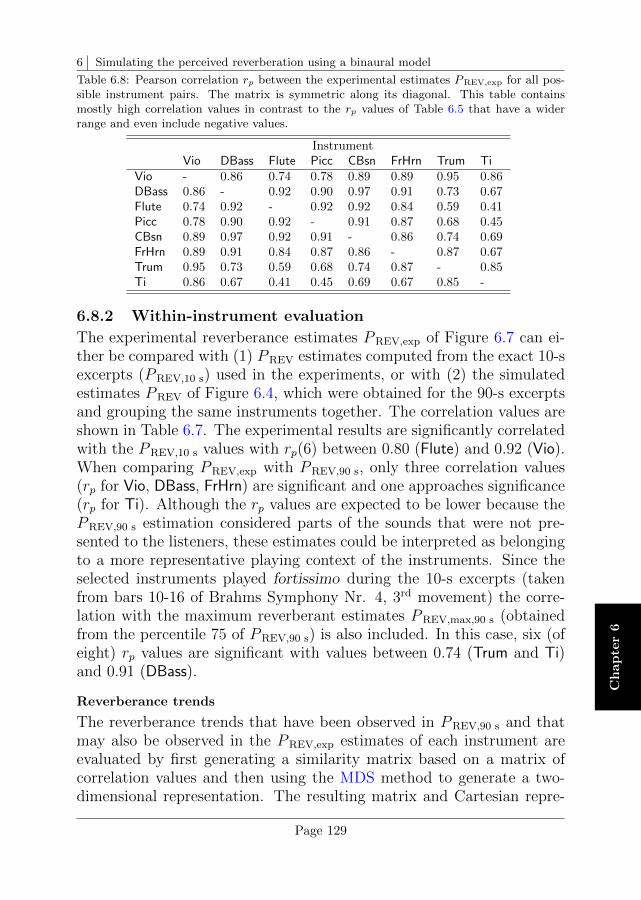
6 Simulating the perceived reverberation using a binaural model
Ch
ap
ter
6
Table 6.8: Pearson correlation rp between the experimental estimates PREV,exp for all pos-sible instrument pairs. The matrix is symmetric along its diagonal. This table containsmostly high correlation values in contrast to the rp values of Table 6.5 that have a widerrange and even include negative values.
InstrumentVio DBass Flute Picc CBsn FrHrn Trum Ti
Vio - 0.86 0.74 0.78 0.89 0.89 0.95 0.86DBass 0.86 - 0.92 0.90 0.97 0.91 0.73 0.67Flute 0.74 0.92 - 0.92 0.92 0.84 0.59 0.41Picc 0.78 0.90 0.92 - 0.91 0.87 0.68 0.45CBsn 0.89 0.97 0.92 0.91 - 0.86 0.74 0.69FrHrn 0.89 0.91 0.84 0.87 0.86 - 0.87 0.67Trum 0.95 0.73 0.59 0.68 0.74 0.87 - 0.85Ti 0.86 0.67 0.41 0.45 0.69 0.67 0.85 -
6.8.2 Within-instrument evaluation
The experimental reverberance estimates PREV,exp of Figure 6.7 can ei-ther be compared with (1) PREV estimates computed from the exact 10-sexcerpts (PREV,10 s) used in the experiments, or with (2) the simulatedestimates PREV of Figure 6.4, which were obtained for the 90-s excerptsand grouping the same instruments together. The correlation values areshown in Table 6.7. The experimental results are significantly correlatedwith the PREV,10 s values with rp(6) between 0.80 (Flute) and 0.92 (Vio).When comparing PREV,exp with PREV,90 s, only three correlation values(rp for Vio, DBass, FrHrn) are significant and one approaches significance(rp for Ti). Although the rp values are expected to be lower because thePREV,90 s estimation considered parts of the sounds that were not pre-sented to the listeners, these estimates could be interpreted as belongingto a more representative playing context of the instruments. Since theselected instruments played fortissimo during the 10-s excerpts (takenfrom bars 10-16 of Brahms Symphony Nr. 4, 3rd movement) the corre-lation with the maximum reverberant estimates PREV,max,90 s (obtainedfrom the percentile 75 of PREV,90 s) is also included. In this case, six (ofeight) rp values are significant with values between 0.74 (Trum and Ti)and 0.91 (DBass).
Reverberance trends
The reverberance trends that have been observed in PREV,90 s and thatmay also be observed in the PREV,exp estimates of each instrument areevaluated by first generating a similarity matrix based on a matrix ofcorrelation values and then using the MDS method to generate a two-dimensional representation. The resulting matrix and Cartesian repre-
Page 129
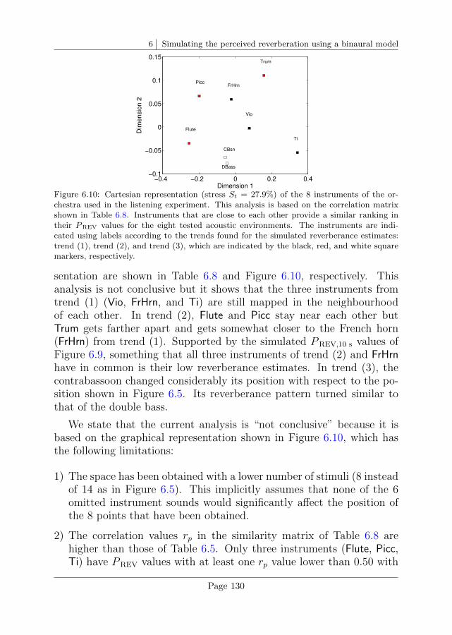
6 Simulating the perceived reverberation using a binaural model
−0.4 −0.2 0 0.2 0.4−0.1
−0.05
0
0.05
0.1
0.15
Vio
DBass
Flute
Picc
CBsn
FrHrn
Trum
Ti
Dimension 1
Dim
ensio
n 2
Figure 6.10: Cartesian representation (stress St = 27.9%) of the 8 instruments of the or-chestra used in the listening experiment. This analysis is based on the correlation matrixshown in Table 6.8. Instruments that are close to each other provide a similar ranking intheir PREV values for the eight tested acoustic environments. The instruments are indi-cated using labels according to the trends found for the simulated reverberance estimates:trend (1), trend (2), and trend (3), which are indicated by the black, red, and white squaremarkers, respectively.
sentation are shown in Table 6.8 and Figure 6.10, respectively. Thisanalysis is not conclusive but it shows that the three instruments fromtrend (1) (Vio, FrHrn, and Ti) are still mapped in the neighbourhoodof each other. In trend (2), Flute and Picc stay near each other butTrum gets farther apart and gets somewhat closer to the French horn(FrHrn) from trend (1). Supported by the simulated PREV,10 s values ofFigure 6.9, something that all three instruments of trend (2) and FrHrnhave in common is their low reverberance estimates. In trend (3), thecontrabassoon changed considerably its position with respect to the po-sition shown in Figure 6.5. Its reverberance pattern turned similar tothat of the double bass.
We state that the current analysis is “not conclusive” because it isbased on the graphical representation shown in Figure 6.10, which hasthe following limitations:
1) The space has been obtained with a lower number of stimuli (8 insteadof 14 as in Figure 6.5). This implicitly assumes that none of the 6omitted instrument sounds would significantly affect the position ofthe 8 points that have been obtained.
2) The correlation values rp in the similarity matrix of Table 6.8 arehigher than those of Table 6.5. Only three instruments (Flute, Picc,Ti) have PREV values with at least one rp value lower than 0.50 with
Page 130
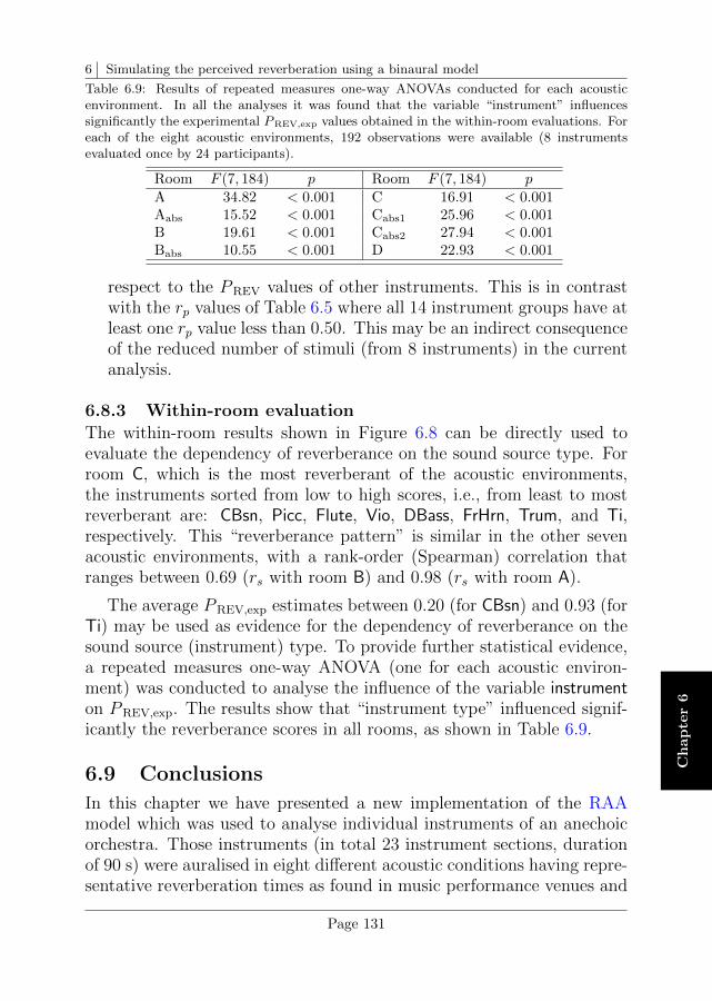
6 Simulating the perceived reverberation using a binaural model
Ch
ap
ter
6
Table 6.9: Results of repeated measures one-way ANOVAs conducted for each acousticenvironment. In all the analyses it was found that the variable “instrument” influencessignificantly the experimental PREV,exp values obtained in the within-room evaluations. Foreach of the eight acoustic environments, 192 observations were available (8 instrumentsevaluated once by 24 participants).
Room F (7, 184) p Room F (7, 184) pA 34.82 < 0.001 C 16.91 < 0.001Aabs 15.52 < 0.001 Cabs1 25.96 < 0.001B 19.61 < 0.001 Cabs2 27.94 < 0.001Babs 10.55 < 0.001 D 22.93 < 0.001
respect to the PREV values of other instruments. This is in contrastwith the rp values of Table 6.5 where all 14 instrument groups have atleast one rp value less than 0.50. This may be an indirect consequenceof the reduced number of stimuli (from 8 instruments) in the currentanalysis.
6.8.3 Within-room evaluation
The within-room results shown in Figure 6.8 can be directly used toevaluate the dependency of reverberance on the sound source type. Forroom C, which is the most reverberant of the acoustic environments,the instruments sorted from low to high scores, i.e., from least to mostreverberant are: CBsn, Picc, Flute, Vio, DBass, FrHrn, Trum, and Ti,respectively. This “reverberance pattern” is similar in the other sevenacoustic environments, with a rank-order (Spearman) correlation thatranges between 0.69 (rs with room B) and 0.98 (rs with room A).
The average PREV,exp estimates between 0.20 (for CBsn) and 0.93 (forTi) may be used as evidence for the dependency of reverberance on thesound source (instrument) type. To provide further statistical evidence,a repeated measures one-way ANOVA (one for each acoustic environ-ment) was conducted to analyse the influence of the variable instrumenton PREV,exp. The results show that “instrument type” influenced signif-icantly the reverberance scores in all rooms, as shown in Table 6.9.
6.9 Conclusions
In this chapter we have presented a new implementation of the RAAmodel which was used to analyse individual instruments of an anechoicorchestra. Those instruments (in total 23 instrument sections, durationof 90 s) were auralised in eight different acoustic conditions having repre-sentative reverberation times as found in music performance venues and
Page 131
6 Simulating the perceived reverberation using a binaural model
rehearsal rooms (0.8-2.5 s). We provide experimental evidence for thevalidity of the reverberance estimates PREV of the RAA model especiallyfor the case when the same instrument sound is compared in the differentacoustic environments.
The reverberance estimates (PREV) obtained from the RAA modelvaried depending on the spectral content of the analysed instrument andthe presentation level. At the same time, we found a large variation of theestimates when using a running analysis window within each individualinstrument. The simulated PREV values had a systematic relationshipwith EDT and T30 that could be classified in two different trends ex-plaining 91.3% of the simulated data. In 60.9% of the data, PREV hada higher correlation with EDT than with T30. This trend was found ininstruments with a balanced spectrum across critical bands. We couldnot provide conclusive evidence for the existence of those trends basedon the experimental results with 8 (of the 23) instruments. However,the experimental results provided evidence for (1) the significant influ-ence of the instrument type on the perceived reverberation, and (2) thevalidity of the simulated PREV estimates using sound excerpts that hada duration of 10 s. The simulated PREV estimates were all significantlycorrelated with the experimental estimates.
Further work is needed to quantify the extent to which reverberanceactually depends on the presentation level of the test sounds. In our ex-perimental approach, the presentation level of the instrument sounds wasnot varied, accounting only for natural level differences due to differentsound strength values in each of the acoustic environments. The investi-gation of this aspect will require further collection of experimental data.
The research presented in this chapter resulted from an exchange (sec-ondment) project at the acoustic consultancy company Muller-BBM.The research goals were: (1) to introduce perception-based predictionsof room acoustic indicators to real-world (room) acoustic conditions, and(2) to evaluate to what extent such an approach correlates with listen-ers’ experiences. The significant correlation between simulated and ex-perimental estimates of reverberance is therefore an encouraging resultindicating that perception-based predictors are not only of academic in-terest, but might also improve the predictions obtained in the context ofroom acoustic consultancy. However, one needs to be aware that suchpsychoacoustic-based approaches (see also Lee et al., 2012, 2017) repre-sent a fundamental change of paradigm in room acoustics. According
Page 132
6 Simulating the perceived reverberation using a binaural model
Ch
ap
ter
6
to established measurement guidelines (ISO, 2009), the acoustic proper-ties of a room are considered as (level) linear and time invariant, that is,room properties are assumed to be independent of the type of excitation,and of the level of the exciting signals. Such a source-filter characterisa-tion of room acoustic transmission allows to characterise rooms as lineartime-invariant (LTI) systems. The results of this chapter may be usedas evidence that the perception of room acoustic parameters (of rever-berance, in our case) depends on the context for which the room is usedand this is contrary to the idea of an LTI system.
Page 133


7 General discussion
The work presented in this thesis is concerned with the use of an auditorymodel for the evaluation of complex sounds, particularly musical instru-ments, with a special emphasis on the evaluation of perceptual similarityof individual notes played on different pianos. The following instrumentshave been evaluated: (1) the hummer (Chapter 2), which is a simple in-strument with sounds that oscillate in amplitude and frequency. Existingrecordings and synthesised sounds obtained from a physical model werecompared; (2) Recordings of one note played on different pianos (Chap-ter 3, 4, 5), and; (3) Existing recordings of an anechoic orchestra, towhich the effect of reverberation has been added by digital convolution,generating eight acoustic environments (Chapter 6).
In Chapter 2, sounds of the hummer in its acoustic modes 2 and 4were evaluated using a selection of psychoacoustic descriptors namelyloudness, loudness fluctuations, roughness, and fluctuation strength. Ananalysis based on fundamental frequency estimates was also included.The analyses were based on reported just-noticeable differences (JND)for each of the 5 evaluated descriptors. The results showed that thesynthesised sounds of the hummer are more similar to the recorded onesin acoustic mode 2 than in mode 4. In mode 2, two descriptors hada difference of less than one JND and one descriptor was just abovethe JND. In mode 4 only one descriptor had a difference of less thanone JND. An analysis based on 5 descriptors can be interpreted as ananalysis based on 5 “dimensions” that are assumed to be appropriate toevaluate the characteristics of the test sounds.
In Chapter 3 the perceptual similarity among recordings of one noteplayed on different historical Viennese pianos was evaluated. Using theconcept of JND, two sounds are perceptually similar along one explicit
Page 135
7 General discussion
“dimension” if they differ by less than one JND. In this chapter percep-tual similarity was approached more abstractly, by asking participantsto discriminate two sounds while modifying the degree of similarity be-tween them. The objective was to develop a method where the similaritybetween sounds can not only be assessed but also manipulated by using aspecifically generated noise. The noise used to manipulate the difficultyof the task follows the spectro-temporal properties of the sounds beingtested and is derived from a modified ICRA noise algorithm. The ex-perimental method, that we named instrument-in-noise, was comparedwith the method of triadic comparisons, which is a widely used methodto evaluate the similarity among stimuli. For similarity estimates using7 piano sounds, the correlation between the results of both methods wasrp(17) = −0.47, p = 0.04, and rs(19) = −0.64, p < 0.001. We concludedthat the instrument-in-noise method is a promising method to evaluatethe similarity between sounds.
In Chapter 4 the instrument-in-noise method is simulated using an ex-isting computational model of auditory processing. The auditory (PEMO)model developed by Dau et al. (1997a) was used. The model was de-scribed together with the choice of parameters for each of its stages.The model uses a back-end decision stage (central processor) that pro-cesses the outputs of the model, i.e., the internal representations of theincoming sounds. We developed a custom implementation of the centralprocessor to enable the artificial listener (i.e., the model) to estimate theamount of noise needed to correctly discriminate two piano sounds. Weused the same piano sounds and ICRA noises as in Chapter 3. The sim-ulated and experimental thresholds had a moderate to high correlationwith rp(17) = 0.54, p = 0.02, and rs(19) = 0.63, p < 0.001.
In Chapter 5 the instrument-in-noise method was further evaluatedusing the same set of piano sounds to which the reverberation of a largeroom (ground area of 570 m2 and EDT of 3.0 s at mid frequencies) wasadded by means of digital convolution. The instrument-in-noise methodwas evaluated experimentally (similar to Chapter 3) and by runningsimulations (similar to Chapter 4). The results of this chapter showedthat: (1) For the experimental data, thresholds of the instrument-in-noise method thresexp are correlated with the results of the experimentaltriadic comparisons with rp(18) = −0.49, p = 0.03, and rs(19) = −0.65,p < 0.001; (2) For the obtained instrument-in-noise thresholds, theexperimental thresexp and simulated thressim values are correlated withrp(18) = 0.58, p < 0.01, and rs(19) = 0.61, p < 0.001.
Page 136
7 General discussion
Ch
ap
ter
7
In Chapter 6, an example of the auditory modelling framework ap-plied to room acoustics is given. More specifically, a binaural auditory(RAA) model (van Dorp, 2011) is used to study the perceived reverber-ation (reverberance) of different instrument sounds in eight simulatedrooms. The RAA model has peripheral stages similar to the PEMOmodel that are applied independently to left- and right-ear signals, andthe central processor converts individual internal representations intoa metric of reverberance PREV. Listening experiments with 8 of theinstruments were conducted to test the validity of the RAA model ina within-instrument modality (same instrument evaluated in the eightrooms) and in a within-room evaluation (same room for eight differentinstruments). The results of the within-instrument evaluation showedthat PREV estimates are highly correlated with experimental estimateshaving rp(6) values ranging between 0.80 and 0.93. The experimental re-sults of the within-room evaluation showed that in all the environmentsthe instrument type (i.e., sound source type) influences significantly theparticipants’ reverberance scores. The extension of the use of the uni-fied modelling framework of Chapters 4 and 5 to this application by justadopting a different but “suitable” central processor stage shows thepotential of using psychoacoustic modelling in auditory tasks that aredifferent to those for which the models have been previously validated(see, e.g., Appendix D).
7.1 Advantages of the current auditory modellingapproach
Experience was gained on the perceptual modelling of a listening task,namely the instrument-in-noise method, that was designed to evaluatethe similarity among sounds (Chapter 3). Our implementation of thetask can provide interesting information about the sounds being evalu-ated. Some of these benefits are listed in this section.
The instrument-in-noise method was implemented to compare pairsof sounds using a 3-AFC task. An auditory model was used to produceinternal representations of the three sequentially-presented test intervalsupon which the artificial listener chose one as being (most likely) differ-ent to the other two test intervals. One of the primary advantages ofthis approach is, therefore, the possibility to algorithmically evaluateperceptual aspects of the sounds being compared.
One example of algorithmic evaluation was presented in Chapter 6.
Page 137
7 General discussion
In that chapter an existing auditory model was used to simulate theperceived reverberation (reverberance) elicited by a set of different in-strument sounds. In a listening experiment presented in the second partof the chapter we assumed that instrument sounds for which the “arti-ficial listener” provided similar reverberance estimates were also goingto be judged as similar by human listeners. Motivated by this idea,we chose a subset of 8 (of 23) instrument sounds for which the audi-tory model showed a characteristic reverberance performance (differenttrends). Hence, the model simulations (first part of the chapter) wereused as a way to obtain some “a priori” knowledge about human perfor-mance, helping with the design of the listening experiment.
Another interesting aspect of the internal representations obtainedfrom the auditory model is that they are multidimensional. The di-mensions of the representations are related to time, audio frequency,and modulation frequency. Therefore the current approach provides thepossibility to perform an advanced “sound feature analysis” based on in-formation available along either of those dimensions. Since the objectiveof this thesis was to use the auditory modelling framework in a similaritytask, our “advanced analysis” of the multidimensional piano representa-tions was used to investigate which cues along the three dimensions mayhave been used by the artificial listener (and potentially also by our par-ticipants) to judge the piano sounds, rather than looking at what physicalproperties of the piano sounds lead to such representations. A comple-mentary approach where piano sounds have been analysed in terms ofsound features is given by Chaigne, Osses, and Kohlrausch (2018). Inthat study, four of the C#5-piano sounds used in Chapter 3 (P4-P7)were evaluated together with recordings of other five notes (C2, F3, C4,A4, G6). A comparison between the results of our information-basedanalysis and their seven spectro-temporal descriptors may provide fur-ther insights into how the physical properties of the piano are actuallyrelated to perceptual aspects.
7.2 Limitations of the current approach
The auditory (PEMO) model has been applied to the specific case ofsimilarity between sounds (Chapter 4 and 5). We identified a number oflimitations of our approach that are related to (1) the choice of the audi-tory model, (2) the way the similarity task was implemented, and (3, 4)the way the information of the optimal detector was limited and reduced.
Page 138
7 General discussion
Ch
ap
ter
7
7.2.1 Choice of the model
The PEMO model used in this thesis has a level-independent critical-band filter bank (stage 2, ERB filter bank in Figure 4.1, page 56). Thisis in contrast to the non-linear behaviour (compressive characteristic) ofthe basilar membrane, which is more compressive towards higher frequen-cies (see, e.g., Saremi et al., 2016, their Figure 3). Given that we foundthe decision criterion of the piano discrimination with notes of the samepitch to rely mostly on a frequency region above F0, particularly between1000 and 3000 Hz, comprising about 4 harmonics of the note (see panel(a) of Figure 4.10, page 77), the use of a non-linear critical-band filterbank coupled to the auditory model would change the sensitivity of themodel to our piano samples, that would in turn affect the estimation ofsimulated thresholds. Our motivation to choose the PEMO model and,therefore, the Gammatone filter bank came from our higher degree ofsuccess in replicating simulated data reported in the literature comparedwith more recent versions of the auditory model.
The PEMO model was used as a monaural model despite the factthat the piano sounds were presented diotically (Chapter 3) and binau-rally (Chapter 5) to the participants. We would not expect significantchanges between monaural and diotic discrimination thresholds (see, e.g.,Langhans & Kohlrausch, 1992) and although we did not use the right-earchannels of the piano sounds in the simulations of Chapter 5, we wouldexpect that similar discrimination cues are available with respect to theuse of the left-ear channel. In order to further apply the PEMO modelto other auditory tasks it is important to evaluate the role of processingleft and right-ear signals in parallel and by coupling their internal repre-sentations to have access to binaural cues as Breebaart et al. (2001) did.The use of the PEMO model in such a context would allow the use ofmodulation-frequency information for simulating binaural tasks.
7.2.2 Implementation of the similarity task
The similarity task was implemented as a 3-AFC discrimination experi-ment. With this approach, the test sounds are presented sequentiallyto the participants and the similarity assessment is based on the com-parison of individual piano notes that have the same F0 and thesame duration. Due to the implementation of the task as sequentially-presented intervals, a simple top-down approach (memory templates)could be adopted, assuming that the participant is able to “learn” anduse this information always in the best possible way. In practice, this
Page 139
7 General discussion
represents a situation where the participant is recursively exposed andgets familiar with the sounds. Hence, the presentation of sounds as in-dividual notes represents a condition where the participant can focus onsmaller sound differences compared to, e.g., melodic lines with multi-ple notes (and/or multiple instruments) where there is less exposure toone individual note (and/or instrument). In that case a more elaboratetop-down approach would be needed. Such an approach should use somesort of information weighting that may be influenced by attention and/orsaliency aspects.
7.2.3 Additive internal noiseThe internal noise was used to limit the artificial listener’s performancein an intensity-discrimination task (see Appendix D). The use of sucha simple additive internal noise was found to be not accurate enoughin simulations of several AM detection tasks (Ewert & Dau, 2004). Toovercome this limitation, Wallaert, Moore, Ewert, and Lorenzi (2017)adopted a multiplied noise as an additional source of internal variabilitybesides the additive internal noise and a memory noise they used toreduce the memory capacity of the model (that can be compared withour use of tobs).
7.2.4 Reduction of information in the optimal detectorThe artificial listener was found to be too sensitive to differences in thestimuli when considering whole-duration piano waveforms with tobs du-rations of 1.5 and 2.2 s in Chapters 4 and 5, respectively. As a way toreduce available cues in the model, shorter observation durations tobs
were evaluated with as result tobs values of 0.25 and 0.20 s. We did notevaluate other forms of information reduction such as the applicationof (additional) smoothing to the internal representations or the use ofa temporal weighting that could provide a higher emphasis to the in-formation present in the first 0.20-0.25 s with respect to the rest of therepresentation instead of removing the latter one completely.
7.3 Perspectives for further research
The modelling framework used in this thesis includes stages of peripheralprocessing of the auditory system and provides the possibility to add aback-end stage or central processor. To apply such an approach to asimilarity task involving piano sounds we had to (1) choose the appro-priate parameters to be used in the peripheral processing part, and to
Page 140
7 General discussion
Ch
ap
ter
7
(2) adjust the central processor in a way that two or more sound (in-ternal) representations could be conveniently compared to each other toassess how similar they are. This corresponds to a very general approachand we believe that it can be applied to many other applications as longas “hearing” is involved. We give next two examples of potential ap-plications, one related to room acoustics and another related to humanecholocation. For both examples it would be desirable to use the audi-tory model in a binaural set-up, using a suitable coupling of left andright-ear internal representations in the central processor.
The first example of application was actually given in Chapter 6 wherea binaural model (the RAA model) was used to investigate the reverber-ance of different sound sources in room acoustics. The particular con-text in which that chapter was developed was a consequence of a jointproject with the acoustic consultancy company Muller-BBM. The goalof the project was to use an existing binaural model in the evaluation ofrecorded (auralised) sounds in different rooms, evaluating to what extentreverberance estimates from the model correlate with physical measure-ments of reverberation time using standardised procedures (ISO, 2009).Our goal was, therefore, to evaluate how well did the (existing) RAAmodel perform rather than pursuing an improvement of the simulationpower of that model. The use of this psychoacoustic-based model sug-gests a change in paradigm in room acoustics. The ISO procedures en-courage the characterisation of an acoustic environment independent ofthe sound source and its level, which is in contrast to the approach of us-ing the RAA model along with, e.g., the use of loudness-based reverbera-tion estimates (Lee et al., 2012). In this context, we suggest two possibleways to further extend the use of the binaural RAA model: (1) To inves-tigate the dependency of reverberance on the presentation level of thestimuli. This is motivated by the strong level dependency that weidentified in the model –also recently reported by Lee et al. (2017)– andrequires further experimental evidence; and (2) to extend the validationof the RAA model to other room acoustics parameters, such as clarity,listener envelopment, and apparent source width (van Dorp, 2011; vanDorp et al., 2013) using more sound sources.
Our second example of potential application is the use of (binaural)auditory modelling to study human echolocation. Echolocation is a per-ceptual ability mostly used by blind people to explore a given spatialenvironment. Sounds that are emitted orally (“source”) are normallyused by them to extract information about surrounding objects (in a
Page 141
7 General discussion
“medium”) based on the spectral and spatial cues conveyed in the soundsthat are heard back (“receiver”). Experiments on human echolocationhave been mostly implemented as performance tasks (see, e.g., Dufouret al., 2005; Guzman, 2016; Rowan et al., 2017) which, based on thearguments presented in the introduction of this thesis, is an auspiciouscondition to be simulated by means of auditory models. Two types ofecholocation tasks are the localisation of an object and the discrimina-tion of the size of an object (de Vos & Hornikx, 2018). Data from suchtasks analysed using an information-based approach of the underlyinginternal representations as used in Chapters 4 and 5 may provide usefulinsights to optimise the “sound source” by, e.g., developing artificiallygenerated (optimal) clicks, or to optimise the “medium” by designingrooms that enhance the transmission of spectral and spatial cues.
7.4 General conclusionThe main goal of this thesis was to gain insights into the perceptual mod-elling of “an” auditory task. We focused our efforts on the perceptualsimilarity of a specific note (C#5) played on a set of 7 historical Vien-nese pianos by using an auditory model. For doing this we developed amethod where the similarity between two sounds could be manipulatedby using noise, allowing to evaluate similarity as a performance task.The method, that we named instrument-in-noise, was compared withthe method of triadic comparisons reaching moderate to high correla-tions using the piano sounds in two acoustic conditions: “anechoic” andreverberant (EDT of 3 s). An existing modelling approach based on amodel of the effective processing in the auditory system was used. Thesimulated thresholds thressim were in both cases highly correlated withthe experimental thresholds thresexp, but they had a strong “primacy”effect, where only the first 0.25 or 0.20 s of the internal representationswere used to produce these results. The encouraging results of our mod-elling approach allowed us to perform information-based analyses on thepiano internal representations. We concluded that the weighting of in-formation used by the artificial listener may be similar to that used byhuman listeners. The advantages and limitations of both experimentaland modelling approach were discussed. Due to the use of the unifiedauditory modelling framework offered by the adopted model, further re-search is suggested in applications involving binaural listening, whichrepresents a different type of auditory task to that implemented here forthe perceptual similarity between stimuli.
Page 142
References
Agus, T., Suied, C., Thorpe, S., & Pressnitzer, D. (2012). Fast recog-nition of musical sounds based on timbre. J. Acoust. Soc. Am., 131 (5),4124–4133.
Aures, W. (1985). Ein Berechnungsverfahren der Rauhigkeit. Acustica,58 (5), 268–281.
Beranek, L. (2004). Concert halls and opera houses: Music, acousticsand architecture. Springer New York.
Boersma, P. (1993). Accurate short-term analysis of the fundamentalfrequency and the harmonics-to-noise ratio of a sampled sound. Pro-ceedings of the Institute of Phonetic Sciences , 17 , 97–110.
Boersma, P., & Weenink, D. (2001). Praat, a system for doing phoneticsby computer. Glot Int., 5 (9/10), 341–345.
Bradley, R. (1953). Some statistical methods in taste testing and qualityevaluation. Biometrics , 9 (1), 22–38.
Breebaart, J., van de Par, S., & Kohlrausch, A. (2001). Binauralprocessing model based on contralateral inhibition. I. Model structure.J. Acoust. Soc. Am., 110 (2), 1074–1088.
Burton, M., & Nerlove, S. (1976). Balanced designs for triads tests:Two examples from English. Social Science Research, 5 , 247–267.
Carroll, J., & Chang, J. (1970). Analysis of individual differences inmultidimensional scaling via an N-way generalization of Eckart-Youngdecomposition. Psychometrika, 35 (3), 283–319.
Chabassier, J., Chaigne, A., & Joly, P. (2013). Modeling and simulationof a grand piano. J. Acoust. Soc. Am., 134 (1), 648–65.
Page 143
Chaigne, A. (2016). Acoustics of pianos: An historical perspective. InInternational Symposium on Musical and Room Acoustics. La Plata.
Chaigne, A., Hennet, M., Chabassier, J., & Durufle, M. (2016). Com-parison between three different Viennese pianos of the nineteenth cen-tury. In International Congress on Acoustics. Buenos Aires.
Chaigne, A., Osses, A., & Kohlrausch, A. (2018). Similarity of pianotones: a psychoacoustical and sound analysis study. Applied Acoustics(submitted).
Chalupper, J., & Fastl, H. (2002). Dynamic loudness model (DLM) fornormal and hearing-impaired listeners. Acta Acust. united Ac., 88 (3),378–386.
Chelazzi, L., Miller, E., Duncan, J., & Desimone, R. (1993). A neuralbasis for visual search in inferior temporal cortex. Nature, 363 , 345.
Daniel, P., & Weber, R. (1997). Psychoacoustical roughness: Implemen-tation of an optimized model. Acustica - Acta Acustica, 83 , 113–123.
Dau, T., Kollmeier, B., & Kohlrausch, A. (1997a). Modeling audi-tory processing of amplitude modulation. I. Detection and masking withnarrow-band carriers. J. Acoust. Soc. Am., 102 (5), 2892–2905.
Dau, T., Kollmeier, B., & Kohlrausch, A. (1997b). Modeling auditoryprocessing of amplitude modulation. II. Spectral and temporal integra-tion. J. Acoust. Soc. Am., 102 (5), 2906–2919.
Dau, T., Puschel, D., & Kohlrausch, A. (1996a). A quantitative modelof the “effective” signal processing in the auditory system. I. Modelstructure. J. Acoust. Soc. Am., 99 (6), 3615–3622.
Dau, T., Puschel, D., & Kohlrausch, A. (1996b). A quantitative modelof the “effective” signal processing in the auditory system. II. Simula-tions and measurements. J. Acoust. Soc. Am., 99 (6), 3623–3631.
Dau, T., Verhey, J., & Kohlrausch, A. (1999). Intrinsic envelope fluctu-ations and modulation-detection thresholds for narrow-band noise car-riers. J. Acoust. Soc. Am., 106 (5), 2752–2760.
De Man, B., & Reiss, J. (2013). A pairwise and multiple stimuli ap-proach to perceptual evaluation of microphone types. In Audio Engi-neering Society Convention 134. Rome, Italy.
Page 144
De Man, B., & Reiss, J. (2014). APE: Audio Perceptual EvaluationToolbox for MATLAB. In Audio Engineering Society Convention 136.Berlin, Germany.
de Leeuw, J., & Mair, P. (2009). Multidimensional scaling using ma-jorization. J. Stati. Softw., 31 (3), 1–30.
Derveaux, G., Chaigne, A., Joly, P., & Becache, E. (2003). Time-domain simulation of a guitar: Model and method. J. Acoust. Soc.Am., 114 (6), 3368–3383.
de Vos, R., & Hornikx, M. (2018). Human ability to judge relativesize and lateral position of a sound reflecting board using click signals:Influence of source position and click properties. Acta Acust. united Ac.,104 , 131–144.
Dreschler, W., Verschuure, H., Ludvigsen, C., & Westermann, S. (2001).ICRA noises: Artificial noise signals with speech-like spectral and tem-poral properties for hearing instrument assessment. Int. J. Audiol.,40 (3), 148–157.
Drullman, R., Festen, J., & Plomp, R. (1994). Effect of temporalenvelope smearing on speech reception. J. Acoust. Soc. Am., 95 , 1053.
Dubois, D. (2000). Categories as acts of meaning: The case of categoriesin olfaction and audition. Cognitive Science Quarterly , 1 , 35–68.
Dufour, A., Despres, O., & Candas, V. (2005). Enhanced sensitivity toecho cues in blind subjects. Exp. Brain Res., 165 , 515–519.
Ellis, D. (2002). A phase vocoder in MATLAB. Retrieved from http://
www.ee.columbia.edu/~dpwe/resources/matlab/pvoc/
Everitt, B. (2005). Multidimensional scaling and correspondence anal-ysis. In An R and S-PLUS companion to multivariate analysis (pp.91–114). Springer Verlag.
Ewert, S. (2013). AFC - A modular framework for running psychoacous-tic experiments and computational perception models. In Proceedings ofthe International Conference on Acoustics AIA-DAGA (pp. 1326–29).
Ewert, S., & Dau, T. (2000). Characterizing frequency selectivity forenvelope fluctuations. J. Acoust. Soc. Am., 108 (3), 1181–1196.
Page 145
Ewert, S., & Dau, T. (2004). External and internal limitations inamplitude-modulation processing. J. Acoust. Soc. Am., 116 (1), 478–490.
Fastl, H. (1977). Roughness and temporal masking patterns of sinu-soidally amplitude-modulated broadband noise. In E. Evans & J. Wilson(Eds.), Psychophysics and physiology of hearing (pp. 403–417). Aca-demic Press.
Fastl, H. (1982). Fluctuation strength and temporal masking patternsof amplitude-modulated broadband noise. Hear. Res., 8 (1), 59–69.
Fastl, H. (1983). Fluctuation strength of modulated tones and broad-band noise. In Hearing - physical bases and psychophysics (pp. 282–288).
Fastl, H., & Zwicker, E. (2007). Psychoacoustics, Facts and Models(Third ed.). Springer Berlin Heidelberg.
Faul, F., Erdfelder, E., Buchner, A., & Lang, A.-G. (2009). Statisticalpower analyses using G*Power 3.1: Tests for correlation and regressionanalyses. Behavior Research Methods , 41 (4), 1149–1160.
Faul, F., Erdfelder, E., Lang, A.-G., & Buchner, A. (2007). G*Power 3:A flexible statistical power analysis program for the social, behavioral,and biomedical sciences. Behav. Res. Methods , 39 (2), 175–191.
Fog, C., & Ballinger, R. (2008). A new symphonic hall, MusikhusetAarhus, Denmark. In Proceedings of acoustics 08 paris (pp. 363–368).
Francart, T., van Wieringen, A., & Wouters, J. (2008). APEX 3: amulti-purpose test platform for auditory psychophysical experiments.J. Neurosci. Meth., 172 (2), 283–93.
Fritz, C., Cross, I., Moore, B., & Woodhouse, J. (2007). Perceptualthresholds for detecting modifications applied to the acoustical proper-ties of a violin. J. Acoust. Soc. Am., 122 (6), 3640–3650.
Fritz, C., & Dubois, D. (2015). Perceptual evaluation of musical instru-ments: state of the art and methodology. Acta Acust. united Ac., 101 ,369–381.
Fritz, C., Woodhouse, J., Cheng, F., Cross, I., Blackwell, A., & Moore,B. (2010). Perceptual studies of violin body damping and vibrato. J.Acoust. Soc. Am., 127 (1), 513–524.
Page 146
Garcıa, R. (2015). Modelling the sensation of fluctuation strength (Mas-ter thesis). Eindhoven University of Technology.
Genuit, K. (1997). Background and practical examples of sound design.Acustica - Acta Acustica, 83 (5), 805–812.
Glasberg, B., & Moore, B. (1990). Derivation of auditory filter shapesfrom notched-noise data. Hear. Res., 47 , 103–138.
Glasberg, B., & Moore, B. (2002). A model of loudness applicable totime-varying sounds. J. Audio Eng. Soc., 50 (5), 331–342.
Goode, R., Killion, M., Nakamura, K., & Nishihara, S. (1994). Newknowledge about the function of the human middle ear: Developmentof an improved analog model. Am. J. Otol., 15 (2), 145–154.
Green, D., & Swets, J. (1966). Signal detection theory and psy-chophysics. John Wiley & Sons Inc.
Greenwood, D. (1990). A cochlear frequency position function forseveral species–29 years later. J. Acoust. Soc. Am., 87 (6), 2592–2605.
Grey, J. (1977). Multidimensional perceptual scaling of musical timbres.J. Acoust. Soc. Am., 61 (5), 1270–1277.
Grey, J. (1978). Timbre discrimination in musical patterns. J. Acoust.Soc. Am., 64 (2), 467–472.
Grey, J., & Gordon, J. (1978). Perceptual effects of spectral modifica-tions on musical timbres. J. Acoust. Soc. Am., 63 (5), 1493–1500.
Guastavino, C., & Katz, B. (2004). Perceptual evaluation of multi-dimensional spatial audio reproduction. J. Acoust. Soc. Am., 116 (2),1105–1115.
Guzman, R. (2016). The effects of multiple sound reflections on hu-man echolocation: Acoustical analysis of binaural cues in different rooms(Master thesis). University of Southampton.
Hansen, M., & Kollmeier, B. (2000). Objective modeling of speechquality with a psychoacoustically validated auditory model. J. AudioEng. Soc., 14 (6), 395–409.
Hirschberg, M., Rudenko, O., Nakiboglu, G., Holten, A., Willems, J.,& Hirschberg, A. (2013). The voice of the mechanical dragon. InProceedings of SMAC. Stockholm.
Page 147
Hohmann, V. (2002). Frequency analysis and synthesis using a Gam-matone filterbank. Acust. Acta Acust., 88 (3), 433–442.
Holube, I., & Kollmeier, B. (1996). Speech intelligibility predictionin hearing-impaired listeners based on a psychoacoustically motivatedperception model. J. Acoust. Soc. Am., 100 (3), 1703–1716.
Houtsma, A., Rossing, T., & Wagenaars, W. (1987). Auditory demon-strations. Eindhoven: Acoustical Society of America.
Huber, R., & Kollmeier, B. (2006). PEMO-Q—A new method forobjective audio quality assessment using a model of auditory perception.IEEE Trans. Audio, Speech, Lang. Process., 14 (6), 1902–1911.
ISO. (2009). ISO 3382-1:2009. Acoustics. Measurement of room acousticparameters – Part 1: Performance spaces.
ITU-R. (2015). BS.1534-3: Method for the subjective assessment ofintermediate quality level of coding systems.
Jepsen, M., Ewert, S., & Dau, T. (2008). A computational model ofhuman auditory signal processing and perception. J. Acoust. Soc. Am.,124 (1), 422–438.
Jillings, N., De Man, B., Moffat, D., Reiss, J., & Stables, R. (2016).Web Audio Evaluation Tool: A framework for subjective assessment ofaudio. 2nd Web Audio Conference.
Jørgensen, S., & Dau, T. (2011). Predicting speech intelligibility basedon the signal-to-noise envelope power ratio after modulation-frequencyselective processing. J. Acoust. Soc. Am., 130 (3), 1475–1487.
Kates, J., & Arehart, K. (2014). The hearing-aid speech quality index(HASQI) version 2. J Audio Eng. Soc., 62 , 99–117.
Kemp, S. (1982). Roughness of frequency-modulated tones. Acustica,50 , 126–133.
Kingdom, F., & Prins, N. (2016). Psychophysics: A practical introduc-tion (2nd ed.). Elsevier.
Klockgether, S., & van de Par, S. (2014). A Model for the Prediction ofRoom Acoustical Perception based on the Just Noticeable Differencesof Spatial Perception. Acta Acust. united Ac., 100 , 964–971.
Page 148
Klockgether, S., & van de Par, S. (2016). Just noticeable differences ofspatial cues in echoic and anechoic acoustical environments. J. Acoust.Soc. Am., 140 (4), EL352–EL357.
Kohlrausch, A., Braasch, J., Kolossa, D., & Blauert, J. (2013). An intro-duction to binaural processing. In The technology of binaural listening(pp. 1–32). Springer Berlin Heidelberg.
Kohlrausch, A., Fassel, R., & Dau, T. (2000). The influence of carrierlevel and frequency on modulation and beat-detection thresholds forsinusoidal carriers. J. Acoust. Soc. Am., 108 (2), 723–734.
Kohlrausch, A., Hermes, D., & Duisters, R. (2005). Modeling roughnessperception for sounds with ramped and damped temporal envelopes.Forum Acusticum(1), 1719–1724.
Kohlrausch, A., Puschel, D., & Alphei, H. (1992). Temporal reso-lution and modulation analysis in models of the auditory system. InM. Schouten (Ed.), The auditory processing of speech (Vol. 10, pp. 85–98). Mouton de Gruyter.
Kruskal, J. (1964a). Multidimensional scaling by optimizing goodnessof fit to a nonmetric hypothesis. Psychometrika, 29 (1), 1–27.
Kruskal, J. (1964b). Nonmetric multidimensional scaling: a numericalmethod. Psychometrika, 29 (2), 115–129.
Langhans, A., & Kohlrausch, A. (1992). Differences in auditory perfor-mance between monaural and dichotic conditions. I: masking thresholdsin frozen noise. J. Acoust. Soc. Am., 91 (6), 3456–3470.
Langner, G., & Schreiner, C. (1988). Periodicity coding in the InferiorColliculus of the cat. I. Neuronal mechanisms. J. Neurophysiol., 60 (6),1799–1822.
Lee, D., Cabrera, D., & Martens, W. (2012). The effect of loudnesson the reverberance of music: Reverberance prediction using loudnessmodels. J. Acoust. Soc. Am., 131 (2), 1194–1205.
Lee, D., van Dorp, J., Cabrera, D., & Qiu, X. (2017). Comparisonof psychoacoustic-based reverberance parameters. J. Acoust. Soc. Am.,142 (4), 1832–1840.
Page 149
Leong, V., Stone, M. a., Turner, R., & Goswami, U. (2014). A role foramplitude modulation phase relationships in speech rhythm perception.J. Acoust. Soc. Am., 136 (1), 366–381.
Levelt, W., van de Geer, J., & Plomp, R. (1966). Triadic comparisonsof musical intervals. Br. J. Math. Stat. Psychol., 19 , 163–179.
Levitt, H. (1971). Transformed up-down methods in psychoacoustics.J. Acoust. Soc. Am., 49 (2), 467–477.
Lopez-Poveda, E., & Meddis, R. (2001). A human nonlinear cochlearfilterbank. J. Acoust. Soc. Am., 110 (6), 3107–3118.
Mao, J., & Carney, L. (2015). Tone-in-noise detection using envelopecues: Comparison of signal-processing-based and physiological models.J. Assoc. Res. Otolaryngol., 16 (1), 121–133.
McAdams, S., & Bigand, E. (Eds.). (1993). Thinking in sound: Thecognitive psychology of human audition. Oxford University Press.
Meddis, R., & Hewitt, M. (1991). Virtual pitch and phase sensitivityof a computer model of the auditory periphery. I: Pitch identification.J. Acoust. Soc. Am., 89 (6), 2866–2882.
Meddis, R., & O’Mard, L. (1997). A unitary model of pitch perception.J. Acoust. Soc. Am., 102 (3), 1811–1820.
Meyer, J. (2009). Acoustics and the performance of music. Springer.
Miller, G. (1947). Sensitivity to changes in the intensity of white noiseand its relation to masking and loudness. J. Acoust. Soc. Am., 19 , 609.
Moore, B. (2003). Temporal integration and context effects in hearing.J. Phonetics , 31 , 563–574.
Moore, B., & Glasberg, B. (1983). Suggested formulae for calculatingauditory-filter bandwidths and excitation patterns. J. Acoust. Soc. Am.,74 (3), 750–753.
Moore, B., & Sek, A. (1992). Detection of combined frequency andamplitude modulation. J. Acoust. Soc. Am., 92 (6), 3119–3131.
Munkner, S. (1993). Modellentwicklung und Messungen zurWahrnehmung nichtstationarer akustischer Signale (Ph.D. thesis). Uni-versity of Gottingen.
Page 150
Nakiboglu, G., Rudenko, O., & Hirschberg, A. (2012). Aeroacousticsof the swinging corrugated tube: Voice of the Dragon. J. Acoust. Soc.Am., 131 (1), 749–765.
Novello, A., McKinney, M., & Kohlrausch, A. (2011). Perceptual evalu-ation of inter-song similarity in Western popular music. Journal of NewMusic Research, 40 (1), 1–26.
Osses, A., Garcıa, R., & Kohlrausch, A. (2016). Modelling the sensationof fluctuation strength. Proc. Mtgs. Acoust., 28 (050005), 1–8.
Patel, A., Iversen, J., & Rosenberg, J. (2006). Comparing the rhythmand melody of speech and music: the case of British English and French.J. Acoust. Soc. Am., 119 (5), 3034–3047.
Patterson, R. (1976). Auditory filter shapes derived with noise stimuli.J. Acoust. Soc. Am., 59 (3), 640–654.
Pralong, D., & Carlile, S. (1996). The role of individualized headphonecalibration for the generation of high fidelity virtual auditory space. J.Acoust. Soc. Am., 100 (6), 3785–3793.
Puschel, D. (1988). Prinzipien der zeitlichen der Analyse beim Horen(Ph.D. thesis). University of Gottingen.
Raake, A., Wierstorf, H., & Blauert, J. (2014). A case for TWO!EARSin audio quality assessment. In Forum Acusticum (pp. 1–10). Krakow.
Rabinowitz, W. (1970). Frequency and intensity resolution in audition(Master thesis). Massachusetts Institute of Technology.
Rindel, J. (2015). Orchestra simulation and auralisa-tion. Odeon. Retrieved from http://www.odeon.dk/pdf/
Application note Orchestra auralisation.pdf
Robles, L., & Ruggero, M. (2001). Mechanics of the mammalian cochlea.Physiol. Rev., 81 (3), 1305–1352.
Rosen, S. (1992). Temporal information in speech: acoustic, auditoryand linguistic aspects. Phil.Trans. R. Soc. London, 336 , 367–373.
Rowan, D., Papadopoulos, T., Archer, L., Goodhew, A., Cozens, H.,Guzman, R., Edwards, D., Holmes, H., & Allen, R. (2017). The de-tection of virtual objects using echoes by humans: Spectral cues. Hear.Res., 350 , 205–216.
Page 151
Saitis, C., Fritz, C., Guastavino, C., & Scavone, G. (2013). Conceptu-alization of violin quality by experienced performers. In Proceedings ofSMAC (pp. 123–128). Stockholm.
Saitis, C., Fritz, C., Scavone, G., Guastavino, C., & Dubois, D. (2017).Perceptual evaluation of violins: A psycholinguistic analysis of prefer-ence verbal descriptions by experienced musicians. J. Acoust. Soc. Am.,141 (4), 2746–2757.
Saldanha, E., & Corso, J. (1964). Timbre cues and the identification ofmusical instruments. J. Acoust. Soc. Am., 36 , 2021–2026.
Saremi, A., Beutelmann, R., Dietz, M., Ashida, G., Kretzberg, J., &Verhulst, S. (2016). A comparative study of seven human cochlear filtermodels. J. Acoust. Soc. Am., 140 (3), 1618–1634.
Schlittmeier, S. J., Weissgerber, T., Kerber, S., Fastl, H., & Hellbruck,J. (2012). Algorithmic modeling of the irrelevant sound effect (ISE) bythe hearing sensation fluctuation strength. Atten. Percept. Psychophys.,74 (1), 194–203.
Schroeder, M. (1968). Reference signal for signal quality studies. J.Acoust. Soc. Am., 44 (6), 1735–1736.
Shannon, R., Zeng, F., Kamath, V., Wygonski, J., & Ekelid, M. (1995).Speech recognition with primarily temporal cues. Science, 270 (5234),303–304.
Shepard, R. (1962). The analysis of proximities: multidimensionalscaling with an unknown distance function. I. Psychometrika, 27 (2),125–140.
Shepard, R. (1987). Toward a universal law of generalization for psy-chological science. Science, 237 (4820), 1317–1323.
Søndergaard, P., & Majdak, P. (2013). The Auditory Modeling Toolbox.In J. Blauert (Ed.), The technology of binaural listening (pp. 33–56).Springer Berlin Heidelberg.
Sontacchi, A. (1998). Entwicklung eines Modulkonzeptes fur die psy-choakustische Gerauschanalyse unter MATLAB (Unpublished doctoraldissertation). Technischen Universitat Graz.
Steeneken, H. (1992). On measuring and predicting speech intelligibility(Ph.D. thesis). University of Amsterdam.
Page 152

Stevens, S. (1955). The measurement of loudness. J. Acoust. Soc. Am.,27 (5), 815–829.
Stevens, S. (1956). The direct estimation of sensory magnitudes–loudness. Am. J. Psychol., 69 (1), 1–25.
Tahvanainen, H., Patynen, J., Lokki, T., Tahvanainen, H., Patynen, J.,& Lokki, T. (2015). Studies on the perception of bass in four concerthalls. Psychomusicology: Music, Mind, and Brain, 25 (3), 294–305.
Teret, E., Pastore, T., & Braasch, J. (2017). The influence of signal typeon perceived reverberance. J. Acoust. Soc. Am., 141 (3), 1675–1682.
Terhardt, E. (1978). Psychoacoustic evaluation of musical sounds. Per-ception & Psychophysics , 23 (6), 483–92.
Terhardt, E. (1979). Calculating virtual pitch. Hear. Res., 1 , 155–182.
van de Par, S., & Kohlrausch, A. (1995). Analytical expressions forthe envelope correlation of narrow-band stimuli. J. Acoust. Soc. Am.,98 (6), 3157–3169.
van Dorp, J. (2011). Auditory modelling for assessing room acoustics(Ph.D. thesis). Technische Universiteit Delft.
van Dorp, J., de Vries, D., & Lindau, A. (2013). Deriving content-specific measures of room acoustic perception using a binaural, nonlin-ear auditory model. J. Acoust. Soc. Am., 133 (3), 1572–1585.
van Veen, T., & Houtgast, T. (1983). On the perception of spectralmodulations. In Hearing - physical bases and psychophysics (p. 277).
Vogel, A. (1975). Uber den Zusammenhang zwischen Rauhigkeit undModulationsgrad (On the relation between roughness and degree ofmodulation). Acustica, 32 (5), 300–306.
von Klitzing, R., & Kohlrausch, A. (1994). Effect of masker level onovershoot in running- and frozen-noise maskers. J. Acoust. Soc. Am.,95 (4), 2192–2201.
Wallaert, N., Moore, B., Ewert, S., & Lorenzi, C. (2017). Sensorineuralhearing loss enhances auditory sensitivity and temporal integration foramplitude modulation. J. Acoust. Soc. Am., 141 (2), 971–980.
Page 153
Westerman, L., & Smith, R. (1984). Rapid and short-term adaptationin auditory nerve responses. Hear. Res., 15 (3), 249–260.
Wickelmaier, F., & Schmid, C. (2004). A Matlab function to esti-mate choice model parameters from paired-comparison data. BehaviorResearch Methods, Instruments & Computers , 36 (1), 29–40.
Widmann, U. (1997). Three application examples for sound qualitydesign using psychoacoustic tools. Acustica - Acta Acustica, 83 (5),819–826.
Yang, M., & Kang, J. (2013). Psychoacoustical evaluation of naturaland urban sounds in soundscapes. J. Acoust. Soc. Am., 134 (1), 840–51.
Yost, W., Braida, L., Hartmann, W., Kidd, G., Kruskal, J., Pastore, R.,Sachs, M., Sorkin, R., & Warren, R. (1989). Classification of complexnonspeech sounds (Tech. Rep.). Washington D.C.: National Academy.
Zhou, T., Zhang, M., & Li, C. (2015). A model for calculating psychoa-coustical fluctuation strength. J. Audio Eng. Soc., 63 (9), 713–724.
Zilany, M., Bruce, I., Nelson, P., & Carney, L. (2009). A phenomeno-logical model of the synapse between the inner hair cell and auditorynerve: Long-term adaptation with power-law dynamics. J. Acoust. Soc.Am., 126 (5), 2390–2412.
Zwicker, E. (1961). Subdivision of the audible frequency range intocritical bands (frequenzgruppen). J. Acoust. Soc. Am., 33 (2), 248.
Zwicker, E. (1977). Procedure for calculating loudness of temporallyvariable sounds. J. Acoust. Soc. Am., 62 (3), 675–682.
Zwicker, E., Flottorp, G., & Stevens, S. (1957). Critical band width inloudness summation. J. Acoust. Soc. Am., 29 (5), 548–557.
Zwicker, E., & Terhardt, E. (1980). Analytical expressions for critical-band rate and critical bandwidth as a function of frequency. J. Acoust.Soc. Am., 68 (5), 1523–1525.
Page 154
List of figures
1.1 Spectro-temporal analysis for three different sounds of in-creasing complexity . . . . . . . . . . . . . . . . . . . . . 5
1.2 Schematic drawing of possible steps to study the proper-ties of a sound source . . . . . . . . . . . . . . . . . . . . 11
2.1 Block diagram of the DLM model . . . . . . . . . . . . . 18
2.2 Schematic drawing of a hummer . . . . . . . . . . . . . . 20
2.3 Hummer sounds in acoustic modes 2 and 4 . . . . . . . . 22
2.4 Loudness of recorded and synthesised hummer signals . . 23
2.5 Maximum critical-band levels LG,max for hummer signals 24
2.6 Minimum critical-band levels LG,min for hummer signals . 25
2.7 Roughness estimates as a function of time for recordedand synthesised hummer signals . . . . . . . . . . . . . . 26
2.8 Average specific roughness patterns Rspec for recorded andsynthesised hummer signals . . . . . . . . . . . . . . . . 27
2.9 Specific fluctuation strength pattern for recorded and syn-thesised hummer signals . . . . . . . . . . . . . . . . . . 27
2.10 Waveform and roughness for the synthesised hummer soundin acoustic mode 4 . . . . . . . . . . . . . . . . . . . . . 30
3.1 The principle of the ICRA noise generation, version A . . 35
3.2 Waveform of a piano P1 sound and its ICRA noise . . . 37
3.3 Waveform of a piano P3 sound and its ICRA noise . . . 37
3.4 Discrimination thresholds for the instrument-in-noise tests 44
Page 155
List of figures
3.5 Example of a staircase removed from the data analysis . 45
3.6 Discrimination thresholds after a correction to account forthe participant’s variability . . . . . . . . . . . . . . . . . 46
3.7 Perceptual space obtained with the classical MDS algorithm 50
3.8 Euclidean distances taken from the MDS space . . . . . . 51
3.9 Regression between the instrument-in-noise and the tri-adic comparison results . . . . . . . . . . . . . . . . . . . 52
4.1 Block diagram of the PEMO model . . . . . . . . . . . . 56
4.2 Frequency response of the outer- and middle-ear filters . 57
4.3 Internal representation for the recordings of piano P1 andpiano P3 . . . . . . . . . . . . . . . . . . . . . . . . . . . 65
4.4 Internal representation for piano P1 using two differentconfigurations of the adaptation loops . . . . . . . . . . . 66
4.5 Information in the internal representation of piano P1 foreach audio and modulation frequency channel . . . . . . 67
4.6 Discrimination thresholds using the whole dataset of pianosounds . . . . . . . . . . . . . . . . . . . . . . . . . . . . 72
4.7 Regression analysis between the experimental and simu-lated thresholds . . . . . . . . . . . . . . . . . . . . . . . 73
4.8 Perceptual spaces obtained with MDS . . . . . . . . . . . 74
4.9 Summary of correlation values between instrument-in-noisethresholds and Euclidean distances . . . . . . . . . . . . 75
4.10 Weighting of information in difference representations (∆Rx·Tp) for two limiter factors of the adaptation loops . . . . 77
4.11 Weighting of information in difference representations (∆Rx·Tp) for two different sound durations . . . . . . . . . . . 78
4.12 CCV values for each piano pair considering the first 0.25 sand the whole duration of the internal representations . . 79
4.13 Simulated thresholds for the subset of 9 piano pairs withand without sources of variability . . . . . . . . . . . . . 80
5.1 The principle of the ICRA noise generation, version B . . 84
Page 156
List of figures
5.2 Waveform of a reverberant sound of piano P1 and itsICRA noise . . . . . . . . . . . . . . . . . . . . . . . . . 85
5.3 SNR map as a function of time and frequency for pianoP1 with respect to noise N1 at an SNR= 0 dB . . . . . . 86
5.4 Waveform of a reverberant sound of piano P3 and itsICRA noise . . . . . . . . . . . . . . . . . . . . . . . . . 87
5.5 Discrimination thresholds for the reverberant piano soundsobtained from the instrument-in-noise tests . . . . . . . . 93
5.6 Perceptual space obtained with the non-metric MDS al-gorithm . . . . . . . . . . . . . . . . . . . . . . . . . . . 95
5.7 Euclidean distances taken from the MDS space . . . . . . 96
5.8 Discrimination thresholds thresexp and thressim using thewhole dataset of reverberant piano sounds . . . . . . . . 97
5.9 Scatter plots and regression analysis between thresholdsthresexp and thressim . . . . . . . . . . . . . . . . . . . . 98
5.10 Perceptual space obtained from simulated triadic compar-isons and with MDS . . . . . . . . . . . . . . . . . . . . 100
5.11 Simulated thresholds thressim and thressim,A using the wholedataset of reverberant piano sounds . . . . . . . . . . . . 101
5.12 Scatter plots and regression analysis between simulatedthresholds thressim and thressim,A . . . . . . . . . . . . . 102
5.13 Scatter plots and regression analysis between the resultsof the instrument-in-noise and triadic comparison tests . 102
5.14 Summary of correlation values between instrument-in-noisethresholds and Euclidean distances . . . . . . . . . . . . 102
5.15 Weighting of information in difference representations forwhole-duration sounds using two tobs durations . . . . . . 104
5.16 Difference between simulated thresholds obtained usingICRA noises version B and A . . . . . . . . . . . . . . . 106
5.17 Band levels for piano P4 and paired noise N34 using ICRAnoises version A and B . . . . . . . . . . . . . . . . . . . 107
5.18 Band levels for piano P6 and paired noise N56 using ICRAnoises version A and B . . . . . . . . . . . . . . . . . . . 108
Page 157
List of figures
6.1 Block diagram of the binaural auditory model . . . . . . 113
6.2 Frequency response of the outer- and middle-ear filters . 114
6.3 Distribution of the orchestra as used in Odeon for room D 118
6.4 PREV estimates for the 14 groups of instruments . . . . . 120
6.5 Cartesian representation of the 14 instrument groups basedon a similarity of the “reverberance trends” . . . . . . . 122
6.6 (a) Energy distribution, and (b) PREV values at two pre-sentation levels for the cello, flute and timpani samples . 124
6.7 Within-instrument evaluation: Experimental results . . . 127
6.8 Within-room evaluation: Experimental results . . . . . . 127
6.9 New simulated PREV,10 s estimates for the eight selectedmusical instruments in the eight acoustic environments . 128
6.10 Cartesian representation of the 8 instruments of the or-chestra used in the listening experiment . . . . . . . . . . 130
A.1 Frequency-to-position mapping between different frequencyscales and the corresponding point of stimulation x alongthe cochlea . . . . . . . . . . . . . . . . . . . . . . . . . 164
B.1 Structure of our model of fluctuation strength . . . . . . 169
B.2 Results obtained from the FS model for: AM tones; FMtones, and AM BBN . . . . . . . . . . . . . . . . . . . . 174
B.3 Results obtained from the FS model using the everydaysounds detailed in Table B.2 . . . . . . . . . . . . . . . . 174
B.4 Fluctuation strength for sinusoidally FM tones centred at851.8 Hz using different frequency deviations ∆f . . . . . 176
C.1 Chain of five adaptation loops . . . . . . . . . . . . . . . 179
C.2 Steady-state signal used to generate the analysis of theadaptation loops properties. . . . . . . . . . . . . . . . . 180
C.3 Charge status of the five adaptation loops when a steady-state input is used . . . . . . . . . . . . . . . . . . . . . 181
C.4 Output of the adaptation loops for a steady-state input . 182
Page 158
List of figures
C.5 Output of the adaptation loops for two pure tones . . . . 183
C.6 Input-output characteristic function of the adaptation loops184
C.7 Chain of five adaptation loops including logistic growthcompressors . . . . . . . . . . . . . . . . . . . . . . . . . 185
C.8 Input-output characteristic for the compressors used afterloops 1 and 5 . . . . . . . . . . . . . . . . . . . . . . . . 186
C.9 Output of the adaptation loops for two pure tones for anovershoot limitation of 10 . . . . . . . . . . . . . . . . . 186
C.10 Input-output characteristic function of the adaptation loopsfor an overshoot limitation of 10 . . . . . . . . . . . . . . 187
C.11 Output of the adaptation loops for two pure tones for anovershoot limitation of 5 . . . . . . . . . . . . . . . . . . 188
C.12 Input-output characteristic function of the adaptation loopsfor an overshoot limitation of 5 . . . . . . . . . . . . . . 189
C.13 Ratio between onset and steady responses for overshootlimitation factors of 5 and 10 . . . . . . . . . . . . . . . 190
D.1 Block diagram of the PEMO model (replotted) . . . . . . 192
D.2 Diagram of an increment-detection experiment implementedas a 3-AFC task . . . . . . . . . . . . . . . . . . . . . . . 193
D.3 Results of the intensity-discrimination task with pure tonesand broad-band noise . . . . . . . . . . . . . . . . . . . . 194
D.4 Results of the increment-detection task simulated usingthe seven Viennese piano sounds . . . . . . . . . . . . . . 195
D.5 Results of the tone-in-noise and forward-masking tasks . 197
D.6 Results of the growth-of-masking curves in a forward mask-ing experiment using on- and off-frequency maskers . . . 198
D.7 Spectral masking patterns for four stimulus conditions:tone-in-tone, tone-in-noise, noise-in-tone, and noise-in-noise199
Page 159
List of tables
1.1 List of central processors that are used as back-end stagefor published models of the auditory periphery . . . . . . 2
2.1 Summary of the psychoacoustic descriptors . . . . . . . . 17
2.2 Frequency fn and rotation period Ωn of the hummer . . . 21
2.3 Hummer signals: specific loudness patterns . . . . . . . . 24
2.4 Summary of the comparison between synthesised and record-ed hummer signals . . . . . . . . . . . . . . . . . . . . . 29
3.1 List of pianos used in the listening experiments . . . . . 42
3.2 Similarity matrix Sij derived from the responses of 20 par-ticipants . . . . . . . . . . . . . . . . . . . . . . . . . . . 48
4.1 Parameters of the modulation filter bank . . . . . . . . . 59
4.2 Results of the simulations using a subset of 9 piano pairsand different tobs durations . . . . . . . . . . . . . . . . . 71
4.3 Similarity matrix Sij and Euclidean distances derived fromthe artificial listener using the test piano sounds . . . . . 74
5.1 List of pianos and level information of their auralisedsounds as used in the listening experiments . . . . . . . . 90
5.2 Reverberation time derived from the selected BRIR . . . 90
5.3 Similarity matrix Sij derived from the responses of 20 par-ticipants . . . . . . . . . . . . . . . . . . . . . . . . . . . 94
5.4 Results of the simulations using a subset of 9 (reverberant)piano pairs and different tobs durations . . . . . . . . . . 96
Page 160
List of tables
5.5 Similarity matrix Sij and Euclidean distances derived fromthe artificial listener using the reverberant piano sounds . 99
6.1 Parameters of the RAA model . . . . . . . . . . . . . . . 116
6.2 List of rooms used in this chapter. . . . . . . . . . . . . . 117
6.3 Instruments of the Odeon orchestra. . . . . . . . . . . . . 119
6.4 Correlation rp between the PREV values and EDT and T30. 119
6.5 Correlation between the model estimates for all possibleinstrument pairs . . . . . . . . . . . . . . . . . . . . . . . 121
6.6 Level information about the instruments of the Odeon or-chestra used in the listening experiment. . . . . . . . . . 125
6.7 Pearson correlation rp between experimental and simu-lated PREV estimates in the within-instrument condition 128
6.8 Pearson correlation rp between the experimental estimatesPREV,exp for all possible instrument pairs . . . . . . . . . 129
6.9 Results of repeated measures one-way ANOVAs conductedfor each acoustic environment . . . . . . . . . . . . . . . 131
A.1 List of frequencies in Hz and their mapping to the ERB-rate and the critical-band rate scales . . . . . . . . . . . 165
B.1 Artificial stimuli used to validate the FS model . . . . . 173
B.2 Everyday sounds used to validate the FS model . . . . . 173
Page 161
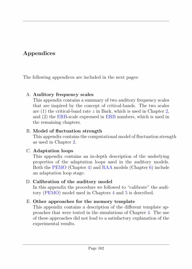
Appendices
The following appendices are included in the next pages:
A. Auditory frequency scalesThis appendix contains a summary of two auditory frequency scalesthat are inspired by the concept of critical-bands. The two scalesare (1) the critical-band rate z in Bark, which is used in Chapter 2,and (2) the ERB-scale expressed in ERB numbers, which is used inthe remaining chapters.
B. Model of fluctuation strengthThis appendix contains the computational model of fluctuation strengthas used in Chapter 2.
C. Adaptation loopsThis appendix contains an in-depth description of the underlyingproperties of the adaptation loops used in the auditory models.Both the PEMO (Chapter 4) and RAA models (Chapter 6) includean adaptation loop stage.
D. Calibration of the auditory modelIn this appendix the procedure we followed to “calibrate” the audi-tory (PEMO) model used in Chapters 4 and 5 is described.
E. Other approaches for the memory templateThis appendix contains a description of the different template ap-proaches that were tested in the simulations of Chapter 4. The useof these approaches did not lead to a satisfactory explanation of theexperimental results.
Page 162
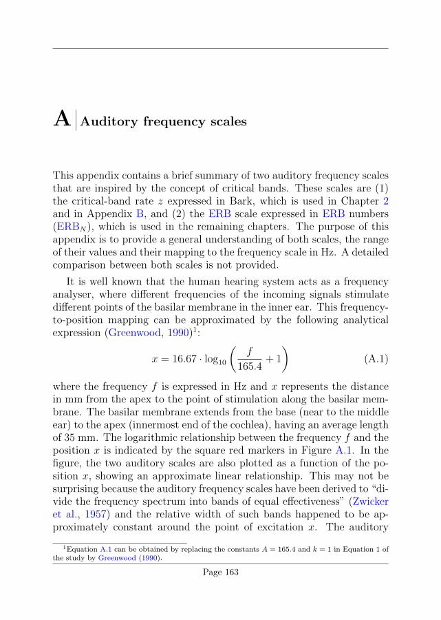
A Auditory frequency scales
This appendix contains a brief summary of two auditory frequency scalesthat are inspired by the concept of critical bands. These scales are (1)the critical-band rate z expressed in Bark, which is used in Chapter 2and in Appendix B, and (2) the ERB scale expressed in ERB numbers(ERBN), which is used in the remaining chapters. The purpose of thisappendix is to provide a general understanding of both scales, the rangeof their values and their mapping to the frequency scale in Hz. A detailedcomparison between both scales is not provided.
It is well known that the human hearing system acts as a frequencyanalyser, where different frequencies of the incoming signals stimulatedifferent points of the basilar membrane in the inner ear. This frequency-to-position mapping can be approximated by the following analyticalexpression (Greenwood, 1990)1:
x = 16.67 · log10
(f
165.4+ 1
)(A.1)
where the frequency f is expressed in Hz and x represents the distancein mm from the apex to the point of stimulation along the basilar mem-brane. The basilar membrane extends from the base (near to the middleear) to the apex (innermost end of the cochlea), having an average lengthof 35 mm. The logarithmic relationship between the frequency f and theposition x is indicated by the square red markers in Figure A.1. In thefigure, the two auditory scales are also plotted as a function of the po-sition x, showing an approximate linear relationship. This may not besurprising because the auditory frequency scales have been derived to “di-vide the frequency spectrum into bands of equal effectiveness” (Zwickeret al., 1957) and the relative width of such bands happened to be ap-proximately constant around the point of excitation x. The auditory
1Equation A.1 can be obtained by replacing the constants A = 165.4 and k = 1 in Equation 1 ofthe study by Greenwood (1990).
Page 163

A Auditory frequency scales
0 4 8 12 16 20 24 28 32 35
0
0.1
0.2
0.3
0.4
0.5
0.6
0.7
0.8
0.9
1
Distance x [mm]
Fre
qu
en
cy s
ca
les [
no
rma
lise
d]
f, Eq. A.1
z, Eq. A.2ERB
N, Eq. A.3
Figure A.1: Frequency-to-position mapping between different frequency scales (normalisedbetween 0 and 1) and the corresponding point of stimulation x along the cochlea. In this fig-ure, the positions x in mm were converted to frequency in Hz (Equation A.1). Subsequentlythe critical-band rate z and the ERBN values were obtained using Equations A.2 and A.3,respectively. Both auditory scales have a nearly linear relationship with the point x.
scales differ, however, in the way they were derived. The critical-bandrate scale z was derived by measuring the width of the “effective bands”in a number of experiments including detection thresholds with complextones and narrow-band noises, amplitude and frequency modulation de-tection, localisation performance and loudness summation (Zwicker etal., 1957; Fastl & Zwicker, 2007, their Chapter 6). The ERB scale mea-sures that bandwidth using a tone-in-notched-noise experiment (see, e.g.,Patterson, 1976).
Both auditory scales are described next by providing an analyticalexpression that maps f onto the corresponding auditory scale. Thisappendix ends by providing a list of tabulated frequencies in Hz andtheir corresponding auditory frequencies z in Bark and in ERBN .
A.1 Critical-band rateAn analytical expression to relate the frequencies z in Bark and f in Hzis given by Equation A.2 (Zwicker & Terhardt, 1980):
z = 13 · arctan(0.76 · 10−4f
)+ 3.5 · arctan
([f
7500
]2)
(A.2)
This expression provides a close mapping between f in Hz and thecritical-band rates z reported by Zwicker (1961). The bandwidth of eachcritical-band is 1 Bark. This leads to about 24 bands in the audiblefrequency range. The reader is referred to Zwicker et al. (1957) andZwicker (1961) for further details about the critical-band rate scale.
Page 164
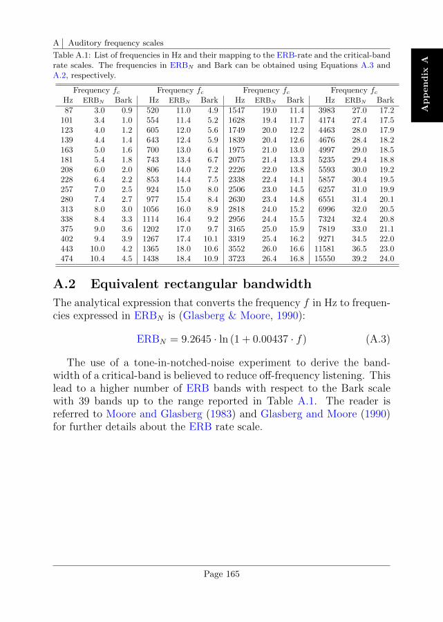
A Auditory frequency scales
Ap
pen
dix
A
Table A.1: List of frequencies in Hz and their mapping to the ERB-rate and the critical-bandrate scales. The frequencies in ERBN and Bark can be obtained using Equations A.3 andA.2, respectively.
Frequency fc Frequency fc Frequency fc Frequency fcHz ERBN Bark Hz ERBN Bark Hz ERBN Bark Hz ERBN Bark87 3.0 0.9 520 11.0 4.9 1547 19.0 11.4 3983 27.0 17.2
101 3.4 1.0 554 11.4 5.2 1628 19.4 11.7 4174 27.4 17.5123 4.0 1.2 605 12.0 5.6 1749 20.0 12.2 4463 28.0 17.9139 4.4 1.4 643 12.4 5.9 1839 20.4 12.6 4676 28.4 18.2163 5.0 1.6 700 13.0 6.4 1975 21.0 13.0 4997 29.0 18.5181 5.4 1.8 743 13.4 6.7 2075 21.4 13.3 5235 29.4 18.8208 6.0 2.0 806 14.0 7.2 2226 22.0 13.8 5593 30.0 19.2228 6.4 2.2 853 14.4 7.5 2338 22.4 14.1 5857 30.4 19.5257 7.0 2.5 924 15.0 8.0 2506 23.0 14.5 6257 31.0 19.9280 7.4 2.7 977 15.4 8.4 2630 23.4 14.8 6551 31.4 20.1313 8.0 3.0 1056 16.0 8.9 2818 24.0 15.2 6996 32.0 20.5338 8.4 3.3 1114 16.4 9.2 2956 24.4 15.5 7324 32.4 20.8375 9.0 3.6 1202 17.0 9.7 3165 25.0 15.9 7819 33.0 21.1402 9.4 3.9 1267 17.4 10.1 3319 25.4 16.2 9271 34.5 22.0443 10.0 4.2 1365 18.0 10.6 3552 26.0 16.6 11581 36.5 23.0474 10.4 4.5 1438 18.4 10.9 3723 26.4 16.8 15550 39.2 24.0
A.2 Equivalent rectangular bandwidth
The analytical expression that converts the frequency f in Hz to frequen-cies expressed in ERBN is (Glasberg & Moore, 1990):
ERBN = 9.2645 · ln (1 + 0.00437 · f) (A.3)
The use of a tone-in-notched-noise experiment to derive the band-width of a critical-band is believed to reduce off-frequency listening. Thislead to a higher number of ERB bands with respect to the Bark scalewith 39 bands up to the range reported in Table A.1. The reader isreferred to Moore and Glasberg (1983) and Glasberg and Moore (1990)for further details about the ERB rate scale.
Page 165

B Modelling the sensation of fluctuation strength1
The sensation of fluctuation strength (FS) is elicited by slow modulationsof a sound, either in amplitude or frequency (typically < 20 Hz), and isrelated to the perception of rhythm. In speech, such periodicities conveyvaluable information for intelligibility (prosody). In western music, mostof the envelope periodicities are also found in that range. These areevidences of the potential relevance of FS in the perception of speech andmusic. In this appendix we present a model of fluctuation strength. Ourmodel was developed taking advantage of the physical similarity betweenFS and the sensation of roughness. The FS model was then adjustedand fitted to existing experimental data collected using artificial stimuli,namely, amplitude- (AM) and frequency- (FM) modulated tones andAM broadband noise (BBN). The test battery of sounds also consists ofsamples of male and female speech and some musical instrument sounds.This FS model has been used in Chapter 2 of this thesis.
B.1 IntroductionTemporal fluctuations in amplitude and in frequency are found natu-rally in everyday sounds. Amplitude modulations (AM) are related tothe envelope of a waveform, while frequency modulations (FM) to itsfine structure. Envelope refers to the perceived acoustic amplitude ofa sound that is integrated by the hearing system due to its slow re-sponse (or “sluggishness”) to high rate (sound pressure) variations ofits waveform. Two examples of everyday sounds are speech and music.Speech was described by Rosen (1992) as temporal fluctuating patternswith three partitions: envelope, periodicity and fine structure. The enve-lope contributes to, among other factors, prosody (i.e., duration, speech
1This chapter is based on:R. Garcıa. (2015)“Modelling the sensation of fluctuation strength”. M.Sc. thesis, Eindhoven Uni-versity of Technology.A. Osses, R. Garcıa, and A. Kohlrausch (2016). “Modelling the sensation of fluctuation strength”.Proc. Mtgs. Acoust., 28(50005), pp. 1–8.
Page 167
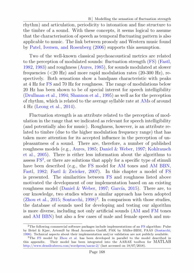
B Modelling the sensation of fluctuation strength
rhythm) and articulation, periodicity to intonation and fine structure tothe timbre of a sound. With these concepts, it seems logical to assumethat the characterisation of speech as temporal fluctuating pattern is alsoapplicable to music. The link between prosody and Western music foundby Patel, Iversen, and Rosenberg (2006) supports this assumption.
Two of the well-known classical psychoacoustical metrics are relatedto the perception of modulated sounds: fluctuation strength (FS) (Fastl,1982, 1983) and roughness (Aures, 1985), for sounds modulated at slowerfrequencies (<20 Hz) and more rapid modulation rates (20-300 Hz), re-spectively. Both sensations show a bandpass characteristic with peaksat 4 Hz for FS and 70 Hz for roughness. The range of modulations below20 Hz has been shown to be of special interest for speech intelligibility(Drullman et al., 1994; Shannon et al., 1995) as well as for the perceptionof rhythm, which is related to the average syllable rate at AMs of around4 Hz (Leong et al., 2014).
Fluctuation strength is an attribute related to the perception of mod-ulation in the range that we indicated as relevant for speech intelligibility(and potentially also for music). Roughness, however, is an attribute re-lated to timbre (due to the higher modulation frequency range) that hastaken more attention for its accepted influence in the perception of un-pleasantness of a sound. There are, therefore, a number of publishedroughness models (e.g., Aures, 1985; Daniel & Weber, 1997; Kohlrauschet al., 2005). There is either less information about the algorithms toassess FS2, or there are solutions that apply for a specific type of stimulihave been described (e.g., the FS model for AM tones and AM BBN,Fastl, 1982; Fastl & Zwicker, 2007). In this chapter a model of FSis presented. The similarities between FS and roughness listed abovemotivated the development of our implementation based on an existingroughness model (Daniel & Weber, 1997; Garcıa, 2015). There are, toour knowledge, two studies where a similar approach has been adopted(Zhou et al., 2015; Sontacchi, 1998)3. In comparison with those studies,the database of sounds used for developing and testing our algorithmis more diverse, including not only artificial sounds (AM and FM tonesand AM BBN) but also a few cases of male and female speech and mu-
2The following commercial software packages include implementations of an FS algorithm: Pulseby Bruel & Kjær, ArtemiS by Head Acoustics GmbH, PAK by Muller-BBM, PAAS (Sontacchi,1998). Technical aspects about their implementation and/or validation are not publicly available.
3The FS model by Zhou et al. has been developed in parallel to the model described inthis appendix. Their model has been integrated into the AARAE toolbox for MATLABhttp://www.densilcabrera.com/wordpress/aarae-2/ (last accessed on 18/07/2018).
Page 168
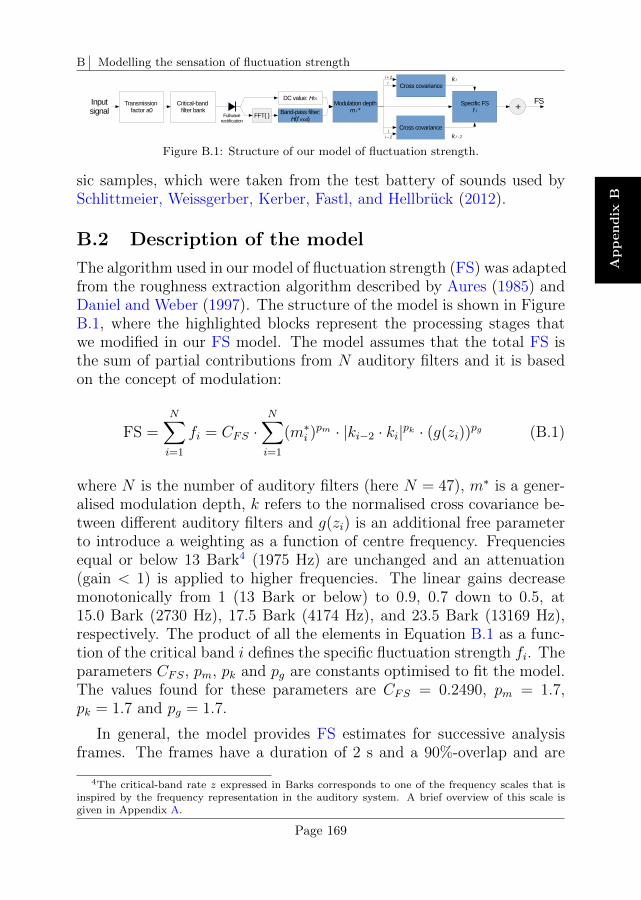
B Modelling the sensation of fluctuation strength
Ap
pen
dix
B
Figure B.1: Structure of our model of fluctuation strength.
sic samples, which were taken from the test battery of sounds used bySchlittmeier, Weissgerber, Kerber, Fastl, and Hellbruck (2012).
B.2 Description of the model
The algorithm used in our model of fluctuation strength (FS) was adaptedfrom the roughness extraction algorithm described by Aures (1985) andDaniel and Weber (1997). The structure of the model is shown in FigureB.1, where the highlighted blocks represent the processing stages thatwe modified in our FS model. The model assumes that the total FS isthe sum of partial contributions from N auditory filters and it is basedon the concept of modulation:
FS =N∑i=1
fi = CFS ·N∑i=1
(m∗i )pm · |ki−2 · ki|pk · (g(zi))
pg (B.1)
where N is the number of auditory filters (here N = 47), m∗ is a gener-alised modulation depth, k refers to the normalised cross covariance be-tween different auditory filters and g(zi) is an additional free parameterto introduce a weighting as a function of centre frequency. Frequenciesequal or below 13 Bark4 (1975 Hz) are unchanged and an attenuation(gain < 1) is applied to higher frequencies. The linear gains decreasemonotonically from 1 (13 Bark or below) to 0.9, 0.7 down to 0.5, at15.0 Bark (2730 Hz), 17.5 Bark (4174 Hz), and 23.5 Bark (13169 Hz),respectively. The product of all the elements in Equation B.1 as a func-tion of the critical band i defines the specific fluctuation strength fi. Theparameters CFS, pm, pk and pg are constants optimised to fit the model.The values found for these parameters are CFS = 0.2490, pm = 1.7,pk = 1.7 and pg = 1.7.
In general, the model provides FS estimates for successive analysisframes. The frames have a duration of 2 s and a 90%-overlap and are
4The critical-band rate z expressed in Barks corresponds to one of the frequency scales that isinspired by the frequency representation in the auditory system. A brief overview of this scale isgiven in Appendix A.
Page 169
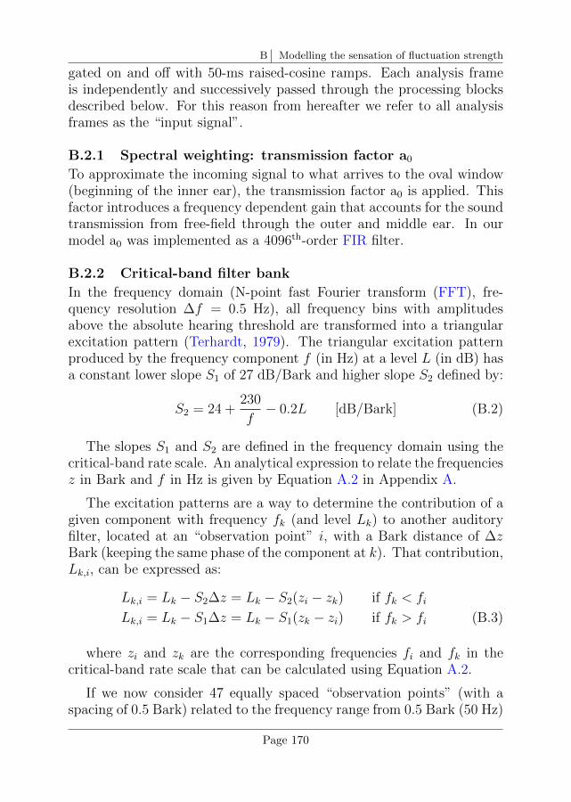
B Modelling the sensation of fluctuation strength
gated on and off with 50-ms raised-cosine ramps. Each analysis frameis independently and successively passed through the processing blocksdescribed below. For this reason from hereafter we refer to all analysisframes as the “input signal”.
B.2.1 Spectral weighting: transmission factor a0
To approximate the incoming signal to what arrives to the oval window(beginning of the inner ear), the transmission factor a0 is applied. Thisfactor introduces a frequency dependent gain that accounts for the soundtransmission from free-field through the outer and middle ear. In ourmodel a0 was implemented as a 4096th-order FIR filter.
B.2.2 Critical-band filter bank
In the frequency domain (N-point fast Fourier transform (FFT), fre-quency resolution ∆f = 0.5 Hz), all frequency bins with amplitudesabove the absolute hearing threshold are transformed into a triangularexcitation pattern (Terhardt, 1979). The triangular excitation patternproduced by the frequency component f (in Hz) at a level L (in dB) hasa constant lower slope S1 of 27 dB/Bark and higher slope S2 defined by:
S2 = 24 +230
f− 0.2L [dB/Bark] (B.2)
The slopes S1 and S2 are defined in the frequency domain using thecritical-band rate scale. An analytical expression to relate the frequenciesz in Bark and f in Hz is given by Equation A.2 in Appendix A.
The excitation patterns are a way to determine the contribution of agiven component with frequency fk (and level Lk) to another auditoryfilter, located at an “observation point” i, with a Bark distance of ∆zBark (keeping the same phase of the component at k). That contribution,Lk,i, can be expressed as:
Lk,i = Lk − S2∆z = Lk − S2(zi − zk) if fk < fi
Lk,i = Lk − S1∆z = Lk − S1(zk − zi) if fk > fi (B.3)
where zi and zk are the corresponding frequencies fi and fk in thecritical-band rate scale that can be calculated using Equation A.2.
If we now consider 47 equally spaced “observation points” (with aspacing of 0.5 Bark) related to the frequency range from 0.5 Bark (50 Hz)
Page 170
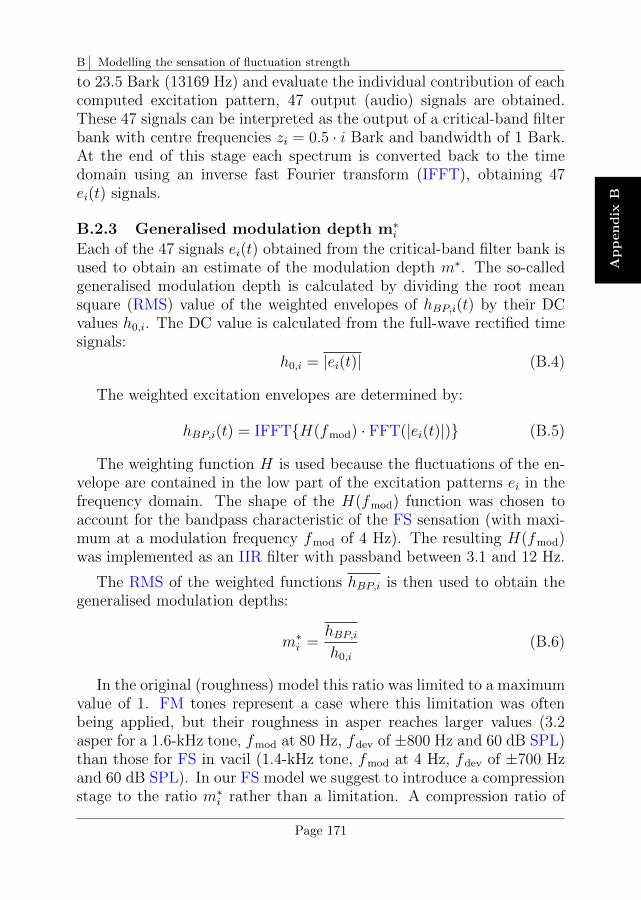
B Modelling the sensation of fluctuation strength
Ap
pen
dix
B
to 23.5 Bark (13169 Hz) and evaluate the individual contribution of eachcomputed excitation pattern, 47 output (audio) signals are obtained.These 47 signals can be interpreted as the output of a critical-band filterbank with centre frequencies zi = 0.5 · i Bark and bandwidth of 1 Bark.At the end of this stage each spectrum is converted back to the timedomain using an inverse fast Fourier transform (IFFT), obtaining 47ei(t) signals.
B.2.3 Generalised modulation depth m∗iEach of the 47 signals ei(t) obtained from the critical-band filter bank isused to obtain an estimate of the modulation depth m∗. The so-calledgeneralised modulation depth is calculated by dividing the root meansquare (RMS) value of the weighted envelopes of hBP,i(t) by their DCvalues h0,i. The DC value is calculated from the full-wave rectified timesignals:
h0,i = |ei(t)| (B.4)
The weighted excitation envelopes are determined by:
hBP,i(t) = IFFTH(fmod) · FFT(|ei(t)|) (B.5)
The weighting function H is used because the fluctuations of the en-velope are contained in the low part of the excitation patterns ei in thefrequency domain. The shape of the H(fmod) function was chosen toaccount for the bandpass characteristic of the FS sensation (with maxi-mum at a modulation frequency fmod of 4 Hz). The resulting H(fmod)was implemented as an IIR filter with passband between 3.1 and 12 Hz.
The RMS of the weighted functions hBP,i is then used to obtain thegeneralised modulation depths:
m∗i =hBP,ih0,i
(B.6)
In the original (roughness) model this ratio was limited to a maximumvalue of 1. FM tones represent a case where this limitation was oftenbeing applied, but their roughness in asper reaches larger values (3.2asper for a 1.6-kHz tone, fmod at 80 Hz, fdev of ±800 Hz and 60 dB SPL)than those for FS in vacil (1.4-kHz tone, fmod at 4 Hz, fdev of ±700 Hzand 60 dB SPL). In our FS model we suggest to introduce a compressionstage to the ratio m∗i rather than a limitation. A compression ratio of
Page 171

B Modelling the sensation of fluctuation strength
3:1 is applied when the modulation depth estimate exceeds a thresholdof 0.7 units. This means that if m∗i is 0.15 units above the threshold,i.e., m∗i input = 0.85 the resulting modulation depth will be 0.05 (0.15/3)above threshold resulting in m∗i output = 0.75.
B.2.4 Normalised cross covariance
In a discrete time domain the normalised cross covariance (in short, crosscovariance) between the functions x and y, both being N samples long,is defined by Equation B.7 (see, e.g., van de Par & Kohlrausch, 1995,their Equation 2):
k =
∑xy − 1
N
∑x∑y√[∑
x2 − 1N
(∑x)2] [∑
y2 − 1N
(∑y)2] (B.7)
Within our computational model the cross covariance between adja-cent critical bands is assessed to determine whether their modulationsare in or out of phase. The more in-phase the modulations are deter-mines to what extent the specific FS can be summed up to obtain thetotal FS. In this manner, the cross covariance between the channel i andthe channels one Bark below i − 2 and above i + 2 are computed. Inother words, to obtain the factor ki−2, x and y in Equation B.7 have tobe replaced by hBP,i−2 and hBP,i, respectively. Likewise, to obtain thefactor ki, x and y have to be replaced by hBP,i and hBP,i+2.
B.3 Validation of the model
In order to fit and validate the FS model presented in this appendix, a setof stimuli with known values were chosen. Part of the set correspondedto artificial stimuli: AM tones, FM tones, and AM BBN. The rest ofthe stimuli were chosen from a set of everyday sounds. The referencesound to which an FS of 1 vacil is ascribed is an AM sine tone centredat fc = 1000 Hz, modulated at an fmod of 4 Hz and level of 60 dB.A summary of the artificial stimuli used in the validation is shown inTable B.1. For this set of stimuli, FS values obtained in perceptualexperiments are available (Fastl & Zwicker, 2007, their Chapter 11).Additionally, a set of everyday sounds were extracted from the databaseof sounds used by Schlittmeier et al. (2012). That database consists of70 sounds, out of which 7 representative sound samples were chosen.The selection of the samples was as follows: (a) three representativespeech samples (one male voice, one female voice, babble noise); (b)
Page 172
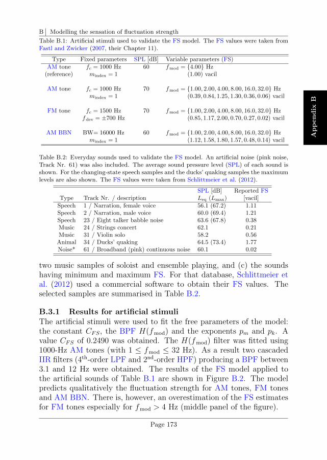
B Modelling the sensation of fluctuation strength
Ap
pen
dix
B
Table B.1: Artificial stimuli used to validate the FS model. The FS values were taken fromFastl and Zwicker (2007, their Chapter 11).
Type Fixed parameters SPL [dB] Variable parameters (FS)AM tone fc = 1000 Hz 60 fmod = 4.00 Hz
(reference) mindex = 1 (1.00) vacil
AM tone fc = 1000 Hz 70 fmod = 1.00, 2.00, 4.00, 8.00, 16.0, 32.0 Hzmindex = 1 (0.39, 0.84, 1.25, 1.30, 0.36, 0.06) vacil
FM tone fc = 1500 Hz 70 fmod = 1.00, 2.00, 4.00, 8.00, 16.0, 32.0 Hzfdev = ±700 Hz (0.85, 1.17, 2.00, 0.70, 0.27, 0.02) vacil
AM BBN BW= 16000 Hz 60 fmod = 1.00, 2.00, 4.00, 8.00, 16.0, 32.0 Hzmindex = 1 (1.12, 1.58, 1.80, 1.57, 0.48, 0.14) vacil
Table B.2: Everyday sounds used to validate the FS model. An artificial noise (pink noise,Track Nr. 61) was also included. The average sound pressure level (SPL) of each sound isshown. For the changing-state speech samples and the ducks’ quaking samples the maximumlevels are also shown. The FS values were taken from Schlittmeier et al. (2012).
SPL [dB] Reported FSType Track Nr. / description Leq (Lmax) [vacil]
Speech 1 / Narration, female voice 56.1 (67.2) 1.11Speech 2 / Narration, male voice 60.0 (69.4) 1.21Speech 23 / Eight talker babble noise 63.6 (67.8) 0.38Music 24 / Strings concert 62.1 0.21Music 31 / Violin solo 58.2 0.56
Animal 34 / Ducks’ quaking 64.5 (73.4) 1.77Noise* 61 / Broadband (pink) continuous noise 60.1 0.02
two music samples of soloist and ensemble playing, and (c) the soundshaving minimum and maximum FS. For that database, Schlittmeier etal. (2012) used a commercial software to obtain their FS values. Theselected samples are summarised in Table B.2.
B.3.1 Results for artificial stimuliThe artificial stimuli were used to fit the free parameters of the model:the constant CFS, the BPF H(fmod) and the exponents pm and pk. Avalue CFS of 0.2490 was obtained. The H(fmod) filter was fitted using1000-Hz AM tones (with 1 ≤ fmod ≤ 32 Hz). As a result two cascadedIIR filters (4th-order LPF and 2nd-order HPF) producing a BPF between3.1 and 12 Hz were obtained. The results of the FS model applied tothe artificial sounds of Table B.1 are shown in Figure B.2. The modelpredicts qualitatively the fluctuation strength for AM tones, FM tonesand AM BBN. There is, however, an overestimation of the FS estimatesfor FM tones especially for fmod > 4 Hz (middle panel of the figure).
Page 173
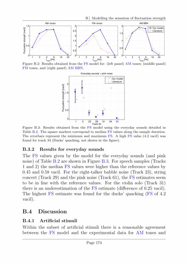
B Modelling the sensation of fluctuation strength
1 2 4 8 16 320
0.5
1
1.5
fmod
[Hz]
Flu
ctu
ation s
trength
[vacil]
AM−tones
1 2 4 8 16 320
0.5
1
1.5
2
2.5
3
fmod
[Hz]
Flu
ctu
ation s
trength
[vacil]
FM−tones
1 2 4 8 16 320
0.5
1
1.5
2
fmod
[Hz]
Flu
ctu
ation s
trength
[vacil]
AM BBN
Our model
Literature
Figure B.2: Results obtained from the FS model for: (left panel) AM tones; (middle panel)FM tones, and (right panel) AM BBN.
1 2 23 29 31 34 610
0.5
1
1.5
2
Track Nr.
Flu
ctu
ation s
trength
[vacil]
Everyday sounds + pink noise
Our model
Literature
Figure B.3: Results obtained from the FS model using the everyday sounds detailed inTable B.2. The square markers correspond to median FS values along the sample duration.The errorbars represent the minimum and maximum FS. A high FS value (4.2 vacil) wasfound for track 34 (Ducks’ quacking, not shown in the figure).
B.3.2 Results for everyday sounds
The FS values given by the model for the everyday sounds (and pinknoise) of Table B.2 are shown in Figure B.3. For speech samples (Tracks1 and 2) the median FS values were higher than the reference values by0.45 and 0.58 vacil. For the eight-talker babble noise (Track 23), stringconcert (Track 29) and the pink noise (Track 61), the FS estimates seemto be in line with the reference values. For the violin solo (Track 31)there is an underestimation of the FS estimate (difference of 0.25 vacil).The highest FS estimate was found for the ducks’ quacking (FS of 4.2vacil).
B.4 Discussion
B.4.1 Artificial stimuli
Within the subset of artificial stimuli there is a reasonable agreementbetween the FS model and the experimental data for AM tones and
Page 174
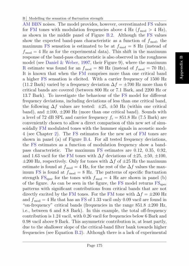
B Modelling the sensation of fluctuation strength
Ap
pen
dix
B
AM BBN noises. The model provides, however, overestimated FS valuesfor FM tones with modulation frequencies above 4 Hz (fmod > 4 Hz),as shown in the middle panel of Figure B.2. Although the FS valuesshow the expected band-pass characteristic as a function of fmod, themaximum FS sensation is estimated to be at fmod = 8 Hz (instead offmod = 4 Hz as for the experimental data). This shift in the maximumresponse of the band-pass characteristic is also observed in the roughnessmodel (see Daniel & Weber, 1997, their Figure 9), where the maximumR estimate was found for an fmod = 80 Hz (instead of fmod = 70 Hz).It is known that when the FM comprises more than one critical banda higher FS sensation is elicited. With a carrier frequency of 1500 Hz(11.2 Bark) varied by a frequency deviation ∆f = ±700 Hz more than 6critical bands are covered (between 800 Hz or 7.1 Bark, and 2200 Hz or13.7 Bark). To investigate the behaviour of the FS model for differentfrequency deviations, including deviations of less than one critical band,the following ∆f values are tested: ±25, ±50 Hz (within one criticalband), and ±100, ±200 Hz (more than one critical band). Sounds witha level of 72 dB SPL and carrier frequency fc = 851.8 Hz (7.5 Bark) areconveniently chosen to allow a direct comparison of this new set of sinu-soidally FM modulated tones with the hummer signals in acoustic mode4 (see Chapter 2). The FS estimates for the new set of FM tones areshown in panel (a) of Figure B.4. For all tested frequency deviations,the FS estimates as a function of modulation frequency show a band-pass characteristic. The maximum FS estimates are 0.12, 0.35, 0.92,and 1.63 vacil for the FM tones with ∆f deviations of ±25, ±50, ±100,±200 Hz, respectively. Only for tones with ∆f of ±25 Hz the maximumestimate is found at fmod = 4 Hz, for the rest of the ∆f values the max-imum FS is found at fmod = 8 Hz. The patterns of specific fluctuationstrength FSspec for the tones with fmod = 4 Hz are shown in panel (b)of the figure. As can be seen in the figure, the FS model returns FSspec
patterns with significant contributions from critical bands that are notdirectly excited by the FM tones. For the FM tone with ∆f = ±200 Hzand fmod = 4 Hz that has an FS of 1.33 vacil only 0.09 vacil are found in“on-frequency” critical bands (frequencies in the range 851.8 ±200 Hz,i.e., between 6 and 8.8 Bark). In this example, the total off-frequencycontribution is 1.24 vacil, with 0.26 vacil for frequencies below 6 Bark and0.98 vacil above 9 Bark. This asymmetric contribution is, at least partly,due to the shallower slope of the critical-band filter bank towards higherfrequencies (see Equation B.2). Although there is a lack of experimental
Page 175

B Modelling the sensation of fluctuation strength
1 2 4 8 16 32
0.10.20.30.40.50.60.70.80.9
11.11.21.31.41.51.6
fmod
[Hz]
Flu
ctu
atio
n s
tre
ng
th [
va
cil]
(a)
∆ f=± 25 Hz
∆ f=± 50 Hz
∆ f=± 100 Hz
∆ f=± 200 Hz
4.5 5.5 6.5 7.5 8.5 9.5 10.5 11.5 12.5 13.5−0.1
−0.05
0
0.05
0.1
0.15
0.2
0.25
0.3
0.35
0.4
Critical−band rate [Bark]
Sp
ecific
fi [
va
cil/
Ba
rk]
(b)
Figure B.4: (a) Fluctuation strength FS values and (b) specific fluctuation strength patternsFSspec (only for tones with fmod = 4 Hz) for sinusoidally FM tones centred at 851.8 Hz witha level of 72 dB SPL that are modulated using frequency deviations ∆f of ±25, ±50, ±100,±200 Hz. For this carrier frequency, the first two ∆f values produce oscillations in frequencywithin one critical band (between 7 and 8 Bark). The FM tone with ∆f of ±200 Hz coversthe frequency range between 651.8 Hz (6 Bark) and 1051.8 Hz (8.8 Bark).
evidence for the FS estimates shown in panel (a) of Figure B.4, the band-pass characteristic built from experimental FS data collected by Garcıafrom 20 participants for 70-dB FM tones, fc = 1500 Hz, ∆f = ±700 Hz,and 0 ≤ fmod ≤ 128 Hz (similar stimuli as used in panel (b) of Fig-ure B.2) had its maximum FS value at fmod = 8 Hz (Garcıa, 2015, hisFigure 5.5(b)).
B.4.2 Everyday soundsWithin the set of everyday sounds there is a good approximation betweenFS values and the estimates in the reference paper for the eight-talkerbabble noise, the string concert and the pink noise samples. Higher FSvalues for the male and female voices and the ducks’ quacking soundsand a lower value for the violin sample. For the male, female and ducks’quacking sounds our model provides high modulation depth m∗ values,with a median across bands of 0.81, 0.95, and 0.86, respectively. Themedian cross covariance k for the same samples are 0.50, 0.20, and 0.83.It is noteworthy that the modulation depth m∗ values in our model areassessed with respect to the DC values h0, independent of the level ofh0. This means that the higher FS estimates in our model may be aconsequence of the high m∗ values. However, it is also important to pointout that the estimates presented in the reference paper were obtainedfrom another FS algorithm and, therefore, it is unclear whether thoseFS values have been validated experimentally.
Page 176
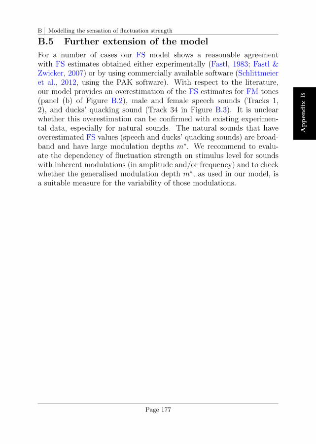
B Modelling the sensation of fluctuation strength
Ap
pen
dix
B
B.5 Further extension of the model
For a number of cases our FS model shows a reasonable agreementwith FS estimates obtained either experimentally (Fastl, 1983; Fastl &Zwicker, 2007) or by using commercially available software (Schlittmeieret al., 2012, using the PAK software). With respect to the literature,our model provides an overestimation of the FS estimates for FM tones(panel (b) of Figure B.2), male and female speech sounds (Tracks 1,2), and ducks’ quacking sound (Track 34 in Figure B.3). It is unclearwhether this overestimation can be confirmed with existing experimen-tal data, especially for natural sounds. The natural sounds that haveoverestimated FS values (speech and ducks’ quacking sounds) are broad-band and have large modulation depths m∗. We recommend to evalu-ate the dependency of fluctuation strength on stimulus level for soundswith inherent modulations (in amplitude and/or frequency) and to checkwhether the generalised modulation depth m∗, as used in our model, isa suitable measure for the variability of those modulations.
Page 177

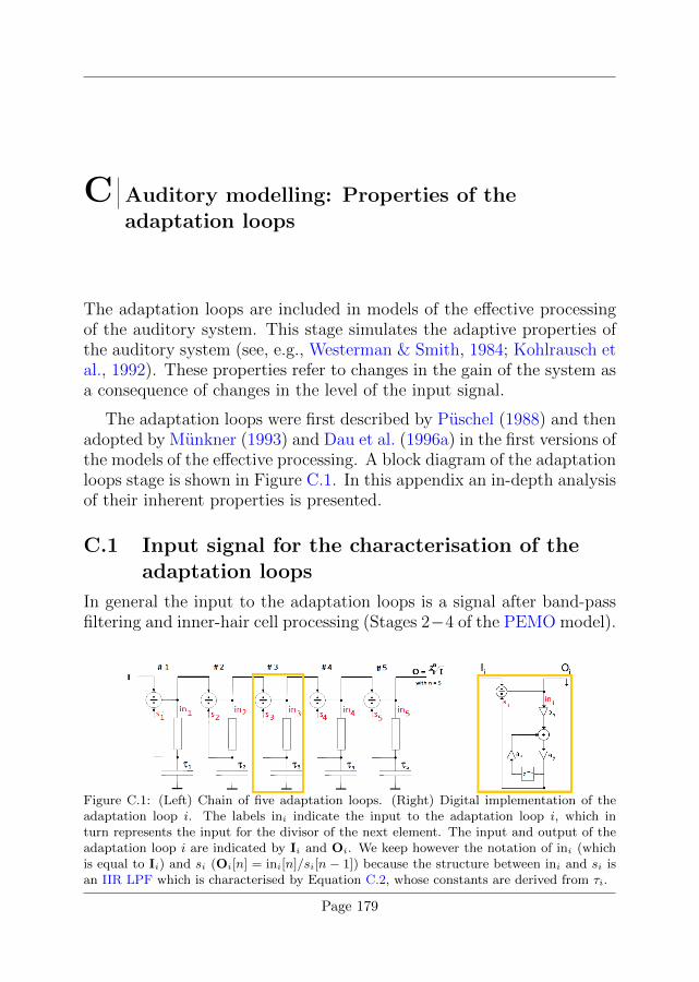
C Auditory modelling: Properties of theadaptation loops
The adaptation loops are included in models of the effective processingof the auditory system. This stage simulates the adaptive properties ofthe auditory system (see, e.g., Westerman & Smith, 1984; Kohlrausch etal., 1992). These properties refer to changes in the gain of the system asa consequence of changes in the level of the input signal.
The adaptation loops were first described by Puschel (1988) and thenadopted by Munkner (1993) and Dau et al. (1996a) in the first versions ofthe models of the effective processing. A block diagram of the adaptationloops stage is shown in Figure C.1. In this appendix an in-depth analysisof their inherent properties is presented.
C.1 Input signal for the characterisation of theadaptation loops
In general the input to the adaptation loops is a signal after band-passfiltering and inner-hair cell processing (Stages 2−4 of the PEMO model).
Figure C.1: (Left) Chain of five adaptation loops. (Right) Digital implementation of theadaptation loop i. The labels ini indicate the input to the adaptation loop i, which inturn represents the input for the divisor of the next element. The input and output of theadaptation loop i are indicated by Ii and Oi. We keep however the notation of ini (whichis equal to Ii) and si (Oi[n] = ini[n]/si[n− 1]) because the structure between ini and si isan IIR LPF which is characterised by Equation C.2, whose constants are derived from τi.
Page 179

C Auditory modelling: Properties of the adaptation loops
50 150 250 350 450 550 650 750
0
0.1
0.2
0.3
0.4
0.5
0.6
0.7
0.8
0.9
1
Time [ms]
Am
plitu
de
Pulse signal after ihc−breebaart
40 42 44 46 48 50 52 54 56 58 60
0
0.1
0.2
0.3
0.4
0.5
0.6
0.7
0.8
0.9
1
Time [ms]
Am
plitu
de
Pulse signal after ihc−breebaart (zoomed)
Figure C.2: Steady-state signal used to generate the analyses presented in this section. Thesignal has unit amplitude, duration of 300 ms with the signal onset at 50 ms and it includesan up-down cosine ramp of 1 ms. The cosine ramp introduces a similar effect to the pulseas the inner-hair cell stage of the PEMO model would do. The right panel corresponds tothe same pulse as in the left panel but zoomed in to appreciate the raised cosine ramp.
In the analyses of this appendix we only account for the inner-hair cellprocessing. Therefore, the input x[n] corresponds to a digital waveformafter half-wave rectification and a low-pass filtering with a cut-off fre-quency of 770 Hz. The input x[n] is scaled between 0 and 1.
The analyses presented in the subsequent subsections (C.2 and C.3)are generated using the pulse signal that is shown in Figure C.2. Thepulse signal has unit amplitude (steady-state input of 100 dB SPL),a duration of 300 ms and it is preceded and succeeded by 50 ms and450 ms of silence, resulting in a signal 800 ms long. To facilitate thereproducibility of the analyses, the pulse was ramped up and down witha cosine ramp of 1 ms. The cosine ramp introduces a similar effect tothe pulse signal as the stage of inner hair-cell processing of the PEMOmodel would do (Stages 3 and 4 in the diagram of Figure 4.1, page 56)1.
C.2 Adaptation and use of the RC analogy
The adaptation stage comprises a chain of 5 adaptation loops, which isshown in Figure C.1. Each adaptation loop corresponds to a Resistor-Capacitor (RC) circuit that acts as a low-pass filter between the nodeini and the value si, with i = 1, 2, 3, 4, 5. The output si representsthe charging state of the low-pass filter. The low-pass filters are imple-mented as first-order IIR filters and their time constants relate to theircut-off frequencies according to: τi = 1/(2π · f cut-off). The outputs sifor a steady-state input of amplitude 1 are shown in Figure C.3. As
1For this analysis the effect of the Stages 1 (Outer and middle ear filtering) and 2 (ERB filterbank) of the PEMO model were omitted.
Page 180
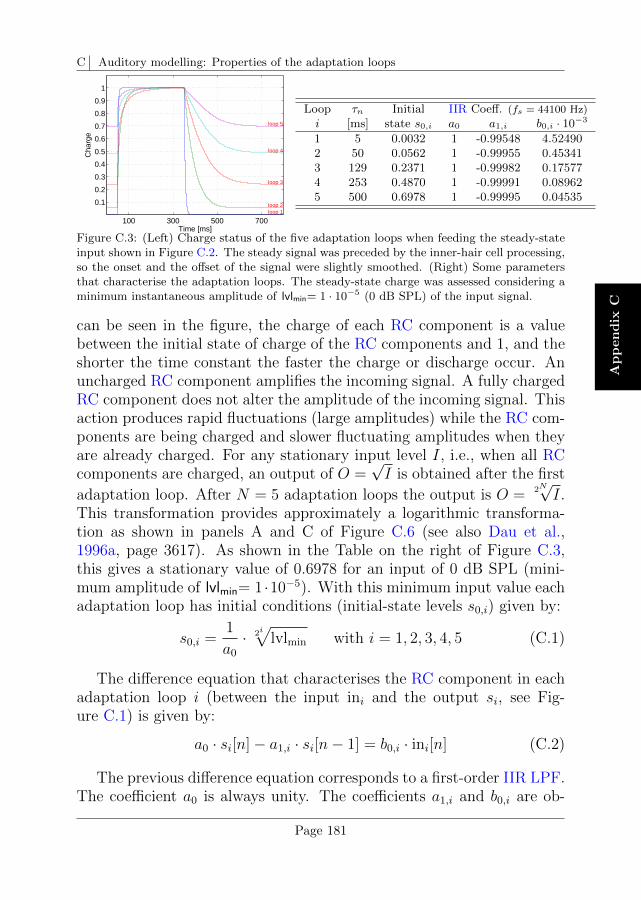
C Auditory modelling: Properties of the adaptation loops
Ap
pen
dix
C
100 300 500 700
0.1
0.2
0.3
0.4
0.5
0.6
0.7
0.8
0.9
1
Time [ms]
Cha
rge
loop 1loop 2
loop 3
loop 4
loop 5
Loop τn Initial IIR Coeff. (fs = 44100 Hz)
i [ms] state s0,i a0 a1,i b0,i · 10−3
1 5 0.0032 1 -0.99548 4.524902 50 0.0562 1 -0.99955 0.453413 129 0.2371 1 -0.99982 0.175774 253 0.4870 1 -0.99991 0.089625 500 0.6978 1 -0.99995 0.04535
Figure C.3: (Left) Charge status of the five adaptation loops when feeding the steady-stateinput shown in Figure C.2. The steady signal was preceded by the inner-hair cell processing,so the onset and the offset of the signal were slightly smoothed. (Right) Some parametersthat characterise the adaptation loops. The steady-state charge was assessed considering aminimum instantaneous amplitude of lvlmin= 1 · 10−5 (0 dB SPL) of the input signal.
can be seen in the figure, the charge of each RC component is a valuebetween the initial state of charge of the RC components and 1, and theshorter the time constant the faster the charge or discharge occur. Anuncharged RC component amplifies the incoming signal. A fully chargedRC component does not alter the amplitude of the incoming signal. Thisaction produces rapid fluctuations (large amplitudes) while the RC com-ponents are being charged and slower fluctuating amplitudes when theyare already charged. For any stationary input level I, i.e., when all RCcomponents are charged, an output of O =
√I is obtained after the first
adaptation loop. After N = 5 adaptation loops the output is O = 2N√I.
This transformation provides approximately a logarithmic transforma-tion as shown in panels A and C of Figure C.6 (see also Dau et al.,1996a, page 3617). As shown in the Table on the right of Figure C.3,this gives a stationary value of 0.6978 for an input of 0 dB SPL (mini-mum amplitude of lvlmin= 1 ·10−5). With this minimum input value eachadaptation loop has initial conditions (initial-state levels s0,i) given by:
s0,i =1
a0
· 2i√
lvlmin with i = 1, 2, 3, 4, 5 (C.1)
The difference equation that characterises the RC component in eachadaptation loop i (between the input ini and the output si, see Fig-ure C.1) is given by:
a0 · si[n]− a1,i · si[n− 1] = b0,i · ini[n] (C.2)
The previous difference equation corresponds to a first-order IIR LPF.The coefficient a0 is always unity. The coefficients a1,i and b0,i are ob-
Page 181
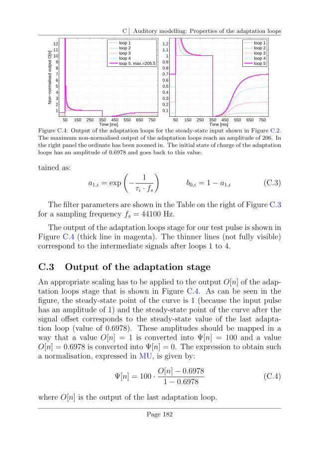
C Auditory modelling: Properties of the adaptation loops
50 150 250 350 450 550 650 750
123456789
101112
Time [ms]
Non
−no
rmal
ised
out
put O
[n]
No overshoot limitation
loop 1loop 2loop 3loop 4loop 5, max.=205.5
50 150 250 350 450 550 650 750
0.10.20.30.40.50.60.70.80.9
11.11.2
Time [ms]
Non
−no
rmal
ised
out
put O
[n]
No overshoot limitation (zoomed)
loop 1loop 2loop 3loop 4loop 5
Figure C.4: Output of the adaptation loops for the steady-state input shown in Figure C.2.The maximum non-normalised output of the adaptation loops reach an amplitude of 206. Inthe right panel the ordinate has been zoomed in. The initial state of charge of the adaptationloops has an amplitude of 0.6978 and goes back to this value.
tained as:
a1,i = exp
(− 1
τi · fs
)b0,i = 1− a1,i (C.3)
The filter parameters are shown in the Table on the right of Figure C.3for a sampling frequency fs = 44100 Hz.
The output of the adaptation loops stage for our test pulse is shown inFigure C.4 (thick line in magenta). The thinner lines (not fully visible)correspond to the intermediate signals after loops 1 to 4.
C.3 Output of the adaptation stage
An appropriate scaling has to be applied to the output O[n] of the adap-tation loops stage that is shown in Figure C.4. As can be seen in thefigure, the steady-state point of the curve is 1 (because the input pulsehas an amplitude of 1) and the steady-state point of the curve after thesignal offset corresponds to the steady-state value of the last adapta-tion loop (value of 0.6978). These amplitudes should be mapped in away that a value O[n] = 1 is converted into Ψ[n] = 100 and a valueO[n] = 0.6978 is converted into Ψ[n] = 0. The expression to obtain sucha normalisation, expressed in MU, is given by:
Ψ[n] = 100 · O[n]− 0.6978
1− 0.6978(C.4)
where O[n] is the output of the last adaptation loop.
Page 182
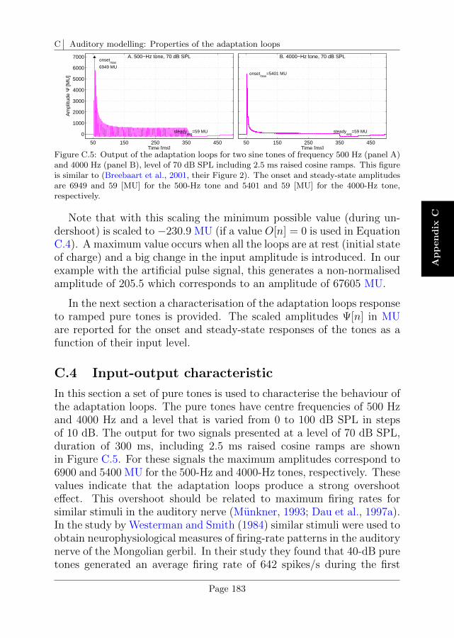
C Auditory modelling: Properties of the adaptation loops
Ap
pen
dix
C
50 150 250 350 450
0
1000
2000
3000
4000
5000
6000
7000
Time [ms]
Am
plitu
de Ψ
[MU
]
A. 500−Hz tone, 70 dB SPL
steadyavg
=59 MU
onsetmax
6949 MU
50 150 250 350 450
0
1000
2000
3000
4000
5000
6000
7000
Time [ms]
Am
plitu
de Ψ
[MU
]
B. 4000−Hz tone, 70 dB SPL
steadyavg
=59 MU
onsetmax
=5401 MU
Figure C.5: Output of the adaptation loops for two sine tones of frequency 500 Hz (panel A)and 4000 Hz (panel B), level of 70 dB SPL including 2.5 ms raised cosine ramps. This figureis similar to (Breebaart et al., 2001, their Figure 2). The onset and steady-state amplitudesare 6949 and 59 [MU] for the 500-Hz tone and 5401 and 59 [MU] for the 4000-Hz tone,respectively.
Note that with this scaling the minimum possible value (during un-dershoot) is scaled to −230.9 MU (if a value O[n] = 0 is used in EquationC.4). A maximum value occurs when all the loops are at rest (initial stateof charge) and a big change in the input amplitude is introduced. In ourexample with the artificial pulse signal, this generates a non-normalisedamplitude of 205.5 which corresponds to an amplitude of 67605 MU.
In the next section a characterisation of the adaptation loops responseto ramped pure tones is provided. The scaled amplitudes Ψ[n] in MUare reported for the onset and steady-state responses of the tones as afunction of their input level.
C.4 Input-output characteristic
In this section a set of pure tones is used to characterise the behaviour ofthe adaptation loops. The pure tones have centre frequencies of 500 Hzand 4000 Hz and a level that is varied from 0 to 100 dB SPL in stepsof 10 dB. The output for two signals presented at a level of 70 dB SPL,duration of 300 ms, including 2.5 ms raised cosine ramps are shownin Figure C.5. For these signals the maximum amplitudes correspond to6900 and 5400 MU for the 500-Hz and 4000-Hz tones, respectively. Thesevalues indicate that the adaptation loops produce a strong overshooteffect. This overshoot should be related to maximum firing rates forsimilar stimuli in the auditory nerve (Munkner, 1993; Dau et al., 1997a).In the study by Westerman and Smith (1984) similar stimuli were used toobtain neurophysiological measures of firing-rate patterns in the auditorynerve of the Mongolian gerbil. In their study they found that 40-dB puretones generated an average firing rate of 642 spikes/s during the first
Page 183
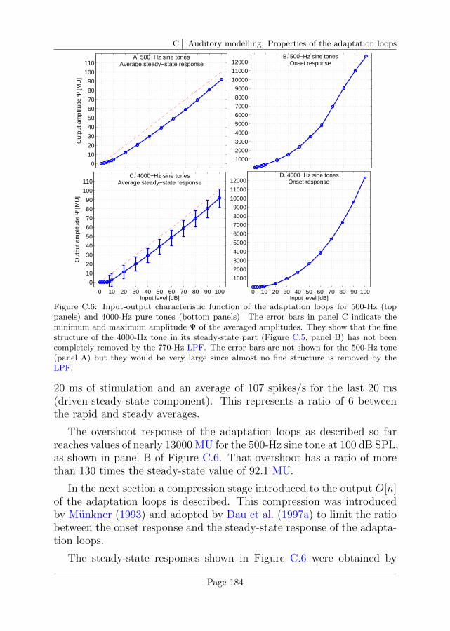
C Auditory modelling: Properties of the adaptation loops
0 10 20 30 40 50 60 70 80 90 100
0
10
20
30
40
50
60
70
80
90
100
110
Input level [dB]
Out
put a
mpl
itude
Ψ [M
U]
A. 500−Hz sine tonesAverage steady−state response
0 10 20 30 40 50 60 70 80 90 100
1000
2000
3000
4000
5000
6000
7000
8000
9000
10000
11000
12000
Input level [dB]
Out
put a
mpl
itude
Ψ [M
U]
B. 500−Hz sine tonesOnset response
0 10 20 30 40 50 60 70 80 90 100
0
10
20
30
40
50
60
70
80
90
100
110
Input level [dB]
Out
put a
mpl
itude
Ψ [M
U]
C. 4000−Hz sine tonesAverage steady−state response
0 10 20 30 40 50 60 70 80 90 100
1000
2000
3000
4000
5000
6000
7000
8000
9000
10000
11000
12000
Input level [dB]
Out
put a
mpl
itude
Ψ [M
U]
D. 4000−Hz sine tonesOnset response
Figure C.6: Input-output characteristic function of the adaptation loops for 500-Hz (toppanels) and 4000-Hz pure tones (bottom panels). The error bars in panel C indicate theminimum and maximum amplitude Ψ of the averaged amplitudes. They show that the finestructure of the 4000-Hz tone in its steady-state part (Figure C.5, panel B) has not beencompletely removed by the 770-Hz LPF. The error bars are not shown for the 500-Hz tone(panel A) but they would be very large since almost no fine structure is removed by theLPF.
20 ms of stimulation and an average of 107 spikes/s for the last 20 ms(driven-steady-state component). This represents a ratio of 6 betweenthe rapid and steady averages.
The overshoot response of the adaptation loops as described so farreaches values of nearly 13000 MU for the 500-Hz sine tone at 100 dB SPL,as shown in panel B of Figure C.6. That overshoot has a ratio of morethan 130 times the steady-state value of 92.1 MU.
In the next section a compression stage introduced to the output O[n]of the adaptation loops is described. This compression was introducedby Munkner (1993) and adopted by Dau et al. (1997a) to limit the ratiobetween the onset response and the steady-state response of the adapta-tion loops.
The steady-state responses shown in Figure C.6 were obtained by
Page 184
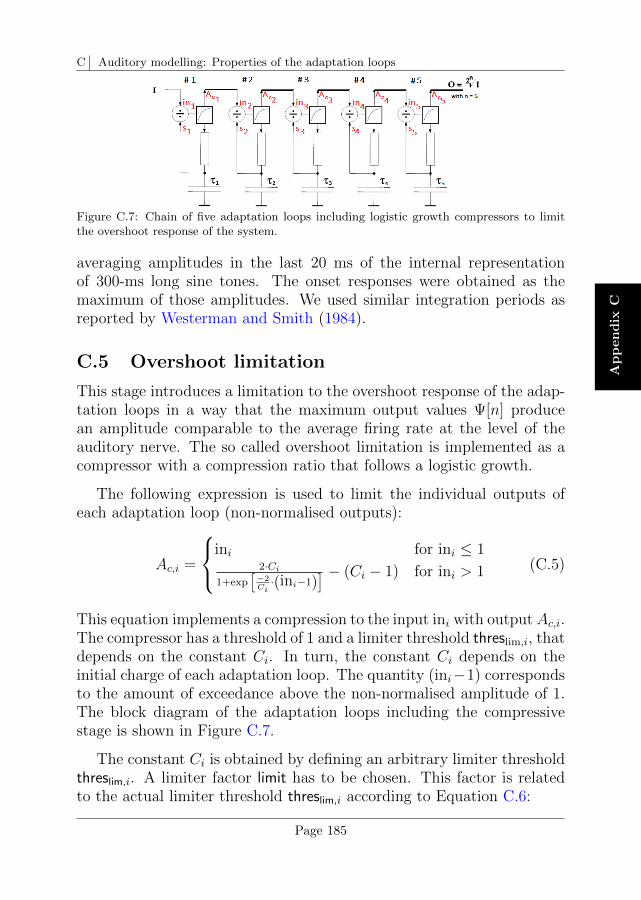
C Auditory modelling: Properties of the adaptation loops
Ap
pen
dix
C
Figure C.7: Chain of five adaptation loops including logistic growth compressors to limitthe overshoot response of the system.
averaging amplitudes in the last 20 ms of the internal representationof 300-ms long sine tones. The onset responses were obtained as themaximum of those amplitudes. We used similar integration periods asreported by Westerman and Smith (1984).
C.5 Overshoot limitation
This stage introduces a limitation to the overshoot response of the adap-tation loops in a way that the maximum output values Ψ[n] producean amplitude comparable to the average firing rate at the level of theauditory nerve. The so called overshoot limitation is implemented as acompressor with a compression ratio that follows a logistic growth.
The following expression is used to limit the individual outputs ofeach adaptation loop (non-normalised outputs):
Ac,i =
ini for ini ≤ 12·Ci
1+exp[−2Ci·(ini−1)
] − (Ci − 1) for ini > 1 (C.5)
This equation implements a compression to the input ini with outputAc,i.The compressor has a threshold of 1 and a limiter threshold threslim,i, thatdepends on the constant Ci. In turn, the constant Ci depends on theinitial charge of each adaptation loop. The quantity (ini−1) correspondsto the amount of exceedance above the non-normalised amplitude of 1.The block diagram of the adaptation loops including the compressivestage is shown in Figure C.7.
The constant Ci is obtained by defining an arbitrary limiter thresholdthreslim,i. A limiter factor limit has to be chosen. This factor is relatedto the actual limiter threshold threslim,i according to Equation C.6:
Page 185
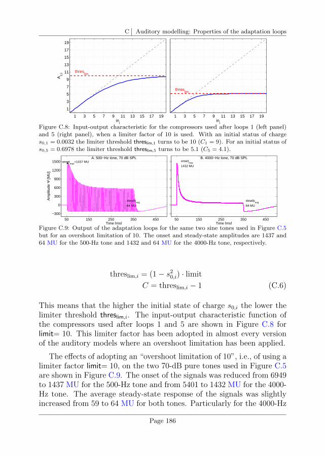
C Auditory modelling: Properties of the adaptation loops
1 3 5 7 9 11 13 15 17 19
1
3
5
7
9
11
13
15
17
19
threslim
ini
Ac,
i
Compression introduced in the OL (loop nr. 1)
1 3 5 7 9 11 13 15 17 19
1
3
5
7
9
11
13
15
17
19
threslim
ini
Ac,
i
Compression introduced in the OL (loop nr. 5)
Figure C.8: Input-output characteristic for the compressors used after loops 1 (left panel)and 5 (right panel), when a limiter factor of 10 is used. With an initial status of charges0,1 = 0.0032 the limiter threshold threslim,1 turns to be 10 (C1 = 9). For an initial status ofs0,5 = 0.6978 the limiter threshold threslim,5 turns to be 5.1 (C5 = 4.1).
50 150 250 350 450
−300
0
300
600
900
1200
1500
Time [ms]
Am
plitu
de Ψ
[MU
]
A. 500−Hz tone, 70 dB SPL
steadyavg
64 MU
onsetmax
=1437 MU
50 150 250 350 450
−300
0
300
600
900
1200
1500
Time [ms]
Am
plitu
de Ψ
[MU
]B. 4000−Hz tone, 70 dB SPL
steadyavg
64 MU
onsetmax
1432 MU
Figure C.9: Output of the adaptation loops for the same two sine tones used in Figure C.5but for an overshoot limitation of 10. The onset and steady-state amplitudes are 1437 and64 MU for the 500-Hz tone and 1432 and 64 MU for the 4000-Hz tone, respectively.
threslim,i = (1− s20,i) · limit
C = threslim,i − 1 (C.6)
This means that the higher the initial state of charge s0,i the lower thelimiter threshold threslim,i. The input-output characteristic function ofthe compressors used after loops 1 and 5 are shown in Figure C.8 forlimit= 10. This limiter factor has been adopted in almost every versionof the auditory models where an overshoot limitation has been applied.
The effects of adopting an “overshoot limitation of 10”, i.e., of using alimiter factor limit= 10, on the two 70-dB pure tones used in Figure C.5are shown in Figure C.9. The onset of the signals was reduced from 6949to 1437 MU for the 500-Hz tone and from 5401 to 1432 MU for the 4000-Hz tone. The average steady-state response of the signals was slightlyincreased from 59 to 64 MU for both tones. Particularly for the 4000-Hz
Page 186
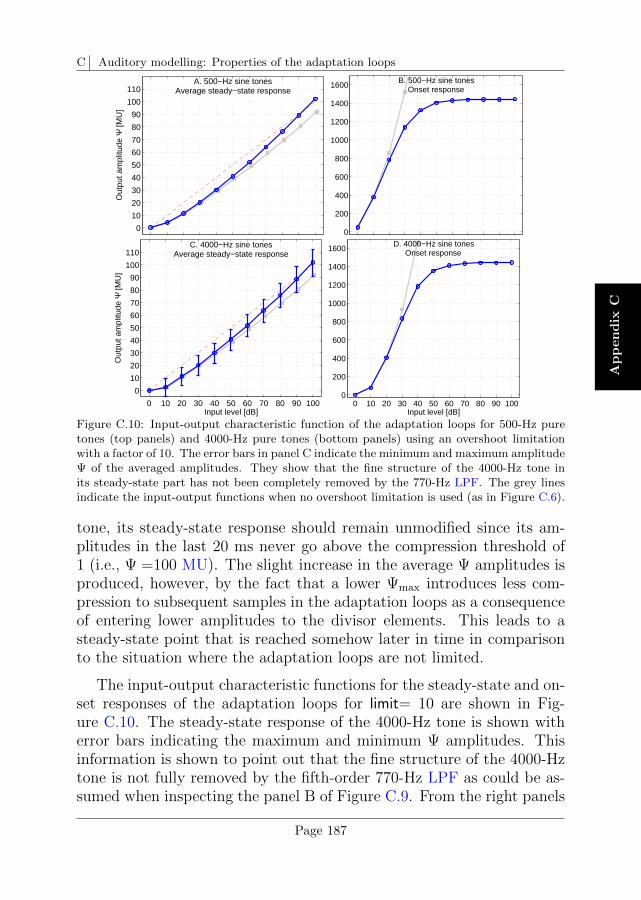
C Auditory modelling: Properties of the adaptation loops
Ap
pen
dix
C
0 10 20 30 40 50 60 70 80 90 100
0
10
20
30
40
50
60
70
80
90
100
110
Input level [dB]
Out
put a
mpl
itude
Ψ [M
U]
A. 500−Hz sine tonesAverage steady−state response
0 10 20 30 40 50 60 70 80 90 1000
200
400
600
800
1000
1200
1400
1600
Input level [dB]
Out
put a
mpl
itude
Ψ [M
U]
B. 500−Hz sine tonesOnset response
0 10 20 30 40 50 60 70 80 90 100
0
10
20
30
40
50
60
70
80
90
100
110
Input level [dB]
Out
put a
mpl
itude
Ψ [M
U]
C. 4000−Hz sine tonesAverage steady−state response
0 10 20 30 40 50 60 70 80 90 1000
200
400
600
800
1000
1200
1400
1600
Input level [dB]
Out
put a
mpl
itude
Ψ [M
U]
D. 4000−Hz sine tonesOnset response
Figure C.10: Input-output characteristic function of the adaptation loops for 500-Hz puretones (top panels) and 4000-Hz pure tones (bottom panels) using an overshoot limitationwith a factor of 10. The error bars in panel C indicate the minimum and maximum amplitudeΨ of the averaged amplitudes. They show that the fine structure of the 4000-Hz tone inits steady-state part has not been completely removed by the 770-Hz LPF. The grey linesindicate the input-output functions when no overshoot limitation is used (as in Figure C.6).
tone, its steady-state response should remain unmodified since its am-plitudes in the last 20 ms never go above the compression threshold of1 (i.e., Ψ =100 MU). The slight increase in the average Ψ amplitudes isproduced, however, by the fact that a lower Ψmax introduces less com-pression to subsequent samples in the adaptation loops as a consequenceof entering lower amplitudes to the divisor elements. This leads to asteady-state point that is reached somehow later in time in comparisonto the situation where the adaptation loops are not limited.
The input-output characteristic functions for the steady-state and on-set responses of the adaptation loops for limit= 10 are shown in Fig-ure C.10. The steady-state response of the 4000-Hz tone is shown witherror bars indicating the maximum and minimum Ψ amplitudes. Thisinformation is shown to point out that the fine structure of the 4000-Hztone is not fully removed by the fifth-order 770-Hz LPF as could be as-sumed when inspecting the panel B of Figure C.9. From the right panels
Page 187
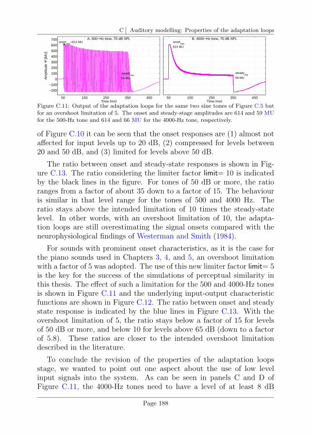
C Auditory modelling: Properties of the adaptation loops
50 150 250 350 450
−200
−100
0
100
200
300
400
500
600
700
Time [ms]
Am
plitu
de Ψ
[MU
]
A. 500−Hz tone, 70 dB SPL
steadyavg
59 MU
onsetmax
=614 MU
50 150 250 350 450
−200
−100
0
100
200
300
400
500
600
700
Time [ms]
Am
plitu
de Ψ
[MU
]
B. 4000−Hz tone, 70 dB SPL
steadyavg
66 MU
onsetmax
614 MU
Figure C.11: Output of the adaptation loops for the same two sine tones of Figure C.5 butfor an overshoot limitation of 5. The onset and steady-stage amplitudes are 614 and 59 MUfor the 500-Hz tone and 614 and 66 MU for the 4000-Hz tone, respectively.
of Figure C.10 it can be seen that the onset responses are (1) almost notaffected for input levels up to 20 dB, (2) compressed for levels between20 and 50 dB, and (3) limited for levels above 50 dB.
The ratio between onset and steady-state responses is shown in Fig-ure C.13. The ratio considering the limiter factor limit= 10 is indicatedby the black lines in the figure. For tones of 50 dB or more, the ratioranges from a factor of about 35 down to a factor of 15. The behaviouris similar in that level range for the tones of 500 and 4000 Hz. Theratio stays above the intended limitation of 10 times the steady-statelevel. In other words, with an overshoot limitation of 10, the adapta-tion loops are still overestimating the signal onsets compared with theneurophysiological findings of Westerman and Smith (1984).
For sounds with prominent onset characteristics, as it is the case forthe piano sounds used in Chapters 3, 4, and 5, an overshoot limitationwith a factor of 5 was adopted. The use of this new limiter factor limit= 5is the key for the success of the simulations of perceptual similarity inthis thesis. The effect of such a limitation for the 500 and 4000-Hz tonesis shown in Figure C.11 and the underlying input-output characteristicfunctions are shown in Figure C.12. The ratio between onset and steadystate response is indicated by the blue lines in Figure C.13. With theovershoot limitation of 5, the ratio stays below a factor of 15 for levelsof 50 dB or more, and below 10 for levels above 65 dB (down to a factorof 5.8). These ratios are closer to the intended overshoot limitationdescribed in the literature.
To conclude the revision of the properties of the adaptation loopsstage, we wanted to point out one aspect about the use of low levelinput signals into the system. As can be seen in panels C and D ofFigure C.11, the 4000-Hz tones need to have a level of at least 8 dB
Page 188
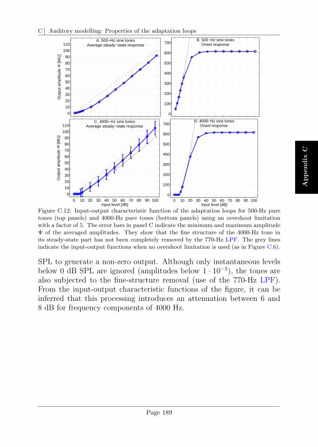
C Auditory modelling: Properties of the adaptation loops
Ap
pen
dix
C
0 10 20 30 40 50 60 70 80 90 100
0
10
20
30
40
50
60
70
80
90
100
110
Input level [dB]
Out
put a
mpl
itude
Ψ [M
U]
A. 500−Hz sine tonesAverage steady−state response
0 10 20 30 40 50 60 70 80 90 1000
100
200
300
400
500
600
700
Input level [dB]
Out
put a
mpl
itude
Ψ [M
U]
B. 500−Hz sine tonesOnset response
0 10 20 30 40 50 60 70 80 90 100
0
10
20
30
40
50
60
70
80
90
100
110
Input level [dB]
Out
put a
mpl
itude
Ψ [M
U]
C. 4000−Hz sine tonesAverage steady−state response
0 10 20 30 40 50 60 70 80 90 1000
100
200
300
400
500
600
700
Input level [dB]
Out
put a
mpl
itude
Ψ [M
U]
D. 4000−Hz sine tonesOnset response
Figure C.12: Input-output characteristic function of the adaptation loops for 500-Hz puretones (top panels) and 4000-Hz pure tones (bottom panels) using an overshoot limitationwith a factor of 5. The error bars in panel C indicate the minimum and maximum amplitudeΨ of the averaged amplitudes. They show that the fine structure of the 4000-Hz tone inits steady-state part has not been completely removed by the 770-Hz LPF. The grey linesindicate the input-output functions when no overshoot limitation is used (as in Figure C.6).
SPL to generate a non-zero output. Although only instantaneous levelsbelow 0 dB SPL are ignored (amplitudes below 1 · 10−5), the tones arealso subjected to the fine-structure removal (use of the 770-Hz LPF).From the input-output characteristic functions of the figure, it can beinferred that this processing introduces an attenuation between 6 and8 dB for frequency components of 4000 Hz.
Page 189
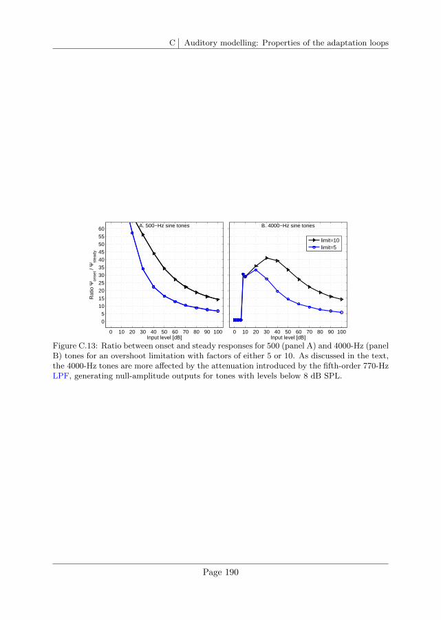
C Auditory modelling: Properties of the adaptation loops
0 10 20 30 40 50 60 70 80 90 100
0
5
10
15
20
25
30
35
40
45
50
55
60
Input level [dB]
Rat
io Ψ
onse
t / Ψ
stea
dy
A. 500−Hz sine tones
0 10 20 30 40 50 60 70 80 90 100
0
5
10
15
20
25
30
35
40
45
50
55
60
Input level [dB]
Rat
io Ψ
onse
t / Ψ
stea
dy
B. 4000−Hz sine tones
limit=10limit=5
Figure C.13: Ratio between onset and steady responses for 500 (panel A) and 4000-Hz (panelB) tones for an overshoot limitation with factors of either 5 or 10. As discussed in the text,the 4000-Hz tones are more affected by the attenuation introduced by the fifth-order 770-HzLPF, generating null-amplitude outputs for tones with levels below 8 dB SPL.
Page 190
D Auditory modelling: Calibration of theauditory model
In this appendix the procedure we followed to “calibrate” the auditory(PEMO) model used in Chapters 4 and 5 is described. The calibrationconsisted of finding a value for the variability σ of the internal (Gaussian)noise in a way that the performance of the artificial listener meets agiven criterion. More specifically, every time a parameter in the auditorymodel was added, removed, or modified, the variability σ of the internalnoise was adjusted (see Equation 4.5 in Chapter 4) to fulfil an intensity-discrimination task with a 70.7% score at a predefined test intensity.
In this appendix, two different σ values were used. A standard devi-ation σ = 3.4 MU was used to replicate simulation results of the PEMOmodel for the auditory tasks reported by Jepsen et al. (2008). A valueof σ = 10.1 MU was used to limit the performance of the artificial lis-tener to an intensity-discrimination task using piano sounds. The latterσ value was used to obtain the simulation results shown in Chapters 4and 5. In this appendix we do not provide a critical analysis of howsimilar our simulation results using the PEMO model are with respectto the results presented by Jepsen et al. (2008). The objective was toreplicate reported simulation results with the PEMO model as used inthis thesis. The interested reader may directly compare our results tothose presented by Jepsen et al. (2008).
D.1 Simulation procedure
All simulations reported in this appendix were run using the AFC toolboxfor MATLAB (Ewert, 2013). In this toolbox an artificial listener wasenabled to conduct the listening experiments presented in the subsequentsections. The artificial listener processed the incoming sounds using theauditory PEMO model. The experiments were all implemented as 3-AFC tasks using a two-down one-up tracking rule. Both the adjustable
Page 191
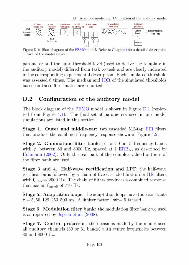
D Auditory modelling: Calibration of the auditory model
Figure D.1: Block diagram of the PEMO model. Refer to Chapter 4 for a detailed descriptionof each of the model stages.
parameter and the suprathreshold level (used to derive the template inthe auditory model) differed from task to task and are clearly indicatedin the corresponding experimental description. Each simulated thresholdwas assessed 6 times. The median and IQR of the simulated thresholdsbased on those 6 estimates are reported.
D.2 Configuration of the auditory model
The block diagram of the PEMO model is shown in Figure D.1 (replot-ted from Figure 4.1). The final set of parameters used in our modelsimulations are listed in this section.
Stage 1. Outer and middle-ear: two cascaded 512-tap FIR filtersthat produce the combined frequency response shown in Figure 4.2.
Stage 2. Gammatone filter bank: set of 30 or 31 frequency bandswith fc between 80 and 8000 Hz, spaced at 1 ERBN , as described byHohmann (2002). Only the real part of the complex-valued outputs ofthe filter bank are used.
Stage 3 and 4. Half-wave rectification and LPF: the half-waverectification is followed by a chain of five cascaded first-order IIR filterswith fcut-off= 2000 Hz. The chain of filters produces a combined responsethat has an fcut-off of 770 Hz.
Stage 5. Adaptation loops: the adaptation loops have time constantsτ = 5, 50, 129, 253, 500 ms. A limiter factor limit= 5 is used.
Stage 6. Modulation filter bank: the modulation filter bank we usedis as reported by Jepsen et al. (2008).
Stage 7. Central processor: the decisions made by the model usedall auditory channels (30 or 31 bands) with centre frequencies between80 and 8000 Hz.
Page 192
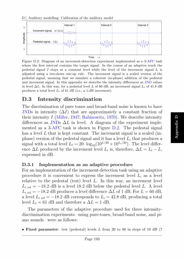
D Auditory modelling: Calibration of the auditory model
Ap
pen
dix
D
Increment signal, ∆ I (∆ L)
Pedestal signal, I (L)
Interval 1 Interval 2 Interval 3
Time →
←
A
mp
litu
de
→
Figure D.2: Diagram of an increment-detection experiment implemented as a 3-AFC taskwhere the first interval contains the target signal. In the course of an adaptive track thepedestal signal I stays at a constant level while the level of the increment signal Ii isadjusted using a two-down one-up rule. The increment signal is a scaled version of thepedestal signal, meaning that we simulate a coherent (in-phase) addition of the pedestaland increment signal. In this appendix we describe the intensity differences as JND valuesin level ∆L. In this way, for a pedestal level L of 60 dB, an increment signal Li of 41.8 dBproduces a total level Lt of 61 dB (i.e., a 1-dB increment).
D.3 Intensity discrimination
The discrimination of pure tones and broad-band noise is known to haveJNDs in intensity (∆I) that are approximately a constant fraction oftheir intensity I (Miller, 1947; Rabinowitz, 1970). We describe intensitydifferences as JNDs ∆L in level. A diagram of the experiment imple-mented as a 3-AFC task is shown in Figure D.2. The pedestal signalhas a level L that is kept constant. The increment signal is a scaled (in-phase) version of the pedestal signal and it has a level Li that produces asignal with a total level Lt = 20 · log10(10L/20 + 10Li/20). The level differ-ence ∆L produced by the increment level Li is, therefore, ∆L = Lt −L,expressed in dB.
D.3.1 Implementation as an adaptive procedureFor an implementation of the increment-detection task using an adaptiveprocedure it is convenient to express the increment level Li as a levelrelative to the pedestal (test) level L. In this way, an increment levelLi rel = −18.2 dB is a level 18.2 dB below the pedestal level L. A levelLi rel = −18.2 dB produces a level difference ∆L of 1 dB. For L = 60 dB,a level Li rel = −18.2 dB corresponds to Li = 42.8 dB, producing a totallevel Lt = 61 dB and therefore a ∆L = 1 dB.
The parameters of the adaptive procedure used for three intensity-discrimination experiments –using pure-tones, broad-band noise, and pi-ano sounds– were as follows:
• Fixed parameter: test (pedestal) levels L from 20 to 80 in steps of 10 dB (7
Page 193
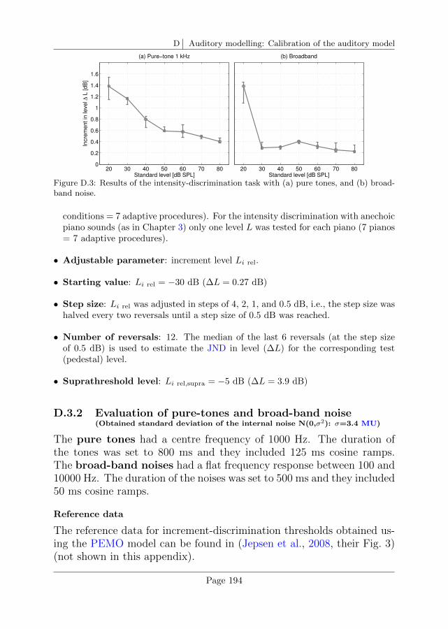
D Auditory modelling: Calibration of the auditory model
20 30 40 50 60 70 800
0.2
0.4
0.6
0.8
1
1.2
1.4
1.6
Standard level [dB SPL]
Incre
me
nt
in le
ve
l ∆ L
[d
B]
(a) Pure−tone 1 kHz
20 30 40 50 60 70 800
0.2
0.4
0.6
0.8
1
1.2
1.4
1.6
Standard level [dB SPL]
Incre
me
nt
in le
ve
l ∆ L
[d
B]
(b) Broadband
Figure D.3: Results of the intensity-discrimination task with (a) pure tones, and (b) broad-band noise.
conditions = 7 adaptive procedures). For the intensity discrimination with anechoicpiano sounds (as in Chapter 3) only one level L was tested for each piano (7 pianos= 7 adaptive procedures).
• Adjustable parameter: increment level Li rel.
• Starting value: Li rel = −30 dB (∆L = 0.27 dB)
• Step size: Li rel was adjusted in steps of 4, 2, 1, and 0.5 dB, i.e., the step size washalved every two reversals until a step size of 0.5 dB was reached.
• Number of reversals: 12. The median of the last 6 reversals (at the step sizeof 0.5 dB) is used to estimate the JND in level (∆L) for the corresponding test(pedestal) level.
• Suprathreshold level: Li rel,supra = −5 dB (∆L = 3.9 dB)
D.3.2 Evaluation of pure-tones and broad-band noise(Obtained standard deviation of the internal noise N(0,σ2): σ=3.4 MU)
The pure tones had a centre frequency of 1000 Hz. The duration ofthe tones was set to 800 ms and they included 125 ms cosine ramps.The broad-band noises had a flat frequency response between 100 and10000 Hz. The duration of the noises was set to 500 ms and they included50 ms cosine ramps.
Reference data
The reference data for increment-discrimination thresholds obtained us-ing the PEMO model can be found in (Jepsen et al., 2008, their Fig. 3)(not shown in this appendix).
Page 194
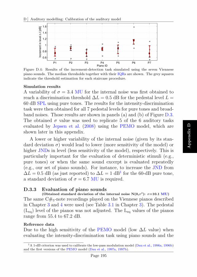
D Auditory modelling: Calibration of the auditory model
Ap
pen
dix
D
P1 P2 P3 P4 P5 P6 P7
0.6
0.8
1
1.2
1.4
1.6
Piano ID
Incre
ment in
level ∆
I [dB
]
Figure D.4: Results of the increment-detection task simulated using the seven Viennesepiano sounds. The median thresholds together with their IQRs are shown. The grey squaresindicate the threshold estimation for each staircase procedure.
Simulation results
A variability of σ = 3.4 MU for the internal noise was first obtained toreach a discrimination threshold ∆L = 0.5 dB for the pedestal level L =60 dB SPL using pure tones. The results for the intensity-discriminationtask were then obtained for all 7 pedestal levels for pure tones and broad-band noises. Those results are shown in panels (a) and (b) of Figure D.3.The obtained σ value was used to replicate 5 of the 6 auditory tasksevaluated by Jepsen et al. (2008) using the PEMO model, which areshown later in this appendix.
A lower or higher variability of the internal noise (given by its stan-dard deviation σ) would lead to lower (more sensitivity of the model) orhigher JNDs in level (less sensitivity of the model), respectively. This isparticularly important for the evaluation of deterministic stimuli (e.g.,pure tones) or when the same sound excerpt is evaluated repeatedly(e.g., our set of piano sounds). For instance, to increase the JND from∆L = 0.5 dB (as just reported) to ∆L = 1 dB1 for the 60-dB pure tone,a standard deviation of σ = 6.7 MU is required.
D.3.3 Evaluation of piano sounds(Obtained standard deviation of the internal noise N(0,σ2): σ=10.1 MU)
The same C#5-note recordings played on the Viennese pianos describedin Chapter 3 and 4 were used (see Table 3.1 in Chapter 3). The pedestal(Leq) level of the pianos was not adjusted. The Leq values of the pianosrange from 55.4 to 67.2 dB.
Reference data
Due to the high sensitivity of the PEMO model (low ∆L value) whenevaluating the intensity-discrimination task using piano sounds and the
1A 1-dB criterion was used to calibrate the low-pass modulation model (Dau et al., 1996a, 1996b)and the first versions of the PEMO model (Dau et al., 1997a, 1997b).
Page 195
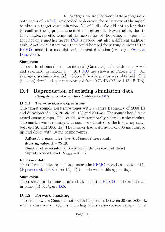
D Auditory modelling: Calibration of the auditory model
obtained σ of 3.4 MU, we decided to decrease the sensitivity of the modelto obtain a target discrimination ∆L of 1 dB. We did not collect datato confirm the appropriateness of this criterion. Nevertheless, due tothe complex spectro-temporal characteristics of the piano, it is possiblethat not only another target JND is needed but also a different auditorytask. Another auditory task that could be used for setting a limit to thePEMO model is a modulation-increment detection (see, e.g., Ewert &Dau, 2004).
Simulation
The results obtained using an internal (Gaussian) noise with mean µ = 0and standard deviation σ = 10.1 MU are shown in Figure D.4. Anaverage discrimination ∆L =0.86 dB across pianos was obtained. The(median) thresholds per piano ranged from 0.73 dB (P7) to 1.15 dB (P6).
D.4 Reproduction of existing simulation data(Using the internal noise N(0,σ2) with σ=3.4 MU)
D.4.1 Tone-in-noise experimentThe target sounds were pure tones with a centre frequency of 2000 Hzand durations of 5, 15, 20, 35, 50, 100 and 200 ms. The sounds had 2.5 msraised-cosine ramps. The sounds were temporally centred in the masker.The masker was a running Gaussian noise limited to the frequency rangebetween 20 and 5000 Hz. The masker had a duration of 500 ms rampedup and down with 10 ms cosine ramps.
Adjustable parameter: level L of target (tone) sounds.
Starting value: L = 75 dB.
Number of reversals: 12 (6 reversals in the measurement phase).
Suprathreshold level: L supra = 85 dB
Reference data
The reference data for this task using the PEMO model can be found in(Jepsen et al., 2008, their Fig. 4) (not shown in this appendix).
Simulation
The results for the tone-in-noise task using the PEMO model are shownin panel (a) of Figure D.5.
D.4.2 Forward maskingThe masker was a Gaussian noise with frequencies between 20 and 8000 Hzwith a duration of 200 ms including 2 ms raised-cosine ramps. The
Page 196
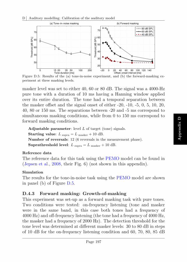
D Auditory modelling: Calibration of the auditory model
Ap
pen
dix
D
5 15 20 35 50 100 200
50
55
60
65
70
Tone duration [ms]
Th
resh
old
[d
B S
PL
]
(a) Tone−in−noise masking
−20 0 20 40 60 80 100 120 140
20
30
40
50
60
70
Offset−onset interval [ms]
Th
resh
old
[d
B S
PL
]
(b) Forward masking
80 dB SPL
60 dB SPL
40 dB SPL
Figure D.5: Results of the (a) tone-in-noise experiment, and (b) the forward-masking ex-periment at three masking levels.
masker level was set to either 40, 60 or 80 dB. The signal was a 4000-Hzpure tone with a duration of 10 ms having a Hanning window appliedover its entire duration. The tone had a temporal separation betweenthe masker offset and the signal onset of either -20, -10, -5, 0, 5, 10, 20,40, 80 or 150 ms. The separations between -20 and -5 ms correspond tosimultaneous masking conditions, while from 0 to 150 ms correspond toforward masking conditions.
Adjustable parameter: level L of target (tone) signals.
Starting value: L supra = L masker + 10 dB.
Number of reversals: 12 (6 reversals in the measurement phase).
Suprathreshold level: L supra = L masker + 10 dB.
Reference data
The reference data for this task using the PEMO model can be found in(Jepsen et al., 2008, their Fig. 6) (not shown in this appendix).
Simulation
The results for the tone-in-noise task using the PEMO model are shownin panel (b) of Figure D.5.
D.4.3 Forward masking: Growth-of-maskingThis experiment was set-up as a forward masking task with pure tones.Two conditions were tested: on-frequency listening (tone and maskerwere in the same band, in this case both tones had a frequency of4000 Hz) and off-frequency listening (the tone had a frequency of 4000 Hz,the masker had a frequency of 2000 Hz). The detection threshold for thetone level was determined at different masker levels: 30 to 80 dB in stepsof 10 dB for the on-frequency listening condition and 60, 70, 80, 85 dB
Page 197
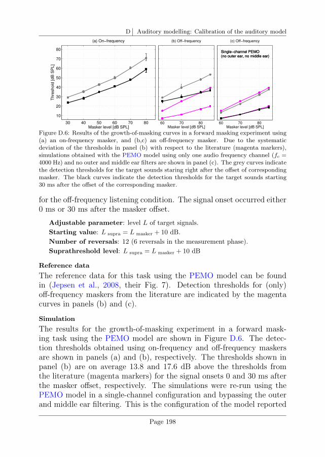
D Auditory modelling: Calibration of the auditory model
30 40 50 60 70 80
10
20
30
40
50
60
70
80
Masker level [dB SPL]
Th
resh
old
[d
B S
PL
]
(a) On−frequency
60 70 80
10
20
30
40
50
60
70
80
Masker level [dB SPL]
Th
resh
old
[d
B S
PL
]
(b) Off−frequency
60 70 80
10
20
30
40
50
60
70
80Single−channel PEMO(no outer ear, no middle ear)Single−channel PEMO(no outer ear, no middle ear)
Masker level [dB SPL]
Th
resh
old
[d
B S
PL
]
(c) Off−frequency
Figure D.6: Results of the growth-of-masking curves in a forward masking experiment using(a) an on-frequency masker, and (b,c) an off-frequency masker. Due to the systematicdeviation of the thresholds in panel (b) with respect to the literature (magenta markers),simulations obtained with the PEMO model using only one audio frequency channel (fc =4000 Hz) and no outer and middle ear filters are shown in panel (c). The grey curves indicatethe detection thresholds for the target sounds staring right after the offset of correspondingmasker. The black curves indicate the detection thresholds for the target sounds starting30 ms after the offset of the corresponding masker.
for the off-frequency listening condition. The signal onset occurred either0 ms or 30 ms after the masker offset.
Adjustable parameter: level L of target signals.
Starting value: L supra = L masker + 10 dB.
Number of reversals: 12 (6 reversals in the measurement phase).
Suprathreshold level: L supra = L masker + 10 dB
Reference data
The reference data for this task using the PEMO model can be foundin (Jepsen et al., 2008, their Fig. 7). Detection thresholds for (only)off-frequency maskers from the literature are indicated by the magentacurves in panels (b) and (c).
Simulation
The results for the growth-of-masking experiment in a forward mask-ing task using the PEMO model are shown in Figure D.6. The detec-tion thresholds obtained using on-frequency and off-frequency maskersare shown in panels (a) and (b), respectively. The thresholds shown inpanel (b) are on average 13.8 and 17.6 dB above the thresholds fromthe literature (magenta markers) for the signal onsets 0 and 30 ms afterthe masker offset, respectively. The simulations were re-run using thePEMO model in a single-channel configuration and bypassing the outerand middle ear filtering. This is the configuration of the model reported
Page 198
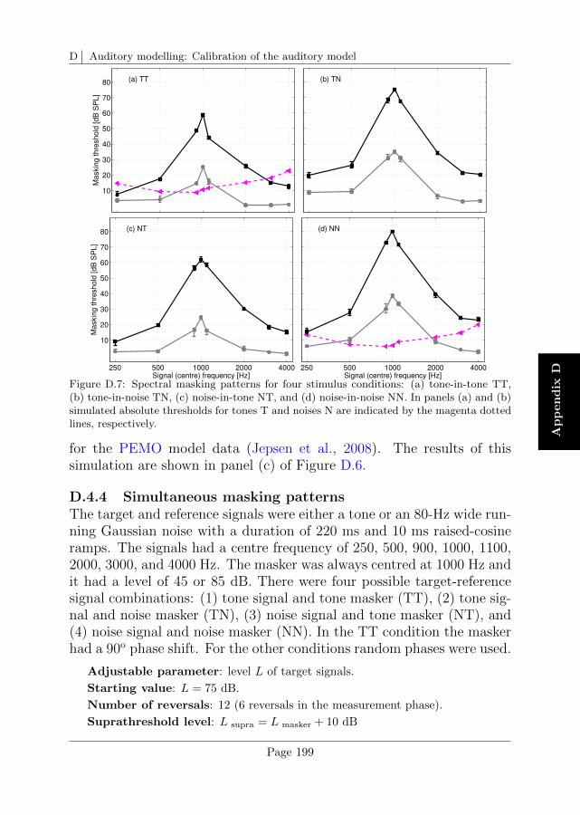
D Auditory modelling: Calibration of the auditory model
Ap
pen
dix
D
250 500 1000 2000 4000
10
20
30
40
50
60
70
80 (a) TT
Signal (centre) frequency [Hz]
Maskin
g thre
shold
[dB
SP
L]
250 500 1000 2000 4000
10
20
30
40
50
60
70
80 (b) TN
Signal (centre) frequency [Hz]
Maskin
g thre
shold
[dB
SP
L]
250 500 1000 2000 4000
10
20
30
40
50
60
70
80 (c) NT
Signal (centre) frequency [Hz]
Ma
skin
g t
hre
sh
old
[d
B S
PL
]
250 500 1000 2000 4000
10
20
30
40
50
60
70
80 (d) NN
Signal (centre) frequency [Hz]
Ma
skin
g t
hre
sh
old
[d
B S
PL
]
Figure D.7: Spectral masking patterns for four stimulus conditions: (a) tone-in-tone TT,(b) tone-in-noise TN, (c) noise-in-tone NT, and (d) noise-in-noise NN. In panels (a) and (b)simulated absolute thresholds for tones T and noises N are indicated by the magenta dottedlines, respectively.
for the PEMO model data (Jepsen et al., 2008). The results of thissimulation are shown in panel (c) of Figure D.6.
D.4.4 Simultaneous masking patternsThe target and reference signals were either a tone or an 80-Hz wide run-ning Gaussian noise with a duration of 220 ms and 10 ms raised-cosineramps. The signals had a centre frequency of 250, 500, 900, 1000, 1100,2000, 3000, and 4000 Hz. The masker was always centred at 1000 Hz andit had a level of 45 or 85 dB. There were four possible target-referencesignal combinations: (1) tone signal and tone masker (TT), (2) tone sig-nal and noise masker (TN), (3) noise signal and tone masker (NT), and(4) noise signal and noise masker (NN). In the TT condition the maskerhad a 90o phase shift. For the other conditions random phases were used.
Adjustable parameter: level L of target signals.
Starting value: L = 75 dB.
Number of reversals: 12 (6 reversals in the measurement phase).
Suprathreshold level: L supra = L masker + 10 dB
Page 199
D Auditory modelling: Calibration of the auditory model
Reference data
The reference data for this task using the PEMO model can be found in(Jepsen et al., 2008, their Fig. 5) (not shown in this appendix) and theyare reported as masked thresholds which are obtained as the detectionthresholds in dB SPL referenced to the absolute threshold of hearing forthe target signals.
Simulation
The results for the simultaneous-masking experiment using the PEMOmodel are shown in Figure D.7. The results are shown as masked thresh-olds in dB to allow a direct comparison with values from the literature.First the absolute thresholds for the target signals (tones T or noise N)centred at the test frequencies were obtained, which are indicated bythe magenta dotted lines in panels (a) and (d) for tone T and noise Ntargets. The masked thresholds were obtained by subtracting those ab-solute thresholds from the simulated detection thresholds for the fourtarget-reference signal combinations. The resulting curves are shown inpanels (a-d) for tone-in-tone, tone-in-noise, noise-in-tone, and noise-in-noise conditions, respectively.
Page 200
E Auditory modelling: Other approaches to assessthe memory template
This appendix contains a description of different template approachesthat were evaluated during the development of a central processor forthe PEMO model in the context of the perceptual similarity task de-scribed in Chapter 3 and simulated in Chapter 4. The finally adoptedtemplate approach is described in Chapter 4. This appendix is devotedto the description of those template approaches that did not lead to asatisfactory explanation of the experimental results of Chapter 3. Webelieve, however, that it is worthwhile to report these approaches indi-cating the reasons we had to leave them aside.
We start by providing some theoretical background behind the ideaof memory templates in the context of an optimal detector (see Green &Swets, 1966, their Chapters 6 and 7). This is followed by a description ofthe criteria we used to choose possible template approaches. We finallydescribe two of these alternative approaches and report the argumentthat lead us to discard them.
E.1 Theory for the derivation of a memorytemplate
In a 3-AFC task approached using an artificial listener (in this disserta-tion the PEMO model), the three trial intervals can be compared with an“expected signal” or template Tp. If the representations of each intervalare labelled as Rx with x = 1, 2, 3, then the template is derived from therepresentation that is related to the target sound (Rx,t) at a conditionthat is easy to discriminate, i.e., at a condition that is above threshold(suprathreshold condition). In a detection-in-noise experiment, such acondition is given when the background noise is low (i.e., high SNR)which, by convention, is indicated as Rx,t(MT ). In the course of a sim-ulated experiment the artificial listener chooses as target interval Rx,t
Page 201
E Auditory modelling: Other approaches to assess the memory template
(that may be correct or not) the interval that has the highest similaritywith Tp. One mathematical way to express this idea is to assess the CCVvalue between Rx and Tp. The expression to assess the CCV value incontinuous and discrete time domains is given by:
CCVx =
∫ T
0
Rx(t) · Tpdt ≈N∑n=1
Rx[n] · Tp[n]∆t (E.1)
In a simplified form:
CCVx =1
fs
N∑n=1
Rx[n] · Tp[n] (E.2)
where fs is the sampling frequency of the internal representations Rx
and Tp. The representations Rx and Tp are N -samples long. This op-eration can be interpreted as a “template weighting” and is referred inthe literature to as template-matching. The assessment of CCV valuescan in fact be performed along more dimensions of Rx and Tp as longas the samples Rx[n] and Tp[n] in the product of Equation E.2 belongto the same dimension. In general, the internal representations usingthe PEMO model have three dimensions: time, audio frequency, andmodulation frequency.
In Equation E.2, the template Tp sums up (or subtracts) the partsof the representation Rx that have the same (or a different) sign, em-phasising them (or de-emphasising them) by an amount defined by thesample-by-sample amplitudes of Tp. It is important to note that, in or-der to introduce an adequate weighting to the representation Rx, thetemplate Tp should have unit energy.
The template approaches described in this appendix consider differentways to use Equation E.2: (1) by using Rx (as shown in the equation) or∆Rx (i.e., subtracting the noise-alone representation), and (2) by usingsigned or unsigned samples in the equation.
E.1.1 Template weighting: Normalisation of the template
One property that has to be satisfied by the derived template Tp is tohave unit energy (Dau et al., 1996a):
E =
∫ T
0
T 2p (t)dt ≈ 1
fs
N∑n=1
T 2p [n] = 1 (E.3)
Page 202
E Auditory modelling: Other approaches to assess the memory template
Ap
pen
dix
E
where the left hand expression assumes a template Tp in the continuoustime domain and the right hand expression in the discrete time domain.The constants T and N represent the duration of the template in secondsand in samples, respectively. The discrete representation has a timeresolution ∆t = 1/fs [s], with fs being the sampling frequency of themodel representation in Hz.
To derive a template meeting the condition imposed by Equation E.3,a scaled representation of the target interval Rx,t(MT ) at a suprathresh-old SNR can be obtained. In this way, the template has the formTp = c ·Rx,t(MT ), and the constant c can be obtained as:
c =
√fs∑N
n=1R2x,t[n]
(E.4)
E.2 Criteria to be met
E.2.1 Template in a similarity task
The derivation of the template Tp in a similarity task where two (piano)sounds are compared, as described in Section 3.2.3, must be somehowrelated to: (a) the two test sounds, the target and “reference” pianos,and; (b) two or more realisations of a noise that can efficiently mask theproperties of both piano sounds. To account for the latter aspect, noiseis always added in every piano presentation (in this thesis they are ICRAnoises). For the first aspect, the internal representations of the targetpiano Rt needs to be used but the representation of the reference pianoRr might also be needed, because the discrimination between pianosdepends on how different they are from each other.
Finally, the internal representation of the noises alone RN mightalso be used in the template derivation. Despite the fact that in theinstrument-in-noise test, noise alone conditions are never presented, thelistener might be able to evaluate the similarity among intervals basedon how prominent the reference and target piano sounds are with respectto the (ICRA) noises.
E.2.2 Maximisation of the correlation between the templateand the internal representations
It is relevant that the template Tp is maximally correlated with each ofthe intervals Rx because it may be expected that human listeners try tomaximise the match between the expected signal (that we assumed to
Page 203

E Auditory modelling: Other approaches to assess the memory template
be “learned”) and each of the intervals that are heard. To maximise theCCV values, different time alignments of the involved internal represen-tations should be evaluated during either: (a) the template derivation,or (b) the correlation between the template and target and reference in-tervals. The relevance of this aspect relies on the fact that the templateTp and the representations Rx are digitised signals, which are sensitive toany eventual misalignment among them. This is in contrast to the ratio-nale of a memory template, where the awareness of the artificial listenerabout the target signal should be independent of the specific moment,i.e., the specific time alignment, when the test sounds are heard.
E.2.3 Compatibility of the template approach
The template approach should be compatible with the auditory tasksdescribed in Appendix D. This is motivated by the fact that a detection-in-noise task could also be seen as a similarity task, where a comparison ismade between the three intervals (signal-plus-noise and two noise-aloneintervals) and the template. The comparison is based on CCV valuesand the artificial listener chooses as the interval containing the targetsound the interval that produces the highest CCV value, i.e., the “mostsimilar” interval with respect to the template.
E.2.4 Adjustment of the sensitivity of the artificial listener
The use of different template approaches may introduce changes in thesensitivity of the artificial listener. To compensate for eventual changes inthe sensitivity of the artificial listener (i.e., the PEMO model), the vari-ability σ of the internal noise is checked and adjusted (if needed) by re-running the increment-detection experiment described in Section D.3.3.
E.3 Simulation procedure
All simulations were run using the AFC toolbox for MATLAB (Ewert,2013). In this toolbox an artificial listener was enabled to conductthe listening experiments. The artificial listener processed the (whole-duration) sounds using the auditory PEMO model with the set of param-eters listed in Chapter 4 using two overshoot limitation factors (limit= 10and limit= 5) in the adaptation loop stage. The experiments were all im-plemented as 3-AFC tasks using a two-down one-up tracking rule.
For each template approach, the experiments were always run in thefollowing order: (1) Increment-detection using C#5 (anechoic) piano
Page 204
E Auditory modelling: Other approaches to assess the memory template
Ap
pen
dix
E
sound (see Section D.3.3), (2) instrument-in-noise experiment, and (3)forward-masking experiments (see Section D.4.2). The first experimentwas run to assess the amount of variance σ needed for the internal noise ofthe central processor, the second experiment was run to evaluate the ar-tificial listener’s performance in our instrument-in-noise task. The thirdexperiment was run to evaluate the compatibility of the adopted ap-proach with the estimation of forward-masking thresholds. The forward-masking experiment was chosen with the motivation to replicate thethreshold estimation of one of the detection-in-noise tasks reported inAppendix D.
E.3.1 Stimuli
The same C#5-note (anechoic) recordings played on the Viennese pi-anos described in Chapter 3 and 4 were used for the simulation of theinstrument-in-noise experiment. Only a subset of 9 piano pairs (of the 21possible combinations) were used. The selected 9 piano pairs are well dis-tributed along the experimentally-obtained scale of similarity and theywere also used in the exploratory simulations presented in Chapter 4.The selected piano pairs were: pair 12, 15, 16, 23, 26, 27, 37, 45, and 47.
E.4 Approach 1: Piano-plus-noise templates
Description
In this approach one template is used. The template Tp is derived fromthe representation of the interval that contains the target piano sound(“target piano-plus-noise” interval). The approach is very similar to thederivation of templates that has been adopted so far in the literature(see, e.g., Dau et al., 1996b, 1997a; Jepsen et al., 2008). The targetpiano-plus-noise interval (presented once) is treated as the signal-plus-noise interval of a detection-in-noise experiment. Correspondingly thereference piano-plus-noise intervals (presented twice) are treated as thenoise-alone intervals of the detection task.
In this approach the CCV between the template Tp and the piano-plus-noise sounds for the intervals x = 1, 2, and 3 were obtained usingtwo variants:
CCVx =1
fs
N∑n=1
Rx[n] · Tp[n] (E.5)
and
Page 205
E Auditory modelling: Other approaches to assess the memory template
CCVx =1
fs
N∑n=1
∆Rx[n] · Tp[n] (E.6)
Criterion of the artificial listener
If interval x = 1 of the 3-AFC trial contains the target piano, then theartificial listener makes a correct decision if:
max
CCVx,t
= CCV1,t (E.7)
The hat symbol indicates that internal (Gaussian) noise N(0,σ2) is addedto the CCVx values before the artificial listener makes a decision.
Why not use this approach
The simulated thresholds thressim ranged from −7.0 to 2.5 dB for vari-ant 1 (Equation E.5) and from −3.5 to 5.5 dB for variant 2 (Equa-tion E.6). These reduced ranges of threshold values contrast with therange of experimental thresholds from thresexp,min= −1.75 dB and thresexp,
max= 20.75 dB that is reported in Chapter 3. Due to this large discrep-ancy and because in this approach the template derivation used only thetarget piano representation Rt, we decided to add explicit informationof the reference piano Rr in Approach 2.
E.5 Approach 2: Difference representation
Description
In this approach, the representation of the reference piano Rr is sub-tracted from the representation of the target piano Rt. The differencerepresentation ∆R = ‖Rt − Rr‖ is further analysed. The differencerepresentation is used now as a quantitative distance measure betweenrepresentations. Another study where an unsigned difference between in-ternal representations has also been used is given by Agus et al. (2012).The expression to assess the CCV values using the difference represen-tations has to be adjusted, because the artificial listener does not knowwhich interval contains the target and which of the other two intervalscontains the reference signals. The expression to obtain the CCV valuecan be written as follows:
CCVxy =1
fs
N∑n=1
‖∆Rxy[n]‖ · ‖Tp[n]‖ (E.8)
Page 206
E Auditory modelling: Other approaches to assess the memory template
Ap
pen
dix
E
the subindexes x and y indicate that the representation Ry from theinterval y is subtracted from the representation Rx from the interval x(∆Rxy = Rx −Ry).
Criterion of the artificial listener
Three CCV values are obtained using Equation E.8 using the internalrepresentations of intervals x = 1, 2, and 3 namely CCV12, CCV13, andCCV23. If the template Tp has also been derived from a difference rep-resentation between target and reference sounds, and we assume thatinterval 1 contains the target sound, then ∆R12 and ∆R13 should pro-duce a higher CCV than ∆R23. This is because ∆R23 does not accountfor the representation of the target sound. One way to translate this intoa discriminability outcome is to look for the lowest CCV value (in theexample CCV23). The artificial listener then chooses the “other” intervalas the target interval (in the example interval x = 1).
Why not use this approach
The simulated thresholds thressim had a similar range of values com-pared with those reported for the two variants of Approach 1, from −8.0to 3.75 dB. We faced, however, an additional problem for generatingdifference representations ∆Rxy namely to find out a systematic way ofensuring maximum (and reliable) CCV values between ∆Rxy and thetemplate. Different “types of difference representations” need to be gen-erated during the simulation of the similarity task, namely for (1) deriv-ing the template, (2) deriving the difference between target and referencerepresentations (R12 and R13), and (3) deriving the difference betweenreference representations R23. For each of those cases a different align-ment of the internal representations can increase or decrease the obtainedCCV values.
In order to try another approach where both the target and referencepiano representations can be used by the artificial listener but, at thesame time, reducing the dependency of the model judgements on find-ing an appropriate alignment criterion, we decided to adopt a criterionsimilar to that of Approach 1 but using two templates: Tp as in Ap-proach 1 (labelled as Tp,t) and another template derived in a similarway from the reference piano sound (labelled as Tp,r). Such a templatewas adopted and further investigated in Chapter 4.
Page 207
Acknowledgements
This dissertation is the end result of a four-years path along which I waslucky to always be surrounded by good people. Without all their supportthis project would have not been the same. For this reason I dedicate thefollowing lines to the many people who accompanied me along this path.
Firstly I would like to thank my supervisor. Armin, thank you forall the time you spent on our long weekly discussions, the enthusiasmthat you always showed and the flexibility to meet in different places atdifferent times not only including our offices but also our homes, cafesand restaurants. I believe this dissertation reflects many of the thingsthat I have learned from you in these four years.
I am also very grateful to my co-supervisor Antoine. I am very hon-oured to have worked with you. I loved working with your piano record-ings and to get familiar with some historical and technical facts aroundthe piano construction. You always made time for me even during yourbusy period in Vienna. I would also like to thank all other colleaguesand friends from our European project BATWOMAN especially Win-fried, Eckard, Sebastia and Malte.
Much of my gratitude goes to my colleagues and friends at the HTIgroup, for all the nice moments within and outside IPO. In particular Iwould like to thank Kong, Chao, Mark, Heleen, Giacomo, Kevin, Toros,Anne, Indre, Hanne, Maaike, Laura, Els, Elcin, Milou, Patty, Samantha,Minha, Caixia, Sofia, Alain, Peder, Anne M. and also to Leon, Sheng,Mieke, Mariska, Peter, Frank and Renske for the many coffees together,walks around, Cookie Wednesdays, and other spontaneous get-togethers.I am also thankful for the open-door approach in our group and for thehelp that I repeatedly got from Ellen, Dik, Daniel, Peter, Raymond,Martin and Aart. My office mates also deserve a special mention: Ryan,Huihui, Nemanja, Rebecca, Sima and Margot. Thank you for the goodtime at IPO 0.21. I would also like to thank the students I had theopportunity to supervise in particular Rodrigo, Kevin and Glen, whocollected part of the data used in this thesis.
Page 208
Acknowledgements
During my Ph.D. I regularly travelled between Antwerp and Eind-hoven. Despite the long travelling times, I can count two positive conse-quences. The first one is that I was able to meet two very good friends.Ake en Casimir, it is nice to realise that although you do not need tocome to Eindhoven anymore, we have managed to keep the contact witheach other. The second consequence was that I got to know bettersome Eindhoven-friends every time I could benefit from their hospitality.Those stays in Eindhoven were most of the times complemented witheither dinners, drinks, Champions League matches or a combination ofthem. Thank you Kong, Toros, Peder, Edgar and Llaima.
Federico and Michael, I am also grateful to you and our long lastingfriendship. I do not only enjoy every time we meet, but I also get inspiredwhen we discuss about our ongoing research or any other “geek” stuff.
I am eternally grateful to my family in Chile. My parents Luis andAlicia have always stayed close to me despite the long distance that sep-arates us. Papito y mamita, muchas gracias por el apoyo incondicionalque siempre me han dado, gracias por todos los sacrificios que ustedeshicieron para que yo llegue a donde estoy, ustedes siempre han sido yseguiran siendo mi ejemplo a seguir. Thank you Carolina and Robertofor shortening the long distance with our spontaneous chats. Caro, gra-cias por siempre hacerme partıcipe de tu vida, incluso ahora que estamostan lejos. Me siento orgulloso de que ahora estes haciendo lo que real-mente te gusta y de la vida que estas formando con Manuel. Rober, losultimos anos te han tocado duro, pero pese a eso siempre has estadocuando lo he necesitado. Me alegro de verte junto a Monica y de tusahora tres preciosos hijos Leon, Matıas y Rafael.
I am also grateful to my in-laws, mijn schoonouders Gilbert en Gert,mijn schoonbroers en hun wederhelft Jeroen en Karen, Stijn en Iris, mijnschoonnichtjes (echt schoon) Jade, Linde en Evelyn en mijn neef (ook heelschoon) Lenn. Jullie hebben me met open armen ontvangen en aanvaardzonder daar iets voor terug te vragen. Bedankt voor jullie steun.
Finally I would like to thank my wife Frauke. We have done so muchin the last years. You and our two beautiful children Paula and Alexisare for me the biggest source of inspiration, motivating me to becomeevery day better. Pinguinita, gracias por estar a mi lado. Tu apoyo,comprension, empatıa, amistad y cercanıa me hacen un mejor hombre,padre, persona y tambien investigador. Por esto, sin darte cuenta, tueres quien mas ha contribuido al trabajo que presento en esta tesis.
Page 209
Curriculum Vitae
Alejandro Osses Vecchi was born on 20 May 1985 in Santiago, Chile. Heobtained the professional degree of civil engineer in sound and acous-tics in 2010 at the Technological University of Chile INACAP (formerVicente Perez Rosales). He then worked in the area of environmentalacoustics as project manager and project engineer at the consultancycompanies Acustical (2010-2012) and Control Acustico (2011-2012), re-spectively. In 2012 he moved to Belgium, where he completed a pre-doctoral programme in biomedical sciences at the University of Leuven.The topic of his research project was concerned with real-time audiosignal processing for cochlear implants. Since May 2014 Alejandro ispart of the Human-Technology Interaction group at the Eindhoven Uni-versity of Technology where he started a Ph.D. project under the su-pervision of prof. Armin Kohlrausch. The project titled “Prediction ofperceptual similarity based on time-domain models of auditory percep-tion” was performed within the Initial Training Network BATWOMANin the framework of a Marie Sk lodowska-Curie Action, with the main goalto stimulate interdisciplinary research among three disciplines –musicalacoustics, room acoustics, and automotive applications– with perceptionas a central focus.
Page 210
Publications
Peer reviewed papers
A. Osses, and A. Kohlrausch (2018, submitted). “Auditory modelling of the percep-tual similarity between piano sounds.” Acta Acust. united Ac.
A. Chaigne, A. Osses, and A. Kohlrausch (2018, submitted). “Similarity of pianotones: a psychoacoustical and sound analysis study.” Applied Acoustics.
A. Osses, A. Kohlrausch, W. Lachenmayr, and E. Mommertz (2017). “Predicting theperceived reverberation in different room acoustic environments using a binaural audi-tory model.” J. Acoust. Soc. Am. 141(4), pp. EL381-EL387. doi:10.1121/1.4979853.
Papers in preparation
A. Osses, A. Kohlrausch, and A. Chaigne. “Perceptual similarity between pianonotes: Experimental data for reverberant and non-reverberant sounds.”
A. Osses, and A. Kohlrausch. “Perceptual similarity between piano notes: Simula-tions with a template-based perception model.”
Non-peer reviewed papers
A. Osses, A. Chaigne, and A. Kohlrausch (2017). “Meten van klankverschillen inklassieke piano’s” (Measurement of sound differences in classic pianos, in Dutch).Nederlands Tijdschrift voor Natuurkunde 83 (7), pp. 246-249.
Osses, A., Chaigne, A. and Kohlrausch, A. (2016). Assessing the acoustic similarityof different pianos using an instrument-in-noise test. International Symposium onMusical and Room Acoustics, pp. 1-10. La Plata, Argentina. (Link to download)
Osses, A., Garcıa, R. and Kohlrausch, A. (2016). “Modelling the sensation of fluctu-ation strength. Proc. Mtgs. Acoust. 28 (50005), pp. 1-8. doi:10.1121/2.0000410.
A. Osses, C. Kim, and A. Kohlrausch (2015). “Perceptual evaluation of differencesbetween original and synthesised musical instrument sounds: the role of room acous-tics.” Proceedings of EuroNoise. Ed. by C. Glorieux. Maastricht, the Netherlands,pp. 2561-2566. (Link to download)
Page 211

Colophon
This thesis was typeset using LATEX. Thecover of this dissertation was designedby Carolina Osses Vecchi. This disserta-tion was printed by: ProefschriftMaken ‖www.proefschriftmaken.nl
Page 212
Related Documents