Prediction of oil yield from oil shale minerals using diffuse reflectance infrared Fourier transform spectroscopy

Prediction of oil yield from oil shale minerals using diffuse

reflectance infrared Fourier transform spectroscopy

Mike J. Adamsa, Firas Awajaa, Suresh Bhargavaa,*, Stephen Grocottb, Melissa Romeoc

aApplied Chemistry, Science, Engineering and Technology Portfolio, RMIT University, P.O. Box 2476V, Melbourne, Vic. 3001, AustraliabBHP Billiton Technology, Newcastle Technology Centre, off Vale st. Shortland, NSW 2307, Australia

cDepartment of Chemistry and Biochemistry, Hunter College, 695 Park Avenue, New York, NY 10021, USA

Received 18 February 2005; accepted 14 April 2005

Available online 23 May 2005

Abstract

Multivariate analysis techniques, principal component analysis (PCA), principal component regression (PCR) and partial least square

regression (PLSR), were employed to develop calibration and prediction models for the determination of oil yield from oil shale samples

using diffuse reflectance infrared Fourier transform spectroscopy (DRIFTS). Data pre-processing included the use of second-derivative

spectral data. Multi-component models were constructed and were effective in predicting oil yield with accurate predictions achieved using

oil shale samples other than those used in the calibration set. DRIFTS with multivariate calibration modelling is demonstrated to provide a

simple and rapid method of evaluating oil yield from oil shales compared with, and potentially replacing, the traditional modified Fisher

assay (MFA) method.

q 2005 Elsevier Ltd. All rights reserved.

Keywords: Oil shale; Oil yield prediction; DRIFTS; PLSR; PCA

1. Introduction

The rising consumption and increasing price of pet-

roleum-based products have prompted extensive studies for

alternative sources of this material. The extraction and

production of oil from oil shale is one alternative available

in Australia and other regions in the world. Oil shales are a

fine-grained sedimentary rock containing relatively large

amount of organic matter (kerogen) that can be converted to

oil by thermal degradation of the crushed rock [1,2]. The

evaluation of the amount of oil that can be produced from oil

shale is decisive in controlling the process and is

traditionally determined using a modified Fisher assay

(MFA) technique [3].

The evaluation of oil yield in oil shale samples using the

MFA method is time consuming and expensive, involving

pyrolysis at 500 8C with the liberated hydrocarbons

collected as vapour and condensed. As a means of

0016-2361/$ - see front matter q 2005 Elsevier Ltd. All rights reserved.

doi:10.1016/j.fuel.2005.04.011

* Corresponding author. Tel.: C61 3 99253365; fax: C61 3 96391321

E-mail address: [email protected] (S. Bhargava).

monitoring potential oil-yield for management and control

of the commercial process the MFA method lacks speed of

analysis and, as an assay method, the MFA procedure is

susceptible to poor reproducibility between analysts and

apparatus employed. For at-line or on-line analysis, large

numbers of shale samples need to be tested to determine the

validity of oil shale mining and processing from a particular

seam or deposit. To overcome these problems, DRIFTS has

been proposed as a cheaper, faster and non-destructive

means of evaluating oil yield from oil shale [4,5].

Isolation of the appropriate IR bands and quantifi-

cations of a sample’s organic content is complicated by

the high mineral content of the shales. Previous studies

have relied on a ‘spectral stripping’ procedure to isolate

the aliphatic hydrocarbon region of the infrared spectrum.

This technique, relying on sequential subtraction of

interfering mineral and organic component spectra from

a sample’s spectrum, is complex and demands a detailed

knowledge of a sample’s composition for accurate results

[4–6].

An alternative procedure, applied here, is to employ

multivariate modelling techniques to analyse the complete

infrared spectral data. Combining DRIFTS with multi-

variate calibration, and generating a model to predict oil

Fuel 84 (2005) 1986–1991

www.fuelfirst.com

M.J. Adams et al. / Fuel 84 (2005) 1986–1991 1987

yield directly from oil shale samples, can facilitate

the processing of oil shale, and the procedure has the

potential to be implemented in situ and replace the

traditional MFA method.

Multivariate calibration serves as a tool for analysing

large sets of data such as generated by spectroscopic

analysis. Multivariate calibration models using principal

components regression (PCR) or partial least square

regression (PLSR) algorithms have widespread application

in spectral analysis and their application is described in

detail elsewhere [7–9]. PCR combines principal com-

ponent analysis (PCA) spectral decomposition with

inverse least squares regression to create a calibration

model suitable for complex samples. The PCR method

regress the analyte concentrations on the PCA scores.

PLSR is closely related to PCR, but the spectral

decomposition process includes the analyte concentration

values and spectra of those samples containing higher

analyte concentrations are weighted more heavily. Thus,

PLSR takes advantage of the correlations between spectral

data and constituent concentrations. In both cases, the data

matrix of spectral response values is decomposed to

generate new variables that are linear combinations of the

original measured variables. The aim of both methods is

to develop a calibration model containing fewer indepen-

dent variables than would be possible using conventional

multiple linear regression techniques. Both PCR and

PLSR techniques have been applied to the determination

of oil yield from oil shale using DRIFTS data and we

report here the results obtained and an interpretation of

these results and the models developed.

Fig. 1. Typical oil sh

2. Experimental

2.1. Samples

Oil shale samples were obtained from the Stuart oil shale

deposit, Queensland, Australia (Southern Pacific Petroleum

Co., Australia). All samples (50 for developing a calibration

model and a further 37 samples for subsequent validation)

were supplied with oil-yield values determined independently

using the MFA technique. Samples analysed had reported oil-

yield values in the range 50–300 L/ton. Each sample received

(200 g) was mixed thoroughly and a 3–4 g portion separated

and ground in an orbital steel ring grinder for 30 s.

2.2. DRIFTS

Shale sub-samples were put into a diffuse reflectance cup

(10 mm diameter, 3.3 mm depth) and a constant packing

density ensured by applying a fixed mass (30 g) on the top

surface of each sample. The infrared spectrum of each sub-

sample was recorded using a model 2000 FT-IR spec-

trometer (Perkin–Elmer, UK) fitted with a Praying Mantis

diffuse reflectance attachment (Harrick Scientific, NY,

USA). The spectra were recorded at 16 cmK1 spectral

resolution in the region 4000–586 cmK1 relative to a KBr

background producing 215 values recorded as pseudo-

absorbance (log 1/R) values for each spectrum. Once a

spectrum was recorded the reflectance cup was rotated

through 908 and a second spectrum recorded. This procedure

was undertaken on two sub-samples from each ground shale

ale spectrum.

M.J. Adams et al. / Fuel 84 (2005) 1986–19911988

sample, producing four spectra from each sample, which

were averaged to provide the modelling data.

2.3. Data processing and analysis

All programs and data analysis algorithms were devel-

oped and applied in-house using MathCad (Vs 11.0

Mathsoft Eng. Inc., Cambridge, MA, USA). Background

correction to minimise assumed scattering effects was

achieved using a 9-point second-derivative quadratic

function and PCR and PLSR undertaken using the NIPALS

and the SIMPLS algorithms, respectively [10–14].

3. Results and discussion

A set of 50 oil shale samples, with corresponding MFA

data, was used for experimental analysis and the develop-

ment of calibration models. A typical oil shale spectrum is

shown in Fig. 1 and the major components identified.

0

0.2

0.4

0.6

0.8

1

1.2

1.4

1.6

1.8

2(a)

(b)

2500300035004000

Ab

sorb

ance

-4

-3

-2

-1

0

1

2

3

2500300035004000

Aliphatic hydrocarbon 2930 cm-1

Kaolinite3700 cm-1

Wavenu

Wavenumb

Ab

sorb

ance

(2n

d D

eriv

ativ

e)

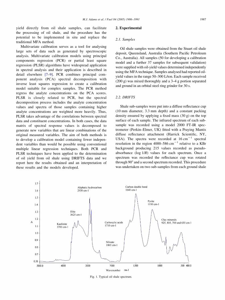
Fig. 2. (a) DRIFTS spectra of 10 oil shale samples of var

The spectrum comprises aliphatic and aromatic stretching

and bending vibrations from kerogen overlapped with

contributions from the minerals present, in particular

carbonates and quartz. A sharp band at 3700 cmK1 has

been attributed to kaolinite, the sharp band at 3625 cmK1

arises from illite in the shale [15]. The broad O–H band at

3370 cmK1 is also attributed to kaolinite, with possible

contribution from moisture in the shale, absorbed during

sample preparation. The broad O–H band obscures aromatic

C–H vibrations, expected around 3030 cmK1. Aliphatic

hydrocarbon stretching bands are observed at 2930 cmK1

(yas CH2) and (ys CH2) [16]. Snyder et al. [5] employed

derivative methods to identify the number of bands actually

present in these two peaks. The C–H stretching region was

resolved into five bands, with contributions from asym-

metric (2956 cmK1) and antisymmetric (2872 cmK1)

methyl stretching vibrations as well as contributions from

lone C–H group (2895 cmK1), couples with overtones and

combinations of bending modes near 1450 cmK1. A small

peak observed at 1865 cmK1 is most likely an overtone or

500100015002000

500100015002000

Aromatic C= C 1640 cm-1

AliphaticHydrocarbon1456 cm-1

Quartz800 cm-1

Hydroxyl, ester and ether 1288 cm

mber (cm-1)

er (cm-1)

-1

ying oil yield and (b) the second derivative spectra.

1

1.5

2

2.5

3

3.5

50 100 150 200 250 300 350

Ab

sorb

ance

(ar

ea)

MFA (T/L)

Fig. 3. Absorbance area around 2935 cmK1 vs. MFA value for 50 oil shale

samples.

0

5

10

15

20

25

30

35

40

45

RMSEC

RMSEP

Number of components0 1 2 3 4 5 6 7

Err

or(

L/T

)

Fig. 5. Error vs. number of component for the PCR model.

M.J. Adams et al. / Fuel 84 (2005) 1986–1991 1989

combination band of the silicate mineral fundamental. A

shoulder observed at 1710 cmK1, due to carboxylic acids in

kerogen, is not completely resolved as a strong band at

1640 cmK1 (aromatic and olefinic carbon–carbon double

bond) overlaps [16,17]. The band at 1640 cmK1 masks any

spectral contribution from aromatic carbon vibrations. The

broad band at 1460 cmK1 arises from methyl and methylene

deformation modes, with overlap from carbonate minerals.

The three unresolved bands at 1190, 1160 and 1105 cmK1

are characteristic of pyrite. The bands in the region 1000–

450 cmK1 are due to clay and minerals in the oil shale, in

particular quartz, with characteristic silicate vibrations

occurring at 505 and 450 cmK1.

The band at 2930 cmK1 is associated with aliphatic

hydrocarbons present in the sample and is assumed to be

correlated with the sample’s kerogen content [4,6]. Fig. 2(a)

shows the spectra of 10 oil shale samples with varying oil

yield value. The variations in intensity of the 2930 cmK1

-50

-40

-30

-20

-10

0

10

20

30

40

50

-50 -30 -10 10 30 50

PC 1

PC2

Fig. 4. Projected second derivative IR spectra on the first and second

principal components.

band with changing MFA value as well as the considerable

variation in baseline of the spectra due to scatter effects are

evident.

The absorption band near 2930 cmK1 increases in

relative intensity with increasing MFA value. The peak

area of this band, determined using a linear baseline

between 3000 and 2800 cmK1, vs. MFA value is presented

in Fig. 3. This univariate calibration curve has a goodness of

fit (r2) value of 0.687 and a root mean square error of

calibration (RMSEC) of 37.511 L/ton. This simple cali-

bration model has been discussed by Solomon and Mikinis

[4] and Cronauer et al. [6]. These authors showed how better

correlation can be achieved by replacing MFA value by total

organic carbon content. The inclusion of other structural

organic components in the correlation and the identification

and minimisation of mineral interference would be expected

to result into a more accurate and precise calibration model.

However, the overlapping mineral bands limit the appli-

cation of this simple model.

0

5

10

15

20

25

30

35

40

45

Err

or

RMSEC

RMSEP

Number of components0 1 2 3 4 5 6 7

Fig. 6. Error vs. number of component for the PLSR model.

0

50

100

150

200

250

300

0 50 100 150 200 300

Pre

dic

ted

MF

A

250

Actual MFA

Fig. 7. Predicted vs. actual MFA for PLSR model with four components,

RMSEPZ19.11.

M.J. Adams et al. / Fuel 84 (2005) 1986–19911990

Before developing and applying PCR and PLSR models,

the spectral data was transformed by application of a 9-point

quadratic second-derivative filter in order to remove the

severe baseline effects. Fig. 2(b) shows the second

derivative spectra of the 10 spectra shown in Fig. 2(a).

Although the spectra are less easy to interpret, compared

with the original data, the reduction in baseline effects is

evident.

The 2930 cmK1 band is strongly present in the derivative

spectra and other significant spectral peaks can be identified,

for example near 3700 cmK1 assigned to kaolinite,

1645 cmK1 assigned to aromatic and olefinic carbon double

bond, 1456 cmK1 assigned to aliphatic hydrocarbons (CH2

groups contribution), 1288 cmK1 assigned to hydroxyl,

ester and ether groups, 1155 cmK1 assigned to olefinic

groups and the 800 cmK1 band which is assigned to quartz.

The second derivative data were variable mean-centred

and principal component analysis performed. The first two

factors (principal components) accounted for 61% of the

variance in the data and are plotted in Fig. 4.

-2.5

-2

-1.5

-1

-0.5

0

0.5

1

1.5

2

2500300035004000

Reg

ress

ion

co

effi

cien

t

Kaolinite

Wavenum

Aliphatic hydrocarbon

Fig. 8. Regression coefficients derived fro

PCR analysis was undertaken between the reported MFA

oil-yield values and selected principal components. A

calibration model employing principal components was

developed by adding the factors one at a time to a linear

model and determining at each stage the root mean square

error of calibration (RMSEC) using the 50 samples in the

training set, and the root mean square error of prediction

(RMSEP) using the spectra from 37 samples not used for

calibration. The factors were included in the model

according to their correlation with MFA oil yield values.

The results are shown in Fig. 5 and indicate a 5-component

model is adequate for prediction.

In some cases, PLSR can show significant improvement

in calibration modelling compared with PCR, and the

technique was examined here using the SIMPLS algorithm.

Fig. 6 shows RMSEC and RMSEP values as a function of

number of factors included in the PLS regression model. As

with PCR, a 4-component model appeared optimal for

calibration and the error of calibration (RMSECZ13.8 L/

ton) is significantly better than that obtained using PCR

(RMSECZ16.3 L/ton). Fig. 7 shows the predicted vs.

anticipated oil-yield values. With 4 factors in the PLSR

model, the final regression coefficients across the spectral

region are shown graphically in Fig. 8.

As to be expected the intensity of the peak near

2930 cmK1 has a significant effect and this aliphatic

hydrocarbon band represents a major feature in the

regression model. The other aliphatic hydrocarbon band

near 1436 cmK1 was not affecting significantly the model.

Another strong variable is evident at 1645 cmK1. This band

is associated with the aromatic and olefinic carbon double

bond contribution. The band near 1568 cmK1 wavenumber

that might be associated to carbonate is also noticeable. This

suggests a contribution of carbonate minerals in the accurate

estimation of oil content. Significant contribution also is

noticed from the variable at 1705 cmK1 wavenumber. This

band is associated with carboxyl groups. The clay-

associated peaks are also present especially near 1088 and

736 cmK1. The characteristic double peak near 800 cmK1

wavenumber which is assigned to quartz is present.

500100015002000

Aromatic C=C

Carbonate

Quartz

Clay and minerals

ber (cm-1)

Carboxyl group

m the 4-components PLSR model.

M.J. Adams et al. / Fuel 84 (2005) 1986–1991 1991

The kaolinite assignment at 3700 cmK1 wavenumber is also

represented in the model. Most variables that were

described in Figs. 2 and 4 affects MFA value.

4. Conclusion

Multivariate calibration modelling has proved to be

effective and efficient tool combined with DRIFTS for

predicting oil content from oil shale. Models constructed

using PCR and PLSR show high calibration and prediction

ability, with PLSR exhibiting superior prediction perform-

ance. Low RMSEP values for shale oil content were obtained

using a 4-component PLSR model. The PLSR model can be

used with DRIFTS to provide a low cost technique to

facilitate the in situ prediction of oil from shale samples.

Acknowledgements

Authors wish to acknowledge Southern Pacific Pet-

roleum and the Australian Research Council for their

financial support.

References

[1] El harfi K, Mokhlisse A, Ben Chanaa M. J Anal Appl Pyrolysis 2000;

56:207–18.

[2] Jaber JO, Probert SD. Fuel Process Technol 2000;63:57–70.

[3] Shadle LJ, Seshardi KS, Webb DL. Fuel Process Technol 1994;37:

101–20.

[4] Solomon PR, Miknis FP. Fuel 1980;12:893–6.

[5] Snyder RW, Painter PC, Conauer DC. Fuel 1983;62:1205–14.

[6] Cronauer DC. Am Chem Soc Div Fuel Chem 1982;122–30.

[7] Martens H, Naes T. Multivariate calibration. New York: Wiley;

1989.

[8] Beebe RK, Pell RJ, Seasholtz MB. Chemometrics: a practical guide.

New York: Wiley; 1998.

[9] Wold, S., Trygg, J., Berglund, A. H. Antti 58; 2001. p. 131–50.

[10] Lorber A, Wangen LE, Kowalski BR. J Chemom 1987;1:19–31.

[11] Thomas EV. Anal Chem 2000;72(13):2821–7.

[12] Savitzky A, Golay MJE. Anal Chem 1964;36:1627–39.

[13] de Jong S. Chemom Intell Lab Syst 1993;18:251–63.

[14] Madden HH. Anal Chem 1978;50:1383–9.

[15] Gadsden, J.A. Infrared spectra of minerals and related inorganic

compounds, Butterworth, MA; 1975.

[16] Bruan V, Halim M, Ziyad M, Largeau M, Ambles C. J Anal Appl

Pyrolysis 2001;61(1–2):165–79.

[17] Grice K, Schouten S, Blokker P, Derenne S, Largeau C,

Nissenbaum A, et al. Org Geochem 2003;34:471–82.