Prediction of Fatigue Strength in Steels by Linear ...

Prediction of Fatigue Strength in Steels by Linear Regression and Neural Network

Takayuki Shiraiwa+1, Yuto Miyazawa+2 and Manabu Enoki

Department of Materials Engineering, The University of Tokyo, Tokyo 113-8656, Japan

This paper examines machine learning methods to predict fatigue strength with high accuracy using existing database. The fatigue databasewas automatically classified by hierarchical clustering method, and a group of carbon steels was selected as a target of machine learning. In linearregression analyses, a model selection was conducted from all possible combinations of explanatory variables based on cross validationtechnique. The derived linear regression model provided more accurate prediction than existing empirical rules. In neural network models, localand global sensitivity analyses were performed and the results of virtual experiments were consistent with existing knowledge in materialsengineering. It demonstrated that the machine learning method provides prediction of fatigue performance with high accuracy and is one ofpromising method to accelerate material development. [doi:10.2320/matertrans.ME201714]

(Received May 29, 2018; Accepted June 18, 2018; Published July 23, 2018)

Keywords: steel, fatigue strength, linear regression, neural network, model selection, machine learning, materials integration

1. Introduction

Structural materials are mostly used for a long time and thetime-dependent performances such as fatigue, creep andcorrosion are directly related to the safety of our infra-structure. As a demand of new materials for specificapplications increases and the cost of the experiments toevaluate the time-dependent performances rises, it isbecoming increasingly important to reduce the number ofexperiments in the material development process. Againstsuch a background, many attempts have been made todevelop a methodology for predicting the fatigue perform-ances by using physical models, numerical simulation,empirical rules and machine learning. In order to capturethe complicated relationship between the manufacturingconditions and the performance, it is effective to decomposethe material system into four principal elements of process,structure, properties and performance and to create modelsfor each relationship.1) By integrating these models, theperformance prediction can be realized.2­5) Despite a greatdeal of effort using computational simulations,6­8) there isstill a lack of models that predict dislocation structureformation and microstructurally small crack growth undercyclic loading, and it is still challenging to develop themethodology to predict the total fatigue life with the currenttheoretical understanding. The need to bridge models of theelementary processes over different length scales and timescales makes the fatigue prediction more difficult. Althoughthe empirical rules can be one way to obtain the missingmodels, the present measurement techniques do not providesufficient data to derive the empirical models for dislocationand crack initiation.

In contrast, vast amounts of data on the process-performance relationship have been accumulated over theyears for engineering applications. These data are not helpfulfor understanding the elementary processes of fatigue but areuseful for interpolative prediction of performance within alimited range of materials. With the rapid improvement of

computer performance and development of software,numerous machine learning algorithms have been proposedover several decades. In the traditional approach, we mustselect an appropriate learning algorithm to solve a problemfrom the set of the numerous algorithms, and choose theexplanatory variables from many features in database. Thistraditional approach has resulted in successful predictionsin various fields. In the field of mechanical properties,Mukherjee et al.9) proposed a multivariate regression modelto predict the hardness of thermo-mechanically treated rebarsas a function of chemical composition and temperingparameters. Ozerdem and Kolukisa10) predicted multiplemechanical properties of copper alloy by using neuralnetwork. Collins et al.11) utilized Bayesian neural networkto predict tensile properties of Ti­6Al­4V alloys with highaccuracy. Also in the case of fatigue prediction, theseapproaches have been adopted. Malinov et al.12) developedneural network models to predict various mechanicalproperties including fatigue strength for titanium alloys.Agrawal et al.13) compared many kinds of machine learningalgorithms for the prediction of fatigue strength in steels.Results of these researches showed that the accuracy of theprediction of fatigue strength was lower than that of othermechanical properties such as tensile strength and hardness.This can be explained by the fact that fatigue involvesmore complex interactions between microstructure, stressand environment than static mechanical properties. A moresophisticated approach is required for fatigue prediction.

The purpose of this paper is to examine machine learningmethods suitable for fatigue problems and to predict fatiguestrength with high accuracy using existing database. Thedatabase contains fatigue properties on various kinds ofmaterials. Since the mechanism of fatigue failure differs frommaterial to material, empirical formulas should be derivedseparately for each material group. For this reason, the fatiguedataset was automatically classified by hierarchical clusteringmethod, and a group of carbon steels was selected as a targetof machine learning. After data preprocessing, there remained393 samples with 21 explanatory variables such as chemicalcompositions, process parameters, heat treatment conditionsand inclusion parameters, and one objective variable offatigue strength. In linear regression analyses, a model

+1Corresponding author, E-mail: [email protected]+2Graduate Student, The University of Tokyo. Present address: IHICorporation, Yokohama 235-8501, Japan.

Materials Transactions, Vol. 60, No. 2 (2018) pp. 189 to 198Special Issue on Development of Materials Integration in Structural Materials for Innovation©2018 The Japan Institute of Metals and Materials

selection was conducted from all possible combinations ofexplanatory variables based on cross validation technique inorder to minimize the prediction error. In neural networkmodels, a suitable network topology and an appropriateactivation function were examined. Comparing the linearregression and neural network models, the advantage anddisadvantage of each model were discussed. Also, by usingthese models, local and global sensitivity analyses wereperformed to evaluate the significance of each explanatoryvariable on the fatigue strength.

2. Methods

2.1 DataFatigue data sheet (FDS) provided from national institute

of material science (NIMS)14) was used, which is one of theworld’s largest fatigue databases and contains general steels,stainless steels, cast irons, aluminum alloys, nickel alloys,titanium alloys and magnesium alloys. In total, 689 types ofmetallic materials are linked to the features including fatiguestrength, chemical compositions, processing parameters, heattreatment conditions, inclusion parameters and grain size.The chemical composition consists of 25 different elements:Fe, C, Si, Mn, P, S, Ni, Cr, Cu, Mo, Al, N, B, Nb, Ti, W, V,Co, Sb, O, Sn, Mg, Zn, Zr and H. The processing parametersinclude reduction ratio and heat treatment parameters inpre-heating, normalizing, quenching, tempering, annealing,solution and aging. The inclusion parameters are area fractionof inclusions deformed by plastic work (dA), inclusionsoccurring in discontinuous arrays (dB) and isolatedinclusions (dC). The grain size is recorded for ferrite andprior austenite in several steels, and primary ¡ andtransformed ¢ phase of titanium alloy. The fatigue strengthwas determined at 107 cycles in rotating bending fatigue testsunder room temperature.

2.2 Hierarchical clustering and data preprocessingThe fatigue dataset was classified purely based on

chemical composition by hierarchical clustering method inorder to avoid the artificial categorization. Clustering isone of unsupervised learning methods and classifies datapoints into different data aggregates, that is, clusters. Amongvarious clustering methods, hierarchical clustering iscapable of grouping data points on various scales bycreating a dendrogram, and is considered to be effectivefor classification of metal materials. Hierarchical clusteringalgorithms are categorized into agglomerative (bottom-up)and divisive (top-down).15) In the current study, thishierarchical agglomerative clustering was performed withthe 689 material samples using the 25 chemical contents asexplanatory variables.

It is obvious that the result of the clustering depends onthe definitions of distance between data points (intra-cluster distance) and distance between clusters (inter-clusterdistance). In order to determine the optimum definitions,clustering analyses were performed with all materials in thedatabase by changing the definitions of intra-cluster andinter-clusters, and it was evaluated whether five kinds ofmetal materials (iron alloy, aluminum alloys, nickel alloys,titanium alloys and magnesium alloys) can be divided into

each cluster. The mean, minimum and maximum values ofthe parameters used for the clustering analysis is shown inTable 1. Euclidean distance, standardized Euclidean distanceand Mahalanobis distance16) were used as the intra-elementdistances. Given a dataset comprising n samples of X =(x1, x2,+, xn)T and each sample has p explanatory variablesxi = (xi1, xi2,+, xip)T, the distances between the data points xiand xj are defined as follows:

dEuclidij ¼ffiffiffiffiffiffiffiffiffiffiffiffiffiffiffiffiffiffiffiffiffiffiffiffiffiffiffiffiffiXpk¼1

ðxik � xjkÞ2s

; ð1Þ

dstandard Euclidij ¼

ffiffiffiffiffiffiffiffiffiffiffiffiffiffiffiffiffiffiffiffiffiffiffiffiffiffiffiffiffiffiffiffiffiXpk¼1

xik � xjk·k

� �2

vuut ; ð2Þ

dMahalanobisij ¼

ffiffiffiffiffiffiffiffiffiffiffiffiffiffiffiffiffiffiffiffiffiffiffiffiffiffiffiffiffiffiffiffiffiffiffiffiffiffiffiffiffiffiffiffiffiðxi � xjÞ��1ðxi � xjÞT

q; ð3Þ

where ·k is the standard deviation of feature k, C is thecovariance matrix of the entire data X. The inter-clusterdistance was calculated by shortest distance method,farthest distance method,17) group average method,18) Ward’smethod19) and centroid distance method.20) In the shortestdistance method, the distance between the closest two datapoints belonging to two clusters is measured. Conversely, thefarthest distance method uses the distance between the mostdistant two data points. The group average method uses anaverage value of distances for all the combinations of twodata points belonging to two clusters. The Ward’s methodmerges the clusters to minimize the difference between the

Table 1 Mean, minimum and maximum values of explanatory variablesused for clustering analysis.

T. Shiraiwa, Y. Miyazawa and M. Enoki190

variance of the cluster after merging and the sum of varianceof clusters before merging. The centroid method uses thedistance between the centroids of clusters. Using three intra-cluster distances and five inter-cluster distances, clusteringanalyses were performed with a total of 15 algorithms. Toassess the quality of the clustering, entropy was calculatedfor five clusters derived by each algorithm. The entropy ofcluster, H, was defined by the following equation:

½p1; p2; . . . ; pK� ¼jCðk; 1ÞjjCðkÞj ; . . . ;

jCðk;KÞjjCðkÞj

� �; ð4Þ

HðCðkÞÞ ¼ �XKk¼1

pk logpk; ð5Þ

where k is cluster index, K is number of clusters (K = 5),«C(k)« is the number of data points belonging to cluster k,«C(k, j)« is the number of data points corresponding tomaterial j (iron alloy, aluminum alloys, etc.) in cluster k. Lowentropy indicates high quality clustering.15) The total entropyof five clusters was compared among the algorithms todetermine the optimal definitions of intra-cluster distance andinter-cluster distance.

Using the determined definitions of distances, 630 types ofiron alloys in the database were clustered. In the NIMSfatigue data sheet, iron alloys are classified into 15 categoriesof bearing steel, carbon steel for machine structural use,carbon steel for pressure vessels, Cr steel, Cr­Mo steel, Cr­Mo­V steel, ferritic heat-resisting steel, heat-resisting steel,Mn steel, Ni­Cr steel, Ni­Cr­Mo steel, spring steel, stainlesssteel, tool steel and spheroidal graphite cast iron. To comparewith these categories, the maximum number of clusters wasset to 15. As the details are to be mentioned in section 3.1,509 types of steels were classified into one cluster, and wereused in the following data preprocessing.

2.3 Data preprocessingIn the fatigue database, not all features exist for all

materials. In order to reduce the number of explanatoryvariables and not to reduce the number of material samples asmuch as possible, the data was preprocessed as follows:(1) Alloying elements whose content is 0mass% in all 630

steels were excluded from the explanatory variables.(2) Material samples subjected to heat treatment other than

quenching, tempering and normalizing were excluded.These three heat treatments have two variables oftemperature T (K) and time t (min). These two variableswere summarized into one variable of T log(t). Formaterials not quenched or tempered, T log(t) = 0 wasassigned.

(3) The grain size of ferrite and austenite were excludedfrom the explanatory variables because only either ofthem was recorded in the most cases. Since primary ¡

and transformed ¢ phase of titanium alloy do not existin steels, they were excluded.

After the preprocessing, there remained 21 explanatoryvariables of reduction ratio, dA, dB, dC, Fe, C, Si, Mn, P, S,Ni, Cr, Cu, Mo, Al, N, Ti, O, normalizing, quenching andtempering. The number of materials was 393. The mean,maximum, and minimum values of each explanatory variableare shown in Table 2. These 393 samples were randomly

divided into training dataset with 360 samples and test datasetwith 33 samples to evaluate the accuracy of linear regressionmodel.

2.4 Linear regression modelLinear regression is one of the simplest and powerful

regression method in which the relationship betweenexplanatory and objective variables is modelled by a linearequation. Multivariate linear regression model can beexpressed as follows:

y ¼Xpi

aixi; ð6Þ

where y is objective variable, xi is explanatory variable and aiis constant coefficient for explanatory variables xi. Althoughmore complex model gives more accurate prediction in thetraining dataset, if the model is too complex, the accuracyin the validation dataset decrease due to over-fitting.21) Toavoid this problem, a variable selection from all 221 ¹ 1combinations of explanatory variables was conducted tominimize the validation error based on cross validationtechnique. The procedure of the cross validation is illustratedin Fig. 1. At first, 360 training samples were divided forevery ten into 36 groups. Linear regression coefficients werecalculated for 35 groups except the first group and fatiguestrength of first group was predicted by using thesecoefficients. Then, root mean squared error (RMSE) of thisprediction was calculated. After that, 35 groups except thesecond group were used to calculate coefficients and RMSEwas calculated for the second groups. Repeating theseprocedures, 36 values of RMSE were calculated and total

Table 2 Mean, minimum and maximum values of explanatory variablesused for training, validation and testing. The fifth column representsselected variables and coefficient ai of linear regression model.

Prediction of Fatigue Strength in Steels by Linear Regression and Neural Network 191

RMSE was recorded as cross validation error (CVE). Thecross validation was performed for all 221 ¹ 1 combinationsof explanatory variables.

2.5 Neural network model2.5.1 Architecture

Artificial neural network is one way of machine learningwhich is inspired by biological neural networks. Thearchitecture of artificial neural network used is depictedin Fig. 2(a). In each unit of hidden and output layers,calculation was conducted as following equation and theresult was sent to next layer.

hj ¼ ¤Xk

wjkxk þ bj

!; ð7Þ

where xk is the input variable from kth unit in input layer, wjk

and bk are weight and bias, hj is the output variable, and ¤ isactivation function. Changing the training algorithms, datanormalization method, activation function and number ofhidden layers (one or two layers), the prediction accuracy inthe test dataset was compared. The number of units in eachlayer was fixed to be ten units on the first hidden layer andfive units on the second hidden layer.

2.5.2 Activation functionIn the output layer, identity function ¤(x) = x was used

as activation function. In hidden layers, three kinds ofnon-linear function were used as shown in the followingequations and Fig. 2(b):

¤ðxÞ ¼ 1

1þ e�x; ð8Þ

¤ðxÞ ¼ tanhðxÞ ¼ ex � e�x

ex þ e�x; ð9Þ

ºðxÞ ¼ maxð0; xÞ: ð10ÞEquation (8) represents sigmoid function. It was commonlyused early in neural network research because it is simple andeasy to differentiate. Equation (9) is a hyperbolic tangent.Glorot and Bordes22) showed that the hyperbolic tangent ismore suitable for neural network than the sigmoid function.Equation (14) is a ramp function. In neural network research,this function is called as “Rectified Linear Unit” or “ReLU.”Glorot and Bengio23) showed that ReLU is better than thehyperbolic tangent. LeCun et al.24) reported that ReLU is thebest activation function as of May 2015.2.5.3 Data normalization

When using sigmoid function or hyperbolic tangent as theactivation function, output value converges to «1 or 0 asthe input value moves far from zero. It means that thesignificance of input variable is almost eliminated. To solvethis problem, the input and output variables should benormalized. In this research, three methods of normalizationwere examined. The first normalization method (hereinaftercalled “n1”) is to normalize so that the average becomes zeroand the variance becomes one as follows:

x0i ¼xi � �x

·; ð11Þ

where xAi is the normalized variable, �x is the mean value and sis standard deviation. LeCun et al.25) suggested that thismethod was the best for neural network. The second and thirdmethod (hereinafter called “n2” and “n3”) are to normalize sothat the range of xAi becomes [0, 1] and [0.1, 0.9], respectively:

x0i ¼xi � xmin

xmax � xmin

; ð12Þ

x0i ¼ 0:1þ ð0:9{0:1Þ � xi � xmin

xmax � xmin

; ð13Þ

where xmax and xmin are maximum and minimum value of eachexplanatory variable. Sobhani et al.26) used eq. (13) for theneural network model.2.5.4 Training algorithm

Training of neural network is to properly set weights andbiases. The backpropagation algorithm is one of the mostcommon training methods. At the beginning of training

Fig. 1 Schematic representation of the cross-validation method.

(a)

(b)

-2

-1.5

-1

-0.5

0

0.5

1

1.5

2

-3 -2 -1 0 1 2 3

SigmoidTanhReLU

x

φ (x)

Input layer Hidden layer 1 Hidden layer 2 Output layerxk

1 ≤ k ≤ phj

1 ≤ j ≤ 10hi

1 ≤ i ≤ 5y

wjk wijwli bl

bibj

Fig. 2 (a) Architecture of artificial neural network and (b) activationfunctions.

T. Shiraiwa, Y. Miyazawa and M. Enoki192

process, random values are assigned to weights and biases.The output value is calculated by using these initial weightsand biases. Comparing the output value with experimentalvalue, the bias of the output layer and the weight from thehidden layer are updated. Then, comparing the value of thehidden unit with the previous value, the bias of the hiddenlayer and the weight from the former layer are updated. In asimilar manner, all weights and biases are updated. One cyclethat updates weights and thresholds in all layers is called oneepoch. Thus, the error in the output layer propagates to theinput layer through the network, and hence this method iscalled as backpropagation.

The goal of the backpropagation is to minimize the error.In general, the error is the sum of squared errors between thepredicted value and the actual value. To minimize the sum ofsquares, many algorithms have been proposed. The gradientdescent method and the Gauss-Newton method are popularalgorithm to solve this problem. The gradient descent methodrequires a long time to converge and the Gauss-Newtonmethod converges quickly but can give inaccurate results.Consequently, the Levenberg-Marquardt (LM) method27)

which is a combination of the gradient descent method andthe Gauss-Newton method was adopted. Training wasstopped when either the average error on the training datasetswas less than a preset value, Marquardt parameter exceeded1.0 © 1010, or the number of epochs exceeded 5000. Thedataset was randomly divided into 70% for training, 15% forvalidation and 15% for testing when using LM method.

To prevent over-fitting, Bayesian framework has beenproposed for the training in neural network.28) In theframework, the goal of training is to minimize the functionE(w) shown below, instead of sum squared error,

EðwÞ ¼ ¢EDðwÞ þ ¡EwðwÞ; ð14Þ

EDðwÞ ¼1

2

Xnk¼1

ðyk � okÞ2; ð15Þ

EwðwÞ ¼1

2

Xi

wi2; ð16Þ

where yk is predicted value, ok is observed value (actualvalue), w is vector of weights and biases. ED(w) is an errorfunction similar to the total squared error in LM method.Ew(w) is called a penalty term, which encourages to lower theweights and suppresses over learning. The calculation wasperformed based on LM method. The coefficients ¡ and ¢ arehyper parameters to control the complexity of model. If ¢ istoo large, the degree of freedom of the model becomes largeand over-fitting occurs. Conversely, if ¡ is too large, theweights and biases are not fitted to the data. To address thisproblem, the two parameters were statistically determinedby Bayes’ theorem.29) The Bayes’ theorem is represented asfollows:

pðw;DÞ ¼ pðwjDÞpðDÞ ¼ pðDjwÞpðwÞ; ð17Þwhere D is data set. When w is the most probable, p(w«D)becomes maximum. p(w«D) is in proportion to twoprobabilities:

pðwjDÞ / pðDjwÞpðwÞ: ð18ÞAssuming that these two probabilities are normal distributions,

pðDjwÞ ¼Ynk¼1

pðokjxk;wÞ

¼ 1

ZDexp � 1

2·v2

Xnk¼1

ðyk � okÞ2( )

;

¼ 1

ZDexp � 1

·v2ED

� �ð19Þ

pðwÞ ¼ 1

Zwexp � 1

2·w2kwk2

� �

¼ 1

Zwexp � 1

·w2Ew

� �; ð20Þ

pðwjDÞ / 1

ZDZwexp � 1

·v2ED þ 1

·w2Ew

� �� �; ð21Þ

where ZD and Zw are constants for normalization, ·v is thestandard deviation of actual output values, and ·w is thestandard deviation of weights and biases. Maximizing p(w«D)is equivalent to minimizing (ED/·v

2 + Ew/·w2). Comparing

with eq. (14), two coefficients ¡ and ¢ are determined fromthe standard deviations. According to MacKay,30) there is noneed to prepare validation data in the Bayesian framework.Therefore, the data set were chosen randomly for 85% fortraining and 15% for testing. These two training algorithm,LM method and LM method with Bayesian framework, werecompared.2.5.5 Evaluation

Training conditions are summarized in Table 3. Thetraining algorithm was evaluated with model 1 and 2 in thetable. All nine combinations of the three types of activationfunction and the three normalization method described inprevious sections were compared using model 3 to 11. Sincethe result varied depending on the data dividing, ten trainingdatasets were prepared by randomly dividing the entire dataten times. Each dataset was named as dataset number 1 to 10.In order to further improve the prediction accuracy, a secondhidden layer was added to the selected neural networkmodel (model 12). In each model, epoch number, correlationcoefficient between actual value and predicted value oftraining data, validation data, test data and all data wererecorded.

Table 3 Training conditions for neural network models. H1 and H2represent the number of hidden layers, and LM is Levenberg-Marquardt(LM) method, and LM+Bayes is LM method with Bayesian framework.

Prediction of Fatigue Strength in Steels by Linear Regression and Neural Network 193

2.5.6 Sensitivity analysisSensitivity analysis (SA) is to evaluate the contribution

of input uncertainty to output uncertainty of model.31) Thesensitivity is divided into local sensitivity and globalsensitivity. The local sensitivity refers to the sensitivity at afixed point in the parameter space, while global sensitivityrefers to an integrated sensitivity over the entire inputparameter space.32) In the linear regression model, thecoefficient directly represents the local and global sensitivity,as shown in the eq. (6). In contrast to the linear regressionmodel, weights and biases in neural network model havecomplicated influences on the sensitivity. The localsensitivity can be evaluated by changing only one of theexplanatory variables and fixing remaining variables. Severalresearchers call the local SA in neural network model as“virtual experiment.”11) However, it does not represent theoverall significance of the explanatory variables over theentire data. To evaluate the significance on fatigue strengthover a wider range of materials, global SA is required. Usingthe created neural network model, global SA was performedby combined weight method,33) fourier amplitude sensitivitytest (FAST) method34,35) and Sobol’ method.36,37) Also, thelocal SA was conducted to examine the effect of carbon andmanganese contents on the fatigue strength.

3. Results and Discussions

3.1 Hierarchical clusteringTotal entropy of five clusters is shown in Fig. 3. Among

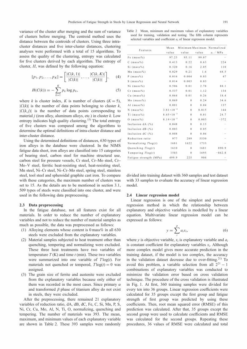
the three intra-cluster distances of Euclidean, standardizedEuclidean, and Mahalanobis distance, five metallic materialswere successfully clustered with Euclidean distances. Of thefive inter-cluster distances, the shortest distance method,the group average method, and the center of gravity methodprovided successful clustering. In the centroid method,the dendrogram partially reversed and intersected. This isbecause the centroid of cluster moved due to cluster mergingand the distance between clusters does not monotonicallydecrease. Based on these results, the shortest distancemethod with Euclidean distance was used in the subsequentclustering.

Results of hierarchical clustering of 630 iron alloys into15 clusters using shortest distance method with Euclideandistance are shown in Fig. 4. The horizontal axis representsthe distance in the chemical composition space, that is,dissimilarity of chemical composition. In this analysis, 509alloys of 630 alloys were classified into one cluster. Thecluster contained carbon steels and low-alloy steels withsmall amounts of Cr, Mn, Mo and Ni. Such classification wasquite different from 15 categories in the NIMS fatigue datasheet. It indicated that it is necessary to add the informationof heat treatment, microstructure and properties in order toperform clustering matching the existing database.

3.2 Linear regression modelResult of variable selection with cross validation method is

shown in Fig. 5. The horizontal axis shows the number ofexplanatory variables, p, and the vertical axis shows theminimum CVE for each number of explanatory variables. Itcan be seen that CVE reached a minimum at p = 14. Selectedvariables and calculated coefficients are shown in Table 2.Variables of C, Si, Mn, P, Ni, Cr, Cu, Mo, Al, N, Ti, O,quenching, tempering were selected. All of these variablesare selected more than 85 times in the top 100 combinations.The normalized coefficients showed that two heat treatmentshave great significance on the fatigue strength. Also, theresult showed that fatigue strength increases by addingelements of C, Mn and Cu, which is consistent with our

AverageWard Centroid Shortest Farthest

0

0.05

0.1

0.15

0.2

0.25

0.3

0.35

0.4EuclideanStandardized EuclideanMahalanobis

Tota

l ent

ropy

of f

ive

clus

ters

Definition of inter-cluster distanceFig. 3 Effect of distance definition on total entropy in hierarchical

clustering of metallic materials.

21Cr-32Ni-Ti-Al

25Cr-20Ni16Cr-4Ni-4Cu

18Cr-12Ni-2Mo18Cr-8Ni

17Cr0.36C-5Cr-1.25Mo-1V

9Cr-1Mo9Cr-2W

12Cr12Cr-2W, 12Cr-1Mo-1W-0.3V

1.5C-12Cr-1Mo-0.35V

FCD400, FCD800(Ductile cast iron)

1.0C-1.5Cr0.25C0.35C0.40C0.45C0.55C0.25C-0.85Mn0.27C-0.78Mn0.40C-1Cr0.35C-1Cr-0.2Mo0.40C-1Cr-0.2Mo1.25Cr-0.5Mo1Cr-0.5Mo2.25Cr-1Mo1Cr-1Mo-0.25V0.38C-1.5Mn0.43C-1.5Mn0.31C-2.7Ni-0.8Cr0.39C-1.8Ni-0.8Cr-0.2Mo0.47C-1.8Ni-0.8Cr-0.2Mo0.8Mn-0.8Cr1.4Mn-0.7Cr2.0Mn-0.8CrDistance / wt%

16 14 12 10 8 6 4 2

Fig. 4 Results of hierarchical clustering of iron alloys.

20

40

60

80

100

120

1 3 5 7 9 11 13 15 17 19 21

Number of explanatory variables, p

Min

imum

CV

E /M

Pa

Minimumat p = 14

Fig. 5 Variable selection by cross validation method with linear regressionmodel.

T. Shiraiwa, Y. Miyazawa and M. Enoki194

existing knowledge of solid solution strengthening,substitutional solid solution strengthening and precipitationhardening. Figure 6 shows the prediction result withexperimental fatigue strength. Correlation coefficient andRMSE are shown in Table 4. The model provided moreaccurate prediction for wider range of materials thanpreviously proposed linear regression model.13) These resultsconfirmed that variable selection is necessary for highlyaccurate prediction of fatigue strength.

Thus, the variable combination giving the minimum CVEwas found by exhaustive search for all combinations.This method is also effective for comparing with existingempirical rules. Igarashi et al. proposed to plot the densityof state of CVE and compare various solutions of variableselection on the density of state.38) They called the method asexhaustive search with density of states (ES-DoS). The stateof density for CVE of fatigue strength was plotted in Fig. 7.Several peaks were observed in the state of density. There arefew empirical rules for predicting fatigue strength of steelsdirectly from manufacturing conditions. For tensile strengthof tempered martensitic steels, Umemoto39) proposed thefollowing equation:

·TS ¼ 1301Cþ 1089Cs � 38:2Mnþ 3:90Ni

� 0:124d£ � 17:5I þ 1008; ð22Þwhere Cs is solute carbon content, d£ is prior austenite grainsize (µm) and I is tempering parameter. Mukherjee et al.9)

derived the empirical model for predicting the Vickershardness of the tempered martensite. The Mukherjee’s modelcontains 14 alloying elements and 2 tempering parameters.

Agrawal et al.13) derived a linear regression model of fatiguestrength using all the features of NIMS fatigue data sheet.Assuming a linear relationship between fatigue strength,tensile strength and hardness, these existing models weremapped on state of density of CVE (Fig. 7). The solutecarbon content and the prior austenite grain size were ignoredin the mapping. The position of Umemoto’s model suggesteda possibility that the grain size and solute carbon content notpresent in database are important on the fatigue prediction.Agrawal’s model with 21 explanatory variables showedrelatively high accuracy. However, compared with the bestmodel with 14 explanatory variables, the accuracy wasmuch lower. These results also demonstrated the necessity ofvariable selection.

3.3 Neural network modelIn the prediction result of model 1 and 2, the epoch number

was 17 and 454, the correlation coefficient (R) of thetest dataset was R = 0.9798 and 0.9864, respectively. Thetraining time of LM method with Bayesian inference(model 2) was about five seconds using PC with 2.3GHzocta cores and 16GB memory. It was longer than the simpleLM method (model 1). From comparison of correlationcoefficients for the test dataset, it was confirmed thatprediction accuracy improves by adding Bayesian inferenceto LM method. Therefore, in the following neural networkmodels, LM method with Bayesian inference was used as thetraining algorithm.

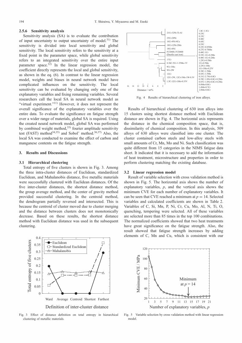
Figure 8 shows correlation coefficient of test dataset forneural network models created by three kinds of activationfunctions and three kinds of normalization methods. Thenormalization method is different for each of the three plots.The horizontal axis represents the dataset number. Overall,the correlation coefficient scattered depending on the testdataset. The method of n1­ReLU, n2­Tanh, n3­Tanh showedrelatively high correlation coefficients, among which n1­ReLU has the smallest variance of the correlation coefficient.Moreover, in the method of n1­ReLU, the training finished atthe smallest epoch number among three activation function.These results agreed with the previous studies. In thenormalization method of n2 and n3, the variables areconverted so as to fit within a certain range, whereas the

0

200

400

600

800

1000

0 200 400 600 800 1000

TrainingTest

Experimental fatigue strength / MPa

Pred

icte

d fa

tigue

stre

ngth

/M

Pa

Fig. 6 Scatter plot of the fatigue strength predicted by the linear regressionmodel.

Table 4 Correlation coefficient and root mean squared error (RMSE) ofmultivariate linear regression model (MR) and artificial neural networkmodel (ANN).

Cross validation error / MPa

Num

ber o

f cou

nts

Umemoto(1995)

78.4 MPa

Mukherjee(2012)

41.2 MPa

Agrawal(2014)

35.7 MPa

Fig. 7 Results of exhaustive search with density of state (ES-DoS) forcross validation error of fatigue strength and comparison with existingmodels.

Prediction of Fatigue Strength in Steels by Linear Regression and Neural Network 195

normalization method of n1 converts variables so that theaverage becomes zero. LeCun et al.24) suggested that if theaverage of the inputs is kept away from zero, the updatingof the weight is biased toward a specific direction and thetraining takes long time. The ReLU function returns zero tothe negative input value, and when combined with thenormalization method of n1, the output of about half units inthe hidden layer becomes zero. According to Glorot et al.,23)

the ReLU function enables sparse representation to invalidatea part of the hidden layer, and suppresses over-fitting bylowering the degree of freedom of the model.

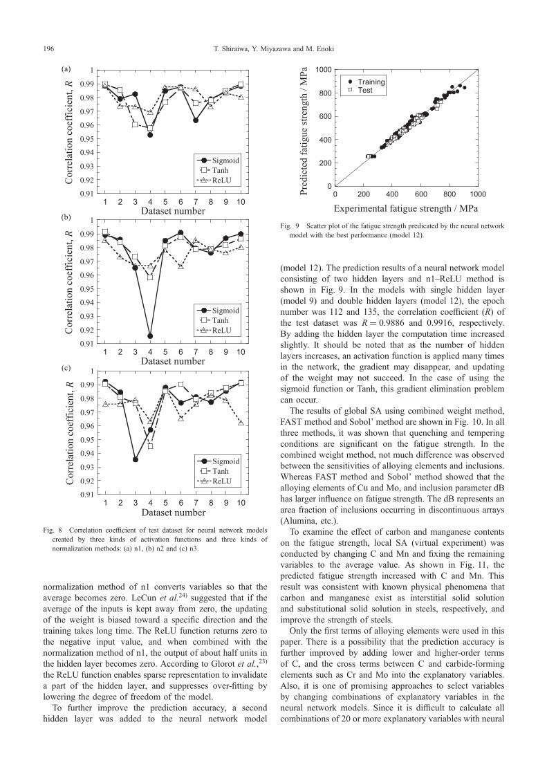
To further improve the prediction accuracy, a secondhidden layer was added to the neural network model

(model 12). The prediction results of a neural network modelconsisting of two hidden layers and n1­ReLU method isshown in Fig. 9. In the models with single hidden layer(model 9) and double hidden layers (model 12), the epochnumber was 112 and 135, the correlation coefficient (R) ofthe test dataset was R = 0.9886 and 0.9916, respectively.By adding the hidden layer the computation time increasedslightly. It should be noted that as the number of hiddenlayers increases, an activation function is applied many timesin the network, the gradient may disappear, and updatingof the weight may not succeed. In the case of using thesigmoid function or Tanh, this gradient elimination problemcan occur.

The results of global SA using combined weight method,FAST method and Sobol’ method are shown in Fig. 10. In allthree methods, it was shown that quenching and temperingconditions are significant on the fatigue strength. In thecombined weight method, not much difference was observedbetween the sensitivities of alloying elements and inclusions.Whereas FAST method and Sobol’ method showed that thealloying elements of Cu and Mo, and inclusion parameter dBhas larger influence on fatigue strength. The dB represents anarea fraction of inclusions occurring in discontinuous arrays(Alumina, etc.).

To examine the effect of carbon and manganese contentson the fatigue strength, local SA (virtual experiment) wasconducted by changing C and Mn and fixing the remainingvariables to the average value. As shown in Fig. 11, thepredicted fatigue strength increased with C and Mn. Thisresult was consistent with known physical phenomena thatcarbon and manganese exist as interstitial solid solutionand substitutional solid solution in steels, respectively, andimprove the strength of steels.

Only the first terms of alloying elements were used in thispaper. There is a possibility that the prediction accuracy isfurther improved by adding lower and higher-order termsof C, and the cross terms between C and carbide-formingelements such as Cr and Mo into the explanatory variables.Also, it is one of promising approaches to select variablesby changing combinations of explanatory variables in theneural network models. Since it is difficult to calculate allcombinations of 20 or more explanatory variables with neural

0.91

0.92

0.93

0.94

0.95

0.96

0.97

0.98

0.99

1

SigmoidTanhReLU

1 2 3 4 5 6 7 8 9 10

0.91

0.92

0.93

0.94

0.95

0.96

0.97

0.98

0.99

1

SigmoidTanhReLU

1 2 3 4 5 6 7 8 9 10

0.91

0.92

0.93

0.94

0.95

0.96

0.97

0.98

0.99

1

SigmoidTanhReLU

1 2 3 4 5 6 7 8 9 10

(a)

(b)

(c)

Dataset number

Cor

rela

tion

coef

ficie

nt, R

Cor

rela

tion

coef

ficie

nt, R

Dataset number

Dataset number

Cor

rela

tion

coef

ficie

nt, R

Fig. 8 Correlation coefficient of test dataset for neural network modelscreated by three kinds of activation functions and three kinds ofnormalization methods: (a) n1, (b) n2 and (c) n3.

0

200

400

600

800

1000

0 200 400 600 800 1000

TrainingTest

Experimental fatigue strength / MPa

Pred

icte

d fa

tigue

stre

ngth

/M

Pa

Fig. 9 Scatter plot of the fatigue strength predicated by the neural networkmodel with the best performance (model 12).

T. Shiraiwa, Y. Miyazawa and M. Enoki196

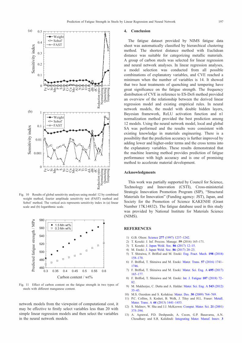
network models from the viewpoint of computational cost, itmay be effective to firstly select variables less than 20 withsimple linear regression models and then select the variablesin the neural network models.

4. Conclusion

The fatigue dataset provided by NIMS fatigue datasheet was automatically classified by hierarchical clusteringmethod. The shortest distance method with Euclideandistance was suitable for categorizing metallic materials.A group of carbon steels was selected for linear regressionand neural network analyses. In linear regression analyses,a model selection was conducted from all possiblecombinations of explanatory variables, and CVE reached aminimum when the number of variables is 14. It showedthat two heat treatments of quenching and tempering havegreat significance on the fatigue strength. The frequencydistribution of CVE in reference to ES-DoS method providedan overview of the relationship between the derived linearregression model and existing empirical rules. In neuralnetwork models, the model with double hidden layers,Bayesian framework, ReLU activation function and n1normalization method provided the best prediction among12 models. Using the neural network model, local and globalSA was performed and the results were consistent withexisting knowledge in materials engineering. There is apossibility that the prediction accuracy is further improved byadding lower and higher-order terms and the cross terms intothe explanatory variables. These results demonstrated thatthe machine learning method provides prediction of fatigueperformance with high accuracy and is one of promisingmethod to accelerate material development.

Acknowledgments

This work was partially supported by Council for Science,Technology and Innovation (CSTI), Cross-ministerialStrategic Innovation Promotion Program (SIP), “StructuralMaterials for Innovation” (Funding agency: JST), Japan, andSociety for the Promotion of Science KAKENHI (GrantNumber 17K14832). The fatigue database used in this studywas provided by National Institute for Materials Science(NIMS).

REFERENCES

1) G.B. Olson: Science 277 (1997) 1237­1242.2) T. Koseki: J. Inf. Process. Manage. 59 (2016) 165­171.3) T. Koseki: J. Japan Weld. Soc. 86 (2017) 12­15.4) M. Enoki: J. Japan Weld. Soc. 86 (2017) 20­23.5) T. Shiraiwa, F. Briffod and M. Enoki: Eng. Fract. Mech. 198 (2018)

158­170.6) F. Briffod, T. Shiraiwa and M. Enoki: Mater. Trans. 57 (2016) 1741­

1746.7) F. Briffod, T. Shiraiwa and M. Enoki: Mater. Sci. Eng. A 695 (2017)

165­177.8) F. Briffod, T. Shiraiwa and M. Enoki: Int. J. Fatigue 107 (2018) 72­

82.9) M. Mukherjee, C. Dutta and A. Haldar: Mater. Sci. Eng. A 543 (2012)

35­43.10) M.S. Ozerdem and S. Kolukisa: Mater. Des. 30 (2009) 764­769.11) P.C. Collins, S. Koduri, B. Welk, J. Tiley and H.L. Fraser: Metall.

Mater. Trans. A 44 (2013) 1441­1453.12) S. Malinov, W. Sha and J.J. McKeown: Comput. Mater. Sci. 21 (2001)

375­394.13) A. Agrawal, P.D. Deshpande, A. Cecen, G.P. Basavarsu, A.N.

Choudhary and S.R. Kalidindi: Integrating Mater. Manuf. Innov. 3

0

0.1

0.2

0.3

0.4

0.5WeightSobol'FAST

Fe C Si Mn P S Ni

Cr

Cu

Mo Al N Ti O dA dB dC

Red

uctio

n ra

tioN

orm

aliz

ing

Que

nchi

ngTe

mpe

ring

0

0.001

0.01

0.1

1WeightSobol'FAST

Fe C Si Mn P S Ni

Cr

Cu

Mo Al N Ti O dA dB dC

Red

uctio

n ra

tioN

orm

aliz

ing

Que

nchi

ngTe

mpe

ring

Sens

itivi

ty in

dex

Sens

itivi

ty in

dex

(a)

(b)

Fig. 10 Results of global sensitivity analyses using model 12 by combinedweight method, fourier amplitude sensitivity test (FAST) method andSobol’ method. The vertical axis represents sensitivity index in (a) linearscale and (b) logarithmic scale.

460

480

500

520

540

560

580

0.3 0.35 0.4 0.45 0.5 0.55 0.6

1.5 Mn wt%0.3 Mn wt%

Carbon content / wt%

Pred

icte

d fa

tigue

stre

ngth

/M

Pa

Fig. 11 Effect of carbon content on the fatigue strength in two types ofsteels with different manganese content.

Prediction of Fatigue Strength in Steels by Linear Regression and Neural Network 197

(2014) 8.14) Fatigue Data Sheet. National Institute for Materials Science (NIMS).

http://smds.nims.go.jp/fatigue, (cited 2018-05-18).15) M. Steinbach, G. Karypis and V. Kumar: KDD Workshop on Text

Mining, (Boston, 2000) pp. 525­526.16) P.C. Mahalanobis: Proceedings of the National Institute of Sciences

(Calcutta), vol. 2, (1936) pp. 49­55.17) S.C. Johnson: Psychometrika 32 (1967) 241­254.18) G.N. Lance and W.T. Williams: Comput. J. 9 (1967) 373­380.19) J.H. Ward: J. Am. Stat. Assoc. 58 (1963) 236­244.20) R.R. Sokal and C.D. Michener: Univ. Kansas Sci. Bull. 28 (1958)

1409­1438.21) C.M. Bishop: Pattern Recognition and Machine Learning, (Springer-

Verlag, New York, 2006) pp. 4­8.22) X. Glorot and Y. Bengio: Proceedings of the Thirteenth International

Conference on Artificial Intelligence and Statistics, Proceedings ofMachine Learning Research, PMLR, (2010) pp. 249­256.

23) X. Glorot, A. Bordes and Y. Bengio: Proceedings of the FourteenthInternational Conference on Artificial Intelligence and Statistics,Proceedings of Machine Learning Research, PMLR, (2011) pp. 315­323.

24) Y. LeCun, Y. Bengio and G. Hinton: Nature 521 (2015) 436.25) Y. LeCun, L. Bottou, G.B. Orr and K.R. Müller: Neural Networks -

Tricks of the Trade, vol. 1524, ed. by G. Orr and K. Müller, (Springer

Verlag, 1998) pp. 5­50.26) J. Sobhani, M. Najimi, A.R. Pourkhorshidi and T. Parhizkar: Constr.

Build. Mater. 24 (2010) 709­718.27) A.A. Suratgar, M.B. Tavakoli and A. Hoseinabadi: World Acad. Sci.

Eng. Technol. 6 (2005) 46­48.28) H. Fujii, D.J.C. Mackay and H.K.D.H. Bhadeshia: ISIJ Int. 36 (1996)

1373­1382.29) H. Fujii and K. Ichikawa: J. Japan Weld. Soc. 70 (2001) 335­339.30) Bayesian methods for neural networks - FAQ. D.J.C. MacKay. http://

www.inference.org.uk/mackay/Bayes_FAQ.html, (cited 2018-05-25).31) M. Koda and T. Honma: Operations Research as a Management

Science Research 55 (2010) 613­621.32) F. Cannavó: Comput. Geosci. 44 (2012) 52­59.33) P. Hajela and Z.P. Szewczyk: Struct. Optim. 8 (1994) 236­241.34) R.I. Cukier, C.M. Fortuin, K.E. Shuler, A.G. Petschek and J.H.

Schaibly: J. Chem. Phys. 59 (1973) 3873­3878.35) R.I. Cukier, J.H. Schaibly and K.E. Shuler: J. Chem. Phys. 63 (1975)

1140­1149.36) I.M. Soboĺ: Math. Comput. Simul. 55 (2001) 271­280.37) I.M. Soboĺ: Prog. Nucl. Energy 24 (1990) 55­61.38) Y. Igarashi, H. Takenaka, Y. Nakanishi-Ohno, M. Uemura, S. Ikeda and

M. Okada: J. Phys. Soc. Jpn. 87 (2018) 044802.39) M. Umemoto: Tetsu-to-Hagané 81 (1995) 157­166.

T. Shiraiwa, Y. Miyazawa and M. Enoki198