Prediction in Multilevel Logistic Regression Sophia Rabe-Hesketh Graduate School of Education & Graduate Group in Biostatistics University of California, Berkeley Institute of Education, University of London Joint work with Anders Skrondal Fall North American Stata Users Group meeting San Francisco, November 2008 . – p.1

Welcome message from author
This document is posted to help you gain knowledge. Please leave a comment to let me know what you think about it! Share it to your friends and learn new things together.
Transcript

Prediction in Multilevel Logistic Regression
Sophia Rabe-Hesketh
Graduate School of Education & Graduate Group in Biostatistics
University of California, Berkeley
Institute of Education, University of London
Joint work with Anders Skrondal
Fall North American Stata Users Group meetingSan Francisco, November 2008
. – p.1

Outline
Application: Abuse of antibiotics in China
Three-level logistic regression model
Prediction of random effects
Empirical Bayes (EB) prediction
Standard errors for EB prediction and approximate CI
Prediction of response probabilities
Conditional response probabilities
Posterior mean response probabilities (different types)
Population-averaged response probabilities
Concluding remarks
. – p.2

Abuse of antibiotics in China
Acute respiratory tract infection (ARI) can lead to pneumonia anddeath if not properly treated
Inappropriate frequent use of antibiotics was common in China in1990’s, leading to drug resistance
In the 1990’s the WHO introduced a program of case managementfor children under 5 with ARI in China
Data collected on 855 children i (level 1) treated by 134 doctors j(level 2) in 36 hospitals k (level 3) in two counties (one of which wasin the WHO program)
Response variable: Whether antibiotics were prescribed when therewere no clinical indications based on medical files
Reference: Min Yang (2001). Multinomial Regression. In Goldstein and Leyland (Eds).Multilevel Modelling of Health Statistics, pages 107-123.
. – p.3

Three-level data structure
Hospital Level 3:36 hospitals k
?
��
��
��
�
@@
@@
@@
@R
Dr. YingDr. YangDr. Wang Level 2:134 doctors j
��
���
AAAAU
Min Shu-Ying
��
���
AAAAU
Chou Chang
��
���
AAAAU
Xiang Jiang Level 1:855 children i
. – p.4

Variables
Response variable yijk
Antibiotics prescribed without clinical indications (1: yes, 0: no)
7 covariates xijk
Patient level i[Age] Age in years (0-4)[Temp] Body temperature, centered at 36◦C[Paymed] Pay for medication (yes=1, no=0)[Selfmed] Self medication (yes=1, no=0)[Wrdiag] Failure to diagnose ARI early (yes=1, no=0)
Doctor level j[DRed] Doctor’s education(6 categories from self-taught to medical school)
Hospital level k[WHO] Hospital in WHO program (yes=1, no=0)
. – p.5

Three-level random intercept logistic regression
Logistic regression with random intercepts for doctors and hospitals
logit[Pr(yijk = 1|xijk, ζ(2)jk , ζ
(3)k )] = x′
ijkβ + ζ(2)jk + ζ
(3)k
Level 3: ζ(3)k |xijk ∼ N(0, ψ(3))
independent across hospitalsψ(3) is residual between-hospital variance
Level 2: ζ(2)jk |xijk, ζ
(3)k ∼ N(0, ψ(2))
independent across doctors, independent of ζ(3)k
ψ(2) is residual between-doctor, within-hospital variance
gllamm command:
gllamm abuse age temp Paymed Selfmed Wrdiag DRed WHO, ///
i(doc hosp) link(logit) family(binom) adapt
. – p.6

Maximum likelihood estimates
No covariates Full model
Parameter Est (SE) Est (SE) (OR)
β0 [Cons] 0.87 (0.14) 1.52 (0.46)β1 [Age] 0.14 (0.07) 1.15β2 [Temp] −0.72 (0.10) 0.49β3 [Paymed] 0.38 (0.30) 1.46β4 [Selfmed] −0.65 (0.21) 0.52β5 [Wrdiag] 1.97 (0.20) 7.18β6 [DRed] −0.20 (0.10) 0.82β7 [WHO] −1.26 (0.32) 0.28
ψ(2) 0.20 0.14ψ(3) 0.36 0.19Log-likelihood −512.14 −415.76
using gllamm with adaptive quadrature
. – p.7
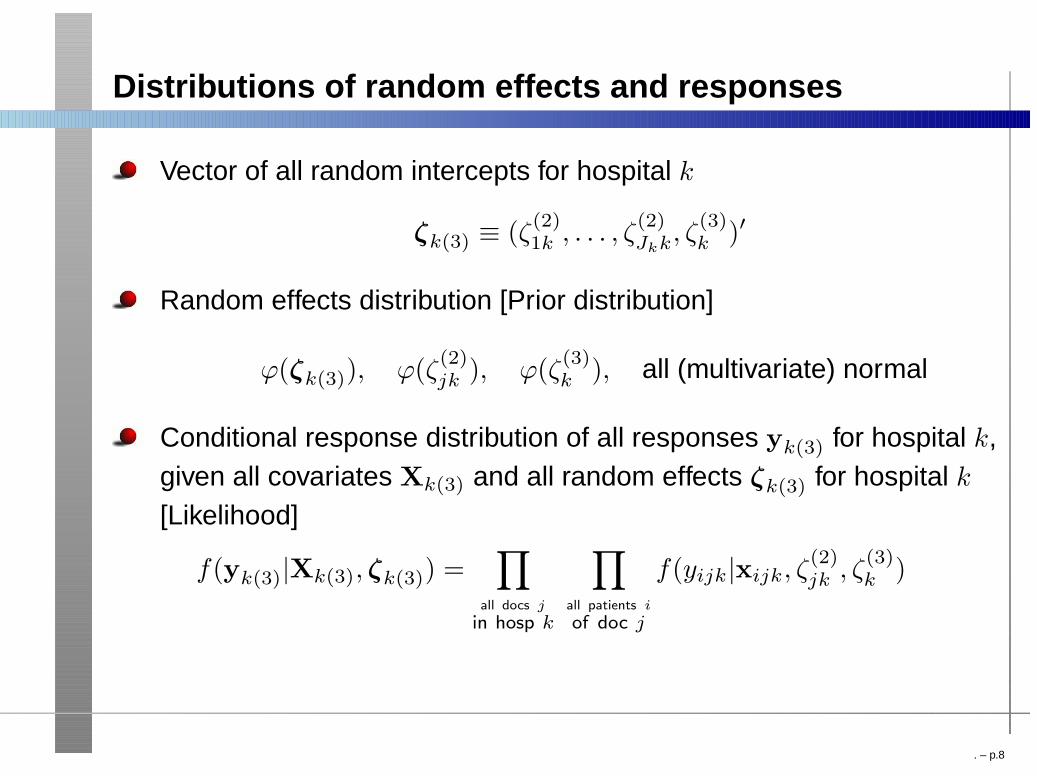
Distributions of random effects and responses
Vector of all random intercepts for hospital k
ζk(3) ≡ (ζ(2)1k , . . . , ζ
(2)Jkk, ζ
(3)k )′
Random effects distribution [Prior distribution]
ϕ(ζk(3)), ϕ(ζ(2)jk ), ϕ(ζ
(3)k ), all (multivariate) normal
Conditional response distribution of all responses yk(3) for hospital k,given all covariates Xk(3) and all random effects ζk(3) for hospital k[Likelihood]
f(yk(3)|Xk(3), ζk(3)) =∏
all docs j
in hosp k
∏
all patients i
of doc j
f(yijk|xijk, ζ(2)jk , ζ
(3)k )
. – p.8

Posterior distribution
Use Bayes theorem to obtain posterior distribution of random effectsgiven the data:
ω(ζk(3)|yk(3),Xk(3)) =ϕ(ζk(3))f(yk(3)|Xk(3), ζk(3))∫
ϕ(ζk(3))f(yk(3)|Xk(3), ζk(3))dζk(3)
∝ ϕ(ζ(3)k )
∏
j
ϕ(ζ(2)jk )
∏
i
f(yijk|xijk, ζ(2)jk , ζ
(3)k )
Denominator, marginal likelihood contribution for hospital k, simplifies∫ϕ(ζ
(3)k )
∏
j
[∫ϕ(ζ
(2)jk )
∏
i
f(yijk|xijk, ζ(2)jk , ζ
(3)k ) dζ
(2)jk
]dζ
(3)k
. – p.9

Empirical Bayes prediction of random effects
Empirical Bayes (EB) prediction is mean of posterior distribution
ζ̃k(3) =
∫ζk(3) ω(ζk(3)|yk(3),Xk(3)) dζk(3)
Standard error of EB is standard deviation of posterior distribution
Using gllapred with the u option
gllapred eb, u
ebm1 contains ζ̃(2)jk
ebs1 contains SE(ζ̃(2)jk )
ebm2 contains ζ̃(3)k
ebs2 contains SE(ζ̃(3)k )
For approximately normal posterior, use Wald-type interval, e.g., forhospital k, 95% CI is ζ̃(3)
k ± 1.96 SE(ζ̃(3)k )
. – p.10
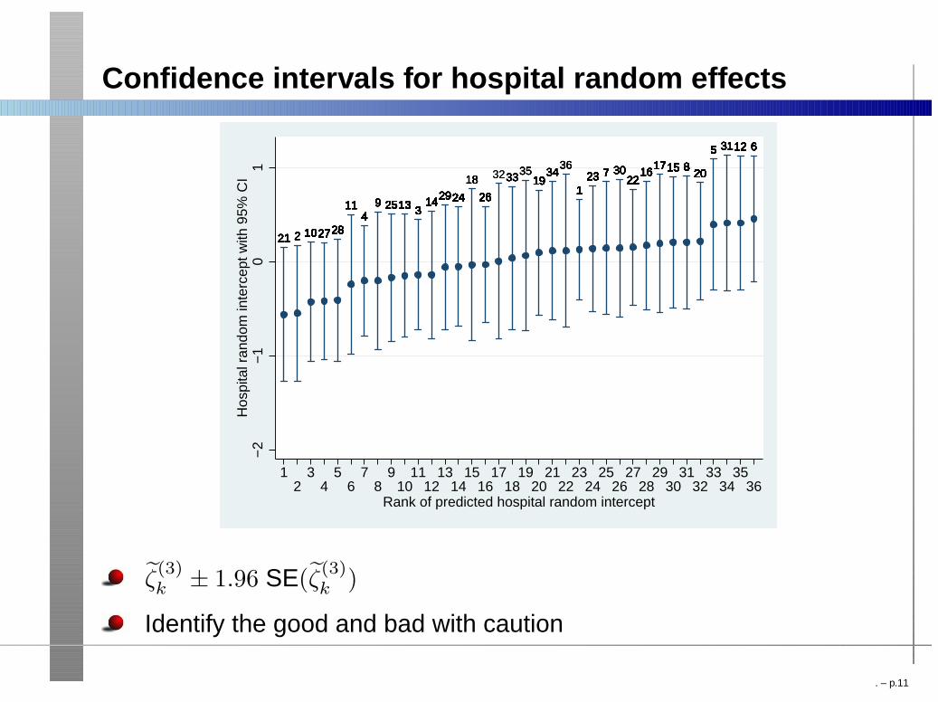
Confidence intervals for hospital random effects
2121212121212121212121212121212121 222222222222222 101010101010101010101010101010101010101010101010101010101010272727272727272727272727272727272727272727272727272727282828282828282828282828282828282828282828282828
11111111111111111111111111444444444444444444444444444444444444444444444
99999999999999 25252525252525252525252525252525252525252525251313131313131313131313131313131313131313131313131313131313 33333333333333333333333333333333333333333333331414141414141414141414141414141414141414141414141414292929292929292929292929292929292929292424242424242424242424242424242424242424242424242424242424242424
181818181818
2626262626262626262626262626262626262626262626262626262626262626262626262626
32323333333333333333353535351919191919191919191919191919191919191919191919191919191919
343434343434343434343436363636
11111111111111111111111111111111111111111111111111111111111111232323232323232323232323232323232323232323232323232323232323 7777777777777777777777 303030303030303030303030
2222222222222222222222222222222222222222222222222222222222222222222222222222222216161616161616161616161616161616161616161616
171717171717171717171717171717171717171717171515151515151515151515151515151515151515151515 88888888888888888888888820202020202020202020202020202020202020202020202020202020202020202020202020
5555555555555555555555555555555 3131313131313131313131313131121212121212121212121212121212121212121212121212 666666666666666666666666666666
−2
−1
01
Hos
pita
l ran
dom
inte
rcep
t with
95%
CI
12
34
56
78
910
1112
1314
1516
1718
1920
2122
2324
2526
2728
2930
3132
3334
3536
Rank of predicted hospital random intercept
ζ̃(3)k ± 1.96 SE(ζ̃
(3)k )
Identify the good and bad with caution
. – p.11

Predicted probability for patientof hypothetical doctor
Predicted conditional probability for hypothetical values x0 of thecovariates and ζ0 of the random intercepts
P̂r(y = 1|x0, ζ0) =exp(x0′β̂ + ζ(2)0 + ζ(3)0)
1 + exp(x0′β̂ + ζ(2)0 + ζ(3)0)
If ζ(2)0 + ζ(3)0 = 0, median of distribution for ζ(2)jk + ζ
(3)k , then
predicted conditional probability is median probability
Analogously for other percentiles
Using gllapred with mu and us() option:
replace age = 2 /* etc.: change covariates to x0*/
generate zeta1 = 0
generate zeta2 = 0
gllapred probc, mu us(zeta)
. – p.12

Predicted probability for new patientof existing doctor in existing hospital
Posterior mean probability for new patient of existing doctor j inhospital k
P̃rjk(y = 1|x0) =
∫P̂r(y = 1|x0, ζk(3))ω(ζk(3)|yk(3),Xk(3)) dζk(3)
Invent additional patient i∗jk with covariate values xi∗jk = x0
Make sure that invented observation does not contribute toposterior ω(ζk(3)|yk(3),Xk(3))
ω(ζk(3)|yk(3),Xk(3)) ∝ ϕ(ζ(3)k )
∏
j
ϕ(ζ(2)jk )
∏
i 6=i∗
f(yijk|xijk, ζ(2)jk , ζ
(3)k )
Cannot simply plug in EB prediction ζ̃k(3) for ζk(3)
P̃rjk(y = 1|x0) 6= P̂r(y = 1|x0, ζk(3) = ζ̃k(3))
. – p.13

Prediction dataset:One new patient per doctor
Data (ignore gaps)
id doc hosp abuse
1 1 1 0
2 1 1 1
. 1 1 .
3 2 2 0
. 2 2 .
4 3 2 1
5 3 2 1
. 3 2 .
Data with invented observations
id doc hosp abuse
1 1 1 0
2 1 1 1
. 1 1 .
3 2 2 0
. 2 2 .
4 3 2 1
5 3 2 1
. 3 2 .Response variable abuse must be missing for invented observations
Use required value of doc
Can invent several patients per doctor
. – p.14
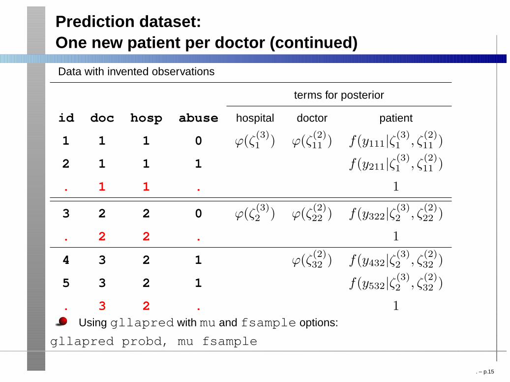
Prediction dataset:One new patient per doctor (continued)
Data with invented observations
terms for posterior
id doc hosp abuse hospital doctor patient
1 1 1 0 ϕ(ζ(3)1 ) ϕ(ζ
(2)11 ) f(y111|ζ
(3)1 , ζ
(2)11 )
2 1 1 1 f(y211|ζ(3)1 , ζ
(2)11 )
. 1 1 . 1
3 2 2 0 ϕ(ζ(3)2 ) ϕ(ζ
(2)22 ) f(y322|ζ
(3)2 , ζ
(2)22 )
. 2 2 . 1
4 3 2 1 ϕ(ζ(2)32 ) f(y432|ζ
(3)2 , ζ
(2)32 )
5 3 2 1 f(y532|ζ(3)2 , ζ
(2)32 )
. 3 2 . 1Using gllapred with mu and fsample options:
gllapred probd, mu fsample
. – p.15
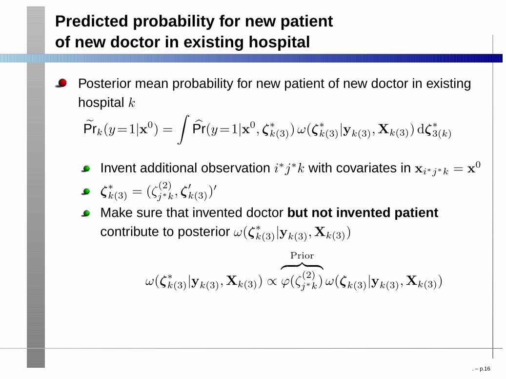
Predicted probability for new patientof new doctor in existing hospital
Posterior mean probability for new patient of new doctor in existinghospital k
P̃rk(y=1|x0) =
∫P̂r(y=1|x0, ζ∗
k(3))ω(ζ∗k(3)|yk(3),Xk(3)) dζ∗
3(k)
Invent additional observation i∗j∗k with covariates in xi∗j∗k = x0
ζ∗k(3) = (ζ
(2)j∗k, ζ
′k(3))
′
Make sure that invented doctor but not invented patientcontribute to posterior ω(ζ∗
k(3)|yk(3),Xk(3))
ω(ζ∗k(3)|yk(3),Xk(3)) ∝
Prior︷ ︸︸ ︷ϕ(ζ
(2)j∗k)ω(ζk(3)|yk(3),Xk(3))
. – p.16

Prediction dataset:One new doctor and patient per hospital
Data (ignore gaps)
id doc hosp abuse
1 1 1 0
2 1 1 1
. 1 1 .
3 2 2 0
4 3 2 1
5 3 2 1
. 3 2 .
Data with invented observations
id doc hosp abuse
1 1 1 0
2 1 1 1
. 0 1 .
3 2 2 0
4 3 2 1
5 3 2 1
. 0 2 .
Response variable abuse must be missing for invented observations
Use unique (for that hospital) value of doc
Can invent several new docs which can all have the same value of doc
. – p.17

Prediction dataset:One new doctor and patient per hospital (continued)
Data with invented observations
terms for posterior
id doc hosp abuse hospital doctor patient
1 1 1 0 ϕ(ζ(3)1 ) ϕ(ζ
(2)11 ) f(y111|ζ
(3)1 , ζ
(2)11 )
2 1 1 1 f(y211|ζ(3)1 , ζ
(2)11 )
. 0 1 . ϕ(ζ(2)01 ) 1
3 2 2 0 ϕ(ζ(3)2 ) ϕ(ζ
(2)22 ) f(y322|ζ
(3)2 , ζ
(2)22 )
4 3 2 1 ϕ(ζ(2)32 ) f(y432|ζ
(3)2 , ζ
(2)32 )
5 3 2 1 f(y532|ζ(3)2 , ζ
(2)32 )
. 0 2 . ϕ(ζ(2)02 ) 1
Using gllapred with mu and fsample options:
gllapred probh, mu fsample
. – p.18

Example: Predicted probability for new patientof new doctor in existing hospital
.2.4
.6.8
Pre
dict
ed p
oste
rior
mea
n pr
obab
ility
1 2 3 4 5 6Doctor’s qualification
Each curve represents a hospitalFor each hospital: 6 new doctors with [DRed] = 1, 2, 3, 4, 5, 6
For each doctor: 1 new patient with [Age] = 2, [Temp] = 1 (37◦C), [Paymed] = 0,
[Selfmed] = 0, [Wrdiag] = 0
. – p.19

Example: Predicted probability for new patientof existing doctor in existing hospital
.2.4
.6.8
.2.4
.6.8
.2.4
.6.8
1 2 3 4 5 6 1 2 3 4 5 6 1 2 3 4 5 6 1 2 3 4 5 6
1 3 4 6
8 10 13 19
20 22 25 28
Pre
dict
ed p
oste
rior
mea
n pr
obab
ility
Doctor’s qualificationGraphs by hosp
12 of the hospitals, with curves as in previous slideDots represent doctors with [DRed] as observedFor each doctor: predicted probability for 1 new patient with [Age] = 2, [Temp] = 1,
[Paymed] = 0, [Selfmed] = 0, [Wrdiag] = 0
. – p.20

Predicted probability for new patientof new doctor in new hospital
Population-averaged or marginal probability:
Pr(y=1|x0) =
∫P̂r(y = 1|x0, ζ
(2)jk , ζ
(3)k )ϕ(ζ
(2)jk ), ϕ(ζ
(3)k ) dζ
(2)jk dζ
(3)k
Cannot plug in means of random intercepts
Pr(y = 1|x0) 6= P̂r(y = 1|x0, ζ(2)jk = 0, ζ
(3)k = 0)
mean 6= median
Using gllapred with the mu and marg options:
gllapred prob, mu marg fsample
Confidence interval, by sampling parameters from the estimatedasymptotic sampling distribution of their estimates
ci_marg_mu lower upper, level(95) dots
. – p.21

Illustration Cluster-specific:versus population averaged probability
0 20 40 60 80 100
0.0
0.2
0.4
0.6
0.8
1.0
x
Pro
babi
lity
cluster-specific (random sample)medianpopulation averaged
. – p.22

Illustration Cluster-specific:versus population averaged probability
0 20 40 60 80 100
0.0
0.2
0.4
0.6
0.8
1.0
x
Pro
babi
lity
cluster-specific (random sample)medianpopulation averaged
. – p.22
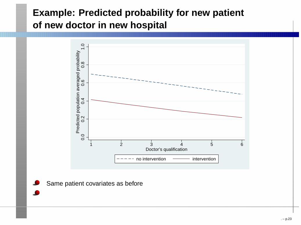
Example: Predicted probability for new patientof new doctor in new hospital
0.0
0.2
0.4
0.6
0.8
1.0
Pre
dict
ed p
opul
atio
n av
erag
ed p
roba
bilit
y
1 2 3 4 5 6Doctor’s qualification
no intervention intervention
Same patient covariates as before
Confidence bands represent parameter uncertainty
. – p.23

Example: Predicted probability for new patientof new doctor in new hospital
0.0
0.2
0.4
0.6
0.8
1.0
Pop
ulat
ion
aver
aged
pro
babi
lity
with
95%
CI
1 2 3 4 5 6Doctor’s qualification
no intervention intervention
Same patient covariates as before
Confidence bands represent parameter uncertainty
. – p.23

Concluding remarks
Discussed:
Empirical Bayes (EB) prediction of random effects and CI usinggllapred, ignoring parameter uncertainty
Prediction of different kinds of probabilities using gllapred aftercareful preparation of prediction dataset
Simulation-based CI for predicted marginal probabilities usingnew command ci_marg_mu
Methods work for any GLLAMM model, including random-coefficientmodels and models for ordinal, nominal or count data
Assumed normal random effects distribution
EB predictions not robust to misspecification of distribution
Could use nonparametric maximum likelihood in gllamm,followed by same gllapred and ci_marg_mu commands
. – p.24

References
Rabe-Hesketh, S. and Skrondal, A. (2008).Multilevel and Longitudinal Modeling Using Stata(2nd Edition). College Station, TX: Stata Press.
Skrondal, A. and Rabe-Hesketh, S. (2009). Prediction in multilevelgeneralized linear models. Journal of the Royal Statistical Society,Series A, in press.
Rabe-Hesketh, S., Skrondal, A. and Pickles, A. (2005). Maximumlikelihood estimation of limited and discrete dependent variablemodels with nested random effects. Journal of Econometrics 128,301-323.
. – p.25
Related Documents


![[ME] Multilevel Mixed Effects - Stata · Title me — Introduction to multilevel mixed-effects models DescriptionQuick startSyntaxRemarks and examples AcknowledgmentsReferencesAlso](https://static.cupdf.com/doc/110x72/5fda116a20c50d3a9c01a419/me-multilevel-mixed-effects-stata-title-me-a-introduction-to-multilevel-mixed-effects.jpg)
![[ME] Multilevel Mixed Effectspublic.econ.duke.edu/stata/Stata-13-Documentation/me.pdf · The software described in this manual is furnished under a license agreement or nondisclosure](https://static.cupdf.com/doc/110x72/60285b4ac09acb231403817b/me-multilevel-mixed-the-software-described-in-this-manual-is-furnished-under-a.jpg)