0 Predicting the Path of Technological Innovation: SAW Versus Moore, Bass, Gompertz, and Kryder Ashish Sood, Gareth M. James, Gerard J. Tellis, and Ji Zhu* Marketing Science Author note * Ashish Sood ([email protected]) is Assistant Professor of Marketing, Goizueta School of Business, Emory University. Address: 1300 Clifton Rd NE, Atlanta, GA 30322; Tel: +1.404.727.4226, Fax: +1.404-727-3552 Web: www.ashishsood.net. Gareth James ([email protected]) is Professor of Statistics, Marshall School of Business, University of Southern California Address: P.O. Box 90089-0809, Los Angeles, California, USA; Tel: +1.213.740.9696, fax: +1.213.740.7313 Web: www.gtellis.net. Gerard J. Tellis ([email protected]) is Neely Chair of American Enterprise, Director of the Center for Global Innovation and Professor of Marketing at the Marshall School of Business, University of Southern California. Address: P.O. Box 90089-1421, Los Angeles, California, USA. Tel: +1.213.740.5031, fax: +1.213.740.7828. Ji Zhu ([email protected]) is Associate Professor of Statistics, Department of Statistics, University of Michigan, Ann Arbor. Address: 455 West Hall, 1085 South University Ave., Ann Arbor, MI 48109. Tel: +1.734.936.2577, Fax: +1.734.763. 4674. The study benefited from Dean's Research Grant Award, Emory University, a gift of Don Murray to the USC Marshall Center for Global Innovation, and from the comments of participants at the ISBM Academic Conference, AMA Winter Conference, Marketing Science, and BPS/TIM/ENT Panel Symposium at the Annual Meeting of the Academy of Management.

Welcome message from author
This document is posted to help you gain knowledge. Please leave a comment to let me know what you think about it! Share it to your friends and learn new things together.
Transcript
0
Predicting the Path of Technological Innovation: SAW Versus Moore, Bass, Gompertz, and Kryder
Ashish Sood, Gareth M. James, Gerard J. Tellis, and Ji Zhu*
Marketing Science
Author note
* Ashish Sood ([email protected]) is Assistant Professor of Marketing, Goizueta School
of Business, Emory University. Address: 1300 Clifton Rd NE, Atlanta, GA 30322; Tel:
+1.404.727.4226, Fax: +1.404-727-3552 Web: www.ashishsood.net.
Gareth James ([email protected]) is Professor of Statistics, Marshall School of Business,
University of Southern California Address: P.O. Box 90089-0809, Los Angeles, California,
USA; Tel: +1.213.740.9696, fax: +1.213.740.7313 Web: www.gtellis.net.
Gerard J. Tellis ([email protected]) is Neely Chair of American Enterprise, Director of the Center
for Global Innovation and Professor of Marketing at the Marshall School of Business, University
of Southern California. Address: P.O. Box 90089-1421, Los Angeles, California, USA. Tel:
+1.213.740.5031, fax: +1.213.740.7828.
Ji Zhu ([email protected]) is Associate Professor of Statistics, Department of Statistics,
University of Michigan, Ann Arbor. Address: 455 West Hall, 1085 South University Ave., Ann
Arbor, MI 48109. Tel: +1.734.936.2577, Fax: +1.734.763. 4674.
The study benefited from Dean's Research Grant Award, Emory University, a gift of Don
Murray to the USC Marshall Center for Global Innovation, and from the comments of
participants at the ISBM Academic Conference, AMA Winter Conference, Marketing Science,
and BPS/TIM/ENT Panel Symposium at the Annual Meeting of the Academy of Management.
1
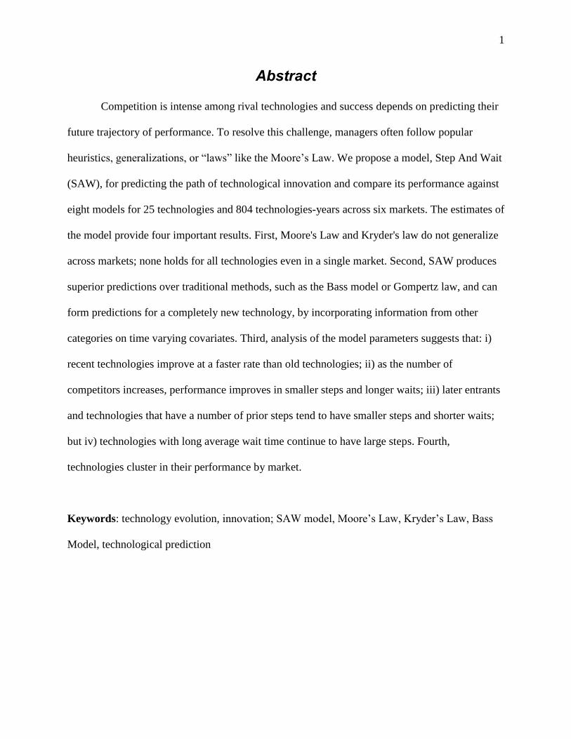
Abstract
Competition is intense among rival technologies and success depends on predicting their
future trajectory of performance. To resolve this challenge, managers often follow popular
heuristics, generalizations, or “laws” like the Moore’s Law. We propose a model, Step And Wait
(SAW), for predicting the path of technological innovation and compare its performance against
eight models for 25 technologies and 804 technologies-years across six markets. The estimates of
the model provide four important results. First, Moore's Law and Kryder's law do not generalize
across markets; none holds for all technologies even in a single market. Second, SAW produces
superior predictions over traditional methods, such as the Bass model or Gompertz law, and can
form predictions for a completely new technology, by incorporating information from other
categories on time varying covariates. Third, analysis of the model parameters suggests that: i)
recent technologies improve at a faster rate than old technologies; ii) as the number of
competitors increases, performance improves in smaller steps and longer waits; iii) later entrants
and technologies that have a number of prior steps tend to have smaller steps and shorter waits;
but iv) technologies with long average wait time continue to have large steps. Fourth,
technologies cluster in their performance by market.
Keywords: technology evolution, innovation; SAW model, Moore’s Law, Kryder’s Law, Bass
Model, technological prediction
2
Introduction Competition is intense among rival technologies in many industries. For example, which
is the technology for auto-batteries of the future: lead-acid, nickel cadmium, fuel-cell, or lithium
ion? Similarly, which is the technology for display monitors of the future: LCD (liquid crystal
diode), LED (light emitting diode), Plasma, or OLED (organic light emitting diode)? How
should firms choose among competing technologies? This is probably the pre-eminent challenge
facing managers of firms in technology driven markets (Hauser, Tellis and Griffin 2007; Tellis
2008).
To resolve this challenge and predict technology change, managers often follow popular
heuristics, generalizations, or “laws”. Examples of such generalizations are Moore’s Law,
Kryder’s Law, and the logistic model. Some of these laws gain wide acceptance and begin to
serve as self-fulfilling prophecies. For example, Moore (2003) suggests that Moore’s Law drove
semiconductor firms to focus enormous energy and make large investments in a race to achieve
performance predicted by the law ahead of their competitors.
However, most generalizations and long range predictions fail, offering little help in
managerial decision making for at least four reasons (Armstrong 2005; Balachandra 1980;
Makridakis et al 1982; Tashman 2000). First, heuristics or laws may be based on cursory
observations of short term patterns instead of on a scientific study of long-term data (e.g. by
Moore 1965). Such heuristics or laws may not survive careful testing. Second, the law itself may
be vague in specification with many contradictory versions. For example, at least two versions of
Moore’s law are popular (performance doubling every year and doubling every 18 months). The
implications of this uncertainty can be substantial. For example, a technology that doubles its
performance every 18 months improves to 100 times its initial performance over 10 years
whereas a technology that doubles every year improves to more than 1000 times its initial
3
performance in the same period. Third, the popularity of a law may encourage indiscriminate
extension to many fields, technologies, and industries. For example, Moore’s law has been
claimed to apply to several metrics of technology performance including the size, cost, density
and speed of components in the semiconductor industry and many other technologies besides
semiconductors like biotechnology, nanotechnology, and genomics (Edwards 2008; Wolff 2004).
In fact, Moore (2003, p. 1) suggests that the law has come to refer to “almost anything related to
the semiconductor industry that when plotted on a semi-log paper approximates a straight line”.
Note that without the exact specification of the slope of the straight line, the law is intrinsically
flexible, and susceptible to hindsight bias. Fourth, prior research is inconclusive on whether the
path of technology evolution is smooth or irregular, suggesting that a data driven approach is
better for prediction than dependence on generalized heuristics. All four reasons suggest the need
for a better model for predicting the path of technology evolution. The current research addresses
these limitations in the literature on technology evolution and addresses these research questions:
How valid are the traditional laws and models for describing technology evolution?
Which model can best predict the path of technological innovation?
What are the key drivers of technology evolution?
To address these questions, we propose a new model, called Step and Wait (SAW) and
test it against extant models on 25 technologies and 804 technologies-years across six markets
over several decades. We make four contributions to current literature. First, we propose a model
to predict the evolution of technological performance that provides better predictions than
traditional models. Such prediction allows both marketing and technology managers to identify
dimensions on which to focus their new product design efforts. Second, the proposed model
allows for predicting the path of an entirely new technology based on the similarity of its
4
characteristics to those of prior technologies. Third, the exercise enables us to test the validity
and generalizability of some popular “laws” about technology evolution. Fourth, we identify key
drivers of technology evolution.
The next five sections present the theory, hypotheses, models, method, and results. The
last section discusses the findings, implications, and limitations of the research.
Theory of Technology Evolution Technology evolution is the improvement in the performance of a technology over time.
We are interested in a better understanding of the path of such improvement. Prior literature has
debated the shape of the path (whether smooth or discontinuous) and the drivers of the path
(explanatory variables that influence its course). We cover both of these topics next.
Shape of Path Prior literature suggests both smooth change through incremental improvements
occurring frequently (Basalla 1988; Dosi 1982) and non-smooth change through relatively stable
periods of smooth change punctuated with discontinuous steps of big changes (D’Aveni 1994;
Eldredge and Gould 1972; Tushman and Anderson 1986).
Proponents of smooth and incremental technological change (Bassalla 1988) argue that
technology evolution is a process of continual improvement in performance of a technology
through novel recombination and synthesis of existing technologies (Henderson and Clark 1990).
These researchers suggest that changes in technology performance are a result of changes in a
number of domains including beliefs, values, culture, technology, operating routines,
organizational structure, resources, and core competencies (Gersick 1991; Tushman and
Romanelli 1985; Wollin 1999). Invention is a social process that rests on the accumulation of
many minor improvements not the heroic efforts of a few geniuses (Basalla 1988; Dosi 1982).
5
Proponents of irregular change suggest that technologies improve through eras of smooth
change punctuated by discontinuous shifts (Adner 2002; Eldredge and Gould 1972; Tushman
and Anderson 1986). Products that draw upon fundamentally new technologies enter an industry,
and create ferment till the emergence of dominant designs (Nelson and Winter 1977; Utterback
and Abernathy 1975). After a dominant design is established, firms focus more on process
innovations than on product innovations (Henderson and Clark 1990). Jumps in product
performance could occur both from product and process innovation related to the focal
technology. Tushman and Anderson (1986) explain the discontinuous nature of technological
change through two types of change – competence enhancing and competence destroying.
Levinthal (1998) extends the concept of natural speciation (Eldredge and Gould 1972) to
technology speciation. Substantial improvements in performance occur because a shift of a
technology from one domain to another alters the relative preference for attributes, demands
different price/performance ratio for older attributes, and often releases substantially higher
resources for R&D (Levinthal 1998). This shift may be due to 1) changes in problem-solving
heuristics, 2) fusion with other domains, and 3) other technological, social, or economic aspects.
Such shifts provide access to new customers, resources, and performance metrics (Adner 2002).
As a result, the technology exhibits sharp steps in performance.
In summary, even though debate in prior research is inconclusive on whether technology
evolution is smooth or irregular, the question remains important to managers. Thus, good
forecasting capabilities may spell the difference between success and failure in the market.

6
Drivers of Path of Technological Change Our review of the theory in this area suggests four covariates that could drive the path of
technological change. We discuss the role of each of these covariates next.1
Year of Introduction The covariate “Year of Introduction” reflects the newness of the technology. We
hypothesize that new technologies improve in larger and more frequent steps than old
technologies due to the improvement in the supporting environment for innovation in recent
years. In particular, improvements in supporting environment are characterized by 1) higher total
R&D expenditures, 2) more researchers devoted to technology research, 3) use of better tools, 4)
better laboratories, 5) better communication of research, 6) more countries focused on research.
In addition, the pace of improvement in new technologies may occur more frequently and
in larger steps than old technologies for three reasons: First, after a period of rapid improvement
in performance, old technologies may reach a period of maturity (Foster 1986; Brown 1992;
Chandy and Tellis 2000; Sood and Tellis 2011). Foster suggests that maturation may be an innate
feature of each technology. Sahal (1981) proposes that the maturity occurs because of limits of
scale or system complexity. Fleming (2001) suggests that old technologies reach ‘recombinant
exhaustion’ and improvements become smaller. Golder and Tellis 2004 suggest that maturation
can result from abandonment following a cascade. Second, newer technologies attract the interest
of firms. Market power acquired from successful innovation in the old technologies spur greater
inventive activity in new technologies. They at one and the same time appear mysterious yet
promise huge benefits. As such, they attract. Third, new technologies also introduce new
performance dimensions unrelated to those offered by old technologies. For example, prior to the
1 Other factors (e.g. market size, technological sophistication) may also affect the evolution, but have not been
included in the analysis due to the lack of reliable data on these variables. We thank the anonymous reviewer for
suggesting these.
7
advent of LCD monitors, firms making CRT monitors competed mainly on higher screen
resolution. LCD monitors promised compactness as a new performance dimension. Old
technologies strive to compete as customer’s demand for these dimensions increases. This slows
performance improvements on the existing dimension. Thus, we hypothesize:
H1: Performance of more recent technologies increases in 1) larger steps and 2) more
frequent steps (shorter wait times).
Order of Entry After controlling for the basic effect of calendar time, the order of entry of a technology
in a particular market could affect its improvement. We need to emphasize that the time effect
probably holds for large time spans such as decades. The order of entry works for small time
spans such as a few years within a market, within which one technology follows another pretty
rapidly. We identify two rival theories: preferential attraction versus pre-commitment.
The preferential attraction theory holds that the earlier technology gets the most (or better
and initially all) of the limited set of resources (dollars, locations, and researchers) than those
that follow. Risk aversion of investors and researchers prevents them from investing in new
technologies. Prior literature also suggests that pioneers outperform later entrants (Lambkin
1988; Urban et al 1986). If this line of reasoning is valid, the earlier technology will have larger
and more frequent improvements in performance than later technologies within the same market.
The above argument leads to the following hypothesis:
H2a: Technology entering earlier improve with 1) larger steps and 2) more frequent steps
(shorter wait times) than later technologies within the same market.
The pre-commitment argument suggests that the earlier technology enters in an
environment with less information about potential markets, dimensions of performance, and
available resources, than the technology that enters later. Thus, the earlier technology pre-
commits to an evolutionary path that may not be the most efficient or effective. The later
technology enters in an environment with greater information about markets, technologies, and
8
resources, and chooses a more efficient and productive evolutionary path (Golder and Tellis
1993). The glamour of the “new” may also result in suppliers switching resources from the old to
the new. Thus, technologies entering later to a market will have more resources and more
researchers working on it than the old technology. This will result in more frequent but smaller
steps in performance . The above argument leads to the following rival hypothesis:
H2b: Technology entering later improve with 1) smaller steps and 2) more frequent steps
(shorter wait times) than earlier technologies to a market.
Number of Competing Technologies Controlling for the effects above, how does improvement relate to the number of
competing technologies? We propose two rival theories: competition for limited resources or
competition spurring breakthroughs.
The limitation of resources theory is that in any market the amount of dollars,
researchers, and labs is relatively fixed in the immediate short term. Thus as the number of
competing technologies increases, each gets less. This division of resources results in less
frequent breakthroughs and therefore less frequent increases in performance. More competition
leads firms to become more risk averse and focus on cost management instead of risky and costly
product improvement. Firms generally achieve these objectives by prioritizing process
innovation over product innovation (Scherer and Ross 1990). Thus, as the number of competitors
increases, improvements in performance are slower.
The rival theory is of competition spurring breakthroughs. This phenomenon could occur
for several reasons. First, each technology is supported by a unique set of researchers with their
own egos, training, reputation, and emotional attachment. As the number of competing
technologies increases, their supporters work harder to promote their own technologies and
create improvements in performance. It is also possible that more firms enter a market because a)

9
there is demand or b) because they think it is relatively easy to improve existing products
(technologies). In other words, if b) is true there are more entrants because technological
progress is likely to be fast2. As a result, the number of improvements in performance increases
with the number of competition technologies in a market. Second, Rosenberg (1969) refers to a
phenomenon of ‘compulsive sequence’ where a breakthrough in one area typically generates new
technical problems creating imbalances that require further innovative effort to realize fully the
benefits of the initial breakthrough. For example, the development of high speed steel improved
cutting tools, and stimulated the development of sturdier and more adaptable machines to drive
them (Rosenberg 1969). Third, new technologies may set up additional opportunities in new
niches even for old technologies. Fourth, prior research suggests that a firm’s returns from
innovation at the margin are larger in an oligopolistic versus a monopolistic environment
(Fellner 1961; Arrow 1962; Scherer 1967). Thus, more competition generates more funds to
support innovation and faster product improvements. All these reasons suggest that an increase
in the number of competitors will increase the number of improvements in technology
performance. Thus, we can propose the following rival hypotheses:
H3a: As the number of competitors increases, performance of technologies increases in 1)
smaller steps and 2) longer wait times.
H3b: As the number of competitors increases, performance of technologies increases in 1)
larger steps and 2) shorter wait times.
Technology Characteristics We include two covariates to capture technology characteristics – number of prior steps
and average prior wait time. Together the two covariates capture unique patterns of technological
improvement for a technology within its unique technological paradigm (Nelson and Winter
1982; Dosi 1982). A technological paradigm is the common platform on which scientists and
technologists agree to do research and explain the speed and pattern of technological
2 We thank the anonymous reviewer for suggesting this possibility.

10
advancement. For example, for the past 30 years, firms in the magnetic storage industry pursued
higher areal density as a goal to solve design problems and achieve higher productivity. This
common understanding, led firms to race to introduce improvements in areal density ahead of
other firms. In this urgency, firms may not delay investments in R&D and frequently introduce
products with improvements.
In technologies where such a paradigm emerges, a technology evolves with a large
number of steps. However, these steps are small and frequent. Firms take advantage of inter-
dependencies with components and advancements in other fields. For example, improvements in
areal density of magnetic storage have partly been driven by advancements in other related
disciplines like semiconductor, fiber-optic, and micro-electronics.
In the absence of a dominant technological paradigm, firms’ efforts scatter in diverse
directions. R&D efforts may be targeted towards improvements on diverse performance metrics
leading to little synergy across firms’ efforts and fewer steps. Also, competing firms within an
industry may wait to introduce products to optimize commercialization costs. As a result, there
are few steps with long wait times. Longer average wait times also provide firms more time to
develop better products. This results in technological progress with large step sizes and long wait
times. Thus, the technological paradigm theory suggests the following two hypotheses:
H4: Technologies with a large number of prior steps have 1) small current step and 2)
shorter current wait time.
H5: Technologies with long average prior wait times have 1) large current step and 2) long
current wait time.
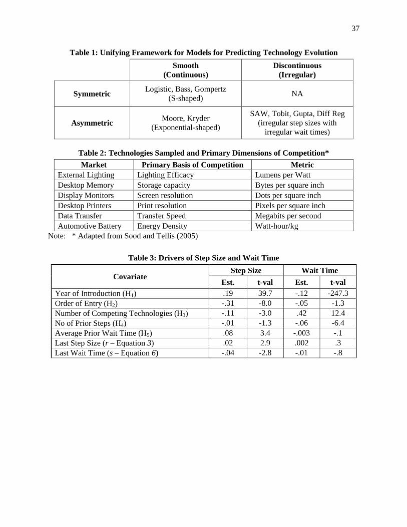
Models This section describes eight models in the literature that have been or could be used to
predict technological change and one model (SAW) that we propose specifically for this purpose
(see Table 1). One of the models is an exponential function used to fit both Moore’s Law and

11
Kryder’s Law (see Figure A1a in Appendix A). Three more models are the most popular
methods used in prior literature to test an S-shaped curve: the Bass, Logistic, and Gompertz
models (see Figure A1b in Appendix A). All four models are smooth and do not allow the use of
explanatory variables in their popular formulation. We propose modified versions of these four
models which do include explanatory variables to allow fair comparison with SAW (see
Appendix B). The next two models are discontinuous and allow the use of explanatory variables:
the Gupta model for buyer interpurchase behavior and the Tobit-II model used to model
technology evolution (see Figure A1c in Appendix A). Appendix B provides details on the
models and explains how these models predict for holdout periods and technologies. We also
include two simple models for comparison – the Naïve method that does not use covariates and
the DiffReg approach that implements a linear regression with covariates.
Moore’s Law (Exponential Model) First proposed by Intel co-founder Gordon E. Moore, the law suggests that the density of
integrated circuits doubles in performance every year (Moore 1965). Thus, Moore’s law specifies
an exponential relationship between technology performance and time (see Figure A1a in
Appendix A and (14) in Appendix B). Later Moore revised the law to a doubling in performance
every two years (Moore 1975). Subsequently, Moore claimed that the performance of “almost
anything related to the semiconductor industry” (Moore 1997 SPIE speech) improves at
exponential rates across a number of measures like size, cost (or experience), density and speed
of components. Over the last few decades, many technologies like microprocessors and DRAMs
seem to have followed a revised Moore’s law that suggests doubling every 18 months (Mollick
2006; Schaller 1997). Researchers suggest that the law also describes technology evolution for
many other technologies besides semiconductors like biotechnology, nanotechnology, and
genomics (Edwards 2008; Wolff 2004). If so, the designation of a “law” would be valid.
12
Kryder’s law (Exponential Model) First proposed by Seagate’s Chief Technology Officer Mark Kryder, the law suggests
that the density of information on hard drives, also known as areal density, “increased by a
factor of 1,000 every 10.5 years since introduction of these technologies” (Walter 2005, pp 32).
This rate is equivalent to a doubling of performance every 13 months (Shacklett 2008).
Grochowski (1998) suggests that the areal density has increased at a compound annual growth
rate of 60%. In effect, both Moore’s Law and Kryder’s Law specify the same exponential form
with differing parameters on time (Figure A1a in Appendix A and (14) in Appendix B).
Logistic Model One theory of the evolution of technology is the theory of S-curves (Foster 1986). This
theory suggests that a plot of maximum performance of a technology over time follows an S-
shaped curve (see Figure A1b in Appendix A and (16) in Appendix B). The S-curve results from
changes in performance on one dimension over the life of the technology. In the early years after
introduction, the performance improves slowly because of technical problems with mastering the
new technology. Once initial bottlenecks have been resolved, the performance improves rapidly
as the technology draws researchers and resources. Eventually the rate of improvement declines
either because the technology reaches limits of scale or size (Sahal 1981) or firms start investing
in alternate technologies (Abernathy and Utterback 1978).
Bass Model
Some researchers examining the diffusion of new products suggest a demand side
explanation of the phenomenon of technology evolution (Adner 2002; Bass 1969; Rogers 1962;
Young and Ord 1989; Young 1993). These researchers suggest that consumers adopt a new
product based on spontaneous innovation driven by word-of-mouth diffusion. This process
carves a typical S-shape of sales of a new product (Sood, James and Tellis 2009) (see Figure A1b
13
in Appendix A and (18) in Appendix B). The demand for the new product drives the evolution of
a new technology, on which the new product is based, and also follows an S-curve.
Gompertz' Model Gompertz’ Law was first proposed by British actuary Benjamin Gompertz for use in
demographic studies and suggests that the rate of human mortality increases exponentially with
age (Gompertz 1825). In the current context, Gompertz’ Law states that maturity and exit of old
technologies pave the way for the new technologies and drive technology evolution (Young and
Ord 1989). The rate of change in the performance of a technology increases at an exponential
rate tracing a sigmoid double exponential S-shaped path over the life of the technology from
introduction till maturity (see Figure A1b in Appendix A and (21) in Appendix B). Gompertz’
Law has been used extensively in prior literature to describe technology evolution because it also
produces S-shaped curves that describe different phases of the evolution –acceleration, inflexion,
and deceleration of growth over time (Martino 2003; Meade and Islam 1995; 1998; 2006; Young
and Ord 1989). The different S-shaped curves have different implications in symmetry around
the relative location of the inflection point. These differences may influence the power of these
laws to predict technology evolution.
Gupta Model
The model of Gupta (1988) is a well-known and popular approach for modeling
consumer purchase decisions. This model consists of three separate stages: brand choice (for
modeling the probability of purchasing a particular brand), interpurchase time (for modeling time
until purchase) and purchase quantity (for modeling the amount of goods purchased). We use
two stages of this model, interpurchase time and quantity to model wait time and size of step,
respectively. This model provides a natural approach for predicting the discontinuous nature of
technology evolution (see Figure A1c in Appendix A and (23) and (24) in Appendix B).

14
Tobit II Model
The Tobit models the evolution of technologies as a series of step-functions with random
improvements over irregular periods of time (see Figure A1c in Appendix A and (25) and (26) in
Appendix B). The model includes a latent variable that represents the probability of a step as a
function of explanatory variables.
Simple Models – Naïve and Diff Reg We also include two simple alternatives. The first method, Naïve, models technology
curves as constant in the holdout period. In other words, we assume that the curve for each
technology is horizontal i.e. if our last observation in the estimation sample is , we predict for
the entire holdout period. The second method, Diff Reg, performs a single linear regression on
all technologies simultaneously using a technology specific indicator variable and the covariates
from the previous section as the independent variables. The indicator variable is modeled as a
random effect. The change in (log) technology performance between two successive periods is
used as the dependent variable. So for example, if a technology remained constant between two
periods, we set for the response. After fitting the linear regression model, we use the
covariates of a technology to predict its change in each time period and hence, the entire
trajectory.
The SAW Model We propose a new approach which models technologies as exhibiting periods of constant
performance followed by discontinuous steps (see Figure A1c in Appendix A). We call this
model “Step And Wait (SAW)” because it predicts steps in performance followed by a flat
“waiting” period before the next step. Hence, it is in line with the theory that technologies evolve
according to irregular change. Our motivation in proposing SAW is to test whether such a
discontinuous model could better predict evolution of a technology. SAW works by modeling the
15
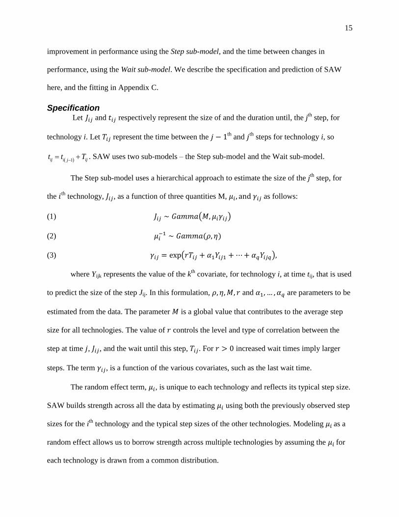
improvement in performance using the Step sub-model, and the time between changes in
performance, using the Wait sub-model. We describe the specification and prediction of SAW
here, and the fitting in Appendix C.
Specification Let and respectively represent the size of and the duration until, the j
th step, for
technology i. Let represent the time between the th and th
steps for technology i, so
1ij iji jt t T
. SAW uses two sub-models – the Step sub-model and the Wait sub-model.
The Step sub-model uses a hierarchical approach to estimate the size of the jth
step, for
the th technology, , as a function of three quantities M, as follows:
(1) ( )
(2)
(3) ( )
where Yijk represents the value of the kth
covariate, for technology i, at time tij, that is used
to predict the size of the step Jij. In this formulation, and are parameters to be
estimated from the data. The parameter is a global value that contributes to the average step
size for all technologies. The value of controls the level and type of correlation between the
step at time , , and the wait until this step, . For increased wait times imply larger
steps. The term , is a function of the various covariates, such as the last wait time.
The random effect term, , is unique to each technology and reflects its typical step size.
SAW builds strength across all the data by estimating using both the previously observed step
sizes for the ith
technology and the typical step sizes of the other technologies. Modeling as a
random effect allows us to borrow strength across multiple technologies by assuming the for
each technology is drawn from a common distribution.

16
In theory, one could model Jij or as coming from a variety of distributions. However,
the Gamma distribution has the advantage that: a) it is extremely flexible (it can model the
memoryless exponential and the chi-square distributions, and provides good approximations to
Normal and t-distributions). b) Using a Gamma allows us to calculate an exact likelihood
function for the Step and Wait sub-models which, in turn, provide a relatively simple way of
fitting the models by computing the maximum likelihood estimates. For a given the expected
step size is a function of the covariates, , the wait time, , and .
( |
Hence, a technology with a small will tend to have small step sizes, and vice-versa, but
this effect can be moderated by the observed covariates (e.g. a large investment in research and
development at time ) through the parameter . Since , and provide
information about the typical step size over all technologies. However, the individual covariates
for each technology will also affect the step size. The coefficients, dictate the
relationship between the covariates and the step size so, for example, a positive value for
indicates that increases in the kth
covariate are associated with larger step sizes while
would suggest no relationship.
The Wait sub-model works in a similar fashion, estimating the wait until the j+1th
step
for technology i, Ti,(j+1), as a function of three quantities, and as follows:
( )
where Xijk represents the value of the kth
covariate used to predict Tij for technology i at
time tij and and are parameters. The parameter is a global value that
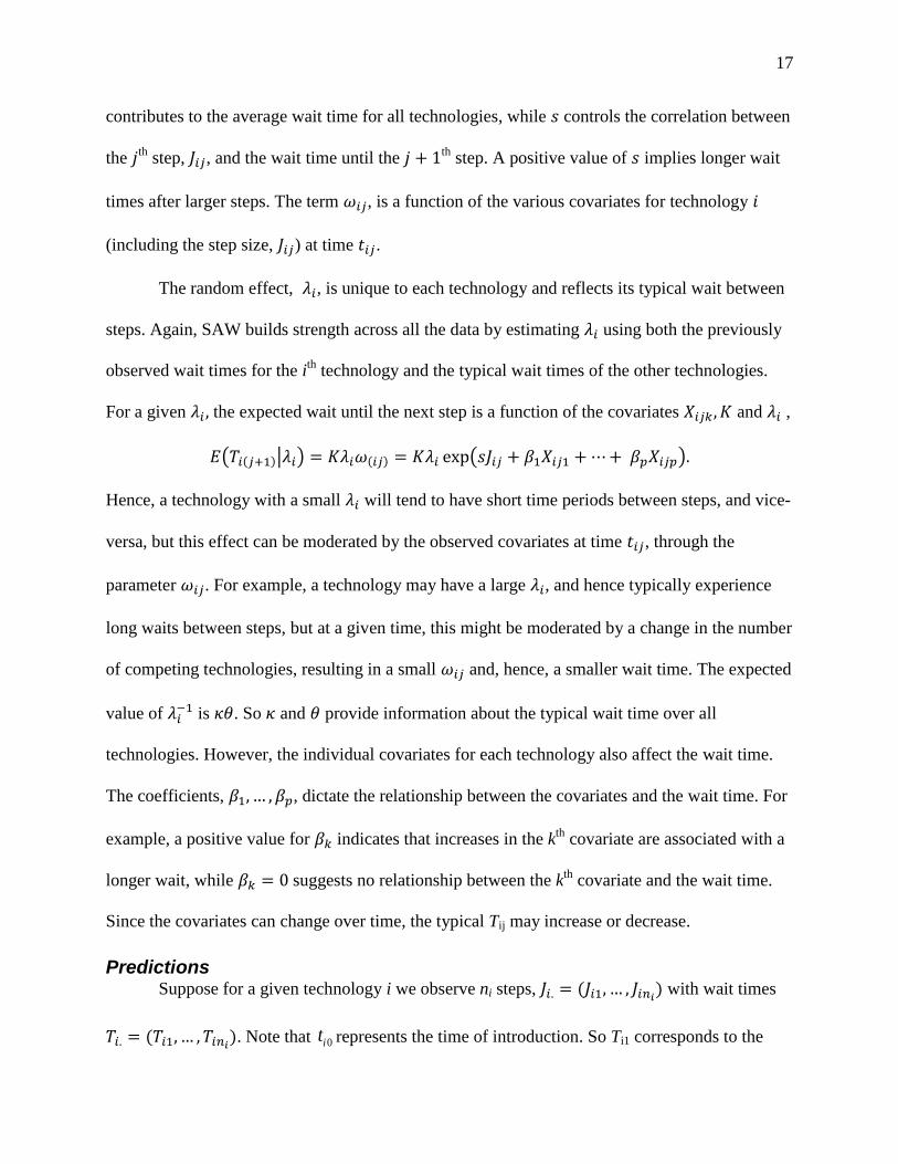
17
contributes to the average wait time for all technologies, while controls the correlation between
the th step, , and the wait time until the th
step. A positive value of implies longer wait
times after larger steps. The term , is a function of the various covariates for technology
(including the step size, ) at time .
The random effect, , is unique to each technology and reflects its typical wait between
steps. Again, SAW builds strength across all the data by estimating using both the previously
observed wait times for the ith
technology and the typical wait times of the other technologies.
For a given the expected wait until the next step is a function of the covariates and ,
( | ) ( )
Hence, a technology with a small will tend to have short time periods between steps, and vice-
versa, but this effect can be moderated by the observed covariates at time , through the
parameter . For example, a technology may have a large , and hence typically experience
long waits between steps, but at a given time, this might be moderated by a change in the number
of competing technologies, resulting in a small and, hence, a smaller wait time. The expected
value of
is . So and provide information about the typical wait time over all
technologies. However, the individual covariates for each technology also affect the wait time.
The coefficients, , dictate the relationship between the covariates and the wait time. For
example, a positive value for indicates that increases in the kth
covariate are associated with a
longer wait, while suggests no relationship between the kth
covariate and the wait time.
Since the covariates can change over time, the typical Tij may increase or decrease.
Predictions Suppose for a given technology i we observe ni steps,
with wait times
. Note that 0it represents the time of introduction. So Ti1 corresponds to the

18
duration from introduction of the technology until the first step, and Ji1 is the size of the first step.
Then natural estimates for the size of the next step, , and the wait until the next step,
, are ( | ) and ( | ). Using the Step sub-model given by Equations (1)
through (3), by the law of iterated expectations and the fact that has a gamma distribution,
( | ) ( ( | )| ) ( )
In order to compute the final expectation we need to derive the expected value of . The
distribution of conditional on is given by
∏ ( )
( ∑
)
(
)
( (
∑
))
Hence (
∑
) but the expected value of the inverse
of a Gamma ( random variable is equal to
. Therefore
∑
and the
expected size of the next step conditional on previous steps is
( | )
∑
.
Similarly, using the Wait sub-model given by Equations (4) through (6) the expected wait
until the next step conditional on previous steps is (derivation is identical to that for (7)),
(8) ( | )
∑
.
19
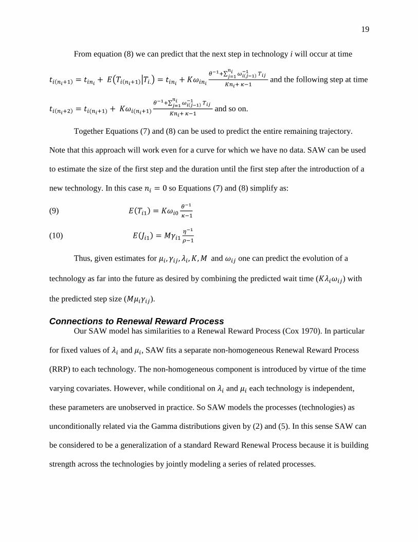
From equation (8) we can predict that the next step in technology i will occur at time
( | )
∑
and the following step at time
∑
and so on.
Together Equations (7) and (8) can be used to predict the entire remaining trajectory.
Note that this approach will work even for a curve for which we have no data. SAW can be used
to estimate the size of the first step and the duration until the first step after the introduction of a
new technology. In this case so Equations (7) and (8) simplify as:
(9)
(10)
Thus, given estimates for and one can predict the evolution of a
technology as far into the future as desired by combining the predicted wait time ( ) with
the predicted step size ( ).
Connections to Renewal Reward Process Our SAW model has similarities to a Renewal Reward Process (Cox 1970). In particular
for fixed values of and , SAW fits a separate non-homogeneous Renewal Reward Process
(RRP) to each technology. The non-homogeneous component is introduced by virtue of the time
varying covariates. However, while conditional on and each technology is independent,
these parameters are unobserved in practice. So SAW models the processes (technologies) as
unconditionally related via the Gamma distributions given by (2) and (5). In this sense SAW can
be considered to be a generalization of a standard Reward Renewal Process because it is building
strength across the technologies by jointly modeling a series of related processes.

20
Extensions of the Exponential, Logistic, Bass and Gompertz' Models In their standard forms, the Exponential, Logistic, Bass, and Gompertz models are all fit
individually to a single technology, and do not incorporate covariates in their specification. This
specification places them at a potential disadvantage relative to SAW, which both utilizes the
covariate information and builds strength across technologies by fitting all curves
simultaneously. In order to ensure a fair comparison we fit modified versions of these methods.
In particular we implemented two new versions of each approach.
In the first implementation, we used a non-linear mixed effects model (Pinheiro and
Bates, 2000), which fitted the standard functional forms of each method but modeled the various
parameters as random effects coming from a Gaussian distribution. The parameters for the
Gaussian distribution were estimated using all technologies simultaneously. Hence it built
strength across technologies in a similar fashion to SAW. Our second implementation also
modeled the parameters using a random effects formulation; but, in addition, incorporated the
covariates as a multiplicative adjustment to the original prediction. In this implementation we
modeled each technology using,
(11) ( ) ( ∑ )
where is the performance of technology at time , is the general formulation of the
Exponential, Logistic, Bass, or Gompertz model, exclusive of covariates, and is the th
covariate for technology at time . For example, the Exponential model, (11) becomes,
( ∑
)
with and modeled as coming from a Gaussian distribution. Equivalently, using a log
transformation,

21
∑
When is set to the Bass Model (11) has a similar form to the Generalized Bass Model
(Bass et al. 1994) though the latter method does not use a mixed effects fitting procedure.
We used a multiplicative covariate adjustment to because this ensured the basic shape
for each model was maintained while still allowing the covariates to influence the fit. This
second implementation had the twin advantages of building strength by simultaneously fitting all
curves and incorporating the covariates. Hence, these models can be seen as a direct competitor
to SAW. To our knowledge, neither the first nor second mixed effects formulations have been
previously implemented in such a setting, though in the Bass . So our specification can be
considered as a contribution in its own right. For more details of our fitting procedure see
Appendix B.
Method This section describes the data collection and the method of prediction.
Data We collected data on 26 technologies drawn from six markets - external lighting, desktop
printers, display monitors, desktop memory, data transfer, and automotive battery technologies
(see Table 2). We chose these six markets to ensure sufficiently long periods of study, wide
variety of technologies, and diversity of markets. We collected the data using the historical
method (Sood and Tellis 2005). The primary sources of our data are technical journals, white
papers, press releases, timelines of major firms, records in museums on the development of
industries, and annual reports of industry associations.
For each technology, we collected the performance of the technology on the most
important attribute to consumers – the primary basis of competition among technologies within a
22
market (see Table 2). We identified these important attributes based on articles collected through
the historical method. We recorded the maximum performance for any commercialized product
based on the technology at each time period. Our sample includes technologies introduced more
than a hundred years ago and those introduced only in the last decade. It also includes markets
from basic utilities, medical therapeutics, and the digital industry. Figure 1 shows the
performance of all technologies in three of the six markets.
We define a step as an improvement in performance however small, of any product in the
market based on a technology. We make the following assumptions: 1) The performance of a
technology in the market is based on the best performance of any commercialized product based
on that technology. Because of constraints in production, competitive agreements, or regulation,
the performance of products in the market often does not change at all in some years. Hence the
performance curve is flat in these years. 2) We have identified all products in the market based
on all technologies. 3) The performance of these products is correctly reported by manufacturers.
We used the following rules to ensure reliable and consistent data. First, we measure the
performance of a technology based only on commercialized products of that technology. Second,
if two sources provide conflicting performance for a technology in a period, we choose the one
whose values are more consistent with the rest of the series. Third, if no record is available for a
certain year, but a later record confirms that performance has not changed since the last available
record, we assume that the performance has not changed in the intervening years. Fourth, if no
record is available for a certain year, but a later record confirms that performance has changed
since the last available record, we treat the intervening years as missing data. Using these rules,
we were able to collect data on only 804 technology years as compared to the total of 901
technology years in our original sample (89%).

23
Method of Prediction A direct comparison of the statistical models across markets on all these technologies is
not possible unless the performance plots are modified to convert absolute performance to some
sort of relative performance. Since we are interested in analyzing how a technology improves
over time, we calculate the ratio of current performance to its performance in the year of first
introduction. We fit all methods after transforming the data onto a log scale. This transformation
reduces skewness in the data and generally gave lower prediction errors for all methods. We
explain the specific procedure for carrying out the prediction in two parts: partitioning of sample
and evaluation of predictive accuracy.
Partitioning of Sample To test the accuracy of predictions for future technology innovation using SAW and the
six alternate models, we divided the technologies into training (in sample) and testing (out of
sample) time periods. We could use data on only 25 technologies because the ESL technology
had only one observation by 2009. For each technology, we aimed to predict the performance for
the most recent 5 years. The training period consisted of the remaining data (see Figure A2a in
Appendix A). For the SAW approach we fitted the model using the training observations for all
technologies except the one for which we wished to make predictions. We then used the training
observations from the curve for which we were forming predictions to make predictions using
equations (7) and (8). This approach guaranteed a fair comparison with the other models by
ensuring that the out of sample data for a particular curve was never used, directly or indirectly,
to form estimates for a given technology.
Evaluation of Predictive Accuracy We compare the predictions on the test time period with the actual evolution of the
technology using two measures. The first is the average absolute deviation (AAD),
24
∑ ̂
where is the length of the testing period, Pit is the performance level at time t of the testing
period, for technology i, and ̂ is the corresponding estimate using a given model.
The second approach standardizes the curves according to the absolute values of the
technology (Percentage AAD). This method scales the error relative to the level of performance
in the technology. Specifically we compute,
∑
| ̂|
We report the median values of AAD and Percentage AAD averaged over all the
technologies.
Results We first present the results on the drivers of technological change. Next, we compare the
performance of SAW with alternative models in predicting technology evolution. We then
present the findings on the step size, wait time, and growth rate for all technologies. Finally, we
present plots of the patterns of technology evolution for all markets combined.
Drivers of Technological Change Table 3 presents the parameter estimates for the Step and Wait sub-models. The year of
introduction covariate has a positive sign for the Step sub-model but a negative sign for the Wait
sub-model. The results support H1 that products introduced in later years tend to have shorter
waits and larger steps.
The order of entry covariate has negative signs for both the Step and Wait sub-models.
The results indicate that, after controlling for year of entry, later entrants to a market tend to have

25
a shorter wait, but smaller steps. The negative coefficient for the step size is highly statistically
significant and is consistent with the preferential attraction theory (H2b).
The number of competing technologies covariate has a negative sign for the Step sub-
model and a positive sign for the Wait sub-model. The results suggest that after controlling for
the effects above, our results support H3a and reject H3b.
The number of prior steps covariate has a negative sign for both the Step and Wait sub-
models. The results support H4 and suggest that technologies that have a number of prior steps
continue to have small steps that happen at frequent intervals.
The average prior wait time covariate has a positive sign for the Step sub-model but a
slightly negative sign for the Wait sub-model. The results partially support H5; suggesting that,
after conditioning on the other covariates, technologies with long average prior wait time also
have larger step sizes but may not continue to have long wait times.
Finally, the last step size and the last wait time covariates are statistically significant in
the Step sub-model; providing evidence that there is a correlation between step sizes and wait
times, even after adjusting for the other covariates.
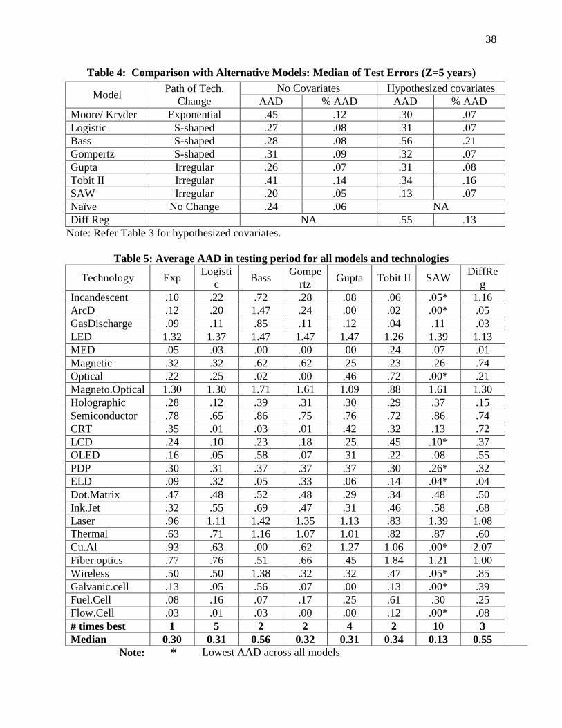
Comparison with Alternative Models Table 4 presents the median errors, over all technologies, comparing SAW with the
alternative models. We use the final five years for each technology as the testing period, i.e. Z=5.
We found that the alternative models all generally gave superior results using the log
transformed data so we report only these results. We also adjusted the competing methods so that
their predicted curve passed through the final training data point (see Figures A2b and A2c in
Appendix A). This generally gave superior results and made the models comparable to SAW,
which forms its predictions in the holdout period starting from the final training data point.
26
Table 4 contains two sets of results for each method. The first is the random effects fit
with no covariates while the second is the fit that incorporates the covariates from Table 3 using
(11). Among the models without covariates, SAW is significantly superior on both metrics.
When incorporating covariates, SAW improves further on the AAD metric, both in absolute
terms and relative to the competing methods. SAW is the best in AAD and equal to the best in
percentage AAD. Figure 2 plots the median AAD by year for models with covariates and
demonstrates that SAW outperforms most models in every year during the testing period. The
only exceptions are in 2005 and 2006, where the SAW and Gupta models both have zero AAD.
In all other years, and for all other methods, SAW is superior. We also compare the per
technology performance of SAW relative to the competing methods (see table 5). The SAW
model is first equal in performance on 40% of technologies, and has the lowest Median AAD
across all technologies for the 5 hold-out (most recent) years.
We also implemented the Exponential, Logistic, Bass, and Gompertz models using fixed
effects for the parameters, i.e. fitting the models separately to each curve. The results (not shown
here) were generally inferior to those reported in Table 4, suggesting that building strength by
fitting all curves simultaneously using random effects improves prediction accuracy. However,
since the alternate models were still inferior to SAW, we can conclude that SAW is performing
well partly because of its ability to build strength across technologies but also because of its
functional form which more accurately matches the observed data.
Step Size, Wait Time, and Growth Rate Equations (7) and (8) provide predicted step size and wait times which can be used to
predict the future evolution of a technology. Table 6 presents the average predicted step size, on
a log scale, and wait time, in years, for each technology (Columns 4 and 5). By taking the ratio
of predicted step size and wait time, we can also assess the average long run growth rate for each
27
technology (Column 6). The final column of Table 6 contains the estimates for , the exponent
when using a fixed effects model to fit an exponential curve to each technology, along with the
associated standard error, . Kryder’s law predicts that
while Moore’s
law implies
. Almost all technologies exhibited rates of growth considerably
slower than these values. The lone exceptions were the Fiber optics and Wireless technologies
which had estimated coefficients of and respectively. Thus, contrary to
claims in the literature, Kryder’s Law and Moore’s Law appear to be neither applicable to the
magnetic storage technology nor generalizable across markets.
Figure 3 provides a plot of the predicted step sizes and wait times for each of the 25
technologies on a two-dimensional graph. Several aspects stand out: First, there is clear
clustering, with technologies from the same markets generally showing similar predicted step
sizes and wait times. We might expect this form of clustering since technologies within the same
market will tend to have similar properties. Second, the unconditional correlation between step
size and wait time is negative (-0.32).
Figures A3a and A3b, in the Appendix A, plot the step size and wait times for each
technology as a function of calendar year respectively. The positive slope of the trend line in
Figure A3a suggests that the step size is increasing over time and the negative slope in Figure
A3b suggests that the wait time is decreasing over time. Figure A3c plots the growth rate (on a
log scale) over calendar time and shows a very clear trend of exponentially increasing growth
rates over calendar time, with a correlation of over 0.6 with a p-value below 1%. These results
suggest that technology evolution is occurring at a faster pace with calendar time.
Discussion This section summarizes the findings and discusses the implications and limitations.
28
Summary of Findings The current research leads to four major findings:
1. The traditional laws of technology evolution like Moore's Law and Kryder's law do not
generalize across markets; none holds for all technologies even in a single market.
2. SAW produces superior predictions over traditional methods, such as the Bass model or
Gompertz law, and can form predictions for a completely new technology, by incorporating
information from other categories on time varying covariates.
3. The signs of the significant drivers of technology evolution suggest that:
i. recent technologies improve at a faster rate than old technologies;
ii. as the number of competitors increases, performance of technologies increases in
smaller steps and longer waits;
iii. later entrants to a market and technologies that have a number of prior steps tend to
have smaller steps and shorter waits
iv. technologies with long average prior wait time continue to have large step sizes
4. Technologies cluster in their performance by market.
Implications This study has several implications for managers. First, our results suggest that popular
laws and models like Moore’s Law, Kryder’s Law, Gompertz Law, and the logistic model are
naive generalizations of what seems to be a complex phenomenon. Such theories make simplistic
assumptions about the path of technology evolution (e.g., exponential or S-shaped), and so are
inadequate in predicting technology change well. Surprisingly, over the period covered in our
analysis, it took 28 months for magnetic storage technology to double in performance, which is
much longer than the commonly espoused versions of Moore’s law claiming doubling every 18
months (recent) or 12 months (original). Hence, while such laws may serve as long term

29
guideposts for industry evolution, using them to predict the performance of a technology is quite
risky and potentially misleading. On the other hand, SAW explicitly models the discontinuous
nature of the technology evolution curves observed empirically.
Second, SAW can help managers to reduce the nature and extent of uncertainty regarding
the future path of technology evolution. SAW can be easily fit by a simple maximum likelihood
approach and incorporates time-varying covariates for each technology. Thus, managers can use
it to assess the nature of the threat posed by a competing technology by classifying it as one that
is a long-wait-small-step technology or vice versa. As an example, consider the competition
between LCD and CRT monitors (see Figure 1b). Sony kept investing in CRT even after LCD
first crossed CRT in performance in 1996. Instead of considering LCD, Sony introduced the FD
Trinitron/WEGA series, a flat version of the CRT. CRT crossed LCD for a few years, but
ultimately lost decisively to LCD in 2001. In contrast, by backing LCD, Samsung grew to be the
world's largest manufacturer of LCD, while the former leader Sony had to seek a joint venture
with Samsung in 2006 to manufacture LCD. Prediction of the next step size and wait time using
SAW could have helped Sony’s managers make a timely investment in LCD technology.
Third, SAW overcomes limitations of prior models of depending on only environmental
scanning (e.g., survey or the Delphi method) or extrapolation (e.g., trend analysis). SAW
incorporates both environmental scanning by incorporating data from multiple technologies and
extrapolation by incorporating past data from the target technology in making predictions.
Further, SAW is flexible enough to allow for large periods of no change punctuated by big steps
or small periods of small changes approximating a smooth curve. As such, it partially resolves
the controversy in the literature between technology evolution via a smooth curve (Basalla 1988;
Dosi, 1982) or via stable periods punctuated with big steps (Eldredge and Gould 1972; Tushman
30
and Anderson 1986). For example, inkjet printers became the dominant technology in the market
even though they had the lowest performance at introduction through a series of small but
frequent steps.
Fourth, our results suggest that the competitive landscape is becoming more intense. An
increasing number of new technologies are entering the market. The rate of technology evolution
is increasing at a faster pace. Thus, managers need a method and model to predict technology
evolution to guide their multi-million dollar investments. SAW serves such a purpose. SAW can
easily make predictions for a new technology with no prior data. This discussion brings us back
to the key question that managers face. Which technology to back? In GM’s case, it turned out to
be a billion dollar question. GM spent over a billion dollars on the hydrogen fuel cell. Yet the
technology that leapt ahead in the 2000s was Lithium-ion. Tesla based its battery on the Lithium-
ion and had a car on the market in 2006. GM saw the need for Lithium-ion only after the Tesla
was launched and launched a car using a Lithium-ion battery only in December 2010. Many
firms were taken by surprise by the sudden dominance of Lithium-ion. Managers could possibly
have presaged the improvements in Lithium-ion technology before 2006 by using our model.
Limitations This study has four limitations. First we had to limit our analysis to only six markets due
to the time and difficulty of data collection. Second, our analysis does not include the impact of
investments in R&D on technology evolution. This is a limitation of the data, rather than of
SAW, since it could certainly include R&D budgets as a covariate, which should increase its
predictive accuracy even more. Third, our analysis does not include the cost of the technology to
buyers. Fourth, it is not possible to exactly estimate the step size and wait times for the years
with missing data. However, given the small percentage of such data this is unlikely to have a
significant effect on the results. Fifth, we assume firms announce all improvements in
31
performance and there are no minor improvements between steps. A possible extension may
relax this assumption and allow for a low level of growth during the wait period. All of these
limitations are potential opportunities for future research.

32
REFERENCES
Abernathy W. J. and Utterback J. M. (1978), "Patterns of Industrial Innovation" Technology
Review 80; 7.
Adner R. (2002), “When are Technologies Disruptive: A Demand-based View of the Emergence
of Competition,” Strategic Management Journal, 23: 667-88.
Armstrong J. S. (2005), “Forecasting by Extrapolation: Conclusions from 25 Years of Research,”
General Economics and Teaching, EconWPA.
Arrow K.J. (1962), “Economic Welfare and the Allocation of Resources to Invention,” in R.R.
Nelson (ed.), The Rate and Direction of Economic Activity, Princeton Univ Press, N.Y.
Balachandra R. (1980), “Technological forecasting: who does it and how useful is it?
Technological Forecasting and Social Change 16 (1980), 75–85.
Basalla G. (1988), “The Evolution of Technology,” Cambridge Univ. Press, Cambridge, U.K.
Bass F.M. (1969), “A New Product Growth for Model Consumer Durables,” Management
Science 15, 215–227.
Bass F.M., Krishnan, T.V. and Jain, D.C. (1994), “Why the Bass Model Fits without Decision
Variables,” Marketing Science, (13) (3), 203-223.
Brown R. (1992), “Managing ‘S’ Curves of Innovation,” Journal of Consumer Marketing, 9 (1),
61–73.
Chandy R. K. and Tellis G. J. (2000), “The Incumbent's Curse? Incumbency, Size, and Radical
Product Innovation," Journal of Marketing, 64 (3), 1-17.
Cox, D. (1970), “Renewal Theory,” London: Methuen & Co.
D'Aveni R.A. (1994), “Hypercompetition: Managing the Dynamics of Strategic Maneuvering,”
New York: The Free Press.
Dosi G. (1982), “Technological Paradigms and Technological Trajectories: The Determinants
and Directions of Technical Change and the Transformation of the Economy” in C.
Freeman (ed.) Long Waves in the World Economy, London.
33
Edwards C. (2008) “The Many Lives Of Moore's Law [Moore's Law - Electronics]” Engineering
& Technology, 3, 1, 36-9.
Eldredge N. and Gould S. J. (1972), “Punctuated Equilibria: An Alternative to Phyletic
Gradualism,” in: Dobzhansky, T. et al.: Models in Paleobiology, Freeman, Cooper and
Co., 82-115.
Fellner W. (1961), “Two Propositions in the Theory of Induced Innovations,” Economic Journal,
71 (282), 305-308.
Fleming L. (2001), “Recombinant Uncertainty in Technological Search,” Management Science,
47(1): 117-132.
Foster R.D. (1986), “Innovation: The Attacker's Advantage,” New York: Summit Books.
Gersick C. J. G. (1991), “Revolutionary Change Theories: A Multilevel Exploration of the
Punctuated Equilibrium Paradigm,” The Academy of Management Review, 16, 1, 10-36
Golder Peter N. and Gerard J. Tellis (1993), “Pioneering Advantage: Marketing Logic or
Marketing Legend,” Journal of Marketing Research.
Golder, Peter N and Gerard J. Tellis (2004), “Going, Going, Gone: Cascades, Diffusion, and
Turning Points of the Product Life Cycle,” Marketing Science, 23, 2 (180-191).
Gompertz B. (1825), “On the Nature of the Function Expressive of the Law of Human Mortality,
and on a New Mode of Determining the Value of Life Contingencies,” Philosophical
Transactions of the Royal Society of London 115: 513–585
Grochowski E (1998), “Emerging Trends in Data Storage on Magnetic Hard Disk Drives,”
Datatech, 11.
Gupta, Sunil (1988), “Impact of Sales Promotions on When, What, and How Much to Buy,”
Journal of Marketing Research 25: 342-355
Hauser John, Gerard J. Tellis and Abbie Griffin (2007), “Research on Innovation and New
Products: A Review and Agenda for Marketing Science,” Marketing Science, 25, 6, 687-
717.
34
Henderson, R.M, and Clark K.B. (1990), “Architectural Innovation: The Reconfiguration of
Existing Product Technologies and the Failure of Established Firms." Administrative
Science Quarterly, 35, 9-30.
Lambkin M. (1988), “Order of Entry and Performance in New Markets,” Strategic Management
Journal, Vol. 9, Special Issue: Strategy Content Research. (Summer), pp. 127-140.
Levinthal, D. (1998) “The Slow Pace of Rapid Technological Change: Gradualism and
Punctuation in Technological Change,” Industrial and Corporate Change, 7: 217-247.
Makridakis S., Anderson A., Carbone R., Fildes R., Hibon M., Lewandowski R., Newton J.,
Parzen P., and Winkler R. (1982), “The Accuracy of Extrapolation (Time Series)
Methods: Results of a Forecasting Competition,” Journal of Forecasting, NY 1, 111–53.
Martino J.P. (2003), “A Review Of Selected Advances In Technological Forecasting,”
Technological Forecasting and Social Change 70 (8), 719–33.
Meade N. and Islam T. (1995), “Forecasting With Growth Curves: An Empirical Comparison,”
International Journal of Forecasting, 11, 199–215.
____ and ____ (1998), “Technological Forecasting – Model Selection, Model Stability, And
Combining Models,” Management Science, 44, 1115–30.
____ and ____ (2006), “Modeling And Forecasting The Diffusion Of Innovation – A 25 Year
Review,” International Journal of Forecasting, 22 (3), 519–45.
Mollick E. (2006), “Establishing Moore's Law” IEEE Annals of the History of Computing, 62-75
Moore G. E. (1965), "Cramming More Components Onto Integrated Circuits," Electronics, Vol.
38, No. 8 (19 April), at http://www.intel.com/research/silicon/moorespaper.pdf.
____ (1975) “Progress In Digital Integrated Electronics,” IEEE, IEDM Tech Digest, 11-3.
____ (1997), "An Update on Moore's Law," Intel Developer Forum Keynote (30 September).
____ (2003), “No Exponential Is Forever: But "Forever" Can Be Delayed!” Solid-State Circuits
Conference, 2003, Digest of Technical Papers, IEEE International, 1, 20-23.
Nelson, RR and Winter SG, (1977), “'In search of useful theory of innovation,” Research Policy,
6, 36-76
35
Pinheiro José C. and Douglas M. Bates (2000), “Mixed-Effects Models in S and S-PLUS,”
Statistics and Computing Series, Springer-Verlag, New York, NY.
Rogers E. M. (1962), “Diffusion of Innovations,” New York: Free Press.
Rosenberg, N. (1969), “The Direction of Technological Change: Inducement Mechanisms and
Focusing Devices,” Economic Development and Cultural Change, 18, 1-24.
Sahal D. (1981), "Alternative Conceptions of Technology,” Research Policy, 10 (1), 2-24
Schaller R.R. (1997), “Moore's Law: Past, Present and Future” Spectrum, IEEE, 34, 6, June, 52-9
Scherer, F.M. (1967), “Market Structure and the Employment of Scientists and Engineers,”
American Economic Review, 57 (June), pp. 524-531.
Scherer, F.M. and Ross D. (1990), “Industrial Market Structure and Economic Performance,”
HM
Shacklett M. (2008), “Storage Density & Kryder's Law”, Byte and Switch News Analysis, 11, 19
Sood A. and Tellis G. J. (2005), “Technological Evolution and Radical Innovations,” Journal of
Marketing, 69, 3, 152-68.
___ and ___ (2011), “Demystifying Disruption: A New Model for Understanding and Predicting
Disruptive Technologies,” Marketing Science, 2011 30: 339-354
___, Gareth James, and ____ (2009) "Functional Regression: A New Model for Predicting
Market Penetration of New Products", Marketing Science, 2009 28: 36-51.
Tashman L. J. (2000), “Out-of-Sample Tests of Forecasting Accuracy: An Analysis and
Review,” International Journal of Forecasting, 16, 4, 437-50
Tellis, G. (2008). Important research questions in technology and innovation. Industrial
Marketing Management, 37, 629 – 632
Tushman M. L. and Anderson P. (1986), “Technological Discontinuities and Organizational
Environments,” Administrative Science Quarterly, 31, 439-65.
____ and Romanelli E. (1985), “Organizational Evolution: A Metamorphosis Model of
Convergence and Reorientation," Research in Organizational Behavior, 171 - 222.
36
Urban G.L., Theresa C., Steven G. and Zofia M. (1986), “Market Share Rewards to Pioneering
Brands: An Empirical Analysis and Strategic Implications,” Management Science, Vol.
32, 6, 645-659.
Utterback J. and William Abernathy. (1975), “A Dynamic Model of Process and Product
Innovation," Omega, 33: 639-656.
Walter C. (2005) “Kryder's Law” Scientific American July 25,
Wolff M.F. (2004), “Chase Moore’s Law Inventors Urged,” Research Technology Management,
47, 1, 6.
Wollin A. (1999), “Punctuated equilibrium: Reconciling Theory of Revolutionary and
Incremental Change,” Systems Research and Behavioral Science, 16: 359-67.
Young P. and Ord K. (1989), “Model Selection and Estimation of Technological Growth
Curves,” International Journal of Forecasting, 5, 501-13.
____ (1993), “Technological Growth Curves: A Competition of Forecasting Models,”
Technological Forecasting and Social Change, 44, 375 –89.
37
Table 1: Unifying Framework for Models for Predicting Technology Evolution
Smooth
(Continuous)
Discontinuous
(Irregular)
Symmetric Logistic, Bass, Gompertz
(S-shaped) NA
Asymmetric Moore, Kryder
(Exponential-shaped)
SAW, Tobit, Gupta, Diff Reg
(irregular step sizes with
irregular wait times)
Table 2: Technologies Sampled and Primary Dimensions of Competition*
Market Primary Basis of Competition Metric
External Lighting Lighting Efficacy Lumens per Watt
Desktop Memory Storage capacity Bytes per square inch
Display Monitors Screen resolution Dots per square inch
Desktop Printers Print resolution Pixels per square inch
Data Transfer Transfer Speed Megabits per second
Automotive Battery Energy Density Watt-hour/kg
Note: * Adapted from Sood and Tellis (2005)
Table 3: Drivers of Step Size and Wait Time
Covariate Step Size Wait Time
Est. t-val Est. t-val
Year of Introduction (H1) .19 39.7 -.12 -247.3
Order of Entry (H2) -.31 -8.0 -.05 -1.3
Number of Competing Technologies (H3) -.11 -3.0 .42 12.4
No of Prior Steps (H4) -.01 -1.3 -.06 -6.4
Average Prior Wait Time (H5) .08 3.4 -.003 -.1
Last Step Size (r – Equation 3) .02 2.9 .002 .3
Last Wait Time (s – Equation 6) -.04 -2.8 -.01 -.8
38
Table 4: Comparison with Alternative Models: Median of Test Errors (Z=5 years)
Model Path of Tech.
Change
No Covariates Hypothesized covariates
AAD % AAD AAD % AAD
Moore/ Kryder Exponential .45 .12 .30 .07
Logistic S-shaped .27 .08 .31 .07
Bass S-shaped .28 .08 .56 .21
Gompertz S-shaped .31 .09 .32 .07
Gupta Irregular .26 .07 .31 .08
Tobit II Irregular .41 .14 .34 .16
SAW Irregular .20 .05 .13 .07
Naïve No Change .24 .06 NA
Diff Reg NA .55 .13
Note: Refer Table 3 for hypothesized covariates.
Table 5: Average AAD in testing period for all models and technologies
Technology Exp Logisti
c Bass
Gompe
rtz Gupta Tobit II SAW
DiffRe
g
Incandescent .10 .22 .72 .28 .08 .06 .05* 1.16
ArcD .12 .20 1.47 .24 .00 .02 .00* .05
GasDischarge .09 .11 .85 .11 .12 .04 .11 .03
LED 1.32 1.37 1.47 1.47 1.47 1.26 1.39 1.13
MED .05 .03 .00 .00 .00 .24 .07 .01
Magnetic .32 .32 .62 .62 .25 .23 .26 .74
Optical .22 .25 .02 .00 .46 .72 .00* .21
Magneto.Optical 1.30 1.30 1.71 1.61 1.09 .88 1.61 1.30
Holographic .28 .12 .39 .31 .30 .29 .37 .15
Semiconductor .78 .65 .86 .75 .76 .72 .86 .74
CRT .35 .01 .03 .01 .42 .32 .13 .72
LCD .24 .10 .23 .18 .25 .45 .10* .37
OLED .16 .05 .58 .07 .31 .22 .08 .55
PDP .30 .31 .37 .37 .37 .30 .26* .32
ELD .09 .32 .05 .33 .06 .14 .04* .04
Dot.Matrix .47 .48 .52 .48 .29 .34 .48 .50
Ink.Jet .32 .55 .69 .47 .31 .46 .58 .68
Laser .96 1.11 1.42 1.35 1.13 .83 1.39 1.08
Thermal .63 .71 1.16 1.07 1.01 .82 .87 .60
Cu.Al .93 .63 .00 .62 1.27 1.06 .00* 2.07
Fiber.optics .77 .76 .51 .66 .45 1.84 1.21 1.00
Wireless .50 .50 1.38 .32 .32 .47 .05* .85
Galvanic.cell .13 .05 .56 .07 .00 .13 .00* .39
Fuel.Cell .08 .16 .07 .17 .25 .61 .30 .25
Flow.Cell .03 .01 .03 .00 .00 .12 .00* .08
# times best 1 5 2 2 4 2 10 3
Median 0.30 0.31 0.56 0.32 0.31 0.34 0.13 0.55
Note: * Lowest AAD across all models

39
Table 6: Step Size, Wait Times, and Growth Rates
Category Technology Year of
Introduction
Mean
Step Size
Mean
Wait Time
Growth
Rate
From SAW
(Equations 7
and 8)
Growth Rate
from Exponential
Model (SE)
External
Lighting
Incandescent 1879 0.11 19.73 0.01 0.02 (0.001)
Arc Discharge 1908 0.10 10.11 0.01 0.03 (0.001)
Gas Discharge 1932 0.27 14.02 0.02 0.02 (0.001)
LED 1965 0.34 3.63 0.09 0.13 (0.005)
MED 1989 0.34 6.98 0.05 0.01 (0.002)
Desktop
memory
Magnetic 1937 0.35 1.25 0.28 0.31 (0.007)
Optical 1982 1.28 10.83 0.12 0.12 (0.011)
MO 1986 0.88 4.47 0.20 0.24 (0.011)
Holographic 2002 0.79 4.06 0.19 0.12 (0.017)
Semiconductor 2002 0.91 5.00 0.18 0.26 (0.066)
Display
Monitors
CRT 1929 0.38 3.59 0.10 0.19 (0.016)
LCD 1967 0.50 3.29 0.15 0.21 (0.011)
OLED 1971 0.52 5.13 0.10 0.11 (0.011)
PDP 1984 0.60 4.13 0.15 0.20 (0.018)
ELD 2004 0.47 4.52 0.10 0.02 (0.007)
Data
Transfer
Dot Matrix 1953 0.56 5.02 0.11 0.07 (0.005)
Ink Jet 1975 0.91 2.19 0.41 0.32 (0.013)
Laser 1976 0.83 5.21 0.16 0.19 (0.014)
Thermal 1979 0.69 3.37 0.20 0.29 (0.018)
Desktop
Printers
Cu Al 1962 2.47 5.17 0.48 0.38 (0.021)
Fiber Optics 1977 2.19 1.88 1.16 0.44 (0.016)
Wireless 1982 1.83 2.69 0.68 0.60 (0.051)
Automotive
Batteries
Galvanic Cell 1780 0.34 5.74 0.06 0.06 (0.008)
Fuel Cell 1838 0.49 2.62 0.19 0.10 (0.008)
Flow Cell 1980 0.30 7.60 0.04 0.02 (0.002)

40
Figure 1: Empirical Path of Technology Evolution In 3 Markets
Figure 1a: Desktop Memory
Figure 1b: Display Monitors
Figure 1c: Automotive Batteries
0.1
1.0
10.0
100.0
1000.0
10000.0
100000.0
1000000.0
19
69
19
71
19
73
1975
19
77
19
79
19
81
19
83
19
85
19
87
19
89
19
91
19
93
19
95
1997
19
99
20
01
20
03
20
05
20
07
20
09
Are
al D
en
sity
(M
bp
si) Magnetic Optical
Magneto-Optical Holographic
Semiconductor
0.0001
0.001
0.01
0.1
1
10
19
69
19
71
19
73
19
75
19
77
19
79
19
81
19
83
19
85
19
87
19
89
19
91
19
93
19
95
19
97
19
99
20
01
20
03
20
05
20
07
20
09
Scre
en R
eso
luti
on
('0
00
pix
els
psi
)
CRT LCD
OLED PDP
ELD
0
200
400
600
800
1000
1200
1400
1600
1800
2000
19…
19…
19…
19…
19…
19…
19…
19…
19…
19…
20…
20…
20…
20…
20…
Spec
ific
En
ergy
(kW
-Hr/
kg)
Flow Cell
Fuel Cell
Galvanic cell

41
Figure 2: Median AAD for Models with Covariates for 5 Year Prediction
Figure 3: Predicted Step Vs. Wait Patterns
0
0.1
0.2
0.3
0.4
0.5
0.6
0.7
0.8
0.9
1
2005 2006 2007 2008 2009
AA
D
Testing Period
Exponential Logistic
Bass Gompertz
Tobit II Gupta
SAW DiffReg
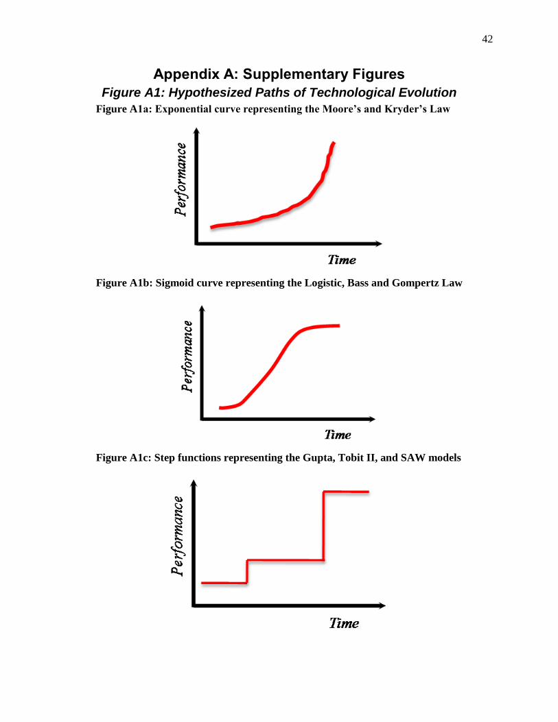
42
Appendix A: Supplementary Figures
Figure A1: Hypothesized Paths of Technological Evolution
Figure A1a: Exponential curve representing the Moore’s and Kryder’s Law
Figure A1b: Sigmoid curve representing the Logistic, Bass and Gompertz Law
Figure A1c: Step functions representing the Gupta, Tobit II, and SAW models

43
Figure A2: Experimental Setup
Figure A2a: Sampling of Technologies and Time Periods For Prediction
Figure A2b: Unconstrained Fits Figure A2c: Constrained Fits
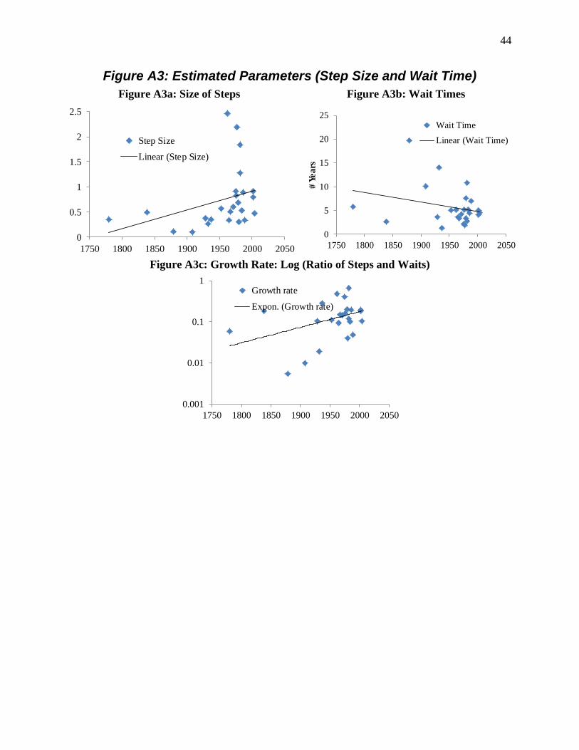
44
Figure A3: Estimated Parameters (Step Size and Wait Time)
Figure A3a: Size of Steps Figure A3b: Wait Times
Figure A3c: Growth Rate: Log (Ratio of Steps and Waits)
0
0.5
1
1.5
2
2.5
1750 1800 1850 1900 1950 2000 2050
Step Size
Linear (Step Size)
0
5
10
15
20
25
1750 1800 1850 1900 1950 2000 2050
# Y
ears
Wait Time
Linear (Wait Time)
0.001
0.01
0.1
1
1750 1800 1850 1900 1950 2000 2050
Growth rate
Expon. (Growth rate)
45
Appendix B:
Prediction and Fitting of Comparison Models In their standard forms, Moore’s law, Kryder’s law and the logistic, Bass, and Gompterz
model do not directly incorporate covariates into their predictions. In order to provide a
comparison with SAW, which does allow for the inclusion of covariates, we fit two modified
versions of these methods. In the first implementation we used a non-linear mixed effects model
which fit the standard functional forms of each method but modeled the various parameters as
random effects coming from a Gaussian distribution. The parameters for the Gaussian
distribution were estimated using all technologies simultaneously and hence built strength in a
similar fashion to SAW. Our second implementation of these methods also modeled the
parameters using a random effects formulation but in addition incorporated the covariates as a
multiplicative adjustment to the original prediction using (11). Next, we discuss both the Mixed
Effects Model and the Mixed Effects Model with Covariate Effects for each method. By
comparison the Gupta and Tobit II models involve covariates so must be fit to all curves
simultaneously to estimate the population level covariate coefficients.
Extensions of Moore’s Law and Kryder’s Law (Exponential Model)
Mixed Effects Model
Moore’s Law and Kryder’s Law each state that the rate of change in the performance of a
technology is exponential with given constants. Thus, if we model performance of the
technology as an exponential function of time, the coefficient of time represents the constant rate
at which the technology improves. To test the applicability of Moore’s Law and Kryder’s Law,
we model the relationship between time and technology performance using the following
exponential function:

46
where, is performance for technology at time , and and are modeled as
random variables coming from Gaussian distributions.
We estimate the coefficients for the exponential model associated with Moore’s Law and
Kryder’s Law using linear mixed effects software applied to the log-transformed data. Kryder’s
Law assumes
while Moore’s Law assumes
. After fitting the mixed
effects model to each technology we use the fitted parameters to form predictions and compare
the estimate for with that predicted by Kryder’s and Moore’s Laws.
Mixed Effects Model with Covariate Effects
Let represent different covariates measured at time . We
incorporate these covariates into the exponential model in a multiplicative fashion using the
following formulation,
(15) ( ∑
)
Note that the parameter are modeled as random effects because they are specific to a
particular technology but the coefficeints are treated as fixed effects because they are common
to all technologies.
Extensions of Logistic Model
Mixed Effects Model
The generalized form of the logistic curve is a relatively flexible model that can also
capture an S-shape of the path of technological evolution. This model has been widely used in
prior literature (e.g. Young 1993; Meade and Islam 1998).

47
where, is the performance of technology at time , and and are modeled as
random variables coming from Gaussian distributions.
We fit equation (16) using non-linear mixed effects software applied to the log-
transformed data.
Mixed Effects Model with Covariate Effects
We incorporate the covariates into the logistic model using a multiplicative formulation, thus
( ) ( ∑
)
Note that the parameters are modeled as random effects because they are
specific to a particular technology but the coefficients are treated as fixed effects because they
are common to all technologies.
Extensions of Bass Model
Mixed Effects Model
The Bass model (Bass 1969) is a special case of the Gamma/shifted-Gompertz
distribution that can capture an S-shape plus a variety of other shapes that approximate the S-
curve depending on the values of the parameters. We use the operational form of the Bass model
used previously for modeling technology evolution (Young and Ord 1989; Young 1993):
( )
where, is the performance of technology at time ,
is marginal performance improvement at time ,
and are modeled as random variables coming from a Gaussian distribution. We fit
equation (18) using non-linear mixed effects software applied to the log-transformed data.
Mixed Effects Model with Covariate Effects
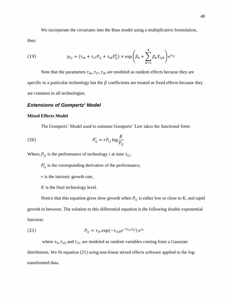
48
We incorporate the covariates into the Bass model using a multiplicative formulation,
thus:
( ∑
)
Note that the parameters are modeled as random effects because they are
specific to a particular technology but the coefficients are treated as fixed effects because they
are common to all technologies.
Extensions of Gompertz' Model
Mixed Effects Model
The Gompertz’ Model used to estimate Gompertz’ Law takes the functional form:
Where, is the performance of technology at time ,
is the corresponding derivative of the performance,
is the intrinsic growth rate,
is the final technology level.
Notice that this equation gives slow growth when is either low or close to K, and rapid
growth in between. The solution to this differential equation is the following double exponential
function:
where and are modeled as random variables coming from a Gaussian
distribution. We fit equation (21) using non-linear mixed effects software applied to the log-
transformed data.

49
Mixed Effects Model with Covariate Effects
We incorporate the covariates into the Gompertz model using a multiplicative
formulation, thus:
( ∑
)
Note that the parameters are modeled as random effects because they are
specific to a particular technology but the coefficients are treated as fixed effects because they
are common to all technologies.
Constrained Parameters
Several of the parameters in the above mentioned models are constrained to by positive. To
operationalize this constraint we parameterized the corresponding coefficients as
where was modeled as coming from a Gaussian distribution. This formulation ensured that
would always be positive.
Extensions of Gupta Model The interpurchase time model uses an Erlang-2 distribution to model the time until a
purchase, or in our case wait time until a jump in technology, with the Erlang parameter modeled
as a function of a set of explanatory variables. Specifically,
( )
where is the probability density, at time , of the wait until the next jump for technology
i, is the Erlang-2 scale parameter and is the th covariate at . The time until purchase,
or technology jump, is predicted using the Erlang-2 mean,
.
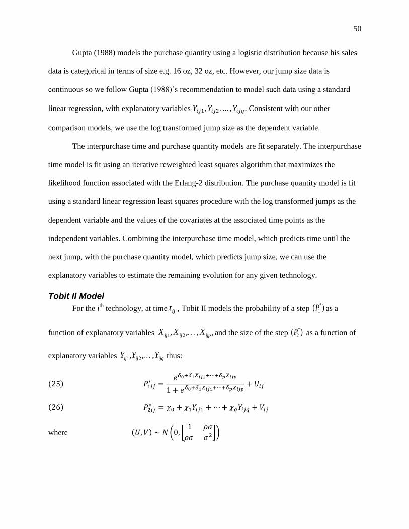
50
Gupta (1988) models the purchase quantity using a logistic distribution because his sales
data is categorical in terms of size e.g. 16 oz, 32 oz, etc. However, our jump size data is
continuous so we follow Gupta (1988)’s recommendation to model such data using a standard
linear regression, with explanatory variables . Consistent with our other
comparison models, we use the log transformed jump size as the dependent variable.
The interpurchase time and purchase quantity models are fit separately. The interpurchase
time model is fit using an iterative reweighted least squares algorithm that maximizes the
likelihood function associated with the Erlang-2 distribution. The purchase quantity model is fit
using a standard linear regression least squares procedure with the log transformed jumps as the
dependent variable and the values of the covariates at the associated time points as the
independent variables. Combining the interpurchase time model, which predicts time until the
next jump, with the purchase quantity model, which predicts jump size, we can use the
explanatory variables to estimate the remaining evolution for any given technology.
Tobit II Model
For the ith
technology, at time ijt , Tobit II models the probability of a step *
1( )P as a
function of explanatory variables 1 2, , , ,ij ij ijpX X X and the size of the step *
2( )P as a function of
explanatory variables 1 2, , ,ij ij ijqY Y Y thus:
where ( [
])
51
We observe a step conditional on the probability of a jump exceeding a cutoff value, for
example *
1 11( 0.1)ij ijP P always, but observe the size of step P2ij only when the step occurs i.e.,
1 1.ijP We use standard software to estimate the joint outcome – probability and size of step – in
the Tobit II model (Tellis 1988).

52
Appendix C: Fitting of SAW We provide details on fitting of SAW:
Fitting of SAW Fitting SAW requires estimating a number of parameters. We use a maximum likelihood
approach. Suppose we have observed ni steps of technology i at times 1, , .ii int t Let
represent the series of observed steps and
be the times between
these steps. In addition we assume covariates Xijk and Yijk have been observed at times tij.
Conditional on and the distribution of .iT is
(∏
) (
∑
)
Similarly, the distribution of conditional on and is
|
(
)
Hence, the distribution of .iT conditional on and is
(27)
(∏
) (
∑
)
(
)
(∏
)
( ∑
)
We can use Equation (27) to write down the log likelihood function,
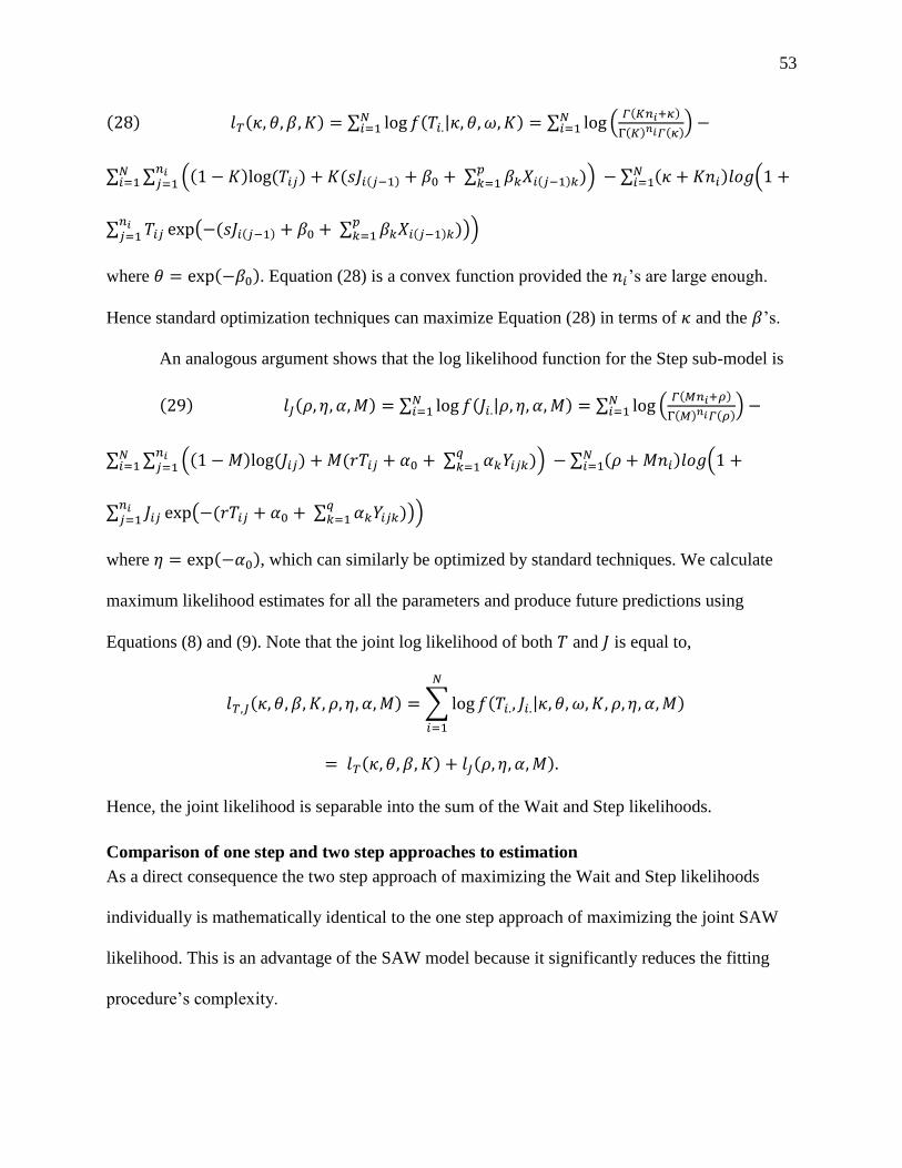
53
∑ ∑ (
)
∑ ∑ ( ∑ )
∑ (
∑ ( ∑ )
)
where . Equation (28) is a convex function provided the ’s are large enough.
Hence standard optimization techniques can maximize Equation (28) in terms of and the ’s.
An analogous argument shows that the log likelihood function for the Step sub-model is
∑ ∑ (
)
∑ ∑ ( ∑ )
∑ (
∑ ( ∑ )
)
where , which can similarly be optimized by standard techniques. We calculate
maximum likelihood estimates for all the parameters and produce future predictions using
Equations (8) and (9). Note that the joint log likelihood of both and is equal to,
∑
Hence, the joint likelihood is separable into the sum of the Wait and Step likelihoods.
Comparison of one step and two step approaches to estimation
As a direct consequence the two step approach of maximizing the Wait and Step likelihoods
individually is mathematically identical to the one step approach of maximizing the joint SAW
likelihood. This is an advantage of the SAW model because it significantly reduces the fitting
procedure’s complexity.
Related Documents