Predicting Student Loan Default for the University of ... · PDF filestudent loan default is a serious issue for borrowers, schools, lenders, and guarantors. Prior studies on the causes

27NASFAA JOURNAL OF STUDENT FINANCIAL AID

During spring 2001, Noel-Levitz created a student loan default

model for the University of Texas at Austin (UT Austin). The goal

of this project was to identify students most likely to default, to

identify as risk elements those characteristics that contributed to

student loan default, and to use these risk elements to plan and

implement targeted, pro-active interventions to prevent student

loan default. UT Austin supplied academic data for the project,

and the student loan guarantor Texas Guaranteed Student Loan

Corporation (TG) provided the data about borrowers from UT Aus-

tin who entered repayment between 1996 and 1999. Results

showed that student program completion, persistence, and suc-

cess were strong predictors of student loan default, as were race/

ethnicity, gender, and the school of enrollment at UT Austin These

results emphasize the role of student success and graduation in

eventual loan repayment. Interventions that focus on student per-

sistence and academic success were seen as the primary actions

needed to help prevent student loan default.

Over the past decade, total aid to students to financehigher education has increased by 117 % (College Board,2002). In 2002-2003, more than $105 billion in total

financial aid was provided from all sources (College Board, 2003).During the 1990s, the amount of grant aid doubled, while loanaid tripled. The share of grants decreased from 50% of total aidin 1991-1992 to 40% in 2001-2002, while the proportion of aidfrom loans increased from 47% to 54%. Graduate students usethree times as much loan aid as grant aid (College Board, 2002).In 2002-03, federal loans comprised 45% of total aid, amount-ing to $47.7 billion (College Board, 2002 & 2003). Overall, 29%of all undergraduates borrowed from some source to help fi-nance their postsecondary education in 1999-2000 (Clinedinst,Cunningham, & Merisotis, 2003).

Of the borrowers with Stafford Loans and/or Supple-mental Loans for Students (SLS), undergraduates at two-yearpublic colleges were the least likely to borrow (6%), followed bystudent borrowers at public four-year schools (35%), privatenot-for-profit four-year schools (43%), and private for-profit (pro-prietary) schools at 50% (Berkner, 2000).

Researchers have carefully examined the increasing loanexposure of students over the past 20 years. Studies range fromconcerns over the overall debt burden facing students after col-lege to several detailed studies about the causes of student loandefault. Indebtedness studies have generally concluded that debtburdens are not too high for graduating students and do not

Predicting Student Loan Default for the

University of Texas at AustinBy Elizabeth Herr and Larry Burt

Elizabeth Herr is seniorstatistician for Noel-Levitz inDenver, Colorado.Larry Burt is associate vicepresident of student affairsand financial aid director forThe University of Texas atAustin.

28 VOL. 35, NO. 2, 2005

postpone major purchases such as houses and cars, or affectlife decisions, such as marriage. The students with the mostdifficulties were those who did not obtain their degree or facedchallenges such as unemployment, divorce, additional depen-dents, or incarceration (Greiner, 1996; Texas Guaranteed, 1998a;Choy, 2000; Choy & Li, 2005).

Student loan default has received much attention, espe-cially since the early 1990s, when default rates reached extremelyhigh levels, particularly at proprietary schools. Since then, theaverage school default rate has declined from a high of 22.4% in1990 to its lowest level to date, 5.2% in 2002. Nevertheless,student loan default is a serious issue for borrowers, schools,lenders, and guarantors.

Prior studies on the causes of student loan default havefocused on the roles of individual student background charac-teristics versus the characteristics of the schools in which thesestudents had enrolled. Generally, individual student backgroundcharacteristics outweighed school characteristics as predictivevariables. Particularly, race emerged as a highly predictive vari-able, with Black students being at higher risk of student loandefault than Asian or White non-Hispanic students (Wilms,Moore & Bolus, 1987; Knapp & Seaks, 1992; Dynarski, 1994;Flint, 1994; Volkwein & Szelest, 1995; Flint, 1997; Woo, 2002).

Some cross-sectional studies that have combined datafrom many different schools and school types have found someconnection between attending a proprietary school and an in-creased risk of loan default (Wilms, Moore & Bolus, 1987;Dynarski, 1994; Texas Guaranteed, 1998b), while in other stud-ies, school type did not emerge as significant (Woo, 2002). Pro-prietary schools appeared as a significant risk factor, in partdue to their own lending practices and their tendency to enrollstudents from low-income backgrounds. An additional factormay be that many studies examined proprietary schools duringthe early 1990s, before a number of proprietary schools withextremely high default rates were excluded from the federal stu-dent loan program.

Finally, program completion, student success, and per-sistence are among the strongest predictors of loan default invirtually all studies (Wilms, Moore & Bolus, 1987; Knapp &Seaks, 1992; Flint, 1994 & 1997; Volkwein & Szelest, 1995;Texas Guaranteed, 1998a, 1998b; Woo, 2002; Gladieux & Perna,2005).

This study examines the risk factors for student loandefault for borrowers who had attended the University of Texasat Austin (UT Austin) and entered repayment between 1996 and1999. In recent years, UT Austin has had relatively low studentloan default rates, ranging from 6.9% in 1997 to 3.0% in 2002.The median indebtedness for students for academic year 1996-1997 was $13,993 (Texas Guaranteed, 1998a) and rose to$18,856 in 2001-2002. Despite the overall low default rate, stu-

Program completion,

student success,

and persistence are

among the strongest

predictors of loan

default in virtually

all studies.


dent loan default prevention continues to be an important goalat UT Austin. The intent of this study is to help prevent futuredefaults by identifying possible interventions while the studentsare still enrolled. This emphasis on identifying potential pointsof intervention sets this study apart from other studies of itskind.

This study resulted in a predictive model that includedonly those variables that could be used to formulate proactivestudent interventions. This model was designed to allow the in-stitution to look at the predictors very early in the students’undergraduate careers. When variables signaling a higher pro-pensity for default were present, an appropriate level of inter-vention could be applied. To that end, UT Austin formulated aresponse plan to help prevent defaults. School officials hopedthat the presence of a statistical analysis would help in develop-ing a response that would cross several departmental lines atUT Austin.

Repayer and Defaulter Data File Creation

The data for this study were derived from a source file gener-ated by Texas Guaranteed Student Loan Corporation (TG), theNational Student Loan Database System (NSLDS), and UT Aus-tin. The files provided by TG and NSLDS included informationabout the students in repayment or default from January 1996through December 1999, and all loans for these students, ex-cept Parent Loans for Undergraduate Students (PLUS) and con-solidation loans. This data file contained information on89,994 loan records for 23,418 students. The loan record datawas collapsed to the student level, in each case keeping only thelast loan status for each loan. This loan status could then beclassified as “defaulted” or “other.” The loan status “defaulted”became the dependent variable for the study.

Academic and demographic information from UT Austinwas appended to the loan default data. The UT Austin data filecontained information on students’ demographic characteris-tics; parents’ information; students’ income and other economiccharacteristics; and admissions data such as high schoolrecords, degree sought, credit hours taken, grade point average(GPA), and transfer information. The original data file containedmore than 200 data fields. The UT Austin file contained 23,407records, all of which were matched to the loan default data.(Eleven borrowers from the loan record file did not match theUT Austin data and were not included in the study.) Of the 23,407in the final modeling file, 1,306, or 5.58%, showed a final statusof default. This rate is slightly higher than official average loandefault rates for UT Austin since 1997, which are shown in Table1. This reflects in part the difference between the official “cohortdefault rate” versus the proportion of borrowers that ultimatelydefault but not within the period in which the default cohort iscalculated.

Data

30 VOL. 35, NO. 2, 2005

This project comprised two distinct parts: an investigative re-search portion and a data mining portion. While based on thesame data set, different methodologies were used for each por-tion. For both parts, logistic regressions were estimated usingthe likelihood of default as the dependent variable. The differ-ences in the methodologies pertained to variable selection andmodel testing procedures.

Research MethodologyThe pure research portion of the project consisted of systemati-cally testing the various groups of academic and demographicdata to see which variables were predictive of eventual loan de-fault. The input data represented different aspects of students’backgrounds. In order to test the relative contribution of eachset of variables, the data were divided into thematic groups,each group focusing on one aspect of the students’ backgroundand experience. Data was entered into the series of logistic re-gressions incrementally in six different blocks: demographic andbackground data, high school information, degree and majordata, credit hour information, transfer information, and anyavailable financial data.

The regressions used the full set of data, and the predic-tive power of the model was ascertained by looking at the re-gression chi-square, the pseudo R-squared, and the statisticalsignificance of individual variables. All variables entered intothe regressions were tested for their direct correlation with thedependent variable and their mutual intercorrelation. Variablesdisplaying a high degree of intercorrelation were not enteredinto the regression together, keeping the variable with the highercorrelation to the dependent variable in the research regres-sion.

Data Mining Technology

Data mining is a modeling technology that tries to create themodel that best predicts a certain outcome. In this case, thegoal was to find the model that best predicted which borrowers

Table 1

University of Texas at Austin Loan Default Rates,

1997-2002

Cohort Year Default Rate Borrowers Defaulters

2002 3.0% 6,538 198

2001 4.0% 6,771 277

2000 3.8% 7,057 269

1999 3.5% 7,066 254

1998 4.8% 6,434 314

1997 6.9% 6,322 438

Total/Average 4.7% 26,879 1,275

Source: NSLDS Default Rate Tables, 2001, 2002, and 2003.

Methodology


were most likely to default, and that best separated the borrow-ers into two groups: defaulters and repayers. Again, a logisticregression was used to predict the likelihood of default. In thiscase, the data set was divided into two halves. The first half ofthe data was used to build the model, while the other half, orholdout sample, was used to score the data with the new model.Since outcomes are known in the holdout sample, it is thenpossible to validate how well the model predicted correctly, andhow well the model was able to separate defaulters from non-defaulters by the assigned model score. This methodology teststhe predictive power of each possible model on an independentdata set at each point in the modeling process.

This process does not rely on entering the data into theregression based on theoretical or thematic grounds. The origi-nal variable selection depends on the correlation between eachvariable and the final outcome, taking care that variables thatare too intercorrelated are not entered into the regression to-gether. Building a model using this technology is an iterativeprocess in which the final number of variables depends on themix of variables that best predicts the outcome. Over-fitting themodel by including many variables that are statistically signifi-cant, but contribute only marginally to the estimated outcome,is prevented by choosing the model with the fewest variablesthat result in the best outcome when scoring the holdout sample.It is expected that the final model produced by the data miningprocess is similar in variable content to the final model pro-duced by the more thematic research methodology.

Much of the sample available had a high percentage of missingdata. While is it customary in academic research to eliminateall observations with missing data, this was not done in thisproject. In keeping with data mining conventions, missing datawas imputed wherever possible by substituting the mean re-sponse or data value for observations with missing data. Usingthis approach, all observations were kept in the initial modelingprocess, allowing for investigation of the maximum amount ofavailable data characteristics. Ultimately, however, variables withmore than 90% imputed data were eliminated from the model-ing process. This affected data fields such as student honors,joint degrees, major codes 3-7, number of dependents, and sur-prisingly, high school GPA. The final modeling regressions in-cluded only those variables with the lowest percentage of miss-ing values.

General Treatment of Variables

Data used in this project were either numeric or categorical.Numeric variables, whether continuous, ordinal, or binary, wereentered into the regression in their original form. In some cases,continuous information was also collected into a binary flag thatshowed the presence or absence of a certain characteristic. For

Data Limitations

32 VOL. 35, NO. 2, 2005

example, the variable “Transfer Flag” had a value of “1” for allstudents who had transfer hours greater than zero, and a valueof “0” for students who had no transfer work. Students with nodata in that particular field received a missing value. Missingvalues were substituted with the mean value of that variable, aprocess which does not bias the estimated coefficients. The dan-ger of imputing data is that the missing values are not random,but show a systematic bias. While it is possible to test for thisby creating flags that designate missing data for a particularvariable, the authors chose to exclude all variables with a highpercentage of missing data. In this data set, missing data wasdeemed to be more of a symptom of data collection or data trans-lation over a long series of years than attributes of the borrower.The final model used variables with minimum percentages ofimputed missing data.

Categorical data, such as race/ethnicity or geographicvariables (e.g., state of residence) are most often handled bycreating one binary dummy variable, or flag, for each category.In the case of variables with a large number of categories, thiscan lead to an unmanageable number of dummy variables. Toavoid this, an alternative treatment of categorical variables issometimes used. In this treatment, referred to as “classifying”the variable, the numeric response frequency is substituted forthe actual category. The result is a single numeric variable thatmay have fewer response levels, but that keeps the informationfor each category within one variable. For example, White, non-Hispanic borrowers had an average default rate of 4.61% andAfrican-American borrowers had an average default rate of12.26%. The classification process substituted the value 0.0461for all White borrowers and the value of 0.1226 for all African-American borrowers. Categories with a small number of obser-vations are excluded from this process and are instead assigneda missing value. These missing categories then receive the meanresponse frequency for the file. This avoids the effects of smallnumbers and exaggerated response rates in the resulting vari-able.

If the spread between the default rate of the lowest andhighest category is large enough, a classified categorical vari-able will appear as significant in the regression and have a posi-tive coefficient. In data mining, where the goal is to be able toassign a predictive score to each observation, this process en-sures that all categories of a variable are weighted in proportionto the risk arising from that particular characteristic.

If, for example, the race/ethnicity variable appears assignificant in the regression, this means that there are strongdifferences in the average default rates of different ethnic groups.Referring back to a table with average default rates for eachethnic group then shows which groups are at highest risk ofdefault. While a dummy variable for each ethnic group wouldmost likely also identify the group with the highest risk as a


significant variable, the differential information on other ethnicgroups would be lost.

The classification process is most useful for variableswith many response levels, such as state of residence. Whileusing dummy variables for each state would identify one or morestates as having students most at risk for loan default, usingthe variable in its classified version would indicate that the dif-ferential average loan default rates between states is significant.Again, referring to a table showing the average loan default ratesfor each state would identify those states that have above-aver-age loan default rates. In the scoring process, the average de-fault rates for all states would be included and add a differentialweight to each individual score.

Of the 23,407 borrowers in the sample, approximately half(50.2%) were male, and the average current age was 30. Themajority of borrowers were White, non-Hispanics (66%), followed

Borrower Profile

Table 2

Means of Numeric Variables

Standard Percent

Variable Mean Deviation Minimum Maximum Missing

Age 30.113 5.759 20.000 66.000 0.00

Disability 0.018 0.088 0.000 1.000 60.67

Armed forces 0.046 0.138 0.000 1.000 56.40

Sex (male=1, female=0) 0.502 0.500 0.000 1.000 0.00

Parents' aggregatedincome $22,154.66 $32,992.96 0.000 $99,999.00 49.60

High school class rank-categorized 0.056 0.018 0.039 0.120 0.00

ACT Composite Score 24.260 1.587 11.000 35.000 82.04

SAT Quantitative Score 584.101 56.438 300.000 800.000 51.73

SAT Verbal Score 579.135 62.454 230.000 800.000 51.73

Current GPA 2.927 0.734 0.040 4.000 7.82

Credit hours failed > 0 0.349 0.477 0.000 1.000 0.00

Academic probation flag 0.276 0.447 0.000 1.000 73.90

Credit hours incomplete > 0 0.036 0.186 0.000 1.000 0.00

Credit hours passed 75.742 47.752 0.000 277.000 0.00

Transfer flag 0.612 0.487 0.000 1.000 38.79

Transfer GPA 1.009 1.516 0.000 4.800 69.18

Graduate studies flag 0.284 0.451 0.000 1.000 71.62

Adjusted gross income $7,335.79 $14,150.59 0.000 $99,999.00 28.56

Taxes paid $632.15 $1,718.75 0.000 $32,000.00 54.01

Last amount collected $3,503.29 $3,184.01 0.000 $12,964.00 40.30

Net guarantee $4,018.17 $3,378.86 0.000 $93,221.00 0.000

Note: Dollar amounts are rounded to the next cent.

34 VOL. 35, NO. 2, 2005

by Hispanics (19%), Asian-Americans (8.5%), and African-Ameri-cans (5.9%). Almost 80% of the borrowers were Texas residents.Approximately 40% of borrowers had a high school rank at orabove the 80th percentile. Instead of the total loan amount, thenet guarantee amount was included in the data set. The netguarantee amount is the loan amount minus any lender or guar-antor fees, making is slightly lower than the actual loan amount.The average net guarantee was $4,018.17; the average net guar-antee for repayers was $4,034.57 while the average net guaran-tee for defaulters was $3,740.66. Other studies have shown thatborrowers with lower loan amounts tend to have higher defaultrates, reflecting early departure and non-completion of degree(Woo, 2002).

Table 2 shows the mean values of all numeric variablessubmitted to regressions and the percentage of missing values.Table 3 shows loan default frequencies and rates for selectedvariables.

To assess the importance of various groups of variables to therisk of student loan default, we investigated four basic groupsof variables: student demographics and parent background; highschool academic performance; college degree sought and GPA;and college credit hour information. We also examined transferhours, graduate studies information, and financial data.

The focus of this study was to identify the stage of astudent’s educational experience where the school could bestintervene to help avoid potential future loan defaults. For ex-ample, strong predictors of default coming from the student’sbackground might suggest a need for increased attention to first-generation students. Predictors among high school performancevariables might suggest a need for remedial courses, while col-lege GPA and degree predictors might suggest a need to directthe institution’s efforts toward student success and degreecompletion. Although all of these points of student contact withthe institution are important, we designed our research modelto indicate the most appropriate type and timing of interven-tions for students at UT Austin.

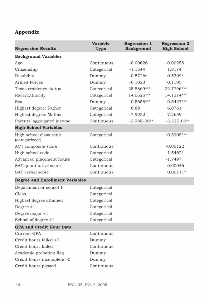
After the initial regression including student backgroundinformation, each subsequent regression retains the previousset of variables and adds the new group of variables. As a re-sult, variables that were predictive in the earlier regressionsshifted in predictive power and significance as new informationwas included. The results of the series of regressions, includingthe data mining regression, appear on a table in the Appendix.The table shows the raw regression coefficient and the p-valueof those variables with a significance level of 0.05 or lower.

Demographic Data

The demographic variables entered into the first regressionincluded age, race/ethnicity, gender, disability, service in the

Research Models

and Results


Table 3

Frequencies of Selected Variables

Total Number Default

Value Number Percent (%) Defaulted Rate (%)

All 23,407 100.0 1,306 5.58

GenderMale 11,749 50.2 810 6.89Female 11,657 49.8 496 4.25

Race/EthnicityAfrican American 1,378 5.9 169 12.26Hispanic 4,383 18.7 319 7.28Native American 118 0.5 8 6.78Asian American 1,981 8.5 94 4.75White/non-Hispanic 15,536 66.4 716 4.61Missing values 9 0.0 0 0.00Other 2 0.0 0 0.00

Current Age20-24 2694 11.5 270 10.0240+ 1765 7.5 125 7.0825-29 9555 40.8 499 5.2230-39 9393 40.1 412 4.39

Texas Residency StatusTexas resident 18,388 78.6 1,155 6.28Non-Texas resident 3,155 13.5 87 2.76Foreign resident 5 0.0 0 0.00Not provided/missing 1,859 7.9 64 3.44

Highest Degree: FatherHigh school diploma 281 1.2 23 8.19Baccalaureate 215 0.9 15 6.98Associate degree 1,942 8.3 118 6.08Certification of completion 4,682 20.0 229 4.89Missing values 16,287 69.6 921 5.65

Highest Degree: MotherHigh school diploma 305 1.3 24 7.87Baccalaureate 119 0.5 8 6.72Associate degree 2,744 11.7 156 5.69Certification of completion 4,003 17.1 209 5.22Missing values 16,236 69.4 909 5.60

High School Class Rank-Categorized25.01 - 50.00 Percent 1,092 4.7 114 10.44Missing Values 30 0.1 3 10.000.01 - 25.00 percent 336 1.4 32 9.5250.01 - 60.00 percent 863 3.7 78 9.0460.01 - 70.00 percent 1,331 5.7 98 7.3670.01 - 80.00 percent 2,151 9.2 149 6.9380.01 - 90.00 percent 3,542 15.1 216 6.1090.01 - 100.00 percent 5,778 24.7 256 4.43Unknown 8,284 35.4 360 4.35

Highest Degree:borrowerHigh school diploma 5,058 21.6 801 15.84Special professional 16 0.1 1 6.25Baccalaureate 11,592 49.5 397 3.42Masters degree 4,392 18.8 70 1.59Doctoral degree 2,349 10.0 37 1.58

Note: Unless otherwise indicated, the categories are sorted from highest to lowest loan default rate.

36 VOL. 35, NO. 2, 2005

Table 3 (cont’d.)




Highest Class LevelFreshman 855 3.7 186 21.75Sophomore 988 4.2 154 15.59Junior 1,165 5.0 154 13.22Senior 12,916 55.2 647 5.01Doctoral 1,673 7.1 55 3.29Masters 4,274 18.3 91 2.13Law School 1,527 6.5 19 1.24Professional 8 0.0 0 0.00Missing Values 1 0.0 0 0.00

School of Degree #1No Degree Attained 6067 25.9 857 14.13Social Work 179 0.8 10 5.59Fine Arts 565 2.4 23 4.07Liberal Arts 4385 18.7 171 3.90Education 840 3.6 29 3.45Communication 1456 6.2 40 2.75Business Administration 1372 5.9 33 2.41Natural Sciences 1656 7.1 39 2.36Not provided 393 1.7 8 2.04Graduate School 2910 12.4 59 2.03Engineering 1175 5.0 22 1.87Law School 959 4.1 7 0.73Graduate Business 1219 5.2 8 0.66Nursing 231 1.0 0 0.00

Cumulative College GPA0.00 - 0.99 372 1.6 86 23.121.00 - 1.99 2,085 8.9 391 18.752.00 - 2.49 3,374 14.4 320 9.482.50 - 2.99 4,515 19.3 213 4.72Unknown 1,830 7.8 60 3.283.00 - 3.49 5,150 22.0 120 2.333.50 - 4.00 6,081 26.0 116 1.91

Credit Hours Failed FlagYes: Credit hours failed > 0 8,170 34.9 944 11.55No: Credit hours failed = 0 15,237 65.1 362 2.38

Financial Need LevelIndependent-single 2,909 12.4 252 8.66Zero parental contribution 2,620 11.2 217 8.28Parental contribution: $1-$3000 1,810 7.7 128 7.07Independent-married 1,327 5.7 82 6.18Parental contribution: > $3000 7,447 31.8 428 5.75Z-Missing values 1,890 8.1 98 5.19Graduate 4,566 19.5 93 2.04Graduate-married 838 3.6 8 0.95

Dependent/Independent StatusDependent 12,406 53.0 798 6.43Independent 9,805 41.9 449 4.58Missing values 1,196 5.1 59 4.93

Note: Unless otherwise indicated, the categories are sorted from highest to lowest loan default rate.


armed forces, citizenship, Texas residency status, the highestdegree attained by the father and mother, and parents’ aggre-gated income. The initial regression showed that three variableswere significant at the p = 0.001 level: race/ethnicity, gender,and Texas residency status. Of the different racial/ethnic cat-egories, Blacks and Hispanics were more likely to default thanWhites and Asians. This finding is supported by several otherstudies (Wilms, Moore & Bolus, 1987; Knapp & Seaks, 1992;Dynarksy, 1994; Flint, 1994, 1997; Volkwein & Szelest; 1995;Woo, 2002). In this study, men were more likely to default thanwomen. This result is also upheld in some prior studies (Flint,1994, 1997; Woo, 2002). Texas residents were more likely todefault than non-Texas residents.

Of other student characteristics, the disabilities flag wassignificant at the p = 0.05 level, but this variable had 60% miss-ing data and a low number of students with disabilities. Thesignificance of the parents’ aggregated income variable indicatedthat students whose parents have higher incomes are less likelyto default. This result has been found in previous default stud-ies (Wilms, Moore & Bolus, 1987; Knapp & Seaks, 1992;Dynarksy, 1994; Woo, 2002). Of the background variables, onlyrace/ethnicity, gender, and parents’ income remained statisti-cally significant as other groups of variables were added to theregression.

The general result of this regression implies that minor-ity students, particularly Blacks and Hispanics, are at a higherrisk of default. In addition, students coming from families withlower incomes are also at higher risk. These students mightbenefit from increased attention from UT Austin in the form ofinterventions that help students integrate into the campus com-munity and meet the cost of college education.



Net Guarantee Amount (in order of increasing net guarantee amount)$1-1,500 3,316 14.2 221 6.66$1,501-3,000 7,737 33.1 523 6.76$3,001-4,500 4,045 17.3 233 5.76$4,501-6,000 5,325 22.8 228 4.28$6,001-7,500 996 4.3 28 2.81$7,501-9,000 1,134 4.8 22 1.94$9,001-10,500 440 1.9 17 3.86$10,501-12,000 90 0.4 0 0.00$12,001-15,000 134 0.6 9 6.72$15,001-18,000 50 0.2 2 4.00$18,001-21,000 34 0.1 4 11.76$21,001-24000 12 0.1 5 41.67> $24,000 93 0.4 14 15.05

Table 3 (cont’d.)


38 VOL. 35, NO. 2, 2005

High School Data

The second grouping of data included variables capturing stu-dents’ high school performance. Unfortunately, high school GPAwas not included in the data set for unknown reasons, but highschool rank, advanced placement hours, and ACT and SAT testscores were in the data set. Of the high school variables, highschool rank, high school College Board code, and the SAT ver-bal score emerged as statistically significant. Students with lowerhigh school rank were more likely to default. Interestingly, ahigher SAT verbal score was weakly linked to loan default, aresult that remained constant across all regressions. Thecounterintuitive results of the SAT verbal score are not easilyexplained. In this author’s experience of retention modeling, theSAT verbal score is often more strongly correlated to studentpersistence than either the SAT combined score or SAT mathscore. While the dependent variable of this model is loan de-fault, the result remains puzzling. Neither the SAT math norSAT combined score entered as significant explanatory variables.

High school College Board code was a categorical vari-able that was classified. This means that the single variablecontained the average loan default rates of all high schools thathad more than 12 students attending UT Austin in the model-ing file. Generally, high school code can be interpreted as a geo-graphic and academic variable, identifying high schools acrossTexas and the rest of the country with students who were morelikely than average to default.

High school performance and completion have emergedas significant in several cross-institutional studies (Wilms, Moore& Bolus, 1987; Dynarski, 1994; Flint, 1994; Woo, 2002). Allstudies imply that high school completion and a better highschool performance are linked to lower loan default rates. Thisregression reaffirmed these results, although the particular mixof predictive variables appeared rather unintuitive. For example,it is possible that certain high schools may tend toward stronggrade inflation or other characteristics that place their studentsat increased risk. In the absence of additional information, UTAustin could focus on high school rank as an indicator of even-tual loan default.

Degree Completion and GPA Data

Degree completion data emerge as the strongest predictors ofloan default status. The most important variables are the high-est degree attained, the highest class level reached before leav-ing UT Austin, and the school at UT Austin from which the stu-dent earned the degree. These variables overlap and have somedegree of intercorrelation, but were still independent enough tobe entered into the regressions together as a group. The datademonstrate that students who earned graduate degrees werethe least likely to default. The average default rate of studentswho received a high school diploma (as opposed to a college

Interestingly, a higher

SAT verbal score was

weakly linked to loan

default, a result that

remained constant

across all

regressions.


degree) was 15.8%. Borrowers who attained a bachelor’s degreehad an average loan default rate of 3.4%, and master’s and doc-toral degree recipients had an average default rate of 1.6% whenrounded to the nearest tenth.

Of the students who did not receive a degree, those wholeft as freshmen were most likely to default (average default rateof 21.75%), followed by sophomores (15.59%) and juniors(13.22%). Students who left as seniors had an average defaultrate of 5.01%, close to the sample average of 5.58%, while stu-dents with graduate or professional degrees had below averagedefault rates. Students who did not receive a degree were morelikely to default than any other group of students. These resultsare echoed by previous studies that find degree completion oneof the strongest predictors of loan default (Wilms, Moore & Bo-lus, 1987; Knapp & Seaks, 1992; Dynarksy, 1994; Flint, 1997;Volkwein & Szelest; 1995; Texas Guaranteed, 1998b; Woo, 2002,Gladieux & Perna, 2005).

Once degree information is added to the model, severalvariables either gain or lose statistical significance. This hap-pens as the new variables in the model either substitute for, oramplify the effects captured by the other variables. Age was nota statistically significant variable in the first two regressions,but enters the model once degree information is added to themodel. The coefficient implies that students who are older aremore likely to default, which contradicts findings that studentswho drop out early, as freshmen, are most likely to default.

One possible interpretation of this result is that the co-efficients for the degree variables give too much weight to youngerstudents and that this is compensated for by adding to the de-fault risk of older students through the age variable. Also, olderstudents tend to have other obligations besides paying for col-lege, and these other expenses may account for their higherdefault tendencies. Table 3 shows that the relationship of ageand loan default is not linear, but that students between theages of 20-24 and over 40 have higher loan default rates thanborrowers in their late twenties and thirties. Similarly, high schoolrank, high school code, and the Texas residency variable losestatistical significance when degree information is included inthe regression, and remain insignificant in subsequent analyses.

This regression offered important information for UTAustin in terms of potential student interventions. Student per-sistence and degree completion emerged as the main variablesin this regression. Freshmen persistence, in particular, wasimportant in predicting eventual loan repayment. Enhancingthe first-year experience and targeting first-year retention ratesappears a worthwhile effort for UT Austin. Based on this data, itwould seem that any intervention that helps students persistand succeed in college would substantially lower their risk ofloan default.

It would seem thatany intervention thathelps studentspersist and succeedin college wouldsubstantially lowertheir risk of loandefault.

40 VOL. 35, NO. 2, 2005

College GPA, Hours Failed, Hours Incomplete, Transfer Hours,

and Graduate Studies Flag

The data set also contained the students’ final cumulative col-lege GPA, the number of hours a student had failed, the num-ber of hours for which the students had received an incompletegrade, and number of hours the student had passed. An addi-tional flag indicated that the student had been placed on aca-demic probation. Of these variables, all but two emerged as highlysignificant. College GPA was one of the strongest predictors.Students leaving UT Austin with a higher college GPA were lesslikely to default. Students who had failed any credit hours incollege were more likely to default, as were students who hadincomplete grades on their academic record. Neither the aca-demic probation flag nor the number of credit hours passedwas significant.

The inclusion of this level of detail about the student’sacademic performance is unique to this data set and under-scores the effects of student persistence and academic successon future student loan defaults. In this study, students whohad failed any credit hours had an average loan default rate of11.6% compared with an average default rate of 2.38% for stu-dents who had no failed credit hours on their record. This infor-mation gives UT Austin another point of early intervention byfocusing on students who had any failed credit hours on theirrecord, especially early in their enrollment.

Transfer Hours and Graduate Studies Flag

The presence of transfer credit hours was negatively related toloan default, but a higher transfer GPA had a positive effect onloan default. This result may be due to interactions betweenvariables. Single variable analyses show that students with ahigher transfer GPA are less likely to default. While variablesthat were too highly correlated were omitted from the analysis,this threshold was set rather high (at a Pearson’s correlationcoefficient of 0.80) and did not preclude some unexpected vari-able interaction. Completing graduate credit hours was not sig-nificant in this regression but gained a low level of significancewhen student income variables were added.

Adding transfer hours and a graduate studies flag al-lowed UT Austin to assess the risk level for transfer studentsand graduate students. The general results upheld that aca-demically strong students and students who complete theirundergraduate degree by enrolling in graduate hours are at alower risk for loan default.

Income and Financial Aid Variables

Of the available income and financial aid data, the amount oftaxes paid was highly significant when submitted in combina-tion with the aggregated income variable. When we eliminatedthe amount of taxes paid from the model, aggregated income

The inclusion of this

level of detail about

the student’s

academic

performance is

unique to this data

set and underscores

the effects of student

persistence and

academic success

on future student

loan defaults.


became highly significant. This indicates that borrowers pay-ing taxes—who are also the borrowers with higher incomes—are less likely to default. Students who are employed and havehigher incomes have been shown to be at a lesser risk of loandefault in other studies (Choy, 2000; Woo, 2002; Choy & Li,2005). Other income variables tested in the model included fi-nancial need, status as financially dependent student, adjustedgross income, and last loan payment amount collected. None ofthese variables were statistically significant in this regression.

Data Mining Model

The group of variables most highly correlated to student loandefault were submitted to the data mining modeling process.This group included 38 variables with correlation coefficientsranging from 0.23 to 0.03. Only variables with a minimum per-centage of missing values were considered for this model.

The final model combined the demographic, degreecompletion, credit hour, and financial variables. Race/ethnicityand gender remained highly significant and accounted for ap-proximately 20% of the variation in default behavior explainedby the model. The highest educational degree attained, academicgrade level, and school of enrollment variables provided a de-tailed degree-completion and persistence profile. Taken together,the degree completion variables accounted for more than 50%of the variation in default behavior explained by the model(see Figure). The number of credit hours failed underlined theimportance of academic success and explained another 20% of

Figure

Relative Strength of Model Variables

The percentages are calculated as the proportion of total variance of the model explained by a particular variable,

as measured by the absolute value of the t-statistic for that variable.

Highest degree attained (26.9%)

Credit hours failed (21.1%)

Class level (7.1%)

Race/ethnicity (12.6%)

Gender (5.9%)

School of degree #1 (12.3%)

Dependent/Independent Status (14.2%)

26.9%

14.2%

12.3%

5.9%

12.6%

7.1%

21.1%

42 VOL. 35, NO. 2, 2005

borrower behavior, while the financial dependency status vari-able added a financial aid component to the model. This modelwas able to predict correctly 76% of the students as defaultersor repayers by the assigned model score. The results of thismodel echo those of the previous regressions, though in a moreefficient model including only seven highly significant variables.

This model provided UT Austin with a succinct profile ofpotential defaulters that suggested many possible points of in-tervention spanning a student’s educational experience. Stu-dent socioeconomic background and possible first-generationstudent status might be proxied by the race/ethnicity variable.Academic grade level and the credit hours failed emphasizedthe importance of first-year retention, and the highest degreeattained demonstrated the importance of continued studentsuccess at all grade levels.

Student loan default can be predicted with limited success fromstudent background variables alone. Both gender and race/ethnicity remain strong predictors throughout all regressions.Based on parents’ income variables, students from a higher so-cioeconomic background are less likely to default. High schoolperformance is important, but only in the absence of collegeand degree information.

Degree completion and academic success are the stron-gest predictors of future loan default. Students who completedtheir degree and have a high college GPA were least likely todefault. The earlier a student withdrew from UT Austin, the stron-ger the likelihood of default. Academic failure—often a precur-sor to academic withdrawal—also had a strong effect on futuredefault. Failing any credit hours at all increased the possibilityof default from 2.38% to 11.55%. These results point to theopportunity of influencing the loan default rate by focusing onstudent persistence and success at the time a student enrollsat UT Austin.

Of the financial variables, only the amount of taxes paidhad any statistically significant influence on default behavior,which suggests that borrowers with higher incomes after leav-ing school were less likely to default. Other studies with morecomplete financial data have shown that post-enrollment em-ployment status and higher levels of income lower the likeli-hood of default and keep the borrower’s debt burden at accept-able levels of default (Hansen & Rhodes, 1988; Dynarksy, 1994;Flint, 1997; Volkwein & Szelest; 1995; Choy, 2000; Woo, 2002;Choy & Li, 2005). One way UT Austin could influence studentemployment is through its alumni network and career counsel-ing.

The data mining model summarized the most salientcharacteristics that affected student loan default. The goal ofthe data mining model was to predict future loan defaulters andassign a risk score to each borrower indicating his or her likeli-

Profile of Student

Loan Default


hood of default. An additional goal was to find variables thatwould allow either the loan guarantor or the institution to iden-tify at-risk borrowers as early as possible and take interventionmeasures to help prevent student loan default. The profile re-sulting from this model emphasized student background char-acteristics, degree completion, and the importance of academicsuccess. Because of its comprehensive nature, this was the modelbest suited for investigating possible student interventions.

This study is unusual in that it originated with a student loanguarantor and an institution. The base for this model was co-horts of borrowers who entered loan repayment from 1996 to1999, and included students from all academic levels and disci-plines. While this group of borrowers reflected the loan defaultissue from the point of view of the loan guarantor, it provided anincomplete picture to the academic institution. The focus onloan default cohorts limited the ability to append complete aca-demic data to all student records and resulted in a data struc-ture that contained many missing values, precluding a trulycomprehensive analysis. Nevertheless, the models were able topredict correctly 70% - 79% of the students as defaulters orrepayers based on the risk scores derived from the models.

Despite the data limitations, the data show two factorsas strongly influencing student loan defaults: student persis-tence and degree completion. This result provides UT Austinwith powerful information about the possibilities of lowering theiroverall loan default rate and preventing individual loan defaults.Goals for increasing student retention and program completionare well within the scope of UT Austin and can be affected withtargeted interventions at the student level. While these inter-ventions will never eliminate default entirely, helping studentsto succeed will reduce the greatest risk of loan default.

It is possible to take these results one step further anduse them to enhance the institution’s default reduction efforts.Overall, the estimated models reflect broad trends that empha-size student success as a key factor in reducing defaults. Be-cause the data included students from all academic levels andprograms, the model was able to identify the effects of addi-tional years of schooling on loan default rates. Based on theresults, it appears that a more direct focus by UT Austin onstudent retention from freshmen to sophomore year might helpthe institution to further refine its default prevention efforts.

To achieve this, UT Austin could use the same data min-ing approach to estimate a freshmen-to-sophomore retentionmodel using all available data for first-year entering students.This model would have the advantage of focusing on an aca-demic cohort rather than a loan default cohort that combinesacademic years and degrees. The data would be more immedi-ate and the time needed to implement effective policies wouldbe shortened by years. Furthermore, because the model would

Implications of

the Models

44 VOL. 35, NO. 2, 2005

be based on more complete and timely data, the predictive fac-tors of this model would signal possible academic interventionstailored to freshmen—the most at-risk group.

In the aftermath of the predictive data mining model, UT Austinhas both investigated aspects of student retention and soughtways to use the model to plan and implement student interven-tions, particularly those aimed at students who fail at least oneacademic class. Several university offices were involved in theseefforts. Follow-up information obtained from UT Austin’s aca-demic enrichment services (AES) showed that students are mostlikely to drop out of college during their junior year. In mostcases, juniors with low GPAs typically received their first failinggrade as early as their first semester. In an effort to boost reten-tion and decrease student loan default, the office of studentfinancial services (OSFS) recently initiated the “Pathway toProgress” (PTP) program. The PTP program combines the effortsof the OSFS, AES, and academic advisors to provide immediateand comprehensive support to freshmen who received at leastone failing grade during their first semester. This three-pointapproach is intended to help reduce financial or academic bar-riers that may have contributed to the student failing one ormore courses.

The PTP program identified approximately 300 aid re-cipients and divided them into three groups. The first groupconsisted of students who failed more than one course. Thesestudents were required to meet with a representative from OSFS,AES, and an academic advisor. The second group containedFederal Pell Grant recipients with one failing grade. These stu-dents met only with a financial aid counselor and an academicadvisor. The final group contained non-Pell-eligible students withone failing grade. They were only required to meet with a finan-cial aid counselor. In all cases, the student completed a PTPform where they reported what factors contributed to their fail-ing grade and what they intended to do to improve their aca-demic performance. The students were counseled on using thefull extent of services provided by the university.

UT Austin initiated this program late in the spring se-mester of 2004. Because PTP is designed to be most effectivewhen students are contacted early in spring, the effects are ex-pected to be minimal for fall 2004 freshmen. However, a struc-ture is now in place for productive fall and spring programs. Weexpect that PTP will expand beyond first-time freshmen to in-clude all grade levels, and anticipate that this program will greatlyassist students in obtaining their degrees, which may signifi-cantly decrease the likelihood of defaults.

Continued Efforts


References

Berkner, L. (2000). Trends in undergraduate borrowing: Federal student loans in 1989-90, 1992-93 and 1995-96.

(NCES 2000-151). Washington, DC: National Center for Education Statistics, U.S. Department of Education.

Choy, S. (2000). Debt burden four years after college. (NCES 2000-188). Washington, DC: National Center forEducation Statistics, U.S. Department of Education.

Choy, S. & Li, X. (2005). Debt burden: A comparison of 1992-93 and 1999-2000 bachelor’s degree recipients a

year after graduating. (NCES 2005-170). Washington, DC: National Center for Education Statistics, U.S. Depart-ment of Education.

Clinedinst, M. E.; Cunningham, A. F & Merisotis, J. P. (2003). Characteristics of undergraduate borrowers: 1999-

2000. (NCES 2003-155). Washington, DC: National Center for Education Statistics, U.S. Department of Educa-tion.

College Board, (2002). Trends in student aid 2002. Washington, DC. Author.

College Board (2003). Trends in student aid 2003. Washington, DC. Author.

Dynarski, M. (1994). Who defaults on student loans? Findings from the National Postsecondary Student AidStudy. Economics of Education Review, 13(1), 55-68.

Flint, T. A. (1994). The federal student loan default cohort: A case study. Journal of Student Financial Aid, 24(1),13-30.

Flint, T. A. (1997). Predicting student loan defaults. Journal of Higher Education, 68(3), 322-354.

Gladieux, L. & Perna, L. (2005). Borrowers who drop out: A neglected aspect of the college student loan trend.(National Center Report #05-2) The National Center for Public Policy and Higher Education. Online. Available:[http://www.highereducation.org/reports/borrowing/index.shtml]

Greiner, K. (1996). How much student loan debt is too much? The Journal of Student Financial Aid, 26(1), 7-16.

Hansen, W. L. & Rhodes, M. S. (1988). Student debt crisis: Are students incurring excessive debt? Economics in

Education Review, 7(1), 101-112.

Hosmer, D. & Lemeshow, S. (2000). Applied Logistic Regression. John Wiley & Sons, Inc.: New York.

Knapp, L. G. & Seaks, T. G. (1992) An analysis of the probability of loan default on federally guaranteed studentloans. The Review of Economics and Statistics, 74(3), 404-411.

Lein. L., Rickards, R., & Webster, J. (1993). Student loan defaulters compared with repayers: A Texas casestudy. Journal of Student Financial Aid, 23(1), 29-39.

Steiner, M. & Teszler, N. (2003). The characteristics associated with student loan default at Texas A&M Univer-sity. Austin, TX. Texas Guaranteed Student Loan Corporation.

Texas Guaranteed (1998a). Education on the installment plan: The rise of student loan indebtedness in Texas.Online. Available: [http://www.tgslc.org/publications/reports/indebtedness/]

Texas Guaranteed (1998b). Student loan defaults in Texas: Yesterday, today and tomorrow. Online. Available:[http://www.tgslc.org/publications/reports/defaults_texas/]

U.S. Department of Education (16 September 2003). Student loan default rates lowest ever. Online. Available:[http://www.ed.gov/news/pressreleases/2003/09/09162003.html]

Volkwein, J. F. & Cabrera, A. F. (1998). Who defaults on student loans?: The effects of race, class, and gender onborrower behavior in Condemning Students to Debt: College Loans and Public Policy. Fossey, R. & Bateman, M.Eds. New York: Teachers College Press.

Volkwein, J. F. & Szelest, B. P. (1995). Individual and campus characteristics associated with student loandefault. Research in Higher Education, 36(1), 41-72.

Wilms, W. W., Moore, R. W. & Bolus, R. E. (1987). Whose fault is default? A study of the impact of studentcharacteristics and institutional practices on Guaranteed Student Loan default rates in California. Educational

Evaluation and Policy Analysis, 9(1), 41-54.

Woo, J. (2002). Factors affecting the probability of default: Student loans in California. Journal of Student Finan-

cial Aid, 32(2), 5-23.

46 VOL. 35, NO. 2, 2005

Appendix

Variable Regression 1 Regression 2

Regression Results Type Background High School

Background Variables

Age Continuous -0.00626 -0.00258

Citizenship Categorical -1.1544 1.8174

Disability Dummy 0.5726* 0.5309*

Armed Forces Dummy -0.1023 -0.1195

Texas residency status Categorical 25.5869*** 22.7796***

Race/Ethnicity Categorical 14.0626*** 14.1314***

Sex Dummy 0.5658*** 0.5427***

Highest degree: Father Categorical 6.89 6.0761

Highest degree: Mother Categorical -7.9922 -7.2659

Parents’ aggregated income Continuous -2.98E-06** -3.32E-06**

High School Variables

High school class rank Categorical 10.5905***(categorizeda)

ACT composite score Continuous -0.00122

High school code Categorical 1.5462*

Advanced placement hours Categorical -1.7497

SAT quantitative score Continuous -0.00046

SAT verbal score Continuous 0.00111*

Degree and Enrollment Variables

Department or school 1 Categorical

Class Categorical

Highest degree attained Categorical

Degree #1 Categorical

Degree major #1 Categorical

School of degree #1 Categorical

GPA and Credit Hour Data

Current GPA Continuous

Credit hours failed >0 Dummy

Credit hours failed Continuous

Academic probation flag Dummy

Credit hours incomplete >0 Dummy

Credit hours passed Continuous


Regression 3 Regression 4 Regression 5 Regression 6 Regression 7

Degree Info GPA/Hours Transfer/Grad Financial Data Mining

Background Variables

0.0488*** 0.0526*** 0.0503*** 0.0554***

0.9951 2.4216 3.663 3.23

0.1141 0.1592 0.1747 0.1553

-0.2093 -0.2156 -0.224 -0.2301

5.5641 2.4994 6.0384 5.9163

12.0747*** 9.3502*** 9.1119*** 9.1493*** 10.15089***

0.4483*** 0.3262*** 0.3066*** 0.2971*** 0.2293**

-3.8356 -5.1905 -5.3847 -4.6895

-5.8318 -8.2483 -7.9245 -8.1708

-6.22E-06*** -6.7E-06*** -6.42E-06*** -5.3E-06**

High School Variables

0.6001 -0.3213 -0.1855 -0.0384

0.00181 0.00265 0.00265 0.00307

0.7976 0.7242 0.733 0.6582

-4.256 -8.4354 -7.8677 -8.1886

0.0006 0.0007 0.000807 0.000795

0.00114* 0.00142** 0.00112* 0.00111*

Degree and Enrollment Variables

7.4317*** 4.4845* 6.107** 5.6152**

3.4626*** 2.8931** 1.8685* 1.6348 2.5715**

13.02*** 9.8868*** 10.4094*** 10.1733*** 11.0232***

5.7079 5.2174 6.1027 5.8365

0.3798 0.3335 0.3159 0.2347

13.8177** 11.7674** 13.2788** 12.1557** 23.7350***

GPA and Credit Hour Data

-0.3523*** -0.391*** -0.3899***

0.5653*** 0.5857*** 0.5754***

0.0369***

0.0831 0.0674 0.0652

1.0785*** 0.9591*** 0.9307****

0.00164 0.00239* 0.00187

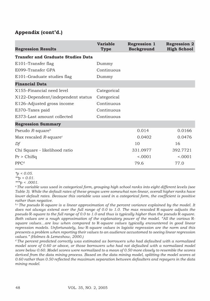
48 VOL. 35, NO. 2, 2005

*p < 0.05.

**p < 0.01.

***p < .0001.a The variable was used in categorical form, grouping high school ranks into eight different levels (see

Table 3). While the default rates of these groups were somewhat non-linear, overall higher ranks have

lower default rates. Because this variable was used in a categorical form, the coefficient is positive

rather than negative.b,c The pseudo R-square is a linear approximation of the percent variance explained by the model. It

does not always extend over the full range of 0.0 to 1.0. The max rescaled R-square adjusts the

pseudo R-square to the full range of 0.0 to 1.0 and thus is typically higher than the pseudo R-square.

Both values are a rough approximation of the explanatory power of the model. “All the various R-

square values…are low when compared to R-square values typically encountered in good linear

regression models. Unfortunately, low R-square values in logistic regression are the norm and this

presents a problem when reporting their values to an audience accustomed to seeing linear regression

values.” (Holmes & Lemeshow, 2000.)d The percent predicted correctly was estimated as borrowers who had defaulted with a normalized

model score of 0.60 or above, or those borrowers who had not defaulted with a normalized model

score below 0.60. Model scores were normalized to a mean of 0.50 more closely to resemble the scores

derived from the data mining process. Based on the data mining model, splitting the model scores at

0.60 rather than 0.50 reflected the maximum separation between defaulters and repayers in the data

mining model.

Appendix (cont’d.)

Variable Regression 1 Regression 2

Regression Results Type Background High School

Transfer and Graduate Studies Data

E101–Transfer flag Dummy

E099–Transfer GPA Continuous

E101–Graduate studies flag Dummy

Financial Data

X155–Financial need level Categorical

X122–Dependent/independent status Categorical

E126–Adjusted gross income Continuous

E370–Taxes paid Continuous

E373–Last amount collected Continuous

Regression Summary

Pseudo R-squareb 0.014 0.0166

Max rescaled R-squarec 0.0402 0.0476

Df 10 16

Chi Square - likelihood ratio 331.0977 392.7721

Pr > ChiSq <.0001 <.0001

PPCd 79.6 77.0


Regression 3 Regression 4 Regression 5 Regression 6 Regression 7

Degree Info GPA/Hours Transfer/Grad Financial Data Mining

Transfer and Graduate Studies Data

-0.5026*** -0.5234***

0.0871** 0.1186***

0.2468 0.3309*

Financial Data

1.5797

-8.4999 -29.6117***

-0.00000395

-0.00012*

-0.00003

Regression Summary

0.0588 0.0676 0.0693 0.0704 0.0601

0.1682 0.1931 0.1981 0.2013 0.1719

22 27 30 35 7

1419.6442 1637.3353 1680.9696 1708.8295 1451.1909

<.0001 <.0001 <.0001 <.0001 <.0001

73.3 70.6 70.7 70.5 75.8

Predicting Student Loan Default for the University of ... · PDF filestudent loan default is a serious issue for borrowers, schools, lenders, and guarantors. Prior studies on the causes

Documents