Predicting RF Path Loss in Forests Using Satellite ...

Predicting RF Path Loss in Forests Using Satellite

Measurements of Vegetation Indices

by

Sujuan Jiang

A thesis submitted in partial fulfillment of the requirements for the degree of

Master of Science

Department of Computing Science

University of Alberta

c© Sujuan Jiang, 2015

Abstract

In this thesis, we propose a novel method for predicting the value of the radio

frequency (RF) path loss exponent (PLE) from satellite remote sensing obser-

vations. The value of the PLE is required when designing wireless sensor net-

works for environmental monitoring. By taking field path loss measurements

in single cells and extracting values of vegetation indices (VIs) from satellite

data, we successfully build correlation models between PLE and VIs of differ-

ent dates. We also characterize the composite correlation of all data from all

the filed measurements, which covers the whole in-leaf phrase in forests. The

correlations are strong (R2 > 0.77) and exhibit high statistical significance

(p < 0.01). It enables us to characterize and predict the RF propagation envi-

ronment in forested areas without the need for field measurements, given that

satellite data are available any location on Earth. We also propose a method

of predicting missing high-resolution 30m x 30m Landsat 8 data required by

our method from lower-resolution 250m x 250m MODIS observations that are

not as easily degraded. Finally, we use the composite correlation model to

predict path loss across multiple cells. A weighted sum method is applied to

calculate the overall PLE value for a path across multiple cells. We compare

the predicted RSSI values against actual field data. The result shows that the

predicted RSSI data are very close to the field data with error less than 5%.

ii

Acknowledgements

First of all, I would like to express my deepest gratitude to my supervisor

Prof. Mike H. MacGregor. He provided me many learning opportunities

during my graduate study. His outstanding guidance, continuous support,

and useful feedback is an invaluable asset to my research work. It is such a

pleasure to work with this awesome professor. Taking field trips to Mandy

Lake with him has always been a wonderful experience.

In addition, I am thankful to my committee members, Prof. Janelle Harms

and Arturo Sanchez-Azofeifa, for taking their time to read my thesis and be

involved in my defense.

Moreover, I would like to thank Dr. Carlos Portillo-Quintero for his train-

ing me on processing the satellite data and providing useful feedback, and the

department of Earth and Atmospheric Sciences for allowing me to access their

resources. Without their help, this thesis would not have been completed.

Finally, I would like to thank my families and friends for their love and

support all my life.

iii

Table of Contents

1 Introduction 1

1.1 Motivation . . . . . . . . . . . . . . . . . . . . . . . . . . . . . 1

1.2 Contributions . . . . . . . . . . . . . . . . . . . . . . . . . . . 2

1.3 Organization . . . . . . . . . . . . . . . . . . . . . . . . . . . 4

2 Predicting Path Loss across Single Cells 5

2.1 Background . . . . . . . . . . . . . . . . . . . . . . . . . . . . 5

2.1.1 RF Propagation through Vegetation . . . . . . . . . . . 6

2.1.2 Satellite Data and Vegetation Indices . . . . . . . . . . 8

2.2 Methodology . . . . . . . . . . . . . . . . . . . . . . . . . . . 11

2.2.1 Determining K . . . . . . . . . . . . . . . . . . . . . . 12

2.2.2 Measuring RSSI . . . . . . . . . . . . . . . . . . . . . . 15

2.2.3 Predicting Missing VI Values . . . . . . . . . . . . . . 16

2.3 Field Measurements . . . . . . . . . . . . . . . . . . . . . . . . 17

2.4 Data Reduction . . . . . . . . . . . . . . . . . . . . . . . . . . 19

2.4.1 Measuring RSSI . . . . . . . . . . . . . . . . . . . . . . 19

2.4.2 Interpolating Missing VI Measurements . . . . . . . . . 20

2.5 Correlating α to VIs . . . . . . . . . . . . . . . . . . . . . . . 21

2.5.1 Correlating α to VIs for Each Trip . . . . . . . . . . . 21

2.5.2 The Composite Correlation Model . . . . . . . . . . . . 28

2.6 Results and Discussion . . . . . . . . . . . . . . . . . . . . . . 39

iv

3 Predicting Path Loss across Multiple Cells 42

3.1 Weighted Sum Model . . . . . . . . . . . . . . . . . . . . . . . 42

3.2 SensorCloud Data . . . . . . . . . . . . . . . . . . . . . . . . . 44

3.3 Multi-cell Path Loss Calculations . . . . . . . . . . . . . . . . 46

3.3.1 Calculating Path Loss Using the Correlation Model . . 46

3.3.2 Comparison between Predicted and Actual RSSI . . . . 49

3.4 Results and Discussion . . . . . . . . . . . . . . . . . . . . . . 49

4 Conclusions and Future Work 52

Bibliography 54

v

List of Tables

2.1 RSSI Measurements Used to Find K . . . . . . . . . . . . . . 14

2.2 RSSI (dB) of June to October in 2013 and 2014 . . . . . . . . 19

2.3 NDVI values of MODIS data from May to September of 2013 . 20

2.4 Actual and Predicted NDVI Values for August 24, 2013 . . . . 20

2.5 Predicted NDVI Values for July 23, 2013 . . . . . . . . . . . . 21

2.6 Cell Data of 2013 . . . . . . . . . . . . . . . . . . . . . . . . . 22

2.7 Cell Data of 2014 . . . . . . . . . . . . . . . . . . . . . . . . . 22

2.8 RSSI and z-values . . . . . . . . . . . . . . . . . . . . . . . . . 37

2.9 Suitability of Regression Models . . . . . . . . . . . . . . . . . 40

3.1 NDVI and α Values for Each Cell of the Testing Dates . . . . 48

3.2 Distances of Paths Across Each Cell . . . . . . . . . . . . . . . 48

3.3 Predicted and Actual RSSI Data from Each Sensor to the Ag-

gregator of September 25, 2013 . . . . . . . . . . . . . . . . . 50

3.4 Predicted and Actual RSSI Data from Each Sensor to the Ag-

gregator of June 8, 2014 . . . . . . . . . . . . . . . . . . . . . 50

vi

List of Figures

2.1 Green Plants’ Reflectance of Different Wavelengths . . . . . . 9

2.2 Landsat 8 Images (30m x 30m) . . . . . . . . . . . . . . . . . 10

2.3 Network Grid of Taking Signal Loss Measurements . . . . . . 11

2.4 RSSI in the Sparse Area . . . . . . . . . . . . . . . . . . . . . 14

2.5 RSSI in the Dense Area . . . . . . . . . . . . . . . . . . . . . 15

2.6 A Landsat 8 Image with Cloud Cover of 36% . . . . . . . . . . 16

2.7 Grid of Study Area . . . . . . . . . . . . . . . . . . . . . . . . 18

2.8 Grid of Pixels in Landsat 8 Image . . . . . . . . . . . . . . . . 18

2.9 Linear Fit of α vs. NDVI on July 23, 2013 . . . . . . . . . . . 23

2.10 Logarithmic Fit of α vs. NDVI on July 23, 2013 . . . . . . . . 23

2.11 Quadratic Fit of α vs. NDVI on July 23, 2013 . . . . . . . . . 24

2.12 Linear Fit of α vs. NDVI on August 24, 2013 . . . . . . . . . 24

2.13 Logarithmic Fit of α vs. NDVI on August 24, 2013 . . . . . . 25

2.14 Quadratic Fit of α vs. NDVI on August 24, 2013 . . . . . . . 25

2.15 Linear Fit of α vs. NDVI on June 7, 2014 . . . . . . . . . . . 26

2.16 Linear Fit of α vs. NDVI on June 22, 2014 . . . . . . . . . . . 26

2.17 Linear Fit of α vs. NDVI in October, 2013 . . . . . . . . . . . 27

2.18 NDVI and α Values from All Field Trips . . . . . . . . . . . . 28

2.19 An Outlier of All the Data Points . . . . . . . . . . . . . . . . 29

2.20 Linear Fit of α to VIs for Cell 2 Consisting of NDVI and α

Values from Different Dates . . . . . . . . . . . . . . . . . . . 30

vii







2.24 Linear Fit of α to VIs for Cell 4 . . . . . . . . . . . . . . . . 32

2.25 Linear Fit of α to VIs for Cell 4 after Removing the Outlier . 32




2.29 Linear Fit of α to VIs for Cell 8 and 9 after Removing the Outlier 34

2.30 Linear Fit of α vs. NDVI of the Composite Correlation . . . . 35

2.31 Logarithmic Fit of α vs. NDVI of the Composite Correlation . 36

2.32 Quadratic Fit of α vs. NDVI of the Composite Correlation . . 36

2.33 Normal Probability Plot . . . . . . . . . . . . . . . . . . . . . 38

2.34 Cumulative Periodogram . . . . . . . . . . . . . . . . . . . . . 39

3.1 A Path across Multiple Cells . . . . . . . . . . . . . . . . . . . 43

3.2 The WSDA Aggregator Deployed in the Field . . . . . . . . . 45

3.3 Deployment of Aggregator and Sensor Nodes . . . . . . . . . . 46

3.4 Actual RSSI Data Displayed on SensorCloud from Different

Sensors to the Aggregator . . . . . . . . . . . . . . . . . . . . 49

viii

Chapter 1

Introduction

1.1 Motivation

Wireless sensor networks (WSNs) have been very actively studied. There is a

rich literature of theoretical studies on the abstract properties of WSNs, and

algorithms for sensor coverage, sensor placement, relay placement, and base

station mobility [1, 2, 3, 4]. A key issue in designing and deploying WSNs

is the radio frequency (RF) propagation environment [5], largely because of

the limited energy budget at the wireless nodes. RF transmission, and to a

lesser extent, signal reception are the main consumers of energy in wireless

nodes. Thus, if we can predict the magnitude of RF signal loss in the area

to be covered by a WSN, we can develop power budgets for the links between

nodes, and estimate the lifetime of the network for given battery resources.

RF propagation through vegetation has been studied at least since the

1960’s [6]. One broad class of propagation models is empirical. These are

based on experimental measurements of received signal strength, converting

these data to attenuation, and regressing against distance. The current ITU-R

recommended model for predicting attenuation in vegetation is of this form [7].

The shortcoming of an empirical model is that it has no mechanistic link to the

properties of the vegetation in the area of interest. Model parameter values

are specific to the site [8] or species investigated [9]. The key parameter in

models for RF propagation through vegetation, such as the one recommended

1

by the ITU-R, is the path loss exponent (PLE).

In the thesis, we focus on RF propagation through vegetation. We propose

a novel method for predicting PLE values from Landsat 8 remote sensing obser-

vations. We use satellite data to determine the vegetation condition of a given

area of interest. A correlation model is built between PLE and Vegetation In-

dices (VIs) that represents vegetation densities. The satellite data we use are

available for any location on Earth, thus enabling characterization and predic-

tion of the RF propagation environment in forested area without the need for

field measurements. Also, we propose a novel way of predicting high-resolution

30m x 30m Landsat 8 data required by our method from lower-resolution 250m

x 250m MODIS observations that are not easily degraded. Such degradation

occurs relatively frequently when cloud cover or aerosols such as pollution or

sand storms degrade or significantly interfere with the high-resolution satellite

data we are using. Finally, based on the single-cell model, we predict path

loss through multiple cells. A heuristic weighted sum method is applied to

calculate the overall path loss exponent for a path crossing multiple cells, and

to predict the received signal strength indication (RSSI) along the path. We

compare the predicted RSSI against real field data.

1.2 Contributions

First, we propose a novel method for predicting PLE values from Landsat 8

remote-sensing observations. At the moment, our model is specific to aspen

boreal forests, which cover approximately 1.5 to 2.0 million square kilometres

in Canada alone. The method is generalizable to other forest types, and we

propose both broader coverage of boreal forests, and other vegetation types, as

future work. The satellite data we use are available for any location on Earth,

thus enabling characterization and prediction of the RF propagation environ-

ment in forested areas without the need for field measurements. As far as we

know, this is the first reported work that links remote sensing observations to

field predictions of RF loss.

A second contribution is that we also propose a novel way of predicting

high-resolution 30m x 30m Landsat 8 data required by our method from lower-

2

resolution 250m x 250m MODIS observations that are not as easily degraded.

Such degradation occurs relatively frequently when cloud cover or aerosols such

as pollution or sand storms degrade or significantly interfere with the high-

resolution satellite data we are using. We tested our proposal by comparing its

predictions to actual values for a date when the 30m x 30m data are available,

and the results show absolute errors of less than 5%.

In the end, we apply the single-cell correlation model between VI and PLE

to predict path loss across multiple cells. With available satellite data, we

have values of VI of all cells of the area of interest. By using the single-cell

model and VI values, we get values of PLE of each cell. We then calculate the

overall PLE for a path crossing multiple cells through a weighted sum method

based on the path’s distance in each cell. We compare the predicted RSSI data

against actual field data retrieved from SensorCloud that gathers RSSI from

deployed sensors in the area of interest. The result shows that the predicted

RSSI data are very close to the actual field data.

Our contributions are summarized as follows:

• Exploration and demonstration of a significant single-cell correlation be-

tween the value of the path loss exponent, and the values of remotely

sensed vegetation indices. The global availability of high-resolution 30m

x 30m satellite data for these indices thus enables RF path loss predic-

tions for WSNs anywhere in the world.

• Demonstration of a method for predicting high-resolution VI values from

lower-resolution 250m x 250m satellite data. This enables us to fill in

gaps in the temporal series of VI values when the satellite view of the

area of interest is obscured by clouds or aerosols.

• Application of a weighted sum method to get the overall path loss ex-

ponent for a path crossing multiple cells. The method enables us to

calculate the path loss between any two locations whose path crosses

multiple cells.

• Prediction of path loss across multiple cells based on the single-cell model

and the weight sum method. The predicted RSSI is compared against

3

the real data gathered from SensorCloud. This enables us to perform

network simulation tests without the need for field measurements.

1.3 Organization

The thesis is organized as follows. Chapter 2 reviews previous work of RF

propagation through vegetation and introduces relevant remote sensing obser-

vations including satellite data and vegetation indices. That is followed by our

experimental observations of predicting path loss across single cells for in-leaf

and out-of-leaf conditions at a site in Alberta, Canada. It also proposes a

method of predicting missing high-resolution data from lower-resolution satel-

lite observations. Chapter 3 presents our weighted sum method for predicting

path loss across multiple cells. The predicted RSSI data are compared against

real field data collected from SensorCloud. Chapter 4 presents conclusions and

future work.

4

Chapter 2

Predicting Path Loss across

Single Cells

In this chapter, we first present the background of RF propagation through

vegetation which motivates us to extend current work to heterogeneous forests

consisting of a mixture of species at varying densities. To measure the veg-

etation condition, we then introduce remote sensing observations of satellite

measurements and use vegetation indices to represent the intensity of green for

a given area of interst. Following that, we take field signal loss measurements

at Mandy Lake to get the path loss exponent, α, for each 30m x 30m area of

interest. VI values are also calculated from Landsat 8 images for the same cells

where we take the filed measurements. Finally, we characterize the correlation

model between VI and α of different dates as well as a composite correlation

model consisting of data points from all of our field trips. This is followed by

results and discussion.

2.1 Background

The free space path loss model assumes that during signal transmission, the

transmitter and receiver located in an empty open air area. It assumes that

the received signal only decreases with distance and is not affected by any

5

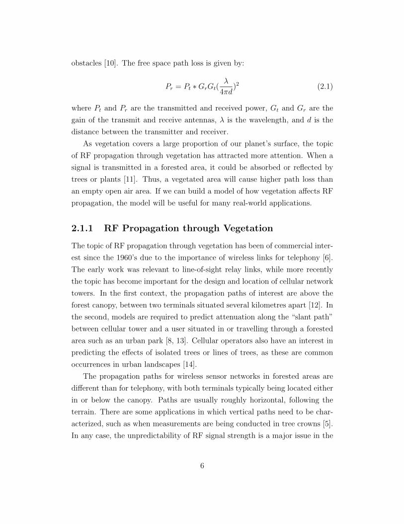
obstacles [10]. The free space path loss is given by:

Pr = Pt ∗GrGt(λ

4πd)2 (2.1)

where Pt and Pr are the transmitted and received power, Gt and Gr are the

gain of the transmit and receive antennas, λ is the wavelength, and d is the

distance between the transmitter and receiver.

As vegetation covers a large proportion of our planet’s surface, the topic

of RF propagation through vegetation has attracted more attention. When a

signal is transmitted in a forested area, it could be absorbed or reflected by

trees or plants [11]. Thus, a vegetated area will cause higher path loss than

an empty open air area. If we can build a model of how vegetation affects RF

propagation, the model will be useful for many real-world applications.

2.1.1 RF Propagation through Vegetation

The topic of RF propagation through vegetation has been of commercial inter-

est since the 1960’s due to the importance of wireless links for telephony [6].

The early work was relevant to line-of-sight relay links, while more recently

the topic has become important for the design and location of cellular network

towers. In the first context, the propagation paths of interest are above the

forest canopy, between two terminals situated several kilometres apart [12]. In

the second, models are required to predict attenuation along the “slant path”

between cellular tower and a user situated in or travelling through a forested

area such as an urban park [8, 13]. Cellular operators also have an interest in

predicting the effects of isolated trees or lines of trees, as these are common

occurrences in urban landscapes [14].

The propagation paths for wireless sensor networks in forested areas are

different than for telephony, with both terminals typically being located either

in or below the canopy. Paths are usually roughly horizontal, following the

terrain. There are some applications in which vertical paths need to be char-

acterized, such as when measurements are being conducted in tree crowns [5].

In any case, the unpredictability of RF signal strength is a major issue in the

6

design of WSNs [5]. Attenuation predictions are needed both statically as a

function of position at a given point in time, and dynamically as a function of

wind, weather, and vegetation condition (in-leaf or out-of-leaf).

Several mechanistic models of RF attenuation in vegetation have been de-

veloped [14, 15]. Below about 200 MHz, where the dimensions of the vegetation

are much smaller compared to the wavelength of the RF signal, a dissipative

slab model can be used [6]. Above this frequency, from 200 MHz to 2 GHz,

Cavalcante et al. proposed a four-layer slab model. This consists of a semi-

infinite ground plane supporting above it a trunk layer, canopy layer, and air

layer [6]. Models like these require numerical methods for solution, and depend

on the values for several parameters in each layer (permittivity, conductivity

and permeability). Their chief advantage over empirical models is that they

provide physical insight into wave characteristics and propagation modes [15].

The direction taken by the ITU-R in Recommendation P.833 [7] is to rec-

ommend an empirical model, rather than a mechanistic one. For a radio “slant

path” crossing the woodland, the attenuation loss, L, is :

L = AfBdC(θ + E)G (2.2)

where f is the radio frequency (MHz), d is the vegetation depth (m), θ is the

radio path elevation (degrees), and A,B,C,E, and G are empirically evaluated

parameters.

Common empirical models such as that recommended by the ITU-R predict

an exponential decrease in signal strength with both distance and frequency [9,

14]. The ITU-R Recommendation is a good starting point for the general form

of empirical predictions, but in itself is not sufficient for WSN design, directed

as it is towards paths that traverse the forest canopy, rather than tree trunks

and understory vegetation [16]. The parameter values in the Recommendation

are also of limited applicability, as they are tied to specific species of trees

that may or may not be present in a given area of interest. In addition,

the parameter values given in the Recommendation are for a single species

at a particular density. There is no guidance in the Recommendation for

sites consisting of a mixture of species of varying densities, and of course sites

7

consisting of other tree or plant species are not addressed at all.

Our goal in the present work is to extend models of the form recommended

by the ITU-R to heterogeneous forests consisting of a mixture of species at

varying densities. We aim to find out how vegetation affect RF path loss

in forests by using satellite measurements and to build the model between

vegetation density and path loss exponent. The model enables characterization

and prediction of the RF propagation environment in forested area without

the need for filed measurement.

2.1.2 Satellite Data and Vegetation Indices

One way to measure the vegetation condition in forests is using remote sensing

observations from satellite measurements. Satellites provide global measure-

ments of our planet by collecting images of the Earth’s surface. When sunlight

reaches the Earth, one part of the solar radiation will be absorbed by the sur-

face, e.g., green plants can absorb the energy from sunlight for the use of

photosynthesis. On the other hand, the surface can also reflect the solar ra-

diation back into space. Thus, the reflected radiation of each wavelength will

be collected by the satellite [17, 18] .

The spectrum of sunlight consists of many different wavelengths such as

visible (i.e., blue, green, and red light) and near-infrared wavelengths. The

point is that different materials of the planet’s surface absorb and reflect each

wavelength differently. For green plants, they can absorb the energy from the

visible wavelength and reflect the radiation of near-infrared wavelength. How-

ever, for other materials such as buildings or roads, they can barely absorb any

wavelength. The characteristic that green plants can absorb the energy from

visible wavelength for photosynthesis provides us the idea that by measuring

the reflected wavelengths, we can determine the vegetation condition on the

ground [18].

Fig. 2.1 shows the green plants’ reflectance percentage of visible and near-

infrared wavelength [19]. The reflectance of the visible light is very low because

green plants absorb a large amount of the visible wavelength for photosynthe-

sis, as a result, only a very small amount of visible radiation will be reflected.

8

In contrast, the reflectance of the near-infrared wavelength is very high as its

radiation can not be absorbed by plants. Thus, if we can get the information

of the reflectance of visible and near-infrared wavelength for a given area of

interest, we can determine the intensity of green for this area.

Figure 2.1: Green Plants’ Reflectance of Different Wavelengths

Vegetation Indices (VIs) are created from different reflected wavelengths.

VIs help us determine the vegetation density on the ground [20]. One of the

most widely used VIs is Normalized Difference Vegetation Index (NDVI):

NDV I =ρnir − ρrρnir + ρr

(2.3)

where ρnir and ρr represents the reflectance of near-infrared and visible wave-

length. NDVI assesses whether a given area has green plants or not and

captures the intensity of green for this area. A dense area has a high NDVI

value and a sparse area has a lower NDVI. Other vegetation indices including

Simple Ratio (SR), and Soil Adjusted Vegetation Index (SAVI) also reflect the

vegetation density. We choose NDVI as our vegetation index because NDVI

is one of the most famous and significant vegetation indices [17, 20]. In gen-

eral, NDVI reflects the vegetation density and is sensitive to the vegetation

condition for a given area of interest. It should also be noticed that NDVI

values could reach saturation in very dense areas. For areas with very high

leaf-area-index (LAI), NDVI becomes insensitive to the variation of greenness

and its values may not accurately reflect the actual vegetation condition on

9

the ground [21].

As satellites collect the reflected radiation of each wavelength from the

Earth’s surface, we can use the satellite images of the reflectance of visible and

near-infrared wavelength to calculate NDVI values and to determine the vege-

tation density on the ground. The satellites we are using includes Terra, Aqua,

and Landsat 8. An important sensor on Terra and Aqua is Moderate Resolu-

tion Imaging Spectroradiometer (MODIS). The highest resolution of MODIS

images is 250m x 250m. Both Terra and Aqua collect images of the Earth’s

surface every eight days [22]. The Landsat 8 satellite collects information of

the Earth’s surface every sixteen days and its image has a very high-resolution

of 30m x 30m [23]. In this work, we choose the higher-resolution Landsat 8

satellite images to calculate NDVI. Lower-resolution MODIS data are used to

interpolate the higher-resolution NDVI values when Landsat 8 images have

high cloudiness.

We download Landsat 8 images online from USGS Global Visualization

Viewer of the visible and near-infrared wavelength to calculate NDVI for a

specific area and a specific date [24]. Each calculated NDVI represents the

vegetation density for an area of 30m x 30m (see Fig. 2.2). The high-resolution

Landsat 8 data enables us to investigate how vegetation affects RF propagation

in small cells.

Figure 2.2: Landsat 8 Images (30m x 30m)

10

After we have NDVI to represent the vegetation density on the ground,

what we need to do next is to take signal loss measurements to get the path

loss exponent (PLE) for the same area where we can calculate the NDVI values.

Fig. 2.3 shows the rectangular of 90m x 90m area of interest. Each cell is also

30m x 30m so that it can match the pixel size of the Landsat 8 images. By

taking field signal loss measurements and satellite observations, we can build

the correlation model between vegetation indices and path loss exponent. The

model enables us to characterize and predict the RF propagation environment

in forested areas without the need for field measurements, given that satellite

data are available any location on Earth.

Figure 2.3: Network Grid of Taking Signal Loss Measurements

2.2 Methodology

The basic model for the attenuation of RF signals with distance, also called

free space path loss, is:

Pr(d) = Pt ∗GrGt(λ

4πd)2 (2.4)

11

where Pr and Pt are the received and transmitted power in mW, d is the

distance from the transmitter to receiver in meters, Gr and Gt are the gain of

the receive and transmit antennas, and λ is the wavelength in meters. Defining

K = GrGt(λ/4π)2 leads to:

Pr(d) = K ∗ Ptd2

(2.5)

K is determined by the gain of the receive and transmit antennas, their

connection to the respective radio, and the frequency of operation. The value of

K is fixed once the radios and antennas have been selected and interconnected

and does not change with variation of vegetation.

We apply this variation of the free space path loss equation alone, and do

not consider the potential effects of multi-path propagation within the forest.

Previous work sponsored by the UK Radiocommunications Agency [9] found

that multi-path propagation is not a significant factor in forests as long as the

trees are in-leaf. That is the condition we consider in this work.

For areas with varying vegetation densities, we replace the fixed value of

2 in the exponent of d with the path loss exponent α, where densely forested

areas have high values of α, and sparsely forested areas have low values:

Pr(d) = K ∗ Ptdα

(2.6)

Our objective is to characterize the relationship between the value of the

path loss exponent, α, and vegetation density. Vegetation density for a given

area is usually represented by NDVI (see Eq. 2.3) that can be calculated from

Landsat 8 satellite images. α can be obtained from signal loss measurements

in the field, in the same area of interest.

2.2.1 Determining K

To characterize the correlation model between vegetation density and α, we

first need to know the value of K in Eq. 2.6 where K = GrGt(λ/4π)2. K

is determined only by the gain of the receive and transmit antennas, their

connection to the respective radio, and the frequency of operation. The value of

12

K is fixed once the radios and antennas have been selected and interconnected

and does not change with variation of vegetation.

To determine the value of K, we can take signal loss measurements between

the transmitter and receiver with transmitted power Pt. At the receiver, we

record the received signal strength indication (RSSI) which equals ten times

the logarithm of Pr(d). By taking logarithms on both sides of E.q 2.6, we get

log Pr(d) = −α ∗ log d+ log K + log Pt (2.7)

where the transmitted power Pt of the Waspmotes is a constant, 63mW, and

RSSI = 10 ∗ log Pr(d). We select an area where the vegetation density and

α is roughly constant and doesn’t change significantly within the area. By

taking RSSI measurements at different distances from the transmitter within

the area, we can get a set of simultaneous equations of Eq. 2.8 through 2.10

from which we can determine the value of K:

log Pr(d1) = −α ∗ log d1 + log K + log Pt (2.8)

log Pr(d2) = −α ∗ log d2 + log K + log Pt (2.9)

...

log Pr(dn) = −α ∗ log dn + log K + log Pt (2.10)

We created special-purpose software for the transmitter to transmit pack-

ets, and for the receiver to detect the RSSI value in dBm and display it on

an attached laptop. Portable GPS receivers (Garmin model 62S) with WAAS

enabled were used to set the measurement positions and calculate the distance

between the transmitter and receiver. Libelium Waspmotes with Digi Inter-

national Xbee Pro S1 radios at 2.4GHz operating frequency and 2.1 dBi whip

antennas were used for the transmitter and receiver.

We made two sets of measurements at several distances along straight lines

in two different areas. The vegetation density, and thus α is roughly constant

within each area, with one area being denser than the other. The radio and

antenna configurations were kept the same for these two sets of measurements,

13

so while we expected α to differ, K was physically constrained to remain the

same. By taking a series of signal measurements at a few different distances,

we collected ten values of RSSI at each distance and used the averaged value

for the final result.

These measurements were the raw data from which we calculated K (see

Table 2.1, Figure 2.4, and Figure 2.5). We tested linear regression equations

for their fit to the data. We used the coefficient of determination, R2, to

indicate how well a set of data points fit a regression equation. If the value

of R2 is close to one, then the regression equation has a good fit of the data.

R2 values of 0.8659 and 0.751 of the two equations show that the data fits the

equations well.

Line 1 - sparse Line 2 - densedistance (m) RSSI (dB) distance (m) RSSI (dB)

7.07 -65 1.41 -6510.63 -74 4.47 -7620.00 -91 5.00 -7720.81 -83 11.31 -7428.64 -81 16.12 -8736.07 -83 20.00 -83

Table 2.1: RSSI Measurements Used to Find K

Figure 2.4: RSSI in the Sparse Area

14

Figure 2.5: RSSI in the Dense Area

We used a least squares regression to find the values of K and α that best

explained the two sets of measurements. We allowed α to be different in the

two areas, but forced K to be the same. We found the value of log K to be

-5.9. In the denser area, α had a value of 3.2, while in the sparser area it was

2.4.

2.2.2 Measuring RSSI

After the determination of K, we need to take signal measurements in different

areas with varying vegetation densities to build the correlation model between

vegetation density and α. We performed another set of experiments to record

the RSSI on a diagonal path across each cell in our 90m x 90m network grid

(see Figure 2.7). The grid is divided into nine cells. Each cell is 30m x 30m, and

corresponds to one pixel in the Landsat 8 images of the area (see Figure 2.8).

In effect, the resolution of the satellite image sets the spatial resolution for our

path loss predictions.

We made several separate field trips to gather data under different veg-

etation conditions. We used the same equipment configurations as for the

determination of K. We used the previously determined value of K plus the

RSSI data to calculate the value of α for each cell, under the vegetation con-

ditions on the date of the measurements. One pair of diagonal paths of each

cell were used to make each measurement. Data gathered during each field

15

trip will be presented in Section 3.3.

The collected RSSI data are used to calculate α of each cell according to:

α =log Pt + log K − log Pr(d)

log d(2.11)

where RSSI = 10 ∗ log Pr(d), Pt is 63mW, log K is -5.9, and d equals 30√

2m.

By extracting the VI values from satellite data for all cells in our grid, we can

establish the correlation between VI and α.

2.2.3 Predicting Missing VI Values

One of the potential drawbacks of relying on satellite data in the visible spec-

trum is that clouds and aerosols can interfere with the view of the ground.

To alert users to this problem, the Landsat products include a “cloud cover”

percentage index as an indication of the cloudiness of the view of the area of

interest on the day each image is obtained. Figure 2.6 is a Landsat 8 image

with the cloud cover index being 36% [24]. White spots among the green

vegetated areas are clouds. The high cloud cover of the image makes the VI

calculations for that date unreliable.

Figure 2.6: A Landsat 8 Image with Cloud Cover of 36%

To solve the problem of Landsat 8 images with high cloud cover and thus

missing VI values for that date, we test the use of low-resolution MODIS

16

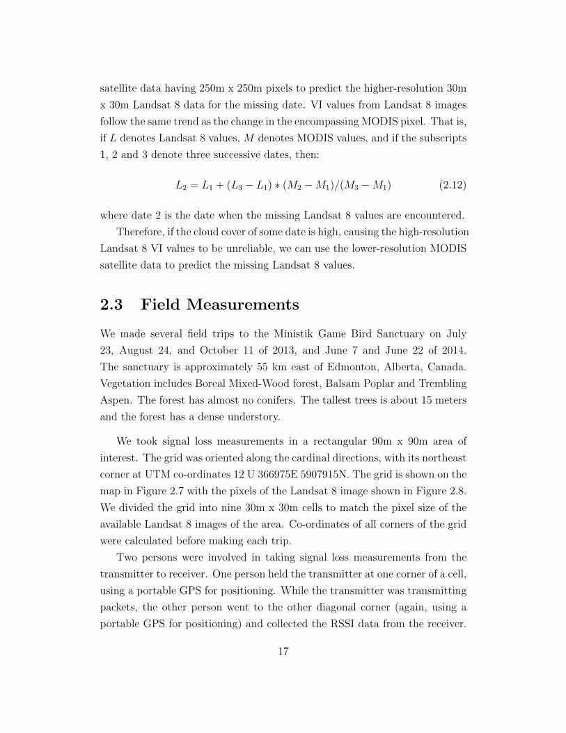
satellite data having 250m x 250m pixels to predict the higher-resolution 30m

x 30m Landsat 8 data for the missing date. VI values from Landsat 8 images

follow the same trend as the change in the encompassing MODIS pixel. That is,

if L denotes Landsat 8 values, M denotes MODIS values, and if the subscripts

1, 2 and 3 denote three successive dates, then:

L2 = L1 + (L3 − L1) ∗ (M2 −M1)/(M3 −M1) (2.12)

where date 2 is the date when the missing Landsat 8 values are encountered.

Therefore, if the cloud cover of some date is high, causing the high-resolution

Landsat 8 VI values to be unreliable, we can use the lower-resolution MODIS

satellite data to predict the missing Landsat 8 values.

2.3 Field Measurements

We made several field trips to the Ministik Game Bird Sanctuary on July

23, August 24, and October 11 of 2013, and June 7 and June 22 of 2014.

The sanctuary is approximately 55 km east of Edmonton, Alberta, Canada.

Vegetation includes Boreal Mixed-Wood forest, Balsam Poplar and Trembling

Aspen. The forest has almost no conifers. The tallest trees is about 15 meters

and the forest has a dense understory.

We took signal loss measurements in a rectangular 90m x 90m area of

interest. The grid was oriented along the cardinal directions, with its northeast

corner at UTM co-ordinates 12 U 366975E 5907915N. The grid is shown on the

map in Figure 2.7 with the pixels of the Landsat 8 image shown in Figure 2.8.

We divided the grid into nine 30m x 30m cells to match the pixel size of the

available Landsat 8 images of the area. Co-ordinates of all corners of the grid

were calculated before making each trip.

Two persons were involved in taking signal loss measurements from the

transmitter to receiver. One person held the transmitter at one corner of a cell,

using a portable GPS for positioning. While the transmitter was transmitting

packets, the other person went to the other diagonal corner (again, using a

portable GPS for positioning) and collected the RSSI data from the receiver.

17

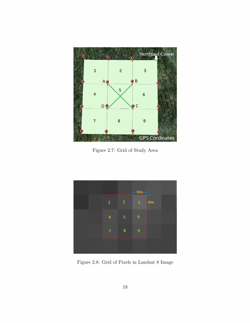
Figure 2.7: Grid of Study Area

Figure 2.8: Grid of Pixels in Landsat 8 Image

18

Walkie-talkies were used to co-ordinate movements from place to place, and

to co-ordinate data gathering. Both the transmitter and receiver were held

approximately one meter above the ground while gathering data. For each

cell, we made the RSSI measurements for two diagonals. Ten RSSI values

were collected for each diagonal. Figure 2.7 demonstrates two diagonal paths

(AC and BD) we were measuring in cell 5. The collected RSSI values from the

two diagonals were averaged for the final result.

2.4 Data Reduction

This section presents the data we collected and how we analyzed them.

2.4.1 Measuring RSSI

We made five separate field trips from June to October in 2013 and 2014, to

collect data in different vegetation densities. Table 2.2 shows the raw data

that we collected in 2013 and 2014.

PPPPPPPPPCellDate

Jul 2013 Aug 2013 Oct 2013 Jun 7, 2014 Jun 22, 2014

1 -94 -98 -89.4 -77.3 -73.02 -101 -98 -89.0 -81.4 -77.43 -100 -94 -88.4 -84.1 -77.64 -97 -95 -87.9 -71.6 -65.15 -98 -89 -96.3 -83.4 -79.76 -101 -96 -93.6 -84.0 -85.27 -94 -95 -91.8 -73.1 -67.98 -95 -90.4 -96.5 -84.1 -78.39 n/a -98 -93.0 -83.9 -78.9

Table 2.2: RSSI (dB) of June to October in 2013 and 2014

These RSSI data are used to calculate α for each cell according to Eq. 2.11. α

values for each cell of different dates are shown in Table 2.6 and 2.7.

19

2.4.2 Interpolating Missing VI Measurements

For August and October of 2013, the cloud cover indices of Landsat 8 images

were 2.36 and 3.45, respectively. These images were clear and they generated

high quality data. However, for July 2013, the cloudiness index was 13.15.

This is extremely high, making the VI calculations for that date unreliable.

To solve the problem of missing Landsat 8 data, we tested the use of lower

resolution MODIS satellite data having 250m x 250m pixels to interpolate

the July Landsat data from the May and September of 2013 Landsat data,

following the same trend as the change in the encompassing MODIS pixel.

May July August September0.57 0.86 0.81 0.75

Table 2.3: NDVI values of MODIS data from May to September of 2013

cell May September Predicted Actual1 0.5772 0.7145 0.7587 0.74392 0.573 0.7177 0.7643 0.74543 0.5784 0.7278 0.7759 0.75384 0.5938 0.7285 0.7719 0.75715 0.5573 0.7239 0.7776 0.75176 0.5153 0.7203 0.7864 0.74987 0.6143 0.7317 0.7695 0.76238 0.5624 0.7326 0.7874 0.76939 0.5676 0.7353 0.7893 0.7631

Table 2.4: Actual and Predicted NDVI Values for August 24, 2013

By applying the model of Eq. 2.12, we first tested this method by comparing

the values it predicts for a date when the Landsat 8 data are available. We

used MODIS and Landsat data from May 20, August 24, and September 9,

2013 (Table 2.3). The actual and predicted values are shown in Table 2.4.

The agreement between the actual and predicted values for August 24 is very

good with the maximum error 4.9%, so we applied this method to calculate

the missing NDVI values for our July 23, 2013 field trip (Table 2.5).

20

cell May July September1 0.5772 0.7984 0.71452 0.5730 0.8061 0.71773 0.5784 0.8191 0.72784 0.5938 0.8108 0.72855 0.5573 0.8257 0.72396 0.5153 0.8456 0.72037 0.6143 0.8034 0.73178 0.5624 0.8366 0.73269 0.5676 0.8378 0.7353

Table 2.5: Predicted NDVI Values for July 23, 2013

2.5 Correlating α to VIs

In this section, we aim to build the correlation model across single cells between

α and VIs. α values are calculated through Eq. 2.11 from raw RSSI data of field

measurements (Table 2.2). VI values are calculated from Landsat 8 satellite

data. First, we correlate models between α and VIs of for each field trip. Then

we build a composite correlation model of all the NDVI and RSSI values from

all of our field trips.

2.5.1 Correlating α to VIs for Each Trip

The raw RSSI data for all field trips is shown in Table 2.6 and 2.7, along with

the values for α calculated from Eq. 2.11, and the Landsat NDVI of each cell.

During our first field trip in July 2013, laptop power constraints prevented us

from collecting RSSI data for the ninth cell. The NDVI values shown for July

2013 are the interpolated values from Table 2.5.

For each field trip, we test linear, logarithmic, and quadratic equations of α

as a function of NDVI. We use two figures of merit, R2 and p, to assess how well

each correlation fits a particular data set. The coefficient of determination,

R2, indicates how well a set of data points fit a regression equation. If the

value of R2 is close one, then the regression equation has a good fit of the

data. The statistical significance of the correlation is (1 − p) so that smaller

values for p are better. p value of 0.05 or less are considered very good. The

21

R2 and p values for all the NDVI models we tested are shown at the end of

the section in Table 2.9.

July 23 August 24 October 11Cell RSSI α NDVI RSSI α NDVI RSSI α NDVI

1 -94 3.256 0.7984 -98 3.502 0.7590 -89.4 3.010 0.43092 -101 3.686 0.8061 -98 3.502 0.7534 -89.0 2.949 0.38623 -100 3.625 0.8191 -94 3.256 0.7491 -88.4 2.888 0.38624 -97 3.440 0.8108 -95 3.318 0.7634 -87.9 2.888 0.45295 -98 3.502 0.8257 -89 2.945 0.7384 -96.3 3.380 0.35156 -101 3.686 0.8456 -96 3.379 0.7466 -93.6 3.195 0.36117 -94 3.256 0.8034 -95 3.318 0.7501 -91.8 3.133 0.42318 -95 3.318 0.8366 -90.4 3.035 0.7424 -96.5 3.379 0.37299 n/a n/a 0.8378 -98 3.502 0.7511 -93.0 3.195 0.3568

Table 2.6: Cell Data of 2013

June 7 June 22Cell RSSI α NDVI RSSI α NDVI

1 -77.3 2.230 0.7126 -78 2.273 0.78952 -81.4 2.482 0.7293 -82 2.529 0.79913 -84.1 2.647 0.7462 -82 2.519 0.79734 -71.6 1.880 0.6730 -65.1 1.479 0.78255 -83.4 2.605 0.7327 -79.7 2.378 0.79776 -84.0 2.642 0.7607 -88 2.888 0.80527 -73.1 1.972 0.6624 -74 2.02 0.7848 -84.1 2.648 0.7582 -84 2.642 0.79889 -83.9 2.630 0.7538 -80 2.396 0.7919

Table 2.7: Cell Data of 2014

Fig. 2.9 to 2.11 show the linear, logarithmic, and quadratic equations for

their fit of α as functions of VIs to the data of July 23, 2013. We can see all

R2 values of the equations are larger than 0.8 and p values less than 0.013,

indicating that these equations fit the data points very well. The equations

predict that α values increase as NDVI values increase, i.e., areas with higher

vegetation density cause more path loss than areas with lower vegetation den-

sity. The linear model is the simplest one and fits the data very well. It

22

reflects how vegetation affects RF propagation in forests by giving a simple

linear mathematical formula of the relationship between α and NDVI. The

more complex quadratic model fits these data extremely well with R2 value

greater than 0.88 and p value less than 0.006. The logarithmic model also fit

the data very well, with R2 and p value a little better than the linear one.

Figure 2.9: Linear Fit of α vs. NDVI on July 23, 2013

Figure 2.10: Logarithmic Fit of α vs. NDVI on July 23, 2013

23

Figure 2.11: Quadratic Fit of α vs. NDVI on July 23, 2013

Fig. 2.12 to 2.14 show the linear, logarithmic, and quadratic equations for

their fit to the data of August 24, 2013. These equations reveal the same

trend between α and VIs as the trip of July 23, 2013, predicting that α values

increase as NDVI values increase. The equations also fit the data very well

with good R2 and p values. The complex quadratic model has the highest

R2 value and lowest p value. The logarithmic model also has good R2 and p

values, but it is not significantly better than the simpler linear model.

Figure 2.12: Linear Fit of α vs. NDVI on August 24, 2013

24

Figure 2.13: Logarithmic Fit of α vs. NDVI on August 24, 2013

Figure 2.14: Quadratic Fit of α vs. NDVI on August 24, 2013

25

Fig. 2.15 and 2.16 are linear equations of α as functions of NDVI from data

sets of June 7 and June 22, 2014, respectively.

Figure 2.15: Linear Fit of α vs. NDVI on June 7, 2014

Figure 2.16: Linear Fit of α vs. NDVI on June 22, 2014

26

These two linear equations (Fig 2.15 and 2.16) show that α value increase

as NDVI values increase, which reveals the same trend between α and VIs

as the trips of July 23 and August 24 in 2013. For the trip of June 7, 2014,

the linear model as well as the logarithmic and quadratic models fits the data

points extremely well with R2 value greater than 0.93 and p value less than

0.00002. The equations of June 22, 2014 also have very good R2 and p values

(R2 > 0.8473 and p < 0.0004). R2 and p values of logarithmic and quadratic

correlation models of the two dates are shown in Table 2.9.

Figure 2.17 is the linear fit of α as a function of NDVI from data set on Oc-

tober 11, 2013. The correlation is qualitatively different than the other dates,

giving an inverse relationship between α and NDVI. The linear model (plus

its logarithmic and quadratic models) predicts that α values should decrease

as NDVI values increase. The correlation also exhibits a much lower value

of R2 and a much higher value of p than the other dates, indicating that the

correlation model of October is unreliable.

Figure 2.17: Linear Fit of α vs. NDVI in October, 2013

27

2.5.2 The Composite Correlation Model

So far, we have characterized the correlation models between α and VI values

for each field trip. However, each model only reflects the relationship between

α and VIs in a “local” range of VI values. For example, NDVI values may

vary from 0.65 to 0.7 of the correlation model in June, from 0.8 to 0.85 in July,

and from 0.74 to 0.76 in August. Thus, there are some gaps of the range of

NDVI values that may not be covered by any of the correlation models.

To characterize the relationship between α and NDVI through a wider

range of VI values in a more consistent way, e.g., from 0.65 to 0.85, we correlate

a composite model of all the RSSI data and NDVI values from all of our field

trips of the leaf-on conditions. Data of October 2013 are not selected because

the correlation model of October is unreliable. Fig 2.18 shows data points of

all NDVI and α values of all of our field trips except October 2013.

Figure 2.18: NDVI and α Values from All Field Trips

Excluding Outliers

As Fig. 2.18 consists of all NDVI and α values of all of our filed trips of different

dates, it may include some outliers that behave differently than the other data

points. For example, the circled data point (0.7825, 1,4745) in Fig 2.19 is

28

from cell 4 of date June 22, 2014. It has NDVI value of 0.7825 and α value

of 1.4745. However, other data points with NDVI value of about 0.78 usually

have α values greater than 2.5. The point also has the lowest α value that is

very distant from all the other points. Therefore, this point may be an outlier.

Figure 2.19: An Outlier of All the Data Points

To detect outliers from all the data points, we test the linear equation for its

fit of α to NDVI for each individual cell consisting of RSSI and NDVI values of

the four different dates. The equation of each cell should follow the trend that

α increases as NDVI increase and exhibit strong correlation. If the equation

fits the data of a cell very well with a good R2 value, all the data points in

the cell can contribute to the composite correlation model. Otherwise, the

equation has a poor fit to the data and there may be some outliers in the cell.

Then we should test the quality of the fit of α to NDVI after deleting the

suspected point of the cell. If there is a much better fit of α to NDVI after

removing the suspected point, the point is considered as an outlier and does

not contribute to the composite correlation model.

Fig. 2.20 to 2.23 show the linear fits of α as functions of NDVI to the data

in cell 2, 5, 7, and 8. Each figure consists of NDVI and RSSI values from

the four different dates of one cell. Each equation fits the data very well with

good R2 values. The R2 values of cell 2, 5, 7, and 8 are 0.7474, 0.862, 0.8737,

and 0.9551, respectively. Therefore, NDVI and α values in these cells can

contribute to the composite correlation model.

29

Figure 2.20: Linear Fit of α to VIs for Cell 2 Consisting of NDVI and α Valuesfrom Different Dates


30



31

Cell 2, 5, 7, and 8 have very good fit of α to NDVI for each one. However,

other cells do not have as good fit of α to NDVI as these four cells. Fig. 2.24

shows the α and NDVI values of cell 4 of the four dates. The linear equation

has a poor fit of α to NDVI with a very low R2 value. The circled point (0.7825,

1.4745) from June 22, 2014, same as in Fig. 2.19, behaves very differently than

the other data points in the cell. If we delete the circled point, a linear equation

shows a much better fit to the data with R2 value of 0.9265 (see Fig. 2.25).

Thus, the circled point is considered as an outlier.

Figure 2.24: Linear Fit of α to VIs for Cell 4

Figure 2.25: Linear Fit of α to VIs for Cell 4 after Removing the Outlier

32

For cell 1, 3, and 6, we also detect one outlier out of each cell. Fig. 2.26

shows that in cell 1, the data point (0.759, 3.5) from August 2013 deviates

from the other points. After deleting this point, we have a better linear fit

with R2 of 0.7325. Fig. 2.27 detects another suspected point at (0.7491, 3.13)

from August 2013 in cell 3. The equation shows a much better linear fit with

R2 of 0.8647 to the data without the point. Cell 6 also detects an abnormal

point at (0.7466, 3.379) from August 2013. Fig. 2.28 shows a very good fit of

α to NDVI with R2 of 0.9802 after removing the abnormal point. Therefore,

these abnormal points in each cell are considered as outliers.



33


For the ninth cell, we have only three data points in total as laptop power

constraints prevented us from collecting RSSI data for the cell in July 23, 2013.

The number of points is small for us to determine whether the cell contains

any outliers or not. We consider adding data points of other cells to help

determine the quality of data in the ninth cell. As the eighth cell has a very

good fit of α to NDVI with R2 of 0.9551 (see Fig. 2.23), we combine the data

of cell 8 and 9 and test the qualify of the linear fit to the data. We detect a

point at (0.7511, 3.5) from August 2013 that deviates from the other points.

Fig. 2.29 shows a much better linear equation of α to NDVI with R2 of 0.8892

after deleting the point.

Figure 2.29: Linear Fit of α to VIs for Cell 8 and 9 after Removing the Outlier

34

Fig. 2.25 to 2.29 all show much better linear fits of α to NDVI with good

R2 values after deleting the abnormal points in each cell. These points are

considered as outliers. One similarity of the outliers in cell 1, 3, 6, and 9 is

that they all come from the data of August 2013. It implies that data points in

August 2013 behave differently than the other dates. The correlation model of

August 2013 is not as reliable as correlation models of the other dates on July

23, 2013, June 7, 2014, and June 22, 2014. The reason for this abnormality in

August 2013 may be caused by the weather conditions such as wind. We know

that wind can interfere with signal transmission and affect the received signal

strength. Future considerations of weather conditions should be recorded in

more detail when taking field trip measurements.

Correlating the Composite Model

After excluding the outliers in cell 1, 3, 4, 6, and 9, we can use the other data

points in these cells to build the composite correlation model between α and

VIs. We test the linear, logarithmic, and quadratic equations for their fit to

the data. Fig. 2.30 to 2.32 are these equations for their fits to the data points.

Figure 2.30: Linear Fit of α vs. NDVI of the Composite Correlation

35

Figure 2.31: Logarithmic Fit of α vs. NDVI of the Composite Correlation

Figure 2.32: Quadratic Fit of α vs. NDVI of the Composite Correlation

36

The equations of the composite correlation model predict that α values

increase as NDVI increase. All the equations have very good fits of α to NDVI

with R2 greater than 0.77 and extremely small p values that are less than

7.4E − 10, indicating these correlations have high statistical significance. The

quadratic and logarithmic equations are only a little better than the simpler

linear model. The composite correlation also exhibit a wide range of NDVI

values, varying from 0.65 to 0.85, which covers the whole in-leaf season in

forests.

Test for Normality

We use the normal probability plot to test the distribution of the data. The

RSSI values in this composite model should exhibit relatively normal distribu-

tion. First, we order RSSI values from 1 to N. Then, we use the formula i−0.5N

(i = 1, 2, ..., N) to find z-values from the normal distribution table. Table 2.8

shows the RSSI and z-values. Fig 2.33 is the ordered RSSI values plotted

against the z-values. The plot shows that the RSSI values are falling close to

a straight line. Therefore, the RSSI data are fairly normal distributed.

i RSSI (i− 0.5)/N z-value i RSSI (i− 0.5)/N z-value1 -101 0.019 -2.09 15 -89 0.537 0.092 -100 0.056 -1.59 16 -87 0.574 0.193 -98 0.092 -1.32 17 -87 0.611 0.284 -97 0.129 -1.13 18 -86 0.648 0.385 -95 0.167 -0.97 19 -84 0.685 0.486 -95 0.203 -0.84 20 -84 0.722 0.597 -94 0.241 -0.7 21 -84 0.759 0.78 -94 0.278 -0.59 22 -84 0.796 0.839 -92 0.315 -0.48 23 -83 0.833 0.9710 -92 0.352 -0.38 24 -81 0.870 1.1311 -91 0.389 -0.28 25 -77 0.907 1.3212 -90 0.426 -0.19 26 -73 0.944 1.5913 -90 0.463 -0.09 27 -72 0.981 2.0914 -90 0.5 0

Table 2.8: RSSI and z-values

37

Figure 2.33: Normal Probability Plot

Test for Randomness

We test the randomness of our data by using the residuals from the linear

composite model. For a given number N of discrete observations,the Fourier

series to the residuals are:

n(m) = a0 +N∑m=1

(ai ∗ cos(2πmf(i)) + bi ∗ sin(2πmf(i))) (2.13)

where

ai = (2/N)∑N

m=1 n(m)cos(2πmf(i))

bi = (2/N)∑N

m=1 n(m)sin(2πmf(i))

f(i) = i/N , i = 1, 2, ..., q

m = 1, 2, ..., N

N = 2q + 1, if N is an odd number

N = 2q is N is an even number.

The intensity values in the frequency domain is defined as:

I(f(i)) = (N/2)(a2i + b2i ) (2.14)

38

Then, we plot the cumulative periodogram by adding up the intensity

values:

C(f(i)) =

∑ij=1 I(f(j))∑qj=1 I(f(j))

i = 1, 2, ..., q (2.15)

Figure 2.34: Cumulative Periodogram

If the residual series exhibit a distribution of Gaussian white noise, then

the variables generated by C(f(i)) will follow a straight line close to yi =

2∗f(i) from (0,0) to (0.5,1). The cumulative intensity values in Fig. 2.34 shows

closeness to the straight line, indicating that our data follows the Gaussian

white noise and are randomly distributed.

2.6 Results and Discussion

We tested linear, logarithmic, and quadratic equations for their fit to the data

of each field trip as well as data of all NDVI and RSSI values from all of our

trips. The R2 and p value for each correlation model is shown in Table 2.9.

For the data from July 23 and August 24 of 2013, and June 7 and June 22

of 2014, we found that the simplest model, the linear function, fits NDVI to α

very well. These models have R2 values greater than 0.80 and p values of 0.014

39

Linear Logarithmic QuadraticR2 p R2 p R2 p

July 2013: α-NDVI 0.8160 0.0136 0.8201 0.0130 0.8812 0.0056August 2013: α-NDVI 0.8044 0.0025 0.8065 0.0025 0.8677 0.0012October 2013: α-NDVI 0.4233 0.0577 0.4334 0.0538 0.4766 0.0396June 7, 2014: α-NDVI 0.9338 0.00002 0.9348 0.00002 0.9357 0.00002June 22, 2014: α-NDVI 0.8473 0.0004 0.8485 0.0004 0.8672 0.0003

Composite α-NDVI 0.7732 7.33E-10 0.7755 6.4E-10 0.7755 6.43E-10

Table 2.9: Suitability of Regression Models

or better. The slightly more complex quadratic model fits these data extremely

well. The logarithmic model for these data also has very good values of R2

and p, but they are not significantly better than the simpler linear model.

However, the correlation for the data of October 2013 is qualitatively differ-

ent than the other dates, giving an inverse relationship between α and NDVI.

It predicts that α should decrease as NDVI increases. This correlation also

exhibits a much lower value of R2 and a much higher value of p than the other

correlations. The explanation for this dramatic shift is an equally dramatic

change in the forest: during June to August, the trees were in-leaf. By the

time we visited the site in October, the trees had dropped their leaves, and

the forest was out-of-leaf. This can be observed in the change in NDVI values.

From June to August, NDVI ranges from 0.65 to 0.85. The high NDVI values

correspond to densely vegetated areas that can largely affect RF propagation.

However, in October, the NDVI values are much lower, and range from 0.35 to

0.46, which indicates the area is out-of-leaf and RF propagation is no longer

affected by vegetation. The satellite sensor, of course, was still receiving re-

flectance data from the area of interest in October, likely from fallen leaves

decomposing on the forest floor [25].

We conclude that our proposed method of using NDVI data to predict α is

only applicable when the forest is in-leaf. Further work is required to predict

path loss in the out-of-leaf condition. As noted earlier, the underlying model

would also have to change, as multi-path propagation becomes important in

this condition.

40

We also build a composite correlation model of all RSSI and NDVI values

from all of our field trips except October. By analyzing the qualify of data

in each individual cell consisting of α and NDVI values of different dates, we

found that cell 2, 5, 7, and 8 have very good fit of α to NDVI. The other

cells, however, have abnormal points that deviate from the other data points.

We tested the improvement of the linear fit after deleting the abnormal points

for each cell. Each cell exhibits a much better linear fit without the outliers.

After excluding the outliers, we use all the other data points to characterize the

relationship between α and NDVI. We tested linear, logarithmic, and quadratic

equations for their fit to the data points. The equations fit the data very well

with R2 larger than 0.77 and extremely small p value less than 7.4E − 10.

The logarithmic and quadratic models are only a little better than the simpler

linear model.

The composite correlation model consists of much more data points than

the correlation model of single dates. The model detects outliers by analyzing

the quality of data in single cells. It finds that most of the outliers come from

the data of August 2013, which implies that the correlation model in August is

not as reliable as the other dates. Moreover, the composite correlation model

covers a wider range of NDVI values, varying from 0.65 to 0.85, and reflects

how vegetation affects the RF propagation in a more consistent way than the

correlations of single dates. The composite correlation is representative of the

relationship between α and VIs from field measurement in June, July, and

August. As NDVI values in September vary from 0.65 to 0.75, which are also

in the range of the composite correlation model, we can apply the model to

the time from June to September, i.e., the whole in-leaf season in forests.

To summarize, we characterize the relationship between α and NDVI of

different dates. We found that a quadratic model has the best ability to

predict α from satellite NDVI measurements. However, a simpler linear model

also performs quite well. We also correlate a composite model of all NDVI

and RSSI values from all of our field trips. The composite correlation model

covers a wide range of NDVI values and can be applied to the whole in-leaf

phrase in forests.

41

Chapter 3

Predicting Path Loss across

Multiple Cells

After we build the correlation model across single cells between path loss

exponent, α, and vegetation indices (VIs), we can use the model to predict

path loss across multiple cells. First, with available satellite data, we can get

VI values of all cells in the area of interest. By applying the VI values to the

correlation model, we can get α values for each cell. Then, we use a heuristic

weighted sum method to calculate the overall α value for a path crossing

multiple cells, and to predict the RSSI value based on the path’s distances

in each crossing cell. Finally, we compare the predicted RSSI values against

actual field data retrieved from SensorCloud that gathers RSSI from deployed

sensors to an aggregator in the area of interest.

3.1 Weighted Sum Model

For a path crossing multiple cells where each cell has a different vegetation

density, and thus a different value of α, we need to determine the overall α

value of this path to calculate the received signal strength. Figure 3.1 shows

a path AC that crosses two cells—cell 5 with distance AB = d1 and cell 8

with distance BC = d2. The previous path loss model for areas with varying

42

vegetation densities is:

log Pr(d) = −α ∗ log d+ log K + log Pt (3.1)

where d = d1 + d2, and Pt and K are constants once the radios and antennas

have been selected. The only factor left unknown to calculate the received

power Pr(d) is the α value for path AC that crosses two cells with different α

values in each cell.

Figure 3.1: A Path across Multiple Cells

In this work, we propose a weighted sum method to determine the overall

α value for one path across multiple cells. With available satellite data, we can

get VI values of each cell in the area of interest. By applying the VI values to

the correlation model concluded in chapter 3, we can get α value for each cell.

To get the overall α value for the path, we consider distances in each crossing

cell. The following gives the definition of the weighted sum method:

For a path that crosses multiple cells c1, c2, ..., cn with distances d1, d2, ..., dn

43

and path loss exponent α1, α2, ..., αn in each cell, we define the path’s overall

path loss exponent α′ as:

α′ =d1 × α1 + d2 × α2 + ...+ dn × αn

d1 + d2 + ...+ dn(3.2)

α′ =

∑dm × αm∑

dim, i = 1, 2, ..., n. (3.3)

In Figure 3.1, assuming α1 in cell 5 is 2.0, α2 in cell 8 is 3.0, d1 = 20m,

and d2 = 15m, the overall path loss exponent α′ for path AC is:

α′ =α1 ∗ d1 + α2 ∗ d2

d1 + d2=

2.0 ∗ 20 + 3.0 ∗ 15

20 + 15= 2.43 (3.4)

3.2 SensorCloud Data

The weighted sum method allows us to calculate the overall path loss exponent

between any two locations whose path crosses multiple cells. To test our

correlation model, we need to compare the predicted RSSI against real field

data. To obtain real field data, we deploy wireless sensor nodes in a testing

area and use an aggregator to gather RSSI data from each sensor. The RSSI

data is displayed online on SensorCloud.

Lord MicroStrain’s SensorCloud provides a method of gathering data re-

motely from sensor networks, which enables people to collect RSSI data with-

out the need to go to field. An MicroStrain WSDA-1000-LXRS Aggregator is

used (see Fig. 3.2) to connect field wireless sensor nodes to SensorCloud [26].

After installing the aggregator and building the connection between wireless

nodes and SensorCloud, the aggregator can detect and display the RSSI val-

ues online in SensorCloud. Thus, we can view and download RSSI data from

each sensor to the aggregator online. Figure 3.4 is a visualization plot that

shows the RSSI data for the paths from each field sensor to the aggregator on

September 25, 2013.

44

Figure 3.2: The WSDA Aggregator Deployed in the Field

45

3.3 Multi-cell Path Loss Calculations

In this section, we describe our network site that consists of eight sensors and

one aggregator for multi-cell path loss calculations. We calculate the overall

α value and RSSI data for paths from each sensor to the aggregator based on

the weighted sum method. The predicted RSSI values are compared against

real field data gathered from the aggregator and displayed on SensorCloud.

3.3.1 Calculating Path Loss Using the Correlation Model

We select the same grid as our work site as for determining the correla-

tion model between α and vegetation indices. Eight wireless sensor nodes

(No. 223—230) and one aggregator are deployed through the nine cells (see

Figur 3.3).

Figure 3.3: Deployment of Aggregator and Sensor Nodes

We select September 25, 2013 and June 8, 2014 as the testing dates when

Landsat 8 data are available. As our correlation model is only applicable to in-

leaf forests, the time between October 2013 and May 2014 when trees are out-

of-leaf is not selected as our testing date for multi-cell path loss calculations.

As the sensors used here are different from what we used in the previous

46

correlation model, the value of K and Pt are also different. However, the values

of K and Pt are fixed once the radios and antennas have been selected; thus,

like in section 3.1, we select a cell with constant α value and use SensorCloud’s

RSSI data from sensors in the cell to determine K and Pt. We choose the

middle cell that contains the aggregator, sensor 224, and sensor 228. We

retrieve the RSSI data from the two sensors on September 25, 2013. The

average RSSI received at the aggregator is -56 dB from sensor 224 with distance

20.4m and -41 dB from sensor 228 with distance 3m. From equation 3.1, we

have:

−4.1 = log K + log Pt − α ∗ log 3 (3.5)

−5.6 = log K + log Pt − α ∗ log 20.4 (3.6)

We find the value of log K + log Pt is -3.4, and α value of cell 5 is 1.67.

We choose the linear composite correlation model concluded from all the

leaf-on measurements in chapter 3 (see Fig 2.30). The correlation has R2 of

0.7732 and extremely small p value that exhibits high statistical significance:

α = 8.7796 ∗NDV I − 3.8393 (3.7)

We first calculate NDVI values of the nine cells in the grid. Then by

applying the correlation model of Eq. 3.7, we get the α values for each cell.

Table 3.1 shows NDVI and α values for the two testing dates. The predicted

α value of September 25, 2013 of cell 5 is 1.69, which is very close to the α

value of 1.67 calculated from actual RSSI data in Eq. 3.5 and 4.6. It indicates

that the correlation model in Eq. 3.7 reveals a good relationship between α

and vegetation density in forests.

After we get the α values of the nine cells in the grid, we can apply the

weighted sum method to calculate the overall α value from each sensor to the

aggregator. Since co-ordinates of the aggregator and sensors are known, we

can calculate the total distance from each sensor to the aggregator as well as

distances in each path’s crossing cells. Table 3.2 shows the crossing cells from

each sensor to the aggregator. Each line indicates the cell numbers that a path

47

Sep 25, 2013 June 8, 2014Cell NDVI α NDVI α

1 0.6138 1.5496 0.7491 2.73752 0.6219 1.6207 0.7408 2.66023 0.6620 1.9728 0.7562 2.79984 0.6392 1.7726 0.7583 2.81825 0.6297 1.6892 0.7474 2.72266 0.6364 1.7480 0.7266 2.54007 0.6337 1.7243 0.765 2.87718 0.6383 1.7647 0.7632 2.86139 0.6475 1.8455 0.7599 2.8323

Table 3.1: NDVI and α Values for Each Cell of the Testing Dates

is crossing, and the distance traversed in each cell. For example, the path from

sensor 223 to the aggregator crosses 25 meters of cell 2 and 18 meters of cell

5.

sensor n crossing distances into the aggregator cells each crossing cell (m)

223 2, 5 25, 18224 5 20.4225 8, 5 12.5, 12.5226 7, 8, 5 15.8, 2.5, 29.2227 4, 5 15, 27228 5 3229 1, 2, 5 15, 32.3, 4.4230 5 26.2

Table 3.2: Distances of Paths Across Each Cell

Based on the distances in the cells crossed by each path, and α values from

Table 3.1 and 3.2, we apply the weighted sum method of Eq. 3.2 to get the

overall α value for each sensor to the aggregator. The overall α values and

predicted RSSI data for each path are shown in Table 3.3 and 3.4.

48

3.3.2 Comparison between Predicted and Actual RSSI

Real field RSSI data are extracted from SensorCloud of Sep 25, 2013 and

June 8, 2014 when Landsat 8 are available on these dates. Figure 3.4 is a

visualization plot of RSSI data from different sensors on September 25, 2013.

For each testing date, we record the RSSI values from SensorCloud every ten

minutes and for 24 hours. We use the average values for the final result (see

Table 3.3 and 3.4).

Figure 3.4: Actual RSSI Data Displayed on SensorCloud from Different Sen-sors to the Aggregator

Table 3.3 and 3.4 list the overall α values, the predicted RSSI, and the

actual field RSSI values from each sensor to the aggregator. Because some

sensors have been damaged by June 2014 (e.g., 225 and 229), the actual RSSI

values from those sensors are missing.

3.4 Results and Discussion

We use the mean absolute percentage error (MAPE) to measure the accuracy

of the RSSI prediction from our correlation model. MAPE measures how close

49

predictions are to the eventual outcomes. The definition is:

M =100%

n

n∑t=1

|At − FtAt

| (3.8)

where At is the actual value and Ft is the forecast value. In our case, At is

the actual RSSI from SensorCloud and Ft is the predicted RSSI. For the data

tested on September 25, 2013, we have M = 3.68%. For the data from June

8, 2014, M equals 4.78%. The predicted RSSI is very close to the actual RSSI

from Table 3.3 and 3.4.

Sensor n overall α value predicted RSSI actual RSSI223 1.6494 -60.94 -61.8224 1.6892 -56.12 -55.71225 1.727 -58.14 -56.33226 1.7049 -62.59 -64.0227 1.7190 -61.9 -64.2228 1.6892 -42.06 -40.92229 1.6059 -61.52 -55.0230 1.6892 -57.95 -54.0

Table 3.3: Predicted and Actual RSSI Data from Each Sensor to the Aggre-gator of September 25, 2013

Sensor n overall α value predicted RSSI actual RSSI223 2.6863 -77.88 -76224 2.7226 -69.66 -62.0225 2.792 -73 n/a226 2.7813 -80.64 -79227 2.7568 -78.75 -77.2228 2.7226 -46.99 -43229 2.6772 -79.87 n/a230 2.7226 -72.62 -73

Table 3.4: Predicted and Actual RSSI Data from Each Sensor to the Aggre-gator of June 8, 2014

50

We conclude that our correlation model from single cells predicts path loss

across multiple cells very well with an error less than 5%. With satellite data

available anywhere on earth, the model enables us to get the α value for each

30m x 30m cell that corresponds to a Landsat 8 pixel. With the weighted sum

method, we can calculate the path loss between any two locations whose path

crosses multiple cells.

51

Chapter 4

Conclusions and Future Work

We propose a relatively simple correlation model of different dates to predict

values for the path loss exponent, α, based on satellite observations of VIs.

We also characterize the composite correlation of α to VIs of all the filed mea-

surements, which covers the whole in-leaf phrase in forests. We found this

approach to work very well for leaf-on conditions in a study site consisting of

boreal forest in central Alberta, which is specific to aspen boreal forests that

cover approximately 1.5 to 2.0 million square kilometers in Canada alone.

The correlations are strong (R2 > 0.77) and exhibit high statistical signif-

icance (p < 0.01). The correlations enables us to characterize and predict

the RF propagation environment in forested areas without the need for field

measurements, given that satellite data are available any location on Earth.

We also propose a method to fill in missing high-resolution 30m x 30m data

for dates where the satellite’s view of the area of interest is obscured by clouds

or aerosols such as pollution or sand storms degrade or significantly interfere

with the high-resolution satellite data we are using. We tested our proposal

by comparing its predictions to actual values for a date when the 30m x 30m

data are available, and the results show absolute errors of less than 5%.

Finally, we apply the correlation model between α and VIs to predict path

loss across multiple cells. With available Landsat 8 data, the correlation model

enables us to get the α value for each cell in the area of interest. By using

the weighed sum method, we can calculate the overall α and RSSI for a path

between any two locations. The predicted RSSI are compared with actual field

52

data retrieved from SensorCloud that that gather RSSI from each sensor to the

aggregator deployed in the area of interest. Results show that the predicted

RSSI values are very close to the real ones with error less than 5%.

Based on these promising initial results, future research includes taking

more field RSSI measurements in forested areas. Carrying out field measure-

ments in each month when trees are in-leaf will enable us to develop much

more extensive correlations between α and vegetation densities for the entire

leaf-on phase in boreal forest sites. Also, details about the weather conditions

such as the wind speed should also be recorded and considered carefully to

make the measured RSSI data more reliable when taking field trips. These

correlations will provide much more complete information for people who want

to design and deploy WSNs in fields.

53

Bibliography

[1] K. Y. Kaneshiro, M. H. Kido, C. W. Mundt, K. N. Montgomery, A. Asquith,and D. W. Goodale, “Integration of wireless sensor networks into cyberinfras-tructure for monitoring Hawaiian “mountain-to-sea” environments.” Environ-mental Management, vol. 42, no. 4, pp. 658–666, 2008.

[2] X. Han, X. Cao, E. Lloyd, and C.-C. Shen, “Fault-tolerant relay node place-ment in heterogeneous wireless sensor networks,” IEEE Transactions on MobileComputing, vol. 9, no. 5, pp. 643–656, May 2010.

[3] E. Oyman and C. Ersoy, “Multiple sink network design problem in large scalewireless sensor networks,” 2004 IEEE Int’l Conf. on Communications, pp.3663–3667 Vol.6, 2004.

[4] Y. Turkogullari, N. Aras, I. Altinel, and C. Ersoy, “An efficient heuristic forplacement, scheduling and routing in wireless sensor networks,” Ad Hoc Net-works, vol. 8, pp. 654–667, 2010.

[5] S. Burgess, M. Kranz, N. Turner, R. Cardell-Oliver, and T. Dawson, “Har-nessing wireless sensor technologies to advance forest ecology and agriculturalresearch,” Agricultural and Forest Meteorology, vol. 150, no. 1, pp. 30–37, Jan.2010.

[6] Y. Meng, Y. Lee, and B. Ng, “Study of propagation loss prediction in forestenvironment,” Progress In Electromagnetics Research B, vol. 17, pp. 117–133,2009.

[7] ITU-R, “ITU-R Recommendation P.833-7 Attenuation in Vegetation,” 2012.

[8] M. H. C. Dias and M. S. de Assis, “An empirical model for propagation lossthrough tropical woodland in urban areas at UHF,” IEEE Trans. on Antennasand Propagation, vol. 59, no. 1, pp. 333–335, Jan. 2011.

[9] N. Rogers, A. Seville, J. Richter, and D. Ndzi, “A generic model of 1-60 GHzradio propagation through vegetation-final report,” no. May, p. 152, 2002.

[10] N. Sabri, S. A. Aljunid, M. S. Salim, R. Kamaruddin, R. Ahmad, and M. Malek,“Path loss analysis of wsn wave propagation in vegetation,” 2013.

54

[11] P. Mestre, C. Serdio, R. Morais, J. Azevedo, and P. Melo-Pinto, “Vegetationgrowth detection using wireless sensor networks,” 2010.

[12] I. Kovacs, P. Eggers, and K. Olesen, “Radio channel characterisation for forestenvironments in the VHF and UHF frequency bands,” in Vehicular TechnologyConference, no. 3, 1999, pp. 1387–1391.

[13] J. Voldhaug, “Deployable WiMAX in a forest area; channel measurements andmodelling,” in 2010 Military Communications Conference, 2010, pp. 737–742.

[14] Y. Meng and Y. Lee, “Investigations of foliage effect on modern wireless com-munication systems: A review,” Progress In Electromagnetics Research, vol.105, pp. 313–332, 2010.

[15] L.-W. Li, T.-S. Yeo, P.-S. Kooi, and M.-S. Leong, “Paths through a four-layeredmodel of rain forest : An analytic approach,” IEEE Trans. on Antennas andPropagation, vol. 46, no. 7, pp. 1098–1111, 1998.

[16] I. Cuinas, J. Gay-Fernandez, P. Gomez, A. V. Alejos, and M. G. Sanchez,“Radioelectric propagation in mature wet forests at 5.8 GHz,” in 2009 IEEEAntennas and Propagation Society International Symposium. IEEE, Jun. 2009,pp. 1–4.

[17] R. D. Jackson and A. R. Huete, “Interpreting vegetation indices,” PreventiveVeterinary Medicine, vol. 11, pp. 185–200, 1991.

[18] “Measuring vegetation,” Website, http://earthobservatory.nasa.gov/Features/MeasuringVegetation/.

[19] SEOS, “Supplement - vegetation spectral signature,” Website, http://www.seos-project.eu/modules/agriculture/agriculture-c01-s01.html.

[20] J. R. Jensen, Remote Sensing of the Environment: An Earth Resource Perspec-tive, 2000.

[21] Y. Gu, B. K. Wylie, D. M. Howard, D. M. Howard, and L. Ji, “Ndvi saturationadjustment: A new approach for improving cropland performance estimates inthe greater platte river basin, usa,” 2013.

[22] X. Xiong, B. N. Wenny, A. Angal, W. Barnes, and V. Salomonson, “Summaryof Terra and Aqua MODIS long-term performance,” in Geoscience and RemoteSensing IEEE International Symposium, 2011, pp. 4006–4009.

[23] USGS, “Usgs landsat mission,” Website, http://landsat.usgs.gov/landsat8.php/.

[24] EROS, “Usgs global visualization viewer,” Website, http://glovis.usgs.gov/.

55

http://earthobservatory.nasa.gov/Features/MeasuringVegetation/

http://earthobservatory.nasa.gov/Features/MeasuringVegetation/

http://www.seos-project.eu/modules/agriculture/agriculture-c01-s01.html

http://www.seos-project.eu/modules/agriculture/agriculture-c01-s01.html

http://landsat.usgs.gov/landsat8.php/

http://landsat.usgs.gov/landsat8.php/

http://glovis.usgs.gov/

[25] K. Huemmrich, T. Black, P. Jarvis, J. McCaughey, and F. Hall, “High tem-poral resolution NDVI phenology from micrometeorological radiation sensors,”Journal of Geophysical Research, vol. 104, no. D22, pp. 27 935–27 944, Nov.1999.

[26] Lord-MicroStrain, “Sensorcloud,” Website, http://www.microstrain.com/wireless/sck/.

56

http://www.microstrain.com/wireless/sck/

http://www.microstrain.com/wireless/sck/

Predicting RF Path Loss in Forests Using Satellite ...

Documents