Predicting Hydrophobic Solvation by Molecular Simulation: 2. New United-atom Model for Alkanes, Alkenes and Alkynes Miguel Jorge* Department of Chemical and Process Engineering, University of Strathclyde, 75 Montrose Street, Glasgow G1 1XJ, United Kingdom Email – [email protected] Abstract: Existing united-atom models for non-polar hydrocarbons lead to systematic deviations in predicted solvation free energies in hydrophobic solvents. In this paper, an improved set of parameters is proposed for alkane molecules that corrects this systematic deviation and accurately predicts solvation free energies in hydrophobic media, while simultaneously providing a very good description of pure liquid densities. The model is then extended to alkenes and alkynes, again yielding very accurate predictions of solvation free energies and densities for these classes of compounds. For alkynes in particular, this work represents the first attempt at a systematic parameterization using the united-atom approach. Averaging over all 95 solute/solvent pairs tested, the mean signed deviation from experimental data is very close to zero, indicating no systematic error in the predictions. The fact that predictions are robust even for relatively large molecules suggests that the new model may be applicable to solvation of non-polar macromolecules without accumulation of errors. The root mean squared deviation of the simulations is only 0.6 kJ/mol, which is lower than the estimated uncertainty in the experimental measurements. This excellent performance constitutes a solid basis upon which a more general model can be parameterized to describe solvation in both polar and non-polar environments. Keywords: Solubility; Molecular Simulation; hydrocarbons; non-polar; free energy

Welcome message from author
This document is posted to help you gain knowledge. Please leave a comment to let me know what you think about it! Share it to your friends and learn new things together.
Transcript

Predicting Hydrophobic Solvation by Molecular
Simulation: 2. New United-atom Model for Alkanes,
Alkenes and Alkynes
Miguel Jorge*
Department of Chemical and Process Engineering, University of Strathclyde, 75 Montrose
Street, Glasgow G1 1XJ, United Kingdom
Email – [email protected]
Abstract: Existing united-atom models for non-polar hydrocarbons lead to systematic
deviations in predicted solvation free energies in hydrophobic solvents. In this paper, an
improved set of parameters is proposed for alkane molecules that corrects this systematic
deviation and accurately predicts solvation free energies in hydrophobic media, while
simultaneously providing a very good description of pure liquid densities. The model is then
extended to alkenes and alkynes, again yielding very accurate predictions of solvation free
energies and densities for these classes of compounds. For alkynes in particular, this work
represents the first attempt at a systematic parameterization using the united-atom approach.
Averaging over all 95 solute/solvent pairs tested, the mean signed deviation from
experimental data is very close to zero, indicating no systematic error in the predictions. The
fact that predictions are robust even for relatively large molecules suggests that the new
model may be applicable to solvation of non-polar macromolecules without accumulation of
errors. The root mean squared deviation of the simulations is only 0.6 kJ/mol, which is lower
than the estimated uncertainty in the experimental measurements. This excellent performance
constitutes a solid basis upon which a more general model can be parameterized to describe
solvation in both polar and non-polar environments.
Keywords: Solubility; Molecular Simulation; hydrocarbons; non-polar; free energy

1 - Introduction
Predicting solvation in hydrophobic environments is relevant for a wide range of
processes, from industrial separations to protein-ligand binding [1-4]. However, it has been
largely overlooked in previous molecular simulation studies, which have primarily focused
on aqueous solvation (or hydration) processes [5-7]. Moreover, most interaction potential
models, or force-fields, suitable for use in solution have been parameterized against bulk
liquid properties. For example, the widely used OPLS model was parameterized to match
pure liquid densities and enthalpies of vaporization [8]. A notable exception to this trend is a
recent version of the GROMOS force-field [9], where experimental solvation free energies
were used as target properties in the parameterization procedure. Interestingly, the authors
developed two alternative version of the model, one optimized for pure liquid properties
(version 53A5) and another for solvation free energy calculations (version 53A6). However,
the parameters for alkanes, the archetypal hydrophobic molecules, were taken directly from a
previous parameter set [10], where pure liquid densities and enthalpies of vaporization were
again used as target properties while hydration free energies were only used for subsequent
validation. With the exception of a recent study by Szklarczyk et al. [14] reporting excess
free energies, which are related to the self-solvation free energies, for a few alkane molecules
using GROMOS 45A3 parameters, the quality of those alkane parameters has not yet been
fully tested in the context of hydrophobic solvation free energies.
A particularly successful class of models for alkanes are united atom (UA) models. In
this approach, CHx groups are taken as a single interaction site – i.e., hydrogen atoms are
lumped together into the adjacent carbon atom. Because alkane hydrogen atoms are not
modelled explicitly, each interaction site is taken to be electronically neutral, so that
electrostatic interactions can be neglected altogether. The UA approximation not only speeds
up the calculations significantly due to the reduced number of interaction sites and neglect of
electrostatics, but also, crucially, simplifies the parameterization procedure by reducing the
number of free fitting variables in the model. Both of these advantages are of great
importance for the present study, as solvation free energy calculations are quite
computationally demanding and normally require a separate expensive calculation to account
for the electrostatic component. The UA approach has been shown to be a reasonable
approximation for non-polar hydrocarbons, leading to generally good predictions of static
fluid properties [8, 10] and phase equilibrium [11-14]. However, they tend to perform worse
than their all-atom counterparts in predictions of dynamic properties (e.g., diffusion and
viscosity) [15] because the coarse-graining of the interaction sites leads to less accurate
dynamics. Moreover, the complete neglect of electrostatics and polarization means that they
are unable to predict dielectric properties, although all-atom fixed-charge models do not
appear to perform much better in this respect [16].
The previous paper of this series [17] compared the performance of three popular UA
alkane models, OPLS-UA [8], GROMOS [10] and TraPPE [11-14], for predicting

hydrophobic solvation, i.e., solvation free energies of alkane solutes in alkane solvents. It was
found that all three force-fields showed systematic deviations from experimental data [18,
19], with OPLS-UA and GROMOS overestimating the magnitude of solvation (by 15% and
13%, respectively), and TraPPE slightly underestimating it (by 6%) [17]. This performance
was rationalized on the basis of the parameterization strategy and target experimental
properties used by each model. The fact that the deviations are systematic implies that they
will accumulate for macromolecules with large hydrophobic domains, such as polymers and
proteins, with potentially profound impact in their solvation behavior. It also suggests that the
models can be improved by relatively small changes in the interaction parameters. In this
paper, such a possibility is explored, leading to an optimized set of alkane UA parameters for
prediction of hydrophobic solvation free energies. The starting point is the TraPPE model
because it performed best [17], despite the fact that solvation free energies were never used in
its parameterization or validation. Slightly changing the Lennard-Jones (LJ) interaction
parameters leads to excellent agreement with experiment for over 50 solute-solvent pairs that
include linear, branched and cyclic alkanes. The representation of cyclic alkanes was also
simplified, using a single set of parameters for this class of molecule (as opposed to three
different parameter sets in the original TraPPE model). Finally, the approach was extended to
unsaturated hydrocarbons, namely alkenes and alkynes, thus completing the new force-field
for aliphatic hydrocarbons. This improved model forms a strong basis for the development of
a general force-field that is optimized for predicting solvation free energies of compounds
with a wide range of polarities.
2 – Computational Methods
Details of the computational procedure were given in the first paper of this series [17],
as well as in previous publications [20-25]. Briefly, solvation free energies were calculated
by the thermodynamic integration (TI) method [26] based on a series of molecular dynamics
(MD) simulations carried out using the GROMACS software [27]. TI relies on applying a
coupling parameter, , to the solute-solvent part of the Hamiltonian, which is then changed
gradually between full interactions (corresponding to =0) and no interactions (=1).
Essentially, the solute is made to gradually “disappear” from the solution using the coupling
parameter. A series of independent MD simulations were carried out for different values of
and the gradient of the Hamiltonian with respect to was averaged over a large number of
equilibrated configurations. The solvation free energy (Gsol) was then calculated by
numerically integrating the Hamiltonian gradient over [25]. Note that because the systems
studied in this paper involve non-polar alkanes described at the UA level, only the Lennard-
Jones contribution to the solvation free energy needs to be considered, and no separate
calculation of the electrostatic component is needed.
In this work, a total of 15 points were used. For each of these points, 50 independent
200 ps simulations were carried out starting from different initial configurations. This
allowed the calculations to be run most effectively on the volunteer computing platform for
the Iberian Peninsula, IBERCIVIS [28]. In the previous paper [17], it was demonstrated that
this approach led to appropriately converged results. Each MD simulation was performed in
the isothermal-isobaric ensemble, thus yielding the Gibbs free energy of solvation.
Temperature was kept fixed at 298 K using a Langevin thermostat [29] and pressure was
fixed at 1 bar using a Parinello-Rahman barostat [30]. The equations of motion were
integrated using the leapfrog algorithm [31] with a time step of 2 fs. The only exception to
this protocol was for simulations involving alkynes, for which the Langevin dynamics
integrator was causing unphysical distortions of the 180º angle involving the triple bond (see
Table S1). These were thus run using the conventional MD integrator and a Nose-Hoover
thermostat, which eliminated the problem. A switched cut-off between 1.0 and 1.1 nm was
used for dispersion interactions and long-range dispersion corrections were applied to both
energy and pressure. Use of these long-range corrections ensures that the free energy results
are independent of cutoff radius, provided it is at least 0.9 nm [17, 32].
Table 1 – Lennard-Jones parameters for the new united-atom force-field for aliphatic
hydrocarbons proposed in this paper (bonded parameters for alkanes and alkenes are the
same as in the original TraPPE model, while those for alkynes were taken from OPLS-AA
[33] – see also Table S1). All sites are electronically neutral by construction.
Molecule type Site (nm) (kJ/mol)
Alkanes (sp3) CH4 0.371 1.200
CH3 0.379 0.833
CH2 (linear and branched) 0.399 0.392
CH2 (cyclic) 0.392 0.450
CH 0.473 0.0850
C 0.646 0.00426
Alkenes (sp2) CH2 0.3675* 0.7067*
CH 0.373* 0.39076*
CH (conjugated) 0.371* 0.43233*
C 0.385* 0.16628*
Alkynes (sp) CH 0.3315 0.628
C 0.390 0.380 *Parameters were kept identical to the original TraPPE model.
As explained previously, the starting point for the improved model is the TraPPE
force-field. Bonded parameters were kept the same as in the original TraPPE model, as they
lead to a satisfactory description of alkane conformations in the liquid state [11-14] and their
impact on solvation free energies is likely to be minor. For the alkynes, the bonded
parameters from OPLS-AA [33] were used (Table S1), as these were not available in TraPPE.
Attention was thus focused on tuning the LJ parameters to improve solvation free energy
predictions. The database of Katritzky et al. [18, 19] was used for experimental solvation free

energy data, but additional data from Wolfenden and co-workers [34] and from the
Minnesota Solvation Database [35, 36] was used for model validation where explicitly
specified. For some fluids, bulk liquid densities () were calculated by sampling over
equilibrated pure liquid simulations in the NpT ensemble, and enthalpies of vaporization
(Hvap) were computed using the following equation:
RTUUH liqgasvap (1)
In equation (1), Uliq is the molar potential energy in the liquid phase, obtained from averaging
over a pure liquid simulation, Ugas is the potential energy in the vapor phase, calculated from
simulations of a single molecule in vacuum with no periodic boundary conditions, R is the
ideal gas constant and T is the temperature. Adequate conformational sampling in both the
liquid and gas phases was confirmed by monitoring dihedral angle distributions.
Experimental densities were taken from Weast and Astle [37], while experimental
vaporization enthalpies and associated uncertainties were taken from NIST [38]. The
optimized set of parameters for all types of aliphatic hydrocarbons is provided in Table 1 of
this paper (see also Supplementary Material). The parameterization approach used for each
class of molecules is explained in detail in the results section.
3 - Results and discussion
3.1 – Cyclic Alkanes
As discussed in the first paper of this series [17], the choice of parameterization
strategy can have a profound impact on the performance of the force-field, particularly when
it is used beyond the original set of target molecules and/or properties. For instance, the
performance of OPLS-UA deteriorates significantly for larger alkane molecules largely
because it employs the same set of parameters for CH2 groups in linear, branched and cyclic
alkanes. This was later shown to be an unfortunate choice, as the additional excluded volume
within the ring needs to be compensated by the use of specific interaction parameters for
cyclic molecules [13, 39]. Because CH2 parameters in OPLS-UA were first benchmarked
against properties of pure cyclopentane and were then carried over to linear alkanes [8], the
parameters for CH3 groups needed to compensate for the overestimated attractiveness of CH2
groups. This was achieved for small molecules at the cost of increased complexity (different
CH3 parameters for different classes of alkanes), but led to increased inaccuracy for large
alkanes.
Conversely, the most recent version of TraPPE [14] adopts different parameters for
CH2 groups in cyclic alkanes of different sizes (more specifically, 3 different parameter sets
were proposed, for cyclopentane, for cyclohexane and for molecules larger than
cycloheptane, not including the latter). Our comparison of existing force-fields against
experimental data for solvation of cyclic alkanes (see Figure 11 of the previous paper [17])
shows no evidence that TraPPE qualitatively outperforms GROMOS and OPLS-UA for this

class of molecules, despite the added complexity. I believe the optimal balance between
complexity and accuracy lies in using two different sets of parameters, one for cyclic alkanes
and another for linear and branched alkanes (which, incidentally, is the approach used by the
GROMOS force-field). As such, it was decided to explore the possibility of using a single set
of parameters for CH2 groups in cyclic alkanes, calibrated against properties of pure
cyclohexane. This is the ideal test case, as the system contains only the type of site that one
wishes to parameterize. Also, cyclohexane is a widely used solvent, so this system assumes
particular relevance for future applications of the model. As target experimental properties,
the density of the liquid [37], the enthalpy of vaporization [38] and the self-solvation free
energy (i.e., for cyclohexane solute dissolved in cyclohexane solvent) [18, 19] were chosen.
Analyzing the parameters for cyclic CH2 groups in the 3 force-fields considered
earlier (see Table 1 of the previous paper [17]), it can be seen that they are spread over a
relatively narrow range of values around ≈ 0.39 nm and ≈ 0.46 kJ/mol. Therefore, the
sensitivity of the three different target properties to and was probed over a narrow
window roughly centered on those values. Admittedly, this is a rather computationally
expensive way to parameterize a model. However, the results provide a better understanding
of how each property changes with each of the LJ parameters. Such an understanding will
facilitate further parameterization efforts.
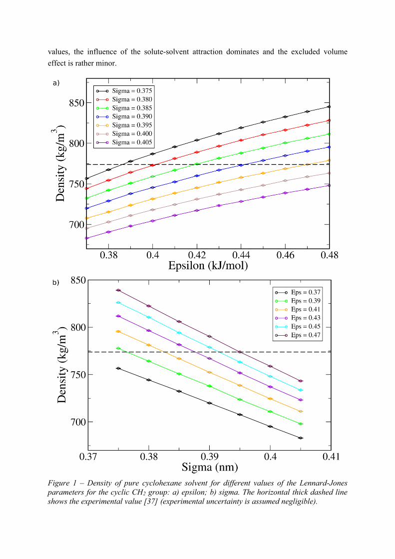
Figure 1 shows that the liquid density decreases linearly with and increases with
in a non-linear fashion within this range of values. Qualitatively speaking, this is expected, as
an increase in increases the excluded volume of each molecule, thus decreasing the density,
while increasing increases the cohesive energy of the fluid, making it denser. Figure 2
shows analogous results for the enthalpy of vaporization. Here we see a practically linear
increase in Hvap with both and in this range of values. Both of these trends are likely to
be caused by an increase in the cohesive energy of the liquid as both and increase (the
increase in excluded volume due to increase in seems to play a negligible role in Hvap).
For the self-solvation free energy (Figure 3), a similar trend as for Hvap is observed,
except that the sign of the gradients is reversed (recall that the vaporization and solvation
processes take place in opposite directions between the gas and liquid/solution phases). The
trend with increasing is once again caused by the stronger solute-solvent interactions, which
favors solvation (i.e., G is more negative). The trend of more favorable solvation with
increasing , however, is not as trivial. It can be rationalized by considering two competing
effects at play: an increase in solute-solvent interactions which is manifested in the increase
of Hvap with ; and an increase in the excluded volume of both solvent and solute
molecules, which is manifested in the decrease of density with . These effects influence G
in opposite ways, since an increase in the volume of the solute will tend to increase the cavity
formation cost, thus making G more positive. However, it appears that within this range of
values, the influence of the solute-solvent attraction dominates and the excluded volume
effect is rather minor.
Figure 1 – Density of pure cyclohexane solvent for different values of the Lennard-Jones
parameters for the cyclic CH2 group: a) epsilon; b) sigma. The horizontal thick dashed line
shows the experimental value [37] (experimental uncertainty is assumed negligible).

Figure 2 – Enthalpy of vaporization of cyclohexane for different values of the Lennard-Jones
parameters for the cyclic CH2 group: a) epsilon; b) sigma. The horizontal thick dashed line
shows the experimental value, while the thin dashed lines represent upper and lower bounds
based on the reported uncertainty in the experimental measurements [38].

Figure 3 – Solvation free energy of cyclohexane solute in cylcohexane solvent (self-solvation)
for different values of the Lennard-Jones parameters for the cyclic CH2 group: a) epsilon; b)
sigma. The horizontal thick dashed line shows the experimental value [18, 19], while the thin
dashed lines represent upper and lower bounds based on the estimated uncertainty in
experimental measurements [40].
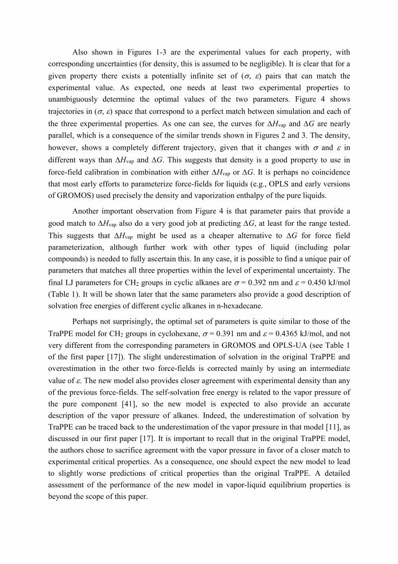
Also shown in Figures 1-3 are the experimental values for each property, with
corresponding uncertainties (for density, this is assumed to be negligible). It is clear that for a
given property there exists a potentially infinite set of (, ) pairs that can match the
experimental value. As expected, one needs at least two experimental properties to
unambiguously determine the optimal values of the two parameters. Figure 4 shows
trajectories in (, ) space that correspond to a perfect match between simulation and each of
the three experimental properties. As one can see, the curves for Hvap and G are nearly
parallel, which is a consequence of the similar trends shown in Figures 2 and 3. The density,
however, shows a completely different trajectory, given that it changes with and in
different ways than Hvap and G. This suggests that density is a good property to use in
force-field calibration in combination with either Hvap or G. It is perhaps no coincidence
that most early efforts to parameterize force-fields for liquids (e.g., OPLS and early versions
of GROMOS) used precisely the density and vaporization enthalpy of the pure liquids.
Another important observation from Figure 4 is that parameter pairs that provide a
good match to Hvap also do a very good job at predicting G, at least for the range tested.
This suggests that Hvap might be used as a cheaper alternative to G for force field
parameterization, although further work with other types of liquid (including polar
compounds) is needed to fully ascertain this. In any case, it is possible to find a unique pair of
parameters that matches all three properties within the level of experimental uncertainty. The
final LJ parameters for CH2 groups in cyclic alkanes are = 0.392 nm and = 0.450 kJ/mol
(Table 1). It will be shown later that the same parameters also provide a good description of
solvation free energies of different cyclic alkanes in n-hexadecane.
Perhaps not surprisingly, the optimal set of parameters is quite similar to those of the
TraPPE model for CH2 groups in cyclohexane, = 0.391 nm and = 0.4365 kJ/mol, and not
very different from the corresponding parameters in GROMOS and OPLS-UA (see Table 1
of the first paper [17]). The slight underestimation of solvation in the original TraPPE and
overestimation in the other two force-fields is corrected mainly by using an intermediate
value of . The new model also provides closer agreement with experimental density than any
of the previous force-fields. The self-solvation free energy is related to the vapor pressure of
the pure component [41], so the new model is expected to also provide an accurate
description of the vapor pressure of alkanes. Indeed, the underestimation of solvation by
TraPPE can be traced back to the underestimation of the vapor pressure in that model [11], as
discussed in our first paper [17]. It is important to recall that in the original TraPPE model,
the authors chose to sacrifice agreement with the vapor pressure in favor of a closer match to
experimental critical properties. As a consequence, one should expect the new model to lead
to slightly worse predictions of critical properties than the original TraPPE. A detailed
assessment of the performance of the new model in vapor-liquid equilibrium properties is
beyond the scope of this paper.
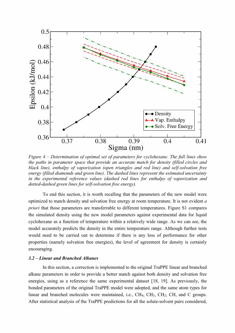
Figure 4 – Determination of optimal set of parameters for cyclohexane. The full lines show
the paths in parameter space that provide an accurate match for density (filled circles and
black line), enthalpy of vaporization (open triangles and red line) and self-solvation free
energy (filled diamonds and green line). The dashed lines represent the estimated uncertainty
in the experimental reference values (dashed red lines for enthalpy of vaporization and
dotted-dashed green lines for self-solvation free energy).
To end this section, it is worth recalling that the parameters of the new model were
optimized to match density and solvation free energy at room temperature. It is not evident a
priori that those parameters are transferrable to different temperatures. Figure S1 compares
the simulated density using the new model parameters against experimental data for liquid
cyclohexane as a function of temperature within a relatively wide range. As we can see, the
model accurately predicts the density in the entire temperature range. Although further tests
would need to be carried out to determine if there is any loss of performance for other
properties (namely solvation free energies), the level of agreement for density is certainly
encouraging.
3.2 – Linear and Branched Alkanes
In this section, a correction is implemented to the original TraPPE linear and branched
alkane parameters in order to provide a better match against both density and solvation free
energies, using as a reference the same experimental dataset [18, 19]. As previously, the
bonded parameters of the original TraPPE model were adopted, and the same atom types for
linear and branched molecules were maintained, i.e., CH4, CH3, CH2, CH, and C groups.
After statistical analysis of the TraPPE predictions for all the solute-solvent pairs considered,

there was nothing to indicate that the deviations from experiment were due to a particular set
of parameters. Instead, deviations were practically independent of the type of sites present in
the solute and solvent molecules. Based on these observations, it was decided to simply
rescale the values of and for all atom types simultaneously (except CH4, see below) by a
constant factor – one scaling factor for and another for . This greatly simplified the
parameterization procedure while still bringing significant improvements in performance
over the entire range of molecular architectures, as will be shown later. It should be noted,
however, that this approach only makes sense because one already has an initial guess of
parameters that is quite close to the optimum (i.e., the original TraPPE parameters). Were this
not the case, and the usual approach of parameterizing each atom type separately would have
to be adopted.
The appropriate scaling factors for and were determined by making use of the
observed variation of and G with those parameters for cyclohexane self-solvation (Figures
1 and 3). In short, the average gradient of change of each property with each parameter was
calculated and then used to estimate the necessary percent change in and that would be
necessary to bring the simulation predictions into agreement with experiment. More
precisely, it was estimated that increasing by 1% and increasing by 2% would cause G
to increase in magnitude (i.e., become more negative) by about 6% and to decrease by
about 1%. The solvation free energy of one solute/solvent pair was then calculated with the
rescaled parameters to test the actual improvement achieved. Nonane in hexadecane was
selected as the training set because this corresponded to one of the largest magnitudes of G,
and because the relative error for the TraPPE model turned out to be nearly identical to the
average relative error of the entire data set, so a good match for this pair is a good indicator
for overall agreement with experiment. Although it was expected that more than one iteration
would be needed, this was not the case – the first guess of the correction factor turned out to
yield excellent agreement for the solvation free energy of nonane in hexadecane. Once again,
this was most likely due to the already good performance of the original TraPPE parameters.
Figures 5, 6, and S1 show how the new parameters (Table 1) lead to an excellent
match between simulation and experiment for linear alkanes dissolved in other linear alkanes.
In particular, the self-solvation of linear alkanes (Figure 6) is in almost perfect agreement
with experiment, which as discussed previously [17] suggests that the vapor pressure of the
pure liquids is also predicted accurately. Moreover, both the density and the enthalpy of
vaporization of pure linear alkane liquids are more accurately predicted by the new model
than by the original TraPPE force-field (Figure 7). The new model is also able to qualitatively
and quantitatively predict the effect of an increase in chain length of the solvent (Figure S2)
and of the solute (Figure 5). Improvements are also significant for linear solutes dissolved in
branched (Figure S3) and cyclic (Figure S4) solvents, as well as for solvation of branched
solutes (Figures S5 and S6).

Figure 5 – Comparison between the original TraPPE model and the new model for linear
alkane solutes of different chain length in n-hexadecane solvent.
Figure 6 – Comparison between the original TraPPE model and the new model for linear
alkane self-solvation (solute and solvent are the same molecule).
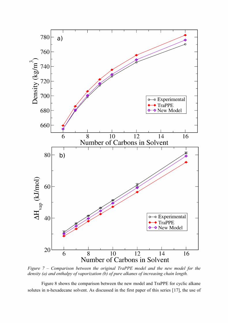
Figure 7 – Comparison between the original TraPPE model and the new model for the
density (a) and enthalpy of vaporization (b) of pure alkanes of increasing chain length.
Figure 8 shows the comparison between the new model and TraPPE for cyclic alkane
solutes in n-hexadecane solvent. As discussed in the first paper of this series [17], the use of
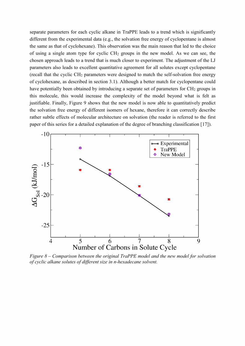
separate parameters for each cyclic alkane in TraPPE leads to a trend which is significantly
different from the experimental data (e.g., the solvation free energy of cyclopentane is almost
the same as that of cyclohexane). This observation was the main reason that led to the choice
of using a single atom type for cyclic CH2 groups in the new model. As we can see, the
chosen approach leads to a trend that is much closer to experiment. The adjustment of the LJ
parameters also leads to excellent quantitative agreement for all solutes except cyclopentane
(recall that the cyclic CH2 parameters were designed to match the self-solvation free energy
of cyclohexane, as described in section 3.1). Although a better match for cyclopentane could
have potentially been obtained by introducing a separate set of parameters for CH2 groups in
this molecule, this would increase the complexity of the model beyond what is felt as
justifiable. Finally, Figure 9 shows that the new model is now able to quantitatively predict
the solvation free energy of different isomers of hexane, therefore it can correctly describe
rather subtle effects of molecular architecture on solvation (the reader is referred to the first
paper of this series for a detailed explanation of the degree of branching classification [17]).
Figure 8 – Comparison between the original TraPPE model and the new model for solvation
of cyclic alkane solutes of different size in n-hexadecane solvent.

Figure 9 – Comparison between the original TraPPE model and the new model for solvation
of hexane isomers of different degree of branching (DoB) in n-hexadecane solvent. The DoB
is 0 for linear molecules, 1 for single-branched molecules, 2 for double-branched molecules
and, rather arbitrarily, -1 for cyclic molecules (see [17] for details).
For all the atom types discussed until now, both and had to be increased relative to
the original TraPPE model to obtain good agreement with experimental solvation free
energies. Methane, however, is an exception – TraPPE actually overestimates the degree of
solvation (i.e., Gsol is less positive than experiment; see Table 1 of the previous paper [17]),
which goes in the opposite direction of the general trend. This means that methane requires a
separate specific parameterization effort. The experimental database of Katritzky et al. [18,
19] contains only a single point for methane (in n-hexadecane), which was considered
insufficient to provide a robust set of parameters. As such, additional data from Wolfenden et
al. [34] for methane solvated in cyclohexane was used. The new parameters for methane were
determined by simultaneously matching the experimental solvation free energy in
cyclohexane and the density of pure methane at its standard boiling point [37], and the
solvation free energy in n-hexadecane was then used for validation of the parameters. Making
use of the trends depicted in Figure 3 for cyclohexane, it was concluded that to match the
solvation free energy a decrease in both and was needed. One started by decreasing by
an initial amount, then found the corresponding value of that provided a close match to the
pure fluid density (iterating in density is more efficient, as the simulations are considerably
faster). This pair of parameters was then tested against the free energy, and a new guess for
was obtained by linear interpolation (i.e., assuming a linear variation of solvation free energy
with both parameters, as shown in Figure 3). The parameters, shown in Table 1, converged

after two iterations. The new parameters lead to very good agreement with the experimental
solvation free energies (absolute deviations of -0.044 kJ/mol for methane in cyclohexane and
0.139 kJ/mol in n-hexadecane) and pure methane density (absolute deviation of 0.4 kg/m3).
To conclude the analysis for alkanes, Figure 10 shows an overall comparison between
experiments and simulations using the new adjusted united-atom model for the entire set of
alkane solute-solvent pairs. Overall statistics are provided in Table 2, in comparison with the
original TraPPE model (for the performance of other UA models, the reader is referred to
Table 2 of the first paper of this series [17]). As can be seen, agreement between simulation
and experiment is excellent across all types of alkane molecules. The relative deviation is
about 1%, while the RMSD is 0.52 kJ/mol, which is within the order of uncertainty in the
experimental data [40].
Table 2 – Measures of deviation between experimental data and simulations using different
models, for the entire alkane data set analyzed: MSD = mean signed deviation; RMSD = root
mean squared deviation.
TraPPE New Model
Slope (fit) 0.940 1.001
R2 (fit) 0.986 0.992
MSD (kJ/mol) -0.967 -0.020
RMSD (kJ/mol) 1.204 0.511
Figure 10 – Comparison between experimental and simulated solvation free energies for the
entire alkane data set using the newly developed force-field. The dashed red line shows a
linear fit (with forced intercept at the origin) through the data. The slope and the correlation
coefficient of the fit are also reported.
3.3 – Alkenes and Alkynes
After establishing that the new model can predict solvation free energies of alkanes to
a high degree of accuracy, the same approach is extended to alkene and alkyne molecules.
Fewer experimental data points [18, 19] are available for those molecules, particularly for the
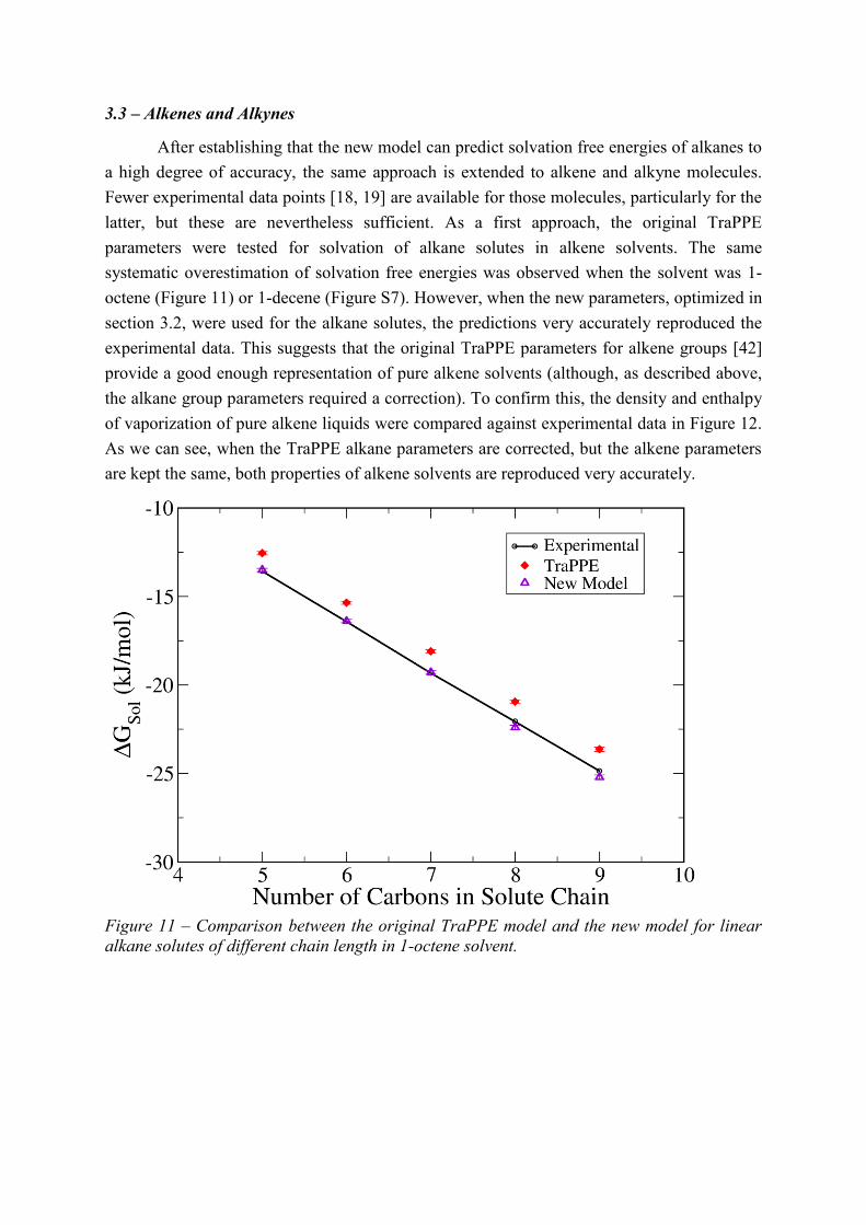
latter, but these are nevertheless sufficient. As a first approach, the original TraPPE
parameters were tested for solvation of alkane solutes in alkene solvents. The same
systematic overestimation of solvation free energies was observed when the solvent was 1-
octene (Figure 11) or 1-decene (Figure S7). However, when the new parameters, optimized in
section 3.2, were used for the alkane solutes, the predictions very accurately reproduced the
experimental data. This suggests that the original TraPPE parameters for alkene groups [42]
provide a good enough representation of pure alkene solvents (although, as described above,
the alkane group parameters required a correction). To confirm this, the density and enthalpy
of vaporization of pure alkene liquids were compared against experimental data in Figure 12.
As we can see, when the TraPPE alkane parameters are corrected, but the alkene parameters
are kept the same, both properties of alkene solvents are reproduced very accurately.
Figure 11 – Comparison between the original TraPPE model and the new model for linear
alkane solutes of different chain length in 1-octene solvent.

Figure 12 – Comparison between experimental data [37, 38] and predictions of the new
model for the density (a) and enthalpy of vaporization (b) of pure alkenes of increasing chain
length. Data are at 298 K except for ethene, propene and 1-butene, which were measured at
their respective boiling points at 1 bar.

As discussed previously, a much more stringent test of model parameters is to predict
solvation free energy of alkene solutes. In Figures 13 and S8, predictions of the TraPPE
model [42] as well as the improved model are compared against experimental data for linear
alkene solutes in n-heptane and n-hexadecane solvents, respectively. Interestingly, the
predictions of the original TraPPE model (i.e., with uncorrected alkane parameters) are quite
close to experiment, although a slight systematic overestimation can be observed for larger
solute molecules. In fact, when predictions of the original TraPPE model are compared
against experimental data for the entire dataset involving alkenes, as either solutes or solvents
(Figure S9), we see the same systematic overestimation reported in the previous paper of this
series for alkanes [17] – solvation free energies are consistently more positive than
experiment – but with a smaller magnitude of deviation (about 4-5% compared to 6% for
pure alkanes). This again suggests that the deficiencies of the TraPPE model are mostly due
to the alkane parameters and not to the alkene parameters.
Figure 13 – Comparison between the original TraPPE model and the new model for linear
alkene solutes of different chain length in n-heptane solvent.
When the alkane parameters are corrected to the values determined in sections 3.1 and
3.2, keeping the alkene parameters the same as in the original TraPPE model, predictions of
alkene solvation are excellent. The exception is solvation of 1-butene in n-hexadecane
(Figure S8), but this is expected to be an error in the experimental data [18, 19], as this point
completely departs from the expected linear trend. In fact, the corresponding value reported
in the Minnesota Solvation Database [35] is -8.49 kJ/mol, which fits within the linear trend
and agrees very well with the new model’s predictions (absolute deviation of -0.102 kJ/mol).
The excellent agreement obtained with the original TraPPE alkene parameters confirms that
no correction to these parameters is needed. As such, the original parameters for alkene
groups were maintained in the new solvation model (Table 1).
The final stage of the new model development was to examine solvation free energies
involving alkynes. Although the polarity of hydrocarbons increases as they become less
saturated, leading some alkenes and alkynes to develop a small dipole moment, a neutral UA
approach was still adopted. Testing the validity of this approximation for solvation in polar
solvents will be the subject of future work. Perhaps surprisingly, it was not possible to find
any UA models of alkynes in the literature (parameters exist for all-atom models, but these
contain explicit hydrogens and point charges, so they are not suitable for our purposes).
Therefore, a new parameter set was developed from scratch, aiming to reproduce solvation
free energies and pure liquid densities of alkyne molecules.
The first step was to determine parameters for CH groups with sp hybridization by
matching the experimental solvation free energy of acetylene in n-heptane [18, 19] and the
density of pure acetylene at its standard boiling point [37]. The parameterization strategy was
very similar to the one described above for methane (section 3.2), except that here one did not
have a good initial guess for the parameters. The line in (, ) parameter space that provided
a good match to the experimental density of acetylene (i.e., the analog of the black line in
Figure 4) was first traced, given that density calculations are computationally cheap. This
focused on a range of values between 0.36 nm and 0.32 nm, as the value of this parameter
is expected to decrease as carbon hybridization increases [11, 42]. Two points on this line
were then selected and two solvation free energy calculations were performed for those pairs
of parameters. Comparing these two results to the target experimental value, a new estimate
of was obtained by linear extrapolation (i.e., assuming linear dependences of free energy
with each of the parameters, as observed in Figure 3). The optimal value of corresponding
to that value of was then obtained by matching the experimental acetylene density, and the
cycle was repeated until convergence. Three iterations were sufficient to obtain the
converged set of parameters shown in Table 1. The validity of the new parameters was
assessed by predicting the solvation free energy of acetylene in n-hexadecane, for which the
deviation was only 0.25 kJ/mol (i.e., well within the precision of experimental data).
Once the CH parameters were found, one moved on to parameterize the C (sp) group.
The experimental database only contained solvation free energies for propyne, 1-butyne, 1-
pentyne and 1-hexyne in n-hexadecane. It was decided to tune the C (sp) parameters to
simultaneously match the density of 1-hexyne and the solvation free energy of propyne in n-
hexadecane. The strategy adopted was identical to the one described above for the CH group,
and converged after three iterations. The quality of the parameters was tested against
solvation free energies, densities and enthalpies of vaporization of the other alkynes. It is
clear from Figure 14 that the new set of parameters yields solvation free energies for the

whole alkyne series in very good agreement with experimental data, which is the main
purpose of the new model. Agreement for density is also good (see Figure 15a) except for 1-
butyne, which shows a deviation of 6.6%, much higher than for any other solvent tested in
this work. Although at present no definitive explanation for this unusual result can be
provided, it is noteworthy that the uncertainties in the density calculations for alkynes larger
than acetylene are quite high. As discussed in section 2, the 180º angle in those molecules led
to unphysical molecular distortions in MD runs with a stochastic dynamics integrator.
Although this problem was subsequently solved, it may have still led to the observed large
amplitude fluctuations in the density of the pure alkynes, and concomitantly large
uncertainties.
Finally, it can be seen in Figure 15b that the enthalpies of vaporization of the alkyne
liquids are systematically underestimated. Although absolute deviations are not very large,
their systematic nature may represent an inherent limitation of the united-atom approach for
alkynes. Further work is necessary to fully ascertain this. Arguably, it may have been
possible to tune the parameters for CH and C groups simultaneously to provide the best
compromise in fitting the densities, enthalpies of vaporization and solvation free energies for
all the molecules studied. However, because the target experimental data is quite limited and
because of the technical issued discussed above, this was not pursued any further.
Figure 14 – Comparison between experimental data and predictions of the new model for
linear alkyne solutes of different chain length in n-hexadecane solvent.

Figure 15 – Comparison between experimental data [37, 38] and predictions of the new
model for the density (a) and enthalpy of vaporization (b) of pure alkynes of increasing chain
length. Data are at 293 K except for acetylene, propyne and 1-butyne, which are at their
respective boiling temperatures.

Figure 16 compares the predictions of the new model against experimental data for
the entire data set involving alkenes and alkynes [18, 19] (which also contain alkane groups,
as discussed above). It is clear that the new model yields predictions in excellent agreement
with experimental data for the entire dataset, with the exception of two outliers: 1-butene in
n-hexadecane and 1-pentene in 2,2,4-trimethylpentane. The former was discussed above and
is believed to be an error in the experimental data (the value reported in the Minesotta
Solvation Database [35] is actually much closer to our predictions). For the latter, however,
the Minesotta Solvation Database [35] reports a value (-9.87 kJ/mol) that is almost identical
to that of Katritzky et al. [18, 19]. At present, the origin of this discrepancy is not completely
understood, and further tests (both experimental and theoretical) are required. Overall, even
including the two outliers, the mean signed deviation from experimental data is 0.17 kJ/mol,
corresponding to a relative deviation of about 1%, and the RMSD is only 0.68 kJ/mol, again
well within the experimental uncertainty [40].
Figure 16 – Comparison between experimental and simulated solvation free energies for the
entire alkene and alkyne data set using the newly developed force-field. The dashed red line
shows a linear fit (with forced intercept at the origin) through the data. The slope and the
correlation coefficient of the fit are also reported.
4 - Conclusions
In this paper a new fully transferrable united-atom model for hydrocarbon molecules
that is able to accurately predict hydrophobic solvation free energies (i.e., solvation of
hydrocarbons in other hydrocarbons) has been presented. The starting point for the
parameterization was the TraPPE force-field, as it has been shown in the previous paper of
this series that it performs best among several popular UA models. Accurate solvation free
energy predictions of linear and branched alkanes were obtained by implementing a small
correction to the original TraPPE parameters for CH3, CH2, CH and C sites with sp3
hybridization (increasing by 1% and by 2%). Methane parameters, however, required a
small correction (below 1% for both and ) in the opposite direction. A new set of
parameters for CH2 groups in cyclic alkanes that is applicable to all molecules of this type has
also been developed. These changes were able to correct the systematic underestimation of
alkane solvation free energies observed for the TraPPE model, while simultaneously yielding
a better description of pure fluid densities. The new alkane parameters also led to excellent
predictions of alkene solvation free energies, when combined with the original TraPPE
parameters for CH2 (sp2) and CH (sp2) sites. For this reason, the parameters for sp2 sites were
kept unchanged in the new model. Finally, a new set of parameters for sites with sp
hybridization has been proposed, which led to accurate predictions of solvation free energies
and densities of alkynes. Averaging over the entire data set comprising 95 solute/solvent
pairs, the mean signed deviation between experiments and simulations using the new model
is 0.064 kJ/mol, while the RMSD is only 0.6 kJ/mol. The latter is below the estimated
uncertainty of 0.8 kJ/mol in the experimental measurements. This new set of parameters
represents an improvement over previous models and is a solid base for development of a
classical non-polarizable force-field that is able to accurately predict solvation free energies
in both polar and non-polar solvents. Extension of this model to describe polar compounds
requires, of course, consideration of electrostatic interactions. Further work in this direction is
currently underway.
Supplementary Material
Additional results figures, as detailed in the main text; full table with all experimental and
simulated solvation free energies, full tables of interaction parameters of the new model.
Input files for all solvation free energy calculations are freely available from the University of
Strathclyde’s data repository (DOI: 10.15129/1bd18245-1226-42ed-84d9-48ae37e3d765).
Acknowledgements
The author would like to thank the volunteer computing platform IBERCIVIS for all the
assistance provided during the implementation and execution of project SOLUVEL. Javier
Palacios Ramos, Francisco Sanz García, Carlos Simões, Cândida Silva and Rui Brito deserve
a special mention for their tireless support. IBERCIVIS was supported in part by grants from

UMIC (Agência para a Sociedade do Conhecimento) and FCT (Fundação para a Ciência e a
Tecnologia) in Portugal, and the IBERCIVIS foundation, CSIC (Consejo Superior de
Investigaciones Cientificas) and Gobierno de Aragon in Spain. Special thanks are due to all
the volunteers that contributed with their time and computer resources to the IBERCIVIS
network.
References
[1] Westergren, J.; Lindfors, L.; Höglund, T.; Lüder, K.; Nordholm, S.; Kjellander, R.; In
silico prediction of drug solubility: 1. Free energy of hydration. J. Phys. Chem. B 2007, 111,
1872-1882.
[2] Garrido, N. M.; Queimada, A. J.; Jorge, M.; Macedo, E. A.; Economou, I. G. 1-
Octanol/Water Partition Coefficients of n-Alkanes from Molecular Simulations of Absolute
Solvation Free Energies. J. Chem. Theory Comput, 2009 5, 2436-2446.
[3] Rao, S. N.; Singh, U. C.; Bash, P. A.; Kollman, P. A. Free energy perturbation
calculations on binding and catalysis after mutating Asn 155 in subtilisin. Nature 1987, 328,
551-554.
[4] Kollman, P. Free energy calculations: Applications to chemical and biochemical
phenomena. Chem. Rev. 1993, 93, 2395-2417.
[5] Mobley, D. L.; Bayly, C. I.; Cooper, M. D.; Shirts, M. R.; Dill, K. A. Small molecule
hydration free energies in explicit solvent: An extensive test of fixed-charge atomistic
simulations. J. Chem. Theory Comput. 2009, 5, 350–358.
[6] Shivakumar, D.; Williams, J.; Wu, Y.; Damm, W.; Shelley, J.; Sherman, W. Predicition of
absolute solvation free energies using molecular dynamics free energy perturbation and the
OPLS force field. J. Chem. Theory Comput. 2010, 6, 1509–1519.
[7] Knight, J. L.; Yesselman, J. D.; Brooks, III, C. L. Assessing the quality of absolute
hydration free energies among the CHARMM-compatible ligand parametrization schemes. J.
Comput. Chem. 2013, 34, 893–903.
[8] Jorgensen, W. L.; Tirado–Rives, J. The OPLS potential functions for proteins. Energy
minimizations for crystals of cyclic peptides and crambin. J. Am. Chem. Soc. 1988, 110,
1657-1666.
[9] Oostenbrink, C.; Villa, A.; Mark, A. E.; van Gunsteren, W. F. A biomolecular force field
based on the free enthalpy of hydration and solvation: the GROMOS force-field parameter
sets 53A5 and 53A6. J. Comput. Chem. 2004, 25, 1656-1676.
[10] Schuler, L. D.; Daura, X.; van Gunsteren, W. F. An improved GROMOS96 force field
for aliphatic hydrocarbons in the condensed phase. J. Comput. Chem. 2001, 22, 1205–1218.
[11] Martin, M. G.; Siepmann, J. I. Transferable potentials for phase equilibria. 1. United-
atom description of n –alkanes. J. Phys. Chem. B 1998, 102, 2569-2577.

[12] Martin, M. G.; Siepmann, J. I. Novel configurational-bias Monte Carlo method for
branched molecules. Transferable potentials for phase equilibria. 2. United-atom description
of branched alkanes. J. Phys. Chem. B 1999, 103, 4508-4517.
[13] Lee, J.-S.; Wick, C. D.; Stubbs, J. M.; Siepmann, J. I. Simulating the vapour–liquid
equilibria of large cyclic alkanes. Mol. Phys. 2005, 103, 99−104.
[14] Keasler, S. J.; Charan, S. M.; Wick, C. D.; Economou, I. G.; Siepmann, J. I. Transferable
Potentials for Phase Equilibria−United Atom Description of Five- and Six-Membered Cyclic
Alkanes and Ethers. J. Phys. Chem. B 2012, 116, 11234−11246.
[15] Dysthe, D. K.; Fuchs, A. H.; Rousseau, B. Fluid transport properties by equilibrium
molecular dynamics. III. Evaluation of united atom interaction potential models for pure
alkanes. J. Chem. Phys. 2000, 112, 7581-7590.
[16] Leontyev, I.; Stuchebrukhov, A. A. Electronic Continuum Model for Molecular
Dynamics Simulations. J. Chem. Phys. 2009, 130, 085102.
[17] Jorge, M.; Garrido, N. M.; Predicting Hydrophobic Solvation by Molecular Simulation:
1. Testing United-atom Alkane Models. Submitted.
[18] Katritzky, A. R.; Oliferenko, A. A.; Oliferenko, P. V.; Petrukhin, R.; Tatham, D. B.;
Maran, U.; Lomaka, A.; Acree, W. E. Jr. A General Treatment of Solubility. 1. The QSPR
Correlation of Solvation Free Energies of Single Solutes in Series of Solvents. J. Chem. Inf.
Comput. Sci. 2003, 43, 1794–1805.
[19] Katritzky, A. R.; Tulp, I.; Fara, D. C.; Lauria, A.; Maran, U.; Acree, W. E. Jr. A General
Treatment of Solubility. 3. Principal Component Analysis (PCA) of the Solubilities of
Diverse Solutes in Diverse Solvents. J. Chem. Inf. Model. 2005, 45, 913–923.
[20] Garrido, N. M.; Jorge, M., Queimada, A. J.; Macedo, E. A.; Economou, I. G. Using
Molecular Simulation to Predict Solute Solvation and Partition Coefficients in Solvents of
Different Polarity. Phys. Chem. Chem. Phys. 2011, 13, 9155-9164.
[21] Garrido, N. M.; Jorge, M.; Queimada, A. J.; Economou, I. G.; Macedo, E. A. Molecular
Simulation of the Hydration Gibbs Energy of Barbiturates. Fluid Phase Equilibr., 2010, 289,
148-155.
[22] Garrido, N. M.; Queimada, A. J.; Jorge, M.; Economou, I. G.; Macedo, E. A. Molecular
Simulation of Absolute Hydration Gibbs Energies of Polar Compounds. Fluid Phase
Equilibr., 2010, 296, 110-115.
[23] Garrido, N. M.; Jorge, M.; Queimada, A. J.; Gomes, J. R. B.; Economou, I. G.; Macedo,
E. A. Predicting hydration Gibbs energies of alkyl-aromatics using molecular simulation: a
comparison of current force fields and the development of a new parameter set for accurate
solvation data. Phys. Chem. Chem. Phys., 2011, 13, 17384-17394.
[24] Garrido, N. M.; Queimada, A. J.; Jorge, M.; Economou, I. G.; Macedo, E. A. Prediction
of the n-hexane/water and 1-octanol/water Partition Coefficients for Environmentally
Relevant Compounds using Molecular Simulation. AIChE J. 2012, 58, 1929-1938.
[25] Jorge, M.; Garrido, N. M.; Queimada, A. J.; Economou, I. G.; Macedo, E. A. Effect of
the Integration Method on the Accuracy and Computational Efficiency of Free Energy
Calculations Using Thermodynamic Integration. J. Chem. Theory Comput. 2010, 6, 1018-
1027.
[26] Kirkwood, J. G.; Statistical mechanics of fluid mixtures. J. Chem. Phys. 1935, 3, 300-
313.
[27] Hess, B.; Kutzner, C.; van der Spoel, D.; Lindahl, E. GROMACS 4: Algorithms for
Highly Efficient, Load-Balanced, and Scalable Molecular Simulation. J. Chem. Theory
Comput. 2008, 4, 435–447.
[28] http://www.IBERCIVIS.com/
[29] van Gunsteren, W. F.; Berendsen, H. J. C. Algorithms for Brownian Dynamics. Mol.
Phys. 1982, 45, 637–647.
[30] Parrinello, M.; Rahman, A. Crystal Structure and Pair Potentials: A Molecular-
Dynamics Study. Phys. Rev. Lett. 1980, 45, 1196-1199.
[31] van Gunsteren, W.; Berendsen, H. A leap-frog algorithm for stochastic dynamics. Mol.
Simul. 1988, 1, 173–185.
[32] Paliwal, H.; Shirts, M. R. Using multistate reweighting to rapidly and efficiently explore
molecular simulation parameters space for nonbonded interactions. J. Chem. Theory Comput.
2013, 9, 4700-4717.
[33] Jorgensen, W. L; Maxwell, D. S; Tirado-Rives, J. Development and Testing of the OPLS
All-Atom Force Field on Conformational Energetics and Properties of Organic Liquids. J.
Am. Chem. Soc. 1996, 118, 11225–11236.
[34] Radzicka, A.; Wolfenden, R. Comparing the polarities of the amino acids: side-chain
distribution coefficients between the vapor phase, cyclohexane, 1-octanol, and neutral
aqueous solution. Biochemistry 1988, 27, 1664-1670.
[35] Marenich, A. V.; Kelly, C. P.; Thompson, J. D.; Hawkins, G. D.; Chambers, C. C.;
Giesen, D. J.; Winget, P.; Cramer, C. J.; Truhlar, D. G. Minnesota Solvation Database –
version 2012, University of Minnesota, Minneapolis, 2012.
[36] Marenich, A. V.; Olson, R. M.; Kelly, C. P.; Cramer, C. J.; Truhlar, D. G. Self-
consistent reaction field model for aqueous and nonaqueous solutions based on accurate
polarized partial charges. J. Chem. Theory Comput. 2007, 3, 2011-2033.
[37] Weast, R. C.; Astle, M. J. Handbook of Data on Organic Compounds. CRC Press: Boca
Raton (Fla.), USA, 1985.
[38] NIST Chemistry webbook, http://webbook.nist.gov/chemistry/, accessed 16/10/2016.
[39] Errington, J. R.; Panagiotopoulos, A. Z. New intermolecular potential models for
benzene and cyclohexane. J. Chem. Phys. 1999, 111, 9731−9738.
[40] Li, J.; Zhu, T.; Hawkins, G. D.; Winget, P.; Liotard, D. A.; Cramer, C. J.; Truhlar, D. G.
Extension of the Platform of Applicability of the SM5.42R Universal Solvation Model.
Theor. Chem. Acc. 1999, 103, 9-63.
[41] Winget, P.; Hawkins, G. D.; Cramer, C. J.; Truhlar, D. G. Prediction of Vapor Pressures
from Self-Solvation Free Energies Calculated by the SM5 Series of Universal Solvation
Models. J. Phys. Chem. B 2000, 104, 4726-4734.
[42] Wick, C. D.; Martin, M. G.; Siepmann, J. I. Transferable potentials for phase equilibria.
4. United-atom description of linear and branched alkenes and alkylbenzenes. J. Phys. Chem.
B 2000, 104, 8008.
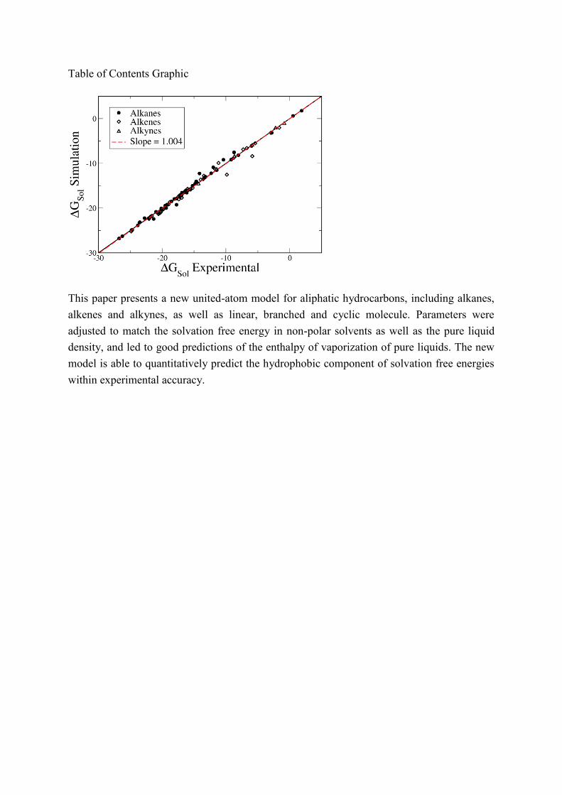
Table of Contents Graphic
This paper presents a new united-atom model for aliphatic hydrocarbons, including alkanes,
alkenes and alkynes, as well as linear, branched and cyclic molecule. Parameters were
adjusted to match the solvation free energy in non-polar solvents as well as the pure liquid
density, and led to good predictions of the enthalpy of vaporization of pure liquids. The new
model is able to quantitatively predict the hydrophobic component of solvation free energies
within experimental accuracy.

SUPPLEMENTARY MATERIAL
Predicting Hydrophobic Solvation by Molecular Simulation: 2.
New United-atom Model for Alkanes, Alkenes and Alkynes
Miguel Jorge*
Department of Chemical and Process Engineering, University of Strathclyde, 75 Montrose Street,
Glasgow G1 1XJ, United Kingdom
Email – [email protected]
S1 – Computational Methods
For the alkane and alkene models, we have used the bonded parameters of the TraPPE force
field. Unfortunately, no bonded parameters were available for alkynes in this force field. As such, we
have used the bonded parameters of the OPLS-AA force field, which are provided in Table S1.
Table S1 – Bonded parameters for alkynes1, taken from the OPLS-AA force field [1]. The torsional
potentials around bonds involving alkyne atoms are all zero in this model.
Bond Stretching l (nm) Kl (kJ.mol-1.nm-2)
CZ-CZ 0.121 962320
CZ-CT 0.147 326352
Angle Bending (deg) K (kJ.mol-1.rad-2)
CZ-CZ-CT 180 1255.2
CZ-CT-CT 112.7 488.273 1 CZ denotes a group with sp hybridization, while CT denotes an sp3 group.
Non-bonded interactions were modeled by the Lennard-Jones (LJ) potential:
612
4ij
ij
ij
ij
ijijrr
E
(S1)
where rij is the distance between two LJ interaction sites. To determine values of ij and ij for
interaction between different atom types (i.e., cross interactions), we applied the Lorentz-Berthelot
combination rules. For completeness, we provide all cross-interaction parameters in Tables S2 and
S3. The LJ potential can also be expressed in terms of constants C12 and C6, which can be easily
calculated from the tables of and according to the following relations:
6
6
12
12 4;4 CC (S2)
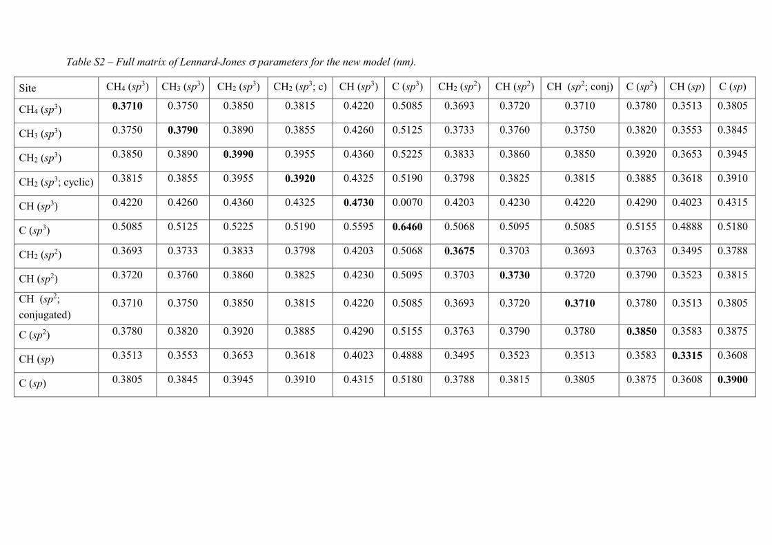
Table S2 – Full matrix of Lennard-Jones parameters for the new model (nm).
Site CH4 (sp3) CH3 (sp3) CH2 (sp3) CH2 (sp3; c) CH (sp3) C (sp3) CH2 (sp2) CH (sp2) CH (sp2; conj) C (sp2) CH (sp) C (sp)
CH4 (sp3) 0.3710 0.3750 0.3850 0.3815 0.4220 0.5085 0.3693 0.3720 0.3710 0.3780 0.3513 0.3805
CH3 (sp3) 0.3750 0.3790 0.3890 0.3855 0.4260 0.5125 0.3733 0.3760 0.3750 0.3820 0.3553 0.3845
CH2 (sp3) 0.3850 0.3890 0.3990 0.3955 0.4360 0.5225 0.3833 0.3860 0.3850 0.3920 0.3653 0.3945
CH2 (sp3; cyclic) 0.3815 0.3855 0.3955 0.3920 0.4325 0.5190 0.3798 0.3825 0.3815 0.3885 0.3618 0.3910
CH (sp3) 0.4220 0.4260 0.4360 0.4325 0.4730 0.0070 0.4203 0.4230 0.4220 0.4290 0.4023 0.4315
C (sp3) 0.5085 0.5125 0.5225 0.5190 0.5595 0.6460 0.5068 0.5095 0.5085 0.5155 0.4888 0.5180
CH2 (sp2) 0.3693 0.3733 0.3833 0.3798 0.4203 0.5068 0.3675 0.3703 0.3693 0.3763 0.3495 0.3788
CH (sp2) 0.3720 0.3760 0.3860 0.3825 0.4230 0.5095 0.3703 0.3730 0.3720 0.3790 0.3523 0.3815
CH (sp2;
conjugated) 0.3710 0.3750 0.3850 0.3815 0.4220 0.5085 0.3693 0.3720 0.3710 0.3780 0.3513 0.3805
C (sp2) 0.3780 0.3820 0.3920 0.3885 0.4290 0.5155 0.3763 0.3790 0.3780 0.3850 0.3583 0.3875
CH (sp) 0.3513 0.3553 0.3653 0.3618 0.4023 0.4888 0.3495 0.3523 0.3513 0.3583 0.3315 0.3608
C (sp) 0.3805 0.3845 0.3945 0.3910 0.4315 0.5180 0.3788 0.3815 0.3805 0.3875 0.3608 0.3900

Table S3 – Full matrix of Lennard-Jones parameters for the new model (kJ/mol).
Site CH4 (sp3) CH3 (sp3) CH2 (sp3) CH2 (sp3; c) CH (sp3) C (sp3) CH2 (sp2) CH (sp2) CH (sp2; conj) C (sp2) CH (sp) C (sp)
CH4 (sp3) 1.2000 0.9998 0.6859 0.7348 0.3194 0.0715 0.9209 0.6848 0.7203 0.4467 0.8681 0.6753
CH3 (sp3) 0.9998 0.8330 0.5714 0.6122 0.2661 0.0596 0.7673 0.5705 0.6001 0.3722 0.7233 0.5626
CH2 (sp3) 0.6859 0.5714 0.3920 0.4200 0.1825 0.0409 0.5263 0.3914 0.4117 0.2553 0.4962 0.3860
CH2 (sp3; cyclic) 0.7348 0.6122 0.4200 0.4500 0.1956 0.0438 0.5639 0.4193 0.4411 0.2735 0.5316 0.4135
CH (sp3) 0.3194 0.2661 0.1825 0.1956 0.0850 0.0070 0.2451 0.1822 0.1917 0.1189 0.2310 0.1797
C (sp3) 0.0715 0.0596 0.0409 0.0438 0.0190 0.0043 0.0549 0.0408 0.0429 0.0266 0.0517 0.0402
CH2 (sp2) 0.9209 0.7673 0.5263 0.5639 0.2451 0.0549 0.7067 0.5255 0.5527 0.3428 0.6662 0.5182
CH (sp2) 0.6848 0.5705 0.3914 0.4193 0.1822 0.0408 0.5255 0.3908 0.4110 0.2549 0.4954 0.3853
CH (sp2;
conjugated) 0.7203 0.6001 0.4117 0.4411 0.1917 0.0429 0.5527 0.4110 0.4323 0.2681 0.5211 0.4053
C (sp2) 0.4467 0.3722 0.2553 0.2735 0.1189 0.0266 0.3428 0.2549 0.2681 0.1663 0.3231 0.2514
CH (sp) 0.8681 0.7233 0.4962 0.5316 0.2310 0.0517 0.6662 0.4954 0.5211 0.3231 0.6280 0.4885
C (sp) 0.6753 0.5626 0.3860 0.4135 0.1797 0.0402 0.5182 0.3853 0.4053 0.2514 0.4885 0.3800

S2 – Force-field Validation
Figure S1 – Density of pure cyclohexane as a function of temperature from experiment (black line)
and simulations using the new model developed in this work (red circles).
Figure S2 – Comparison between the original TraPPE model and the new model for solvation of n-
hexane solute in linear alkane solvents of different chain length.

Figure S3 – Comparison between the original TraPPE model and the new model for linear alkane
solutes of different chain length in 2,2,4-trimethylpentane solvent.
Figure S4 – Comparison between the original TraPPE model and the new model for linear alkane
solutes of different chain length in cyclohexane solvent.
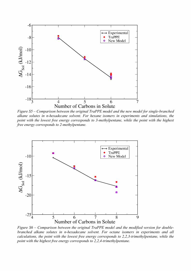
Figure S5 – Comparison between the original TraPPE model and the new model for single-branched
alkane solutes in n-hexadecane solvent. For hexane isomers in experiments and simulations, the
point with the lowest free energy corresponds to 3-methylpentane, while the point with the highest
free energy corresponds to 2-methylpentane.
Figure S6 – Comparison between the original TraPPE model and the modified version for double-
branched alkane solutes in n-hexadecane solvent. For octane isomers in experiments and all
calculations, the point with the lowest free energy corresponds to 2,2,3-trimethylpentane, while the
point with the highest free energy corresponds to 2,2,4-trimethylpentane.
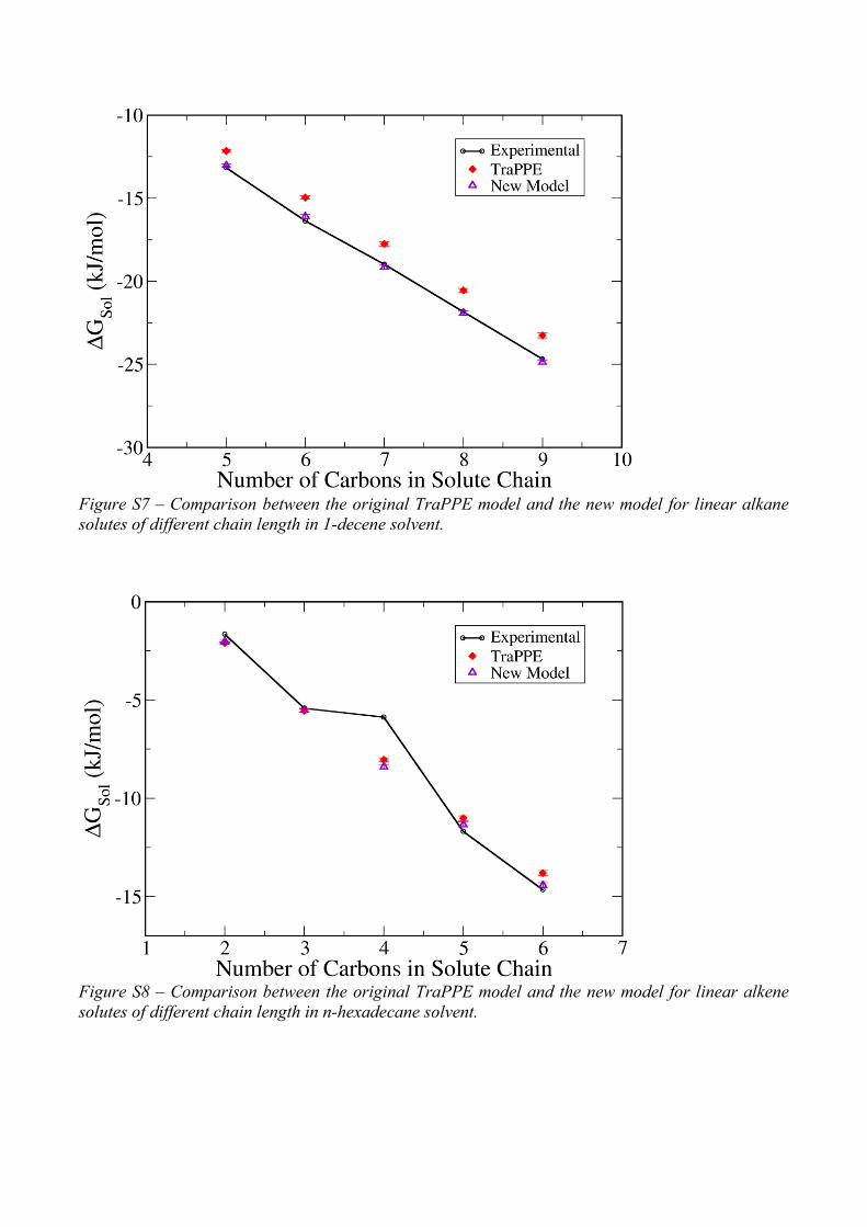
Figure S7 – Comparison between the original TraPPE model and the new model for linear alkane
solutes of different chain length in 1-decene solvent.
Figure S8 – Comparison between the original TraPPE model and the new model for linear alkene
solutes of different chain length in n-hexadecane solvent.

Figure S9 – Comparison between experimental and simulated solvation free energies for the entire
alkene data set using the TraPPE force-field. The dashed red line shows a linear fit (with forced
intercept at the origin) through the data. We report also the slope and the correlation coefficient of
the fit.

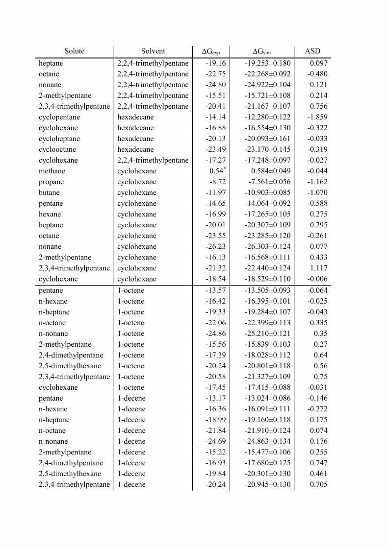
Table S4 – Comparison between experimental solvation free energies and those calculated using the
new model for the entire data set of alkanes, alkenes and alkynes examined in this paper. All values
are in kJ/mol. Experimental data are from refs [1] and [2], except where noted. Uncertainty in the
simulated free energies is reported as ± the standard error. ASD = absolute signed deviation
between simulation and experiment. The first section includes pairs involving only alkanes, the
second section includes pairs that involve at least one alkene, and the third section includes pairs
that involve at least one alkyne.
Solute Solvent Gexp Gsim ASD
methane hexadecane 1.88 1.744±0.064 0.139
ethane hexadecane -2.80 -3.175±0.076 0.372
propane hexadecane -5.98 -6.117±0.094 0.134
butane hexadecane -9.16 -9.184±0.113 0.021
pentane hexadecane -12.30 -12.230±0.125 -0.071
hexane hexadecane -15.23 -15.026±0.143 -0.204
heptane hexadecane -18.07 -17.969±0.148 -0.106
octane hexadecane -20.96 -20.849±0.167 -0.113
nonane hexadecane -23.81 -23.883±0.163 0.076
decane hexadecane -26.74 -26.803±0.585 0.067
hexane hexane -16.88 -16.824±0.090 -0.052
hexane heptane -16.53 -16.515±0.096 -0.019
hexane octane -16.31 -16.444±0.100 0.138
hexane nonane -16.13 -16.110±0.102 -0.025
hexane decane -15.96 -16.058±0.109 0.094
hexane dodecane -15.56 -15.807±0.121 0.242
heptane heptane -19.50 -19.462±0.097 -0.036
octane octane -22.12 -22.310±0.122 0.189
nonane nonane -24.69 -24.960±0.136 0.273
isobutane hexadecane -8.03 -8.203±0.064 0.170
isopentane hexadecane -11.46 -11.530±0.076 0.066
neopentane hexadecane -10.38 -9.214±0.094 -1.162
2-methylpentane hexadecane -14.54 -14.361±0.116 -0.177
3-methylpentane hexadecane -14.82 -14.574±0.125 -0.249
2,2-dimethylbutane hexadecane -13.23 -13.036±0.133 -0.191
2,3-dimethylpentane hexadecane -17.22 -17.386±0.139 0.168
2,2,3-trimethylbutane hexadecane -16.23 -16.174±0.145 -0.060
2,3,4-trimethylpentane hexadecane -19.38 -20.006±0.139 0.622
2,2,4-trimethylpentane hexadecane -17.73 -17.885±0.153 0.154
2,2,3-trimethylpentane hexadecane -17.74 -19.263±0.157 1.523
pentane 2,2,4-trimethylpentane -13.40 -13.272±0.178 -0.126
hexane 2,2,4-trimethylpentane -16.31 -16.156±0.192 -0.150
Solute Solvent Gexp Gsim ASD
heptane 2,2,4-trimethylpentane -19.16 -19.253±0.180 0.097
octane 2,2,4-trimethylpentane -22.75 -22.268±0.092 -0.480
nonane 2,2,4-trimethylpentane -24.80 -24.922±0.104 0.121
2-methylpentane 2,2,4-trimethylpentane -15.51 -15.721±0.108 0.214
2,3,4-trimethylpentane 2,2,4-trimethylpentane -20.41 -21.167±0.107 0.756
cyclopentane hexadecane -14.14 -12.280±0.122 -1.859
cyclohexane hexadecane -16.88 -16.554±0.130 -0.322
cycloheptane hexadecane -20.13 -20.093±0.161 -0.033
cyclooctane hexadecane -23.49 -23.170±0.145 -0.319
cyclohexane 2,2,4-trimethylpentane -17.27 -17.248±0.097 -0.027
methane cyclohexane 0.54* 0.584±0.049 -0.044
propane cyclohexane -8.72 -7.561±0.056 -1.162
butane cyclohexane -11.97 -10.903±0.085 -1.070
pentane cyclohexane -14.65 -14.064±0.092 -0.588
hexane cyclohexane -16.99 -17.265±0.105 0.275
heptane cyclohexane -20.01 -20.307±0.109 0.295
octane cyclohexane -23.55 -23.285±0.120 -0.261
nonane cyclohexane -26.23 -26.303±0.124 0.077
2-methylpentane cyclohexane -16.13 -16.568±0.111 0.433
2,3,4-trimethylpentane cyclohexane -21.32 -22.440±0.124 1.117
cyclohexane cyclohexane -18.54 -18.529±0.110 -0.006
pentane 1-octene -13.57 -13.505±0.093 -0.064
n-hexane 1-octene -16.42 -16.395±0.101 -0.025
n-heptane 1-octene -19.33 -19.284±0.107 -0.043
n-octane 1-octene -22.06 -22.399±0.113 0.335
n-nonane 1-octene -24.86 -25.210±0.121 0.35
2-methylpentane 1-octene -15.56 -15.839±0.103 0.27
2,4-dimethylpentane 1-octene -17.39 -18.028±0.112 0.64
2,5-dimethylhexane 1-octene -20.24 -20.801±0.118 0.56
2,3,4-trimethylpentane 1-octene -20.58 -21.327±0.109 0.75
cyclohexane 1-octene -17.45 -17.415±0.088 -0.031
pentane 1-decene -13.17 -13.024±0.086 -0.146
n-hexane 1-decene -16.36 -16.091±0.111 -0.272
n-heptane 1-decene -18.99 -19.160±0.118 0.175
n-octane 1-decene -21.84 -21.910±0.124 0.074
n-nonane 1-decene -24.69 -24.863±0.134 0.176
2-methylpentane 1-decene -15.22 -15.477±0.106 0.255
2,4-dimethylpentane 1-decene -16.93 -17.680±0.125 0.747
2,5-dimethylhexane 1-decene -19.84 -20.301±0.130 0.461
2,3,4-trimethylpentane 1-decene -20.24 -20.945±0.130 0.705

Solute Solvent Gexp Gsim ASD
cyclohexane 1-decene -17.22 -17.093±0.098 -0.125
ethene n-heptane -2.96 -3.179±0.055 0.214
propylene n-heptane -7.30 -6.873±0.064 -0.425
1-hexene n-heptane -16.02 -15.711±0.086 -0.310
1-heptene n-heptane -18.81 -18.653±0.097 -0.161
1-octene n-heptane -21.61 -21.744±0.106 0.136
1,3-butadiene n-heptane -11.17 -9.926±0.070 -1.249
2-methyl-2-butene n-heptane -13.97 -13.634±0.085 -0.334
isoprene n-heptane -13.46 -12.772±0.079 -0.683
propylene 2,2,4-trimethylpentane -6.73 -6.597±0.066 -0.131
1-pentene 2,2,4-trimethylpentane -9.86 -12.521±0.093 2.658
ethene hexadecane -1.65 -2.025±0.069 0.372
propylene hexadecane -5.42 -5.519±0.096 0.103
1-butene hexadecane -5.87 -8.388±0.105 2.516
1-pentene hexadecane -11.69 -11.337±0.127 -0.351
1-hexene hexadecane -14.65 -14.418±0.128 -0.234
1,3-butadiene hexadecane -8.78 -8.763±0.099 -0.017
acetylene hexadecane -0.86 -1.102±0.060 0.247
propyne hexadecane -5.87 -5.786±0.097 -0.086
1-butyne hexadecane -8.67 -8.733±0.106 0.067
1-pentyne hexadecane -11.46 -11.460±0.129 0.000
1-hexyne hexadecane -14.31 -14.639±0.143 0.329
acetylene n-heptane -2.22 -2.138±0.046 -0.086
* Taken from ref [3]
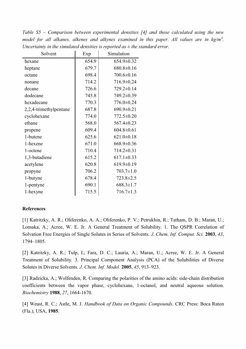
Table S5 – Comparison between experimental densities [4] and those calculated using the new
model for all alkanes, alkenes and alkynes examined in this paper. All values are in kg/m3.
Uncertainty in the simulated densities is reported as ± the standard error.
Solvent Exp Simulation
hexane 654.9 654.9±0.32
heptane 679.7 680.8±0.16
octane 698.4 700.6±0.16
nonane 714.2 716.9±0.24
decane 726.6 729.2±0.14
dodecane 745.8 749.2±0.39
hexadecane 770.3 776.0±0.24
2,2,4-trimethylpentane 687.8 690.9±0.21
cyclohexane 774.0 772.5±0.20
ethane 568.0 567.4±0.23
propene 609.4 604.8±0.61
1-butene 625.6 621.0±0.18
1-hexene 671.0 668.9±0.36
1-octene 710.4 714.2±0.31
1,3-butadiene 615.2 617.1±0.33
acetylene 620.8 619.9±0.19
propyne 706.2 703.7±1.0
1-butyne 678.4 723.8±2.5
1-pentyne 690.1 688.3±1.7
1-hexyne 715.5 716.7±1.3
References
[1] Katritzky, A. R.; Oliferenko, A. A.; Oliferenko, P. V.; Petrukhin, R.; Tatham, D. B.; Maran, U.;
Lomaka, A.; Acree, W. E. Jr. A General Treatment of Solubility. 1. The QSPR Correlation of
Solvation Free Energies of Single Solutes in Series of Solvents. J. Chem. Inf. Comput. Sci. 2003, 43,
1794–1805.
[2] Katritzky, A. R.; Tulp, I.; Fara, D. C.; Lauria, A.; Maran, U.; Acree, W. E. Jr. A General
Treatment of Solubility. 3. Principal Component Analysis (PCA) of the Solubilities of Diverse
Solutes in Diverse Solvents. J. Chem. Inf. Model. 2005, 45, 913–923.
[3] Radzicka, A.; Wolfenden, R. Comparing the polarities of the amino acids: side-chain distribution
coefficients between the vapor phase, cyclohexane, 1-octanol, and neutral aqueous solution.
Biochemistry 1988, 27, 1664-1670.
[4] Weast, R. C.; Astle, M. J. Handbook of Data on Organic Compounds. CRC Press: Boca Raton
(Fla.), USA, 1985.

Related Documents