Predicting General Aviation Accident Frequency From Pilot Total Flight Hours William R. Knecht FAA Civil Aerospace Medical Institute Federal Aviation Administration Oklahoma City, OK 73125 October 2012 Final Report DOT/FAA/AM-12/15 Office of Aerospace Medicine Washington, DC 20591 Federal Aviation Administration

Welcome message from author
This document is posted to help you gain knowledge. Please leave a comment to let me know what you think about it! Share it to your friends and learn new things together.
Transcript
Predicting General Aviation Accident Frequency From Pilot Total Flight Hours
William R. KnechtFAA Civil Aerospace Medical InstituteFederal Aviation AdministrationOklahoma City, OK 73125
October 2012
Final Report
DOT/FAA/AM-12/15Office of Aerospace MedicineWashington, DC 20591
Federal AviationAdministration

NOTICE
This document is disseminated under the sponsorship of the U.S. Department of Transportation in the interest
of information exchange. The United States Government assumes no liability for the contents thereof.
___________
This publication and all Office of Aerospace Medicine technical reports are available in full-text from the Civil Aerospace Medical Institute’s publications Web site:
www.faa.gov/go/oamtechreports
i
Technical Report Documentation Page
1. Report No. 2. Government Accession No. 3. Recipient's Catalog No.
DOT/FAA/AM-12/15 4. Title and Subtitle 5. Report Date
October 2012 Predicting General Aviation Accident Frequency From Pilot Total Flight Hours 6. Performing Organization Code 7. Author(s) 8. Performing Organization Report No. Knecht WR 9. Performing Organization Name and Address 10. Work Unit No. (TRAIS) FAA Civil Aerospace Medical Institute P.O. Box 25082 11. Contract or Grant No. Oklahoma City, OK 73125
12. Sponsoring Agency name and Address 13. Type of Report and Period Covered Office of Aerospace Medicine Federal Aviation Administration 800 Independence Ave., S.W. Washington, DC 20591
14. Sponsoring Agency Code
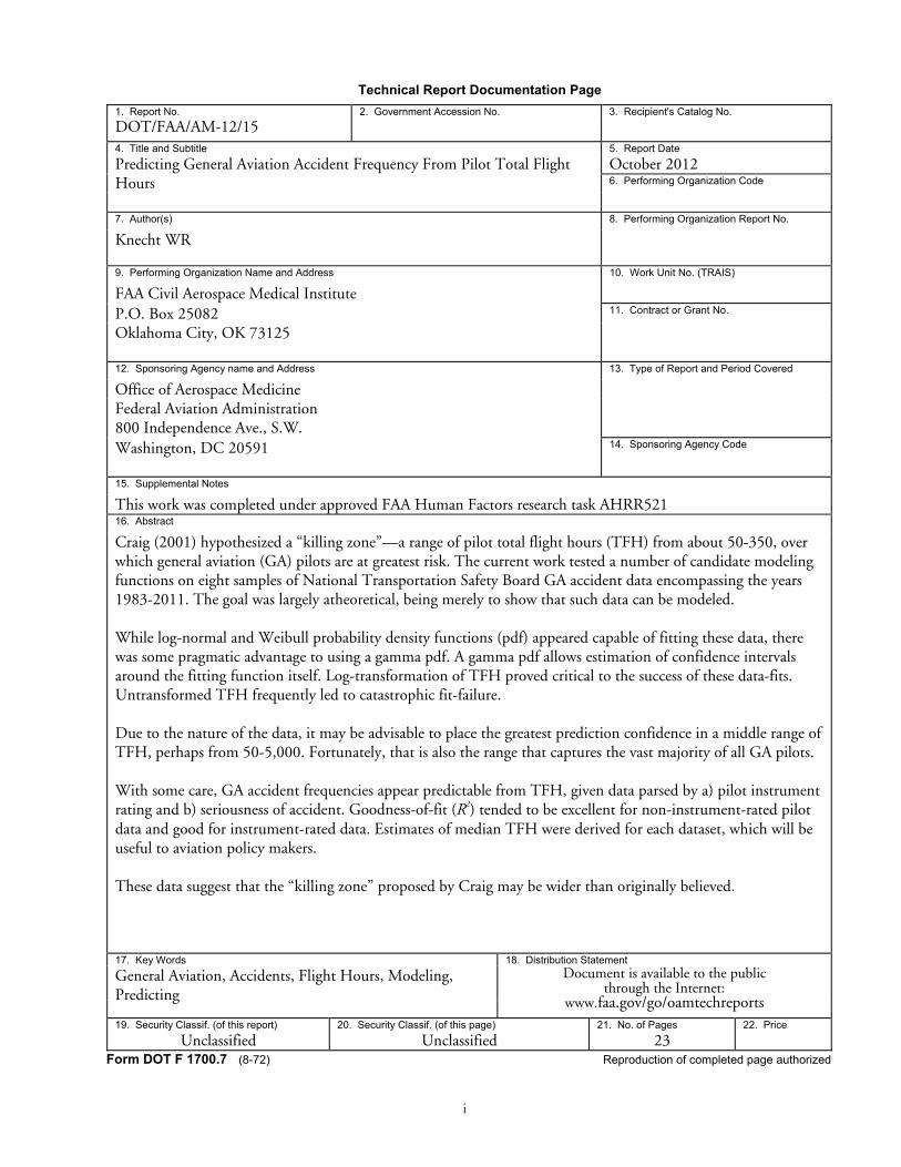
15. Supplemental Notes This work was completed under approved FAA Human Factors research task AHRR521 16. Abstract Craig (2001) hypothesized a “killing zone”—a range of pilot total flight hours (TFH) from about 50-350, over which general aviation (GA) pilots are at greatest risk. The current work tested a number of candidate modeling functions on eight samples of National Transportation Safety Board GA accident data encompassing the years 1983-2011. The goal was largely atheoretical, being merely to show that such data can be modeled. While log-normal and Weibull probability density functions (pdf) appeared capable of fitting these data, there was some pragmatic advantage to using a gamma pdf. A gamma pdf allows estimation of confidence intervals around the fitting function itself. Log-transformation of TFH proved critical to the success of these data-fits. Untransformed TFH frequently led to catastrophic fit-failure. Due to the nature of the data, it may be advisable to place the greatest prediction confidence in a middle range of TFH, perhaps from 50-5,000. Fortunately, that is also the range that captures the vast majority of all GA pilots. With some care, GA accident frequencies appear predictable from TFH, given data parsed by a) pilot instrument rating and b) seriousness of accident. Goodness-of-fit (R2) tended to be excellent for non-instrument-rated pilot data and good for instrument-rated data. Estimates of median TFH were derived for each dataset, which will be useful to aviation policy makers. These data suggest that the “killing zone” proposed by Craig may be wider than originally believed.
17. Key Words 18. Distribution Statement
General Aviation, Accidents, Flight Hours, Modeling, Predicting
Document is available to the public through the Internet:
www.faa.gov/go/oamtechreports 19. Security Classif. (of this report) 20. Security Classif. (of this page) 21. No. of Pages 22. Price
Unclassified Unclassified 23 Form DOT F 1700.7 (8-72) Reproduction of completed page authorized


iii
ACKNOWLEDGMENTS
Deep appreciation is extended to Joe Mooney, FAA (AVP-210), for his help reviewing the NTSB
database queries, which provided the data used here, and to Dana Broach, FAA (AAM-500), for valuable
commentary on this manuscript.


v
CONTENTS
Predicting General Aviation Accident Frequency From Pilot Total Flight Hours
IntroductIon . . . . . . . . . . . . . . . . . . . . . . . . . . . . . . . . . . . . . . . . . . . . . . . . . . . . . . . . . . . . . . . . . . 1
Method . . . . . . . . . . . . . . . . . . . . . . . . . . . . . . . . . . . . . . . . . . . . . . . . . . . . . . . . . . . . . . . . . . . . . . 1
Choosing a modeling function . . . . . . . . . . . . . . . . . . . . . . . . . . . . . . . . . . . . . . . . . . . . . . . . . . . 1
The test data . . . . . . . . . . . . . . . . . . . . . . . . . . . . . . . . . . . . . . . . . . . . . . . . . . . . . . . . . . . . . . . . 3
results . . . . . . . . . . . . . . . . . . . . . . . . . . . . . . . . . . . . . . . . . . . . . . . . . . . . . . . . . . . . . . . . . . . . . . . 4
Goodness of fit . . . . . . . . . . . . . . . . . . . . . . . . . . . . . . . . . . . . . . . . . . . . . . . . . . . . . . . . . . . . . . . 4
Final choice of a fitting function . . . . . . . . . . . . . . . . . . . . . . . . . . . . . . . . . . . . . . . . . . . . . . . . . . 5
Estimating parameter start values for Gpdf
. . . . . . . . . . . . . . . . . . . . . . . . . . . . . . . . . . . . . . . . . . 6
Parameter confidence intervals for Gpdf
. . . . . . . . . . . . . . . . . . . . . . . . . . . . . . . . . . . . . . . . . . . . 6
Using Gpdf
. . . . . . . . . . . . . . . . . . . . . . . . . . . . . . . . . . . . . . . . . . . . . . . . . . . . . . . . . . . . . . . . . . 6
Quantizing Gpdf
. . . . . . . . . . . . . . . . . . . . . . . . . . . . . . . . . . . . . . . . . . . . . . . . . . . . . . . . . . . . . 6
A conservative appraisal of model accuracy at extreme x-values . . . . . . . . . . . . . . . . . . . . . . . . . . 8
dIscussIon. . . . . . . . . . . . . . . . . . . . . . . . . . . . . . . . . . . . . . . . . . . . . . . . . . . . . . . . . . . . . . . . . . . . . . 9
references . . . . . . . . . . . . . . . . . . . . . . . . . . . . . . . . . . . . . . . . . . . . . . . . . . . . . . . . . . . . . . . . . . . 10
AppendIx A: Comparing data fits for the eight datasets of Table 1 . . . . . . . . . . . . . . . . . . . . . . . . . . A1
AppendIx.B: Estimates for the gamma pdf ’s parameters α and β calculated . . . . . . . . . . . . . . . . . . . B1
AppendIx.C: Mathematica code used to generate data for this paper . . . . . . . . . . . . . . . . . . . . . . . . .C1


1
Predicting general aviation accident Frequency From Pilot total Flight hours
1
5000 10 000 15000 20 000 25000
10
20
30
40
50
60
70
6 7 8 9 10
10
20
30
40
50
60
70
a b
INTRODUCTION
Figure 1a shows an example of one category of data we frequently see in general aviation (GA) accident analysis. This is a histogram of fatal accident counts for instrument-rated pilots of GA aircraft1 as a function of pilots’ total flight hours (TFH).2 The data reflect actual U.S. National Transportation Safety Board accident data from 1983-2000, inclusive (NTSB, 2011).
It is not hard to appreciate the usefulness of a modeling function here. Such a function would smooth the noise in the data, allowing investigators to better predict how many pilots of a given experience level are likely to be involved in accidents over a given time period. This would be useful, for instance, in allocating resources for pilot training, or as the basis for a statistical covariate of flight risk. Even a casual glance at Figure 1 shows that policy makers would want to focus on pilots having fewer than 5000 TFH, simply because there are far more accidents in that range. The question is how to get beyond the considerable noise in the data to arrive at more precise estimates of this kind.
1“GA aircraft” are defined here as “all N-tail-numbered aircraft operating in the U.S. under all Federal Aviation Regulations (FAR) Parts except 121 and 135, regardless of airframe type or weight.”2Total flight hours includes all flight time logged at the controls of all aircraft, regardless of aircraft class or category.
METHOD
Choosing a modeling functionIdeally, we like modeling functions to be motivated
by theory about causal processes inherent to our data. However, in the case of aviation risk, we cannot expect these processes to be few or simple.
Three major processes influence the GA accident rate, two of which have their own set of sub-processes.1. Processes that affect the number of pilots at different
values of TFH.a. GA flight is expensive, both in time and money,
plus, it takes time to accumulate flight hours. Hence, we expect that many pilots will have relatively few TFH, with ever-diminishing numbers of pilots as TFH increase.
b. Pilots accumulate TFH at different rates, which may, themselves change, depending on the season of the year, employment situation, the pilot’s economic and social circumstances, and whim.
c. Commercial pilots (those who fly as paid profes-sionals) who also fly GA aircraft have their com-mercial hours included in their TFH. U.S. National Transportation Safety Board (NTSB) data confirm that commercial flying is statistically safer than GA flying.3 So, for these pilots, high TFH does not imply proportionately higher risk.
3Several hundred people are regularly killed each year in GA, a fatal accident rate about 40 times greater than large commercial passenger air carriers such as United, Delta, and American Airlines (source: www.ntsb.gov).
Figure 1. Frequency histogram of a) fatal accident count (y-axis) for instrument-rated GA pilots as a function of total flight hours (x-axis, bin size=100), b) the same data with a natural log-transformed x-axis.

2
d. Pilots constantly enter and leave the pilot popula-tion at independent rates, due to economic factors and/or old age.
e. Pilots leave one data collection category and enter another, when obtaining a new category of pilot license or certification (e.g., getting an instrument rating).
2. Processes that affect each individual pilot’s flight risk. a. Pilots differ in innate, average skill. b. Flight risk tends to be low when pilots are students,
to increase when they first begin to fly solo, then to decrease after they gain experience (Craig, 2001).
c. Some aspects of flight tend to be more danger-ous, for example takeoffs, landings, night flights, and flights in or near severe weather. The type of flight a particular pilot typically engages may differ from another pilot, which will have an affect on the exposure to these more dangerous maneuvers. For example, a pilot who typically makes shorter flights will have more takeoffs and landings per unit time period than a pilot who typically flies longer cross-country flights. Therefore, TFH will never be a perfect proxy for risk.
3. Finally, in some particular data (e.g., those of Figure 1), pilots are included who were passengers having little or nothing to do with the cause of the accident itself.4
Given such complexity, we might despair at trying to model these kinds of data. Then again, as George Box observed “All models are wrong, but some are useful” (Box & Draper, 1987, p. 424). Perhaps we can begin with seeing if any modeling function can fit these data. If so, then we can at least make useful predictions about expected accident rates, even though these may not be purely theoretic.
In the present work, we proceed with this restricted goal, using a standard technique of minimizing least-squares residuals between actual data and a simple model involving just two component functions. The first component will be a simple log-transform. The second will involve that class of particularly useful modeling functions, the probability density functions (pdfs) based on the natural logarithm e. These enclose an area of 1.0 under their curves, making them useful in statistical analysis (Spanier & Oldham, 1987). That class includes the Gaussian (normal), Poisson, log-normal, Weibull, beta, and gamma pdfs.
4Data source: NTSB downloadable aviation accident database www.ntsb.gov/avdata/. Obviously, some readers may object to including pilots who were not directly responsible for the accident. However, bear in mind that we are merely describing an analytical method here, not trying to support specific theoretical statements about accident causation. Moreover, a previous study conducted by the author indicate that about 90% of GA accidents involve single-pilot flights, where there is no dispute over responsibility.
To illustrate such functions, let us single out the gamma pdf (G
pdf). This is a 2-parameter function with a shape pa-
rameter α > 0 and a scale parameter b > 0. Gamma pdfs have been used to model a wide variety of processes, including the size of insurance claims (Hogg & Klugman, 1984), amounts of rainfall (Chiew, Srikanthan, Frost, & Payne, 2005), waiting times and mean-time-to-failure (where it represents time until the αth event in a constant-hazard model), and distributions of microburst wind velocity (Mackey, 1998). Since the GA pilot population arguably consists of a number of sub-populations, some having an accident rate being a function of pilot experience and numbers of pilots—both perhaps inversely related to TFH—Gpdf
is a logical function to test. The basic G
pdf is represented as a function of x (TFH),
α (alpha), and b (beta)
( ) ( )αββα
ααβ
Γ=Γ
−−− 1
,; xexx
pdf (1)
with the gamma function G(α) itself described as the Euler integral of the second kind, defined for α > 0
dtet t
0
1 (2)
Figure 2 shows the behavior of Gpdf
with several differ-ent parameter values. We can easily imagine that such a function could be fitted to our kinds of data.
Given our data, a number of practical issues arise:1. The characteristically long tail of the raw data results
in a very poor fit to any kind of pdf.2. A location (shift) parameter will be required, since
TFH does not start at zero for instrument-rated pilots.3. An amplitude term will be required to scale the unit
pdf, whose area under the curve is 1.0, to the binned data, whose area under the curve is much greater.
4.Gpdf should rightfully be tested alongside other plausible
candidate distributions.5. Once we arrive at a preferred fitting function, methods
should be described regarding:a. Estimation of starting values for constrained pa-
rameter searchb. Goodness of fit with the original datac. Calculation of selected confidence intervalsd. Quantizing the area under the function
Issue 1 suggests a very simple approach, namely, a compressive transform of the x-axis. Indeed, a natural-log compression might prove suitable for “shrinking the tail,” to make the raw data of Figure 1a look more like something found in Figure 2.

3
Issues 2 and 3 are purely practical. A location parameter d(delta) will overcome the problem of non-zero initial data values, while an amplitude term (A) will scale the area under the pdf to our data.
These modifications of Equation 1 lead to the test-able form:
( ) ( )αβδβα
ααβδ
Γ−=Γ
−−−− 1))(ln( ))(ln(,; xeAxx
Issue 4 requires empirical testing of a reasonable set of candidate pdfs (Winkelmann, 2008). Given the nature of the data, we can immediately rule out some candidates.5 For instance, a quick glance at Figure 1a shows that a symmetrical distribution (e.g., Gaussian) obviously cannot fit our data. Additionally, we probably want a function capable of representing overdispersion (variance > mean) or underdispersion (variance < mean). That would rule out the Poisson, where the variance can only equal the mean.
Given these considerations, gamma, log-normal, Weibull, and beta pdfs remain as logical candidates. Because closed solutions do not exist for finding optimal parameter values to such functions, numerical methods must be used. These present their own challenges, as we shall see.
For this study, the NonlinearFit function of Math-ematica 7.0 (Wolfram, 2008) was used for parameter estimation. For un-constrained parameters, NonlinearFit offers a range of standard numerical methods (e.g., Newton-Gauss, quasi-Newton, Levenberg-Marquardt). For constrained parameters, where start-ing and/or final parameter values at time t are forced to lie within some
5During review of this paper, one reviewer asked about the negative binomial function. This was also tested but eliminated due to frequent optimization failure.
range pmin
<pt<p
max, a method such as Karush-Kuhn-Tucker
(KKT) is preferable.An alternative approach might be to use a method like
simulated annealing, guaranteed to find a global mini-mum (Kirkpatrick, Gelatt, Vecchi, 1983; Černý, 1985). However, such methods are computationally intensive and slow, providing little additional benefit, provided we show prudence in our method.
Finally, Issue 5 suggests finding a method for mapping the area under the fitting curve into quantiles, say at 10% intervals. For the time being, let us postpone that discus-sion until after we settle on a single fitting function and gain some experience in seeing how that function behaves.
The test dataFour candidate model classes were tested: beta, gamma,
log-normal, and Weibull pdfs. These were fitted to eight U.S. GA pilot data sets, described in Table 1. The data sets spanned two time periods (1983-2000 and 2001-May 15, 2011), two categories of injury (Serious vs. Fatal),6 and two categories of pilot instrument rating (Instrument-rated vs. Non-instrument-rated). The data consisted of all pilots involved in U.S. GA accidents during the time period speci-fied, regardless of whether the pilot in question appeared to be legally responsible for the accident.
6NTSB classifies a “serious” or “fatal” accident as one where at least one person onboard at least one airplane was seriously or fatally injured, respectively.
2
Figure 2. pdf with various values of and .
3
Table 1. Number of pilots (n) in the ijkth data test set
Time Period (i) 1983-2000 2001-2011
Accident Category (j) SERIOUS FATAL SERIOUS FATAL
Instrument-rated pilots (k) n111= 362 n121= 831 n211=164 n221=465
Non-instrument-rated pilots n112=1051 n122=1823 n212=328 n222=571
(3)

4
The raw data were first aggregated into histograms with x-axis bins 100 TFH wide. To aid visual inspection, Appendix A shows one row of data fits using Eq. 3 and a second row using Eq. 1, where the log transform was performed prior to the data fit. The latter is included because that particular method makes it much easier to visualize the underlying functional fit differences.
RESULTS
Goodness of fitAs expected, both the log-transform of TFH and the
inclusion of the location parameter d proved essential. Without the log-transform, parameter estimates failed to converge for nearly all datasets. And, without d, the same held true for instrument-rated pilot datasets.
Even with the log-transform and d, however, beta functions rarely produced good data fits. Therefore, beta was eliminated from further consideration as a modeling function, and for the sake of parsimony, results are not shown here. The three remaining fitting functions and eight datasets produced 24 models. Appendix A shows these, with model performance and parameter estimates.
Model goodness-of-fit can be expressed by a variety of metrics. One of the simplest is the coefficient of determi-nation R2, which varies between 0 and 1, and estimates the proportion of explained variance.
( )( )∑
∑=
=
−
−−=−= n
i x
n
i xx
total
error
yy
fySSSSR
12
12
2 11
Here, fx represents the predicted value of y at x, versus
the observed value of yx. Lower R2s merely reflect noisier
data, not necessarily fitting failure.Two aspects of the data affected both the size of R2 and
the stability of model parameter estimates, as measured by the breadth of their confidence intervals. As expected, greater random variation (noise) in the data and smaller sample size (n
pilots) both led to lower R2s. Binning the
data, of course, helps dampen noise, but at the expense of lowering the effective sample size, which becomes the number of bins (n
bins) rather than n
pilots. Figure 3 shows
that better results tended to occur with models based
on npilots
> 300, while little additional advantage resulted from n
pilots > 1000.
Confidence intervals for the underlying correlation r=Sqrt(R2) can be estimated using Fisher’s method (Glass & Hopkins, 1984, pp. 304-307).
31
1ln5.0tanhtanh
nz
rr
rzZr CIzCI
where Z is Fisher’s Z-transform of r, sz (sigma sub-z) is
the standard error of Z, and zCI
is the normal z–value corresponding to the desired confidence interval (e.g., for .95CI, z
CI =1.96).
Based on R2, the gamma, log-normal, and Weibull pdfs all appeared reasonable candidates for use with this broad range of accident categories. Appendix A shows R2s ranging from .862-.994, considered good-to-excellent.
While it was possible to get Poisson models to converge, the R2s were uniformly and significantly lower than, for instance, those of Gamma (p
Wilcoxon=.012), supporting
exclusion of the Poisson from further consideration. Table 2 compares the two.
The three remaining model classes can be statisti-cally compared by setting up R2s as if each of the eight datasets were an “individual,” and the three models were repeated measures experienced by each “individual.” The three “Raw data” rows in Table 3 show the setup of this comparison.
4
500 1000 1500npilots
0.88
0.90
0.92
0.94
0.96
0.98
1.00
R2
Figure 3. Plot of npilots (x-axis) versus resulting R2 (y-axis), with least-squares trend line.
5
Table 2. Comparing Poisson and Gamma R2s
Dataset 1 2 3 4 5 6 7 8 Mean Median Gamma .994 .940 .994 .932 .983 .946 .967 .864 .953 .957 Poisson .890 .770 .880 .748 .929 .873 .892 .840 .853 .877
(5)
Figure 3. Plot of npilots (x-axis) versus resulting R2 (y-axis), with least-squares trend line.
(4)

5
6
Table 3. Comparing Gamma, Log-normal, and Weibull R2s
Dataset 1 2 3 4 5 6 7 8 Mean Median
Gamma 0.994 0.940 0.994 0.932 0.983 0.946 0.967 0.864 0.953 0.957
Log-normal 0.994 0.942 0.994 0.931 0.982 0.947 0.964 0.862 0.952 0.956Raw data
Weibull 0.993 0.923 0.994 0.931 0.982 0.948 0.968 0.872 0.951 0.958
Gamma 2.903 1.738 2.903 1.673 2.380 1.792 2.044 1.309 2.093 1.918
Log-normal 2.903 1.756 2.903 1.666 2.351 1.802 2.000 1.301 2.085 1.901Z-transformed
Weibull 2.826 1.609 2.903 1.666 2.351 1.812 2.060 1.341 2.071 1.936
Quick inspection of these raw R2s shows no prominent differences between modeling functions. Analysis of variance (ANOVA) can confirm that. But, first we have to consider that our theoretical distributions of of R2 are not expected to be normal, since R2 is range-restricted to 0<R2<1.0. ANOVA is famously tolerant of some devia-tion from normality, but these R2s are high, and might be a problem. Indeed, Monte Carlo simulation reveals considerable negative skewness, as Figure 4a illustrates.
We can correct that skewness using Fisher’s Z- transform, a variant of Equation 5:
−
+= 2
22
1
1ln5.0
R
RRcorrected
Figure 4b illustrates the resulting improvement in normality. Applying that method to all our R2s produces the bottom, “Z-transformed” half of Table 3, which we can now more legitimately analyze.
Subsequent ANOVA reveals no significant differences between the gamma, log-normal, and Weibull R2s (p =.429, NS, Greenhouse-Geisser-corrected for non-sphericity).
One salient feature distinguishing the three model classes was the left-hand side of the curve. As Appendix A makes plain in ln(x)-space, Weibull pdfs tended to be “fatter” on the left, whereas gamma and log-normal pdfs tended to be more symmetrical and to resemble each other more closely. The exact nature of the leftmost, lowest-TFH end of these distributions is something that can be investigated more closely in future years, as data accumulate, allowing more reliable statistical analysis.
Final choice of a fitting functionJudging solely by R2 and x̃pdf, it would be imprudent
to recommend one model over another on the grounds of theory. Arguably, though, the gamma pdf G
pdf is most useful
for two reasons. To a lesser extent, experience with these data showed that G
pdf was the easiest function to fit. More
compellingly, Gpdf
allows calculation of confidence bands around the modeling function itself. These confidence bands provide estimates of the net stability of predictions based on each dataset. Appendix A shows how these confidence bands are influenced by dataset size n
ijk, as intimated earlier
by Figure 3. Smaller datasets are considerably less reliable.For these pragmatic reasons, we choose to examine
Gpdf
in detail for the rest of this report.
7
a b (skew = -0.815) (skew = -0.021)
Figure 4. a) Frequency histograms for 1000 Monte Carlo-simulated R2s randomly generated by one of our Gpdf models. The y-axis shows the frequency count of R2s in each x-axis bin. Note the negative skew; b) Z-transform corrects this negative skew.
(6)
6
Estimating parameter start values for Gpdf
The raw data show considerable noise. This produces lumpy parameter residual error spaces and the risk of optimization failure due to local minima. Numerical methods for G
pdf parameter estimates therefore benefit
from having start values as close as possible to final values.Estimates for α and b can be derived by the method
of moments (see Appendix B for details).
( )( )2
112
2
1
∑∑∑
==
=
−=
n
i in
i i
n
i iest
xxn
xα
( )∑
∑∑=
==−
= n
i i
n
i in
i iest
x
nxx
1
2
112
β
A start value for the amplitude term (A) can be esti-mated as
( )( )
( )αββα ααβ
Γ−
== −−− 11xmax
Mo,
max,est e
yyy
A
where, of the binned data, ymax
is the maximum function height, and y
Mo is the height of the model G
pdf mode7(M
o) of
( )βα 10 −=M (10)
Finally, we can estimate the location parameter (d) by forcing the peaks of both the data and G
pdf to take the
same x-value. This leads to
(11)
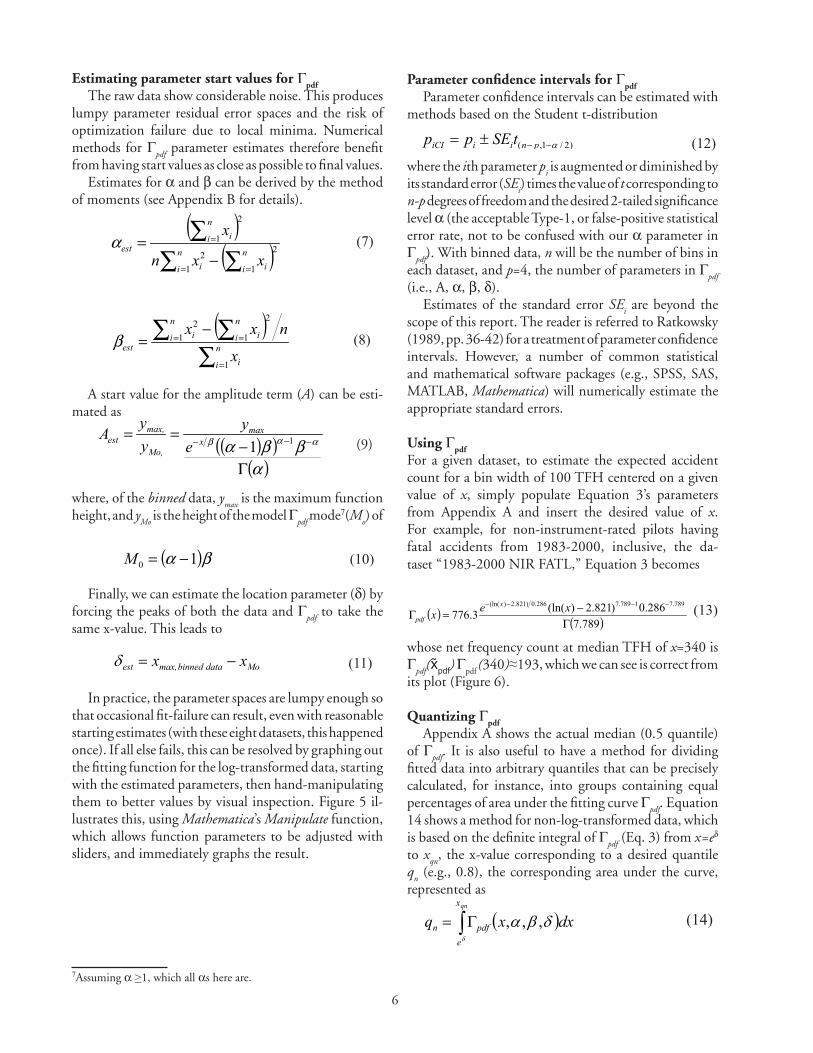
In practice, the parameter spaces are lumpy enough so that occasional fit-failure can result, even with reasonable starting estimates (with these eight datasets, this happened once). If all else fails, this can be resolved by graphing out the fitting function for the log-transformed data, starting with the estimated parameters, then hand-manipulating them to better values by visual inspection. Figure 5 il-lustrates this, using Mathematica’s Manipulate function, which allows function parameters to be adjusted with sliders, and immediately graphs the result.
7Assuming α >1, which all αs here are.
Parameter confidence intervals for Gpdf
Parameter confidence intervals can be estimated with methods based on the Student t-distribution
(12)where the ith parameter p
i is augmented or diminished by
its standard error (SEi) times the value of t corresponding to
n-p degrees of freedom and the desired 2-tailed significance level α (the acceptable Type-1, or false-positive statistical error rate, not to be confused with our α parameter in G
pdf). With binned data, n will be the number of bins in
each dataset, and p=4, the number of parameters in Gpdf
(i.e., A, α, b, d).
Estimates of the standard error SEi are beyond the
scope of this report. The reader is referred to Ratkowsky (1989, pp. 36-42) for a treatment of parameter confidence intervals. However, a number of common statistical and mathematical software packages (e.g., SPSS, SAS, MATLAB, Mathematica) will numerically estimate the appropriate standard errors.
Using Gpdf
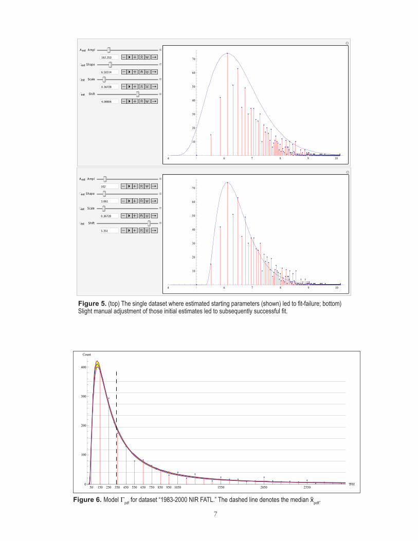
For a given dataset, to estimate the expected accident count for a bin width of 100 TFH centered on a given value of x, simply populate Equation 3’s parameters from Appendix A and insert the desired value of x. For example, for non-instrument-rated pilots having fatal accidents from 1983-2000, inclusive, the da-taset “1983-2000 NIR FATL,” Equation 3 becomes
( ) ( )789.7286.0)821.2)(ln(3.776
789.71789.7286.0)821.2)(ln(
Γ−=Γ
−−−− xexx
whose net frequency count at median TFH of x=340 is G
pdf(xp̃df)Gpdf
(340)≈193, which we can see is correct from its plot (Figure 6).
Quantizing Gpdf
Appendix A shows the actual median (0.5 quantile) of G
pdf. It is also useful to have a method for dividing
fitted data into arbitrary quantiles that can be precisely calculated, for instance, into groups containing equal percentages of area under the fitting curve G
pdf. Equation
14 shows a method for non-log-transformed data, which is based on the definite integral of G
pdf (Eq. 3) from x=ed
to xqn
, the x-value corresponding to a desired quantile q
n (e.g., 0.8), the corresponding area under the curve,
represented as
(14)
(7)
(8)
(9)
Modatabinnedmax,est xx
1
)2/1,( α−−±= pniiiCI tSEpp
1
( )∫Γ=qnx
epdfn dxxq
δ
δβα ,,,
(13)
7
9
50 150 250 350 450 550 650 750 850 950 1050 1550 2050 2550TFH0
100
200
300
400
Count
Figure 6. Model pdf for dataset “1983-2000 NIR FATL.” The dashed line denotes the median xp̃df.
Figure 6. Model Gpdf for dataset “1983-2000 NIR FATL.” The dashed line denotes the median x̃pdf.8
A est Ampl
162.253
�est Shape
6.50314
�est Scale
0.36728
�est Shift
4.08806
4 6 7 8 9 10
10
20
30
40
50
60
70
A est Ampl
102
�est Shape
3.061
�est Scale
0.36728
�est Shift
5.351
4 6 7 8 9 10
10
20
30
40
50
60
70
Figure 5. top) The single dataset where estimated starting parameters (shown) led to fit-failure; bottom) Slight manual adjustment of those initial estimates led to subsequently successful fit.
Figure 5. (top) The single dataset where estimated starting parameters (shown) led to fit-failure; bottom) Slight manual adjustment of those initial estimates led to subsequently successful fit.

8
There is no closed-form solution for arbitrary xqn
. Fortunately, an iterative numerical method is easily stated. We note that the minimum value of G
pdf = 0
in the linear domain is specified by x=ed, and that we normalize the area under G
pdf, given that it computa-
tionally represents n pilots put into bins 100 FH wide.
1
cnpilots
x
epdfqn qndxx εε
δ
<−
Γ=→ ∫ 100
In other words, start with an arbitrary value for x,
integrate Gpdf
(Eq. 3) to find the area under the curve from ed to x, next calculate the error e between that area and our desired quantile, and then adjust x in the direction that minimizes e, halting when e falls below a critical tolerance value e
c (epsilon sub-c). This is easily
done with software such as Mathematica, given a simple statement such as
FindArgMin[Abs[(NIntegrate[Gpdf[x],{x,Ed,mu}]/(100*n))-qn],{mu,Quantile[data,qn] }][[1]];8
The data of Figure 6 produce the plot for e:
Naturally, the minimization algorithm will oscillate around the discontinuity, but this poses no practical problem to finding an accurate solution for the median.
A conservative appraisal of model accuracy at ex-treme x-values
Extensive experience with “extreme” datasets, such as the ones encountered here, teaches us to be wary of what otherwise may seem like high-precision modeling at very
8Here, Quantile[data,qn] is just a specification to the function FindArgMin, telling it to find the minimum of |(Gpdf(x)/100n)-qn|, starting at x-value mu, specified as the desired quantile of the raw data, which Mathematica conveniently has a built-in function to find.
low and very high values of x (here being TFH). Often, we find that conservative interpretation works best. In other words, we consciously choose to limit high “logical confidence” in predicted accident frequency to a middle range of, say, 50-5,000 TFH.
The roots of this conservativism are grounded in model construction, sampling, and residual error spaces. Residual error is, of course, the average squared difference between the ys our model predicts, given the x-values of the data. Total residual error is the quantity we wish to minimize by adjusting our model parameters. Now, what we some-times see is that this residual error can be minimized pretty well by a range of models, all of which provide a pretty good fit to most of the data. This happens when we have a complex residual error landscape with many local hills and valleys (as opposed to a simple, monotonic landscape with just one deep, global minimum).
The exact geometry of the error space is, of course, largely dictated by the data. But, it is also a function of the model and of how the data are set up. For instance, suppose we have two accidents, one at 15,000 TFH, the other at 15,050 TFH. In that event, the error space very much depends how wide our sampling bins are and
where each bin starts and finishes on x. In the very long right-hand tail of data like ours, the typical actual ac-cident frequency bin count is going to be 0. But, if our bins are wide along x, or spaced in a certain way on the x-axis, instead of getting two bins, each 1 unit high, we can end up with one bin 2 units high. Amidst a sea of bins 0 units high, the residual error of this 2-accident bin will be almost (2-0)2 = 4, as opposed to the 2(1-0)2 = 2 units it would otherwise be.
The point is that the right-hand tail of distributions like these can become “logically unreliable.” Most bins in the long right-hand tail will contain zero cases. Con-sequently, the farther out on the x-axis a non-zero bin is,
10
xqn
Figure 7. Plot of Eq. 15 for “1983-2000 NIR FATL,” here minimizing at the median xqn = xp̃df.
Figure 7. Plot of Eq. 15 for “1983-2000 NIR FATL,” here minimizing at the median xqn = xp̃df.
(15)
9
the greater its effect on model parameters. That makes the far end of a long-tailed distribution less trustworthy than we would like it to be.
The left-hand end of this kind of distribution is also somewhat troubled, as we can see from the confidence intervals in Appendix A. Many of these confidence in-tervals tend to be wide on the left, which also happens to be a region of relatively few accidents. The very lowest TFH bin is often not far removed from the very tallest, in which case a small d shift in the curve to the right or left, can accompany a large change in the amplitude parameter A, and/or a large shift in α and/or b. All this goes to show that highly sloped frequency distributions can sometimes be represented by a multiplicity of pretty good models which, nonetheless, may vary widely in pa-rameter estimates, which differ most in their predictions at extreme values of x.
Therefore, as stated previously, we are prudent to put our greatest faith in the middle TFH ranges for these models, perhaps in the 50-5,000 TFH range. Fortunately, that is the range most interesting to most of us under most circumstances, because it captures the vast majority of accidents.
DISCUSSION
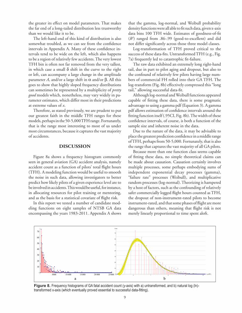
Figure 8a shows a frequency histogram commonly seen in general aviation (GA) accident analysis, namely accident count as a function of pilots’ total flight hours (TFH). A modeling function would be useful to smooth the noise in such data, allowing investigators to better predict how likely pilots of a given experience level are to be involved in accidents. This would be useful, for instance, in allocating resources for pilot training or mentoring, and as the basis for a statistical covariate of flight risk.
In this report we tested a number of candidate mod-eling functions on eight samples of NTSB GA data encompassing the years 1983-2011. Appendix A shows
11
5000 10 000 15000 20 000 25000
10
20
30
40
50
60
70
6 7 8 9 10Log�TFH �0
10
20
30
40
50
60
70
Count
a b
Figure 8. Frequency histograms of GA fatal accident count (y-axis) with a) untransformed, and b) natural log (ln)-transformed x-axis (which eventually proved essential to successful data-fitting).
that the gamma, log-normal, and Weibull probability density functions were all able to fit such data, given x-axis data bins 100 TFH wide. Estimates of goodness-of-fit (R2) ranged from .86-.99 (good-to-excellent) and did not differ significantly across those three model classes.
Log-transformation of TFH proved critical to the success of these data-fits. Untransformed TFH (e.g., Fig. 7a) frequently led to catastrophic fit-failure.
The raw data exhibited an extremely long right-hand tail, due in part to pilot aging and dropout, but also to the confound of relatively few pilots having large num-bers of commercial FH rolled into their GA TFH. The log-transform (Fig. 8b) effectively compressed this “long tail,” allowing successful data-fit.
Although log-normal and Weibull functions appeared capable of fitting these data, there is some pragmatic advantage to using a gamma pdf (Equation 3). A gamma pdf allows estimation of confidence intervals around the fitting function itself (.95CI, Fig. 8b). The width of these confidence intervals, of course, is both a function of the sample size and inherent noise in the data.
Due to the nature of the data, it may be advisable to place the greatest prediction confidence in a middle range of TFH, perhaps from 50-5,000. Fortunately, that is also the range that captures the vast majority of all GA pilots.
Because more than one function class seems capable of fitting these data, no simple theoretical claims can be made about causation. Causation certainly involves multiple processes, some perhaps embodying sums of independent exponential decay processes (gamma), “failure rate” processes (Weibull), and multiplicative random processes (log-normal). Theorizing is hampered by a host of factors, such as the confounding of relatively safer commercially logged flight hours counted as TFH, the dropout of non-instrument-rated pilots to become instrument-rated, and that some phases of flight are more dangerous than others, meaning that flight risk is not merely linearly proportional to time spent aloft.
10
Therefore, the goal of the current effort is largely atheoretical, being merely to show that such data can be modeled. With some care, GA accident frequencies can be predicted from TFH, given data parsed by a) pilot instru-ment rating and b) seriousness of accident. Goodness-of-fit (R2) tended to be excellent for non-instrument-rated pilot data and good for instrument-rated data. Estimates of median TFH were derived for each dataset, which will be useful to aviation policy makers.
REFERENCES
Box, G.E.P., & Draper, N.R. (1987). Empirical model-building and response surfaces, New York: Wiley.
Černý, V. (1985). Thermodynamical approach to the traveling salesman problem: An efficient simula-tion algorithm. Journal of Optimization Theory and Applications, 45: 41–51.
Chiew, F.H.S., Srikanthan, R., Frost, A.J., & Payne, E.G.I. (2005). Reliability of daily and annual stochastic rainfall data generated from different data lengths and data characteristics. In: MODSIM 2005 In-ternational Congress on Modelling and Simulation, Modelling and Simulation Society of Australia and New Zealand, Melbourne, December 2005, pp. 1223-1229.
Craig, P.A. (2001). The killing zone. New York: McGraw-Hill.
Glass, G.V., & Hopkins, K.D. (1984). Statistical methods in education and psychology. Englewood Cliffs, NJ: Prentice-Hall.
Hogg, R.V., & Klugman, S.A. (1984). Loss distributions. New York: Wiley.
Kirkpatrick, S., Gelatt, C.D., & Vecchi, M.P. (1983). Optimization by simulated annealing. Science 220 (4598): 671-80.
Mackey, J.B. (1998). Forecasting wet microbursts associ-ated with summertime airmass thunderstorms over the southeastern United States. Unpublished MS Thesis, Air Force Institute of Technology.
National Transportation Safety Board. (2011). User-downloadable database. Downloaded May 26, 2011, from www.ntsb.gov/avdata
Ratkowsky, D.A. (1989). Handbook of nonlinear regression models. New York: Marcel Dekker.
Spanier, J. & Oldham, K.B. (1987). An atlas of functions. New York: Hemisphere.
Winkelmann, R. (2008). Econometric analysis of count data. (5th Ed.). Berlin: Springer-Verlag.
Wolfram Mathematica Documentation Center. Some notes on internal implementation. Downloaded April 29, 2011, from http://reference.wolfram.com/mathematica/note/SomeNotesOnInternalImple-mentation.html#20880
A1
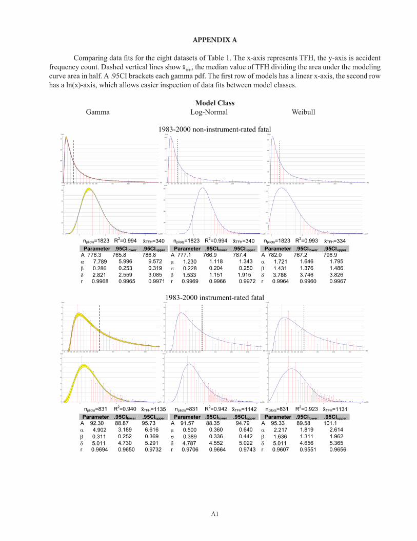
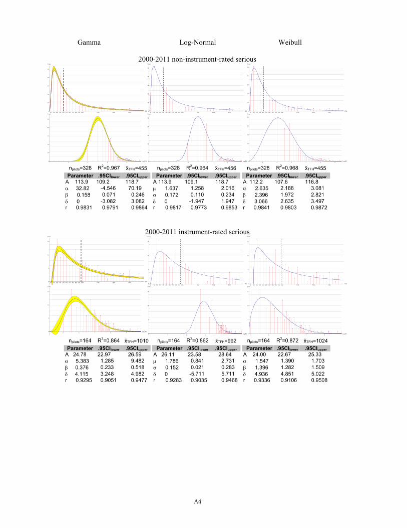
APPENDIX A
Comparing data fits for the eight datasets of Table 1. The x-axis represents TFH, the y-axis is accident frequency count. Dashed vertical lines show x̃TFH, the median value of TFH dividing the area under the modeling curve area in half. A .95CI brackets each gamma pdf. The first row of models has a linear x-axis, the second row has a ln(x)-axis, which allows easier inspection of data fits between model classes.
Model Class Gamma Log-Normal Weibull
12
1983-2000 non-instrument-rated fatal
50 150 250 350 450 550 650 750 850 950 1050 1550 2050 2550TFH0
100
200
300
400
Count
50 150 250 350 450 550 650 750 850 950 1050 1550 2050 2550TFH0
100
200
300
400
Count
50 150 250 350 450 550 650 750 850 950 1050 1550 2050 2550TFH0
100
200
300
400
Count
3 4 5 6 7 8 9Log�TFH �0
100
200
300
400
Count
2 4 6 8Log�FH�0
100
200
300
400
Count
4 5 6 7 8 9Log�FH�0
100
200
300
400
Count
npilots=1823 R2=0.994 xT̃FH=340 npilots=1823 R2=0.994 x̃TFH=340 npilots=1823 R2=0.993 xT̃FH=334 Parameter .95CIlower .95CIupper Parameter .95CIlower .95CIupper Parameter .95CIlower .95CIupperA 776.3 765.8 786.8 A 777.1 766.9 787.4 A 782.0 767.2 796.9 7.789 5.996 9.572 1.230 1.118 1.343 1.721 1.646 1.795 0.286 0.253 0.319 0.228 0.204 0.250 1.431 1.376 1.486 2.821 2.559 3.085 1.533 1.151 1.915 3.786 3.746 3.826 r 0.9968 0.9965 0.9971
r 0.9969 0.9966 0.9972 r 0.9964 0.9960 0.9967
1983-2000 instrument-rated fatal
50 150 250 350 450 550 650 750 850 950 1050 1550 2050 2550TFH0
10
20
30
40
50
60
70
Count
50 150 250 350 450 550 650 750 850 950 1050 1550 2050 2550TFH0
10
20
30
40
50
60
70
Count
50 150 250 350 450 550 650 750 850 950 1050 1550 2050 2550TFH0
10
20
30
40
50
60
70
Count
6 7 8 9 10Log�TFH �0
10
20
30
40
50
60
70
Count
5 6 7 8 9 10Log�FH�0
10
20
30
40
50
60
70
Count
6 7 8 9 10Log�TFH �0
10
20
30
40
50
60
70
Count
npilots=831 R2=0.940 xT̃FH=1135 npilots=831 R2=0.942 x̃TFH=1142 npilots=831 R2=0.923 xT̃FH=1131Parameter .95CIlower .95CIupper Parameter .95CIlower .95CIupper Parameter .95CIlower .95CIupper
A 92.30 88.87 95.73 A 91.57 88.35 94.79 A 95.33 89.58 101.1 4.902 3.189 6.616 0.500 0.360 0.640 2.217 1.819 2.614 0.311 0.252 0.369 0.389 0.336 0.442 1.636 1.311 1.962 5.011 4.730 5.291 4.787 4.552 5.022 5.011 4.656 5.365 r 0.9694 0.9650 0.9732
r 0.9706 0.9664 0.9743 r 0.9607 0.9551 0.9656

A2 13
Gamma Log-Normal Weibull
1983-2000 non-instrument-rated serious
50 150 250 350 450 550 650 750 850 950 1050 1550 2050 2550TFH0
50
100
150
200
250
Count
50 150 250 350 450 550 650 750 850 950 1050 1550 2050 2550TFH0
50
100
150
200
250
Count
50 150 250 350 450 550 650 750 850 950 1050 1550 2050 2550TFH0
50
100
150
200
250
Count
3 4 5 6 7 8 9Log�TFH �0
50
100
150
200
250
Count
2 4 6 8Log�FH�0
50
100
150
200
250
Count
4 5 6 7 8 9Log�FH�0
50
100
150
200
250
Count
npilots=1051 R2=0.994 xT̃FH=312 npilots=1051 R2=0.994 xT̃FH=313 npilots=1051 R2=0.994 xT̃FH=307 Parameter .95CIlower .95CIupper Parameter .95CIlower .95CIupper Parameter .95CIlower .95CIupper
A 472.4 465.5 479.2 A 472.4 465.6 479.2 A 475.8 466.6 485.0 8.322 6.163 10.48 1.266 1.133 1.398 1.746 1.667 1.825 0.271 0.236 0.306 0.216 0.189 0.243 1.418 1.361 1.475 2.776 2.476 3.077 1.396 0.930 1.861 3.780 3.738 3.822 rA 0.9968 0.9964 0.9972
rA 0.9968 0.9964 0.9972 rA 0.9968 0.9964 0.9972AThe equality of values for r=0.9968 across distributions here is simply a coincidence.
1983-2000 instrument-rated serious
50 150 250 350 450 550 650 750 850 950 1050 1550 2050 2550TFH0
5
10
15
20
25
30
Count
50 150 250 350 450 550 650 750 850 950 1050 1550 2050 2550TFH0
5
10
15
20
25
30
Count
50 150 250 350 450 550 650 750 850 950 1050 1550 2050 2550TFH0
5
10
15
20
25
30
Count
5 6 7 8 9Log�TFH �0
5
10
15
20
25
30
Count
4 5 6 7 8 9Log�FH�0
5
10
15
20
25
30
Count
6 7 8 9Log�FH�0
5
10
15
20
25
30
Count
npilots=362 R2=0.932 xT̃FH=1067 npilots=362 R2=0.931 xT̃FH=1063 npilots=362 R2=0.931 xT̃FH=1064Parameter .95CIlower .95CIupper Parameter .95CIlower .95CIupper Parameter .95CIlower .95CIupper
A 42.12 39.85 44.38 A 42.36 40.07 44.65 A 42.35 39.61 45.09 10.33 2.150 18.51 1.226 0.765 1.687 2.397 1.878 2.916 0.208 0.126 0.289 0.193 0.109 0.277 1.644 1.260 2.028 4.357 3.449 5.266 3.023 1.434 4.611 5.011 4.600 5.421 r 0.9653 0.9575 0.9717
r 0.9651 0.9572 0.9715 r 0.9650 0.9571 0.9715

A3
14
Gamma Log-Normal Weibull
2000-2011 non-instrument-rated fatal
50 150 250 350 450 550 650 750 850 950 1050 1550 2050 2550TFH0
20
40
60
80
100
Count
50 150 250 350 450 550 650 750 850 950 1050 1550 2050 2550TFH0
20
40
60
80
100
Count
50 150 250 350 450 550 650 750 850 950 1050 1550 2050 2550TFH0
20
40
60
80
100Count
2 4 6 8Log�TFH �0
20
40
60
80
100
Count
2 4 6 8Log�FH�0
20
40
60
80
100
Count
4 5 6 7 8 9Log�FH�0
20
40
60
80
100Count
npilots=571 R2=0.983 xT̃FH=421 npilots=571 R2=0.982 xT̃FH=421 npilots=571 R2=0.982 xT̃FH=424 Parameter .95CIlower .95CIupper Parameter .95CIlower .95CIupper Parameter .95CIlower .95CIupper
A 219.7 213.5 226.0 A 219.7 213.5 225.9 A 231.2 207.5 218.9 17.94 5.006 30.87 1.611 1.305 1.916 2.083 1.855 2.309 0.216 0.141 0.290 0.179 0.128 0.230 1.921 1.704 2.138 1.203 0 2.695 0 -1.534 1.534 3.422 3.207 3.636 r 0.9914 0.9899 0.9927
r 0.9912 0.9896 0.9925 r 0.9912 0.9896 0.9925
2000-2011 instrument-rated fatal
50 150 250 350 450 550 650 750 850 950 1050 1550 2050 2550TFH0
5
10
15
20
25
30
Count
50 150 250 350 450 550 650 750 850 950 1050 1550 2050 2550TFH0
5
10
15
20
25
30
Count
50 150 250 350 450 550 650 750 850 950 1050 1550 2050 2550TFH0
5
10
15
20
25
30
Count
4 5 6 7 8 9 10Log�TFH �0
5
10
15
20
25
30
Count
2 4 6 8 10Log�FH�0
5
10
15
20
25
30
Count
5 6 7 8 9 10Log�FH�0
5
10
15
20
25
30
Count
npilots=465 R2=0.946 xT̃FH=1241 npilots=465 R2=0.947 xT̃FH=1212 npilots=465 R2=0.948 xT̃FH=1218Parameter .95CIlower .95CIupper Parameter .95CIlower .95CIupper Parameter .95CIlower .95CIupper
A 54.03 51.70 56.37 A 55.87 53.41 58.34 A 55.15 52.87 57.43 14.27 4.592 23.96 1.840 1.351 2.330 2.380 2.099 2.660 0.218 0.146 0.289 0.132 0.071 0.193 2.027 1.775 2.279 3.288 2.148 4.429 0 -3.104 3.105 4.568 4.303 4.833 r 0.9726 0.9672 0.9771
r 0.9732 0.9679 0.9776 r 0.9736 0.9684 0.9779
A4
15
Gamma Log-Normal Weibull
2000-2011 non-instrument-rated serious
50 150 250 350 450 550 650 750 850 950 1050 1550 2050 2550TFH0
10
20
30
40
50
Count
50 150 250 350 450 550 650 750 850 950 1050 1550 2050 2550TFH0
10
20
30
40
50
Count
50 150 250 350 450 550 650 750 850 950 1050 1550 2050 2550TFH0
10
20
30
40
50
Count
2 4 6 8Log�TFH �0
10
20
30
40
50
Count
2 4 6 8Log�FH�0
10
20
30
40
50
Count
4 5 6 7 8 9Log�FH�0
10
20
30
40
50
Count
npilots=328 R2=0.967 xT̃FH=455 npilots=328 R2=0.964 xT̃FH=456 npilots=328 R2=0.968 xT̃FH=455 Parameter .95CIlower .95CIupper Parameter .95CIlower .95CIupper Parameter .95CIlower .95CIupper
A 113.9 109.2 118.7 A 113.9 109.1 118.7 A 112.2 107.6 116.8 32.82 -4.546 70.19 1.637 1.258 2.016 2.635 2.188 3.081 0.158 0.071 0.246 0.172 0.110 0.234 2.396 1.972 2.821 0 -3.082 3.082 0 -1.947 1.947 3.066 2.635 3.497 r 0.9831 0.9791 0.9864
r 0.9817 0.9773 0.9853 r 0.9841 0.9803 0.9872
2000-2011 instrument-rated serious
50 150 250 350 450 550 650 750 850 950 1050 1550 2050 2550TFH0
5
10
15
Count
50 150 250 350 450 550 650 750 850 950 1050 1550 2050 2550TFH0
5
10
15
Count
50 150 250 350 450 550 650 750 850 950 1050 1550 2050 2550TFH0
5
10
15
Count
5 6 7 8 9Log�TFH �0
5
10
15
Count
2 4 6 8Log�FH�0
5
10
15
Count
5 6 7 8 9Log�FH�0
5
10
15
Count
npilots=164 R2=0.864 xT̃FH=1010 npilots=164 R2=0.862 xT̃FH=992 npilots=164 R2=0.872 xT̃FH=1024Parameter .95CIlower .95CIupper Parameter .95CIlower .95CIupper Parameter .95CIlower .95CIupper
A 24.78 22.97 26.59 A 26.11 23.58 28.64 A 24.00 22.67 25.33 5.383 1.285 9.482 1.786 0.841 2.731 1.547 1.390 1.703 0.376 0.233 0.518 0.152 0.021 0.283 1.396 1.282 1.509 4.115 3.248 4.982 0 -5.711 5.711 4.936 4.851 5.022 r 0.9295 0.9051 0.9477
r 0.9283 0.9035 0.9468 r 0.9336 0.9106 0.9508
B1
1
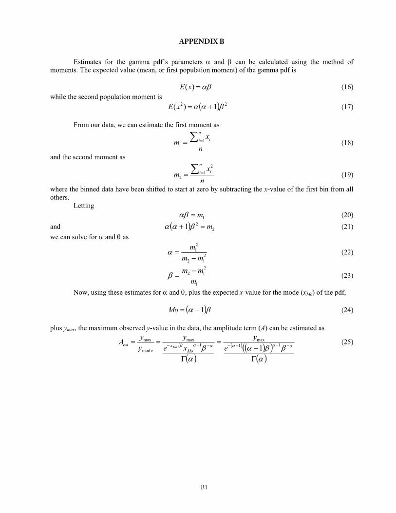
APPENDIX B
Estimates for the gamma pdf’s parameters and can be calculated using the method of moments. The expected value (mean, or first population moment) of the gamma pdf is
)(xE (16) while the second population moment is
22 1)( xE (17)
From our data, we can estimate the first moment as
nx
mn
i i 11 (18)
and the second moment as
nx
mn
i i 12
2 (19)
where the binned data have been shifted to start at zero by subtracting the x-value of the first bin from all others. Letting
1m (20) and 2
21 m (21) we can solve for and as
212
21
mmm
(22)
1
212
mmm
(23)
Now, using these estimates for and , plus the expected x-value for the mode (xMo) of the pdf,
1Mo (24)
plus ymax, the maximum observed y-value in the data, the amplitude term (A) can be estimated as
11
max1
max
mod
max
1ey
xey
yyA
Mox
eest Mo
(25)


C1
16
APPENDIX C

C2
17

C3
18

Related Documents