Predicting Extreme Daily Regime Shifts in Financial Time ...

International Journal of

Financial Studies

Article

Predicting Extreme Daily Regime Shifts in Financial TimeSeries Exchange/Johannesburg Stock Exchange—AllShare Index

Katleho Makatjane * and Ntebogang Moroke

Citation: Makatjane, Katleho, and

Ntebogang Moroke. 2021. Predicting

Extreme Daily Regime Shifts in

Financial Time Series

Exchange/Johannesburg Stock

Exchange—All Share Index.

International Journal of Financial

Studies 9: 18. https://doi.org/

10.3390/ijfs9020018

Academic Editors: Tihana Škrinjaric

and Indranil SenGupta

Received: 4 January 2021

Accepted: 16 March 2021

Published: 25 March 2021

Publisher’s Note: MDPI stays neutral

with regard to jurisdictional claims in

published maps and institutional affil-

iations.

Copyright: © 2021 by the authors.

Licensee MDPI, Basel, Switzerland.

This article is an open access article

distributed under the terms and

conditions of the Creative Commons

Attribution (CC BY) license (https://

creativecommons.org/licenses/by/

4.0/).

Faculty of Economic and Management Sciences, Department of Statistics and Operations Research,North-West University, Mmabatho 2745, South Africa; [email protected]* Correspondence: [email protected]

Abstract: During the past decades, seasonal autoregressive integrated moving average (SARIMA)had become one of a prevalent linear models in time series and forecasting. Empirical researchadvocated that forecasting with non-linear models can be an encouraging alternative to traditionallinear models. Linear models are often compared to non-linear models with mixed conclusions interms of superiority in forecasting performance. Therefore, the aim of this study is to build an earlywarning system (EWS) model for extreme daily losses for financial stock markets. A logistic modeltree (LMT) is used in collaboration with a seasonal autoregressive integrated moving average-Markov-Switching exponential generalised autoregressive conditional heteroscedasticity-generalised extremevalue distribution (SARIMA-MS-EGARCH-GEVD) estimates. A time series of the study is a five-dayfinancial time series exchange/Johannesburg stock exchange-all share index (FTSE/JSE-ALSI) forthe period of 4 January 2010 to 31 July 2020. The study is set into a two-stage framework. Firstly,SARIMA model is fitted to stock returns in order to obtain independently and identically distributed(i.i.d) residuals and fit the MS(k)-EGARCH(p,q)-GEVD to i.i.d residuals; while, in the second stage,we set-up an EWS model. The results of the estimated MS(2)-EGARCH(1,1) -GEVD revealed that theconditional distribution of returns is highly volatile giving the expected duration to approximately36 months and 4 days in regime one and 58 months and 2 days in regime two. We further found thatany degree losses above 25% implies that there will be no further losses. Using the seven statistical lossfunctions, the estimated SARIMA(2, 1, 0)× (2, 1, 0)240 −MS(2)− EGARCH(1, 1)− GEVD provedto be the most appropriate model for predicting extreme regimes losses as it was ranked at 71%.Finally, the results of EWS model exhibit reasonably an overall performance of 98%, sensitivity of79.89% and specificity of 98.40% respectively. The model further indicated a success classificationrate of 89% and a prediction rate of 95%. This is a promising technique for EWS. The findings alsoconfirmed 63% and 51% of extreme losses for both training sample and validation sample to becorrectly classified. The findings of this study are useful for decision makers and financial sectorfor future use and planning. Furthermore, a base for future researchers for conducting studies onemerging markets, have been contributed. These results are also important to risk managers andand investors.

Keywords: Bayesian; block minima; extreme value theory; generalised extreme value distribution;Markov-Chain-Monte-Carlo; Markov-Switching models

1. Introduction

The last decade saw a large number of financial crises in emerging market economies(EMEs) with often devastating economic, social, and political consequences. These financialcrises were in many cases not confined to individual economies, but also spread conta-giously to other markets. As a result, international financial institutions have developedearly warning system (EWS) models, with the aim of identifying economic weaknessesand vulnerabilities among emerging markets and ultimately anticipating such events. As a

Int. J. Financial Stud. 2021, 9, 18. https://doi.org/10.3390/ijfs9020018 https://www.mdpi.com/journal/ijfs

Int. J. Financial Stud. 2021, 9, 18 2 of 18

result, international and private sector institutions have begun to develop EWS modelswith the aim of anticipating whether and when individual countries may be affected by a fi-nancial crisis. The international monetary fund (IMF) has taken a lead in putting significanteffort into developing EWS models for EMEs, which has resulted in influential papers byKaminsky et al. (1998). However, many central banks, such as the United States (US) Fed-eral Reserve and the Bundes bank, academics, and various private sector institutions havealso developed models in recent years. Early warning system models can have substantialvalue to policy-makers by allowing them to detect underlying economic weaknesses andvulnerabilities, and possibly taking pre-emptive steps to reduce the risks of experiencing acrisis. However, the central concern is that these models have been shown to only performmodestly well in predicting crises.

The aim of this paper is to develop a new EWS model for extreme daily losses thatsignificantly improves upon existing models in three ways. First, and most importantly, thepaper argues that a key weakness of existing EWS models is that they are subject to whatwe call a post-crisis bias. This bias implies that these models fail to distinguish betweentranquil periods, when the economic fundamentals are largely sound and sustainable,and post-crisis/recovery periods, when economic variables go through an adjustmentprocess before reaching a more sustainable level or growth path. We show that making thisdistinction using a logistic model tree (LMT) model with two regimes (a pre-crisis regimeand post-crisis/recovery regime) constitutes a substantial improvement in the forecastingability of EWS models.

Second, many financial crises since the 1990’s have been contagious in spreadingacross the markets. Therefore, another aim of this paper is to apply to EWS modelscontagion indicators, to measure real contagion channels through trade linkages (directand indirect) and financial contagion channels via equity market interdependence. Wefind that, in particular, the financial contagion channel has been an important factor inexplaining and anticipating market crises. Third, we uses a data sample of South Africanstock market with five day frequency, for the period 2010–2020 as the basis for the EWSmodel estimations. Because the aim of an EWS model is to develop a framework that allowsfor predicting crises in relatively open economies in the future, it is imperative to use for thein-sample estimation only those crises and country observations that are similar to thosethat are likely to occur in the future. Therefore, we have started our sample only in 2010,excluding the 1980’s and early 1990’s, during which capital markets were not yet integratedand capital accounts often still closed to foreign investors, also because many countriesstill experienced hyperinflation in the early 1990’s. Likewise, we have excluded the yearsimmediately following the transition to a free market in Eastern European countries.

To achieve our objective, we propose a hybrid approach to time series forecastingusing SARIMA, MS-EGARCH and GEVD. It is often difficult in practice to determinewhether a series under study is generated from a linear or non-linear underlying process orwhether one particular method is more effective than the other in out-of-sample forecasting.Thus, it is difficult for forecasters to choose the right technique for their unique situationsZhang (2003). Typically, a number of different models are estimated and the one with themost accurate result is selected. However, the final selected model is not necessarily the bestfor future use due to some potential influencing factors such as sampling variation, modeluncertainty, and change in structure. By combining different methods, the problem ofmodel selection can be eased with little extra effort. Second, real-world time series are rarelypure linear or non-linear. They often contain both linear and non-linear patterns. If thisis the case, neither SARIMA, MS-EGARCH nor GEVD can be adequate in modelling andforecasting time series since the SARIMA model cannot deal with non-linear relationshipswhile the MS-EGARCH and GEVD alone are not able to handle both linear and non-linearpatterns equally well. Hence, by combining SARIMA with MS-EGARCH and GEVDmodels, will lead us to accurately model complex time series structures. Third, it is almostuniversally agreed in the forecasting literature that no single method is best in every

Int. J. Financial Stud. 2021, 9, 18 3 of 18

situation. This is largely due to the fact that a real-world problem is often complex in natureand any single model may not be able to capture different patterns equally well.

lSigauke et al. (2012) used some ARIMA (herein reference autoregressive integratedmoving average) model as a benchmark to test the effectiveness of a generalised extremevalue distribution with mixed results in order to obtain i.i.d residuals. Many empiricalstudies including several large-scale competitions suggest that by combining variousmodels, forecasting accuracy can often be improved over individual model without theneed to find a ‘true’ or ‘best’ model Zhang (2003). In addition, the developed hybridmodel is more robust with regard to the possible structure change in the data and a basicidea of a hybrid model in forecasting is to use each model’s unique feature to capturevarious patterns and both theoretical and empirical findings suggest that combining variousmethods can be an effective and efficient way to improve forecasts.

With the proposed hybrid model, we amalgamate SARIMA(p, d, q)× (P, D, Q)S toobtain i.i.d residuals while at the same time model seasonally linear structures in a timeseries. Using the residual of SARIMA, we fit MS-EGARCH-GEVD to model volatility, regimedependence and extreme tail losses. Specifically, we consider a conditional GEVD witha specification that the extreme value sequence comes from an exponential GARCH-typeprocess in the conditional variance structure. The dependence is captured by an appropriatetemporal trend in the location and scale parameters of the GEVD. The advantage of aproposed hybrid lies in its ability to capture conditional heteroscedasticity, structural breaks,asymmetric behaviour through an exponential switching GARCH framework, and furthermodels fat-tail and extreme tail behaviour by the use of GEVD. The SARIMA-MS-EGARCH-GEVD modelling approach is believed to perform better in forecasting and it is suited toexplain extremes better than the classical MS-EGARCH and SARIMA alone, which cannotcapture the tail behaviour adequately with neither normally distributed nor even fatter taileddistributed (e.g., t) innovations as suggested by Calabrese and Giudici (2015). FollowingMakatjane et al. (2018b), we denote regime classification of SARIMA-MS-EGARCH-GEVDby the following interval [0,1] for low and high regimes in order to develop a dummyvariable for the LMT as this model serves as a warning sign model. This study is the firstempirical analysis that employs SARIMA, MS-EGARCH in conjunction with the GEVDand LMT models to quantify the likelihood of future extreme daily losses.

Literature Review

The financial chaos that hit developing markets in the latest decades has initiated theneed for precise country hazard assessment Fuertes and Kalotychou (2007). In order toexplain and predict the crisis of a country, including the currency crises, several modelshave been developed by a number of studies worldwide. In empirically observing thecrisis, it is significant to be indistinct in how a crisis is defined. The models used fordetermining the early warning signals of extreme daily losses are discussed in this sectiontogether with those used for obtaining regime switches of extreme daily losses. Two non-linear models, such as Markov-Switching autoregressive (MS-AR) and Logistic Regressionmodel, have been considered by Cruz and Mapa (2013) with the aim of developing an earlywarning system model for inflation in the Philippines. The forecasts were combined bythe regime switching of inflation and the likelihood of the occurrence of the inflation crisis.However, the results of these authors showed that an outcome of the regime classificationappeared to be erratic with regime lasting for a month. By using penalised maximumlikelihood methodology, Arias and Erlandsson (2004), in their study of regime switchingas an alternative of early warning system of currency crises, found that the method allowedfor them to extract smoother transition probabilities than in the standard case, reflectingthe need of policy makers to have advance warning in the medium to long term, ratherthan the short term. See also Abiad (2003).

Two primary issues have been faced by past analysts. Firstly, considerable research hasbeen developed around the significance of precision in deciding the timing and duration ofcrisis periods. Furthermore, there has been a significant debate by researchers endeavour-

Int. J. Financial Stud. 2021, 9, 18 4 of 18

ing to decide the most ideal approach to analyse correlation dynamics before, during, andafter these crisis stages Troug and Murray (2020). Scholars, like Forbes and Rigbon (2002),had a problem in accurately determining the crisis. These authors utilised different meth-ods, such as an exogenous and endogenous approach, but all found different results.Moysiadis and Fokianos (2014) noted that a Markov-chain (MC) algorithm has given fu-ture states and it is significance while the categorical response variable is lagged. Tworeasons arise for the problem caused by a clear categorical time series when it is modelledby Markovian methods. (1) There is a positive non-linear relationship between the orderof MC and free parameters, i.e., as the order of the MC accumulates, so does the freeparameters. Nonetheless, these free parameters increase exponentially. However, we incor-porate the Bayesian approach to restrict these free parameters to increase exponentially,but remain constant over time with non-constant regime switching probabilities (2). Theresponse variable and the covariates that are observed jointly must be a joint flow betweenthem. Of course, this type of determination might be impossible in the stochastic processesof higher time series frequencies. Hence, the proposed Bayesian approach in this study.

Nevertheless, the model that is known as an EWS according to Edison (2002) isengaged for the prediction of crises mainly the financial crises. There are various typesof crises, which included the 2008 US financial crises, including currency crises that werestudied by Jeanne and Masson (2000), banking crises by Borio and Drehmann (2009),sovereign debt crises and private sector debt crises by Schimmelpfennig et al. (2003), andequity market crises by Bekaert et al. (2014). Therefore, the study extends the current focusof crises to the prediction of extreme daily losses. In developing an EWS for markets crisis,there are three methodologies that are emphasized. These are the bottom-up methodology,the aggregate methodology and the macroeconomic methodology. The odds of extrememarket crisis are addressed and the systemic volatility is being activated and signed ifthe odds become significant. For the second method, the model is applied to data otherthan individual banking data. On the third method, the focal point is centred in buildinga relationship between economic variables with the reason that various macroeconomicvariables are required to affect the financial system and reflect their own condition.

Davis and Karim (2008) used a multivariate logit model in their comparison studyof an early warning system with the aim of relating the likelihood of occurrence or non-occurrence of a crisis to a vector of n explanatory variables. The probability that a dummyvariable takes a value of one (crisis occurs) at a point in time was given by the value ofa logistic cumulative distribution that was evaluated for the data and parameters at thatpoint in time. Their results showed that the logit model they estimated might be the bestmodel for globally detecting banking crises. Because of small samples and the need tokeep the degrees of freedom, Kolari et al. (2002) added to the work of EWS by estimating astepwise logistic regression in order to identify the subset of covariates that are needed inthe model through their power to discriminate. The predefined significance level was set at10% and the impact of this was that few variables were chosen in the model, hence the needto increase the significance level to 30%, which was used as a threshold to add variablesin the model. The main problem that caused the lack of significance of the variables inentering the model is due to the fact that the error term in the regression model followed acumulative distribution that does not accurately estimate a logit function.

2. Materials and Methods

Let rt be stock returns at time t, Chinhamu et al. (2015) and Bee (2018) showed thatthe returns can be modelled by

rt = µt + εt, (1)

where µt is a time-varying mean and εt is the error term that can be modelled by

εt = νtσt. (2)

Int. J. Financial Stud. 2021, 9, 18 5 of 18

σt is the time-varying dynamics, while νt is an i.i.d process. The distribution of νt,specifically its tails, is our focus in this study. We apply block minima (BM) to tails regionsof the innovation distribution of Equation (2) and its associated extreme quantiles.

2.1. SARIMA-(p,d,q)(P,D,Q)-MS(K)-EGARCH(p,q)-GEVD

Box et al. (2015) invented two models which are known as SARIMA interventionand SARIMA respectively. Additionally, SARIMA model is proposed in this study toserve as a predecessor that is used to filter a time series in order to obtain i.i.d residuals.According to Makatjane et al. (2018a), a multiplicative SARIMA model denoted bySARIMA(p, d, q)× (P, D, Q)S follows this mathematical form

Φ(β)ΦS

(βS)(−β)Drt = Θ(β)ΘS

(βS)

εt (3)

where εt ∼ i.i.d(0, 1) and S is the seasonal length while β is the lag operator. Tsay (2014),emphasized that there should be no common factors between the polynomials of sea-sonal autoregressive (SAR) and seasonal moving average (SMA); if not the order of themodel must be in a reduced form. Moreover, SAR polynomials should acquaint with thecharacteristic equation of SARMA because that is the duty of SAR model Moroke (2014).

Using the residuals of model (3), we fit the MS-EGARCH-GEVD subject to two regimes.The observations fitted on this model comes from the GEVD following an exponentialGARCH process that describes a conditional variance of extremes. To account for theleverage effects, we model Equation (2) with respect to a vector θk because past negativevalues have larger stimulus on the conditional volatility than the past positive valuesof the same magnitude Ardia et al. (2018). Therefore, covariance-stationarity in eachregime is accomplished by setting k > 1 as Ardia et al. (2016) has declared. Hence theMS(k)-EGARCH(p,q)1 is given by

ln(

σ2t

)= ω +

p

∑i=1

αi ∗

(| εt−i |

σt−i−E

[| εt−i |

σt−i

])+ γi

εt−iσt−i

+

q

∑j

ln(

σ2t−j

). (4)

Let St to be an ergodic homogeneous MC on a finite set, Bauwens et al. (2014) disclosedthat St = 1, · · ·K and Ardia et al. (2018) defined a transition matrix as P ≡

pijK

i,j=1where pi,j ≡ P[St = j | St−1 = i]. We initiate the chain at t = 0 so that St≥1 is indepen-dent from ut≥1. Finally, a time-dependent generalised extreme value distribution isfitted and according to Gagaza et al. (2019) and Coles (2001) this distribution is given by

Gξ(x) = exp

−[

1 + ξ

(xi − µ

σ

)]− 1ξ

. (5)

Nonetheless, Equation (5) is valid for

x : µ− σξ < x < ∞

, where µ is the location

parameter that ranges from −∞ < µ < ∞ and σ is a scale parameter and it must be greaterthan zero; though ξ is a shape parameter that ranges from −∞ < ξ < ∞. When ξ > 0, adistribution defined in Equation (5) reduces to Fréchet tails, but when ξ < 0 it correspondsto the Weibull tail type Coles (2001). In order to correct undefined results of distribution (5)when ξ = 0, we take lim

ξ→∞and this results in Gumbel tails.

Once modelling extremes with BM approach, the block size is usually set to one yearNemukula (2018) . In this way, the tactic will give only 12 annual maximum or minimumpoints hereafter, the authors fitted the GEVD to a 30-day (one month) block maxima. Butin this study, we use a five-day (five days) blocking to fit the GEVD over a block minima.This is because the stock market data is only observed in a five day period. From eachblock, the minimas say, Xi, i = 1, . . . , m are selected and this forms a series of m five day

1 Note that “k” is the number of regime switch, “p” is the order of the GARCH process and “q” is the order of ARCH process.

Int. J. Financial Stud. 2021, 9, 18 6 of 18

minimas to which the GEVD is fitted to. If X1, . . . , Xn constitute five day maximum lossesthat are distributed with the GEVD in model (5), Maposa et al. (2016) showed that inperiod t, rt follows GEVD(µ(t), ξ, σ) and Bee (2012) emphasised that µ(t) = µ0 + µt

1 for alinear variation in location with an intercept parameter µ0 and a slope parameter µ1, thatexpresses the rate of change in daily losses. We finally express our proposed hybrid forextreme return losses as rt ∼ SARIMA(p, d, q)× (P, D, Q)−MS(k)− EGARCH(p, q)−GEVD(xi, µt, σt).

2.2. Logistic Model Tree

The logistic model tree (LMT) is engaged as part of this study to determine an earlywarning system (EWS) for the extreme daily losses. This method is utilised as a develop-ment from the MS(k)− EGARCH(p, q)− GEVD. The regimes are regarded as the binaryresponse variable in an LMT model. The practicality of crises of extreme losses is beingassessed through the probabilities that are extracted from the LMT. The logistic modeltree is a classification model, which combines decision tree learning methods and logisticregression (LR) Bui et al. (2016). Following Chen et al. (2017), we make use of the LogitBoostalgorithm to produce an LR model at every node in the tree, and the tree is pruned usinga classification and regression tree (CART) algorithm. The LMT uses cross-validation tofind a number of LogitBoost iterations to prevent the over-fitting of training data. TheLogitBoost algorithm uses additive least-squares fits of the logistic regression for each Miclass according to Doetsch et al. (2009); it is as follows

LM(X) =n

∑i=1

βiXi + β0 (6)

where βi is the coefficient of the ith component of vector x,whereas n is the number offactors. Furthermore, just as in Chen et al. (2017)’s work, we make use of a linear logisticregression procedure to compute the posterior probabilities of leaf nodes in the LMT modeland, according to Agresti (2018) and Stokes et al. (2012), the posteriors are computed by

P(M | X) =exp(LM(X))

∑DM′=1 exp(LM′(X))

(7)

where D is the number of classes. For more readings on LogitBoost algorithm, see, for in-stance, (Pham and Prakash (2019), Pourghasemi et al. (2018), and Kamarudin et al. (2017)),respectively.

2.3. Bayesian Markov-chain-Monte-Carlo Framework

This subsection presents a theoretical overview of the Bayesian Markov-chain-Monte-Carlo (MCMC) on a five day loss frequency modelling. A five day minima −X1, . . . ,−Xnare i.i.d residuals from the estimated MS (k)-EGARCH (p,q) model for reasonably largen; and, the marginal distribution of each minima is said to be xt ∼ GEVD(xi, µt, σt). Forthe parametric inference using MCMC, the posterior distribution is computed using thefollowing Bayes’ Theorem 1.

Theorem 1.

π(θ | x) =π(x | θ)π(θ)∫

Θ π(x | θ)π(θ)dθ

which is usually written as

π(θ | x) ∝ π(x | θ)π(θ).

Here, x is a vector of observations, θ is a parameter vector, while π(θ) is the prior and π(θ | x)is the posterior distribution. Finally, π(x | θ) is the likelihood function with the following π(x)normalisation constant and Θ is the space parameter.

Int. J. Financial Stud. 2021, 9, 18 7 of 18

According to Maposa et al. (2016), a 100(1− α)% Bayesian credible set C (or, inparticular, credible interval) is a subset of the space parameter Θ, such that∫

Cπ(θ | x)dθ = 1− α. (8)

If the space parameter Θ is discrete, the integral in model (8) is replaced by thesummation (∑). The quantile-based credible interval is such that if θ∗L and θ∗U are posteriorquantiles for θ, where the former is computed by α

2 and the latter by 1− α2 ; then,

(θ∗L, θ∗U

)is

a 100(1− α)% credible interval for θ; hence, the likelihood function for GEVD(xi, µt, σt) isgiven by

π(x | θ) =k

∏i=1

1σ

[1 + ξ

(xi − µ

σ

)]− 1ξ−1

exp

−[

1 + ξ

(xi − µ

σ

)]− 1ξ

. (9)

The joint posterior density is

π(θ | x) ∝ π(θ)π(x | θ)

π(θ | x) ∝ 1σ exp

− 1

2 (θ′ − ϑ)T ∑−1(θ′ − ϑ)

×∏K

i=11σ

[1 + ξ

(xI−µ

σ

)]− 1ξ−1

exp−[1 + ξ

(xi−µ

σ

)]− 1ξ

π(θ | x) ∝ 1

σk+1 exp− 1

2 (θ′ − ϑ)T ∑−1(θ′ − ϑ)

× exp

∑k

i=1

[1 + ξ

(xi−µ

σ

)]− 1ξ

×∏k

i=11σ

[1 + ξ

(xi−µ

σ

)]− 1ξ−1

π(θ | x) ∝ 1σk+1 exp

− 1

2 (θ′ − ϑ)T ∑−1(θ′ − ϑ)−∑k

i=1

[1 + ξ

(xi−µ

σ

)]− 1ξ

×∏k

i=1

[1 + ξ

(xi−µ

σ

)]− 1ξ−1

.

Having the above joint posterior density, a posterior predictive density is used topredict observations of future posterior tail probabilities, X0, as follows

Pr(X0 > x0 | x1, . . . , xn) =∫

0Pr(X0 > x0 | θ)π(θ | x)dθ. (10)

According to Billio et al. (2018) and Stephenson and Ribatet (2015), Equation (10)becomes

Pr(X0 > x0 | x1, . . . , xn) ≈1

k− α + 1

k

∑i=1

Pr(X0 > x0 | θ), (11)

where Pr(X0 > x0 | θ) is the GEVD that is evaluated at t0 and α is the burn-in period.Moreover, if XN is an annual daily maximum losses over some future period of N years,Maposa et al. (2014) showed that a posterior predictive distribution is given by

Pr(X0 > x0 | x1, . . . , xn) ≈1

k− α + 1

k

∑i=1

Pr(X0 > x0 | θi)N . (12)

2.4. Forecasting Performance and Predictive Accuracy

The forecasting exercise is performed in pseudo-real-time, i.e., the information which isnot accessible, is never utilised at the time a forecast is made. For all models,Carriero et al. (2015) utilized the recursive estimation window and assessed their outcomeswith root mean squared forecast error (RMSFE). In any case, the present study tails thesemethods of Carriero et al. (2015) to evaluate the forecasting performance of the proposedmodels. The root mean square error (RMSE), mean absolute percentage error (MAPE),mean absolute error (MAE), Diebold-Mariano (D-M) and Theil Inequality Coefficient (TIC)are used.

Given the time series Yt and the estimated Yt, Spyros (1993) defined MAE andMAPE as

MAE =1n

n

∑i=1

[Yt − Yt

](13)

Int. J. Financial Stud. 2021, 9, 18 8 of 18

MAPE =1n

n

∑t=1

∣∣Yt−Yt∣∣ ∗ 100. (14)

Carriero et al. (2015) specified RMSE by

RMSE =

√1n

n

∑1

[Yt − Yt

]2 (15)

Theil Inequality Coefficient (TIC) has been derived by Theil (1971) as follows

U2=

√∑ (pi−Ai)

2

∑ A2i

, (16)

where, the P’s and A’s are defined as changes in predictive and actual values, respectivelyand 0 <U2< 1. By letting Y1

t+h|t and Y2t+h|t, Diebold (2015) tested the null hypothesis that

two or more forecasts have the same accuracy by utilising the following statistic

DM =d√

2π fd(0)T

(17)

where fd(0) is a consistent estimate of fd(0) which is

fd(0) =1

2π

T−1

∑k=−(T−1)

Ω(

kh− 1

)γd(k). (18)

Note that γd(k) = 1T ∑T

t = |k| +(dt − d

)(dt−|k| − d

)and

Ω(

kh−1

)=

1, f or

∣∣∣ kh−1

∣∣∣ ≤ 10, Otherwise

. Perceiving that γd(−k) =(dt − d

)(dt−|k| − d

)and

Ω(

kh−1

)= 0 for | k |> h− 1, Diebold (2015) revealed that

fd(0) =12

π

(γd(0) + 2

h−1

∑k=1

γd(k)

). (19)

If h ≥ 1 then;

DM =d√

γd(0)+2 ∑h−1k=1 γd(k)

T

. (20)

Under the null hypothesis, the test statistic DM is asymptotically normally distributedwith mean zero and unit variance. The null hypothesis of no difference will be rejected ifthe computed DM statistic falls outside the range of −Zα/2 to Zα/2.

3. Results

In this study, we fit SARIMA(p, d, q)× (P, D, Q)S−MS(K)−EGARCH(p, q)−GEVDto a five-day FTSE/JSE-ALSI. This is a high frequency time series obtained from the Johan-nesburg stock exchange for the period of 4 January 2010 to 31 July 2020. This resulted into2644 observations2. To achieve this task, we use the Bayesian approach to fit a stationarydistribution, denoted by GEVD(Φ). This procedure is executed using various R packages,such as evdbayes of Stephenson and Ribatet (2015), MSGARCH of Ardia et al. (2018), andismev of Heffernan et al. (2018), among others. As evidenced in Table 1, the distributionof return losses is asymmetric(i.e., negatively skewed); while, on the other hand, kurtosis

2 The index used has been kept in its original currency to avoid exchange rates fluctuations. The data has been collected from South African StockExchange and the index used is FTSE/JSE-ALSI.

Int. J. Financial Stud. 2021, 9, 18 9 of 18

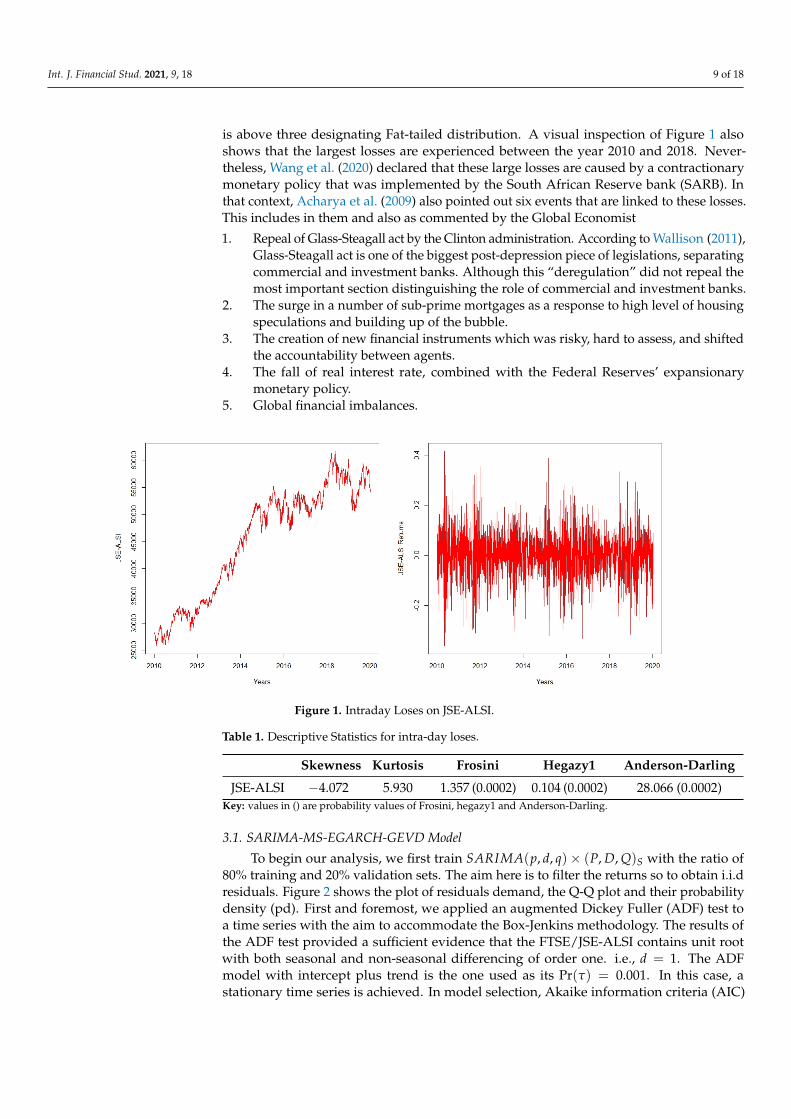
is above three designating Fat-tailed distribution. A visual inspection of Figure 1 alsoshows that the largest losses are experienced between the year 2010 and 2018. Never-theless, Wang et al. (2020) declared that these large losses are caused by a contractionarymonetary policy that was implemented by the South African Reserve bank (SARB). Inthat context, Acharya et al. (2009) also pointed out six events that are linked to these losses.This includes in them and also as commented by the Global Economist

1. Repeal of Glass-Steagall act by the Clinton administration. According to Wallison (2011),Glass-Steagall act is one of the biggest post-depression piece of legislations, separatingcommercial and investment banks. Although this “deregulation” did not repeal themost important section distinguishing the role of commercial and investment banks.

2. The surge in a number of sub-prime mortgages as a response to high level of housingspeculations and building up of the bubble.

3. The creation of new financial instruments which was risky, hard to assess, and shiftedthe accountability between agents.

4. The fall of real interest rate, combined with the Federal Reserves’ expansionarymonetary policy.

5. Global financial imbalances.

Figure 1. Intraday Loses on JSE-ALSI.

Table 1. Descriptive Statistics for intra-day loses.

Skewness Kurtosis Frosini Hegazy1 Anderson-Darling

JSE-ALSI −4.072 5.930 1.357 (0.0002) 0.104 (0.0002) 28.066 (0.0002)Key: values in () are probability values of Frosini, hegazy1 and Anderson-Darling.

3.1. SARIMA-MS-EGARCH-GEVD Model

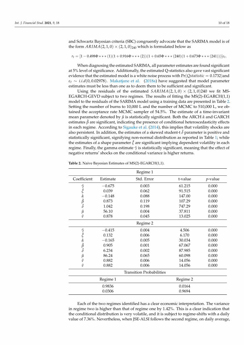
To begin our analysis, we first train SARIMA(p, d, q)× (P, D, Q)S with the ratio of80% training and 20% validation sets. The aim here is to filter the returns so to obtain i.i.dresiduals. Figure 2 shows the plot of residuals demand, the Q-Q plot and their probabilitydensity (pd). First and foremost, we applied an augmented Dickey Fuller (ADF) test toa time series with the aim to accommodate the Box-Jenkins methodology. The results ofthe ADF test provided a sufficient evidence that the FTSE/JSE-ALSI contains unit rootwith both seasonal and non-seasonal differencing of order one. i.e., d = 1. The ADFmodel with intercept plus trend is the one used as its Pr(τ) = 0.001. In this case, astationary time series is achieved. In model selection, Akaike information criteria (AIC)

Int. J. Financial Stud. 2021, 9, 18 10 of 18

and Schwartz Bayesian criteria (SBC) congruently advocate that the SARIMA model is ofthe form ARIMA(2, 1, 0)× (2, 1, 0)240 which is formulated below as

rt = [1− 0.498Φ ∗ ∗ ∗ (1)(1 + 0.916Φ ∗ ∗ ∗ (2))(1 + 0.65Φ ∗ ∗ ∗ (240)(1 + 0.673Φ ∗ ∗ ∗ (241)))]εt.

When diagnosing the estimated SARIMA, all parameter estimates are found significantat 5% level of significance. Additionally, the estimated Q-statistics also gave vast significantevidence that the estimated model is a white noise process with Pr(Qstatistic = 0.1732)andεt ∼ i.i.d(0, 0.02978). Makatjane et al. (2018a) have suggested that model parameterestimates must be less than one as to deem them to be sufficient and significant.

Using the residuals of the estimated SARIMA(2, 1, 0) × (2, 1, 0)240 we fit MS-EGARCH-GEVD subject to two regimes. The results of fitting the MS(2)-EGARCH(1,1)model to the residuals of the SARIMA model using a training data are presented in Table 2.Setting the number of burns to 10,000 L and the number of MCMC to 510,000 L, we ob-tained the acceptance rate MCMC sampler of 54.5%. The estimate of a time-invariantmean parameter denoted by µ is statistically significant. Both the ARCH α and GARCHestimates β are significant, indicating the presence of conditional heteroscedasticity effectsin each regime. According to Sigauke et al. (2014), this implies that volatility shocks arealso persistent. In addition, the estimates of a skewed student-t δ parameter is positive andstatistically significant, signifying non-normal distribution as reported in Table 1; whilethe estimates of a shape parameter ξ are significant implying dependent volatility in eachregime. Finally, the gamma estimate γ is statistically significant, meaning that the effect ofnegative returns’ shocks on the conditional variance is higher returns.

Table 2. Naive Bayesian Estimates of MS(2)-EGARCH(1,1).

Regime 1

Coefficient Estimate Std. Error t-value p-value

γ −0.675 0.003 61.215 0.000ξ 0.039 0.062 91.515 0.000α −0.148 0.088 147.00 0.000β 0.873 0.119 107.29 0.000δ 1.042 0.198 747.29 0.000µ 56.10 0.004 37.811 0.000ν 0.878 0.045 13.025 0.000

Regime 2

γ −0.415 0.004 4.506 0.000ξ 0.132 0.006 6.170 0.000α −0.165 0.005 30.034 0.000β 0.905 0.001 67.067 0.000δ 6.234 0.002 87.985 0.000µ 86.24 0.065 60.098 0.000ν 0.882 0.006 14.056 0.000ν 0.882 0.006 14.056 0.000

Transition Probabilities

Regime 1 Regime 2

0.9836 0.01640.0306 0.9694

Each of the two regimes identified has a clear economic interpretation. The variancein regime two is higher than that of regime one by 1.42%. This is a clear indication thatthe conditional distribution is very volatile, and it is subject to regime-shifts with a dailyvalue of 7.36%. Nevertheless, when JSE-ALSI follows the second regime, on daily average,

Int. J. Financial Stud. 2021, 9, 18 11 of 18

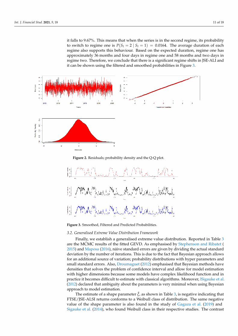
it falls to 9.67%. This means that when the series is in the second regime, its probabilityto switch to regime one is P(St = 2 | St = 1) = 0.0164. The average duration of eachregime also supports this behaviour. Based on the expected duration, regime one hasapproximately 36 months and four days in regime one and 58 months and two days inregime two. Therefore, we conclude that there is a significant regime shifts in JSE-ALI andit can be shown using the filtered and smoothed probabilities in Figure 3.

Figure 2. Residuals; probability density and the Q-Q plot.

Figure 3. Smoothed, Filtered and Predicted Probabilities.

3.2. Generalised Extreme Value Distribution Framework

Finally, we establish a generalised extreme value distribution. Reported in Table 3are the MCMC results of the fitted GEVD. As emphasised by Stephenson and Ribatet (2015) and Maposa (2016), näive standard errors are given by dividing the actual standarddeviation by the number of iterations. This is due to the fact that Bayesian approach allowsfor an additional source of variation; probability distributions with hyper parameters andsmall standard errors. Also, Droumaguet (2012) emphasised that Bayesian methods havedensities that solves the problem of confidence interval and allow for model estimationwith higher dimensions because some models have complex likelihood function and inpractice it becomes difficult to estimate with classical algorithms. Moreover, lSigauke et al.(2012) declared that ambiguity about the parameters is very minimal when using Bayesianapproach to model estimation.

The estimate of a shape parameter ξ, as shown in Table 3, is negative indicating thatFTSE/JSE-ALSI returns conforms to a Weibull class of distribution. The same negativevalue of the shape parameter is also found in the study of Gagaza et al. (2019) andSigauke et al. (2014), who found Weibull class in their respective studies. The contrast

Int. J. Financial Stud. 2021, 9, 18 12 of 18

is in the empirical analysis of Chan (2016) and Coles (2001), where the authors foundpositive shape parameters in their studies. In-addition, the 95% confidence interval forξ which is estimated using ξ ± zα/2 × (standarderror) has negative interval limits thatenclose the estimated shape parameter, hence confirming that the Weibull is an appropriatedistribution for FTSE/JSE-ALSI. Gagaza et al. (2019) in their study of modelling non-stationary temperature extremes in KwaZulu-Natal, using the generalised extreme valuedistribution, found the same negative limits. Furthermore, the right end point is µ− σ

ξ =1.377113, which implies that, with any degree losses above 25%, there is unlikely to be anyfurther decrease in JSE-ALSI losses.

Table 3. Naive Bayesian Estimates for Generalised Extreme Value Distribution (GEVD).

Block Minima ξ se(

ξ)

σ se(σ) µ0 se(µ0) 95% CI for ξ

JSE-ALSI 2400 482 −0.411 0.024 0.053 0.018 0.071 0.026 ( −0.459, −0.363 )

3.3. Comparative Analysis

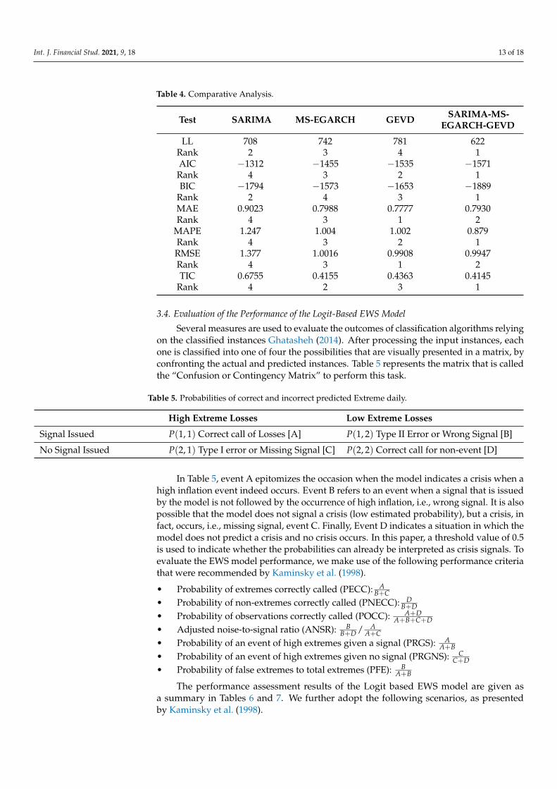
The purpose of this section is to determine the model which best mimics the data andproduces fewer forecasts. We therefore, use Akaike information criteria (AIC), SchwartzBayesian criteria (SBC), mean square error (MSE), mean absolute error (MAE) log-likelihood(LL) , mean absolute percentage error (MAPE) and Theil inequality (TIC) which are definedas statistical loss function. The well-known information criterion that are usually used formodel selection remain as the criterion used for prediction ability of the estimated models,that is, they are used here to select the model that best predicts the extreme losses. Whileon the other hand error metrics are used for the forecasting performance. For instance,the log-likelihood selected the best model as SARIMA-MS-EGARCH-GEVD while lookingat AIC; the best performing model was also selected as SARIMA-MS-EGARCH-GEVDwhile MAE and RMSE selected GEVD model as the best model. Therefore, Raihan (2017)in his study, ranked the models according to their statistical loss functions to overcomecontradicting results. The author used 10 statistical loss functions. Following this author,we only used seven statistical loss functions and the models were ranked from 1 to 4. Onthat note, rank 1 denoted the best model while 3 denoted the poorest model. Table 4 gavemuch evidence that SARIMA model has the poorest performance, as the frequency ofrank 4 is higher than the other three models by looking at their statistical loss functions.Nevertheless, the SARIMA-MS-EGARCH-GEVD model outperformed all the models, asthe frequency of rank 1 was higher than the other three models as it recorded 5 out of 7statistical loss functions.

Int. J. Financial Stud. 2021, 9, 18 13 of 18

Table 4. Comparative Analysis.

Test SARIMA MS-EGARCH GEVD SARIMA-MS-EGARCH-GEVD

LL 708 742 781 622Rank 2 3 4 1AIC −1312 −1455 −1535 −1571Rank 4 3 2 1BIC −1794 −1573 −1653 −1889

Rank 2 4 3 1MAE 0.9023 0.7988 0.7777 0.7930Rank 4 3 1 2

MAPE 1.247 1.004 1.002 0.879Rank 4 3 2 1RMSE 1.377 1.0016 0.9908 0.9947Rank 4 3 1 2TIC 0.6755 0.4155 0.4363 0.4145

Rank 4 2 3 1

3.4. Evaluation of the Performance of the Logit-Based EWS Model

Several measures are used to evaluate the outcomes of classification algorithms relyingon the classified instances Ghatasheh (2014). After processing the input instances, eachone is classified into one of four the possibilities that are visually presented in a matrix, byconfronting the actual and predicted instances. Table 5 represents the matrix that is calledthe “Confusion or Contingency Matrix” to perform this task.

Table 5. Probabilities of correct and incorrect predicted Extreme daily.

High Extreme Losses Low Extreme Losses

Signal Issued P(1, 1) Correct call of Losses [A] P(1, 2) Type II Error or Wrong Signal [B]

No Signal Issued P(2, 1) Type I error or Missing Signal [C] P(2, 2) Correct call for non-event [D]

In Table 5, event A epitomizes the occasion when the model indicates a crisis when ahigh inflation event indeed occurs. Event B refers to an event when a signal that is issuedby the model is not followed by the occurrence of high inflation, i.e., wrong signal. It is alsopossible that the model does not signal a crisis (low estimated probability), but a crisis, infact, occurs, i.e., missing signal, event C. Finally, Event D indicates a situation in which themodel does not predict a crisis and no crisis occurs. In this paper, a threshold value of 0.5is used to indicate whether the probabilities can already be interpreted as crisis signals. Toevaluate the EWS model performance, we make use of the following performance criteriathat were recommended by Kaminsky et al. (1998).

• Probability of extremes correctly called (PECC): AB+C

• Probability of non-extremes correctly called (PNECC): DB+D

• Probability of observations correctly called (POCC): A+DA+B+C+D

• Adjusted noise-to-signal ratio (ANSR): BB+D / A

A+C• Probability of an event of high extremes given a signal (PRGS): A

A+B• Probability of an event of high extremes given no signal (PRGNS): C

C+D• Probability of false extremes to total extremes (PFE): B

A+B

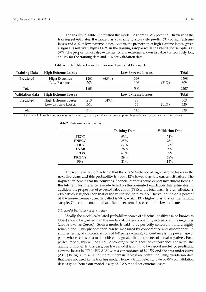
The performance assessment results of the Logit based EWS model are given asa summary in Tables 6 and 7. We further adopt the following scenarios, as presentedby Kaminsky et al. (1998).

Int. J. Financial Stud. 2021, 9, 18 14 of 18

The results in Table 6 infer that the model has some EWS potential. In view of thetraining set estimates, the model has a capacity to accurately predict 63% of high extremelosses and 21% of low extreme losses. As it is, the proportion of high extreme losses, givena signal, is relatively high at 43% in the training sample while the validation sample is at57%. The proportion of false extremes to total extremes shown in Table 7 is relatively low,at 21% for the training data and 14% for validation data.

Table 6. Probabilities of correct and incorrect predicted Extreme daily.

Training Data High Extreme Losses Low Extreme Losses Total

Predicted High Extremes 1200 (63% ) 398 1598Low Extremes 703 106 (21%) 809

Total 1903 504 2407

Validation data High Extreme Losses Low Extreme Losses Total

Predicted High Extreme Losses 210 (51%) 99 309Low extreme Losses 204 16 (14%) 220

Total 414 115 529The first set of numbers represents counts while figures in parentheses represent percentages of correctly predicted extreme losses.

Table 7. Performance of the EWS.

Training Data Validation Data

PECC 63% 51%PNECC 85% 98%POCC 67% 86%ANSR 78% 99%PRGS 43 % 57%

PRGNS 29% 48%PFE 21% 14%

The results in Table 7 indicate that there is 51% chance of high extreme losses in thenext five years and this probability is about 12% lower than the current situation. Theimplication here is that the countries’ financial markets could expect investment losses inthe future. This inference is made based on the presented validation data estimates. Inaddition, the proportion of expected false alarm (PFE) to the total alarm is premeditated as21% which is higher than that of the validation data by 7%. The validation data percentof the non-extremes correctly called is 98%, which 13% higher than that of the trainingsample. One could conclude that, after all, extreme losses could be low in future.

3.5. Model Performance Evaluation

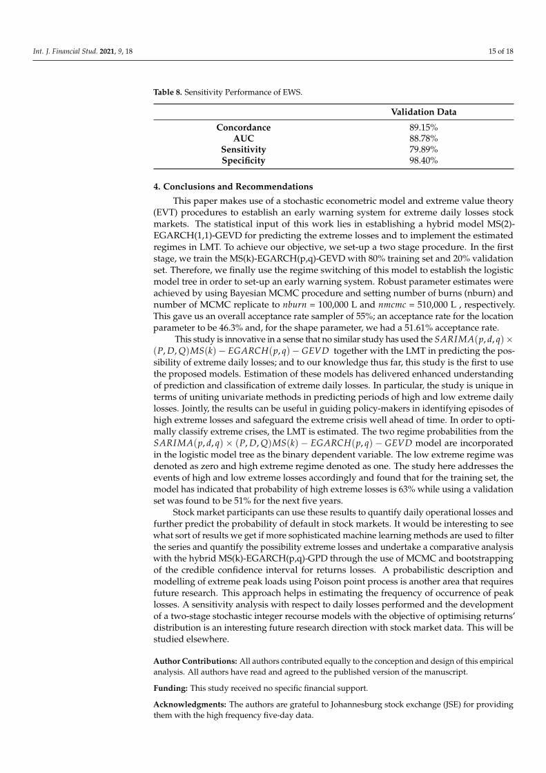
Ideally, the model-calculated-probability-scores of all actual positives (also known asOnes) should be greater than the model-calculated-probability-scores of all the negatives(also known as Zeroes). Such a model is said to be perfectly concordant and a highlyreliable one. This phenomenon can be measured by concordance and discordance. Insimpler terms, of all combinations of 1–0 pairs (actuals), concordance is the percentage ofpairs, whose scores of actual positives are greater than the scores of actual negatives. For aperfect model, this will be 100%. Accordingly, the higher the concordance, the better thequality of model. In this case, our EWS model is found to be a good model for predictingextreme losses in FTSE/JSE-ALSI with a concordance of 89.15% and the area under curve(AUC) being 88.78%. All of the numbers in Table 8 are computed using validation datathat were not used in the training model Hence, a truth detection rate of 79% on validationdata is good, hence our model is a good EWS model for extreme losses.

Int. J. Financial Stud. 2021, 9, 18 15 of 18

Table 8. Sensitivity Performance of EWS.

Validation Data

Concordance 89.15%AUC 88.78%

Sensitivity 79.89%Specificity 98.40%

4. Conclusions and Recommendations

This paper makes use of a stochastic econometric model and extreme value theory(EVT) procedures to establish an early warning system for extreme daily losses stockmarkets. The statistical input of this work lies in establishing a hybrid model MS(2)-EGARCH(1,1)-GEVD for predicting the extreme losses and to implement the estimatedregimes in LMT. To achieve our objective, we set-up a two stage procedure. In the firststage, we train the MS(k)-EGARCH(p,q)-GEVD with 80% training set and 20% validationset. Therefore, we finally use the regime switching of this model to establish the logisticmodel tree in order to set-up an early warning system. Robust parameter estimates wereachieved by using Bayesian MCMC procedure and setting number of burns (nburn) andnumber of MCMC replicate to nburn = 100,000 L and nmcmc = 510,000 L , respectively.This gave us an overall acceptance rate sampler of 55%; an acceptance rate for the locationparameter to be 46.3% and, for the shape parameter, we had a 51.61% acceptance rate.

This study is innovative in a sense that no similar study has used the SARIMA(p, d, q)×(P, D, Q)MS(k)− EGARCH(p, q)− GEVD together with the LMT in predicting the pos-sibility of extreme daily losses; and to our knowledge thus far, this study is the first to usethe proposed models. Estimation of these models has delivered enhanced understandingof prediction and classification of extreme daily losses. In particular, the study is unique interms of uniting univariate methods in predicting periods of high and low extreme dailylosses. Jointly, the results can be useful in guiding policy-makers in identifying episodes ofhigh extreme losses and safeguard the extreme crisis well ahead of time. In order to opti-mally classify extreme crises, the LMT is estimated. The two regime probabilities from theSARIMA(p, d, q) × (P, D, Q)MS(k) − EGARCH(p, q) − GEVD model are incorporatedin the logistic model tree as the binary dependent variable. The low extreme regime wasdenoted as zero and high extreme regime denoted as one. The study here addresses theevents of high and low extreme losses accordingly and found that for the training set, themodel has indicated that probability of high extreme losses is 63% while using a validationset was found to be 51% for the next five years.

Stock market participants can use these results to quantify daily operational losses andfurther predict the probability of default in stock markets. It would be interesting to seewhat sort of results we get if more sophisticated machine learning methods are used to filterthe series and quantify the possibility extreme losses and undertake a comparative analysiswith the hybrid MS(k)-EGARCH(p,q)-GPD through the use of MCMC and bootstrappingof the credible confidence interval for returns losses. A probabilistic description andmodelling of extreme peak loads using Poison point process is another area that requiresfuture research. This approach helps in estimating the frequency of occurrence of peaklosses. A sensitivity analysis with respect to daily losses performed and the developmentof a two-stage stochastic integer recourse models with the objective of optimising returns’distribution is an interesting future research direction with stock market data. This will bestudied elsewhere.

Author Contributions: All authors contributed equally to the conception and design of this empiricalanalysis. All authors have read and agreed to the published version of the manuscript.

Funding: This study received no specific financial support.

Acknowledgments: The authors are grateful to Johannesburg stock exchange (JSE) for providingthem with the high frequency five-day data.

Int. J. Financial Stud. 2021, 9, 18 16 of 18

Conflicts of Interest: The authors declare that they have no competing interests.

AbbreviationsThe following abbreviations are used in this manuscript:

ANSR Adjusted Noise-to-Signal RatioAUC Area Under CurveCART Classification and Regression TreeEWS Early Warning SystemEVT Extreme Value TheoryFTSE/JSE-ALSI Financial Time Series exchange/Johannesburg Stock Exchange- All Share IndexGARCH Generalised Autoregressive Conditional HeteroscedasticityGEVD Generalised Extreme Value DistributionGPD Generalised Pareto Distributioni.i.d Independent and identically distributedJSE-ALSI Johannesburg Stock Exchange-All share indexLMT Logistic Model TreeMC Markov-chainMCMC Markov-chain-Monte-CarloMS-EGARCH-GEVD

Markov-Switching Exponential Generalised Autoregressive ConditionalHeteroscedasticity-Generalised Extreme Value Distribution

MS-EGARCH-GEVD

Markov-Switching Exponential Generalised Autoregressive ConditionalHeteroscedasticity-Generalised Pareto Distribution

MS-GARCH Markov-Switching Generalised Autoregressive Conditional HeteroscedasticityPD Probability DensityPECC Probability of Extremes Correctly CalledPFE Probability of False Extremes to Total ExtremesPNECC Probabilty of Non-Extremes Correctly CalledPOCC Probability of Observations Correctly CalledPRGS Probability of an Extreme Event Given SignalPRSNS Probability of Event of High Extremes Given no SignalSARIMA-MS-EGARCH-GEVD

Seasonal Autoregressive Integrated Moving Average-Markov-switching Expo-nential Generalised Autoregressive Conditional Heteroscedasticity-GeneralisedExtreme Value Distribution

Q-Q Quantile-Quantile

ReferencesAbiad, Abdul. 2003. Early Warning Systems: A Survey and a Regime-Switching Approach (EPub). Financial Markets, Institutions and

Instruments 18: 89–137. [CrossRef]Acharya, Viral, Thomas Philippon, Matthew Richardson, and Nouriel Roubini. 2009. The Financial Crisis of 2007–2009: Causes and

Remedies. Financial Markets, Institutions and Instruments 18: 89–137. [CrossRef]Agresti, Alan. 2018. An Introduction to Categorical Data Analysis. Hoboken: John Wiley and Sons.Ardia, David, Keven Bluteau, Kris Boudt, and Leopoldo Catania. 2018. Forecasting Risk with Markov-Switching GARCH Models: A

large-scale Performance Study. International Journal of Forecasting 34: 733–47. [CrossRef]Ardia, David, Keven Bluteau, Kris Boudt, Leopoldo Catania, and Denis-Alexandre Trottier. 2016. Markov-Switching GARCH Models

in R: The MSGARCH Package. Journal of Statistical Software. [CrossRef]Arias, Guillaume, and Ulf Erlandsson. 2004. Regime Switching as an Alternative Early Warning System of Currency Crises—An

application to South-East Asia. Working Papers, Department of Economics, School of Economics and Management, LundUniversity, Lund, Sweden. Available online: https://lup.lub.lu.se/record/1387367 (accessed on 8 March 2021).

Bauwens, Luc, Bruno De Backer, and Arnaud Dufays. 2014. Bayesian Method of Change Point Estimation with Recurrent Regimes:Application to GARCH Models. Journal of Empirical Finance 29: 207–29. [CrossRef]

Bee, Macro. 2012. Dynamic Value-at-Risk Models and the Peaks-Over-Threshold Method for Market Risk Measurement: An EmpiricalInvestigation During a Financial Crisis. The Journal of Risk Model Validation 6: 2. [CrossRef]

Bee, Marco, and Luca Trapin. 2018. Estimating and Forecasting Conditional Risk Measures with Extreme Value Theory: A Review.Risks 6: 45. [CrossRef]

Bekaert, Geert, Michael Ehrmann, Marcel Fratzscher, and Arnaud Mehl. 2014. The Global Crises and Equity Market Contagion. TheJournal of Finance 69: 2597–649. [CrossRef]

Int. J. Financial Stud. 2021, 9, 18 17 of 18

Billio, Monica, Roberto Casarin, and Anthony Osuntuyi. 2018. Markov-Switching GARCH Models for Bayesian Hedging on EnergyFutures Markets. Energy Economics 70: 545–62. [CrossRef]

Borio, Claudio E. V., and Mathias Drehmann. 2009. Assessing the Risk of Banking Crises—Revisited. BIS Quarterly Review 29: 29–46.Box, George E. P., Gwilym M. Jenkins, Gregory C. Reinsel, and Greta M. Ljung. 2015. Time Series Analysis: Forecasting and Control.

Hoboken: John Wiley and Sons.Bui, Dieu Tien, Tran Anh Tuan, Harald Klempe, Biswajeet Pradhan, and Inge Revhaug. 2016. Spatial Prediction Models for Shallow

Landslide Hazards: A Comparative Assessment of the Efficacy of Support Vector Machines, Artificial Neural Networks, KernelLogistic Regression, and Logistic Model Tree. Landslides 13: 361–78. [CrossRef]

Chan, K. S. 2016. Statistical Modelling of Extreme Values for Dependent Variables. Master’s thesis, South Korea University, Seoul, Korea.Calabrese, Raffaella, and Paolo Giudici. 2015. Estimating Bank Default with Generalised Extreme Value Regression Model. Journal of

the Operational Research Society 66: 1783–92. [CrossRef]Carriero, Andrea, Todd E. Clark, and Massimiliano Marcellino. 2015. Bayesian VARS: Specification Choices and Forecast Accuracy.

Journal of Applied Econometrics 30: 46–73. [CrossRef]Chen, Wei, Xiaoshen Xie, Jiale Wang, Biswajeet Pradhan, Haoyuan Hong, Dieu Tien Bui, Zhao Duan, and Jianquan Ma. 2017. A

Comparative Study of Logistic Model Tree, Random Forest, and Classification and Regression Tree Models for Spatial Predictionof Landslide Susceptibility. Catena 51: 147–60. [CrossRef]

Chinhamu, Knowledge, Chun-Kai Huang, Chun-Sung Huang, and Delson Chikobvu. 2015. Extreme Risk, Value-at-Risk and ExpectedShortfall in the Gold Market. The International Business and Economics Research Journal (IBER) 14: 107–22. [CrossRef]

Cruz, Christopher John, and Dennis Mapa. 2013. An Early Warning System for Inflation in the Philippines Using Markov-Switchingand Logistic Regression Models. Theoretical and Practical Research in Economic Fields (TPREF). 8: 137–52. [CrossRef]

Coles, Stuart. 2001. An Introduction to Statistical Modelling of Extreme Values. London: Springer. [CrossRef]Davis, Philip, and Dilruba Karim. 2008. Comparing Early Warning Systems for Banking Crises. Journal of Financial Stability 4: 89–120.

[CrossRef]Diebold, Francis X. 2015. Perspective on the Use and Abuse of Diebold Mariano Tests. Journal of Business and Economic Statistics 33:

1–18. [CrossRef]Doetsch, Patrick, Christian Buck, Pavlo Golik, Niklas Hoppe, Michael Kramp, Johannes Laudenberg, Christian Oberdörfer, Pascal

Steingrube, Jens Forster, and Arne Mauser. 2009. Logistic Model Trees with AUC Split Criterion for the KDD Cup 2009 SmallChallenge. In KDD-Cup 2009 Competition. Aachen: Human Language Technology and Pattern Recognition, vol. 7, pp. 77–88.

Droumaguet, Matthieu. 2012. Markov-Switching Vector Autoregressive Models: Monte Carlo Experiment, Impulse Response Analysis,and Granger-Causal. Ph.D. thesis, Department of Economics, European University Institute, San Domenico di Fiesole, Italy.

Edison, Hali. 2002. Do Indicators of Financial Crises Work? An Evaluation of an Early Warning System. An Evaluation of an EarlyWarning System. International Journal of Finance and Economics 8: 11–53. [CrossRef]

Forbes, Kristin J., and Roberto Rigobon. 2002. No contagion, only interdependence: Measuring stock market co-movements. TheJournal of Finance.57: 2223–61. [CrossRef]

Fuertes, Ana-Maria, and Elena Kalotychou. 2007. Optimal Design of Early Warning Systems for Sovereign Debt Crises. InternationalJournal of Forecasting 23: 85–100. [CrossRef]

Gagaza, Nceba, Murendeni Maurel Nemukula, Retius Chifurira, and Danielle Jade Roberts. 2019. Modelling Non-stationaryTemperature Extremes in KwaZulu-Natal using the Generalised Extreme Value Distribution. In Annual Proceedings of the SouthAfrican Statistical Association Conference. Port Elizabeth: Nelson Mandela Metropolitan University, pp. 1–8.

Ghatasheh, Nzaeeh. 2014. Business Analytics using Random Forest Trees for Credit Risk Prediction: A Comparison Study. InternationalJournal of Advanced Science and Technology 72: 19–30. [CrossRef]

Heffernan, Janet E., Alec G. Stephenson, and Eric Gilleland. 2018. Ismev: An Introduction to Statistical Modelling of Extreme Values,R Package Version 1. Journal of Statistical Software. Available online: http://cran.rediris.es/web/packages/ismev/ismev.pdf(accessed on 8 March 2021).

Jeanne, Olivier, and Paul Masson. 2000. Currency Crises, Sunspots and Markov-Switching Regimes.Journal of International Economics50: 327–50. [CrossRef]

Kamarudin, Muhammad Hilmi, Carsten Maple, Tim Watson, and Nader Sohrabi Safa. 2017. A Logitboost-Based Algorithm forDetecting Known and Unknown Web Attacks. IEEE 5: 26190–200. [CrossRef]

Kaminsky, Graciela, Saul Lizondo, and Carmen M. Reinhart. 1998. Leading Indicators of Currency Crises.Staff Papers 45: 1–48.[CrossRef]

Kolari, James, Dennis Glennon, Hwan Shin, and Michele Caputo. 2002. Predicting Large US Commercial Bank Failures. Journal ofEconomics and Business 54: 361–87. [CrossRef]

Makatjane, Katleho Daniel, Edward Kagiso Molefe, and Roscoe Bertrum Van Wyk. 2018a. The Analysis of the 2008 US Financial Crisis:An Intervention Approach. Journal of Economics and Behavioural Studies 10: 59–68. [CrossRef]

Makatjane, Katleho, Ntebgoang Maroke, and Diteboho Xaba. 2018b. On the Prediction of Inflation Crises of South Africa usingMarkov-Switching Bayesian Vector Autoregressive and Logistic Regression Models. Journal of Social Economics Research 5: 10–28.[CrossRef]

Int. J. Financial Stud. 2021, 9, 18 18 of 18

Maposa, Daniel. 2016. Statistics of Extremes with Applications to Extreme Flood Heights in the Lower Limpopo River Basin ofMozambique. Ph.D. thesis, Department of Mathematics and Statistical Science, School of Mathematical Sciences, University ofLimpopo, Turfloop, South Africa.

Maposa, Daniel, Maseka Lesaoana, and James J. Cochran. 2016. Modelling Non-stationary Annual Maximum Flood Heights in theLower Limpopo River Basin of Mozambique. Jàmbá: Journal of Disaster Risk Studies 8: 1–9. [CrossRef]

Maposa, Daniel, James Cochran, Maseka Lesaoana, and Caston Sigauke. 2014. Estimating High Quantiles of Extreme Flood Heightsin the Lower Limpopo River Basin of Mozambique using Model based Bayesian Approach. Natural Hazards and Earth SystemSciences Discussions 2: 5401–25. [CrossRef]

Moroke, Ntebogang Dinah. 2014. The Robustness and Accuracy of Box-Jenkins ARIMA in Modelling and Forecasting Household Debtin South Africa. Journal of Economics and Behavioural Studies. 6: 748–59. [CrossRef]

Moysiadis, Theodoros, and Konstantnos Fokianos. 2014. On binary and Categorical Time Series Models with Feedback. Journal ofMultivariate Analysis 131: 209–28. [CrossRef]

Nemukula, Maurel Murendeni. 2018. Modelling Temperature in South Africa Using Extreme Value Theory. Ph.D. thesis, School ofStatistics and Actuarial Science, University of the Witwatersrand, Johannesburg, South Africa.

Pham, Binh Thai, and Indra Prakash. 2019. Evaluation and Comparison of Logitboost Ensemble, Fisher’s Linear Discriminant Analysis,Logistic Regression and Support Vector Machines Methods for Landslide Susceptibility Mapping. Geocarto International 34:316–33. [CrossRef]

Pourghasemi, Hamid Reza, Amiya Gayen, Sungjae Park, Chang-Wook Lee, and Saro Lee. 2018. Assessment of Landslide-prone Areasand their Zonation using Logistic Regression, Logitboost, and Naïve Bayes Machine-Learning Algorithms. Sustainability 10: 3697.[CrossRef]

Raihan, Tasneem. 2017. Perormance of Markov-Switching GARCH Model Forecasting Inflation Uncertainty. In Res-Report. Munich:University Library of Munich.

Schimmelpfennig, Axel, Nouriel Roubini, and Paolo Manasse. 2003. Predicting Sovereign Debt Crises. Washington, DC: InternationalMonetary Fund.

Sigaukea, Caston, Rhoda M. Makhwiting, and Maseka Lesaoana. 2014. Modelling Conditional Heteroscedasticity in JSE Stock Returnsusing the Generalised Pareto Distribution. African Review of Economics and Finance 6: 41–55.

Sigauke, Caston, André Verster, and Delson Chikobvu. 2012. Tail Quantile Estimation of Heteroscedastic Intraday Increases in PeakElectricity Demand. Open Journal of Statistics. 2: 435–42. [CrossRef]

Spyros, Makridakis. 1993. Accuracy Measures: Theoretical and Practical Concerns. International Journal of Forecasting 9: 527–29.[CrossRef]

Stephenson, Alec, and Mathieu Ribatet. 2015. evdbayes: Bayesian Analysis in Extreme Value Theory. Available online: https://cran.r-project.org/web/packages/evdbayes/evdbayes.pdf (accessed on 8 March 2021).

Stokes, Maura E., Charles S. Davis, and Gary G. Koch. 2012. Categorical Data Analysis Using SAS. Cary: SAS Institute.Theil, Henri. 1971. An Economic Theory of the Second Moments of Disturbance of Behavioural Equations. The American Economic

Review 61: 190–94.Troug, Hayatem, and Matt Murray. 2020. Crisis Determination and Financial Contagion: An Analysis of the Hong Kong and Tokyo

Stock Markets using an MSBVAR Approach. Journal of Economic Studies. [CrossRef]Tsay, Ruey. 2014. An Introduction to the Analysis of Financial Data with R. Hoboken: John Wiley and Sons.Wallison, Peter. 2011. Financial Market Regulation. In Did the Repeal of Glass-Steagall Have any Role in the Financial Crisis? Not Guilty.

Not Even Close. New York: Springer, pp. 19–29. [CrossRef]Wang, Lu, Feng Ma, Tianjiao Niu, and Chengting He. 2020. Crude Oil and BRICS Stock Markets under Extreme Shocks: New Evidence.

Economic Modelling 86: 54–68. [CrossRef]Zhang, Peter. 2010. Time Series Forecasting Using a Hybrid ARIMA and Neural Network Model. Neurocomputing 50: 159–75.

[CrossRef]