Predicting daily total ozone over Kolkata, India: skill assessment of different neural network models

METEOROLOGICAL APPLICATIONSMeteorol. Appl. 16: 179–190 (2009)Published online 7 October 2008 in Wiley InterScience(www.interscience.wiley.com) DOI: 10.1002/met.97

Predicting daily total ozone over Kolkata, India: skillassessment of different neural network models†

Goutami Chattopadhyaya and Surajit Chattopadhyayb*a Formerly, Department of Atmospheric Sciences, University of Calcutta, Kolkata 700019, India [Correction made here after initial publication.]

b Department of Information Technology, Pailan College of Management and Technology, Kolkata 700 104, India

ABSTRACT: This paper explores the observation made by the Earth Probe Total Ozone Mapping Spectrometer (EP/TOMS)to analyse the predictability of daily total ozone concentration over Kolkata, India. Latitude, longitude, aerosol index,reflectivity, sulphur dioxide index and total ozone concentration of a given day have been used as independent variablesto predict total ozone concentration of the next day. Artificial neural network in the forms of a multilayer perceptron,generalized feed forward neural network, a radial basis function network and a modular neural network have been trainedto generate predictive models. Performances of the models in the test cases have been judged with the help of four statisticalparameters. Finally the models have been compared with multiple linear regression and the potential of generalized feedforward neural network has been established over the other proposed models. Copyright 2008 Royal MeteorologicalSociety

KEY WORDS total ozone concentration; multilayer perceptron; generalized feed forward neural network; radial basis functionnetwork; modular neural network; regression; prediction

Received 6 April 2008; Revised 3 July 2008; Accepted 14 July 2008

1. Introduction

The role of ozone in the tropospheric-surface energybalance (Ramanathan and Dickinson, 1979; TIAHDAG,2005) and the importance of forecasting surface ozoneconcentration levels have been discussed in various lit-erature (e.g. Gaza, 1998; USEPA, 1999). Ozone at analtitude of 10–40 km in the atmosphere is vitally impor-tant because it protects the Earth from dangerous UVradiation from the Sun (Kondratyev et al., 1995; Varot-sos et al., 1995, 2003). On the other hand, when ozoneis close to the ground in higher concentrations (greaterthan 68 ppb), it is damaging to human health (Amannand Lutz, 2000). Due to the intrinsic spatial and temporalinconsistency of emission concentrations, the influence ofweather conditions, and uncertainties associated with ini-tial and boundary conditions, it is very difficult to model,calibrate and validate ozone variations from first princi-ples (Chen et al., 1998). A multidimensional phase spacemap was created by Chen et al. (1998) from observedozone concentration and a powerful predictive model wasdeveloped therein by examining trajectories on a recon-structed phase space for hourly ozone time series. Kocaket al. (2000) adopted a non-linear approach to develop apredictive model for the ozone time series through the

* Correspondence to: Surajit Chattopadhyay, Department of Informa-tion Technology, Pailan College of Management and Technology,Kolkata 700 104, India. E-mail: surajit [email protected]† This article was published online on 7 October 2008. An error wassubsequently identified. This notice is included in the online and printversions to indicate that both have been corrected, 20 January 2009.

method of phase-space reconstruction and identified thepresence of deterministic chaos within the ozone timeseries. Novara et al. (2007) approached the problem offorecasting tropospheric ozone concentration by meansof non-linear black-box modelling techniques.

Total ozone (TO) is defined as being equal to the num-ber of ozone molecules in a vertical column whose areaat the ground is 1 cm2 at standard temperature (0 °C) andpressure (1000 hPa; sea level) or STP. The TO, whichincludes the ozone present in the stratospheric ozonelayer and that present throughout the troposphere is mea-sured in Dobson Units (DU). One DU means 10−3 cmof column ozone at STP (for details see Reid, 2000).Climate change influences the evolution of the ozonelayer (a region of the stratosphere between 15 and 30 kmin altitude containing a relatively high concentration ofozone) through changes in transport, chemical composi-tion and temperature (Reid et al., 1994; Varotsos et al.,2004). In turn, changes to the ozone layer affect theclimate through radiative processes, and consequentialchanges in temperature gradients affect the atmosphericdynamics. Therefore, climate change and the evolutionof the ozone layer are highly correlated. Understandingall of the processes involved in these dynamics is highlycomplex because many of the interactions are non-linear.The climate–ozone interaction has been discussed exten-sively by Baldwin et al. (2006). The complexity in thetropospheric ozone has been thoroughly discussed by Efs-tathiou et al. (2003) and Kondratyev and Varotsos (2002).During the last few decades, study of TO has gainedimmense importance not only for the communities of

Copyright 2008 Royal Meteorological Society

180 G. CHATTOPADHYAY AND S. CHATTOPADHYAY

climatologists and meteorologists but also for biologyand medicine-related areas (Monge-Sanz and Medrano-Marques, 2003).

The sources of complexity in TO study have beendiscussed by Firor (1990); Chen et al. (1998); Monks(2003); Bourqui et al. (2005); Zai and Khan (2006);Chattopadhyay and Bandyopadhyay (2007) and manyothers. The relation between aerosol and total ozonehas been extensively studied over the years (e.g. Varot-sos, 2005). Nevertheless, the mechanisms that drive theozone–aerosol (liquid and solid particle) interactions arenot yet well understood, although there is observationalevidence on the dependence of the solid aerosol reactiv-ity on the aerosol composition and their physicochemicalproperties that vary with air pressure and temperature(Varotsos, 1978, 1980; Varotsos and Alexopoulos, 1980;Lazaridou et al., 1985).

Various mathematical approaches have been adoptedto deal with the complex processes associated with theformation of TO (see William et al. (2002) and referencestherein). Detrended fluctuation analysis, a method fordetermining the statistical self-affinity of a signal, hasbeen applied to the time series of the atmospheric ozoneand CO2 concentration data (Varotsos, 2005; Varotsoset al., 2007). Varotsos and Cracknell (2004) appliedsimilar numerical models to analyze solar activity andglobal total ozone dynamics. A statistical method forforecasting total column ozone was developed by Austinet al. (1994), extending the method of Poulin and Evans(1994).

An Artificial Neural Network (ANN) is a multiproces-sor computer system based on the parallel architecture ofthe brain and is useful in the situations where underlyingprocesses or relationships may display chaotic properties(Maqsood et al., 2002). An ANN does not require anyprior knowledge of the system under consideration and iswell suited to model dynamic systems on a real-time basis(Maqsood et al., 2002). ANNs are widely used to predicttime series pertaining to various kinds of pollution-relatedproblems (e.g. Gardner and Dorling, 1998; Nunnari et al.,1998; Perez et al., 2000; Perez and Reyes, 2001; Corani,2005 and many others). Corani (2005) adopted an ANN,to form a pruned ANN, and Lazy Learning to pre-dict ozone and reported the suitability of all the modelsfor this prediction. Bandyopadhyay and Chattopadhyay(2007) and Chattopadhyay (2007) implemented artificialneural network methodology in the forms of multilayerperceptron and radial basis function to predict the totalozone time series and reported the potential of them overconventional regression approaches.

A plethora of literature is available where the asso-ciation between monsoon circulation and TO has beeninvestigated in the Indian context (e.g. Hingane and Patil,1996; Sathiyamoorthy et al., 2002; Londhe et al., 2003).Sahoo et al. (2005) applied a linear regression techniqueto the Nimbus and Earth Probe Total Ozone MappingSpectrometer (EP/TOMS) data to study the trends oftotal ozone over northern India during 1997–2003 andrevealed that the rate of decline of ozone was higher in

recent years over the northern parts of India, covering theIndo-Gangetic basin, compared with other parts of India.

In the present paper, Dum Dum, belonging to themega city Kolkata (formerly known as Calcutta) has beenchosen as the study zone. Significant literature is avail-able where the nature of the atmospheric environmentof Kolkata has been analyzed (e.g. Ghose et al., 2005;Londhe et al., 2005; Sahoo et al., 2005; Lal et al., 2006;Gupta et al., 2008). Kolkata is situated in Gangetic WestBengal, which is highly vulnerable to pre-monsoon thun-derstorms. The association between thunderstorms andozone has been studied by Poulida et al. (1996); Winter-rath et al. (1999) and Hauf et al. (1995). It is, therefore,felt that studies on the TO time series would be usefulin the research on thunderstorm and related events, giventhe atmospheric environment over Kolkata documentedin the literature mentioned earlier.

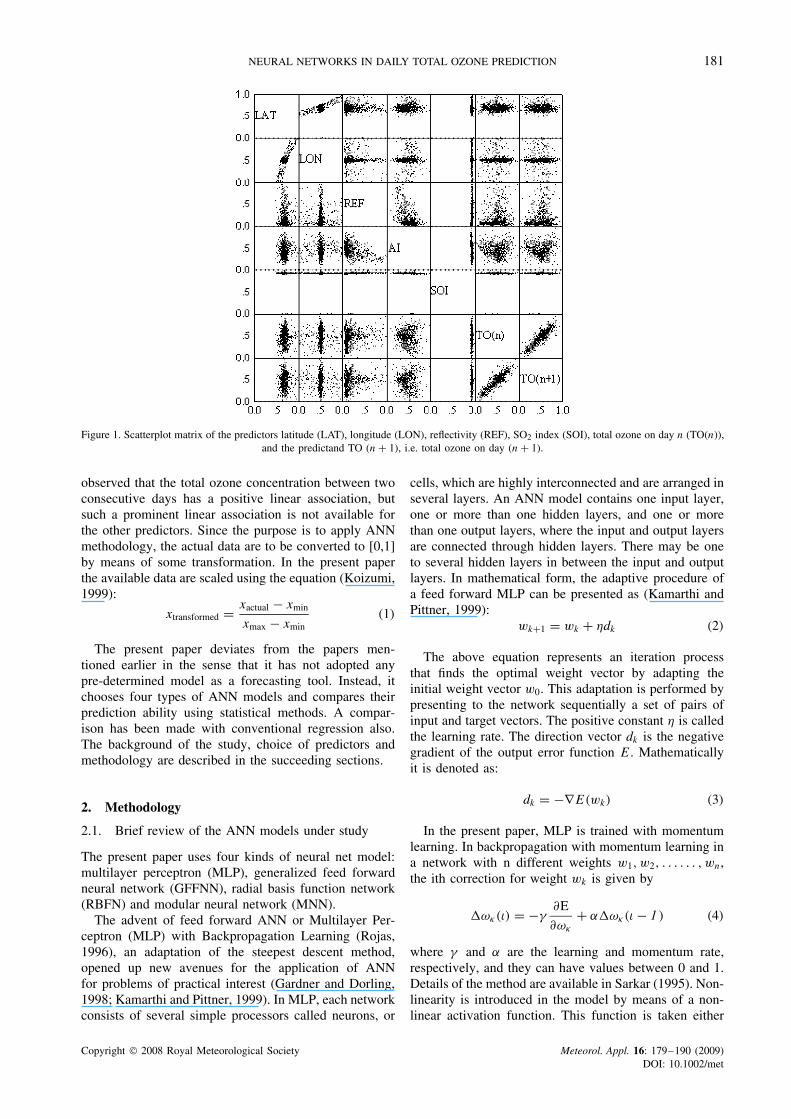
Datasets used in the present paper consist of themeasurements made by EP/TOMS available at the web-site ftp://jwocky.gsfc.nasa.gov/pub/eptoms/data/overpass/OVP075 epc.txt, which provides measurements ofEarth’s total column ozone by measuring the backscat-tered Earth radiance in the six 1 nm bands. The radiationdiffusely reflected by the terrestrial atmosphere comesmostly from a relatively thin layer, which is referred toas the effective scattering layer. The position of this layerdepends upon the ozone-absorbing power at the wave-length under consideration, the zenith angle of the Sunand vertical distribution of the total amount of ozone inthe atmosphere. If the diffusely reflected radiation is tocontain significant information on the total amount ofozone, most of the reflected radiation should have passedthrough and been attenuated by the major portion ofthe total atmospheric ozone. It follows that the effec-tive scattering layer should be located below the level ofmaximum ozone concentration (Dave and Materr, 1967).

The link between total ozone and aerosol is welldocumented (Dave, 1978; Bonasoni et al., 2004). Bekkiet al. (1993) found that a large amount of SO2 injectedinto the tropical atmosphere catalyses mid-stratosphericozone production, whilst the SO2 cloud reduces the rateof O2 photolysis by absorbing solar radiation (and hencereduces ozone production) below it. The associationbetween reflectivity and total ozone has been thoroughlydocumented by NASA (1998) and Hsu et al. (1997). Onthe basis of the ideas derived from these studies, latitude,longitude, solar zenith angle, reflectivity, aerosol index,SO2 index, and TO concentration on a given day havebeen used to predict the TO concentration of the nextday. The data pertain to 600 days of observations madeover the years 1996–1998. The study is based on theavailable dataset, so although the study period mentionedhere contains more than 900 days, only data pertainingto 600 days were available. All the said parameters fora given day are the predictors, and the predictand is thenext day’s total ozone concentration in DU. The typeof association between the predictors and the predictandis presented in terms of scatterplot matrix in Figure 1.From the last panel of this scatterplot matrix it is

Copyright 2008 Royal Meteorological Society Meteorol. Appl. 16: 179–190 (2009)DOI: 10.1002/met

NEURAL NETWORKS IN DAILY TOTAL OZONE PREDICTION 181

Figure 1. Scatterplot matrix of the predictors latitude (LAT), longitude (LON), reflectivity (REF), SO2 index (SOI), total ozone on day n (TO(n)),and the predictand TO (n + 1), i.e. total ozone on day (n + 1).

observed that the total ozone concentration between twoconsecutive days has a positive linear association, butsuch a prominent linear association is not available forthe other predictors. Since the purpose is to apply ANNmethodology, the actual data are to be converted to [0,1]by means of some transformation. In the present paperthe available data are scaled using the equation (Koizumi,1999):

xtransformed = xactual − xmin

xmax − xmin(1)

The present paper deviates from the papers men-tioned earlier in the sense that it has not adopted anypre-determined model as a forecasting tool. Instead, itchooses four types of ANN models and compares theirprediction ability using statistical methods. A compar-ison has been made with conventional regression also.The background of the study, choice of predictors andmethodology are described in the succeeding sections.

2. Methodology

2.1. Brief review of the ANN models under study

The present paper uses four kinds of neural net model:multilayer perceptron (MLP), generalized feed forwardneural network (GFFNN), radial basis function network(RBFN) and modular neural network (MNN).

The advent of feed forward ANN or Multilayer Per-ceptron (MLP) with Backpropagation Learning (Rojas,1996), an adaptation of the steepest descent method,opened up new avenues for the application of ANNfor problems of practical interest (Gardner and Dorling,1998; Kamarthi and Pittner, 1999). In MLP, each networkconsists of several simple processors called neurons, or

cells, which are highly interconnected and are arranged inseveral layers. An ANN model contains one input layer,one or more than one hidden layers, and one or morethan one output layers, where the input and output layersare connected through hidden layers. There may be oneto several hidden layers in between the input and outputlayers. In mathematical form, the adaptive procedure ofa feed forward MLP can be presented as (Kamarthi andPittner, 1999):

wk+1 = wk + ηdk (2)

The above equation represents an iteration processthat finds the optimal weight vector by adapting theinitial weight vector w0. This adaptation is performed bypresenting to the network sequentially a set of pairs ofinput and target vectors. The positive constant η is calledthe learning rate. The direction vector dk is the negativegradient of the output error function E. Mathematicallyit is denoted as:

dk = −∇E(wk) (3)

In the present paper, MLP is trained with momentumlearning. In backpropagation with momentum learning ina network with n different weights w1, w2, . . . . . . , wn,the ith correction for weight wk is given by

�ωκ(ι) = −γ∂E

∂ωκ

+ α�ωκ(ι − 1 ) (4)

where γ and α are the learning and momentum rate,respectively, and they can have values between 0 and 1.Details of the method are available in Sarkar (1995). Non-linearity is introduced in the model by means of a non-linear activation function. This function is taken either

Copyright 2008 Royal Meteorological Society Meteorol. Appl. 16: 179–190 (2009)DOI: 10.1002/met

182 G. CHATTOPADHYAY AND S. CHATTOPADHYAY

as a tanh function or as a sigmoidal function. Becauseof the advantageous form of derivative, the sigmoidalfunction is of more frequent use in development of MLPpredictive models. In the present paper, the sigmoidalfunction (Rojas, 1996) is adopted:

f (x) = (1 + e−x)−1 (5)

Generalized feedforward neural networks (GFFNN)are a generalization of the MLP such that connectionscan jump over one or more layers (Arulampalam andBouzerdoum, 2003; Bouzerdoum and Mueller, 2003).

Modularity is defined as a subdivision of a complexobject into simpler objects. The subdivision is determinedeither by the structure or by the function of the object andits subparts (Schmidt, 1996). Modular neural networks(MNN) (Ortin et al., 2005) are a particular class of MLP.These networks process their input using several paral-lel MLPs, and then recombine the results. This tends tocreate some structure within the topology, which will fos-ter specialization of function in each sub-module. Unlikethe MLP, modular networks do not have full interconnec-tivity between their layers. Therefore, a smaller numberof weights is required for the same size network. Thistends to speed up training times and reduce the numberof required training patterns. There are many ways tosegment an MLP into modules. In the present paper, thelearning for the MNN is also taken as the momentum, asfor the MLP, and the transfer function for all the parallelMLPs is taken as the sigmoid function (Equation (5)).

Radial basis function networks (RBFNs) are consid-ered as a subclass of Modular Neural Networks (MNNs).RBFNs are non-linear feed-forward networks. Their mostparticular characteristic is their architecture, which isbased on Radial Basis Function (RBF) activation units.Typical RBFNs are constructed by one hidden layer withRBF units and an output layer with only one linear neu-ron. The RBF layer uses Gaussian transfer functions,rather than the standard sigmoidal functions employedby MLPs. The output of the kth unit in the output layerof an RBFN is given by (Yegnanarayana, 2000):

bk′ =

J∑j=0

wkjhj (6)

where,hj = φj

(∥∥a − µj

∥∥ /σj

)(7)

The non-linear RBF φj (.) of the j th hidden unit is afunction of the normalized radial distance between theinput vector and the weight vector associated with theunit. In the present paper, the basis function has beentaken as Gaussian, i.e.

φ(x) = exp(−x2/2) (8)

After implementing all the ANN models to theEP/TOMS observations with observations pertaining to

day n as predictors, and daily total ozone concentrationon day (n + 1) as predictand, the performances of thenon-linear ANN models have been compared to a mul-tiple linear regression (MLR) model. The mathematicalform of MLR is

yi = w0 +n∑

i=1

wixi+ ∈ (9)

Where, yi implies the predicted value of the ith predic-tand, w0 denotes the regression constant, xi denoted theith predictor, wi denotes the regression parameter pertain-ing to the ith predictor, and ∈ is the error of prediction.

2.2. Evaluation of the performance of the models

Prediction performance of all the models is judged usingthe following statistical measurements (Chattopadhyayand Chattopadhyay-Bandyopadhyay, 2007):

• Willmott’s index of first order (W1);• Willmott’s index of second order (W2);• Overall prediction error (PE);• Pearson Correlation Coefficient (PCC).

Willmott (1982) advocated an index to measure thedegree of agreement between actual and predicted values.This is given as:

dα = 1 −[∑

i|Pi − Oi |α

]

×[∑

i(|Pi − O| + |Oi − O|)α

]−1(10)

where, α = 1 and 2, P implies predicted value and O

implies observed value. For α = 1 we get W1 and forα = 2 we get W2. For good predictive models, the W1and W2 are close to 1.

The overall prediction error (PE) is computed as:

PE =⟨∣∣ypredicted − yactual

∣∣⟩

〈yactual〉 × 100 (11)

The Pearson Correlation Coefficient (PCC) measuresthe degree of linear association between two variables.Mathematically it is written as:

ρxy = Covariance(x, y)

σxσy

(12)

where σx implies standard deviation of x and PCC ρ

lies between −1 and +1. When it is very close to +1, ahighly positive linear association is inferred. As much asthe actual and the prediction would be closely positivelyassociated, the PCC would come closer to +1. Similarly,for negative linear correlation, the PCC would be veryclose to −1. In other words, the correlation is high whenthe numerical value of PCC is very close to 1. In general,if the value of PCC is greater than 0.6, a good associationbetween actual and predicted values is inferred.

Copyright 2008 Royal Meteorological Society Meteorol. Appl. 16: 179–190 (2009)DOI: 10.1002/met

NEURAL NETWORKS IN DAILY TOTAL OZONE PREDICTION 183

3. Results and discussion

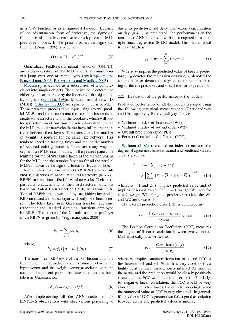
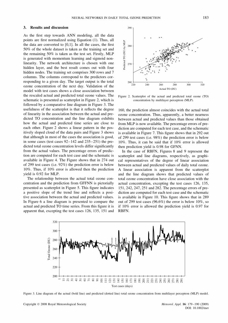
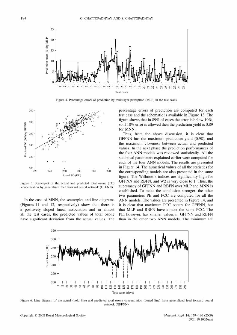
As the first step towards ANN modeling, all the datapoints are first normalized using Equation (1). Thus, allthe data are converted to [0,1]. In all the cases, the first50% of the whole dataset is taken as the training set andthe remaining 50% is taken as the test set. Firstly, MLPis generated with momentum learning and sigmoid non-linearity. The network architecture is chosen with onehidden layer, and the best result comes out with fourhidden nodes. The training set comprises 300 rows and 7columns. The columns correspond to the predictors cor-responding to a given day. The target output is the totalozone concentration of the next day. Validation of themodel with test cases shows a close association betweenthe rescaled actual and predicted total ozone values. Theschematic is presented as scatterplot in Figure 2, which isfollowed by a comparative line diagram in Figure 3. Theusefulness of the scatterplot is that it reflects the degreeof linearity in the association between the actual and pre-dicted TO concentration and the line diagram exhibitshow the actual and predicted time series are close toeach other. Figure 2 shows a linear pattern in the pos-itively sloped cloud of the data pairs and Figure 3 showsthat although in most of the cases the association is good,in some cases (test cases 92–142 and 235–251) the pre-dicted total ozone concentration levels differ significantlyfrom the actual values. The percentage errors of predic-tion are computed for each test case and the schematic isavailable in Figure 4. The Figure shows that in 274 outof 299 test cases (i.e. 92%) the prediction error is below10%. Thus, if 10% error is allowed then the predictionyield is 0.92 for MLP.

The relationship between the actual total ozone con-centration and the prediction from GFFNN is pictoriallypresented as scatterplot in Figure 5. This figure indicatesa positive slope of the trend line and reflects a posi-tive association between the actual and predicted values.In Figure 6 a line diagram is presented to compare theactual and predicted TO time series. From this figure it isapparent that, excepting the test cases 126, 135, 151 and

Actual TO (DU)

320300280260240220

Pred

icte

d T

O (

DU

) by

ML

P

290

280

270

260

Figure 2. Scatterplot of the actual and predicted total ozone (TO)concentration by multilayer perceptron (MLP).

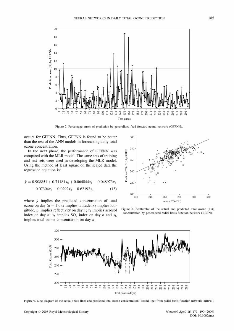
160, the prediction almost coincides with the actual totalozone concentration. Thus, apparently, a better nearnessbetween actual and predicted values than those obtainedfrom MLP is now available. The percentage errors of pre-diction are computed for each test case, and the schematicis available in Figure 7. This figure shows that in 292 outof 299 test cases (i.e. 98%) the prediction error is below10%. Thus, it can be said that if 10% error is allowedthen prediction yield is 0.98 for GFNN.

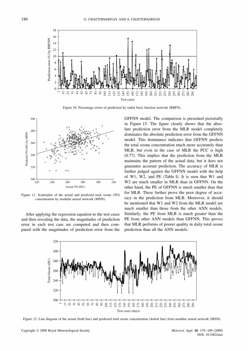
In the case of RBFN, Figures 8 and 9 represent thescatterplot and line diagrams, respectively, as graphi-cal representatives of the degree of linear associationbetween actual and predicted values of daily total ozone.A linear association is apparent from the scatterplotand the line diagram shows that predicted values oftotal ozone concentration have close association with theactual concentration, excepting the test cases 126, 135,151, 242, 247, 251 and 282. The percentage errors of pre-diction are computed for each test case and the schematicis available in Figure 10. This figure shows that in 289out of 299 test cases (96.6%) the error is below 10%, soif 10% error is allowed the prediction yield is 0.97 forRBFN.

200

220

240

260

280

300

320

1 11 21 31 41 51 61 71 81 91 101

111

121

131

141

151

161

171

181

191

201

211

221

231

241

251

261

271

281

291

Test cases (days)

Tot

al O

zone

(D

U)

Figure 3. Line diagram of the actual (bold line) and predicted (dotted line) total ozone concentration from multilayer perceptron (MLP) model.

Copyright 2008 Royal Meteorological Society Meteorol. Appl. 16: 179–190 (2009)DOI: 10.1002/met

184 G. CHATTOPADHYAY AND S. CHATTOPADHYAY

0

5

10

15

20

25

1 11 21 31 41 51 61 71 81 91 101

111

121

131

141

151

161

171

181

191

201

211

221

231

241

251

261

271

281

291

Test cases

Pred

ictio

n er

ror

(%)

by M

LP

Figure 4. Percentage errors of prediction by multilayer perceptron (MLP) in the test cases.

Actual TO (DU)

320300280260240220

Pred

icte

d T

O (

DU

) by

GFF

NN

300

280

260

240

220

200

Figure 5. Scatterplot of the actual and predicted total ozone (TO)concentration by generalized feed forward neural network (GFFNN).

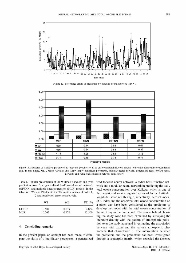
In the case of MNN, the scatterplot and line diagrams(Figures 11 and 12, respectively) show that there isa positively sloped linear association and in almostall the test cases, the predicted values of total ozonehave significant deviation from the actual values. The

percentage errors of prediction are computed for eachtest case and the schematic is available in Figure 13. Thefigure shows that in 89% of cases the error is below 10%,so if 10% error is allowed then the prediction yield is 0.89for MNN.

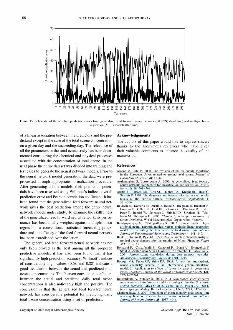
Thus, from the above discussion, it is clear thatGFFNN has the maximum prediction yield (0.98), andthe maximum closeness between actual and predictedvalues. In the next phase the prediction performances ofthe four ANN models was reviewed statistically. All thestatistical parameters explained earlier were computed foreach of the four ANN models. The results are presentedin Figure 14. The numerical values of all the statistics forthe corresponding models are also presented in the samefigure. The Willmott’s indices are significantly high forGFFNN and RBFN, and W2 is very close to 1. Thus, thesupremacy of GFFNN and RBFN over MLP and MNN isestablished. To make the conclusion stronger, the othertwo parameters PE and PCC are computed for all theANN models. The values are presented in Figure 14, andit is clear that maximum PCC occurs for GFFNN, butthat MLP and RBFN have almost the same PCC. ThePE, however, has smaller values in GFFNN and RBFNthan in the other two ANN models. The minimum PE

200

220

240

260

280

300

320

1 11 21 31 41 51 61 71 81 91 101

111

121

131

141

151

161

171

181

191

201

211

221

231

241

251

261

271

281

291

Test cases (days)

Tot

al O

zone

(D

U)

Figure 6. Line diagram of the actual (bold line) and predicted total ozone concentration (dotted line) from generalized feed forward neuralnetwork (GFFNN).

Copyright 2008 Royal Meteorological Society Meteorol. Appl. 16: 179–190 (2009)DOI: 10.1002/met

NEURAL NETWORKS IN DAILY TOTAL OZONE PREDICTION 185

0

2

4

6

8

10

12

14

16

18

20

1 11 21 31 41 51 61 71 81 91 101

111

121

131

141

151

161

171

181

191

201

211

221

231

241

251

261

271

281

291

Test cases

Pred

ictio

n er

ror

(%)

by G

FFN

N

Figure 7. Percentage errors of prediction by generalized feed forward neural network (GFFNN).

occurs for GFFNN. Thus, GFFNN is found to be betterthan the rest of the ANN models in forecasting daily totalozone concentration.

In the next phase, the performance of GFFNN wascompared with the MLR model. The same sets of trainingand test sets were used in developing the MLR model.Using the method of least square on the scaled data theregression equation is:

y = 0.908851 + 0.71181x6 + 0.064044x5 + 0.048973x4

− 0.07304x3 − 0.0292x2 − 0.62192x1 (13)

where y implies the predicted concentration of totalozone on day (n + 1); x1 implies latitude, x2 implies lon-gitude, x3 implies reflectivity on day n; x4 implies aerosolindex on day n; x5 implies SO2 index on day n and x6

implies total ozone concentration on day n.

Actual TO (DU)

320300280260240220

Pred

icte

d T

O (

DU

) by

RB

FN

300

280

260

240

220

200

Figure 8. Scatterplot of the actual and predicted total ozone (TO)concentration by generalized radial basis function network (RBFN).

200

220

240

260

280

300

320

1 11 21 31 41 51 61 71 81 91 101

111

121

131

141

151

161

171

181

191

201

211

221

231

241

251

261

271

281

291

Test cases (days)

Tot

al O

zone

(D

U)

Figure 9. Line diagram of the actual (bold line) and predicted total ozone concentration (dotted line) from radial basis function network (RBFN).

Copyright 2008 Royal Meteorological Society Meteorol. Appl. 16: 179–190 (2009)DOI: 10.1002/met

186 G. CHATTOPADHYAY AND S. CHATTOPADHYAY

0

2

4

6

8

10

12

14

16

18

1 11 21 31 41 51 61 71 81 91 101

111

121

131

141

151

161

171

181

191

201

211

221

231

241

251

261

271

281

291

Test cases

Pred

ictio

n er

ror

(%)

by R

BFN

N

Figure 10. Percentage errors of prediction by radial basis function network (RBFN).

Actual TO (DU)

320300280260240220

Pred

icte

d T

O (

DU

) by

MN

N

300

280

260

240

220

200

Figure 11. Scatterplot of the actual and predicted total ozone (TO)concentration by modular neural network (MNN).

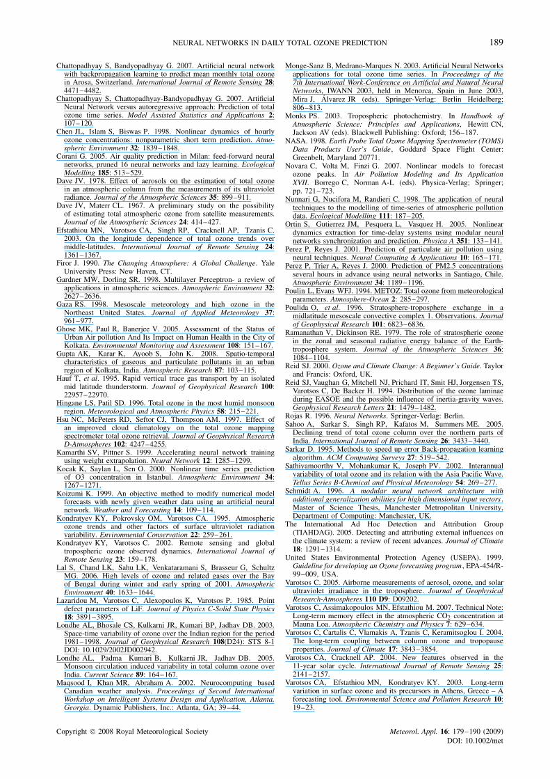
After applying the regression equation to the test casesand then rescaling the data, the magnitudes of predictionerror in each test case are computed and then com-pared with the magnitudes of prediction error from the

GFFNN model. The comparison is presented pictoriallyin Figure 15. The figure clearly shows that the abso-lute prediction error from the MLR model completelydominates the absolute prediction error from the GFFNNmodel. This dominance indicates that GFFNN predictsthe total ozone concentration much more accurately thanMLR, but even in the case of MLR the PCC is high(0.77). This implies that the prediction from the MLRmaintains the pattern of the actual data, but it does notguarantee accurate prediction. The accuracy of MLR isfurther judged against the GFFNN model with the helpof W1, W2, and PE (Table I). It is seen that W1 andW2 are much smaller in MLR than in GFFNN. On theother hand, the PE of GFFNN is much smaller than thatfor MLR. These further prove the poor degree of accu-racy in the prediction from MLR. Moreover, it shouldbe mentioned that W1 and W2 from the MLR model aremuch smaller than those from the other ANN models.Similarly, the PE from MLR is much greater than thePE from other ANN models than GFFNN. This provesthat MLR performs of poorer quality in daily total ozoneprediction than all the ANN models.

200

220

240

260

280

300

320

1 11 21 31 41 51 61 71 81 91 101

111

121

131

141

151

161

171

181

191

201

211

221

231

241

251

261

271

281

291

Test cases (days)

Tot

al O

zone

(D

U)

Figure 12. Line diagram of the actual (bold line) and predicted total ozone concentration (dotted line) from modular neural network (MNN).

Copyright 2008 Royal Meteorological Society Meteorol. Appl. 16: 179–190 (2009)DOI: 10.1002/met

NEURAL NETWORKS IN DAILY TOTAL OZONE PREDICTION 187

0

5

10

15

20

25

1 11 21 31 41 51 61 71 81 91 101

111

121

131

141

151

161

171

181

191

201

211

221

231

241

251

261

271

281

291

Test cases

Perd

ictio

n er

ror

(%)

by M

NN

Figure 13. Percentage errors of prediction by modular neural network (MNN).

Figure 14. Measures of statistical parameters to judge the goodness of fit of different neural network models to the daily total ozone concentrationdata. In this figure, MLP, MNN, GFFNN and RBFN imply multilayer perceptron, modular neural network, generalized feed forward neural

network, and radial basis function network respectively.

Table I. Tabular presentation of the Willmott’s indices and overprediction error from generalized feedforward neural network(GFFNN) and multiple linear regression (MLR) models. In thetable W1, W2 and PE denote the Willmott’s indices of order 1,

2 and prediction error, respectively.

W1 W2 PE (%)

GFFNN 0.684 0.879 2.824MLR 0.267 0.476 12.500

4. Concluding remarks

In the present paper, an attempt has been made to com-pare the skills of a multilayer perceptron, a generalized

feed forward neural network, a radial basis function net-work and a modular neural network in predicting the dailytotal ozone concentration over Kolkata, which is one ofthe largest and most congested cities of India. Latitude,longitude, solar zenith angle, reflectivity, aerosol index,SO2 index and the observed total ozone concentration ona given day have been considered as the predictors todevelop the model with the total ozone concentration ofthe next day as the predictand. The reason behind choos-ing the study zone has been explained by surveying theliterature dealing with the pattern of atmospheric pollu-tion over the study zone and investigating the associationbetween total ozone and the various atmospheric phe-nomena that characterize it. The interrelation betweenthe predictors and the predictand has been investigatedthrough a scatterplot matrix, which revealed the absence

Copyright 2008 Royal Meteorological Society Meteorol. Appl. 16: 179–190 (2009)DOI: 10.1002/met

188 G. CHATTOPADHYAY AND S. CHATTOPADHYAY

0

10

20

30

40

50

60

70

1 11 21 31 41 51 61 71 81 91 101

111

121

131

141

151

161

171

181

191

201

211

221

231

241

251

261

271

281

291

Test cases

Abs

olut

e pr

edic

tion

erro

r

Figure 15. Schematic of the absolute prediction errors from generalized feed forward neural network (GFFNN) (bold line) and multiple linearregression (MLR) models (thin line).

of a linear association between the predictors and the pre-dictand except in the case of the total ozone concentrationon a given day and the succeeding day. The relevance ofall the parameters in the total ozone study has been docu-mented considering the chemical and physical processesassociated with the concentration of total ozone. In thenext phase the entire dataset was divided into training andtest cases to generate the neural network models. Prior tothe neural network model generation, the data were pre-processed through appropriate normalization procedure.After generating all the models, their prediction poten-tials have been assessed using Willmott’s indices, overallprediction error and Pearson correlation coefficient. It hasbeen found that the generalized feed forward neural net-work gives the best prediction among the entire neuralnetwork models under study. To examine the skillfulnessof the generalized feed forward neural network, its perfor-mance has been finally weighed against multiple linearregression, a conventional statistical forecasting proce-dure and the efficacy of the feed forward neural networkhas been established over the latter.

The generalized feed forward neural network has notonly been proved as the best among all the proposedpredictive models, it has also been found that it hassignificantly high prediction accuracy. Willmott’s indicesof considerably high values (0.68 and 0.88) indicate agood association between the actual and predicted totalozone concentrations. The Pearson correlation coefficientbetween the actual and predicted daily total ozoneconcentrations is also noticeably high and positive. Theconclusion is that the generalized feed forward neuralnetwork has considerable potential for predicting dailytotal ozone concentration using a set of predictors.

Acknowledgements

The authors of this paper would like to express sincerethanks to the anonymous reviewers who have giventheir valuable comments to enhance the quality of themanuscript.

ReferencesAmann M, Lutz M. 2000. The revision of the air quality legislation

in the European Union related to ground-level ozone. Journal ofHazardous Materials 78: 41–62.

Arulampalam G, Bouzerdoum A. 2003. A generalized feed forwardneural network architecture for classification and regression. NeuralNetworks 16: 561–568.

Austin J, Barwell BR, Cox SJ, Hughes PA, Knight JR, Ross G,Sinclair P. 1994. The diagnosis and forecast of clear sky ultravioletlevels at the earth’s surface. Meteorological Applications 1:321–336.

Baldwin M, Dameris M, Austin J, Bekki S, Bregman B, Butchart N,Cordero E, Gillett N, Graf HF, Granier C, Kinnison D, Lal S,Peter T, Randel W, Scinocca J, Shindell D, Struthers H, Taka-hashi M, Thompson D. 2006. Chapter 5, Scientific Assessment ofOzone Depletion. World Meteorological Organization: Geneva.

Bandyopadhyay G, Chattopadhyay S. 2007. Single hidden layerartificial neural network models versus multiple linear regressionmodel in forecasting the time series of total ozone. InternationalJournal of Environmental Science and Technology 4: 141–149.

Bekki S, Toumi R, Pyle JA. 1993. Role of sulphur photochemistry intropical ozone changes after the eruption of Mount Pinatubo. Nature362: 331–333.

Bonasoni P, Cristofanelli P, Calzolari F, Bonaf U, Evangelisti F,Stohl A, Zauli Sajani S, van Dingenen R, Colombo T, Balkanski Y.2004. Aerosol-ozone correlation during dust transport episodes.Atmospheric Chemistry and Physics 4: 1201–1215.

Bourqui MS, Taylor CP, Shine KP. 2005. A new fast stratosphericozone chemistry scheme in an intermediate general-circulationmodel. II: Application to effects of future increases in greenhousegases. Quarterly Journal of the Royal Meteorological Society 131:22243–22261.

Bouzerdoum A, Mueller R. 2003. In A Generalized Feed ForwardNeural Network Architecture and its Training Using Two StochasticSearch Methods, GECCO-2003, Cantu-Paz E, Foster JA, Deb K(eds). Springer-Verlag: Berlin Heidelberg, LNCS 2723; 742–753.

Chattopadhyay S. 2007. Prediction of mean monthly total ozone timeseries-application of radial basis function network. InternationalJournal of Remote Sensing 28: 4037–4046.

Copyright 2008 Royal Meteorological Society Meteorol. Appl. 16: 179–190 (2009)DOI: 10.1002/met

NEURAL NETWORKS IN DAILY TOTAL OZONE PREDICTION 189

Chattopadhyay S, Bandyopadhyay G. 2007. Artificial neural networkwith backpropagation learning to predict mean monthly total ozonein Arosa, Switzerland. International Journal of Remote Sensing 28:4471–4482.

Chattopadhyay S, Chattopadhyay-Bandyopadhyay G. 2007. ArtificialNeural Network versus autoregressive approach: Prediction of totalozone time series. Model Assisted Statistics and Applications 2:107–120.

Chen JL, Islam S, Biswas P. 1998. Nonlinear dynamics of hourlyozone concentrations: nonparametric short term prediction. Atmo-spheric Environment 32: 1839–1848.

Corani G. 2005. Air quality prediction in Milan: feed-forward neuralnetworks, pruned 16 neural networks and lazy learning. EcologicalModelling 185: 513–529.

Dave JV. 1978. Effect of aerosols on the estimation of total ozonein an atmospheric column from the measurements of its ultravioletradiance. Journal of the Atmospheric Sciences 35: 899–911.

Dave JV, Materr CL. 1967. A preliminary study on the possibilityof estimating total atmospheric ozone from satellite measurements.Journal of the Atmospheric Sciences 24: 414–427.

Efstathiou MN, Varotsos CA, Singh RP, Cracknell AP, Tzanis C.2003. On the longitude dependence of total ozone trends overmiddle-latitudes. International Journal of Remote Sensing 24:1361–1367.

Firor J. 1990. The Changing Atmosphere: A Global Challenge. YaleUniversity Press: New Haven, CT.

Gardner MW, Dorling SR. 1998. Multilayer Perceptron- a review ofapplications in atmospheric sciences. Atmospheric Environment 32:2627–2636.

Gaza RS. 1998. Mesoscale meteorology and high ozone in theNortheast United States. Journal of Applied Meteorology 37:961–977.

Ghose MK, Paul R, Banerjee V. 2005. Assessment of the Status ofUrban Air pollution And Its Impact on Human Health in the City ofKolkata. Environmental Monitoring and Assessment 108: 151–167.

Gupta AK, Karar K, Ayoob S, John K. 2008. Spatio-temporalcharacteristics of gaseous and particulate pollutants in an urbanregion of Kolkata, India. Atmospheric Research 87: 103–115.

Hauf T, et al. 1995. Rapid vertical trace gas transport by an isolatedmid latitude thunderstorm. Journal of Geophysical Research 100:22957–22970.

Hingane LS, Patil SD. 1996. Total ozone in the most humid monsoonregion. Meteorological and Atmospheric Physics 58: 215–221.

Hsu NC, McPeters RD, Seftor CJ, Thompson AM. 1997. Effect ofan improved cloud climatology on the total ozone mappingspectrometer total ozone retrieval. Journal of Geophysical ResearchD-Atmospheres 102: 4247–4255.

Kamarthi SV, Pittner S. 1999. Accelerating neural network trainingusing weight extrapolation. Neural Network 12: 1285–1299.

Kocak K, Saylan L, Sen O. 2000. Nonlinear time series predictionof O3 concentration in Istanbul. Atmospheric Environment 34:1267–1271.

Koizumi K. 1999. An objective method to modify numerical modelforecasts with newly given weather data using an artificial neuralnetwork. Weather and Forecasting 14: 109–114.

Kondratyev KY, Pokrovsky OM, Varotsos CA. 1995. Atmosphericozone trends and other factors of surface ultraviolet radiationvariability. Environmental Conservation 22: 259–261.

Kondratyev KY, Varotsos C. 2002. Remote sensing and globaltropospheric ozone observed dynamics. International Journal ofRemote Sensing 23: 159–178.

Lal S, Chand LK, Sahu LK, Venkataramani S, Brasseur G, SchultzMG. 2006. High levels of ozone and related gases over the Bayof Bengal during winter and early spring of 2001. AtmosphericEnvironment 40: 1633–1644.

Lazaridou M, Varotsos C, Alexopoulos K, Varotsos P. 1985. Pointdefect parameters of LiF. Journal of Physics C-Solid State Physics18: 3891–3895.

Londhe AL, Bhosale CS, Kulkarni JR, Kumari BP, Jadhav DB. 2003.Space-time variability of ozone over the Indian region for the period1981–1998. Journal of Geophysical Research 108(D24): STS 8-1DOI: 10.1029/2002JD002942.

Londhe AL, Padma Kumari B, Kulkarni JR, Jadhav DB. 2005.Monsoon circulation induced variability in total column ozone overIndia. Current Science 89: 164–167.

Maqsood I, Khan MR, Abraham A. 2002. Neurocomputing basedCanadian weather analysis. Proceedings of Second InternationalWorkshop on Intelligent Systems Design and Application, Atlanta,Georgia. Dynamic Publishers, Inc.: Atlanta, GA; 39–44.

Monge-Sanz B, Medrano-Marques N. 2003. Artificial Neural Networksapplications for total ozone time series. In Proceedings of the7th International Work-Conference on Artificial and Natural NeuralNetworks, IWANN 2003, held in Menorca, Spain in June 2003,Mira J, Alvarez JR (eds). Springer-Verlag: Berlin Heidelberg;806–813.

Monks PS. 2003. Tropospheric photochemistry. In Handbook ofAtmospheric Science: Principles and Applications, Hewitt CN,Jackson AV (eds). Blackwell Publishing: Oxford; 156–187.

NASA. 1998. Earth Probe Total Ozone Mapping Spectrometer (TOMS)Data Products User’s Guide, Goddard Space Flight Center:Greenbelt, Maryland 20771.

Novara C, Volta M, Finzi G. 2007. Nonlinear models to forecastozone peaks. In Air Pollution Modeling and Its ApplicationXVII. Borrego C, Norman A-L (eds). Physica-Verlag; Springer;pp. 721–723.

Nunnari G, Nucifora M, Randieri C. 1998. The application of neuraltechniques to the modelling of time-series of atmospheric pollutiondata. Ecological Modelling 111: 187–205.

Ortin S, Gutierrez JM, Pesquera L, Vasquez H. 2005. Nonlineardynamics extraction for time-delay systems using modular neuralnetworks synchronization and prediction. Physica A 351: 133–141.

Perez P, Reyes J. 2001. Prediction of particulate air pollution usingneural techniques. Neural Computing & Applications 10: 165–171.

Perez P, Trier A, Reyes J. 2000. Prediction of PM2.5 concentrationsseveral hours in advance using neural networks in Santiago, Chile.Atmospheric Environment 34: 1189–1196.

Poulin L, Evans WFJ. 1994. METOZ: Total ozone from meteorologicalparameters. Atmosphere-Ocean 2: 285–297.

Poulida O, et al. 1996. Stratosphere-troposphere exchange in amidlatitude mesoscale convective complex 1. Observations. Journalof Geophysical Research 101: 6823–6836.

Ramanathan V, Dickinson RE. 1979. The role of stratospheric ozonein the zonal and seasonal radiative energy balance of the Earth-troposphere system. Journal of the Atmospheric Sciences 36:1084–1104.

Reid SJ. 2000. Ozone and Climate Change: A Beginner’s Guide. Taylorand Francis: Oxford, UK.

Reid SJ, Vaughan G, Mitchell NJ, Prichard IT, Smit HJ, Jorgensen TS,Varotsos C, De Backer H. 1994. Distribution of the ozone laminaeduring EASOE and the possible influence of inertia-gravity waves.Geophysical Research Letters 21: 1479–1482.

Rojas R. 1996. Neural Networks. Springer-Verlag: Berlin.Sahoo A, Sarkar S, Singh RP, Kafatos M, Summers ME. 2005.

Declining trend of total ozone column over the northern parts ofIndia. International Journal of Remote Sensing 26: 3433–3440.

Sarkar D. 1995. Methods to speed up error Back-propagation learningalgorithm. ACM Computing Surveys 27: 519–542.

Sathiyamoorthy V, Mohankumar K, Joseph PV. 2002. Interannualvariability of total ozone and its relation with the Asia Pacific Wave.Tellus Series B-Chemical and Physical Meteorology 54: 269–277.

Schmidt A. 1996. A modular neural network architecture withadditional generalization abilities for high dimensional input vectors .Master of Science Thesis, Manchester Metropolitan University,Department of Computing: Manchester, UK.

The International Ad Hoc Detection and Attribution Group(TIAHDAG). 2005. Detecting and attributing external influences onthe climate system: a review of recent advances. Journal of Climate18: 1291–1314.

United States Environmental Protection Agency (USEPA). 1999.Guideline for developing an Ozone forecasting program , EPA-454/R-99–009, USA.

Varotsos C. 2005. Airborne measurements of aerosol, ozone, and solarultraviolet irradiance in the troposphere. Journal of GeophysicalResearch-Atmospheres 110 D9: D09202.

Varotsos C, Assimakopoulos MN, Efstathiou M. 2007. Technical Note:Long-term memory effect in the atmospheric CO2 concentration atMauna Loa. Atmospheric Chemistry and Physics 7: 629–634.

Varotsos C, Cartalis C, Vlamakis A, Tzanis C, Keramitsoglou I. 2004.The long-term coupling between column ozone and tropopauseproperties. Journal of Climate 17: 3843–3854.

Varotsos CA, Cracknell AP. 2004. New features observed in the11-year solar cycle. International Journal of Remote Sensing 25:2141–2157.

Varotsos CA, Efstathiou MN, Kondratyev KY. 2003. Long-termvariation in surface ozone and its precursors in Athens, Greece – Aforecasting tool. Environmental Science and Pollution Research 10:19–23.

Copyright 2008 Royal Meteorological Society Meteorol. Appl. 16: 179–190 (2009)DOI: 10.1002/met

190 G. CHATTOPADHYAY AND S. CHATTOPADHYAY

Varotsos C, Kondratyev KY, Katsikis S. 1995. On the relationshipbetween total ozone and solar ultraviolet radiation at St Petersburg,Russia. Geophysical Research Letters 22: 3481–3484.

Varotsos PA. 1978. Estimate of pressure dependence of dielectricconstant in alkali halides. Physica Status Solidi B 90: 339–343.

Varotsos P, Alexopoulos K. 1980. Temperature dependence of thethermal-expansion coefficient of vacancies. Physical Review B 21:3379–3382.

Varotsos P. 1980. Determination of the dielectric constant of alkalihalide mixed crystals. Physica Status Solidi B100: k133–k138.

William JR, Fei WU, Richard S. 2002. Changes in column ozonecorrelated with the stratospheric EP Flux. Journal of theMeteorological Society of Japan 80: 849–862.

Willmott CJ. 1982. Some comments on the evaluation of modelperformance. Bulletin of the American Meteorological Society 63:1309–1313.

Winterrath T, Kurosu TP, Richter A, Burrows JP. 1999. EnhancedO3 and NO2 in thunderstorm cloud: convection or production?Geophysical Research Letters 26: 1291–1294.

Yegnanarayana B. 2000. Artificial Neural Network. Prentice Hall India:New Delhi.

Zai AKY, Khan A. 2006. Study of nonlinear dynamics of ozonelayer depletion for stratospheric region of Pakistan using groundbased instrumentation. Proceedings of International Conference onAdvances in Space Technologies. Published by IEEE: Islamabad;25–28.

Copyright 2008 Royal Meteorological Society Meteorol. Appl. 16: 179–190 (2009)DOI: 10.1002/met