Precise Time and Time Interval (PTT and P cations Meeting

_!_i_iii_i:ii _ i

_i,_i!iiiii?_.....

NASA Conference Publication 3302:i

PreciseTime and Time Interval

(PTTand P

cationsMeeting

Proceedings of a meeting held at

the Hyatt Regency Hotel

Reston, VirginiaDecember 6-December 8, 1994

P_£(igL [I_E ARU T[#£ I_IFRVAL

(PTTI) APPL[CAIICNS AND PLANNING

MEETING (NASA. Go_daro Space

Flight Center) 473 p

HI/70

%£5-3231_

--THPU--

N95-323_9

Unclas

00522?6

• II

NASA Conference Publication 3302

26th Annual PreciseTime and Time Interval

(PTTI) Applicationsand Planning Meeting

Editorial Committee Chairman

Richard L. Sydnor

Jet Propulsion Laboratory

California Institute of Technology

Proceedings of a meeting sponsored by the

U.S. Naval Observatory, the NASA Goddard

Space Flight Center, the NASA Jet Propulsion

Laboratory, the Space and Naval Warfare

Systems Command, the Naval Research Laboratory,

the U.S. Army Research Laboratory, and

the Air Force Office of Scientific Research

and held at the

Hyatt Regency Hotel

Reston, Virginia

December 6- December 8, 1994

National Aeronauticsand Space Administration

Goddard Space Flight CenterGreenbelt, Maryland 20771

1995

800 Elkridge Landing Road, Linthicum Heights, MD 21090-2934, (301) 621-0390. IThis publication is available from the NASA Center for AeroSpace Information,

PRECISE TIME AND TIME INTERVAL (PTTI)

APPLICATIONS AND PLANNING MEETING

ORDER FORM FOR THE PROCEEDINGS

Year Cost Available Unavailable

1 19692 1970

3 1971

4 1972

5 1973

6 1974 $25.00 X

7 1975 $25.00 X8 1976q 1977

10 1978 $25.00 X

11 1979 $25.00 X

12 1980 $25.00 X

13 1981 $25.00 X14 1982

15 1983

16 1984 $25.00 X

17 1985 $25.00 X

18 1986 $20.00 X19 1987 $25.00 X

20 1988 $35.00 X

21 1989 $65.00 X

22 1990 $70.00 X

23 1991 $85.00 X24 1992 $85.00 X

25 1993 $85.00 X

26 1994 $95.00 X

X

X

X

XX

X

X

X

X

Please circle copy(ies) requested and make the check payable to "Treasurer, VITI". Please do not

add personal names or addresses to the pay line on the check. We cannot accept invoices. Pleasereturn the check and the Order Form to:

Mrs. Sheila Faulkner

Chairman, PTTI Executive Committee

U. S. Naval Observatory

Directorate of Time (DTS)

3450 Massachusetts Avenue, N.W.

Washington, DC 20392-5420

(202) 653-1460 FAX: 202/653-0909

When you register for the PTTI Meeting or order the Proceedings, your name is added to thePT]'I Mailing list to automatically receive future meeting information.

i/ii

EXECUTIVE COMMITTEE

Mrs. Sheila C. Faullmer, Chairman

U.S. Naval Observatory

Mr. Ronald L. Beard

U.S. Naval Research Laboratory

Mr. Raymond L Granata

NASA/Goddard Space Flight Center

Dr. Helmut Heliwig

U.S. Air Force Office of Scientific Research

Dr. William J. Klepczynski


Mr. Paul E Kuhnle

NASA Jet Propulsion Laboratory

Commander David G. Markham

Space and Naval War.fare Systems Command

Mr. John J. Rush

NASA Headquarters

Dr. Richard L. Sydnor

NASA Jet Propulsion Laboratory

Dr. John R. Vig

U.S. Army Research Laboratory

Dr. Joseph D. White


Dr. Gernot M. R. Winkler


Ms. Nicolette Jardine


°°°

I!i

OFFICERS

GENERAL CHAIRMAN

DR. RICHARD L. SYDNOR

Jet Propulsion LaboratoryCalifornia Institute of Technology

TECHNICAL PROGRAM COMMITTEE CHAIRMAN

MR. RONALD L. BEARD


ASSISTANT CHAIRMEN

DR. LEONARD S. CUTLER

Hewlett-Packard Laboratories

DR. HENRY E FLIEGEL

The Aerospace Corporation

MR. PAUL E KUHNLE




MR. S. CLARK WARDRIP

AlliedSignal Technical Services Corporation

iv

EDITORIAL COMMITTEE CHAIRMAN



EDITORIAL COMMITTEE ASSISTANT CHAIRMAN

MR. PAUL E KUHNLE


EDITORIAL COMMITTEE MEMBERS

MR. DAVID W. ALLAN

Allah's Time

DR. G. JOHN DICK



MRS. MATTIE GREEN



MR. THOMAS K. TUCKER



PUBLICITY AND EXHIBITS CHAIRMAN

MR. DON MITCHELL

TrueTime

TECHNICAL ASSISTANCE

MR. JEFFREY S. INGOLD


MRS. BEA BELOVARICH


V

SESSION CHAIRMEN

SESSION ICDR David G. Markham

Space and Naval Warfare Systems Command

SESSION II

Dr. Raymond L. Filler

u.s. Army Research Laboratory

SESSION IIIMs. Francine M. Vannicola


SESSION IV

Professor Sigfrido M. Leschiutta

IstitutG Elettrotecnico Nazionale

SESSION VADr. John Luck

Orroral Geodetic Observatory

SESSION VIIMr. Paul F. Kuhnle


TUTORIAL

Dr. Fred L. Walls

National Institute of Standards and Technology

SESSION VI

Mr. Edward D. Powers, Jr.


SESSION VII

Dr. Henry F. Fliegel


SESSION VIII

Dr. Judah Levine


vi

ARRANGEMENTS

Sheila C. Faulkner

Paul E Kuhnle

Dr. Richard L. Sydnor

FINANCE COMMITTEE

Dr. William J. Klepczynski

Sheila C. Faulkner

RECEPTIONISTS

The receptionists at the 26th Annual PTTI meeting were:

Mrs. Bea Belovarich, AlliedSignal Technical Services Corporation

Ms. Brenda Hicks, U.S. Naval Observatory

Ms. Nicolette Jardine, U.S. Naval Observatory

Mrs. Aline Kuhnle, Jet Propulsion Laboratory

Mrs. Betty Wardrip, AlliedSignal Technical Services Corporation

vii

1994 ADVISORY BOARD MEMBERS

Mr. S. Clark Wardrip, Chairman


Mr. David W Allan

Allah's Time

Professor Carroll O. Alley

University of Maryland

Dr. James A. Barnes

Austron, Incorporated

Mr. Martin B. Bloch

Frequency Electronics, Incorporated

Mrs. Mary Chiu

Applied Physics Laboratory

Dr. Leonard S. Cutler

Hewlett-Packard Company

Dr. Henry E Fliegel


Mr. Jeffrey S. Ingold

AlliedSignal Technical

Services Corporation

Mr. Robert H. Kern

Kernco, Incorporated

Mr. Pete R. LopezTRAK Microwave

Mr. Donald H. Mitchell

TrueTime, Incorporated

Mr. Jerry R. Norton

Applied Physics Laboratory

Mr. Allen W Osborne III

Allen Osborne Associates

Mr. Terry N. OsterdockStellar GPS Corporation

Dr. Bradford W. Parkinson

Stanford University

Mr. Harry E. Peters

Sigma Tau Standards Corporation

Dr. Victor S. Reinhardt

Hughes Aircraft

Mr. William J. Riley

EG&G, Incorporated

Dr. Harry Robinson

Duke University

Mr. Ronald C. Roloff

FTS/Austron

Datum Companies

Dr. Samuel R. Stein

Timing Solutions Corporation

Mr. Michael R. Tope

TrueTime, Incorporated

Mr. James L. Wright

Computer Science Raytheon

°°,

VIII

TABLE OF CONTENTS

PTTI DISTINGUISHED SERVICE AWARD

Presented by

Captain Richard E. Blumberg

Superintendent

United States Naval Observatory

to

Dr. Gernot M. R. Winkler

Director of Time


KEYNOTE ADDRESS

GLOBAL POSITIONING SYSTEM (GPS)STATUS AND FUTURE PLANS

Jules G. McNeff

Navigation and Air Control Systems

Office of the Assistant Secretary of Defense (C31)

Pentagon, Washington, DC

SESSION I

PTTI Status Report

Chairman: CDR David G. Markham

Space and Naval Warfare Systems Command

DoD PTTI Report ................................................................. 11

Captain Richard E. Blumberg, Superintendent,United States Naval Observatory

Precise Timing Applications at the Defense Mapping Agency ............ 17

Stephen Malys, Defense Mapping Agency

Navy PTTI Report ..................................................... 25

CDR Jim Burton, United States Navy

Status of PTTI in the U.S. Air Force ................................... 27

Howard A. Hopkins and Robert E. Blair, Jr.,Directorate of Metrology, Newark Air Force Base

ix

SESSION II

WORKSHOPS

Three Simultaneous In-Depth Moderator and AudienceDiscussions:

Chairman: Raymond L. Filler


WORKSHOP 1

Real World User Requirements ........................................

Moderator: Richard L. Sydnor, Jet Propulsion Laboratory

WORKSHOP 2

User Environmental Effects ...........................................

Moderator: Helmut Hellwig, Air Force Office of Scientific Research

WORKSHOP 3

Real Time Automated Systems ........................................

Moderator: Joseph D. White, U.S. Naval Research Laboratory

SESSION III

Operational PTTI Dissemination/DistributionChairman: Francine M. Vannicola


The 1994 International Transatlantic Two-Way Satellite Time and Frequency

Transfer Experiment: Preliminary Results ...........................................J. A. DeYoung, W J. Klepczynski, A. D. McKinley, W. Powell, and P. Mai,U.S. Naval Observatory; P. Hetzel and A. Bauch, Physikalisch-TechnischeBundesanstalt; J. A. Davis and P. R. Pearce, National Physical Laboratory;E Baumont, P. Claudon, and P. Grudler, Observatoire de la CSte d'Azur;

G. de Jong, NMi, Van Swinden Laboratorium; D. Kirchner, TechnischeUniversit_it Graz; H. Ressler, Space Research Institute; A. SSring, Forschungs-und Technologiezentrum; C. Hackman, National Institute of Standards and

Technology; and L. Veenstra, Communications Satellite Corporation

High Accuracy Time Transfer Synchronization .............................Paul Wheeler, Paul Koppang, David Chalmers, Angela Davis, Anthony Kubik,and William Powell, U.S. Naval Observatory

Fine Tuning GPS Clock Estimation in the MCS .............................

Captain Steven T. Hutsell, United States Air Force

Implementation of a Standard Format for GPS Common View Data ....Marc A. Weiss, National Institute of Standards and Technology andClaudine Thomas, Bureau International des Poids et Mesures

33

35

36

X

Some Preliminary Results of the Fast Calibration Trip During the

INTELSAT Field Trials ..........................................................

W J. Klepczynski, U.S. Naval Observatory; J. A. Davis, National PhysicalLaboratory; D. Kirchner, Technical University of Graz; H. Ressler,

Space Research Institute; G. De Jong, NMi, Van Swinden Laboratories;F. Baumont, Observatoire de la C6te d'Azur; P Hetzel, Physikalisch-

Technische Bundesanstalt; A. S6ring, Forschungs-und Technologiezentrum;Ch. Hackman, National Institute of Standards and Technology,M. Granveaud, Observatoire de Paris; W. Lewandowski,Bureau International des Poids et Mesures

89

PANEL DISCUSSION

Moderator: Raymond L. Filler, U.S. Army Research Laboratory

PANEL DISCUSSION ON WORKSHOPS: 1, 2, AND 3

SESSION IV

International Activities/CoordinationChairman: Sigfrido M. Leschiutta

Istituto Elettrotecnico Nazionale

European Plans for New Clocks in Space .................................... 101 t/"

Sigfrido M. Leschiutta, Istituto Elettrotechnico Nazionale and Politecnicodi Torino, Elettronica and Patrizia Tavella, Istituto Elettrotechnico Nazionale

Time Activities at the BIPM .................................................... 111 t/Claudine Thomas, Bureau International des Poids et Mesures

Anticipated Uncertainty Budgets of Praretime and T2L2 Techniques

as Applied to ExTRAS ............................................................ 127 t/

C. Thomas, Bureau International des Poids et Mesures; P Wolf, BureauInternational des Poids et Mesures and Queen Mary and Westfield Colle e:P. Uhrich, Laboratoire Primaire du Temns et d_ F,_N,,, .... Ur ..... g "

...... - ..... -t....... ; ,,. _cnamr,lnshtut ffir Navigation; H. Nau, Deutsche Forschungsanstalt ftir Luft undRaumfahrt e.V.; and C. Veillet, Observatoire de la C6te d Azur

SESSION VA

Time Transfer

Chairman: John Luck

Orroral Geodetic Observatory

PTTI Applications at the Limits of GPS ...................................... 141 fR.J. Douglas, National Research Council of Canada andJ. Popelar, Department of Natural Resources

Time Aspects of the European Complement to GPS: Continental and

Transatlantic Experimental Phases ........................................... 153 jP. Uhrich, B. Juompan, and R. Tourde, Observatoire de Paris;M. Brunet and J-E Dutrey, Centre National d'_tudes spatiales

xi

LASSO Experiment Intercalibration Trip for the Two LASSORanging Stations .................................................................

J. Gaignebet and J.L. Hatat, Lunar Laser Ranging Team;P Grudler, Observatoire de la CSte d'Azur;

W.J. Klepczynski and L. McCubbin, U.S. Naval Observatory;J. Wiant and R. Ricklefs, McDonald Observatory

167

SESSION VB

Poster SessionChairman: Paul F. Kuhnle


Network Time Synchronization Servers at the U.S. Naval

Observatory ........................................................................

R.E. Sehmidt, U.S. Naval Observatory

Custom Turnkey Time and Frequency Systems

A Structured, Expandable Approach ..........................................

David E Wright, Radiocode Clocks Ltd.

High Resolution Time Interval Counter ......................................Victor S. Zhang, Dick D. Davis, and Michael A. Lombardi,


Investigation into the Effects of VHF and UHF Band Radiation on _/Hewlett-Packard (HP) Cesium Beam Frequency Standards .............. 201

Andrew Dickens, United States Naval Observatory and

University of Virginia

Relativistic Timescaie Analysis Suggests Lunar Theory Revision ....... 209 j

Steven D. Deines, Collins Avionics and Communications Division

and Carol A. Williams, University of South Florida 221//

The Deep Space Network Stability Analyzer ................................Julian C. Breidenthal, Charles A. Greenhall, Robert L. Hamell, and

Paul F. Kuhnle, Jet Propulsion Laboratory

A Globally Efficient Means of Distributing UTC Time and 235 _"

Frequency Through GPS ........................................................John A. Kusters, Robin P. Giffard, and Leonard S. Cutler,Hewlett-Packard Company; David W. Allan, Allan's TIME;

Mihran Miranian, U.S. Naval Observatory

TUTORIAL

PTTI Measurement TechnologyChairman: Fred L. Walls


Fundamental Concepts and Definitions in PM and 255

AM Noise Metrology ..............................................................Eva Pikal, National Institute of Standards and Technology and

University of Colorado

xii

Discussion of Error Models for PM and AM Noise Measurements ....... 269

Fred L. Walls, National Institute of Standards and Technology

State-of-the-Art Measurement Techniques for PM and AM Noise ........ 280

Craig W Nelson, SpectraDynamics, Incorporated

SESSION VI

PTTI Technology

Chairman: Edward D. Powers, Jr.


PANEL DISCUSSION

Joint Defense Laboratories (JDL) Timing Research Status

Moderator: Edward D. Powers, Jr., U.S. Naval Research Laboratory

PANEL MEMBERS

John R. Vig


Ronald L. Beard

and

Frederick E. Betz


Monte Carlo Simulations of Precise Timekeeping in the Milstar

Communication Satellite System .............................................. 291 _/"

J.C. Camparo and R.P. Frueholz, The Aerospace Corporation

Automated Delay Measurement System for an Earth Station for

Two-Way Satellite Time and Frequency Transfer ........................... 305 _'/

Gerrit de Jong and Michel C. Polderman, NMi Van Swinden Laboratorium

Study of Tropospheric Correction for Intercontinental GPS

Common-View Time Transfer .................................................. 319 j

W. Lewandowski, Bureau International des Poids et Mesures;WJ. Klepczynski and M. Miranian, United States Naval Observatory;P. Griidler and E Baumont, Observatoire de la CSte d'Azur;M. Imae, Communications Research Laboratory

Prospects for High Accuracy Time Dissemination and

Synchronization Using Coded Radar Pulses From a

Low-Earth Orbiting Spacecraft ................................................ 333 f

E. Detoma, Fiat CIEI Division SEPA and C. Dionisio, Alenia Spazio

°°°

XII!

SESSION VII

Time Scale Technology

Chairman: Henry F. Fliegel


Metafitting: Weight Optimization for Least-Squares Fitting

of PTTI Data .......................................................................R.J. Douglas and J.-S. Boulanger, National Research Council of Canada

Methodologies for Steering Clocks ............................................

H. Chadsey, U.S. Naval Observatory

The Effects of Clock Errors on Timescale Stability ........................

Lee A. Breakiron, U.S. Naval Observatory

Relativistic Theory for Syntonization of Clocks in the Vicinity

of the Earth ........................................................................

G. Petit, Bureau International des Poids et Mesures andP. Wolf, Bureau International des Poids et Mesures and

Queen Mary and Westfield College

Allan Deviation Computations of a Linear Frequency Synthesizer

System Using Frequency Domain Techniques ...............................

Andy Wu, The Aerospace Corporation

SESSION VIII

PTTI Applications

Chairman: Judah Levine


347 j

361 _

369

381

/

/

393 _/

SVN 9 End-of-Life Testing .......................................................

1Lt Gregory E. Hattan, Falcon Air Force Base

Fiber Optic Reference Frequency Distribution to Remote Beam

Waveguide Antennas .............................................................Malcolm Calhoun, Paul Kuhnle, and Julius Law, Jet Propulsion Laboratory

Laser Retroreflector Experiment on NAVSTAR 35 and 36 ................

E.C. Pavlis, University of Maryland;Ronald L. Beard, U.S. Naval Research Laboratory

T2L2 Time Transfer by Laser Link ............................................Christian Veillet and Patricia Fridelance,

Observatoire de la CSte d'Azur

Satellite Test of the Isotropy of the One-Way Speed of

Light Using EXTRAS .............................................................Peter Wolf, Bureau International des Poids et Mesures and

Queen Mary and Westfield College

405 /

415 v/

427 j

455 v/

xiv

ORIGINAl PA_Er

BLACt,_ A%D V'?:-ttTE P_-,:,,T_._:=,i,,.,-_

Gernot M. R. Winkler

PTTI DISTINGUISHED SERVICE AWARD

Presented by

Captain Richard E. Blumberg

Superintendent


Washington, DC 20392-5420

to

Dr. Gernot M.R. Winkler

Director of Time

U.S. Nawd Observatory

Distinguished visitors, fellow scientists, ladies and gentlemen.

Today, it is my pleasure to preside over the inaugural PTTI Distinguished Service Award

Ceremony and I am pleased to present the award to someone whose life's work has earned

him an international reputation in the field of precise time.

The criteria for the award are that the award shall recognize an individual for any of the

following contributions to the field of PTTI:

a. provided exceptional leadership and demonstrated ability and ingenuity in the development

or application of PTTI over a number of years;

b. designed or developed a significant PTTI system.

It is my personal pleasure to present this first PTTI Distinguished Services Award to Dr. Gernot

M.R. Winkler, Director of Time, U.S. Naval Observatory.

Dr. Winkler is renowned worldwide for his knowledge of precise time and his accomplishments

in establishing and maintaining, at the U.S. Naval Observatory, the most accurate time standard

in the world.

Early in his career, Dr. Winkler recognized the requirements for and importance of worldwide

time synchronization. He pioneered the development of the "flying clock" in conjt, nction

with Very Low Frequency (VLF) monitoring projects studying propagation path delays. Hiswork laid the foundation for the use of VLF for timing and navigation (e.g., using Navy VLF

Commtlnications Stations to supplement the Omega Navigation System). His most important

xvi

achievementhasbeen the developmentof the most stableand universallyaccessibleatomictimescalein the world. This timescalehasbecomethe primary vehicle for the formulationof International Atomic Time. The statisticalbasisof this timescale,the developmentof thealgorithmfor its implementation,and its practicalutilizationwere performedwith hisguidanceand participationeverystepof the way.

Throughout his career,Dr. Winkler has cooperatednot only with other Federal agencies,but also with private industry, to improve the accuracyand timelinessof the disseminationof precisetime. One of his most outstandingcontributions to both governmentand theprivate sectorwas his establishingthe annual PreciseTime and Time Interval Applicationsand PlanningMeeting. Thesemeetingshaveincreasedknowledgeand cooperationand havereducedmarkedlythe duplicationof effort amongvariousnational and internationalagenciesand organizations,both public and private. He persuadedthe Coast Guard to synchronize its

Loran-C Navigation System and was also successful in bringing about the synchronization of the

OMEGA Navigation System. He has worked with the Global Positioning System (GPS) Program

Office in coordinating the timing of the NAVSTAR GPS. Synchronization of these systems

improved significantly, the long-range navigation precision for strategic and tactical weapon

systems. Dr. Winkler has also worked closely with a number of organizations - the Naval

Astronautics Group in timing the worldwide Navy Navigation Satellite System (TRANSIT);

with the Applied Physics Laboratory, Johns Hopkins University, on LORAN-C timing; with

the National Security Agency on special experiments; with the National Aeronautics and Space

Administration in timing its worldwide tracking network, and with the National Institute of

Standards and Technology and Hewlett-Packard in solving timing problems of mutual concern

to ensvre the nation has a single time standard.

Through his efforts, Dr. Winkler has brought international recognition to the U.S. Naval

Observatory by providing timely and accurate publication and distribution of time-related data

and information. Each year, ten different Time Service announcements, comprising more than

150,000 pages, are composed, printed and distributed to more than 1200 users worldwide. As

the need for "real time" access to USNO timing data has grown, Dr. Winkler has developed

a system for distribt,ting tinning data on acomputer-to-computer basis.

Dr. Winklcr is widely recognized as the preeminent world leader in precise time, time interval,

timescales and time distribution. He has established the United States Navy, through the

Naval Observatory, as the largest single contribt, tor (currently at 38%) to the international time

standard, Universal Time Coordinated. He thus ensures that satellite, navigation, command,

control, and communications systems are all operating on precise, accurate time standards;

absolutely vital for data synchronization in the information age. His leadership as Chairman

of the Subcommittee on International Atomic Time (TAI) of the International Const,ltingCommittee for the definition of the second for atomic time and active coordination with

other national Time Services have ensured that international standards for time and frequency

measurements are strictly adhered to, tht,s guaranteeing the stability of time for DoD, the

United States, and the world.

Dr. Winkler has played a critical role in a new initiative to improve the acct, racy of the Global

Positioning System (GPS). Air Force Space Command specifically requested Dr. Winkler's

technical expertise and willing assistance in designing, and planning an upgrade to the timing

xvii

systems at the GPS Monitor Stations, The project, a joint venture with the Naval Research

Laboratory and U.S. Air Force, is proceeding, with software development almost complete,hardware on order and installation scheduled to begin shortly. His thorough knowledge of

this national asset illustrates the global breadth of Dr. Winkler's interests and willingness to

pursue a vital project. Not only will the project improve GPS timing signals to better than 10

nanoseconds, but we anticipate improved position accuracy as well.

Visionary and tireless, with unsurpassed expertise, Dr. Winkler is a world leader, and nationalasset. A renowned scientist he deals routinely, on a global scale, coordinating national and

international efforts in support of the DoD. His diplomatic skills, ability to work cooperatively

with other national time service organizations and to make continuous improvements in precise

time and time interval even in the face of declining resources are a tribute to his skill, leadership,

and scientific excellence. He deserves the highest recognition that the PTTI commtlnity can

bestow.

*oo

XVII1

KEYNOTE ADDRESS

GLOBAL POSITIONING SYSTEM (GPS)STATUS AND FUTURE PLANS*

Jules G. McNeff

Navigation and Air Control Systems

Office of the Assistant Secretary of Defense (C3I)

Pentagon, Washington, DC

Abstract

This presentation will update the status of GPS policy development within the Department of

Defense and between the Departments of Defense and Transportation. ,Subjects discussed will be

several studies currently underway on aspects of GPS management, financing, operations, security,

contributions to national competitiveness, the broad acceptance of GPS as a global military force

enhancement system, and the implications of that acceptance for operational planning. Also

included are highlights of important near-term issues which will contribute to continued successfulimplementation of GP,_ by the DoD.

Before I get into any prepared remarks I had, I would like to be among the first to publicly

congratulate Dr. Winkler on being the recipient of the award. I think if there's anybody in

the world you can pick for an introdt,ctory award such as this, Dr. Winkler is certainly theright choice. So congratulations, Doctor.

I would like to start by first of all welcoming all of you to Washington. For those of you who

came from ot,t of town, I hope you understand that what yot, are seeing here is jr, st a typicalDecember day, sunny and in the 70s. We do this all the time here.

I would like to personally thank you for inviting me to kick off your PTTI planning meeting.It's a great honor for me to be able to begin the festivities and the round of disct,ssions that

will contint, e. As Ron said, I work in the Office of the Assistant Secretary of Defense for

Command Control Communications and Intelligence. As such, I am really just kind of a minor

cog in the great machine that's the Department of Defense (DoD) of the United States. I am

very proud of the fact that the great machine has been the prodt,cer of a number of tremendous

systems like LORAN and TRANSIT and GPS. In fact, GPS is what I will talk about a littlelater here today.

Really, in comparison to all of the assembled scientists in this august body, I'm just a layman

when it comes to the timing business. As I thought about what kind of things I could say in

*This is an editorial transcript of the Keynote Address _iven by Mr. McNeff

a keynote address for this conference, I was really perplexed as to what sorts of things I as

a layman could offer to a group such as this. 1 really think that's one of the reasons we are

here today in this meeting, is to bring what is really a very esoteric technology, in some cases

a difficult to understand technology, down to layman's terms.

So to start with, I would like to offer a few of my observations about time that I've picked up

here as I've worked through GPS and dealing with a number of you folks. To you, though,

many of these observations may sound patently obvious and pedestrian. However, to the personwho views time as most people do, kind of akin to air and sunlight which are free and always

available, they may not be so obvious. People tend to expect time to be a resource that's

always there in abundance and to be t, sed whenever they feel like it. As you all know, that's

not necessarily the case.

I do have another agenda. It is one that I've pushed several times before to many of you;

and that is we all need to make time and timing familiar to the program management people,

to the system designers who produce systems that depend on time and time interval, so theycan understand how PTTI can both contribute to the systems, but also limit the ability of their

systems to do everything that they want to do. In addition, the knowledge of PTTI needs tobe accounted for in all stages of system design and operation. In fact, we're finding that out

as we enter the operational stage of GPS in its day-to-day operations. I'll talk a little more

about that when I get to the GPS part.

First of all, my basic perspective says that time is the ultimate, nonrenewable resource. We

try to save it; we try to make it; and we certainly spend it. In fact, we really can't save timebecause it moves inexorably onward, and once it passes, it's gone. Anyone who has ever faced

a deadline knows that once that time is up, it's up; and you don't get it back again. We

can't make more of it, much as we'd like to, so wc try to shave it into its smallest possible

components, and then do everything faster, on the theory that ultimately this will make more

time available to us.

With regards to time and that kind of technology, my observation is that in the last year, in my

office, I've had a simple word processor replaced with two extremely powerful computers -

one, so I can deal with classified and the other so I can deal with unclassified, both of which

I used to deal with in my word processor. My telephone with human answering support has

been replaced with voice mail, on the presumption that all of this high-speed, high-powered

technology and electronics will give me more time to be efficient. Frankly, I don't necessarily

find that to be the case. What I do find is that some of these timesaving devices enable us to

put more volume into less space at a faster rate; but at some point we need to step back andtake a look at the utility of what we're doing in all this flurry of activity and make sure that

when it comes down to the end user, it really is ttsefld to him/her. Again, I expect that is why

we need conferences like this - not only to show each other how we're pressing the limits of

technology in a particular area of PTTI, but also so the decision-makers and the laymen inthe business (if you will) can see the human-useful results in ways that we can grasp and then

apply.

So now I get to using time, or "spending it," more properly said. We need to think about

that as if we're spending it out of our own pockets. Because, as I said before, it is our most

2

valuableresource: it's nonrenewableand it's a resourcefor which even the best technologytodaycannotcreatea substitute.That is why I continue to beconcernedwith time and time'scontribution to GPSand all its facets - in fact, concernedto the extent that right now mywatchsaysit's 9:26;and if anyof you are hookedtip to GPStime, you know that's about fiveminutesor sofast. The reasonis that I don't want to be late to things and wastemy time orthe time of others;bt,t it's alsoa measureof the waywe think aboutthesekindsof thingsthatmakesme concernedwhen I look at my watch and I wonder if it's "just" five minutesfast;it could maybebe four minutesand 50 secondsfast,or five minutesand 10 secondsfast. Soeventrying to measurewith a micrometerand cut with an ax, we still tend to think in termsof micromanagingtime. So,enoughof that generalpedestrianobservation.

Let me movenow to a discussionof current applicationsof time and,specifically,time in thewayit appliesto GPS,and of a GPSstatusupdatein general. I put this slide (Figure 1) tip togiveyou all an indicationof the waywedo GPStoday. GPSisn't just a DoD program;it's notjust a military program;althoughit's called the "PositioningSystem,"it's not just a positioningor navigationsystem. It is, in fact, a commodityresource. It's a dual-usesystemfor usebycivil, commercial,scientificenterprisesaswell as by military usersin the U. S.and abroad.

What I would like to run through today in this part of the discussionis a generalprogramstatus,and draw someparticular referencesto PTTI in a GPScontext. I put this slide (Figure2) up not to showyou how GPSworks - becausemost all of you know how GPSworks -but to highlight the keycomponentof GPS,and that's time. A lot of peoplewho think aboutGPS in the Washingtonarea, at a policy level or just generically,don't really think of time;they think of location, position. They don't t,nderstandthat, flmdamentally,GPS is a timingsystem;that timing is absolutelykeyto GPS,the way it works, what makesit successful,andultimately the rangeof benefitsthat will be obtainedfrom GPS.

I would just like to quickly run through our current policies so that everyoneknowswherewe're comingfrom policy-wise. This really isn't a policy discussionper se, though. I'll talka little bit about our extensiveinvolvementwith the civil commt,nity;and then somecurrentupdateson a numberof studiesthat are in progresslooking at the GPS.How is long-term useaffectedby initiatives in a civil communityanxiousto useGPS?A quick military perspectiveon how GPS plays in a tactical environment; and finally, some conclusions.

Policy statements that deal with GPS you've seen many times before. I just put them tip here

to remind you of what they are. We have two different services in GPS: a Precise Positioning

Service (PPS) available to U. S. and allied military, which is defined as a positioning accuracy

of 16 meters, 50 percent spherical error probability; and we also have a widely - available,

generally - available Standard Positioning Service (SPS), defined at a positioning error of 100

meters, 95 percent probability, which was established based on civil aviation requirements for

non-precision approach; but today we see many, many civil requirements that are far in excess

of 100 meters, and, in fact, far in excess of the 16 meters that we provide or that the system

expects to provide to military users; and so, drives a number of civil initiatives in the GPS

area. We do continue to put protection on the GPS signals, both selective availability and

anti-spoofing, which are implemented continuously on all the operational satellites. The PPS,

as I said, is available to U. S. and allied military, and, with memoranda of agreement with

oor office, to a variety of other users. We have a number of agreements in place with foreign

militaries,and alsowith federalcivil agenciesin the United States. Of course,the StandardPositioningServiceis availableto everyone.Our work with the civil communityhasbeenlong-term. (Figure 3) We'vebeeninvolvedwiththe Departmentof Transportation(DOT) in production of federal radionavigationplansforover 10 years. The latest iteration, the 1994edition of the Federal RadionavigationPlan,is in the final stagesof staffing,prior to signatureby the Department'ssecretary. We haveagreementsin placewith the DOT on civil useof GPS,andwe'vegot provisionsfor civil DOTrepresentativesto take positionsat both Air ForceSpaceCommand(AFSPACECOM)and atthe Joint ProgramOffice. In fact, the AFSPACECOMslot hasjust been filled, Mr. HankSkalskifrom the DOT has been designatedto take that position out in Colorado Springs.Hank, would you standup? Hank will be the senior DOT representativein the DoD GPScommunity.He'll representcivil interestsat AFSPACECOM,at the OperationsCenter, in therequirementsdevelopmentprocesswhich leadsto satisfyingfilture civil requirementsandfutureversionsof GPSdevelopment.SoHankwill be avery important contributorand representativeof thecivil communitywithin the GPSbusiness.In fact, hewill beholdinga meetingtomorrowon civil GPSrequirements.

Also with the DOT, as most of you probablyknow,we had a rather extensivetask force thatreported out last year in a variety areason managementfinancingand operation of GPS.The DOT hasput severalof thosemanagementrecommendationsinto practicealready. TheFederalAviation Administration(FAA) is activelypushinga wide-areatechniquefor integrityand availabilityimprovement,and alsolooking at waysto improveGPSaccuracyfor precisionapproachand other applications. I will talk a little bit moreabout that in just a minute.

Thoseare the parts of the civil augmentationinitiativesthat aregrowing like mushroomsoutthere. Every time you turn around, there's a new initiative underwayto improve on theperformanceof GPSor to use GPS in somenew way. There is a tremendouslybroad civilusercommunity,both in the governmentand out in the privatesector. Youonly haveto readGPSWorld Magazineor just turn on your televisionand seethe rental car advertisements.Ijust got a copy of an off-road magazinefrom Japan,and the center sectionhad to do withafter-marketGPSnavigationequipmentthat you canput in your off-road vehicleover there.Therewere probably10 or 15different manufacturersmarketinglittle video screensand GPSreceivers,alongwith CD ROMs with all the pertinent gamesand navigationdata. Therewasevenone companythat had one called"Karaoke Navigator." Youspenda lot of time in yourcars in Japan,I guess,and soyou needsomethingto divert yourselfbesidesfinding your wayaround. It is a tremendousmarketand growingall the time.

Even thoughwe in the DoD and DoT sort of thoughtwe had all the answerslast year, therewereothers that thought that it wouldbe a better idea if other agenciestook an independentlook at the answerswe came up with and sawwhether they were truly the right answers;or whether there were other things that neededto be looked at in terms of how GPSwillcontributeto U. S. competitiveadvantageand to the quality of life for all of t,s here for thenext20 or 30yearsor more. Sotherewere a numberof other studiesthat were t,ndertaken,and someof them arestarting to showresults.

First of all, (Figure4) therewasastudyrunbythe Instituteof TelecommunicationSciences(ITS)

4

on GPSaugmentations,looking at how the FederalGovernmentcan bestprovideaugmentedGPSservices.Thiswasreally anoutgrowthof our taskforce of lastyear. This particular studystartedearly in '94 and is now in sort of the final stagesof reportingout; the Secretaryof theDOT reviewedthe report in November;it's beingbriefed right now, and I expectit will bereleasedshortlyby the DOT. It wasperformedby ITS, which is part of the NIST under theDepartmentof Commerce; but the contract was awarded by DOT and we participated in that

work. It did look toward the differential services that are being provided to augment GPS by

the Coast Guard, by the FAA, Planned Applications by Highways and other federal agencies.

At the same time, on the military side of things, the Defense Science Board last spring started

to look at GPS, particularly as GPS was going to be used in Precision-Guided Munitions. Some

folks in the PGM world were surprised, I guess, to learn that the GPS has some wdnerabilities in

the jamming area. When you really think about it, a radionavigation system, a radiopositioning

system that depends on electromagnetics is going to be susceptible to jamming. Once you get

past that basic idea that GPS does have some jamming susceptibility, then you can start lookingat what does it take to make it as robust as we need to have it in a tactical environment.

Frankly, until GPS began to become operational and be considered for some of these tactical

applications, people hadn't really started thinking about it in a total tactical environment; butwe are now. I will cover more about that in a little bit.

One of the aspects of GPS robustness that the Defense Science Board is looking at is the

contribution of timing for that tactical robustness. How can we use time, which is again the

fimdamental driver of GPS, to make the system more robust, to enable us to operate longer

at Y--code, to enable us to re-acquire Y-code or to acquire Y-code faster in competitivesituations and those kinds of things? So timing has a direct tie-in to some of the work that the

Defense Science Board and some of the recommendations coming out of the Defense ScienceBoard in looking at improvements to GPS.

We also have the National Academy of Public Administration and National Academy of Science

in a Congressionally-directed joint study, looking at the totality of GPS. The National Academyof Public Administration is looking at management and financing of the system, governance,international aspects; the National Academy of Science is looking at some of the technical

issues associated with the operation of GPS, and also, by the way, with the features of selective

availability and anti-spoofing. That report is due out in April.

At the same time, also based on some congressional language, the Office of Science and

Technology Policy, a White House office, has initiated a separate study of GPS through Rand

Critical Technologies Institt, te to look at GPS competitive advantages and vulnerability. Theseinclude military advantages and vulnerabilities, but they also include some of the more macro-

issues of GPS contributions to United States economic competitiveness, technical competitiveness

in the world market, and those kinds of things. Also, by the way, looking at GPS as a specific

contributor to the national information infrastructure (Nil) in where (at least in some people's

minds) the less well-known timing aspects become very critical. When you are talking aboutmoving millions of bytes of data at very high data rates, your ability to time those transfers

and to synchronize your computers, and all that, becomes key. So here GPS again is shaving

time to nanoseconds and is a very significant contributor of that kind of technology.

What the resultsof thosestudieswill be I can't forecastat this point. We don't in the DoD,eventhoughwe'vepaidfor mostof them(other than theDefenseScienceBoard),wedon't havethe insidestoryon what the NationalAcademyof PublicAdministration(NAPA), the NationalAcademyof Sciencesand Rand ultimatelywill comeout with in terms of recommendations.That, frankly, is part of thebusinesswe'rein. If weneedto learn how to bestoperatea systemlike this for the nationalgood,we needto be ableto standthe scrutinyof independentgroupsand dealwith the recommendationsthat comeout of thosegroups. Sowe're looking forwardwith greatanticipationto the completionof the NAPA, NAS, aswell asthe Rand studiesnextspring.At the same time the studiesare going on, GPS, for all intents and purposes,is in factoperational. We havea numberof other civil initiativesthat are goingon and havebeenforsometime. (Figure 5) The CoastGuard, for severalyearsnow, hasbeen working on radiobeacon-baseddifferential;and,in fact, puttingin placedifferentialstationsaroundthecoastlineof the United States;and now workingwith the Army Corps of Engineers to put differential

stations in the Mississippi and Missouri watersheds. So through the Coast Guard and the Corps

of Engineers, virtually the entire coastal area, plus a good bit of inland U. S., will be covered

with radio beacon-based differential signals in the very near fl_ture.

Civil aviation is pursuing several different initiatives. First of all, there is an international

construct called a "global navigation satellite system" (GNSS), which uses signals from GPS and

its augmentations, plus other signals as may be available at some point in the future, to take

care of global international civil aviation. At the same time, they're looking at augmentations

to that to improve accuracy to precision approach levels and also to improve the integrity and

availability of the GPS signals at the levels where civil aviation can operate safely with them,

even on the most precise stages of flight. They're also looking at local area differential and

pseudolites to aid in the most critical Cat II and llI precision landings, and also for airport

surface control.

At the same time, highway systems are looking at using GPS; transit systems - not the

Transit Satellite System, but Metrobus and other transit systems - are looking at GPS for fleet

management and control. GPS is being used in farming to control applications of fertilizers

and pesticides. And also in construction, in quite a variety of high precision applications. So

again, the market is mushrooming.

I will now move back to the military perspective. Whenever I talk to the operational guys in

the services, this is a slide (Fiure 6) I intend to use. I have used it out in the Operational

Users Conference in Colorado Springs, and I will continue to use it time and time again as

we talk about GPS and the tactical environment, because it's something that we need to think

thoroughly through as we apply GPS for our military purposes.

We need to consider a whole range of users of GPS out there. Of course, the U.S. and

Allied Military Forces were the intended recipients of GPS improvements, and so will be using

them for a tremendously wide variety of missions. We will use Precise Positioning Service

equipment with Selective Availability and Anti-Spoofing capabilities in virtually all combat and

combat-support missions. So GPS will in a tremendously wide use in the military services of

the U.S. and our allies. At the same time, we know that commercial equipment will be present

6

in whatever theater we're engaged in; and, frankly, to the extent it is, it will probably be ahazard to users and a problem for planners because the same commercial equipment that our

guys will have access to, our adversary will quite likely have access to as well. And so for that

reason, we're working very hard to equip all of our forces with PPS equipment and to get awayfrom the commercial SPS equipment.

Because, when we get down to the next bullet, we recognize right now that our adversaries and

other forces around the world are also devising ways to use GPS. We see evidence of it everyday. You only have to pick up the latest international defense review, or any other sort of arms

market publication, or general avionics military kind of publication and you will see that GPS

is coming into wide use in militaries around the world. There will be militarized commercial

SPS receivers in use in any theater you can pick; there will likely be SPS guided weapons inuse, not today, but in the very near fi_ture; and those will be augmented by differential GPS

wherever it's available. That's a reality that our own tactical planners will have to account foras they think about tactics and contingencies down the road.

At the same time, we have to take into account civil use and adjacent non--combatants. The

fact that what is a military SPS advantage to an adversary is also in use right next to the theater

for a wide variety of peaceful transportation and commerce. It will also be in use with available

DGPS. So there's a distinction that we'll need to make between adversaries and non-related

neighbors when we deal with GPS in hostile situations. Frankly, as I said before, that messagehadn't really been internalized too much among much the planners until just recently, that we

are starting to work within the Joint Staff, and where the operations plans are done, to takesome of these global kinds of issues into consideration in the future.

For conclusion, I put up a couple of what I call "Obvious Statements of the Week." (Figure 7)

As I said in the beginning, GPS isn't just any one thing, a positioning or navigation system orwhatever; it's an information resource. I borrow that term, that characterization from Charlie

Trimble, who runs Trimble Navigation, and some of the presentations he's made to the National

Academy of Sciences and other panels. A lot of the manufacturers feel the same way; GPS

is a resource to be used; it provides a whole variety of information, position, velocities, time,

a number of things that can be used for a whole variety of purposes other than just knowingexactly where you are.

At the bottom, PTTI is fundamental to the effectiveness of GPS. If we don't continue to take

account of time and time interval in GPS and its applications, then we limit the benefits that

we're going to get out of it. In the operational environment, timing is critical to satellite

operations and control. We've got a number of initiatives underway to look at managing time,and managing time better, and the contributions of time within the control segment fimctions.

We're looking, as I said during the DSB discussion, at the contribution of time to improvingthe tactical robustness of user equipment and the responsiveness with which it deals with the

Y--code. Of course in science and National Information Infrastructure (Nil) and commerce,

time is equally important along with the other positioning and velocity solutions that you getfrom GPS. Also, looking at the strategic environment, this is a truly dual-use resource. It's

in use globally. We need to recognize that. We need to do the best we can to balance thecompeting objectives of science and commerce against security.

With that, I'll close my introductory remarks. I hope that the Planning Conference is a greatsuccess. I appreciate all of you devoting your attention to me this morning.

7

8

o

zw= - =o0"--' _ m

°°"i

>-O0_m _

m_Fo 0 o

=o ..o.__ oooO_ = >>->-

.Jill,-. _ >

< < .--= p: 0 z00._ z Z w

_o _o'__

OOF,_

ZZ 0

! f

("3z _ <_z_.._._: ._'o

o _ _ __ _

o ,_o:2(r_

____/?_'_'.. ' , __.

9

QUESTIONS AND ANSWERS:

JIM WRIGHT (CSR): Is there a published doctrine, or will there soon be a published

doctrine, that suggests that DoD activities used in GPS will have to have Y-code receivers?

JULES MeNEFF: Within the DoD there is already published guidance that says that we

expect the services to use Y--code equipment and not commercial equipment. Unfortunately,that is contained in some otherwise classified documents so I don't that it's published. It's in

our security policy document, which is a classified document for other reasons. It's in some

other correspondence.

It is in an unclassified letter we sent to the services back on the 30th of April, '92. This sort

of fundamentally lays out a whole range of user equipment procurement guidance that applies

to GPS equipment, such as that the services will use PPS equipment for all of combat and

combat-related missions; and only consider SPS for missions that don't involve combat, such

as training, some developmental work, and things like that where the platforms won't stand a

chance of being involved in combat and a bunch of other things.

So it has been published. That memo's been pretty widely distributed throughout the DoD.

But not publicly per se.

JIM WRIGHT: How can one get a copy of that memo?

JULES MeNEFF: Give me a call.

JOHN VIG (ARL): A great deal of money has been spent on developing GPS and the PTTI

aspects of GPS. But most of that money was spent on the satellite clocks. Do any of thosestudies that you mentioned address the role of PTTI in the user segment? And are there any

plans for using better clocks in the user equipment to acquire the Y--code, for example, and

things like that?

JULES McNEFF: The study that would look at that is, I would say, is the Defense Science

Board Study where they are looking at ways to improve the individual performance of user

equipment in a face of jamming or other loss of signal. But what recommendations they're

going to come out with in terms of upgrading the user equipment with different on-board

timing sources, I don't know. That's the one study that would likely address that aspect of it.

JOHN VIG: Do you know who the technical experts are in that study? Is there any way of

getting to them to let them know what might be do-able?

JULES McNBFF: I'll tell you who they are. We can do that off line. In fact, Dr. Winkler

briefed the DSB group here a couple of months ago, I guess, on some aspects of time, related

to the issues that they were looking at.

10

DoD PTTI Report

CAPTAIN RICHARD E. BLUMBERG

Superintendent


Washington, DC

Abstract

The widespread application of Precise Time and Time Interval (PTTI) in modern electronic

systems has been rapidly expanding. This growth reflects the importance of PTTI to many advanced

systems. Precise time is closely related to precise distance measurements, the coordination of remote

actions over extended periods of time, and the better utilization of the frequency spectrum. DoD

Instruction $000.2 emphasizes the need for a common time reference (The USNO Master Clock)

for these systems of vital interest to our security. This report will present the results of the Annual

PTTI Summary which describes the utilization of PTT1 among the different components of theDepartment of Defense and highlight areas of primary interest and concerns.

It's a pleasure to once again address you this morning. I'm still tickled over the award

presentation earlier this morning. It's well deserved and always nice to get recognition from

your peers. And I'm honored to have had the opportunity to present the award in their behalf.

What I would like to do is talk a little bit about major PTTI accomplishments in '94 (Figure 1),

where we're headed, and where you can help us in terms of PTTI. Validation of requirementswas a significant effort last year, particularly in this day and age of downsizing of resources.

Everything is tied back to a requirement; and it's absolutely vital that every one of those

requirements be stated and documented in order to go on from there. I'll talk a little bit about

improvements to the Master Clock and then to two-way satellite time transfer. With regard

to requirements (Figure 2), we took the 1990 survey as a baseline, and essentially re-validated

that. In the re-validation process, we determined what the requirements really were for precisetime and time interval and who our customers are out there - who uses it and of those who

use it who don't recognize that they use it (which is a big problem in precise time). As Mr.McNeff stated, it's free, it's available anytime you want it; you just don't appreciate what's

behind that timing signal. Our requirements have been validated by the Oceanographer of the

Navy and have been submitted to the Office of the Secretary of Defense. So the requirements

are, in fact, entered into the official DoD requirements process, covering not only Navy, butalso the Air Force and Army requirements as well.

Improvements to the Master Clock (Figure 3): We are continuously improving the Master

Clock. The big improvements for the previous year, a plus year, were replacing a number

of the older 5061s with the newer HP 5071 cesium beam clocks. There are 10 hydrogen

masers which have been incorporated into the time scale. The biggest comment I could say

11

on the Master Clock is that the effectsof the improvementsto the MasterClock canbe seenby the contribution of the U.S. Naval Observatory(USNO) to the Bureau International desPoidset Mesures(BIPM), changingto 38 percentfrom last year's20 percent.This significantimprovement,is largelydue to the betterstabilityand,I shouldsay,maybethe better reliability,of theseclocks. We retain manyof the 5061s,asthey're still providingaccurate,precisetime,andwewill continueto keeptheseclocksin the time scaleaslongastheycontinueto perform.

Keepingtime is one thing, gettingit out to the peoplewho needit is another issuealtogether.It doesn'tdo usanygoodto havethe best time in Washington,D.C., if wecan't disseminateit.We havemadesomesignificantimprovementsin the two-waysatellite time transfer(Figure4)this year. The technologytransfer from the NavalResearchLaboratory(NRL) of their modemto the commercialmarket wasa big accomplishment.Thesemodemsare, in fact, operatingmuchbetter than previouslyexpected. Certainly the production modelsare really doing the

job that they were designedto do.We'vebeenusingtheDefenseSatelliteCommunicationSystem(DSCS)for time transfer. It hasbeenworking exceptionallywell. We havealsobeendoingsomeexperimentswith commercialsatellitesaswell. Youwill hear earlyin the programdiscussionsof two of the calibrationtrips,one to Europe, betweensomeof the laboratoriesin Europe, aswell as a trip to the WestCoast,usingsatellite two--waytime transferand an ensembleof clocksfrom the USNO.

Now,with regardto someof the newer issuesin '94 (Figure 5), we are trying to tell our storyto the people who need it. We did strengthenthe masternavigationplan. The referencefor the wide-area augmentationsystem(WAAS) of the FAA will be UTC(USNO), the samereferencethat is usedfor the GPSsystem.Sowewill haveagaina singletiming referenceforboth the FAA wide-areaaugmentationsystemand the GPSsystem,itself.

With regardto the GPSmonitor stationupgrade:By creatingan independentclockensembleat eachof the GPSmonitoringstations,wewill allow the GPSoperationalcommunityto detectimmediatelyif they havea problem,becausethey will havethe capabilityof an independenttiming signalwith which to comparethe satelliteperformancewith the monitor station timingsignal.This programis underway.Youwill hear a little bit moreabout that later on, aswell.Developmentof ultra-high precisiontiming referencestationsat a numberof specialsites isalsocontinuingworldwide.

Continuing on with accomplishmentsfor '94 (Figure 6): The NATO standardagreement,STANAG 4430, on precisetime and frequencyinterface for NATO was signed. It usesUTC(USNO), tied to the BIPM, as the standardfor NATO operations. In support of DISAand the DSCS,as LORAN is shifting from U.S. control to Europeanand Japanesecontrol,USNO ishelpingto coordinatethe timing signalsfor thosesystemsat the local levels. Our role,particularlyin the Europeanarea,is to providesomeatomicclocksduringthat transitionperiod,to ensurethat timing - again,particularly in Europe - is maintainedwithout interruptionuntil alternatesourcesare provided. Somecesiumclockshavebeen loaned to the DefenseSatelliteCa3mmunicationSystemso that their timing couldbe maintainedto a standardtime.USNO hasalsotransferredclocksto the Autodyn systemfor the samesort of function - to

providea standardto comparetheir time to ours.

12

One of the other items that I wish to stressis the fact that what hasbeen accomplishedhasbeendone in the faceof DoD downsizing.Our resourcesare really getting smaller. One ofthe keysto beingableto accomplishthose thingsthat I showedfor '94 havebeen the peoplewho havebeen involvedin the programs,and their efforts to get the job done, and to do iton a shoestring,so to speak.Keep in mind, aswe will talk a little bit about thesethingslateron in the conference,that we are facing downsizingreduction in the funds that not only buyhardwareand improvethe software,but alsoin the numberof peoplewho areable to performthesefimctions. And it's really vital that the folks in this room carry the messageof PTTI.

Someof the functions and objectivesof the PTTI managerare shownin Figures 7 and 8,respectively.This is a slidefrom lastyear,but I wantedto bring it backthisyearbecauseit stillapplies.We needto ensurethe uniformity of PTTI. We'redoingthat and workingcontinuouslyto tell the story that all the communicationand navigationsystemsneed to be tied into onestandardfor time. I can't imaginea morechaoticsituationthan to havetwo timing standardsand havethem off by evena few nanoseconds.It would just createa nightmare. And again,

most of you in here appreciate that. But we really need to get that message to the program

managers and project managers, both in the commercial market as well as in the DoD, andensure that they pay attention to the timing signals within their systems.

The requirements process which we went through last year did a good scrub on the requirements.

But I'll guarantee you that thereare many that have emerged since then that we are not aware

of and have not begun to even look at in terms of their impact. The most stringent requirement

that came out of that, potentially a future requirement at the 100 picosecond ("ps") level. Ifwe're going to push to that level, certainly the Observatory needs to have a tenfold better

capability, in-house, so that we can transfer time to that 100 ps level to those customers. Wearen't there yet. We need to get there.

And that leads into the necessity for research. Such things as the mercury ion device - we

have three of those that we are using and will add them into the time scale in the near fi_ture.

It is still an R&D effort. We are still not certain exactly whether the mercury ion device is

the device of the future or will allow us to approach that 100 ps level. But again, industry islooking in that direction, and I think we will push that technology edge here in the near future.

Adequate infrastructure support is really a problem in the downsizing world. As I alluded a

little earlier, our dollars that were there two or three or four years ago are not there now. We

continue to decrease and lose flmding. We aren't seeing the impacts yet; the 5071s are brand

new clocks, and there is very little maintenance required for them. But in the out years, I haveconcerns on the fimding levels. Will we be able to maintain the infrastructure and the numberof pieces necessary to keep the Master Clock ensemble accurate as well as reliable?

Concerning the utilization of PTTI resources: We work very closely with the GPS in two

ways, operations and development. We need to continue similar cooperative efforts for PTTI

resources in other areas such as fleet support and planning conferences. There is also a

particular problem in the training area. The training in precise time and the ability to maintain

equipment on site at the various stations is a concern. In all of our training courses, particularly

in the DoD, the emphasis is to minimize the training pipeline and get people through as quicklyas you can. Timing is certainly one of those things that is frequently overlooked. It's an

13

issue with which we continually do battle. We will continue to try to strengthen the training

opportunities in PTTI.

That's a quick and dirty overview of the highlights for '94. The challenges for '95 are even moresevere in terms of our resources. I'm happy to report that right now we're able to protect our

people, who are our most valuable resource. Conversely, our people will then be challengedto continue to do more with less. We've heard it for years; it is a reality today. It certainly is

a reality at the Observatory.

14

QUESTIONS AND ANSWERS

MR. KEATING: This is not so much a question as a comment. I just want to reiterate Capt.Blumberg's comment about training, because I have actually listened to some conversations

over a telephone to remote locations such as Hawaii and the Far East. And when you tell a

person to move his clock ahead by two microseconds, 50 percent of the time the person onthe other end causes actions which moves the clock in the exact opposite direction. And while

that could be considered flmny, when you're trying to maintain timing synchronization, that's

a disaster. So I just want to emphasize that if you're a manager, don't downplay the need fortraining of your people.

RAYMOND CLAFFIN (CLAFFIN ASSOCIATES): Do you see in the new Congress any

chance that this type of scientific military endeavor is going to receive any additional funding?Because, your needs really aren't as big as that of some of the other programs.

CAPT. BLUMBERG: That's one of our biggest problems, we are not as big as other programs

and don't get the visibility that a lot of other programs do get. But I am a little optimistic that

we will see the DoD budget grow in the future. How long it will take and at what point it

does really benefit us is a real question mark. I mean, we have some serious problems across

the board within DoD in terms of funding capabilities of getting our ships to sea, getting them

properly manned, getting the personnel trained. And unfortunately, as I mentioned earlier,

the timing is lost a lot of times in the hustle and bustle in trying to get things done. And so,

again, it's our role in here as program managers, certainly my role, to promote timing with

my resource sponsor and get him to promote within the Navy and the DoD to try to get theadditional funding we need to get on with it.

So in answer to your question, I don't know specifically whether I can be optimistic or not.

But ! at least feel that we have an opportunity now to fight for a small share anyway.

15/16

Precise Timing Applications at the Defense Mapping

Agency

Stephen Malys

Defense Mapping Agency

Abstract

The mission of the Defense Mapping Agency (DMA) focuses on satisfying the Mapping, Chartingand Geodesy (MC&G) requirements of the U.S. Department of Defense (DoD). DMA satisfies these

requirements by supplying a broad spectrum of products and services to its DoD customers. In manycases, DMA's products and services are also available to civilian and international organizations.

Within this myriad of products and services, two DMA processes employ atomic frequency standards.Both of these operational processes fall in the discipline of geodesy.

DMA's geodetic exploitation of the Navstar Global Positioning System (GPS) is one area which

requires precise timing. Since 1989, DMA has generated precise ephemerides and clock state

estimates for the GPS satellites. This process depends on the performance of atomic oscillators

in place at five DMA and five Air Force GPS monitor stations. This geodetic application also

requires routine knowledge of the difference between Coordinated Universal Time (UTC) and the

Earth's rotation rate (UTI). Another DMA process which relies on precise timing falls under the

discipline of gravimetric geodesy. In addition to the routine collection of conventional (relative)gravity observations, DMA also collects measurements of absolute gravity at discrete points on theE '

arth s land surface. These absolute gravity observations are collected with a specialized instrument

(an absolute gravity meter) which measures the speed of a falling object. This instrument employsan integrated rubidium frequency standard which is used in the measurement process. These DMAapplications of precise timing are reviewed and discussed.

INTRODUCTION

Beginning in the 1970s, before the dawn of the Navstar Global Positioning System (GPS), DMA

employed precise timing devices at a globally-distributed network of Doppler tracking stations.

This network, when terminated in September 1993, consisted of approximately 40 stations.

These tracking stations used either the MX 1502 DS receiver or the TRANET II receiver.

In this network application, both receiver types employed rubidium frequency standards as a

precise timing sot,rce. The satellites tracked by these stations emitted the well-known 150/400

MHz 'Beacon' signals. The Navy's TRANSIT and GEOSAT satellites are probably the most

widely-known examples of DoD missions which relied on the DMA Doppler tracking network.

Perhaps one of the largest collections of atomic oscillators managed by one organization, the

frequency standards associated with the DMA Doppler network have now been dispersed to

other applications within the DoD. Some of these frequency standards now serve as backupunits to the DMA GPS monitor stations.

17

Currently, DMA uses precise timing devices in the geodetic exploitation of GPS and in a

gravimetric geodesy application. These applications are discussed below.

PRECISE GPS ORBIT DETERMINATION

As most GPS users know, the entire GPS concept is based on our ability to precisely measure

time and time interval. A common phrase used to describe the GPS concept to new users

of this technology is 'clocks in space'. While these on-board cesium and rubidium frequency

standards have been studied and described elsewhere, the clocks on the ground at the DoD

GPS monitor stations are also an important component of the GPS constellation and will be

discussed in some detail here. The global distribution of Air Force and DMA tracking stations

is shown in Figure 1. The 'smoothed' pseudorange data collected by these stations are used

in the DMA orbit process to estimate orbit, clock, and other parameters on a routine basis.

Unlike the estimation process used at the GPS Operational Control Segment (GPSOCS), the

DMA orbit/clock estimation process requires the designation of a 'master clock'. The offset

and drift (phase and frequency) of this master with respect to 'GPS time' is held fixed during

the estimation process. Because the designated master clock is not synchronized and syntonized

with GPS time, all clock estimates generated in the DMA process are subsequently adjusted

into coincidence with respect to GPS time through an empirical procedure which computes and

applies the mean difference between DMA satellite clock estimates and the GPSOCS satelliteclock estimates which are referenced to the GPS 'composite clock'. A detailed description of

the GPS composite clock is given in Brown [1991].

To provide additional geographic coverage and to eliminate the complication of choosing amaster clock for each weekly processing span, a sixth DMA station is being installed at the

US Naval Observatory (USNO), located in Washington D.C. This DMA/USNO station will

consist of hardware which is identical to other DMA stations (Figure 2) with one important

exception. In place of the usual single cesium frequency standard, this station will employthe USNO atomic clock ensemble which supplies our national time standard: UTC (USNO).

Beginning in mid-1995, the continuous stream of GPS tracking data collected by this station willbe used in the DMA orbit/clock estimation process. Because of its extremely high reliability,

the USNO clock ensemble will serve as the permanent master clock in the DMA process.

The empirical adjustment procedure described above will remain in use because GPS time is

not completely synchronized with UTC(USNO). If the adjustment procedure is not performed,

the DMA satellite clock estimates would be expressed with respect to an extrapolation of

UTC(USNO) based on a particular epoch, rather than GPS time. Of course, the magnitude of

these adjustments is commensurate with the level of coincidence between UTC (USNO) and

GPS time, currently on the order of 10 nanoseconds [NRL, 19951.

UT1-UTC

Any precise orbit determination process requires the application of a transformation froman Earth-Centered, Earth-Fixed (ECEF) reference frame (WGS 84 in DoD applications) to

an Earth-Centered Inertial (ECI) Reference Frame (such as J2000). This transformation

18

incorporates knowledge of the variations in the Earth's rotation rate and polar motion. The

difference between UTC and the time scale based on the Earth's rotation (UTI) enters directly

into the ECEF to ECI transformation. To satisfy this need for several DoD satellite applications,

DMA generates weekly predictions of UT1-UTC and polar motion which are collectivelyreferred to as Earth Orientation Prediction Parameters (EOPP). These DMA predictions are

generated in conformance with an Interface Control Document (ICD-GPS-211) and are based

on weekly 'Bulletin A' International Earth Rotation Service (IERS) rapid service informationsupplied by the USNO Earth Orientation Division.

While significant advancements in atomic frequency standards have occurred over the last few

decades and GPS-time was designed to allow most t,sers to avoid the complication of leap

seconds, GPS and other practical orbit determination applications continue to employ these

advancements in concert with precise knowledge of the Earth's rotation rate. The predictabilityof the UT1-UTC parameter will continue to play a key role in these practical DoD applications.

Inevitably, all satellite tracking measurements must be tied to stations which reside on therotating Earth.

ABSOLUTE GRAVITY MEASUREMENTS

The structure of Earth's gravitational field has been studied through the use of several tech-

nologies including traditional relative gravity meters, analysis of orbit pertt, rbations observed

through satellite tracking data, satellite altimetry data and the recently-developed transportable

absolute gravity meter. The absolute gravity meters developed in the US measure the speed of

a falling corner-cube reflector in an evacuated 'dropping chamber'. A detailed description of

this instrument can be found in Carter et al, 1994. To obtain a gravity observation accuracy ofa few microgals (1 microgal = 1 × 10 -_ ms -2) an accurate length standard and an acct,rate time

standard are needed. The length standard is established by an iodine stabilized laser while the

time standard is established by a rubidit, m frequency standard. To obtain the microgai-level

gravity observations, the stability of the frequency standard used in this process needs to be

on the order of 5 parts in 10 l° (over a range of intervals) and the length standard needs to

be accurate at a level of 1 part in 1010 (Niebauer, 1994). While the requirements on the

frequency standard are not particularly demanding, practical considerations such as the size

of the instrument and the amount of time needed to 'warm-up' limit the widespread t,se of

these absolute gravity meters. Technological advancements which would reduce the size and

warm-t,p time of atomic frequency standards would help to promote fi_rther miniaturizationand portability of these devices.

SUMMARY

Two areas of DMA's geodetic mission require the application of atomic frequency standards.

The first area revolves around precise GPS orbit and clock estimation. To assist this process,

a sixth DMA GPS monitor station will be installed at the USNO in Washington D.C. in

mid-1995. The USNO clock ensemble will serve as the time standard for this DMA 'master

station'. Additionally, the USNO's Earth Orientation Division will continue to supply the basic

19

observational data on the variation of the Earth's rotation and its polar motion.

The second area of DMA_s mission which requires atomic frequency standards is the measure-

ment of absolute gravity on the Earth's surface. The transportable absolute gravity meters

developed in the U.S. require a frequency stability of 5 parts in 101° over a range of intervals.

This requirement is now met by an off-the-shelf n_bidium standard. Advancements in the de-

velopment of future, smaller, easily portable absolute gravity meters require that the frequencystandard also becomes smaller and more portable. For this reason, further miniaturization of

atomic frequency standards would directly benefit the development of smaller absolute gravity

meters.

REFERENCES

Brown, K.R., "The Theory of the GPS Composite Clock", Proceedings of the ION Satellite

Division's 4th International Technical Meeting, ION GPS-91, Oct 91

Carter, W.E., Peter, G., Sasagawa, S., Klopping, EJ., Berstis, K.A., Hilt, R.L., Nelson,

E, Christy, G.L., Niebauer, T.M., Hollander, W., Seeger, H., Richter, B., Wilmes, H., and" ts"

Lothammer, A., "New Gravity Meter Improves Measure77_cn , Eos, Transactions, American

Geophysical Union, Vol 75, No. 08, Feb 22, 1994, Pages 90-92.

Naval Research Lab, GPS Performance Improvement Options Meeting, GPSJPO, 17 Jan 95.

Niebauer, T.M., Personal Communication, Nov 1994.

20

I-o

em

z_

IBm

I-

,o

_o

@

21

_D

,l

, ,, "- °.°

If?! I j

\\\\

\\\\\\\\

\

\

\\\

\

¢xl

(1)

0")Im

II

\

22


PETER WOLFF (BIPM): I have two questions. First, can you give an order of magnitudeon your orbit accuracies and clock offset accuracies?

STEPHEN MALYS (DEFENSE MAPPING AGENCY): Yes. Together, if you think

about the orbit accuracy in terms of range error when you use the DMA ephemeris and clock

together, we get range errors on the order of a half a meter. That would be considered anRMS over a day or the general performance level.

If you're asking for a more specific breakdown of orbit error versus clock error, it's somewhat

higher than half a meter. We see each component to run about one meter, but it varies bycomponent.

PETER WOLF (BIPM): Okay. And secondly, the order that you use for your orbit

determination, is it in the form of differences of data between two stations? Are you differencingthe ranges or is it just the direct range measurements that you get by each station?

STEPHEN MALYS: It is the direct range measurement. We refer to it as a smooth pseudo-

range. It's the same observable that's used in the master control station's orbit determinationprocess, but it is strictly a range measurement.

PETER WOLF: And that's affected by SA in new data?

STEPHEN MALYS: Well we remove SA; we have a facility to remove it.

JUDAH LEVINE (NIST): The absolute gravity measurements have a first order correction

to the barometric pressure of both local and regional. Could you say a little bit about howyou do those kind of corrections?

STEPHEN MALYS: I didn't come prepared to answer that particular question. I know that

the clock stability and, of course, the link standard are two of the primary things you have

control over when you make the measurement. We certainly do take barometric pressure intoconsideration when we take those gravity observations.

When you're looking for the best possible precision, there are many things that you have to

take account of, even things such as the amotmt of ground water that's present at the time

that you take the observation. So it's get rather complicated when you're trying to squeeze outevery single milligal.

23/24

Navy PTTI Report

CDR. JIM BURTON

United States Navy

Abstract

The U.S. Naval Observatory is charged under Department of Defense (DoD) instruction 5000.2

with the responsibility for maintaining the timing standard in support of all DoD operations.Accomplishment of this task involves generating a time reference and then disseminating the PreciseTime and Time Interval (PTTI) information to users within, as well as outside, DoD. A majoreffort has been undertaken by Navy scientists in recent years to upgrade and improve these services.

Understanding the characteristics of atomic clocks, such as hydrogen masers, cesium beam frequencystandards, and stored ion devices, is a prerequisite for modelling their performance and developingthe most stable time reference possible. Algorithms for optimum clock ensembling and precisionclock steering must be developed to ensure the stability of the time reference. Implementing newmethods for time transfer, such as two-way satellite time transfer and laser ranging, will lead toimproved accuracies to lass then ons nanosecond. In addition, the determination of astronomicaltime based on the Earth's rotation and definition of parameters for the position of the poles, enablethe correction of the dynamical reference frame of Earth-orbiting satellites to an inertial referenceframe, which is needed to improve the precision of satellite orbits. Current and planned initiativesin PTTI within the Navy, such as those listed above, are described.

It is a great pleasure to address you this morning. I'm Jim Burton. I'm the GPS Action Officer

for N6 and I am the U.S. representative to a NATO subcommittee on navigation. Ron Beard

is also a member of this NATO subgroup. Today, I will talk very briefly about Navy-fundedinitiatives concerning work in PTTI (Figure 1).

There are three major achievements which I will address today:

a) the GPS monitor station upgrade;

b) the technology transfer of the modem that NRL developed; and

c) the USNO Time Service Substation being rebuilt in Florida.

First, the GPS monitor station upgrades (Figure 2). When the upgrades are completed, eachmonitor station will be an ensemble of three cesium clocks, one of which will be a standard

that's connected to the USNO through a two-way time transfer. As we collect the data from

this ensemble and compare it to the existing operations, it will enable us to better model the

clock rate errors and separate the clock and ephemeris errors a little bit better than is beingdone right now. This is all part of Navy initiatives to improve the accuracy of GPS and theintegrity as well.

25

With the third clock that we'll be installing in each of the monitor stations, we'll have the

capability to work independently of the two clocks that are currently operating within themonitor station. But even if it's operating independently, it will enable us to gather the data

and do the diagnostics to better model the system for accuracy improvements in the future.

Secondly, NRL developed a pseudorandom noise time transfer modem (Figure 3) for the basic

requirement of providing a communications capability besides just passing time pulses back andforth through the modem. It also gets a U.S. vendor into the market, so we are not relying on

vendors from Germany; now we have Allen Osborne and Associates as the American vendor.

Finally, concerning the restoration of the USNO Time Service Substation (Figure 4) which was

destroyed in Hurricane Andrew, a couple of years back, it is basically restored. It is going

through the final stages of testing before it's back on line as a fully certified backup.

Since I'm here to replace Dave Markham, who was not supposed to be here, I will be happy

to answer any questions - or at least point them in the right direction.

DAVE MARKHAM: Let me elaborate on Cdr. Button's last comment. Those of you who

didn't hear the story yet, I was supposed to be in Bahrain today. But unfortunately through a

"snafu," as we say in the Navy, my orders and tickets were withdrawn and I'm here instead.

He was gracious enough to stand in for me and give the presentation that I was supposed to

give. So I thank him and I appreciate your support, Jim.

26

STATUS OF PTTI IN THE U.S. AIR FORCE

Howard A. Hopkins and Robert E. Blair, Jr.

Directorate of Metrology

Newark Air Force Base, Ohio

Abstract

Throughout the world, Air Force activities rely on timing equipment calibrated and maintained

by a network of Precision Measurement Equipment Laboratories (PMELs). These PMELs operate

within guidelines established at Newark Air Force Base under the Air Force Metrology and Call.

bration Program. What will happen to the Program when the Newark base closes in October, 1996,

a victim of government downsizing? This paper looks at the plan to privatize in place, i.e. to bring

a contractor on site to perform the same workloads that are presently done by Federal workers. It

discusses the reasons for privatization and looks at some of the changes expected to occur. Most

importantly, it considers the problems involved and the potential impact of privatization on timingsupport throughout the Air Force.

INTRODUCTION

Many Air Force activities need precision timing systems for a variety of applications. These

include tracking satellites in space, operating command and control communications networks,

test ranges, radar warning systems, and other electronic surveillance programs. For precise

time support, these activities rely on timing equipment calibrated and maintained by their local

base Precision Measurement Equipment Laboratory (PMEL). Under the Air Force Metrologyand Calibration (AFMETCAL) Program, PMELs located throughout the Air Force have a

responsibility to provide precise time and frequency (PTTI) support to their area customers.

NEWARK AIR FORCE BASE FUNCTIONS

The Directorate of Metrology (ML), located at the Aerospace Guidance and Metroiogy Center

(AGMC) at Newark Air Force Base, Ohio, provides the capability for PTTI support at

twenty-seven PMELs selected to meet that responsibility around the world. As managers ofthe AFMETCAL Program, ML provides those PMELs with the measurement standards and

equipment, calibration procedures, and management data that they need. Equally important,ML analyzes new calibration requirements and provides an integrated planning function to

assure that PMEL support for PTTI is in place when needed. Finally, ML provides technicalassistance to all PMELs through its staff of engineers, technicians, and logisticians.

Another important function of the Directorate of Metrology is the operation and maintenance

of its computer controlled Precise Time Reference Station (PTRS). Using the common-view

27

technique, the station interfaces via modem to the United States Naval Observatory (USNO).ML receives timing data continuously from Global Positioning System (GPS) satellites and

the LORAN-C system and compares it with signals from MEs master cesium beam frequency

standard. Each day, the USNO extracts data from MEs PTRS and adjusts the master standard

to maintain a reference with an uncertainty no greater than twenty nanoseconds. ML owns two

additional cesium standards which it tracks against the master standard. Having this redundancy

is useful in identifying the cause of any systematic problems which may occur in the PTRS.

ML has provided a Precise Time and Frequency Console (PTFC) to each PMEL with respon-

sibility for timing support. The PTFC includes a cesium standard, GPS receiver, LORAN-C

receiver, and the associated equipment required to maintain a time reference without additional

support from ML. What then is the purpose for ML to maintain its PTRS? First, the PTRS

provides what is officially recognized as the Air Force Standard for Time and Frequency. Using

portable cesium standards, this reference can be transferred quickly to any PMEL or remote siteto restore service lost to equipment failure or damage caused by man made or natural disasters.

Secondly, the PTRS serves as an in-house reference for several activities at Newark Air Force

Base which require a precise frequency reference. One of these is the Technical Repair Center

for precision frequency standards, otherwise known as the Clock Shop. This activity, located inthe Directorate of Maintenance, provides repair services for cesium, rubidium, and other types

of precision frequency standards located throughout the Air Force. A third use of the PTRS

is to provide ML the capability to test new time and frequency equipment prior to acceptance.

BASE CLOSURE

Over the past two years, the draw down in Defense spending has had a major impact on Newark

Air Force Base. In June, 1993, the Base Realignment and Closure Commission (BRACC)

added Newark to the list of recommended base closures. By September, the closure was signed

by President Clinton and approved by Congress. The closing date established as an Air Force

goal is 1 October, 1996.

While many DOD installations have closed or are scheduled to close, Newark is different in one

respect. The workload being performed at Newark is recognized as work that must continueas an Air Force base, there is

to be performed there. Even though it is scheduled to close accomplish the same workload.

still a requirement to keep the facility open and operating toTo accomplish this, the Air Force has come tip with the concept of privatization in place.

Essentially, this means a contractor will take over the same facility and equipment used by the

Government and continue to perform the same workload as the Government does now. This

all becomes complicated by questions such as: a. Is the contractor expected to buy the facility

and/or the equipment? b. What wage rates will the contractor pay? c. Will the contractor

be able to retain the expertise of the present government work force? d. Who will ensure

the contractor provides adequate support to the field? These issues and many more are being

addressed now as a statement of work and request for bids are being prepared.

The Directorate of Metrology presents an especially sticky problem to the planners for base

closure. After months of study, cost analysis and discussion, officials were able to convince first,

the Air Force Materiel Command and later, the Base Closure Executive Group in Washington

28

D.C. that specific functions of the AFMETCAL Program must remain as government functions.

These functions are calibration procedure management, laboratory certification, and equipment

budgeting and acquisition. The remaining fimctions, including preparation of calibration

procedures and all elements of the Air Force Measurement Standards Laboratories, will be

privatized in place. This latter category includes the laboratory group responsible for thePrecise Time Reference Station.

What will happen to the PTRS and what effect will privatization have on PTTI support for

the Air Force PMELs? At this point, it is impossible to say with any certainty. Even major

decisions are subject to change at any time. We know for sure the PTRS will be upgraded this

fiscal year with three new cesium standards, a new GPS receiver, time interval counter, 486

computer, and other associated equipment. At this time, the plan is to turn the new systemover to the privatization contractor as government fitrnished equipment when the base closes.

What will happen then depends upon the level of expertise brought in by the contractor and

the interaction of the contractor with the remaining government personnel. We assume the

contractor will want to retain the present Federal workers as much as possible. This may be

possible in some cases and not in others because of each individual's situation. For example,how close to retirement is the person? How many social security credits does he have? Does

he want to stay in the local area? The DOD's Priority Placement Program is working too

well in providing employees other job opportunities in Government. By the time the base

closes, there may be no expertise left for the contractor to use. There is supposed to be a

one-year transition period, beginning 1 October 1995, during which Government personnel will

be expected to train the contractors to take over their jobs. This experience should providesome interesting insights to human behavior.

Since the PMELs have a Precise Time and Frequency Console providing their time reference,

they require little from Newark on a daily basis. If the contractor lacks expertise in this area,the impact on PMELs may be limited to the problem of technical assistance not being available.

The impact at home may be much worse if accurate frequencies cannot be provided to localcustomers and new equipment cannot be tested with any validity.

"What will happen to Newark's Clock Shop?" is another question frequently asked by those

customers who rely on the Clock Shop to repair their frequency standards. At this moment, it

looks like the Clock Shop will remain an Air Force function and transfer to one of the large Air

Force depots. If that happens, it would lose access to Newark's PTRS, but could still function

well with the reference available through GPS. Again, the level of expertise in the Clock Shopcould become a problem if that activity is relocated.

OTHER ISSUES

Outside of base closure, another issue affecting the status of PTTI is the formal trainingprovided by the Air Force. With the closure of Lowry Air Force Base in Colorado, the PMEL

School located there was moved to Keesler Air Force Base in Mississippi. As far as we know,the PTTI Course is still being taught at the new location.

A final issue being addressed now is the loss of the overseas LORAN-C chains as the U.S. Coast

29

Guard turns over control of them to the host countries at the end of this year. Many overseas

bases, beyond those having the PTFC, have depended on LORAN-C for a frequency reference.

Anticipating there may be a problem with reliability under the host country arrangement,

Newark has purchased cesium frequency standards for each of those bases, thereby eliminating

their requirement for LORAN-C.

sUMMARY

Stepping back for a broad look at the issues affecting PTTI in the Air Force, we see the closureof Newark Air Force Base as the number one potential problem. Uncertainty surrounds the

whole concept of privatization in place and how it will be implemented at Newark. Planners

are working hard to achieve a stable transition to a contractor environment but, at the same

time, a steady stream of employees with decades of experience are leaving for new jobs.

30


WILLIAM WOODEN (DEFENSE MAPPING AGENCY): Is the intent that the con-

tractor will go and do all of these calibrations of all the sites that you have for the testing? Isthat part of the plan?

ROBERT BLAIR (USAF): I'm not certain of that. That's to be determined. Right now that

cot, ld create a sticky situation having one contractor verify that another contractor is living up

to his obligation. That's part of the t, nknowns at the moment. Nothing will be firm probablyuntil October of this year. At the level I'm at, I am the precise time technician, I'm not amanager. So I don't know if I would ever know the answer to that.

But I would certainly hope that there needs to be something in there to guarantee that theAir Force is going to continue getting what it's paying for.

31/32

WORKSHOP 1; REAL WORLD USER

REQUIREMENTS

Some of the problem areas discussed were:

• Incomplete specifications from users.

User either doesn't know enough about the subject to give complete

specifications or is not capable of generating the necessary specifications

for his appication. The supplyer can't get complete specifications as aresult.

• Incomplete specifications from suppliers.

The suppliers/manufacturers usually supply the basic generic information

on the t,nits, expecting the user to be able to ask the specific questions

pertaining to the partict, lar application. Many users are unaware that other

(non-standard and usually not tested) specifications may be available at

an increased cost that will make the unit tinder question fit his application.

The problem here is a lack of communication between the suplier and

user. Often the supplier could eliminate some of the possible trouble

later on by careful questioning of the user as to the exact application.

As a result of the above problems, these actions should be taken:

1. Suppliers should question the user supplied specifications and assist the user in generatingthe correct ones.

2. User misunderstanding of specifications and applications should be educated, either bystudying the literature or by efforts of the supplier. Typical sources for this informationare the MIL SPECS, PTTI Procedings, FCS Procedings, etc.

3. A clear understanding of such environmental problems as vibration is often missing. Since

this data is usually missing from data sheets, the user forgets about it, especially since

his application is in a "non-vibrating environment". Suggestion is for the supplier to give

some indication in the data sheets about the vibration sensitivity of the unit and vibrationlevels for typical environments.

33

Another problem that was brought out was the supplying of precise time to various users within

an installation with long cable runs. It was pointed out that a number of papers have been

given on this problem and the use of fiber optics to remedy the stability of the time as deliveredand the availability of special units which have the capability of compensating for (fixed) cable

delays. Again, the information is available in the literature. This appears to be another case

of the user not availing himself of the literature in the solution of a problem.

I was suggested that the suppliers remain in the procurement loop during the entire procurement

in order to ensure adequate performance specifications for the user. Legal problems aside, this

appears to be a worth-while suggestion.

34

WORKSHOP 2; USER ENVIRONMENTAL

EFFECTS

• IEEE Standard 1193-1994 "Guide for Measurement of Environmental Sensitivities of

Standard Frequency Generators" is in print and should be available to the general publicearly 1995.

• Future focus on guidelines for the time and frequency community should be "dynamic

(time-dependent) effects/environmental hanges. This may include recommendations forC _'

studies and research needed.

• User environmental effects are particularly difficult to characterize because of the prob-lems encountered in mapping manufacturers' specifications (sensitivity coefficients for the

individual environmental sensitivities) into the overlapping/interacting actual environments.Resolution often requires expensive simulation of an actual environment.

• The following suggestions were made:

- Users to characterize both (and independently) the systems' environment for the

T&F components (e.g. cables, voltages and fluctuations, internal temperatures, etc.)and the environment of the system itself.

- Manufacturers to ask, in a guiding and systematic way (develop a "questionnaire"),the user about the environment(s): What temperatures? What cables? Use in

vacuum? When needed after turn-on? Will there be high humidity? .... Based

on returned data, the manufacturer can apply his total knowledge about interactive

environmental effects and customize environmental prediction (at little cost) and rec-

ommend environmental acceptance tests only where no knowledge exists (minimizingcostly testing).

• Failure predictions and warranties have more business/risk factor content than technical

value; also, failure definitions depend on a convoluted interpretation of actual performance

versus "usually observed" performance versus specified performance. E.g. current GPS

on-board failure rates for cesium were stated as one per three years but could be muchsmaller using a different failure criterion.

• In GPS, temperature sensitivity is used to determine clock health: Eclipse triggers the

temperature change; clock health relates to frequency-temperature behavior as compared

to prior eclipse data from the same clock. This type of environmental; monitoring maybe usefid, in general, as a predictor for latent T&F hardware failures.

35

Workshop 3: Real Time Automated Systems

Definition

Provides time/frequency to user specification in real time

• May have historical calibration

Do not require frequent operator action

• No full time operator

• May be fully unattended or remotely controlled

Typical applications include

• National time scales

• Remote time stations

• Imbedded part in Military systems and Telecommunications systems

Performance

• Time Accuracy - typically 100 nsec or better

• Frequency accuracy - 10 -11 or better

• Frequency Stability - as good as 10 -13 at 1 second to 10-13 at 1 day

• Usually require synchronization to national standard via GPS or 2 Way

36

Measurements

• Accurate time tagging of measurements very important

- Use telephone or network time sync for control computer time

• Measurement system must produce quiet, unambiguous measurements

- RF (5 MHz) measurements preferred over tick measurements

- 1PPS measurements problems are rise time, triggering, cable length

Distribution Systems

• Environmental effects, temperature & humidity

• Use of high quality cable and connectors

• Greater than 100 db isolation between ports including output to input

• Widely distributed systems such as communication networks have special problems

Robustness

• Small errors should only cause small problems

- e.g. loss of 1 device shouldn't kill the system

• Computer needs stable operating system and user software

• There is a trade--off between single point failures and problems caused trying to avoidsingle point failures.

• User equipment driven from real time systems should be tolerant of small output glitches

• Robustness is difficult to specify

- Depends on user environment

- Hard to think of everything

Maintenance and testing

• Box level field maintenance

- Hardware is too complex to fix in the field

• Built-in test

• Remote diagnostic capability

37/38

N95- 32320

The 1994 International Transatlantic Two-Way SatelliteTime and Frequency Transfer Experiment:

Preliminary Results

J. A. DeYoung, W. J. Klepczynski,A. D. McKinley, W. Powell & P. Mat

U.S. Naval Observatory,

Time Service Department

Washington, DC, USA

P. Hetzel & A. Bauch,Physikalisch-Tech nische Bundesanstalt

Braunschweig, Germany

J. A. Davis & P. R. Pearce

National Physical Laboratory,

Queens Road, Teddington

Middlesex, United Kingdom

E Baumont, P. Claudon & P. Grudler

Observatoire de la C6te d'Azur

Grasse, France

G. de JongNMi, Van Swinden Laboratorium

Delft, The Netherlands

D. Kirchner

Technische Universitht Graz

Graz, Austria

H. Ressler

Space Research Institute

Graz, Austria

A. S6ring

Forschungs-und Technologiezentrum,DBP Telekom

Darmstadt, Germany

C. Hackman

National Institute of

Standards and Technology

Boulder, CO, USA

and

L. Veenstra

Communications Satellite Corporation

Washington, DC, USA

Abstract

The international transatlantic time and frequency transfer experiment was designed by partici-pating laboratories and has been implemented during 1994 to test the international communications

path involving a large number of transmitting stations. This paper will present empiricaUy deter.

mined clock and time scale differences, time and frequency domain instabilities, and a representativepower spectral density analysis. The experiments by the method of co-location which will allow

absolute calibration of the participating laboratories have been performed. Absolute time differencesand accuracy levels of this experiment will be assessed in the near future.

INTRODUCTION

The 1994 European/U.S. transatlantic two-way satellite time and frequency transfer (TWSTFT)experiment was designed to test the international communication path, the transfer of time and

frequency between a large number of timing laboratories, the calibration accuracies, the non-

reciprocal satellite delays, the estimates of time and frequency instabilities, and the exchange and

PRECEDING PAGE BLAr_IK NOT FILMED39

r t : r'_"

processing of the data. The geostationary satellite INTELSAT-VA(F-13), located at longitude

307 degrees East, has been used for the communication link. The eight timing laboratories who

participated in this experiment are: FTZ (Darmstadt, Germany), NIST (Boulder CO, USA),NPL (Teddington, United Kingdom), OCA (Grasse, France), PTB (Braunschweig, Germany),

TUG (Graz, Austria), USNO (Washington DC, USA) and VSL (Delft, Netherlands). The first

experiments were conducted on 1994 February 4 (MJD 49387.5).

Many papers exist in the literature covering the development of the formulae and methods

currently used in producing time differences over the wide-band communication links used oncommercial geostationary communication satellites and readers are referred to a selection of

the many papers in the literature for specifics of how and why TWSTFT worksII,2,a,4,s,61. At the25th Annual PTTI meeting Gerrit de Jong of NMi Van Swinden Laboratorium gave an overview

paper discussing recent developments, engineering aspects, data formats, and related detailsof the individual TWSTFT experiments specifically related to this international communication

linkITI

Since PTI'I is an "applications and planning meeting" an additional focus of this paper will

be to present an example case where the empirically calibrated data are being used as an

information source for management of real-time time and frequency resources.

INSTABILITIES AND NOISE PROCESSES

Figure 1 shows an example of raw uncalibrated time differences of the USNO(MC2)-

VSL(HP5071A) time transfer of 1994 October 12 (MJD 49637). USNO(MC2) is the real-timerealization of UTC(USNO) by the Sigma Tau hydrogen maser clock N3 which is steered by

small daily frequency changes in its synthesizer. In general a white noise behavior is noticed.

There is structure in the data so that even over 300 seconds (5 minutes) the TWSTFT process is

not purely white. Depending on the experiment analyzed the structure is sometimes sinusoidaland other times possibly a step. This type of subtle structure manifests itself as flicker phase

noise in the time domain instability estimates that will be shown later. The physical source

generating this structure is not known but may originate from environmentally caused drift inthe electronics, for example. The identification and physical understanding of the flicker phase

noise sources and then the reduction or removal of the effects will improve the TWSTFT phase

flicker floor instability and is an area where future effort should be placed.

The formulation used to generate the uncalibrated time differences is

UTC( U S N O( M C2) ) - UTC( LAB )1/2[Ti(USNO) - Ti(LAB)]

- [Tx(LAB) - Tx(USNO)]

- [61pps(LAB) - 61pps(USNO)]

- [ic(USNO) - ic(LAB)]

- Sagnac

- RF

(1)

40

The first term is the value of one half the of the sum of the differences of the recorded time

interval counter readings recorded at each site. The second term is the transmit-to-receive

delay differences of the MITREX modems also measured at each site. The third term is thedelays from on time of the 1-pulse-per-second references as

measured at each site. The fourth term allows for any time difference introduced by intermediateclocks and allows adjustment to the true UTC(Lab) reference clock. The fifth term is the

computed relativistic time delay, Sagnac delay, due to a rotating reference frame system. The

sixth and final term is an unknown term for an uncalibrated timing link and is commonlycalled the "RF term." The RF term contains the sum of the unknown delays contributed fromwaveguides, RF

filters, and non-reciprocal satellite delays to name a few. This is the term that was adjusted

empirically to put the time differences "on time" for this paper. Using an independent timingsource, usually GPS or BIPM Circular T, we may then determine an empirical constant correction

which is the sum of the unknown delays which may then applied to put the daily mean values

computed from equation 1 "on time." The empirical calibrations then are only as good as the

timing link used as the empirical reference plus any systematic deviations introduced by theTWSTFT method. Evidence from closure tests[81 indicate that TWSTFT will contribute less

than 10 nanoseconds worth of error to the error budget where the error may is contributed

from environmentally caused drift of electronics, nonidentical hardware at each laboratory,hardware problems, and hardware failures among others.

Figure 2 shows the empirically calibrated USNO(MC2)-FTZ(HP5070A) which was referenced

to time differences published in the BIPM Circular T by the method given above. A clockchange occurred at FTZ on MJD 49429.375 and the operational transition was smooth.

Time deviation (TDEV) instability estimates were generated from a C language program

developed from pseudocodefgl. The TDEV instability estimate is ideal for visualizing time-

domain noise processes, because the instability estimate resolves the two phase noise processes

and the slopes are easily distinguished in a TDEV plot. The three main frequency-domainnoise processes are also isolated when using TDEV, but the slope changes are a bit harder

to distinguish because of the large slopes. Another pleasing aspect of using TDEV is that

no preparation of the data is required or recommended other than making sure the data are

equally spaced. Any data modification, such as first-differencing, acts as a digital filter removingsome of the interesting signals in the data and is undesirable[ll0. The two-Allan Deviation

(ADEV) was used in monitoring the FM noise processes at tau greater than one day.

Figure 3 shows a log sigma x (nanoseconds) versus log tau (seconds) plot of the time deviation

(TDEV) instability estimate for USNO(MC2)-TUG(HP5071A). This plot contains instabilityestimates from 78 daily runs each made up of 300 seconds worth of 1-pulse-per-second

comparisons. In addition, the plot contains the daily means which have been interpolated to

daily values from unequally spaced data. White phase modulation noise, probably originatingin the electronic equipment (MITREX modems) used to perform the experiments, dominates

during tau (averaging time) 1 to 50 seconds and appears as a slope of tau-/racl_. After aninflection near tau 1.7 (50 seconds) a slope of tau ° is seen which is the

41

characteristicslopeof flicker phasemodulationnoise(the "structure" seenin Figure. 1). Thephysicalsourcerelated to the flicker phasenoise is not known with certainty. The averagephaseflicker floor asdeterminedby the TDEV statisticis near 200picosecondswhich is closeto but not exactlyat the classicalvarianceof the meanof a typical 300 secondtime transferexperiment,which is where the location of the inflection point shouldbe if the noisewerestrictly white PM[9], which it is not. Near tau '_ seconds (_ 1 day) the slope is tatd whichindicates flicker frequency modulation noise and is contributed by the TUG commercial cesium

clock. The ADEV statistic at a sampling time of tau 61 seconds (15 days) gives an estimated

instability level of 8 parts in 10 l'_ as the flicker frequency floor. These results are similar to

the results presented at the 25th Annual PTTI meeting in a paper on the calibrated TWSTFT

link between the U.S. Naval Observatory in Washington, DC (USNO(MC2)) and the U.S.

Naval Observatory Time Service Substation in Richmond, FL (NOTSS(HP5071A))Inl. The

flicker phase floor determined from the TDEV instability statistic for TWSTFT, compared at

an averaging time of 100 seconds, is more than an order of magnitude improved over that

recently estimated from a new low--cost generation of GPS timing receiversllZl.

Figure 4 shows a log sigma x (nanoseconds) versus log tau (seconds) plot of the time deviation

(TDEV) instability for USNO(MC2)-NPL(H-maser). This plot contains instability estimatesfrom 63 daily runs each made up of 300 seconds worth of l_pulse-per-second comparisons

with one run being of 1500 seconds duration. In addition, the plot contains the daily means

which have been interpolated to daily values from the unequally spaced data. As expected

there is little difference in the phase noise compared to that shown for TUG in Figure 3 so

the phase instabilities are similar. The frequency performance of the maser-to-maser timing

link shows improved FM instability estimates when compared to the Figure 3 maser-to--cesium

comparison. The ADEV statistic at an sampling time tau _l seconds (15-days) gives a value of

4 parts in 101'_ as the flicker frequency floor.

CLOCK AND TIME SCALE MONITORING USING TWSTFT

Figure 5 shows time differences of commercial cesium clocks from FTZ, TUG and NOTSS

against PTB(CS2) which is a laboratory cesium frequency standard operated as a clock. TheUSNO(MC2)-NOTSS(HP5071A) timing data are obtained by an independent and calibrated,

by the method of co-located antennas, TWSTFT link using SBS -6jIll.

Figure 6 shows USNO hydrogen maser clocks N4 and N5 and the USNO(A.1MEAN) time

scale compared, by empirically calibrated TWSTFT, again against PTB(CS2). Individual linear

rates have also been removed from each clock difference by the method of linear least squares.

From inspection of Figure 5 and Figure 6 shows that the clocks stay together very well in

time. The cesium clocks shown in figure 5 indicates a slightly higher amplitude of variation

over the hydrogen maser clocks in this comparison. There is perhaps some common structure

seen in both in Figure 5 and Figure 6 and best indicated by the "dip" near MJD 49565. This

simple analysis using TWSTFT time comparison data might be useful because it will allow fordetection, characterization, and isolation of correlated local environmental effects on clocks

that might not otherwise be detected, and it can be done in near real time.

An extremely useful and elegant algorithm, given with pseudocode, has been recently reported

42

that generates power spectral density (PSD) estimates, "a digital spectrum analyzer (DSA)."

The DSA makes use of digital filters and by application of one or two stages of filtering to form

an estimate of the PSD of the input datatZ3]. The DSA method, when added to Fourier, phase

dispersion minimization and other methods of periodic signal detection, is a nice independent

way to detect periodic signals in time and frequency data, since no single method is "best"

for analysis of periodic signals in all data. Figure 7 shows a PSD estimate generated using

the DSA method on TWSTFT frequency data where the original unequally spaced timing data

was interpolated to daily intervals and then converted to frequencies in parts in l0 t.] . The

total data interval reflected in the PSD is 281 days. The low significance peaks at frequencies

greater than 0.1 are related to the original unequally spaced sampling rates. The peak at 1

month is probably related to monthly steering of USNO(MC2) towards UTC(BIPM).

CONCLUSION

These preliminary results shown in this paper point out that much more work needs to be done

in all areas of TWSTFT. Completion of the calibration data analysis, continued monitoringof the performance of TWSTFT over longer and longer averaging times, and the continued

comparison and improvement of the performance of remote clocks and/or time scales are

important. The new knowledge and information that TWSTFT supplies to decision makers is

extremely usefid. New hardware, especially the new generation modems, hopefully, will makeTWSTFT more automated and make data analysis much easier and more automated. Data

formats such as the newly proposed international format are improving and allow much more

information to be passed about technical and environmental conditions related to the TWSTFTand can only improve accuracy and stability estimates.

ACKNOWLED GEMENTS

J. DeYoung thanks Gernot M. R. Winkler (USNO) for coding up the C program that computesthe TDEV instability estimates and for useful discussions.

REFERENCES

[1] D. A. Howe, 1987, "Ku-Band Satellite Two-way Timing Using a Very Small Aperture

Te_w_inal (VSAT)", Proceedings of the 41st Annual Symposium on Frequency Control,27-29 May 1987, Philadelphia, Pennsylvania, pp. 149-159.

[2] D. A. Howe, 1988 "High Accuracy Time Transfer via Geostationary Satellites: Pre-

liminary Results", IEEE Transactions on Instrumentation and Measurement, Vol. 37,pp. 418-423.

[3] D. W. Hanson, 89, Fundamentals of Two[insert 4] Way Time Transfers by Satellite",19 "

Proceedings of the 43rd Annual Symposium on Frequency Control, 31 May -2 June 1989,Denver, Colorado, pp. 174-178.

43

[4] D. Kirchner, 1991, "Two-Way Time Transfer via Communications Satellites", IEEE

Proceedings, Vol 79, pp. 983-990.

[5] D. Kirchner, U. Thyr, H. Ressler, R. Robnik, P. Grudler, F. Baumont, Ch. Veillet,W. Lewandowski, W. Hanson, A. Clements, J. ,lespersen, D. Howe, M. Lombardi, W.

Klepczynski, P. Wheeler, W. Poweil, A. Davis, P. Uhrich, R. Tourde, and M. Granveaud,

1992, "Comparison of Two-Way Satellite Time Transfer and GPS-Common-View

Time Transfer Between OCA and TUG", 23rd Annual Precise Time and Time Interval

(PTTI) Applications and Planning Meeting, 3-5 December 1991, Pasadena, California,

pp. 71-86.

[6] D. Kirchner, H. Resler, R. Robnik, W. Klepczynski, P. Wheeler, W. Powell, and A.Davis, 1993, "Two-Way Satellite Time Transfer Between USNO and TUG Using the

"_ st" Proceedings of the 7th European FrequencyINTELSAT Satellite at 307 degrees ca ,and Time Forum, 16--18 March 1993, Neuchatel, France, pp. 1-5.

[7] G. de .long, 1994, "Two-way Satellite Time Transfers: Overview and Recent Devel-opments", Proceedings of the 25th Annual Precise Time and Time Interval (PTTI)

Applications and Planning meeting, 29 November-3 December, 1993, Marina Del Ray,

California, pp. 101-117.

[8] J. A. Davis, P. R. Pearce, D. Kirchner, H. Ressler, P. Hetzel, A. S6ring, G. de ,long, P.Two-Way Satellite Time TransferGrudler, F. Baumont, L. Veenstra, 1995, "European E", publicationExperiments Using the lntelsat Satellite at 307 Degrees Accepted for

in a special issue of Proc. IEEE Trans. Instm. and Meas.

[9] M. A. Weiss and D. Zirkle, 1994, "Efficient Algorithms for Computing Time Vari-ance (TVAR) and Time Deviation (TDEV) with the Zampetti Time Interval Error

(ZTIE)", in Preparation.

[10] D. W. Allan, M. A. Weiss, and ,l. L. ,lesperson, 1991, "A Frequency-Domain View ofTime-Domain Ch, araete?_izati°n of Clock and Time and Frequency Distribution Sys-

terns", Proceedings of the 45th Annual Symposium on Frequency Control, 29-31 May

1991, Los Angeles, California, pp. 667-678.

[11] ,l. A. DeYoung and R. J. Andrukitis, 1994, "Remote Clocks Linked By A Fully CalibratedTwo-Way Timing Link", Proceedings of the 25th Annual Precise Time and Time Interval

(PTTI) Applications and Planning meeting, 29 November-3 December, 1993, Marina Del

Rey, California, pp. 285-291.

[12] M. King, D. Busch, and M. Miranian, 1994, "Test results and Analysis of a Low CostCoTe. GPS Receiver for Time Transfer Application", Proceedings of the Institute of

Navigation National Technical Meeting: Navigating the Earth and Beyond, San Diego,

California, pp- 99-102.

[13] J. A. Barnes, 1993, "A Digital Equivalent of an Analog Spectrum Analyzer", Proceedingsof the 1993 IEEE International Frequency Control Symposium (47th Annual), 2-4 June

1993, Salt Lake City, Utah, pp. 270-281.

44

-689 - ----.-.--.-._._

(USNO(MC2) - VSL) / 2) Time Differences

1994 October 12 (UT)

c-o

o

z

-690,

-691,

-692

0.554

RMS = 039 ns

O Om • __ • q_Oo 0 • • •

•"_ "-. ;_ .o .,o.._",: ._ _.n, _':-.,._ .o_• • # • " . _. Ibm'_• .- • .y'__,," -oo _

• "'. • "" -" ..':.':-_'.7"_.'.'.• • • %

• •

0,555 0.556 0557 0558

MJD-49637.0

Figure I

USNO(MC2) - FTZ Empirically Calibrated to BIPM Circ. T300,

2(_)i

I00

O_

IO01

-2001

49350 49400

.°'o_,,"'%_dpo"

_..o

%

FTZ Clock Change

on MJD 49429.375

4945049500 49551') 49600 496_i0

MJD

Figure 2

49700

45

OL_

Oe-o:1z

b-

E.Jt/3

g,..1

TDEV Instability Plot of USNO{MC2) - TUG(HP507 i A) via TWSTFT

Combined Plot of 78-Days Worth of i -PPS and Daily Time Differences

2 (}"

1/}

01}

-I.I}'

-2.{}

I

White PM

Flicker PM

Flicker FM

0 I 2 3 4 5 6

Log Tau (Averaging Time in Seconds)

Figure 3

TDEV Instability Plot of USNO(MC2) - NPL(H-maser) TWSTFT

Combined Plot of 63-Days Worth of I -PPS and Daily Time Differences

2.1)_

e-{}

{}

z

B

10'

0.{}'

-I .0,

-2.(},

-I

White PM

2 3 4

Log Tau (Averaging Time in Seconds)

Figure 4

46

Flicker FM

0

0

Z

2O

]0;

5;

O:

-5

-IO

-15',

-20

-25

-30

TWSTFT Cesium Clock comparisons against PTB(CS2)

Known Steps and Linear Rates Removed

MJD

Figure 5

TWSTFT H-Maser and Time Scale comparisons against PTB(CS2)

Two Unsteered Hydrogen masers and USNO(A1Mean)10

NOTSS-CS2

FTZ-CS2m

TUG-CS2

5,

7 -5

-10

4,/.

MJD

Figure 6

A IMEAN

NAV4

NAV5

47

Two-Stage Power Spectral Density

TWSTFT USNO(MC2)-PTB(CS2) Frequency (parts in e 15)

'°114000

12000d

I month

2000

0

C).O ' "

Frequency

Figure 7

48


MARC A. WEISS (NIST): For the one-day estimate of TDEV, you said the data were notevenly spaced. I'm wondering how you got a one-day estimate.

J.A. DeYOUNG (USNO): Right. What I did was, the data is taken three times a week; so

we have Monday, Wednesday and Friday. I simply interpolated linearly interpolated vah, es tofill in in-between the actual measured values. I mean, that's the best we can do.

Well, I see a few heads shaking out there. There are lots of ways we can do something likethat. I mean, you just have to pick one, and that's the one I picked to do. There was anotherone somewhere up here I believe.

FRED WALLS (NIST, BOULDER): The seven-day, 14-day, and 31-day peaks are what

you would expect from environmental things in laboratories where people come and go. I'm

pleased acttlally to see it show up in your data, because I think it means that if yotl wouldmake your sampling coincident with a one-week period, that a lot of those fluctuations wouldbe diminished.

J.A. DeYOUNG (USNO): Yes, that's quite possible. PSDs are very inherently difficult to

interpret as to the source of where those peaks are coming from. That's one possibility that

it's coming from that source. I just assumed it was coming from my interpolating the data

that was at two-day intervals. Because if you look at all the combinations of the sampling,from Monday, Wednesday to Friday, that's two-day gaps. Then over the weekend, you have a

three-day gap; and then over the week you have the five-day sampling Monday to Friday; and

then you have the week again. Almost all of those peaks are almost exactly right where you

expect those to be from that. It's possible it's from the source that yotl're mentioning.

TOM PARKER (NIST): By doing a linear interpolation on data with typically Monday-

Wednesday-Friday-type analysis, you're going to underestimate TDEV at one day by about a

factor of somewhere between two and three. So the data is overly optimistic at one day.

J.A. DeYOUNG (USNO): Do you have a suggestion as to how to -- I mean, if we're

dealing with unequally-spaced data, what's the better way then? Do have a suggestion forthat?

TOM PARKER (NIST): Well, I'll tell you what I did. I took some comparable GPS data

that I had on one-day intervals and edited out all the points that didn't correspond to the

two-way. So with the GPS data, I could get both ways with the two-way density and with the

full one-day density and just made a comparison. That's where the two-to-three comes from.

49/50

N95- 32321

HIGH ACCURACY TIME TRANSFER

SYNCHRONIZATION

Paul Wheeler, Paul Koppang, David Chalmers,

Angela Davis, Anthony Kubik and William Powell


Washington, DC 20392

Abstract

In July 1994, the US Naval Observatory (USNO) Time Service System Engineering Division

conducted a field test to establish a baseline accuracy for two-way satellite time transfer synchro-nization. Three Hewlett-Packard model 5071 high performance cesium frequency standards were

transported from the USNO in Washington, DC to Los Angeles, California in the USNO's mobile

earth station. Two.Way Satellite Time Transfer links between the mobile earth station and the USNO

were conducted each day of the trip, using the Naval Research Laboratory(NRL) designed spreadspectrum modem, built by Allen Osborne Associates(AOA). A Motorola six channel GPS receiver

was used to track the location and altitude of the mobile earth station and to provide coordinates

for calculating Sagnac corrections for the two-way measurements, and relativistic corrections forthe cesium clocks.

This paper will discuss the trip, the measurement systems used and the results from the datacollected. We will show the accuracy of using two-way satellite time transfer for synchronizationand the performance of the three HP 5071 cesium clocks in an operational environment.

INTRODUCTION

The purpose of this experiment was to demonstrate our ability to accurately calibrate remote

precise time laboratories and Department of Defense (DOD) installations using two-way satellite

time transfer techniques Ill. Although the USNO has participated in two-way experiments

for years, little work has been done in performing absolute calibrations of remote sites using

this technique. When the need for high accuracy calibrations to remote DOD sites arose, the

two-way satellite time transfer technique was selected because of its greater accuracy (+ 1 ns)than the Global Positioning System (GPS). This accvracy of two-way has been demonstrated

at the USNO and other laboratories, but two-way accuracy had not been demonstrated in the

field, in partict, lar in the east-west direction where Sagnac effects are significant.

CLOCK TRIP

For this experiment a two-member team drove the USNO's mobile earth station from the

USNO in Washington, DC to Los Angeles, California and a second two-member team drove

51

_A_ _ INTENTIONALLY BLA_K

it back to the USNO (see Figure 1). Two-way measurements were made each day to provide

a precise time link between the three cesium clocks in the van and the USNO. The trip was

started on July llth, 1994 and completed on July 22nd.

The USNO's mobile earth station is a Ford Econoline 350 van with a folding Ku-band 1.8

meter dish antenna on the roof, a generator, air conditioning and three equipment racks of

electronics to support the antenna and two-way operations. For this trip three Hewlett-Packard

5071A high performance cesium frequency standards, a PC-based data acquisition system, and

a Motorola six channel GPS receiver were added.

The data acquisition system consisted of an industrial grade PC manufactured by Texas Microsys-

terns Inc. controlling a Stanford Research SR650 time interval counter, a Hewlett-Packard

3488 VHF switch and the GPS receiver. The GPS receiver was mounted inside the PC and

connected to one of the PC serial ports. The clocks and the GPS receiver 1 pps (1 pulse per

second) were intercompared every minute with the time interval counter. The GPS position

information was logged every 10 minutes. While the mobile earth station was at the USNO,

a 1 pps from the Master Clock was also connected to the VHF switch so that the clocks

were compared against UTC USNO. This was done before and after the trip to establish the

performance of the clocks while they were in the van.

In order to calibrate the two-way system, repetitive two-way measurements between our 4.5

meter base station and the mobile earth station were taken. A calibrated 1 pps and a 5 MHz

reference signal, both from the USNO Master Clock, were connected to the modem in each

earth station. With this setup the resulting measurement, one clock measured against itself,

should be zero, if the transmit and receive delays are identical through the modem, the earth

station, the satellite and back, and the cable delays from the reference clock are the same. In

reality this is not the case and the resulting measurement will be the calibration factor that is

applied to the measurements throughout the experiment. The calibration factor measured tobe 243.3 nanoseconds. After returning from the trip this calibration procedure was repeated

to verify that the delays through the two-way system had not changed.

The trip was started after a final calibration run. After arriving at a destination in the evening,the van was fueled and parked in the hotel parking lot so that there was good satellite visibility.

The clocks and measurement equipment were transferred from inverter power to generator

which kept the equipment and air conditioner operating throughout the night. The satellite

was located and the equipment was set up in preparation for the time transfer measurement

in the morning. For this experiment and most of our domestic two-way operations we use

Satellite Business Systems satellite SBS-6.

In the morning the satellite was re-acquired and then, typically, three two-way measurements

were obtained. Each result consisted of 300 averaged 1 pps measurements. The AOA modems

used for this experiment operate in a source/target configuration. The modem in the van was

operated as the source and the target was at the USNO. This gave the travelers control ofthe satellite link and the two-way measurements. The two-way measurement data from the

target modem was transmitted back over the satellite link to the source modem, allowing theresults of the measurement set to be calculated. This allowed the field members to evaluate

the measurements and to look for anomalies in the data being collected.

52

The two-way data collected each morning were used to measure the time of the three cesium

clocks in the van. The GPS receiver position data were used to calculate Sagnac corrections

for the two-way measurements and to calculate relativity corrections for the clock data. The

1 pps from the GPS receiver was used as a coarse rule to compare the clocks.

RELATIVISTIC EFFECTS

The data collected throughout this experiment needed to be corrected for relativistic effects.

There are many excellent references [1-51 on the derivation and theory behind these effects;therefore, they will only be touched upon briefly in this paper. Due to the rotation of the

earth and the satellite, the path lengths (from one earth station to the satellite to the other

earth station and back) during a satellite two-way time transfer are not symmetrical. This

phenomenon is referred to as the Sagnac effect. The time difference caused by this effect

is given by 2_A/e _, where c is the velocity of light, _ is the Earth's rotation rate, and A is

the area defined by the projection onto the equatorial plane by the segments connecting the

satellite and the Earth's center to the two earth stations Ill. Figure 2 is a plot of the Sagnaccorrections needed for the two-way data taken during the trip.

There are three main components of relativistic corrections that need to be addressed for the

clock trip elapsed time. These corrections are doe to height (red shift), velocity (Doppler shift),and east-west motion. The equation used to calculate these corrections is:

At=ffp, th ds [l -g(¢)h/c2 + _ (v/c)2 + w--c2 aVE COS01 (l)

where g(¢) is the acceleration of gravity, vE is the ground velocity of the clock having an

eastward component, h is the altitude above the geoid, w is the angular velocity of rotation of

the Earth, a is the Earth's equatorial radius, and ¢ is the geographical latitude 131.

The GPS receiver provided most of the information needed to solve the above equation. Every

l0 minutes the position of the van (height, latitude, and longitude) and the time were gatheredfrom the GPS receiver and stored on the PC.

The height correction:

a(¢)h/c2 (2)

of 82.57 ns turns out to be the dominant clock trip relativistic correction term in this experiment

due to the trip length of 11 days and the vast height differences encountered along the trip,

for instance Washington, DC is at 55 meters while part of Colorado is over 3000 meters(see

Figure 3). Since this term does not depend on velocity, but on height, it is continuing to

have an effect as long as there is a height differential. Therefore, the clocks were realizinga relativistic change of rate even when the van was parked for the night at a location with adifferent elevation than that of Washington, DC.

53

The east-west correction:

(3)cos

ends tip being an integration of east(west) velocity over time, which is then just the distancetraveled east(west). Since this term turns out to be proportional to the distance traveled and

independent of velocity, it would be the same whether a van or, for instance, an airplane wasused for the clock trip. For a round trip (east-west, west-east) this term cancels out at the

conclusion of the trip, but gives a necessary correction to the data during the trip.

The Doppler term is:

(4)2

Even though the van traveled very slowly compared to the speed of light, the 11 day trip was

long enough to give the Doppler term a non-negligible correction of 1.24 ns. Figure 4 showsthe three different contributions along with the total relativistic correction for the trip.

It is interesting to compare these clock trip data to what we would have seen on a airplane trip

from Washington, DC to Los Angeles and back. We will assume an average air speed of 550

miles per hour and an average altitude of 25,000 feet. The height correction for the round tripcalculates to be -28.2 ns, while the velocity correction would be 11.4 ns. Therefore the total

correction to the clock data would be -16.8 ns as compared to the -82.6 ns of the van trip.

DATA

The two-way time transfer method was used to compare cesium clock serial #254 vs. the

Master Clock at 12 different sites during the round trip. The phase data being logged between

clocks #254, #416, and #227 locally in the van (see Fig. 5) along with the two-way data

was used to calculate the differences between the Master Clock and the clocks #416 and

#227 during the trip. The relativistic corrections due to the clock trip were then made to thecesium clock - Master Clock data after Sagnac effect corrections to the two-way data had

been taken into account. Figures 6-8 show the raw data and the data corrected for both the

two-way Sagnac and relativistic clock trip effects. In Figures 6-8 the data that are bunched

together at the beginning and the end of the plots were taken at USNO with the Master Clock

directly connected to the measurement system, while the individual points were obtained via

the two-way time transfer method.

The cesium clocks performed very well considering the less than ideal environmental conditions

inside the van during the trip. The clocks experienced approximately 40 degree temperature

swings and considerable vibration. The Allan deviations of the cesium clocks as measured in

the van during the trip were:

54

hr

1

2

4

8

16

32

#227-#416 #254-#227 #254-#416 #points1.14e-13

8.21e-14

5.93e-14

4.52e-14

3.18e-14

2.32e-14

1.83e-14

1.50e-14

1.18e-13

8.06e-14

5.85e-14

3.81e-14

2.80e-14

2.46e-14

1.39e-14

7.38e-15

1.18e-13

8.44e-14

6.38e-14

4.47e-14

3.59e-14

3.24e-14

2.38e-14

1.82e-14

415

207

103

51

25

12

6

3

Clock pairs 227-416 and 254-227 had stabilities that were below the specifications given by themanufactt,rer for clocks under environmental control(see Figure 9).

CONCLUSION

This experiment has shown that the two-way time transfer method can be used to accurately

calibrate remote precise time laboratories and DOD installations osing the necessary Sagnac

corrections to the data. Also, it is necessary to take into account the effects of relativity when

using a portable clock to do remote synchronization no matter what the mode of transportationof the clock. The three HP 5071 clocks performed very well in less than ideal conditions.

REFERENCES

[1] D.W. Hanson, "Fundamentals of two way time transfers by satellite", Proceedings of

the 43rd Annual Symposium on Frequency and Control, 31 May - 3 June 1989, Denver,Colorado, pp. 174-178.

[2] G.M.R. Winkler, "Synchronization and Relativity", Proceedings of the IEEE, Vol. 79,

No. 6, June 1991. (This paper gives references to many excellent papers on relativity.)

[3] N. Ashby and D.W. Allan, "P •tactical intplications of relativity for a global coordinate

time scale", Radio Science, Vol. 14, 1979, pp. 649-669.

[4] J.C. Hafele and R.E. Keating, "Around the world atomic clocks" Science, Vol.166-170, July 1972.

[5] N. Ashby, "RELATIVITY and GPS", GPS World, Nov. 1993. pp. 42-47.

177, pp.

55

4O

39

38U.I

D 37I--I.-

"5 36

35

34

33

CLOCK TRIP

St. Louis Los Angeles_

I i i I

80 90 100 110

LONGITUDE

Figure i. Clock trip as measured by the GPS recelver

z0

120 ]

100

8O

o

60E

4O

20

0

TWO-WAY SAGNAC CORRECTIONSO e

• , , I , , , I I I I , • '

' 49546 4_9548 49550 49552 49554 49656

MJD

Figure 2. Sagnac corrections calculated for the two-way data.

56

30OO

2500

2000

1500

1000

50O

0

CLOCK TRIP HEIGHT ABOVE GEOID

• " ' " • - I , , , , , , , , ,I II , , , , I , ,

49542.54954549547.54955049552.549555495_7.SMJD

Figure 3. The height of the van above the geoid during

the trip as measured by the GPS receiver.

0

-2O

o -40u)E

-6O

-8O

CLOCK TRIP:TOTAL CORRECTION

velocity J

east-west

\

........... 494-/S49_50....... 49_55......49542.549545 5 . 49552.5 49557.5MJD

Figure 4. The total relativistic clock trip corrections

along with the individual components.

57

LOCAL CLOCK COMPARISON

150

100O(Du'A(.-

I.u 50(.f),<"-r"a. 0

-5O

Figure 5.

49540

CS254-CS416

'_ CS227-CS416

CS254-CS227

49545 49550 49555

MJD

The cesium clocks inter-compared as measured locally

in the van.

49560

150

125

.---- 100O

75

50a.. 25

Figure 6.

0

-25

49540

CLOCK TRIP:CS254-MC

MJD

Shows the original cesium #254-Master Clock data along

with the data corrected for two-way Sagnac and the clock

trip relativistic effects.

58

75

5O

2s

-25

a 50

75

10049540

CLOCK TRIP:CS227 MC

%, I • _orrected

q_ e °

49545 49550 49555 49560

MJD

Figure 7.Shows the original cesium #227-Master Clock data along

with the data corrected for two-way Sagnac and the clocktrip relativistic effects.

0

2O

o

40E=

60

=<a 80

100

120

49540

CLOCK TRIP:CS416MC

O

O

et

o •

49_4s 49_s0" 49_549560

MJD

Figure 8.

Shows the original cesium #416-Master Clock data along

with the data corrected for two-way Sagnac and the clocktrip relativistic effects.

59

CLOCK TRIP:ALLAN DEVIATION

2 ;_31 ;_45.

-142.10

-141.10

0.5 1 5 10. 50. 100.

HOURS

Figure 9. stability of the cesium clocks as measured in

the van during the trip.

6O


DAVID ALLAN (ALLAN'S TIME): A question regarding the regression that you did to

determine the frequency during the trip from the data. As near as I can tell, it looks like youdid a linear regression to all of the phase points. Is that correct?

PAUL WHEELER (USNO): Yes.

DAVID ALLAN (ALLAN'S TIME): Given your sigma tau plot that the noise is white

noise frequency modulation, which is random walk of phase, the optimum interpolater for the

frequency while you were on the trip would be the end-point from the beginning and the

beginning point of the end, to give you a better estimate of frequency than the linear regression.Thank you.

SIGFRIDO M. LESCHIUTTA (IEN): Could you please elaborate to me concerning the

two calibration processes? One was done before and after the trip. What was done really?

The second, have you made any calibration before and after each session, calibration of theorbital treatment?

PAUL WHEELER (USNO): The calibration -- we do it a couple different ways. For thisexperiment, since the clocks in the van, we wanted to measure the clocks that were taken with

us the same way at the Observatory as we did in the field. So we did two-way time transfer

between the two stations right there at USNO, our base station being measured against the

USNO Master Clock. The mobile air station being measured against one of the clocks in the

van. Right after that session, we then measured that clock with a cable, to our acquisition

system, against the Master Clock and determined the difference between the two ways.

The second question, the answer is no. It was strictly before we left and when we returned,and nothing in-between.

61/62

N95- 32322

7

FINE TUNING GPS CLOCK ESTIMATION INTHE MCS

Capt Steven T. Hutsell, USAF

2d Space Operations Squadron

300 O'Malley Avenue Suite 41

Falcon AFB CO 80912-3041

Abstract

With the completion of a 24 operational satellite constellation, GPS is fast approaching the

critical milestone, Full Operational Capability (FOC). Although GPS is well capable of providing

the timing accuracy and stability figures required by system specifications, the GPS community willcontinue to strive for further improvements in performance.

The GPS Master Control ,Station (MCS) recently demonstrated that timing improvements are

always composite Clock, and hence, Kalman Filter state estimation, providing a small improvementto user accuracy.

INTRODUCTION

Though well capable of meeting and/or exceeding customer expectations, the GPS Master

Control Station (MCS) will continuously search for safe and efficient methods for improvingGPS timing accuracy and stability performance. The most recent improvements have focused

on fine toning the Continuous Time Update Process Noises (a.k.a. qs) for all GPS satellitefrequency standards.

Process noises are nothing new to the timing community. Many time scale algorithms update

these parameters dynamically for their respective systems. As in many Kalman Filters, the

Defense Mapping Agency (DMA) periodically reviews their q values for their OMNIS compu-tation program. OMNIS, like the MCS Kalman filter, estimates the ephemeris, solar, and clock

states for 25 GPS satellites[31. However, up t, ntil 6 Oct 94, the timing community had never

undertaken the task of re--qing an entire operational GPS constellation in the MCS KalmanFilter.

Thanks to the generot, s inpt, t from several outside agencies, we now employ process noise

values that are unique to the individual characteristics of the 25 operating frequency standards

on orbit. Perhaps more importantly, we now also have the precise data, know-how, tools, and

procedures to safely and efficiently review and update our q values on a periodic basis.

PRECEDING PAGE BLA,P_gNOT Fi,t._;_.63

C,R"

RUBIDIUM CLOCK ESTIMATION

Each GPS satellite uses one of two different types of atomic clocks to provide a stable output

frequency, to, in turn, generate accurate navigation signals. The majority of Block II/IIA GPSsatellites currently use one of two available Cesium (Cs) frequency standards. Orbiting Cs

clocks demonstrate reliable performance, with one-day stabilities ranging between 0.8 x 10 -13

to 2.0 x 10 -13[13'14'151- The drift rate term for a Cs frequency standard is typically on the order

of I x 10 -20 s/s 2 or less. Such a small drift rate term, an order of magnitude smaller than our

time steering magnitude, has negligible effects on GPS timing (hundredths of a nanosecond

over one day). Because of its relatively insignificant effect on frequency estimation, the MCS

currently fixes the drift rate estimate to zero for all Cs frequency standards (on--orbit and

ground based).

Two Rubidium (Rb) clocks also reside on each Block II/IIA satellite. Rb clocks do exhibit a

significant aging characteristic, typically on the order of 1 x 10-18 s/s 2. However, if a filter

properly corrects for drift rate, the typical one-day frequency stability of a Rb clock .state is

significantly better than that of a Cs (0.6 x 10-13 versus 1.0 x 10 -13) [13,14,151. Unfortunately, in

the past, our Kalman Filter had difficulty estimating drift rate. As a result, Rb clock estimateshave had somewhat large variances, causing, in turn, increased difficulty in estimating frequency.

Although a Rb clock itself is usually more stable than a Cs at one day, the stabilities of theMCS's Kalman filter Rb clock ,_tates have, in the past, been worse than those for Cs clocks.

This filter instability has impeded the MCS from incorporating their inherently better stability

into GPS time calculations. Consequently, the timing community has been uneasy about using

Rb clocks in GPS. Of the first 24 operational satellites, we initialized only three with Rubidium

clocks.

Despite this reluctant attitude towards using Rubidium clocks, many have realized that asCesium clocks reach their respective ends of operational life, we will have no choice but to

use more Rubidium clocks. In any case, it seemed counterintuitive that GPS was not making

the most use of our most stable clocks. In early 1994, the 2 SOPS Navigation Analysis Section

began tackling this long-standing concern. Because the problem resided in estimation, as

opposed to physical clock performance, the Kalman Filter really only needed a fine tuning.

Deriving New Rubidium Clock qs

The MCS Kalman filter performs recursive time and measurement updates of the state residuals

and covariances. In pure prediction, the clock state covariances are functions of the system qs

p

IlSl.

I qlt+q2 t2+qarS/20 q2t2/2 +q3t4/8 q3t3/6 1q2t_ /2 + q3t4 /8 q2t + q3t3 /3 q3t2 /2

q3t3 /6 q3t2 /2 q3t

(1)

The Naval Research Laboratory (NRL) produced a report for 2 SOPS (ALL-5, 27 Jan 94), on

SVN25. The report included a series of drift rate plots for the Rb clock that was active from

64

Mar 1992 until Dec 1993. NRL plotted 5, 10, 20, and 30-day averaged values for drift ratetltl.

In analyzing the 30-day average plot, we noticed that the drift rate changed significantly moreduring the first 90 days than during the remaining operational time [Figure 1].

From the above P matrix, in pure filter prediction, the system variance for drift rate is thescalar time product of q3:

c3 = (2)

Using the above equation, along with the NRL data, we derived new q values, both from the

90-day initialization period, and from the remaining period, and we compared these to the oldsystem q values:

q value OLD INITIAL NEW NORMAL

Drift Rate ('t3) 9.00 × 10-42s2/s4 1.35 × 10-43s2/s5 6.66 × 10-45s2/s5

We also looked at calculating a new drift (frequency) q value. The old Rb q value for drift,

4.4,1 x 10-32s2/s3, was the same as that for Cs. We chose q2 -- 2.22 x 10-32s2/s314]. Again, to

be conservative, and to allow the filter to handle any possible instability resulting from clock

"warm-up", we set the initialization q2 value to 3.33 x 10-32s2/s3" We kept the phase (bias) qunchanged. Below is a comparison of the old set and the two new sets of process noise valuesfor Rubidiums:

q Value OLD INITIAL NEW NORMAL

Bias (qI)

Drift (q2)

Drift Rate (q3)

1.11 x ]0-22S2/S

4.44 x 10-32S2/S3

9.00 x ]0-42S2/S5

1.11 x ]0-22S2/S

3.33 x 10-32S2/S3

1.35 × ]0-43S2/S5

1.11 x 10-22s2/s

2.22 x 10-a2s2/sa

6.66 x 10-45S2/S5

Of course, one might question using 30--day averaged drift rate values for deriving q3--could

the drift rate change by an unacceptable amount during those 30 days, thus undermining the

premise of these calculations? Well, in the past, NRL has been able to apply as much as a 150

day flat-average aging correction to their Allan Deviation plots-plots showing one-day stability

figures similar to SVN25'sOOl. The implication is, if the Filter has a good drift rate term, that

value can essentially be fixed for, in some cases, up to 150 days, without significantly degrading

the one-day accuracy of the other clock states. Certainly, assuming drift rate consistency over30 days, let alone 150, was safe for deriving the above q values for the MCS Kalman filter.

SVN9 End Of Life Testing

50th Space Wing approved a 1 SOPS and 2 SOPS joint effort to conduct End Of Life testing on

SVN9 during March and April 1994 [19]. As part of the plan, Rockwell suggested dedicating

65

7-8 days for testing Rubidium clock drift rate estimation. We used the "New Normal" q values,

and monitored the resulting system performance.

The test, which lasted 8.7 days, produced very encouraging resultsll91. At the end of the

test, with tighter process noise values, the Kalman Filter converged on a drift rate value of

-2.38 × 10-1Ss/s 2, with an associated standard deviation of 1.99 × 10-1°s/s 2 (compared to a

typical standard deviation of 1.0 × 10-a_s/s 2, using the old q values). Using an off-line tool,Rockwell derived post-processed values for comparison. Using a simple slope of their A1

(frequency) estimates over 7 days, Rockweil's drift rate estimate was -2.44 × 10-18s/s2, wellwithin one sigma of the filter's estimate. The National Institute of Standards and Technology

(NIST) Report on SVN9 End of Life Testing pointed to a value of -2.32 × 10-1Ss/s2181,also well within one sigma of the Filter estimate. These comparisons indicated that the

Filter had performed as designed-to converge on a more accurate drift rate estimate, with a

correspondingly representative error estimate (standard deviation) [Figure 2].this covariance

By, in effect, 'clamping on the filter estimate, one must question whether

tightening is too restrictive, limiting the filter's capability to respond to normal clock movement.

We used two MCS parameters to test this capability.

a. The first parameter was the Measurement Residual Statistical Consistency Test (MRSCT).

Essentially, the MRSCT decides whether or not to accept Pseudoranges (PRs). Over 8.7

days, the Filter accepted each and every smoothed PR for SVN9. The average PR residual

(PRR) was no higher than that of a typical healthy, operational vehicle, or SVN9's prior

to the test.

b. The second parameter was the Estimated Range Deviation (ERD). The ERD gives a

good indication of the range error a user is experiencing, based on the current navigation

upload residing in the vehicle. Over the 8.7 days, we uploaded SVN9 only once per day,and the ERD RMS never once exceeded 3.1 meters-well within our ERD criteria of 10

meters. Correspondingly, the one-day User Range Accuracy (URA) dropped from 5.0

to 3.8 meters, and the four-day URA dropped from 33.0 to 13.0 meters. In hindsight,

we could have even set SVN9 healthy during the test, and netted a small improvement

to global coverage and accuracy [Figure 21.

In short, restdts from the SVN9 drift rate test indicated that Filter estimation worked quite

better with the reduced process noise (q) values.

Real World Implementation Of The New Rubidium qs

On 18 Mar 94, we began applying these results towards real-world SVN10 and SVN24 clock

estimation. Since, at that time, SVN24's Rb was less than three months old, and since SVN10

is a Block I, always susceptible to the effects of eclipse seasons, we selected the "Initialization"

qs instead of the "New Normal" qs.

For SVNI0, during the three months prior to the test, ERDs exceeded 5.0 meters on 19 separate

days. During the three months after the new qs were installed, SVN10 ERDs didn't once

66

exceed 4.8 meters. In addition, our Smoothed Measurement Residual (SMRES) tool showedthat SVN10 residuals from the DMA monitor stations, since 18 Mar 94, have been consistent

with those prior to 18 Mar 94, as well as those for our other satellites. Similarly, betweenthese two time periods, SVNI0's time transfer error dropped from 14.6 to 9.9 nanoseconds

(RMS), according to United States Naval Observatory (USNO) datalSi. These data points,

from independent agencies, fitrther show a significant improvement in satellite accuracy.

Similar to SVN10's, the ERDs for SVN24 decreased after 18 Mar 94. Additionally, afterinstalling the "New Normal" qs on 24 Apt 94, from that time to the present, the Filter has

easily and consistently accepted SVN24 PRs. Likewise, SVN24 residuals from DMA, since 24

Apr 94, have been as good or better than those prior to 24 Apt 94, and better than those

of the other 23 operational satellites. In terms of upload accuracy, SVN24's ERDs routinely

exceeded 4.0 meters prior to 24 Apr 94. Since 24 Apr 94, SVN24's ERDs have rarely exceeded3.5 meters, and have typically stayed under 2.5 meters. SVN24, now, is one of our two most

accurate satellites. To complete the usefidness of this improvement, on 28 Apr 94, we includedSVN24 into the GPS composite clock, allowing it to better stabilize GPS time.

For the time being, after the 2 SOPS has initialized a Rubidium clock for 7-14 days, we'll

probably install the "Initialization" qs for 90 days. At the three month point, assuming nominalclock performance, we'll likely install the "New Normal" qs. Also, at three months, we will

aggressively consider including that satellite into the GPS composite clock-a Block II/IIA

Rubidium clock estimate, now properly corrected for drift rate, now has a better one-day

frequency stability than those of each of the on-orbit Cesiums. The GPS community, as a

whole, can now at least tame a long existing ambivalence we've had about using Rubidium

clocks in operational satellites. A Rubidium clock, now properly tt, ned in the Kalman Filter,significantly improves GPS timing and positioning accuracies. Ct, rrently, five GPS satellites use

Rubidium clocks. One, in particular, SVN36, is arguably now our most accurate satellite.

CESIUM CLOCK ESTIMATION

Having resolved perhaps the most significant recent problem with GPS clock estimation throughimproved Rubidium qs, we decided to expand this opportunity for improvement to the remainder

of all on-orbit GPS frequency standards: Cesium (Cs) clocks. As demonstrated earlier, derivingclock qs involves two main steps: 1) obtaining data that can accurately describe the behavior

of the clocks involved, and 2) mathematically translating this behavior into the qs themselves.

DMA has already been doing exactly this. A snapshot of some recently-derived DMA qs shows

values that are, for the most part, unique to the individual clocksr31. DMA?s qs vary significantlybetween satellites. In contrast, prior to 6 Oct 94, the MCS qs were equal for most GPS Cs

clocks. Also noteworthy is that the MCS's ql value was less than each of DMA's equivalent qlvalues[31:

67

MCS q Values DMA q Values

Smallest Largest

Bias (ql) 1.11 × 10-'Z2s2/s 4.25 × 10-22s2/s 4.35 × 10-21s2/s

Drift (q2) 4.44 × 10-32s2/s3 7.35 × 10-33s2/s "_ 5.16 × 10-32s2/s 3

This comparison raised two questions: l) Would uniquely tuning the qs provide a significant

improvement to GPS performance? 2) Does a legitimate reason exist for deliberately having

lower ql terms in the MCS Kaiman Filter? The remainder of this paper answers the first

question. The second question, however, is more philosophical.

MCS software experts will argue that a fundamental difference in purpose between the respective

Kalman Filters at the MCS and at DMA constitutes a legitimate reason for using different

ql terms. Since the MCS Kaiman Filter is designed, in part, to provide accurate 24 hour

predictions for navigation uploads, one could argue that we might want to deliberately keep

our ql low to reduce the gain, and hence, prevent a situation whereby a noisy Kalman updatecould skew a 24-hour navigation upload prediction. Timing experts, however, will argue that

tinkering with this parameter can be dangerous, since doing so can impose a configurationinconsistent with the basic intended design of a Kalman Filter. Both sides have very legitimate

arguments.

Deriving New Cesium Clock qs

Analysts at NRL provide timely, accurate, and understandable reports on GPS clock perfor-

mance. In particular, we now greatly utilize their Allan Deviation [a2(_-)] plots, created from

DMA precise ephemeris data. The following equation relates the Allan Variance [cr2(7-)] toKaiman Filter qs. This equation assumes independence between each sample frequency pair TM-

= ql + +(:_)

In order to relate current clock performance (via the Allan Deviation) to the system qs, we

try not to use data more than 90 days old. Unfortunately, by only using 90 days of data, we

experience the tradeoff of degraded confidence intervals for _- > 20 days. For Cesium clocks,this is a non--concern, since we currently fix the drift rate and q3 values to zero. For Rubidium

clocks, however, the degraded confidence intervals, combined with the difficulty of correcting

for drift rate without violating the sample frequency pair independence assumption, makes

calculating the last term dangerous. As demonstrated earlier in this paper, we now have very

suitable q3 values for Rubidium clocks. Thus, for -r < 20 days, we can substitute these into the

Allan Variance equation, and simply solve for ql and q2. Then, we can compare our theoretical

values to empirical values, using NRL Allan Deviation plots (with fiat aging corrections applied

for Rubidium ciocks)llZl.

One other concern relates to measurement noise. The data from NRL, and hence from DMA,

has a fairly certain amount of measurement noise. The MCS's parameter for measurement

68

noise, which we'll call q0, accounts for some of the GPS monitor station (MS) receiver noise,

some of the satellite clock's white and flicker phase noise, MS location errors, and general

modeling errors. DMA has a similar parameter designed to account for measurement noise,currently set to (45 cm) 2 = 0.20 m2. For years, the MCS set this parameter at 1.0 m 2. Thanks

to recently refined MS location coordinates from DMA[61, the MCS was recently able to reduce

q0 to (0.86 m) 2 _ 0.74 m 2. We derived this value using 500 Pseudorange Residual values from

a widely distributed assortment of times and satellite-MS combinations. Our new value of

0.74 m 2, not surprisingly, is not a dramatic reduction from 1.0 m 2, but nonetheless is consistentwith our expectation of improvement from the new coordinates:

V/i 1-002 - 0-862) = .51 (meters) (4)

One might suggest using DMA's lower value. However, since our parameter accot, nts for more

than just pure white measurement "noise", our parameter is higher for a legitimate reason.

Although not purely white phase noise in nature, noise associated with measurements can tend

to misrepresent the stability of the estimated clock states. We can roughly express the instabilityrest,iting from this representation error ,sill:

= ) (z)

By assuming independence between this representation error and the other noise processes on

a given clock, the equation for the Allan Variance of the me,st,red clock adds an additionaltermlTl:

"2(7-) = 3qo(7--2) + ql (7--1)/3 + q3(73)/20

We created a Basic program to plot the theoretical or(r) values, using the above equation, for

7- = 0.1 to 100 days. Using recent precise ephemeris ,(T) plots from NRL[IZl, along with theBasic program, we derived new q values for all satellites [Figure 3]. Note that the Rubidit, m

qs remained unchanged. The Rb qs we derived earlier this year are, and have been, consistentwith true clock performance. Nonetheless, Figure 4 shows how the theoretical Allan Deviation

does change significantly for, in particular, SVN21 and SVN23, by using the newer qs.

The current MS bias and drift qs, 1.11 × 10-22s2/s and 4.44 × l0 -._'_ s2/s 3, respectively, are

not representative of true MS clock performance. However, the MCS uses three separatemini-Kalman Filters, a.k.a. "partitions" to individually estimate MS clock states. Since a

partition reconciliation algorithm keeps these states fairly consistentlL41, over time, the MCS

estimation structure effectively triples the weighting of the long term effects of MS clocks. With

this current q2 value for MSs, this "triple weighting" produces, in a roundabout fashion, the

effect of using a q2 roughly the same as the smallest satellite q2. We may tweak this parameterin the future, but, for the time being, this effect produces a fairly accurate resultll6].

69

Wealsobeganusing a newer set of qs during Cesium clock initialization. Below is a comparison

of the old qs, and new initialization qs we've derived:

Old ql Old q2 Old q3 New ql New q2 New q30-45S2/S 5 10-22S2/S 10-32S2/S 3 10-45s2/S 5

10-22S2/S 10-32S2/S 3 1

1.11 4.44 0 4.44 3.33 0

Testing The New Cesium q Values

We safely tested the validity of these changes on 3 Oct 94, using a Test & Training simulator

in the MCS. The results were impressive.

a As expected, the state covariances converged to steady state values more truly represen-tative of the unique short- and long-term variances of the individual clocks. Also as

expected, none of these new steady state covariances differed drastically from the typicalolder values. The implication of these small, but significant changes is that the Filter

safely re-weighted clock state estimation based on true frequency standard performance,

as opposed to assumed performance equality (equal qs):

Value OLD VARIANCES

(All Cs)Bias 1.25 × 10 -17S2

Drift 3.20 × 10-27s2/s 2

NEW VARIANCES

(Minimum) (Maximum)1.07 × lO-17s 2 1.83 x 10-17s 2

1.38 X 10-27S2/S 2 4.38 × 10-27S2/s2

b As expected, the current state residuals experienced small (not trivial, not severe) changes,

indicating that the Filter more responsibly distributed error to the appropriate states.

c The MCS Pseudorange Residuals (PRRs) dropped from 1.61 m (RMS) to 0.87 m (RMS),

after the Filter reprocessed the same raw data with the new set of qs. This more

dramatically indicates that the Filter more responsibly distributed error to the appropriate

states, so well that Filter predictions can now have less systematic error, and hence, less

error when compared to smoothed measurements.

d The consistency of MS clock states across the Kalman Filter partitions experienced a

small, but not trivial improvement (A 3.8% reduction in Bias divergence error, and 21.6%

reduction in Drift divergence error). Again, by more responsibly appropriating error

to the respective clock states, short-term MS clock state instability across the partitions

dropped.

Real-World Implementation Of The New Cesium qs

By installing these new qs on 6 Oct 94, we safely improved a) Kaiman Filter clock estimation,

b) navigation error representation, and c) the stability of the GPS composite clock.

70

The stability of GPS time, defined by the GPS composite clock, intuitively, should have improvedsimply as a result of the improved weighting, again, by uniquely tuning the qs based on true

clock performance. When we used equal qs, the Allan Variance, a_(7-), of the implicit ensembleof N equally weighted clocks (for 7- = 1 day) was approximately[41:

N

a_(7-) _- 1/(N 2) _ a_,:(7-) (7)i=1

Using the one-day Allan Deviation figures from NRL Quarterly Report 94--3ItSl, the one-daystability of this implicit ensemble was approximately 1.55 × 10 -14.

By using clock-unique qs, the Allan Deviation of the now finely tuned implicit ensemble (for7- = 1 day) is approximatelyfZ,41:

7-)~ % (s)= (7-))1_71 1

Incorporating the same one-day NRL Allan Deviation figures into the above equation, the

one-day stability of the implicit ensemble dropped to approximately 1.22 x 10 -14. Similarly,the obseT"ved Allan Deviation of GPS time, derived from USNO-smoothed meast, rements[5,91,

also dropped, not only for 7- = 1 day, but for 1 < 7- _< 10 days [Figure 5].

Important to note is a large improvement in extended (14 day) navigation performance. By

utilizing more representative (lower) q2 values, the 14--day URA predictions have dropped to

lower, more representative vahles for most satellites. Figure 6 shows a comparison of the

typical 14-day URA values before and after 6 Oct 94, for all Block IIA satellites in estimating

partitions. Though not an absolute indication of extended navigation acct,racy, by uniquely

tuning the qs, these URA values now, at least, have more validity than before. The 14-day URAvalues for all healthy GPS satellites, since 6 Oct 94, have been well below the NAVSTAR GPS

System Operational Requirements Document (SORD) User Range Error (URE) specificationof 200 metersIl71.

CONCLUSION

This fine tuning reinforces how deriving and installing clock-unique MCS Kalman Filter processnoise values can safely and significantly improve GPS timing performance. We will continue

to update these parameters on a regular basis. In the near future, we plan to review these

values every three months, and as needed (after a clock swap or a dramatic change in clockperformance).

Loral Federal Systems Division received a tasking to more comprehensively review these and

other data base parameters in 1995. We expect the results from their analysis to be more

precise than the above results, due to the extensive background of the team of experts that willtackle this project.

71

Nonetheless, this successful attempt at fine ttming the MCS qs helps pave a path for future

MCS data base analyses, and hence for future refinements to GPS timing performance.

ACKNOWLEDGMENTS

The author wishes to thank the following people and agencies for their generous assistance

with both our timing improvements and this paper:

Ronald Beard, NRL

Don Brown, Major, USAF Reserve

Ken Brown, Loral Federal Systems Division

Jim Buisson, SFA

James W. Chaffee, Associate Member, IEEE

M. K. Chien, Loral Federal Systems Division

Bruce Hermann, Naval Surface Warfare Center

Steve Holm, Retired, Defense Mapping Agency

Judah Levine, NIST

Steve Malys, Defense Mapping Agency

Sam R. Stein, Timing Solutions Corporation

Everett R. Swift, Naval Surface Warfare Center

John V. Taylor IV, formerly of Rockwell International, now with Martin Marietta

The people of the 2 SOPS

Francine Vannicola, USNO

Marc A. Weiss, NIST

REFERENCES

[1] Brown, Kenneth R., "The Theory of the GP,_ Composite Clock", Proceedings of ION

GPS-91, 11-13 Sept. 91

[2] Chaffee, James W., "Relating tile Allan l/a_'iance to the Diffusion Coefficients of aLine,7" Stochasti(" DiffeT'ential Equation Model fo_" Precision Oscillator's", from the

IEEE Transactions on Ultrasonics, Ferroelectrics, and Frequency Control, Vol. UFFC-34,

No. 6, November 1987

[3] Hermann, Bruce R., " "Allan i,3zT"ianee Model parameteT's Determined FT"om OMNIS

Satellite (7lock Files", 23 Mar 94

[4] Hutsell, Steven T., Capt, USAF, "Recent MCS Improvements to GPS Timing", Proceed-

ings of ION GPS-94, 20-23 Sep 94

[5] ICD-GPS-202, 21 Nov 84

72

[6] Malys, Stephen, and Slater, James, "Defense Mapping Agency, Maintenance and En-

hancement of the World Geodetic System 1984", Proceedings of PAWG '94, 3-4 Aug94

[7] Maybeck, Peter S., ",qtoehastic Models, Estimation, and Control", Volume 1, 1979

[8] NIST Report on End of Life Testing, 25 Apr 94

[9] NIST Technical Note 1337, Mar 90

[10] NRL Analysis Update, SVN25, 15 Oct 92

[11] NRL Analysis Update, 25-6, 17 May 94

[12] NRL Analysis Update All-9, 17 Aug 94

[13] NRL Quarterly Report No. 94-1, 15 Jan 94

[14] NRL Quarterly Report No. 94-2, 15 Apr 94

[15] NRL Quarterly Report No. 94-3, 15 Jul 94

[16] NRL Technical Update No. 1, 5 Oct 94

[17] NAVSTAR GPS System Operational Requirements Document (SORD), 22 Jan 90

[18] Taylor, John V., IV, Rockwell International, "'_s _" _e_. _'_mac_on of Clock Drift Rate States on

GPS SVs Using Rb Frequency Standards MFR", 31 Jan 94

[19] 1 SOPS/2 SOPS/Rockwell SVN9 End of Life Test Results, Mar-Apr 94

73


GERNOT M. WINKLER (USNO): Do yot_ apply, or do you know whether anyone has

every applied, any modeling for the ground stations, the same as you model your 12-hoursatellite frequency change, which you observe? Has there been any modeling of the ground

station?

STEVEN HUTSELL (USAF): Ground station 12-hour periodics?

GERNOT M. WINKLER (USNO): Whatever.

STEVEN HUTSELL (USAF): Not that I'm aware of. I'm sure that there are seasonal and

other effects. We try to model some of our tropospheric values. Right now, we have default

values for those. LORAL Federal Systems Division has been working on that. The biggest

problem we've had is getting environmental sensors that we're comfortable with. Granted, wehaven't tested it as much as we could, and that's probably something we could look into more.

But for the time being, we are using database values.

74

N95- 32323

..--> ) )

IMPLEMENTATION OF A STANDARD FORMAT

FOR GPS COMMON VIEW DATA*

Marc A. Weiss

Time and Frequency Division

National Institute of Standards

and Technology

325 Broadway

Boulder, CO 80303 USA

Claudine Thomas

Time Section

Bureau International des Poidset Mesures

Pavilion de Breteuil

92312 S]_VRES FRANCE

Abstract

A new format for standardizing common view time transfer data, recommended by the Consul-

tative Committee for the Definition of the Second, is being implemented in receivers commonly used

for contributing data for the generation of International Atomic Time. We discuss three aspects of

this new format that potentially improve GPS common-view time transfer: (1) the standard specifies

the method for treating short term data, (2) it presents data in consistent formats including needed

terms not previously available, and (3) the standard includes a header of parameters important for

the GPS common-view process, in coordination with the release of firmware conforming to this

new format the Bureau International des Poids et Mesures will release future international trackschedules consistent with the new standard.

INTRODUCTION

A new format for standardizing common view time transfer data, recommended by the Consul-

tative Committee for the Definition of the Second (CCDS), is being implemented in receivers

commonly used for contributing data for the generation of International Atomic Time (TAI).The primary means of remote clock comparison for generating TAI is common-view GPS time

transfertq . The global accuracy for this type of time transfer is currently less than 10 nsI21

Understanding the sources of inaccuracy, the BIPM initiated an effort to standardize data-

taking methods used in receivers and data transfer methods used for reporting to the BIPM.

By combining this effort with the use of good coordinates, precise GPS satellite ephemerides,and measured local ionospheric delays, we hope to increase the accuracy for common-viewtime transferral .

One of the major motivations for standardization is the implementation of Selective Availability

(SA) in GPS satellites. With SA, GPS timing is degraded as a way of limiting the navigation

*Work of the (LS. (-;overnement not subject to copyright

75

accuracy available to the standard positioning service (SPS) user. This follows since navigation

in GPS is accomplished using measurements of time as received from satellites. If common-view

time transfer is performed strictly, that is, with measurements taken on identical seconds, and

with receivers which process the signals and the data identically, then the GPS satellite clocks

cancel completely. SA makes this need for strict common-view even more important. We

include in this paper some direct satellite data with SA and predict the effects on common-view

time transfer due to differences in receivers. Thus, a standard can improve time transfer by

allowing common-view time transfer to be done with different receivers and still cancel the

effects of the satellite clock.

The new format has potential to improve GPS common-view time transfer due to a number

of elements: (1) the standard specifies the method for treating short term data, (2) it pre_nts

data in consistent formats including needed terms not previously available, and (3) includes a

header of parameters important for the GPS common-view process. Essential to common-view

time transfer is that stations track satellites according to a common schedule. In coordination

with the release of firmware conforming to this new format the Bureau International des Poids

et Mesures (BIPM) will release future international track schedules consistent with the new

standard. In this paper we summarize information about the short-term data processing, the

header and the data format. When developing the standard for a receiver, one should obtain

all the detailed information as reported in the Technical Direc tives[41 •

SHORT TERM DATA PROCESSING

Data

1.

processing is performed as follows:

Pseudo-range data are recorded for times corresponding to successive dates at intervals of

Is. The date of the first pseudo-range data is the nominal starting time of the track. It is

referenced to UTC and appears in the data file under the acronyms MJD and STTIME.

2. Least-squares quadratic fits are applied on successive and nonoverlapping sets of 15

pseudo-range measurements taken every second. The quadratic fit results are estimated

at the date corresponding to the midpoint of each set.

3. Corrections are applied to the results of (2) to obtain estimates of the local reference

minus the Satellite Vehicle (SV) clock (REFSV) and of the local reference minus GPS

time (REFGPS) for each 15 second interval.

4. The nominal track length corresponds to the recording of 780 short-term measurements.

The number of successive and nonoverlapping data sets treated according to (2) and (3)

is then equal to 52. For full tracks, the track length TRKL will thus equal 780 s.

5. At the end of the track, least-squares linear fits are performed to obtain and store the

midpoint value and slope for both REFSV and REFGPS. Since these two are relateddeterministically by nearly a straight line they will have the same rms deviation around

the fit, which is also stored as DSG. In addition, least-squares linear regression gives the

midpoint and slope of the ionospheric and tropospheric model values, and the ionospheric

measurements if they exist.

76

THE EFFECTS OF SA

We investigate the effects of SA by taking measurements every 15 s of GPS - UTC(NIST)tracking different satellites from horizon to horizon. We took data sequentially from three

different satellites on two consecutive days, November 21-22, 1994. The satellites had pseudo-random code numbers (PRN's) 20, 22, and 25. Figures 1-3 show the data from the three

satellites, and Figures 4-6 show the time deviation TDEV of the three, respectively.

The new standard will cancel all the clock dither when used for common-view GPS time

transfer, provided that each of the two receivers involved track the same satellites over the

same time periods. If there is a difference of 15 s in the tracking, for example if one receivertracks 15 s less than the other, then the clock dither of SA will corrupt the common-view time

transfer. We can estimate this by looking at the expected dispersion in time at due to SA at 15

s. The rms of the three TDEV values for r=15 s is 11 ns. From the TDEV plots we see that

thc slope on the log-log plots starts consistent with a model of r ° from 15-30 s. If we assume

a model of flicker phase modulation (PM) for r=15 s this implies an expected time dispersionof 13 nsfSl . Over a 13 min track there arc 52 estimates of REFGPS and REFSV each from a

quadratic fit over 15 s of data. Let us consider the case where one track is a fl, ll-length trackand the matching track in another receiver is 15 s short. If we can asst, me that the effects of

one 15 s point average down in the linear fit as the square root of the total number of points,then we can expect the effect on the common-view time transfer to bc

13ns

- 1.g ns. (1)

Thus SA cot, ld add approximately 2 ns to a common-view uncertainty budget with only a

mis-match of 15 s from exact common-view. With a goal of 1 ns we see the reason why astandard for data taking can help common-view time transfer.

Many t, sers receive GPS time directly from the satellites without using the common-view

method to compare with another lab. From considering the TDEV of SA, we can design afilter that averages SA optimally, to allow t, sers to obtain the best possible restitution of GPS

time [61 . From the three TDEV analyses we see a bump rising from 1 min and dropping at 16

min. This effect could be due in part to a periodic behavior with a period of approximately 16

minf71,8 . Averaging can improve the GPS restitution if the TDEV vah,es drop with increasing

<insert 4>. Yet there is no indication in these data that the TDEV vah, es drop significantlybeyond 16 min. This may be due to effects at the beginning and end of the tracks when the

elevation is low. This suggests limitations on the potential for filtering SA. Yet our data were

taken using a single channel receiver. A multi-channel receiver could improve on filtering. It

may be that the combination of SA signals still drop in TDEV, allowing improvement fromaveraging.

THE DATA FORMAT

The data format consists of:

77

1. a file header with detailed information on the GPS equipment,

2. a line header with the acronyms of the reported quantities,

3. (3) a unit header with the units used for the reported quantities,

4. (4) a series of data lines, one line corresponding to one GPS track. The GPS tracks

are ordered in chronological order, the track reported in line n occurring after the track

reported in line (n-l). Each line of the data file is limited to 128 columns and is terminated

by a carriage-return and a line feed. The format for one line of data can be represented

as follows:

No measured ionospheric delays available

0000000000000000000000000000000000000000000000

0000000001111111111222222222233333333334444444

1234567890123456789012345678901234567890123456

PRN,CL**MJD**STTIME*TRKL*ELV*AZTH***REFSV*****

**************--*****************************

.12,12,12345,121212.1234.123"1234"+1234567890"

0000000000000000000000000000000000000000000000000000011

4445555555555666666666677777777778888888888999999999900

7890123456789012345678901234567890123456789012345678901

,SRSV*****REFGPS****SRGPS**DSG*IDE*MDTR*SMDT*MDIO*SMDI*

.lps/s*****.lns****.ips/s,.ins*****.ins.lps/s.lns.lps/s

+12345,+1234567890,+12345,1234"123"1234"+123"1234"+123"

111111111111111111111111111

000000001111111111222222222

234567890123456789012345678

CK

12optionalcommentsoptionalc

Measured ionospheric delays available

0000000000000000000000000000000000000000000000

0000000001111111111222222222233333333334444444

1234567890123456789012345678901234567890123456

PRN.CL**MJD**STTIME*TRKL*ELV*AZTH***REFSV*****

**************hmmss**s****dg**l*g *************

,12,12,12345,121212"1234"123"1234"+1234567890"

78

0000000000000000000000000000000000000000000000000000011

4445555555555666666666677777777778888888888999999999900

7890123456789012345678901234567890123456789012345678901

*SRSV*****REFGPS****SRGPS**DSG*IOE*MDTR*SMDT,MDIO,SMDI,

.lps/s*****.lns****.lps/s*.lns*****.lns.lps/s.lns.lps/s

+12345"+1234567890,+12345,1234,123,1234,+123,1234,+123,

111111111111111111111111111

000000001111111111222222222

234567890123456789012345678

MSIO*SMSI*ISG*CK

.ins.lps/s.lns**

1234*+123*123*12optcomments

The following is an example of what the data looks like, using fictitious data.

Example (fictitious data)

GGTTS GPS DATh FORMAT VERSION = Ol

REV DATE = 1993-05-28

RCVR = AOA TTR7A 12405 1987 14

CH = 15

IMS = 99999 or IMS = AIR NIMS 003 1992

LAB = XXXX

X = +4327301.23 m

Y = +568003.02 m

Z = +4636534.56 m

FRAME = ITRF88

COMMENTS = NO COMMENTS

INT DLY = 85.5 ns

CAB DLY = 232.0 ns

REF DLY = 10.3 ns

REF = 10077

CKSUM = C3 or CKSUM = 49

79

No measured ionospheric delays available

PRN CL MJD STTIME TRKL ELV AZTH REFSV

10E MDTR SMDT MDIO SMDI CK

hhmmss s .Idg .Idg

3 8D 48877 20400 780 251 3560

-27 BBhello

18 02 48877 35000 780 650 910

281 +26 52

15 ii 48878 110215 765 425 2700

+15 A9

15 88 48878 120000 780 531 2850

+16 18receiv. out of operation

SRSV

.ins .ips/s

-3658990 +I00

+56987262 -5602

+45893 +4892

+45992 +4745

REFGPS SRGPS DSG

.Ins .Ips/s .Ins .ins.lps/s

+4520 +i00 21 221 64 +90

+5921 -5602 350 123 102 +61

+4269 +4890 306 55 54 -32

+4290 +4745 400 55 57 -29

Measured ionospheric delays available

PKN CL MJD STTIME TRKL ELV AZTH REFSV

IOE MDTR SMDT MDIO SMDI MSIO SMSI ISG CK

hhmmss s .idg .Idg .ins

.ins.lps/s.lns.lps/s.lns.lps/s.lns

3 8D 48877 20400 780 251 3560

-27 480 -37 18 F4hello

18 02 48877 35000 780 650 910

281 +26 9999 9999 999 89no meas ion

15 II 48878 110215 765 425 2700

+15 599 +16 33 29

15 88 48878 120000 780 531 2850

+16 601 +17 29 OOrec out

SRSV

.lps/s

-3658990 +100

+56987262 -5602

+45893 +4892

+45992 +4745

REFGPS

.lns

+4520

SRGPS DSG

.lps/s .lns

+100 21 221 64 +90

+5921 -5602 350 123 102 +61

+4269 +4890 306 55 54 -32

+4290 +4745 400 55 57 -29

80

The definitions of the acronyms used in the data format follow. Note that a * stands for a

space, ASCII value 20 (hexadecimal). Text to be written in the data file is indicated by ' '

File header

Line 1" 'GGTTS*GPS*DATA*FORMAT*VERSION*=*01, title to be written.

Line 2: REV*DATE*=*' YYYY'-'MM'-'DD, revision date of the header data, changed when 1

parameter given in the header is changed. YYYY-MM-DD for year, month and day.

Line 3: 'RCVR*=*' MAKER'*'TYPE'*'SERIAL NUMBER'*'YEAR'*', maker acronym, type,serial number, first year of operation, and eventually software number of the GPS timereceiver.

Line 4:

Line 5:

Line 6:

Line 7:

'CH* = *' CHANNEL NUMBER, number of the channel used to produce the data includedin the file, CH = 01 for a one-channel receiver.

'IMS*=*' MAKER'*'TYPE'*'SERIAL NUMBER'*'YEAR'*', maker acronym, type, serial

number, first year of operation, and eventually software number of the IonosphericMeasurement System. IMS = 99999 if none.

'LAB*=*' LABORATORY, acronym of the laboratory where observations are performed.

'X*=*' X COORDINATE '* 'm, X coordinate of the GPS antenna, in m and given with

at least 2 decimals.

Line 8: 'Y*=*' y COORDINATE '*m', Y coordinate of the GPS antenna, in m and given withat least 2 decimals.

Line 9: 'Z*=*' Z COORDINATE m, Z coordinate of the GPS antenna, in m and given withat least 2 decimals.

Line 10: 'FRAME*=*' FRAME, designation of the reference frame of the GPS antenna coordi-nates.

Line 11"

Line 12:

'COMMENTS*=*' COMMENTS, Any comments about the coordinates, for example themethod of determination or the estimated uncertainty.

'INT*DLY*= *' INTERNAL DELAY '*ns', internal delay entered in the GPS time receiver,in ns and given with 1 decimal.

Line 13:'CAB*DLY*=*' CABLE DELAY '*ns', delay coming from the cable length from the

GPS antenna to the main unit, entered in the GPS time receiver, in ns and given with 1decimal.

Line 14: 'REF*DLY*=*' REFERENCE DELAY '*ns', delay coming from the cable length from

the reference output to the main unit, entered in the GPS time receiver, in ns and givenwith 1 decimal.

81

Line 15: 'REF*=*' REFERENCE, identifier of the time reference entered in the GPS timereceiver.For laboratoriescontributingto TAI it canbe the 7-digit codeof a clockor the5-digit codeof a local UTC, asattributed by the BIPM.

Line 16: 'CKSUM *=*' XX, header check-sum: hexadecimal representation of the sum, modulo

256, of the ASCII values of the characters which constitute the complete header, beginning

with the first letter 'G' of 'GGTTS' in Line 1, including all spaces indicated as * and

corresponding to the ASCII value 20 (hexadecimal), ending with the space after '=' of

Line 16 just preceding the actual check sum value, and excluding all carriage returns or

line feeds.

Line 17: blank line.

82

Acronyms

The following are the defintions of the acronyms

PRN: Satellite vehicle PRN number.

CL: Common-view hexadecimal class byte.MJD: Modified Julian Day.

STTIME: Date of the start time of the track in hour, min and second referenced to UTC.TRKL: Track length, 780 for full tracks, in s.

ELV: Satellite elevation at the date corresponding to the midpoint of the track in 0.1degree.

AZTH: Satellite azimuth at the date corresponding to the midpoint of the track in 0.1degree.

REFSV: Estimate of the time difference of local reference minus SV clock at the middleof track from the linear fit, in 0.1 ns.

SRSV: Slope of the linear fit for REFSV 0.1 ps/s.

REFGPS: Estimate of the time difference of local reference minus GPS time at the middleof the track from the linear fit, in 0.1 ns.

SRGPS: Slope of the linear fit for REFGPS 0.1 ps/s.

DSG: ]Data Sigma] Root mean square of the residt, als to the linear fit for REFGPSin 0.1 ns.

IOE: [Index of Ephemeris[ Three digit decimal code (0-255) indicating the ephemerisused for the computation.

MDTR: Modelled tropospheric delay at the middle of the track from the linear fit, in 0.1I-IS.

Slope of the modelled tropospheric delay resulting from the linear fit in 0.1 ps/s.Modelled ionospheric delay resulting from the linear in 0.1 ns.

Slope of the modelled ionospheric delay resulting from the linear fit in 0.1 ps/s.Measured ionospheric delay resulting from the linear fit in 0.1 ns.

Slope of the measured ionospheric delay resulting from the linear in 0.1 ps/s.[Ionospheric Sigma[ Root mean square of the residuals to the linear fit in 0.1 ns.

Data line check-sum: hexadecimal representation of the sum, modulo 256, ofthe ASCII values of the characters which constitute the data line, from column

1 to space preceeding the check-sum. (both included). There can be optionalcomments on the data line after the check st, m out to the 128 character linelength. These characters are not included in the line check-sum.

SMDT:

MDIO:

SMDI:

MSIO:

SMSI:

ISG:

CK:

CONCLUSIONS

The new GPS data format, along with the prescription for processing short term data, can helpimprove common-view time transfer. Especially with the implementation of SA, common-view

tracks can be significantly degraded if the two receivers tracking in common view do not work

identically. The new standard can help t,s move toward a goal of 1 ns time transfer accuracyacross intercontinental distances using GPS time transfer in common-view.

83

REFERENCES

[1.] Allan D.W. and Weiss M.A., "Accurate Time and bS'equency T?'ansfe?" During Common-View of a (;PS Satellite," In Proc. 34th Ann. Syrup. on Frequency Control, 1980,

334-346.

[2.] Lewandowski W. and Thomas C., "(;PS Time TT'ansfm'," Proc. IEEE (Special Issue on

Time and Frequency), vol.79, 1991, pp.991-1000.

[3.] Lewandowski W., Petit G. and Thomas C., "P_.ecision and A_:eu?'acy of (;PS TimeTT"a?_sfm'," IEEE Trans. Instrum. Meas., vol. IM42, 1993, pp.474-479.

[4.] Allan D.W. and Thomas C., "Tec.hn.ieal Directives for Standardization of (;PS TimeReceive?" Soft.wa_'e," Metrologia, 1994, vol. 31, pp. 69-79.

[5.] Allan D.W., "Time and F?'equeT_,,:'!j (Tirade-Domain) Characte?'izatiom Estimation, and' ,, UFFC-34,1 Sp?.edictioTt of Precision (,lock." and OscillatoT"s, [EEE Trans. UFFC, vol.

1987, pp.647-654.

[6.] Thomas C., "Real-Time Restit?ttioT_ of (?PS Time," Proc. 7th European Forum on

Time and Frequency, 1993, pp.141-146.

[7.] Rutman J. and Walls E L., "(?ha_.aete?'ization of Frequency in Precision Freque_eySom'ees," Proc. IEEE (Special Issue on Time and Frequency), vol.79, 1991, pp. 952-960.

[8.] Allan D. W. and Dewey W., "7"ime-Domai_ Speet?'um of GPS SA," Proc. Institute of

Navigation GPS Meeting, Sept. 1994.

84


DAVID ALLAN (ALLAN'S TIME): I would like to just highlight the importance of the

paper you presented on this new standard. Just to tell everybody, we believe, as we go through

the theory of all the errors in common view, that with this new standard that an accuracy of

one ns is achievable. To date, only about four ns has been documented just by way of where

we are versus where we think the standard can take us. So I think it's very important work for

the operational aspects, for clock input to TAI and UTC. So thank you for sharing it with us.

The other point that I would like to make is on the TDEV plot, that it is not a necessary andsufficient condition that if you have a ht, mp in the data that it's due to a periodic event. There

are at least two, and probably more, basic processes in the essay spectrum, and if one looks

at longer-term data, in fact, this is confirmed; and there is not necessarily just the 60-minute

type periodic phenomena. It's really two pretty much separate parallel processes; and, in fact,period modeling is not the best model that one would want to use.

I simply want to point out that it's not a necessary and sufficient condition, given a hump, thatthere is a periodic event.

M.J. VANMELLE (ROCKWELL): A couple of things. The rubidium is on 20 and not on25. So it's hard to tell between rubidiums and cesiums there.

Also, did you ever do the experiment on the satellites that don't have SA on them, like number

ten? Do you get that same two ns error with 15 seconds separation?

MARC A. WEISS (NIST): No, it's lower. I'm sorry, at 15 seconds, I'm not st,re. There

should be very short-term -- I'm not sure what we were trying.

HAROLD CHADSEY (USNO): A quick question for you. You were talking about the fact

that when you do the common view that everything drops out. What about geometrical effects?

Also, the fact that speed of the wave is not constant through the atmosphere, and you'll be

effected more through a thick atmosphere than through a small atmosphere?

MARC A. WEISS (NIST): What I said that the effects of Selective Availability cancel

completely if you do exact common- view time transfer and use a post-process ephemeris. Ofcourse, the effects of ionosphere and troposphere are still there. Those need to be dealt with.

The ionosphere, by measuring, and the troposphere can be helped also with measurements.They need to be if we're going to get the best we can.

GERNOT M. WINKLER (USNO): I think the time has come to start a little controversy,because we are all too peaceful down here. You have somehow attacked obliquely one of the

tenants of my gospel which I have been preaching for 10 years. That is the melting pot method

can average out by having a sufficient amount of data -- it can average out the effects of

Selective Availability. Your comment was that you cannot be sure that biases are averagingout.

I want to remind you that the common view -- that's true; I mean, the common view cancels

the effect of Selective Availability; but in the Selective Availability, the satellites themselves are

not correlated; and the noise, which is superimposed, is strictly bounded. So if you have these

85

conditionsand a sufficientamountof data collection,you completelysuppressthe individualnoise. It just dependson how muchdata you need. And it turns out that if you have aneight-channelreceiverandyouaverageaboutsixhours,that youcannotdistinguishthe resultingtime transferdata from what weobtain with the keyedreceiver.

The great advantageof a melting-pot method,comparedto the commonview, is that it is arobustmethod. You obtain perfectionjust commensuratewith the effort that you have. Youhaveinternal checkson the resultwhichyou have,becausewe havea statisticof the variations.In a caseof the commonview,you havenothing. Weknowthat in practiceyourone nsor twonsaccuracycannotbe achieved.The questionis, how doyou checkoperationin an automaticsystem?How do you checkthat you really can rely on a singledata point in comparisontothe melting pot where you alwayshavelots of data? Whateverhappens,it will produceanoutlier which is rejected.

So, I wantedto bring that out becausethere is a greatdifferencein the basicphilosophy. Inthe commonview, theoreticallyyou havea superiormethod;but in practice,I maintain thereare weaknesses;and do you lack a measureof performanceascomparedto the melting-potmethod where you have everythingyou need? Do you have really a robust method whichprotectsyou againstoutliersof whatevermagnitudein fact?MARC A. WEISS (NIST): I would like to respondto that. Thank you, Dr. Winkler. Iknowfor yearsnowwe'vehaddifferenceson this. It's goingto wakepeopleup a little bit. Onepoint is that we don't haveonly a point in commonview. We cando pretty mucheverythingwith commonview that you do with a melting pot, and more. That with the melting pot, ifyou have a eight--channelreceiverat two locations,then why not take the eight channelsofdatasimultaneouslyat the two locationsand cancelall the effectsof SA, and then use robust

statistics on the resulting data where all the biases have been cancelled, and all that's left is

the noise? So I think all the statistics that you do with melting pot are still there with cx_mmon

view.

The other thing is that because data are bounded does not in itself imply that averaging brings

you down to a single correct number. It may, in fact -- I don't doubt that it has worked on

many occasions; but simply saying that they're bounded does not -- there's no reason that it

should average down correctly.

GERNOT M. WINKLER (USNO): But we have a check, because you look at the distribution

of your measurement points. On that you simply add all that area, which we have to do to

obtain the competence of that area.

MARC A. WEISS (NIST): I don't agree with that. You can have all the data averaging

down to the wrong number. I understand that that is not what you've found by doing it. But

there's no guarantee that that always will happen.

CLAUDINE THOMAS (BIPM): Of course, I will have some words. For TAI, we have 46

contributing laboratories, I mean, laboratories keeping local UTC; and most of them are using

GPS now. First of all, all of these laboratories, except maybe USNO, have only one channel

CA code receiver. That is to say, except for USNO, no one has one channel receivers which

are given reliable measurements. So obviously, we have no data to do the measurements at

86

the present time. Maybe it will come, but that's not the case for the moment. That's the firstpoint.

The second point is that view of the BIPM for the computation of TAI has always been to try

to reduce errors in the physical phenomena which are invoked; for instance, for the ionospheric

delay, we like to use measured ionospheric delays as they are labelled. For the position of the

satellite, we like to use precise satellite ephemerides. For the antenna coordinates, huge work

was done some years ago by my colleague, Dr. Lewandowski (he can speak about that) in

which he found accurate positions for the antennas. So we have always tried to phase all our

sources and trying to reuse them. That was our viewpoint and that is what we did until now.That was the way we worked.

The last point, of course, common-view time transfer is done, it's computed. To find time

difference between two local UTCs, we have a range, of course, for a long-distance time link,

like between NIST and OP; we have a range common view for, let's say, two or three days. So

we have some kind of average of course. For a smaller distance, like between Paris and PTB,

Germany, we have a range, let's say, of less than one day. So that is to say we have some kindof average too.

I would say that what we are doing at the present time is the best we can do with the data wehave.

RICHARD KEATING (USNO): You've stated that with common view, you're eliminatingall these errors. I assume that's because of symmetry. But that's a theoretical position. When

you get down to actual practice, reality doesn't always follow theory. I just have to ask you,

how confident are you that you have no biases in common view? Can you really say that youcan average and you are not getting any biases?

MARC A. WEISS (NIST): Well what would a bias be due to?

RICHARD KEATING (USNO): Well, for example, I'!1 give you an example. I have seen

estimates of precise ephemeris accuracies. They've ranged from anything from one meter to 20

meters. There is a real possibility there that your precise ephemerides may not be as accurateand may contain real biases.

MARC A. WEISS (NIST): I think that's a good point in fact. Biases have to be due --

if you look at the common-view process, you have the satellite and then you have the ground

stations on the earth; and then you have the atmosphere. So if you measure it exactly at

the same time -- the only thing I'm claiming that cancels exactly is Selective Availability. Infact, the only thing I know for sure that cancels is clock dither. The ephemeris cancels to the

extent that an error is perpendicular to the line between the satellites. If there is an error in

the satellite position, it will add an error to common-view time transfer. And in fact, with

precise ephemerides, prior to having the laser reflector, we had no way of knowing if they wereaccurate. They were simply consistent.

Errors can also come in the atmosphere due to ionosphere and due to troposphere, due to

multi-path at the stations, and due to coordinate errors. So all of those things can add errors.

It's going to be true whether you're using melting pot or common view or anything. Those are

87

all in GPS. Whenever you do GPS, you're concerned about ephemeris, ionosphere, troposphere,

and multi-path, and coordinates.

I think a point that I would really like to stress about that -- and I think your point is well

made -- is that it's the difference between accuracy and stability; that you can have numbers

that agree perfectly, that are extremely well consistent and are consistently wrong. For example,

if you took a commercial cesium clock -- and this is the difference between a commercialcesium and a laboratory primary standard. If you have a commercial cesium and it's produced

by a manufacturing technique, and there's a millimeter error in the end-to-end phase shift in

the cavity, all the clocks will have that; and they'll all be off in frequency because of that, in

exactly the same way; and all the other effects will average down and you'll end up with a bias

that does not average.

That's an example of the difference between stability and accuracy. I think we need to be very

careful when we use the word "'accuracy." We're not talking about something that you can

average; we're talking about something that you have to prove.

GERNOT M. WlNKLER (USNO): You're example is making my point. How do you find

out that all of these cesiums have a bias?

MARC A. WEISS (NIST): You evaluate them.

GERNOT M. WlNKLER (USNO): You evaluate them and you look at the statistical

distribution of what there frequencies are; and you compare them with a standard. You found

out how it is.

MARC A. WEISS (NIST): But you don't compare with another standard. You evaluate

them independently; you measure the effects through something that's completely independent.

CLAUDINE THOMAS (BIPM): There's a very big question of the difference between

stability, precision and accuracy of course. There were some fundamental and formal papersabout that at the BIPM. We consider that an accuracy is characterized by an uncertainty given

as a one sigma value which was from the quadratic sum of the different uncertainties which are

estimated from the different sources of errors which appear within common-view time transfer.

I have already at the BIPM tried to do that, and I think that we can estimate an uncertainty of

about 10 ns, it's eight to ten ns, one sigma for long-distant GPS common view, using precise

satellite ephemerides from the IGS, and ionospheric measurements and with the hypothesesthat the receivers themselves are correctly calibrated, which may not be the case; and which

could add, of course, a bias. So let's say eight to ten ns, one sigma as the accuracy of GPS

common views.

88

SOME PRELIMINARY RESULTS OF THE FAST

CALIBRATION

TRIP DURING THE INTELSAT FIELD TRIALS

W.J. Klepczynski (USNO)

US Naval Observatory

Washington D.C., USA

J.A. Davis (NPL)

National Physical Laboratory

Teddington, UK

D. Kirchner (TUG)

Technical University of GrazGraz, Austria

H. Ressler (SRI)

Space Research Institute

Graz, Austria

G. De Jong (VSL)NMi, Vail Swinden Laboratories

Delft, The Netherlands

F. Baumont (OCA)


Grasse, l_rance

P. Hetzel (PTB)Physikalisch-Technische

Bundesanstalt

Braunschweig, Germany

A. Soering (FTZ)

Forschungs-und

TechnologiezentrumDBP Telekom

Darmstadt, Germany

Ch. Hackman (NIST)National Institute of

Standards and Technology

Boulder, Colorado, USA

M. Granveaud (LPTF)Observatoire de Paris

Paris, France

W. Lewandowski (BIPM)Bureau International

des Poids et Mesures

S_vres, France

Abstract

At the beginning of 1994, field trials for an international two-way time transfer experiment

using the INTELSAT V-A(FI3) satellite at 307oE were started. The experiment was set up to last

one year and involved six European time laboratories and two North-American time laboratories.

Three times a week, 5-minute time transfer sessions were scheduled. At each of these laboratories,GPS common-view time observations were also performed.

From September 22 to October 22, 1994 a calibration trip which visited participating laboratories

in Europe was organized. It involved a portable Vertex 1.8 meter two-way station (Fly Away STation

[FAST]), belonging to USNO, and a portable GPS time transfer receiver, belonging to BIPM. The

89

calibration trip was conducted by members of the staff of USNO and Observatoire de la Cote d'A_ur(OCA). It provided differential de/ays of the satellite Earth stations and GPS receivers. The initial

analysis of this calibration campaign are reported here.

I. Introduction

The TWSTT technique has developed the reputation of being one of the most accurate and

precise methods for time transferll_l. One of the goals of the FAST Calibration Trip was toevaluate the quality of this measurement technique. While quality implies a somewhat nebulous

expression, attempts can be made to quantitatively express the qnality of the technique as afunction of its capability. Its capability being defined in terms of its accuracy and precision.

Obviously, a technique, where the accuracy is identical to the precision of measurement, is a

technique which has reached its full capability. This relation can be shown as:

FULL CAPABILITY Accuracy -- Precision

If the accuracy of a measurement process is significantly less than its measurement precision

than systematic errors are still affecting the process. The technique is, then, not yet of high

quality.

In regard to TWSTT, estimates for the inherent precision of measurement for this technique

range from 100-500 ns. [31. It is possible to adopt 250 ps. as the current level of precision.Various estimates for the achievable accuracy range from 25 to 1 ns. This means that significant

systematic errors are still affecting the results of TWSTT. It is the reason for undertakingthis FAST Calibration Trip. It is hoped that, by careful measurements, more insight into the

errors affecting TWSTT will be gained. It is assumed that one of the factors contributing to

this error is our inability to measure the delays that signals undergo as they pass through the

spacecraft. This thought to be one of the greatest contributors to the systematic errors affecting

the measurement process.

II. FAST Calibration Trip

With regard to calibrating or determining delays through a system, there are three approaches.One is to design and develop equipment which will inject a signal into the system and

consequentially trace its path throughout the station. This is the approach of Gerrit de Jong at

VSLIll. One can then take this calibration station around to different laboratories and measure

the delays through other similar stations. This procedure could be called absolute calibration

(AC).

Another approach would be to measure the delays throughout a small portable station and

then transport this station to other laboratories in order to make side-by-side measurementswith the station to be calibrated. This approach could be called absolute system calibration

(ASC).

Still another approach would be to carry a transportable station around to different laboratories

and make side-by-side measurements and refer all measurements to one primary reference

90

station. This is the approach adopted for this experiment since operational absolute calibration

equipment has not yet been fully developed. This approach could be called relative systemcalibration (RSC)

Planning for the FAST calibration started at the Second Meeting of the CCDS Working Groupon TWSTT held at NPL on 22 October 1994isl.

III. Observational Plan

The plan for RSC is rather simple. One makes initial measurements of the calibration

station with respect to one fixed base station. A record of the difference is made. Similar

measurements will be made at subsequent base stations and the differences also noted. At the

same time, measurements are also made with respect to all other base stations participating inthe experiment. Then, relative calibration with regard to any base station can be deduced.

The observation sequence followed at each laboratory visited by the FAST Team consisted of

making side-by-side measurements between the FAST and visited laboratory for at least half

an hour. Next, the FAST and laboratory base station each did time transfers with all other

participating labs. This observation period usually spanned several hours. Finally, The FAST

made side-by-side observations with the visited laboratory base station before going on to thenext laboratory.

Also, at each base station, svfficient documentation of known, measured delays were made inorder to correct for as many systematic offsets as possible.

IV. Data Analysis

The observed data obtained at VSL are presented in Tables 1, 2 and 3. Several consistencychecks can be performed with this data. Because the FAST had not yet returned to its initial

starting point at the time of the writing of this paper, a closure error or verification that nothinghappened to the FAST during the trip has not yet been performed.

An initial analysis that can be done is to set up a three cornered hat method to see if there

is consistency among the readings [6]. By differencing the data in Tables II and III, one can

compute a value for the time difference between the FAST at VSL and the base station at

VSL ]FAST(VSL)-VSL(Base Station)]. These differences are given in Table IV. Next, one

can compute the differences between the observed values for FAST(VSL)-VSL(Base Station)and the computed one. This is given in Table V. The data in Table V indicates that the twoprocedures agree to within abot, t a nanosecond.

V. Discussion

The consistency check performed in Section IV points to another fact that has been the subject

of some speculation. The data in Table I was obtained by going through the spot transponderon INTELSAT V-A (F13) which covers Europe. The data exhibited in Tables II and III was

91

obtained through the transponder which connects Europe to North America. Since the data

measured for the difference between the FAST located at VSL and the VSL Base Station and

the data computed from the set of measurements obtained using USNO as an intermediary

is so close together, it seems that the delays through the different transponders are not that

much different. This is not conclusively proven by this procedure. In any event, this is a

otable observation. Once a permanent routine evolves in TWSTT, it is easy to visualize that

ata exchange may not always occur through the same transponders of the satellite being used.his observation merits further corroboration because it is a possible source contributing to the

systematic errors of the measurement process.

VI. Conclusions

Preliminary analysis of some of the data obtained during the FAST Calibration Trip to Europe

indicate that the equipment performed reasonably well. After additional data is obtained when

the FAST is returned to USNO, it will be possible to verify this conclusion. It will also then be

possible to establish a calibrated path between the stations which participated in the experiment.This will be an essential step to precede the next round of international time transfers.

References

[1] Veenstra, L., Kaiser, J., Costain, C., Klepczynski, W. and Allan, D. "Frequency and timecoordination via satellite", COMSAT Technical Review, Vol. ll, No. 2, 369--401, Fall

1981.

[2] Howe, D.A., Hanson, D.W., Jespersen, J.L., Lombardi, M.A., Klepczynski, W.J., Wheeler,p.J., Miranian, M., Powell, W., Jeffries, J. and Myers, A. "NIST-USNO Time Compar-

isons using Two- Way Satellite Time Transfers", 43rd Annual Symposium on Frequency

Control, 193-198, 1989.

[3] Hanson, D.W. "t;_tndamentals of Two-Way Time Transfer by Satellite", 43rd Annual

Symposium on Frequency Control, 174-178, 1989.

[4] de Jong, G. and Polderman, C. "Automated Delay Measurement System for an Earth,Station for Two-Way Satellite Time and Freq'lLency Transfer," European Forum for

Time and Frequency, 1994.

[5] Minutes of the Meeting of the BIPM Working Group of the CCDS on Two-Way Satellite

Time Transfer, 20--21 October 1993.

[6] Winkler, G.M.R. "Intermediate Term Frequency Measurements with the H P ComputingCo,rater in the USNO Time Syster7, Proceedings of the 4th Annual PTTI Planning

Meeting, 152-167, 1972.

92

Table I Observed Time Differences

[FAST(VSL)-VSL(Base Station)]MJD 49625.52419 49626.35815

Observed (FAST-VSL) -667.28 ns -669.31 ns.

Table II Observed Time Differences

[USNO(Base Station) - VSL(Base Station)]

MJD 49624.62534 ]49625.48090Observed (USNO-VSL) 122.13 ns. 130.32 ns.

Table III Observed Time Differences

[USNO(Base Station) - FAST(VSL)]

MJD 149624.62327]49626.46942Observed (USNO-FAST) 790.14 ns. 797.97 ns.

Table IV Computed Time Differences

[FAST(VSL)-VSL(Base Station)]

MJD 49625 [ 49626

Computed (FAST-VSL) 668.01 ns. [ 667.65 ns.

Table V Observed-Computed Time Differences

of FAST(VSL)- VSL(Base Station)

MJD ] 49625 49626(O-C) FAST-VSL 0.73 ns. -1.67 ns.

93/94

PANEL DISCUSSION ON WORKSHOPS

Moderator: Raymond L. Filler

US Army Research Laboratory

RAY FILLER: Welcome to Part lI of the audience moderator discussion which occurred

yesterday. Today we're going to have our three session chairpersons (one is missing in action)give us a brief summary of what transpired at their session yesterday. Then for the rest of the

time, we'll have audience qt,estions. We're going to start with Joe White from the NRL whosesession was entitled "Real Time Automated Systems."

JOE WHITE (NRL): We had a good crowd yesterday, we had about 30 or so people, pretty

much a roomful. And we started off trying to define what a real-time automated system was,

and basically came up with this kind of thing - that it was system that provided time or

frequency, or both, to the user specification actually in real time; that it might include some

sort of a historical calibration feature; but that basically what he wanted, he got out of thespigot right when he asked for it.

The other thing about the automated part, in particular, was there was not a frequent operator

action required. In fact, in many cases, there wouldn't be an operator around it at all; we

talked about filly-unattended and remotely-controlled type applications. The applications of

these systems would typically include things like national time scales, remote time stations, and,as embedded pieces of equipment in military systems, telecommunication systems.

The class of performance that we were looking at for these systems, as far as time went, was

on the order of 100 ns or better time accuracy; frequency accuracy to at least a part in 1011"

and again, this depended with some of them being as good as part in 1014; and frequency

stability, ranging from hydrogen maser systems, like a radio observatory system, to parts in 1013

at a second to other systems that might only be in parts in 1013 at a day. The other factor in

this performance was that we required a synchronization to some national standard, or at least

some network standard, and usually by a GPS or two-way time transfer measurements.

When we talked about the measurements, one of the things that came out that people

thought was important there was that the measurements be accurately time-tagged when they're

collected. Those of you that played with these systems, particularly things run by PCs, know

that those time tags can often be in large error. And we talked about means of doing that,

including having a hardware clock in the measurement system that provided very accurate time;or, alternatively, using one of the telephone or network time synch mechanisms for the controlcomputer to keep it on time to the millisecond range.

Naturally, we all wanted nice quiet, unambiguous measurements, and we decided, in general,

that meant making time measurements - or frequency measurements, I should say - at

95

5 MHz to get the smootherperformancethere. While one pps measurementwascertainlynecessaryfor thingslike GPSmeasurements,two-waytime transfermeasurements,in general,therewere a lot of problemswith those,asfar ashavinga cleanpulseto measure,establishingthe right to triggeringlevels,the effectsof long cables,thosekinds of things.

We next talked about distribution systems,and we startedoff talking about the effectsof thelocal environmenton the distribution; that is, that the temperature,humidity, thosekinds ofthings,often had an effect. The other thing that went with that is havinga good way ofconnectingto it, that the connectorsthat wereusedand the typesof cablewerevery importantto achievinga good distribution, that just the distribution amplifier alone didn't really covereverything.We were typically lookingfor isolationof at least100 dB betweenports, and also100dB from output to input, whichwe haveseensomesystemsnot doing.

The other thing that waskind of interestingin distributions,we talkedaboutwidely-distributedsystems,for instance,a communicationsnetworkwherethe real-time automatedsystemwasn'ttwo rackssitting on one site, but a rack here, and a rack 100miles away,and another thatreally is - in the termsof the way that systemworked, really that was the systemthat theywantedto haveasa real-time automatedsystem.Sosometimesthewhole interconnectionanddistribution getsto be a pretty large problem.

From there,wewent to software,or actually,robustness,whichgot usto softwareprettyquickly.SamStein gavewhat I thoughtwasa nice definition of robustness;and that is that the smallerror in the systemcausedonly small problemsto the systemoperation. For instance,losingone devicein the systemshouldn'tcauseit all to die. That got us immediatelyto computers,andwe decidedthere that you really needboth stableusersoftware,the specificsoftwareyouwrote to make that systemwork, and stableunderlyingoperatingsystemsfor the computeritself. A lot of timesthat's UNIX or OS-2, or somethinglike that; that thereoften wasgreatperil in changingversionsof operatingsystemsthat ran the whole thing.

Also, in the robustnessarea,we talked about the trade--offbetweensinglepoint failures andthe things that you do to try to avoid singlepoint failures; there is a point of diminishingmarginalreturns asyou add more and more redundancyand put in the switchesto put theredundantsidestogether,that often you actuallygot to a systemthat wasworsethanwhat youstartedwith; and that one of the solutionsto that was to encourageyour userof the system,the peoplethat take the time and frequencyoutputs,to designtheir systemsto be tolerant ofsmallglitches;sothat you reallyhada robustsystemin total, not just in the time andfrequencypart, but also in the piecethat usedthe time andfrequency.

Weendedthe robustnesspart with trying to definehowyou put robustnessin the specification.And I think we cameto the conclusionit wasdifficult to define that. There are really twoproblems.Onewasthat you had to definewhat the usersenvironmentwas,becausewhatwasrobust for one environmentmaynot be robustat all for another. And the other problemwasthat it's awfully hard to think of everythingthat cango wrong. You try to comeup with veryblanket-typestatementsthat will covereverything;andwhen you field the system,you almostalwaysfind out there is somethingyou left out. So I think wewound up agreeingthat we hada difficult problemthat we didn't quite know how to define.

96

We ended up talking about maintenance and testing. The general consensus, as far asmaintenance went, was that we thought that systems should be maintained generally at the box

level in the field; that the modern hardware is simply too complex to deal with in the field;

that no matter how well you train your technicians, it's very difficult, it's very expensive; that,

in general, you ought to have a lot of spares and rotate them around and let the manufacturer

or at least some highly-trained depot deal with most of those issues. To support determining

when we had problems, we talked about built-in tests; and also, about a remote diagnostics

capability.

That's pretty much it.

RAY FILLER: Thank yot,. Next, we'll have Dick Sydnor from JPL. His session was entitled

"Real World User Requirements."

RICHARD SYDNOR: None of t,s seemed to know exactly what that title meant, so it took

a little bit to get the thing going and we sort of wandered over a large area.

The first part of the discussion was sort of a d6j_ vu; we have talked about this many times

in the past, and it's the problem of communication between the supplier and the user. We

had a number of examples of a user having incomplete specifications. He forgets that he's

going to take the spacecraft oscillator and launch it. So it has to have a shock and vibration

specification, and he's left that out. Then he comes and says "Gee, it broke." That kind of

thing happens more often than you might think.

Also, on the other hand, sometimes the oscillator or frequency standard supplier doesn't have

a really complete set of specifications in his catalog. He doesn't say what effect vibration has

on phase noise, for example; so sometimes it's difficult to figure out exactly what this particular

item is going to do in your environment.

It was suggested that the supplier whongets a set of specifications from a user should question

those requirements. He knows more about his oscillators than the user does probably. And if

something looks a little bit awry, then he should question that and find out if the user means

what he says, or if he has left something out. Many times the user is not very familiar withthe oscillator and how it works, and its problems. And so there is a misunderstanding of what

some of the specifications need. So there is a need for user education.

But who is responsible for that? That was kicked around for quite awhile. And John Vig had

some comments about availability of literature that would outline tests and give information

to the user. Some users say there is no information out there. And it just means that they

haven't really looked very much.

I think the best suggestion, but probably the hardest to implement in that area, was that the

supplier should be involved in the procurement from the very beginning. And that's a littlehard to do with the present legal situation where you have competitive bids, how you get all

these suppliers involved in it. But still, it looks like the most logical way to handle some of

those problems. Those problems have been discussed many times in the past, and no solution

has been forthcoming as yet.

Then we sort of wandered away from that area, and we started talking about problems,

97

variousspecificproblemsin terms of, say, distribution systems, time delay variations in cables,

fiberoptics, how you stabilize fiberoptic systems, good connectors, that sort of thing; how you

make sure that if you have a large network and you distribute it in time to, say, a bunch of

people that are all various distances away from your main control clock, how they all have the

same time, rather than varying all over the place due to the length of the cables. We had quitea bit of discussion on that.

Somebody asked what do the margins mean in a specification; and there is 90 percent probability

that it will do such-and-such. Do people really understand that? I think the answer on

that one was that nobody really knows exactly what is meant by that margin statement, and

most people would rather have a specification that says it's guaranteed to do no worse thansuch-and-such.

There were some comments about various problems with crystal oscillators. It was brought to

our attention that crystal oscillators stored at a very low temperature sometimes comes back

out of that as a completely different crystal oscillator than the one you pt, t in. There are agingrate changes and everything else.

That pretty much handles it. We had a large group in here. I would say the room was half

fidl. Bt,t we had only five or six people that really contributed. Thank you.

RAY FILLER: I'm sorry that our third session chairman is not here. But if anybody who wasthere wants to make some comments, that's fine.

We're going to open the floor now to anybody for questions, comments, discussion of any sort,

on this topic or maybe any other.

GERNOT M. WINKLER (USNO): It may be usefld to elaborate a little bit more on your

comments about margins and specifications. It's a problem which comes up over and over

again; and that is that a system, whatever kind, has certain system performances; and then

you have accidents. The two come from different distributions. And I think they should beseparated.

It makes no sense to include accidents in a system specification; if you separate them, you

can put a limit on how many you will tolerate per year, or per month, or whatever. But the

system should be characterized after these accidents have been separated; because otherwise,

you characterize two different processes with one number.

RICHARD SYDNOR: The margin discussion would have more to do with things like radiation

exposure; after a certain number of rads of radiation, the probability is ninety peercent that

it will be within a certain range. That sort of thing is typically what you get with radiation

exposure, for example. The specs you see in manufacturers' catalogs on something says, for

example, at a second, a part in 101'_. To me, that means that it's no worse than that, under

any condition. A benign environment, obviot,sly.

But if you are talking about systems, then you have to know not only, say, an upper limit,

you have to know what the spread, what the distribution of the things are. And that's not in

the manufacturers' catalogs. And many of them probably don't even know what it is. Some

manufacturers will supply that information, if it's available, and they give it in terms of a

98

histogram or something like that, a performance of the different ones that were produced. And

that's essential if you're doing a system design. But that wasn't discussed during our meeting.

DICK KLEIN (LOCKHEED AT KENNEDY SPACE CENTER): One of the thingswe've noted with more than one vendor, they'll take the specification, particularly a short-term

specification of an oscillator, and publish it as the short-term specification of the GPS receiver,ignoring the pertubation of the circuitry within the receiver itself. And we found that to be a

problem in more than one vendor. Particularly one problem, you could almost see a IRIG A

on the 1 MHz output. And it turned out that they were able to correct it. But apparently, itwasn't tested at the factory, only the specification that the oscillator manufacturer gave.

JOE WHITE: I think that happens.

FRED WALLS (NIST): One of the limitations and specifications for almost all oscillators

and synthesizers, and things of that sort, is a lack of specification for AM noise. And in

many system applications, it is the AM noise that limits noise floor for residtlal measurements

on amplifiers and other things; you have AM to PM conversion in your amplifiers and on

mixers and on non-linear things. You can have two oscillators with the same phase noise,

and yet different AM; and one will work and one won't work. And so, we need to raise the

consciousness of both manufacturers and users to insist on AM noise specifications.

RICHARD SYDNOR: That's a good point. Many manufacturers don't even know what the

AM noise performance of the oscillators are, because they measure just the phase componentand not the AM component.

JOHN V/G: In our experience in the Army, many of the problems that come to us originatefrom the fact that people who are assigned the job of writing a specification, and this often

involves major systems - people just sit down and write specifications in isolation, without

regard to what's been written before; and they invent their own definitions, invent their own

way of measuring certain parameters for which others have already worked out the details. For

example, Ray came back from a meeting recently on a major radar system. He was asked to

review the specification for the oscillator, and he found several things that were just basicallywrong with the specification; one, of which, was that a frequency of zero -

RAY FILLER: Yeah, a frequency of zero. The frequency aging specification was plus orminus F zero, I think, or something.

JOHN VIG: Yes, totally nonsensical specifications are being written by people who don't know

what they're doing. And this is for multi-billion dollar systems. So I think the manufacturers

probably could perform a service by including in their literature a list of existing specifications

that people could at least start with. There are IEEE specifications, there are military

specifications, there are IEC specifications; we have a set of definitions in a CCIR I glossary.That means they are all internationally recognized and accepted documents.

If somebody has a job of writing a specification, it's so much easier to go to the existingdocument and just call out a paragraph of an existing document rather than to sit down and

scratch your head, 'How should I define 'aging,' how should I define 'phase noise?' " andI

International R/,uzlio Consultative Committee, now named the ITtI-R,

99

invent things when there is no need for that.

JIM DeYOUNG (USNO): I think you said that Dr. Heilwig wasn't here. I took some

notes, and so maybe I could give a short synopsis of what happened in our group, "User

Environmental Effects."

Dr. Hellwig introduced a document that is going to be published, I believe, in the spring of '95,

discussing user environmental effects, including radiation, acceleration, temperature, humidity,

et cetera. It's going to be IEEE Standard 1193-1994.

Our group - after Dr. Hellwig gave this little bit of introduction to get us going, he also

introduced three areas he thought were important, which is fitness of use. Does your device

or system really meet your requirements that you originally had formed? He had anotherconsideration: "How do I characterize this?" or, optimize the design is the bottom line on

that. And then he discussed liability and survival of systems that are important in your timing

or frequency.

We talked about complex systems, as that's getting to be a problem. We have specifications on

individual devices, but then how do you merge those specifications on those devices and get a

global picture of how the system is going to perform? We decided communication; in my few

years in PTTI, that's always been one of the things we discussed in most of these forums, iscommunication as one of the most important things that can happen.

There were a few specifics that we discussed, and that happens to be related GPS clocks

on board the satellites. At least one gentleman - I'm not sure of his name - mentioned

something about the Block II-R clocks where, in the early incarnations of the GPS clocks,

they were doing frequency stability measurements; I believe it was temperature variation in avacuum. Those tests were done and they found some problems with specific clocks. But those

tests aren't even being done now in the Block II-R clocks. So that was pointed out as possibly

a problem.

Then one final thing we discussed was that the design materials and the components are

very important; therefore, you want the highest quality of those things. That's pretty much

everything I have in my notes from that group.

RAY FILLER: Anybody have anything else to add to that or to any other topic of discussion?

Thank you.

100

N95- 32324

1

EUROPEAN PLANS FOR NEW CLOCKS IN

SPACE

Sigfrido Leschiutta*# and Patrizia Tavella*

*Istituto Elettrotecnico Nazionale, Torino, Italy#Politecnico di Torino, Elettronica

Abstract

An outline of the future European space research program where precise clocks are necessary

is presented, pointing out how space applications are posing impressive requirements as regards

clock mass, power, ruggedness, long life, accuracy and, in some cases, spectral purity.

The material presented was gathered in some laboratories; useful information were obtained

from the Space Agencies of France (CNES), Germany (DARA) and Italy (ASI), but the bulk is

coming from a recent exercise promoted inside ESA (the European Space Agency) and aimed to

prefigure space research activities at the beginning of the next millennium. This exercise was called

Horizon 2000 plus; the outcomings were summarised in two reports, presented by ESA in may1994.

Precise clocks and time measurements are needed not only for deep-space or out-ward space

missions, but are essential tools also for Earth oriented activities. In this latter field, the European

views and needs were discussed in October 1994, in a meeting organized by ESA and devoted toEarth Observation problems.

By a scrutiny of these reports, an analysis was performed on the missions requiring a precise

clock on board and the driving requirements were pointed out, leading to a survey of the necessary

PTTI developments that to same extent are in the realm of possibility but that pose serious challenges.

In this report the use of frequency standards in the satellite navigation systems is not considered.

1. INTRODUCTION

A large number of frequency standards are used in every spacecraft, mostly for telecommuni-

cation purposes or as time reference for the on-board computers. In some cases clocks are

required for the time-tagging of data, but in other instances the mission of the spacecraft itself

requires the availability of precise frequency standards or clocks. Well known examples arethe navigation satellites in which the frequency stability or accuracy play a fundamental role

in all the methods, conical as ARGOS, hyperbolic, as one way TRANSIT and TSIKADA and

DORIS 1, and circular, as one way GPS and GLONASS or two-way PRARE 2

_DORIS - is a satellite based radio positioning system, d_igned and operated by CNES, France. It is an "inverted"

TRANSIT, operating at higher carrier frequencies and with transmitters on ground and reception and data collectionon board.

'PRA[-C.E - Precision Range And Range-rate Experiment, is a satellite based tracking system, following, at the

same time, the conical, hyperbolic and two way circular navigation system. The system was designed at the University

101

Being satellitenavigationrequirements,asregardsfrequencystandards,coveredadequatelyinthe literature, the aim of this paper is to deal with lessknown topics, such as the useofprecisefrequencystandardsin spaceresearch.Also the "precise"navigationof thesesatellites,if required, is not here considered,becausemethodsand devicesare similar to those ofnavigationor geophysicalsatellitesor areusinginstruments,suchasthe star tracker,not basedon frequencystandards.The occasionof this studywasoffered by the resultsof a requestof proposalscalledby theEuropeanSpaceAgencyin 1993. That call for ideaswasdevotedto Spaceresearchbeyond2000;the resultantactivitywascalledHorizon 2000 plus, sinceit shouldbe the continuationin time of the program Horozon 2000, now in implementation,with a numberof missionslaunchedbetween1995and 2005.

The secondsectionof this paper is devotedto anoutline of the programHorizon 2000 plus,limited to the satelliteshavingspecialrequirementsasregardstime andfrequencyMetrologyinorder to fulfil their missionwhile the third sectiondealswith the Earth Observation topics.

This latter section relies on the conclusions of an ESA-sponsored meeting, held in October

1994.

The fourth section covers the principal methods used, the fifth lists the "precision" requirements,

while the last one presents some actions, researches and goals to be performed and reached in

the next years, in order to make feasible the bold program of Space research.

To complete the panorama, not only the on board clocks and standards are considered, but

also the related devices used on ground, moreover also laser sources, when used as frequency

reference or timing devices, are considered in this survey.

It appears that PTTI and in particular precise clocks will play a fundamental role in spacemission, particularly when verifications of fundamental physics are involved. Such needs of

precise clocks and PTTI technology challenge our current technology and practice and, by turn,

will give insight to the PTTI community of possible improvements

2. THE ESA HORIZON 2000 PLUS SURVEY

In 1993, ESA launched a call for proposals for the realm of "Space Sciences", and for the next

Century. In ESA jargon Space Sciences are formed by •

• - astronomy

• - solar system

• - fundamental physics.

By the end of 1993 about one hundred Laboratories, from both sides of the Ocean, answered tothe call for ideas ltl; as a matter of record for the three above mentioned areas, the proposals

of Stuttgart, (;ermany, it is pre_ntly under test on Meteor lII and it will be flown also on ERS-2 with launch planned

in 1995. The use of PR.AR,E is proposed also tbr other missions.

102

were respectively 35, 41, and 30. It's interesting to note that of the 106 proposed ideas, almost

90 came from European institutions while the remaining part came from USA (considering

the project leader). The inputs arrived from different countries as visualized in the table and

drawing below.

CH D DK E EIRE F GB I N NL S USA

3 17 2 1 1 23 23 10 1 5 3 16

USACH

D

NL DK

N _IRE

F

GB

To asses the value of the proposals, ESA formed five "topical teams" or groups of experts,

whose conclusions and recommendations were presented to the scientific community during a

meeting held in Italy in May 1994 [2,31.

Out of the 30 odd proposals presented in the Fundamental Physics sector, 12 are considering the

use of frequency standards, clocks of frequency-stabilized lasers as the key component of the

mission. In the other sectors, some proposals were considering the use of "precise" frequency

standards inside the positioning, navigation or telecommunication systems. As pointed out in

Section 1, these mission are disregarded in this survey.

2.1 MISSIONS IN THE FUNDAMENTAL PHYSICS SECTOR

After receiving the proposals, the topical team specifically devoted to fundamental physics

mission analysis stated that:

• - a cornerstone mission should be the detection of gravitational waves in space;

103

• - three scientific topics are of foremost importance: gravitational waves, universality of free

fall, and the relation between space-time curvature and matter. The following projects

were selected as the best proposals in these areas respectively:

- LISA Laser lnterferometry Space Antenna,

- STEP Short Range Equivalence Principle experiment,

- SORT Solar Orbit Relativity Test;

• - some existing technologies need developments, among them: lasers, frequency standardsand time transmission.

During a recent meeting (Oct. 1994), three additional missions have been recommended among

which one concerns an interferometric observatory and an other a gravitational wave observatory.

The missions requiring PTTI devices on board, are listed in Table I, with their acronyms, a

brief synthetic description, the originating Laboratory and Nation, and the characteristics of

the needed frequency standards.

Some other proposals involving the use of "precise" clocks are circulating now in Europe, andare listed with the same criteria in Table II.

TABLE I

Mission Aims Source Needed Clocks

why which

('ASP relatitvity test Smithsonian 1st and 2nd order H maser

('lose Approach Astrophysical red-shift

Solar Probe Observatory USA measurement

('RONOS on

MILLIMETRON

('lock Relativity

Observations of

Nature of

Space-time

ORT

Orbiting Radio

Telescope

SMRPM

Small Mercury

Relativity and

Planetology Mission

SORT

Solar Orbit

Relativity Test

relativity and

gravitational test

(based on

RAI)IOASTRON !1)

radioastronomy

VLBI in space

around Mercury

relativity test

Limit on (_'

relativity test

Observatory of

Neuchatel ('ti

Onsala Space

Observatory

Sweden

Interplanetary

Space Physics

Institute Italy

Observatory of

"C6 d'Azur'"

France

red-shift and

gravitational

background

radiation

measurement

high resolution

angular

measurements

delay measurement

red-shift

measurement

2 H masers on

board + I Oll Earth

in future:

cold H maser or

cold microgravity

clocks

tl maser on board?

GPS receiver on

board?

H maser

H maser (ESA and

and Russia) or cooled

atomic clocks (CNES)

104

TABLE I continued

STUFF similar to SMRP_ H maser?

Strong Test oil tile

Universality of Free

Fall

Montana State

University USA

delay measuremeilts

?

VUL(!AN similar to ('ASP University of red-shift H maser

solar probe London UK measurement (or cooled atom/

trapped ions

Needed stable Lasers

I verification of theISLAND

Inverse square

LAw using iNertial

Drift

LARGO

l.ong Armlength

Relativistic

Gravitational

Observatory

LISA

Laser

lnterferometer

Space Antenna

inverse square law

of gravitation

detection of

gravitational

Gravitational

wave detection

University of

Strathclyde

Scotland UK

Jet Propulsion

Laboratory,

California USA

Max-Planck

histitut fiir

Quantumoptik,

Garching D

JPL USA

displacement

measurement

linewidth 1 ltz (_

532 nm

spacecraft baseline

variation detection

ulterferometer

length variation

1 Nd YA(; laser

qt, 1.064 Jzm

frequency doubled

10 Watt Nd YAG

laser

3 Watt stabilized

Nd YAG laser (a)

1.06,1 /zm, stability

: io- IVf=l mHz

Needed System TimeingLATOR

Laser Astrometric

Test of Relativity

VLO

Very low frequency

Lunar Observatory

Sun gravitational

deflection of light

Exploring tile 100

kltz- 30 Mitz

window

Rutherford

Appleton

Laboratory

Didcot UK

Observatoire

Paris, France

sending "laser

flashlight" in solar

orbit

)ulsar studies

suitable time

measurement

system

suitable time

reference system

105

vlission

--C'ASSINi

QUASAT

TABLE II

Aims Source I Needed (:locks

why

gravitational wave Jet Propulsion Doppler shift

detection and Laboratory, CA USA measurement

VLBI ESA

which

Rb clock

ay -_ 10 -12 (a: 100s;

acceleration

sensitivity _ 10-12/.q

H masers on

[.AGEOS Ill

interferometry

relativity tests on ltalian Spaceorbit determination

ground

Cs clocks on Earth

LAser GEOdetic gravitomagnetic Agency ASI,

Satellite field NASA

EXTRAS geodesyRussian Space Agency position

(laser ranging)

2 H maser; time

atmosphere physics ESA measurement;

and relativity tests Obs. Neuchatel low phase noise

on METEOR M reference

time transfer with

precision of l0 psExperiment on

Timing Ranging

and Atmospheric

Sounding

CRONOS on Space Very Long Russian Space Agency high resolution one H maser on

RADIOASTRON I Baseline ESA angular meas.; board + several on

(similar to the lnterferometry Obs. Neuchatel 10 -6 accuracy Earthred-shift measurement

Japanese VSOP)

3. EARTH OBSERVATION NEEDS

Also in the case or Earth-oriented satellites, the Navigation requirements, in some cases very

stringent, are disregarded in this survey. From the meeting held at ESTEC, Noorwijk, Holland,in October 1994, quite unexpectedly the major request for better "navigation and positioning"

and consequently "'better frequency standards", went from the community of Oceanographers.

It seems that the models of oceanic currents circulation require near one order of magnitude

improvement in the High harmonics of the Geopotential, i.e. the very accurate tracking ofsatellites in circular orbit, flying at about 160 km, for a period of half or one year. This craft,

named ARISTOTELES, will pose difficult problems of navigation, since every fortnight the

satellite should be re-boosted. The use of GPS system is planned, with differential corrections

coming from ground.

Other Frequency and Time requirements come from the short term frequency stability of the

radar-altimeters and of the reference sources for space borne Synthetic Aperture Radars.

4. WHY "PRECISE" CLOCKS ARE NEEDED

The topics to be investigated and consequently the measurements to be performed are listed

in Table III.

106

TABLE III

topic measurement

relativity effects

reference frames

pulsar timing

ranging to interplanetary

spacecrafts

rad i oast ronomy

geodesy

equivalence principle

photon trajectories

(bending of light)

gravitomagnetic field

(Lens-Thirring effect)

gravitational wave detection

frequency variation

time advance

propagation time variation

spacecraft position

spacecraft position

(with reference to the Earth)

interferometry

spacecraft relative positions

time of arrival versus TAI

(models of time scales)

time of propagation

(relativity corrections)

phase measurements

(extra long baseline

interferometry)

Most of these activities are moreover requiring the introduction of relativistic effects [41. For

instance, in 1983 it has been shown [s[, that the bending of light by the sun can amount to asmuch as 36 ns of additional time delay.

Out of General Physics, quite a deal of investigations are possible with "precise" clocks on board,

such as Earth limb sounding (the ionospheric gradients around the Earth), or measurementson the interplanetary or the interstellar medium.

A new brand of Space Activities requiring "precise" clocks are planned on the very special

satellite formed by the Moon. In the far side of the Moon currently ESA-sponsored studies

are in progress in Europe, investigating, between the others, the concept and the feasibility

of a Very Low Frequency Array (VLFA project), in the band 100 kHz - 30 MHz ( for

radioastronomers 100 kHz is a very low frequency ...) for interferometric operations.

Consequently, coming back to Table III, the kinds of measurements to be performed are well

known activities of the Frequency and Time Metrology; the problems to be solved are the

utmost accuracies or stabilities to be offered and the need to ftdfil formidable requirements,

as regards mass, unattended operation, life, power and general reliability, and in some cases

107

harsh environment.

5. FREQUENCY AND TIME REQUIREMENTS

With reference to Tables I and III, the general "precision" i.e. accuracy and stability requirements

were calculated or gathered from the existing literature; in some cases, assumptions were made.

As regards the environment and life requirements, information was usually not available in the

literature and consequently the estimates are responsibility of the authors.

Results and estimations are gathered in the last two columns of Table I, in which, when possible,

an indication of the proposed device is provided.

6. RECOMMENDED ACTIONS

As regards the science and technology developments to be planned for the next years, as a

logical prerequisite to the implementations of the proposed post 2000 scientific space missions,information can be gathered from two ESA documents [l, 31, from which the following list is

extracted:

• drag free systems

, position sensors

• acceleraometers

• lasers for interferometry

• lasers for transmission of time signals

• active optics technology

• frquency standards + clocks

• time transmission and comparison methods

• lightweight materials

• cryogenics also applies to clocks (cold H maser)

• high speed data transmission

• cooled atomic frequency standards

From discussions with experts in the field, it seem that the most desirable strives should be

toward the following devices:

• a frequency standard with mass less than 25 Kg, stability 10-1'_/d, life 5 years,

power 15--20 W, accuracy not critical (for interferometric operations)

108

* a frequency standard with mass less than 50 Kg, stability 10-17/d, life 5 years,

power 15--20 W

• frequency stabilized solid state lasers, with stability of 10-1'_/1000s, mass a few

Kg, power 5 W (for long range interferometric operations)

• time transfer and comparison methods with a resolution of about 10 ps

The use of accurate (and stable) clocks on deep space probes or orbiting satellites could allow

a one-way measurement of the velocity of light. This measurement would be an important test

of the isotropy of c, but it would require the development of

a frequency standard with mass less than 25 Kg, stability 10-14/d, accuracy 10 -14, life

5 years, power 10 W.

The revised interest for the Space Station and its attached Columbt, s module, would offer the

very promising possibility to test in space atomic clocks, without stringent mass requirements

and with the possibility of servicing directly on the craft.

Along these technical developments, parallel improvements must be reached in propagation

time models, relativistic corrections, interplanetary (in the far fi_ture interstellar) plasma effects,

and, for Earth based measurements, ionospheric and tropospheric effects.

ACKNOWLED GEMENTS

The cooperation of Dr. R. Bonnet and Dr. G. Cavallo of ESA - Space Science Directorate

- and of Dr. P. Emiliani of ESA - Earth Observation Programme - in making available the

quoted doct,ments, and of Prof. G. Busca is gratefully acknowledged.

REFERENCES

[1] ESA European Space Agency, "Mis.sion concept.s', tome I and II, 4/11/1993

[2] ESA Et, ropean Space Agency, "HORIZON 2000 PL US: inp.ts frot_, the...,orkiT_g groups",16/5/1994

[3] ESA European Space Agency, "HORIZON 2000 PLU,q: Preliminary report._' from the

topical team._", draft 2, 16/5/1994

[4] R. W. Hellings, "Relatit_istie Effect,s i_ Astronomical Timing Measurement._", Astron.

J. 91, 650 (1986).

[5] Richtner, R.A. Matzner, Phys.Rev. D, 3007 (1983).

109


PETER WOLF (BIPM): To test the isotropy of speed of light, you don't necessarily need

accuracy in your frequency standard. If it is sufficiently stable and you watch it during a certain

period, you can syntonize it and determine its frequency offset - and cx)rrect for it. I will say

more about this in my paper tomorrow.

SIGFRIDO LESCHIUTTA: Thank you. You are comp;etely right. You and your colleagues

will cover that tomorrow.

110

N95- 32325

TIME ACTIVITIES AT THE BIPM

Claudine Thomas

Bureau International des Poids et Mesures

Pavillion de Breteuil

32312 Shvres Cedex

Frailce

c

Abstract

The generation and dissemination of International Atomic Time, TAI, and of Coordinated

Universal Time, UTC, are explicitly mentioned in the list of the principal tasks of the BIPM, recalled

in the Comptes Rendus of the lSth Conference G_n_rale des Poids et Mesures, in 1987. These

tasks are fulfilled by the BIPM Time ,Section thanks to international cooperation with national

timing centers, which maintain, under metrological conditions, the clocks used to generate TAI.

Besides the current work of data collection and processing, research activities are carried out in

order to adapt the computation of TAI to the most recent improvements occurring in the time and

frequency domains. ,Studies concerning the application of general relativity and pulsar timing to

time metrology are also actively pursued. This paper summarizes the work done in all these fieldsand outlines future projects.

INTRODUCTION

The Comit_ International des Poids et Mesures, CIPM, discussed the role of the Bureau

International des Poids et Mesures, BIPM, in the 1980s and its conclusions were made known

in the Convocation to the 18th Confdrence Gdn&ale des Poids et Mesures [11, in the followingterms:

"The purpose of the BIPSI is to provide the physical basis necessary to ensure worldwide

uniformity of measurements. Therefore, its principal tasks are:

• to establish, and disseminate the International Atomic Time, and, in collaboration with

the appropriate astronomical organizations, Coordinated Universal Tim, e;

• to fl_rnish whatever help is possible in the myanization of [those] international compar-

isons which, altho'ugh not carried out at the BIPM, are carried out under the auspicesof a Comitd Consultatif;

• to ensure that the results of international comparisons are properly documented and,if not published elsewhere, are published directly by the BIPM .... "

111

The definition of TAI wasapprovedby the Comit6 InternationaldesPoidset Mesuresin 1970,and recognizedby the Conf6renceG6n6raledesPoidset Mesures,CGPM, in 1971. It readsasfollows:

lnte_tational Atomic time (TAI) is the time refereTw_e coordinate established by the Burea'_t

lT_teT_tational de l'He'ttre on the basis of the readi_tgs of atomic clocks operating iTt vari-

ous establishments iTt accordance with the definition of the second, the It?tit of time of the

htternational ,qystem of Units.

In 1988, responsibility for TAI was transferred to the Time Section of the BIPM, according to

one of the explicit missions recalled above.

From its definition, TAI is the result of a collective effort. It calls for the maintenance of

atomic clocks in national timing laboratories, and for international comparisons between these

clocks. One has thus established an exchange in which: * timing centres produce time transfer

and clock data and send it to the BIPM, * the Time Section of the BIPM produces TAI,

distributes it as time corrections to national time scales, and then publishes international time

comparisons.

7'he effficiency of this organizatioT_ and the q,_tality of its results rely ttpon the

care and the rigor of the work eJ'fected i_t the contributiT_g laboratorie.s and at

the BIPM, aTtd upo_ a continuous, positive, and fl'.ui@tl dialogue betwee_t both

parties.

The Time Section of the BIPM is helped in its work in two ways:

• The Comit6 Consultatif pour la D6finition de la Seconde, CCDS, creates working groups

on specific topics such as Improvement of TAI, GPS Standardization, and Two-WaySatellite Time Transfer. The membership of these groups includes experts and members

of the staff of the Time Section. Recommendations are issued and proposed for adoption

to the CCDS, and then the CIPM and the CGPM, after extended discussions. This

procedure makes it possible for the Time Section to keep itself informed about new

techniques or studies. The Recommendations which are passed also give a formal guide

to its work.

• The Time Section of the BIPM has at its disposal a time laboratory including two c_esium

clocks and several GPS time receivers. Most of this equipment is on loan from private

companies or from national timing centres. Data taken at the BIPM are not introduced

in the TAI computation, but are simply analyzed for specific studies. This work provides

a background of practical experience which sensitizes the Section to the problems of

gathering data and allows it to make better use of that reported from outside.

The organization of the work at the Time Section is described in Fig. 1. The main objectives

are perfectly clear and concern, as already stated, the generation and dissemination of TAIand UTC. However, they can easily be extended to the production of good realizations of

the Terrestrial Time, TT, as defined by the International Astronomical Union, IAU, in 1992

112

IZl. Theseobjectivesimply that currentactivitiescentreon the regularproduction of TAI andon clock comparisons.More fundamentalinvestigationsare also carried out about time scalealgorithms,time transfermethods,pulsar timing, and general relativity. This is describedinthe following sections.

GENERATION OF TAI AND UTC

As is well known, TAI is obtained through the computation of a weighted average of clock

readings [31. The main algorithm, optimized for long-term stability, treats as a whole blocks

of data collected over a two-month period, and produces in deferred-time a free time scale,

EAL. External to this main algorithm, accuracy is ensured by frequency steering corrections,

which are applied to EAL to obtain TAI, after comparison with the best primary frequencystandards.

The 230 contributing clocks are kept in 46 national time centers spread world-wide. At present,

all but four of these laboratories are compared using the Global Positioning System, GPS.Rough data are sent to the BIPM and treated according to strict common views in order to

overcome Selective Availability effects [4, 51. The general organization of the international GPS

network used by the BIPM is shown in Fig. 2. It comprises:

two long distance lines, linking three nodes: the NIST (USA), the OP (France), and

the CRL (Japan), where GPS antenna coordinates are known accurately, and where

ionospheric measurements are available. In addition, GPS data are corrected in post-

processing with precise satellite ephemerides available from the International Geodynamics

Service, IGS. For these two long-distance links (go. 6000 km) clock comparison noise is

smoothed out for averaging times of order three days, and the overall accuracy is of order6 ns to 8 ns (1 cr)[61.

local stars on a continental scale. Ionospheric measurements and precise satellite

ephemerides are not used for these short-distance links (le 1000 km), but accurate GPS

antenna coordinates help to improve the accuracy obtained. Typically, clock comparisonnoise is smoothed out for averaging times of order 12 hours to 24 hot, rs, and the overallaccuracy is of order 2 ns (1 _r)rni.

The reference time scales TAI and UTC have been regularly computed and published in the

monthly Cireulrw T since the 1st January 1988, the date of official transfer of this responsibility

from the old BIH to the BIPM. Annual reports are also produced by the BIPM Time Section,and have been available, in the form of computer-readable files, in the BIPM INTERNETanonymous FTP since 5 April 1994.

For years, the TAI scale interval has been regularly compared with the best realizations of the

SI second provided by the primary frequency standards maintained at the PTB (Germany), PTB

CS1 and CS2, which operate continuously as clocks. Their stated accuracies are respectively 3

x10 -14 and 1.5 ×10 -14 (1 or). Recently, two newly designed c_esium frequency standards, usingoptical production and detection of atoms have been evaluated:

113

• NIST 7, developed at the NIST (Boulder, Colorado, USA) reaches an accuracy of 1

x 10 -14[71.

• JPO (Jet "_Pompage Optique), developed at the LPTF (Paris, France) attained an accuracyof 1.1 xl0 -13 when evaluated for the first time in May 1993ISl.

The deviation of the TAI scale interval, to the SI second as realized by PTB CS1, PTB CS2,

and NIST 7, is shown in Fig. 3 for the last three years. The JPO is not included because its

uncertainty is much larger than that of other primary frequency standards. On average, this

deviation is estimated to be of order 0.2 xl0 -14, with an uncertainty of 11 xl0 -14 (1 a) for

the two-month interval July-August 1994. Since April 1993, the TAI frequency has remained

constant with respect to the best primary standards, so no frequency-steering corrections have

been applied.

ALGORITHMS FOR TIME SCALES

The quality of the timing data used for TAI computation is rapidly evolving thanks to the wide

use of GPS time transfer, and to the extensive replacement of older designs of commercial clocks

by the new HP 5071A clocks and active auto-tuned hydrogen-masers. White measurementnoise of distant time comparisons is thus smoothed out by averaging data on periods shorter

than l0 days. In addition, the use of very stable clocks leads to a large improvement in

the stability of TAI and UTC. By application of the N--cornered hat technique to the dataobtained in 1993 and at the beginning of 1994, for the comparisons between TAI and the best

independent time scales of the world (maintained at the NIST, the VNIIFTRII, the USNO and

the PTB), one obtains the following estimates of stability (expressed in terms of Allan standard

deviation and shown in Fig. 4):

cryTA1 O- = lOdays) = 3.9 × 10-1'_,

ayTAI (r = 20days) = 3.2 x 10 -1'_,

ayTAI (r = 40days) = 21.5 × 10 -15,

cryTAI (r= 80days) = 4.9x 10-15 •

The stability of TAI and UTC lies thus below 5 xl0 -1'_. It also appears that the basic interval

of computation, at present 60 days, can be reduced. This, if done, will help to shorten the

delay of access to TAI. We are thus testing a new version of the algorithm ALGOS for thedefinitive computation of TAI each month, using real data from the beginning of 1992. Results

are encouraging and it has been decided that the CCDS working group on Improvements to

TAI should meet in March 1995 to discuss this new algorithm.

An interesting point is that the same stability study carried out using EAL instead of TAI gives

auEAL(r= lOdays) = 3.9x10 -1'_,

arEAL(r= 20days)= 3.2x10 -1'5,

auEAL(T= 40days)= 3.1x10 -1'_,

ayEAL('r= 80days)= 4.0xl 0-1'_.

the following results:

114

A degradationof the stability of TAI, for averagingtimes rangingfrom 40 daysto 80 days,is apparentwhen comparedwith the stabilityvaluesobtainedfor EAL. This is probably dueto the singlefrequencysteeringcorrectionof 5 x 10-15carried out in April 1993. Clearly theamplitude of this frequency step was too large, given the size of EAL fluctuations. It follows

that steering corrections should be small (probably of order 1 to 2 x 10-1'_), and are useful onlyfor modification of the TAI frequency in the very long term.

Given the high stability of recently designed commercial clocks and hydrogen-masers, it appearsthat it is now time to consider flmdamental modification of the TAI algorithm. The next

meeting of the CCDS working group on Improvement to TAI, scheduled for March 1995, is a

good opportunity to discuss this topic. We are therefore stt, dying, on real data, the followingpoints:

• computation of TAI every 30 days instead of 60 days,

• introduction of a frequency drift evaluation in the frequency prediction of hydrogen-masers,

• change of the upper limit of weights,

• change of the weight determination procedure, which is at present based on the observation

of systematic frequency changes with annual signature, a phenomenon which tends todisappear,

• danger of excessive dependence on a single clock type (HP 5071A),

• advantages of changing the basic measurement cycle from 10 days to 1 day,

• advantages of increasing or decreasing the number of participating clocks.

These studies have been partly reported [9, 101, and it is already expected that the shortening ofthe period of definitive complltation and a better use of hydrogen masers will be recommendedby the working group.

TIME LINKS

The BIPM Time section is interested in any time comparison method which has the potential

for nanosecond accuracy. We are thus involved in the development of GLONASS, LASSO,

two-way time transfer via geostationary satellites, and EXTRAS (Experiment on Timing, Ranging

and Atmospheric Soundings, also named "hydrogen maser in space"), although GPS strict

common-views remain the time transfer means used for ct, rrent TAI computation.

Global Positio,fiug System, GPS

Among its current activities, the BIPM issues, twice a year, GPS international common-view

schedules, prodt,ces international GPS comparison values, and also publishes an evaluation of

the daily time differences between UTC and GPS time. These differences were obtained by

treatment of data from Block I satellites only. Since April 1994, only one Block I satellite has

115

been observable, and daily values have been obtained by smoothing data taken from the Block

II satellites viewed at angles of elevation greater than 30°. The results are less precise than

before (daily standard deviations of order 12 ns, against 3 ns) because Selective Availability is

currently implemented. Although we have shown that precise restitution of GPS time is possible

using multi-channel P-code GPS time receiversllll, this method cannot be used because reliable

and regular data from such a receiver is not yet available.

An important part of our current work is to check the differential delays between GPS receivers

which operate on a regular basis in collaborating timing centres, by transporting a portableGPS time receiver from one site to the other. Exercises in differential calibration of GPS

receivers carried out in 1994 concerned the links between the OP (France) and the NPL

(United-Kingdom)llzl, the NIST (USA)[131, the USNO (USA)It41, and a European round-tripOP to OP successively through the OCA (France), the TUG (Austria), the FTZ (Germany),

the PTB (Germany), the VSL (The Netherlands), and the NPL (United Kingdom)llSl.

Since 1983, several differential calibrations have been performed between the NIST and the

OP. The results are shown in Table 1.

Date t

July 1983

January 1985

September 1986October 1986

January 1988

April 1988March 1994

6/ns a/ns

0.0 2.0

-7.0 13.0

+0.7 2.0

-1.4 2.0

-3.8 9

+0.6

+ 1.4 2.0

Table 1. Results of 7 exercises in the differential calibration of the GPS time

eqttipmeT_t in operation at the NIST and at the OP. The quantity _ is the timeco,','ection to be added to th.e values UTC(NIST)(t) - UTC(OP)(t), obtained at

date t from 7"aw (;PS data, in oT"de_" to ensure the best accuracy of the time link.

Th, e quantity a is the estimated _mcertainty (1 a) in the value 6.

In 1983 the internal delay of the OP GPS time receiver was determined at the NIST, before

shipping to the OP, so that the time comparison values between UTC(NIST) and UTC(OP)could be obtained from GPS data without any systematic correction. This accuracy is maintained

by applying time corrections 6 which compensate for variations with time in the internal delays

of the two pieces of GPS equipment. The values of 6 remain inferior to their stated uncertainty

(1 sigma) even after 10 years of continuous operation, which indicates the excellent long-term

stability of the equipment.

For several years, GPS accuracy has also been studied by testing the closure condition through

a combination of three links, OP-NIST, NIST-CRL and CRL-OP, using precise GPS satellite

ephemerides and ionospheric delays measured at the three sites [61. As shown in Fig. 5, theclosure condition presents a residual bias of a few nanoseconds on daily averages which can

116

be determinedwith a precisionof lessthan 2 ns. With the passageof time, the IGS precisesatellite ephemeridescontinue to improve,which resultsin a correspondingimprovementinthe determinationof the deviationfrom the closure. The residualbiasnowprobablyoriginatesfrom errors in station coordinatesand errors in ionosphericmeasurements. Resultsfromcodelessdual-frequencyionosphericmeasurementsystemsare sensitiveto multipath effectswhich inducebiasesin particulardirectionsll61:thesebiasesare not averagedwhentestingtheclosurecondition if the observationsselectedaredirectedtowardsthe Eastand West. Work isunderway to evaluatethesebiases.

Within thegroupon GPSTimeTransferStandards,GGTTS,the BIPM hasmadea considerableeffort to formulate technicaldirectivesfor the standardizationof GPStime-receiversoftware,togetherwith a newformat for GPSdatafiles[17,lSl. The implementationof suchdirectivesandof the newdataformat shouldhelpto providesub-nanosecondaccuracyfor GPScommon-viewtime transfer. Practicaldevelopmentof the standardizedsoftwareis in hand at the NIST andit is intendedthat it will be availablefor world-wide usefrom beginningof 19951191.

Another issue is the estimation of the tropospheric delay. At present, GPS time-receivers

use simple models of the troposphere which, as was believed until recently, should provide an

estimation of tropospheric delay with an uncertainty of 1 ns to 2 ns. Recent comparisons of these

models with a semi-empirical model based on weather measurements show, however, differences

of several nanoseconds for hot and humid regions of the world[201. Further investigations ofthe tropospheric delay will continue at the BIPM.

GLObal NAvigation Satellite System, GLONASS

Values of comparison between UTC and GLONASS time, provided from observations of

GLONASS satellites by Prof. P. Daly, University of Leeds, are currently published in the BIPM

(TirculaT. T. The BIPM intends to issue an experimental international GLONASS common-view

schedule in 1995, and to test it through an experiment with the RIRT, Russia. For this purpose,the BIPM will receive a GLONASS time receiver on loan from Russia.

Two-Way Satellite Time Transfer, TWSTT

Two-way time transfer through a geostationary satellite is potentially more accurate than one-

way methods such as those using GPS or GLONASS, essentially because there is no need to

evaluate the range between ground station and satellite. No two-way time transfer experiment

has been conducted at the BIPM, which does not possess the necessary heavy equipment,

however, the BIPM does chair the CCDS working group on Two-Way Satellite Time Transfer,

which meets every year, and was involved in the comparison between the two-way technique

and the GPS common-view method which used the link between the TUG (Austria) and the

OCA (France)tZll. The BIPM was also involved in the field-trial which was organized in 1994.

This is an international two-way time transfer experiment through the INTELSAT V-A(F13)

satellite at 307°E, which involves both European and North-American laboratories. This beganin January 1994 and should last one year. During the summer of 1994, the Earth stations

involved have been calibrated using a portable station. At the same time, the GPS equipment

in these laboratories was differentially calibrated using a portable GPS time receiver provided

117

by the BIPM. Thesecalibrationexercisesshouldallow previousestimatesof the accuracy,oforder 2 ns (1 s), of the two-way techniqueto be verifiedIlSl.

LAser Synchronization from Satellite Orbits, LASSO

The BIPM has been involved in an experiment to compare time transfer by LASSO with GPS

common-view time transfer between Texas and France [z2l. The results of the calibration of

laser equipment at the two sites should be available at the end of 1994 and will allow, for thefirst time, an estimation of the accuracy of the LASSO technique, which is expected to be of

order 1 ns (1 or).

Experiment oll Timing Ranging and Atmospheric Soundings, EXTRAS

The Experiment on Timing Ranging and Atmospheric Soundings, EXTRAS, calls for two active

and auto-tuned hydrogen masers to be flown on board a Russian meteorological satellite

Meteor-3M, planned for launch at the beginning of 1997. Communication between the on-

board clocks and ground stations is effected by means of a microwave link using the PRARE

technique, Precise Range And Range-rate Equipment, and an optical link operating using theT2L2 method, Time Transfer by Laser Link. The PRARE and T2L2 techniques are upgraded

versions of the usual two-way and LASSO methods. Associated with the excellent short-term

stability of the on-board hydrogen masers, these should make it possible to solve a numberof scientific and applied problems in the fields of time, navigation, geodesy, geodynamics and

Earth-atmosphere physics. The impact of EXTRAS in the time domain, has been studied [z31

in terms of anticipated uncertainty budgets: the potential accuracy of this experiment is

characterized by uncertainties below 500 ps (l o) for satellite clock monitoring and ground

clock synchronization.

APPLICATION OF GENERAL RELATIVITY

TO TIME METROLOGY

An investigation of the application of the theory of relativity to time transfer has been

completed[241. Explicit formulae have been developed, which make it possible to compute,

to picosecond accuracy, all terms describing the coordinate time interval between two clockssituated in the vicinity of the Earth, and linked through i) a one-way technique (GPS), ii)

a two-way method via a geostationary satellite (TWSTT), or iii) a two-way optical signal

(LASSO).

Current work centers on the application of the theory of relativity to the frequency syntonization

of a clock with respect to the Geocentric Coordinate Time (TCG) at an accuracy level of 10 -is.

For Earth-bound clocks, this is limited to some parts in 1017 due to poor knowledge of some

geophysical factors (essentially the potential on the geoid). However, for clocks on terrestrialsatellites, all terms can be calculated with 10 -is accuracy. The results of this work will allow

the establishment of a complete relativistic framework for the realization of TCG at a stability

of 10 -18 and picosecond TCG datation accuracy. This should be sufficient to accommodate all

expected developments in clock technology and time transfer methods for some years to come.

118

The work of the CCDS working group on the Application of General Relativity to Metrology

was supported by numerous discussions with Prof. B. Guinot, Chairman of the working-group,

and participation in the preparation of a text to be used as part of the final report of thisgroup.

PULSARS

Millisecond pulsars can be used as stable clocks to realize a time scale by means of a stability

algorithm. Work has been carried out with a view to understanding how such a pulsar time

scale could be realized and how it could be used for monitoring very-long instabilities of atomic

time. An important feature of this work is that a pulsar time scale could allow the transfer of

the accuracy of the atomic second from one epoch to another, thus overcoming some of theconsequences of failures in atomic standards[ZS].

CONCLUSIONS

The Time Section of the BIPM produces time scales which are used as the ultimate references

in the most demanding scientific applications. They serve also synchronization of national time

scales and local representations of the Coordinated Universal Time, upon which rely all timesignals used in current life. This work is thus is complete accordance with the fimdamentalmissions of the BIPM.

Timing data used to generate the International Atomic Time comes from national metrologicalinstitutes where timing equipment is maintained and operated in the best conditions. An

international collaboration is thus necessary and requests from the contributing laboratories to

follow guides given by the BIPM. In return, the BIPM has the duty to process data in the

best way in order to deliver the best reference time scales. For this purpose, it is necessary

for the BIPM to examine in detail timing techniques and basic theories, to propose alternative

solutions for timing algorithms, and to follow advice and comments expressed inside the CCDSworking groups.

119

References

[1.] "BIPM (?omptes Rendus 1Be (?o_fdrence Gdnd?'ale des Poids et Mesure._', BIPM Pub-

lieations, 1987, p 23.

[2.] [AU, Information Bulletin 67, 1992, p 7.

[3.] TAVELLA P. and THOMAS C., "CompaTntive Study of Time Scale Algorithms,"

Metrologia, 1991, 28, 57-63.

[4.] ALLAN D. W. and WEISS M.A., "AccuTnte time and frequency transfer during com-

mon view of a GPS .satellite," Proc. 3/oth Ann. Syrup. on bS'eq. Control, 1980, p

334.

[5.] ALLAN D.W., (IRANVEAUD M., KLEPCZYNSKI W../., and LEWANDOWSKI

W., "GPS Time Tlnnsfer with Implementation of Selective Availability," Proc. 2grid

PTTI, 1990, 145 156.

[6.] LEWANDOWSK[ W., PETIT G., and THOMAS C., "Precision and AceuTncy of

GPS Time Transfer," IEEE TTnns. Inst. Meas., _2, 1993, 474-479.

[7.] LEE W.D., SHIRLEY J.H., LOWE J.P., and DRULLINGER R.E., "The accuracy

Evaluation of NIST- 7," IEEE Trans. Instr. Meas., 1995, accepted.

[8.] ROVERA D., DE CLERCQ E., aT_d CLAIRON A., "An Analysis of the Major Fre-

quen('y Shifts in the LPTF Optically Pumped Primary I_)'equency Standard," IEEE

Trans. Ult. Fer. and Freq. Cont., ]t 1, 1994, p 245.

[9.] THOMAS C. and ALLAN D. W., "A real-time prediction of UTC," Proc. 25th PTT]

meeting, 1993, 217-229.

[10.] A ZOUBIB .]. and THOMAS C., "The Use of Hydrogen Masera' in TA I (?omputation, "

Pro(:. 9th EFTF, 1995, accepted.

[11.] Tf/OMAS C., "Thre use of the AOA TTR-4P (;PS receiver in ope_ntion at the BIPM

for real-time restitutioT_ of GPS time," Pro(:. 25th PTTI, 1993, 183-19/t.

[12.] THOMAS (?. and MOUSSA Y P., "Determination of differential time correction be-

tweeT_ GPS time receivers located at the Observatoire de Paris, Paris, FTnnce, and the

National Physical Laboratory, Teddington, United Kingdom," Rapport BIPM-94/2,

199/t, 12 pages.

[13.] THOMAS C., MOUSSA Y P., "Determination of differential time correction betweenGPS time receivers located at the Observatoire de Paris, Paris, l_}unce, and the

National Institute of Standards and Technology, Boulder, Colorado, USA," Rapport

BIPM 9/_//3, 199/_, I°2 pages.

[14.] LEWANDOWSKI W., "Determination of the differential time correction between GPS

time equipment located at the Observatoire de Paris, Paris, FTnnce, and the United

States Naval Observatory, Washington D.C., USA, " Rapport BIPM-9/,//11, 199]_, 1If

pages.

120

[15.] KLEPCZYNSKI W.,I DA I/IS .I.A., KIRCHNER D., DE ,lONG G., BA UMONT F.,

HETZEL P., SOERING A., HA CKMAN (7., GRANVEA UD M., and

LE WA ND 0 WSKI W., "Compari.son of Two- Way Satellite Tile Transfer with GPS

Comr_to_- View Tir_te Transfer duri_ 9 the Intelsat Field Tl"ial, " Proc. 9th EFTF 1995,accepted.

[16.]

[az.]

[18.]

THOMAS C., PETIT G., and MOUSSA Y p. "C, .ompar,son between different dual-

fl'equeney UPS ve(;eiver._ 7_tea.s'urittg ionospheric delay for tinte and fl'eqaeney applica-tion.s," Proc. 8th EFTF, 1994, 1012-1028.

ALLAN D.W. and THOMAS C, "T, " " "eeanzeat Directit,e.s for Standardizatio?t of GPS

Ti_te Receiver Software, " Metrologia, 1994 , ,7l 69-79.

THE GROUP ON GPS TIME TRANSFER STANDARDS, "Technical Direetive._ for

Standardization of GPS _)'me Receiver Software, " Rapport BIP_4]-93/6, 199,3 ,72page.s,.

[19.] WEISS M.A. and THOMAS (_ "Imple_tentation and Release of a StandaT.d Fore, tat

for GPS ComT_ton View data," Proc. 26th PTTI, 1994, accepted.

[20.] LEWANDOWSK1 W., GRUDLER p., and BAUMONT F., "Study of tropo._'pheric

correction fol' GPS co_1t_on _iew tinte tra_tsfer between the BIPM and the OCA,"Proc. 8th EFTF, 1994, 981-997.

[21.] KIRCHNER D., RESSLER H., GRUDLER p., BAUMONT F., LEWANDOWSKI

W., HANSON W., KLEPCZYNSKI W., and UHRICH P., "Comparison of GPS and

Two-Way Satellite Time TT"ansfer Over A Baseline of 800 kin, " Metrologia, 1993, 30,183-192.

[22.] LE WA NDOWSKI W., PETIT G., BA UMONT F., FRIDELA NCE P., GA IGNEBET

J., GRUDLER p., VEILLET C., WIANT .l., KLEPCZY,\,'qKI W..I, "6'o, " " _ mpar_8on of

LASSO and GPS time transfers " Pvoc. 25th PTTI, 1993, 357-365.

[23.] THOMAS (_ WOLF P. UHRI(TH p. SCHAEFER W. NAU tf. and VEILLET

C., "Anticipated Uncertainty Budgets of PRARE and T2L2 Teehniqae.s as Applied toEXTRAS," Pro(:. 26th PTTI, 1994, accepted.

[24.] PETIT G., WOLF P., "Relativistic theory for picosecond tirTte transfer in the vicinityof the Earth " Astronomy and Astrophysics, 1994, 286, 971-977.

[25.] PETIT G., TA VELLA P., and THOMAS C., "How can Milliseco_d Pulsars improve

the Long-TerT_t -Stability of Atoutie Ti_tte Scales?, " Pro(:. 6th EFTF, 1992, 57-60.

121

Acronyms of the laboratories quoted in the text

CRL

FTZ

LPTF

NIST

NPL

OCA

OP

PTB

RIRT

TUG

USNO

VSL

Communications Research Laboratory, Tokyo, Japan

Forschungs - und Technologiezentrum, Darmstadt, Germany

Laboratoire primaire du Temps et des Fr_quences, Paris, France

National Institute of Standards and Technology, Boulder, CO, USA

National Physical Laboratory, Teddington, United Kingdom

Observatoire de la C6te d'Azur, Grasse, France

Observatoire de Paris, Paris, France

Physikalisch-Technische Bundesanstalt, Braunschweig, GermanyRussian Institute of Radionavigation and Time, St. Petersburg, Russia, Austria

Technische Universit_it, Graz, Austria

U.S. Naval Observatory, Washington D.C., USA

Van Swinden Laboratorium, Delft, The Netherlands

122


GERNOT M. WINKLER (USNO): In your presentation, you showed the definition of TAI.

I find it remarkable, the sentence which I forgot in the meantime, and that is in conformance

with the definition of the second. That has, of course, direct implications regarding the use ofhydrogen masers. Could you maybe comment on that?

CLAUDINE THOMAS (BIPM): This is the first definition from 1971. Of course, there

were other definitions which have been -- this definition has been updated in time. Now it

is exactly stated that the scale unit of TAI must be as close as possible to the SI second as

realized on the rotating geoid. So the word "in accordance" -- but that's a question. You

know that we have national laboratories which think that we shouldn't use hydrogen masersin computing TAI because they are using the hydrogen atomics instead of the cesium atom.That's something to be discussed.

FRED WALLS (NIST): I would like to address that. Using a hydrogen maser is no different

than using the commercial cesium standard which does not have the same accuracy of the

primary standards in the national labs. What you need for the short term are flywheel oscillators

that are stable; it doesn't matter if they're based on calcium, if they're based on mercury,

if they're based on hydrogen or any other atom, if you have something which is very stable.

They're just a flywheel. The definition of the second comes at the present time from large

primary standards and national laboratories. That can be used to establish frequency in thelong term, as you do now.

So I do not see any conflict at all.

CLAUDINE THOMAS (BIPM): Atomic hydrogen masers are very stable. And, of course,

they cause the stability of TAI. But they must be used carefi|lly in the particular case where

they show a drift relative to some primary system frequency standards. This drift, should beevaluated and calculated in the algorithm, of course.

FRED WALLS (NIST): Yes, I agree with that. But something quite serious which you onlypartially alluded to is we must agree internationally on whether or not to include the black

body radiation. That is something that's on the order of 2 _ 4 × 1014; and it's quite serious at

the level of accuracy that the national scales are now. We must come to some agreement. Ithink it should be inch|deal, in my opinion.

CLAUDINE THOMAS (BIPM): Well this is something which will be discussed next March

during the meeting of the working group on the improvement of TAI. There are many questions

to discuss, and, in particular, using data from these new test tables and accurate primaryfrequency system standards and how to correct them.

HARRY PETERS (SIGMA TAU STANDARDS): The National Radio- astronomy has

12 hydrogen masers, 10 of them are stationed from the Hawaiian Islands to the Virgin Islands;

they are operating continuously and many of them have been going since 1987. I have been

encouraging them to try to keep a record of time; they don't vary their synthesizers. And it

seems to me that this is an asset that could possibly be included in the international time scale

if they could just improve the record-keeping and perhaps transmit the information to you.

123

Thank you.

GERNOT M. WINKLER (USNO): I would like to come back to the question of the black

body radiation. Because, this is an extremely important point, and it shottld be discussed as

much as possible. An objection has been raised to the inclusion of that at the present time,

before any experimental verification exists. The question is, is there an effort going on anywhereto demonstrate, at least in a quantitative way, the existence of that effect? Since the effect

goes with the fourth power of temperature, it shouldn't really be too difficult to make a test,even within obtainable laboratory conditions -- different between, for instance, an operation

of 10 degrees C. and 40 degrees C. should be substantial. Do you have any comments on that?

THOMAS PARKER (NIST): I'm not really the person to be doing this, but they're beginning

to think about how to try and do that with NIST 7. It's pushing the limits of what we can do,

but they are beginning to make some plans to try and see how far they can make an evaluationof the black body radiation. It's not clear that we're in position to really get a good number

on that yet.

DAVID ALLAN (ALLAN'S TIME): Actually two comments, I guess. Maybe one is a

question. I believe the linear mercury ion trap at JPL, because of its excellent long-termstability, is in a good position to measure the black body radiation. So I put a question to JPL

in that regard.

The other point I wish to make is picking up on Dr. Winkler's question about hydrogen masers.

Very often, even with cavity servos, in very long term we see frequency drift, as you alludedto. And it's one thing to include it, it's another thing to ask what is the uncertainty on the

estimate. And that has not been addressed well. But these are important questions for TAI

because of the need for long-term performance.

CLAUDINE THOMAS (BIPM): We use it on real data at the BIPM for the moment. And

it appears that it is not always easy to detect a minor drift.

FRED WALLS (NIST): If you look at the drift that's been estimated for a lot of the hydrogen

masers, it's within one or two sigma of what the accuracy claimed at the national labs for their

primary cesium standards averaged over one or two years. It's so small that at this point I find

it very difficult to believe the estimate on the drift on the hydrogen masers. The drift may, in

fact, be zero for some of them, maybe for many of them.

So even though there is some difference -- and you say parts in 1017 per day averaged over

a year or two, that's within the one sigma limit of accuracy claimed at PTB and at NIST, and

NRC and whatever.

CLAUDINE THOMAS (BIPM): The thing I can tell you about that is that we have tried

to compute another version of EAL at various times, without any hydrogen maser. And it

gives something which seems to have a lower drift. So maybe hydrogen masers adds some driftto EAL. But, of course, we are missing about 30 clocks when we do not use hydrogen masers.

So, that's another point.

SIGFRIDO M. LESCHIUTTA: Before I give the floor to Dr. Winkler, I want to make a

comment. There are a huge numbers of questions, and some of those questions are double

124

questions.I think the time isright for discussionsfor thepeopleinsidethe nationallaboratoriesto talk aboutthe nextmeetingto beheld in Paris. If I remembercorrectly,that meetingwill beconvenedby Dr. Winkler, sinceyou arechairmanof that activity. Do you want, Dr. Winkler,to add someadditional remarks?

GERNOT M. WINKLER (USNO): Yes. In fact, thank you for these comments, because

these are essentially the main points which will be discussed. And that meeting would be more

productive if the participants coming from the laboratories receive any ideas which exist inregards to these points.

Coming back to the question of drifts, on the basis of a considerable number of clocks -- and

12 of them are Sigma "Pans at the Observatory -- I have come to the conclusion that there is

no zero. There is no clock which has a zero drift. In other words, any clock has sometimes

changes in its structure or any observation which sometimes comes up as different values; sothat at a level of our capability today, it is impossible to state that there is any clock which haszero drift.

Going back to the hydrogen maser, for instance, it is quite possible that the process which

controls the cavity ttming, which is based on the measurement of the hydrogen line itself, is

disturbed by effects which come from the cavity coating. And that is an effect which possiblyhas to do with chemistry changes in the surface. There are all kinds of things. In other words,

as we go down in our level of precision to smaller and smaller values, we find more and more

effects which can make a change and which do not always exist. And we have to realize that

there is a difference between our ideas, which are ideal, of course, and to reality, which isinfinitely complex and which you have to remember.

HARRY PETERS (SIGMA TAU STANDARDS): I think one point that is a serious pointis that one should possibly look at this from an astrophysical point of view or a structure-of-

the-universe point of view; after all, the universe is suppose to be expanding at a part of 101°;

or effectively, we are shrinking, as another view of it, at a part of 10 l° per day. There is no

absolute knowledge of whether the relative frequency of hydrogen and cesium are not changing

fundamentally, due to conventional changes or whatever. I mean, we don't know that hydrogen

absolutely does not change them slightly or change them in regard to cesium at 10 -14 , well,

maybe 13 or 15. So there is that absolute question of are all these transitions really constantand you must choose one, I suppose..

SIGFRIDO M. LESCHIUTTA: Certainly, Dr. Peters, you are opening quite a large program.I know that some activities are underway in some laboratories comparing fine transitions with

hyperfine transitions. And some activities are now in Europe, and most in the United States.

Basic physics is a wonderfid thing. I fully agree with you that the program you described isopening new question marks.

CLAUDINE THOMAS (BIPM): I would like to make a comment about the last pointmade by Dr. Winkler. Of course, before the meeting I will write down all studies which have

been done at the BIPM on real data. It does not cover all the questions, but we will make

reports and send those reports to people who will be there. This might be a first attempt toanswer these questions.

125/126

N95. 32326

ANTICIPATED UNCERTAINTY BUDGETS OF

PRARETIME AND T2L2 TECHNIQUESAS APPLIED TO EXTRAS

C. Thomas 1, P Wolf 1,2, P. Uhrich 3, W. Sch_ifer 4

H. Nau '_, and C. Veillet 6

]Bureau International des Poids et Mesures, S_vres, France

2Queen Mary and Westfield College, London, United Kingdom

aLaboratoire Primaire du Temps et des Fr6quences, Paris, France

4Institut fiir Navigation, Stuttgart, Germany

'_Deutsche Forschungsanstalt ffir Luft und Raumfahrt e.V.,

Oberpfaffenhofen, Germany

6Observatoire de la CSte d'Azur, Grasse, France

Abstract

The Experiment on Timing Ranging and Atmospheric Soundings, EXTRAS, was conceived jointly

by the European Space Agency, ESA, and the Russian Space Agency, RSA. It is also designated the

'Hydrogen-maser in Space/Meteor-3M project'. The launch of the satellite is scheduled for early

1997. The package, to be flown on board a Russian meteorological satellite includes ultra-stable

frequency and time sources, namely two active and auta-4uned hydrogen masers. Communication

between the on-board hydrogen masers and the ground station clocks is effected by means of a

microwave link using the modified version for time transfer of the Precise Range And Range-rate

Equipment, PRARETIME, technique, and an optical link which uses the Time Transfer by Laser

Link, T2L2, method. Both the PRARETIME and T2L2 techniques operate in a two-directional

mode, which makes it possible to carry out accurate transmissions without precise knowledge of the

satellite and station positions.

Due to the exceptional quality of the on-board clocks and to the high performance of the commu-

nication techniques with the satellite, satellite clock monitoring and ground clocks synchronization

are anticipated to be performed with uncertainties below 0.5 ns (1 _r). Uncertainty budgets and

related comments are presented.

INTRODUCTION

The Experiment on Timing Ranging and Atmospheric Sounding, EXTRAS, was conceived

jointly by the European Space Agency, ESA, and the Russian Space Agency, RSA. It is also

designated the "Hydrogen-Maser in Space/Meteor-3M project", and is scheduled for early

1997. The experiment calls for ultra-stable frequency and time sources, two active and auto--

tuned hydrogen masers, to be flown on board a Russian meteorological satellite, Meteor-3M.

127

PAGE /_0 INTENTIONALLY_N_

Communication between the on-board hydrogen masers and the ground stations is effected by a

microwave link using the Precise Range And Range-Rate Equipment modified for time transfer,

PRARETIME, technique, and an optical link which uses the Time Transfer by Laser Link,

T2L2, method. The combination of ultra-stable time and frequency sources with precise and

accurate tracking equipment should help to solve a number of scientific and applied problems

in the fields of navigation, geodesy, geodynamics and Earth atmosphere physics. It should also

allow timing measurements with accuracies never reached before.

ON-BOARD HYDROGEN MASERS

Compared with other atomic frequency standards, passive hydrogen masers offer improved

short-term stabilityltl. They are generally used as short-term references in timing laboratories,

but cannot serve as time-keepers because of the huge drift they generate over averaging times

longer than several hours. However, recent developments of active hydrogen masers operating

according to specific auto-tuning modes for the cavity reduce frequency drift while causing

a negligible degradation of the short-term stability TM. This type of hydrogen maser alreadycontributes, on the ground, to short-term internal time comparisons and to long-term time

keeping in national timing centres concerned with time metrology.

Rt,bidium and caesium clocks are currently used in navigation systems, for example in the Global

Positioning System, GPS, where all Block II satellites are equipped with caesium standards. To

date, no hydrogen maser has ever been flown with the exception of a hydrogen maser belongingto the Smithsonian Astrophysics Observatory which was sent into parabolic flight in 1976131.

Space hydrogen masers are also planned as fimtre on-board clocks for the Russian GLObal

NAvigation Satellite System, GLONASS, in order to improve the short-term stability of the

flying standards.

The active auto-tuned hydrogen masers scheduled for flight on Meteor-3M are a Russian-

designed hydrogen maser, proposed by the Institute of Metrology for Time and Space, VNI-

IFTRII, Mendeleevo (Russia), and a Swiss Space Hydrogen Maser, SHM, proposed by the

Observatoire de Neuchfitel, ON, Neuch_.tel (Switzerland). These two units are of a weight

(< 50 kg), volume (_< 0.1 m 3) and power consumption (_< 60 W) compatible with an on-boardinstallation. In addition they will be compared continuously and are interchangeable. Their

short-term stability is characterized by the Allan deviation given in Table 1.

Averaging time Allan Deviation

r/s1.5 × 10 -13

2.1 × 10 -1410

100 5.1 x 10 -1'_

1000 2.1 x 10 -1'5

10000 1.5 × 10 -1'5

100000 < 1 × 10-14

Table 1: AUan deviation ay(r ), versus the

averaging time T, of the Space Hydrogen

Maser (SHM) developed by the Observatoirede Neuchdtel, ON, Neuchdtel (Switzerland),

for flying on board Meteor-3M. Numbers are

provided by Dr G. Busca, of the ON, in his

proposal for EXTRAS (1993).

The first consequence is that the comparison of ground clocks with the on-board hydrogenmaser ensures access to a stable and slowly drifting time scale for synchronization of local

128

time scalesusedfor real-time datingof eventson the Earth. In a complementaryprocess,thetime scaleto be deliveredby the on-board clock can be closelysteeredin real-time on anyreferencetime scale,suchasa local representationof UTC, UTC(k), kept by laboratoryk: forthis purpose,it is sufficient to distribute, in the satellite message,a time correction betweenthe on-board and ground time scales.The experimentEXTRASthus servesall the functionsof time dissemination.

The specificationsof Table1 haveanotherimpacton time metrologywhenflying suchhydrogenmaserson Meteor-3M. This is linked to particularfeaturesof the satelliteorbit: its polar orbitand its altitude, of order 1000km, lead to a period of revolution around the Earth of orderT = 100 min, and to possible observation of the satellite at least four times a day from any

location on the Earth. The total error (1 or) accumulated by the on-board hydrogen maserduring one revolution can be estimated as[41.

_ cru('r ) . T, (1)

which leads to the value 12 ps. If two observations are distant by 3 hours, the error (1 er)accumulates to less than 50 ps.

It follows that comparisons between remote clocks on the Earth can be performed by differentialobservation of the time scale provided by the on-board hydrogen maser when it is visible from

the stations. This is the clock transportation method, and there is no need to organize commonviews, as is done with GPS and GLONASS, the uncertainty caused by the on-board clock

during its flight between the two stations being typically of order 50 ps.

To conclude, EXTRAS provides a means of time transfer based upon the transportation, via

satellite, of an ultra-stable clock able to keep its time very precisely throughout the period of

transportation. This time transfer method, the simplest imaginable, is thus of major interest tothe timing community. Full advantage of the qualities of hydrogen masers on board Meteor-3M

can be taken only if very accurate methods are used to ensure the connection between observingstations on the ground and the spacecraft. Specific features of two-direction links, such as viaPRARETIME and T2L2 are discussed in the following sections.

PRARETIME: PRECISE RANGE AND RANGE-RATE EQUIP-MENT, MODIFIED VERSION FOR TIME TRANSFER

The Precise Range And Range-Rate Equipment, PRARE, is a high precision and fully automated

facility for microwave link between clocks on board a satellite and ground stations. Its primaryfunction consists of range and range-rate measurements, but a modified version of PRARE

devoted to time transfer, PRARETIME, has also been developped. The modification concerns

some hardware details and an additional time interval measurement at the ground station site.

The PRARE equipment operates with a down-and-up link in the X-band (8489 GHz for

down-link and 7225 GHz for up-link) between the ground and the satellite, together with a

down-link in the S-band (2248 GHz)rS, 6, 71. The PRARE X-band up-link exists only if the

ground station is equipped with a ground transponder and its 60 cm parabolic dish. In this

129

case,the only one consideredin this paper,the PRARE systemoperatesin a two-way mode,whichcan be usedfor timing purposessuchas:

• time comparisonsbetweenone groundclock and the on-board clock: this is known assatelliteclock monitoring,and

• time comparisonsbetweentwo ground clocks through transportationof the on-boardclock: this is knownasgroundclocksynchronization.

Timing applications through EXTRAS via PRARETIME

Satellite clock monitoring

A signal is emitted by the satellite S and retrans-mitted immediately by the Earth station E. The

time interval t_ between emission and receptionon board the satellite, t,s_ = tl - to, is recorded.

The time difference between the clocks At is given

bylSl:

At = tsE/2 + 6. ('2)

With 7'1 and 7'2 the individual transmission times for

the down-link and the up-link, the time correction

is written as:

r/1 "_/26=(T1- 2)/,(3)

which may be expressed as[Sl:

6 = [6e,,z - dSe,_,+ 6i,,z - 6/,_,]/2 - vs(to)" Rzs.(t0) c-2 + O( c-3)' (4)

where 6_ and 8,. are external (ionospheric and tropospheric) and internal (cables, ...etc) delays

respectively, subscripts 'd' and 't,' refer to the down- and up-links, REs(t0) is the station tosatellite vector at date to, vs is the satellite velocity in a geocentric inertial frame and c is the

speed of light in vacuum.

130

Ground clock synchronization

The satellite S emits signals to each ground

station A and B which are immediately re-transmitted to the satellite. Three time in-

tervals are recorded by the satellite:

• ts = t3- to, the time elapsed between

the emission of the two signals,

• tsA = t2-to and tsB = t4-t3, the times

elapsed between the emission and re-

ception on-board the satellite of the

signals received in stations A and B.

The time difference between the ground clocks At is given byiSl:

_xt = (t,, - tL_,)/2+ tL_+6.

The time correction 6 is written as:

(5)

= [(T_- T4) - (71 - T2)1/2, (6)

where T1, T2, 713, and T4 are the individual transmission times for the down-links and the

up-links.

Using (4), 3 is expressed as:

6 = [6e,d-- _e,u + 6i,d -- 6i,u]B/2 -- [_e,d-- _e,u + _i,d -- 6i,u]A/2 --

vs(t3) ' RBS(t3)c -2 + vs(t0) • RAs(to)e -2 + O(c-3), (7)

in a notation following that of (4).

In (4) and (7) no range estimations are involved in terms of order c -1, which is typical ofa two-way method. Terms of order c -2 can amount to 300 ns and can be calculated at the

picosecond level even with a poor knowledge of satellite ephemerides and velocity (accuracies

of these quantities should be of order 12 m and 0.02 m/s respectively). Terms in c -3 contributea few picoseconds.

It follows that the time comparison value between the ground clock and the on-board clock, orbetween the two ground clocks, can be deduced from measurements of time intervals on-board

the satellite, and from the estimations of differential delays in the up- and down-paths. Noaccurate estimation of the range between the satellite and the station is needed.

It is important to note that tropospheric delays totally cancel in the up- and down-paths because

the troposphere is a non-dispersive medium which yields the same delay for the PRARE up

131

and down carrier frequencies. In contrast,the ionosphereis a dispersivemedium and thecorrespondingdifferential delaysdo not cancelin (4) and (7). The up- and down-links fromthe stationsto the satellitedo not necessarilypassthroughthe sameinternal electroniccircuitsandcables,so internal differential delaysremain in (4) and (7).

Sources of uncertainties for timing applications through EXTRAS

via PRARETIME

The uncertainties affecting timing observations come from the on-board hydrogen-maser, signal

transmission through the atmosphere, and the equipment which is used to emit and transmit the

signals. All the uncertainties given in the following are 1 a estimations: they are summarized

in Table 2.

Uncertainty due to tile on-board hydrogen maser

The uncertainty brought by the on-board hydrogen maser is deduced from its stability. This

is negligible for the quantities t,SE, tSA, andt, sB and thus has no impact on satellite clock

monitoring. It must be taken into account, however, for the quantity t,s since this depends on

the time duration which separates the observations of the satellite from the two stations being

compared. A conservative estimate is of order 50 ps (1 a).

Uncertainty on tile atmospheric delay of tile signal

The frequency separation between the S-band and X-band PRARE down-links makes it

possible to measure the ionospheric delay of the signal. One expects a very low level of

uncertainty, of order 20 ps (1 a), for the measurement of the difference between down and

up ionospheric delays. For ground clock synchronization, this uncertainty appears twice (in

quadratic).

Uncertainty oil the calibration of equipment

The on-board payload, the Earth stations, and the PRARETIME modems and counters must

be very carefully calibrated before launch. One expects an uncertainty in the calibration of

order 50 ps (1 a) for each of these elements. These uncertainties appear twice (in quadratic) for

ground clock synchronization. However, the on-board payload is known to remain very stable

between adjacent observations. It follows that the corresponding uncertainty partly disappears

for ground clock synchronization. One estimates a total residual uncertainty of 20 ps (1 a) for

this particular case.

The uncertainty associated with PRARETIME modems and counters arises from error sources

such as instrumental delays (temperature, calibration of electronic components, (:/No influence,

...etc), timer resolution, multipath transmission, and problems related to the antenna phase

centre. It may not be possible to separate this uncertainty from those coming from the on-board

payload and the Earth station calibrations.

132

Uncertainty due to the links to local 1 pps signals

The PRARETIME technique only uses the high frequency (5 MHz) signals from the on-board

and ground clocks. Time transfer, however, usually takes place between time scales which take

the form of a series of local signals at 1 pulse per second, 1 pps. It is thus necessary to take

into account uncertainties arising in the links to the local 1 pps signal. Passing from 5 MHz

signals to 1 pps signals requires cables and electronic circuits for frequency division and pulse

formation. It generates uncertainties which are generally estimated to be of order 300 ps (1 a).

In the PRARETIME system, no 1 pps signal is physically available on board the satellite, so

this class of uncertainty arises only in the timing circuitry of the ground stations.

Anticipated uncertainty budgets for timing applications through EXTRAS viaPRARETIME

The anticipated uncertainty budgets for satellite clock monitoring and ground clock synchro-

nization are given in Table 2. Those parts of uncertainty arising from the method itself and

from the links to the local 1 pps signal are shown separately. The uncertainty of the method

itself amounts to 89 ps (1 a) for satellite clock monitoring, and 117 ps (1 tr) for ground clock

synchronization. The total uncertainties of 313 ps and 440 ps (1 a), largely dominated by uncer-

tainties due to local links to the 1 pps signals in the ground stations, are well below 0.5 ns (1 a),which represents a major improvement for time metrology. In addition, the PRARETIME

instrument makes it possible to disseminate any time scale maintained on the ground thanks to

additional information contained in the S-band downward signal. The achievable uncertaintyof this particular timing mode is to be fitrther investigated.

T2L2: TIME TRANSFER BY LASER LINK

The Time Transfer by Laser Link, T2L2, technique provides an optical time link between the

on-board hydrogen masers and ground clocks. It may be seen as a continuation of the LAser

Synchronization from Satellite Orbit (LASSO) technique, which was successfidly carried out

between the McDonald Observatory in Texas, USA, and the Observatoire de la Crte d'Azur,

France, in 1992, through the geostationary satellite Meteosat-P2. Very few LASSO time

comparison points were obtained during this experimentl9, 1Ol. They show a precision of order

200 ps, which is a major improvement over other methods, but, unfortunately no accuracy

evaluation has been made so far now. The LASSO experiment also showed the possibility

of monitoring the on-board clock with a precision of order 50 ps. This could serve time

dissemination purposes, but again the corresponding uncertainty has not yet been evaluated.

The specific and principal difficulties of the LASSO experiment are:

• the rather poor stability of the oscillator on board Meteosat-P2. The consequence is thatthe stations to be synchronized must both shoot the laser onto the satellite within a time

window equivalent of common-view conditions.

• the weather conditions must be excellent to avoid excessive light dissipation which prevents

the ground observer from counting an adequate number of return photons.

133

Problemswith on-board oscillators should largely be resolved using T2L2, because ultra-stable

sources are used. In addition, as the Meteor-3M satellite orbit is far lower altitude than that of

the geostationary Meteosat-P2 satellite, the effects of weather conditions should be less severe.

The T2L2 equipment can easily be installed on board the satellite. The princial elements in

this equipment are a light detector linked to an event timer, and an Optical Retroreflector

Array (ORA). The Earth sites concerned with this experiment require to have at their disposal

facilities for high-power pulsed-laser shooting, together with a telescope. Very few sites meet

these requirements and it may be necessary to increase the number of laser stations to take

full advantage of the EXTRAS experiment.

Timing applications through EXTRAS via T2L2

The T2L2 time transfer system can serve satellite clock monitoring and remote ground clock syn-

chronization according to schemes symmetrical to those already presented for the PRARETIME

technique.

Satellite clock monitoring

A signal is emitted by the Earth station E With T1 andand reflected immediately by the satellite S.

The time interval t--ES between emission

and reception at the station, tzs = tl - to, isrecorded. The time difference between the

clocks At is given bylSi:

at = t_/2 + 6. (8)712the individual transmission times for the up-link andthe down-link, the time correction 6 is written as:

6 = (T_- T_)/2.

Using (4), this is expressed as:

6 = [6_.,_- 6_.,,_]/2 + vz(t0) ' REs(tO) c-_ + O(c-3),

with notations similar to that of (4).

(9)

(lo)

134

Ground clock synchronization

The time correction6 is written as:

Laser pulses are emitted from the ground

stations A and B, and reflected by the satel-

lite S. Three time intervals are recorded:

ts = t3- tl, the time elapsed be-

tween the reflection of the two signals

(recorded on the satellite),

tAS = t2 -- to and tBS = t4 -- to -- At,

the times elapsed between the emission

and reception (recorded in stations A

and B).

The time difference between the ground

clocks At is given by[81:

At = (tAS -- tBS)/2 + ts -q-6. (11)

6 = [(T, - T2) - (T3- T,)]/2, (12)

where T1, T2, 7'3, and 7'4 are the individual transmission times for the up-links and the

down-links.

Using (10), this is expressed, with a notation similar to that of (4), as:

6 = [6i,u--6i,d]A/2--[6_,_,--6_,d]B/2+Va(to)'Ras(to)c-2--vB(to+At)'RB_(to+At)c-2+O(c-3)" (13)

In (10) and (13) no range estimations are involved in terms of order c -1, which is again typical

of a two-way method. Terms of order c -2 may amount to 20 ns and can be calculated at the

picosecond level even with a poor knowledge of satellite-station ranges and station velocities

in an inertial frame (accuracies in these quantities should be of order 100 m and 0.02 m/s

respectively). Terms in c -3 contribute a few picooseconds.

It follows that the time comparison value between the ground clock and the on-board clock, or

between the two ground clocks, can be deduced from measurements of time intervals on-board

the satellite and in the ground stations, and from the estimations of differential delays in the

up- and down-paths. No accurate estimation of the range between the satellite and the station

is needed.

It is important to note that atmospheric delays totally cancel in (10) and (13) since the T2L2 up

and down frequencies are equal. The up- and down-links from the stations to the satellite do

not necessarily pass by the same internal electronic circuits and cables, so internal differential

delays remain in (10) and (13).

135

Sources of uncertainties for timing applications through EXTRAS

via T2L2

The uncertainties affecting timing observations come from the on-board hydrogen-maser, and

from the different equipment which is used for emitting and reflecting the optical pulses.

Similar comments apply to the estimation of uncertainties as were given for PRARETIME, but

two points should be noted:

• no uncertainties are to be taken into account for atmospheric delays, and

• only counters, and no modems, are used in the T2L2 technique, which reduces the

corresponding uncertainty to 10 ps (1 a).

Anticipated uncertainty budgets for timing applications throughEXTRAS via T2L2

The anticipated uncertainty budgets are given in Table 3 for satellite clock monitoring and

ground clock synchronization through EXTRAS via T2L2. Again, the parts of the uncertainty

coming from the method itself and from the links to the local 1 pps signals are separated. One

obtains an uncertainty for the method of 71 ps (1 a) for satellite clock monitoring, and 90 ps

(1 or) for ground clock synchronization. The total uncertainties of 308 ps and 434 ps (1 o) are

again largely dominated by terms arising from the local links to the 1 pps signals in the groundstations.

To conclude, the estimates of the T2L2 anticipated uncertainty budgets are very close to those

obtained with PRARETIME: the main uncertainty is not due to the method itself, and the

overall accuracy of time transfer is characterized by an uncertainty well below 0.5 ns (1 or).

In terms of the method itself, T2L2 is slightly more accurate than PRARETIME and may

be considered as the reference technique. In addition, studies about the calibration of the

on-board payload are being carried out, which may show that the tentative estimate of the

corresponding uncertainty, which is given in Table 3, is too pessimistic. Unfortunately, however,

T2L2 depends on clear weather and on specific laser equipment of a kind not available in manytime laboratories.

CONCLUSIONS

The EXTRAS experiment could provide a time transfer method based on satellite transportation

of ultra-stable hydrogen masers. Two-way connections with the satellite are ensured by two

techniques, PRARETIME and T2L2, both potentially accurate at a level about 300 ps (1 a)

and both able to provide satellite clock monitoring and ground clocks synchronization. This

could represent a very interesting improvement in the accuracy of time transfer methods when

compared to GPS common views, achieved with an uncertainty of order 2 ns (1 a) over short

distances (_< 1000 km) and 5 ns (1 or) over long distances (>_ 5000 km), and to Two-Way

Satellite Time Transfer via geostationary satellite, for which the best accuracy achieved is at

present 1.7 ns (1 a). This would be of major interest for time metrology, in particular for

comparison of future clocks designed for frequency uncertainties of some parts in 1016 .

136

REFERENCES

[1] VANIER J., and AUDOIN C., The Quantum Physics of Atomic Frequency Standards,Adam Hilger, 1989.

[2]

[3]

DEMIDOV N.A., EZHOV E.M., SAKHAROV B.A., ULIANOV B.A., BAUCH A., andFISHER B., Proc. 6th EFTE p 409, 1992.

VESSOT R.EC., MATTISON E.M., NYSTROM G.U., COYLE L.M., DECHER R.,

FELTHAM S.J., BUSCA G., STARKER S., and LESCHIUTTA S., Proc. 6th EFTE p19, 1992.

[4] ALLAN D.W., IEEE Trans. on Ultr. Ferr. and Freq. Cont., 34, 6, p 647, 1987

[5] SCH,_FER W., and WILMES H., Workshop on Advances in Satellite Radio Tracking,1986, Austin, Texas, USA.

[6]

[7]

SCHAFER W., Proc. 6th EFTE p 41, 1992.

HARTL R, SCHfi_FER W., CONRAD M., REIGBER C., FLECHTNER E, H,_RTING

A., and FORSTE C., Workshop on Navigation Satellite Systems, 1994, ESOC, Darmstadt,Germany, 1994.

[8] PETIT G., and WOLF P., Astronomy and Astrophysics, 286, p 971, 1994.

[9] GAIGNEBET J., HATAT J.L., MANGIN J.E, TORRE J.M., KLEPCZYNSKI W., MC-

CUBBIN L., WIANT J., and RICKLEFS R., Proc. 25th PTTI, p 367,1993.

[10] LEWANDOWSKI W., PETIT G., BAUMONT E, FRIDELANCE E, GAIGNEBET J.,

GRUDLER P., VEILLET C., WIANT J., and KLEPCZYNSKI W.J, Proc. 25th PTTI, p357,1993.

137

Table 2: Anticipated uncertaintybudgetsfor satellite clock monitoring and ground clocksynchronizationthrough EXTRASvia PRARETIME. All uncertaintiesare in picosecondsandcorrespondto a 1 sigmastatisticalanalysis.No uncertaintieson time comparisonarisefromrangeestimation.

Uncertaintysource Satelliteclockmonitoring

RangeHydrogenmaser

AtmosphericdelayOn-board payload

Earth stationModems& counters

Method accuracyGround link to 1 pps

[ Total accuracy

002050505089300313

Ground clockssynchronization

502ox/7

20

50v/7

50v_2

117

300 440

Table 3: Anticipated uncertainty budgets for satellite clock monitoring and ground clocks

synchronization through EXTRAS via T2L2. All uncertainties are in picoseconds and correspond

to a 1 sigma statistical analysis. No uncertainties on time comparison arise from range estimation

and atmospheric delays.

Ground clocks

synchronizationUncertainty source Satellite clock

monitoring

Range 0 0

Hydrogen maser 0 50

Atmospheric delay 0 0

On-board payload 50 20Earth station 50 50v/:2

Counters 10

Method accuracy

Ground link to 1 pps

lOv

71 90

300 300v

Total accuracy 308 434

138


SIGFRIDO M. LESCHIUTTA: I was saying that we shall aim to the 10 ps resolution. So,

this experiment is aiming to 300 ps.

CLAUDINE THOMAS (BIPM): Maybe I must add that fimding is not yet voted for this

experiment. So, I'm not so sure it will happen, but let's hope.

139/140

N95- 32327

PTTI Applications at the Limits of GPS

R.J. Douglas

Time and Frequency Standards Group

Institute for National Measurement Standards

National Research Council of Canada

Ottawa, Canada K1A 0R6

(613) 993-5186, Fax (613) 952-1394

J. Popelar

Geodetic Survey Division

Geomatics Canada

Department of Natural Resources615 Booth Street

Ottawa, Canada K1A 0E9

(613) 943-2354, Fax (613) 995-3215

Abstract

Canadian plans for precise time and time interval services are examined in the light of GP,S

capabilities developed for geodesy. We present our experience in establishing and operating a

geodetic type GPS station in a time laboratory setting, and show sub-nanosecond residuals for time

transfer between geodetic sites.

We present our approach to establishing realistic standard uncertainties for short-term frequency

calibration services over time intervals of hours, and for longer-term frequency dissemination atbetter than the 10 t,_level of accuracy.

The state-of-the-art for applying (;PS signals to geodesy is more advanced in s,_me ways than

is the common practice by national time and frequency laboratories for apt)lying ('PS signals to

PTTI work. The ('eodetic Survey of Canada's positioning capabilities have benefitted greatly from

the application of (IPS techniques [1], which include (;PS Inferred Positioning System (('IPSY)

software developed at the .let Propulsion Laboratory, with a capability fi_r sub-nanosecond clock

synchronization [2], [3]. (?urrently, ('PS techniques for time transfer between national time labo-

ratories have not exploited the more advanced global geodetic capabilities.

In national time laboratories, common practice has been to use single-channel (?/A code receivers

in the common-view mode where 13 minute tracks (about 40 per day) are taken on its regional

tracking schedule. The tracking schedule is issued for each region by the International Bureau of

Weights and Measures (BIPM), and with a delay of several weeks the common-view differences

are post-processed (with the measured ionospheric corrections, when available) using the precise

ephemerides determined fl_r geodesy. One major refinement to this process is possible by using

141'PAC_ I('/_] INTENTIONALLYBLANK

GPS re<:eivers which can make (:omparisons with the GPS carrier phase, and use this information

for interlaboratory frequency comparisons. Geodetic receivers can do this, producing significantly

higher precision measurenmnts than the usual timing receivers. G'eodetic receiver networks "also

track signals simultaneously from multiple satellites (up to 8) to obtain 10-20 times more data from

each station than is specified in the BIPM tracking schedule. Geodetic receivers track C/A code,

carrier phase, and [) code on the L1 and L2 frequencies (when Anti-Spoofing, or AS, is off and

the P (:ode is transmitted), measuring them all with respect to the receiver (:lock, locked to the

station's frequency reference. Ionospheric corrections are measured for all satellite tracks from the

difference in arrival time of the L1 and L2 signals, deternfined from L1 and L2 [)-code measurements

(AS off) or from cross-correlation of the L1 and L2 signals (AS on). Tropospheric corrections are

also modelled for each station [2]. Daily satellite orbit solutions, based on these observations from

around the globe, determine the space coordinates of the G[)S receivers at the level of about 3 (:m

or 100 ps; and benefit from station frequency references derived from modern masers.

Despite remarkal)ly good time residuals of well under a nanosecond [2], [3] reported using these

techniques, they have not yet been widely embraced by national time laboratories. Subnanosecond

timing precision might lead to improved short-term accuracy of interlaboratory frequency com-

parisons and facilitate the use of the next generation of primary frequency standards. Benefits

would also accrue for remote frequency calibrations of hydrogen masers (particularly free-running

hydrogen masers), or frequency calibrations of compa_'t hydrogen masers, or calibrations of cryo-

genic superconducting and/or dielectric frequency standards, or perhaps even providing short-term

calibration commensurate with the 10 -is 1000s-stal)ility of the best crystal oscillators [5].

In (_anada, the geodetic spatial reference systeln is the responsibility of the Geodetic Survey Division

(GSD) of the Federal Government's Department of Natural Resources (NRCan), and the time

reference is the responsibility of the Time and Frequency Standards Group of the National Research

(:ouncil of (?anada (NRC). The two organizations have begun preliminary work on evaluating the

possibilities and benefits of collaboration. This paper will focus on the precise time and time

interval a.,_pects, and possible DTTI applications.

The Global Geodetic GPS Network

The International Association of Geodesy formally established the International GPS Service for

Geodynamics (IGS) in 1993. It started operations in 1994, with over 40 participating agencies from

more than 20 countries. Over 50 continuously operating stations are now collecting and exchanging

data (mostly using Rogue GPS receivers), with nlany more planned. Of these stations, some use a

hydrogen maser frequency reference; and of these some take part in VLBI observations for geodesy

and time transfer. The IGS data are archived in three Global Data Centres, and analyzed by seven

Analysis Centres which forward their results to the Global Data Centres for archiving and on-line

access.

The Geodetic Survey of Canada operates one of these Analysis Centres, and the data analyses

reported here are drawn from their routine processing [1]. The daily routine analysis is based on

the data from about 24 globally distributed GPS tracking stations (Figure 1). The data from each

station, sampled at 30 s intervals, are validated to monitor the receiver clock and tracking including

142

cycle slip detection), code multipath and ionospheric activity levels, and to compute differential

satellite range corrections. One GPS receiver with a hydrogen maser frequency reference is used as

a master reference clock, and other stations' clocks are reported with respect to this master clock.

GIPSY II software uses carrier phase and pseudo-range measurenmnts to generate, from each day's

data, precise (_PS satellite ephemerides, satellite and station clock corrections, Earth orientation

parameters (EOD), station coordinate ('orrections and satellite orbit predictions for the next 24

hour period. The full solutions are then used for geodetic positioning, and for the station clockintercoinparisons.

CSD processes each day's data independently, without overlaps (unlike other Analysis Centres),

using the previous day's predictions as only the initial estimates for satellite orbits. Comparisons

of the precise orbits from different Analysis Centres show RMS differences of around 20 cm [4].

Station residuals, on 7.5 rain observations, show RMS deviations typic:ally under 1 m for range, 1

cm for phase and less than 300 ps between the receiver clocks of two stations with hydrogen maser

fi'equency standards. The repeatability of the daily averages for the station c:oordinates is typically

1 to 2 cm. GSD uses AS range bias modelling which shows station and satellite dependences.

The small variations in mean space coordinates mainly reflect diffeT"ential.v in reception time, and

it cannot be expected that the time coordinate would be _ stable on average, since common-mode

delays which affect all satellites (and which can largely cancel for the spa(:e coordinates) will be

included with the station clock in the solutions. The time variances of systematic errors in tropo-

spheric delay variations, uncorrected ionospheric delay variations, multipath pulling systematics,

temperature related variations of delay in antennas, cables and receivers; variations in receiver

timing due to amplitude variation of the 5 MHz reference, or the 5 MHz reference's cable delay

variation all add to the variances of the two station clocks (particularly small for masers) filtered 1)y

the whole adjustment process, and warrant careful study at better than the 300 ps level of precisionexhibited by the station (:lock residuals.

Another concern might be that the clock residuals could be deceptively low: that the fitting process

is so optimized that the effective bandwidth for clock variations is smaller than we believe. However,

in the work presented here, the effective bandwidth of the solutions every 7.5 minutes allows for

white phase noise on the receiver ('locks of up to 1 ms. This allows the solution to cope with

receiver clock resets. The station clock solutions are normally more than 107 times smoother than

this, and show Allan deviations at 7.5 minutes a.s small as 3.7 × l0 -14 The broad bandwidth

for the station clocks is confirmed in that known clock anomalies are quickly reproduced in time

intercomparisons by this method. Independent clock and baseline comparisons between several

IGS stations are made by VLBI, and are reassuring [2], [3]. Other independent techniques such

a.s two-way time transfer for time synchronization and frequency calibration will also 1)e used for

comparison. Techniques for measuring systematic time delay effects, and where possible correctingtheir causes, are also planned.

GPS Station at NRC

For the GPS station at NRC, both ground level and rooftop antenna locations were evaluated for

multipath and radio interference, and the convenient rooftop location was found more suitable.

143

The gTound level site (the two-way time transfer antenna compound) would also require continuous

monitoring of the loop delay (1.2/zs). Three matched triax lines and three matched coax lines were

installed, cut to minimize phase perturbations (length a multiple of )_/4 or 50 ns) for the 5 MHz

reference from the maser distribution amplifiers. The three lines permit individual cable delays to

be determined. Two Turborogue SNR-8000 receivers were installed to provide redundancy and a

capability for evaluating possible systematk: effects. For the results presented here, one antenna

fed both receivers through a microwave splitter. When the receivers are fed from the same ma.ser,

this zero baseline setup shows periods when the clock solution differences are well under 50 ps,

although occasional day-to-day variations of 100 ps have been observed. To monitor the receivers

clocks and to recover absolute timing, the 1 pps outputs of the two receivers are measured each

hour with respect to a 1 pps derived from the maser.

The receivers' 5 MHz frequency reference is supplied by the NRC-built hydrogen maser H4, a

low-flux maser with a fluoroplast F-10 coated bull), operated with cavity autotuning. Its average

drift rate is less than 3 × 10 -17 per day. The rest of the NR(, ensemble consists of two other

masers, three NRC-built high-stability primary cesium (.locks (av(r) <_ × 10-12/rl/2 out to T = l0 '_

seconds) and two commercial cesium clocks (HP5071A). The other masers are H3: sinfilar to H4,

but with a FEP-120 Teflon bulb coating, and an average drift rate of 3 × 10 -16 per day, and HI: a

free-running NRC-built maser which has been operating since 1967. High-resolution (0.2 ps)phase

mea.surements between clocks of the ensemble axe used in an algorithm for generating the ensemble

time scale, optimized for stability over several days. The stabilities of all the ensemble cloclcs are

monitored routinely. The Allan deviation attributed to H4 is typically less than 2 × l0 -1'_ over

periods of 1-10 days. Thus time transfer, between NRC and other laboratories with similar masers,

could reliably measure time transfer instability of a few hundred ps over 24 hours or less; but for

investigating the longer term stability linfit of GPS time transfer, even the best masers' stability

will not suffice and comparisons with other techniques such as two-way time transfer will have to

be employed.

Operational Experience

The hmg-term 1)ehaviour of the two Turborogue receivers over the past year has given excellent

time residuals, a.s will be shown below. They have been integrated into the NRC time laboratory

operations with only minor problems. The receiver 1 pps outputs have exhibited two types reset,

which are somewhat inconvenient. The most common is the receiver software reset, where the

receiver software resets its time by n cycles of the analog-to-digital converter clock (48.885 ns at

the 20.456 MHz ADC clock frequency) - often by several microseconds - without affecting the

coherence of the 5 MHz to 20.456 MHz synthesis. These 1 pps resets present a processing problem

only, and when resolved do not affect the precise time and frequency intercomparisons. The rarer

type of power-down reset does affect the coherence of the ADC clock synthesis, altering the state of• , receiver lock-up

• Sthe recm_er : synthesizer with respect to the station s 1 PPS. Thus resets after a

(e.g. lightning strike), or after cabling changes or following operator "finger trouble" need to be

mea.sured carefully, with respect to the time laboratory's 17TC(k). Neither type of reset presents

any technical difficulty for a time laboratory, where differences between 1 pps signals are measured

and logged automatically.

144

The receiver (]PS data sampling rate is 30 s (C/A pseudorange, C/A phase, and P2-P1 differential

delay, by cross-correlation with AS, or P1 and P2 pseudo-ranges and phases with AS off), and

the data is extracted regularly I)y (IS[). G['S data from about 24 ICS sites were used in GIPSY

[I processing of each 24 hour period, to determine precise CPS ephemerides, Earth orientation

parameters and daily station mean coordinates. Station coordinate solutions provide daily mean

positions in the ITRF (ITRF92). The daily solutions also provide, in 7.5 minute intervals, receiver

clock differences with respect to the reference station, and each station's tropospheric corrections.

The receiver clock differences are evaluated allowing for a wide bandwidth white phase noise of

1 Ins, and have no further smoothing. No data overlap is used from one day to the next, except

that the initial orbit estimates are extrapolated from the precise ephemerides of the previous day's

solution. The independence of each day's solution, and its clock intercomparisons, can be used

to simplify our preliminary analysis of the frequency stability of this powerful method of clock

intercomparisons.

Stability

Operationally, geodesy (:an tolerate occasional receiver clock resets (of the two kinds discussed

al)ove) ms well a.s receiver clock variations in frequency which are undesirable for PTTI stability

analysis. For our initial stal)ility analyses, we select periods (of up to several weeks) that are largelyfree from the unmistakat)le signatures of these perturbations, and apply the classical techniques of

stability analysis. There are other good techniques for examining the stability of the clock difference

solutions, such as observing the time residuals on closure checks from solutions over different groups

of stations [2] - but we prefer the standard method for quantifying and presenting the method's

stability for frequency transfer.

Figures 2 through 6 show receiver clock differences between maser-equipped stations for 20 consec-

utive daily global solutions, starting at 1994-10-25 00:00 UTC. Figure 2 shows the clock difference

for this period along the shortest 1)aseline (200 kin), between the NRC time laboratory in Ottawa

and the Algonquin Park observatory. In Figure 2, the rapid change in frequency at the end of day

4, of 23 x 10 -14, is associated with a large temperature excursion in the Algonquin maser room,which was fixed on day 7. The rapid response of the solution is noteworthy, and confirms the broad

bandwidth allowed by the solution.

Figure 3 shows the maser comparisons between NRC and Goldstone (CA). Figure 4 shows themaser comaprisons between NRC and Madrid (Spain). These are long baselin_ (4 x 10a and 6 x 103

kin), but the stations still have common view satellites in the global solutions. In Figure 5 is

plotted a maser intercomparison with a longer baseline (1.7 x 104km) between NRC and Tidbinbilla

(Australia) which have no common view satellites. Figure 6 shows an intermediate case (104 kin),the difference between the Figures 3 and 4, a comparison between Goldstone and Madrid.

The performance is strikingly good. The daily solutions are not forced to smooth day-to-day maser

comparisons, and have to re-solve for the carrier phases from one day to the next. Nonetheless

on many days only small discontinuities can be seen between solutions. The largest discontinuities

are for the end of days 16 and 18, and are clearly associated with the NRC station bias. Within

each day's solution, the maser comparisons are even more stable. For the smoothest comparison,

145

Figure 3, the Allan deviation ay(r = 450s) is 1.9 × 10 -13, and 3.7 × 10 -14 if the effects of the

discontinuities are removed from the analysis. Clearly the effects of systematic uncertainties will

be more important for real applications than this level of the solutions' stability. One example of

such systemati(:s can be seen in Figure 4, where there is a ±10-13 short-term frequency variation.

Earlier Algonquin to NRC comparisons are shown in greater detail in Figure 7. The magnitude

of the time discontinuities between daily solutions are emphasized in the Figure, and can I)e used

to determine the RMS residual of the clock comparisons at each 00:00 UTC. In the absence of

any uncertainty in the solutions, one day's solution should extrapolate (forward in time) to the

same clock difference a.s the next day's solution (extrapolated backwards in time). Since the daily

solutions are independent, the time offset in the solutions should average to v_ times the residual.

Thus the end-point residual can be determined from the RMS average time offset (divided by v/2).

The estimate does not include the full long-term effects of time-dependent variation of the satellite

orbits, the station equipment and the atmosphere, which must be accounted for in any estimate

of the frequency-transfer stability, however it does account for these effects acting on successive

daily solutions, including the redetermination of the carrier phases. Figure 8 shows a histogram

of the time discontinuities between NRC's maser and masers at five other stations (Algonquin,

Yellowknife, (;oldstone, Madrid and Tidbinbilla) for the 20 day period shown in Figures 2-6. The

RMS residual is 880 ps, but appears to have outliers from a central peak, which has an RMS of

310 ps.

The zenith tropospheric correction solutions, which are smoothed for each site with a 33 ps/_

random-walk, for this 20-day period show an Allan deviation of ay(T = lday) = 1.2 x l0 -1'_ for

the NRC-Algonquin link and up to twice this for the longer baselines. For the results presented

here, these small corrections have been applied; for other methods it presents useful insight into

one term in the time transfer error budget.

The independence of each day's processing can also I)e used to determine an Allan deviation from

each day's average frequency: (2M - 1) -1 _MI(yi+ 1 -- Yi) 2. The results of this Allan deviation,

comparing the NRC maser to remote (:locks via the geodetic network's (:lock solution clearly shows

clock noise for some stations: For St. John's (Newfoundland), using a Rb clock, ay(T = 1day) =

7.7 x 10-_a; for Penticton (BC), using a cesium clock, ay(r = lday) = 3.6 x 10-14; for Algonquin,

using a maser with a misbehaving ma.ser room thermostat, ay(r = lday) = 3.8 × 10-14; for the

remaining four stations equipped with masers, at Yellowknife %(r = lday) = 1.1 × 10-14; at

Tidbinbilla ay(r = lday) = 7.0 × 10-1'_; at Madrid ay(r = lday) = 5.0 × 10 -1'_ and at Coldstone

ay(r = lday) = 4.9 × 10 -1'5.

These results are quite encouraging, but further work is required to study possib]e systematic time

and frequency biases present. The short-term stability of frequency transfer also warrants further

study. The results shown in the NRC-Madrid comparison (bottom graph in Figure 3) show a

residual double-hump structure, within each day's solution, which is not likely due to the intrinsic

behaviour of the Madrid maser and could be associated with GPS satellite constellation geometry.

Clearly this behaviour could generate biases on hour-long frequency calibrations by GPS which

could be up to -1-10 -13 . The long-term statistics of the comparisons, including the time offsets

between daily solutions, need to be considered and compared with other high-accuracy methods

such as two-way time transfer. Post-processed frequency and time dissemination within Canada

will benefit if these questions (Jan be addressed for periods of 10 3 to 10 4 seconds. One (:an imagine

146

calibration services that provide traceable 5"equency calibrations for crystal oscillators at accuracy

levels of l0 -12 and better. If the longer term accuracy (for time intervals longer than one day) canalso be established, the -' )

(,[ S geodetic-style time transfer might be helpful in comparing the next

generation of high-ax:curacy frequency standards [6], particularly on baselines where two-way time

transfer is more difficult. To establish the random component of the standard uncertainty associated

with this type of frequency transfer, we would like to apply the techniques we have developed for

standard power-law noise models [6]. These techniques can be applied to the continuous clock

solutions within the day, but require further development to be applied for longer time periods. The

frequency transfer capabilities of operational CPS systenLs, developed for geodesy, appears to be a

strong candidate both for interlaboratory frequency comparisons and for frequency disseminationapplications.

Acknowledgements

The authors would like to thank particularly J. Kouba and P. T6treault for their major contributions

ill improving the GIPSY (:lock solutions; D. Hutchison for establishing the appropriate data base,

and the _anadlan Active Control System (CACS) operating team which is responsible for the CCS4 , -,

daily aquisition and processing. The world-wide collaboration organized by the IGS is essential forproviding the data for the PTTI applications presented here.

References

[1] J. Kouba, P. T_treault, R. Ferland and F. Lahaye, IGS Data Processing at the EMR Master

Control System Center, Proceedings of the 1993 IGS Workshop, Edited by (; Beutler

and E. Brockmann, International GPS Service for (leodynamics (ICS) University of Berne,pp. 123-132 (1993).

[2] C.E. Dunn, S.M. Lichten, D.C. Jefferson and J.S. Border, Sub-nanosecond Clock Synchro-

nization and Precision Deep Space Tracking, Proc. 23rd Annual PTTI Applicationsand Planning Meeting, pp. 89-99 (1991).

[3] C.E. Dunn, D.C. Jefferson, S.M. Lichten, J.B. Thoma_s, Y. Vigue and L.E. Young Time and

Position Accuracy Using Codeless GPS, Proc. 25th Annual PTTI Applications andPlanning Meeting, pp. 169-179 (1993).

[4] G. Beutler, J. Koul)a and T. Springer, Combining the Orbits of the IGS Processing Centres,Bull. Geodesic in press, (1994).

[5] J.R. Norton, Performance of Ultrastable Quartz Oscillators using B VA Resonators Proc.

8th European Time Forum pp. 457-465 (1994).

[6] D. Morris, R.J. Douglas and J.-S. Boulanger, The Role of the Hydrogen Maser Fre-

quency transfer from Cesium Fountains, Japanese Journal of Applied Physics,33, pp.1659-1668 (1993).

147

II

148

Figure 1. Map showing locations of existing and planned GPS receiver stations of the International GPS Service

for Geodynamics. Stations mentioned in the text have double circles. The global GPS solutions whose timing results

are described in the text, use up to 24 stations - such as the set shown circled here.

I _ I t I'll ,,I' _ I I I

20 t I ¢, I - I t-' _ t_ I,_l i _ I' _1/i

,0 1 1 t ...... r .....:.=

/ \ ,/o

¢1 i /

- 0 / ..... I _

_- _,_I-20 ...........

1 1 i i '5 10 15 20

time (day_)

Figure 2. Maser clock differences between Algonquin and NRC (200 km baseline),

obtained from the global GPS solution. Each day is treated independently.

ORIGINAL. P/_ IS

c

E

ult_

8c

I1)

"o

10

-105 10 15 20

time (days)

Figure 3. Maser clock differences between Goldstone and NRC, obtained from the

global GPS solution. Some direct common view satellites exist for this 4x103 km baseline.

°It

:g

o

£:

-10

5 10

time (days)

15 20

Figure 4. Maser clock differences between Madrid and NRC, obtained from the globalGPS solution. Some direct common view satellites exist for this 6x103 km baseline.

149

o_

o

(,9

i

0

I I

".2 •

t

I -

4

Time in doys since: 94ju117

Figure 7. Daily global GPS solutions showing the Algonquin - NRC maser clock

differences, with the discontinuities emphasized by the "bars" at 00:00 each day.

16

14

12

10 peak (3"= 310 ps

8

6

4

2

rms residual 880 ps ,"

-4 -3 -2 -1 0 1 2 3 4 5

Residual at 00:00 UTC (ns)

Figure 8. Histogram of daily solution discontinuities for the 20 days

of Figs.2-6, between NRC and five IGS stations using masers, scaled

by 1/V2 to reflect the residual at the ends of the daily solutions. The

open bars represent values included in the determination of the"rms"

value, and excluded from the "peak oe' value.

150

10

.--_

._=Eg_m

g

r..O

I ...........

0 5 lO

time (days)

15 20

Figure 5. Maser clock differences between Tidbinbilla and NRC, from the global GPS

solution. No common view satellites exist for this 1.7x10 4 km great circle baseline.

10

C

E

0

8C

m

-lO

o

I

.... i _

1 ,

5

I

h

.... __.

m

lO

lime (days)

k__ __

-- k

--+ __

--i+ - ._ ....

f i15

- I:-

-- _+

.... I_

b

20

Figure 6. Maser clock differences between Madrid and Goidstone, a 104 km baseline.

151/152

N95- 32328

TIME ASPECTS OF THE EUROPEAN

COMPLEMENT TO GPS:

CONTINENTAL AND TRANSATLANTIC

EXPERIMENTAL PHASES

/-

/-!/

P. Uhrich, B. Juompan, R. Tourde

Laboratoire primaire du temps et des fr_quences [LPTF]

Observatoire de Paris, Bureau national de m_trologie

Paris, France

M. Brunet, J-F. Dutrey

Centre national d'_tudes spatiales [CNES]

Toulouse, France

Abstract

The CNES project of a European Complement to GPS /CE-GPS] is conceived to fullfill the

needs of Civil Aviation for a non-precise approach phase with GPS as sole navigation means. This

generates two missions: a monitoring mission - alarm of failure -, and a navigation mission

- generating a GPS-like signal on board the geostationary satellites. The host satellites will be

the Inmarsat constellation. The CE-GPS missions lead to some time requirements, mainly the

accuracy of GPS time restitution and of monitoring clock synchronization.

To demonstrate that the requirements of the CE-GPS could be achieved, including the time

aspects, an experiment has been scheduled over the last two years, using a part of the Inmarsat !!

F-2 payload and specially designed ground stations based on 10 channels GPS receivers. This paper

presents a review of the results obtained during the continental phase of the CE-GPS experiment

with two stations in France, along with some experimental results obtained during the transatlantic

phase (three stations in France, French Guyana, and South Africa). It describes the synchronization

of the monitoring clocks using the GPS Common-view or the C- to L-Band transponder of the

Inmarsat satellite, with an estimated accuracy better than 10 ns (1 0).

INTRODUCTION

The 'Centre national d'6tudes spatiales' (CNES, France) is the French Space Agency. The

CNES project of a European Complement to GPS (CE-GPS in the following) is dedicated

to the needs of the Civil Aviation community to achieve the requirements of a non-precision

approach phase with GPS used as sole navigation means. Many fimctions have to be fidlfilled

by such a system, for which the time requirements are reaching the state of the art of the

techniques used by the Time Metrology community. The whole CE-GPS project started more

than four years ago, and the experimental part more than two years ago.

153P._E [5 ,_, INTENTIONALLYBLANK

At this point of the CE-GPS project, all experimental stages have been performed, with a greatamount of collected data to be processed. The results presented in this paper concern only the

time aspects of the experiment, the calibrations of the ground stations and the synchronization

of the monitoring clocks during the continental and transatlantic phases. Both Common-view

GPS and Two-way time transfer through geostationary satellite have been used, the processing

of the data being carried out by the 'Laboratoire primaire du temps et des fr_quences' (LPTF,

France). The results obtained are compared to the requirements of the CE-GPS project.

SHORT REMINDER OF THE CE-GPS PROJECT

The concept of the CE-GPS and the experimental system were presented at the EFTF 93111.

The CNES project of a European Complement to GPS is mainly dedicated to the needs of

the Civil Aviation community. It can be considered as the first step of a French design for a

Global Navigation Satellite System (GNSS). The reference mission adopted by the CNES will:

- achieve the requirements of a non-precision approach phase.

- enable GPS to be used as sole navigation means.

The functions to be fldlfiled by such a system are:

a monitoring mission: alarm of a failure on a GPS satellite within 10 seconds.

a navigation mission: to increase the GPS availability by eliminating coverage gaps.

Following the proposals of satellite operators, it was agreed that the space segment would be

provided by the Inmarsat III geostationary satellites. Because one of the system specificationsis to minimize modifications on the existing GPS receivers, the signal transmitted by the

geostationary payload shall be similar to a GPS signal. In addition it has to carry specifcCE-GPS informations. This and other specifications have many consequences, among which

only the time aspects are described in this paper.

To prove the feasability of such a Complement to GPS, and to help estimating the performancesand the limits of an operational system, the CNES has organized an experiment of which main

objectives are:

• to confirm the ability of transmitting a GPS-like signal from a geostationary satellite.

• to demonstrate the feasability of synchronizing with the GPS time a virtual clock on board

the geostationary satellite.

• to demonstrate the capability of GPS receivers to process the CE-GPS signal.

• to evaluate the User Equivalent Range Error (UERE) [2] when using the geostationary

satellite.

• to synchronize the ground stations following the requirements.

154

The spacesegmentof the CE-GPS experiment,besidethe GPS NAVSTAR constellation,isthe Inmarsat II F2 geostationarysatelliteof which part of a transponderin the payloadwasmade availablefree of chargeto the CNES for the durationof the experiment. The groundsegmentis madeof three speciallydesignedgroundstationsbasedon 10channelsnavigationGPSreceivers,whosedevelopmenthasbeen entrustedto the IN-SNEC (Caen,France),andof a computerprocessingstation for the collecteddata locatedat the CNESspacecenterofToulouse(France).

The CE-GPS experimentationwasdivided into three stages:a first stagein May-June1993,with two stationslocatedat the IN-SNEC (Caen,France)in parallelwith the sameclock,calledthe "calibration phase",a secondstagefrom Septemberto November1993with one stationatthe LPTF (Paris,France)and another one at the CNES spacecenter of Toulot,se (France),calledthe ontmentalphase";a third stagefrom Mayto June 1994,with threestationslocated66 c

at the CNES space centers of Toulouse (France), Kourou (French Guiana) and Hartebeeshoek

(South Africa), called the "transatlantic phase". The acronyms used for these three stationsare TLS, KRU, and HBK, with obvious meanings.

TIME ASPECTS OF THE CE-GPS

The time requirements concerning the navigation mission to be finllfilled by the system are thesynchronization with respect to GPS satellites. The standard deviation of the time difference

between an event issued from the geostationary payload and an equivalent event issued from

any GPS satellite should be less or equal to 120 ns with Selective Availability (S.A.) on [2].With S.A. off, these requirements drop to 20 ns. Concerning the monitoring mission, the time

requirements deal with the relative synchronization of the monitoring clocks, which should be

within 10 ns (1 s) in accuracy if they are in view of the same geostationary satellite, or within15 ns (1 s) if not.

The description of the system architecture, of the ground stations, and the discussion about time

and frequency servo--control techniques, or orbitography aspects, have been made elsewhere

[1,3]. Only the experimental set-up and some of the calibration results are presented here.

The method for restituting the GPS time following the requirements, based on the statistical

behaviour of the S.A. noise, is described in a paper presented at the EFTF 94 ]4], along withsome experimental results obtained with a four-channel time dedicated GPS receiver: over an

averaging period of 2 h 24 min, and with the simultaneous use of the four channels, it has

been demonstrated that the GPS time could be restituted on the ground with an accuracy of14 ns (1 s). A possible method for achieving a clock synchronization is to use the results of

the GPS time restitution separately calculated in remote stations [1,4].

The time aspects of the CE-GPS presented in this paper are the synchronization of the ground

stations clocks, either by GPS Common-view or by Two-way satellite time transfer (TWSTT)through the geostationary payload. The well known method for the synchronization of remote

atomic clocks is the GPS Common-View technique [5]. Because GPS time dedicated receivers

are included in the CE-GPS ground stations, it was decided to use the Common-View techniquewith the BIPM schedule as the reference for clock synchronization, provided that a calibration

of the remote receivers is done, and that atmospheric measurements are made available. Until

155

now,TWSTT wasperformedusingEutelsator Intelsat telecommnnicationsystem,or domesticsatellites. When usingMITREX Modemsover short bases( 800 km), an accuracyof 1.7ns(1 s) hasbeenestimated,and directly comparedto the equivalentGPSCommon-viewresults[6]. It wasproposedto usethe InmarsatC- to L-Band transponder,and the spareC/A GPSgold pn--codes[1,2].

EXPERIMENTAL SET-UP

The description of the ground stations will be limited to the basic equipments involved and

to the items and techniques related to the results presented in this paper. The complete

presentation of the stations of the CE-GPS experiment can be found elsewhere [1].

Inmarsat II F2 is located -15.5 E. The Sagnac effect for all links is easy to determine with an

uncertainty within 0.01 ns (1 s). All stations are identical in terms of a spatial link:

Antenna diameter C-Band: 0.6 m

Uplink frequency: 6428.475 MHz (C-Band)

Uplink S/C G/q': -14 dB/KAntenna diameter L-Band: 1.2 m

Downlink frequency: 1533.475 MHz (L-Band)

Downlink on axis G/T: 1.3 dB/K

Maximum EIRP: 39.8 dBW

At the start of the experiment, no data were available concerning TWSTT performances when

using an Inmarsat transponder, C/A gold codes, and GPS receivers as Modem. The basic

sampling period of the data inside these GPS receivers is 0.6 s. It was decided to schedule

four sessions per day, each lasting 15 min, to allow statistical analysis on a sufficient amount of

data, and to detect any influence of atmospheric parameters on the performances. The sessions

took place at l:15, 7:15, 13:15, and 19:15 TU.

Inside each ground station (figure l) are implemented two SERCEL NR106, which are ten-

channel GPS navigation receivers. They are related, thanks to the switcher l, either to a

common GPS antenna (Ll carrier), or to the receiving antenna of the Inmarsat signal (L-Band)

converted to L1 before the switcher. The GPS antenna is also connected to a GPS receiver

SERCEL NRT2, which is a 4 channels time dedicated receiver. The NRT2 is directly supplied

with the lpps output of the Cesium clock of the station. This is the classical set-up for the

GPS Common-view technique.

Because the navigation receivers NR106 have no input for dating external events, like the 1 pps

from the Cesium clock, it was necessary to build tip a so-called 'GPS signals generator', which

has two functions. It generates a sequence of C/A code synchronized with the 1 pps output of

the clock, which modulates a L1 carrier in order to be dated by the internal counter of both

NR106. This signal is denoted '1 pps LI-C/AL The C/A code chosen for this internal link for

all CE-GPS stations is numbered 33: it is a spare for the operational GPS, not to be used until

further notice. For refering any external signal to the Cesium clock of the station, the dating of

this internal 1 pps L1-C/A signal has to be done simultaneously with the dating of the external

signal. The other function of this 'generator' is to output the servo-controlled signal related to

156

the 1 pps of the clock to the transmitting antenna towards Inmarsat (C-Band carrier). This issimilar to the transmitting part of a Modem used for the TWSTT, like MITREX for instance.

The equivalent to the receiving part of a classical TWSTT Modem are the NRI06 receivers.

There are opportunities for test links, short loop, and changes of the role of each NR106

receiver. There are other possible station configurations to be considered [1], but for the

time aspects of the CE-GPS, a stable configuration was chosen for the whole period of data

collection. The Cesium clocks monitoring the CE-GPS stations were a HP 5071 A option 1 at

the LPTF, a HP 5061 A option 4 at TLS and KRU, and an Oscilloquartz at HBK. All types

have proven to remain stable enough to evaluate properly the performances of the CE-GPSstations.

Either the GPS or the C- to L-Band radiowave techniques need estimations of the atmospheric

delays. Models for tropospheric delays are working reasonnably well at the nanosecond level.

For ionospheric delays, ionospheric calibrators are needed. Ten channels codeless receivers (not

on figure 1) were used at all CE-GPS stations for measuring the ionospheric delays on the GPS

satellites signals. A polynomial mapping method was scheduled to be used to determine the

ionospheric delays in the direction of the Inmarsat geostationary satellite. But many problems

occured during the running of the ionospheric calibrators. Considering the small distance

between both stations involved in the continental phase ( 800 km), it was decided to use the

STANAG results as the ionospheric delays in the direction of GPS satellites, and a Bent model

for the C- and L-Band ionospheric delays in the direction of the Inmarsat satellite. Because

the lines of sight of the Inmarsat satellite from both TLS and LPTF stations were very close,

the difference of the C-Band ionospheric delays was negligible at the nanosecond level.

For the transatlantic phase, because the ionospheric calibrators have worked well only part of

the time, the LPTF proposed to compute the ionospheric delays as following:

for each 15 s sampled measurements in the direction of GPS satellites, a VTEC (vertical

total electronic content) is calculated.

a mean value of these VTECs is estimated, and projected in the direction of thegeostationary satellite.

for each TWSTT 15 min session, a mean value of the ionospheric delays is computed.

during the whole periods where TWSTT measurements have been made continuously an

average value of the ionospheric delays in the direction of the geostationary satellite is

computed, separately for the 4 daily sessions. Three periods of 5 to 7 days duration,

where the CE-GPS stations have worked continuously, have been identified during the

transatlantic phase of the experiment.

It was proposed to consider as an uncertainty on these values the highest standard deviation

of the computed average values, which was 5.1 ns (1 s). This is of course not a state of

the art value. It was also proposed to try to use some IGS ( International GPS Service for

geodynamics) post-processed data, but the results are not available yet.

157

CALIBRATIONS

All internal delays of the ground stations were either measured (cables) or estimated (electronic

components) following the manufacturers data sheets with a good tmcertainty. A short loop

performed during the calibration stage of the experiment, along with TWSTT sessions withboth stations connected to the same clock, have shown that the measured differential delays

were in good agreement with the estimated values, given the estimated global uncertainty.One of the critical issues is the calibration of the 'GPS signal generators'. Examining the

synchronization equations, it appears that the 1 pps signal group delay through each generator

must be monitored. Frequent calibration sessions were scheduled in all stations during the

whole experiment. A calibration consists roughly in measuring the time delay between thearrivals into the NRT2 of two homologous 1 pps signals: a direct 1 pps signal from the Cesium

clock and the 1 pps L1-C/A signal supplied through the generator output. This procedure was

possible because the NRT2 have proven to remain quite stable all over the experiment.

The results of the successive calibrations during the continental phase are presented on figure

2. The calibrations at CNES station appear more stable than the LPTF station measurements.

Moreover the CNES station was switched off for a while on MJD 49266 (October 6): there

are obviously two sets of data before and after this MJD, each scattered within 4 ns. On

the contrary the LPTF data are much more scattered within 25 ns. It has been shown bythe manufacturer of the stations that, owing to the components used for this experiment, the

signal generator could exhibit stepwise varying delays, each step being a multiple of 2.44 ns.

By processing in deferred time the dating of the 1 pps L1-C/A performed continuously by both

NR106 of each station, those variations could be identified, summed and compared to the day

to day calibrations of figure 2. With the analysis of these records, some improvements couldbe achieved, but a lot of discrepencies are remaining, mainly due to missing data. This is

why these discontinuities in the delays are disregarded. The average values of the calibration

sessions are adopted along with the relevant standard deviations as uncertainties, giving for the

signal generators delays:

- at TLS (continental phase): mean value = 1007.5 ns; standard deviation = 4.8 ns.- at LPTF: mean value = 998.5 ns; standard deviation = 7.1 ns.

A similar behaviour of the signal generators was observed during the transatlantic phase of

the experiment (Figure 3). The generator of the HBK station, formerly located at the LPTF,

remained the most perturbated one, compared to the generator of the KRU station, whichhas never been switched off during the whole experiment. The manufacturer of the stations

believes that the generator of the KRU station has reached the best achievable stability, with

the components used for the building of it. The average values of the calibration sessions were

adopted along with the relevant standard deviations as uncertainties, as for the continental

phase, giving for the signal generators delays:

- at TLS (transatlantic phase): mean value = 1009.4 ns; standard deviation = 6.3 ns.- at HBK: mean value = 986.1 ns; standard deviation = 7.6 ns.

- at KRU: mean value = 1025.8 ns; standard deviation = 1.4 ns.

158

A calibration by transportation of two GPS receivers was organized during the continentalphase of the experiment, so that three round-trips were performed between the LPTF and

the TLS station. It has worked remarquably well, except for some local problems too longto explain here, giving the usual uncertainty of 1.5 ns (! s) on the differences between the

two time scales. An other control of the results was possible thanks to the operational GPS

Common-view link between the two stations involved, used continuously for the computationof the TAF ('Temps atomique fran cais').

No temperature effect was noticeable on the sets of data.

CONTINENTAL EXPERIMENTAL PHASE

An analysis of the data by the Modified Allan deviation showed that white phase noise is

preponderant on each 15 min session over a period long enough to allow the computation of

an average value. The precision of one 0.6 s sampled CE-GPS observation is about 9 to 10 ns,

as can be deduced from the Modified Allan deviation. It could be compared to the MITREX

observations that are ten times better [6], but it remains consistent with the magnitude expected

when using C/A code along with standard discriminators on signals affected by a measuredC/No of about 40 dB(Hz).

On Figure 4 are presented the average values of the TWSTT 15 min sessions, compared to theCommon-view GPS daily averages between the GPS time receivers connected to the CE-GPS

stations. One can see that the TWSTT points are well distributed around the GPS curve,even though they are scattered. It appears that many sessions have suffered from the above

mentionned stepwise varying delays compared to the average values of the generators delays.This is a logical consequence of the choice to use an average of the calibration measurements.

The uncertainties of the generators delays are obviously the most degrading part for the accuracy

of this experiment of TWSTT through Inmarsat. We propose the following uncertainty budgetin nanoseconds (1 s):

Inmarsat transponder 0

Sagnac effect 0.0

Ionospheric delays 2.0

Differential delays (LPTF-CNES) 6.2UTC(LPTF)-I pps REF 0.5

UTC(CNES)-I pps REF 1.0

Two-way accuracy

[Global coverage]

[Differential/Bent model]

[1 ppsL1-C/A generator]

[short line[

[long line]

6.6 [Quadratic sum]

This accuracy is given for each session averaged result, and remain well below the upper limit

of the CE-GPS requirements (10 ns). It surely will drop to a more interesting value comparedto the MITREX results [6] if the behaviour of the generators could be withdrawn from the

measurements. The uncertainty of the comparison between GPS Common-view and TWSTTcan be estimated in nanoseconds (1 s) by:

159

TWSTT (CE-GPS continental) 6.6GPS Common-view [5] 3.4 [800 km baseline]

Uncertainty of the comparison 7.5

This uncertainty appears consistent with the data plotted on Figure 4.

TRANSATLANTIC EXPERIMENTAL PHASE

A statistical analysis of the transatlantic data showed that a white phase noise behaviour is

observed, as for the continental phase. Until now, no GPS Common-view data are available

to be compared to the TWSTT results, and a lot of TWSTT data are missing, due to local

problems in the equipments. On figures 5, 6 and 7 are plotted the TWSTT results on each link.

The regular behaviour of the two different types of atomic clocks used can yet be recognized.

In a very similar way as for the continental phase, we propose the following uncertainty budgets

in nanoseconds (l s) for each link:

Ionospheric delays

Equipment delays7.0

UTC(k)-I pps REF

TWSTT accuracies

5.1 [average compt,ted from GPS measurements]TLS - HBK HBK- KRU KRU - TLS

5.5 4.6

1.0 ltwo stations]

8.7 7.6 6.9

These accuracies are near the upper limit of the CE-GPS requirements (10 ns). One of the

possible tests of the consistency of the results, along with a check of the computation options,is to calculate the deviation from the closure between the three stations. For this purpose,

daily independant TWSTT results have been built up, for two of the three TWSTT links, by

interpolation between two separated measurements sessions, centered on the date of the thirdlink result. The deviations from the closure are plotted on figure 8. Even if only few points

are available, there is obviously a bias between the three different sets of data. Again the

behaviour of the generators of the stations is suspected to be the most important part of this

bias. The results are scattered between - 8.0 ns and 15.3 ns. These values are consistent with

the estimated accuracies given above. But the weak number of computed values do not allow

us to realize a more complete statistical analysis.

If one could consider that the behaviour of the 1 pps L1-C/A generator in the KRU station

would be the regular behaviour of an operational CE-GPS ground station, and if the ionospheric

delays could be measured with a better uncertainty, by using the IGS post-processed data for

instance, one could estimate the following tmcertainty budget:

Ionospheric delays

Equipment delays

UTC(k)-I pps REF

2.0

1.5

1.0 [two stations]

TWSTT accuracy 2.7

160

This could be the best achievable accuracy of the method, with similar stations more than

10,000 km apart, as far as the global coverage of the satellite's antenna is realized.

CONCLUSION

It has been demonstrated that the time requirements of the CE-GPS could be fidlfilled with

ground stations comparable to those built up for the purpose of the experiment presented in

this paper, either for a distance between the stations inferior to 1000 km, or for stations more

than 10,000 km apart. Even with the calibration problems related to the signal generators

as conceived for this experiment, the monitoring clock synchronization could be done by the

TWSTT technique through an Inmarsat geostationary satellite, with C/A gold codes and GPS

receivers, with an accuracy of 7 to 9 ns (1 s). The best achievable accuracy is estimated within

2.7 ns (1 s).

The software for computing the timing data from the pseudo-range measurements made by

the NR106, which are only GPS navigation receivers, is nearly completed. It will allow in the

fl_ture the computation of GPS Common-view data the same way as in GPS receivers dedicated

to time measurements, making the NRT2 receivers connected to the CE-GPS stations useless.

Because NR106 are 10 channels receivers, it will supply data for the restitution of GPS time

with the highest number of GPS satellites available simultaneously, reducing the averaging

period for a similarly reduced S.A. noise.

Beside TWSTT, other techniques are scheduled to be tested with signals transmitted by the

Inmarsat transponder. Among others, the servo-control could be the most interesting due to

its near real-time time transfer capability. In this case however the synchronization is less

accurate than the best achievable with post-processed data.

ACKNOWLEDGEMENTS

The authors gratehdly acknowledge Dr C. Thomas (BIPM) for many fruitfidl discussions. Co-

workers on the CE-GPS experiment at the LPTF, G. Frron and R Blond6, at the CNES, J.

Barbier, M. Deleuze, J-L. Issler, D. Berges, J-R LefSvre, N. Suard, T. Trdmas, R. Tribes, and

C. Yven, and at the IN-SNEC, E Varieras and E Saffre, are here acknowledged. The authors

thank J. Berthier (Observatoire de Paris) for his help in the processing of the raw data.

REFERENCES

[1] J. Barbier, T. Tremas (CNES). "European Complement to GPS: presentation of the

concept and experimental system. " Proceedings of the 7th EFTE Neufchfitel, March 93.

[2] STANAG. Technical characteristics of the NAVSTAR GPS. June 91.

[3] J. Barbier, M. Deleuze, J-L. Issler (CNES), R Uhrich, B. Juompan (LPTF), et al.

"European Complement to GPS: main experimental results. " Proceedings of the ION-GPS 94 (to be published).

161

[4] P.Uhrich, B. Juompan,G. Fr6on,R. Tourde,P.Blond6(LPTF), M. Brunet,J-E Dutrey,J. Barbier, J-L. Issler, N. Suard,T. Tr6mas(CNES). "Time aspects of the European

Complement to GPS: some experimental resalts. " Proceedings of the 8th EFTF, Munich,

March 94.

[5] W. Lewandowski, G. Petit and C. Thomas (BIPM). "P_ecision a_d Acc_racy of GPS

Time Transfer. " IEEE Trans. on Instr. and Meas. Vol. 42, No. 2, 1993, 474-479.

[6] D. Kirchner (TUG), H. Ressler (IWF), E Grudler, E Baumont, C. Veillet (OCA), W.

Lewandowski (BIPM), W. Hanson (NIST), W. Klepczynski (USNO), P. Uhrich (LPTF).

"Con_pa_qsoT_, of GPS Contmon-_iew aTtd Two-way Satellite Time TraTtsfeT" Over a

Baseline of 800 kin." Metrologia 1993, 30, 183-192.

162

SV GPS

I

] SIGNALS ]IppsLI-CIA ] " _ CBAND .

[GENERAT...... I_. .(_ _ _ ;W0veG.id¢--C.._V]3e1%'o con[rolled signal 25m

Figure I. Diagram of a CE-GPS ground station.

o

o

_8

ooo

e-0.J

O

i

,I/ \

"_ • 2'

oi

0

0o i i I i l L i l i i i , I i i i i ) i i i i I i i , l I i i i

m 240 250 260 270 280 290

MJD-49000

Figure 2. Calibration of the generators at the LPTF (') and at TLS (*)during the continental phase of the experiment.

i

300

163

O,,¢O

O

t-J

£

Q,)e--

O

r ...... •

0

o oo o oo

++ + 4- + + + +

L_

_460 9480

#,

z_

oo o

+ + + 4-

z_

oo o o o

+ +

+

z_

9500 9520 9540

MJD-40000

Figure 3. Calibration of the generators at the KRU (o), the TLS (+), and the HBK (A) stations

• during the transatlantic phase of the experiment.

- GPS COMMON _E'W (24 HOURS AVERAGE)

o TWO-WAY TLME TRANSFER THROUGH INI,Id_S#,T

o

oOO

oo

o

o

o o O °eOo°

ao o o Otl °°°_ o o o ¢o

o o o o o

o °Oo°o o

o * _po

9260 9270 9280

MJD - 40000 (19/09/93 TO 25/10/95)

9290

Figure 4. TwsTr 15 min averaged sessions and GPS common-view daily averages(CE-GPS continental phase).

164

i

i

Do

Di

_ 9480

I I ?---_ T-'-- "r_-

I_. + *4-

++

+ ++ ++ + f

',+'<_-÷f+t_+ ÷2 _ ' , , + I÷,;/, ,_- +

++ + ++ + ++

++

9490 9500 95 ]o 9520

MJD - 40000

Figure 5. TWSTI" 15 min averaged sessions between TLS and KRU

(CE-GPS transatlantic phase).

"_. O

'g,...i

r.d)

_o;>

i

U

Dr

q.)_ 9480D

I 1

-I-

+

++

++

++++

+

+

+

+

+

++ ++ ++

*+++ + +

+

++++ + ++

+ + +

+'t- + ++

++ ?_÷ + %

+ +

+

, , , i I I , , L , I

9490 9500 9510 9520

MJD - 40000

Figure 6. TWSTI" 15 rain averaged sessions between TLS and HBK

(CE-GPS transatlantic phase).

165

e-,

F"-t"q

t

>

t"d

_o>

r..)

_d

[..., 9480

+

4-

++

4-+ 4-

4.4. 4-

4-

4-

4-

+ ++ +

4- ++

, _--_----7_--_-_T----_ -_.

4-

4 4-

+ + + 4:1-.i,it.+ +

, I +l+ I q ' I , I _. _ t , I ' ' ' ' I*_ *'4.+ + -s- ¢- + ++4. 4.

+

4-4- 4- +4- + +

+ +.#-+ 4- +1-

4-+

4-

9490 9500 9510 9520

MJD - 40000

Figure 7. TWSTT 15 min averaged sessions between KRU and HBK(CE-GPS transatlantic phase).

Of-q

O

,.-1

o

O

_T

Of-q

_480

I I

+

4-

4-+

4-+ +

4-

I I t I i I I I I _ 1 I I I I I _ I I _ I I

I i t i t I L i Ii

9490 9500 9510 9520

MJD - 40000

Figure 8. Deviation from the closure TLS - KRU - HBK(CE-GPS transatlantic phase).

166

LASSO EXPERIMENT INTERCALIBRATION

TRIP

FOR THE TWO LASSO RANGING STATIONS

J. Gaignebet and J.L. Hatat

Lunar Laser Ranging TeamP. Grudler


W.J. Klepczynski and L. McCubbin


J. Wiant and R. Ricklefs

McDonald Observatory, Texas

Abstract

In order to achieve the accuracy of the LASSO time transfer between OCA, Grasse, France andMcDonald Observatory, Texas, USA, an intercalibration of the two Laser Ranging ,Stations wasmade.

At the same stations, GPS receivers were set up and the GPS to Laser epoch differences werealso monitored.

In addition to the principle and the results of the measurements, the cause of the diJ_icultiesmet during the campaign will be described.

INTRODUCTION

After a successful LASSO Ranging Campaign by the two Lunar Laser Ranging (LLR) Stations,

University of Texas at Mc Donald and Observatoire de la C6te d'Azur in Grasse, which took

place from April 1992 to January 1993, an intercalibration trip for the participating stationshas been set up.

The principle of this intercalibration (Fig. 1) is to use a common vector on both sites, in order

to determine the emission delay difference.The common vector is a specially designed laser

ranging station, transportable and able to be set up close to each telescope. The range limit

of such a station is of a few kilometers on simple ground targets (corner cube).

CONFIGURATIONS

At each site two configurations were scheduled:

167

• emission by the LLR local station and reception by both LLR local station and calibration

station (Fig.2).

• emission by the calibration station and reception by both stations (Fig. 3). These

configurations allow to write a set of redundant relations from which we can derive thedifference of the emission delays. This difference is called the LASSO calibration. For

the LASSO calibration to be valid, it is necessary that the delays of the calibration station

and the cables for the 5 MHz and the 1 Hz remain stable. A special design of the

calibration station allows to monitor any change in the internal delays and the cables

being considered as part of the equipment thereof. The same set of cables will be used

at every site.

Outside of the LASSO calibration, another calibration is needed in the Lasso synchronization

relations. It is the ranging calibration of each LLR Station.

This is routinely surveyed by the ranging teams and could be also determined from the two

way flight time of the laser beam of the calibration station.

CALIBRATION TRIP

The calibration started in April 1993 at LLR OCA Station. The transportation of the calibration

station was easy since a van had been purchased for that purpose. Setting the station near the

LLR telescope was quite easy, we only had to solve a Radio Frequency Interference, probably

caused by the iron sheet cover of the dome of the LLR station. In June of the same year,we moved the station to the LLR station at McDonald. The transportation of the calibration

station was done by air, from Nice to Houston, then by truck, from Houston to El Paso and

finally by car, from El Paso to the Observatory.

At the station our equipment had to be set up outside as the shelter of the LLR station

was already quite crowded. This occurred to be somewhat of a problem as the weather was

unusually bad (heavy rain and wind) for such an area as Texas at that time of the year. After

some hardware adjustments (laser, telescope focus) the calibration station was ready to work

in less than two days in what we would call an expected nominal mode. However, because we

did not have any oscilloscope that we could use, we were unable to control the level of the

discriminators and actually for some reason they were not set as they were for the calibration

at OCA.

We have to mention here that we encountered some problems, which are not tmusual when

you carry material to different countries. The ATA Carnet, for example is not commonly usedin some areas as E! Paso, and of course it can be of a risk to go through customs on an official

Holiday.

CALIBRATION SESSIONS

• The LLR OCA station was designed with LASSO in mind, therefore outside of the Radio

Frequency Interference problem, no other difficulties appeared. The data files are very

168

stable for successiveand closetogether sessions,but not for day to day sessionswith anoisearound 150ps up to 300ps (Fig. 4).

• The LLR McDonald station, in spite of some difficulties saved the LASSO experiment, asit was the only other station ready and in position to make LASSO sessions at that time.

The station had been designed with only the goal of ranging and later on adapted for LASSOobservations.

Consequently we have encountered some limitations at McDonald station:

,

Processing the data in real time was impossible, as a preprocessing of the data at Universityof Texas at Austin was absolutely necessary to make the files readable. This led to

the impossibility of scheduling any other session in case that something would fail. An

example is that we could not discover that a range gate had been adjusted in the wrong

way, rejecting the real data and recording the adjacent noise (Fig. 5).

, The design of the equipment is such that the same interpolator is used for both the

emission and the reception. Ranging the Moon or satellites is very efficient in this way, as

any variation in the interpolator slope cancels. For LASSO the emission delay, relying on

a single path in the interpolator, may and actually does change from day to day (estimated

to up 5 ns). For calibration sessions, ranging on a close target is impossible, because the

dead time of the interpolator is far too large (Fig. 6). As the system is computer drivenin a synchronous mode, the LLR station is then also unable to record emissions from the

calibration station (Fig. 7).

Back to OCA LLR station we discovered that the calibration equipment delay had changedduring the trip, most likely during the hardware tuning at McDonald station and because we

did not have a oscilloscope, we could not readjust the constant fraction discriminator at the

ideal level. This adds an uncertainty of 1 ns. Taking into account the previous remarks, the

data files recorded at McDonald station have the same discrepancy than the ones of OCA. The

short term stability is rather good (1 to 3 hours) but the values drift from session to session.

The overall calibration is computed at 136,999 ps. It is obvious that this is meaningless due to

the long term unstability of a part of the Lunar Laser Ranging station equipment at McDonald,

which was not fidly designed for LASSO experiment.

The estimated discrepancy could be up to +2.5 ns.

CONCLUSION

Considering what we have learned during this first intercalibration trip, we think that the

equipment as it is designed, could provide a value with an accuracy of a few hundredspicoseconds (200 to 300 ps).

It has to be noticed that the stations willing to participate in such campaigns have to be designed

for time transfer and need event timers reaching at least the same accuracy.

169

With some changes, such as fast photodetectors, a new event timer and new discriminates, the

level of 30 to 10 picoseconds could be reached.

REFERENCE

J. Gaignebet et al., "LASSO Experiment: lnteT'calibration of the LASSO Ranging Stations",

Proceedings 25th Annual Precise Time and Time Interval Applications and Planning Meeting,

December 1993.

170

INTERCALIBRATION LASSOCONFIGURATION GENERALE

CIBLE11 k

/ I % X/ I % x

/ / X X/ N

/ I % \i / % \

/ / % \/ i % \

\

/ % \\

R_fercnc¢L I I % / "/ % )b"

............

I-IL_"" _ _c _ HC

[' oLo: .Annexe 2 Fig. 1

Ri:ferenceCal.

STATION LASER LUNE .

HL = Dateur Laser Lune

Ref.L = Rff6r6nce station I.ascr I.unc

TEL = Heure passage lascr au p_Unl tic rcfAL = Temps aller ReEl. / cib[t.,RL = Temps retour cible / Roll.

xEL = Ecart R6f.L / Daicur Ill.

xRL = Ecart Dateur HL / R6f.I.

CCLL = xEL+xRL (Constantc dc calibration LL)AL = RL

5MHZ, 1HZ,Armexe I,Annexc2 :: Cablcs coaxiaux

STATION DE CALIBRATION :

HC = Dateur station de calibrationR6f.Cal. = R6ference star. de CalibTEC = Heure au point de Ref.

AC : Temps aller R6f.Cal/ciblcRC = Temps retour cible/R6f.Cal

_:EC = Dateur R6f.Cal. / Dateur 1t('

xRC = Ecart Dateur HC / R6f.Cal.xEC = xRC = xCAC = RC

171

INTERCALIBRATION LASSO

CONFIGURATION PHASE1 GRASSE

/I \

/ I

/ I %

/ I

/ I o_',

t _ T_f_ Cal.

/_ _ I _ ..'"

_=,_o_.L _ I "............................-" | I:c

I -...<..........I............-" " I HC'l;m../ -...i .@

_2

INTERCALIBRATION LASSOcONFIGURATION PHASE2, GRASSE

I \ _'%

I \",, %.

I\ 'x

I '_ .,,.I \

I u _/-\

I % x f."

' II_':_'_ L I !. ....... "_c

_- AL

F_,.3

172

LASSO INTERCALIBRATION PHASE 1 GRASSE

PI'_OG : LP131510.XLS

17595000

CALIBRATION CALERN PHASE1 15H10

V3(LL) - I"k(LL):Rolour clblestationCol.(Evl)rioonnexe2 -D@pa_ II Moy: 17593553 ps. ET:308 ps. Nb.Val.: 183.

17594500

17594000

_[_175935OO

17593000

• • % • mum • m m m I_IIIlI n m im • _ • am mm • •

_, I--ii _N -- • • I_U13 II • • • _11 • _1 •

m I-" • m•- =- _= •_= • • • ==m -- _ nLnL.au = •• annnn iml Inn • aul u uu • • • mutual • • • • ..... non --

• • " " : " m %• "'• • m, • ,,, ,, • ann

_.. • • • •

160 I80 20020 40 60 80 100 120 140

[Nombre de mesures]

Fig. 4

LASSO _TERCAL_RATION PffASE2 TEXAS

:, ,- ,. i i:,__ Am • •

7ooooo % "".'" ":: ""_o00o

iY"°'_""."">':.':_::?'.'.'"+a'.":"'" :'"'° "_ "" "500003 • == • _t== . _. ==.== = =.._o. _. ,,=

"00000" =" " " " '''" """ " • " .." ==i" • i.. • •

200000= • • • 4' ••10000o =

O •

0Ioo 1so 200 250 3OO 350

Fig.

173


CONFIGURATION PHASE1 TEXAS

/ \

/N

/

/%.

/ \

/ %.

x R_erm_ Cal.

/ % /*"

lI

"'" - TELT ALT /" """ 'UC

'_m.'r/ " HCT

HORt.OOB1 '\ A_c t _/__ATOMIQUE " ---i..- _ F_ 6


CONFIGURATION PBASE2 TEXAS

', %.

\ %.

\

\

%.

%.

%.

R_fc_mce Cad

\

%.

\

%.

Reference LT • _ " " 1"'J '_C

I:c _ HCT

"_'_ ALT

r_7

174

N95- 32329

Network Time Synchronization Servers

at the U. S. Naval Observatory

R. E. Schmidt

Directorate of Time

Time Scales Division



Abstract

Responding to an increased demand for reliable, accurate time on the Internet and Milnet, the

U.S. Naval Observatory Time Service has establ;ished the network time servers, tlck.usno.navy.miland tock.usno.navy.miL The system clocks of these HP9000/747i industrial work stations are

synchronized to within a few tens of microseconds of USNO Master Clock 2 using VMEbus IRIG-Binterfaces. Redundant time code is available from a VMEbus GPS receiver.

UTC(USNO) is provided over the network via a number of protocols, inculding the Network

Time Protocol (NTP) [DARPA Network Working Group Report RFC-1305], the Daytime Protocol

[RFC-867], and the Time protocol [RFC-868]. Access to USNO network time services is presentlyopen and unrestricted.

An overview of USNO time sevices and results of LAN and WAN time synchronization tests willbe presented.

In October, 1994, the lnternet consisted of 3,864,000 hosts in 56,000 domains over 37,022

networks. This represents a growth rate in number of hosts of 61% over 12 monthslll. A

number of networked time servers are providing time to this population voluntarily, using the

Network Time Protocol (NTP) and other protocols, but the top of the timing pyramid, the

domain of the stratum-1 servers, is sparsely populated. The current list of primary serversI2!includes:

Time Synchronization SourceRegion Atomic GPS WWV/DCF77 GOES

US WestUS Mountain _, 1 8 1US Midwest - 1

US East "_ -_ 3

HawaiiCanada 1

Japan ,]

France 1Germany i 3Australia 1

United Kingdom 2NetherlandsSwitzerland 1

1Norway i i 1

Other

1 Omega

1 Loran-C

The two U.S. East servers with atomic clock links are new additions, the USNO network

time servers tick.usno.navy.mil and tock.usno.navy.mil. They are Hewlett-Packard HP9000/747i

industrial VME bus workstations. Each hosts a Datum bc635vme synchronized generator, which

is fed from a Time Systems Technology Model 6460 IRIG-b generator receiving 5MHz from

USNO Master Clock #2.

Redundant time is provided by a TrueTime GPS-VME board in one system, which feeds

IRIG-b to a TrueTime VME-SG synchronized generator in the second host. Network Time

Protocol (NTP) clock drivers were written for these interfaces.

Tick and tock operate as stratum-1 servers of the NTP network time protocolI31. Clients

exchange timestamp packets with the servers to measure delay, clock offset, and network and

operating system dispersion. NTP then corrects the local system clock via step offsets or,more commonly, by slewing the UNIX system clock. The adjtime routine the value of the tick

increment to be added to the kernel time variable at each hardware timer interrupt.Frequency

and phase offsets of the local server UNIX system clocks from their synchronized generators

are measured by NTP at 64-second update intervals.

With this off-the-shelf hardware we keep the servers' system clocks to within 100 microseconds

of UTC(USNO). (Other NTP hosts do better than this, but our goal is to synchronize UNIX

system clocks to tolerable levels, with a minimum of effort. NTP clients synchronize to a few

milliseconds of UTC(USNO), and long-distance clients to tens of milliseconds.

TESTING NTP TIME TRANSFERS

For the past six months we have synchronized to our servers a number of local hosts and onedistant source, an HP9000/425t located at the Naval Observatory Time Substation near Miami,

FL.To converse with the latter system from Washington, we must route packets through six or

seven intervening NASA sites. Pings take from 100 to 3400 ms, depending n the level of net

traffic. Yet we are able to do quite satisfactory system time synchronization, as the figures

demonstrate.

One measure of the success of network time synchronization is TDEV, the "time domain stability

measure" as described by D. W. Allan et. al. at the 1994 Frequency Control Symposium[41

a_ = [1/6 < (A2:_) 2 >]½ (1)

In the following "sigma-tau" diagrams, one is able to distinguish types of noise, decorrelation

timescales, and even diurnal modulation of workstation crystal ciocksISl.

176

FUTURE WORK

The success of the USNO network time servers, which are now processing about 155,000 NTP

packets per month, establishes them in the ranks of the few stratum-1 servers.But clearly

Washington, DC-based servers are of limited usefidness nationally. The growing availability of

low--cost GPS receivers, and even integrated, standalone GPS/NTP servers, provides thepotentialfor an ensemble of geographically dispersed time servers with sources of reliable and accurate

time traceable to UTC(USNO) via GPS. It would take only about a dozen GPS/NTP servers,located on the ANSnet T3 backbone, to provide nationwide network time services that would

be dependable and accuratet61, and a similar number for the Defense Information SystemsNetwork (DISN).

The USNO will upgrade its Internet link to a T1 line from its present 56kb connection in

December, 1994[71. This should smooth some of the serious time warps seen by our WAN

clients. ISDN promises further potential for wide-area timing links. USNO plans to be activein time synchronization via ISDN in 1995.

NETWORK TIME SERVICES

UTC(USNO) is provided over the network via a number of protocols.

1. RFC-1305 NETWORK TIME PROTOCOL

The USNO time servers are stratum 1 servers for the Network Time

Protocol (NTP) [DARPA Network Working Group Report RFC-1305].

2. TELNET ASCII TIME

The U.S. Naval Observatory Master Clock is accessible in low-precisionmode via telnet to one of the time servers on port 13. The time server

will ping your system and estimate the network path delay. It will

then send Modified Julian Date, Day of Year, and UTC time as ASCII

strings followed by an on-time mark (*) which will be advanced by the

estimated network delay. The uncertainty in the network delay estimate

can reach hundreds of milliseconds, but is typically good to a few tens ofmilliseconds.

3. RFC 868 TIME PROTOCOL

The "time" protocol 1RFC-868] is supported on TCP and UDP port

37. This service returns a 32-bit binary number, in network byte order,representing the number of seconds of time since 1 Jan. 1900 UT. The

"rdate" program uses TCP port 37 and is st, pported on our servers.

4. RFC 867 DAYTIME PROTOCOL

The ASCII "daytime" protocol is supported only on UDP port 13. The

TCP implementation has been replaced by the telnet ASCII time protocolabove.

177

REFERENCES:

[1] Lottor, Mark, Internet Domain Survey, Oct. 1994

[2] Mills, D.L., Information on NTP Time Servers and Radio Timecode Receivers, 3 Nov.

1994

[3] Mills, D.L., Network time Protocol (Version 3) specification, implementation, and analysis.DARPA Network Working Group Report RFC-1305, University of Delaware, March 1992,

llS pp.

[4] Allan, D. W., Time-Domain Instability Measures in Time and Frequency and for Telecom-munications, lecture notes, Frequency and Control Symposium, 1994.

[5] DeYoung, J. A., private communication.

[6] ANSnet T3 Backbone Map, Advanced Network & Services

[7] Withington, E N., private communication.

178

3000 ....

NTP SynchronizationUSNO Local LAN

2000-

u}

"6

Cr

LL

1000-

_% % % ;% .%

Network time offset (secs)

-% .%

Std. Dev = .00

Mean = .000 7

N = 6760.00

NTP Time Synchronization

Washington, DC - Miami, FL

Aug. - Nov. 1994

_% .% .%

Network time offset (secs)

Std Oev = 01

Mean = - 001

N : 5492 00

179

Server Clock - UTC(USNO)

tick.usno.navy,mul

-175 ' -_s ' -_s

I

-/-!

I

-_5

1\

• u

75 125

System Clock offset (microseconds)

v i !175 225

Server Clock- UTC(USNO)

tock.usno.navy.mil

± \

I\

\

-175 -125 -75 -25 25 75 125

Local clock offset (microseconds)

180

200 1

Server Local Clock Offset

Tick- UTC(USNO)

10

8¢)

2,oE

(/)=:O

loo i

ol-100 •

-200 _

49610

MJD

-3.5

TDEV Stability, NTP Servers

Time Servers' Local Clock - UTC(USNO)

'OCO(J

¢n

"S

010 ._ _i0 _15 210 £5 310 315 ,i0 4.5

log tau (256-second intervals)

181

Diurnal Modulation of Local Client

cassini.usno.navy.mil

3000

A 10001 , _ !,

E

0 -_-_

49615

! |

. J , ,

, , . • ..

- /

• ; t

,' _._ _:_'

, . .: , . .:

I

j,,

MJD

!

49665

-1

TDEV Stability, NTP Clients

Local USNO t.an Clients

e,}"o

0(3

,x

E

-2-

-3",

L

p

°4 •

-6

.5 0:0

- :,,,.

//

'_,

I

.5 1:0 1:5 2:0 2:5 3:0 3:5 4:0 4_5

log tau (256-sec intervals)

b.O

182

100

Long-distance NTP Synchronization


loc0o

E

m

0

SO

_: 5': 'r'?

-50

"100 t '

49570

• . , , ' " , :". • • , i " ". ; • , . - ; :i,_{, _, ...._ t:v.

t; :_: .... :_i,',l,.,: ',, i '"i _'j _' r., "';_.. ': :_ _!_'_ :_=, " _, _ ,

i49620 49670

MJD

-1.5

TDEV Stability, Long-distance NTP


-2.0.

-2.5.

-3.0.

-3.5-_.o olo _io £o 31o 41o

_og tau (256-second intervals)

5.0

183/184

N95. 32330

.._//- / _J

CUSTOM TURNKEY TIME FREQUENCY

SYSTEMS

A STRUCTURED, EXPANDABLE APPROACH

David F. Wright

Radiocode Clocks Ltd.

Kernick Road

Penryn

Cornwall, TR10 9LY.

United Kingdom.

Abstract

Radiocode Clocks Ltd. have developed a Turnkey Time and Frequency Generation and Dis-

tribution System strategy based upon a bus of three, "core" signals from which any Time code,

Pulse rate or Frequency can be produced. The heart of the system is a ruggedized 19 inch, 3 U

,Single Eurocard chassis constructed from machined lOmm aluminum alloy plate and designed

to meet stringent Military, ,Security and Telecommunications specifications. The chassis is fitted

with an advanced mullilayer backplane with separate ground planes for analog and digital signals

ensuring no degradation of low noise frequency references in the proximity of high speed digitalpulse transmissions.

The system has been designed to be used in three possible configurations:

a) As a stand alone generation and distribution instrument.

b) As a primary distribution unit in a turnkey Time and Frequency system.

c) As a secondary distribution unit at a remote location from the Turnkey Time and Frequency

System providing regeneration of core signals and correction for transmission delays.

When configured as a secondary distribution unit the system will continue to provide usableoutputs when one, two or even all three of the "core" signals are lost.

The instrument's placement within a system as a possible single point of system failure has

required the development of very high reliability translator, synthesizer, phase locked loop anddistribution modules together with a comprehensive alarm and monitoring strategy.

INTRODUCTION

The requirements for sources of Precise Time and Frequency have grown substantially in

recent years, not just in the number of projects but also in their complexity. An increasingnumber of users are specifying redundancy, high reliability, expandability and a plethora of

Time code, Pulse rate and Reference frequency outputs in their systems. In dual or triple

185

INTENTIONALLYY_._.LAI_

redundant configurations the switching, monitoring and alarm management of such a myriad

of signals can become technically complex, commercially expensive and, in many cases, can

reduce system availability. This, coupled with the tightening of international standards with

regard to electromagnetic compatibility, electrical safety and product quality, has lead to the

development of a new strategy for Time and Frequency distribution.

SYSTEM ARCHITECTURE

Traditionally, when designing a turnkey distribution system, two or three master clocks, frequencystandards or time code generators are fitted with one of each required system output. In some

complex cases an atomic frequency standard will provide a stable reference frequency to a pair

of low noise quartz oscillators via individual frequency or phase locked loops. These oscillators

then produce one of each of the required frequency outputs which are fault detected and

switched to a frequency distribution unit, while a GPS or Off-air master clock synchronizes

two or three time code generators, each of which produces one of every required time or time

interval output. These in turn, are majority voted, fault detected and switched to a timing

buffer or distribution unit.

The addition of features such as secondary power supplies, alarms and output monitoring

quickly make the system difficult to use, very inflexible, costly to manufacture and support and

inefficient in terms of spares ranging.

Our solution to these problem has been to reduce the number of switched signals to an absolute

minimum and to use these "core" signals as references with which to generate the required

system outputs. Using conventional copper or fiber optic technology the minimum "core" signalcount is three, a 1 Pulse per second (1 PPS) epoch marker, a 10MHz reference frequency and

a proprietary format RS422 time message.

These "core" signals are generated by one or more Time and Frequency Standards such as GPS

or Off-Air receivers, free running atomic or quartz clocks or a combination of the above. The

"core" signals, plus alarm and status signals from the master time and frequency source are fed

to an intelligent monitor and changeover unit which will fault detect, majority vote and switch

between sources. This unit also acts as a system alarm manager. The selected "core" signals

are then fed to a high reliability, modular distribution chassis based upon a single Eurocard

format and fitted with dual power supplies, an alarm management module, an input/expansion

module and a backplane accommodating the "core" signals, power lines, alarm signals and

inter-module control signals.

Because there are also smaller applications, where a single distribution chassis is sufficient

and the use of an external source of time and frequency is not always necessary, a range of

"core" signal generation modules, which could obtain time from an external reference, has

been developed for the distribution system. These modules now include GPS, Loran, WWVB,

MSF and DCF receivers, together with free-running master time and frequency sources.

Historically, the distribution of low noise frequencies and digital signals has been undertaken

using two separate chassis. As this approach was considered cumbersome, a single chassisarchitecture was developed for the distribution of all time and frequency signals while maintaining

186

the quality of the outputs. This has been achieved by developing an advanced multilayer

backplane with high isolation and separate ground planes for analog and digital signals allowing

high speed pulse trains and low-noise frequencies to be processed in close proximity withoutany significant degradation in signal quality.

High reliability modules have also been developed which accept the required signals from the

backplane and translate, synthesize and distribute virtually any Time and Frequency signal.

Most modt, les are 4E wide and provide five isolated outputs of each signal. The Input module

has been developed to provide expansion outputs of the "core" signals so that when the chassis

is fidly populated, additional modules can be added by simple connection of fi_rther chassis

allowing virtually infinite expansion capabilities without having to modify or reconfigt, re all theinstruments in the system.

Another important design consideration was the provision of high stability, very low noise

reference frequencies within the distribution system. Good long and medium term stabilitycan be achieved by using a Cesium standard or GPS-disciplined Rubidium atomic oscillator

but typical specification requirements of 1 × 10 -12 over 24 hours, 1 x 10 -ll over 1 second, and

phase noise below 110 dBc/Hz at 1 Hz offset from carrier could only be achieved by the use

of a high quality ovenized quartz oscillator phase locked to the "core" 10 MHz signal.

Our standard PLL module uses a number of novel techniques to implement the well proven

second order phase locked loop that has the reqt, ired characteristics. In the short term, tip to

some tens of seconds, the phase locked loop's ovenized oscillator frequency can be more stable

than the "core" signal; for this reason the phase locked loop is designed to have a time constant

of about one minute. For longer time periods the loop holds the oscillator in phase with the

10MHz reference. Time constants of that order can be realized using analog techniques butwhen the requirement for "holdover" operation on loss of reference is considered the use of

digital control becomes mandatory. A microprocessor controlled loop provides sophisticated

solutions for all of the control problems but has inferior reliability performance. Worse still,the processor generates a broad spectrum of noise signals which are unwelcome in a module

whose primary purpose is to provide high quality, low noise analog signal outputs.

The solution we have developed for this system is part analog, part digital proportional and

integral control. The control loop error signal is formed by direct phase comparison of the10MHz "core" signal and the local ovenized oscillator in a circuit which is effective over more

than 320 degrees of phase, almost a whole cycle at 10MHz. The magnitude of the phasedifference provides the control signal for a low frequency voltage controlled oscillator which

clocks a 16 bit up/down cot, nter. The sign of the phase difference determines the count

direction. The counter outputs connect to a 16 bit DAC which provides the integral part of

the loop control signal. When the phase difference has been driven to zero in a steady state

condition the up/down counter ceases to be clocked and no other clock signals are active inthe control system.

The integrator can set the ovenized oscillator control voltage anywhere in it's entire range butthe largest proportional control contribution required has only a fraction of the value of the

control range. This signal is a fraction of the loop error signal already derived from the phasedetector; it is fed through an analog switch and summed with the signal from the DAC to form

187

the ovenizedoscillatorcontrol voltage.

The proportional control is immediatelyactiveat a low level in responseto a loop error; theintegral control works to drive the phaseto zero in the longer term. If the "core" 10MHzreferenceis lost then the integratorhasthe correctvalueto hold the oscillatorat the lastbestcontrol value indefinitely. The digital parts of the circuit fit readily into programmablelogicand the controller addsno clocknoiseto the OCXO output.

Developmentof the Low NoisePhaseLockedLoop OscillatorModule hasprovideduswith anewtime andfrequencydistributionsub-system,theTFD8000.This is nowconsiderednot onlya product but a new strategyprovidinga structured,expandableapproachto turnkey systemdesignwhich hasalreadyprovedcost-effective,reliable and easyto maintain in applicationswithin the Defense,Securityand TelecommunicationsIndustries.

188

so_ COUNT

PHASE - LOCKED LOOP MODULE

ocxo +n_*,lout

GPS

MASTER CLOCK

=m_-e SYNCHRONOUS

TIMECODE

GENERATOR

__ AG-e YNCHRONOUS;

TIMECODE',_

-- GE_

,_G -e SYNCHRONO__

TIMECODE _ [ z_ _

IPps

GENERATOR _

_ QUARTZ

CESIUM ___

/ OUAR :

ALAnI,_ ALARM

t_

FAULT SENSE

SWITCH

UNIT

It,,iHz

ELECTRONICSWITCH

MODULE t_,H=

¢00,_Z

I¢IG-A

t_-a

t1_7

_pp$

IPPuI

TRADITIONAL TIME & FREQUENCY SYSTEM

TIMING

DISTRIBUTION

UNIT

FREQUENCY

DISTRIBUTION

AMPLIFIERS

,_IG e_a

,pps _g

ioo,_rx_

GPS 8000R

[GPS DISCIPLINED r

RUBIDIUM)

; RSa22

GPS 8000R ,pps

(GPS OISCIPLINED _RUBIDIUM)

ALAnM

ICM 8000

INTELLIGENT CLOCK

MONITOR/CHANGEOVER UNff

ns4z2

IPPS

I(M_I

ALAAMi

TFD 8000

DISTRIBUTION SYSTEM

ALInU

MODERN TIMF & FRFOIJFNCY ,qYRTFM

I_G -ele

PPS ,

,p_ x

_v,Ha •s

189

.@ ,@

,..pl.p/._.(:7,d>C

, i_'_ :_

@ ,_ .@ 00:100(I ,, O_i0 _--

@ _ '_ _ '_ ' " @ 0)00..... 00/@ ) 0)00 _ o

..7 010 '!/ 1p d .__ "_ _n)o I°

T--_ <F;--

REAR PANEL TYPICAL SYSTEM CONFIGURATION

sb - _e$

it II .= *_v

| i,l_ - l¢llii (iNim_l) Ill - llc COlllllOL/$1llll'f IIRR

I1_ - li_ll Ill _ _ - i_ C_illOt/SlAII/5 EU$

i: i'.:_ 0:?=i, - _ - i, U$[I mri!llA_

:. :;-_tll - II - ik OICIILLA191 OVEN _/P_TII* + lz* - lz, *',iv (t_v/t_lv)

| 1!,* - ull_l/wUl

:7: .... '..........

TYPICAL BACKPLANE CONFIGURATION

190ORIGINAL PA_E ISO_, POORII_UALITY

N95- 32331

/

High Resolution Time Interval Counter/

Ij .

Victor S. Zhang, Dick D. Davis, Michael A. Lombardi

Time and Frequency Division

National Institute of Standards & Technology

325 Broadway, Boulder, CO 80303

Abstract

in recent years, we have developed two types of high resolution, multi-channel time interval

counters. In the NIST two-way time transfer MODEM application, the counter is designed foroperating primarily in the interrupt-driven mode, with 3 start channels and 3 stop channels. The

intended start and stop signals are 1 PPS, although other frequencies can also be applied to start

and stop the count. The time interval counters used in the NIST Frequency Measurement and

Analysis System are implemented with 7 start channels and 7 stop channels. Four of the 7 start

channels are devoted to the frequencies of I MHz, 5 MHz or 10 MHz, while triggering signals to

all other start and stop channels can range from I PPS to 100 kHz. Time interval interpolation

plays a key role in achieving the high resolution time interval measurements for both counters.

With a lO MHz time base, both counters demonstrate a single-shot resolution of better than 40

ps, and a stability of better than 5 × 10 -12 (a._:(T) after self test of 1000 seconds). The maximumrate of time interval measurements (with no dead time) is 1.0 kHz for the counter used in the

MODEM application and is 2.0 kHz for the counter used in the Frequency Measurement and

Analysis System. The counters are implemented as plug-in units for an AT-compatible personal

computer. This configuration provides an eJJicient way of using a computer not only to control andoperate the counters, but also to store and process measured data.

Introduction

Time interval measurements are essential not only to the analysis of a time scale or a frequency

standard, but also to the synchronization of time scales at remote locations. Many of these

measurements require a time interval counter with better than 100 ps resolution. The technology

advancement in electronics and in personal computers makes it possible to have such highresolution time interval counters at fairly low costs.

Two types of high resolution, multi-channel time interval counters have been developed at

NIST in recent years. One of them is used in the NIST spread spectrum two-way time transfer

MODEM[tl (MODEM counter); the other one operates in the NIST Frequency Measurement

and Analysis Systemf21 (FMAS counter). Both counters are designed to make time interval

measurements on more than one pair of start/stop signals input from different channels. The

measurements are taken at rates ranging from 1 Hz to a maximum of 100 kHz. Instead of

having a microprocessor for each counter, the counters are implemented as plug-in units for an

191

AT-compatible personal computer. The counters are controlled by software. This configuration

provides an efficient way of using a computer not only to control and operate the counters,

but also to process and store data. Although the two cot, nters are designed for a specific

application, the software can be easily re-programmed so that the counters can perform as auniversal time interval counter, or for customized applications. To obtain accurate and stable

measurements, a stable referencefrequency of either 1 MHz, 5 MHz or 10 MHz is required for

both counters. The estimated cost of parts for either a MODEM counter or a FMAS counter

is around $500.

The MODEM counter and the FMAS counter are different in some respects; the FMAS counter

offers more capability in terms of simultaneous time interval measurements. However, they

have one thing in common. Both use time interval interpolation to achieve the high resolution

time interval measurements. This paper presents a discussion of the time interval interpolation

technique, and a description of each counter's operation and performance.

Time Interval Interpolation

Every digital time interval counter t,ses an oscillator (counter clock) to provide a time base forthe time interval measurement. The time interval between start--count and stop-count signals

At is measured by the counter as an integer multiple of the time base period; that is,

At = NT , (1)

where N is the number of clock periods recorded by the digital counter in the interval and T is

the period of the counter clock or the time base of the time interval measurement. In general,

NT is only an approximation (the main portion) of At, because the start--cot, nt and stop-count

signals are not in phase with the counter clock, as illustrated in Figure 1. Because both 6tl, 6t2

are less than T, they can not be measured directly by the digital counter. Therefore, the

resolution of the digital counter measurement is dictated by the frequency of the time base. The

resolution can be improved by increasing the frequency f = 1/T of the counter clock. However,

this approach puts greater demands on the electronic devices and makes implementation more

difficult.

Both the MODEM counter and the FMAS counter estimate the time intervals 6tl, 6t2 to achieve

the high resolution time interval measurement. The estimations of 6tl, 6t2 are accomplished

by two interpolators. The interpolator scales 6t_ or 6t2 into a magnified time interval and thenestimates the interval with the time base T.

A block diagram of a simplified start-count interpolator is depicted in Figure 2. The interpolator

consists of two integrators, a delay cell, a voltage comparator, and a digital counter. Both

integrators are charged with a constant current lrtEF. The delay cell introduces a delay at1 +T,where T = 100 ns and 6tl < 100 ns for the 10 MHz time base used in the counters. The

function of the integrators and the delay cell is to scale 6tl into a larger time interval. The

digital counter, together with the 10 MHz time base, is used to estimate the scaled 6tl. Thearrival of the start--count signal turns on the charging current lrtEV to Integrator A. At this

192

time, the digital counter begins to count the periods of the 10 MHz time base. Integrator A is

charged in the period of 8tl + T and the charging current lr_EV is then switched to Integrator

B. The voltage Un developed on Integrator A is held as a reference voltage for the comparator

during the course of Integrator B being charged. When VB > Um the comparator blocks the

connection between the 10 MHz clock and the digital counter. Figure 3 shows a timing diagram

of the start-count interpolator, where CA and (fB(CA < CB) are the ramping capacitances used

in Integrator A and Integrator B, and ff = (CA/CB) is the scaling factor of the interpolator.

Because the 10 MHz time base is connected to the digital counter during the magnified timeinterval

/(" (_tl + T) =/(. T + K. 6tl , (2)

the number of 10 MHz pulses recorded by the digital counter during that interval, Nst, is

linearly proportional to the time interval of 6tl. The relationship between 6tl and N,_ can beexpressed by the linear equation

6tl = A • N,t + B , (3)

where the slope A and the intercept B are determined through the interpolator calibration.

During the calibration, the minimum N,_ and the maximum N,f are obtained by slewing thephase of a test signal with respect to the 10 MHz time base to simulate the different values of

6tl. Because the minimum N,t corresponds to 5ti = 0 and the maximum Nst corresponds to6tl = T, the slope and intercept of the interpolation are

T min[N,t]. T

A = max[N,t] -min[N,t]' B = max[N_t] - min[N_t] " (4)

Therefore,

6tq = A •N,t + B = N_, - min[N,t]max[N_t]- min[N,t]

This result is illustrated in Figure 4. Because

. T. (5)

1( = + 1) = max[N,,] - min[N,t] , (6)

the resolution of the interpolation is given by T/K. With T = 100 ns, (:A = 150 PE CB = 0.47tzF the resolution is

T 100 x 10 .9

-- -- 32 x 10 -12 . (7)+ 1 3134Ca

193

The function of the stop--count interpolator is the same as that of the start-count interpolator.

It is applied to estimate the interval of T - 6t2. Because of this, the main digital countertakes one more 10 MHz pulse after the arrival of stop--count signal. By combining the main

digital counter measurement NT and measurements of the two interpolators together, the time

interval counter presents the measurement as

NspT/_ st Y

At = NT + max[N,,] - min[N,,] - max[N,p] - min[N,p] '(s)

where N_p is the digital counter measurement of the stop-count interpolator.

The time interval interpolation has a side-effect of reducing the maximum sample rate of the

time interval measurements. Assume that both start--count and stop-count interpolators have

the same scaling factor so that max[N,] = nlax[N_t] = max[Nsp]. Becat, se it takes max[N_]. T

to complete an interpolation, the time interval measurements can be made only at a rate

< 1/(max[N,,]. T) in order to avoid dead time.

The MODEM time interval counter

The NIST spread spectrum two-way time transfer MODEM is developed for synchronizingremote time scales throt, gh geostationary satellites. The accuracy of the two-way time transfer

is expected to achieve sub-nanoseconds. This reqoires a high resolution time interval counterfor the measurements. The MODEM counter is designed with two functions, and it is installed

in an AT--compatible personal computer. The interface of the MODEM counter is used tolink the transmit (TX) and receive (RX) of the MODEM to the computer which controls

the operation of the MODEM and the counter. The time interval counter portion of theMODEM counter is configured to measure the 1 PPS from TX, RX, and local time scale. The

characteristics of the MODEM counter are similar to that of the FMAS counter in terms of

the time interval measurement, except that the MODEM counter has only three input channels

and a maximum sample rate of 1.0 kHz.

The FMAS time interval counter

The Frequency Measurement and Analysis System (FMAS) is a new frequency calibration andcharacterization tool developed at NIST in the past year. It is designed to be used at calibration

laboratories or other institutions to perforni on-site high-level frequency calibrations traceable

to NIST. All the frequency measurements are made by the FMAS counter in terms of the

phase differences between the oscillators being calibrated and their corresponding reference

frequency sourcel31 . Table 1 lists the FMAS specifications which

194

Table1.Numberof measurementchannels 5Input frequenciesacceptedby system:Start-count channel(with FrequencyDivider) 1,5, and 10MHzOther Start-countchanneland Stop-countchannel _<100kHz

PrimaryOscillator Frequency 1, 5, 10MHz

SingleShotMeasurementResolution < 40 ps

are relevant to the FMAS counter. A block diagram of the simplified FMAS counter in a

typical FMAS application is given in Figure 5.

The FMAS counter offers 7 start-count channels and 7 stop-count channels for connection to

the secondary oscillators. Four of the 7 start-count channels are designed for oscillators with

1, 5, or 10 MHz output frequencies. A frequency divider is used on each of these 4 channels

to divide the 1, 5, 10 MHz input down to 1, 5, or I0 kHz. The time interval measurement

can be started with any of the start-count channels and stopped with any of the stop-count

channels by the control of start--count channel select and stop-cot, nt channel select. The time

interval between the start-count and stop-count signals is measured by the main counter andthe two interpolators with a 10 MHz time base. The 10 MHz time base VCXO is locked to

a primary oscillator of 1, 5, 10 MHz. Because it takes approximately 0.4 ms for the FMAS

counter's interpolators to complete a time interval interpolation, the FMAS counter is able to

make the time interval measurements of a single pair of start--count and stop-count signalsat the rate of 2.0 kHz with no dead time. The maximum time interval of the main counter

is about 429 s. Besides resolution, stability is another important characteristic of the counter.

Figure 6 and Figure 7 show a typical result of the FMAS counter stability through self testmeasurements. Resolution of the time interval measurement should not be confused with the

absolute accuracy of the time interval measurement. The accuracy of a time interval counter

is influenced by many factors including the resolution. Our test results have shown both the

MODEM counter and the FMAS counter have an accuracy estimated to be in the range of

200 ps to 300 ps, when used with a high quality primary oscillator.

According to the FMAS specification, the counter is configured to provide up to 5 of the 7

start-count channels for the secondary oscillators. The phase of a 1, 5, 10 MHz input signal

can be shifted by integer multiples of 10 /zs with respect to the time base. The phases of all

the secondary oscillators can also be shifted with respect to the phase of the time base by

multiples of 100 ns. The phase shift is necessary in order to avoid the underflow or overflow

measurements caused by the fast drift of the secondary oscillator. One of the direct (without

the divider) start-count channels and one of the stop-count channels are connected to the 500

kHz output of the 10 MHz time base for the diagnostic purposes. Because all the secondary

oscillators are calibrated with respect to the primary oscillator, and because the 10 MHz time

base is locked on the primary oscillator, all the time interval measurements are stopped by the

10 kHz signal derived from the 10 MHz time base. The counter's operation and measurements

are fidly controlled by the FMAS software. Up to 5 secondary oscillators can be calibratedsimultaneously.

195

Summary

Time interval measurement is critical in the field of time and frequency standards. By combining

today's technologies in electronics and personal computers, we have developed two types of highresolution time interval counter at low cost. Both counters have demonstrated a sufficiently

high stability performance. Although the counters are designed for their specific applications,

they can be readily to be modified for other applications.

References

[1] Dick D. Davis and Dave A. Howe, "A Direct Sequence Spread Spectrum Modem Design",

5th European Frequency and Time Forum, Besancon, March, 1991, pp. 89 - 95.

[2] Michael A. Lombardi, "The NIST FrequeT_cy Measurement Service", unpublished papersubmitted to Measurement Science Conference, Jan., 1995.

[3] D. B. Sullivan, D. W. Allan, D. A. Howe, and E L. Walls, editors, Characterization ofClocks and Oscillators, NIST Technical Note 1337, 1990.

196

lime

base

start pulse stop pulse

I I.......... At

lfi II ......IIIIiii_tl St 2

_L t

Firure 1. Time interval measurement by digital counter

start pulse

IREF

I

I 'charge' Lbl 'nteg_t°_Bl _ I

charge hold VA !0 MHz

Integrator A

Digilal

counter

Figure 2. Block diagram of start-count interpolator

197

V_

o

t

VB

E t

I I

m_ bose I

gt_

K(_t ,T)1

I

I

I I...... Ill :Nst T---- "

Figure 3. Timing diagram of start-count interpolator

_t_

............... ' B

m,n[Nst rn°×[Nstl

..... L_J_t j "

, ,-nin[Nst }

IP Nst

Figure 4. Time interval interpolation

198

ORIGINAL P_fiE ISOF POOR"QUALm¢

5 MHz

1 kHz

1 5, 10 MHz

10 MHz

10 MHztime bose

VCXO

Start coum

interpoloter

Main Counte,

Stop-count

interpolator

0.15

Figure 5. Block diagram of FMAS counter

FMAS counter (SN02) self test(1 PPS through coo×ial cable)

_o o.o5

mo _-

o cc_D

_u icl -0.05

-015

900 1800 27_00

Time. seconds

Figure 6. FMAS counter self test measurements

_600

199

co

ill0coc

7o

FMAS counter (SN02) self test(1 PPS through cooxtal coble)

0

...... ¢.: ..... : .......

0

0

0

0

- 0

10_

0

o

i ..... ,,,i'{02 I0_

TOU, seconds

Figure 7. ox(x) of FMAS counter self test

104

2OO

N95- 32332

iINVESTIGATION INTO THE EFFECTS OF '

VHF AND UHF BAND RADIATION ON

HEWLETT-PACKARD (HP) CESIUM BEAM

FREQUENCY STANDARDS

Andrew Dickens

United States Naval Observatoryand

University of Virginia

Abstract

This paper documents an investigation into reports which have indicated that exposure to VHF

and UHF band radiation has adverse effects on the frequency stability of HP cesium beam frequencystandards. Tests carried out on the basis of these reports show that sources of VHF and UHF

radiation such as two-way hand held police communications devices do cause reproducible adverse

effects. This investigation examines reproducible effects and explores possible causes.

I. INTRODUCTION

The need for a reliable frequency standard is common for both Department of Defense and

industrial applications. The Hewlett-Packard 5061A and 5061B Cesium Beam Frequency

Standards have widespread use fidfilling the need for these frequency standards.

The DoD Timing Operations Division of the U.S. Naval Observatory (USNO) undertakes the

delivery and installation of cesium beam frequency standards on select Navy vessels. During

some of these installations, the installed clock was observed to jump unexpectedly. On occasion,

the alarm lamp would illuminate. After searching for a possible cause for these events, it was

noted that these fluctuations could be correlated with instances where personnel had used hand

held transceivers in the proximity of the clock. The suspicion that electromagnetic radiation may

be responsible for a change in the performance of the Hewlett-Packard frequency standards

led to the decision to embark upon a more thorough investigation of this phenomenon.

II. PRIMARY EFFECTS OF VHF AND UHF BAND RADIA-

TION

The first task undertaken in the course of this research was to ascertain if radio frequency (RF)radiation had a noticeable and reproducible effect on the frequency stability of the HP cesium

201

beam frequency standards. Since the hand held tranceivers were the suspected interfering

devices, an experiment was formulated to imitate this situation.

In order to evaluate the effect on frequency stability, it was desired to see how the time interval

between the clock and a known stable reference varied when RF radiation was introduced. An

HP 5061B was obtained and placed in the test configuration shown in Figure 1. The 5 MHz

output of this clock was compared with a 5 MHz signal derived from the USNO Master Clock

(USNO MC). The time interval between these two signals was measured with an HP 5370B

time interval counter (which utilized a reference frequency also derived from the USNO MC)

and recorded on a desktop computer. This test setup is shown in Figure 3.

A two watt hand held UHF radio, operating on a frequency of 462.575 MHZ, was obtained.

This radio is of the type often used for job site communication. After obtaining the natural rate

of the clock, the UHF radio was placed five feet from the front of the clock and keyed. Thetime interval between the clock under examination and the USNO MC was recorded several

times per second by the data acquisition system (DAS). The collected time interval data clearlyshowed that the rate of the clock accelerated dramatically from the normal rate when the UHF

radiation was applied, and returned to its normal rate after the radiation ceased. This responseof the 5061B is shown in Figure 2. The time offset that had been acquired while the RF

was present remained. Repeated tests of varying lengths were conducted and produced similar

results.

In order to ensure that the data collected was indicative of the effect of the RF on the clock,

not on the counter, the effect of the RF energy on the counter's measurements had to be

recorded. The start and stop inputs to the counter were fed with different lengths of cable

connected to the USNO derived 5 MHz source. The different lengths of cable provided a

stable, fixed time interval (TI) to measure. The TI data output of the counter was recorded for

five minutes to record any natural fluctuations. Then the UHF radio was placed in contact with

the counter and keyed as the computer continued to record the time interval measurements.

After ten minutes, the radio was turned off and the counter was observed for five more minutes.

Fluctuations in the TI data were seen while the RF was present, but they were well below the

levels of fluctuation seen when recording the time interval between the clock and the reference

frequency. The counter did not acquire a permanent offset from the Master Clock as the HP

frequency standard had. In order to minimize the effect of the RF on the accuracy of the

counter's measurements, precautions were taken to keep the counter on a grounded surface

at least ten feet away from the radiation source and shielded from direct RF exposure by the

metal cases of other equipment. Care was also taken to keep the coaxial connections short

and away from the source of radiation.

The above experiment was repeated with the VHF radios used by the USNO Police, operating

on a frequency of 140.3MHz, and similar results were observed. Unfortunately, it was only

possible to borrow these radios for a short length of time.

202

III. FREQUENCY AND POWER DEPENDENCE

Having established that the HP 5061B cesium standard was sensitive to RF radiation, it was of

interest to explore the dependence of this effect on the frequency and power of the RF energy.

A Fluke 6080 RF signal generator was used as the source of RF energy. The output of the

signal generator was fed to a straight wire antenna one foot five inches in length, placed two

feet in front of the clock under examination. The DAS program was modified to perform the

following procedure. First, the clock was monitored for a length of time with the RF output

silenced. Then, the program activated the signal generator and set the frequency to the first

frequency of interest. After monitoring the clock for a specified period of time, the program

changed the frequency of the signal generator to the next frequency of interest. When all

the selected frequencies had been monitored, the signal generator outpt, t was silenced and the

clock was monitored for a specified period of time. The power of the signal was left constant

throughout the sweep. All program parameters were entered by the oser, making this a very

flexible DAS. This experiment setup is shown in Figure 4.

In order to know the real RF strength that was incident upon the clock for any frequency, the

frequency response of the antenna needed to be calculated. A matched straight antenna was

fabricated and was placed two feet away, parallel to the transmitting antenna. The receiving

antenna was connected to an HP 8562 spectrum analyzer. The magnitude of the signal at this

antenna was recorded as the signal generator was swept across the frequency band of interest.The matched nature of these antennas allows correction to be made for the characteristics of

the antenna. The frequency response plot is shown in Figure 5.

It was found that the clock exhibited sharply accelerated rates around two particular frequencies

(Figure 1). The first was at 128 MHz, and the second was around 150MHz.

IV. INVESTIGATION OF POSSIBLE CAUSES

The investigation now turned to isolating areas within the clock that are sensitive to RF

radiation. The general strategy was to observe the signals at various points within the clock

both under normal conditions and while the clock was exposed to RF radiation. The nature of

some of these signals made observation on an analog oscilloscope difficult, neccesitating the use

of a digital oscilloscope (HP 54504). In order to isolate stages of the control feedback loop,

the links between subassemblies were removed as required. The test points of interest could

then be observed both before and during radiation. Particular care was taken to discriminate

between those effects that were caused by the RF radiation and those that were caused by the

modification of the feedback circuits. Such discrimination was made easy by the fact that theRF source could be turned on and off at will.

The following sections describe the effects noted at several points within the clock and the

causes that they tend to imply.

A DC Control Voltage and Synthesized Frequency.

The DC control voltage took on a very large negative value when the UHF radio was

placed near the clock. When the UHF radio was at a distance of two feet, the control

203

voltagewasmeasured at approximately -300mV. The output from the external Synth jack

did not appear to be affected even when the radio was in very close proximity to the

clock. The Fluke signal generator was used to trigger the scope in order to determine if

there was a phase shift in the synthesizer test point signal when the RF was applied. No

such phase shift was observed, even after the clock's alarm light was illuminated.

B A7 AC Amplifier Assembly and A8 Phase Detector Assembly.

The AC error signal at test point J6 on the A7 AC amplifier module was seen to produce

a large sinusoidal wave form of greater than 1.9 V peak-to-peak when the handheld radio

was keyed nearby. The 274 Hz monitor point J2 normally showed a sinusoidal wave formwhich became mixed with an irregular sawtooth wave form with many transients when

the radio was keyed.

The error signal available at test point J1 on the A8 phase detector assembly jumped to a

peak voltage of nearly 3 V when the RF was applied. When the link between point J4 on

the A7 assembly and J3 on the A8 assembly was removed, the A8 module showed much

less response to RE even when the handheld radio was placed nearly in direct contact.

An A7 assembly identical to that in the clock was obtained. The output from this unit,

which was powered by two DC power supplies, was observed. The unit showed a very

strong response to RF energy. When RF was applied, a sinusoidal signal of approximately

137 Hz was obtained at test point J6. The unit drew a large amount of current when RF

was applied. The current peaked when a +20 dBm signal from the straight wire antenna

was placed one inch away, reaching nearly 3 amps. Even at a distance of three feet, a

current of 0.5 amps was still drawn from the power supplies.

C Cesium Beam Tube.

Proceeding one more step backwards in the control loop, the signal output of the cesium

beam tube was examined. When radio frequency radiation from the signal generator was

applied to the clock, a sinusoidal component with the same frequency as the RF source

was seen at the output. This output signal was very noisy as viewed on the oscilloscope.

With the oscilloscope set to repetitive mode, a wave form that was much more clearly

defined was built up. At 200 MHz, the output RF voltage was about 63 mV peak-to-peak.

At 150 MHz, the maximum voltage was seen at 150 mV peak-to-peak. There was no

apparent change in the RF voltage when the A1 assembly was removed from the feedback

loop. There was also no apparent change in RF voltage when the link between the A3

Frequency Mt, ltiplier and the A4 Harmonic Generator was removed.

From these observations, it seems reasonable to conclude that the RF radiation is being

introduced to the feedback loop through the cesium tube assembly. It is quite possible

that the high-voltage power supplies provide the means by which incoming RF radiation

is transported into the cesium beam tube. While there is capacitative coupling to ground,

it is in parallel with an inductance formed by the transformer. The combined reactance of

these elements may form an oscillator at certain radio frequencies. At the frequencies of

resonance, these capacitors would offer no protection against the transport of RF energy.

204

V. POSSIBLE MODIFICATIONS TO EXISTING 5061 CLOCKS

To prevent radio frequency pickup in the cesium beam tube, it might be possible to place an

RF choke coil in series with the DC outputs of the high-voltage supply modules. This will

substantially increase the resistance seen by RF signals, and may decrease the RF component

introduced into the tobe. A high-voltage low-value capacitor placed after the choke coil would

act to short any RF signal to ground while leaving the DC current unaffected. This modificationwould not affect the DC rectification circuit.

A more extensive modification would be to replace the transformer with a semiconductor-based

voltage multiplication circuit, eliminating the inductive effect of the transformer coils. This

may be a superior solution from and RF rejection standpoint.

It is probably not a practical option to filter the RF from the output of the cesium beam

tube. In order to reject RF after the tube, an RF shunt capacitor could be run to ground.

Unfortunately, this could affect the operation of the clock by introducing a phase shift in the

signal. A more reasonable approach might be to use parallel narrow-band bandpass filters to

allow only the desired signals to pass. The most reasonable way to protect the A7 AC against

RF pickup and amplification may be through the addition of extra shielding.

205

Clock Rate vs. Frequency and Power

t,-°_

E

¢/)c-

ooOO(D

n-

1.5

1.0

0.5

Frequency (MHz)

11+20dBmil+l 5dBm I +10dBm +SdBm

2

0.2o0

"ID= 0OO0J -0.2O

.o_-0.4

V

-0,6

O -0.8

Figure 1 : Clock Rate vs. Frequency and Power

5061B OffsetWatt UHF Radio Five Feet Away

/-

RF Radiation Begins

0 600 1200 1800 2400Time (Seconds)

Figure 2 : UHF Response

3000 3600

206

Desktop

Computer

IEEE-488

Bus IHP 5370B¢ _ Universal

Counter

USNO MC 5MHz Counter Startl I Counter Stop

HP 5061B

esium Beam

Frequency ( Five Feet

Standard

Figure 3 : UHF Experiment Setup

Hand Held

U-HF Radi o

USNO MC 5MHz

IEEE-488BUS

HP 5370B

Universal

Counter

counter startl [

061BICesium Beam[.

Frequency _.

Standard I

Counter stop

Fluke 6080

RE Siqnal

Generator

Coax

Two Feet

Straight Line

Antenna

Figure 4 : VHF Experiment Setup

207

Antenna Frequency Response+20dBm Two Feet Separation

20E

0"o

_- -20o_t-

-.40q)

•"o -60

o -80n_

-100 ....

"-_- - 7 - ' 7-'__. *_.,

I /- v

0 50 100 150 200 250Frequency (MHz)

.... . .... J

300 350 400

Figure 5 : Antenna Frequency Response

208

Relativistic Timescale Analysis

Suggests Lunar Theory Revision

N95- 32333

i- :/

Steven D. Deines

Collins Avionics and Communications Division

350 Collins Road NE

Cedar Rapids, Iowa 52498

Dr. Carol A. Williams

Department of Mathematics

4202 East Fowler Avenue

University of South Florida

Tampa, Florida 33620

Abstract

The International Standard (SI) second of the atomic clock was calibrated to match the

Ephemeris Time (ET) second in a mutual four year effort between the National Physical Laboratory

(NPL) and the United .States Naval Observatory (USNO). The ephemeris time is "clocked'" byobserving the elapsed time it takes the Moon to cross two positions (usually occultation of stars

relative to a position on Earth) and dividing that time span into the predicted seconds according tothe lunar equations of motion. The last revision of the equations of motion was the Improved Lunar

Ephemeris (ILE), which was based on E. W. Brown's lunar theory. Brown classically derived the

lunar equations from a purely Newtonlan gravity with no relativistic compensations. However, ET is

very theory dependent and is affected by relativity, which was not included in the ILE. To investigatethe relativistic effects, a new, noninertial metric for a gravitated, translationally accelerated and

rotating reference frame has three sets of contributions, namely (1) Earth's velocity, (2) the staticsolar gravity field and (3) the centripetal acceleration from Earth's orbit. This last term can be

characterized as a pseudogravitational acceleration. This metric predicts a time dilation calculated

to be -0.787481 seconds in one year. The effect of this dilation would make the ET timescale

run slower than had been originally determined. Interestingly, this value is within 2 percent ofthe average leap second insertion rate, which is the result of the divergence between International

Atomic Time (TAD and Earth's rotational time called Universal Time (UT or UTI). Because the

predictions themselves are significant, regardless of the comparison to TAI and UT, the authors willbe rederiving the lunar ephemeris model in the manner of Brown with the relativistic time dilation

effects from the new metric to determine a revised, relativistic ephemeris timescale that could be

used to determine UT free of leap second adjustments.

209

Introduction

Time is measured by counting cycles or fractions of cycles of any physical repeatable phe-

nomenon. The oldest method is based on the rotation of the Earth to define the timescale

called Universal Time (UT or UT1 to be more specific). The actual solar day varies by the

angles sunlight strikes the Earth as it moves in its inclined elliptical orbit. Through mathematics,the concept of a mean solar day can be established in terms of the sidereal day that Earth

takes to rotate 2u radians. As the Earth's rate of rotation was discovered to vary somewhat,

a more precise time standard was developed by monitoring the motion of the heavenly bodies

and comparing them to the theory of motion for that body. Similar to hands of a clock passing

the numbered positions on the clockface, the observed position or ephemeris of a heavenly

body against the stellar background determines the timcscale, called Ephemeris Time (ET).

Unfortunately, ET is very theory dependent. The actual Ephemeris Time of an event was

determined well after it occurred due to postprocessing of the observations.

In the mid 1950s, precise atomic frequency standards were developed for ultrastable, long term

operation. The atomic vibrations would be monitored so that the number of elapsed cyclescould provide the conversion to establish an atomic clock. The primary atomic timescale is

currently the International Atomic Time (TAI). The length of the atomic SI second was defined

by Markowitz et al. 0958) by an observationally determined value of the ET second obtained

from the Improved Lunar Ephemeris (ILE). However, a timing problem surfaced when it wasseen that UT ran at a different rate than TAI. Based on conversations with personnel at the

US Naval Observatory (USNO) into the derivation of the ILE, it was determined that relativity

effects were not incorporated into Brown's hmar theory. Preliminary relativity calculations

have yielded a time dilation effect in the hmar ephemeris with a value that is within 2% of

the observed divergence between UT and TAI. Work is ongoing to rederive a relativistic hmar

ephemeris and obtain a relativistic ET timescale, which will be compared to the TAI and UT

timescales.

Development of the Ephemeris and Atomic Timescales

The International Atomic Time (TAI) scale is based on the rate of time defined by the SystSme

International (SI) second. Since 1967, the SI second has been the standard unit of time in all

timescales. The calibration study that utilized the ILE to define the SI second averaged the

cycles tabulated over 4 years from the cesium standard and compared them to the length ofthe ET second. Ill So, the SI second matches an ephemeris second very closely and provides

continuity between the ET and TAI timescales. TM

The ILE is a classically derived lunar ephemeris, which is based on E. W. Brown's classical hmar

theory as derived from Newtonian gravitation. Brown's original theory as documented in hismemoirsi3,4,s,6,Ti was finished before general relativity was published in 1915. General relativity

theories prior to 1950 using standard spherically symmetric metrics for a single mass producerelativistic corrections well below the level of precision of the empirical corrections applied to

the ILE. [81 Therefore, relativistic corrections to the ILE were not considered necessary.

The very first version of ET was defined by Clemcncc, who used Newcomb's classical theory

210

for the Tables of the Sun from 1896. Since Einstein published his special and general relativitytheories in 1904 and 1916, respectively, it is obvious that ET had no intentional relativistic

corrections incorporated in the first ET timescale. From the observational results of SpencerJones (1939),I91 Clemence derived the fluctuation factor A = ET - UT to convert UT to a

time measure defined by Newcomb's tables.il01 Because the year was so long, which then took

months after an event to determine ET, the Moon's orbit was the best object to study becauseit had the shortest period. The best h, nar theory available was Brown's methodical derivation.

But, Brown had to adopt an empirical term from other sources to get better agreement between

his hmar theory and the hmar observations used to get the constants of integration for his

theory. Ciemence determined the correction to Brown's hmar theory so that the independenttime variable in the hmar theory would be the same as that in Newcomb's Table of the Sun.Illl

Following Clemence's compt, tations published in 1948, the International Astronomical Union

agreed to remove Brown's empirical term and to rescale Brown's hmar theory by correctingthe mean longitude, L, with the following equation:

AL = -8.72" - 26.74"T- 11.22"T 2 = ALo + AnT + _AfiT 2 (1)

where T is measured in Julian centuries from 1900 January 0 at Greenwich Mean Noon.

The equation to correct the mean longitude of the Moon can be considered a correction to

the mean motion rate of h by a value of An = -22.44"/cy 2. This modification to the mean

longitude agreed with the observations of Spencer Jones (1939). Brown's hmar theory with this

correction to the mean longitude and a minor aberration correction term made up the ILEused to compute ET. Recently, Markowitz reportedllZl that the SI second and the ILE second

were still consistent to a part in 101°, which effectively establishes that the SI and ET secondsare equivalent.

Evidence of Timescale Problem

There has been considerable evidence of timescale inconsistencies between UT and ET.

Ephemeris timescales based solely on the orbital periods of the planets appeared to runfaster than UT. Data from Spencer Jones showed that the lunar orbital secular accelera-

tion was 5.22"/eff 2 = Ah M.... and the apparent secular acceleration of the solar orbit was

1.23"/ey 2 = Ahso .. Spencer Jones attributed the cause to tidal friction slowing down

Earth's rotational rate.[131 It also appears that Clemence computed the secular acceleration of

Earth's rotation, d_, using the secular orbital acceleration of the Moon and Mercury to getAldotn = -11.22"/eff 2. Munk (1963) computed the secular acceleration of Earth's rotation

from Spencer Jones' numbers with the following formula for the "weighted discrepancy dif-

ference," in which any dependence to a variable Earth rotation was removed.f141 The attempt

here was to extract the contribution due to any lunar errors in the timing problem from other

sources. So, the weighted discrepancy difference (WDD) is the weighted difference of the

secular orbital accelerations between the Moon and Sun that has not been accommodated in

the hmar ephemeris used for defining the hmar ET.

211

WDD(t) ,/./IBM ..... (t) ( nM .... ). (t)}dtdt which inlplies that= -- _ Yl_Sutj

T_su . /

(2)

dt 2 . ns.,, -

Based on Clemence's results, WDD(t) could be computed by using Mercury instead of the

Sun. Munk assumed that WDD is due to the secular acceleration of Earth's rotation, which

will affect values of the independent variable t. He ruled out the alternative option, which is

i_M..... _nM..... .v = fis,-ns .... because these secular orbital accelerations are empirical and have no

explanation from classical gravitation theory. Lambeck did basically the same thing as Munk

using solar, Mercury and Venus data.lg, ls,16J71 Using Spencer Jones' work plus three other

sources, Lambeck concludedIlSl

.... ..... ,i,,..... (4)7_Sun _'/_Mcrcury T/'Vc tius*

Again, Lambeck reached the same result as Munk and stated that the empirically derivedacceleration has to be caused by a secular deceleration in Earth's rotation as the only plausible

mechanism under classical theory.

All of these authors would get the same value for what is interpreted as the secular acceleration

of Earth's rotation, -11.22"/cy 2. Notice this is exactly the value for the quadratic term in the

equation used to correct Brown's hmar theory for the ILE. This value corresponds to a correctedsecular acceleration in the Moon's mean longitude of -22.44"/cy 2. A very recent observation

using lunar laser ranging gives -26.0" + l.O"/cy '2 for the Moon's secular acceleration. [191

When a divergence occurs between two time standards, either the first standard is runningslower than the second or the second standard is running faster than the first. All of the authors

mentioned in the previous section have identified that there is a timing problem between a

timescale based on Earth's rotation and ephemeris time. One option is that ET is running a bit

too fast, which could be caused by not including sufficient relativity corrections to lengthen the

time unit interval appropriately in the orbital equations of motion. The original ET standard

used Earth's orbit to measure one year, which was then divided into ephemeris seconds based

on the classically derived theory of the Sun. If the ephemeris second interval were a bit

smaller than the proper second interval in a relativistic theory, the ET standard would predict

that Earth would complete one entire orbit before Earth actually traveled 27r radians of mean

anomaly. Let M represent the observed mean anomaly and T, the orbital period of the Earth.

Then, AM = M- nT. As T = 2rr/n, then AM = M- 27r. This discrepancy is often interpreted

7nT . If AM is caused by an annual, fixed timing error, AT,as a secular acceleration, AM = a ' 2

then one may write AM = nAT. The correction between the secular acceleration, and the

timing error is given by

fi _ 2AT -constant (5)n T 2

212

Munk and othershaveattributed the sourceof the problemto tidal friction that slowsdownthe Earth'srate of rotation,whichthenmakesthe UT timescalerun slower,whereasthe aboveratiossuggestthat the timing problemis attributed to ET runningslightly fast. If the computedET is runningfasterthan the actualET,AM will be negative. This is confirmed when insertingthe negative value of n.

There has been a general divergence between UT and TAI timescales over the past 30 years.

Since the epoch for both UT and TAI is 0 hour of 1958 January 1, UT (as modeled by Universal

Coordinate Time UTC as based on the SI second) has trailed behind TAI by 29 seconds.t201

The leap seconds inserted into the UTC timescale, which closely follows UT, are plotted in

Figure 1. Leap seconds are inserted at midnight of either December 31 or June 30, dependingwhen it is decided that an update is needed.

Leap Second Insertion

30

2oI/;II// ,,,,,=,o IllllIll111111

Illl IlllIlllllllllllllo ..........!!!!!!!!!!!!l!!/!!

Year Starting on January

Looking at Figure 1, there is a periodic variation in the overall trend as UT and TAI steadilydiverge. Fluctuations in the Earth's rotation over timescales of less than a few years are

dominated by atmospheric effects, tZz,22,231which affect the atmospheric angular momentum and

Earth's moment of inertia and rotation. The average leap second insertion, rates for three

recent intervals show the effect of the granularity in the data caused by the periodic behavior

of the atmosphere and the constraint of inserting leap seconds on the approved dates of June

30 and December 31. The three slopes can also be used to determine the excess length of amean solar day in terms of SI seconds.

I Average Length of Mean Solar Day in SI Seconds t1992-1958 / 86400.002141993-1958 86400.002161994-1958 86400.00218

Stabtracting 24 hours of seconds from the average length of day and then inverting gives the

213

averageleap secondinsertionrate in daysasshownin the table below:

lllAverage Leap SecondInsertion Rate

958-1992/ 466.6667day/sec958-1993 463.0357day/sec958-1994 459.6551day/sec

The intent of the cesiumclock calibrationexperimentin 1958was to calibrate the SI secondso that is would be as closeaspossibleto the ET second. It is obviousfrom the figure thatthe ratesof UT and TAI do not match.

Relativity Effects on Time Standards

Relativity theory has shown that velocity and accelerations affect time, which classical physics

does not predict. Relativity requires that a distinction between proper time and coordinate time

be made. Proper time is the time kept by an ideal clock attached to the observer, much like a

wristwatch tells the observer his time. Coordinate time is equivalent to the instantaneous readout

of the master time standard, wherever it may be located, and the output time is communicated

instantaneously to the observer at his coordinate position. Any moving, accelerated observer

will have a slower proper time than if he was stationary and not gravitated. The Earth is not

only rotating, so that an observer on its surface experiences tangential rotational velocity and

centripetal acceleration, but it also has orbital dynamics that give Earth, as well as an observeron its surface, additional velocity, centripetal acceleration and gravitational acceleration from

the Sun.

For the observer on Earth's geoid (surface where the sum of rotational centripetal acceleration

and local gravity from Earth is a constant), a timescale can be defined by Earth's rate of

rotation (e.g. UT). This standard does stiffer from periodic variations in the atmospheric

angular momentum due to expanding and contracting air masses. In general, the rotationaltime standard is fairly consistent and usable for timekeeping over the long term. Because Earth

experiences orbital dynamics and solar gravity, UT slows down (experiences the time dilationsthat lengthen the second interval compared to operating at a stationary, nongravitated location

where no relativity effects exist). Therefore, UT is a proper timescale that has the same time

dilations as any fixed place on Earth. So, UT is actually a noninertial time standard, because

Earth's reference frame is accelerated.

Ephemeris Time is determined by an Earth observer viewing the position of a heavenly body,like the Moon, and comparing it to a classically predicted orbital position. Postprocessing of

the equations of motion will produce a value of the time, a time tag, for the observed position,which is used to define the timescale for ET. With no relativistic perturbations included, the

predicted positions are appropriate only for a stationary, gravity-free observer. This is the

only location where proper and coordinate times are equivalent which constitutes what we callinertial time. Such a time interval derived by only classical physics is as short as possible.

The equations of motion should be in terms of the observer's own reference frame, which

requires that the problem be treated relativistically. Classical equations of motion have no

214

relativistictime dilationssothat theobserver'sreferenceframeis interpretedasbeingstationaryand nongravitated. The classicalequationsof motion establishan inertial time standard.However,the Earth boundobserverexperiencesorbital velocitiesand associatedaccelerationsthat constitutea noninertial referenceframeand a noninertialtime standard.So,the observers'own proper time rate is slower than classicalphysicspredicts. The time tagsgiven to theobservedangularpositionof a heavenlybody is essentiallyequivalentto Earth's proper time,namelyUT. Since ephemeristime was definedwith equationsof motion that assumedtheobserverwould be stationaryand nongravitated,the ET time intervalsare a bit short. Thiswouldexplainwhy ET would run faster than UT over the long term.

Atomic time standardsare defined to operate on Earth's geoid. The atomic clocksare atthe samelocationas the observeron Earth's surface,so that an atomicclock experiencesthesamerelativity effectsasa clock in UniversalTime.lZ41However,atomicclockswere carefullycalibratedto matchthe rate of the ET timescale,which assumedan unaccelerated,stationaryframe for the observer. Thus, TAI and ET do not havethe samecommonrate as the UTtimescale. Neither TAI, ET nor UT operate in an inertial referenceframe. If the completerelativity compensationswere includedin the hmar ephemeris,then the relationshipsbetweenthesethree time ratesshouldbe closer.

Noninertial Relativistic Metric and New Time Dilation Effects

Since the Earth and Moon define noninertial systems orbiting each other, then the choice

of a relativistic metric must accommodate all relativistic terms for a noninertial dynamicalsystem. Just as measurements taken in noninertial reference frames require that extra classical

terms (e.g. centripetal and Coriolis forces) must be taken into account when transforming toinertial frames, then relativistic measurements taken in a noninertial frame must have extra

correction terms that would not be found in an inertial frame. Many metrics, such as the

Schwarzschild metric, assume the massive object is stationary or nonrotating or inertial. The

Nelson metric is an exact, noninertial metric appropriate for a nongravitationally accelerated,

rotating reference frame.[ZSl Deines has extended the exact Nelson metric for nongravitationally

accelerated frames to include Newtonian gravity. The inclusion of the Newtonian gravity withthe nongravitational accelerations should encompass all significant relativistic terms to second

order, since the post-Newtonian approximation from general relativity has the Newtonian

gravity as the only second order contribution. The noninertial relativistic contributions are the

velocity factor from special relativity, the Newtonian gravitational term from the second order

post-Newtonian approximation from general relativity, and a new nongravitational potential

contribution that can be treated in general relativity as an effective pseudogravitational factorto account for the centripetal acceleration. The new metric is defined below:

lifi=jgi._ = 6i,.j= 0 ifi¢j (6)

1= × tT)j (7)

215

is equivalentto 469.0343daysper leap second.This prediction is within 2% of the averagetime betweenleap secondsaccumulatedbetween1994and 1958.It is alsowithin 0.5%of theobservedaveragetime betweenleapsecondsif the averagewastakenbetween1992and 1958.Thesepreliminarycomputationsindicatethat a relativistichmarephemeristimescalemaywellbe closeto UT.

Also, very preliminarycalculationsapplied to the lunar ephemerishavebeen madewith thetime dilation equation. When the total relativisticcontributionsascalculatedto secondorderare not accommodatedin the hmar ephemeris,an apparentsecularaccelerationin the lunarorbit of -25.66"/cY2 is predicted,which is about 1.3%of the observedvalue.

Conclusion

As discussed already in this paper, astronomers and geophysicists have, for many years, identified

a timescale divergence between Universal Time (UT) and Ephemeris Time (ET). This problem

has carried over to the observed divergence between UT and International Atomic Time (TAI),

which the latter timescale has a rate defined by the current SI second that was calibrated

carefully to the ET second. Previous scientific opinions are that UT is slowing down due totidal friction. An equally plausible option is that ET had been running slightly faster than UT.

The lack of a physical cause has kept this option from serious consideration until now.

An in-depth study of the historical development of our current timescales reveals that the

equations of motion that defined the former standard of Ephemeris Time did not include

any relativity compensations. Since ET is based on the length of the yearly orbit that was

subsequently divided into ET seconds as prescribed by those equations of motion, the ET

timescale could be running slightly faster than Earth's proper time standard. Without the

relativistic time dilation effects that would "stretch" the ET second slightly, there will be slightly

more seconds marked off per year than there should be. In that case, time predictions based on

a complete revolution will be ahead compared to when the heavenly body will actually complete

an orbit. Studies have shown the planets all lag behind the ET predictions with equal ratios of

mean motion rate divided by mean motion. Classical gravitational theory can not explain the

existence of these empirical ratios. However, relativity seems to be a possible source of this

phenomena.

Because the Earth and Moon are not sufficiently inertial, a relativistic metric that deals

with a generalized noninertial reference frame has been developed. Deines has extended

the noninertial Nelson metric with Newtonian gravity to satisfy the requirement for modeling

a noninertial system in gravity. In noninertial reference frames, three sets of relativistic

contributions occur: velocity, gravitational and nongravitational terms. Preliminary research

indicates the new relativistic metric will give an updated, theoretical expression for the lunar

mean motion and, thereby, a new effect on the hmar timescale to be used for ET. A new time

dilation equation has been derived from this new metric and has been used to estimate the timedilation effects of Earth's proper time compared to an inertial coordinate time. Assuming UT

typifies Earth's proper time and assuming TAI with the SI second establishes Earth's coordinatetime, then the time dilation equation predicts that UT should trail behind TAI by .7787481

.... _0seconds per year, which is within 2 _ of the observed divergence between UT and TAI. Also,

216

goo - 1 + c2 + c2 (8)

where .4 is the time-dependent translational, nongravitated acceleration of the observer's

frame relative to a nongravitated inertial frame, % is the Newtonian gravitational potential

independently existing in the neighborhood of the observer, _2 is the time--dependent angularvelocity vector of the observer's spatial frame rotating relative to the inertial frame, and /_ isthe range vector of the accelerated observer's origin from the inertial frame.

Using the fact that the Nelson metric preserves fiat space-time, Deines has rigorously de-rived a new time dilation equation for a rotating reference frame that is accelerated bothnongravitationally and gravitationally.

(9)

with r_ being the time-dependent velocity of the observer's frame relative to the inertial frame.

If proper time r is associated with UT as Earth's proper time and coordinate time t is considered

as TAI with its SI second, then the square root term is the time dilation factor between theUT and TAI seconds.

To estimate the expected time dilation of Earth in its orbit around the Sun, integrate thetime dilation equation over one year by the following process. Assume the inertial frame is

sufficiently far from the Sun as to experience no gravitational red shift with its ideal master

clock (e.g. fixed somewhere on the celestial sphere). Draw the displacement vector /_ from

the inertial frame to the barycenter located at the Sun and continue on to the Earth-Moon

barycenter. Since the first leg of this vector sum is fixed and assumed sufficiently stationary,

the problem now reduces by a transformation to evaluating the time dilation equation from

the Sun to Earth. Expand the radical in powers of c2 and retain only the first order terms.

Assume Earth's orbit is a perfect ellipse. Substitute the Newtonian potential with the classical

representation of the reduced mass divided by the new /_ vector. Derive the expression for the

centripetal acceleration due to the elliptical orbit and substitute directly for the dot product

term. Give V 2 its value for elliptical orbits. Obtain the differential form of Kepler's equationto express dt as a flmction of dE where E is the eccentric anomaly.

Collect terms as a function of E and integrate over 27r radians for one anomalistic year (i.e.

perigee to perigee or 365.259635 days) to get the effective rate difference between proper andcoordinate time as given below:

r--t"2ac2V-;;Jo (5+ co+E)dE-

seconds per anomalistic year

--V_5E o2_= -0.778748084 (10)2c 2

The result from this integration is that UT will trail TAI by .7787481 seconds in one year, which

217

verypreliminarycomputationsusingthis time dilation equationindicatethat the total relativityeffectswhen ignored can producean apparenthmar accelerationof -26.66"/¢y2, which iswithin 1.3%of the currentobservedvalueof the lunar secularaccelerationin meanlongitude.

Our future researchwork will generatea relativistic hmar ephemerisby following Brown'smethodicaldevelopmentandusingthenewnoninertialmetric. Theongoingprojectwill comparethe original ephemeristimescaleto a relativisticone. It is expectedthat the comparisonwillmatch the comparisonbetweenUT and TAI. One outcomeof this effort may be the precisedeterminationof a UT timescaleby an appropriateconversionfactor applied to an atomictimescalebasedon the SI second. This could allow an ultraprecisedefinition of a new UTtimescalefree of any leap secondinsertions.

This researcheffort is fundedby the Officeof NavalReseearchcontractN00014-94-1-1021.

References

[1] W. Markowitz, R. Hall, L. Essen and J.V.L. Parry, "Frequency of Cesium in Terms ofEphemeris Time," Physical Review Letters, Vol 1, No. 3, August 1, 1958, p. 105-107.

[2] Explanatory Supplement to the Astronomical Almanac, P. K. Seidelmann (ed.), University

Science Books, 1992, p. 84.

[3] E.W. Brown, "Theory of the Motion of the Moon: Part I," Memoirs of the RoyalAstronomical Society for 1896-1898, Vol. 52, (1899) p. 39-116.

[4] E.W. Brown, "Theory of the Motion of the Moon: Part II," Memoirs of the RoyalAstronomical Society for 1896-1898, Vol. 53, (1899) p. 163-202.

[5] E.W. Brown, "Theo_T of the Motion of the Moon: Part III," Memoirs of the RoyalAstronomical Society for 1899-1901, Vol. 54, (1904) p. 1-64.

[6] E.W. Brown, "Theory of the Motion of the Moon: Part IV," Memoirs of the RoyalAstronomical Society, Vol. 58, (1908) p. 51-146.

[7] E.W. Brown, "Theory of the Motion of the Moon: Part V," Memoirs of the RoyalAstronomical Society for 1908-1910, Vol. 59, (1910) p. 1-104.

[8] For example, Schwarzschild's secular advance in the perigee of the Moon is 0.06"/cy, whichis well below the corresponding term in the ILE correction to the tabular mean longitude

of -26.74"/cy. See J. Lestrade et al., High-Precision Earth Rotation and Earth-Moon

Dynamics, D. Reidel Publishing Co., 1982, p. 217-225.

[9] H. Spencer Jones, "The Rotation of the Eartlt, and the Secular Accelerations of theSun, MooT_ and Planets," Monthly Notices of the Royal Astronomical Society, Vol. 99,

No. 7, 1939, p. 541-558.

[10] See note 2, p. 79.

[11] Ibid.

218

[12]

[13]

[14]

[15]

[16]

[17]

[18]

[19]

[2o]

[21]

[22]

[23]

[24]

[251

W. Markowitz, "ComparisoT_,s of ET(Solar), ET(L_mar), UT, and TDT," The Earth's

Rotation and Reference Frames for Geodesy and Geodynamics, 1988, p. 413-418.

See note 9, page 554.

W.H. Munk, "Variation of the Earth's Rotation i_t Historical Time," The Earth-Moon

System, B.G. Marsden and A.G.W. Cameron (eds.), Plenum Press, New York, 1966,

p.52-54.

R.L. Duncombe, (1958). Motion of Venus 1750-1949, Astron. Pap. Am. Ephem. Naut.

Aim., XVI, 1-258.

L.V. Morrison and C.G. Ward (1975). The Analysis of the Transits of Mercury, Mon.

Not. R. Astron. Soc., 173, 183-206.

R.R. Newton (1976). Ancient Planetary Observations and the Validity of Ephemeris Time,

Johns Hopkins University Press, Baltimore, MD., pp. 749.

K. Lambeck, The Earth's Variable Rotation: Geophysical Causes and Consequences,

Cambridge University Press, Cambridge, 1980, p. 69-71.

J.G. Williams, X.X. Newhall and J.O. Dickey, "L'_mar Laser" Ranging: Geophysical

Results arid Reference Frames, " Americal Geophysical Monograph: Space Geodesy and

Geodynamics, February 1993 preprint.

The Astronomical Almanac, U.S. Government Printing Office, 1994, page K9.

R.D. Rosen and D.A. Salstein, "Variations ir_ Atmospheric Angular Momentum on

Global and Region,1 Scales and th,e Length of Day," J. Geophys. Res., 88, 5451-5470,1983.

T.M. Eubanks et al., "A Spectral Armlysi_. of the Earth's Angular Moment trot Budget,"

J. Geophys., Res., 90, 5385-5405, 1985.

R. Hide and J.O. Dickey, "Earth's Vmqable Rotation," Science, 253, p. 629-637, 1991.

N. Ashby and D. Allen, Radio Science, 14, p. 649-669 (1979).

R. A. Nelson, J. Math. Phys., 28, 2379, (1987)

219/220

N95. 32334

THE DEEP SPACE NETWORK STABILITY

ANALYZER

/3

Julian C. Breidenthal, Charles A. Greenhall,

Robert L. Hamell, Paul F. Kuhnle


California Institute of Technology4800 Oak Grove Dr.

Pasadena, California 91109

Abstract

A stability analyzer for testing NASA Deep Space Network installations during flight radio

science experiments is described. The stability analyzer provides realtime measurements of signal

properties of general experimental interest: power, phase, and amplitude spectra; Allan deviation;

and time series of amplitude, phase shift, and differential phase shift, input ports are provided

for up to four 100 MHz frequency standards and eight baseband analog (>100 kHz bandwidth)

signals. Test results indicate the following upper bounds to noise floors when operating on 1O0 MHz

signals: -145 dBc/Hz for phase noise spectrum further than 200 Hz from carrier, 2.5 × 10 t_

(T =1 second) and 1.5 x 10 17 (T =1000 seconds) for Allan deviation, and 1 × 10 -4 degrees for

l-second averages of phase deviation. Four copies of the stability analyzer have been produced,

plus one transportable unit for use at non-NASA observatories.

Introduction

The Deep Space Network (DSN) is called upon to attain high levels of frequency stability forscientific purposes. For instance, the upcoming Cassini mission to Saturn will use the DSN

to attempt detection of gravitational radiation, and to observe properties of Saturn's rings,atmosphere, and satellites['l.

These and related investigationstZl meast,re small perturbations on a radio signal passing

between the earth and a distant spacecraft. The Cassini applications are fairly typical, requiring

frequency stability of a few parts in 101'_ (Allan deviation for sampling time r =100 to 10,000 s)

and single-sided phase noise around -60 dBc/Hz (1 to 10 kHz offset from an 8.4 GHz carrier).

It is challenging to achieve such stabilities in the operational environment faced by the DSN.

That environment includes months-long periods of duty; spatially distributed, outdoor, and

moving equipment; and competition for observing time. We have found that stability failures

can remain hidden in the bulk of DSN activities, only to surface when the scientific experiment

is undertaken. This is troublesome because most mission experiments cannot be repeated.

221

Therefore the DSN has, in the past, tested its systems using instrumentation st, itable for use

by specially trained personnel. This approach was expensive, however, and the time to analyzedata has often allowed additional diagnostic evidence to disappear, necessitating repeated tests.

We developed a stability analyzer to enable operations personnel to rapidly measure stability in

various ways, in order to lower costs and reduce response time. The particular measurements

made are: power, phase, and amplitude spectra; Allan deviation; and time series of amplitude,

phase shift, and differential phase shift. Our analyzer provides inputs for up to four 100

MHz frequency standards and eight baseband analog (>100 kHz bandwidth) signals, with the

possibility of expanding to accept digital inputs over a local area network. Four copies of

the stability analyzer have been produced, plus one transportabl e unit for use at non-NASA

observatories.

Instrument Overview

The DSN stability analyzer has two major components: l) the RF and Analog Assembly, and

2) the Controller Assembly, as depicted in Figure 1.

The RF and Analog Assembly provides the conditioning and conversion of the input analog

signals into a signal the controller can analyze. The equipment is installed in two parts: the100 MHz Interface Assembly and an RF Cabinet Assembly.

The 100 MHz Interface assembly resides as close as possible to the DSN primary frequency

standards, usually hydrogen masers (H-masers). Intentionally, this location is isolated from

routine personnel access, as well as from as many environmental influences as possible. The

assembly receives four 100 MHz inputs, which are compared in pairs. The comparison (described

further below) results in a 100 kHz signal that is sent over a fiber-optic interface to the RFcabinet. The RF assembly resides in a convenient location for access by test personnel. It

provides reference frequency synthesis and distribution, switching among the possible input

sources, signal conditioning in the form of amplification, and optional downconversion with

detection of zero crossings.

The Controller Assembly resides next to the RF assembly, and provides an operator interface

for selection of the test type and hardware configuration, and for presentation of results. The

Controller also controls details of switches and instrumentation, acquires data by means of

analog-to-digital (A-D) converters and a time interval counter, and analyzes the data acquired.

Originally, the RF assembly was housed in one rack and the controller equipment was housedin a second rack. These cabinets have since been bolted together to form a double cabinet,

and components of each have been swapped to improve ergonomics for the operator. See

Figure 2 for a photograph of the double cabinet.

222

Analog Electronics Design

100 MHz Interface Assembly

This assembly selects the pair of 100 MHz signals to be analyzed, and converts the selected

signals into a form that can be transported to the low frequency equipment. Figure 3 shows ablock diagram.

Output from the 100 MHz assembly is sent on fiber optics to the low frequency equipment

to prevent ground loop currents that could induce spurious signals or noise into signals beingmeasured, or could contaminate the frequency standard's outputs. The 100 MHz Interface

has four 100 MHz input ports. Two input ports are connected to H-Maser outputs, and

one other port is normally used for comparing the station's coherent reference generator 100

MHz output against the H-masers. The 100 MHz signals are selected for measurement using

RF relays followed by high reverse isolation amplifiers cascaded with output matrix switches.

The combined isolation of both sets of switches and 60 dB reverse isolation of the amplifiersprovides more than 150 dB crosstalk isolation between signals.

Switch control commands are sent over fiber optics to the 100 MHz Interface using commercial

modems and digital I/O boards to address switch decoders that operate the switches.

The selected pair of inputs are frequency multiplied by 99 and 100 respectively with phase-locked

cavity multipliers. The multiplier outputs at 9.9 GHz and 10.0 GHz are mixed to generate 100

MHz. The result is frequency translated to 100 kHz in an offset frequency generator, and sent

on a fiber--optic link to the low frequency assembly.

The frequency conversion process yields a single 100 kHz carrier with a phase spectrum

containing the relative stability of the 100 MHz inputs, with a 40 dB margin above what would

be obtained from direct mixing of one input with the other input, offset by 100 kHz. Amplitudeinformation is lost. Frequency translation to 100 kHz is necessary for the A-D converter, and

allows the signal to be transported to the low frequency assembly over low--cost multimodefiber optics.

Low Frequency Interface Assembly

This assembly contains switches that select among baseband receiver signals and the 100 kHz

signal from the 100 MHz assembly. The selected signals are routed to measurement ports ofthe computer system. Figure 4 shows a block diagram.

Baseband signals are selected by matrix switches and sent to programmable attenuators that

set levels into the interface amplifiers. Another matrix switch outputs the selected signals to

the desired output ports. The frequency translated 100 MHz maser-pair signal is input to

the low frequency assembly on multimode fiber. The fiber-optic receiver output is + 15 kHz

bandpass filtered to eliminate aliasing of spectral components, then routed to the output matrix

switches. One output of the matrix switch feeds a zero crossing detector for 1-second phasemeasurements. The zero crossing detector generates a 1 PPS output that is routed over fiber

optics to the frequency counter. The other outputs of the matrix switch are sent on coax

223

488 bus is used to communicate with two frequency synthesizers and a time interval counter.

(One synthesizer supplies the local oscillator for the last downconversion to 1 Hz as shown

in Figure 4, while another supplies the sample clock for A-D conversion.) The VME chassiscontains a Skybolt 8116-V vector processor and an Analogic DVX 2503 16-bit, 400 kHz A-D

converter.

The Skybolt computer is delivered with its own Unix-based operating system, which allows the

execution of one user program. We have written the one user program to provide custom

real-time multitasking and digital signal processing. The program is designed to accomodate

one test at a time, in the form of an execution script including the digital signal processing,

along with some small Skyboit system tasks. The code is written in C and Fortran.

The software on the Sun runs with the Unix operating system using a Motif-style window

manager environment. Custom screens allow operators to use the stability analyzer with onlyoccasional reference to an instruction manual. Unique test script files are compiled at run-time

to control test tasks, which are started in the Sun and executed in the Skybolt. The scripts

are written in a custom language, similar to Structured Query Language (SQL), including

higher-level operations such as Define, DoWhile, If, etc. The Sun code is written in C, someof which is computer generated by programming tools and utilities, mainly Builder Xcessory,

Lex, and Yacc.

The signal processing software supports tests for Allan deviation of phase and differential phase,time series of phase and amplitude, and spectra of signal, phase, and amplitude. Each of 17

distinct tests can be selected by the operator with a single mouse click on the display. The test

configuration parameters (input source, sample rate, averaging time, etc.) are automaticallyloaded from editable configuration files, and can also be modified at the display by the operator.

The sample clock for A-D conversion comes from a Hewlett Packard 3325A synthesizer, referred

to 10 MHz from the Reference Frequency Distribution Assembly. Although the A-D converter

can handle 400 kHz, the limit of the current implementation is 230 kHz. Nevertheless, this

rate is adequate to handle two of the widest baseband signals (bandwidth 45 kHz) from the

Deep Space Network Radio Science open-loop receiver. The frequency span of spectra can

vary from 50% of the sample rate down to an arbitrarily small band about the carrier.

Digital Signal Processing (DSP) Algorithms

Vectorized Processing

The signal processing routines run on a single-board computer, the 40 MHz Skybolt, containingan Intel I860, a floating-point vector processor with its own high-speed data cache. To achieve

the best computational throughput on this processor, we avoided recursive operations, such as

phase-locked loops and recursive digital filters, in favor of sequential, nonrecursive operations

on large arrays, such as element-by-element vector arithmetic, inner products, finite-impulse-

response (FIR) digital filters, and the fast Fourier transform (FFT), all of which are supported

by Sky Computer's vector library and compiler. Throughputs of 25-30 million floating-point

operations per second were achieved.

224

cable to A-D converters in the VME Assembly for other measurements of signal, phase, and

amplitude. A digital I/O assembly receives RS232 switch commands from the computer toaddress the switch decoders that actuate the matrix switches and set attenuation values.

Zero Crossing Detector

The stability analyzer employs two methods for phase detection: one method using softwareprocessing of A-D samples, and another using a time interval counter[Sl. For the second

method, we use a new design of zero crossing detector that has reduced time jitter compared

to previous designsl41. In operation, the zero crossing detector heterodynes the signal to 1 Hz,

then processes the 1 Hz output to produce 1 Hz rate, 30 microsecond-wide pulses that aresent over fiber optics to the time interval counter.

Time Interval Counter

A HP 5334B Counter is modified to accept inputs from the rear panel, and to accept thefiber-optic signal from the zero crossing detector and a 10 PPS signal from the referencedistribution assembly.

Reference Frequency Distribution

This assembly distributes a high-stability 10 MHz station reference to the frequency synthesizers

and the time interval counter, and also generates a 10 pulse per second signal used by the timeinterval counter for phase detection.

Environmental Concerns

The stability analyzer has been designed to minimize influence of the environment on mea-

surements. The most environmentally sensitive equipment is placed in the frequency standards

room where ambient temperature stability is better than + 0.1°C. All signals between the 100

MHz assembly and the stability analyzer racks are connected through fiber optics to eliminate

groundloops that could induce powerline spurious into measured output. The analog electronicsof the 100 MHz and low frequency assemblies are temperature stabilized with a thermoelectric

control system that reduces room temperature variations by a factor of 20. Magnetic shields

around the electronics attenuate magnetic fields by more than 20 dB, thereby minimizing pickupof AC powerline harmonics.

Controller and Software Design

The Controller Assembly consists of a Sun Microsystem Sparc 2 general purpose computing

system, with an attached VME computer chassis. The Sparc 2 performs the user interface

flmction, hardware control, and the display and logging of test results. The computer includes

an Integrix SBus expansion unit, a 1.2 GByte hard disk, a 5.0 Gbyte Exabyte tape drive, a CD

ROM reader, along with the usual monitor, keyboard, mouse, and laser printer. Serial portsare used for commtmication with the analog hardware and a time code translator, and an IEEE

225

Sampling tile Video Signal

We discuss here only the processing of the signal through the A-D converter; the processing

of l-Hz zero-crossing signals through the counter has previously been documented [sl. The

analog "video" signal is specified to be a sinewave with weak sidebands in a known frequencyband about the carrier. (The total sideband power should not exceed about -30 dBc.) First,

this signal has to be sampled at a such a rate that the sidebands of the digitized signal

faithfully reproduce the sidebands of the analog signal. For example, the output of the 100MHz Interface Assembly is a 100 kHz signal with sidebands between 85 kHz and 115 kHz.

If this is sampled at 80 kHz, the sampled signal, which lives in a 40 kHz band, has a carrier

at 20 kHz and sidebands between 5 and 35 kHz. The 16-bit A-D necessarily adds its own

noise and distortion; fortunately, by adjusting the sample rate one can reduce their effects on

measurement results by whitening the noise and moving the aliased harmonic distortion images

away from the frequency band of interest.

Overview of Signal Processing

To allow the user to check the overall quality of the signal, we supply a test called "fldl

band spectrum". This test simply computes a spectrum of the sampled signal in the maximum

frequency span available, namely, half the sample rate f_. Also provided are snapshot plots of

A-D samples vs time.

The main job of the DSP is to extract the phase and amplitude modulations from the digitized

video signal within a user-selected frequency B of the carrier. Two processes for this are

supplied, called medit, m band and narrow band. Medium band is used for B from f_/4 down

to f_/256. Narrow band is used for for smaller values of B, with essentially no lower bound

except that implied by the user's patience. These processes are described below. First, however,we describe a vectorized algorithm for sinewave analysis that underlies much of the processing.

The Pony Computation

At the heart of the DSP is a simple vectorized algorithm for estimating the frequency, phase,

and amplitude of one batch of a sampled sinewave. It was obtained by adapting Prony's method

of harmonic analysisl61 to the case of just one harmonic component, the carrier itself. Given an

N-point data vector (x,, n = 0,... N-1), we wish to fit a sampled sinewave c,_ = A cos(wn+O).

The computation is divided into two parts: Pony 1, which estimates frequency w, and Pony

2, which estimates A and 0. The Pony 1 computation uses the observation that the noiselesssinewave cn satisfies the difference equation Cn-l+C_+l = (2 cos w)cn. Accordingly, we estimate

2 cos ,J as the regression coefficient of the vector (x,_-i + x,_+l) on the vector (x,_), where n2 and

runs from 1 to N - 2. This computation requires only two inner products, of form Z x,_

_]z,_xn+l, plus some scalar arithmetic. For use in Pony 2 and elsewhere, we also generate a

complex vector of powers u '_, where u = exp(-iw), by means of a vectorized "powers" algorithm

that takes advantage of the Skybolt architecture.

Pony 2 uses w to estimate A and 0 by solving the two-parameter least-squares problem

x,_ = a cos am- b sin am for the unknowns a and b. The only vector computation needed is

226

are combined by subtraction (with some adjustments) to give differential phase, which can bepost-processed in the same way as single-channel phase residuals.

Spectral Estimation

Direct FFT-based spectral estimation methods are used[gl. The sequence of operations applied

to a data buffer is detrending, tapering, zero-padding to a power-of-2 FFT size, applying a

real or complex FFT, squaring the magnitude, equalizing the lowpass decimation filter, and

scaling. Some of these elements are discussed below. A sequence of spectral estimates can be

averaged to produce a run spectrum with greater statistical stability.

Spectral density of signal, phase, or fractional amplitude deviation is displayed in units of

dBc/Hz, i.e., single-sideband power per Hz relative to total (carrier) power, expressed in

decibels. Thus, a phase spectrum shows £(f) = S_o(f)/2. A signal spectrum shows bothsidebands.

Each spectrum produced by the analyzer has an associated resolution bandwidth b, which is just

the two-sided noise bandwidth of the spectral window. The power of a narrow spectral line in

dBc equals its displayed level in dBc/Hz plus 101ogl0b. Both b and 101ogl0b are reported tothe user.

Detrending

Before applying the FFT to a data array, this analyzer preconditions the array by subtractinga linear fit obtained by drawing a straight line between the centroids of the first sixth and

the last sixth of the graph of data vs time. This procedure removes both the level and slopedivergencies characteristic of certain processes with stationary second increments[1Ol, and allows

the average of many array spectra to converge to a stable run spectrum. This avoids a problem

noticed by Walls, Percival, and Irelan[lq, who preconditioned their data by subtracting the

mean; they found that the estimated spectrum for noise with a true f-4 spectrum depended

on the number of array spectra that were averaged. For full band spectrum, no detrending isneeded because most of the energy is in the carrier.

Data Tapering

To avoid problems of energy leakage from high portions of a spectrum into lower portions, each

data array is multiplied by a tapering sequence drawn from a family of fimctions called discrete

prolate spheroidal sequences (DPSS). (Actually, we use a set of convenient approximations, the

"trig prolates" developed by GreenhallIl31.) For fisll band and medium band spectra, we use

a single bell-shaped taper from this family. For narrow band spectra we use a nonadaptive,

unweighted version of Thomson's multiple-taper methodIn, 9]. An array of detrended data is

tapered by four orthogonal tapering sequences, giving rise to four distinct "eigenspectra", So(f)

through S3(f). These are averaged to produce the spectral estimate S(f) for the array. In a

broadband noise region, the Sk(f) are approximately uncorrelated, and hence S(f) has about

one-fourth the variance of each Sk(f). For a given frequency resolution, the desired statisticalstability is achieved from fewer data arrays.

227

_x,-,un. Then A and 0 are obtained from Aexp(iO)= a +ib.

Medium Band Processing

This mode of processing operates by a sequence of mixing and filtering to extract the complex-

valued analytic signal, containing only the power from the positive-frequency side of the

original waveformiTI, from which the amplitude and phase modulations can be extracted by a

rectangular-to-polar operation. The Pony 1 calculation estimates the carrier frequency fc, and

a mixing signal exp(-i27rfct) is generated by the powers algorithm. After the right-hand part ofthe carrier is mixed to zero frequency, a FIR lowpass decimation filter is applied to eliminate

the other part of the carrier and to select the desired frequency span (-/3, /3). The result is

the desired analytic signal within B of the carrier, shifted to zero frequency.

The analytic signal is the basis of all filrther processing. If a signal spectrum is wanted, then

a two-sided spectrum is generated after removing the DC component (the shifted carrier). If

amplitude or phase are wanted, then a rectangular-to-polar operation is applied and the phase

sequence unwrapped from (-rr, rr). (Wan, Austin, and VilarlSl give a more efficient unwrapping

method.)

Narrow Band Processing

In this mode of computation, the A-D data for the whole run are processed in contiguous

batches of size N, each of which is analyzed by both parts of the Pony computation to produce

a sample of batch-averaged frequency, amplitude, and phase. The bandwidth of the extracted

amplitude and phase samples is f,/(2N). Because of the efficiency of the Pony computation,

the DSP can keep up with the stream of A-D samples at the highest rate of the A-D converter,

400 kHz, although, as mentioned above, the analyzer is currently limited to a total sample rate

of 230 kHz.

For computational efficiency, N has to be at least 200. To save storage, we allow batches no

greater than a designated maximum batch size (now 8192). Because we also wish to allow

arbitrarily small analysis bandwidths, the batch averages can themselves be averaged together in

groups of arbitrary size ,' to produce samples with bandwidth f_/(2Nr). In choosing this crude

iowpass decimation method, we accepted some aliasing problems to gain simplicity, consistency,

and efficiency.

The phase information computed by Pony 1 and 2 is local to each batch, and is known modulo

27r only. We have devised an algorithm to process these local data into a sequence of global

phase residuals; it is essentially the same as the algorithm used for processing the 1 Hz zero

crossing counter readings [sl. For the algorithm to succeed, the frequency must be changing

slowly enough from batch to batch so that the current batch phase can be predicted fromearlier ones within 7r. The algorithm issues an alarm if any prediction error exceeds 7r/2 in

absolute value.

The low-rate sequence of amplitude and phase residuals extracted by the narrow band process

can be subjected to a variety of post-processing functions, including time-series display, spectral

estimation, and Allan deviation. For a two-channel test, the phase residuals of the two channels

228

Allan Deviation

From a streamof narrow bandor 1 Hz zerocrossingphaseresiduals,the analyzerproducesestimatesof Allan deviationwith estimateddrift removed,usingthe simple three-point driftestimatorrecommendedby Weissand Hackmanll41.The required T-overlappedsumsfor firstand secondmomentsof secondr-differencesof phaseare accumulatedin real time.

To generateconservativeerror barsfor plusor minusone standarddeviationof Allan variance,weassumeda random-walk-frequencymodelof phasenoise. Usinga methodof GreenhallllSl,we carried out a numericalcomputationof i_,the equivalentdegreesof freedomof the drift-removedAllan varianceestimator,asa functionof M, the number of summands. The sequence

of f, vs M was fit with a simple empirical formula. Then, if a is the estimated Allan deviation,the reported error bar is

+ (2/.)1/2)1/2

Because of severe negative bias of the drift-removed estimator for small M, results are reportedonly for M >_ 4.

Test Methods

A series of tests of the stability analyzer were conducted at JPEs Frequency Standards Laboratory

in order to demonstrate first, that the results of the stability analyzer agree with those of other

measurement equipment, and second, that it meets its noise floor requirements. Noise floorresults are given in Table 1.

Allan deviation runs of at least 24 hours duration were carried out on pairs of 100 MHz

frequency standards. The results were compared to those from an existing FSL Allan Deviation

test set and found to agree within 5%. The noise floor was measured by splitting the singleoutput of an H-maser and applying it to two inputs of the stability analyzer. These tests were

carried out in both zero crossing detector mode and the narrow band phase modes.

Time series of differential phase were tested using a HP 3326 dual channel synthesizer as the

input source. The two outputs of the synthesizer were manually steered in frequency to produce

phase drifts of known amplitude. Comparison was made to the results from a HP 8508 phase

meter, and also to a strip chart recording the phase difference. This last signal was developedby simple mixing between the two outputs of the synthesizer. These tests were also run with

both channels of the synthesizer set at the same frequency for at least 15 hours, to observe thenoise floor.

229

References

[1] A.J. Kliore et al, "Investigation description and science requirement document, Cassiniradio science team", pp 6 & 13, private communication, 10 Feb 1993

[2] S.W. Asmar and N.A. Renzetti, "The Deep Space Network as an Instrument for RadioScience Research", Publication 80-93, rev l, Jet Propulsion Laboratory, Pasadena, CA,

15 Apr 1993

[3] P.F. Kuhnle, "NASA/,]PL Deep Space Network frequency and timing", Proceedingsof the 21st Annual Precise Time and Time Interval (PTTI) Applications and Planning

Meeting, pp 479-490, 1989

[4] G.J. Dick, P.F. Kuhnle, and R.L. Sydnor, "Zero crossing detector with submieTvsecond

jitter and crosstalk", Proc 22nd PTTI Meeting, pp 269-282, 1990

[5] C. Greenhall, "A method for using a time interval counter to measure frequency sta-

bility", [EEE Trans UFFC, vol 6, pp 478-480, 1989

[6] S. Marple, Digital Spectral Analysis with Applications, Prentice-Hall, 1987

[7] D. Vakman, "Computer measuring or frequency stability and tire analytic signal", IEEETrans [nstrum Meas, vol 43, pp 668-671, 1994

[8] K.-W. Wan, J. Austin, and E. Vilar, "A novel approach to tire simultaneous measurement

of phase and amplitude of oscillators", Proc 44th Freq Control Symp, pp 140-144, 1990

[9] D. Percival and A. Walden, Spectral Analysis for Physical Applications, Cambridge,

1993

[10] P. Lesage and C. Audoin, "Characterization and measurement of time and frequency

stability", Radio Science, vol 14, pp 521-539, 1979

[11] F. Walls, D. Percival, and W. Irelan, "Biases and variances of several FFT spectralestimators as a function of noise type and n_Lmber of samples", Proc 43rd Freq Control

Syrup, pp 336-341, 1989

[12] D. Thomson, "Spectrum estimation and harmonic analysis", Proc IEEE, vol 70, pp

1055-1096, 1982

[13] C. Greenhail, "Orthogonal sets of data windows constructed from trigonometric poly-nomials", IEEE Trans ASSP, vol 38, pp 870-872, 1990

[14] M. Weiss and C. Hackman, "Confidence on the three-point estimator of frequency

dToift '', Proc 24th PTT[ Meeting, pp 451-460, 1992

[15] C. Grccnhail, "The fundamental structure function of oscillator noise models", Proc

14th PTT[ Meeting, pp 281-294, 1982

230

Table 1. Stability Analyzer Noise FloorsTest

Allan DeviationInput Source

100 MHz

Phase Spectrt, m 100 MHz

Signal Spectrum baseband

tau

I sec

10 sec

100 sec

1000 sec

Freq.

1 Hz

10 Hz

>100 Hz

1 Hz

10 Hz

> 100 Hz

Phase Spectrum 1 Hz

Amplitude Spectrum

10 Hz

>100 Hz

Diff. Phase

1 Hz

10 Hz

>100 Hz

baseband Avg. Time1 sec

1000 sec

sigma

6 x 10 -1'5

2 × 10 -1'5

2 × 10 -16

3 × 10 -17

Spectral Density-126 dBc/Hz

-135 dBc/Hz

-142 dBc/Hz

-92 dBc/Hz

-97 dBc/Hz

-98 dBc/Hz

-98 dBc/Hz

-104 dBc/Hz

-105 dBc/Hz

-70 dBc/Hz

-85 dBc/Hz

-88 dBc/Hz

Phase Error

<0.001 deg rms

<0.04 deg rms

Spectra were tested in a variety of ways. The signal sources were two H-masers for the 100

MHz inputs, one H-maser and an HP 8662 synthesizer, or one or two HP 3325 synthesizersfor the baseband analog inputs. In the latter two cases, one synthesizer was modulated either

by another synthesizer to simulate spurious signals, or by a HP 3561 noise source to simulate

phase noise. The spectrum was then compared to the results from a HP 3589 or 3561 spectrum

analyzer. The results agreed within a typical 2 dB peak-to-peak variation between spectral

bins. For noise floor tests, a single H-maser signal was divided and applied for comparison attwo inputs.

Acknowledgments

We would like to thank Gerard Benenyan, Michael Grimm, Diana Howell, Nancy Key, Barron

Latham, Beverly St.Ange, Eric Theis, and John Vitek for their contributions to this project.

The work described in this paper was performed by the Jet Propulsion Laboratory, Cali-

fornia Institute of Technology, tinder a contract with the National Aeronautics and SpaceAdministration.

231

to/from

spacecraft7.1 GHzuplink

8.4 GHdownlink AMPLIFIERS

ANDRECEIVERS

ANTENNA

to receiversand recorders

I pulses

l FREQUENCY II AND TIME I

I GENE_T'ONI stationI DISTRIBUTION I IOMHzl

tl_Hz

c_o_ _o22__ I _'FREQUENCY STD RoomI

FREQUENCY 1

STANDARDS I O01 PRIME MHz

3 SPARE test

(4)

I _---[RECORDERS

L I

RF & ANALOGELECTRONICS

-I11

,!

expansion torldigital basebandl UTC,

Ethemet FOI 1 pps from

TX/RCV I time distrib

I LF switch ctd

__ CONTROLLER ;_'FREC_JENCY _ ASSEMBLY !INTERFACE I I 13a..q4_band(2_ I I

I__-_,n,._,_"-- -----"R_r"_"/'/'/'/'/'__ I 10MHzref FiberOpec

10oMHZ I_ I

STABILITY ANALYZER

controlto/from

operator

tape,aoppy)display & hardcow:

• phs/aml_ vs. time,Nlan devialion

pwr spectrumphs spectrum

Fig. i. Stability analyzer in a typical DSN installation.

Fig. 2. Stability analyzer rack arrangement.

232

100 MHz

INPUTS

z

, _ muu J • 100 MIHz _ 100 j-

fER I

FO

XMTR

OUTPUTTO RSA

LOW-FREOUENCY

INTERFACE

I I _I0 SWWCHRS232 FO r_l'r a_'CONTROLMODEM

I I INPUT

ITEMPERA_R_

_ONTRO_AND _E..ERATUREMON_OR

Fig. 3. I00 MHz interface block diagram.

100 KHz

FROMlo0 Mflz

INTERFACE

S/X BANDRCP/LCP

RECEIVEROUTPUT

S/X BAND

RCP/LCP

RECEIVER

OUTPUT

SWffCH

CONTROL

TO lo0 MH_

INTERFACE

LEVEL OUTPUT I

L U M%NTERFACE I

RS232 __ RS232

OUTPUTTO _DCONVERTER ANDSKY BOLT

COMPUTER

TIME _ SETUP COMMANDSINTERVAL FROM COMPUTER

COUNTER DATA TO COMPUTER

I FREQUENCY _ SETUP COMMANDS

SYNTttESlZER I _ FROM SUN COMPUTER

SWITCH CONTROLCOMMANDS FROM

SUN COMPUTER

Fig. 4. Low frequency interface block diagram.

233/234

N95- 32335

7oJ

A Globally Efficient Means of Distributing /

UTC Time gz Frequency Through GPS

John A. Kusters, Robin P. Giffard and Leonard S. Cutler

Hewlett-Packard Co.

David W. Allan, Allah's TIME

Mihran Miranian, U.S. Naval Observatory

Abstract

Time and frequency outputs comparable in quality to the best laboratories have been demonstrated

on an integrated system suitable for field application on a global basis. The system measures

the time difference between I pulse-per-second (pps) signals derived from local primary frequency

standards and from a multi-channel GPS C/A receiver. The measured data is processed through

optimal SA Filter algorithms that enhance both the stability and accuracy of GPS timing signals.

Experiments were run simultaneously at four different s/tes. Even with large distances between

sites, the overall results show a high degree of cross-correlation of the SA noise. With suJ_iciently

long simultaneous measurement sequences, the data shows that determination of the difference

in local frequency from an accepted remote standard to belier than 1 × 10 -14 is possible. This

method yields frequency accuracy, stability, and timing stability comparable to that obtained with

more conventional common-view experiments. In addition, this approach provides UTC(USNO

MC) in real time to an accuracy better than 20 ns without the problems normaUy associated with

conventional common-view techniques.

An experimental tracking loop was also set up to demonstrate the use of enhanced GPS for

dissemination of UTC(USNO MC) over a wide geographic area. Properly disciplining a cesium

standard with a multi-channel GPS receiver, with additional input from USNO, has been found to

permit maintaining a timing precision of better than lOns between Palo Alto, CA and Washington,DC.

Introduction

Because GPS provides time traceable to Coordinated Universal Time (UTC), and its rate issyntonized with the international definition of the second, it provides a world-wide resource

for time and frequency with heretofore t, nprecedented accuracies and precisions.

Although selective availability (SA) limits navigation and position accuracy to slightly better

than the 100 meter specification, a method of filtering the SA noise has been developed for

timing during the past year. This method provides enhanced GPS (EGPS) operation[ll..The

EGPS approach has been shown to provide a real-time UTC(USNO MC) with stabilities of

a few nanoseconds and frequency stabilities of 1 x 10-14 The EGPS timing technique is asystems approach. The quality of the ot, tput will depend on the clock used with the receiver.

235

PAC-_.._¢ INTENTIONALLYBLANK

An EGPS clock based on a high quality quartz oscillator has demonstrated timing stabilities of

20 ns rms, long-term frequency stability of better than 1 × 10-13, and elimination of frequency

drift and reduction of environmental effects on the system output TM.

GPS timing is becoming extremely important to society and to science. Major users include theBureau International des Poids et Mesures (BIPM), which provides the standard for time and

frequency, UTC; 45 national timing centers; NASA JPEs Deep Space Network; the world-widemeasurement of the rapid-spin rates of the millisecond pulsars; NIST's global time service;

NASA_s timing of space platforms; and numerous other calibration and timing laboratories.

Of the six different methods of using GPS for timinglZl, three are the most popular. These

are GPS direct, EGPS, and GPS Common-View. Of these, EGPS has by far the best

performance/cost ratio.

GPS common-view requires that the clock sites participating use single satellites according to a

pre-arranged schedule and exchange data. A different approach (EGPS) will yield essentiallythe same data almost in real-time, but with a simplified procedure. A multi-channel GPS

receiver approach permits looking at all satellites in view. Even at continental distances,

common satellites are viewed most of the time. Tht, s, a high degree of correlation can be

expected, even with sites on opposite sides of a continent. Rather than using a single satellite

for a relatively short period of time and sharing raw data to determine frequency and time

changes, EPGS uses proper processing of data from all available satellites to obtain time

comparison between the local site and UTC(USNO MC), as broadcast by GPS. The freqt, encyof the remote clock can be compared directly with the broadcast value of UTC(USNO MC) or

with similar data received directly from USNO. These comparisons have accuracy uncertainties

of 10 -14 , or less than 10 -14 , respectively.

Long integration times require the use of clocks that exhibit sufficient long-term stability tomaintain stable time and frequency. Presently, commercially available primary cesium-beam

frequency standards exhibit typical accuracy of _ 2 × 10-13, long-term stability (better than

1 x 10 -14 beyond 1 week), with minimal environmental sensitivity.I31 A feature of these standards

is that they operate as steerable clocks. The output time and frequency can be controlled byknown amounts so that they agree with an external reference. These clocks may be ensembled

system.141together to improve robustness of the The ensemble output can be shown to be betterthan the best physical clock in the system. Reliability is enhanced since the system continues

uninterrupted with only some loss in performance should any one of the clocks fail.

Timing signals are now available from the full GPS constellation of 24 or more satellites offering

world-wide, multiple satellite timing information referenced to UTC(USNO MC) with a high

level of redundancy, reliability, and robustness. In addition, low-cost commercial multi--channel

GPS C/A receivers with 1 pps outputs are available.

SA Filtering

Until now, a significant problem with using GPS has been the imposition of Selective Availability

(SA). SA is an intentional modulation added to the satellite clock signal such that a non-securereceiver cannot achieve full dynamic position accuracy. The recent development of effective,

236

optimal, SA filtering techniques based on the spectral characteristics of SA permits receivingUTC(USNO MC) time as broadcast by GPS almost as if SA were not present.ISl

These techniques provide no assistance in determining dynamic positioning, but are a major

enhancement in determining time and frequency. Since UTC(USNO MC) is currently steered

to UTC within +60 ns, and the broadcast correction from GPS has a documented accuracyof about +20 ns with respect to UTC(USNO MC), the system described provides a real-time

access to UTC. Accurate measured values of the time difference between UTC (via GPS) and

UTC(USNO MC) are available after a 48 hour delay. These can be used to improve filrtherthe timing accuracy to better than 10 ns.

Experimental Results: Part I

During April and May 1994, time difference data were taken at four sites. These were: the

US Naval Observatory (USNO), Washington, DC, the National Institute of Standards and

Technology (NIST), Boulder, CO, Hewlett-Packard Laboratories (HPL), Paio Alto, CA, andthe Hewlett-Packard Santa Clara Division (SCD), Santa Clara, CA.

At each site, the same, low-cost commercially available, 6-channel GPS C/A timing receiver

was installed. The time difference between the 1 pps signal derived from the GPS receiver

and the 1 pps from the local primary frequency standard was measured using conventionaltime-interval measurement techniques. Used in this experiment were: the Master Clock at

USNO, the output from Microstepper B (tied to UTC(NIST) at NIST, a single HP5071A

cesium-beam frequency standard at HPL, and an active ensemble of three HP5071A standardsat SCD.

No attempt was made to synchronize the GPS 1 pps signals to the local signals. The receiver

time delays were not calibrated, bot as all receivers were identical, a reasonable assumption is

that the delays were approximately the same. Finally, except for USNO, no attempt was made

to correct for all of the known fixed time delays either in the GPS antenna or in the 1 pps delay

from the local standard. As a result, the data obtained can be used to determine frequencyaccuracy, frequency stability, time stability, but not time accuracy between the various sites.

The experimental results are shown in Figures 1 through 4. Each plot presents 300 second

averaged data for each data point, since 300 seconds was the shortest common measurement

time of the four sites involved. At three of the sites, data points were taken every second, then

100 consecutive values were averaged and the 1 second data discarded. At the fourth site, 1

second data points were averaged every 60 seconds. Also shown as a white line in each plotare the SA filtered data, obtained by post-processing the original experimental data with the

SA filter algorithm. The mean value has been subtracted from all data in the plots. The SA

filter algorithm used was such that in an on-line system, the same outputs could be obtainedin real time.

The filtered data in Figure 1 was compared with the output of a secure two-frequency keyed GPS

receiver. This receiver used the measured rather than the broadcast value for the ionosphericdelay correction. The rms of the time difference between the filtered estimate and the securereceiver was 1.5 ns.

237

The improvement in time-domain stability obtained through the use of this optimum filtering

routine is shown in Figure 5. The upper line shows the modified Allan Deviation (MDEV)

of the NIST time difference data before filtering. The data are dominated by SA noise, and

the slope is about -3/2, indicating a white-phase noise process. The lower line is the MDEVof the filtered NIST data. The amplitude of the noise has been reduced to approximately the

noise level expected of a cesium standard. At 200,000 seconds, outside the stop-band of the

SA filter, the value of MDEV observed is of the same order as the noise of the UTC--corrected

GPS. The improved time domain stability is obtained at the cost of a longer response time.

Table 1 presents some of the experimental results obtained after all data have been corrected

for constant frequency offsets and slopes. The correction factors are shown. Significant is an

almost 500--fold improvement in time-domain stability at 300 seconds and the uniformity from

site to site.

A close examination of the data in Figures 3 and 4 (HPL and SCD) indicates a high degree

of correlation. Given that the two sites are less than 25 km apart, this is not unexpected since

both sites see the same GPS satellites at essentially the same time. A difference plot of the

data is shown in Figure 6. As the data for the four sites share a common binning scheme,

the cross--correlation coefficients were calculated for several selected pairs over the period of

common data bins between the sites. The results are shown in Table 2. As expected, correlation

decreases with distance between observation sites. This is undoubtedly due to differences in the

tropospheric and ionospheric correction factors and a decreasing number of satellites common

to both sites.

Experimental Results: Part II

An experimental GPS tracking loop was set up to demonstrate the use of EGPS for dissemination

of UTC(USNO MC) at a slightly improved accuracy over that from Part I. The experiment

consisted of steering a cesium clock at Hewlett-Packard Laboratories in Palo Alto CA using

the output of a multi-channel GPS receiver. The effects of the GPS-to-UTC(USNO MC)time-difference, and un-modelled receiver delays were minimized by using the readings from

an identical receiver at USNO in Washington, DC the output of which was compared with the

USNO master clock.

In order to avoid uncertainties due to the broadcast GPS to UTC(USNO MC) corrections,

which could be as large as 100 ns, both receivers operated in the "GPS" timing mode.

At USNO the 1 pps output of a 6--channel receiver in the "position-hold mode" was timed with

reference to UTC(USNO MC). Average time differences were computed using data extending

over two days, evenly weighted. The averages were assigned to the modified Julian date (MJD)

corresponding to the center of gravity of the data, and placed in a computer data file which

could be read by ftp over Internet. The data file was automatically copied daily by the computer

at HPL that managed the tracking loop. On receipt, the data in the file was usually between

one and two days old.

At HPL the 1 pps output of an identical receiver in the same operating mode was compared

with the 1 pps output of an HP 5071A cesium standard. Each hour, the readings taken in the

238

preceding 60 minutes were averaged and placed in a data file. A second-order feedback loop

was used to steer the cesium standard. The inputs to the feedback calculation were the averaged

time difference between the local clock and the output of the GPS receiver, and the averaged,delayed, data from USNO. The USNO data was processed by a simple predictor to estimate

the current value of the GPS-UTC(USNO MC) time-difference. This value was subtracted

from the local time difference and used to calculate a proportional frequency correction forthe cesium standard.

The USNO data was subtracted from corresponding 2-day averages of the local time differences

and summed into an integral that was scaled to give the frequency correction for the cesium

standard. Effectively, over 90% of the 1 pps pulses at each site were used in the algorithm in

order to minimize SA and quantization noise in the receiver. A block diagram of the trackingsystem is shown in Figure 7.

Initial operation of the tracking loop extended over 40 days. No independent check on the

system accuracy with comparable resolution was available, so the restdts were analyzed on the

basis of self--consistency. Figure 8 shows a histogram of the local two-day time differences,

with the USNO two-day averages subtracted. The distribution is acceptable, with an rms value

of 4 ns. This data shows the tracking error and is not affected by noise at frequencies lower

than the loop cut--off, or noise that is coherent at both locations. This noise level compares

quite well with the estimate of the cesium standard noise given by _-. %(T) calculated for 2

days, which is 3.5 ns. The noise in the tracking loop is shown in Figure 9, which shows the

Allan deviation calculated for the frequency corrections applied each 6 hours to the cesium

standard. The deviations are compatible with the noise expected from the cesium standard,when the loop transfer function is taken into account. At 4 days the Allan deviation of the

frequency corrections is 1.5 × 10-14 This represents the rms total of the cesium standard noise

and the noise introduced by the GPS tracking loop including SA.

This performance suggests that excellent rest, Its can be obtained with time-tracking loops using

multi-channel GPS receivers, even in the presence of SA. For good time resolution, a high

quality local clock is essential. The performance of the loop described could be improvedby better algorithms for estimating the real-time GPS-UTC(USNO MC) difference, and for

minimizing diurnal effects in the GPS data. The performance of this loop will also depend

on the dynamics and magnitude of the GPS-UTC(USNO MC) time difference, which wascomparatively small during this experiment.

Summary

The fidl set of data indicates that the EGPS technique permits a stable local clock to be steered

accurately to UTC(USNO MC) using the GPS timing signal. The experimental results indicate

that over a one month time period, frequency transfer accuracies of a few ×10 -1,_ are possible.

Although no attempt was made to correct for fixed time delays in these experiments, it appearsthat sufficient accuracy can be obtained to maintain a local time scale close to the performancelimits of the GPS system if the system delays are carefidly determined.

239

Acknowledgments

The authors sincerely acknowledge the active assistance of personnel from the United States

Naval Observatory, and Victor Zhang and Marc Weiss of the Time and Frequency Division of

the National Institute of Standards and Technology.

References

[1] J.A. Kusters, et.al., "A No-drift and less than 1 x 10 -13 Long-term Stability Quartz Os-cillator UsiT_9 a GPS SA Filter, " Proceedings of the 1994 IEEE International Frequency

Control Symposium, [EEE Catalog No. 94CH3446-2, pp. 572-577, June 1994.

,, GPS-94[2] D.W. Allan, et.al., (._ _l GPS Timin9 Application.s, presented at the 1994 ION

Conference, Salt Lake City, Sept. 1994.

[3] J.L. Johnson and J.A. Kusters, "A New Cesium Beam bS'equency Standard -- Per-forma_,'e Data," Proceedings of the 1992 IEEE Frequency Control Symposium, IEEE

Catalog No. 92CH3083-3, pp. 143-150, June 1992

[4] S.R. Stein, "Advances in Time Scale AlgoTqthms," Proceedings of the Precise Time andTime Interval Applications and Planning Meeting, NASA Conference Publication 3218,

pp. 289-302, Dec. 1992.

[5] D.W. Allan and W.R Dewey, "Time-Domain Spectrum of GPS SA," Proceedings ofthe ION GPS-93, Sixth International Technical Meeting of the Satellite Division of the

[nstitute of Navigation.

240

i 150 ,

100

G"c 5O

_5

_ -50_=

-100

-150

49450 49455 49460 49465 49470 49475 49480

Time (MJD)

[-- BinnedData L____SA FilteredData I

Figure 1. GPS vs. USNO Master Clock -- 300 second binned data

150 ....

iO0

,,,...,

c 50

t=.

o_3

I--

-100

-150

49450 49455 49460 49465 49470 49475

Time (MJD)

-- Binned Data _ SA Filtered Data II

49480

Figure 2. GPS vs. NIST Microstepper B -- 300 second binned data

corrected for offset and slope.

241

150

I00

c 50

oc-

a

IDE -50_=

-100

-150

49450 49455 49460 49465 49470 49475 49480

"lime (MJD)I - BinnedData c:_ SA FilteredData II I

Figure 3. GPS vs. HPL HP5071A -- 300 second binned data

150

100

_5o

'i'- 0

!_ -50

-100

-150

49450 49455 49460 49465 49470

Time (MJD)

49475 49480

I-- Binned Data _ SA Filtered Data i

Figure 4. GPS vs SCD HP5071A Ensemble -- 300 second binned data

corrected for offset and slope

242

1E-9

1E-10

1E-11

>UJ

a 1E-12=E

1E-13

1E-14

1E-15

1E2 1E3 1E4 1E5 1E6Time (Seconds)

-.m- BinnedData -e- $A Filtered Data I

Figure 5. Modified Allan Variance, NIST Data

150

100

=..£ 5o,

0t-

t21(I/

__ -50

- 1O0

-150 -

49450I , I _ I I I I I

49455 49460 49465 49470 49475 49480

Time (MJD)I-- BinnedData _ SA Filtered Data lL I

Figure 6. Difference data, SCD - HPL

243

I

GPS C/A

Receiver

HP 5071A

FrequencyStandard

1 pps

Time Interval

Measurement

System

1 pps= User

UTC(USNOMC) - [Motorola PVT_

via Intemel

L Computer

Cesium Standard Steering Commands

Figure 7. Block Diagram, GPS Disciplined Cesium Standard

2O

15

_c¢1

i TM

-12 -8 -4 0 4 8 12Time Difference Bin (ns)

Figure 8. Histogram, HP5071A Disciplined to UTC(UISNO MC)

Local Two-day Time Differences,

244

1E-12

f- 1E-130

>

CIC:

< 1E-14

1E-15-

IE3 1E4 1E5 1E6

Tau (seconds)

I Performance Estlmat_ Frequency CorrectionCesium

E7

Figure 9. Allan Deviation, HPS071A Disciplined to UTC(USNO MC),steering data

Offset (ns)

Rate (ns/day)

_y('_=300 sec) - original data

Oy(t=300 sec) - filtered data

USNO NIST

1146

1.8

1.30x10 -1° 1.28x10 -1°

2.71x10 -13 2.69x10 -13

SCD HPL

579 571

89 -0.3

1.26x10 -1° 1.26x10 -1°

2.63x10 -13 2.63x10 -13

]'able l. Experimental Results, Part I

Tdble 2.

USNO -- NIST 0.67

NIST -- SCD 0.76

SCD -- HPL 0.96

Normalized Cross-correlation Coefficients, Part I

245

>. >"0 0

ZF-

<

,,p.

!© 5

"-_ _ _ _ ,-_--.,-

• _._ _ _ _-- *-, p:'_ _ o

_= _'- o E _ o_ o_--_,_ _" E

:_ ,-" _ _ ._ __. _.-._ = =

,9.o_ 6

_g

246

FUNDAMENTAL CONCEPTS AND DEFINITIONS

IN PM AND AM NOISE METROLOGY

Eva F P_aJ

NIST/Universily of Colorado

FUNDAMENTAL CONCEPTS

SIMPLE PM NOISE MEASUREMENT SYSTEMS

- TWO OSCILLATOR METHOD

- DELAY LINE

- CAVITY DISCRIMINATOR

SIMPLE AM NOISE MEASUREMENT SYSTEMS

i,ld

OZ

.J

4(Z

Z

o>

m

Z

a.(#}

0a,

____-J

i

I '

>

+

_J

//

\\\II

t

tH

v

2

I

247

WAVE THEORY REVIEW

I"N

7

,..1

b

t,a

,.vtn

vm-+

!

d"J

\

J¢

.!.

+o_t

v

=ovt

PHASE AND AMPLITUDE FLUCTUATIONS

v(0 =Wo+c(0]cos(2=Vot+_(t))

phase = 2_rv, t + _(t)

ca(t) =d [phasel

v(t) =l----d121rVot +_(t)l2 _r dt

I dKt) = ,'. +=--;: _0

L ;,r a!

F cactlonal frequency deviation

y(t) - - ........V, 2 _r v ill

perfect signal

%-= period = i "Yv

T

V(t) = v. cos(2,rv.O

phase = 2 Irv, t

Fourier Transform:

v(_

v./_zt_I -v)

frequency

PHASE/AMPLITUDE NOISE RELATIONSHIPS

z 1 rod

S,(f) =[A¢(f)l -_" 0 < f <oo [--ff_-I

S,(f) [Ae(f)l' l 1- yo' nW O<f_'=, [_--_zI

1 dy(t) - _(t)

27rVo dt

derivative in time = multiplication by O)in freq

= multiplication by co a in spectral density

1(2nf)'S_(/)

S,(f) - [2,rVol'

S,(f) =[-_-I'S,.(f) 0 < f < or,

248

s_( /) =z(p ° - t) +Z(po + t)

"4%-0 %

\

I(.°, t _-

]

z( o =_ &( o

dBC//Hz =10 Iog(,_(f))

POWER SPECTRAL DENSITY OF A NOISYSIGNAL

s?(,)

-I¢ 0 I,: I

Double side-band spectral density:

V 2

Sv(f) _--"--_-{e-qL)8(f) + S,(f) +S(f) l

O_<f_<_

I(f) =iS_(f)df

t,

I(0 = in|egraled phase modulation due |o pedestal

_(f) = carrier with frequency -+f{

V: I V:.-L_* £- (L) _to

Powermcarrier= 2 2 for l(f,) <<l

RMS PHASE DEVIATION

]'+OWl2

q_a(f)s. = _S,(f)df raa pl'-awp

FREQUENCY MULTIPLICATION/DIVISION

EFFECTS ON PM NOISE

Frequency Multiplication

, /vo - I _ vo - 3 MHz

_'02= Np ol A_2 = NA_I

- -_ =N_S,,(f)

FREQUENCY DIVISION:

P o2 -- P ol

N

S,:(f) S'I(N:)

249

FREQUENCY TRANSLATION

BASIC CONFIGURATIONS OF NOISE

MEASUREMENTS

VHt| __

HP_

VR(t)

V2lt)

S.(f._D=S.(f,u,) +S.(f,o.) +S.r(/)

W;_F.. U 2 = Ul + o R

_( f, u R) = PM NOISE OF REFERENCE SIGNAL

_T(f) = PM NO[SE ADDED BY THE TRANSLATOR

S.( f,u :_) DEPENDS ON TIlE DETAILS OF THE TRANSLATION

LPFmixer

Vl(t) _(t)

[ v3ct)=wct) xv2(t)

V2(t)

Vt( t) :[V 1 + _,( t)]cos[2_r" ot+ _)t]

Vz(t) =[Vz + cz(t)lcost2_rvot +_6z]

I/,(z) =A--A"2A--'-[cos(4,- 4,)1

AM :-:>_61- dd2 = n'rz

2

¢1p=..(

oF."_

r_

,o

o =-__= y.,.

•- .o

E.t-

==.

o.o

E _"

r_

C_

rJ

uJ

Z

c.

C.

r_

+

+

+

r_+

II

r_

250

v

_ _1_ z

u

II u

o

+

_g+

v

If

SI

+

S

0

Z£

=

>,.L,)

O'

;z

o

8f.z,.

Z

,. ,q

-& ,..

2E__(,.)

DISCUSSION OF DIRECT PIIASE COMPARISON

ADVANTAGES

HIGHEST RESOLUTION (LOWEST NOISE FLOOR)

NOISE FLOOR MEASURED WITH INFERIOR OSCILLATOR

VERy WIDE BAND PERFORMANCE

INEXPENSIVE

DISADVANTAGES

REQUIRES A REFERENCE OF COMPARABLE STABILITY

REQUIRES PHASE-LOCKED-LOOP (PLL) TO MAINTAIN&[_ < 0.1tad

CALIBRATION DIFFICULT FOR f << PLL BW

SENSITIVE TO HARMONIC DISTORTION

FREQ_CV RESPONSE DEPENDS ON POWER & LOAD

251

_a

C

=E

!i

0Z

Lj__.j__jII III

A 11 # _ s i I s I I l

I

MEASUREMENT OF PHASE NOISE USING A HIGH-.Q

CAVITY

10.6 GHz 0 0_u

x a v -e,( 0_,,

_""" _-_Zi(-_-_ Y _,_. .'--;-__.

÷300_

0

o300 mY

- 500 kill I0.6 GHZ _900 KHZ

F_e_ency

252

i °! i° I" i= q _'o _

DO _Z

o _ _

cl <:

z

7o

i"2

o_

10 -13

10 -i4

lO-t5

to-_

I0 -17

10 - 18

10 -19

I0-_ i

Comparison of Noise Floorfor Different Techniques

II. Iqm I II _ I= . I

I k% %

"_"_ ._ -m. ^ •

l I JIllIIIJ I_Ilmll ilIIIIIIIIIIId

1 2 3 4 5 6

Log Fourier Frequency (Hz)

Q.

°1

Z|

AM NOISE DEFINITION

tv_) aw

AM DETECTORS

Mixer Detector

Diode Detector

253

.4,,a

_r_

o_

o

- E.

8 ""

+n

_ I t,.,.i

_/_II

II

_5

254

Fundamental Concepts and Definitionsin PM and AM Noise Metrology

TUTORIAL- QUESTIONS AND ANSWERS

Note from the editor

The questions were asked at various points during the presentation. They were transcribed andare presented here at the end of each tutorial.

JIM COMPARO (AEROSPACE CORP.): So S,, is the power spectrum dcnsity of that

fldl voltage signal?

EVA PIKAL (NIST): Yes.

JIM COMPARO (AEROSPACE CORP.): And the first you said was what?

EVA PIKAL (NIST): The carrier.

JIM COMPARO (AEROSPACE CORP.): I see three terms there. One is contribution

due to the phase noise; one is a contribution to the amplitude noise; and then there's a termout in front. And what is that?

EVA PIKAL (NIST): That's just a carrier, right'? That's - you know, if it were ideal, it

would just be a delta function at the frequency of oscillation.

JIM COMPARO (AEROSPACE CORP.): I guess my question is - and maybe I'm getting

way ahead, but if there is some correlation between the amplitude noise and the phase noise,

then the power spectrum of the voltage wouldn't necessarily be symmetric, would it? And so

would it be fair to sort of consider these things as folded over on top of one another?

EVA PIKAL (NIST): I believe this assumes there is a correlation between AM noise and

PM noise in the signal.

MARC A. WEISS (NIST): I am looking at "requires a reference of comparable stability."I thought you said we could use the oscillator under test as a reference as well.

EVA PIKAL (NIST): That's to measure the noise floor. You need a different reference

to measure phase noise of the test oscillator. You need another oscillator. To measure the

noise floor, you need to use the single oscillator to get rid of the noise of the source and thereference.

255

II. DISCUSSION OF ERROR MODELS I:Or VM

AND AM NOISE MEASUREMENTS

Fred I. Wails

Group I.¢adcr for Phase Nms¢

NIST

(303) 497 3207-Vmce, (303) 49"/6461-FAX.

walls@bldrdoc gov-lntemel

A Enor model for PM nols¢ measurements

II Error model for AM noise measurements

t' PM and AM noise models

() Convers¢on of PM data to Oy(t) and moday(t)

E

CX2

(/D _.t_

o

E

_t3

gE

=

=

"E, ._c2

E:-

===-- n¢¢ .

===.

."x

o

FIMF AND I RI_QUEN('Y DIVISION. NISTPTTI 1994

ERROR MOI}EI. I:()r PM MI-;ASIIREMI-_N I 5,

I DETERMINATION OF K

2 DETERMINATION OF AMPI_IFIER G(f)

PLI. EFFECTS (IF ANY)

4 cONTRIBUTION OF AM NOISE

ItARMONIC DISTORTION

6 CONTRIBUTION OF SYSTEM NOISE FLOOR

7 CONTRIBUTION OF REFERENCE NOISE

STATISTICAL CONFIDENCE OF DATA

9 I.INEARITY OF SPECTRUM ANALYZERS

10 ACCURACY OF PSD FLINCTION

I. DETERMINATION OF K

TRANSDUCER SENSITIVITY DEPENDS ON

A Frequency

B Signal power and impedance, reference power and _mpcdancc

C Mixer termination at all lhree ports

D Cable lengths

ACCURACY OF DETERMINATION DEPENDS ON DEGREE

ABOVE PARAMETERS ItELD CONSTANT PLUS

A Symmetry of waveform

B Sigoal-lo-nmse-raho

C Phase dcvial_on from 90°-depends on noise level, dc offset-may

depend on f

CALIBRATION CONDITION MUST REPLICATE TilE

MEASUREMENT CONDITION AS CI.OSEI.Y AS POSSIBI.E

lIME AND FREQUENCY OIVISION NISTPI_I 1994 TIME AND I:RI-QIII!N('Y DIVISION, NIST

Pill 1994

256

_.]

<

w

i-

o

[..

o..,,,

@

+ o I i_ + o i •

eOelloA eSello A

z

z"_o

F-

.<0

I

>

I-.

Zr_

_a

,_l]t,' o

i

b,-

i

ZL._

@-7<-

o=.==. .9}

; ;4

_o

:E

g

/\

(UP) SS03 N_ICI1 ]_1

8

oo B,

=z

,.=.,-,.

I.-

oT //

/

/

r_/

_m o

ooo

____ ooo

i>

C.z<-

257

2, DETERMINATION OF AMPI.IFII-It GAIN VERSUS

FOIIRIER OFFSET

G(f) DEPENDS ON

A Intrmslc ampliherG{f)

B MLxer output impedance

C Signal power, impedance, and came length through B

E Reference power, impedance, and cable Icnglh through B

ACCURACY OF DETERMINAI"ION DEPENDS ON TIlE

DEGREE ABOVE PARAMETERS IIEI.D CONSTANT PI,US

A Lmcardy and slewing rate of amplifier

CALIBRATION CONDITION MUST REPLICATE FIlE

MEASUREMENT CONDITION AS ('I.OSELV AS POSSIBLE

TIME AND FRI-_QLIENCY DIVISION, NIS fPlg'l I(}94

3. PLL EFFECTS (IF ANY)

ATI'ENUATION OF TIlE LOW FREQUENCY PIIASE

DEVIATION CAN BE REDUCED BY

A Normal PLL loop Results may he altered by additional filters in

electronic frequency control (EFC) path

B Signals that propagate through the power sources of the tw°

oscillaIol_

C Signals that propagate through the air to pull the frequency of one or

both signals

E Signals that propagate through the measurement system (mixer} to

pull the frequency

F Injection lock feedback from the cavity discriminator or delay line

discriminator

PLL EFFECWS SIIOLILD BE MEASURED IN SITU SINCE

MANY EFFECTS IN TIlE EFC PATll ARE IIIDDEN.

ERROI,L_, IN PARAMETERS l-J ARE OI'-IEN CORRELATED

liME AND F'RFfM IFN('Y I)lVlSlON NIRTpTI'I I_4

70

tLtL

_z.<

e_Z<

.d

..1eL.

:.:::::::::::

:.::::::::::;

_':::::::::::::

_i i i ! ! ! ! i-i.._:_ :_. !=i

ii ii iiii]!i

,,r.

c

"i

e=

-._ ............ _!

_._ : : : : : : : ', : : ', : ._

_:_ .,'.. : : : : '. . .. : ', : '. :

_° : : :__: _.--:-___: : : : : : _ o.._

._. : : : : : ....... ._O4, .............

Z

>

C

V-

PI.I, I_.I-I,ATI( IN S

a( t')e. =c_ +_&c-3),,/_ c

K_(A_, -A_,w )I +c,f,")_

,o _oo

_ __ ._ .,_ ,ram

TIME AND FREQUENCY I)[VISION, NISTpT'TI 1994

258

C

o

t-"L_

[z..z.

.2

.A

ac

_,4,,

. i ! i ! ! i i ! ! _. :.

iiiiliiiiiiiiiiiill!ii"i ! ! i ! i i ! ? i -_......... X N

....... AL

;...3: : .... . ....

F-

Z

z"0

>

t

C_

4. CONTRIBUTION O1" AM NOIbE

AM TO PM CONVERSION IS UNIVI£RSAI

A. Occurs via non-linear process

B. l'ypically -IS to -25 dB in double balanced mixers

C. Can reach - 3 dB in some amplifiers

D. Sc|$ Ihe noise floor in many measurements

TIME AND FREQUENCY DIVISION, NIST Pl"l'i 1994

z,.;- _ _ _ _ _

_-_ , ........

_ 0 0 0 0 0_ __._._._._

Zu4

qo o.[o o

__o_

Z

z"oca>

>..cJ

zO'

C_

5. HARMONIC DISTORTION

A. ltarmonics of signal and reference contribute to K and

detected noise

B. PM noise on harmonics may not be same as fundamental

C. Sensitivity depends on power, impedance, harmonic

number

TIME AND FREQUUN(Y I)IVISII)N. NIF; 1 fq"l I 1994

259

_ q ,

o

z

o

o i

7-

-Z

H._nZ

zo

0

z

z<

0

0

LI.

o

_n

Z0

I-.

0

E

Z

÷

÷

on

r_

_4+

+

+

II

0

._ _ ,.+ iJ

,, __. o

q

Z

z"

o>

5o'

o

o

c

L_

.-I

#a, •

el

"t-f

.i

[ IH_:*_O| (1|1

Z

©

>

5

260

+

?u

o

m

+!

J

g.

\.+ F- '_,_

\

\ -4t-

i I _i

J " •

{gP) aSJON lid B_JnOS t0 UOI_enuOU¥

+i

J [-,

Z

z"_o

;>

O'

r_

{.-

Z

e_

Z

Z

_Jr,

{a.

0

Z0

r_

Z0

Z

Z

+ __ +

E+

t_ +

II It

,n-

Z

o

)_

L

as

,<

c.. _.o _

7

o 17

<

_" "gl.<

.£3

+1

II

Z

STATISTICAL UNCENTAINTY O[" FFr

SPECTRAL DENSITY MEAURF'MENTS

S.(I) = S(Otl + _JH'I

k = I_ 68'1t. k = I 9 + 95% CONFIDENCE N • to

N = number o¢ s_rnplcs averl_

of

Sm_ph:s s. - _]t*tk s ._

,t 054 2 , +1}

6 O42 t_. .2_

10 032 12. *_'

3O OIJ _72. * *us

IOO 01 O41. +or6

OOSl .o2a *o2_

IO_ 0 o3_ -o 13. *o £3

10000 001 -OO4, *OO4

t D

:S } ,6

14 2S _

061 2 _ *4

03_ iJ *l&

o 19 _ _6 +o 92

014 o,_ +oil

OO6 ,026. *o_

oo_s _15 +oi_

oo19 oo_ +o_

Cm_nbr._ Umv P_ I_

TIM|: AND FRI:Cfl I[:/'_('y IIIVIKK_N NI_ l PTTI 1994

261

S IATISTI('AI. UN('ENI AIN IY Ol .%\_, i.l' I

RF SPF'CTI TM I)FNSII_I MI;AIFRt,'IMI'_NI'S

S.ll) _llli I , tlVlIIIAIIJNi41%..I'I

N • iot = i - 61% i = i 9 . g$1 CONIIIif:NCI

Vl[lf_Oi. : vld_ _uldl_hh

iN = num_t of s_ps a_nig_

F-

Z

zO

==r_

9. LINEARITY OF SPECTRUM ANALYZER

A Accuracy of wide dynamic range

[I i)lgltlzlng clrors

C Need to segment _pectrum wilh l/llers

rIME AND FREOLIEN('Y I }1\ ISI( _N NI_; I

10. ACCURACY OFTHE PSD FUNCTION

DEPENDS ON

A. Signal type

Use flat top window lot bright lines

Use tlanning window lbr noise

B Window function and Fourier frequency (leakage)

f should be less than span/23 for Flat top window

f should be less than span/75 for Fiat top window

TIME AND EREQIIENCY I)IVISI(iN. NI_I

p11_1 199,1

f' VI-I 19<)4

262

ORIGINAL. P,_e IS

OF POOR I_UALtTY

zc_

>

z

z

_ o _

..... _oooo_,_

E

t--

g

z

>

L:

r_

! '

E

- E

c.

Z

7

263

Eiti(OIt MoI)EI. i,Oll ,,%M MEASLII(I-'MEN IS

I DEILiRMINAFION OF K

2 I)I_IERMINArlON OF AMPLIFIER G(EI

CONTRIBI]TION OF SYSTEM NOISE FLOOR

4 STATISTICAL CONFIDENCE OF DATA

_, I INI-ARITY OF SPECTRUM ANALYZERS

At CURACY f)F PSD FLINCTION

I. DETERMINATION OF Ka

I)E'I'E(q'OR SENSITIVITY DEPENDS ON

A Carrier frequency

B Signal power and impedance

(" Detector termination both ports

D Cable lengths

I- Fourier frequency

Sensitivity to Fourier frequency is often difficult to measure due to

bandwidth of most AM modulators

CALIBRATION CONDITION MUST REPLICATE THE

MEASUREMENT CONDITION AS CLOSELY AS POSSIBLE

IIMI AND I RF(IIIFkI('Y I_IVI_If'_NI _II_TPT]-I 1(_4

('l_ir AIQP* I:O n'_l _17_._4¢"%' I'llVl_lOd_l _,11¢'1"p'ITII_4

2. DETERMINATION OF AMPLIFIER G(I)

Depends on

A Detector outpul impedance

B Signal power, impedance, and cable length through A

C Fouriel frequency

CALIBRATION CONDITION MUST REPLICATE TIlE


3. CONTRIBUTION OF AM SYSTEM NOISE FLOOR

A Noise floor difficult to measure in single channel systems

B Cross.corrclation can b¢ use, d to determine noise floor (Pail 111)

CALIBRATION CONDITION MUST REPLICATE THE


I'IMI- AND FI4[!OllEN('Y DIVISION NI'_TpT'/'I I Oo4

264

Qm

°_O

Z@mlib

J¢

a.

"Ot-aB

IE<N

-l-IEI/1

!!11

II

.... +__

%+

o,

.... ½1"_+

• '7. "7,

a

pi

i

I

J

'7. "7. "7

(zH/ol]p) (J)iS Z/L puu (;)_3 ZI&

P N

,iqPm

7SZ

0.

"O

d0

<CN

In +

8 _ 8

(ZH/OSP) (J)_

/

f

8 _ 8 °

Z! I, puw (J)wS _1 I.

M

o

l

@

,-1

O

o+

_ +

+ :_ _

O +

L._____.jC/)

z -t_O

b

E,<

t'b{) I II-JdI_IN N(JI_'IAI(| .A.:)N._I]O}]_:I (INV _ll_llJ.

IP'UUOLI I ÷ J/I

S_IO.L,_]J.30 L'_V :10 S']3(]OI4_ 3SION

_d,(! JO]ell!3so _13u!s JoJ ISUUaLII + [J/I

od,(1 JOlell!3So o_1JOJ leLuJ0ql + J/I

SI._]ISAS J.N3 L',/3_Jll.<;V_I I_ Pdd ._0 ']ZIQOI_ 3S]ON

I_Uljoql p,3luftualle _. J/I satu!lamos IA_V

_U!litlJ!l JO ._J_._p ptll? )ln3J!3 U0 spuad_p I_V

lettumt] "_ _,1/1 s3pnl_u! ,_lle3!d,_l I_/d

S_ldtuex'_ '_3s'P°le3!ldLuo3 I_d

SBOIV'I'II:)SO 30 "13(101_ 3SION

I|_ttlJ3tll _I11 JI_I!UI!S I'_(| pU_ I_/V

S_'I31:II'hlI_/V _10 I_(1OIA/ 3SION

265

o

H I

_ i -_-, : .

_ -\ z f

: - : = • Z : : " I

_ o i i _ i i i i_ , : . , , : : -i

[ZHI_RP| (ZH/OBP) (t)_S ZII. pue (ties ZILU)_S Z/I. pure UIeS ZlL

i i:

8 8 8

fill

o

z

z g

N

0

(ZHIOgP) (lies _1£ puw |lies ZI_

266

OF POO__UALITY

p8

3

z

Comparison of Noise Floorfor Different Techniques

10_13 '"' ''""1 ''""l _='" ''"'m I ,_,-m I

,o-,_li,_ %,o-,. x\10 -_8

,o-,,_ %_

0 101 10 2 10 3 10 4 10 5 10 _

Fourier Frequency (Hz)

PHASE NOISE RELATIONSHIPS

s®(/) : _(%-1) • ff(Vo "/3

dBCIHz = 10 log _£0")

2v o

S*(D = F S (/) rad21Hz 0</<_

o_(_)=2:'d/s(t)si_'(,_f_)Jo , (r_fx)_

I IMI AND FREQUENCY DIVISION, NIST

d)¢_ v=

PTTI 1994

r,.OL_

IO

©

ozo

o_r_

>.

o

==

+

':::,

r...r...,r,...r?,,..I

; -

L-,, /... k.,., L,,.. L.. I.,,, k..

z

_ou_

>

zL_

z<

OF Pt,'_3*;t'Qt2._-!5;::

267

EL

+

,,--4

U3

0

%

Discussion of Error Models for PMand AM Noise Measurements

TUTORIAL- QUESTIONS AND ANSWERS


The questions were asked at various points during the presentation. They were transcribed andare presented here at the end of each tutorial.

RICHARD KEATING (USNO): I have a problem with what you mean by "harmonic

distortion." Do you mean just simply the amount of power in the upper harmonics? Do youmean that a harmonic is just something that is some integer multiple of the fundamental?

Or, do you refer to it as a partial? Do you mean something like that which is used in

audio terminology where they talk about the "total power in the upper harmonics as being a

distortion?" In short, what do you mean by "harmonic distortion?" Am I being clear?

FRED WALLS (NIST): Yeah, you're being perfectly clear. And I wasn't very clear on

purpose. And the reason for that is convenience I guess. You can say "harmonic distortion,"

or you can say "The second harmonic is minus 25 dBc, the third harmonic is minus dBc,"

etcetera; and I'm just trying to show you this is the relative IQ. The sensitivity of the mixer

to read out those harmonics in the signal, given an LO of a particular size, as a power ratio,relative to the fundamental. I've normalized the sensitivity of the fundamental to be zero dBor one.

And so you can see that I can change the sensitivity to, say, the third harmonic by 20 dB,

depending how I tune LO and RE And it's easy to see here, it's very clear that there's an

even/odd-kind of symmetry, namely the even orders are typically much less sensitive than the

odds; but I can point this one out to you where, in fact, the fifth and sixth have about the

same sensitivity. And the other thing that's clear is, as you go to higher and higher harmonics,

that the difference between odd and even tends to kind of wash out. And by tuning, you can

make quite a difference here, 20, 25 dB. And some mixers will be better than others, low-level

mixers will be different than high-level mixers, etcetera. And it's a complicated structure, butit's something you need to be aware of.

Now you can use it to your advantage. Sometimes you want to measure the phase noise of

signal up here, and that's the LO that you have. And if you tune it, you can see that you can

do the ninth harmonic with a penalty of only 20 dB. Maybe that's enough to get it done, maybe

it isn't. And, in some cases, you can actually run up to the 25th or the 45th, or whatever; whatyot, pay is in the noise floor.

269

_.I

270

"_ I -_ I"'_ o ,,,/o /..-o

"a "_ i _---- _ _ o"

I o= o _ _ ,,o__ _,

•_ _ u_

_o _ 0 -Lz__,E _ _"'""'"'"'""""'"'"'""__oo o _ o oo• • _ _ _ o ? "[ _.o

_" _3P Ul JOJJ3 uoilelnpolA I as_qd

E

.4@t

i

It l

Z _

I

LL , , , i , I

+ 0 I

c_

o

rO •

°_

o 0

271

" t'q "-

272

r.y.)

0

._.=¢

o

r.y'j

N

0 _ 0_ N

0 _ _ _r _

-4t -H -tt -H

N N

_ _ N

273

|

o;

0

oo_

<

\\

<

A_

0

>

274

0

275

276

LL

277

¢,-,,

's

$

I!

278

279

State-of-the-Art Measurement Techniquesfor PM and AM Noise

TUTORIAL - QUESTIONS AND ANSWERS


The questions were asked at various points during the presentation. They were transcribed and

are presented here at the end of each tutorial.

JEFF INGOLD (ALLIEDSIGNAL TECHNICAL): Does each spectrum analyzer have its

own amplifier'?

CRAIG NELSON (SPECTRADYNAMICS): Yes. We use a different amplifier for all of

the spectrum analyzers.

JEFF INGOLD (ALLIEDSIGNAL TECHNICAL): And what kind of noise figure?

CRAIG NELSON (SPECTRADYNAMICS): I'm not sure on the actual noise figures of

the separate amplifiers. But that all, in a sense, washes out, when we do the noise floor of the

amplifier. Well, it's important in the design, obviously.

JEFF INGOLD (ALLIEDSIGNAL TECHNICAL): The overlap in the data, is that the

cross-correlation between spectrum analyzers?

CRAIG NELSON (SPECTRADYNAMICS): Yes. Actually, we generally use several

frequency spans in the measurements. For this measurement, we probably use a 25 Hz spanthat covers about to here on the FFT; then we probably use the 400 Hz span, a 1 kilohertz

(kHz) span, and a 100 kHz span. And at this point, you can see the selective level meter takes

over; and then finally, here the spectrum analyzer takes over.

Now when we sweep the space-modulated signal across, we measure it on all different instru-

ments on the different analyzers. And wc measure the same point. And then we can use

that to cross the calibration over to different instruments. Then you can see they match up

extremely well with this method.

RALPH PARTRIDGE (LOS ALAMOS): You seemed quite confident that you knew that

those larger errors were due to the non-linearity in the analyzer. How do you come about

that?

CRAIG NELSON (SPECTRA DYNAMICS): Well the error terms are error terms that

we calculate, they're not absolute error terms. We measure value; we don't absolutely know

what the true value is. So, it's an error analysis that we do through all the system. We figure

there is a certain error budget to each term, and we sum those up.

280

FRED WALLS (NIST): The column there on the right is the confidence for the measurements,

not the errors. Because if they were errors and we knew about them, we just back them out

and measure it. But that's the sum of the errors from the modulator, the demodulator, theamplifier gains, POLs - wouldn't affect that.

I know it's been a really long session, but do you have any more questions? The one thingthat a phase noise standard does not handle is the AM to PM conversions. That's one of the

errors that one would have to measure independently.

JEFF INGOLD (ALLIEDSIGNAL TECHNICAL): Could you back up to, I think it was

36? Ican seeA to B and A to C; but I don't quite seeB toCon the three-corner hat. Couldyou expand a little bit?

CRAIG NELSON (SPECTRADYNAMICS): Well the B to C doesn't really happen.

FRED WALLS (NIST): And it's not needed?

CRAIG NELSON (SPECTRADYNAMICS): It's not needed, because the noise - I'm not

saying you get all three of those measurements. With this technique, you only get the noise of

the signal source. If you want the noise of all three oscillators, you still have to end ttp doing

measurements. But frequently, you have to measure three oscillators just to get the absolutenoise of a single oscillator. Does that answer your question?

JEFF INGOLD (ALLIED SIGNAL TECHNICAL): Yes.

FRED WALLS (NIST): All right, basically the noise in this measurement system and thenoise in this reference are uncorrelated with the noise in this measurement in this measurement

system. And so when you do the PST of the cross, those noise terms average to zero as one

over the square root of the measurements, and they simply drop out. And the fact that the

measurements are made simultaneously, then fluctuations in the various ones also cancel better

in the noise floors, quite a bit better than what you can get if you did the actual three-cornerhat sequentially.

The other difference is when you do the three-corner hat sequentially, you end up subtractinglarge numbers to get a little one; and so, a small error gets magnified by how much better

the oscillator is. In this case, a small error in the calibration here is a small error in the finalresult, and not magnified by the difference.

MALCOLM CALHOUN (JPL): Do you have any preference between high-level mixers andlow-level mixers in your phase noise measurement systems?

FRED WALLS (NIST): It depends on the power of the source. If I have quite a bit of

power, then a high-level mixer gives me a little lower noise floor. If I have a small signal,then a low-level mixer will give me a better noise floor.

281/282

PANEL DISCUSSION:

Joint Defense Laboratories (JDL)Timing Research Status

MODERATOR

Edward D. Powers, jr.


PANEL MEMBERS:

John R. Vig

U.S. Army Research Laboratoryand

Ronald L. Beard and Frederick E. Betz


EDWARD D. POWERS (NRL): Good morning, everyone. We're going to start this morningoff with a panel discussion on the Joint Defense Laboratory (JDL) Timing Research Status.We're going to talk a lot about what is Reliance and what does "Reliance" mean.

Our panel today is going to be Fred Betz from the Naval Research Laboratory (NRL), Ron

Beard from the NRL and John Vig from the U.S. Army Research Laboratory (ARL). Dr. Ken

Johnson was unable to attend today. We're also going to leave the floor more or less open forquestioning throughout the whole panel discussion.

Let me turn it over to Fred Betz to start the discussion on his experience with what is Reliance.

He's been on many panels for Reliance over the last few years, and he has quite a bit ofknowledge about that. Fred.

FREDERICK E. BETZ (NRL): I don't have a prepared speech. I did get involved in the

Reliance Program when my manager volunteered me a couple years ago, in 1990, to pick upwhen the Navy finally decided to get aboard Reliance. I understand the Army and the Air

Force had gone through a Reliance type of activity. Finally, the Navy decided that maybe thiswas going to happen, and they had better join with the Army and Air Force.

In reality, it kind of all started when the Office of the Secretary of Defense, back in 1990,

prepared a draft memorandum that said that they would take over all Science and Technology

(S&T) funding activities for the three services. Perhaps for the first and only time in historythe three-service principal S&T flag officers stood up and screamed in unison "No, let us do

283

it. Give us the rope and let usform our own noosethat we mayhangourselves."

SotheyformedaJoint Directorsof Laboratories,which iscomposedof the threeprincipalS&Tflag officersfor the three-servicespanel to investigatehow they could meet the Departmentof Defense(DoD) objectives,whichwereto eliminateredundancy,promotejoint activity,and,of course, I guess the redundancy and the perception that everybody was going their own way

in doing what they would like in research, science and technology, without any guidance. A

taxonomy was established - I'm not exactly sure how that came about. I got to be on the

Space Panel, being a representative from the Naval Center of Space Technology.

At that time, there was also an astrometry panel. That was seeded, at that point in time, as

a result of the determinations by the Reliance groups to the Navy, and basically with the U.S.

Naval Observatory (USNO) being the principal actor in astrometry. The NRL had retained

space clocks, and Dr. Vig retained frequency control technology. He'll talk about that.

That is kind of the history. We went on for about three years, as I remained on the Space

Panel, and not doing any real planning (to a very large extent), but more or less documenting

the execution of the funding of science and technology. There were not a large number of true

joint programs developed, although there were a number of small programs; and there werea number of good relationships that developed between the three representatives of the three

services, in their technical areas. Instead of an environment like this in conferences, it was

actually going to the residences of the laboratories of three services; and meeting, and working

together, and looking at what each other were doing.

JOHN VIG (ARL): When this Reliance was initially created, my lab director came back and

told tls what had happened. And basically, the pie supposedly got carved up in a way that the

three services each had a significant activity and area, like solid state technology, for example.

Then it became, I believe it was, the Category I Program, where each service will continue

doing research in a certain area; and there will be very close collaboration; and "jointness"

was the key word; everything would be done jointly; that there would no Army solid state

program or Air Force solid state program or Navy solid state program. All the programs shall

be planned jointly and executed jointly, even though the funding might come from only one ofthe three services. So we were to be one big happy family, without the actual combination of

the three services laboratories.

In frequency control technology, the Army was given what was called "Category III" responsi-

bility, which meant that the Army had lead laboratory status within DoD for frequency control

technology. When we first heard that, we thought that it was great news for us, we're golden,

we're going to be the lead laboratory. Unfortunately, it didn't turn out that way. Becauseof that, the Air Force, about that time, completely got out of frequency control; the Navy's

funding, I guess, was cut to zero in frequency control; and the Army's funding was cut also.So instead of it helping the technology, I think it actually hurt us quite badly.

We were given frequency control; the Navy, for example, was given vacuum electronics;

technology was a Navy Category III program. The Air Force was given antenna technology asan Air Force Category III program. But each of the three services continued to do service

specific research in those areas.

284

This summerat theannualreviews,all the differentelectrotonicdevicesprogramspresentedanannual reviewbefore a high-levelDoD person,Dr. SusanTurnbach.I gavethe presentationfor frequencycontrol technology.I pointedout that the technologyhasdeclinedsubstantiallysinceReliancewascreated. I mentionedthat, for example,tenyearsagothereweresomewherebetween50and 100researchersin thisarea,becauseall threeserviceshadasignificantprogram.The Air Forcehad a largeprogramin frequencycontrol technology;theywere growingquartzsponsoringresearchand rubidium standardsandvariousother technologies.The Navyhad asignificantprogramand the Army had a significantprogram. Today,the Army is the only onewith an in-house6.1,6.2activity in frequencycontrol technology.The Navyand the Air Forcehaveno 6.1,6.2 programs. 6.1 is basicresearch,6.2meansexploratorydevelopment,appliedresearch,basically.

Apparentlymy briefingcaughtDr. SusanTt,rnbach'sandAGED'S attention;and asa result, Ilearnedrecently - well, let me backtrack a second. Every year there are one or two technology

areas selected for a special study, to determine what the DoD's investment strategy should be

in those technologies. This year the AGED selected frequency control technology as one of

two technologies. So there will be a very high-level study done on what the DoD's investment

strategy should be for frequency control technology. I was asked to draft a statement of

work for that study and to recommend people who should be participants in that study. Irecommended some of you as participants. Potentially, this could be very helpful to us if wedo a good job.

RONALD L. BEARD (NRL): I think the real significance in this overall effort is that the

direction within DoD seems to be towards focused programs like this and joint operation, such

that DoD isn't spending a lot of money in duplicative efforts, and things like that, which is

one of the words that was used when this was initially formed. I think it is significant to point

out that when it was initially formed, too, what they looked at was work that was actuallybeing done in-house within the government, rather than contracted efforts. It was through that

mechanism whether to assign the lead laboratories and the focus centers for this technology.

But in this role of combining and doing joint DoD-type procurement and development, where

does the role of time and frequency fail? Well, it's almost slipped throt,gh the margins, I think,

as John was pointing out. This technology is viewed by many authorities within DoD as jr,st

kind of a black-box thing that you buy off the shelf. Come to a conference like this and get

a catalog from the vendor, and you just buy one. The care and feeding of the technologyand development isn't really appreciated, I think, very mt,ch beyond this community. How

this community can affect the long-range planning by DoD and other agencies can bear animportant part on how well this technology flourishes.

I think that is one of the significant things that we need to discuss this morning, is where is this

technology going; how does it contribute to the long-range plan; and should it be a significant

thing to be pointed out in some of these high-level technology development areas? Otherwise,

within DoD, it will get st, bmerged behind the new extra smart sensor, the new weapon systemthat blows up astroids, or things like that.

I personally think that it's a very significant technology that transcends the individual systems. It's

an intersystem technology, if you will. Too many system developers and technology developers

285

look at individual systemsand specificdevicesto do that mission,a new sensor,somethingwhere theycan seetreesfrom the other sideof the world, or somethinglike that. Time andfrequencygoesacrossall systems,and it's difficult to get peopleto appreciatethat. Many ofthem simplytake it for granted. And, asI think we all know, it's not somethingyou can reallytake for granted;it needsto be nurtured and developed.Significantdevelopmentshavebeenmadein this area.

FREDERICK BETZ (NRL): Ron, one of the problemswith the funding for scienceandtechnologythat have been incorporatedunder the JDL Relianceis that it only addressedthe serviceS&T funds, which were probably about one-third of the total defenseresearchtechnologybudget. The vastmajority, the other two-thirds,went to both the StrstegicDefenseInitiativesOffice (SDIO) at the time, andlater, BallisticMissileDefenseOffice (BMDO), andalso,AdvancedResearchProjectsOffice (ARPA).There is a moveafoot, at this point in time,towardsgetting more involvementof Director DefenseResearch& Engineering(DDR&E) ;it's largelyin turmoil at this point in time. Therewasa meetingof the JDL in Augt, st where

Mr. Brachkosky from DDR&E was there, and essentially agreed to be a major participant in

not the JDL Reliance, but in Defense Science and Technology Reliance. So it may even have

a new name before very long. That would, again, tend to centralize the control and centralize

the flmding, if, indeed, as proposed, ARPA and SDIO flmds were swept into this area.

As was mentioned, the Navy funding of Science and Technology went away for the GPS area.

Fortunately, we're a reimbursable laboratory, and Ron went out and found customers, Space

Command (SPACECOM), I guess, and some others to provide funds to keep the organization

growing. His science and technology staff in precision timing are still quite robust.

I might also mention that Ron mentioned that the in-house staff was the basis for the formationof the establishment of the Reliance strengths. That was true to the extent that scientists and

engineers in house included those involved running outside contracts, technical managers ofoutside contracts. The R&D funding that went to outside contracts through that channel was

also included in the accounting of who had the lead laboratory status. It wasn't just how many

true in-house S&T scientists were available, bt, t also how much fimding they could leverage

through contracts.

JOHN VIG (ARL): Any questions from the audience?

HAROLD CHADSEY (USNO): You're talking about having a joint thing where one lab

knows what another lab is doing. The Naval Observatory is not that large a lab in comparison

to many others and to the entire DoD community. We have problems enough figuring out what

the person in the other building is doing. If they have a program that they had already written

and everything set up for, and we cotdd use that program, sometimes it's quite by accidentthat we find out about it. How do you propose and implement at what time a communication

between one lab and another lab happens, and prevent the idea of "empire building" and

somebody saying "Well I'm not going to give you that information because it will tear away

from my empire?"

JOHN VIG (ARL): You have no choice. Even long before Reliance was created, there was

another panel called the AGED, the Advisory Group Electron Devices. Before we could initiate

286

anycontractualprograms,if not in-horse, we had to do was called an "AGED write-up;" we

had to describe in just two or three pages as to what the program goals were: what the rationale

was for the program; what the projected funding levels are; and who's going to be in charge

of running the program; and who are the probable contractors who will bid on the program.

This went to the AGED panel, which consisted of outside DoD, high-level executives, like

vice-presidents of corporations, senior professors at universities and such. The AGED panel

would look at these programs and look at the programs submitted by the Air Force and the

Navy., and made sure that there was no dvplication of effort; and also it was distributed to all

the laboratories to make sure everybody knew what the other guy was planning.

So there was a formal mechanism to make sure that at least contractual programs were pretty

well coordinated. Now this Reliance was to take the next step, and that is to make sure that

all programs, whether they are contractual or in-house, were well coordinated; and not only

coordinated, but actually performed jointly. So whereas before, if I decide I wanted to do a

program on a very low power compensated oscillator, we would create a program; and write

tip a work statement; and then do an AGED write-up; and then it would get coordinated; and

then it would be sent to the Navy and the Air Force to make st, re they knew what the Army

was doing.

Now, even before we do anything, we are supposed to contact our counterparts in the Navy and

Air Force and jointly decide what should be done, jointly write the work statement, jointly do

everything in the process of creating this contractual program. That's the theory any_vay. Has

it happened that way in reality? Not really. In large part, because we just simply don't have

much money for contracts. So since the Reliance was created, we haven't had many contracts.

RONALD BEARD (NRL): I think communication is a problem, though, even in these joint

efforts. Certainly in large efforts like this, it's very difficult - as he pointed out, it's difficult

to communicate across the lab. It's even more difficult to communicate from laboratory to

laboratory, especially on a programmatic level. That is a significant problem.

FREDERICK BETZ (NRL): Yet, that was one of the fundamental purposes of forming the

Reliance panel in the area of astrometry. In astromet U, there was a single service identified,

and perhaps it's time to readdress the technology centers of excellence across all the services if

there's going to be a reevaluation and the realignment of the technology panels, so that USNO

could participate with the Army and the Air Force personnel who are doing work in frequency.

JOHN VIG (ARL): In our technology area, there is an additional coordination mechanism,

and that's the PTTI coordination meetings that we have every year at the USNO. Under Dr.

Winkler's leadership, all the government organizations that are involved in PTTI technologyget together and share information.

GERNOT M. WINKLER (USNO): I just want to correct one impression that exists

persistently, and that is that the USNO is not a laboratory. The distinction is very important.

We are part of an operational part of the Navy. This is not t,nder the research and developmentorganization which, for instance, is, of course, the case with NRL, which is under the Chief of

Naval Research. Similarly in the other services.

Therefore, we are not a competitor in any way. We are a user of results of research and

287

development. That is the function of the USNO. Independently and separately from that, of

course, is our role as the PTTI managers for DoD. In that regard, we have a coordination

function, as you just mentioned, Dr. Vig.

I just wanted to keep that separate as much as we can, because otherwise, if things are that

way, you always get into wrong conclusions. So we are not a laboratory, and that distinction

is very important.

FREDERICK BETZ (NRL): I just had an opportunity to look at the document that came

out in September of this year called "The Defense Technology Plan." I couldn't find anything

in here, at least in the major headings, that dealt with precision timing or frequency. It may be

buried deep down somewhere in one of the panels or st,bpanels, but it certainly isn't addressed

as part of the a technology S&T effort at the Director of Defense Research anti Engineering

level.

JOHN VIG (ARL): That is because that document doesn't go down to the sub-subpanel

level. That's where frequency control sits. There is an electronic devices panel under which

there are a number of subpanels, one of which is RF components. Frequency control is a

sub-subpanel in RF components technology. I think that only goes down to RF components

and not to the sub-subpanel level.

We are a very small part of the total DoD electronic devices effort. In solid-state technology,

when you look at the fimding charts, we are a little blip; solid-state technology is probably 50

times as large in funding levels.

RONALD BEARD (NRL): Well, I'm not so sure that we should be a major heading

under "Science and Technology" per se. But on the other hand, we could be part of the

sub-sub-sub-sub-subpanel that's absolutely totally forgotten.

That's something I think we shouldn't allow to happen; because, this technology is taken so

much for granted that people just assume you know time; I mean, people are familiar with

time, they look at their watches everyday so that they can be at work on time. But it's not

really viewed as a technology; and from that perspective, it just can be "subbed" into oblivion.I think that's the issue that I would like to bring forth, so that people can be aware of this when

they're communicating with developers and people who are doing contracts and developing

systems and those sorts of things.

You jr,st can't take time for granted. It has to be generated, it has to be nurtured, and it has

to be taken care of.

JOHN VIG (ARL): We also have an image problem. I have heard frequency control and

clock technology it referred to as "that old technology."

JOE WHITE (NRL): Let me encourage a little bit of speculation for a minute. You all

have talked about, number one, that within the time and frequency community we have done

a fair amount of coordination; there's a mechanism to it. I think there has always been kind

of a division of labor, particularly between our group and John's group, in terms of who did

what. Yot, generally work in the crystal and the portable technology, we tend to do work in

the space area.

288

I think also, as Fred haspointed out, a lot of thesemeetingsat a higher level don't reallyreflectthat kind of a coordinationgoingon, not necessarilyin our area,but in general. Do youthink we're in somedanger,either at the DoD levelor evenat the servicelevel, of somebodydecidingto mergefunctions and solveour problemsfor us? Even though we may not haveanyproblems,are we going to be sweptinto laboratorymergersor whatever?Anybodyhavea feelingabout that?

JOHN VIG (ARL): Someof the cynicsthink that the whole idea of JDL Reliancewas topreventwhat is called the "purple-ization of DoD laboratories." "Purple" meansforming asingle - you know, the Army is green,the Air Force is blue and the Navy is, I guess,white.So,"purple" is a term that peoplehavebeenusingasa mergingof the three services'efforts.

I believethat even now there are seriousproposalsbeingconsideredfor merging the threeorganizationsand creatinga singleDoD laboratorystructure. PerhapsHelmut Hellwig is in apositionto addressthat question.

HELMUT HELLWIG (AF OFFICE OF SCIENTIFIC RESEARCH): Let me commenton a couple of these questions.

The issue of the old Reliance and the incubating defense investment strategy, which [ think is

the current best word and the official word - I think it's on your document too - the isst,e

is not whether or not you work with the other lab; the issue is that you don't have enough

money to do what you used to do. So you are questioning where do you put the money;

several dimensions, where do you put it and topics. So the question for time and frequency is

not USNO versus NRL versus whatever goes on in the Air Force. By the way, something still

goes on in the Air Force, in the extramural program; we're on a very solid 6.1 program.

The issue is: Should there be time and frequency in any DoD activity? Should Ron Beard go

out of existence? That is the issue. Why could he go out of existence? Don't get me wrong

here, there's no proposal, to the best of my knowledge, of that nature on the table. So I'm just

giving you a fictitious view of the world. But it is the kind of thinking I want to project. Whycouldn't he go out of the existence in the thinking of defense managers'? Because of N[ST andHewlett Packard? That's why.

I think the challenge for the time and frequency DoD community is to prove that they addsomething significant to defense, in view of the ongoing academic and commercial activities.

The issue has graduated very much from being an issue of "Are you working together?", yes,

no, to "Why do you exist in view of other efforts? .... Should we use the money you are earningfor things where it is more needed?" That is the issue, and it will be with us for the rest ofthe century.

PHILLIP E. TALLEY (RETIRED FROM AEROSPACE CORPORATION): Along theline of this discussion, I think that one shortcoming is that potential contractors for various

large systems don't really know where within the government to go for advice for time and

frequency. I've been inclined to recommend going to see Dr. Winkler as a source of what's

available, and possibly recommendations of how to approach the time and frequency problems.

But people don't seem to appreciate that there is help out there. I think the integration oflabs, or whatever happens, needs to address this and make it known to the various industrial

289

contractorsthat serviceis available;andwe needto knowthis in order to direct the efforts inwhateverlaboratoryactivitiesaregoingon, but will satisfythe needsfor the fi_turecontractors.

JOHN VIG (ARL): We spenda considerableportion of our time answeringquestionsoverthe telephoneand havingvisitorscometo usand askusaboutoscillators.That is an importantfunction that we perform. But that's not what sells programswhen we go for our annualreviews.To saythat we haveadviseda corporationor haveansweredquestionsfrom industrydoesnot buy us much. If we havedevelopeda newgizmothat we can demonstrateincreasesbattery life in a tactical radio, becausethe powerconsumptionof this oscillator is ten timeslower thanbefore, that's the kind of thing that sellsprograms.Or, if you can maketiny littleatomicclocksversusthe 19 inch rack atomicclocks,andyou canexplainwhat the significanceis in future military systems,that cansell programs.

But youare right. That's an important functionthat governmentlaboratoriescananddo serve.But that's sort of a sideissue.

EDWARD POWERS (NRL): One final questionhere. Speakingof the AerospaceCorpo-ration,other governmentlaboratories,are they followingthis anywhere?

JOHN VIG (ARL): Not that I know of, no.

RONALD BEARD (NRL): Onefinal quickcomment. I think Helmut madesomeverygoodpoints, specificallythat my group wasn't targetedfor extinction. But I think that is the keyissue. Sincethe resourcesand funding is goingto be muchmore limited than it hasbeeninthe past,what are the technologiesdoing for you, comparedto what is available?And, doesadditional researchneedto be done'? In the additionalresearch,wherecanyou get the bestavailable?That is the key issue.

JOHN VIG (ARL): We have an imageproblem. I think when there are annual reviews,andpeopleget up and talk aboutthesemicro-electromcchanicaldevices,tiny, tiny microscopicmotorsandactuatorsand pumpsandwtriousother devices,thoseareconsideredto be the sexytechnologies.It's hard to competewith that whenyou are talking about a new generationofclocks,for example.

RONALD BEARD (NRL): The "glitzy" technologies.

Ed Powers (NSR): I would to thank the paneland the audiencefor their participationin thisdiscussion.

290

N95. 32336

Monte Carlo Simulations of Precise Timekeeping

in the Milstar Communication Satellite System

!

J. C. Camparo and R. P. Frueholz

Electronics Technology Center


PO Box 92957, Los Angeles, CA 90009

Abstract

The Milstar communications satellite system will provide secure antijam communication capa-

bilities for DoD operations into the next century. In order to accomplish this task, the Milstar

system will employ precise timekeeping on its satellites and at its ground control stations. The

constellation will consist of four satellites in geosynchronous orbit, each carrying a set of four

rubidium (Rb) atomic clocks. Several times a day, during normal operation, the Mission Control

Element (MCE) will collect timing information from the constellation, and after several days use

this information to update the time and frequency of the satellite clocks. The MCE will maintain

precise time with a cesium (Cs) atomic clock, synchronized to UTC(USNO) via a GPS receiver. We

have developed a Monte Carlo simulation of Milstar's space segment timekeeping. The simulation

includes the effects of" uplink/downlink time transfer noise, satellite crosslink time transfer noise,

satellite diurnal temperature variations, satellite and ground station atomic clock noise, and also

quantization limits regarding satellite time and frequency corrections. The Monte Carlo simulation

capability has proven to be an invaluable tool in assessing the performance characteristics of various

timekeeping algorithms proposed for Milstar, and also in highlighting the timekeeping capabilities

of the system. Here, we provide a brief overview of the basic Milstar timekeeping architecture as it

is presently envisioned. We then describe the Monte Carlo simulation of space segment timekeeping,

and provide examples of the simulation's e_icacy in resolving timekeeping issues.

Introduction

Figure 1 shows the baseline timekeeping architecture for Milstar as presently envisioned. The

constellation will consist of four satellites in geosynchronous orbitill, each carrying a set of four

rubidium (Rb) atomic clocks, thot,gh at any one time only one clock will be operational on any

given satellite. A satellite's active clock is labeled as either master (MSR), monitor (MON) or

slave. The slave clock ties its time and oscillator frequency to the master via timing comparisons

performed through the satellite crosslinks using a slaving procedure developed by Lockheed

(the Milstar prime contractor)t21. The monitor clocks are free-running, and are present in

order to assess the health of the MSR again via the satellite crosslinks. Several times a day,

during normal operation, the Mission Control Element (MCE) collects timing information on

the Triplet of free-running clocks (i.e., MSR, MON1 and MON2), and after several days uses

291

this timing information to updatethe time andoscillatorfrequenciesof the Triplet. The MCEmaintainsprecisetime with a cesium(Cs) atomicclock,which is synchronizedto UTC.

In outline, Milstar timekeepingwould appear to be straightforwardand robust; however,indetailpreciseMilstar timekeepingisa complexmatter. Thetime comparisonsbetweensatellitesvia thesatellitecrosslinks,and thoseusingthe uplink/downlinkbetweenthe inviewsatelliteandthe MCE, are not perfect: un-accountedfor equipmentdelayscan introducenon-negligibletiming errors into the system.Moreover,evenif the communicationslinks wereperfect,therearelimits asto the accuracywithwhichtime andoscillatorfrequencycorrectionsmaybeappliedto the satellite clocks. These limits are a consequenceof both the satellite hardwareandMilstar operatingprocedures.Additionally,the diurnal temperaturevariationsthat thesatellitesexperienceintroduce timing errors asa consequenceof the Rb atomicclock's (albeit slight)temperaturesensitivityTM.Thoughindividuallytheseprocessesare straightforward,with regardto systemtimekeepingthey act togetherin non-obviouswaysaspart of a "satellite-to-MCEfeedbackloop": theseprocessescausetime differencesbetweenthe satelliteand MCE, whichthe MCE attemptsto correctperiodically.Finally, it mustbe recognizedthat eventhough thesatellite Rb atomic clockswill introduce no more than about 4 #s of timing error into thesystemin a weekl41,this requiresthe MCE to set them perfectly. As a consequenceof theseconsiderations,it shouldbe recognizedthat cursoryanalysesof timekeepingperformancemayneglectimportant subtleties,andcould leadto incorrectconclusions.

In order to accuratelyaddresssystemlevel timekeepingissues,severalapproachesmay betaken. First, one might considerdevelopinga hardwareprototype of systemtimekeeping.This approachis impracticalnot only becauseit requiresa largecapital outlayfor the variouspiecesof equipment,but also becauseinvestigationsinto systemtimekeepingover periodsofmonthswould have to be done in real time. Alternatively, one could attempt to solve the

satellite-to-MCE feedback loop equations. This too is an impractical approach, because closed

form solutions could not be obtained without significant approximation. Moreover, altering

system characteristics slightly (e.g., system algorithms) could force a re-derivation of the entire

set of feedback loop equations, requiring significant amounts of additional effort. Our approach

to answering system level timekeeping questions has none of the above mentioned drawbacks,as it is based on Monte Carlo simulationlSl. With a Monte Carlo approach, the results are

obtained without approximation; years of system timekeeping experience can be built up over

the course of several hours, and changing system algorithms requires nothing more than the

change of a subroutine.

Figure 2 is a functional diagram of the Monte Carlo concept, illustrating some of the important

components of this simulation capability. The studies to be discussed below have focussed

on the MCE's management of space timekeeping assets, and the performance of those assets

under varied operational conditions. Generally, however, Milstar timekeeping also includes

the process of synchronizing Milstar time, which is maintained at the MCEs, to UTC which is

maintained by the Naval Observatory for DoD programs. Synchronizing Milstar time to UTC

should be straightforward, and hence not require detailed Monte Carlo simulations for the

resolution of timekeeping issues.

In the analysis of system timekeeping, we start by generating a time series of random frequencyfluctuations for both a satellite and MCE atomic ciockI6,71. Additionally, whenever timing

292

comparisonstakeplacebetweenclocks,wesimulatethe appropriatecommt,nicationlink time-transfernoise(i.e.,either t'plink/downlinkor crosslink),andmakeallowancesfor any limitationsas to timekeepingcorrections. Finally, we inch,de in the simulationthe diurnal temperaturevariationsthat a satelliteclockmightexperience,andthe resultingdiurnal frequencyvariations.All of these stochastic and deterministic process realizations are generated in a 486-PC, and

frequency variations are integrated and combined with other timing errors. The ot,tput of asingle simolation is the satellite time error as a function of time, and this can be obtained for

any one of the four satellite clocks (i.e., MSR, MON or Slave). By performing thor,sands ofthese simt,lations wc generate statistics on Milstar's timekeeping performance.

Simulation of Atomic Clock Noise

The success of a Monte Carlo analysis of system timekeeping requires the accurate simulation of

various timekeeping flt,ctuations, and in this regard one of the most significant challenges is the

simulation of an atomic clock's colored (i.e., flicker and random-walk) frequency fluctuations.

The approach we employ may be referred to as a "recursive filter" approachf61, and is

best described by considering the spectral density of an atomic clock's random processes.

Experimentally, if one had white noise, and one wanted to turn this into colored noise, then

one would simply pass the white noise throt,gh a filter. The filter function would then shapethe noise process's spectral density into some desired form. This is essentially the method weemploy for simulating colored noise processes as ilh,strated in Fig. 3[sl.

In order to simt,late a noise process with a spectral density that is an even fi,nction of Fourier

frequency f, we start with compt, ter generated random numbers. These numbers have a

uniform probability distribution, but may be transformed into random numbers with a normal

(i.e., gat, ssian) probability distribution using the standard Box-Mueller algorithm [91. At this

point, we have a simulation of a gaussian white noise process. These numbers are input to a

numerical filter, described by a transfer function H(f), and the spectral density of the filter

output is IH(f)l 2. Thus, to simulate random-walk noise we just need to choose H(f) .,_ 1/f.

Simulating a noise process that is an odd fi, nction of Fourier freqt,ency is a bit trickier, as H(f)

would then have to be a fimction of Fot,rier freqt, ency to some fractional power. (If H(f) is

a rational function, then the inverse of H(f) can be found by the method of partial fractions.)Since the MCE's Cs atomic clock noise has a flicker noise component, this portion of the

simulation is important for properly modeling the MCE's timekeeping capability. Simulating

noise processes with [INSERT 3 ! may be accomplished by cascading filters that are integralfunctions of Fourier frequency.[6] By a judicious choice of filter ftmctions, the cascade can be

made to approximate an overall filter that is not a rational function of Fourier freqt, ency, which

in tt,rn yields an [INSERT 4] that is (approximately) an odd fi, nction of Fourier freqt, ency

As a final point, it should be mentioned that in deriving the equations for the recursive filter, it

is assumed that the filter's operation is in steady-state. This is tantamot, nt to assuming that thefilter has been processing data since t = -oo. The fact that the recursive filter must be started

at some finite time in the Monte Carlo simt, lations is called the "Initialization Problem."[101

Though a technical description of this problem and its soh, tion is beyond the scope of the

present disct, ssion, suffice it to say that if the Initialization Problem is not handled properly,

293

the accuracy of system timekeeping simulations would have to be called into question. In the

present simulations we include initialization of both the satellite Rb atomic clocks and the

MCE's Cs atomic clock.

An example of our capability to simulate colored atomic frequency standard noise is illustrated

in Fig. 4. Using the method outlined above, we simulated the frequency fluctuations that

are expected for a Milstar satellite Rb atomic clock. We then performed an Allan standard

deviation calculation on these simulated frequency fluctuations, and the results are shown as

boxes in Fig. 4. The solid line represents the expected Allan standard deviation for the

satellite Rb atomic clocks based on clock manufacturer data. Clearly, the agreement between

our simulated frequency flt|ctuations and those truly generated by the Milstar satellite atomic

clock is excellent.

Figure 4 represents only one validation test for our Monte Carlo simulation of Milstar time-

keeping. However, at every stage in the development of the Monte Carlo simulation, tests wereof• " 'Sperformed to establish the simulation, verity. These tests included an accurate simulation

the MCE's cesium atomic clock, specifically its flicker noise component, and a demonstration

that the simulation would generate expected results under well defined, though not necessarily

Milstar accurate, conditions.

Applications

The Monte Carlo simulation of Miistar timekeeping outlined above includes the full range of

timekeeping processes and elements associated with the MCE's management of Space Segment

assets, and it has been extensively exercised to address topics in both the single and mtdti-

satellite environments. In this section we provide examples of those applications. The first of

the examples concerns work that was performed several years ago when the question of how

the MCE would estimate satellite time and frequency offsets was unanswered. This example

will illustrate how various system algorithms can be easily changed and examined for their

effect on overall system timekeeping using a Monte Carlo approach. The second example deals

with the question of how satellite temperature variations influence precise satellite timekeeping.

This latter example illustrates the complicated fashion in which various processes combine to

produce it non-obvious dependence of timekeeping capability on system parameters.

A. MCE Estimation Algorithms

As discussed in the general description of Milstar timekeeping, the MCE will determine the

time offsets of all the satellites in the constellation via the inview satellite and crosslinked

data. This timing information will then be used by the MCE in an estimation algorithm in

order to determine the time and frequency corrections that need to be supplied to the various

free-running (i.e., Triplet) satellite clocks. One of the major timekeeping questions faced by

Miistar system planners in the mid-eighties concerned the form that the estimation algorithm

would take.

Figure 5 illustrates an MCE ranging on an inview satellite, and the timekeeping data that the

294

MCE would collect (i.e., satellite time error as a flmction of measurementtime)• The timeerror collectedby the MCE will havethe generalform:

1 /0x(¢) = x0 + v0¢+ _t)T2 +- [T(t,0) - T0]dt+ U_'(T)dt + y)_cE(¢)dt+ ¢(¢) (a)

Here, CX(T) is the time offset between the satellite and MCE at some time T, XO is an initial

time offset, y0 is a constant fractional frequency difference between the satellite Rb clock and

the MCE Cs clock, D is the fractional frequency aging rate of the satellite Rb clock (parts in

l0 an per dayIlll, c_ is the temperature coefficient of the satellite clock, T(t, O) -% is the diurnal

temperature offset of the satellite clock from some nominal value, To, y_2 t and yMCE represent

the random fractional frequency fluctuations of the satellite and MCE clocks, respectively, and

e(T) is the measurement error associated with the MCE-to-spacecraft communication link. The

parameter 0 in the satellite temperature term represents the phase relationship between the

satellite's diurnal temperature cycle and the cycle of MCE corrections. The question addressed

with our Monte Carlo simulation, was how the MCE could best use the time error data

presented in Fig. 5 to periodically correct the satellite time and frequency. In the following,

the update interval will be defined as the period of time between MCE corrections of thesatellite clock.

On an examination of Eq. (1) for x(_-), several possibilities for employing the time errordata of Fig. 5 present themselves. First, the MCE could restrict its consideration to data

collected only at the beginning and end of an update interval. The time error at the end of

the update interval would then be the time correction that the MCE needs to apply (St), while

the frequency correction (Sy) would come from the estimated rate of time error build up based

on the two time error measurements. If Tupd_t_ is the length of the update interval, then the

time and fractionalfrequency corrections to be applied by the MCE are:

5t = z%r,d_. (2)

5y = x(Tupd,_t_)- x(O)%od_t. (a)

This is called the 2-Point estimation algorithm, and has the advantage of being very simple.

An alternate procedure would be to take advantage of all the intervening data collected by

the MCE during the update interval. The data could then be fit to a straight line in order to

determine the appropriate time and frequency corrections:

5t = 5y. T.pd_t_ + to (4)

Here, 59 and to are the slope and intercept determined by the linear least squares. This is

called the Linear estimation algorithm, and it is to be noted that the frequency correction is

determined by the slope of the linear least squares fit. Finally, by examining the above equation

295

for x0- ), one might expect to do better at correcting the clock by fitting the data to a quadratic,

which would essentially be attempting to account for the Rb clock's aging rate:

6t = to + [1" T_pa_,t_ + -:] ' T_pd_,te(:,)

Here, 9 is the linear coefficient of the least squares quadratic fit, which is essentially the initial

frequency offset of the clock, and [) is the least squares estimate of the aging rate of the clock.This is called the Quadratic estimation algorithm.

Using our Monte Carlo simulation of Miistar timekeeping, we were able to investigate the

performance of each of these estimation algorithmsllZl. The parameters that were employed inthe calculations are collected in Table I. To determine the efficacy of any estimation algorithm,

we allowed the MCE to correct the satellite clock several times, essentially letting the system

get into a steady state, and then examined the satellite time error after either 3 or 10 daysof free-running operation. (Note from Table I that a 3 day free-running period correspondsto the time error the satellite would have just prior to receiving its normal MCE correction.)

Hundreds of simulations were performed (each with a different satellite clock aging rate) to

generate the statistics of Milstar timekeeping, and the results of that analysis are collected inTable II. In the table, the standard deviation of time error at the end of the free-running

period is tabulated for the various estimation algorithms. Since the Linear estimation algorithmminimizes the spread of satellite time error, it is considered to be the best estimation algorithm

among these three. Similar results comparing the Linear estimation algorithm against a Kaiman

Filter estimation algorithm eventually lead to the adoption of the Linear estimation algorithm

for the Milstar MCEs due to its simplicity.

The fact that the Linear estimation algorithm is superior to the Quadratic estimation algorithm

was initially something of a surprise. Since the Quadratic estimation algorithm more closely

models the underlying performance of the satellite Rb atomic clock, one would typically expect it

to result in less timing error. After some study of this issue, we found that the poor performance

of the Quadratic algorithm derives from the influence of the measurement noise, e(T), and the

Rb atomic clock frequency noise, _ty_ , on the estimated coefficients. Apparently, these noise

processes strongly influence the estimated drift coefficient in the Quadratic algorithm, and of

course any error in that estimate has a strong influence on timekeeping since it contributes to

time error quadratically.

B. Satellite Temperature Variations and MCE Control of the

Satellite Clock

As any Milstar satellite orbits the Earth, its temperature will vary in a diurnal fashion, and in

the mid-eighties thermal analysis of the satellite payload indicated that the satellite clock would

experience peak-to-peak temperature variations of _ 20°F. The question arose as to how these

temperature variations would influence satellite timekeeping, both for the crystal oscillator thatwould be launched on DFS-1 (the first Milstar satellite) and the Rb atomic clocks that would

be launched on subsequent satellites. Specifically, there was interest at the time in knowing

296

how large the satellite oscillator's temperature coefficient could get without impacting systemtimekeeping performance.

Clearly, the MCE could choose to set up its cycle of satellite corrections anywhere within

the satellite's diurnal temperature cycle. The quantity expressing this relationship in Eq. (1)is 0. For example, the MCE could choose to correct the satellite clock when the satellite

temperature is near its largest daily value; this would correspond to a value of 0 = 0 in Eq.(1). Alternatively, the MCE could choose to correct the satellite clock when the satellite

temperature is near its daily mid-range value; this would correspond to a value of 0 = 7r/2 in

Eq. (1). (For the reader's general information, analysis has shown that the diurnal temperature

variations will be roughly sinusoidal. We note, however, that our calculations employ the

expected diurnal temperature variations and not a sinusoidal approximation.) Thus, in order

to study the influence of a satellite oscillator's temperature coefficient on system timekeeping,

it is necessary to specify 0. Since the actual value of 0 for any given satellite is an arbitrary

quantity, we performed two sets of analyses, one with 0 = 0 and the other with 0 -- 7r/2.

Parameters for one illustrative study are collected in Table Ill, corresponding to a satellite clock

with characteristics very near those of a crystal oscillator clock. As discussed in the previous

example, our method was to allow the MCE to update the satellite clock through several updateintervals, essentially reaching a steady-state of timekeeping, and then to calculate the satellite

time offset at the end of a free-running period. For the case tmder discussion, the free-runningperiod was chosen to be 24 hours (i.e., the update interval). Again, hundreds of simulations

were performed, which allowed us to generate the statistics of Milstar system timekeeping, andthe results are shown in Fig. 6. In the figure, the 2 cr time error at the end of 24 hours is

plotted as a flmction of the satellite clock temperature coefficient. Two curves are shown, one

with the diurnal phase angle 0 = 0 and the other with 0 = 7r/2.

It is clear from the figure that there is a dependence of Milstar timekeeping on 0. Though

the strength of this dependence was unexpected, it could be rationalized as a consequence

of optimally choosing the data points employed by the MCE's estimation algorithm. Moresurprising, however, were the specific results for 0 = 7r/2, where the satellite time error

is actually found to be a decreasing fimction of clock temperature sensitivity (at least for

temperature coefficients less than about 1 x 1 -11 /°C). It would appear that for 0 = 7r/2,

Milstar system performance is enhanced by having a clock with a slightly larger temperaturecoefficient. This counter-intuitive result indicates that under certain conditions the effects of

the diurnal temperature variations on the Linear estimation algorithm can (to some extent)

compensate for the frequency aging of the standard. With regard to the question that motivated

these studies, the results of Fig. 6 indicate that the satellite clock temperature coefficients can

take on values up to ,,_ 1 × 10-11/°C (for arbitrary 0 without significantly changing Milstar systemtimekeeping. This value is large, and indicates that the Milstar constellation can be made

relatively robust to satellite diurnal temperature variations. Moreover, if the MCE judiciously

chooses the correction cycle for the satellites under its control, then the diurnal temperaturevariations might actually be beneficial to Milstar timekeeping.

Taking a broader view of the results shown in Fig. 6, these Monte Carlo simulations demonstrate

the complicated interplay among: satellite temperature variations, communication link time-

transfer noise, frequency aging rates, and all the other parameters that are important to satellite

297

timekeeping. The relationshipbetweensystem-time-error,satellite-oscillator-temperature-coefficientand [INSERT 17] wasnot obviousprior to the Monte Carlo computations. Evennow,knowingthat the relationshipexists,it is not obviouswhat the optimum (4 value is for the

MCE's estimation algorithm. The important lesson to be learned is that intuitive predictions of

satellite timekeeping performance must be accepted warily. How all the various timekeeping

processes combine to yield the system performance is not always obvious, and in this regard a

Monte Carlo simulation of system timekeeping has great value.

Summary

The above discussion has reviewed a Monte Carlo simulation of Milstar timekeeping. Given

the complexity of Milstar timekeeping issues, our experience with these simulations has shown

that many results are non-intuitive, and that without a Monte Carlo simulation capability

accurate predictions of system performance would be exceedingly difficult (if not impossible) to

obtain. Though the simulation capability was developed with Milstar in mind, the capability is

fairly general, and could easily be applied to timekeeping issues associated with other satellite

systems, for example GPS.

Acknowledgment

Over the course of the past six years our efforts have been supported by various organizations

within The Aerospace Corporation's Milsatcom Program Offices. The authors would especially

like to acknowledge: R. Covey, J. Cox, A. Dubin, A. Grossman, R. Meis, and S. Sokolsky.

The encouragement and support of these individuals has been greatly appreciated.

References

[1] J. Fawcette,Milstar: "Hotline in the Sky", High Technology, Nov., 62-67 (1983); J.

Schultz, "Milstar to (?lose Dangereous C3I Gap", Defense Electronics, March, 46-59

(1983).

[2] Greg Hively and George Keirns, "Th, e Predicted Performance of the Co_ttrol AlgorithmsUsed to Synchronize the MILSTAR Time and Frequency Standards (U)", 15 July 1989

(Presented at the 1989 MILCOM Conference.)

[3] J. Vanier, R. Kunski, P. Paulin, M. Tetu, and N. Cyr, "On the Light Shift in OpticalPumping of Rabidium 87: The Techniques of "Separated" and "Integrated" Hyperfine

Filtering", Can. J. Phys. 60, 1396 (1982).

[4] C. Audoin and J. Vanier, "Atomic bb.equency Standards and Clocks", J. Phys. E 9, 697

(1976).

[5] See also: E Kartaschoff, "Computer Sim.Mation of the Conventional (:lock Model",IEEE Trans. lnstrum. Meas. IM-28, 193 (1979).

298

[6] M. J. Levin, "GeT_,er(_tio_ of S,mpled G(zussian Time Series Havin9 a Specified Cm'-

'rel_tioT_ FuTw, tio_", IRE Trans. Inform. Theory IT-6, 545 (1960); J. A. Barnes and

S. Jarvis, Jr., "Elficie_,t Numerical and Analog Modelin 9 of Flicker Noise Processes",

NBS Technical Note 604 (US Government Printing Office, Washington DC, 1971); J. S.

Meditch, "Clock Error Model._. for Simulation aT_d EstimatioT_", Aerospace Technical

Report TOR-0076(6474-01)-2, (The Aerospace Corporation, El Segundo, CA, 1975); J. S.

Meditch and W. A. Feess, "Performal_ce Limits i7_ Clock EfT'or PredietioT_", Aerospace

Technical Report TOR-0077(2475-10)-l, (The Aerospace Corporation, E1 Segundo, CA,

1977); S. M. Kay, "ECJicie,_t Generation of (7olored Noise", Proc. IEEE 69, 480 (1981).

[7] For an alternate technique of simulating clock noise, see: N. J. Kasdin and T. Walter,

"'Discrete ,qimulatioT_ of Power L,w Noise", in Proc. 1992 IEEE Frequency ControlSymposium (IEEE, Piscataway, NJ, 1992) pp. 274-283.

[8] J. C. Camparo and R Lambropoulos, "Minute Carlo Sim'_datioTl_ of Field Fluctuations

i_t StT'ongl9 DT"iven Resonator Tr, nsitioT_s", Phys. Rev. A 47, 480 (1993).

[9] J. H. Ahrens and U. Dieter, "Computer Methods for Sampling from the Ea'ponm_tial

aT_d Normal Distrib'_Ltions", Commun. ACM 15, 873 (1972).

[10] C. A. Greenhall, "Init_ializin9 , Flicker-Noise GeTtemtor", IEEE Trans. Instrum. and

Meas. IM-35, 222 (1986); R. E Fox, "Numerical Simul, tions of Stoet_astic D_fferential

Eq_mtiol_s", J. Stat. Phys. 54, 1353 (1989).

[11] J. C. Camparo, "A Patti,1 Analgsis of Drift in the Rubidium (;ms Cell Atomic kh'e-

quenc9 Standard", in Proceedings of the 18th Annual Precise Time and Time Interval

(PTTI) Applications and Planning Meeting, Washington D. C., 1986, pp. 565-588.

[12] Personnel at Lockheed (the Miistar prime contractor) investigated the possibility ofemploying a Kalman filter as an estimation algorithm.

299

MSR

MON 2

_lqp SLAVE

MON 1

/MCE

Mission Control Element

Figure 1: Operational diagram t/t the baseline Milstar timekeeping architecture. As discussed in

the text, the constellation will consist of four satellites labeled: MSR (master), MON (monitor) or

slave. The Mission Control Element (MCE) will periodically correct the time and oscillator

frequency of the MSR and MONs.

Process RealizationsTime Error

8

6

Com-Link Noise

Time --_

Clock Noise

Satellite/MCE _ _

_I_t_[_('l_,t_ _ _ Output_.....

Time _ D 7 -2 -- Time

Relative

J _ Occ:rrence h

Satellite Temperature

'\ l'_t

0.5

f',,,

j \I

/

0 50 100

TimeSatellite Time Error

Figure 2: In the Monte Carlo simulation of Milstar timekeeping, realizations of random

timekeeping processes as well as deterministic processes (e.g., satellite temperature variations)

are generated. These fluctuations are combined to generate a single realization of a satellite

clock's time-error history. By examining thousands of such simulations, the statistics associated

with any clock's timekeeping performance may be built up for any set of parameters or operating

scenario.

300

• Noise Generation for Sy(f) - 1/f 2n, n=0,1,2,...

Uniform Probability GausslanDistribution White Noise

Shuffled Random Box-Mueller Numerical Sy(f) = IH(f)l 2

Number Generator _ Algorithm _ Filter: H(f)

• Noise Generation for Sy(f) ~ 1/f2n*1

Gausslan

Whlte Noise _._ Filter(f) Cascade

"_2(f) H3(f)

Sy(f) = IH l(f)H2(f)H3(f)l 2

Figure 3: Method of simulating colored atomic frequency standard noise as discussed in the text.

10-11

!I

10 "12 L

1 0 "13 i

1 10 100 1,000 10,000 100,000 1,000,000

Averaging Time (seconds)

Figure 4: Allan standard deviation plot. The squares correspond to the Allan standard deviation

obtained by analyzing the fi'equency fluctuations simulated by our Monte Carlo program for a

Milstar satellite Rb atornic clock. The solid line represents the expected Allan standard deviationbased on Milstar clock manufacturer data.

301

MCE-Satellite

Time Difference

1.5

1

0.50

MCE -0.5Mission Control Element

UU n

nmmm n mn m mn

mini•

Time

I

Tupdate

Figure 5: MCE ranging on an inview satellite and collecting time difference information. The

MCE-to-Satellite time difference information is used to determine the time and frequency

correction that the MCE should apply to the satellite.

Time ErrorLLtsec

20

15 0/10

I I I

-13 -12 -11 -10

LOG [Temp. Coeff.]

Figure 6: Satellite time error after 24 hours of free-running operation. Temperature coefficients

for the satellite clock are per degree Celsius. The two curves labeled 0 = 0 and 0 = rt/2

correspond to different phase relationships between the satellite's diurnal temperature cycle and

the MCE's satellite correction cycle.

302

Table I: Parameters used in the Monte Carlo simulation of Milstar timekeeping for the question

of which estimation algorithm is best for the Milstar system.

Parameter

Satellite Rb Clock Allan Standard Deviation

Satellite Rb Clock Frequency Aging

Satellite Rb Clock Temperature Coefficient

Diurnal Temperature Variation Phase Angle, 0

Update Interval, Tupdate

MCE-to-Satellite Measurement Interval

Value

2xl0-11/x/_ + 4x10 -15 _x

0.0 _ 5.0xlO-13/day

1.Ox 10" 12/o F

0.0

3 days

8 hours

Table II: Results from Monte Carlo analysis of MCE estimation algorithms. The results show

the standard deviation in microseconds of satellite time error at the end of a 3 day and 10 day

free-running period.

Estimation Algorithm 3-Day SD 10-Day SD

2-Point 2.5 7.4

Linear 2.2 6.7

Quadratic 4.6 14.3

Table Ill: Parameters used in the Monte Carlo simulation of Milstar timekeeping for the

question of' how satellite temperature variations would influence satellite timekeeping

Parameter

Satellite Clock Allan Standard Deviation

Satellite Clock Frequency Aging

Satellite Clock Temperature Coefficient

Diurnal Temperature Variation Phase, 0

Update Interval, Tupdate

MCE-to-Satellite Measurement Interval

MCE Estimation Algorithm

Vahte

5x10-13/_/_ + 5x10-14 _/-_

2.0 + 0.5xlO-ll/day

0.0 to 4.0xlO-11/°F

0.0 and n/2 radians

24 hours

2 hours

Linear

303/304

N95- 32337

AUTOMATED DELAY MEASUREMENT SYSTEM

FOR AN EARTH STATION FOR TWO-WAY

SATELLITE

TIME AND FREQUENCY TRANSFER

Gerrit de Jong and Michel C. Polderman

NMi Van Swinden Laboratorium

P.O. Box 654

26OO AR DELFT

The Netherlands

Abstract

The measurement of the difference of the transmit and receive delays of the signals in a Two-

Way Satellite Time and Frrequency Transfer (TWSTFT) earth station is crucial for its nanosecond

time transfer capability. Also, the monitoring of the change of this delay difference with time,

temperature, humidity, or barometric pressure is important for improving the TWSTFT capabilities.

An automated system for this purpose has been developed from the initial design at NMi-VSL.

it calibrates separately the transmit and receive delays in cables, amplifiers, upconverters, and

downconverters, and antenna feeds, the obtained results can be applied as corrections to the

TWSTFT measurement, when, before and after a measurement session, a calibration session is

performed. Preliminary results obtained at NMi-VSL will be shown. Also, if available, the results

of a manual version of the system that is planned to be circulated in September 1994 together with

a USNO portable station on a calibration trip to European TWSTFT earth staions.

1. Introduction

The Two-Way Satellite Time and Frequency Transfer (TWSTFT) method (Fig. 1) is used to

compare two clocks or time scales which are often located at great distances from each other.

The time scale events, normally the 1 pulse per second (lpps) signals, are simultaneously

transmitted to the other clock by means of a transmission link through a satellite, normally

a geostationary commtmication satellite. The delays in troposphere, ionosphere, satellite

transponder and earth station equipment cancel in first order, the Sagnac correction can be

calculated. The biggest source of asymmetry error is the sum of the transmit and receive

equipment delay differences of the earth stations involved. For absolute time scale difference

determination this si,m has to be calibrated to the required uncertainty.

One method to accomplish this is to co-locate the two earth stations and do TWSTFT usinga common clock.

305

If this is not feasible, a third earth station is subsequent co-located with both stations, and the

relative delay difference of each of the two stations is calculated.

A third method is the separate measurement (calibration) at each earth station of the absolute

transmit delay and the receive delay by using a special modified translator or Satellite Simulator

in front of the antenna and some additional equipment. The required sum of the differences

can then be calculated. This method was first described by De Jong (1989).

This paper addresses filrther progress. The method is developed by simplifying and enhancing

the Simulator, a transportable equipment set has been constructed and finally an automated

calibration method has been developed and realized.

2. Calibration principle with satellite simulator.

2.1 Single frequency down converting satellite simulator

The transmit frequency F_,p of a earth station to a communication satellite (Fig. 2) for Ku-

band is typical 14 GHz, the receive frequency Fdn is lower by a fixed amount, the translation

freqt, ency DE This DF is for e.g. lntelsat in the USA 2295 MHz, in Europe 1495 MHz.

A double balanced mixer suitable for these frequency bands can be used for down conversion

by feeding the translation frequency DF into the IF-port (Fig. 3a). When the transmit signal isfed into the RF-port then the LO-port contains the frequency difference (Fup - DF), which is

the receive frequency Fd,, The required power level for DF at the IF-port is 3 to 7 dBm. The

conversion loss between the inpt,t signal at the RF-port and the output signal at the LO-port

is normally less than 10 dB.

An antenna connected to the RF-port receives the transmitted signal in one polarisation and

a similar antenna, but with orthogonal polarisation, at the LO-port sends the down converted

signal back to the main antenna as receive signal. So this device simulates to what a satellite

transponder does, but now the distance to the antenna is short and known.

When performing TWSTFT using this Satellite Simt, lator, in this case receiving the own signal

back (ranging) (Fig. 4), the round-trip delay is measured from modem through cables, the

up--converter, the power amplifier, the antenna feed, the distance to the satellite simulator

(twice), the internal delay of the simulator, and the complete receive equipment path. Thecontinued measurement of this sum delay already gives an impression of the instability of the

equipment, but what we need is the difference between transmit and receive chain. The next

chapter is a fi_rther step towards this.

2.2 Calibration with a dual frequency dual mixer sinmlator.

The translation frequency DF can bc obtained from a second mixer providing DF as the sum

frequency of two other frequencies (Fig. 3b). For a reason we will see later, one of these

frequencies is chosen to be equal to the 70 MHz IF frequency of the used modem. So the

second frequency should be (DF-70) MHz. However, the output level of the second mixer istoo low to excite the first mixer, and a wide band amplifier needs power, is active, and has a

306

delay to be measured. A solution is to place the RF and LO ports of the two mixers, as twodown convertors, in series (Fig. 3c).

This works similar to the circuit (Fig. 4) of paragraph 2.1 (see Fig. 5): the transmitted signalis received back from the simulator, provided that 70 MHz and (DF-70) MHz signals of >3

dBm are fed into the IF-ports of the two mixers. The sum DLY1 of the transmit and receivedelays TT(k)+TR(k) can be measured.

The 70 MHz Continuous Wave (CW) signal arid the 70 MHz Transmit PN modulated signalfrom the modem are then interchanged (Fig. 6). The 70 MHz CW signal is t,p-converted to

the transmit frequency Fup" The input to the mixers has become a unmodulated CW signal

of e.g. 14 GHz. But the down conversion now uses a 70 MHz PN modulated signal, so theoutput signal from the satellite simulator is a PN modulated signal as before. Now the sum

(DLY2) of the 70 MHz Reference Cable from modem TX output to the 70 MHz input of thesimulator and the receive chain delay TR(k) is measured.

By using two other cables the delay of the used 70 MHz Reference Cable (DLY3) can be

calibrated. Subtraction of DLY3 from DLY2 gives the receive delay TR(k). Subtraction of

TR(k) from DLY1 gives the transmit delay TT(k). If this procedure is followed at both earth

stations, and the values exchanged, the needed sum of transmit and receive delay differences

can be calculated; the internal modem transmit delay should also be measured using a digital

oscilloscope or the method described by De Jong (1989) and the rest, king internal delaydifference should be incorporated in TT(k) and TR(k).

3. Improvement: dual frequency single mixer simulator

The simulator with two mixers in series works well. However, there are some disadvantages.

Firstly the asymmetry: the mixer with the 70 MHz port is closer to one of the antennas,giving a small delay difference. Secondly, the 70 MHz signal is connected directly to the mixer

IF-port which can give mismatch and consequently signal reflections leading to a "multi-path"effect. Thirdly the total conversion loss is doubled: 15 - 20 dB. Realizing that a mixcr has

its properties due to its non-linear characteristic, it was realized that a linear addition of two

signals fed into a non-linear device shovld produce spectral components at the sum frequencyas well as the difference frequency.

For addition of the 70 MHz and the (DF-70) MHz signals we have used a wide band (DC-12

GHz) resistive power combiner PD (Fig. 7). This device has 3 ports with equal properties and

delay to the other ports. One disadvantage is the 6 dB insertion loss but the mismatch of the

mixer IF-port to the cable is also reduced by this decoupling. Good results Were obtained.

The 70 MHz signal level for both the CW and the PN modulated signal should be at least at

+8 dBm before the power combiner. An amplifier is added in the 70 MHz CW path for thispurpose.

307

3.2 Construction of tile Satellite Simulator

The resistive power combiner is placed in the satellite simulator box together with the mixer

and the two antennas (Fig. 8). As inexpensive antennas we use two wave guide to coax

adapters. They work fine, but might give some reflection back to the antenna dish.

The plastic material of the box is transparent to the frequencies concerned, so no hole wasneeded for the antennas. A nice symmetric component lay--out was adopted. Interconnections

have been made (thanks to Mr. A. Trarbach, NMi Electronics Lab!) with semi-rigid coaxial

cable and SMA connectors. The internal delay from antenna to antenna is 2 ns and matches

the delay from the 70 MHz input to both antennas within 0.1 ns.

4. Portable Satellite Simulator Calibration equipment.

Two Satellite Simulators were built accordingly. One was placed in front of our fixed TWSTFT

earth station. The other was used to assemble a portable earth station delay calibrator. This

was used at several stations during the European TWSTFT Calibration Trip with the USNO

movable earth station (FAST) in September and October 1994; it was also used to calibrate the

FAST delays. The equipment was completed with two boxes (see Fig. 5), one containing a 5

MHz distribution amplifier and a 70 MHz source, both derived from the 5 or 10 MHz reference

at the station and the other containing the 70 MHz amplifier and a source for (DF-70) MHz,

which is 1425 MHz for Europe. This frequency was also phase locked to the 5 MHz reference

at the stations. It is tunable in 5 MHz steps. When using the same translation frequency

as in the satellite, the signal from the satellite is also present during calibration. To avoid

possible interference, the antenna pointing should be changed to avoid pointing to the satelliteor the source should be tuned to a slightly different translation frequency. Most stations have

mechanical adjustment for azimuth and elevation, therefore the source was tuned to 1430 MHz.

The receive frequency for the calibration was now 5 MHz lower than for the satellite. This is

expected not to give a significant delay difference. Also a set of cables, up to 100 m length

was included as well as the power supplies. The total mass was about 30 kg.

5. Automation of the Calibration

From TWSTFT experiments it is seen that at integration times greater than 200-300 s the

Allan Deviation indicates an increase in instability. One of the reasons can be the change

of the delays in the station equipment. Only if the delays in the transmit and in the receive

equipment changes by the same amount at the same time, they cancel and do not influencethe instability. The proposed method with the Satellite Simulator measures the TX and RX

delays separately. So this method can be used for investigation of the delay changes but also

to measure and then correct the data for possible changes. In the latter case the long term

frequency transfer capability of TWSTFT would also improve. To do this, the calibration has

to be automated.

NMi VSL has developed a automated measurement system for all equipment and cables.

However, with exception of the internal 70 MHz TX and RX modem delays; this modem is in

308

a temperature and humidity controlled room and are expected to have the least change.

5.1 Design considerations

The automation should not disturb the correct termination of cables. When a cable carrying a

signal temporary is not used, it is to be terminated correctly. A solution for this is the use of

so-called transfer switches: when a switch is activated the existing path is changed and a second

path is substituted (Fig. 9). These switches are available in the form of coil-activated coaxial

switches, relays. These relays are activated from a IEEE-488 bus through a relay adapter.

Our MITREX 2500 was already made programmable through such a device, and the same

applies to the setting of the transmit frequency and the receive frequency. The calibration of

the total delay of the 70 MHz reference path (the 70 MHz CW cable, the amplifier, and even

the 70 MHz cable to the Satellite Simulator) is also included (Fig. 10).

5.2 Description of tile measurements (Fig. 10).

5.2.1. Measurement of the sum of internal TX and RX modem delays.

Switch the modem into the TESTLOOP Mode. Now the TX output and the RX input of

the modem are interconnected internally. The average Time Interval Counter (TIC) reading

is stored as Ill.

5.2.2 Measurement of the 70 MHz Reference path.

5.2.2.1 Determination of sum of the delay of the 70 MHz TX and the 70 MHz RX

cable.

Only the switches A and B are activated. Two ports of the power combiner PC are used to

interconnect the far ends of the TX and RX cables, the third port is terminated in a termination

T. The TIC reading is averaged and stored as [4].

subsubsubsect5.2.2.2 Determination of sum of the delay of the 70 MHz CW + amplifier and

the 70 MHz TX cable.

Only switches 1, 2, 3, C and A are activated. Two ports of the Power Combiner (PC) are

used to interconnect the far ends of'the CW and RX cables, the third port is terminated in a

termination T. The TIC reading is stored as [5].

5.2.2.3 Determination of sum of the delay of the 70 MHz CW + amplifier and the 70MHz RX cable.

Only the switches 1, 3, C and B are activated. Two ports of the power combiner PC are used

to interconnect the far ends of the CW and RX cables, the third port being terminated in a

termination T. The TIC reading is stored as [6].5.2.2.4 Determination of sum of the delay of the 70 MHz CW q- amplifier, the two

cables to the Satellite Simulator and the 70 MHz RX cable.

Only the switches 1, D and B are activated. Two ports of the power combiner PC are used to

interconnect the far end of the CW cable, the two Satellite Simulator cables and RX cables,

the third port is terminated in a termination T. The two cables to the Satellite Simulator are

309

interconnectedby a powercombinerin the SatelliteSimulator. The TIC readingis storedas[71.5.2.2.5 Calculation of the 70 MHz Referencepath delay.The delayof the 70 MHz CW cable+ amplifier is: 0.5([5] - [1]) + ([6] - [1]) - ([4] - [11) [8]The delayof the sumof the twocablesto the SatelliteSimulatoris [7] - [6]; becauseof the factthat the two cablesare co-locatedand of the sametype the delayof one cable is calculatedby the ratio R of the lengthof that cablecomparedto the sumof the lengthsof both cables.In our caseboth cableshavethe samelength,so R= 0.5, thus the delay[9] of one cable is:0.5([71- [6]).

The total 70 MHz Referencepath [10] is now: [8] + [9]

5.2.2. Measurement of the sum of all TX and RX delays.

For this measurement all relays remain in the inactive position. However, the receive frequency

is lowered by 5 MHz to receive the signal from the Simulator in stead of the signal from the

satellite (otherwise the antenna should be pointed away from any satellite). The reading of the

TIC is averaged and stored as [2].

5.2.3. Measurement of the sum of 70 MHz reference cable and the RX delays.

Now only switch 1 is activated, so the 70 MHz CW and the 70 MHz TX signals are interchanged.

The average TIC reading is registered as [3].

5.2.4 Calculation of the TX and RX delays.

The RX delay is: ([3] - [1]) - [10] [11] The TX delay is: ([2] - [1]) - [11[ [12]

5.3 Wiring Delays

In the calculations in 4.2 the small and constant delays in the relays, power combiners and

associated sort wirings were not mentioned, but these small delays of up to 1 ns were measured

and are used as correction constants in the software. It appears that the length of a signal

path throt,gh a high frequency device mostly is a good measure for its delay, the same as for

coaxial cable: 5 ps for 1 millimeter.

6. Advantages of incorporation of Calibration sessions in regular

TWSTFT measurements.

The Calibration measurements as described in 4.2 can be performed in a calibration session.

Such a session can precede and follow a TWSTFT session. From the delay change, a rate of

char'go can be determined and the results from the TWSTFT sessions can then be corrected

for that change.

Changes in cables and equipment are also detected and can be corrected for. Correctionscould be done also during a long period; when both of a pair of TWSTFT stations do this,

310

then also the frequency transfer instability of the TWSTFT between them is improved because

of a lower flicker floor. The remaining instrumentation instability source will then be restricted

to the instability of the modems and the counters, apart from the reference clocks themselves.

7. Status and some results at NMi-VSL

Part of the system was installed and used since July 1994; the Relay system is now also installed

(nov. '94), except the connections of the relays to the relay interface. Changes to our software

will then be performed to incorporate the fully automated calibration in a Calibration session.

Fig. 11 shows the behaviour over about 4 months of our modem when TESTLOOP measure-

ments are done. Fig. 12 shows results over the same period of Satellite Simulator loop (TX +

RX delay) measurements. Results for the automated calibration system will become available

next year. Also results from calibrations with the portable delay calibrator compared to the

FAST calibration will be reported later.

8. Conclusion

The feasibility of this fldly automated delay calibration system for a TWSTFT earth station

using a special modified Satellite Simulator has been shown. It clearly detects and measures

delay changes in the TX and RX path separately. It is a suitable and cost-effective tool to

improve the instability of frequency and time transfer by means of the TWSTFT method.

9. References

• Jong, G de 1989, "AecuTnte Delay Calibration for Two-Way Time 7)n_,sfer Earth

Station.s', Proc. 21th PTTI Meeting, Redondo Beach, pp. 107-115.

Jong, G de 1993, "Two-Way Satellite Time Transfer: Overview and reeeTtt develop-

ment.s'", Proc. 25th PTTI Meeting, Marina Del Rey CA, NASA Conf. Publication 3267,

pp. 101-117

• Veenstra, L B 1990, "International Tw_o-Way Satellite Time Transfer using INTEL-

SAT space segm, eT_t and small earth, stations", Proc. 22nd PTTI Meeting, pp. 393-400.

• Kirchner, D 1991, "Two Way Time Transfer Via CommuT_ication Satellites", Proceed-

ings of the IEEE, Vol.79,No. 7, pp. 983-990.

Davis, J A and Pearce, P R 1993, "Characterization of the sigTml delays in a ground

station desi97ted for .satellite two way time transfer", Proc. EFTF 93, Neuchatel, pp.113-118.

311

Ilta@oeI

m(s)

1 t_ln-_) TAI_

The timescaJe difference is given by:

TA(1)- TA(2) = +0.5[T1(1))-o.sfn(2)l+0.5[TS(1)- TS(2)}+0.5{TU(1)-TD(1)}-0.SITU(2)- TD(2)}+0.5{1-I"(1)-TR(1)}-0.5{T1"(2)- TR(2)}-0.5{TCD(1)-TCU(1))+O.5{TCD(2)-TCU(2)}

(TIC reading at 1)(TIC reading at 2)(Satellite delay difference)(Up/down difference at 1)(Up/down difference at 2)(TX/RX difference at 1)(TX/RX difference at 2)(Sagnac + sat, movement)(Sagnac + sat. movement)

Figure 1. Two-Way Satellite Time and Frequency Transfer Method

312

I:S

- j-.._,},}/

x'xJ\'""'\

l_'_m

_I_TX 1_qx

Figure 2. Typical TWSTFT Earth Station Configurat

_- DF

(a)

Fup DF

DF-70MHz --_

(b)

Fdn÷

(C) OF-7OMHz 70 MHz

Figure 3. Different Translator Mixer Schemes

/J--\,\

,oj

r"

lll0m

_ ¢llmll

Im'lR Iqx

Figure 4. Ranging Using a Satellite Simulator

Tm I_A_I_o

Figure 9. Transfer Switches

313

Figure 5.

Figure 6.

(Portable) Satellite Simulator for Measuring TR(k) + TT(k)

Satellite Simulator for Measuring TR(k) + Referencn Path

314

A

Fup

DF-70MHz _J_

Power Combiner

(DC - 12 GHz)

Figure 7. Use of Power Combiner and One Mixer

/

/f,.: __/e_l iiMixer z___ ...

++NMi VSL Satellite Simulator10 mm

Figure 8. Layout of the NMi Satellite Simulator

315

FeedAntenna Dish

T

\/

u/R×

5 MHz Ref lppsRef I 5 MHz Ref

120 m

Coax Cables

Figure 10. Automatic Delay Calibration System for TWSTFT Stations

316

Figure 11. VSL MITREX Modem TESTLOOP Delay July - November 1994

Figure 12. VSL RX+TX Delay July - November 1994

317/318

9U__, .V

N95. 32338

::_,f

STUDY OF TROPOSPHERIC CORRECTION

FOR INTERCONTINENTAL GPS

COMMON-VIEW TIME TRANSFER

W. Lewandowski


Pavillon de Breteuil

92312 Sdvres Cedex, France

W.J. Klepczynski, M. Miranian


Washington, DC 20392 5420, USA

P. Griidler, F. Baumont


Av. Copernic, 0613{) Grasse, France

M. Imae

Conmmnications Research Laboratory

Nukui Kita-machi, Koganei--shi, 184 Tokyo, Japan

Abstract

Current practice is to incorporate general empirical models of the troposphere, which depend

only on the station height and the elevation of the satellite, in GPS time receivers used for

common-view time transfer. Comparisons of these models with a semi-empirical model based on

weather measurements show differences of several nanoseconds. This paper reports on a study of

tropospheric correction during GPS common-view time transfer over a short baseline of about 700

km, and three long baselines of 6400 km, 9000 km and 9600 kin. It is shown that the use ofa general empirical model of the troposphere within a region where the climate is similar does

not affect time transfer by more than a few hundreds of picoseconds. For the long distance links,

differences between the use of general empirical model and the use of a semi-empirical model reachseveral nanoseconds.

INTRODUCTION

Among the improvements open to GPS common-view time transfer is increased accuracy in

the estimation of the tropospheric delay. It has been assumed until recently that, for satellite

elevations above 30 , a general empirical model, depending only on the station height and

319

rpAC_._ INTENTIONALLYBLAKIK

satellite elevation, is sufficient. However, when carrying out common-view time transfer over

long distances (9000 km), elevations as low as 20 are unavoidable. Also, different types ofreceivers use different tropospheric models which can differ by a few nanoseconds for angles

of low elevation [l' Zl. Progress can be made by implementing recently established standards

for receiver software which include a common model for estimating signal delays arising from

tropospheric refraction [31.

Recent comparisons of the models currently used by GPS time receivers with a semi-empirical

model based on weather measurements show differences of several nanoseconds[4, 5, 61. This

discrepancy increases for observations performed in hot and humid regions of the world.

This paper reports on comparisons of GPS common-view time transfers performed using the

tropospheric models incorporated in the receivers with transfers performed using a semi-

empirical model. These comparisons have been carried out for one short baseline of about 700

km, and three long baselines of about 6400 km, 9000 km and 9600 km. It is shown that the use

of the general empirical model of the troposphere within a region of similar climate does notaffect time transfer by more than a few hundreds of picoseconds, while for the intercontinental

GPS time links, differences between the general empirical model and a semi-empirical model

reach several nanoseconds.

TROPOSPHERIC DELAY AND ITS MODELS

The troposphere is the lower layer of the atmosphere extending from ground level to the base

of the ionosphere. For radio frequencies, delay duc to the troposphere ranges typically fromabout l0 ns for the zenith to about 100 ns for an elevation of 5° : it depends on the thickness

of the troposphere anti the content of water vapour along the line of sight. Tropospheric delay

is commonly expressed as the sum of two components 'dry' and 'wet'. The 'wet' component is

title to water vapour and can reach 15 % of the total correction.

At radio frequencies, unlike optical frequencies, the troposphere is a non-dispersive medium.

Thus, the tropospheric delay cannot be estimated from two-frequency measurements as can

the ionospheric delay. Instead, estimation of the delay relies on the use of one of a number

of modelslT1. The 'dry' component can be accurately estimated from models based on sur-

face measurements of atmospheric pressure alone. The 'wet' component is more difficult to

model, since measurements of meteorological conditions at the antenna site are generally not

representative of conditions along the line of sight.

That several tropospheric models have been developed is mainly because of this difficulty

in modelling the 'wet' component. Usually the delays are evaluated in the zenith direction.The zenith corrections are then 'mapped' down to lower angles of elevation using mapping

fimctions. Models are either semi-empirical, based on surface measurements of the local

temperature, atmospheric pressure and relative humidity, or empirical, based on a generalreference atmosphere requiring only the station height and the angle of elevation to the satellite.

Of the semi-empirical models, some of the best known have been developed by Hopfieid

and Saastamoinen, and are widely used within the geodetic community. In this paper we use

as reference a model developed by the Jet Propulsion Laboratory (JPL) for its deep space

32O

missions[S, 91. Evaluated against balloon measurements, it was found that this model is able to

predict the zenith tropospheric delays with an accuracy at the subnanosecond level.

The tropospheric corrections currently used by the timing community are computed according

to general empirical models which neglect the contribution due to the 'wet' component.

Consequently, the errors resulting from these simple models may exceed 3 ns in a one-way range

delay at 20 ° angle of elevation. The three models usually implemented are NBSiI01, STIttll

and STANAGII21. The STANAG model is recommended in recently established standards for

GPS time receiver software. In previous papers these models have been compared with oneanother and with semi-empirical models. Differences can reach several nanoseconds for lowelevation angles.

THE EXPERIMENT

To illustrate the possible impact on GPS common-view time transfer of the approximate models

of tropospheric delay used in GPS time receivers, four time laboratories, listed below, were

chosen. Several criteria contributed to this choice. The basic criterion was the availability ofmeteorological data recorded at the site. Next, two time laboratories had to be located in

the same climatic zone (BIPM and OCA) and the other laboratories had to be situated as far

away as possible and in climatic zones as different as possible. This last criterion was the most

difficult to fulfil as can be seen from the table below, which lists the geographical latitudes ofthe sites.

Participating time laboratories in this experiment were:

BIPM, Bureau International des Poids et Mesures, Srvres, France, Lat. = 49 N, H =127 m,

OCA, Observatoire de la CSte d'Azur, Grasse, France, Lat. = 43 N, H = 1322 m,

USNO, United States Naval Observatory, Washington D.C., U.S.A., Lat. = 39 N, H =51 m,

CRL, Communications Research Laboratory, Tokyo, Japan, Lat. = 36 N, H = 130 m.

The GPS time receivers operating at the BIPM, the OCA and the CRL used the NBS type

tropospheric model, and the receiver used at the USNO used the STI type tropospheric model.

Four GPS common-view time links , listed below, were considered. The short baseline link,

BIPM-OCA, was analysed to see if there is any impact of approximated tropospheric delay onGPS common-view time transfer in the same climatic zone. The three long baseline links were

considered for their climatic differences and low angles tracks.

BIPM - OCA, of 700 km, with 32 daily CV possible, according to Inter. GPS CV Sched. No 20,

OCA - USNO, of 6400 km, with 18 daily CV possible, according to Inter. GPS CV Sched. No 20,

OCA - CRL, of 9000 km, with 14 daily CV possible, according to Inter. GPS CV Sched. No 21,USNO - CRL, of 9600 km, with 8 daily CV possible, according to Inter. GPS CV Sched. No 21.

321

The BIPM-OCA link was analysed in terms of the available meteorological data for 22 and 23

April 1993, and three other links were analysed for 26 August 1993.

Elevation angles by track and location are given in Figures 1, 5, 9, and 13. For each link, the

track was computed at both sites using both the simple empirical model in the receiver and

the JPL semi-empirical model based on surface weather measurements. The results arc given

in Figures 2, 3, 6, 7, 10, 11, 14, and 15. Differences between the two models ranging from 0.4ns to 1.1 ns for the short baseline link, and from 1 ns to 6 ns for long baseline links, can be

observed. Next, the common views between the two sites were computed using the receiver

and JPL models. The peak to peak differences between the two computations for individual

common views do not exceed a few hundreds of picoseconds for the short baseline link (Figure

4) and reach 5 ns for the long distance links (Figures 8, 12, and 16). For two longest long links,OCA-CRL and OCA-USNO, a clear bias of a few nanoseconds may be observed. This is so

because low elevation angles and limited number of common views were available. For the

shortest of the long distance links, OCA-USNO, large discrepancies in the results may be seen

(Figure 8). This is due to the large differences in the elevation angles at both sites (Figure 5).

CONCLUSIONS

1. The use of a standardized tropospheric model in GPS time receivers is essential for

accurate time comparisons.

2. For GPS time links within a region of similar climate, the use of a simplified standard

tropospheric model is sufficient for 1 nanosecond accuracy.

3. For intercontinental GPS time links: c

ommon views should be performed at the same elevations at each side, the use of a more

sophisticated model based on surface measurements should be considered and studied more

closely.

Acknowledgements

The experimental part of this work was done at the BIPM thanks to the loan of a commercialcaesium clock from the USNO (Washington, DC, USA). The staff of the Time Section of the

BIPM is grateful to the USNO for its generosity.

References

[1] D. Kirchner, H. Bessler, and S. Fassl, "E_perienee with two coUoc.ated C/A code GPS7"e(:eivel'.s of differeT_t t'!lpe," in Proc. 3rd European Time and Freq. Forum, pp. 94-103,

March 1989.

[2] W. Lewandowski and C. Thomas, "GPS Time Transfer," Proc. IEEE, vol. 79, pp.

991-1000, July 1991.

322

[3] The Group on GPS Time Transfer Standards, "Tech_tieal Directives for StandardizatioTt

of GPS Time Receiver Software, " Rapport BIPM-93/6,1993.

[4] W. Lewandowski, G. Petit and C. Thomas, "GPS Staltdardiz(ttioTt loT" the 7teed.s of Time

Tr, n.sfer, " in Proc. 6th European Time and Freq, Forum, pp. 243-248, 1992.

[5] D. Kirchner, C. Lentz and H. Ressler, "Tropospheric Corrections to GPS Measure-

meTtt._' U._ing LoectUy Mea.sured Meteorologic_d Part, meters Compared with General Tro-

po.spheric (7orrectio_t.s," in Proc. 25th PTTI, pp. 231-248, 1993.

[6] W. Lewandowski, E Grudler and E Baumont, "Sturdy of TT'opospheT'ie Correetiol_ foT' C,PS(7ont_ton View Time Trem.._fer betweeT_ the BIPM etT_.dthe O(?A ", in Proc. 8th European

Time and Freq, Forum, Vol II, 1994.

[7] G.M.R. Winkler, "P_lth dela_l, it.s' _l'i, tioT_..s, _md .some implic_ltions for the field u.se of

pT"eci._e freq_Leney ._t(LT_,d_lrd._"Proc. IEEE, vol. 60, pp. 522-529, 1972.

[8] G.A. Madrid, C.C. Chao, et al., "Trc_ckin9 System ATmlytie Calibra.ti(m Actit,itie_ forMariT_er M_r._ 1971 Ati.s._ioT_ ," JPL Technical Report 32-1587, March 1, 1974.

[9] H. E Fliegel (The Aerospace Corporation, E1 Segundo, CA, USA), personal communication,

[10] M. A. Weiss (NIST, Boulder, Co, USA), personal communication, 1989.

[11] D. Kirchner (TUG, Graz, Austria), personal communication, 1991.

[12] NATO Standardization Agreement (STANAG) 4294, Arinc Research Corporation, 2551

Riva Road, Annapolis, MD, 21401, USA, Publication 3659-01-01-4296, 1 August 1990.

323

O

O_

O

Or_.

Ot.D

0)

f-

©O

O

O

O

i

• •# • • •'l

%

• o• °o • •

• e••

%

J I I I I I i A i L , I8.8 9. 9.6 I0.0 104 108 I1.2

MJD - 49090

1 6

FIGURE 1. Elevation angles of each track on 22-23 April 1993 at the BIPM and ()CA They are thesame within I °.

32

28

24"Uc0U

200e-

12

8

i

I: m°'e'1NBS model

: • ,; .• .:., .

:: :::

:1 I :I! t !

I t t II I

:I

l l l

"!!

!If! !

a•

4 i I i I , l i I i I i I ,

88 9.2 9.6 10.0 10.4 10.8 11.2

MJD - 49090

FIGURE 2. Tropospheric delays according to the JPL and the NBS models at the BIPM on 22-23April 1993 for each track in the direction of the OCA.

324

c

8

0c

c

32

28

24

20

16

12

8

488

• . • -. :: .. ? • :: :: .. t : :

! ! lit" !! t! It ! t tt t t t !2 !t t t t t

t ° JPL model 1• NBS model

i i I i I i I i I i I

9.2 9.6 10.0 10.4 10.8 11.2

MJD - 49090

FIGURE 3. Troposphericdelaysaccordingto the JPL and the NBS models at the OCA on 22-23April 1993 for each track in the diroctJonof the BIPM

cO

O

d

-oc

q_db3

o

d

• • • 6 J6 • • • • •

aAA a= 6666 • aaam • A A.,IA 666

• • • • *TA 6_6A • • , • • • &=&

I

_o(_ i i i I i I i i i I i I

I 8.8 9 2 9.6 10.0 10.4 10.8 11.2

MJD - 49090

i

11.6

FIGURE 4. [BIPM Cs clock - OCA Cs clock] as obtained by GPS common views with the NBStropospheric model minus [BIPM Cs clock - OCA Cs clock] as obtained by GPS common views withthe JPL tropospheric model for each track on 22-23 April 1993.

325

OO')

OcO

O

_D

O

Oc,4

O

, I i I i

O0 0 1 0.2

I,us °l• OCA •

A

0.3 0.4 0 5 0,6 07 0 8 0 9

M J0 - 49225

.0

FIGURE 5. Elevation angles of each track on 26 August 1993 at the OCA in the direction of theUSNO and at the USNO in the direction of the OCA.

CO

c,4

oO

_O

C 0

0

{D

O_C

0

C c,J

00

, ' T ' i

I: ,PLmooe, NBS model ]

i I i i i I i I i i _ i , b L _ h i ,

0.0 0.1 0.2 0.3 0.4 0.5 0 6 0.7 0 8 09 1 0

MJO - 49225

FIGURE 6. Tropospheric delays according to the JPL and the NBS models at the OCA on 26 August1993 for each track in the direction of the USNO.

326

CO

4

C 0

O _

@

O_C

0

C

i r ,

I; mo e'STI mode

A: • • • • • •

i , _ , I _ I i I i l i I i I i I i

0.0 0.1 0.2 0 3 04 0.5 06 0.7 0.8 09

MJD - 49225.0

FIGURE 7. Tropospheric delays according to the IPL and the STI models at the USNO on 26 Agust1993 for each track in the direction of the OCA.

¢-q

CO

cO

0

U

@

OH

C q

CI

C

I

• • •

i I i I * I n I i I i I i I a I , i ,

0.0 0.1 0.2 0,5 0,4- 0.5 0.6 0.7 08 0.9

MJD - 492250

FIGURE 8. [OCA Cs clock - UTC(USNO Master Clock)] as obtained by GPS common views with

the bIBS and STI tropospheric models minus IOCA Cs clock - UTC(USNO Master Clock] as obtained

by GPS common views with the JPL tropospheric model for each track on 26 August 1993

327

O

O00

O

Q3

Or,3

O

O

. , . i , '.

11 CRL• OCA

• _A t • • •

i I i I i I , I , I i I i I L I , I e

0.0 0.1 0.2 0,3 0.4 05 0,6 0.7 08 0.9 IDMJD - 49225

FIGURE 9. Elevation angles of each track on 26 August 1993 at the OCA in the direction of the CRLand at the CRL in the direction of the OCA.

CO

("4

-C3

, , , i ., , , . , . i

JPL model" [ : NBSmode

CO

O _L)

C

C

(30

i I t I i t i I , I i I t I i , ' i

0.0 0.1 0.2 0..3 04- 0.5 0.6 0.7 08 0.9 .0

MJD - 49225

FIGURE 10. Tropospheric delays according to the JPL and the NBS models at the OCA on 26August 1993 for each track in the direction of the CRL.

328

c_

,f;

Q

©

_- cq

i ; i

l • JPL model• NBS mode J

• A

O. 0.1 0.2 0.5 0.4- 0.5 0.6 0 7 0.8 0 9

MJD - 492250

FIGURE I 1. Tropospheric delays according to the JPL and the NBS models at the CRL on 26 August1993 for each track in the direction of the OCA.

_- O

©

L)

0 c,,,_

C I

o

i

0C_ i i I , OI ,. I i 015i. I , J , _ i I iI0. 0.1 0.2 0.4 0.6 0.7 0.8 0.9

MJD - 49225

FIGURE 12. [OCA Cs clock - UTC(CRL)] as obtained by GPS common views with the NBS

tropospheric model minus [OCA Cs clock - UTC(CRL)] as obtained by GPS common views with theJPL tropospheric model for each track on 26 August 1993.

329

o_!--" i , ,

o00

f....

o

0

_o

0r,3_

0c'_

0

C

!

l'CRCiUSNO

h i i L , I i i k i , i t i , I i i '

0.0 0.1 0.2 0.3 0.4- 05 0.6 0.7 0.8 09MJD - 49225

.0

FIGURE 13. Elevation angles of each track on 26 August 1993 at the USNO in the direction of theCRL and at the CRL in the direction of the USNO.

_3

_DO3C'q

_D

C

©

L) C,u

©C'q

0

c-

O00

C

0

I; mo0e,1STI model

i J i i , t i _ i i t I i I , t , I m

0.0 O. 1 0.2 0.3 04 0.5 0.6 0.7 0.8 0.9MJD - 49225

.0

FIGURE 14. Tropospheric delays according to the JPL and the STI models at the USNO on 26August 1993 for each track in the direction of the ()CA.

330

w3

O

LO

09 C'qT_

C

O

03

oc-

C_oo

i , i , i , i • i ,

l_ JPL modelNBS mode j

O_ i I i I i I J i i I J L h J i I i I J

0.0 0.1 0.2 0,3 0.4 0.5 06 0 7 0 8 09 0

MJD - 49225

FIGURE 15. Tropospheric delays according Io the JPL and the NBS models at the CRL on 26 August1993 for each track in the direction of the USNO

C'4

CO

O

t_

C I

C_

C

I

' i . r , i , _ , i _ r i , r

i I i I i I i I i I _ I , I , I i i J

I 0.0 0.1 0.2 0.3 0,4 0,5 0.6 0,7 0.8 0.9

MJD - 49225.0

FIGURE 16. [UTC(USNO Master Clock) - UTC(CRL)I as obtained by GPS common views with the

STI and NBS tropospheric model minus [UTC(USNO Master Clock - UTC(CRL)] as obtained by GPS

common views with the JPL tropospheric model for each track on 26 August 1993.

331


MARC WEISS (NIST): I wonder if you did a comparison of the effects of using measurements

of humidity versus not using measurements of humidity, say, in the more accurate models, like

the CHEL model? I'm asking this because even if we use the CHEL model, it's easy to use

it in the receivers; but still, if we have to measure the humidity and have other measurements

that go into it, that's a lot harder.

DR. LEWANDOWSKI (BIPM): It was considered to include in the standard format the

measurement of humidity temperature. But this point was discussed, and finally the majority of

the involved people decided not to do it, because of this external measurements to the receiver.

But there is a possibility to add additional columns with these measurements. But this issue

of measuring meteor conditions comes in laboratories which measure international time links.

So it's not of concern to many people; it's for those who want to do more accurate studies.

MARC A. WEISS (NIST): So my question is whether you compare using measurements

versus not using measurements in the tropospheric model. What differences does that produce?

W. LEWANDOWSKI (BIPM): In measuring and not measuring? It was peak differences

up to five ns in the intercontinental time links.

DAVID ALLAN (ALLAN'S TIME): I would like to actually make a comment in regard to

the melting pot method which the USNO has introduced or has used, I think, quite effectively.

In this case, of coursc, the satellites are at high elevation angles. And the question is -- and

maybe this is really a question of Dr. Winkler -- one would like to do the same thing thathas been done with common view, that is, go A to B, B to C, C back to A; and you get closure

around the globe so you can test the around-the-world accuracy. And because of the high

altitudes that yot, can achieve in using the melting pot method, it would be interesting to do

the same thing, A to B, B to C, and go around the globe and check the closure on that. I

don't know whether that's been done or not. Dr. Winkler, do you know?

W. LEWANDOWSKI (BIPM): Of course, using melting pot and high elevations improves

the conditions. But again, for very accurate time links, measuring meteor conditions should be

considered also, for any observations. If you want to go down under one ns.

At this moment, when we have troubles with receivers, they are noisy at the level of 10 ns, and

this issue is not so urgent. But with fl_ture receivers, and if we want to go down under one ns,

it should be gathered.

332

N95. 32339

] +PROSPECTS FOR HIGH ACCURACY

TIME DISSEMINATION &: SYNCHRONIZATION

USING CODED RADAR PULSES

FROM A LOW-EARTH ORBITING SPACECRAFT

E. Detoma

Fiat CIEI Div. SEPA

Torino, Italy

C. Dionisio

Alenia Spazio

Roma, Italy

1 INTRODUCTION

The radar (an acronym for radio detection and ranging) is an instrument developed just before

the WW-II to precisely measure the position of an object (target) in space. This is done byemitting a narrow pulse of electromagnetic energy in the RF spectrum, receiving the returnecho and measuring the time of flight in the two-way path from the emitter to the target. Thepropagation delay provides a measure of the range to the target, which is not in itself sufficient

to uniquely locate the position of the same in space. However, if a directional antenna is used,

the direction of the echo can be assessed by the antenna pointing angles . In this way theposition of the target can be uniquely determined in space. How well this can be done is a

fimction of the resolution of the measurements performed (range and direction, i.e.: angles); inturn, the resolution will dictate the time and frequency requirements of the reference oscillator.

2 ANGULAR RESOLUTION

The angular resolution, A0, of an antenna is a fimction of its beamwidth and, in principle, foran ideal antenna, is only limited by the laws of diffraction for an electromagnetic wave with awavelength •

A0[rad] = --L (1)

where L is the linear dimension of the collecting area of antenna orthogonai to the directionof interest. For an antenna with a reflector, such as the ones used in radar, L is the linear

dimension of the reflector. For a circular reflector, A0 is the same for any angle being meast, red(azimuth and elewttion) since the linear dimensions are constant (L is the diameter) alongthese directions.

For a microwave Real Aperture Radar (RAR) working at X-band (f = 10 GHz, A = 0.03 m),the angular resolution is primarily limited by the size of the antenna; for a 3 meter antenna, theresolution of the angular measurements is roughly 0.510 -2 rad (0.29 degrees), where the valueof provided by eq. (1) has been halved, since the same antenna is used for transmission and

reception. At a range of 50 km this translates in a position inaccuracy of about 500 m, whichexceeds the ranging inaccuracy of most radars at the same distance. The large beamwidthprevents the microwave radar from being used for imaging purposes if the antenna dimensionsare to be kept reasonable.

333

3 INTERFEROMETRIC TECHNIQUESTo overcome this limitation without increasing the size of the antenna, an interferometric

configttration can be used instead, where two antennas are receiving the same return echowhich is time-tagged with respect to the same time scale. This requires the use of the same

frequency reference in the radar receivers in order not to introduce tmcalibrated differentialphase delays or of two frequency references coherent with each other. This arrangement is thebasis of till the interferometric techniques, both for Connected Elements lnterferometry (CEI,where the same local oscillator is fed to each element of the interferometric array) or for the

Very Large Baseline lnterferometry (VLBI, using separate coherent oscillators).

4 THE SYNTHETIC APERTURE RADARA different scheme was developed when engineers started to develop airborne radars for imaging

purposes: the so-called Synthetic Aperture Radar, or SAR for short. In this scheme, the factthat the airborne radar was carried around by an aircraft was exploited, by considering that thesame antenna was occupying different positions in space at different times, therefore acting as

an array of spatially separated antenna of a large interferometer. These considerations applyonly to a stationary target (since the return signals from each of the "virtual" antennas aretaken at different times), but for surveying and imaging applications this technique works very

well.

When spaceborne radars became a reality, it was easy to translate the SAR concepts in space,with the added adwmtage of a better stability, uniformity and predictability of the motion of

the antenna, since, being bound to an orbiting spacecraft, its position vs. time is precisely set

by the laws of the classical celestial mechanics.

In a SAR, the diffraction-limited resolution of a RAR can be improved with signal processingtechniques, for example by Doppler-beam sharpening, where use is made of the incremental

Doppler shift between adjacent points on the ground to increase the across-range resolution.

The Doppler effect can be written (Fig. 1) as:fr)om, l 2v cos 0 (2)

f c

where f_),,ppl is the Doppler shift (in Hz), f is the carrier frequency, v is the speed of the radar-

carrying platform (this may be an aircraft or a spacecraft), 0 is the angle between the velocityvector v and the direction of obscrwition, c is the speed of propagation of the electromagneticradiation and the factor 2 accounts for the two-way propagation. Since: A = (:/f, eq. (2) can

be rewritten as: 2v cos 0 (3)f l)oppl -- X

By differentiation and neglecting the signs (ref. 1), we can derive the rate of change of the

Doppler shift as: 2v.si_LOA0 (4)/X f l3°PPl -- A

Since the angular change AO is related to the resolution Icy (see eq. (l) above):A0= "

R

eq. (4) becomes: I_'. A • Afr_oppl (6)h':j = 2v. sin--'----O

If ft),,m,l is measured down to 10 Hz, considering 0 close to 90 degrees, the satellite velocitybeing about 7 km/s and the range around 1000 km, then the [_% resolution drops to 21.5 m.(See para. 7 for an easy dcriwition of the satellite velocity in a circular orbit)

334

5 RANGING ACCURACY

The ranging resolution Af¢ (and accuracy) for a pulse radar is essentially a function of howwell the round trip time of the transmitted pulse is measured:

ATzxt_= ,-. 2 (7)

where c is the speed of propagation of the electromagnetic wave and AT- is the rise time of the

received pulse. If the pulse is severely distorted by the propagation effects or by the reflectionfrom the target, then it is better to consider Ar as the full width of the transmitted (received)pulse. For a depression angle 4) in the ZX plane, the resolution [_'_ along the x-axis (Fig. 1)becomes:

A_-

A h' = c. 2 cos 0 -/(_ (8)

6 RANGING ACCURACY IN NOISEFrom the information theory, for a signal affected by noise, it has been shown (ref. 4) thatthe accuracy of a time interval estimate is related to two parameters: the signal to noise ratioof the received signal (S/N) and the associated bandwidth BW (sce rcf. 2, page 5, and ref. 3,page 8):

1 2E_(t) - _-=; a,,(i _o = -- ({.})

ft. v/ l-G N,}

where /L, is the ratio of the peak signal to noise power and __= fl[21 is the normalized secondmoment of the signal energy spectrum:

._ [_]2 .d! "_ . [A(f)]2,l _ L o, j J _(2.f) 2 .dfiT_[-9i= = (10)

,t'_o [a(t)] 2 .df .]'% [A(f)] 2 . ,tf

and is a measttre of the signal bandwidth. The larger the bandwidth, the better the determinationof the time interval that can be obtained from the measurement.

7 TIME AND FREQUENCY REQUIREMENTS FOR A SPACE-BORNE SAR RADAR

Spaceborne imaging radars are especially usefld because of the characteristics of the electromag-netic portion of the spectrum in which they operatelll: the atmosphere is a strongly absorbingmedium in the visible and infrared region, especially in overcast or rainy weather, when visibleor infrared detectors cannot operate. By providing their own source of radiation, radars canoperate at night and penetrate the atmosphere with a smaller attenuation than optical sensors,thereby providing an all-weather imaging capability, even if they are not capable of the samedetailed image resolution that can be provided by optical sensors.

The most interesting and diffused active microwave instruments are the Radar Altimeters (RAs)and the Synthetic Aperture Radar (SAR). In the near future, other instruments such as the Rain

Observation Radar and the Cloud Radar will be developed and launched. The RA generatesthree measurements: (1) the height of the spacecraft over the Earth surface, (2) the sea wavesstandard deviation, (3) the wind speed at the sea surface based on reflectivity measurements.The RAs are nadir-looking instruments, generally operating at Ku-band (13.5-13.8 GHz),transmitting a linearly modulated (chirp) pulse with a typical bandwidth of 320 MHz. The

transmitted power varies between 5 and 70 W, depending on the design and the application.The footprint is in the order of 15-20 km with an antenna of 1 m diameter. The interestingcharacteristic is that this instrument is maintained in operation along all the orbit (altitude:

335

500 - 1200 km), irrespectively of whether it is designed to track all the globe surface or the

oceans only.

The SAR instruments are coherent radars which use the motion of the spacecraft to generate

the synthetic aperture to increase the azimuth resolution and produce 2-dimensional imagesof the Earth st,rface. Spaceborne SARs are operating in the following bands: L, S, C, X, Ku;the transmitted pulses have bandwidths ranging from a few kHz to 300 MHz. The access areaon the ground may vary from 50 km to more than 500 km in the more powerful SARs usingsteerable antenna beams. The transmitted peak power from a SAR can reach the 3-5 kW with

antennas as large as 30 m 2.

The geometry of RA and SAR electromagnetic illumination of the Earth surface during atypical mission is shown in Fig. 1, where the parameters of interest (access area, swath, height,etc.) arc clearly identified. (The swath angle is equivalent to the instantaneous field of view foran optical instn, ments, defining the size of the image taken by the SAR; however, because ofthe peculiar technique used by SARs, the swath angle refers only to the acros_track dimensionof the image.) When we consider a satellite orbiting the Earth at about h = 1000 km of heightin a near circular, polar orbit, which is the typical orbit for a remote sensing SAR satellite, the

linear velocity [in km/s] of the satellite in the orbit is given by:

R (11)_, = 7.9 • R + b

and can be computed to be about 7 km/s, assuming for R (Earth radius) an average value of

6370 kin. The orbital period P [in minutes] can be computed as:

V/ h .._ (1 _)

and comes ot,t to be around 100-105 minutes for the previous parameters. On the subsatellite

track, the SAR image moves at a linear velocity of about 6.35 km/s. If the image is to be locatedwith a maximum error of 400 m, then the timing accuracy required to precisely correlate such an

image to its position on the subtrack is only 63 ms. An overall synchronization accuracy of 5 to10 ms seems more than justified to satisfy this requirement. However, if the single pixel of the

image is to be correlated with its position on the subtrack, since the pixel corresponds rot,ghlyto the resolution cell of the SAR (a few meters), then the timing accuracy increases to 0.4 ms,and an overall synchronization accuracy in the range of 50 to 100 j_s must be achieved. This is

generally beyond the capability of the bandwidth and delay stability of the command/telemetrydata links, unless use is made of the wide bandwidth data link relaying back to Earth the data

acquired by the spaceborne SAR.

The positioning and timing requirements can be easily satisfied with an onboard GPS receiver,but for the sake of providing a complete autonomy to the system, especially desirable if theSAR is used for national security purposes, we have investigated other possibilities to provide

such a synchronization. As we are going to show thereafter, one interesting possibility canbe provided by the use of the pulses of SAR itself; the possibility is interesting since, besidesproviding the desired accuracy in the synchronization of the onboard clock, the technique mayhave other interesting spinoffs.

Freqt,ency acct, racy and stability requirements are dictated mainly by the specified resolution ofthe SAR measurements. To perform good ranging measurements [see eq. (7)], it is important

that the onboard frequency reference is stable (a few parts in 10 -8) and accurate for the fullduration of the mission (2-3 years typical). Again, a measure of the frequency of the onboardoscillator can be easily derived in terms of time offset measurements (synchronization), if theseare taken and recorded over a sufficient interval of time. Furthermore, the short term stability

336

of the on-board oscillator should be good, to insure a low jitter in the transmission of the pulseand reception of the echo (this can be degraded by the phase noise of the local oscillator),thereby insuring a good precision in the round-trip time interval measurement.

Frequency stability requirements are dictated mainly by eq. (5). Since frequency and timestability are equivalent:

Ay-- fracAtt (13)f

the short term stability of the oscillator over the round trip time interval (around 7 ms for a

1000 km range) must be capable of allowing the measurement of the rate of change of theDoppler shift: for a 10 Hz frequency resolution at X-band, this turns out to be around 1.10 -9

at a sampling time T= 7 ms. The characteristics of radar frequency sources used on operationalspaceborne SARs designed by Alenia Spazio are listed in Table 1.

8 RANGING RESOLUTION (2-WAY) VERSUS TIMING CA-

PABILITY (1-WAY)In order to evaluate the potential of the radar signal to transfer precise time, we must lookagain at the SAR specifications; for the SAR that we are considering the specified rangingaccuracy is in the order of 3 to 10 meters: this translates to one-way time delay accuraciesin the order of 20 to 60 ns worst case, since these figures can be fi_rther reduced by theconsideration that they apply to a two-way measurement, and that for a one-way trip the signalto noise ratio is much, much better (since the RF power decreases as the square of the rangeand not with the fourth power, and the loss due to the target reflection [effective radar crosssection] can be totally neglected).

Table 2 shows a comparison between the SAR and the well known GPS system; the comparisonapplies to several parameters relevant to the one-way time-transfer accuracy. Even if a fullassessment of the capabilities of the SAR technique for time transfer has not yet been completed,nevertheless a quick inspection of the table 2 with reference to eq. (8) shows the potential ofthe technique.

Obviously, the well known limitations of the one-way technique (propagation delays) still apply,and they remain the main factor in determining the overall timing accuracy of the technique,presently limited by our knowledge of the troposphere and ionosphere behavior (propagationmodels); dual frequency operation (on new RAs) certainly will improve the ionospheric delayuncertainty by a direct measurement of the ionospheric delay.

9 PULSED AND CHIRPED RADARS

Early radars used pulses of RF energy for ranging purposes. While pulsed radars representthe easiest and historically older approach to range determination, since a pulse with a sharprise time seems an ideal waveform because of its wide bandwidth, yet they suffer from other

limitations. Multiple returns or widening of the pulse waveform because of the dispersivecharacteristics of the medium severely distort a narrow pulse; widening the pulse decreasesthe accuracy of the measurement. Moreover, the narrow RF pulses make inefficient use ofthe power available at the transmitter and of the bandwidth of the communication channel,

providing a poor RF power density in the frequency domain over the spectrum of interest (thebandwidth BW of the transmitted pulse).

In general, the performance of narrow pulses as a time mark for ranging or synchronizationpurposes is poor with respect to other systems such as spread-spectrum (SS-PRN: SpreadSpectrum Pseudo Random Noise) modulation techniques, nowadays widely used for the above

337

mentionedpurposes.However,tile latter methodis complicatedto implement,requirescodesynchronizationto be acquiredand maintained,and for thesereasonsis not well suited forranging uncooperativetargets,where the S/N ratio can be low, severelylimiting the codetrackingcapabilityfor SS-PRNsystems.Radartechnologyhasdevelopedanothertechniqueto overcomesomeof the previouslimitationswhile makingefficientuseof the bandwidthavailable. (This technologyis not limited to radarsonly, but it has beenapplied also to sonar rangingor to optical (laser) pulse compression.)This makesuseof the compressionof a wide pulse in the time domainexploitingthe peculiarfreqoencydomaincharacteristicsof the pulseitself. The pulsecanbe compressedusinganalog(frequencymodulation)or digital (Barker codes)methods.The pulseis codedin transmissionand compressedwhen receivedusingproperlymatchedfilters. Considera transmittedpulseofduration r, linearly frequency modulated from f_ to f2 at a rate of

f2 -- fL (14)T

(see Fig. 2). The received signal is fed to a frequency- dependent delay line, so that thelow frequency portion of the spectrum (which is received first in the case shown in Fig. 3) isdelayed of a greater amount than the higher frequency components (that are received later).Hence, at the output of the delay line all the components appear at the same time, effectively

compressing the RF energy of the pulse in a very narrow interval in the time domain.

The final output is equivalent to a very narrow pulse even if the transmitted, reflected andreceived waveforms are of considerable duration in the time domain. For the conservation of

the pulse energy, the amplitude of the compressed pulse will be higher than the amplitude ofthe received pulse. This pulse will have a sinx/x characteristic, with a maximum value ofwhere D is defined as the dispersion factor, and is equal r. (f2- fl). The compression ratio K_is the ratio of the transmitted pulse width to the compressed pulse rp:

TK,: - (_'_)

T!

Therefore, a one microsecond pulse with K_ = 100 yields a compressed output pulse of 10

ns, with a range resolution capability of 1.5 m. A modern spaceborne SAR may work with

higher wdues of K_: typically, a 100 Is pulse will offer the same level of performance withK,: = 100000, the main limitations being the capability to linearly modulate the transmitted

pulse with minimum deviation from linearity, the phase delay flatness of the receiver and the

linearity of the receiving delay line.

10 TIMING USE OF THE CHIRPED PULSEThe most common techniques to synthesize digitally a waveform include methods where samplesof the waveform are precomputed and stored (typically in RAM), or where the values of circularfunctions (sine, cosine) are stored in memory (look-up table). The second approach offers

many advantages: a signal wider bandwidth and higher center frequency, a reduction in thehardware complexity if different waveforms have to be generated, etc. The key element is theNumerical Controlled Oscillator (NCO) which, under external control, generates time-discrete

sinusoidal samples (see Fig. 4). With an NCO-approach to the chirped pulse generation, thewaveform can be modulated easily in amplitude (again, using a digital control or in analog form

by acting on the reference voltage of the Digital-to-Analog Converter [DAC, see Fig. 4]),frequency or phase. Phase modulation, for example, will not disturb the freqt, ency characteristicof the chirped pulse, while providing a mean to convey data superimposed to the RF carrier

within the pulse width.

Working with a 100 t_s pulse at X band will provide a considerable time interval and bandwidth(_ 300 MHz) to superimpose data to the RF carrier in the pulse, using a suitable modt, lation

338

method. For instance, the data can be modt,lated in amplitude, frequency or phase on thechirped pulse, and recovered on reception prior the pulse compression. Alternatively, thesynchronization data can be transmitted in dedicated pulses within the radar Pulse RepetitionPeriod, withot,t modifying the normally transmitted pulse.

If the information being coded includes the spacecraft position and time of transmission, thenall the elements required to a one-way synchronization are present, and the pulse can bereadily exploited for this purpose. The position of the spacecraft can be directly given in termsof its X, Y and Z coordinates in a suitable reference system; these can be provided by theonboard orbit processor or by a GPS receiver, if available. Alternatively, the spacecraft orbitelements can be transmitted, and the spacecraft position at the time of transmission compt, tedon the ground. However, it is likely that future SAR spacecraft will compute their positionwith high accuracy in orbit, therefore the X, Y, Z coordinates will be directly available fortransmission, minimizing the complexity of the ground equipment. The spacecraft local timescale will provide the time of transmission with adequate resolution, and this in turn can bereferenced to UTC on the ground via the same synchronization technique.

11 SYNCHRONIZATION VIA THE CHIRPED PULSEThe simplicity of the ground rcceivcr, the high level of the receivable signal and its associatedgood S/N ratio make the method extremely attractive for very low cost synchronization andtime dissemination. The user on the ground needs only to receive the transmitted pulses whenthe spacecraft orbits overhead. Since the level of the received pulse can be very high, the RFpart of the receiver can be simple. The high frequency used limits the effects of the ionosphericdelay and the tropospheric delay can bc modeled or minimized using signals on[y when thesatellite is at high elevation.

[n the receiver, the receivcd signal is split in two (see Fig. 5): one part is fed to thefrequency-dependent delay line for pulse compression and range measurement; the other isfed to dedicated circuitry to extract the data coded on the pulse (spacecraft position and time

of transmission message): these are used to recover the range information and, knowing thereceiver position, to compute the synchronization offset.

If the user position is unknown, the system will allow some capability to precisely locate theuser itself, with a method based on successive range meast, remcnts from the same satellite, asthe satellite moves across in the sky in its orbit: this is exactly what was intended when the

U.S. Navy TIMATION project was started many years ago. But navigation or positioning isnot the purpose of the technique, however.

Since the synchronization result is just the offset between a ground clock and the spacecraft clock,the method can be inverted to obtain just what we were aiming for: a precise synchronizationof the spacecraft clock to a ground reference (namely UTC) and a strict correlation of timeand position of the spacecraft.

12 SAR SPACECRAFT PASSIVE RANGINGReversing the concept, we can use a limited array of ground antennas (3 to 4) in an interfero-

metric configuration (CEI) to track the spacecraft itself with very high accuracy, providing theresults of the orbit parameters determination to the onboard orbit processor via the commanduplink. Four simultaneous ranges to fot, r separate antennas whose location is known will pro-vide the spacecraft position and the time offset of the onboard clock with respect to the groundreferences. In this way, the operation of the SAR satellite will be completely autonomous andindependent of other navigation systems.

339

13 GEODETIC APPLICATIONS FOR THE PROPOSED SYS-

TEMThe system is capable of some interesting applications in other fields, notably in geodesy forcrustal dynamics monitoring. Slight movements of the Earth crust can be precisely measuredby an array of receivers tracking the orbiting SAR spacecraft. The low cost of the receiversand the high precision ranging and timing capability of the system make the technique suitable

to implement large arrays over wide areas at reasonable cost. We have considered also thefact that, being a SAR satellite (usually on Earth observation satellite) in or near a highlyinclined polar orbit, the system provides good coverage also of the polar regions, where theGPS satellites visibility is impaired by the GPS orbit inclination.

14 CONCLUSIONSSpaceborne remote sensing Altimeters and Synthetic Aperture Radars (SARs) require a highlystable oscillator onboard and good synchronization for return echoes identification and SAR data

processing. Therefore, one of the requirements in designing their onboard timing subsystemis to provide a precise synchronization to some ground reference, namely UTC, in order to

precisely correlate the prise time to the spacecraft position.

While this can be provided via the Navstar Global Positioning System (GPS), the capability existto have an independent mean of synchronization using the transmitted radar pulse as a precisetiming reference mark. The large bandwidth and extremely good signal to noise (S/N) ratio of

the pulse received on the ground makes this approach extremely appealing for high-accuracyone-way time dissemination and synchronization.

The technique provides additional benefits, besides synchronization, in supporting the missionof the spacecraft. In fact, a small network of 3 to 4 ground receivers, operating as a ConnectedElements Interferometer, may provide high accuracy tracking and position determination of

the spacecraft for ranging and orbit determination by receiving and processing the same coded

pulses. While synchronization and orbit determination can be supplied by an onboard GPSreceiver, the proposed technique provides a high precision solution, in principle independentfrom GPS, to synchronize ground systems to the onboard clock and vice versa, extendingthe range of applications and possible users for the spacecraft and its instruments. The

implementation is extremely attractive because of the low cost, since all the required componentsfor the synchronization/ranging link are already available, but for the coding of the transmitted

pulses.

In this paper we have presented a preliminary description and analysis of the potential of thetechnique to provide an alternative source of high precision timing to demanding users anda survey of the possible applications. Work is now in progress towards a full feasibility studyaimed to evaluate the possibility to implement this concept on an advanced spaceborne SAR

sensor being proposed by Alenia Spazio.

15 REFERENCES[1.] S.A. Hovanessian, "TA (_TI_A L USES OF IMAGING' RA DA RS", Microwave Journal (Febru-

ary 1984), pp. 109-123

[2.] E.Byron, G.P.Gafke, J.W.Mclntyre, "PHASE I STUDY AND DE,'_IGN OF TECHN QUESFOR PRECISE TIME TRANSFER VIA THE TRACKIN(; AND DATA RELA Y SATELLITE

.,_'Y,','TEM (TDRSS)", The Johns Hopkins University, Applied Physics Laboratory Special

Report CSC-O- 322 (September 25, 1976)

[3.] D.K. Barton, H.W. Ward, HANDBOOK OF RADAR MEASUREMENT, Artech House

Inc. (1984)

340

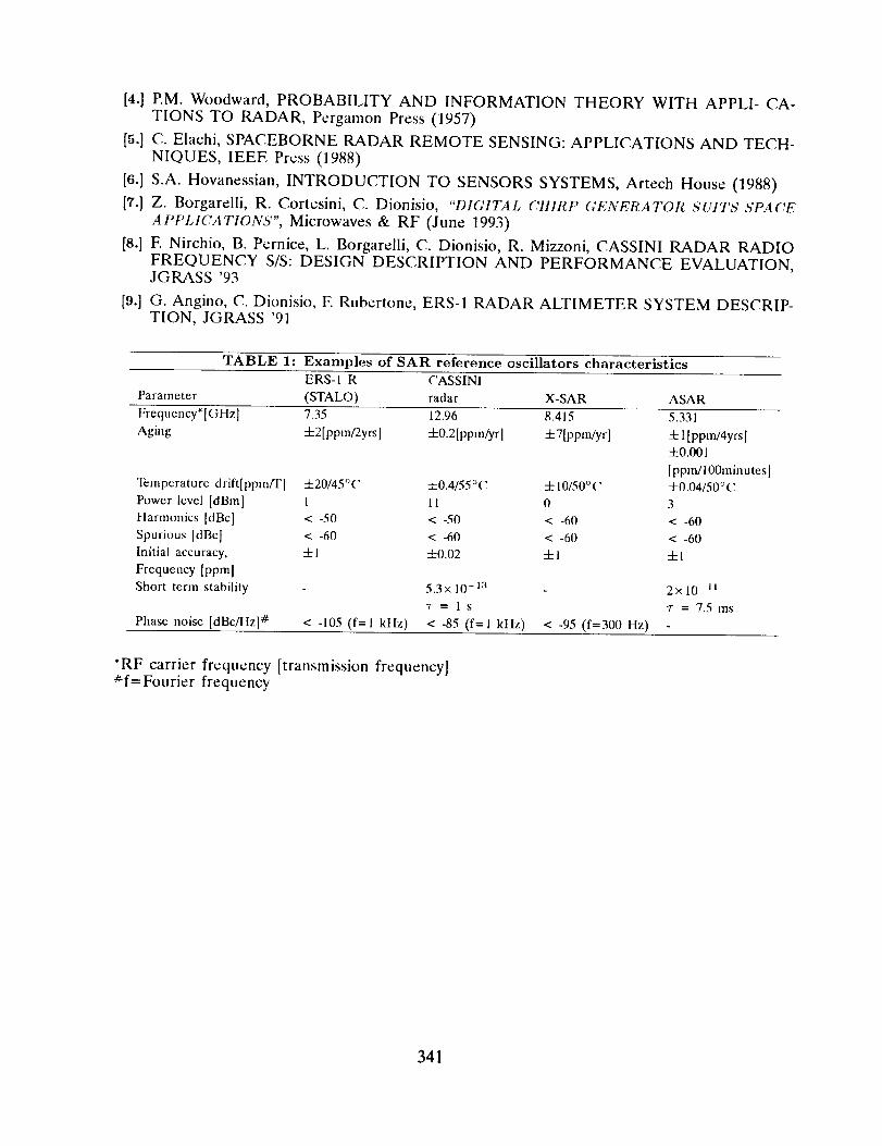
[4.] RM. Woodward,PROBABILITY AND INFORMATION THEORY WITH APPLI- CA-TIONS TO RADAR, PergamonPress(1957)

[5.] C. Elachi,SPACEBORNERADAR REMOTE SENSING:APPLICATIONSAND TECH-NIQUES, IEEE Press(1988)

[6.] S.A. Hovanessian,INTRODUCTION TO SENSORSSYSTEMS,Artech House(1988)[1.] Z. Borgarelli, R. Cortes±n±,C. Dionisio, "DIGITAL CHIRP GENERATOR SUITS 5;PA('E

APPLICATIONS", Microwaves & RF (June 1993)

[8.] E Nirchio, B. Pernice, L. Borgarelli, C. Dionisio, R. Mizzoni, CASSINI RADAR RADIOFREQUENCY S/S: DESIGN DESCRIPTION AND PERFORMANCE EVALUATION,JGRASS '93

[9.] G. Angino, C. Dionisio, E Rubertone, ERS-1 RADAR ALTIMETER SYSTEM DESCRIP-TION, JGRASS '91

TABLE 1: Examples of SAR reference oscillators characteristics

ERS-I R CASSIN1

Parameter (STALO) radar X-SAR ASAR

Frequency*[GHz] 7.35 12.96 8.415

Aging +2[ppm/2yrs] +0.2[pplnPyr] 271ppm/yr]

"Ibmperature drift[ppm/T] +20/45°(" 20.4/55°C 4-10/50oC

Power level [dBm] 1 11 0

Harmonics [dBc] < -50 < -50 < -60

Spurious [dBc] < -60 < -60 < -60

Initial accuracy, +1 +0.02 + 1

Frequency [ppm]

Short term stability 5.3× l0 -13

_-=ls

Phase noise [dBc/Hz] # < -105 (f=l kHz) < -85 (f=l kHz) < -95 (f=300 Hz)

5.331

21 [ppm/4yrs]

4-0.001

[ppm/lOOmmutes]

20.04/50 ° (,

3

< -60

< -60

+1

*RF carrier frequency [transmission frequency]#f= Fourier freqt, ency

341

TABLE 2: Comparison of parameters relevant to the one-way

synchronization between GPS and a SAR system

Parameter GPS SAR Comments

RF Carrier 1.2, 1.5 GHz l0 GHz _" Ionospheric delays are smaller for higher RF carrier

frequencies

,_ 300 MIlz Available Bandwidth*

1+5 kW Determines the (peak) S/N oil reception*

1000 kin Determines tile S/N oil reception*

Chirped pulse GPS modulation is more efficient in making maximum

use of available bandwidth and link power budget

Orbit Polar (,overage of polar regions for geodesy purposes is

possible with the SAR concept

About 4+ 6 passes SAR in polar orbit does not provide a continuous

coverage

per day

RF Bandwidth + 10 MHz

RF Power _ 10 W

Height 20000 kin

Modulation Spreadspectrum

Inclined

Availability ('ontiuuous

"See eq. (8)

_'Thc sample figure refers to an X-band SAR

342

FIGURE I:SAR Concepts

_A

'-°7/i"',,,,

r Z_T

t_on of motio,t J ll. = c 2co_,b

17 R A

Y 2v_ .:_/1)o.,,,

SAR GEOMETRY AND X-Y RESOLUTION

343

FIGURE 2:Transmitted waveform of a linear FM pulse (chirp)

Amplitude

Ttmc

FIGURE 3:Received waveform of a FM pulse and pulse compression

Arnpl_¢ude Re_e_ed pulse

-I

I Frequency

/2 /

0

Delo_

tt

/1 /z

Amplitude

Yt rr'.e

J tme

[, requertcy

CorrLpresscd pulse

I'

: I

--I _; ....

344

FIGURE 4:Digital Chirp Generator (DCG) block diagram

I I I

(38k4Hl)

r.....21......I IIL

CLC_:K rT.... I--_._ _, I I FI-, .... I..... !

Ix:__ /__, i F......J......

INCO

FIGURE 5:Ground Timing Receiver block diagram

RF

SUBSYSTEM

I NAV & TIME l

r-- MSG

DECODER

PULSE ICOMPRESSION

Frequency Dependent I I,,

Delay I

SAR TIMING RECEIVER BLOCK DIAGRAM

L ...................

× Y Z 1

TIME INTERVAL _.

COUNTER• i

Slop T SIall

fcqw

LO_L_LO_

User (local clocK)

COOldinales

Xu, Y,_. Z

pC

i!

ii

#Clock Offset

At

345/346

N95. 32340

Metafitting:

/

#

Weight Optimization for Least-Squares '

Fitting of PTTI Data

/

R.J. Douglas and J.-S. Boulanger

Time and Frequency Standards Group

Institute for National Measurement Standards

National Research Council of Canada

Ottawa, CANADA K1A 0R6

(613) 993-5186, Fax (613) 952-1394

Abstract

For precise time intercomparisons between a master frequency standard and a slave time scale, wehave found it useful to quantitatively compare different fitting strategies by examining the standard

uncertainty in time or average frequency. It is particularly useful when designing procedures which

use intermittent intercomparisons, with some parameterized fit used to interpolate or extrapolatefrom the calibrating intercomparisons. We use the term "metafitting " for the choices that are made

before a fitting procedure is operationally adapted. We present methods for calculating the standard

uncertainty for general, weighted least-squares fits and a method for optimizing these weights for a

general noise model suitable for many PTTI applications. We present the results of the metafittingof procedures for the use of a regular schedule of (hypothetical) high-accuracy frequency calibration

of a maser time scale. We have identified a cumulative series of improvements that give a significant

reduction of the expected standard uncertainty, compared to the simplest procedure of resettingthe maser synthesizer after each calibration. The recta fitting improvements presented include the

optimum choice of weights for the calibration runs, optimized over a period of a week or 10 days.

Introduction

In preparing to fit precision time comparison data, usually questions concerning "optimal" fitting

strategies have been addressed in a generic rather than in a specific sense. It. is interesting to

examine whether, for specific cases, significant advantages might accrue from customizing the fitting

strategy to the specific pattern of data points and the noise spectrum. In practice, many really

important choices are made before any fit is finalized, and yet are not necessairly optimized as part

of the fitting procedure. (a) A fitting metric and method must be chosen (such as least-squares

fitting). (b) The set of parameterized b_sis functions must be chosen: ha.sis function number and

type (such _s a second order polynomial). (c) An outlier removal method may be adopted (such

as iterative]y discarding a limited number of points having anomalously high residuals). (d) The

relative weighting to 1)e given to each data point must be determined (such as the use of end-point

only linear fits vs unweighted linear ]ea_st-squares fits). (e) A final "consistency of fitr with data

and noise model" parameter should be derived (such as the reduced X 2 for a lea.st-squares fit with

347

known noise). Many of these choices depend in subtle ways on the type of noise encountered, and

here precise time measurements often provide details of the noi_ spectrum which are not trivial to

incorporate into an optimal treatment of (a)-(e). Since the term "fitting" is generally interpreted

a.s referring to the determination of a set of parameters from a particular data set, we use the term

"metafitting" to encompass the optimization of the broader processes such as (a)-(e).

But in what sense is this "metafitting" to be judged? At first sight, there appear to be too many

choices. The fitting might be optimized in an average sense, minimizing some metafitting metric

function that sums over experimental residuals. If the autocorrelation function of the noise is

known (or modeled) it. is possible to calculate and minimize the metric function summing over the,, • ,,expected residuals at unmeasured times. Thus the fitting nfight be optinfized in a local sense,

minimizing a residual at a specific time (open to choice), or it might be optimized to minimize

a residual of the average frequency over a specific interval (each end being open to choice). The

point, points or interval must l)e chosen, and a procedure must be found to estimate the expected

residual(s) at times other than those at which measurements have been taken.

Fortunately, international guidelines [1] now strongly suggest a good quantity to optimize: the

"standard uncertainty", which is the root-mean-square residual of the fit's extrapolation or inter-

polation to a specific point, one not necessairly included in the fit. It is also a good quantity

to optimize in that. a standard method [2](the Wiener-Kolmogoroff theory) exists for any fitting

procedure that uses a linear combination of the data. All least-squares fitting procedures with

linear coefficients can be handled explicitly in this way [5]. For the purposes of time and frequency

metrology, metafitting to minimize the standard uncertainty is a good choice - but it might not

be as good a choice in other applications (where, for example it might be more appropriate to try

minimizing the occurrence of outlier events having disasterous consequences). For frequency or

time interval metrology, the standard uncertainty in the average frequency over an interval makes

an even more attractive discriminant for metafitting.

The power law noise models appropriate for PTTI phase comparisons ('an have low frequency

divergences that appear to be worrying to some purists who wish to assure strict stationarity of

any process before developing its formalism. In the development of computable forms [3],[5], it is

straightforward to show that the standard uncertainty in the average frequency of a lea.st-squares

fit, is not divergent for most commonly encountered power law noise spectra, with the exception of

random walk frequency noise. However, the real question is more stringent, than simple stationarity:

have we enough long-term data on the system being modeled to obtain results which converge?

We believe that this type of question can be rigorously handled by imposing a low-frequency cutoff

(and thus ensuring a formal stationarity), and then verifying not merely that any results extracted

from tim model converge as the low frequency limit approaches zero - but also that the results have

converged to the desired degree before the low frequency limit is sampling Fourier components of

the noise which have not, been measured.

Choosing Weights in Weighted Least-Squares Fits

We present here a general strategy for evaluating and optimizing distributions of weights in a

weighted lea.st-squares fit to phase data. We will concentrate on optimizing fitting that compares the

348

fl'equency of a continuously operated oscillator with a frequency standard (perhaps intermittently

operated), for the purposes of frequency calibration. The strategy is based upon the analyticexpressions for the standard uncertainty in frequency, generally extrapolated over a wider interval

than the calibration interval, where a dense set of high-precision phase comparisons would norInally

be available. A noise model is assumed which has wide applicability to a broad range of frequency

standards. The degree of frequency control will be evaluatable for any set of weights in a weightedleast-squares fit that. is lineal' in tile fitting coefficients (but fully general in the choice of basisfunctions).

As our metafitting metric we choose the standard uncertainty in the average frequency, evaluated

over a general interval which could be considerably displ_ed from the fitting interval. This is

the most appropriate metric for frequency metrology applications, since the standard uncertainty

is now the internationally recommended [1] way of specifying calibration uncertainty. With ourprocedures the standard uncertainty in average frequency can be evaluated for a broad class of

noise models, for any set of fitting points, for any extrapolation or interpolation interval, for any

linear combination of arbitrary basis functions, and for any least-squares weighting. In particular,

in any of the above cases our procedure can evaluate the standard uncertainty the equal-weight

procedure (advocated for its robustness) to the end-point procedure (advocated for it.s "optimum"

estimate of fl'equency for some pure (:lasses of noise), _s well _s any intermediate case with higher

weights near the end-points of the calibration interval. The procedure permits the evaluation of the

trade-off of uncertainty for other procedures which are percieved as being more robust. As is shown

below, even with large data sets, in some cases it appears to be feasible to choose the optimum

set. of weights which minimize the standard uncertainty in average frequency for the interval beingconsidered.

Noise Model

The noise inodel x,,(t) is the modeled phase difference between the master frequency standard

and the standard being calibrated. The noise model is taken as being the sum of a deterministic

part. (which could include a phase off.set, frequency offset and frequency drift) and a random noise

part, xo(t). The random noise includes the "full" noise model that is usually used in discussions of

frequency standard stability [9]: a sum of five noise processes, each normally distributed about the

mean (but with variances which depend on the time sampled in different ways) that have spectral

densities of phase noise (S_(f)) that are power laws which range from flat to increasingly divergent

at low frequencies..Ex_si_lg the five terms in terins of the spectral density of the mean-squareof the fluctuations m _ (,or yo(t)) at a frequency f, Sy(f), each noise term is described by an

amplitude h,_ which is taken to be independent of an), time translations (stationarity and random

phase approximations). The stun includes _ = 2, white phase noise in x; (_ = 1, flicker (l/f) noise

in x; (t = 0, white frequency noise and random walk phase noise; a = -1, flicker frequency noise;

and (t = -2, random walk frequency noise. A low-frequency cutoff ft and an upper frequency cutoff

fh. The spectral density of the mean-square fluctuations in xo(t) is Sx(f), and for this noise model

349

2 2 h,_f(,.-_) (1)and S.(f)= E (2rr)2Sy(f) = E h_f"

Ot_--2

For a given noise model of this type, the standard uncertainty of tile fit at any given time can be

calculated from the autocorrelation function (x0(t)x0(t + r)). It is divergent for four of our five

types of noise unless a low-frequency cutoff is applied, and even then can challenge the accurax:.v

and dynamic range capacities of classical computing. Analytic expressions for this autocorrelation

function exist for each type of noise [5], and modern arbitrary-I )recisi°n c()mputer languages m'e

able to cope directly with the autocorrelation function.

In our analysis of the uncertainty a._soc:iated with any useful least-squares tit, we expect no di-

vergences to infinity ill the slandard uncertainty, and so the combinations of the autocorrelation

functions ln/lsl have their divergent parts cancel, with the fitting itself acting as low-frequency cut-

off. In considering the standard Ulu.ertainty of average frequency from a lea_st-squares fit, we have

found it helpful to use analytic expressions [5], [4], [3] fur the less divergent, general two-interval

covarialwe of the random noise model, tha_ is the covariance of the time-scale departure ow_'r the

time interval [t_, t2] with the tinle-scale departure over the time interval [ta, t4]:

S = - x0(t,)l [x0(t4) - m0(t3)])

= (yo(t') at'• 1 3

=

(e)

where @[,,.r..]g[,:,,,,]) is the general c,,variance of the average frequency: a generalization of the

tw_-sample variance of the average frequency. The generalization includes the possibility of an

overlap of the intervals (as well as the possibility of a "dead lime" between the intervals), and

incorporates the possibility of considering the frequency average over two time intervals of different

duration. Just as for the two-sample variance of Y, and fur the autocorrelation function of x(t), the

covarian,:e separates into the live terms of the noise model.

Analytic forms for the five terms of the autocorrelation function of x(l) and for the tive terms

of the general cross-correlation of O are given in references [5], [4] and [3], derived with only the

usual a._sumptions about high and low frequency limits to the noise bandwidth. The references also

contain some comments on practical methods for colnl)uting values using these forms.

Weighted Least-Squares Fits

Weighted least-squares fitting chooses the 7_ linear coefficients dl of the z_ basis functions gl(t),

to re'rive at a function xv(t) which will be used for interl)olation or extrapolation. In frequency

slandards work, we would usually tit a phase ofl_,;et, a frequency off, el, and sometinms a drift, rate

and higher terms such _u_daily or seasonal fluctuations.

350

Tt

xp(t) = d. _(t) = d_ + d2t + d# 2 + E dtgl(t).1=4

(a)

The coefficient vector d-is chosen to nfinimize the sun, over the N fitting points with phase differencevalues of x(ti) at times t,

j_r

= - d. (4)i = 1

where the weight, Wi is applied to the square of the i tl_ residual. Lea.st-squares fitting is done by

setting the n derivatives of L_ equal to zero, which gives a set of n linear equations which can

be solved for the n fitting coefficients of _ Gd = ._', where 131 is an n x n matrix with elementsC'q,. N

---_ _Z=I Wigq(t,:)g_(ti), and ._'is an n-dimensional vector with elements .% = _,(_ 1 I_Vixo(ti)g_(t,).

For the purposes of modelling the standard uncertainty, we use :c0(/i) to model x(ti), since it can be

shown [5] that any general offset in phase, offset in fl'equency or a linear frequency drift is exactlyabsorbed by the fit..

Metafitting with Time Uncertainty Metric

One candidate metric for judging weighted least-squares fits is the standard uncertainty in time,

determined at a specific time t, relative to the set of filling points {I7.}. We can exl)licitly calculate

the effects of the weighted least-s(luaros fit reacting to the noise model for this time t: we are not

restricted to studying the variance at the fitting points. The expected variance in at.(/) from the fit,

d..q'(t) can be calculated in terms ,)t' the autocorrelation functi,m te.ft < xo(ti.)xo(ti),

N N

:i:0 .i::o

w|lere Do(l) = 1 and I)i(l) = [,'VIE n v TM :o_-17--1 z_,_=l_ )q_g,.(t,:)gq(t). For the standard noise model,

the autocorrelation function (Xo(t)xo(t)) can be evaluated analytically [5], although 1he result-

ing expressions can challenge the dynamic range of c(mventional computing. The square root of

this variance in x(t) would be the formal metric. The minimization problem, for optimizing this

metric with respect to the weights W,, looks intractable, 1)ut for cases of most interest it (:an 1)e

substantially simplified in the same way as is described below for tile frequency uncertainty metric.

Variants of this L2 metafitting lnetric are also possible, sulnlning variances over multiple tesl times.

Otiler metafitting metrics of the L:norm (Holder norm) class, could also be constructed. The

rain-max (lira p _ oo) norm would minimize the maximum exl)ected time deviation mnongst the

test times. Metafitting with the p = 1 metric would (for this (:lass of metrics) give the most leeway

in allowing a small number of test points to have large variances. All these metafitting variants are

351

substantially more intricate to use, and do not readily yield the major computational simplifications

which carl I)e found for the single-point L2 metric.

The method outlined above does not bring airy great new insights into optimal ways of combining

equivalent clocks, nor for the optimal use of continuously operated primary standards, however when

a secondary time scale is to track a primary time scale where only intermittent intercomparisons

are available, an optimal choice could be made in terms of the noise processes known to be present.

Metafitting with Frequency Uncertainty Metric

For precise time interval work, where the average frequency is the chief quantity of interest, we

wish to minimize the standard uncertainty in average frequency over an interval [t, t + r], caused

by the noise model as filtered by the weighted least-squares fitting procedure to the points {ti}.

Although the noise model is independent of time translations, clearly the standard uncertainty in

average frequency, %, would be expe(:ed to depend on the offset of t from {ti}, as well as the

interval breadth r. It is defined by

T T

(6)

N+1 tandt i N+I =t+r.We note that. {xo(t+T)--Xo(t)} = E.j=I [xo(tj)--Xo(t._-l)], if we define t.#:0 = .-

Although it. might be convenient to envisage the set of {th} as an ordered set with t_ > t i-l,

it, is not necessary to do so. Ordering the fitting points does not detract from the generality in

any way, but we do not wish to restrict the values of t or t + r. We would like to re-express the

d. {g(t + r)- g(t)} a_ a sum over only differences of the form xo(ti) -xo(t._). We note that we cani

expand xo(ti.) = xo(t.1) + E i=2lxo(t.i) - zo(t.i-1)}, so that d. {j(t + r) - if(t)} is equal to

a -_ __,w:o(t_). {g(t+ _) - ._(t)}=i 1

N i. n n

_2 _<_t_0(tO- _0(t,__)}_ _(a-_)_o_(t,){o_( t_+ _1- 0_(_)}1 j=2 q=l r=l

N n

i=1 q=l r=l

(r)

and the last term, nmltiplying xo(tl), can be shown to be equal to zero. To show this, it is sufficientIV , ,to show that _i=1 W, ff(ti) G-l_(t) is independent of t, or that _N 1 Wig(ti) G-1 is equal to the

vector [1,0,0,...0]. We observe that, from our definition of G and since 91 = l, G[1,O,O, ...0] =

_7,N1 Wi_(ti), and premultiplying by G -1 completes this proof, provided only that gl is a constant.

Thus @(t, r)r 2 is equal to

352

N+I

< [_ {_o(t.j)- xo(t.__l)}j=l

N i n n

-_ m Elx0(t_) - x0(t,_,)} _ _(G-')qT0r(t_){9_(t + 1-1- 9_(t)}]2 >=i=l j=2 q--1 v=l

N n

< [{xo(tN+,) -- x0(t0)} -- _ m {x0(t,:) -- xo(ti-1)} £ _-_(G-l)qrgT(tOlgz(t + 1-) -- gq(t)}]2i=1 q=l r=l

(s)

>

Collecting the expressions with the same difference term {x0(tj) -x0(tj_l)} allows us to write auseful form, namely

N+I

,-,_(t,1-)1-2=< [_ b._(t,1-){_o(tj)- _o(t.j<)}] _j=l

>, (9)

where for 2 < j < N,/)_(t, r) 1 N _ ,_- - = -Ei=.i Wi Eq=l E,=l(G-1)qrgr(ti){gq(t+l")-gq(t)}; D.j=l(t, 1-) =

1 and Dj=N+I (t, 1-) = 1. Multiplying the terms explicitly gives a computable form for the standard

uncertainty in average frequency:

N+I N+I

u_(t, 1-)1-2 = E E D._(t, 1-)[)k(t, 1-) < [xo(tj) - xo(tj-1)][xo(tk) - xo(tk-1)] >.j=l k=l

.0o)

The utility of this form lies in the fact. that it is a sum over functions of the general form of Eq. 2,which are easier to compute for our full noise model.

Metafitting Weights for Large Data Sets

For a given noise model (defined by the 5 parameters {h_} used to define Sy(f), and a given

distribution of fitting points {tv-}, and for a given interval It, t + r]; the standard uncertainty in

average frequency over the interval can be calculated: Uu(t , 7-). Thus a choice of weights can bedetermined which minimizes Uu(t , 7-), the standard uncertainty due to the effects of the random

noise. For each fitting point "added, another weight must be determined. For small sets of fittingpoints, the nfinimization problem is tractable, but for larger sets the minimization appears much

less straightforward. The weights could be parameterized to reduce the dimensionality of theproblem, at the expense of generality.

The full generality can be retained by largely linearizing the problem. For N fitting points, there

are also N weights to choose. Without loss of generality, the set of weights {Wi} can be normalized:

Y_-_=IW,: = 1. If the partial derivative of G -1 with respect to I,Vk can be constrained to be zero, then

most of the N-dimensional search prot}lem can 1)e linearized, leaving a nonlinear search over at worst

353

[(n(_ + 1)/2) - 1] dimensions. G -1 will be independent of Wk if ea(:h element of G is constrained

to be a constant, (;qr = _._':] W_gq(t_)gr(t_). Since Gq_ = (;,.q, and since normally 91 = 1, there

remain [(_(T_ + 1)/2) - 1] values. These (.onstraint equations are used in the linear solution, and

the opt.inmnl values of (;q,_ can subsequently be found by nonlinear searching techni(lues.

For polynomial fitting, with 7_ basis functions {gk(t) = t k-1 }, the partial derivative of G -1 with

respect to [N - 27_ + 2] W_'s there would be only [2n- 2] dimensions for the non-linear search, and

if the pr()b]em (:an be set u l) symmetrically about the time origin, so that the first moment of the

weights and all odd moments are zero, there would be only [n- 1] non-linear search parameters.

The even moments of the weights (summed over the fitting times {ti}) would then I)e the [n - 1]

non-linear search parameters. If the problem is intrinsically a.symmetric, then there would be

[2n - 2] moments to use as nonlinear search parameters. For extrapolation, it seems (:lear that

there will l)e little likelihood of driving any Wi_ negative, but it remains a concern for the general

case and must I)e guarded against.

('_onsider for example the (-a.,_e of choosing a weighted least-squares fit. of a general quadratic to N

phase comparison data points at a specific set of times {ti}. For a specific noise model described

1)y the coefficients {ha}, we want to choose the weights to minimize the standard uncertainty in

the average frequency over the time interval It, t + _-]. By constraining weights to sum to 1, and

I)y constraining the first, through fourth moments of the weights to be independent of the first

[N -4] weights, we can ensure that G -I is independent of [N -4] weights. By equating to zero the

[N -4] partial derivatives of .u_(t, _-) with respect to Wi we can minimize the standard uncertainty

in average frequency with respect to these [N - 4] weights. The easiest form to differentiate for

this purpose is one like that of Equation 8, which has collected all the terms multiplied by any

weight tV_. Including the constraint equations, we then have N linear equations in the N unknown

weights {W,}, parameterized in the 4 moments remaining to I)e searched. The optimized standard

uncertainty for this set of four moments is evaluated, and a four-parameter search (each set of

moments being optimized by re-solving the N linear equations) this search is tractable by the

simplex method (for example). If the problem is symmetric about some time (symmetry for both

{tT} and [t,t + r]), it can be set up so that the first and third moments are zero, and there would

1)e only two parameters to search.

Choosing weights is simpler for a linear lea,st-squares fit to N phase comparison data points,

taken at a specific set of times {t_}. To metafit the best weights that minimize the standard

uncertainty in the average frequency over the interval [t,, t, + T] for the noise model of interest,

described 1)y the coefficients {h_}, we can again linearize the problem - but with only two search

parameters (the first and second moments of the weights). We define three constraint equations

_N=I W_ = 1, _N= 1 W,t., = M1 and _N_ 1 W3_ = M2. The N partial derivatives, with respect to

the weights, of the standard uncertainty in average frequency over the interval [t, t + v] give a set

of N equations F. I/V = _, where F_,._= (ti - M1)r/(M2 - M 2) < [x0(t,_) - xo(tl)][xo(tj) - x0(tl)] >

and r i =< [x0(t + T) -- XO(I,)][XO(Ii) -- x0(tl)] >. The first column of F is a column of zeros. Three

of thee equations are to be replaced by the three constraint equations: one replacement is for the

most ill-conditioned equation j which has t,.i closest to the centroid of the weights (M1) for this

iteration, the other two replacements are more arbitrary. If the problem is symmetric about some

time (symmetry for both {ti} and It, t + T]), it can be set up so that the first moment is zero, and

there would l)e only one parameter to search.

354

An even simpler case of metafitting is the choice of weights in a simple weighted average, for multiple

calibration runs to minimize the standard uncertainty in the average frequency for a specific period,

arbitrarily placed with respecl to the calibration runs. We consider calibration intervals long enough

to be in the regime where the two end point, method is chosen for each calibration run, with M

such calibration intervals [ti, ti + ri]. l_%r the weighted average of the a4 calibrations, the standard

uncertainty in the average frequency over an interval [t, t + r], u_(t, r) is

"4(t,t,+ ,1 + ,-)-_- _ ,,,{*O,+ ,-,)- xO,,:)}]r i:=1 r,: }" (11)

Assigning a weight of -1 to the interval [t, t + r], defining r0 as being equal to r, Equation 11 canbe rewritten as

A solution for the optimum weighting procedure is relatively easy to find since the minimum value

for u_(t, t + r) is to be found for vah, es of wi satisfying 0 [u?(t t + T)] 0, thatso after takingthe derivative and separating out the i = 0 term

M

E _([x(ti + ri) - x(ti)l[x(tk + rk) - x(tk)])i 1

1= --([x(t + r) - x(t)][x(tk + rk) - x(tk)]).

I-k (la)

We use M - 1 of these equations, and for the ki th equation we use the normalization equationof the weights: _M 1 w, = 1. This gives M simultaneous linear equations in the M unknown

weights. The general interval covariance has analytic forms for our noise model, in terms of the

Z-function [4]. If we define the M x M matrix F: P_,.¢ = 1 for j = 1..M, F_ -_[2-(t_ + r,: - t i )_.,._-- .ri 72

+ Z(t,.i + rj - ti) - Z(ti + ri - t_ - rj) - Z(ti. -/.j)] for i = 2..M and j = 1..M, and define ¢: rl = 1

and "i = fraclrr_g(t + r - t_) + Z(tj + r_ - t) - Z(t + r - t_ - r_) - :Z(t - tj)] for j = 2..M. TheM dimensional weights vector t_ is F -1 • 7_

Applications

For any given potential apl)lication of metafitting weights, we must consider whether metafitting

is more than an interesting ac',utemic exercise: can metafitting find a reduction in the standard

uncertainty which is a significant improvement? Since uncertainties are rarely established to better

355

than 10%, an improvement should be larger than this to be deemed significant. Therefore we have

examined the simplest case, of linear extrapolation, discussed above, and for the five different power-

law noise types we have considered distributions of weights with different moments [6]. We have

examined the expected standard uncertainty for both symmetric extrapolation suited to time-scale

calibration (where post-processing can be used to apply calibrations from the "future") and to time-

a.ssymetric extrapolation suited to real-time applications. For symmetric extrapolation intervals

that are large compared to the calibration run's duration, different common weight distributions

gave similar uncertainties (differing by less than 10%) except for white phase noise. For one-way

extrapolation for times much longer than the calibration run's duration, the uncertainties are even

more similar (less than 2% advantage for end-point fitting over equal weights, except for white

phase and flicker pha_se noise). Thus for many PTTI applications, end-point fitting and equal-

weight fitting give similar standard uncertainties, and the choice should be between the greater

simplicity of the end-point fit and the greater robustness of the equal-weights fitting procedure.

In real-life PTTI work, robustness would often prevail over simplicity. For trying to optinfize

results from multiple calibration runs, simplicity is valuable to us while robustness is not needed

in the model. The optimum processing of a number of calibration runs is expected to be largely

independent of the processing within the run.

The main application which ha.s attracted our attention is the optimal use of hydrogen ina.sers,

calibrated periodically in frequency with intermittently operated cesium fountain frequency stan-

dards [8], [6]. We consider two types of maser operation: free-running and autotuned. We use two

power law models for the maser noise, representing a free-running hydrogen maser (type 1) with

h2 = 2.7 × 10 -24, hi -- 2.9 x 10 -3°, h0 -- 2.9 z 10 -27, h-1 = 2.6 × 10 -31 and h-2 =- 7.2 × 10-36; and an

auto-tuned maser (type 2) with h2 = 6.7× 10 -23, hi = 2.9× 10 -3°, h0 = 2.9× 10 -27, h-1 = 7.2 × 10 -31

and h-2 = 4.9 × 10 -37. NRC has two low-flux masers which would benefit from a metafitting

optimization of the weights within a calibration run of an hour, since there is still solne white phase

noise contribution for this calibration interval. Preliminary analysis suggests that the end-point

procedure is within 10% of the optinmm. For phase data taken every 30 s for an hour, extrapolatedto an interval of a day, the end point method is 1.2% better than the equal-weight linear lerLst

squares fit for our free-running maser model, and ms good for the type 2 maser model. Thus we

('an use the simple two end points procedure to establish the best frequency transfer accuracy for

multiple calibration runs. For this procedure the standard uncertainty for multiple calibration runs

can be calculated more easily than in the general case.

Within the context of end-point fitting from eax=h calibration run there are still metafitting choices

to be made about the way in which the runs are to be used. One possible strategy is a loose lock in

frequency: after a calibration run (an hour in duration, in our example) is complete, the frequency

of the maser is reset (through the synthesizer control, for example), either immediately - or after

some delay. Clearly the lemst delay is best, and we chose this procedure with zero delay _s the

reference procedure as we examine a series of possible improvements.

A slightly better possibility might be to have an output tightly locked in phase to the cesium

fountain during the calibration run, followed by a frequency lock to the fitted frequency of the

calibration run. The phase-lock type of frequency control removes the noise of the m_ser during

the calibration run, giving it an advantage that remains noticeable for extrapolation intervals many

times longer than the calibration interval. However, for extrapolations of an hour-long calibration

356

out to a period of a day or more, there is not a large advantage: 2.3% for the free-running maserand 2.4% for the autotuned maser model.

A more significant advantage comes from allowing postprocessing, as can often be tolerated in time-

scale construction and for frequency intercomparisons. We consider a single calibration interval

tc and calculate the ratio of the standard uncertainty of the average frequency over an interval _-

for the best real-time frequency control to the symmetrically extrapolated time interval v. The

quantitative postprocessing advantage will depend upon the specific processing scheme or schemes

envisaged - the duration and frequency of calibration intervals. The postprocessing advantage isup to a factor of two [6].

A postprocessing advantage of two is really quite significant. To achieve the same improvement

in the nlaser ensemble could be done - by increasing the maser ensemble size by four times. The

postprocessing advantage of greatest interest to us is for T representing extrapolation to the time

interval between calibrations - which we expect would be between 1 day and 1 week. Initial interlab-

oratory frequency intercomparisons between cesium fountains, before regular calibration schedules

can be set up, may require extrapolation times longer than 1 week for minimum uncertainty.

Envisaging multiple frequency calibration runs per week, of either hydrogen maser type with a

cesium fountain having a standard uncertainty of 10-14r-1/2 optimistically 5 per week, at the same

time each working day, what is the best weighting procedure for using these calibrations in an

algorithm to determine the frequency over a given interval? For the week's pattern, postprocessing

extrapolation of each day's results independently, using the frequency from the nearest calibration

interval gives a 77_ improvement in accuracy for the free-running maser, and an iInprovement of2970 for the auto-tuned maser.

We have solved for the optimum weights of the maser calibrations to give the lowest standard

uncertainty in average frequency over one week [6]. The week is best spanned by weighting Monday

and Friday runs more heavily, to account for the weekend gap in calibrations. For the type 1 maser,

the optimum weights follow the spanning times rather closely, and the optimum weights offer only

a 1.170 improvement in average frequency. For a type 2 ma.ser, there is a 4.7% improvement.

If adjacent weeks' calibration runs are also available, and the average frequency over a particular

week is re<tuired , the optinmm metafitting includes a small admixture from the preceding and the

following weeks. For a type 1 maser, most of the weight comes from the preceeding Friday and the

following Monday. For an autotuned (type 2) hydrogen maser noise model, the optimum weights

have a slower variation through the weeks, and the three-week optimum has several 70 of the weight

on points that are a full week from the calibration runs of the central week. There is a 1970

improvement to the type 1 maser, and an 1870 improvement for the type 2 maser. The improvements

are summarized in Table I, given with standard uncertainties and cumulative advantages a.s each

improvement is applied. For either maser model, the optimization of weights to apply to each run

over multiple weeks gives about a 20% improvement in accuracy from the equal-weight case. It is

not a large improvement, but it is ahnost free - although it does give additional cross-correlation

between each week's frequency processed in this way. Cascaded with the other advantages discussed

earlier, it results in a factor of 2.2 improvement in the accuracy transferrable with a free-running

(type 1) hydrogen maser; and an improvement of 6470 for the auto-tuned (type 2) maser. For the

free-running maser model, the metafitted optimum standard uncertainty is 6.8 times smaller than

357

method

I f reset to unweighted fit,

II f reset to end points

III phase lock + II

IV daily postprocessed

V metafit 1 week

VI metafit 3 weeks

VII metafit 5 weeks

a,,(rd)

Type 1

uy(Td) Adv.

Gun .

adv.

1.79 x 10 -15 1.00

1.77 x 10 -15 1.2% 1.01

1.73 x 10 -1`5 2.3% 1.04

0.97 x 10 -1`5 77% 1.83

0.97 x 10 1.5 1.1% 1.85

0.81 x 10 -15 19% 2.21

0.81 x 10 -l`5 0% 2.21

5.48 x 10 -15

Type 2 t;um.

Uy (7d) Adv. adv.

1.15 x 10 -1`5 1.00

1.15 × 10 -1`5 0% 1.00

1.12 x 10 -15 2.4% 1.02

0.87 x 10 -15 29% 1.32

0.83 x 10 is 4.7% 1.39

0.70 x 10 -1`5 18% 1.64

0.70 x 10 -1`5 .1% 1.64

1.72 x 10 -15

Tal>le 1: Reduction of standard uncertainty in average frequency at 7 days, for a free-running (tyl)e

l) maser, and an autotuned maser (type 2), when controlled by different methods from five 1-hour

calibrations per week. The % advantage for each inethod is the accuracy improvement over the

previous inethod. The last column gives each method's cumulative advantage over method I, a

synthesizer reset to the least-squares calibration fit. The Allan deviation ay(r = 7d) is also given.

the Allan deviation at. 1 week, and for the type 2 maser it. is 2.5 times smaller than the Allan

deviation at 1 week.

Other interesting strategies are beyond the scope of this work. Longer runs on Monday and Friday

and/or early-Monday and late-Friday calibration runs could be invoked to further improve the

performance. Our methods allow for weight, optimization for any set of calibration runs, and tbr

calculating the resulting standard uncertainty in average frequency.

For some applications, statistical independence of each week, or each 10-day period, may be highly

valued - for example, the clock reports to BIPM each 10 days that are used for determining TAI

(and UT(?) should be independent of each other. Weights for data from the weekly calibration

cycle could be re-optimized for the seven different. 10-day cycles that would exist. The metafitted

optimum weights for the two maser models are shown in Figure 1. For the free-running maser

model, the 70-day standard uncertainty in average frequency is 3.31 x 10 -16 for the combination of

the seven independent optimized 10-day periods, as compared to 3.07 x 10 -16 for the combination

of 10 independent 7-day periods. For the autotuning maser model, the 70 day standard uncertainty

in average frequency is 2.72 x 10 -1° for the combination of the seven independent optiInized 10-day

periods, as compared to 2.62 x 10 -1° for the coml)ination of 10 independent 7-day periods.

Conclusion

Our method for calculating the standard uncertainty for realistic noise models has allowed us to

compare a wide variety of algorithms for treating one particular calibration schedule. We have

metafitted the algorithm in several ways, and have identifed ways to ilnprove the accuracy of the

maser frequency control by 2.2 and 1.64 tiInes. We find that using the 10-day BIPM schedule, with

independent processing of the calibrations for the 10-day periods, the expected asymptote for a

358

single auto-tuned (type 2) maser could reach 1.2× 10 -16 at 1 year. For a flee-running (type 1) ma.ser,

the standard uncertainty at 1 year would be 1.5 x 10 -1° . Thus a flicker floor and accuracy of 10 -16

for the cesium fountain is accessible for periods of a year with current masers carrying tile time

scale. Operating the masers at the stability level of the masers presents a challenge. Transferring

10 -16 frequency accurax:y to a second laboratory also presents a challenge. The reliability of a

cesium fountain which might do this seems to be a major challenge, perhaps comparable to the

challenge of making a cesium fountain with a flicker floor and accuracy of 10 -16. Perhaps the

greatest value of this metafitting procedure is to show the very best performance which might be

extracted fi'om masers represented by these models. If greater accuracy is desired, then different

approaches must be used.

References

[1] Guide to the Expression of Uncertainty in Measurement, International Organization

for Standardization, Geneva, 1993. First edition. (Published in the name of BIPM, IFCC, ISO,

IUPA(:, IUPAP and OIML.)

[2] A. Papoulis, Probability, Random Variables, and Stochastic Processes, McGraw-Hill,

New York, 1965. First edition pp. 400-402. (Omitted from subsequent editions.)

[3] R.J. Douglas and J.-S. Boulanger, Local Oscillator Requirements for 'rimekeeping in

the 10-14r-1/2 era, Proc.eedin9.s. of the 1992 IEEE Frequency Control Symposiutn, pp.

6-26 (1992).

[4] D. Morris, R.J. Dougla_ and J.-S. Boulanger, The Role of the Hydrogen Maser Fre-

quency transfer from Cesium Fountains, Japanese Journal of Applied Physics,33, pp.

1659-1668 (1994).

[5] R. J. Douglas., J.-S. Boulanger and C. Jacques, Accuracy Metrics for Judging "rime

Scale Algorithms, Proc. 25th Annual PTTI Applications and Planning Meeting, pp.

249-266 (1993).

[6] J.-S. Boulanger and R.J. Douglass, Frequency Control of Hydrogen Masers Using High

Accuracy Calibrations, Proceedings of the 199/t IEEE Frequency Control Symposium,

pp. 695-708 (1994).

[7] D.W. Allan, "rime and Frequency (,rime-Domain) Characterization, Estimation, and

Prediction of Precision Clocks and Oscillators, IEEE Trans. Ultrason., Ferroelec.,

Freq. Contr. UFFC-34, pp. 647-654, (1987).

[8] J.-S. Boulanger, D. Morris, R. J. Douglas. and M.-C. Gagn4, Hydrogen Masers and Cesium

Fountains at NRC, in Proc.. 25th Annual PTTI Applications and Planning Meeting,

pp. 345-356 (1993).

[9] J.A. Barnes, A.R. Chi, L.S. C,utler, D.J. Healey, D.B. Leeson, T.E. McGunigal, J.A. Mullen Jr.,

W.L. Smith, R.L. Sydnor, R.C. Vessot and G.M.R. Winkler: Characterization of Fre-

quency Stability, IEEE Trans. hzstrum. Meas. IM-20, pp. 105-120 (1971).

359

Autotuned Maser

Free-running Maser .....................

Optimum Weights for Weekday Calibration

of 10-day Average Frequency

n

4=e

O1oI

4)3:

\

I I

0 2 4 6 8 10 12 14

Time (days)

Figure 1. Optimum weights for combining weekday calibrations that give the minimum standard

uncertainty in the average frequency over a lO-day interval. The calibrating reference standard is taken to be an

ideal one, used for one hour, at the same time every working day. The optimum weights are shown for two flywheel

oscillators: a free-running hydrogen maser model and an auto-tuned maser model. The optimum weights are shown

for a the lO-day period starting on each day of the week.

360

N95- 3234J

Methodologies For Steering Clocks

t

/

i

H. Chadsey, USNO

Abstract

One of the concerns of the PTTI community is the coordination of one time scale with another.

This is accomplished through steering one clock system to another, with a goal of a zero or constant

offset in time and frequency. In order to attain this goal, rate differences are calculated and

allowed for by the steering algorithm. This paper will present several of these different methods

of determining rate differences. Ideally, any change in rate should not cause the of#et to change

sign (overshoot) by any amount, but certainly not by as much as its previous absolute value. The

advantages and disadvantages of each depend on the user's situation.

INTRODUCTION

Although control system theory is not new, it has been more highly developed in some fields

than others. One good example is rocket science and the degree of control theory development

needed for the US Space Shuttle to "catch" the Hubble Space Telescope in December of 1993.

The trick was to meet up with the orbiting unit and grab it. If the control was wrong, the

Shuttle would not reach the unit; pass by it; or, worse, crash into it. This approach to an

offset (in position) is done through the precise firing of rockets. It is a very critical operation

because the rockets have only two states: off and fldl thrust.

The same type of problem faces a laboratory trying to steer the frequency of a clock. The

objective is to maintain a clock at zero (or some other fixed) time offset from some reference

clock. While steering to the desired value, the offset should not be allowed overshoot by any

amount, but most certainly not by the same or more than its previous maximum offset. Animportant difference is that more precise clock control can be obtained because a variable steer

rate algorithm can be determined. This can be done by taking the principles of control theory

as applied in other fields of operation and applying them to the control of clocks.

REASON TO STEER

The need for steering may be understood by looking at what happens when no steering is

attempted. A lab might only monitor the time offset of the clock to some standard periodically

(hourly, daily, weekly, etc.). From these periodic measurements, missing values would be

derived by interpolation, operations would be carried out with no controlling of the clock. For

some applications, especially if they are performed over short periods of time, this is acceptable.However, all clocks have a rate which changes. This is called drift and it is not constant. As

361

it restdt,the clock will bevery far aheador behind andvary in offset amountwhencomparedto the referenceclock, creatingproblemsfor someoperations. (SeeFigure 1.)

STEERING METHODS

To correct for the drift of a clock, the most rudimentary of steering methods can be used.

For example, the clock may be closely monitored and allowed to increase the offset value as

compared to the standard. Once the clock has reached a predetermined offset, it may be

time-stepped to a different value. Operations continue by using the varying offset values and

interpolating between them as needed. This is much like the example of the Space Shuttle

cited earlier, where the space craft is allowed to drift, controlled through the use of varying-

length, full-throttle corrective actions. In the controlling of cesium clocks with this method,there are two major potential problems. First, operations can be disrupted when the clock

is time-stepped. This can in some cases be avoided by performing the steps at times when

the clock is not being used for operations. When the clock is adjusted, very close monitoring

must be performed and methods developed to determine values of offset during the stepping

procedure. Second, cesiums and many other types of clocks can have their characteristics

changed when they are time-stepped. Cesium clocks have been known to change their drift

rate when adjustments of any type are made to them. Again, it depends on how the clocks

are being used whether this will have an adverse effect on operations. (See Figure 2.)

We turn now from the manipulation of the clock to controlling of the output from the clock.

Timing is controlled, not by adjusting the clock itself, bt,t through adjustment of its output with

a phase microstepper or similar device.

The most efficient and drastic of these steering adjustments is commonly referred to as the

"Bang-Bang" mode of operation. The crudest form is the two-stage steering algorithm. This is

the method currently employed by the GPS Master Control Station to control GPS time. This

methodology lets the clock(s) drift at its natural rate until a predetermined offset is reached. At

that time, a frequency change is made to the output (using a phase microstepper, or adjustment

of the clock, etc.). The new drift rate of the ot, tput is in the opposite direction and at a greaterrate than the natural drift of the clock. This new rate is kept until the clock reaches another

predetermined offset value, when the rate is again changed back to its first value. These ratesare ct, rrently +1.0 × 1--19 seconds per second squared for the GPS system. As a result of this

two value steering, the clock oscillates between the extreme offset values. Because the natural

rate of the clock is in only one direction, the "wave" is asymmetric. (See Figure 3.)

The next step in complexity is the three-stage steering algorithm. Here, one has the additionalstate of a zero rate of steer to the system. The theory is that while the clock offset is within

a narrow range of offset, a zero rate of steer is employed by the system. When the offset

is outside this narrow range, the upper or lower steer rate is employed to move the clock to

within the narrow offset range when the zero rate is again used. While this is very easy to

perform programmatically, it still does not correct for the natural rate of the clock. It can also

prodt,ce a wave pattern which may not be stable enough for the operational use of the clock

output. (See Figure 4.)

362

Theprevioussteeringmethodsusea fixed,predeterminedrate of adjustment.Wenextconsiderthe possibilitiesof enhancementto a systemwhen a variablerate adjustmentis implemented.First,when the rate is not fixed,wewill disct,sshow it is determined.Second,wewill seehowthe rate correction is applied.

Oneof the first conclusionsis that the clock cannow be adjustedfor its natural drift. We nolonger have to hassle with an asymmetric wave of offsets. But how can the natural drift ratebe determined?

One method would be to subtract the first data point collected after the last rate change was

applied from the last data point collected and divide by the number of days in the interval

between them. This would result in a rate per day which can easily be t,sed to calculate an

adjustment. This method, however, does have a potentially large fault. If the data are noisy,

the rate determined could be of the wrong magnitude and/or sign.

A second method would be to take an average of the differences between st, ccessive days of

data. This would reduce the likelihood of problems. For a well-behaved system, the taking

of successive differences will allow one to construct where the next data point will lie. As a

rest,It, a rate change can be determined and tested before it is applied to the system. The

problems here are that, depending on the precision of measurement and control desired, the

clock system may not be a well-behaved system; large amounts of data are reqtnired which are

not always awdlable; and this method does not react well to sudden change, such as a clockjump.

A third method would be to perform some type of data analysis on the data points in order

to find the slope of the values. A system of tracking the rate of change of a moving average

or linear line fitting with slope determination over short time periods does very well. It is

improved when, on larger data sets, a data filter is used to remove outlying points. After some

testing, I chose the linear fit method because of its more direct approach, its flexibility to filter

outlying points, and the fact that "one cannot design a filter better than the optimum linearfilter".

Now that we have a way of determining the natural drift of the clock, we can use that to

help in controlling it. This leads to a methodology I will refer to as graduated steering. It

is graduated because the rate of correction applied is no longer fixed, but varies according to

some algorithm. Because we can determine the natural drift of the clock by one of the methods

previously discussed, it follows that we should use that as a starting point for the amount ofthe change.

For example, if the rate of the clock was found to be positive 30 nanoseconds per day, then we

can apply a rate of -30 nanoseconds per day by use of a phase microstepper. The result would

be a clock with a zero rate of change as compared to the reference standard. (The change can

also be an adjustment of the C-field, but a phase microstepper allows for finer adjustments.)

Now that we have created a clock with a zero drift, we must get a zero offset to the reference

clock in order for our operational requirements to be met. This could be done by time

stepping ("banging") it back to zero. This would require the calculation and manual operation

of the time step. It would also mean that our operation could be disrupted by the time

363

d

4

step. The long-term complication would be that if the natural rate of change for the clockwas not determined exactly, after a period of time the procedure would have to be repeated.

This requires constant monitoring of the system, training of personnel in how to make thecorrections, and ascertaining that the corrections are made when they are needed.

The correction to a zero (or near zero) offset can be performed by modifying the rate

determination program to also add a small amount to that required to achieve zero drift. But,how should this additional amount be determined? A method that was used at USNO based

the additional amount on the clock drift. This was found to lead to some undesired effects.

Using the offset value as a factor for additional calculation provides much better control ofthe clock. The idea of steering back to a zero offset should be based not only on the rate

at which one is moving toward or away from it, but also on the present offset value. If, for

instance, one's clock has a rate of 50 nanoseconds per day and the current offset is zero, onewould then introduce a rate change of -50 nanoseconds per day to achieve zero offset. On the

other hand, if one's clock has a rate of 50 nanoseconds per day and the present offset vahle

is 100 nanoseconds, one would introduce a rate change of -50 nanoseconds per day to correct

for the rate of the clock plus an additional amount to get back to zero offset. The additional

amount could be the present offset value divided by some damping factor, say 4. In this case,

the offset would be zero in 4 days time and another rate correction introduced to flatten the

rate of the clock. This method of simple graduated steering will correct for the natural drift

of the clock and if the clock is offset from a standard reference, it will adjust it back to zero

offset. The USNO Master Clock is steered in a similar fashion.

Under ideal circumstances, this simple graduated steering method works fairly well. The

complication arises when one is unable to make one or more of the rate corrections. This

can be caused by the failure of one computer to instruct another controlling the microstepper

to make a change (e.g. because of a faulty phone connection), by computer or microstepper

failure, or, if the operation is performed manually, by the absence of required personnel. The

magnitude of this error can be lessened if a damping factor is used or if the one in use is

increased.

PRESENT USNO STEERING METHOD

The present USNO method of steering remote clocks has developed into a very sophisticated

process that is totally computer-controlled. Operator intervention is needed only in case of

equipment failures or other extraordinary events (e.g. clock jumps or clock replacement). The

process begins by a program determining the offset of the remote clock from the USNO Master

Clock using GPS. This can be done using one of several methods. USNO currently uses the

48-hour running linear-fit melting-pot method. Once the offset for a series of days has been

determined, the steering rate determination program begins to work.

The program to determine an adjustment to the phase microstepper performs several testsbefore the calculation is actually performed. The first test is to determine whether or not a

steer correction is permissible. There is a big danger in calculating rate changes using data

that contains a mix of data from before and after implementation of the last rate correction.

Calculation using mixed data can lead to the steering process causing the clock offset values

364

to oscillatein a veryextrememanner. (SeeFigure 5.) Becauseof this dangerand the useatUSNO of the two-day fit methodof GPSdataprocessing,the steerrate determinationdoesnot useanyoffsetvaluestwo daysfollowingthe implementationof the lastcorrection.

The next test is to makesure that there are enough data to determinean accuraterate ofthe remoteclock. This reqt,iresat leasttwo daysof data. The more datacollected,the moreaccuratethe determinationwill be. However, if too many daysare used,problemssuchasfast reaction to clock jumps and clock replacementwill be created. So, when possible,theminimum amountof daysbetweensteersis used.

As a result of the these first two tests performed by the program, rate changes to the remotelycontrolled clocks occur no sooner than once every four days. Combination of the avoidance of

mixed data and use of sufficient data points can improve clock stability by a factor of ten.

The actual rate change is then determined. From the above tests and predictions of the offset,

it is easy to determine whether the clock is moving toward or away from zero offset and whether

the offset changed sign during the time between the last rate correction and the present or

will change sign before the time of the next rate correction. Programmatically, this creates afour-state test switch:

1. All collected and predicted values are of the same sign and the trend is toward a zero

offset. In this case, the steer rate change would be the predicted value divided by the

damping factor and again divided by the number of days between steer rate changes. Thisdouble division prevents overcorrection of the clock.

2. All collected and predicted values are of the same sign and the trend is away from a

zero offset. In this case, the rate change would be the rate of the clock away from zero

to flatten the clock rate ph, s an additional amount to direct the clock back toward zero.

This additional amount would be the predicted value divided by the damping factor. The

nomber of days between steers is NOT used in the divisor, as this would not cause the

clock to turn around its direction of offset travel. Overcorrection is kept to a minimum

because of the time intervals at which events occur. The correction is applied when theclock has already moved further away from zero than the collected data indicate.

3. All collected values are of one sign and the predicted value is of the opposite sign. Inthis case, it was found from the many possible ways it can occt, r that the best correction

is to make the rate change equivalent to the rate of clock, thus zeroing the clock rate.

4. Some of the collected values are of one sign and the rest of the collected values and the

predicted value of the opposite sign. In this case, the rate change would again be the

rate of the clock away from zero to flatten the clock rate, plus an additional amount to

direct the clock back toward zero. This additional amotmt would be the predicted vah,edivided by the damping factor. The number of days between steers is NOT used in the

divisor, as this would not cause the clock to turn around its direction of offset travel.

Overcorrection is kept to a minimum because of the time intervals at which events occur.

The correction is applied when the clock has already moved further away from zero thanthe collected data indicate.

365

The correctionis thenplacedin unitsof nanosecondsrate of changeperday. Another programimplementsthe changein the phasemicrostepperat the remotetmit. The processis completetmtil the nextcorrection is needed.

RESULTS OF STEERING

Figt, res 6 and 7 show the results of the implementation of the present control program for twosites. The clock being controlled in Figure 6 is located in the office area of an Air Force PMEL.

The clock being controlled in Figure 7 is located in a controlled environment chamber. Both

are rising the same program for determining the rate adjustment for the phase microstepper.

CONCLUSION

With some thought and investigation into the control theories t,sed in other fields of operation,

the timing commt,nity can develop programs to provide more acct, rate and precise control oftime references. This can only lead to improvements in operations and an ultimate savings of

money and personnel time. Control of a clock or system of clocks can range from a simple

manual operation concerning the periodic readjustment of a clock to an elaborate compt, ter

program control operation. The compt, ter control program can be as complicated as the

programmer desires .... intuition is at it premium in nonlinear design" and the control of a

clock system in a changing environment is definitely a nonlinear operation. Beyond a certain

point of complexity, the more that is added to a program, the more likely a control error will

occtlr.

366

U8NO minus UN8TEERED CLOCK

(Figure ])n

a -4000no -5000

-7000

-8000

-9000 -_,-,..,.__s-10000

-11000

49000 49100 49200 49300 49400 49500 49600MJD

USNO minus 8TEPPED CLOCK

n8noSeC

o -100o

S

-2000

(Figure 2)

_ _ I I I I

0_ .

N

- _

I I I I

49000

10

i--

O_

-20

I I I I

I I-%,.%

I !

j-

-10 t I I I I I I 1 , , ,

49t O0 49200MJD

REFERENCE minus CLOCK U81NG TWO-STAGE STEERING

(Figure 3)

I I I ,,,._1 I I I I I I I I

0 10 20DAYS

REFERENCE minus CLOCK USING THREE-8TAGE STEERING

(Figure 4)

I I I I I I ..,,,_ I I I I 1f

f

I I I t J -II I I 1

0 10

f

! I I I

2ODAYS

I I I I

30 40

367

n El Ia 200 :nos 100 -

_ ° •

e¢ O=o

-lOO=S

-200 -

n8noseco

s

n

noS

¢0

9

49020

USMO minus MIXED DATA STEERED CLOCK

(Figure 5)

I I I I I I I I I I I I I I I I i i z i

• o. ° - • o•

I •

• " ° •

• •

1

i t i I I I I ! I ! I I I I I I 1 I I I

49030 49040 49050 49060 49070ldJD

U|klO minus STEERED CLOCK IN OFFICE

(Figure 6)

200

100

0

-100

• ••• • "=

• ,,',.. .,=a

• °•, •••• •• •'°_

• * • ..,'.= °

-20049580 49590 49600 49610 49620 49630 49640 49650 49660

HJD

U8NO minu• STEERED GLOGK IN CONTROLLED AREA

(Figure 7)

100m

O=

-100

-200 ===

-300

-400

• •

• • •

49620 49630 49640 49650 49660MJD

368

N95- 32342

THE EFFECTS OF CLOCK ERRORS ON

TIMESCALE STABILITY

2

Lee A. Breakiron

Directorate of Time



Abstract

The weighting scheme for the cesium clocks and hydrogen masers constituting the USNO timingensemble is reexamined from an empirical standpoint of maximizing both frequency accuracy andtimescale uniformity. The utility of a sliding-weight relation between the masers and the cesiums

is reaffirmed, but improvement is found if one incorporates inverse Allan variances for samplingtimes of I2 and 6 hours for the cesiums and masers, respectively, with some dependence on clockmodel.

INTRODUCTION

Maximum timescale stability and efficient use of resources require the proper relative weighting

of data from atomic clocks. This paper represents a continuation in our quest for an optimal

weighting scheme as the U.S. Naval Observatory (USNO) clock ensemble has changed, firstwith the addition of hydrogen masers to our cesium-beam frequency standards and then with

the introduction of the new-model HP5071A cesit, m standards, which are phasing out our

HP5061 standards. The previous study of our weights was based on data from HP5061 cesiums

and a few masersrli. The lower noise of the HP5071A cesiums justifies a reexamination of ourweighting procedures.

Since timescale algorithms are generally designed to optimize frequency stability, clocks are

commonly weighted according to their individual frequency stabilities, as measured by inverse

Allan variances 1/_r_. A previous study, however, found no significant improvement in our

timescale if inverse Allan variances were used rather than equal weights, so the latter have been

retainedr21. The performance of each USNO clock is closely monitored and any change in its

rate precipitates total deweighting until its behavior is again satifactory and its rate accuratelyredetermined. The deweighting is done automatically in the computation of the near-real-time

mean timescale (done every hourly measurement) toward which the Master Clocks are steered;

deweighting is done manually during the repeated postprocessing which ultimately results inthe final timescale.

The incorporation of hydrogen masers, with their different noise characteristics, requires special

treatment of their data. Some labs use a Kalman filter to handle data from such a heterogenous

369

ensemblel31. We have obtained good results from a sliding-weight relation between the masers

and the cesiums that mirrors their respective class average sigma-tau plots, with the sampling

time _-replaced by the time prior to the latest measureme nt[ll. This results in a time dependence

of the weights, requiring recomputation of the entire timescale every hourly time step. The

masers dominate the clock weights in the recent past, but are entirely phased out over a 75-day

period, so only the last 75 days actually need to be recomputed. This zeroing of the maser

weights prevents any drift of the timescale due to the masers, since even though the frequencydrifts of all clocks are determined and removed front the data, some errors in these drift

corrections might otherwise accumulate.

Still, as data collect, reconsideration of the sliding-weight relation might be worthwhile, as

might that of assuming equal weights for the masers among themselves. Also, fitting average

sigma-tau plots to a class of clocks is not a straightforward, and may be a questionable,

procedure, so the approach taken here is to select clocks of homogeneous type for generationof test timescales whose sigma-tau plots may then be meaningfully compared.

THE HP5071A CESIUMS

The new-model HP5071A commercial cesium frequency standards exhibit a significant reduction

in noise level over the older HP5061 models and other cesiums due to improvements in

electronics and careful allowance for environmental effects [41- USNO currently has 50 HP5071A

ccsiums in 13 vaults or environmental chambers available for timescale data acquisition. In

fact, they have been used in the timescale computation since February 1992. A preliminary

scheme weighted an HP5071A cesium equal to 1.5 times that of an HP5061 cesium.

In order to further investigate their weights, twelve of the best HP5071A cesiums were selected

which displayed constant rate and negligible drift over an interval of 200 days (MJD 49137-

49337, when the reference maser changed rate). Fig. 1 is a sigma-tau plot for the twelve

HP5071A cesiums relative to the Sigma-Tau maser NAV5 (in all such plots, a frequency offset

has been removed). Approximating their weights with inverse Allan variances at a sampling

time of 30 days (around the minimum), we find that the weights range over a factor of 3.1.

However, how valid are Allan-wtriance-based weights for these clocks, and what sampling time

should be used? Though the theoretical answer to the latter for our algorithm is one hour, the

true answers to both questions are affected by noise and systematics. In particular, the noise

of our time-interval--counter measurement system is significant at one hour. A proper gauge

of a clock's contribution to a timescale is:

1 1 1 (1)- -

where cr2,(r) is the reduction in variance contributed by clock i, at2w_i(T) is the Allan varianceof the timescale computed including clock i, and a2_o(_ -) is the Allan variance of the timescale

computed without clock i.

This assumes that the clocks involved are not significantly correlated. This has been found to

370

be the casefor USNO clockswhenthe clocksare not disturbedby environmentaland humaninflncnces[2,sl, which are minimized by the enviromental control and maintenance procedures

at USNO; data affected by such disturbances have been rejected from this study, as they arc

from the computation of UTC (USNO). While correlations may seem to be significant whenclock frequency variations are intercompared[Sl, unpublished USNO results indicate that few of

these cannot be explained by the use of a common reference, as has been found by 0thersl61.

The intention was to use these clocks to generate test timescales, and twelve clocks were thought

to be sufficient to produce a stable timcscale, while still being few enough for such a timescale

to show a measurable effect if one of the clocks was omitted. Test timescales were generated forall twelve clocks and every subset of eleven clocks, using equal weights; the clock contributions

were then calculated via Eq. (1). An indication of the best Allan variance to weight by wot|ld

be that which best predicts a clock's contribution to such a timescale. Unfortunately, a scatterplot showed only that an Allan variance for a sampling time of a few hours was better forweighting than one for a few clays.

To better quantify this, a relative error parameter 0 was defined such that:

L(T) (2)

where cr2V,,(T) is the Allan wtriance of clock i. Values of log¢ are plotted vs. logT for all the

cesiums in Fig. 2. Some points are missing because o was not available when the computed

clock contribution was negative, as it occasionally was, due to noise. Averages were not verystable, but the median minimum relative error occurred for a sampling time of 12 hours.

As a check, test timescales were generated for the same interval and clocks, weighting the

clocks by inverse Allan wiriances over a range of sampling times from 1 hour to 30 (lays. The

resulting sigma-tan plots are given in Fig. 3. There is little difference between most of them,

but the worst are the long sampling times, as one would expect. The best sampling time wasaround 12 hours. Variances computed for T -- 12 hours would also reflect well the effects of

any diurnal environmental perturbations. At v = 12 hours, c_2,i(-r) varied over a factor of 2.8and o_,,(T) varied over a factor of 2.0. Consequently, inverse 12-hour Allan variances will beour choice for weighting the HP5071A cesiums.

THE HP5061 CESIUMS

At present, 14 HP5061A cesiums and two HP5061B cesiums in four vaults or environmental

chambers are available for timescale data acquisition. The sigma-tau plots for ten HP5061A

cesiums are given in Fig. 4 for from 80 to 169 (lays of data. A similar analysis was attemptedof the clock contributions as was done for the HP5071A cesiums. Also, each HP5061A clock

was substituted for a member of the HP5071A ensemble, and timcscales were generated andanalyzed for each. In both cases, the HP506 IA data were too noisy to reach reliable conclusions.

Comparing the average 12-hour Allan deviations in Fig. 4 with those in Fig. I gives:

371

(ano71/cr5o61)= 0.795

Comparingthe median12-hourAllan deviationsgives:

(a,_o7t/cr,_o_l) = 0.785

Consequently, we will adopt a weight ratio of:

w._o61/w,_o71 2 2= cr.5o71/Cr5o61= 0.62

for any HP5061 cesium relative to a typical HP5071A cesium.

As a check on whether equal weights should be retained for the HP5061A clocks, test timescales

were generated for 104 days of data (MJD 49233-49337), weighting by inverse Allan variances

for a range of sampling times. The results are presented in Fig. 5. While inverse 1-hour Allanvariances make slightly better weights than those for somewhat longer sampling times, equal

weights yielded significantly better stabilities than did any of the Allan-variance-based weights.

THE MASERS

USNO currently has three SAO masers and ten Sigma-Tau masers in seven vaults or envi-

ronmental chambers available for timescale data acquisition. During a 222-day interval (MJD

49404-49526) of constant drift and variance, four SAO masers (one has since left) and five

Sigma-Tau masers were selected for analysis. Some rate corrections and occasional outlier

rejections were required, but this is done routinely by the timescale algorithm. Some of thesemasers were steered in frequency, so their data were mathematically desteered.

An n-cornered-hat analysis was performed to obtain their absolute Allan deviations, which are

plotted in Figs. 6 (for the SAO masers) and 7 (for the Sigma-Tau masers). (The analytical

method, which produces identical results as the method commonly in use [71, is described in the

Appendix and is due, as far as we know, to Winkler[81.) The curves for the Sigma-Tau masers

differ systematically from those of most of the SAO masers, as might be expected, since theformer are auto-tuned. The average -r of minimum variance is 0.8 days for the SAO masers and

5.9 days for the Sigma-Tau masers. Approximating their weights with inverse Allan variancesat the average -r of their minimum variances, we find that the weights range over a factor of

166 for the SAO masers and 14 for the Sigma-Tau masers. This indicates that the weights of

the two types of masers should be derived separately and that an tipper limit on the weight of

a clock will be necessary (more on this later).

Meaningflfl computations of clock contributions, then, will require unequal weighting. In orderto determine the -r of the Allan variances for such weights, test timescales were generated

for the above interval and masers relative to the masers MC #1 and MC #2, weighting by

372

inverse Allan variances over a range of sampling times. A three-cornered-hat analysis was

then done between each timescale relative to Master Clock (MC) #1, each timescale relative

to MC #2, and the difference MC #1 - MC #2 in order to determine the absolute Allan

variances of each timescale. The sigma-tau curves of these timescales are displayed in Fig. 8.

At smaller sampling times (where the stability of the masers is of most interest to us), 6-hourAllan-variance-based weights are best.

On that basis, 6-hour Allan-variance-weighted timescales were generated for all nine masers

and for every subset of eight. Clock contributions were next computed as they were for the

cesiums. The corresponding values of relative error _ are plotted in Figs. 9 (for the SAO

masers) and 10 (for the Sigma-Tau masers). Again, some of the points are missing due to noise.

The situation is less clear than for the HP5071A cesiums, but the sampling time of the median

minimum relative error is also 6 hours. Hence, we will adopt 6-hour Allan-variance-basedweights for the masers.

THE MASERS RELATIVE TO THE CESIUMS

The rationale behind the sliding-weight scheme relating the masers to the cesiums is that: (1)

it combines the short-term stability of the masers with the long-term stability of the cesiums;

and (2) it retains the systematic frequency acct, racy of the cesiums as an anchor to the final

timescale, while maximizing the relative frequency stability of the timescale in the recent past,

where it used to steer the Master Clocks. A Kalman-filter-based timescale algorithm can

provide (1), but not (2). As noted above, the method requires recomputation of the timescale

every time step, with the consequences that: (1) our timescale only becomes final 75 days in

the past; and (2) UTC (USNO) at any given time may change by a few nanosceonds duringthose 75 days. The latter is logical becat, se, as data accumulate, clock rates and drifts become

more accurately determined, improving one's knowledge of the timescale at any point in thepast.

As mentioned, HP5071A cesiums have been used in the timescale compt, tation since Febrt, ary

1992. A preliminary scheme weighted the HP5071A cesiums and the hydrogen masers asfollows:

wsoTl(t) = 1/[antilog (O.130x 2- 0.137x- 13.959)] 2

Whm(t) = 1/[antilog (0.309z 2 -- 0.037x -- 14.239)] 2

(3)

(4)

where x = log t. - 5.9, z = log t - 5.2, and t is the time difference in seconds prior to the most

recent measurement. At t = 0, the weight was arbitrarily set equal to t = 3600 (not t = -1,as misstated in [1], p. 299).

In order to redetermine these relations using sigma-tau plots of timescales rather than those

of clocks, test timescales were generated for: (1) the four SAO masers; (2) the five Sigma-Tau

masers; and (3) five of the above HP5071A cesiums, all for the above 222-day interval. The

masers were weighted by inverse 6-hour Allan variances and the cesiums by inverse 12-hour

Allan variances. An upper limit of 33% of the total weight was placed on the individual

373

clock weights. Sigma-tau plots were computed for all three timescales. The ratio of the

corresponding Allan variances for each maser timescale and the cesium timescale were takenand fitted with a second-order curve, as shown in Figs. 11 (for the SAO masers) and 12 (for

the Sigma-Tau masers). The equations of these fits are:

WSA()/5071 (t) = [6.1 ± 0.9](log t) 2 - [79 -t- 9](log t) + [257 4- 221

WS.T/_,071(t) = [5.5 ± 1.4](log t) 2 -- [76 ± 14](logt) + [261 ± 34]

(5)

(6)

where t, the time in seconds prior to the latest measurement, has been substituted for -r. The

weights at t = 0 are arbitrarily set equal to those at t = 3600. These relations reach minima

at log t = 6.5 and 6.9, respectively, at which point they can be ramped down to zero by t =

75 days.

As a final test of the new weights, these sliding-weight relations, 6-hour maser weights, and

12-hour cesium weights were used for the same nine masers and nine of the HPS071A cesiums

to generate timescales for the above 222-day interval. A single sigma-tau plot cannot properlycharacterize such a timescale because of the change in short-term stability relative to long-term

stability with time. Since the cesiums dominate after 15 days in the past and it has been

shown that the new weights provide some improvement over the old, the remaining question

is whether the stability in the last 15 days has been enhanced. Accordingly, the interval was

divided into fot, rteen 15-day segments and timescales were generated for each segment, with

t reckoned from the end of each segment. The Allan variances of these timescales were then

averaged and are presented in Fig. 13, where for comparison there have also been plotted the

corresponding averages if one used the old weightsiii and the new weights but with no slidingrelation. As can be seen, the new weights are a significant improvement on the short term

over both the old and to not using the sliding relation at all.

SUMMARY

The proper choice of timescale algorithm and clock weighting scheme depends on the purpose

to which the resulting timescale is to be pi,t. One objective of the USNO timescale is systematic

frequency accuracy of the final timescale coupled with optimal relative stability in the recent

past for the pt, rpose of steering the Master Clocks. Compromise between these two aims is

avoided by use of the sliding-weight relations between the masers and the HP5071A cesiums

given in Eqs. (5) and (6). Adoption of inverse 6-hour Allan-variance weights for the masers

and similar 12-hour weights for the cesiums will further improve UTC (USNO) by introducing

responsiveness of the timescale to the performance of individual clocks beyond that already

provided by careful monitoring and deweighting.

The new weights for tin HP5071A clock i (of n such clocks) and an HP5061 clock j are,

respectively:

374

and

r+lws071,,(t) = .--,,-- -I[2.,> 1

12,l J

(7)

= 0.62 (w 0:l) t)j(0

where o-_2 is the Allan wlriance for T = 12 hours; I.), and D._ are deweighting factors in case of

changes in performance, an uncertain rate, or an upper limit on the weight; and < > denotes

an average over all clocks. The new weight for a maser k (of a total of m such) is:

]v--, I (,.))Z-_ k -:: 1 _,kJ

where a_is the Allan variance for r = 6 hours, D_. is a deweighting factor, and w_,,,/s071 is givenby Eq. (5) or (6). A upper limit on the weight prevents one or more superior clocks from

dominating the timescale, which might lead to jolts of the timescale in the case of clock failure.

The imposition of such a limit detracts from optimality, but is a requirement for reliability,which is another objective of the USNO timescale.

If the weights were based on stability relative to the mean timescale, a correction factor would

have to be added to Eqs. (7), (8), and (9) for the so--called clock-ensemble effect, which would

otherwise bias the timescale toward the best-performing clockslgl. One may also questionvariances based on reference to a timescale whose own stability changes with time. Both

problems may be avoided by referring the clocks to an unweighted, unsteered (or destcered)maser, rather than to the mean timescale.

Whether the adoption of gradual (robust), rather than instantaneous, deweighting woukl be

a significant improvement remains to be tested; our large number of clocks has not made

this a priority. Our short-term measurement noise should be appreciably reduced when our

experimental Erbtec, or its successor the Steintech, system is reliable and capacious enoughto be implemented, at which time the above weighting scheme will need to be reexamined.

Further automation of the postprocessing procedure and more statistically rigorous treatment

of rate and drift determination and rate and drift change detection are planned.

REFERENCES

[1] Breakiron, L. A., "Ti_.em:ah,. algorithm,_ eombi_iTLq ce._'ium clocks a_d hydro qen. ma-

._'er._," Proceedings of the 23rd Annual Precise Time and Time Interval (PTTI) Applications

and Planning Meeting, 3-5 December 1991, Pasadena, California, pp. 297-305.

[2] Breakiron, L. A., "The e.ffe,:t.s of data proce.s._Mg a)td ene.ivon.meT_tal co_ditio_ts: o_ th.e

¢zeeurac!j of the USNO time.s'e(d_. " Proceedings of the 20th Annual Precise Time and

375

Time Interval (PTTI) Applications and Planning Meeting, 29 November-1 December1988,TysonsCorner/Vienna,Virginia, pp. 221-236.

[3] Jacques,C., Boulanger,J.-S., Douglas,R. J., Morris, D., Cundy, S., and Lam, L. E,"T/me scale algorithms for aT_ imhomo9 eneous group of atomic clocks," Proceedings

of the 24th Annual Precise Time and Time Interval (PTTI) Applications and Planning

Meeting, 1-3 December 1992, McLean, Virginia, pp. 399-412.

[4] Kusters, J. A., "A new cesium beam fT.equency standard performance data, " Proceedingsof the 1992 IEEE Frequency Control Symposium, 27-29 May 1992, Hershey, Pennsylvania,

pp. 143-150.

[5] Breakiron, L. A., "The effects of ar_bient conditions on cesium (:lock 7.atcs " Proceedingsof the 19th Annual Precise Time and Time Interval (PTTI) Applications and Planning

Meeting, 1-3 December 1987, Redondo Beach, California, pp. 175-184.

[6] Tavella, P. and Thomas, C., "Repo_'t on correlations in fl.equency changes among clocks

coT_,tT"ibatin9 to TAI, " BIPM Report 91/4, 1991.

[7] Allan, D. W., "Time and fT.equency (time-domain) characterization estimation, and

prediction of precisioTt clocks and oscillators," IEEE Transactions on Ultrasonics, Fer-roelectrics, and Frequency Control, voi. UFFC-34, 1987, pp. 647--654 = NIST Technical

Note 1337, pp. TN121-TN128.

[8] Winkler, G. M. R., 1994, private communication.

[9] Tavella, P., Azoubib, J., and Thomas, C., "Study of the clock-ensemble co_welation in.4 L(;OS usiug _'eal data, " Proceedings of the 5th European Frequency and Time Forum,

12-14 March 1991, Besancon, France, pp. 435-441.

376

APPENDIX

An n-cornered-hat analysis for the individual variances of a set of uncorrelated clocks may beperformed by writing the variance of the difference between the measurements of clocks i andj as the slim of their individual variances:

for all possible pairs of n clocks and then solving these as a system of n (n - 1)/2 simultaneouslinear equations. The matrix equation could be expressed as:

MX=Y

where, for four clocks:

M

] I 0 0

1 0 1 0

1 0 0 1

0 1 1 0

0 0 ] 1

X y

o-23

c_24

a23

a24O-2

34 .

X may then be solved for by multiplying both sides by the Penrose pseudo-inverse of M, whichhere is:

M-l_

0.3_ 0.33 0.3:_ -0.1B -0.16 -0.16

0.33 -0.1{3 -0.16 0.33 0.3.] -0.16

-0.16 O.:',f_ -0.16 0.3.2 -0.16 0.3.]

-0.16 -0.1_ 0.33 -0.16 0.3.3 0.33

As with the standard n-cornered-hat method, the analysis fails if any of the variances solved

for comes out negative. This generally occurs when the clocks are significantly intercorrelated,causing the variances to be underestimated.

377


MARC WEISS (NIST): The result of that equally-weighted scale looks as good as a

differently-weighted scale. It was rather surprising to me because we fot, nd results that are

rather different.

Also, in general, using weights by themselves is really dependent on what algorithm you're

using. And the tau that's used for determining the Allan Variance, cru(_-), the tau should come

out of the algorithm; the algorithm should dictate the tau you use to determine weights. And

using that kind of analysis, we found quite a difference when we used scales that are weighted

differently for different clocks.

LEE A. BREAKIRON (USNO): It depends on exactly how you intend to ttse the time scale

that you generate. We would like the highest systematic accuracy to determine our final time

scale. That's why we phase out the masers, and we want the highest relative accuracy in theshort term to steer our masers too. Yes, it depends what you are going to put the time scale

to as to what tau you would weight by and whether it would make any difference.

MARC A. WEISS (NIST): What do you mean by "accuracy" in that context?

LEE BREAKIRON (USNO): We want the systematic accuracy of the time scale to be

maximizetl, based only on the cesiums. So that's why we phase out the masers.

MARC A. WEISS (NIST): By accuracy, do you mean "frequency accuracy" or accuracy of

time relative to some other scale?

LEE BREAKIRON (USNO): Right. The systematic frequency accuracy.

JUDAH LEVINE (NIST): I would just like to ask you to clarify your point of your

recompt,tation of the data already submitted to the BIPM. Does that mean that the data in

Circular T are, in fact, amended after the fact?

LEE BREAKIRON (USNO): Slightly.

JUDAH LEVINE (NIST): Is that amendment published subsequently? What I am saying

is that if I look at Circular T and I copy a number down -- I'm trying to understand how it

works.

GERNOT M. WINKLER (USNO): Two things. The Circular T values are determined from

the individual clock readings which we st,bmit to the BIPM. They are not changed. These are

measurements which are made against a physical signal, which is the Master Clock; which is

the same which is used to link to other laboratories.

What we are talking about here is the internal time scale which is used to steer the Master

Clock. There is a very long time constant. We have to have something to steer to us. BIPM,

of course, in a last analysis, is to panel for that. But for the day- to-day performance, wehave an internal time scale, and that is the one which changes. Now that is the internal time

scale which, again, has to be differentiated from the coordinated scale. The coordinated scale

has additional frequency changes imposed because of our efforts to stay as close as we can to

BIPM.

378

So the result is, the bottom line is that the Circular T values fl_r the UTC, USNO are notchanged.

CLAUDINE THOMAS (BIPM): Of course, UTC minus UTC USNO Master Clock is not

changed, for sure. But I think that Gernot is speaking about the second page of Circular T

which gives DI minus the individual TA; while what is called TA USNO is A.1 mean from

USNO and for which we do not have the definitive values, as far as I t, nderstood with this thing

with Dr. Breakiron last Friday. We do not have the definitive values; the values pt, blished are

not the definitive values simply because definitive values are obtained 70 days after the fact,while USND wdues are before 70 days.

But it is true, we have not the definitive wdues. Maybe we can change this for the annual

report. But that is something that I didn't know before coming here. But maybe we canchange this.

GERNOT M. WINKLER (USNO): There is another point. And that is that TAI is not

based on thc contributions of the time scales. It is based on the contribution of individualclocks.

CLAUDINE THOMAS (BIPM): Yes, yes, of cot,rse. The independent time scales are not

weighted in TAI. What are weighted is are the independent clocks supposed to be frec-rt,nning.

But it's true that we are also publishing DI mint, s independent local TA on the second page

of Circular T. And I think that Gernot was alh,ding to that partict,lar pt,blication, which has

nothing to do with the first page which is UTC minus local UTCs. Thank you.

LES BREAKIRON (USNO): I thought of a better answer to Dr. Weiss. You have to realize

that this data have been chosen because they are the highest quality that we have. Anti all

things like rate corrections have already been either corrected for or the clock is removed forthat reason.

So when you're dealing with data of that quality, and it's essentially been combed through likethat, I think you would find results closer to ours.

CLAUDINE THOMAS (BIPM): Excuse me. I just want to add a small comment or

question. On one of yot, r transparencies, there is a difference, something like 1 over variance

equals I over wtriance of something else, mint,s I of a variance of something else.

LES BREAKIRON (USNO): Right.

CLAUDINE THOMAS (BIPM): I'm very suspicious of doing differences of wtriances. If

you have differences of one of a variance, it means you are able to do the sum of one of a

wiriance. And this is only possible, of course, if the clocks are independent and if there is no

limit of weight. As soon as you have a limit weight in any time scale, it is no longer true.

That's an argument against TAI, which is very often said and discussed. Thank you.

GERNOT M. WlNKLER (USNO): I think, since that is a planning meeting and require-

ments of great interest, I would like to hear of anyone who would be affected by these changes

of the internal time scale, after the fact. We have been trader the firm impression that itdoesn't affect anyone, because it does not affect TAI, it does not affect the actual differences

379

whichare reportedon pageone. It only affectsthe differenceof DI minusinternal time scale,whichyou published.

HoweverI would like to hearfrom anyonewho feels that this producesa difficulty.

CLAUDINE THOMAS (BIPM): Of course,the secondpageof Circular T, whichgivesDIminus TAK, is usedonly for laboratorieswhich are givingTA. Of course,this hasabsolutelyno impacton tau and usersof UTC-K, which are published. The use is for you, in fact, toknow it's doing your E.I meanrelativeto TAI. Well, if anyonewants to make the samekindof thing,of course,if he hasnot the last updatedvalues,he is mistaken,of course.

But the primary role of this answeris for the laboratoriesthemselves.

GERNOT M. WlNKLER (USNO): We have to ask ourselves.

CLAUDINE THOMAS (BIPM): Yes. All the users who would liked to be linked for some

reason to A.I mean. Of course, if it only takes Circular T values, they do not have the last of

this. So they may feel mistaken or have a distrust about that.

JUDAH LEVINE (NIST): My comment is that the most important aspect of the Circular T

data is that I understand what it means. Speaking as a user of page two, the most important

characteristic to me is that I understand exactly how those numbers are calculated. And now

that I understand it, I understand it; and before, I didn't tmderstand. And I think that is the

most difficult aspect, is to know what the number actually means or how it was calculated.

RANDY CLARKE (USNO): I'm the one that does it. So just to let you know what you're

facing, I wotdd say that it's probably only a few nss. Because, we send in the reports after 30

days, so the major processing has already been done. So it's very rare that it's over five. If

you're interested in what it is, it's something like five ns.

CLAUDINE THOMAS (BIPM): This can be done so simply in the new report of the BIPM.

Just send me the last values when you have them, and I will publish them in the annual report;

so everyone can get the updates after the fact, and that's all.

380

N95. 32343

Relativistic Theory for Syntonization of Clocks

in the Vicinity of the Earth

£ -_ 9

/

P. Woli <2 and G. Petit 1

1Bureau International des Poids et Mesures,

Pavillon de Breteuil, 92312 S_vres CEDEX, France

2Queen Mary and Westfield College, School of Mathematical Sciences,

Mile End Road, London E1 4NS, Great Britain

Abstract

A well known prediction of Einstein's general theory of relativity states that two ideal clocks

that move with a relative velocity, and are submitted to different gravitational fields will, in general,be observed to run at different rates. Similarly the rate of a clock with respect to the coordinate

time of some spacetime reference system is dependent on the velocity of the clock in that reference

system and on the gravitational fields it is submitted to. For the syntonization of clocks and the

realization of coordinate times (like TAI) this rate shift has to be taken into account at an accuracylevel which should be below the frequency stability of the clocks in question, i.e. all terms that

are larger than the instability of the clocks should be corrected for. We present a theory for the

calculation of the relativistic rate shift for clocks in the vicinity of the Earth, including all terms

larger than one part in 101_. This, together with previous work on clock synchroniToation (Petit &Wolf 1993, 1994), amounts to a complete relativistic theory for the reali_ation of coordinate time

scales at picosecond synchronization and 10 -1_ syntonization accuracy, which should be suJyicientto accomodate future developments in time transfer and clock technology.

1. Introduction

When t, sing the concept of syntonization in a relativistic context certain ambiguities might

appear which can lead to confilsion and misunderstanding. It is therefore essential to first

clarify the different meanings of the expression as used in time metrology within a relativisticframework.

Consider first the case where the relative rate of two distant clocks A and B is measured

directly i.e. the frequencies of two signals coming from A and B respectively are compared by

some observer 0. Taking the case where the observer is in the immediate vicinity of B and atrest with respect to B the measured relative rate is predicted as;

(drA/drB) - 0 = 1 + [(U B - UA) _ v2/2]/c 2 + 0(c-4) (1)

in the first post-Newtonian approximation where (dvA/drB)O is the relative rate of the two

clocks as observed by 0, U is the total gravitational potential at the location of the clock, v is

381

the relative speed of the two clocks and c is the speed of light in vacuum. Note that this result

is completely dependent on the observer 0. If, for example, 0 was in the immediate vicinityof A and tit rest with respect to A the term in v _'_ would change sign. Note also that (1)

is independent of any reference frame or coordinate system. It is a coordinate independent,

measurable quantity.

For the realization of coordinate time scales (like TAI) it is necessary to syntonize clocks with

respect to the coordinate time in question, i.e. to determine the rate of a clock A with

respect to an ideal coordinate time of some space-time reference frame. For example, using

a geocentric non-rotating frame with TCG as coordinate time (as defined by the IAU /(1991))

we obtain, again in the first post-Newtonian approximation;

dT4/dTC(; = 1 - [l"(w) + v'212]1 c2 + O(c-4) (2)

w the triplet w k.where (c_ ,o, wk) are coordinates in the geocentric frame with representing

The potential at the position of the clock U(w) is the sum of the Earth's potential and tidal

potentials of external bodies, and v = ((dwildT('_(;)(dwi/dTCG))U2 is the coordinate speed ofthe clock in the geocentric, non-rotating frame. Note that this rate depends entirely on the

chosen reference frame. It is a coordinate quantity which cannot be obtained directly from

measurement, but must be calculated theoretically using the definition of the reference frame

in question with the appropriate metric equation.

When using repeated time transfers employing the convention of coordinate synchronization

(Allan & Ashby 1986, Petit & Wolf 1994) for the determination of the relative rate of twoclocks A and B, the resulting rate predicted by theory is simply:

• _'-I (dTAIdTC(;)(dT('(,IdTB)(3) (3)dTA/dl f =

with dr/d7'C(; given in (2). This is a combination of coordinate dependent quantities and notto be confused with the measurable quantity expressed in (1). The former is entirely dependent

on the chosen reference frame and the convention of synchronization while the latter is specific

to the measuring observer 0. They will, in general, (lifter due to, essentially, the difference in

the v'_/c '_ terms. In sections 2 and 3 we will consider the syntonization of clocks with respect tocoordinate times TCG (Geocentric Coordinate Time) and TT (Terrestial Time, the ideal form

of TAI) as defined by the IAU (1991) together with the transformation relating the two. The

aim is to provide expressions in the form of (2) including all terms whose magnitudes exceed

current and near future clock stabilities which are estimated to reach parts in 10 TM, as shown

in Figure I (Maleki 1993).

When determining the relative rate of two distant clocks, one might be interested in time

varying effects only (i.e. effects that influence the observed frequency stability), which, as willbe shown, can be calculated at higher accuracies than constant frequency shifts. They arc

discussed briefly in section 5.

382

2. Syntonization with respect to TCG

Using the metric given in resolution A4 of the IAU (1991) the relation between the propertime of a clock T and TCG can be expressed a:

&-I,LTC'(; = 1 - [U(w) + C_(xe + w) - C'(xe) - ('k(xE)w k + ,_212+ qk]/(: 2 + 0(_ -4) (4)

where coordinates in the barycentric frame are represented by (cT(:14, x k) with x denoting

the triplet x k and the subscript E referring to the Earth's center of mass. liE(w) and C_(x)

are the Newtonian gravitational potentials of the Earth and of external masses respectively,

v = ((dwi/dT(;(;)(dwi/dT(,,(;))½, the coordinate speed of the clock in the geocentric, non-

rotating frame and Qk is the correction for the non-geodesic barycentric motion of the Earth.

We find that in the vicinity of the Earth the term in Q and terms of order (?,-4 (given explicitlyin Brumberg & Kopejkin 1990 and Kopejkin 1988) amount to a few parts in 10" or less. This

implies that the specification of coordinate conditions (harmonic, standard post-Newtonian

etc .... ) and the state of rotation of the frame (kinematically or dynamically non-rotating) isnot significant for syntonization at the 10-_8 accuracy level.

All effects that need to be taken into account for the calculation of the remaining terms are

listed in tables la and Ib, together with orders of magnitude and present day uncertainties ofthe associated corrections.

Syntonization with respect to TCG of Earth-bound clocks is limited at the 10 -17 accuracy levelby uncertainties in the determination of the potential of the Earth at the location of the clock.

Hence only effects whose influence on (4) is larger than this limit are considered in Table la.

The gravitational potential of the Earth, Uz(w) can be expressed as a series expansion inspherical harmonics. However, owing to mass irregularities such a series must be considered

divergent at the surface of the Earth (Moritz 1961). Nonetheless, due to the predominantly

ellipsoidal shape of the Earth, one can use the first two terms of this series expansion as a firstapproximation (Allan & Ashby 1986, CCIR 1990, Klioner 1992). Thus:

t';_(w) = c,',,we_,_J_(_-3,:o_ _ 0)/_,,._... (,_)

where (; is the Newtonian gravitational constant, Me is the mass of the Earth, a_, and J2

(,/2 = 1.0826 × 10-3 ) are the equatorial radius and the quadrupole moment coefficient of the

Earth respectively and 0 is the geocentric colatimdc of the point of interest.

Substituting (5) into the second term of (4) gives terms of the order of 7 × 10 -m and 8 x 10 -13respectively for points on the surface of the Earth.

The surface obtained when setting Ue(w)+ (_wsin0)2 = W0 in (5), with _ representing the

angular velocity of rotation of the Earth and W0 the gravitational + centrifugal potential on

the geoid, differs from the ellipsoid of the Earth model by less than 10 m. Hence an estimate

of the accuracy of (5) can be obtained by considering the maximal difference between the

383

geoidand the referenceellipsoidwhichcan amountto _ 100m (Vanicek& Krakiwsky1986).Thereforeexpression(5) for the Earth'sgravitationalpotential shouldnot be usedif accuraciesbetter than one part in 10 TM are required.

On the coast the mean sea level can be determined using a tidal gauge. This level differs

from the geoid by what is known as Sea Surface Topology (SST) which can amount to 4-0.7

m (Torge 1989). The SST can be determined with an accuracy of 0.1 m (Torge 1989) using

oceanographic methods and satellite altimetry which induces an uncertainty of 1 × 10 -17 in

(4). The uncertainty in the knowledge of the potential on the geoid W0, which is of theorder of +lm2/s 2 (Bursa 1992, 1993), contributes another part in 1017. The gravitational and

centrifi,gal potential difference between mean sea level and an arbitrary point far from thecoast can be obtained by geometrical leveling with simultaneous gravimetric measurements.

The accumulated uncertainty when using modern leveling techniques and gravimetry is below

0.5 mm/_ (Kasser 1989) and does therefore not exceed a few centimeters even over large

distances. In many countries leveling networks have been established at accuracies of 1-2

mm/kxfk_ for primary points, the use of which would again induce errors at the centimetric

level.

Therefore the constant part of the total potential at any point on the Earth's surface can be

determined with an accuracy better than 2.5 m2/s 2 using a tidal gauge and good geometrical

leveling. The main contributions to this uncertainty are due to inaccuracies in the determinationof W and the SST. This limits the calculation of the second term in (4) at the level of

2 _ 3 × 1(9 -17 which is the limit for syntonization of clocks with respect to coordinate time

(TCG or TT) on the surface of the Earth.

Uncertainties in the potential model GEM-T3 (Lerch et al. 1992) and the determination of

the satellite orbit (5 cm seems a realistic value) limit the accuracy of syntonization of satellite

clocks at a few parts in 10 TM for low altitudes (semimajor axis < 15000 km). For higher altitudes

the effect of these uncertainties is below the 10 -is level.

Therefore all terms necessary for the syntonization with respect to TCG of clocks on board

high altitude satellites (a > 15000 km) can be calculated to accuracies better than one part in10 TM'

3. Transformation to TT

TCG is related to TT by a relativistic transformations, hence any clock that is syntonized

with respect to TCG can also be syntonized with respect to TT. In this case the accuracy

of syntonization may be limited by the uncertainty in the determination of the parameters

participating in the transformation.

The IAU defined TT as a geocentric coordinate time scale differing from TCG by a constant

rate, the scale unit of TT being chosen so that it agrees with the SI second on the geoid (IAU

1991). TT is an ideal form of the International Atomic Time TAI, apart from a constant offset.

It can be obtained from TCG via the transformation:

384

dTT/dTC(; = 1 - Lg (6)

with L o = Wo/c 2 = 6.9692903 × /O 10 ± 1 x 10 -17.

It follows that at present the accuracy of syntonization with respect to TT is limited at the

10 -17 level due to uncertainties in the determination of the potential on the geoid W0, evenfor clocks on board terrestrial satellites.

This limit is inherent to the definition of TT and can therefore only be improved by a reduction

of the uncertainty in the determination of W0. If highly stable clocks on board terrestrial

satellites are to be used for the realization of TT at accuracies exceeding this limit it might

prove necessary to change the definition. One possibility would be to turn L_ into a definingconstant with a fixed value, which would at the same time provide a relativistic definition of

the geoid (Bjerhammar 1985, Soffel et al. 1988).

4. Time varying effects

For several applications of highly stable clocks, one is interested in the stability of the relative

rate between two clocks, and therefore only time varying effects need to be considered, whichcan be calculated at the 10-18 accuracy level even for clocks on the surface of the Earth. Table

II gives a summary of all such effects estimated to exceed the 10 -18 limit.

Volcanic, coseismic, geodynamic and man-made (e.g. exploitation of oil, gas, geothermal fields)

effects are highly localized and only need to be taken into account at some particular locations.

Polar motion and tidal effects are of periodic nature with essentially diurnal and semi--diurnal

tidal periods, and the Chandler period (430 days) for the movement of the pole. If the clocks

in question are syntonized using repeated time transfers (see (3)) at picosecond accuracy, tidal

terms can be neglected as their short periods prevent their amplitudes in the time domain fromreaching one picosecond (Klioner 1992).

For atmospheric pressure variations of + 10 mbar on a global scale (corresponding to seasonal

changes), the effect on the rate of a clock on the Earth's surface can reach + 2 parts in 1018

with local pressure changes ((anti)cyclones with pressure variations of up to 4- 60 mbar) givingrise to a correction of tip to -t-2.7 × 10 -1_ (Rabbel and Zschau 1985).

5. Conclusion

We have presented a theory for the syntonization of clocks with respect to Geocentric Coordinate

Time (TCG) including all terms greater than 10 -_s for clocks on board satellites at altitudes

exceeding 15000 km. For this ptirpose terms of order c -3 and c -4 in the metric can be

neglected, which implies that the specification of coordinate conditions and the state of rotation

of the reference system is not necessary.

Syntonization with respect to Terrestiai Time (TT), an ideal form of TAI, is limited at the 10 -17

acctiracy level due to the uncertainty in the determination of the potential on the geoid W0

385

inherent to its definition.

For clocks on the Earth's surface syntonization with respect to TCG or TT is limited at an

accuracy of 2 _ 3 × 10 -17 by uncertainties in the determination of the geopotential at the

location of the clock.

We briefly discussed time varying effects that may influence the stability of the relative rate oftwo clocks. These can be calculated at the 10 -1_ accuracy level even for clocks on the Earth's

surface.

At present atomic clocks are approaching stabilities of the order t0 -1_ (Maleki 1993) with

further improvements expected in the near future. For comparisons of these highly stable

clocks over large distances, and their application in experimental relativity, geodesy, geophysics

etc.., a sufficiently accurate relativistic theory for their syntonization, like the one presented in

this paper, seems indispensable.

Together with a previous paper (Petit & Wolf 1994) the results obtained here amount to

a complete relativistic theory for the realization of a geocentric coordinate time scale at a

synchronization and syntonization accuracy of one picosecond and 10 -1S respectively.

References

Allan D.W. & Ashby N., 1986, in: Kovalevsky J., Brumberg V.A. (eds.), Relativity in Celestial

Mechanics and Astronomy. Proceedings of the IAU Symposium No. 114 Leningrad 1985,

Reidel, Dordrecht

Bjerhammar A., 1985, Boll. G6od. 59, p.207

Brumberg V. A. & Kopejkin, 1990, Celestial Mechanics 48, 23-44.

Bursa M. et. al., 1992,, Studia Geoph. et Geod., 36, 101-114.

Bursa M., 1993, I.A.G. Special Commission SCR - Fundamental Constants (SCFC), Circular

No 5.

CCIR, 1990, International Radio Consultative Committee, Reports, Annex to Volume VII,

p.150

IAU, 1991, IAU transactions Vol. XXIB, 1991, Proe. 21st Gen. Assembly Buenos Aires,

Kluwer Acad. Publ., Dordrecht, Boston, London.

Kasser M., 1989, C. R. Acad. Sci. Paris, t. 309, Sdrie 11, p.695

Klioner S.A., 1992, Celestial Mechanics and Dynamical Astronomy 53, p.81

Kopejkin S.M., 1988, Celestial Mechanics 44, 87-115.

Lerch EJ. et al., 1992, NASA Technical Memorandum 104555.

Maleki L., 1993, Proceedings 25th PTTI Meeting 1993, Nasa Conference Publication 3267,

549-560.

386

Moritz H., 1961, Osterreichisch¢ Zeitschrift far Vermessungswesen, v. 49, 11-15

Petit G. & Wolf P., 1993, Proceedings 25th PTTI meeting, 205-215.

Petit G. & Wolf P., 1994, Astronomy and Astrophysics 286, 971-977.

Rabbel W. & Zschau J., 1985, J. Geophysics 56, p.81

Soffei M. et al., 1988, Manuscripta Geodetica 13, p.143

Torge W., 1989, Gravimetry, de Gruyter, Berlin

Vanieek P. & Krakiwsky E., 1986, Geodesy the Concepts, North Holland.

387

Effect Order of magnitude Uncertainty

Earth's grav. pot.

Centrifugal pot.(v2/2/c 2)

Volcanic and coseismic

(highly localised)

External masses (moon, sun)

Solid Earth tides

Ocean tides

7xl0-10 10 It

lxl0 -lz < 10 -is

< 10 16

10-17 ( 10 is

10-17 < 10 -Is

10 -17 ( 10 is

Table la: Effects on syntonization with respect to TUG of clocks on the Earth's surface;

Orders of magnitude and uncertainties of the corrections.

Effect

Earth's grav. pot.

Order of magnitude

< 6x10 t°

Uncertainty

few 10 is (GEM-T3)

< 10 is at a> 10000 km

2nd order Doppler (vz/2/c 2)

External masses: Moon

(at a = 300000 km) Sun

Venus

< 3x10 -10

4xl0-1a )4X10 14

6X10 18

few 10 18 (5 cm orbit

uncertainty)

< 10 is at a> 15000 km

< 10 is at a> 15000 km

( 10 -18

Solid Earth tides )

Ocean tides 10_a < 1018

Polar motion (at low altitudes)

Atmospheric pressure

Table lb: Effects on syntonization with respect to TCG of clocks on board terrestial satellites;

Orders of magnitude and uncertainties of the corrections.

388

Effect Order of magnitude Uncertainty

Volcanic and coseismic

(highly localised)

Geodynamic and man-made

(localised and long-term > 1 year)

External masses (moon, sun)Solid Earth tides

Ocean tides

Polar motion

(long-term - 430 days)

Atmospheric pressure

< 10 a6

< 1016

10 "17

10"17

10 "17

lO-lS

10qs

< 10 _s

< 10qs

< 10 as

< 10 4s

< 10qs

Table II: Time varying effects on the Earth's surface for the determination of the relative

rate of two clocks; Orders of magnitude and uncertainties of the corrections.

-12[" I I I I ICs Fountain-1993 LEGEND:

_ MEASURED

-13 EXPECTED _

Fountain-1995

-14

H-MASER - 1991

a

Z -15.-I

P"ssj

_;3-._..= SCMO - 1995 I / • _ --_

-16 -- ...._'._.... _ • _TRAPPED ....7..._ COMBINED PERFORMANCEION- 1995 _'--..'_.

-18 I I 1 1 "r -..,"-.

,--I

<

0--,I

1 10 10 2 10 3 10 4 10 5 10 6

(seconds)

Fig. 1: Present and expected clock stabilities (from Maleki (1993)).

389


RICHARD KEATING (USNO): I just have a comment. I don't think that the kind of

presentation you just made is particularly useful. I think it's rather misleading. And I would

like to say that because about seven years ago, I fired up an old pendulum clock at the requestof a retired General Electric engineer• And if I had thought along the lines that you've just

presented, I would not have expected to see any effects from, say, a hmar potential. In fact,

the pendulum clock is highly sensitive• I could actually tell where the moon was, simply by the

effect on the pendulum clock.

These are not relativistic effects, true. But they are far more dramatic, much larger, and they

dominate the whole phenomena. So, just to concentrate solely on relativistic effects may be,

I think, highly misleading. So, to talk about 10 -is, which is a tenth of ps per day, when

you actually in reality might have gravitational potential effects, which are the order of ms, I

really think you've got bigger problems to worry about. And I think that this kind of paper is

misleading.

PETER WOLF (BIPM): Okay, that's your opinion. Fine.

R.J. DOUGLAS (NATIONAL RESEARCH COUNCIL OF CANADA): I would like

to come to Peter's defense and say this is one of the most useful kinds of things, because it

tells where the limits are. It makes no sense to be thinking about designing optical frequency

standards that are going to be useful for time keeping, that are alleged to be possibly stable to

parts in 10 _°. Things that tell you where to stop the development are very useful for systems

designers.

GERNOT M. WINKLER (USNO): I would raise the question about the semantics. You

are using "syntonization," I believe, in the sense of the ability to absolutely calculate frequencydifferences. Because, you can always syntonize two standards to each other to see their signals.

But you cannot compute the actual frequency difference on an absolute basis.

So, I think there is maybe a need to refine our semantics a little bit.

PETER WOLF (BIPM): I completely agree, yes. There is a big semantic problem concerning• "'on"

• " n '_the word "syntomzat_o . I have tried to consistently use it in two senses, "'syntomzatt of

two clocks, one relative to another; "syntonization" with respect to coordinate time, which is

an entirely different thing.

There might also be several other problems. I do think there's a semantic problem there, but

that's only to be solved in time with people getting used to the different things going on.

HENRY FLIEGEL (AEROSPACE CORP.): I want to make one brief comment. I found

your paper very useful and interesting. As far as terminology is concerned, I have one brief

(almost theological) nit, and that is that I suppose the way to describe the gravitational series,the harmonic expansion, is as very slowly convergent, rather than divergent.

PETER WOLF (BIPM): On the surface of the earth'?

HENRY FLIEGEL (AEROSPACE CORP.): I believe so, because if it were divergent, that

390

would mean that we ran eventually into a white noise regime.

PETER WOLF (BIPM): I have a paper which I can show you, which dates back to 1960,

which does theoretically prove to show that you cannot be certain that on any point on the

surface of the earth this vertical harmonic expansion will be convergent.

HENRY FLIEGEL (AEROSPACE CORP.): In that case, you have refuted all your critics.I would like to see your paper.

PETER WOLF (BIPM): I'm afraid it's in German, Doctor.

HENRY FLIEGEL (AEROSPACE CORP.): Well, I read German, no problem.

391/392

N95. 32344

p

Allan Deviation Computations of a Linear Frequency

Synthesizer

System Using Frequency Domain Techniques

Andy Wu


E1 Segundo, California

Abstract

Allan Deviation computations of linear frequency synthesizer systems have been reported pre-

viously using real-time simulations. Even though it takes less time compared with the actual

measurement, it is still very time consuming to compute the Allan Deviation for long sample times

with the desired confidence level. Also noises, such as flicker phase noise and flicker frequency

noise, can not be simulated precisely. The use of frequency domain techniques can overcome these

drawbacks. In this paper the system error model of a fictitious linear frequency synthesizer is

developed and its performance using a Cesium (Cs) atomic frequency standard (AIRS) as a reference

is evaluated using frequency domain techniques. For a linear timing system, the power spectraldensity at the system output can be computed with known system transfer functions and known

power spectral densities from the input noise sources. The resulting power spectral density can then

be used to compute the Allan Variance at the system output. Sensitivities of the Allan Variance at

the system output to each of its independent input noises are obtained, and they are valuable fordesign trade-off and trouble-shooting.

1. Introduction

A fictitious linear frequency synthesizer is used in this analysis. The system generates a system

output frequency from a reference Cs Atomic Frequency Standard (AFS) operating at a different

frequency. The system block diagram is shown in Figure 1. A reference epoch is generated

every 1.5 s based on the AFS frequency and another 1.5 s interval system epoch is generated

by the system clock, a voltage control crystal oscillator (VCXO). Both epochs are input to the

Phase Meter (PM), and the PM computes the timing error between them. Based on the timing

error value, the loop adjusts the phase of the VCXO-generated epoch, so that the VCXO is

phase-locked to the reference AFS.

In this paper the system error model of the linear frequency synthesizer is developed and the

performance at the system output is evaluated using frequency domain techniques. For a linear

system, the power spectral density at the system output can be computed using known system

transfer functions and known power spectral densities from the three independent noise sources:

AFS, VCXO and PM. The resulting power spectral density can then be used to compute the

393

PAGE3 c),,_,.INTENTIONALLY BLANK

Allan Variance at the system output. Compared with time domain techniques, the use of

frequency domain technique offers several benefits such as: (1) it provides another independent

ewduation of the system performance, (2) flicker noise can be implemented precisely, (3)

computation time for the Allan Variance of a given sample time (r) is very short and is roughly

the same for either short or long sample time (r). The last two items are major drawbacks for

the real-time/Monte Carlo simulations. Sensitivities of the output Allan Deviation to each of

its input noises are provided, and they are wduable for design trade-off and trouble-shooting.

2. Noise Models

2.1 Phase Meter Noise

The PM noise with resolution of 100 ps is modeled as a white process with a constant power

spectral density for all frequencies

(1 x 10-1°) 20."(f) -- 6

And the Allan Variance of the PM noise isfll:

(1 × 1010) 2_

o'p 6T 2

(1)

(2)

2.2 AFS Noise

The Allan Variances for the AFS is specified as:

0.2(7. ) 9.0 × 10 -22 10,¢i-- -t- 1.0 x - (3)T

This is consistent with that of the commercially available HP 5071 Cs AFS.

We assume that the two terms are independent of each other. Thus we can compute the

associated noise power spectral densities using well known techniqueslll:

5'A(f) = 1.8 x 10 -21 +7.2134 x 10 -27

(4)

2.3 VCXO

The VCXO frequency noise is assumed to have the following Allan Variance:

0._(7") = 10 -24 -}- 1()-27T • (5)

394

Similarly,we assumethat the two terms of equation (5) are independentof eachother.above,the power spectraldensityof the VCXO frequencynoisecanexpressedas[ll:

7.2134 x 10-2_ 1.519 x 10 -2s

Sy(f) = Ift + f2

As

(6)

3. System Transfer Functions

The system model as shown in Figure 1 results in the equivalent system error model indicated

in Fig. 2 obtained using the Z-transform formalism. T_ is the sample period of the system,

and is 1.5 s. Also two delays of one epoch each are introduced in Figure 2 to account for the

fact that the effects of the computed VCXO frequency modification in the current epoch will

not show on the Phase Meter until two epochs later. The transfer ftmctions relating the system

output frequency (T) to the input noises of the AFS(A), VCXO(V) and Phase Meter (P) are:

SYSTEMOUTPIIT T( Z)= Hrp(Z) - (7)

PM P(Z)SYSTh]M(IIJTt'UT T(Z)

= ftTA(Z)-- (8)AFS A(Z)

SYSTt_MOUTt'UT T( Z)= H_v(Z) - (9)

vcxo v(z)

The Bode Plots (frequency responses) for these second order transfer functions with a timc

constant of 50 s are shown in Figure 3. It is seen that HTA(Z) is a lowpass filter, HT'v(Z) is a

highpass filter, and HTp(Z) is a low gain highpass filter to reduce the PM quantization noise.

4. Power Spectral Density of the System Output Frequency

The power spectral density of the system output (ST(f)) can be compt,tcd asIZl:

where:

ST(f) = STA(f) + STy(f) + ErE(f) (lO)

STa(f) = IHra(_.f_ll:_')j 2 × Sa(f), due. to the: AI:N t;oi_e _, (11)

and

STy(f) = IHTv(e.i2_iT_)12× S_,,(f), d.uc. to the.. V(.,XO ;zoise: (12)

395

Sr,_'(f) = IHrf(e.'2'rfTs)[ 2 X Sp(f), due to the. PM noise. (13)

The power spectral densities for the noises (SA(f), Sv(f) and Sp(f)) and their contributions

to the system frequency output (STA(f), _TV(f) and Srp(f)) were calculated using equations

(1), (4), (6), (11), (12) and (13), and are shown in Figure 4. As can be seen the system output

power spectral densities are shaped by their corresponding transfer functions. Even though the

power spectral densities of the PM (Sp(f)) and the VCXO (Sv(f)) are large when compared

with that of the AFS, their contributions to the system output (STp(f) and STy(f)) have been

greatly reduced by their corresponding transfer flmctions (HTp(j2rfT_) and Hrv(j2rfT_))

especially at low frequency. Similarly, contributions from the AFS (STA) is also suppressed

considerably for high frequencies.

5. Allan Deviation of the System Output Frequency

The temporal behavior of the timing or frequency system is normally characterized by the Allan

Deviation or square root of the Allan Variance, a_(r), where _- is the frequency sample time.

The Alhm Variance is related to the power spectral density by [1]

a2(r) = 2 .fof" Sy(f)AD(f_)df (14)

where:

sin4(Trf'r) (15)AD(Fr)-- (rfr)2

and fit is the Nyquist frequency of the system and is equal to 1/3 Hz for a sampling period

(7',) of 1.5 s.

5.1 Computation Consideration

In many cases integration of the equation (14) can not be carried out analytically, so it must be

done by computer using numerical integration. It is important to choose a proper integration

step size to achieve the desired accuracy in the computation.

The magnitude of the oscillatory window fimction (Ao(f)) as given in equation (15) is inversely

proportional to the square of f for a given r, and is plotted in Figure 5 for r=100 s andr= 1000 s. As can be seen, its magnitude decreases rapidly after a few periods and its bandwidth

decreases as r increases. Figure 5 shows that the bandwidth is roughly 10-'_ Hz for _-=1000 s.

and 10 -'2 Hz for r= 100 s. The portion of the power spectral density of the system noise outside

the bandwidth of the window fi,nction has negligible effect of its Allan deviation computed by

using equation (14).

396

Given the limitations in available computer memory it was fotmd by trial and error that to

provide adequate numerical accuracy, integration of the equation (14) can be carried out by

using 20 integration steps, either for the first 50 periods of the window function or up to the

Nyquist frequency, whichever is smaller. This technique is valid for sample times of up to

100,000 s provided that the power spectral density fimction, Sv(f ), does not contain any white

phase modulation noise component, whose frequency power spectral density is proportional to

f2. Fortunately this condition is met by the frequency power spectral density at the system

output. For white phase modulation noise such as the PM noise, the upper limit of the

numerical integration has to be set at the Nyquist frequency. For larger sample times, _- >

100,000 s, a smaller integration step size is needed. The average time to compute the Allan

Deviation for a given Itau is less than 15 s using a PC with Intel 486 DX2/50 CPU.

To show that this numerical integration technique is accurate enough the Allan Deviations of

the two noise sources (AFS and VCXO) are computed from their corresponding power spectral

densities using equation (14) and are shown in Figure 6. Figure 6 also shows the corresponding

specified Allan Deviations, from which the power spectral densities were derived, as discussed

in section 2. As can be expected, the computations are in very good agreement with the

respective specifications. The Allan Deviation of the PM noise is also depicted. Figure 6 shows

that the PM Allan Deviation is predominant for sample times up to 30 s and that of the VCXO

noise predominates for longer time.

5.2 System Allan Deviation

The contribution to the Allan Deviations at the system output (crTA(_-), CrWp(_-) and crT-v(T))

due to each of the independent input noises are computed using equation (14) with their power

spectral densities at the system output (STA(f), STP(f), and STy(f)). The results are shown

in Figure 7 and they can be considered as the sensitivities of the system output for each of the

input noises. This technique can be used very effectively during the design, development and

testing phase of the system to determine the loop time-constant, to define noise specifications

and to provide data for trouble-shooting. It will be used below to identify the causes of some

exceeding reference AFS specification conditions. It is apparent from Figure 8 that for short

sample time the system performance is dominated by the PM, while for long sample time the

system performance is governed by the AFS. The crossover sample time is arot, nd 20 s. The

Allan Variance of the resulting system output can be obtained as:

= + + (16)

The Allan Deviations of the system output (aT"(T)) and the reference AFS specification are

plotted in Figures 8. Figt, re 8 shows that the Allan Deviation of the system output barely

exceeds the reference AFS specification for sample time from 70 s to 1000 s. By examining

the system sensitivities as provided in Figure 7, it is found that this condition is caused by the

AFS noise.

397

6. System Performance Using Other System Configurations

In the previous sections we only use Tc = 50 s, Allan Deviation results using other time

constants can be obtained easily. The result for a time constants of 15 s is shown in Figures 9.

Figure 9 indicates that the system exceeds the reference AFS Allan Deviation specification for

r 1000 s. The cause can be determined by examining the sensitivities as shown in Figure 10,and is identified to be the PM noise, which is the dominant noise contribution for short r; its

effect at the system output is not suppressed enough for the system with a short time constant.

To reduce the effect due to the PM for short sample time, a better PM with resolution of 20

ps was used and the result is shown in Figure 11. As can be seen the Allan Deviation at the

system output is less than that of the reference AFS for short sample time.

7. Conclusion

An efficient method of computing the Allan Deviation at the output of a linear system with

known input power spectral densities is presented. Since the computation time is not a fimction

of the sample time (ta,), this technique is very attractive to compt,te Allan Deviations for

long sample times. Sensitivities of the Allan Deviation at the system output for each of its

independent input noises are also provided and they are valuable for design trade-off and

trot,ble-shooting. Potential situations in which the system could exceed the reference AFS

specification are pointed out, and causes are identified.

References

[1] J. Barnes, Andrew R. Chi, Leonard S. Cutler, Daniel B. Leeson, Thomas E. McGunigal,

James A. Mr,lien, Jr., Warren L. Smith, Richard L. Sydnor, Robert E C. Vesot, and Gernot

M. R. Winklcr, "(_horaclerizalioT_ of Frequency St_tbility, " IEEE Trans. Instrumentation

and Measurement, IM-20, May 1971.

[2] A. Papoulis. "Pvob_lbility, R_mdom V.l'iable,_,, .rid Stocha,_'tic Proce.s,_e,_'," McGraw-Hill.

New York, 1965.

398

AFSDigital

counterH Phase H

Phase LockMeter Loop

Filter

tDigital ICounter <

System

VCXO Output

Figure 1. Linear Frequency Synthesizer

PPhase Meter

A 1 _:OISE

NOISE Ii I 'r z''

I 1.Z'f

I "°°, I _ _;II Control _ z

Fm.r j I I +

_

vVCXO

NOISE

4-

TSYSTEMERROR

Figure 2. System Error Model

399

Fig. 3. Bode Plots of Sy_cm Transfer Functions1 , .,., ,. ........... ......- ...... _"-'-'"_ ......... _ ...... :_::_::::._:' I"10 __<_i_._._..L_i_._i_i_i_ii_i_H_1_i_i_ii!_i!iii_!_!!!!!!i!:.`..:!!.!i!!!!!!!!_!!i!!K!!_!!._!`_!_!_!_!!!i!!!!!_!!!!!_i::_::_.,:_!i_

......... i ..... ,....i..._._..i.:.i.:. .......... :,.....i...._..i..i..Li.:,_ .......... _...... F..,...b.i.i.,il .......... ; ..... ;' : : : : : :: "_'"-i'"'_"_"i'"L_i

. : i_ = ,z_ ,A_S_ ;_.i........i......i..._.4..i.i.._.i.i.......Err(Z}(VC_O)._--...i-."i-'!-'!fi: : " : "_II'A'_ * • • _ i_: : : : : !i: ..... i i :::il

: : : !._: __ ::=1:::: : _ : : : : : : " .,,v,e._'...-------...--'_...-_'-'_.'_---------- --:----'--:''_'_'': "10o ..... ::..........:......:...:.......==============================================================--:W'"';'::::Z::: :::':;::;:;:;."t :::: :X:: ::,_: ::::::::::::::::::::::::::::: ":':"..:_-:::::: ::::::::::::::::::::::::::::::::::::::::::::::::::::::::

= ,'. : :::_:_:: : : :;::::::::::.',:::.._:..._.._.._.._._.;._ ...... ,_.._ ..... _..._. _ _ _._., . ........ ,...._...,.._._.,,.,._ .......... _.....,...._.._.._._._................ ," • " ;... id ; i ....... i...--;.- ...... " i..bi.i.'.- .......... ;.....i.....:-.i..i.4.;

_........._ _-:,:_::_........._ _-_*_;_.........!......i---_-i-i-_i.............-_--_- .........-_r_: : ! i _ i " i _ !Mii : : : _ i! : • : _ : _iii i i ! _:::

::::::::::::::::::::::::::::::::::::::::::::::::::::::::::::::::::: ....................:_............ _'_:._:'_.,:,..-T:.=... ....... ,...4- ..... 4.;...,.i .,-.---.---:--_.----,----:--:--_--:.:

I=........,.-..-'_.._"rv____.........r-:'.--vv..':";- : i l,,(Z) (I'M] -...i..-...i..- ._.....i.......:..;..q_

10;el'- .......:;"_; _ _": i i i_,_i_ .........i :i:::_::i:ii_i _!!!!!!!!!!_i!!ki_!i!i_i_i_!_!!!!!!!i!!_!!i!!!i _!!::_!__ ::::::: :::::; .i T.:;;;:..1:..:_..._::::;I::_;._::;..7.,.;.:._ .......... ,e...... _'..-.1'"_'2._ _ ":'! ::::::::::::::::::::::::::: ......... -.'-----:---_--'.--:":'." .--......... :.----;-...:..÷-÷- .F_÷.--.,'""÷'"";,,"_":":':':_: .......... :...... :'2:_::': :.; ;.:.; .......... _--..-." ..... ---."-:-:'."_ ......... -.'"":'"'t:[_":'!"':'-......... _..... _-.-._..-:..-r._.:-:':.'l" ...... "::".a"'_'"':'":":"::':':': .......... ! ...... ."" : : : :.-:.'.: .......... :.......:----;.--_..:--.:-:.-;-:. ......... ":.-.---:'--" !"_.'-.':.--

.............. 7 ..... 7 7 _,.._ s'_ : : : : : : : : i :_ i i i : i i ..... _....... _A.. • .i._ .......... _.-.--,.-.._--_-"-%_._.... .: . 4. ,,_" ;. ........ ;..i..,I..:.. 4,,; .......... * ...... -'"" ....... _ .......... : •-.

........._"i i k..#.¢ i _ _ _i_ii ! _ i_ii_ ! i :: ::i _ i - _ ii_.-i11"1-3 _ : : : 2¢.i.": : : .... !..._..'..'." "- ..i ..... i...;...:..;.-':b.. :::: ::::::::::::::::::::::::::::::::::::::::::::::::::: _ i_..LV _.::::::::::::::'_:: ::::::::::::::::::::: ........................................ ::y.::': _.: _.. _. ,. ! ............... "I ....... ._ • ";.... :._ ::::::::::_:::: : .:..._.._.-:.-_

:::::::::i::::: :_::::I:: :_::_:I:i:'::: :::: ::>'.:::::!::: :':: ,"::._::_:I :" _:::::: :::::::::::::::::::::::::::::: :::::::::::::::::::::::::::::::: ......... -. ----':'-":':':::.:-,;-

......... ;....._....i...L._..i-i .................................. _ ............... , ...... ' ....... ?"._'!"!"_.'! .......... !'""v'"!"':':"!":":'[ .......... :'"'': : : : : _.*"

. _ _.,._ ........... ,.---._-.-_-: ..... _ .......... :-..--,""_"!"'!"'."" T......... _...... :...._.-,,._.,_._._.: .......... >....._...._.._..:..:.._.._: _......... ... • , :.. . ...... : : : : : .... :

104 i i i i,_, ......... i i i ]i ;iii i i i iiii il i , , , ,,,,

10-4 10.3 lO-Z 10-1 10o 10i

Frequency (tad/s)

2°° I ' _ '_ _ _ _ii ! ': ii':iiii ! i iiiiiii i I iii]ii

: i i 5.,.;._-'".;.. : : : : : :::: : : _ i _ i::: : : : : : :::_ _ " : : ::::

: i ! ii_i _'_ _ iiiil _ i _ !_i_ _i! _ _.! _'.:.'_.150 : : :..... :..........-.....;...-.--._...-.;:...........,..........._.4.... ÷_-_..........:.---.:.-.:-._.v.:.:-:-:.........=........ : : : : ::

i : : : : :::'_: : : ::: ; : : : : :_!: : : ::::

L ..... .% : : . . : : : : : : .... : : ::

: : : : _ % : : : i : : : : ::::: ! : ::::

i i : : ::: '_ : i : :: : : : : : :::: :- .i. :'--; :.4-;-1C1_ ........ ;.....;....;...:..-_..i-bi._. .......... ;..---i...-_.--b-6-.;-i-.:,,_ ...... '%,0 ...... :'""c"'"!'!"!"!"! .......... ! ...... !""!"'F!"'!'?'!" .......... :"" : i i i i ::_/ : I : ; i " :::!I -.". " i _i I ! : : : ::!_ i i _ i:::

/'_ _ _ : _::_ _,,,,,cz_ ¢_,__ ,:;ii i:: _ :: -:il.ii .!... ;..i4.;.i;'°I........, ,,, .........' iiiiii..........i, o

........ i-.. --: _ : .1 2 ,_._-._._. .......... '; ...... b--,---p,:...,; " . ........ : : : . . .tiii?-:............ • ,_._.,_ : : : : : : : :::: : : :::

._, : : _A(Z}(AFS) ....... " ........ : .... _ :: _:I- ii!ii i 4i!iiii ' .... : ....-_o.............-....._--:...... :7:

... - . . : :::' ; ;,4 ;--.:. ............................................... : .* .... _._., .... - • •-10 ........: = ...... .......................

l ...... !i!ili!iii!ili!i iii : .....i _ _ i : :::: : : : : ::::_ ! ! ! : ::::i i ! ! ! i!i?i._iii [ : i i i _'::-1_0 i ;i i _ ,...id- -; .......... _.......... ;..6.1..._.K.;.i. .......... : ...... _--": "?"?!'..'! ................ ! ...... F':"!'!?" b g : _ : :'_" i iii

/ ! _ _ ...... i i i __ _iK -'_ ! i _ i!ii

,,I L_

'_1"1 i i i iiiill ; i i i iiii_ _ ! * i ii1., i i _ i i I I I I I I lllJ.

"_-_1'_04 10 4 104 10 -_ lIP _'

Frequency (rad/-_)

400

104Figur_ 4. Power Spectral Densities of Pl_ VCXO and AFS

Ollm

10.t 9

u_ I0-=

o 10 -_

I0-28

10-31

10-3+lO-S

I

10-_ ...............................................................................................................................................................................

lO'tO ...............................................................................................................................................................................

10-x3.......,.....,.......SI,(_) ........................._............................................................................................................l •

• !

10-x6....................................'...+..,........;.............!.............................................................• : i 8e(£) ............................

_'. "_o _ •- -.."R._-.I,,+,_L,_..x...x x.:.s+...x....x., x.i._..._....l...sL .st x+...x...lJ, x,x.x.x+xx_,xxx.xxxs+X.xxxx.. ,

"+'_..Lo_+ " i "i.. + + + s.(++)-+ '_ +_+--o.-o-.e.-o-+.e-.-o-+-.1..L_uo-_O.p o o o o o o o b o o o o

.....................;......................+.............,,(+) ...........+................... .....................

.....................;......................;......................i.................."....._._..........";....................._......................_ ..........: i : _._" ! : i....................., iiii:i:iiiiiiiii:ii ii:i: :iiiiiii .....................+....................: _*", _ i : i :

Frequency (I-Iz)

Figure 5. Plot of Window Function as functions of f and tau

"_1 ! _ _ l'_f!! ! ! ! !tt!!! ! ! f !!!.g!. ' t _ _ .o!!!!! _ ! ! !!!_

0.51-......b..._;_._........._.........._;.i........i.....i..i..i..i.i.i!.i............_.._..i.i.i.ii........i.....i...i..!.i..ii!........i L!.

_ Jl |

/ ::1 _ ;t_!i:::: ! ! i!iii!i i _ i_iii! i ] i iii ::::/ _/_i::ili i i ii i ; ,i i i :: _::_::_::_1 _ i +il _ ! ;ii'iii _ + i ii_+:ii i, ; i i":_ii+ i _ i iiii'! :: + ::++::i

/.....+--+..+l.... : : ; : ::::: : : : : • : : :1::::: : : : : : : :::

0 3 ................................................................................. ,............_...............................................................,+

_ ":::: : : : : ::::: : : : :::::: _ : : : ::::: : : : : ::::: : : : : :::::::::: " : ::::;_ ; _ _ e_ _ _i_ ........ : i i ii::::i_I I++++I++,--00. ++ ::+ :: ::::i+++ 1+ ;;_i_!ill "llO° II + i ; ! iii!_

: : : :..+_i i i + ii+_i_ I + i i _|+iii _ _ + i_i'ii i ! i iii!_O. '_'b "/"_;i'_/'_--"_"{ :: ....... ::: 1: : ! : ::: i i ! ] i i ii!

-- ..+._t.......-_-..-i...i..!-+._+-_+........!.--.--.:.-.L'-:_.--._.-b-..:--.;.-!._-i.]i........-....L _.. .i.:.:-.--................:..... _;-// _ _+;ii + + + ++ + / ++++,+++++ ++ ++ + ++++++, + .:+.::.,++++ ++++++ , ++,+-..+- + +++

i _'.'!iii i i ! iiiiiil i i i !i_-:i: _ i i ii_ii :: :: i ::_ii_: : i i!!iii : : i ::::::1 : : : ::_::: : ; : :::::: : : : :::::

" : : : :::::: : : : ::::_ : : : ::/::: : i " ii_ ]ii::: ! i _ iiiiii ! i ! ii!'_.i ! i i !!:l'i:" : : : ::::: :::

: : : : ::::: : : : ::_.:: : : : : :_::: : : : : ::::; : : : :::::

::: i i i iiiii! : : : :'_.'::: : : : :ii_::_:.r : : : :::::: : : : :::::

_ L L-_------::+:"_i+i+ i i ii+i_::_/\_i !iiiii! i i iiiiiilO-S 10-4 10-s 10-_ 10-+ 10o

Frequency (Hz)

401

10-9

10-14

Sample time (s)

10-10

lO-U

"-" 1042

0

_ 10"_

104s

10-16

I0 o

Figurc 7. System SensitivitiesE:::::_:!:_:_:_!!!!!!_!_!!_!_!.`._::::_:_:.`_::::_:::_:::::::`:_`::_::_:_:::::::::_:`.:::::':::-::::::::_:::::_::::-.:::!_:.`:±:::::_-`:!_:!::_:!.:!!.:!!!!`_.!!_!_!!_.:::::., :_:::. : .,:....:..-....:..... :. :,:.::::::::::::::::::::::::::::::: :.::::::: :::_;:::: :_::: "_:::::::::::::::::::::: :_:::::-::: ::::::::::::::::::::::: .....:....:.,, :..:.-,-::::::::::_:;::: ".':;: "'"" :';: ".':':_:_:;--.':: ::::::: .-.,:::::;:::--,.,:: _::;:._:;.'; ;::::: :: :::;5:::::;:: :::::::::::::::::::::::: :;:::::'.':.:::;: :::::::::::::::::::::::::::::: "-.'::;.::_:_ :;

..........i......i- i!T .....:::::::::_:::::___:__..7, :_.'.,:.::::::::::_::: :: :_:::;:-::;::_ :;.:,7.;.q::::: :::::;:::: :-7-:::_:: .7,:,7.:::::::::::::::::::::::::::::::::::: :,2=1Z:::::: :;: _,g ___..i [_.::':.'.:_LLI::_I._... !i"'_"r'r":._ ........ ::::::::::::::::::::::::::::::::::::::::::::::::::::::: _ _ ::::,"::_:":::_:: .';" _: _:.';:, -• _-___ ... : ........................ tl

......... _.... . ._-T-'._T ..... -'""'::::_.":" • • . • ! ........ :......-'"'--":":':'-':': ..........[ :'"".'"':"'r'.-'_T_T.........T'""_'"T"':"':'T'"".--I............ ...............,........._.:::::::.:::::_::: ...... ::4:_: • :::....:..-._._;. ::.::_:o:.._:.::::::o . :.=: . _ ..... =====================. =z : : ::_.:: : :.: .: .::=.o

-'i_'"":'""'-['_:'[-'['-*:':':': ......... -. ........ "r'-:--:. -_¢: ......... "'_ ,.--:---'r--:--:':'.-: ................ .- . -.--:-:-:'I', ......... "r*-'":'"-."_":'-.': .

i i i i:::: : : : : ::: : : :".: : ::'_:" "_ " : : i::::: : : : : !!:

:::::::::_:::::z:::i::-:z:i:_:_z:::::::::-:::::i:::-::"::':s:"-:.::::::::::::::::;:::z::::':_:_,__:;::::::._';;;:.-:::'::-:--:':.::;-:::::::::"-:::::.:::s::"::':-::..........::fi"f'.:ii'i- .........-"_"-:"---:-.':. .........._......--..÷--_-----.-÷-:--.,,.,_+..-:_.-.-i.--:-÷-:-+_-........._'"i'"-:"i"i"_!

......... :::..... i i i i!!ii : : : : ::::: : : : : ::: I_ :'-,.: : :"::::: : : : : ::::

.........

..............._-_...,- -_.._.i.H

=........::::::_-_-!_-::::::::_:::::.-.:::_::::::::::::::::::::::::::::::::7.`::_::;:..1:;..:;:::::::::::::::::;:::``1.::;::_:_:'-:.:::::::::::::::::::::::::::::::::::::::::::::::::::::::::::::::::::

......... L...._....i..._.;...Li.i.._ .......... L....i...._..._..,_..:..;.,; .......... i ......... ;........ _.i ................ ,.'....... ._•,.'..... ._.......... .:,.....i .....; ..,:.-.i--_.-.;

......... i....._....i...L._..i.i.i..; .......... ":...... L. •.,..i..,_-.; .:,.: _.......... _...... L..._...L.L;._._.i .......... L .... _....i...-L ._..i .i.i.:, .......... .;..... L ...-; -- ,.._..; -_"

10 _ 10_ 10_ 104 10_

Sample time (s)

402

G,,ram

Figure 8. AFS Reference & System Output Allan Deviations0"10 .. , _..... '-...!...L'.'- .! • ....L .... -'.._ .!+1._._! ..... *' ..'...._-.:.A.J.J.J.! .......... I.....'-....!..._.J-.!.!.!J- ......... .!.....!...2..:..J.±.!J-

==================================================================================================::::::::::::::::::::::::::::::::::::::::::::::::::_::!::i:_:_-_......... ,-.-...:....,-..:--;--,. H .._.......... _.....,....:..<..<..:...,.;_ .......... ,Z...... ,...<.-._..H.;-v, .......... !....-?'-'!"?'?-_-_'_'? .......... _'""!'"'_'"!"!"'_'_ T......... :--.--:-..-:---_-':-.:.:-:._ ......... -.-..-:--. :'-.;-- :.:..:.: :.......... -Z...... **--+-"_"'_"".'"_ ".'"*.......... _""" --'":"'- "-"":':':-' ......... " *""*-'"_'" :":" "*¢"......... i...+.L.._...L,..i.i.:,._..........:_.....i....i..i..i..i.i.ii.........._......;..-,...;.-;._._-_-_.........._......=.._...._.:_._.i.i.,..........:,....._....-=._-._._.__

.........i!i"iiiiii .........i""i'"i"iii!ii..........i......iiiiiii'!..........i'"ii"?Tii!_.........i""i"'iiii[_

.............. _....... .L_..: + .-_.......... ";..+..;...._...L.L:,.,._ ................... ._...L.Li._.i.; .......... +.*---÷-++++--?-i..!.!.!?.......... ?.-.--!----?"_-q-_._.

. i__+ i i iiiiiii i i i!iii!i iiiiiii i i iiiiii10" - ........ i..... __7 _ .... _..i !._ i.i!., i........ i...:;..i.i._.i-:; .......... ;.....&...i...,._-.;.;.i., .......... "_.....;....,..i..i.._.i_.

_::::::::_:::::.........._:i..'._.':.:+u.,,z._;;::::...!......e_'m,-"_"_";_::;;..........'......:::::::::::::::::::::::::::::::::::::::::::::::::::::::::::::::::::::::::::::::::::Z_e. :.÷+_..-. . ...... ,.,, , + +.- ..+.....__._Qm ' • ;..:...:+;.++: .......+..-..+....... +.,.... +..........._-----+----._--,:--+.--._..;+............ ' _.i._--,_...+. ;. • +.:.:..[._[..._ _..,.-._..'.'._-

: ===================================== ...... :: .::...i.-+.-.+.i.i-..........+:.....i...-..+..+.-:.i-+ ..................+'"'++lO-,_.........L.._.....+....._...! .+_ !i! -:-::::_: i:.+.! i!ii

......... _...... :....:+...,+.-:..... :........... .-.....+-...:... _..¢..:._.:.:.......... ._...... _....:..-_.-:.v+:.:.. .... :::.:::[:£[-.,.._.;. ...... ; ......... ..:.......... • ....... _..,.p

......... i.-.. -+---.+-.-_.+-.'-.i.;.i..:-.......... .:......;.....:...+:...:..._.L.t;:[::::::::;[:::L; - •._.--+..i.,_.'.'.'.'.i........ "..---._...d .-..;-+.'..;-i .; .._......... -.:,-----i-. •-.:,-.,i--,i--+.i .,,

10131 )i........i......_..-._..:,._..i-;.i:,i !i!!iii!!)!i!i !ii!!ii!!!!ii!!!!!!ii!!i !!!!!!!ii!!!!i!i!ii!!!i!i!!iii!!!!!!!!!!iii!!i!i!!!!!!i!!!!!!i!!i!!!.:.i!!i!ii!i_..........:,.....i....;..&.i..:-:,:,i..........;......i...._...;..-;.i._.i.i..........;......"...!..._..i.l.i:,..........:,.....L..+_...i..,..';-i"

10o I0t 10_ 10_ 10_ 10s

Sample time (s)

I=

Figure 9. System Output A11an Deviation for Tc= 15 s10-1o ,,,

......... !..... -...!.._,. ,.+.!.!._- ......... _,.....!..._, ...,.._.-.:_, !.......... _...... :... ,_..,...:.:. '- :._.......... !.....-...!..-'...'-.!.!.!" ......... _,......!...-' ..!...'...: ..+_

........ +.....+..._..._.;..+.+.+_ +..+..+... +.......'.-.".'.:.: .... .:...... _..._-.._.-.;.E.-b:..+.......... :-'"" .-" ':" ' ":'.":":':'_ +......... ":'."'"'=+'":'+"":" ":"T+!7

........ ;++..+&...i..._._..i.i.;." .......... ,.+..-_....';..i..:.: : !i ! ..._...,..._..Li.,.,.i .......... _.....L...i..._.,.._+i-i.'; .......... ";.+...i-.--;-.L._-+-_!"

...... "." ' '0,¢,. ! ' " . _ i i" i " : :.:+:: ..... ,....i++.5..L.L_.._ .......... ";.. " ...L.,...-:-.;-,.......... ,....... :'"".'":":"!':'.x.'.' "%""t"t";"t't't: .......... :...... ""+':"["_'_':_ : : : : : : ; :: : : : : : _ i_

.... _ --_..... +.... ";-'-; .3.._..+';+..._...... _. .L..,...b.Li.,.,.i .......... +....-,....3..._-._--i.Li.'; .......... -;.....'-.--,.._.--.?.+........+...._'_..._.:-..+++,. ..................._.._..+.,.,:._.,..........+...o.+...+..+.+.+-+-+._..........._..--.i.+.-..-.--_.+

i_ ,....._i..._....[_i.i.+.i.ii _........ .......... ..........:......,:.._......,....:.._...._.................=:...._..:::,,:_, _++++++++-+............................i.... ..........+++++++++.........+++++++-........ =

........:,......i....L...S,..i.i.v+..........;....._....i..i..i..i.W,.........._......;+..,..._.._._.,.,.i.........._.....--.-.!.-.!.-..i.i.!.-......i-....r._-":"'."'__'

10-1] i i i ii iiii i i i iiiiii i i i i iiiii i i i ........ , _ ,,

i0o 10t 10_ 10_ 104 10_

Sample time (s)

403

10-10

i0-1_

1042

10"13

u 10_14

Figure 10. System Sensitivities for Tc= 15 s! ! ! ! t .l!!! I ! ! ' t I'1' ! ! I ! 11111 ! I 1 | | |111 I ! ! ! ! !!!............ : ..:.: . . : : ::,:: : : : : ::::: : : : : :!!!

i i-!;i.i[i!,,: !iiiiii i i!iii!i iiii!i!ii ii ',iii...... ......i i iiii: iiiiiiii_.i _,?i_.:......i _,_iiiiiitu'8_o_e_. : i', ,,

.........b"tbt'tii!i +---_---:-":..-:._-:.-:._........." .:--b-_'i_tt!_ ........._--.:-..----r--:'..-rrv.........T'T"TTiTi-.............. • _ . . . ........

" ! : : : :::: ! ."_-':_: : : : : : :':':-L _ i i i........... : : ::::: • : : : ::::qu,. : : : : ::::,'-. .......

... ; .... _.; ..... , .... _ _ _ _ _ _; ..; ...... ;..._...;..;._.,.'._....._--,_.i.-..-_-..-_.--;-,.--,.,-P.-.---'-_--:-"--_----_--_--_":'_"

" ! i i iiii _ i i i i _ _.'_ i i"..i!!

I04_..... _".'.:: ........._-.i..i.-_'-]...............,.....-:-÷.••-.'"_",'.-.'""+"-""'"÷"-".....-...L.-.:.M._- :.....L..:

........ _.....-.'....;---;--.'-.L b i .; .......... ;.... -+----;--i-._.._.-_-.:.._.......... "_...... ; """"-'"; "; "_""."_'-;.......... i...-. ;.....i...':...i..i-i-_.: .......... :'.. -..?."""_--"-'-'.-""!_-_n-16 : : : : : :::: : : : " ' '::: : : : : : :::: : : : : ' '':: : : : : : :_':J.q./*

i iii!!ii i iii!!!i! i iiiiiii i li!iiiii i i iil10-171 , _ ....... I , , , i;;_' , , I .................

10o 10 _ 10z 10_ 10_ l0 s

Sample time (s)

104o

0

--_ lO-U

104_10o

Figure 11. System Output Allan Deviation for Better PM

........ !.....-...!.. ,_.J..!.,..; ,.t ......... ,......!....t.,l..l._ t_! ......... ! ...... L-. _----L't'J'J'l'! .......... :""']"'"!""L_'I'I'; L ......... _'""!'"_"_"!'_'_ "._

/

:::::::::::::::::::::::::::::::::::::::::::::::::::::::::::::::::::::::::::::::::::::::::::::::::::::::::::::::::::::::::::::::::::::::::::::::::::::::::::::::::::::........ i.....;.....;...;.'.'.-i._.;-; .......... ;.'.-';'---;--_--;--_';'-;_ .......... _...... ;'";"";"_'_":'_'; .......... _'"":'"'"":':'"'""; .......... "'""!'"'_"!"'"'_"_ "

......... .L..;..._.._..i.l.i._ .......... _.....i....:..._..i..: .;.-;i.......... _...... i... _...';..;,._._.i.;.......... ;......_....L..:...L;.,._._ .......... ;.-...!-'"b'!"_."?'!.

....._:_!ii_ .........i........i li_i_i..........!......i iiiiiii ..........i iiiff!ii .........i i_iiii

.........;i _q.e_v: i i iiiiii....... ,/_o_O_-- .........._.....L...-L.i..L.L.i.ii..........ii i......i...,...;.._.i.,.i.ii iiiill ..........i.....,....i...:,.-;.i.;i i i iiiii! ....................i i'__"___i i ::ii_

......... _,.,_... e) ........ _.._.._._.L.;; .......... _...... ;-------;"_'_':-i'; .......... _'""_'"';"'_'_'" " "_......... _-'-'-.:::';::.t:'2_.2_:::::::::_:::::__-_:::::.:::z::_::_:_.:!_!::::::::::_::::::_:::::::_::!:_:_._..!!!!::_:_!:::::-_::i:_-:..-:i:i_i-:::::::::z.::::::_:::_.::;::_:z.:!_- sY,t_-_!::!:_:_::::::::::;:.....i..._.._.._.Ml ..........L...._....i...-.i..i-i-i.:.-................,.--...i-."-i_-..I_.I.L...-..._..-.-.L_._-.........i.....::...-.._,_.- ..........i......i...-..i..i+-'-_.........._"-'÷"+'_':.-_'ii- .........-'"_""-_......... i......_....i...;.,.'.-;.i .i .'.,.......... ;-..--i.--.'.,--_--i.._._.. _._.[.i ...... _....;...-;-4-i-;.-i-i .......... i.... •;.....i....L '.,,.i.i.i-; .......... ; -----i''''_''_''_" _.":

: _ i _ " ii_! i i i ! _ !i:: _ i i _ _ _::: : ;...'.._.'-.:...:- ......... _...--:-.-_.-_.-_-_.:'

:::::::::;:::::-T- ...... :-:--,.,._._ .......... _-...-,----_--_-._.-:.:.:_ .......... _.::::::!:::_:::; _:!:_!.:...r":::l::--..;..-._..÷.÷-_-_-_÷ ......... -. -'-'-i'"-. --_'".';'_ -......... t'""':'"'!''"."'!'!'!: .......... ;.....,....:.._..i..;.;.._i .......... i ...... ;...,:...i..i._._.i._ ............. .'>-----_-_-'-,'-: ......... _'"'"'.'""-""-"':"-"':.

......... i'""T'"i 'T ." i i i: """'Y : ...:.._.._.T ":: .......... _...... _...,..._.._.i._._., .......... ,......... _-,:...*-!.!-_.......... _'"'""_"'""_'_ :

: : : : : :::: , : : : : : : : ::: ,l[

, ,, } i ;i; ' i i i i ;i_ i ; .... i_}_ .... ''i_ 4 ].U5

Sample time (s)

4O4

N95- 32345

SVN 9 END-OF-LIFE TESTING

1Lt Gregory E. Hatten

2d Space Operations Squadron

300 O'Malley Avenue Suite 41

Falcon AFB CO 80912-3041

Abstract

SVN 9 was a GPS Block i research and development satellite. When it was launched in June of1984, questions regarding the future performance of atomic frequency standards in orbit remainedto be answered. In March of 1994, after performing for twice its designed life span, SVN 9 wasdeactivated as a member of the operational GPS satellite constellation. During the next two months,US Air Force and Rockwell personnel performed various tests to determine just how well the atomicfrequency standards had withstood ten years in the space environment.

The results of these tests are encouraging. With a full constellation of Block II/IIA satelliteson orbit, as well as the anticipated launch of the Block IIR satellites, results from the end of lifetesting will be helpful in assuring the continued success of the GPS program.

INTRODUCTION

When the opportunity to perform end of life testing on SVN 9's navigation payload arose, the

limited amount of time available to perform these tests was a major constraint. Since the length

of time devoted to navigation payload testing was limited by the amount of power available

from the solar arrays, the onset of earth eclipse season presented an absolute boundary that

could not be re-negotiated. Balancing the expected life span of the spacecraft with the amount

of time required to test other, non-payload components meant that most navigation payloadcomponents would be excluded from the test.

Most of the navigation payload components aboard GPS satellites were extensively redesigned

during the interim between experimental Block I production and the manufacture of the

operational Block II/IIA design. The sole exception is the rubidium frequency standard

manufactured by Rockwell. This made the decision to limit the testing to the rubidium frequency

standards an easy one. The following tests were approved and carried out by personnel workingfrom the GPS Master Control Station (MCS):

Test #1: Rubidium frequency standards are heavily temperature dependent. Program specifi-

cations limit their temperature dependence to frequency changes of 20 parts in 1013 for every

degree Celsius. By comparison, the FTS cesium frequency standards currently used on most

operational GPS satellites must have a temperature coefficient less than 1 part in 1013 per

°C. By recast, ring the temperature coefficient of the current clock and comparing it to the

405

coefficientobtainedduring the pre-launchcheck-out process,we can estimatethe effectsofprolongedexposureto the spaceenvironmenton the thermal propertiesof the GPS rubidium

frequency standard.

Test #2: The nominal configuration of a GPS frequency standard involves locking the w_ltage

controlled, quartz crystal oscillator (VCXO) to the stabilizing effects of the atomic physics

package feedback loop. In the event that the atomic physics package becomes unusable, it may

be necessary to use the VCXO in an open-loop configuration. The purpose of this test was to

detcrnaine the operational feasibility of this plan.

Test #3: Due to the low reliability of atomic frequency standards, each GPS satellite carries

four atomic clocks into orbit. When an operational clock fails, one of the standby clocks is

powcrctl up and brought on-line. SVN 9 was launched in June of 1984. The first clock (a

cesium frequency standard manufactured by FTS) lasted an impressive nine years. In October

1993, the GPS control segment turned off the cesium clock and powered up the first of the three

stand-by rubidiuna clocks. Test #3 was designed to initialize the two spare rubidium frequency

standards after ten years of on--orbit cold storage. As part of this test, the two rubidium

clocks were powered up separately and initialized according to standard Master Control Station

procedures.

Test #4: The MCS can alter a rubidium frequency standard's output frequency by commanding

the "C-field". This alters the magnitude of a uniform magnetic field surrounding the physics

package. This ability to fine tune the frequency standard allows the MCS to adjust the 10.23

MHz output frequency as the clock ages and assumes new characteristics. When operating

in the "open loop" mode, the current through the w)ltage controlled, quartz crystal oscillator

(VCXO) can bc commanded from MCS. Test #4 was designed to determined the extent towhich the C-fiekl and VCXO tuning ranges degraded with age.

NAVIGATION PAYLOAD TEST 4/=1: Temperature Coefficient

The Active Baseplatc Temperature Control Unit (ABTCU) maintains a stable thermal environ-

ment for the rubidium frequency standard. The MCS has the capability of choosing from four

seperate settings: "A" (26.8 C), "B" (29.9 C), "C" (33.4 C), or "D" (37.5 C). At the operational

setting of "D" the ABTCU should heat up to a temperature of 37.5 +1.5°C. Once the ABTCUhas stabilized, the temperature should not vary by more than +0.1 C.

For Test #1, the ABTCU was reset to setting "C" (33.4 C). Once the frequency standard had

stabilized at this lower temperature, the Kalman Filter was able to estimate the new frequency.

The magnitude of the resulting frequency change yielded the temperature coefficient.

After reseting the ABTCU to "C", the clock temperature changed from 37.6 to 34.6 over a

course of 20 minutes. During the next 24 hours, the Kalman estimate of Af/f changed from

-20.57×10 -12 to -5.898×10 -1'2 s/s. After subtracting the change in frequency due to the aging

coefficient (A2), we could assume the temperature change was responsible for the Af/f of1,1.792 x 10 -12. This increase in frequency yields a temperatt, re coefficient of -4.93 x ]0 -12 Af/f

per degree Celsius.

406

The original value of the temperature coefficient for this clock was taken from ground test data

compiled in 1982. During the ground test the temperature was raised from 31 C to 35 C over

a period of ten hours. After the test was complete, the accumulated phase error was used to

derive the frequency offset. This 1982 data indicates that Rb #2 had a temperature coefficientof -1.54 × 10 -12 Af/f per degree Celsius.

The results of this test indicate that the clock's temperature coefficient increased by a factor of

three. There are several reasons other than prolonged exposure to the space environment that

could explain the change in the coefficient. Since all ground tests on this frequency standard

took place shortly after clock turn-on (a two to three week time span), the frequency standard

may not have displayed normal operational behavior during this time. The clock used for this

end of life test was powered up October 1, 1993. Since the clock had approximately six months

to stabilize before the onset of end of life testing, the A2 term was more stable and was moreaccurately characterized in the Kalman Filter.

Other conditions existing during the end of life test and not present during the ground test

should also be taken into account. The on-orbit satellite experiences large variations in the

angle at which the sun falls on the satellite body. During the time span covered by this test,

the incidence angle of the sun on the satellite body changed dramatically over the course of

the day. This exposed the components aboard the vehicle to different temperatures depending

on their on-board location. By comparison, during the ground test, the frequency standardwas placed in a stabilized thermal vacuum chamber where these variations do not occur.

The elapsed time for the clock baseplate to stabilize at the new temperature was less than one

hour. However, since there are no temperature telemetry sensors inside the clock, the actual

time for the entire component to stabilize at a homogenous temperature may have been much

longer. Even after available telemetry indicated that the frequency standard has stabilized, the

internal temperature of the clock may still have been different from the baseplate temperature.

Conclusion: After almost ten years in space, the temperature coefficient for FS #2 changedless than one order of magnitude. This bodes well for future operations. The test indicates

that ground test data for temperature related issues remains valid for several years and, ifnormal precautions are taken, can be trusted for operational use.

NAVIGATION PAYLOAD TEST _2: VCXO Open-Loop Run

For this test, the feedback loop that ties the rubidium physics package to the VCXO was

severed. At the same time, the MCS Kalman Filter was directed (via the SVCLKSEL directive

and a modified KKS file) to increase the process noise (qs) for the clock states. All q values

were increased by three orders of magnitude. The qs for A0 (clock phase) increased from1.11 × 10.22 to 1.11 x lO-l`0s2/s; the qs for A1 (clock frequency) increased from 3.3;_ × 10 -a2

to 3.33 × 10 .2`0 s2/s3; the qs for A2 (clock frequency drift) increased from 1.35 × 10 -43 to

1.35 × 10 -40 s2/85. These larger values compensated for the greater variation in measurement

process noise brought on by the frequency instabilities of the VCXO.

Once the VCXO was tuned to an acceptable frequency, SVN 9 was treated as a normal

member of the GPS constellation. Monitor stations tracked it; the Kalman Filter modeled

407

it; and routine navigation uploads were performed according to the daily contact schedule.

Contingency uploads due to high ranging errors were not performed because of the excessive

burden this would have placed on the MCS operations crew.

We performed the test twice. The first trial involved the VCXO from Frequency Standard #2;the next trial used Frequency Standard #1. The first run lasted 56 hours from 22 to 25 March.

The second VCXO test lasted 73 hours from 8 to 11 April.

At the conclusion of the tests, each VCXO exhibited the following characteristics:

VCXO Clock State

VCXO Clock Bias (A0)

VCXO Clock Drift (A1)

VCXO Clock Drift Rate (A2)

Maximum Drift Movement

VCXO Test #1

-8.77 × 10 -4 (s)

-2.55 × 10 -1° (s/s)

1.20 x 10 -15 s/s 2)

I 1.03 × 10 -1° (parts/day)

VCXO Test _2

-1.32 × 10 -3 (s)

-5.79 x 10-1° (s/s)

5.91 x 10 -is (s/s 2)

5.49 x 10 -1° (parts/day)

These values are all too large in magnitude for sustained operational use. Through heavy

Kalman Filter intervention and frequent adjusts of the payload timing (PRN) signal, it was

possible to maintain a navigation signal for the duration of this test.

The rate at which the timing signal aboard the satellite diverged from GPS time would have

required frequent PRN timing adjusts. The available space in the navigation message mandatesthat the SV-GPS time offset be less than 976,000 ns. If no adjustments to the timing signal

had been performed, this absolute limit would have been exceed exceeded every two to three

days. In the case of SVN 9, this timing adjust was performed at the beginning of the test for

each frequency standard. Each iteration of the test was concluded before this clock phase limit

could have been exceeded.

The instabilities associated with the VCXO output signal necessitated intense control segment

maintenance. Ranging errors associated with an incorrect navigation upload accumulated at

a rate of 10--20 meters per hour. New, more accurate navigation uploads would have been

required every 30 to 60 minutes in order to maintain ranging errors within the allowable

operational limits. This is beyond the capability of the MCS in its current configuration.

Conclusions: The results of this test are mixed. The VCXO-specific process noise values (qs)

contained in the KKS file provided the Kalman Filter with the flexibility needed to model the

very erratic VCXO clock states. This in turn allowed the MCS operations staff to build and

transmit navigation uploads in order to monitor ERDs and other performance parameters. In

this respect, Test #2 proved that the MCS is capable of handling a vehicle operating in the

VCXO open-loop mode.

The discouraging result of the test was the accumulation of range error and the rapidly increasing

SV-GPS timing discrepancy. Through sustained Kalman maintenance along with frequent

navigation uploads and PRN timing adjusts, it is possible to maintain a healthy navigation

signal. The ability to do this would impose an unacceptably large burden on the operations

crew if the situation existed for an extended period of time.

408

NAVIGATION PAYLOAD TEST :///:3: New Clock Initialization

Test #3 offered a chance to witness the start-up performance of the two standby rubidium

clocks. The test followed standard MCS procedures for powering up and initializing a new

rubidium clock. Although some procedures were customized to accommodate the specificsof each individual frequency standard, the fi)llowing steps were common to all new rubidiumclocks.

The new clocks were powered up and allowed to thermally stabilize for one to three days. AC-field tune was done soon afterwards to minimize any frequency residuals. As soon as the

C-field tune was complete, the satellite was provided with a routine navigation upload. Thisentire process was completed within four days for both new frequency standards.

At this point, the satellite had to be monitored constantly to determine the rate of error

acct,mulation in the ranging signal. Normally a rubidium frequency standard will settle down

and exhibit acceptable operational characteristics after the passage of another week. Although a

rubidium clock will continue to change its performance characteristics for the next few months,this luxt, ry of time required to observe this phenomenon was not available. Each iteration ofthe test was conch_ded after two weeks.

To minimize the burden on the operations crew, the vehicle was only uploaded once per day

regardless of the size of the ranging errors. The test ran for approximately two weeks on each

of the two n,bidium clocks. Two weeks is the normal initialization period for a new n,bidium

clock. After this time, we are usually prepared to set the SV healthy.

The test of Rubidium #1 ran 14 days from 25 March to 8 April. The test of Rubidium #3

ran 11 days from 11 April to 22 April. Both tests recorded Kalman Filter data as the clocks

warmed up. The Kalman estimates of the clock states by the end of the respective tests are

shown below. Also shown are the NIST estimates of the clock stability based on the Allandeviation.

(_;lock State FS #1

Clock Bias (A0) -1.45 × 10 -4 (s)Clock Drift (A1)

Clock Drift Rate (A2)

Stability (7- =vone day)Maximum Drift Movement

-6.74 × 10 -11 (s/s)

1.12 × 10 -17 (S/S 2)

1.1 × 10 -12

1.27 × 10 -12 (parts/day)

FS #3

2.,15 x 10 -4 (s)

3.03 x 10 -I1 (s/s)

1.66 × 10-lr (s/s 22.5 × 10 -13

1.43 x 10 -12 (parts/day)

At the end of the test, the clocks exhibited characteristics similar to all new rt,bidium frequency

standards. The phase offsets (A0) and frequency offsets (A1) are both slightly high but would

be acceptable for normal operations. We would definitely need to adjust these parameters later

in order to keep these clocks on-line. The one day stability for FS #1 is fairly high, but wouldbe expected to come down with time. The one-day stability for FS #3 is better and meetsprogram specifications (5.0 × 10-l'_).

When a new clock is warming up, random variations in frequency should be expected. The

maximum variations in frequency each day were 12 to 15 parts in 1013. Movements of this

magnitude are higher than normal, but are partially attributed to the large A2 term. This large

409

frequencydrift value will causeboth the phaseoffset and frequencyoffset valuesto increasein magnitudeover time.

The frequencydrift value (A2) is often the biggest obstacleto overcomewhen setting avehiclewith a new rubidium clock healthy. Both of theseclocksexhibit a wdueof A.zthat isapproximatelyone order of magnitudehigher than normal. Experiencehasshownthat the A2term on inost newrubidium clockswill slowlydecreasein magnitudeand becomenegativeinsign. Sincethis processusuallytakesseveralmonths,the observationof this phenomenonwasbeyondthe scopeof this test.

Rangingerrors for both clockswere slightly high but acceptable.By npioadingSVN 9 onceper (lay, ERDs (EstimatedRangeDeviations)exceededten metersdaily. This exceedstheoperationallimits imposedon the MCS and indicatesthat the stabilityof the clocksand theirestimatein the KalmanFilter were not yet at the optimal level.

Conclusions: After ten years in orbit, the two stand-by rubidium clocks powered up and began

the initialization process as expected. After a two week warm-up period, the time allotted for

the tests had expired. By this time, most of the characteristics measured by the GPS Kalman

Filter identified these clocks as normal. The one-day stability measured by NIST also showed

characteristics common to other, operational GPS clocks. The A2 term for both frequency

standards was higher than those measured on any of the operational rubidium clocks, but this

is not too tmusual for a clock undergoing the initialization process. We would expect to see

these wdues drop if the clocks remained on for an extended period of time.

NAVIGATION PAYLOAD TEST 4/:4: C-Field and VCXO Tun-

ing

Method: A rubidium frequency standard normally operates with the atomic loop closed and a

C-field ttme of about 50%. This mid-field tune allows the MCS the potential to either increase

or decrease the output frequency by an equal amount. For test #4, the C-field was tuned to

the minimum possible frequency. Once the MCS Kalman Filter settled on a solution for the

frequency, the command was sent to the clock ordering the maximum C-field tuning value.

This procedure was repeated for the VCXO operating in the open-loop configuration.

The following chart details the C-field tuning values and their associated frequency residuals.

This actual residual should be compared to the anticipated change in frequency based on

ground test data collected in February 1982.

C_fieldtune actual Af/f lanticip ated Af/f55.655% 3.14727 × 10 -11 (s/s) 2.9185482 × 10-_'' (s/s)0.0% -2.650 × 10 -9 (s/s) -2.840 × 10-9 (s/s)

100.0% 2.398 × 10 -9 (s/s) 2.404 × 10 -9 (s/s)

The analysis of these test results indicates that the overall range of the C-field decreased

with age. The initial C-field range of 5.244 × 10 -_ s/s decreased by 3.73% to 5.048 × 10 -9

s/s. Because the range decreased asymmetrically, the mid-field frequency value shifted 1.75%

(9.2 × 10 -11 s/s) towards the positive end of the scale. This is a well observed phenomenon

410

and must be accotmtedfor duringeverynew clock initialization.

After the atomicloop wasdisconnectedfrom the VCXO,we testedthe tuningcharacteristicsofthe VCXO. The followingchartdetailsthe VCXO toningvaluesand their associatedfreqt,encyresiduals. This actual residual shouldbe comparedto the anticipatedchangein frequencybasedon ground test data from 1982.

VCXO tune actualAf/f anticipated Af/f

0.0% -2.51283 x 10-7 (s/s) -2.52333 x 10-7 (s/s)

100.0% 1.91467 x 10 -7 (s/s) +2.2025..1 x 10-7 (s/s)

The analysis of these test results indicates that the overall tuning range of the VCXO decreased

with age. The initial VCXO toning range of 4.726 × 10 -7 sA decreased by 6.32% to ,1.4275 × 10-Tz

sA. Based on the asymmetry in the decrease of the total range, it appears that the entire

frequency range shifted 3.16% (1A × 10 -s s/s) towards the negative end of the scale.

Conch,sion: The C-field and VCXO toning capabilities diminish during the acct,mulated time

the satellite spends on-orbit. This loss of capability does not pose a problem to the normal

operation of the frequency standard, becaose most C-field tones differ from the mid-field tune

by less than 10lost capacity observed in this test lies ot,tside of the nominal toning range.

This lost capacity, along with the shift in freqt, ency of the center point (or "mid-field tune")

requires the addition of a calibration factor to ensure accurate tuning performance. In practice,

this may require transmitting more than a single ttme command word to ensttre the proper tt, ne.Current operational practice allows fl)r several (two or three) tunes to correct the satellite's

frequency offset. This shift of the mid-field tune and change in tuning capacity does nothamper operational capabilities.

CONCLUSION

The end of life testing condt,cted on SVN 9 provided valuable insight into the aging characteristics

of rt, bidium frequency standards. Althot,gh none of the test results yielded dramatic, t, nexpectedresults; they served to strengthen the operational practices and conventional wisdom that rulethe procedt, res fot, nd in the MCS.

We confirmed the reliability of the pt, blished thermal coefficients as well as the VCXO and

C-field ttming values (Tests #! and #4). Slight changes in the magnitude of these values did

nothing to lessen the confidence we now maintain in the ground test results.

The abilities of the MCS to initialize new clocks and maintain an SV in the VCXO open loopmode (Tests #2 and #3) were observed with some relief. These seemingly rot, tine sets of

circumstances do not appear so routine in light of SVN 9's prolonged exposure to the spaceenvironment. The challenge to the operational crew to support the intense maintenance, while

quite formidable, is something that could be overcome with increased manpower and groundsegment support. Similarly, the somewhat poor performance of the two new initialized clocks

shot, ld not be judged solely on 10 or 14 days worth of data. The fact that these clocks poweredt,p and could be characterized in a normal manner, after twice the expected lifetime of the

411

satellitehad passed,is a success.Testssuchas theseenhancethe ability of the MCS to perform GPS operations. With theexpecteddemiseof SVN 10in springof 1995,the lastof the Block I vehicleswill haveexpired.Their passingshould not be seen as the disposalof a valuable resource;instead it is anopportunity to validateand improvethe operationalperformanceof the GPSMasterControlStation.

ACKNOWLEDGEMENTS

The author would like to thank the following individuals and their agencies for generous

assistance to the SVN 9 End of Life Testing program and the creation of this paper:

Scott Boushell, 2d Space Operations Squadron

Jeff Harvey, Rockwell Space Operations Company

Steven Hutsell, 2d Space Operations Squadron

Ted Mogey, Rockwell Space Operations Company

M. J. VanMelle, Rockwell Space Operations Company

Marc Weiss, NIST

The men and women of the 2d Space Operations Squadron

REFERENCES

1 NIST Report on End of Life Testing, 25 Apr 94

2 Ht, tsell, Steven T., Capt, USAF, Recent MCS Improvements to GPS Timing, Proceedings

of ION GPS-94, 20-23 Sep 94

3 GPS-OOH Voi 2 GPS-FSV-011

412


THOMAS CELANO (TASC): I was wondering if you have any plans for the end-of-lifetesting for the last Block I.

GREGORY HATTEN (USAF): We should. PRN 9 is taking its slot in the A.I position.

So we have dual coverage with that satellite. So they will probably will give us a few months

to do some tasks. I would anticipate that starting probably no earlier than March. So it's not

expected to live past May or June, I don't think.

SIGFRIDO M. LESCHIUTTA: Two comments and one question. The first comment, I was

really delighted to see the history of equipment working for 12 years.

The second comment, I think the figures shown is a tribute to the ingenuity of the designersof those clocks.

And third, the probability of a thing concerning the temperature coefficient. Do you have

an idea of what could be the reason that there's more degradation in regard to efficienttemperature? The physics of the cell?

GREGORY HATTEN (USAF): I really don't know. That would probably be more a

question for the manufacturer. With my limited experience on that, I really couldn't answer

that. Sorry.

JAMES COMPARO (AEROSPACE CORP.): I was going to ask you about Frequency

Standard Number 3. You said the stability at one day was about a factor 10 worse than nominal

for that rubidium clock. Was that clock on for nine clays, and you took stability measurements

everyday?

GREGORY HATTEN (USAF): No, it was on for -- wc requested NIST to go ahead and

give us some stability data after we thought it had settled out and we performed our last C-field

tt, ne. I believe it had been on -- pardon me, that was 11 days. And I believe it had been on

eight days when we started taking tests. They took four, so the error bars at one day would

be fairly large after a four- or five-day sample.

JAMES COMPARO (AEROSPACE CORP.): And were there any Allan Variance mea-

surements taken at time scales shorter than one day?

GREGORY HATTEN (USAF): Yes, there were. And I don't think I have that data with

me. But I do have it. NIST did provide it for us.

PARTICIPANT: What are the units of time on your freqvency drift? Is that per second?

GREGORY HATTEN (USAF): Second per second squared.

413/414

N95. 32346

/

FIBER OPTIC

REFERENCE FREQUENCY DISTRIBUTION

TO REMOTE BEAM WAVEGUIDE ANTENNAS*

MALCOLM CALHOUN, PAUL KUHNLE, and JULIUS LAW



Pasadena, California 91109

Abstract

In the NASA/JPL Deep Space Network (DSN), radio science experiments (probing outer planet

atmospheres, rings, gravitational waves, etc.) and very long-base interferometry (VLBI) require

ultra-stable, low phase noise reference frequency signals at the user locations, l_]pical locations

for radio scienee/VLB! exciters and down-converters are the cone areas of the 34 m high efficiency

antennas or the 70 m antennas, located several hundred meters from the reference frequency

standards. Over the past three years, fiber optic distribution links have replaced coaxial cable

distribution for reference frequencies to these antenna sites. Optical fibers are the preferred medium

for distribution because of their low attenuation, immunity to EMI/RFI, and temperature stability.

A new network of Beam Waveguide (BWG) antennas presently under construction in the DSN

requires hydrogen maser stability at tens of kilometers distance from the frequency standards central

location. The topic of this paper is the design and implementation of an optical fiber distribution

link which provides ultra-stable reference frequencies to users at a remote BWG antenna.

The temperature profile from the earth's surface to a depth of six feet over a time period of six

months was used to optimize the placement of the fiber optic cables. In-situ evaluation of the fiber

optic link performance indicates Allan deviation on the order of parts in 10 is at 1000 and 10,000

seconds averaging time; thus, the link stability degradation due to environmental conditions still

preserves hydrogen maser stability at the user locations. This paper reports on the implementation

of optical fibers and electro-optic devices for distributing very stable, low phase noise reference

signals to remote BWG antenna locations. Allan deviation and phase noise test results for a 16 km

fiber optic distribution link are presented in the paper.

INTRODUCTION

The NASA/JPL Deep Space Network is expanding its spacecraft tracking capability with a

network of 34 meter Beam Waveguide antennas. A cluster of three of these antennas at

the Goidstone Tracking Station (GTS) is located a distance of 16 kilometers from the Signal

*The research described in this paper wa._ carried out at the .Jet Propulsion Laboratory, California Institute ofTechnology, under a contract sponsored by the National Aeronautics and Space Administration.

415

ProcessingCenter (SPC). Deep SpaceStation 24 (DSS 24), the first of the cluster to becompletedis scheduledto go on-line in late 1994. In support of antennatrackingfunctionsaswell asradio scienceand VLBI experiments,precisetime and stablereferencefrequencyisrequiredat this remoteantennasite. The FrequencyandTiming SystemsEngineeringGroup atJPL is responsiblefor providingreferencefrequencyand precisetime to usersat the antenna.Certain applicationsat the antennarequire frequencystability and phasenoiseof the qualityof a hydrogenmaser.Sincethe hydrogenmaserfrequencystandardis locatedat the SPC,theproblembecomesone of distributingthe signalsto remotelocationswithout signaldegradation.

The distancebetweenthe SPC and the antennasis too great to considercoaxial cableforthe referencefrequencyand time signals;also,microwavelinks do not provide the requiredstability. The method of choicefor the distribution implementationis fiber optic links. Dueto cost constraints,commercialoff-the-shelf equipmentwasutilized asmuchaspossible.Theoptical fibers in the link are standard,singlemode SMF-28, 96 fibers containedin a directburial cable. The burial depth is approximately1.5meters.

The hardware implementation for timing and referencefrequencyalong with tests resultsmeasuredafter the installation was completedare presentedin this paper. Also, stabilityconsiderationsbasedon temperatureeffectson the optical fibersare discussed.

DISTRIBUTION HARDWARE

The 5 MHz reference frequency signal and the modified IRIG-G time code signals are

transmitted over separate fiber optic links to avoid corruption of the reference signal. The

terminal equipment for the fiber links is the Wavelink model 3290 manufactured by the Grass

Valley Group, a subsidiary of Tektronix, Inc. The transmitter consists of a 1300 nm laser diode

along with the required bias and modulation circuits. The receiver contains a photodetector

for converting the 1300 nm light to RF which is demodulated to recover the signal. In order

to meet the phase noise requirements for radio science applications, the 5 MHz reference

frcqttency recovered from the optical receiver is phase locked by a FTS 1050 Disciplined

Frequency Standard (DFS) with a 1 Hz loop bandwidth . The signal from the DFS is thendistributed to the antenna users. A block diagram of the frequency and timing distribution is

shown in Figure 1.

The filtered 5 MHz from the disciplined frequency standard is applied to a distribution assembly

where it is multiplied to 10 MHz and to 100 MHz for users who require these frequencies.

The distribution assembly employs low noise, high isolation amplifiers . The entire assembly is

temperature controlled for improved stability.

The modified IRIG-G time code signal utilizes a 100 KHz carrier frequency. The source

signal is derived from the Time Insertion Distribution Assembly at the SPC, applied to thelaser transmitter, and recovered at the fiber optic receiver in the antenna pedestal room. A

travelling clock was used to set the time at the remote antenna; the time offset between DSS

24 and the SPC is less than 100 nanoseconds. Approximately 82 microseconds time delay was

removed at the Time Code Translator because of the 16 km of optical fiber.

416

TEMPERATURE EFFECTS ON STABILITY

The cables which distribute the reference signals to the remote antennas are buried at a

depth of approximately 1.5 meters. This burial depth is sufficient to mitigate the effects of

large diurnal temperature variations; however, seasonal changes and weather fronts can still be

sensed even at a depth of 2 meters. Figure 2 is a plot of surface temperature variations at

Goldstone Tracking Station, which is located in the California Mojave desertill. Temperatureswere recorded at four hour intervals for the period 11 June 1992 to 14 June 1992. Observe

the extremes from a low near 12°C to a high near 55°C, with an average T of 35°C per 12hour interval.

The 1.5 meter burial depth was determined by observing the temperature profile of the earth

in the Mojave desert for several monthslli. Thermocouples were buried at depths of 0.6, 0.9,

1.2, 1.5, and 1.8 meters, respectively. A data logger with a computer was used to record these

data. The results of the measurements are shown in Figure 3. Measurements were begun on14 January 1992 and terminated on 26 June 1992. Analysis of the data indicates that a burial

depth of 1.5 meters is sufficient to attenuate the short term temperature variations. In Figure

3, the line with the larger variations is the daily average surface temperature.

The thermal coefficient of delay for the optical fiber is approximately 7 ppm/°C. The length of

buried cable is 16 km. At a depth of 1.5 meters, a peak to peak temperature variation of 35°C

is reduced to less than 0.1°C, peak to peak. The phase variations due to temperature effectsmay be calculated as follows:

A_ = AL × 360°/Ao

AL = LkAT

where A_ is the change in phase delay introduced by the temperature variation T, k is the

thermal coefficient of delay of the fiber in ppm/°C, L is the optical fiber length in meters, and

Ao is the wavelength of the reference signal in the medium. At a measurement frequency of

100 MHz, the wavelength in the fiber is 2.1 meters. Calculating the phase change for a 35°C

surface excursion and a worst case 0.1°C peak to peak at the fiber yields 1.92 ° phase change at

100 MHz for the 16 km fiber link. This calculated value of A4_ is compared with test resultsin the next section of this paper.

STABILITY AND PHASE NOISE TEST RESULTS

Since there is no reference signal at the remote antenna site to compare the fiber optic

distributed signal, the scheme shown in Figure 4 was used to measure the stability of the

reference signal. The 5 MHz signal from the DFS was applied to the Reference FrequencyDistribution Assembly where it is multiplied to 10 MHz and to 100 MHz. The 100 MHz

output from this assembly was applied to the transmitter of a Fiber Optic Reference Freqency

Distribution Assembly (FODA) which is known to have stability and phase noise performance

an order of magnitude lower than a hydrogen maserlZl. The signal was then returned to the

417

SPCover a test fiber in the samecablebundle that wasusedto sendthe referencesignal toDSS24. Figure5 showsthe stabilitytest resultsusingthe configurationshownin Figure4. TheAllan deviation shownin Figure 5 was takenwith a temporaryfiber optic cableto completethe cable run to DSS 24 before the installationwascompleted. Approximately420 metersof fiber cablewas exposedat the surfaceof the Mojave desert during thesemeasurements.The temporarycablefailed to meetsystemrequirements.Figure6 showsthe changein phasedelay as a function of time. The temporaryfiber cable causeda changein time delay ofapproximately14° per 12hour periodat 100MHz. The correspondingAllan deviation at the

half-day period is 1.5 × 10-14 which does not meet the system requirements.

Figure 7 shows the results of the stability test after the installation of the permanent fiber opticcable. The test results shown are for a fiber optic cable buried at approximately 1.5 meters,

with a total length of 16 km. Note that the Allan deviation is well below the specification

limits with the exception of Tau = 1. This stability anomaly is believed due to the DFS which

has a loop bandwidth of less than 1 Hz and a slight overshoot at 1 Hz. The change in phase

delay over the fiber optic link is shown in Figure 8. The results indicate a peak-to-peak time

variation (at 100 MHz) of approximately 110 picoscconds, which equates to 1.981circ (for 16

km ) per 12 hour interval, ahnost an order of magnitude improvement over the temporary fiber

installation. Using the

l)_'.ltaO equation from the previous section yields a calculated value of 1.92 ° per 12 hourinterval, which closely agrees with the meast, red phase delay. Observe in Figt, rc 7 that the

Allan deviation value at the half-day interval is approximately 1.5 × 10 -1'_, which is an order

of magnitude better than the temporary fiber and also meets the system requirement for long

term stability.

Phase noise tests at DSS 24 were rt,n using the test configuration shown in Figue 9. The

test system included a high quality test oscillator which was phase locked to the distributed

reference signals. Test results are summarized in Table 1.

Table 1. SPC 10 to DSS 24 Phase Noise Test Results

PHASE NOISE TEST RESULTS AT DSS 24

FREQUENCY

OFFSET

FROM

CARRIER

ESTIMATED

PERFORMANCE

AT X BAND:

FROM D-LEVEL

REVIEW

MEASURED

AT 5 MHz

MEASURED

AT 100 MHz

I EQUIVALENT

AT X-BAND

(£(f) 5 MHz

-64 dB)

(Hz) 12-17-92

(dBc) (dBc)

1 -52 -121

10 -66 -140

100 -77 -148

(dBc)-96 -57

-115 -76

-123

(dBc)

-84

-861000 -77 -150 -125

10000 -77 -151 -125 -87

100000 -77 -154 -126 -90

418

TIMING DISTRIBUTION

The timing distribution signal for DSS 24 is obtained from the master clock at SPC 10. The

signal is a modified IRIG-G time code which is derived from the Time Insertion Distribution

Assembly (TIDS) at SPC 10. The signal flow from the source to the remote antenna is shown

in Figure 1. In order to have the time offset at DSS 24 within the reqt, ired 1 microsecond of

the SPC 10 master clock, a travelling Cesium Clock was used to determine and remove the

time delay over the 16 km fiber optic cable. Approximately 82 microseconds of time delay was

removed by a special Time Code Translator (TCT) at the remote antenna. Consequently, the

remote clock at DSS 24 is within 50 nanoseconds of the SPC l0 clock and the measured jitterat the antenna is less than 2 nanoseconds.

CONCLUSIONS

The fiber optic reference frequency and timing distribution from SPC 10 to DSS 24 is complete.

Testing was begun with a temporary fiber optic cable with 420 meters exposed to the desert

extremes of hot and cold temperatures. Test results did not meet system requirements, andthus were delayed until a permanent, buried fiber cable was installed. Test results with the 16

km of buried cable indicate that the system phase noise performance meets requirements with

some margin. The stability of the reference signals is within system requirements except at Tau

= 1, where the commercial fiber optic terminal equipment and the DFS slightly degrade the

Allan deviation. Commercial, off-the-shelf-equipment was used in order to stay within costconstraints of the project.

After removing 82 microseconds of cable delay, the remote clock at DSS 24 is within -4- 50

nanoseconds time offset of the master clock with a jitter of less than 2 nanoseconds. The

timing distribution meets all system requirements at the remote antenna site.

REFERENCES

[1.] M. Calhoun, R Kuhnle, and J. Law, "EnviT'o;m_cntol EJ'fect._' on the Stability of Opti-

cal Fibers 'used for Reference. F1"equcncy D£stribution", Proceedings of the Institute of

Environmental Sciences, Las Vegas, NV, May 1993.

[2.] M. Calhoun and E Kuhnle, " Ultrastoble Reference b}'eqttency DistT"ibution Utilizing a

Fiber Optic Link", Proceedings, 24th Precise Time and Time Interval Applications andPlanning Meeting, Tysons Corner, VA, December, 1992.

419

$ MHz TIME CODE

FROM HYDROGEN MAILER FROM TIME INSERTION

ITANDARD, IIPC 10 AND DISTRIBUTION, BPC 10

FIBER OPTICTRANBMITIT.R

FIBER OPTIC

TRANSMITTER

FIBER OPTICRECEIVER

FIBER OPTIC

RECEIVER

MONITOR AND ALARM

TO BPC

m 1050A

ALARM

PANEL

10MHz

L TID8 CODE 1

AND 5 MHzOISTRIBUTION

i io,o----DIBCIPUNEDFREQUENCY8TANDARD

_$MHz

FREQUENCYDISTRIBUTION 1O0 MI'Iz

ASSEMBLY

5 MHZ

SPC 10

DSS 24

TCT _ BUFFER AMP839046

J TO TCTs

Figure I. BLOCK DIAGRAM OF REFERENCE FREQUENCY AND TIMING DISTRIBUTION,SPC I0 TO DSS 24.

420

6O

11 JUNE- 14 JUNE 1992

5O

"_ 40C_

Ld0£

<rYLdrl

LU 20I.--

i/

i i i

0 43200 86400 129600 1728( 2592001000

/

Figure 2. SURFACE TEMPERATURE MEASURED AT GOLDSTONE TRACKING STATION

40

0

Average Daily Surface Tempera

51 59 67 75 83 9 1 99 107 115 123 131 1,.,39 " 147 1,,55 163 171

DAY OF YEAR

Figure 3. GROUND TEMPERATURE MEASURED AT GOLDSTONE TRACKING STATION

421

H-MASER

l CRG

5 MHz

FIBER OPTIC

TRANSMITTER

ASSEMBLY

FIBER OPTIC

RECEIVERASSEMBLY

100 MHz

JPLI SPECIAL[ OFFSETI GENERATOR

100 MHz- 1Hz

7 dBm 1 Hz

HEATEDMIXER

A

0 dBm _ lo0 MHZ

I FODARECEIVER

LOWPASSFILTER

JPL

spE clALVARIANCE

MEASUREMENT$YBTEM

SPC 10

X2016 kmSINGLE MODEOPTICAL FIBER

FTS 1050DISCIPUNEDFREQUENCYSTANDARD

DSS 24

8 MHz

TIDS CODE AND5 MHz

DISTRIBUTIONASSEMBLY

Figure 4. TEST CONFIGURATION FOR ALLAN DEVIATION MEASUREMENT,

SPC 10 TO DSS 24.

422

O¢,e3

1.00E-12

1.00E-13

1.00E-14

1.00E-15

1.00E-16 ' ' '1 3 10 30 100 300 1000 3000 10000 30000

TAU(SECONDS)

Figure 5. ALLAN DEVIATION AT DSS 24 WITH 420 METERS OF EXPOSED FIBER OPTIC CABLE

3oo

lOO

O

o¢./3

0 -looro

-200

_ -400

_ -ooo

\

o 5o 100 150 20O

TIME (SECONDS X 1000)

Figure 6. TIME RESIDUALS AT DSS 24 WITH 420 METERS OF EXPOSED FIBER OPTIC CABLE.

423

1.00E-12

1.00E-13

1.00E-14 L_ m....._

1.00E-15 "11

1.00E,-16 ......1 3 10 30 1(30 300 1000 31300 10000 30000

TAU(SECONDS)

Figure 7. ALLAN DEVIATION AT DSS 24 WITH 16 km OF BURIED FIBER OPTIC CABLE

150

uq

Or_ loo

0

D

_ o

-5O50 100

TIME (SECONDS X 1000)

150 2OO

Figure 8. TIME RESIDUALS WITH 32 km OF BURIED FIBER OPTIC CABLE

424

c.o5MHz

FIBER OPTIC

TRANSMITTER

ASSEMBLY

H-MASER

SPC 10

16kin

SINGLE MODE

OPTICAL FIBER

8INGLE MODEOPTICAL FIBER

RBER OPTIC

RECEIVERAllEMBLY

1O0 MHz

HP 3M1

FFT

ANALY'_R

JPL VLG 10 Im

IPHASE NOISE

MEASUREMENTSYSTEM

REFERENCE I

FREQUENCY

DIISTRIBUTIONAISISY

_I i Mhll

FT8 1050OISCIPUNEDFREQUENCY8TANDARD

--! IIMN1

em_ _I TID8 CODEAND5MHzDISTRIBUllON

ASSEMBLY

DSS 24

IS MHz

Figure 9. TEST CONFIGURATION FOR PHASE NOISE MEASUREMENT AT DSS 24

425


FREDERICK WALLS (NIST): How much of the phase noise degradation was due to the

optical transmit received and how much due to fiber noise?

MALCOLM CALHOUN (JPL): Anything within about three or four Hz was degraded by

the optical fiber transmitted and received. The band width of this frequency standard brought

the noise floor down very rapidly. At 10 Hz, we're minus 140 dB below the carrier. And

the floor on this was limited by the oscillator in the disciplined frequency standard; it's about

minus 155. So it's just a little bit -- very close into the carrier.

426

N95- 32347

LASER RETROREFLECTOR EXPERIMENT

ON NAVSTAR 35 AND 36

E. C. Pavlis

Dept. of Astronomy, University of Maryland, NASA/GSFC 926

Space Geodesy Branch, Greenbelt, MD 20771

Ronald L. Beard

Space Applications Branch, Naval Center for Space Technology

U.S. Naval Research Laboratory, Washingto,l, D.C. 23075

Abstract

In GPS one of the primary errors contributing to positioning inaccuracy is the performance of

the on-board atomic clock. To determine and predict the performance of this atomic clock has

been a problem due to the ambiguity of the orbital position error and clock uncertainity in the

Radio Frequency (RF) tracking of the navigation signals. The Laser Retroreftector Experiment

(LRE) on-board NAVSTAR 35 and 36 provides a means of separating these ambiguious errors

by enabling highly precise and accurate satellite positions to be determined independently of the

RF signals. The results of examining onboard clock behavior after removing the orbital position

signatures will be discussed. GPS RF tracking data from various DoD and other sites are used to

reconstruct the onboard clock data and examine the clock behavior. From these data, the effects of

clock performance on GPS positioning performance can examined.

INTRODUCTION

The purpose of this project is to identify and investigate means of enhancing the Global

Positioning System (GPS) system integrity and performance. This project involves installing laser

retroreflector arrays onDboard Global Positioning System (GPS) satellites, tracking the satellites

involved in cooperation with the NASA Satellite Laser Ranging (SLR) network and collecting

these data for analysis and comparison with GPS pseudorange data. The Laser Retroreflector

Experiment (LRE), previously known as the Advanced Clock Ranging Experiment (ACRE)Itl,

was submitted by the U. S. Naval Research Laboratory (NRL) to the TriDService Space Test

Program for spacecraft integration funding as a triDservice space experiment. The objective

of such an experiment is to provide an independent high precision measurement to compare

or calibrate the GPS pseudoDranging signal. This project is a cooperative effort involving

the NASA Goddard Spaceflight Center SLR group, the NRL and the University of Maryland.

Installation of the LRE on the GPS satellite was performed in conjunction with the GPS Joint

427

ProgramOffice and their contractor,RockwellInternational, the Air ForceSpaceCommandand the SecondSatelliteOperationsSquadron.

The GPSsystemis a predicted,realDtime,passiverangingnavigationsystem,madeup of space,control and usersegments.The spaceand control elementscomprisethe systemproper, andthe usersegmentoperatespassivelyutilizingthe productsof the systemtransmittedby thespacesegment.The user's information is computedfrom the control segment'stracking network'sdataand other dataprovidedby externalsources,suchasthe U.S.NavalObservatory(USNO)for UniversalCoordinatedTime (UTC) corrections.The trackingnetwork dataare similar incontent to that usedby the usersegmentand is relayedto the MasterControl Station(MCS)fl)r computationand predictionof the systemstateswhichare uploadedinto the satellitesforthe users. Embeddedin the spaceand control segmentsare atomicclocks to maintain allelementsof the systemin synchronization.Theseatomic clocksenable the precisetime ofpropagationmeasurements(known as Pseudoranges)the usersmeasureto determine rangebetweenthemselvesand the satellites,andthe capabilityof determiningthe precisepositionsofthesatellitesneededasthe users'positionreference.Small,passiveLRE on two GPSsatellites,capableof supportinghighly precise laser ranging to that satellite, tracked by a worldwidenetworkof SLRstationsare to producehighlypreciseandaccurateorbital ephemerides.Thesedata are being comparedwith GPSorbits generatedby the MCS and the DefenseMappingAgencypostDprocessedpreciseephemeridesto separatethe satelliteposition and onDboardatomicclockerrors. This error separationshouldprovidea foundationfor better understandingthe satelliteclock onDorbit performance,error propagationwithin the MCS datacomputationprocess,and an independentcalibrationof GPSaccuracy.

SATELLITE EQUIPMENT

The LRE is a panel of a laser retroreflector cubes, 24 x 19.4 cm (9.45 x 7.64 inches) as

shown in Figure 1. This array consists of 32, 2.7 cm (1.06 inch) reflectors of the design usedonDboard G[onass satellites. These arrays were built and tested by the Russian Instutite for

Space Device Engineering in a cooperative arrangement with the University of Maryland. The

placement on the selected satellites, NAVSTAR 35 and 36, is shown in Figures 2 and 3.

LASER TRACKING NETWORK

The laser returns from the LRE is estimated to be a factor of 36 lower than that of Glonass,

whose array size is about 120 × 120 cm (47.2 x 47.2 inches), and a factor of 3 to 4 lower

than Etalon (the Russian laser retroreflector satellite at Glonass/GPS altitudes). Good Glonass

returns to the NASA mobile laser sites (MOBLAS) are roughly equal to that from LAGEOS.

LAGEOS is routinely tracked by the NASA and cooperating laser sites. For Etalon tracking, a

receiver threshold of 4 photoelectrons is used by MOBLAS for day/night operation. With the

LRE and the same receiver threshold, the ranging returns are estimated to be 10 to 20return,

ranging returns could be increased to about the same level as Etalon if the receiver thresholdson the MOBLAS were reduced from four photoelectrons to one photoelectron (lunar mode)

during nightDtime tracking. Daylight tracking from MOBLAS is more difficult due to the high

428

backgroundnoise rate and the singlestop time interval units t,sed rather than the multistopevent timers usedat the hmar rangingsites. Modificationsto enabledaytime tracking fromMOBLAS hasbeenprototypedand provenat the GSFCtracking site and the MOBLAS sitesare being t,pgraded.

Theresultspresentedherearefor NAVSTAR35only. NAVSTAR36waslaunchedsignificantlylaterand hasonly beensporaticailytracked. Thereare twelvesiteswhichwith variedfrequencyhavesuccessfidlytrackedNAVSTAR 35. The U.S. systemsat MonumentPk., CA, Greenbelt,MD, Quincy,CA, McDonald Obs.,TX, Haleakala,HI, Yarragadee,Australia and the inter-national sitesat Herstmonceux,U.K., Graz, Austria, Wettzell, Germany, Potsdam, Germany,

Maidanak, Uzbekistan and Evpatoria, Ukraine. The distribution of the tracked "segments" by

each of these stations indicate that some of the sites have only tracked over certain periods of

time in a non-uniform way. This is due to the fact that tracking has been limited to daylight.

Consequently, there are only short periods of a day or so when several sites were simultaneously

successful in tracking the satellite. In particular, on November 18, 1993 ten passes of data

were acquired. This is the reason why this day was chosen to do preliminary comparisons withthe GPS-derived orbits for NAVSTAR 35.

GPS TRACKING

For intercomparison with the GPS derived data, these data are being collected at NRL along

with the laser tracking data. Tracking data from the GPS Control Segment stations, USNO,the broadcast position data and DMA precise ephemerides are being collected. These data are

continuous over the inDorbit operation of the satellites. To utilize the GPS derived trackingdata for intercomparison with the laser derived data, the local clocks at the GPS Monitor

Station sites must be accounted for since they are the basis for the GPS tracking measurements.

In GPS itself these clocks are accounted for by the use of GPS Time which is a common

synchronization time computed at the MCS. However, the GPS ranging measurements are

directly related to the local clocks whose performance must be removed if the satellite clock is

to be isolated from the satellite orbital position and evaluated. The laser data is independent

of this inflt, ence on ranging measurements since the local clock is used for timetagging.

To determine the performance of the station clocks, common view time comparisons with

USNO were made to the Colorado Springs, Hawaii and Ascension stations. These comparisons

provide local station clock compared to the Master clock at USNO. These data show that largejumps and discontinuities are present as shown in Figures 4, 5, and 6. These jumps are due to

changes in the local clocks or switching necessary for the operation of the system. Navigation

users would not be aware of these changes since they use GPS Time which is a computed timeaccounting for these changes. For this experiment, removal of the local clock and the satellite

position error by laser derived positions from the GPS tracking data will leave the satelliteclock as the principal error component.

429

ORBITAL ANALYSIS AND RESULTS

The IERS Standardsl41 with minor excursions (e.g. JGM-2 gravity field vs. GEM-T3) have

been adopted to ensure as much compatibility with other analyses results as possible. The orbits

are integrated in the mean system of J2000 and only the terrestrial effects due to relativity

are used. Modeling of the perturbing forces on the satellite is tailored after the LAGEOS

SLR analysis standards. The exception is the limited gravity field terms (18,18) required here

due to the higher orbit of the target satellite. The time-varying part of the geopotential is

accommodated by modeling the solid Earth and oceans tidal accelerations and the secular

change in the terrestrial oblateness. Because the NAVSTAR satellites are not passive as

LAGEOS, attitude variations must be accounted for and the implications these have on the

solar and thermal forces acting on the satellite a various times. The model used to describe• _Sthese forces is the abridged version of Rockwell International : "ROCK42" model by Fliegei-

Gallini-Swift, the T20151. An additional acceleration along the satellite body-fixed Y-axis, the

so--called Y-bias, is also adjusted. Due to the length of the arc used, once per revolution

accelerations (with constraints) are also included and adjusted over the same intervals that the

constant accelerations apply. The duration of these intervals is variable and they have been

kept constant as long as the data allow in order to increase the robustness of the solution. The

strategy followed has been to keep the same number of adjusted accelerations while lengtheningthe arc and to introduce a new set of accelerations once the data indicate a change in the orbit.

These parameters along with the state vector at epoch are the only force model parameters

that are adjusted.

Measurement modeling accounts for tropospheric refraction, tidal variations of the site including

ocean loading (in all three directions), tectonic motions, and occasionally measurement biases.

The tropospheric refraction model for SLR is the Marini-Murray model. Ocean loading

effects at the SLR sites was computed using the Scherneck model for the eleven main tidaleither from• ' "_Sconstituents of Schwlderskn : ocean tidal model. Tectonic motions for the sites are

the LAGEOS-based solution SL8.3161 or the NUVEL-1NNR[71. Only simple measurement

biases were adjusted on a few occasions for certain sites. Most of these biases are the result

of "fine-tuning" of the ranging gates at the site in order to achieve the maximum number of

returns possible. Once the sites are equipped with the better detection packages there should

be no need to change these thresholds and therefore the chance of introducing biases to the

data will be minimized.

The collected SLR data are analyzed and reduced based on the force and measurement models

described in the previous section. A long arc of about 104 days was continuously extended as

new data become available. This arc was used to check on the fidelity of the force model.

The data fit the arc with an rms of 3 cm. The geographical distribution of the data set did not

include southern hemisphere tracking and that can introduce significant biases in the orbits.

Table 1 shows the rms residual for each of the tracking sites. It is hard to assess the quality of

the orbits without a uniform data distribution. November 18, 1993 being the best tracking day

within our data set, it was used as a test day to verify orbit qt, ality and gain some insight in

the level of agreement with the "'radiometric data" - determined orbits that the International

GPS Service (IGS) for Geodynamics is routinely distributinglS1. Two fourteen day arcs were

430

fit to the data; one for November5-18 inclusiveand one beginningon November18. Thesearcshaveonly 12 hoursworth of data in common: 11:00UT to 23:00UT, on November18.The data fit either arc with an rms residualof about 1.9cm. In both cases,the statevectorandone set of accelerationswere estimated.The two orbitsarebasedon just over200normalpoints each. For arcsof st,chlengththis canhardlybe calleda sufficientamountof data. Thetrajectoriesfrom the two adjustmentswere then comparedin termsof radial,cross-track,andalong-trackdifferencesover their commonsegment.The statisticsfrom this comparison(meanand rms about the mean),are shownin Table2.

Table 1Residual statistics for the 104-day SLR-determined arc

Site No. of Obs. RMS [cm]

Monument Peak, CA

Haleakala, HI

McDonald Obs., TX

Quincy, CA

Greenbelt, MD

Graz, Austria

Herstmonccux, U.K.

Potsdam, FRG

Wettzell, FRGTotals

311

215

81

4

8

175

101

47

121

1063

2.3

3.1

2.7

0.1

1.0

2.8

3.4

2.1

3.1

2.9

Table 2

Trajectory Differences for the two SLR-determined 14-day arcs.

Component Velocity [cm/s]Direction

Mean

RMS

Position [cm]

Radial Cross Along5.1 21.8 -19.0

3.2 37.0 10.9

Radial Cross Along0.0028 0.0002 0.0012

0.0017 0.0015 0.0059

Despite the fact that the SLR data distribution is not as optimal as would be preferred for a

precise orbit determination, it is still worthwhile comparing to the GPS-derived orbits distributedby IGS for geodetic work. The IGS orbit was rotated into the inertial frame and used as

"observations" with the GEODYN data analysis software package to restitute a dynamic orbit

fitting that data. The converged trajectory was then compared to the SLR-derived orbit in the

radial, cross-track, and along-track directions (Figure 7). Statistics of these differences of the

IGS orbit from both SLR 14-day arcs are shown in Tables 3 and 4. The common segment of

course is only one day (November 18) in both cases.

Table 3

Trajectory Differences SLR-1 vs. I(]S GPS orbit

Component Position [cm] Velocity [cm/s]

Direction Radial Cross Along Radial Cross AlongMean 8.9 63.3 39.7 -0.0054 -0.0001 0.0004

RMS 7.7 56.5 75.1 0.0109 0.0102 0.0087

431

Table 4

Trajectory Differences SLR-2 vs. IGS GPS orbit

Component Position [cm] Velocity [cm/s]Direction Radial Cross Along Radial Cross Along

Mean 3.6 41.5 58.7 -0.0082 -0.0003 -0.0008

RMS 9.8 90.9 72.9 0.0103 0.0093 0.0138

CONCLUSIONS

The collection of the GPS tracking data is proceeding well and the SLR data is proceeding

slowly. The complication of removing the local atomic clock offset and drift from the GPS

data is being accomplished using the common view technique of simultaneous observations ofthe satellites at two sites. These comparisons should be of sufficient accuracy to remove these

effects from the individual satellite tracking data. With SLR derived positions having sufficient

confidence the resulting satellite atomic clock performance should be isolated for evaluation.

With limited SLR data, it is hard to come to firm conclusions. The two orbit comparisons

show at least the level of compatibility of the SLR and IGS orbits at about 10 cm in the radial

direction, whether it be in the mean or the rms sense. This is a very limited test, where neither

technology has put forward its best accomplishments and capabilities. A much more uniformand extended SLR data set will be required before we can reliably determine an orbit at the

few centimeter level of accuracy. On the other hand, reduction of GPS data directly within

GEODYN will remove any inconsistencies in the standards and the reference frame used by the

IGS analysis centers and the SLR group. Upcoming modifications to the SLR ground receiverswill allow for a fi_rther increase in the tracking capabilities of several additional sites and add

the needed southern hemisphere tracking. An initial effort to compare the SLR derived orbits

with those distributed by IGS indicates that the two agree at the decimeter level radially and at

the 0.5-1.0 meter level in the cross-track and along-track directions. The amount of collected

data by site and geographical region is far from optimal for a reliable orbit determination, so

these results should be interpreted with caution.

REFERENCES

[1] R.L. Beard, "The Advanced Clock/Ranging Experiment (ACRE)," CSTG Bulletin No.

11, New Satellite Missions for Solid Earth Studies, Status and Preparations, DGFI, June

1989

[2] R.S. Nerem, B.H. Putney, J.A. Marshall, EJ. Lerch, E.C. Pavlis, S.M. Klosko,S.B. Luthcke,G.B. Patei, R.G. Williamson, and N.E Zelensky, "Expected Orbit DcteTw_ination Per-

formance for the TOPEX/Poseidon Mission," IEEE Trans. Geosci. Remote Sensing,

31 (2), 333-354 (1993).

[3] C. Boucher, Z. Altamimi, and L. Duhem, "ITRF 92 and its associated velocity field,"IERS Technical Note 15, Observatoirc de Paris, IERS (1993).

432

[4] D.D. McCarthy (ed.), IERS Standards (1992), IERS Technical Note 13, Observatoire de

Paris, IERS (1992).

[5] H.E Fliegel, T.E. Gallini, and E. Swift, "Global Positioning System Radiation Force

Models for' Geodetic Applications," J. Geophys. Res., 97 (B1), 559-568 (1992).

[6] D.E. Smith, R. Kolenkiewicz, R.S. Nerem, P.J. Dunn, M.H. Torrence, J.W. Robbins,

S.M. Klosko, R.G. Williamson, and E.C. Pavlis, "Contemporary global horizontal crustal

motion," Geophys. J. Int., 119, 511-520 (1994).

[7] C. DeMets, R.G. Gordon, D.E Argus, and S. Stein, "(7_LT'vez_tPlate Motio_s, " Geophys.

J. Int., 101, 425-478 (1990).

[8] G. Beutler, "The 1,992 IGS Test Campaign, Epoch '92, and the IGS PILOT Ser_ffee:

Art Ove_'view, " in: 1993 IGS Workshop, eds. G. Beutler and E. Brockmann, Universityof Berne, 1993, p. 3.

433

*e--.

ta..I¢"v"

¢..D

l..t..

434

EE

-- _ _ -41----

>-I

_--Xv 4-

Od

t.l_

435

rF

<Z

+/

E EE E

• o'Je_ o

II II

J -3

0 0m wLO E0 E 0

J

z _ z

0 0z z

1

L_

t..L

EE

£

(D0

r

>-+

IEE

(.D

v

>-I

aw

_z5_o m

0m

J

! !

L

436

(j-(b

Qz

oc

00(D

t_6-OE-OI "AJojeJo(

o =,__

0-,r-,

re7 qoJeasal_!leAeN

i=

_o -_

___=-

!_--

==

__=_=• =

-0 i -o_ i-

_==__

_===

.o ______-=

i=

........I.........I.........i.........I.........I.........I........0 0 0 0 0 0 00 0 0 0 0 0

I I I

(oosFi) I qS_V_VO3SVHd

0LOCOO)

00(.00')

LO "_O)

C3(Zbo

O)

00

0')

0I.£3or)(D

wc_

M

LI-

437

_J

_5

{N

2

#6-OE-OI "AJoleJoqe-I qomase_t leAeN C)LO: _ :._ (0

= i O)0

io

5---

o /m� 0

'- / N_

/ o_

-- i

/ : -i_ s

6 ' 0...... _......... _ .................. : 0

" O)-_-0 :---- :

or)

i- _ 0

_eO

•_- co cq "- 0 _" cq eo _1- o)! ! !

(oas_t) 13S_-IJO 3SVHd

LC)

rY

U_

438

{.0-.4

coc,4

F_

£3

£9

"b

_'6"OE-OI "A_o;eJoqe7 qoJeasa_ le4eN

Q) o)'_

LIT. C3 .._ _- -

u_

o

o

:_---- i

_-_ i

d

Lo ......._

-0

0

00

0

£3

00

0t_

........ I......... I......... I......... I......... I.........1.........I........ co

I I I ! I

(oas'rt) .I.gSddO 9SVHd

I,I

U_

439


MARC WEISS (NIST): On one of the plots of the residuals, I wasn't exactly sure what the

data meant. There were normal plots for the laser ranging, and I thought they were open

squares. Were those DMA or isiso-ephemeris ranging?

RONALD BEARD (NRL): The normal points from the satellite data you mean?

MARC A. WEISS (NIST): Yeah.

RONALD BEARD (NRL): I think, as John mentioned yesterday, they are doing a number

of pulses, like 10 pulses per second, to get the returns. They have taken like five minutes of

these returns, and they averaged those into one, what they call a "normal point."

MARC A. WEISS (NIST): And you were comparing those on the same plot?

RONALD BEARD (NRL): The normal points are made to the raw range measurements, if

that is the one I think you mean.

MARC A. WEISS (NIST): It's the first one. And then there was an RMS of some two

millimeters. The open squares are what?

RONALD BEARD (NRL): The open squares are the raw range measurements that they

are making. They are getting like 10 a minute, or 10 a second.

MARC A. WEISS (NIST): So the RMS is really the self- consistency of the range mea-

surements with the laser.

RONALD BEARD (NRL): That's correct.

MARC A. WEISS (NIST): Okay. I understand that you're trying to do orbit reconstruction

based on laser measurements only. And it seems that you can get a simple measure of the

consistency by just looking at range measurements for your laser and range estimates from,

say, DMA orbits or broadcast orbits. Has that been done?

RONALD BEARD (NRL): Yes and no.

MARC A. WEISS (NIST): That seems a lot simpler. I would be very interested to know

how they compare simply for range measurements.

RONALD BEARD (NRL): It's a lot more difficult than it appears on the surface. That's

one of the reasons we want to try to do some simultaneous tracking, so we can do just that.

Even the locations of the stations and the lasers, it's difficult to get enough correlation between

the two to just simply do a comparison of those two. But we have been trying.

JOHN LUCK (ORRORAL OBSERVATORY): First remark: I think the comparisonbetween the SLR-derived orbits and the IGS orbits for 35 and 36 are consistent at about 15

to 20 cm level. The graph that you were just looking at is the self-consistent residuals for the

laser-derived orbit.

My question was: Seeing that this is a very powerful tool for geodetic investigation, such as

height determinations, sea-level monitoring and things like that, are there any plans to include

44O

retro-reflector arrayson future GPSspacecraft?And if so,cot,ld youpleasemakethem bigger?

RONALD BEARD (NRL): Well, no and yes. There are no plans to include them downstream

that I'm aware of. There are no specific plans. There are recommendations for doing that,and various options have been discussed. If we do, we sure have the world as our incubator.

441/442

N95- 32348

T2L2

Time Transfer by Laser Link

/

/;, li

Christian Veillet and Patricia Fridelance


06130 Grasse, France

Abstract

T2L2 (Time Transfer by Laser Link) is a new generation time transfer experiment based on theprinciples os LASSO (Laser Synchronization Srom Synchronous Orbit) and used with an operationalprocedure developed at OCA (Observatoire de la Cbte d'Azur) during the active intercontinentalphase of LASSO. The hardware improvements could lead to a precision better than 10 ps for time

transfer (flying clock monitoring or ground based clock comparison). Such a package could fly onany spacecraft with a stable clock. It is developed in France in the frame of the PHARAO project(cooled atom clock in orbit) involving CNES and different laboratories. But T2L2 could fly on anyspacecraft carrying a stable oscillator. A GPS satellite would be a good candidate, as T2L2 could

allow to link the flying clock directly to ground clocks using light, aiming to important accuracychecks, both for time and for geodesy. Radioastroa (a flying VLBI antenna with a H-maser)is also envisioned, waiting for a PHARAO flight. The ultimate goal of T2L2 is to be part of

more ambitious missions, as SORT (Solar Orbit Relativity Test), aiming to examine aspects of thegravitation in the vicinity of the Sun.

INTRODUCTION

The development of very stable clocks, and the increasing number of applications of their use

in space (see for example [1]), urges to study the possibility of linking these clocks to the

ground with better and better accuracies. The techniques used for transferring time between

two remote clocks using satellites can be divided in two classes. The first uses electromagnetic

signals in the radio domain, as two way time transfer through telecommunication satellites,

or GPS. The second class deals also with electromagnetic signal, but at light frequencies, as

LASSO or a laser link through the Ajisai satellite. It is not very easy to guess which precision

and accuracy could reach these techniques within the next five to ten years. However, one can

try to estimate what could be the more important limitations for each of them, starting withthe radio domain.

443 PA_I¢_-IIVTENTIONALLY BLANK

WHICH FUTURE FOR THE RADIO-FREQUENCY

TIME TRANSFER ?

The current accuracy of GPS for time transfer is slightly better than 10 ns on long baselines

(6000 km). It can be improved to around 3 ns on regional comparisons. Improvements in the

receivers could bring to a sub-nanosecond accuracy, let say 500 ps, assuming that the receivers

used in the time transfer experiment have been carefully calibrated, and that their environment

will be well monitored in order to map properly the variation of their metrology characteristics.

To do better seems very difficult, mainly due to the atmospheric correction, which will probably

bring the ultimate limitation at around 500 ps.

Tw(_way time transfer is presently achieving a precision of around 200 ps, and an accuracy of1 to 2 ns. One could think that the new methods of calibration to be used in order to reach a

better accuracy could lead to a strong improvement. Nobody can tell now what could be the

best calibration achievable. However, the atmosphere will be definitely a limitation at 50 ps,

and, again, the accuracy will depend on how well the calibrations can be performed...

PRARETIME (the PRARE positioning system modified for precise time transfer) could reach

an accuracy of 100 ps if comparing directly the clocks through their 5 MHz frequency, 200 to

300 ps being the overall accuracy when the time scales, as realized by the 1 pps, are comparedlZl.

Doing better seems very difficult if one wants to keep the original PRARE equipment with

only slight modifications.

As a conclusion of this quick look to a mid-term evolution of the radio frequency time transfer

techniques, 50 ps seems to be a reasonable limit, even assuming very careful calibrations and

delay variation monitoring.

TRANSFERRING TIME WITH LIGHT

The basic principle of time transfer using T2L2 is briefly described in [2], where can be found

also a general uncertainty analysis of both PRARETIME and T2L2. A complete analysis of

the T2L2 precursor, LASSO, can be found in [3]. We will detail here the uncertainty analysis

of the T2L2 equipment.

Short events

In contrast with the radio frequency techniques, optical time transfer is based on the timing

of individual very short events with respect to a clock. We are now able to create such short

events using lasers with pulse length of 20 ps or less, with enough energy to be sent in space,

recorded by a flying detector, and still recorded on the ground after their reflection on a

retroreflector array on the satellite. Even the geosynchronous orbit can be reached with such

short pulses. The duration of the event to be timed will not be the limit of such techniques,as the uncertainty it brings will decrease by averaging measurements (typically, for 10 s, 100

events can be timed...). The problem now is to know how well we can time an event.

444

Rapid detectors

The light eventneedsfirst to be transformedinto an electricsignal.This will be donethrougha detector. This detectorhas to be rapid, in order to benefitfrom the short event. Its transittime has to be very stable,and checkedby a real time calibration. A photomultiplier is nolongera good candidate,as its transit time is varyingdependingon wherethe light is arrivingon its photocathode. This transit time is also very long, and varying very quickly with theenvironment. Avalanchephotodiodesare the kind of detectorswidely usednow in the laserrangingmeasurements.Someof themexhibitvery short transit times,with smalldetectorareasminimizingthejitter. Preliminarytestsmadeat the LLR (Lunar LaserRanging)stationat OCAonvariousphotodiodesallowsto assign50psto the detectoruncertainty(singlemeasurement).

The event timer

Event-timersare rarely usedin the laser ranging community, as the basic measurement is the

flight time of a laser pulse to the target and back, which is a time interval. The start time

itself has to be recorded with an accuracy not better than 0.1 ms. One can use a counter for

an absolute timing if one measure for example the interval between the event to be timed and

the next 5 MHz tick. Unfortunately, most of the counters, claiming precisions of 20 ps, are

not accurate at that level, and there are no event-timers reaching a 2 ps resolution, or 10 ps

accuracy... The extrapolation of the (more than 10 years old) LASSO event timer performances,

t,sing the I,p-to-date technology, should make possible timing with a 10 ps accuracy with respectto the reference frequency.

T2L2 uncertainty

Atmosphere and modeling

T2L2 will be made of a a detector and a timer flying on a satellite. The participating groundstations will be equipped with comparable detector and timer as the flying ones. The method

is described in [2]. As we are working in a two-way mode, the only noise added by the

atmosphere is the fluctuation between the way up and the way down of the troposphere. The

more pessimistic value, with a very high satellite for which 250 ms will separate the start and

the return of the light at the ground station, leads to a 20 ps uncertainty, with is purely random

as there is no systematic in the very short term variations of the troposphere. As the stations

and the satellite will be localized well enough, there is no influence of the modeling of the

measurement in term of relativistic corrections which can be completed at the picosecond level.

Overall noise

On a single measurement, the noise can be written as following:

445

Satellite: cT2= (50 ps)2+ (10 ps)2+ (20 ps) 2= (55 ps) 2

detector timer laser

Ground " cr'2 = (50 ps)2+ (10 ps)2+ (20 ps) _ = (55ps) 2

with the same sources, as the equipment is basically the same

Atmosphere ' cr2 = (20 ps) 2

Overall single measurement noise " (r2 < g0ps

The uncertainty for a T2L2 clock offset determination, based on 100 measurements,

smaller than 8 ps (one sigma).

is then

Overall accuracy ? It depends on tile use of T2L2...

How well will one be able to measure the variations of the equipment delays, i.e. to calibrate

the flying equipment and the ground stations? The experience acquired for the LASSO

experiment[41 clearly demonstrates how difficult it is to achieve such a calibration at the sub-nanosecond level. Depending on the goal of the mission using T2L2, we can approach the

question on different manners.

Flying (-lock monitoring

In that case, we have a very stable clock flying, and another one on the ground. We do not care

really about the absolute offset between them, as the flying clock will be switched on some timeafter the launch, or behave during the launch in an unpredictable way. A consequence is that

we will need only to keep constant all the delays at the station, or to monitor any change in its

time characteristics, without the requirement of an absolute calibration. Concerning the flying

package, careful laboratory tests will have to be made in the laboratory in order to parametrizethe instrumental delays with respect to the environment, and to monitor the parameters all

along the experimcnt. LASSO demonstrated that more problems arise from the ground, as the

onboard eqt, ipment is free of any changes... Such a monitoring of the ground equipment and

a good parametrization of T2L2 should lead to an uncertainty of 50 ps. We could perhaps do

better, but need more investigations.

In one day, T2L2 could then reach a frequency transfer between the ground and the satellite

with an accuracy of 10 -1_. Such an accuracy is promising if T2L2 is used for monitoring an

ultra-stable clock (as cooled atom or trapped ion devices).

Time transfer

Now, we need an absoh, te calibration, in order to allow a time scale comparison. Up to now,

only relative calibrationsl41 performed between the participating stations have been made. We

clearly need to find another way to work, as we have to monitor all the variations which can

arise after, or between, calibration campaigns. If the calibration itself could be achieved also

at the 50 ps level, how to maintain it has to be explored, lOOps seems not too difficult, 10

446

ps is definitelya very difficult goal. It meansthat the time transfer accuracywill in fact bedominatedby our capabilityto calibratethe groundequipments.

If weconsiderthat we needto link the I ppsof eachstationfor a real time scalecomparison,we haveto add an uncertaintydue to the link betweenthe referencefrequencyusedfor timingand this lpps. Estimatedto bebetween100and 300ps, it becomesthe mostimportant sourceof uncertainty.However,the meaningof the clockoffsetat a giventime asprovidedby T2L2without direct referenceto a 1 ppssignalhasto be exploredcarefully.

Tile present status and near future of T2L2

T2L2 is entering in a phase A study within CNES. It is part of the studies made in the

PHARAO project. The clear goal of T2L2 will be to provide a link between the flying cooled

atom clock and the ground. T2L2 will not be the main link as it is weather dependent. But it

will provide the opportunity of a link based on a completely different technology, and able of

a very high accuracy. T2L2 could then be used for calibrating the (main) microwave link, and,

depending on the weather, provide continuot,s accurate monitoring on some extended periods,and accurate measurements from time to time.

In this one year T2L2 phase A, the flying package feasibility will be carefully studied. A ground

version of the event-timer should be tested at the LLR station in the beginning of 1995, and

the selection of a detector suitable fl)r T2L2 should be made. In addition, a great attentionwill be paid to the following points :

• hardware requirements at the laser stations

• T2L2 clock offset determination meaning (with respect to time scale link)

• calibration procedures

• station delay real-time monitoring

• operational aspects (observation strategy, network organization .... )

Various scenarios for a first test flight of T2L2 will be envisioned, waiting for a (not decided

yet) PHARAO mission. After the death of the EXTRAS / Space maser on Meteor 3-M project,other opportunities exist for T2L2. Radioastron could be one, as the timeframe of the launch

is compatible with a possible schedule for the fabrication of T2L2. Another possible spacecraft,

which would be very interesting for both time and geodesy, could be a GPS satellite eqt, ipped

with retroreflectors. It would allow a direct link through light with the satellite clock, as well

as a good satellite positioning through the laser ranging measurements which are a by productof T2L2. Other future missions are t,nder consideration.

For the T2L2 observations, the SLR (Satellite Laser Ranging) network has been approached,and many positive answers have been received from many stations in more than 10 countries

around the world. Time transfer is a new application of these ground equipments mainly used

for geodesy and geophysics. At a time where SLR role in these applications is not as uniqueas it used to be in the past two decades, thanks to GPS, the laser stations find a new field of

447

application,pushingthe techniqueat its limits. In countrieswherepermanentSLR sitesareoperating,the nationaltime laboratoriesshouldapproachthemin order to start a cooperationon thesetime transferopportunities. In the sametime, they could stressthe importanceofGPSrangingfor both time and geodesy.

Other scientific objectives of T2L2

T2L2, as well as a microwave link, and a very stable clock in orbit is rich of many applications.In an eccentric orbit around the Earth, it could provide an improvement by a factor 400 in

the Vessot-Levine gravitational redshift measurement. It could give the opportunity of the stillcontroversial East-West West-East independent measurement of the speed of light, as proposed

by the first author for the TROLL project in 1991, which can be extended to a general check

of the isotropy of lightlSl. In orbit around the Sun, it could allow the measurement of the

so-called Shapiro effect, the delay experienced by the light in a strong gravitational field. The

PPN parameter g could be determined with an accuracy of 10 -_. It is the SORT mission

proposed to ESA 161,where two similar satellites could also allow a simultaneous g measurementthrough interferometry. We are far from time transfer between ground clocks, but such dreams

for a far future are driving the efforts of today...

CONCLUSION

T2L2 could be able to monitor a flying clock or to transfer time with a 10 ps precision, and

an accuracy depending on the capability of calibrating and monitoring the instrumental delays,

50 ps being a reasonable guess if the necessary efforts are made, and depending also on the

necessity to work with a 1 pps for linking the time scales. If the phase A to be conducted in1995 concludes on the feasibility of T2L2, and if the fimding for its fabrication is obtained, a

flight model could be available in mid 1997, ready to benefit from any spacecraft carrying a

stable clock...

REFERENCES

[1] Leschiutta S., and Tavella P., These proceedings, 1994.

[2] Thomas C., Wolf P., Uhrich P., Schaefer W., Nau H., and Veillet C., These proceedings,

1994.

[3] Fridelance, "The LASSO E_'periment", PhD dissertation, Observatoire de la C6te d'Azur,

Oct.1994.

[4] Gaignebet J. Hatat J.L., Klepczynski W.J, McCubbin L., Grudler E, Wiant J., Ricklefs R.,

Mangin J.E, and Torre J.M., These proceedings, 1994.

[5] Wolf P., These proceedings, 1994.

[6] Veillet C., "SORT, a proposed mission for the ESA Horizon 2000+ programme", Ob-

servatoire de la C6te d'Azur, 1993.

448

I

Figure 1. Map showing locations of GPS receiver stations of the International GPS Service for Geody-

namics. Stations mentioned in the text have double circles. The global GPS solutions whose timing results are

described in the text, use up to 24 stations - such as the set shown circled here.

E

co

_0bi

m

"o -10

g

2O

10

//

/\/V

//

10

IJ

/

15

/

//

2O

Figure 2. Maser

clock differences between

Algonquin and NRC, as cal-

culated from the global solu-

tion. Each day is treated

independently.

_me(da_)

449

0¢-

EO

o

"5O

=*

EO

u_

bl

O

"5O

_q

N.

-10

10

iI

iI

I ! r0 5 10 15 20

time (days)

t

t ! L L! I

/

-10

I

0 5 10 15 20

time (days)

Figure 3. Maser clock differences between Goldstone and NRC, (top) and between Madrid and NRC

(bottom), as calculated from the global solution. Some direct common view satellites exist for these pairs.

450

EO

t_

kl

¢-.

o

"O

t--

_o"5-5CO

10

t

P

,/

J

¢¢

/r

/11

c

Eo

:3

ih

u

_Dx,--

O

t-O

0CO

-10

0

10 I

J

\

5 10 15

Ume(da_)

N ¢'t

,d' -'.,e

20

-10

0 5 10 15 20

time (days)

Figure 4. Maser clock differences between Tidbinbilla and NRC, (top) for which no direct common view

satellites exist; and between Goldstone and Madrid (bottom), as calculated from the global solution via NRC only.

451

O

o

(.3

• " - V "J

s

I I

Air'l

i i

Time in doys since: 94ju117

16-

14

12

10

:==

8

6

peak O' = 310 ps

rms residual 880 ps ,"

-5 -4 -3 -2 -1 0 1 2 3 4 5

Residual at 00:00 UTC (ns)

Figure 5. (Top) daily global solution discontinuities in Algonquin - NRC maser clock differences,

emphasized by the "bars" at 00:00 each day. (Bottom) Histogram of daily solution discontinuities for the 19 days

of Figs.2-4, between NRC and five IGS stations' masers, scaled by 1/_/2 to reflect the residual at the ends of the

daily solutions. The open bars represent values included in the determination of the"rms" value, and excluded

from the "peak o" value•

452


W. LEWANDOWSKI (BIPM): I have a comment on that. There are some chances to putthis equipment on GLONASS satellites. And that is interesting because GLONASS satellites

are very often launched, so there is not this problem of metal, for example, on other satellitesin which just one is launched. So I think that is something which should be -

CHRISTIAN VEILLET (OBSERVATOIRE DE LA COTE D'AZUR): You are right.Perhaps you could put this, too, on the back of GPS satellites and put the PRARE time on it.On GLONASS, yes.

I have just one more comment. It's concerning the fact that T2L2 has been announced with

the satellite as a ranging network. And already at least 10 countries have expressed that they

would be very happy to participate. And I think that you shoold approach your SLR stations

in your country -- I'm not talking about the state, becat, se you did that already. But now,

SLR stations would be very happy to be used for something as geodesy and geophysics. As you

know, SLR is not as important as it was in the last two decades for geodesy and geophysics,

thanks to GPS. And so it means that they have nice devices, good satellites as running stations.

And the need to use that -- and there is a very nice t,se of the stations which can be madefor time.

I would so I would ask the your countries to approach these stations, because they could do anice job for them. Thanks.

453/454

N95- 32349

- ?

Satellite Test of the Isotrophy of the One-Way

Speed of IAght Using EXTRAS

)

Peter Wolf

Bureau International des Poids et Mesures,

Pavilion de Breteuil, 92312 S_vres CEDEX, France

and

Queen Mary and Westfield College, School of Mathematical Sciences,

Mile End Road, London El 4NS, Great Britain

Abstract: A test of the second postulate of special relativity, the universality of

the speed of light, using the EXTRAS (Experiment on Timing Ranging and

Atmospheric Sounding) payload to be flown on board a Russian Meteor-3M

sageUite (launch date January 1997) is proposed. The propagation timz of a light

signal transmitted from one point to another without reflection would be

measured directly by comparing the phases of two hydrogen maser clocks, one on

board and one on the ground, using laser or microwave time transfer systems.

An estimated uncertainty budget of the proposed measurements is given,

resulting in an expected sensitivity of the experiment of 5c/c < 8xlO 1° which

would be an improvement by a factor of _ 430 over previous direct

measurements and by a factor of _ 4 over the best indirect measurement. The

proposed test would require no equipment additional to what is already planned

and so is of inherently low-cost. It could be carried out by anyone having access

to a laser or microwave ground station and a hydrogen maser.

I. Introduction

Einstein's second postulate, affirming the universality of the speed of light for inertial

frames, is fundamental to the theories of special and general relativity. It can be tested

directly by comparing the propagation times of two light signals travelling from one point

to another along the same path but in opposing directions (often referred to as a test of

the isotropy of the one-way speed of light). The only such test, was carried out by Krisher

455

et al. [1 ], who compared the phases of two hydrogen masers separated by a distance of 21

km and linked via an ultrastable fibre optics link of the NASA deep space network. The

sensitivity of this experiment, expressed as a limit on the anisotropy of the speed of light,

was 5c/c < 3,5x10 _, where e is the velocity of light in vacuum. Riis et al. [2] tested the

isotropy of the first order Doppler shift of light emitted by an atomic beam (and indirectly

thereby the second postulate) using fast-beam laser spectroscopy obtaining the currently

best limit on the anisotropy, 5c/c < 3x10 -9. This presents a 10 fold improvement on previous

values from experiments measuring the isotropy of the first order Doppler shift using the

frequency links in the NASA GP-A rocket experiment [3] and so-called M6ssbauer rotors

[4, 5]. In the test theory of Mansouri and Sexl [6l the above results can be interpreted as

limits on the parameter a using the relation 5c/c = (l+2a)v/e [1, 2] where v is the velocity

of the Earth with respect to the mean rest frame of the universe (v - 300 km/s). This

yields values of a = -1/2 -+ 1,8x10 _ and -1/2 _+ 1,4x10 * for the experiments by Krisher et

al. [1] and Riis et al. [2l respectively.

The experiment proposed here would test the isotropy of the transmission time of light

signals between two points directly and on a non-laboratory scale with an estimated

accuracy of 5c/c < 8x10 _°, using the EXTRAS payload on board the Russian Meteor-3M

satellite scheduled for launch in January 1997, T2L2 (Time Transfer by Laser Light) time

transfer and a hydrogen maser at the ground station. This, if realized, would present a 430

fold improvement on previous direct measurements [1] and a slight improvement on the

value obtained by Riis et al. [2]. In Section 2 the principle of the experiment is explained

while Section 3 provides an evaluation of its sensitivity aimed at including all error

sources that may exceed one picosecond and based on the uncertainty budget for the T2L2

method by Thomas & Uhrich [7].

2. Experimental principle

The EXTRAS payload consists of two active, auto-tuned hydrogen masers communicating

with ground stations via a PRARE (Precise Range and Range-Rate Equipment) microwave

link and a T2L2 laser link. Once operational, the system should reflect laser pulses, emit

and receive microwave signals and date all such events on the on-board time scale

provided by the hydrogen masers. The satellite will follow polar orbit, at an altitude of

1000 km with a period of order 100 min and a duration of one passage of - 17 min.

In principle, the proposed experiment is similar to that performed by Krisher et al. Ill. A

laser signal emitted from the station E is reflected at the satellite S and returned to E (see

figure 1). The readings of the ground hydrogen maser at emission (T0) and reception (_2)

and that of the space maser at the moment of reflection (T) are recorded. The differences

_fT ° and T2-TI represent the up and down transmission times T and T 2 respectively plussome initial phase difference of the clocks. Note that no synchronization convention or

456

procedure is assumed. Einstein's second postulate would require that for a series of

measurements, after accounting for the path asymmetries, the difference T I - T 2 should be

equal to a constant A0 (due to the initial clock offset) independent of the spatial

orientation of the individual links. More particularly one obtains for a single link (see [8]

for more detail),

T 1 - T2 -: A ° + 2 R(t).v(t)/c 2 + (Ai(,,p) - Ai(,_o,,'n)) + 0(c3)(1)

where R(t) is the vector from E to S at the coordinate time of emission of the signal t in a

geocentric, inertial reference frame, _(t) is the velocity of the ground station at signal

emission in the same frame and A i are internal delays (cables etc.).

The initial clock offset Ao is a constant, provided that the two clocks are syntonized. This

can be achieved at the 10 t5 accuracy level (the best hydrogen maser stability) using time

transfer data over a sufficiently long integration period and taking into account all known

effects (gravitational redshift, second order Doppler, maser drift). One would expect the

effect on the syntonization, of an eventual anisotropy of the propagation time of the light

signals, to average out in a global treatment using time transfers in all spatial directions.

Terms of order c 2 amount to - 40 ns and can be calculated to picosecond accuracy if R(t)

and _(t) are known to within - 50 m and - 0,01 m/s respectively, which represents no

difficulty for modern satellite orbitography. Of course, a possible anisotropy would also

have an effect on the satellite orbit determination, but as the range R cancels to first

order in (1) this effect would be negligible. Furthermore, the satellite orbit is obtained

from round-trip ranging measurements, which should, again to first order, be insensitive to

anisotropy of the propagation time of the light signals.

Terms of order c a can amount to several picoseconds but can be calculated to picosecond

accuracy without difficulty [8]. The effect of asymmetry in the atmospheric delays for the

up and down links is below one picosecond.

Hence, after accounting for path asymmetry, any variation of the difference T - T 2 with

the spatial orientation of the laser link should be due to a violation of the second

postulate.

3. Estimation of the experiment sensitivity

The sensitivity of the proposed test can be estimated by considering two individual laser

links as shown in figure 2. The time intervals T2-T0, TS-Ta and Ta-T0 are measured using the

ground hydrogen maser with the interval _4-_ obtained from the space hydrogen maser.

Designating the individual transmission times by T c T 2, T a and T as shown in figure 2 and

457

assuming that one of the links is colinear with the direction of the presumedanisotropy,the difference betweenthe two links is givenby,

(T -T)- (T3-T) + A = 2 A(1-cos0). (2)

Here A represents the correction due to the path asymmetries of the individual links; A iss a

the maximum delay for a single transmission due to the anisotropy, and 0 is the angle

between the two links in the inertial geocentric frame.

If Einstein's second postulate is true the right hand side of equation (2) should be equal to

zero within the measurement error.

The experiment should be capable of detecting an anisotropy under the condition

E < 2 A (1-cos0), (3)

where E represents the total measurement uncertainty.

The sensitivity of the experiment is therefore given by,

5c/c = Aa/T = E/[2T(1-cos0)] (4)

whereTis a typical transmission time (T× - 12 ms).

Maximal sensitivity is achieved when the measurements are taken at the beginning and the

end of a single passage of the satellite directly above the station. |n this case 0 - 180 ° , T

12 ms and the error accumulated due to the instability of the hydrogen masers is very

small because of the short integration time of - 17 rain. Table 1 lists the individual

sources of uncertainty that are estimated to exceed 1 ps. Four sources of uncertainty are

listed in the table:

(i) The stability of the hydrogen masers for integration times of 1000 s is of the order 2,1

parts in 10 _5 [7l which gives an accumulated uncertainty of - 2 ps per maser over an

integration time of 17 rain.

(ii) As systematic errors in the on-board payload cancel when the two links are

differenced, only its instability over 17 rain contributes. Ten picoseconds [7] seems a

conservative estimate for such a short integration time.

(iii) Only the instability of the Earth station during the experiment contributes. Degnan

[9] states that the precision of satellite laser ranging stations is of order 1 to 3 mm, which

corresponds to an uncertainty of less than ten picoseconds.

458

(iv) Information on the counter uncertainties is provided by the T2L2proposingteam.

In the calculation of (T - T2)- (T- T) the differences '4-', and T-, ° measured by the space

and ground clock respectively appear with a factor of 2. Hence all uncertainty sources

participating in the measurement of these intervals ((i), (ii), (iv)) have been multiplied bythis factor.

For the measurement of anisotropy in a direction which is not in the plane of orbit, the

two links are separated by the time necessary for the Earth station to change its position

with the rotation of the Earth so as to see the satellite from opposing directions (- 14500

s). The hydrogen maser stability for such integration times is of the order 1,5 parts in 10 '5

[7], which gives an uncertainty of - 44x/2 ps in (i). Contributions from other error

sources are those given in Table 1. Hence the value for the total measurement uncertainty

is E - 72 ps. Note also that in this case 0 cannot exceed 120 ° .

Substituting these values for E and 0 into (4) gives an experimental sensitivity of N:/c --

7,9x10 -l° when the direction of the anisotropy lies in the orbital plane of the satellite and

6c/c = 2x10 -° otherwise. Following Krisher et al. [1] the experiment can be interpreted in

the framework of the test theory by Mansouri & Sexl [6] resulting in limits on the

parameter a of a = -1/2 _+ 4x10 7 and a = -1/2 _+ lxl0 * for the two cases, assuming v = 300km/s.

Conclusion

The proposed test of the special theory of relativity is expected to improve the upper limit

on anisotropy of the propagation time of light signals obtained from the best previous

direct measurement [1] by a factor of - 430. It should also provide an improvement (by a

factor of - 4) on the value inferred from the measurement of the first order Doppler shift

by Riis et al. [2]. The extension of this type of experiment to space-time domains

(separation of the clocks of - 3700 kin) which are not attainable in a laboratory may also

be an advantage. And last but not least, the experiment does not call for the insailation of

additional equipment, hence it can be considered an essentially no-cost experiment which

is generally a decisive factor for research in fundamental science.

The same experiment could be performed using the PRARE microwave transfer system in

the two-way ranging mode [7] rather than the T2L2 links. This might be of advantage as

the PRARE method is not weather dependent. However, uncertainties in the ionospheric

propagation delays due to different up and down link frequencies introduce an additional

uncertainty of - 20 ps per link, which slightly decreases the overall sensitivity of the

459

experiment to bc/c= 9,8x10 _° for the case where the direction of the anisotropy lies in the

orbital plane of the satellite and to _)c/e : 2, lxl0 a otherwise.

It is likely that the sensitivity of the experiment can be improved if data taken

continuously during the passage of the satellite is used to search for the sinusoidal

variation with 0 of the signal due to anisotropy. Furthermore, if a likely orientation of the

presumed anisotropy is identified, for example the direction of the observed dipole

anisotropy of the cosmic microwave background [10], it should be possible to improve the

experimental sensitivity by statistical treatment of data from different stations and from

repeated measurements.

Finally, it should be mentioned that the same type of experiment would yield increased

accuracy if performed on satellites at higher altitudes, as this would decrease the _'F ratio

in (4). One possible candidate is the Radioastron 1 mission (apogee 85000 kin, perigee 2000

kin) scheduled for launch in late 1996.

Acknowledgements: Helpful discussions with Dr. Claudine Thomas and G6rard Petit are

gratefully acknowledged.

References

[ 1 ] Krisher T.P. et al., Physical Review D (rapid communication) 42, 731 (1990).

[2] Riis E. et al., Physical Review Letters 60, 81, (1988).

[3l Vessot R.F.C. & Levine M.W., General Relativity & Gravitation 10, 181, (1980).

[4] Champeney D.C. et al., Physics Letters 7, 241, (1963).

[5] Turner K.C. & Hill H.A., Physical Review 134, B252, (1964).

[6] Mansouri R. & Sexl R.U., General Relativity and Gravitation 8, 497, 515, 809, (1977).

[7] Thomas C. & Uhrich P., EXTRAS Impact in the Time Domain, ESA report, (1994).

[8] Petit G. & Wolf P., Astronomy & Astrophysics, 286, 971, (1994).

[9] Degnan J.J., Millimeter Accuracy Satellite Ranging: A Review, Contributions of Space

Geodesy to Geodynamics: Technology, Geodynamics 25, (1993).

[10] Lubin P.M. et al., Physical Review Letters 50, 616, (1983).

45O

Tables

Source of uncertainty olps

Hydrogen masers(i)

On-board payload(ii)

Earth station(iii)

Counters(iv)

4 ¢2

20

lo ¢2

20 ¢2

Total(quadratic sum) E = 38

Table I: Anticipated uncertainty budget for measurement of an anisotropy whose direction

lies in the orbital plane. All uncertainties are in picoseconds and correspond to an

estimated one standard uncertainty, o.

461

Figure 1: Two-way laser link between an Earth station and the satellite viewed in a

geocentric, inertial frame.

Figure 2: A pair of two-way laser links between an Earth station and the satellite, as viewed

in a geocentric, inertial frame.

462


LUTE MALEKI (JPL): The experiment that we did at JPL, as you know, was limited becauseof differential drift of the two H-masers which are not deterministic.

PETER WOLF (BIPM): Yeah, that was the first line of the error budget, which was -

that is what I meant by "hydrogen maser," their instability over the integration time, just toaccumulate an error in time.

LUTE MALEKI (JPL): No, I'm not talking about the individual instability, I'm talking about

the drift that is indeterministic; one maser moves on way, and the other maser moves the other

way.

PETER WOLF (BIPM): I didn't consider that. I will have to look into that. Thank you

anyway.

463/464

PTTI '94

OFFICIAL ATTENDEES' LIST

Khalid S. AI-Dawood

Saudi Arabian Standards OrganizationP.O. Box 3437

11471 RiyadhSAUDI ARABIA

Khalid K. AI-Dossary

Saudi Arabian Standards OrganizationP.O. Box 3437

11471 RiyadhSAUDI ARABIA

David W. Allan

Allan's Time

P.O. Box 66

Fountain Green, UT 84632 USA

John C. Arnold

AlliedSignai Technical Services CorporationOne Bendix Road

Columbia, MD 21245 USA410/964-7931

Franklin G. Ascarrunz

University of Colorado248 Pheasant Run

Louisville, CO 80027 USA

Thomas R. Bartholomew

TASC1190 Winterson Road

Linthicum, MD 21090 USA

410/850-0070

Perry C. Bates

Techtrol Cyclonetics, Incorporated815 Market Street

New Cumberland, PA 17070 USA

Francoise S. Baumont

Observatoire de la Cote d'Azur

CERGA

Avenue Nicolas Copernic06130 Grasse FRANCE

33 93 405338

Henry V. Bazak, Jr.

Hughes Space and CommunicationP.O. Box 92919

Los Angeles, CA 90274 USA310/416-4179

Ronald L. Beard


Code 8150

4555 Overlook Avenue, Southwest

Washington, DC 20375-5000 USA202/767-2595

G. Thomas Becker

Air System Technologies, Incorporated

14232 Marsh Lane, Suite 339

Dallas, TX 75234 USA214/402-9660

Jacques Beser3S Navigation23141 Plaza Pte Drive

Laguna Hills, CA 92653 USA

Robert E. Blair

U.S. Air Force

Newark Air Force Base

Newark, OH 43057 USA614-522-7377

Scott S. Blake

NASA/GSFCCode 5313

Greenbelt, MD 20710 USA301/286-3224

Richard E. Blumberg


3450 Massachusetts Avenue, Northwest


Jimmie Brad

U.S. Naval Research LaboratoryCode 8150



Keith L. Brandt

Spectrum Geophysical Instruments

1900 West Garvey Avenue SouthSuite 200

West Covina, CA 91790 USA714/544-3000

Lee A. Breaklron




A-1

GerhardBrtnningerESGElektroniksystem-und

Logistik GmbHEinsteinstrasse 174

D-81675 Munchen

GERMANY

49 89 9216 2681

Ellis H. Bryant, Jr.

Weatherchron Company5400 New Peachtree Road

Atlanta, Georgia 30341 USA

James A. Buisson

Antoine Enterprises7714 Martel Place

Springfield, VA 22152 USA

Edward E. Burkhardt

Buckhardt Monitoring ServiceEO. Box 1411

Glen Allen, VA 23060 USA804/261-1800

James A. BurtonCNO N63

12739 Purdham Drive

Woodbridge, VA 22192 USA703/695-8202

Bob Bush

Leitch, Incorporated

920 Corporate Lane

Chesapeake, VA 23320 USA

Edgar W. ButterlineAT&T

900 Routes 202 and 206

Bedminster, NJ 07921 USA908/234-4545

Malcolm Calhoun

Jet Propulsion Laboratory4800 Oak Grove Drive

Pasadena, CA 91109 USA818/354-9763

James C. Camparo

The Aerospace CorporationP.O. Box 92957

Los Angeles, CA 90009 USA

310/336-6944

A-2

Thomas P. Celano

TASC

12100 Sunset Hills Road

Reston, VA 22090 USA703/834-5000

Harold Chadsey




Laura G. Charron

U.S. Naval Observatory3450 Massachusetts Avenue, Northwest


Raymond E. Claflin, IIIClaflin Associates

122 Morningside Drive

Leominster, MA 01453 USA508/534-4777

Randolph T. Clarke


Washington, DC 20392-5420 USA

202/653-1034

Dwtn Craig



Washington, DC 20375-5000 USA2O2/404-7060

Leonard S. Cutler

Hewlett-Packard Company3500 Deer Creek Road

Palo Alto, CA 94303 USA

415/857-5259

Willilam B. Dabney



Gerrit de JongNMi Van Swinden Laboratorium

P. O. Box 654

2600AR Delft

THE NETHERLANDS

31 15 691 623

Steve Do Deines

Rockwell International

350 Collins Road, Northeast

MS 152-264

Cedar Rapids, IA 52498 USA

319/395-5038

Edoardo V. Detoma

FIAT CIEI - SEPA

Corso Giulio Cesare 300

10154 Torino

ITALY

39 11 268 2523

James A. DeYoung



Andrew R. Dickens

9812 Summerday Drive

Burke, VA 22015 USA

203/323-6299

William A. Diener


Pasadena, CA 91109 USA818/354-6670

Rob DouglasNational Research Council of Canada

M-36

K1A OR6 Ottawa

CANADA

613-993-5186

James M. Eler




Donald A. Emmons

Frequency and Time Systems34 Tozer Road

Beverly, MA 01519 USA

508/927-8220

John W. EvansDISA

10701 Parkridge Boulevard

Reston, VA 22091 USA

703/487-3173

A-3

Sheila Faulkner




Raymond L. Filler

U.S. Army ResearchAMSRL EP ME

Fort Monmouth, NJ 07703-5601 USA

908/544-2467

Richard H. Flamm

Lockheed Missiles and Space Company1992 Adams Avenue

Melbourne, FL 32935 USA407/867-3145

Henry E Fliegel

Aerospace Corporation

2350 El Segundo Boulevard

El Segundo, CA USA310/336-1710

Earl Fossler

TRAK Microwave Corporation

Systems Division4726 Eisenhower Boulevard

Tampa, FL 33634 USA813/884-1411

Hugo Fruehauf

Ball Corporation3 Parker

Irvine, CA 92718 USA

714/770-5000

Michael J. Full

NAPA-GPS

955 EEnfant Plaza North, Southwest

Washington, DC 20024 USA202/651-8014

Ivan J. Galysh




Joseph M. Gardner

Leitch, Incorporated

920 Corporate Lane

Chesapeake, VA 23302 USA

Michael Garvey


Beverly, MA 01915 USA508/927-8220

Richard Gast

TRAK Microwave Corporation


Tampa, FL 33634 USA813/884-1411

Glen G. Gibbons

GPS World

859 Willamette Street

Eugene, OR 97401 USA503/984-5235

Ai Gifford


1101 Maryland Avenue, Northeast

Washington, DC 20002 USA

202/404-5039

Asbjorn M. GjelsvikMITRE

Burlington RoadBedford, MA 01730 USA

617/271-3712

Raymond L. Granata


Greenbelt, Maryland 20771 USA

301/286-3702

Joe C. M. Green

AlliedSignal Technical Services Corporation129 North Hill Avenue

Pasadena, CA USA

818/584-4472

Charles A. Greenhali


MS 298-100

Pasadena, CA 91109 USA

818/393-6944

Michael Grimm



818/354-2245

Fran Groat

Hewlett-Packard Company5301 Stevens Creek Boulevard

Santa Clara, CA 95052-8059 USA

408/553-2307

Donald M. Haddox



A-4

Darrell R. Hale

AlliedSignal Technical Services CorporationOne Bendix Road

MS C-1300

Columbia, MD 21045 USA

410/964-7097

Robert Hamell


Pasadena, CA 91109 USA818/354-4944

Wayne HansonNational Institute of Standards and Technology

325 BroadwayBoulder, CO 80303 USA

303/497-5233

Michael D. Harkins

Applied Technology Associates, Incorporated6800 Backlick Road

Suite 303

Springfield, VA 22150 USA703/644-0301

Bill Harron

Datum, Incorporated

4545 Pilgrim Lane

Boothwyn, PA 19061 USA610/485-9506

Gregory E. HattenU.S. Air Force

2nd Space Operations Squadron

300 O'Malley AvenueSuite 41

Falcon Air Force Base, CO 80912-3041 USA

719/550-6377

Helmut HeliwigAir Force Office of Scientific Research

110 Duncan Avenue, Suite Bl15

Boiling Air Force Base


Thomas P. Holden

Stanford Telecommunications, Incorporated1221 Crossman Avenue

Sunnyvale, CA 94089-1117 USA408/745-0818

Terry A. Howell



Steven T. Hutsell

U.S. Air Force

2nd Space Operations Squadron

300 O'Malley Avenue

Falcon Air Force Base, CO 80912-3041 USA

719/550-6394

Jeffrey S. Ingold



410/964-7188

Andrew Johnson




Jeffrey A. Johnson

Overlook Systems Technologies, Incorporated1950 Old Gallows Road

Suite 400

Vienna, VA 22182 USA703/893-1411

Edward C. Jones




Sarunas K. Karnza

The Aerospace CorporationEO. Box 92957

Los Angeles, CA 90009-2957 USA213/336-6837

Shalom Kattan

Guide Technology, Incorporated

920 Saratoga Avenue, Suite 205San Jose, CA 95129 USA

408/246-9903

Robert H. Kern

Kemco, Incorporated28 Harbor Street

Danvcrs, MA 01923 USA

508/777-1956

Wendy L. King




William J. Klepezynsld




Douglas E. Koch

Naval Space Command808 Pleasant Hill Lane

Bowie, MD 20716 USA

301/249-7494

Paul A. Koppang



Guenter Kramer

Physikalish-Tech nische BundesanstaltEO. Box 3345

D-38023 Braunschweig, GERMANY49 431 592 4420

Paul F. Kuhnle



818/354-2715

Eugen E KunziSIEMENS AG.

Department SI E SY 4Landshuter Strabe 26

D-85716 UnterschleissheimGERMANY

49 89 3179 2297

Jack Kusters

Hewlett-Packard Company5301 Stevens Creek Boulevard

Santa Clara, CA 95052-8059 USA408/553-2041

Graybill P. Landis


4555 Overlook Avenue, SouthwestWashington, DC 20375-5000 USA202/404-7061

Marie M. Largay




A-5

Julius Law



818/354-2988

Ming C. Lee

Western Range U.S. Air Force

826 13th Street

Vandenberg Air Force Base, CA 93437 USA

Albert Leong


MS M1/135

Los Angeles, CA 90009 USA310-336-6444

SigfHdo M. LeschluttaPolitecnico di Torino

24 Corso Abruzzi

10125 Torino

ITALY

38 ll 381 8715

Judah Levine


Code 847

325 Broadway


303/497-3903

Wlodzlmlerz W. Lewandowski



92310 Sevres

FRANCE

33 1 45 077063

Chuck Little

Hewlett Packard Company

5301 Stevens Creek Boulevard

Santa Clara, CA 95052-8059 USA

408/553-2506

Michael A. Lombardi


325 BroadwayDivision 847


303/497-3212

Gene E. LongOdetics

P.O. Box 2727

LaPlata, MD 20646 USA

301/870-3311

Pete R. LopezTRAK Microwave Corporation


Tampa, FL 33634 USA

813/884-1411

John McK. Luck

Orroral Observatory, Auslis

P.O. Box 2

2611 Belconnen ACT

AUSTRALIA

61 6 288-3263

Carl E Lukac



Edward M. Lukacs

U.S. Naval Observatory11820 Southwest 166th Street

Miami, FL 33177-2175 USA305/235-0515

Collin C. MacMillan

Sigma Tau Corporation1711 Holt Road

Tuscaloosa, AL 35404 USA

205/553-0038

Phu V. Mai



Lute Maleki



818/354-3688

David G. Markham

U.S. NavyCOMSPAWARSYSCOM/PMW 175

2451 Crystal Drive

Arlington, VA 22245 USA

A-6

Demetrios N. Matsakis



202/653-0585

Thomas B. McCaskill




202/404-7068

Angela Davis McKinley




202/653-1528

Norma G. Meyer




202/653-1525

Mihran Miranian




Donald H. Mitchell

TrucTime, Incorporated2835 Duke Court

Santa Rosa, CA 95407 USA

707/528-1230

Raymond W. MoskalukHewlett-Packard Company5301 Stevens Creek Boulevard

Santa Clara, CA 95128 USA

408/553-3319

David G. Munton

University of Texas

Applied Research Laboratory10000 Burnet Road

Austin, TX 78758 USA512/835 -3831

William J. Murphy

Computer Sciences CorporationP.O. Box 446

Building 1440Edwards Air Force Base, CA 93523 USA

805/277-2004

A-7

James A. Murray

SEA, Incorporated6215 Houston Street

Alexandria, VA 22310 USA

202/404-7057

Craig W. Nelson

SpectraDynamics, Incorporated445 South 43rd Street


Clyde C. Norris

Computer Sciences CorporationP. O. Box 217

Clearfield, UT 84015 USA

801/777-4845

Jerry R. Norton

Johns Hopkins University

Applied Physics LaboratoryJohns Hopkins Road

Laurel, MD 21104 USA

Timothy W. Oakley



205/553-0038

Jay Oaks




David B. Opie

Physical Sciences, Incorporated635 Slaters Lane

Suite G101

Alexandria, VA 22314 USA

703/548-6410

Jorge OsorioObservatorio Naval Buenos Aires

2099 Av. Espana1107 Buenos Aires

ARGENTINA

64 1 36 1162

Terry N. Osterdock

Stellar GPS Corporation800 Charcot Avenue

Suite 110

San Jose, CA 95131 USA408/383-1520

H. Bryan Owings



205/553-0038

Thomas E. Parker


325 Broadway

Boulder, CO 80303 USA303/497-7881

Ralph E. Partridge

Los Alamos National Laboratory

DX-12, MS-P947P.O. Box 1663

Los Alamos, NM 87545 USA505/667-5255

William H. Paul

Tecom NRO-DT-T

White Sands Missile Range, NM 88002 USA505/674-9220

Peter Z. Paulovich

NISE East Det Norfolk

P. O. Box 1376

Norfolk, VA 23501-1376 USA

804/396-0287

Bruce Penrod

TrueTime, Incorporated2835 Duke Court

Santa Rosa, CA 95407 USA

707/528-1230

James C. Perry


Greenbelt, MD 20771 USA301/286-3471

Harry E. Peters

Sigma Tau Standards Corporation1711 Holt Road


205/553-0038

Larry E. Peters

Sigma Tau Standards CorporationP.O. Box 1877


205/553-0038

James S. Phelps

Scientific and Technical Analysis

11300 Naples Mill Road

Fairfax, VA 22043 USA703/934-0188

William D. Phillips

National Institute of Standards and TechnologyPHY A167

Gaithersburg, MD 20899 USA301/975-6554

Eva E Pikal


325 Broadway

Boulder, CO 80303 USA303/497-5629

William M. Powell

U. S. Naval Observatory3450 Massachusetts Avenue, Northwest


Edward D. Powers




Robert E. Price


Columbia, MD 21045 USA410/964-7437

David W. Rea

Spectrum Geophysical Instruments

1900 West Garvey Avenue, SouthSuite 200

West Covina, CA 91790 USA714/544-3000

Elza K. Redman

DoD

9800 Savage Road

Fort Meade, MD 20577 USA301/688-7526

Wilson G. Reid

Naval Research LaboratoryCode 8150



A-8

Victor S. Reinhardt

Hughes Space and CommunicationsP.O. Box 92919

Los Angeles, CA 90009 USA

William J. RileyEG&G Rubidium

35 Congress Street

Salem, MA 01970 USA

508/745-3200

Eric B. Rodal

Trimble Navigation

585 North Mary

Sunnyvale, CA 94088 USA408/481-2039

Ronald C. Roloff

Datum, FTS

8005 McKenstry Drive

Laurel, MD 20723 USA

301/725-3636

Harry W. Sadler IIIAlliedSignal Technical Services CorporationOne Bendix Road


410/964-7425

Roberto O. Sartori

Observatorio Naval Buenos Aires

2099 Av. Espana1107 Buenos Aires

ARGENTINA

54 1 361 1162

Bernard R. Schlueter

Observatory of NeuchatelCH2000 Neuchatel

SWITZERLAND

41 38 241861

Richard E. Schmidt




Steve Schumacher

Loral Space and Range Systems2900 Murrell Road

Rockledge, FL 32955 USA407/635 -7647

A-9

Mike Shunfenthal

TASC

12100 Sunset Hills Road

Reston, VA 22090 USA703/834-5000

Ralph E. Simons


Beverly, MA 01915 USA508/927-8220

Hank T. Skalski

DOT/OST

400 7th Street, Southwest

Washington, DC 20590 USA202/366-4894

Luke R. Smith

Sigma Tau Standards Corporation1711 Holt Road


205/553-0038

Benjamin E SmithStanford Telecommunications, Incorporated1221 Crossman Avenue

Sunnyvale, CA 94089-1117 USA408/745-2640

Andrew G. Snow


Beverly, MA 01915 USA508/927-8220

Armin SoeringDeutsche Telekom AG

3 AM Kavalleriesand

64295 Darmstadt

GERMANY

49 6151 83 4549

Samuel R. Stein

Timing Solutions Corporation

1025 Rosewood Avenue, #200


303/939-8481

Michael A. Street

Bonneville Power Administration

905 Northeast llth Avenue

Portland, OR 92232 USA

503/230-4363

Richard L. Sydnor


Pasadena, CA 91109 USA818/354-2763

Philip E. Talley, Jr.Retired

1022 Eagle Crest

Macon, GA 31211 USA913/745-4661

Claudine ThomasBureau International des Poids et Mesures


92312 Sevres Cedcx

FRANCE

33 1 45 07 7073

Larry M. Thomas

Computer Sciences Corporation44609 North 86th Street East

Lancaster, CA 93535 USA805/277-6130

Roger ThornburnStellar GPS Corporation800 Charcot Avenue

Suite 110

San Jose, CA 95131 USA

408/383-1522

Terry L. Trisler

Ball CorporationEfratom Division

3 Parker

Irvine, CA 92718 USA

714/770-5000

Gregory B. Turetzky

Trimble Navigation

645 North Mary Avenue

Sunnyvale, CA 94086 USA408/252-9510

David A. Turner

National Research Council

2101 Constitution Avenue, Northwest

HA-286

Washington, DC USA202/334-2895

Pierre J. M. UhrichLPTF Observatoire de Paris

61 Avenue de EObservatoire

F-75014 Paris

FRANCE

33 1 40 512216

M. J. VanMelleRockwell

5505 Flintridge Drive

Colorado Springs, CO 80918 USA719/550-2705

Francine M. Vannicola



Vince Vannicola

U.S. Coast Guard

7323 Telegraph Road

Alexandria, VA 22015 USA703/313-5811

Christian Veillet

Observatoire de La C6te d'Azur

Avenue Nicolas Copernic06130 Grasse

FRANCE

John R. Vig

U.S. Army Research LaboratoryAMSRL-EP-ME

Fort Monmouth, NJ 07703-5601 USA

Frank J. Voit


Los Angeles, CA 90009-2957 USA310/336-6764

Warren F. Walls

Femtosecond SystemsP.O. Box 6005

Columbia, MD 21045-8005 USA410/740-1427

Heidi E. Walls

Femtosecond SystemsP.O. Box 6005

Columbia, MD 21045-8005 USA410/740-1427

Fred L. Walls


325 Broadway

Boulder, CO 80303 USA303/497-3207

Harry 2".M. Wang

Hughes Research Lab

3011 Malibu Canyon Road

Malibu, CA 90265 USA805/317-5431

A-10

Fred L. Walls


325 Broadway

Boulder, CO 80303 USA303/497-3207

Harry T. M. Wang

Hughes Research Lab3011 Malibu Canyon Road

Malibu, CA 90265 USA805/317-5431

S. Clark Wardrip

AlliedSignal Technical Services Corporation726 Foxenwood Drive

Santa Maria, CA 93455-4221 USA

805/937-6448

Marc A. Weiss


325 Broadway


303/497-3261

Paul J. Wheeler



Joseph D. WhiteU.S. Naval Research Laboratory

Code 8151



Carol A. Williams

Department of MathematicsUniversity of South Florida4202 East Fowler Avenue

PHY 114

Tampa, FL 33620 USA813/974-3553

Warren L. Wilson

Lockheed Missiles and Space Company701 East Thrift Avenue

Kingsland, GA 31548-8213 USA912/673-1148

Gernot M. R. Winlder

U. S. Naval Observatory3450 Massachusetts Avenue, Northwest


Peter Wolf



92312 Sevres Cedex

FRANCE

33 14 507 7075

William H. Wooden

Defense Mapping Agency

8613 Lee Highway

Stop A-13Fairfax, VA 22031-2137 USA

703/285-9339

David E WrightRadiocode Clocks Ltd.

54 Watling Street South

5467BQ Church Stretton ShropshireUNITED KINGDOM

44 1694 723691

James L. Wright

Computer Sciences RaytheonEO. Box 4127

Patrick Air Force Base, FL 32925 USA

407/494-2014

Andy Wu


2350 East El Segundo

E1 Segundo, CA 90245-4691 USA310/336-0437

Victor S. ZhangNational Institute of Standards and Technology

325 Broadway


303/497-3977

A-IlIA-12

REPORT DOCUMENTATION PAGE I Fo, Approve,JOMB No. 0704-0188I

Public reporting burden for this collection of information is eslimated to average 1 hour per response, including the time for reviewing instructions, searching existing data sources, gathering

and maintaining the data needed, and completing and reviewing the collection of information, Send comments regarding this burden estimate or any other aspect of this collection of

information, including suggestions for reducing this burden, to Washington Headquarters Services, Directorate for Information Operations and Reports, 1215 Jefferson Davis Highway, Suite

1204. Arlington, VA 22202-4302, and to the Office of Manac_ement and Bud_let, PaeenNork Reduction Proiect 10704.01881, Washin_on. DE: 20503.

1. AGENCYUSE ONLY(Leaveblank) 2. REPORTDATEMay i 995

4. TITLEAND SUBTITLE

26th Annual Precise Time and Time Interval (PTTI)

Applications and Planning Meeting

6. AUTHOR(S)

Dr. Richard Sydnor, Technical Editor

7. PERFORMINGORGANIZATIONNAME(S)ANDADDRESS(ES)

Goddard Space Flight Center

Greenbelt, Maryland 20771

9. SPONSORING/MONITORINGAGENCYNAME(S)ANDADDRESS(ES)

NASA Aeronautics and Space AdministrationWashington, D.C. 20546-0001

11. SUPPLEMENTARYNOTES

3. REPORTTYPEANDDATESCOVEREDConference Publication

5. FUNDINGNUMBERS

Code 502

C-NAS5-31000

8. PERFORMINGORGANIZATIONREPORTNUMBER

95B00083

10. SPONSORING/MONITORINGAGENCYREPORTNUMBER

CP-3302

Richard Sydnor: Jet Propulsion Laboratory, Pasadena, CA. Other sponsors: U. S. Naval Observatory; Jet Propulsion

Laboratory; Space and Naval Warfare Systems Command; Naval Research Laboratory; Army Electronics Technology andDevices Laboratory: Rome Laboratory: and Air Force Office of Scientific Researgh,12a. D_ IHIBUTION/AVAILABlUTYSTATEMENT 12b. DISTRIBUTIONCODE

Unclassified-Unlimited

Subject Category: 70

Report available from the NASA Center for AeroSpace Information, 800 ElkridgeLandin_ Road, Linthicum Heights, MD 21090; (301) 621-0390.

13. AB:_vHACT(Max#TI_ 200 words)

This document is a compilation of technical papers presented at the 26th Annual PTTI Applications and Planning Meeting,

held December 6 through December 8, 1994, at the Hyatt Regency Hotel, Reston, Virginia. Papers are in the followingcategories:

• Recent developments in rubidium, cesium, and hydrogen-based frequency standards, and in cryogenic and trapped-ion technology.

• International and transnational applications of Precise Time and Time Interval technology with emphasis onsatellite laser tracking, GLONASS timing, intercomparison of national time scales and international telecommuni-cations.

• Applications of Precise Time and Time Interval technology to the telecommunications, power distribution,platform positioning, and geophysical survey industries.

• Applications of PTTI technology to evolving military communications and navigation systems.

• Dissemination of precise time and frequency by means of GPS, GLONASS, MILSTAR, LORAN, and synchro-nous communications satellites.

1¢ SUBJECTTERMS

Frequency Standards, Hydrogen Masers, Cesium, Rubidium, Trapped Ion, Crystals, TimeSynchronization, Precise Time, Time Transfer, GPS, GLONASS, Satellite Clocks, Jitter,Phase Noise17.SECURITYCLASSIRCATION 18.SECURITYCLASSIRCATION

OF REPORT OFTHISPAGE

Unclassifie d Unclassified UnclassifiedNSN 7540-01-280-5500

19.SECURiT'_CLASSIRCATIONOF ABSTRACT

15. NUMBEROF PAGES

16. PRICE CODE

20.UMITATIONOFABSTRACT

Unlimited

Standard Form 298 (Rev. 2-89)

Precise Time and Time Interval (PTT and P cations Meeting

Documents