Precipitation measurement using VHF wind-profiler radars: A multifaceted approach to calibrate radar antenna and receiver chain

Precipitation measurement using VHF wind-profiler radars:

A multifaceted approach to calibrate radar antenna and

receiver chain

Edwin F. Campos,1 Wayne Hocking,2 and Frederic Fabry1

Received 6 April 2006; revised 17 November 2006; accepted 21 March 2007; published 12 July 2007.

[1] Many quantitative analyses of radar signal require a radar calibration. Establishedcalibration methods for VHF radar provide only partial information about antennaor receiver parameters. We propose that a more complete approach to calibrate VHFradar can be obtained by combining multiple calibration methods. To test this, wedeveloped a calibration technique by combining a first calibration method thatcompares the recorded VHF signal to power coming from a noise generator and a secondcalibration method that compares recorded VHF signal to cosmic radiation. We derivefour equations that allow us to retrieve antenna and receiver-chain parameters (such asnoises, efficiency, and gain), and four other equations for the corresponding errors. Inaddition, we develop an equation for calibrating Doppler spectra. To test our calibrationtechnique, we collected an extensive data set from the McGill VHF radar. For validation,we performed a third calibration using measurements of voltage and impedance tocompute power losses in the antenna transmission lines. On the basis of our equations,we have found the values for the antenna and receiver-chain parameters in the McGillVHF radar, and their corresponding uncertainties, and we have compared these to theenergy losses obtained by the third calibration method. The antenna efficiencies derivedby our technique and by the third calibration method agreed within 0.5 dB. Furthermore,analyses of our calibrated Doppler spectra in rain demonstrate the potential of thiscalibration technique for absolute measurement of precipitation by wind-profiler radar.

Citation: Campos, E. F., W. Hocking, and F. Fabry (2007), Precipitation measurement using VHF wind-profiler radars:

A multifaceted approach to calibrate radar antenna and receiver chain, Radio Sci., 42, RS4008,

doi:10.1029/2006RS003508.

1. Introduction

[2] Numerous meteorological applications have beenmade possible through VHF radar techniques (see forexample the reviews by Rottger and Larsen [1990],Gage [1990], and Gage and Gossard [2003]). Mea-surements of absolute backscatter power by VHF (VeryHigh Frequency) radars are one important aspect ofatmospheric studies of clear-air turbulence [e.g.,Hocking,1985] and precipitation [e.g., Wakasugi et al., 1986].There is, however, a central issue that must be dealt with

before attempting any quantitative study of precipitatingweather systems with VHF radars: the radar calibration.[3] In a typical setting for VHF radars (Figure 1), a

pulse of known power PTx is sent from the transmitterhardware toward the antennas. Actual antennas alsohave power losses, in particular due to impedancemismatches and thermal-energy dissipation in theantenna structure and cables. Therefore the powerradiated to space Pt is actually smaller than the poweravailable at the antenna input PTx. The ratio of thesequantities is the antenna transmission efficiency (orradiation loss factor, eT = Pt / PTx). Further powerlosses are also experienced during the antenna recep-tion, i.e., between the point at which the backscatteredpower is input into the antenna (Pr) and the point atwhich the power is output from the antenna toward thereceiver hardware (PRx). The reception efficiency isthen given by eR = PRx / Pr. In addition, the transmittercan leak small amounts of power into the receiver,

RADIO SCIENCE, VOL. 42, RS4008, doi:10.1029/2006RS003508, 2007ClickHere

for

FullArticle

1Department of Atmospheric and Oceanic Sciences, McGillUniversity, Montreal, Quebec, Canada.

2Department of Physics, University of Western Ontario, London,Ontario, Canada.

Copyright 2007 by the American Geophysical Union.

0048-6604/07/2006RS003508$11.00

RS4008 1 of 21

cables, and antenna structure, generating electromagneticnoise at the radar VHF frequency. These leaked powers(expressed here as antenna noise Na and receiver noiseNRx) can be particularly significant during the radarreception period. We then can write:

PRx ¼ Pr eR þ Na: ð1Þ

[4] Of further relevance, however, is the fact that thepower output after signal processing (Pout) has beenusually converted, by an analog-to-digital-converter(ADC), into numbers with arbitrary units (au). In thelinear region of a receiver with linear amplifiers, the

conversion from W to au is mathematically expressed bythe gain of the receiver chain, gRx, such that

Pout ¼ PRx gRx þ NRx: ð2Þ

Notice that gRx is not an efficiency because efficiencydenotes some loss (of power). Variables gRx and NRx (thenoise of the receiver chain) combine several factors:amplification in the receiver, the conversion factor fromWatts into arbitrary units (made by the ADC), and thesignal processing (made by the computer). Therefore gRxand NRx are global converting factors representative of awhole receiving chain.[5] Measurement or retrieval of several meteorological

variables (such as turbulence and precipitation intensity)requires that Pout must be given in Watts (W) instead ofarbitrary units (au). A calibration procedure is thusrequired. The standard calibration procedure involves anoise-generator hardware that is connected directly to thereceiver. However, this calibration does not take intoaccount the antenna parameters (antenna noise andefficiencies), nor transmitter characteristics (PTx).[6] On the other hand, using known sources of cosmic

radiation is a common method for calibrating radio tele-scopes [e.g., Lena et al., 1998, section 3.5]. We can alsoapply this method to calibrate VHF radars, given the factthat at VHF band the power from cosmic sources is large,and that this cosmic power can in principle be computedfrom the Rayleigh-Jeans approximation to the Plank’s law[e.g., Ulaby et al., 1981, section 4-3.3]. Unfortunately,attempts at VHF radar-calibration using cosmic radiationhave been reported in the literature only a few times [e.g.,Hocking et al., 1983; Green et al., 1983; Campistron etal., 2001]. A calibration from known sources of cosmicradiation is more complex than the calibration from anoise generator. There is also the inconvenience that,when computing the receiver power from the radar equa-tion, we need to know the antenna parameters (forexample, Na and eR) independently from the receiver-chain parameters (for example, NRx and gRx); and thiscannot be calculated from cosmic-noise calibrations only.[7] In this paper, we overcome these radar calibration

difficulties by both improving the model for cosmic radiosources and also by combining this method with theknown noise-generator method. We present here our newVHF calibration approach that provides estimates of boththe antenna parameters and the receiver-chain parame-ters. We also perform an independent check through athird calibration method, which uses measurements ofvoltage and impedance to compute power losses atdifferent points along the antenna transmission lines.

2. Methods

[8] Any radar power calibration involves a comparisonbetween a known power source and the radar power

Figure 1. Simplified schematic diagram of a typicalVHF radar. Tx is the transmitter, Rx the receiver, andADC the analog-to-digital converter. Others symbols arereferred to in the text.

RS4008 CAMPOS ET AL.: CALIBRATE VHF RADAR ANTENNA AND RECEIVER

2 of 21

RS4008

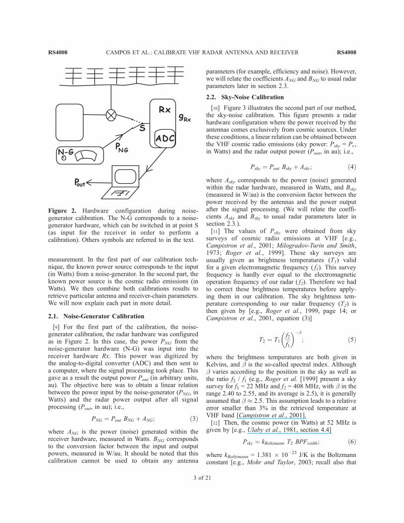
measurement. In the first part of our calibration tech-nique, the known power source corresponds to the input(in Watts) from a noise-generator. In the second part, theknown power source is the cosmic radio emissions (inWatts). We then combine both calibrations results toretrieve particular antenna and receiver-chain parameters.We will now explain each part in more detail.

2.1. Noise-Generator Calibration

[9] For the first part of the calibration, the noise-generator calibration, the radar hardware was configuredas in Figure 2. In this case, the power PNG from thenoise-generator hardware (N-G) was input into thereceiver hardware Rx. This power was digitized bythe analog-to-digital converter (ADC) and then sent toa computer, where the signal processing took place. Thisgave as a result the output power Pout (in arbitrary units,au). The objective here was to obtain a linear relationbetween the power input by the noise-generator (PNG, inWatts) and the radar power output after all signalprocessing (Pout, in au); i.e.,

PNG ¼ Pout BNG þ ANG; ð3Þ

where ANG is the power (noise) generated within thereceiver hardware, measured in Watts. BNG correspondsto the conversion factor between the input and outputpowers, measured in W/au. It should be noted that thiscalibration cannot be used to obtain any antenna

parameters (for example, efficiency and noise). However,we will relate the coefficients ANG and BNG to usual radarparameters later in section 2.3.

2.2. Sky-Noise Calibration

[10] Figure 3 illustrates the second part of our method,the sky-noise calibration. This figure presents a radarhardware configuration where the power received by theantennas comes exclusively from cosmic sources. Underthese conditions, a linear relation can be obtained betweenthe VHF cosmic radio emissions (sky power: Psky = Pr,in Watts) and the radar output power (Pout, in au); i.e.,

Psky ¼ Pout Bsky þ Asky; ð4Þ

where Asky corresponds to the power (noise) generatedwithin the radar hardware, measured in Watts, and Bsky

(measured in W/au) is the conversion factor between thepower received by the antennas and the power outputafter the signal processing. (We will relate the coeffi-cients Asky and Bsky to usual radar parameters later insection 2.3.).[11] The values of Psky were obtained from sky

surveys of cosmic radio emissions at VHF [e.g.,Campistron et al., 2001; Milogradov-Turin and Smith,1973; Roger et al., 1999]. These sky surveys areusually given as brightness temperatures (T1) validfor a given electromagnetic frequency ( f1). This surveyfrequency is hardly ever equal to the electromagneticoperation frequency of our radar ( f2). Therefore we hadto correct these brightness temperatures before apply-ing them in our calibration. The sky brightness tem-perature corresponding to our radar frequency (T2) isthen given by [e.g., Roger et al., 1999, page 14; orCampistron et al., 2001, equation (3)]

T2 ¼ T1f2

f1

� ��b

; ð5Þ

where the brightness temperatures are both given inKelvins, and b is the so-called spectral index. Althoughb varies according to the position in the sky as well asthe ratio f2 / f1 (e.g., Roger et al. [1999] present a skysurvey for f1 = 22 MHz and f2 = 408 MHz, with b in therange 2.40 to 2.55, and its average is 2.5), it is generallyassumed that b � 2.5. This assumption leads to a relativeerror smaller than 3% in the retrieved temperature atVHF band [Campistron et al., 2001].[12] Then, the cosmic power (in Watts) at 52 MHz is

given by [e.g., Ulaby et al., 1981, section 4.4]

Psky ¼ kBoltzmann T2 BPFwidth; ð6Þ

where kBoltzmann = 1.381 � 10�23 J/K is the Boltzmannconstant [e.g., Mohr and Taylor, 2003; recall also that

Figure 2. Hardware configuration during noise-generator calibration. The N-G corresponds to a noise-generator hardware, which can be switched in at point S(as input for the receiver in order to perform acalibration). Others symbols are referred to in the text.

RS4008 CAMPOS ET AL.: CALIBRATE VHF RADAR ANTENNA AND RECEIVER

3 of 21

RS4008

J/K = W/(Hz K)], and BPFwidth is the band-pass filterwidth of the radar receiver, in Hertz. The derivation ofequation (6) takes into account the facts that the cosmicradiation is unpolarized, and that our linearly polarizedantenna will then collect half of the incident (unpolar-ized) cosmic power [Ulaby et al., 1981].[13] This sky-noise calibration only provided informa-

tion about the antenna and receiver parameters in ageneral sense. Particular values such as antenna efficiencyor receiver-chain noise could not be retrieved in thismanner. However, we were able to retrieve these antennaand receiver-chain parameters by combining both thesky-noise calibration and noise-generator calibrationmethods. The next section explains the procedure.

2.3. Combining Both Calibration Methods

[14] Particular expressions for antenna and receiver-chain parameters were derived by combining equations

(1), (2), (3), and (4). Starting from equations (2) and (3),with PRx = PNG:

�NRx

gRxþ Pout

gRx¼ ANG þ BNG Pout )

gRx ¼1

BNG

ð7Þ

and

NRx ¼ �ANG gRx ¼�ANG

BNG

: ð8Þ

As well, from equations (1) and (2):

Pr eR gRx þ Na gRx þ NRx ¼ Pout )

Pr ¼� Na gRx þ NRxð Þ

eR gRxþ 1

eR gRxPout:

ð9Þ

From equations (4) and (9), with Pr = Psky:

Bsky ¼1

eR gRx:

Then, from equation (7):

eR ¼ BNG

Bsky

: ð10Þ

Also, from equations (4) and (9):

Asky ¼� Na gRx þ NRxð Þ

eR gRx) Na ¼ �Asky eR þ

NRx

gRx:

Then from equations (7), (8), and (10):

Na ¼ �Asky

BNG

Bsky

� ANG: ð11Þ

[15] In addition, expressions for the uncertainties in theantenna and receiver estimates (eR, Na, gRx, and NRx)were derived from the following expression [e.g., Presset al., 1986, page 505]:

s 2 fð Þ ¼XNi¼1

s 2 xið Þ @f

@xi

� �2

; ð12Þ

where s2( f ) is the variance uncertainty of the function f,which is a function that depends on variables x1, x2,. . .,xn�1, xn. As well, s2(xi) is the variance uncertainty forthe i-th variable. Equation (12) was then applied toequations (7), (8), (10), and (11) in order to obtain thefollowing one-standard-deviation uncertainties:

s gRxð Þ ¼ s BNGð ÞB2NG

; ð13Þ

Figure 3. Hardware configuration during sky-noisecalibration.

ð7Þ

RS4008 CAMPOS ET AL.: CALIBRATE VHF RADAR ANTENNA AND RECEIVER

4 of 21

RS4008

s NRxð Þ ¼

ffiffiffiffiffiffiffiffiffiffiffiffiffiffiffiffiffiffiffiffiffiffiffiffiffiffiffiffiffiffiffiffiffiffiffiffiffiffiffiffiffiffiffiffiffiffiffis2 ANGð ÞB2NG

þ s2 BNGð ÞA2NG

BNG4

s; ð14Þ

s eRð Þ ¼ffiffiffiffiffiffiffiffiffiffiffiffiffiffiffiffiffiffiffiffiffiffiffiffiffiffiffiffiffiffiffiffiffiffiffiffiffiffiffiffiffiffiffiffiffiffiffiffis2 BNGð ÞB2sky

þ s2 Bsky

� �B2NG

Bsky4

s; ð15Þ

s Nað Þ

¼ffiffiffiffiffiffiffiffiffiffiffiffiffiffiffiffiffiffiffiffiffiffiffiffiffiffiffiffiffiffiffiffiffiffiffiffiffiffiffiffiffiffiffiffiffiffiffiffiffiffiffiffiffiffiffiffiffiffiffiffiffiffiffiffiffiffiffiffiffiffiffiffiffiffiffiffiffiffiffiffiffiffiffiffiffiffiffiffiffiffiffiffiffiffiffiffiffiffiffiffiffiffiffiffiffiffiffis2 Asky

� � B2NG

B2sky

þs2 BNGð Þ A2sky

B2sky

þ s2 Bsky

� � A2skyB2NG

B4sky

þ s2 ANGð Þr

;

ð16Þ

where the values for s2(Asky), s2(Bsky), s2(ANG), ands2(BNG) were obtained from the square of uncertaintiesin the coefficients of equations (3) and (4). Notice thatthe uncertainties in Pout are already considered when wecompute the uncertainties in coefficients ANG, BNG, Asky,and Bsky.[16] Therefore the antenna and receiver-chain para-

meters were found from equations (7), (8), (10), and(11); and the corresponding uncertainties were computedfrom equations (13), (14), (15), and (16).

2.4. Computing Calibrated Power Spectra

[17] Once we have the calibration of the radar mea-sured power (Pout), we proceed with a calibration of thepower densities. To do this we produce Doppler spectrafrom a recorded time series and then proceed as follows.We assume that the spectra are recorded at steps Df.Then, from equation (4) we know that

Df ½Ssky f1ð Þ þ Ssky f2ð Þ þ . . .þ Ssky fnð Þ¼ Asky þ BskyDf Sout f1ð Þ þ Sout f2ð Þ þ . . .þ Sout fnð Þ½ ;

where Df is the spectral bin resolution (in Hz). Thevariables Sout(fi) and Ssky(fi) correspond to the Dopplerpower densities at the i-th spectral bin (a total of nspectral bins), given in au/Hz for the variables with thesubscript ‘‘out’’ and in W/Hz for the variables with thesubscript ‘‘sky’’. The previous equation can also beexpressed asXn

i¼1

Ssky fið Þ ¼Xni¼1

1

n

Asky

Dfþ Bsky Sout fið Þ

:

Therefore the power-densities calibration equation forthe i-th spectral bin is given by

Ssky fið Þ ¼ 1

n

Asky

Dfþ Bsky Sout fið Þ : ð17Þ

Note that, for the derivation of equation (17), the linearrelation in equation (4) must be applied for the powers inlinear units.

[18] It is not rare to have radar signal processingperforming coherent averaging (for example, in theMcGill VHF radar). Under these conditions, the fullspectral range is defined by the radar sampling rate asfollows:

fsampling ¼PRF

Ncoh

; ð18Þ

where PRF is the radar pulse repetition frequency andNcoh is the number of samples used for the coherentaverages (given in Table 1).[19] Another common signal processing practice (also

performed by the McGill VHF radar) is to store onlyDoppler power spectra within a range of interestingfrequencies [i.e., Sout’ (fi)]. If the full spectral range[i.e., Sout(fi)] corresponds to Doppler frequencies within± 0.5 fsampling, then the quantity Pout, corresponding tothe full spectral range, is given by

Pout ¼ P 0out

fsampling

DSR¼ P 0

out � PRF

DSR� Ncoh

; ð19Þ

where

Pout ¼Xþfsampling=2

f¼�f sampling=2

Sout fð Þ ;

P 0out ¼

XþDSR=2

f¼�DSR=2

S0out fð Þ ;

and Pout0 is the total power integrated within the stored

Doppler spectral range (DSR).[20] Equation (17) has then to be modified according

to equations (18) and (19). For this, we use the fact thatthe power density is conserved for a white-noise spec-trum. As well, we recognize that the application ofcoherent averaging (of in-phase and quadrature timeseries, as it is done in our signal processing) reducesboth the full spectral range [reduction already included inthe definition of fsampling; i.e., equation (18)] and themeasured Psky (since the spectral density magnitude ispreserved at all frequency bins; e.g., Lyons [1997,p. 321]). Therefore the calibrated power-density spectra,Scal, at the frequency bin fi, must be such that

1

Ncoh

Psky

fsampling¼

Pni¼1

D f Scal fið Þ½

DSR; ð20Þ

where Ncoh is the number of samples used for thecoherent averages, Df is the spectral bin resolution, andPsky is given in Watts. From here, n is the number ofstored spectral bins (not longer the total number of bins).

RS4008 CAMPOS ET AL.: CALIBRATE VHF RADAR ANTENNA AND RECEIVER

5 of 21

RS4008

In addition, equation (4) provides us with a conversionbetween Watts and arbitrary units. Therefore fromequations (4) and (20) we obtain that

Asky þ BskyPout

Ncoh fsampling¼ Df

DSR

Xni¼1

Scal fið Þ : ð21Þ

However, from Equation (19) we know that

Pout

fsampling¼

Xni¼1

Df S0out fið Þ� DSR

; ð22Þ

where Sout’ ( fi ) is the measured spectral density (in au/Hz)at the Doppler frequency bin fi. Then, by combiningequations (21) and (22), we have that

Asky

Ncohfsamplingþ Bsky

Ncoh

Xni¼1

Df S0out fið Þ� DSR

¼ Df

DSR

Xni¼1

Scal fið Þ; ð23Þ

) DSR Asky

DfNcohfsamplingþ Bsky

Ncoh

Xni¼1

S0out fið Þ¼Xni¼1

Scal fið Þ;

)Xni¼1

1

n

DSR Asky

Df Ncoh fsampling

þXni¼1

Bsky

Ncoh

S0out fið Þ

¼Xni¼1

Scal fið Þ:

Since Df = DSR / n, we thus get,

Scal fið Þ ¼ Asky

fsamplingþ Bsky S

0out fið Þ

1

Ncoh

: ð24Þ

2.5. Operational Background

[21] To show the application of our method we useddata from the McGill VHF radar [described by Camposand Hocking, 2003] working under the configuration

described in Table 1. For the sky-noise calibration, wecould use any oblique direction as well, but the verticaldirection already provides enough observations to suc-cessfully calibrate the radar. Our radar system carefullymonitors, on a regular basis, the offset and quadrature ofthe real and imaginary channels. The nonorthogonality ofthese channels introduces small errors on instantaneouspower estimates, which are always less than about 10%.As well, the analog-to-digital converter uses a 16-bitdigitizer, and typical recorded amplitudes are at least twoorders of magnitude greater than the digitalization reso-lution. Therefore the errors (on instantaneous powerestimates) at the ADC level (induced by the data quan-tization) are in the order of 1% or less. Notice that allthese errors do not introduce biases in our VHF precip-itation measurements.[22] The signal processing used here was the same as

in the work of Hocking [1997, section 4]. Every 35 s, aprofile of 45 Doppler power spectra (300-point discrete-spectrum within a spectral range of ± 10.0 Hz, for45 range gates between 0.5 and 23.0 km) was pro-duced. We integrated each of these spectra in order toobtain corresponding Pout’ values; i.e., the integratedpowers (in au) within the Doppler spectral range(DSR, see Table 1).[23] As described in section 2.1, during the noise-

generator calibration, a small modification was made inthe reception hardware. The noise-generator output wasconnected to the receiver, instead of the line from thetransmitter-receiver switch. Then, different noise sourceswere obtained by changing the factor F in the noise-generator hardware. One unit increment in F was equiv-alent to a 290-Kelvin increase in brightness temperature.At F = 0, the noise generator still introduces a smallamount of power into the receiver. This amount dependson the noise generator temperature (approximately290 K) in a manner similar to equation (6). Thereforepower input by the noise generator into the radar receiverwas given by:

PNG ¼ F þ 1ð Þ 290Kð ÞkBoltzmann BPFwidth; ð25Þ

where PNG is the noise-generator power (in Watts,measured in the radar receiver just after the band-passfilter). As before, kBoltzmann is the Boltzmann constantand BPFwidth is the band-pass filter width of the radarreceiver (given in Table 1), in Hertz.[24] For the second part of our calibration, there was

no need to disconnect the transmitter, or to alter thenormal operation of the radar in any way. We kept theradar hardware and software working as usual (i.e., withline from transmitter-receiver switch connected toreceiver, as in Figure 1). The known power sources fromcosmic radio emissions (in Watts) were then comparedwith the corresponding radar integrated power (in au)

Table 1. McGill VHF Radar Parameters

Parameter Value

Beam Direction VerticalTransmitted Wavelength (Frequency) 5.77 m (52.0 MHz)Peak Transmitted Power 40 kWOne-Way Half-Power Half-Beam Width 2.3�Pulse Duration 3.5 msPulse Repetition Frequency (PRF) 6.0 kHzBand Pass Rx Filter Width (BPFwidth) 400 kHzNumber of Coherent Averages (Ncoh) 16Doppler Spectral Range

(DSR, After Signal Processing)20 Hz

Time Resolution Approx. 35 s/profileSpectral Bin Resolution (Df ) 0.0667 HzLocation (Lat., Long.) 45.409� N, 73.937� W

RS4008 CAMPOS ET AL.: CALIBRATE VHF RADAR ANTENNA AND RECEIVER

6 of 21

RS4008

measured only at very high range gates (between 17.5and 22.5 km). At these ranges, backscattering of thetransmitted power and other terrestrial VHF radio sour-ces is negligible. Thus the radar received powers, at thesehigh ranges only, were considered as coming exclusivelyfrom cosmic sources.

3. Results

3.1. Noise-Generator Calibration

[25] The noise-generator calibration was performedusing observations made on 21 October 2004, a daywithout precipitation. The results are presented inFigure 4. For a given PNG value, there are 45 Pout’values plotted in the x axis. These Pout’ values corre-spond to the 45 radar range gates (between 0.5 and23.0 km) available at each profile. Considering the300 spectral points and the 45-range gates used forcomputing Pout’ , we estimate [from Petitdidier et al.,1997, equation (10)] that the expected error in these

computations is 100%

� ffiffiffiffiffiffiffiffiffiffiffiffiffiffiffiffiffiffi300� 45

p 1 %. We then

computed the Pout values plotted in the abscissa (x axis)of Figure 4 by using equation (19). The range of Fvalues, from 0 to 30 units, was sampled twice (the twodata sets are represented in Figure 4 as small crosses). AChi-square linear fit [Press et al., 1986, section 14.2]was then used to obtain the relation

PNG ¼ �3:420� 10�15 � 6:7� 10�17� �

W½ þ Pout 9:250� 10�21 � 2:3� 10�23

� �½W=au;

ð26Þ

where the units are given in square brackets, and theuncertainties correspond to one standard-deviation errorsin the coefficients estimates. The relationship (26) ispresented as a line in Figure 4.

3.2. Cosmic-Noise Calibration

3.2.1. Sky Map[26] The cosmic noise power Psky at the radar operating

frequency (52 MHz) was obtained from a sky brightnesstemperatures map at 45 MHz (the closest availablefrequency). We used data published by Campistron etal. [2001], which corresponds to epoch-J1999 equatorial-coordinates. These coordinates, right ascension and dec-lination, are continuously changing in time, primarily asa result of the precession of the equinoxes. We then hadto convert the figure coordinates from the epoch J1999 tothe epoch J2004 (the epoch of the radar observations).For this, we used the standard procedure given in sectionB42 of The Astronomical Almanac [Nautical AlmanacOffices et al., 2003]. The resulting sky map is presented

in Figure 5, which has a resolution of 1.5 min in right-ascension hour and one degree in declination angle.[27] To test the reliability of this 45 MHz map, we

compared its brightness temperatures at a particulardeclination angle (matching our VHF radar observa-tions) with the corresponding values from the maps byMilogradov-Turin and Smith [1973] and by Roger et al.[1999]. The first map corresponds to a 38-MHz frequen-cy and epoch J1967, and the second map corresponds to22-MHz frequency and epoch B1950. For this compar-ison, we then had to convert the 45, 38, and 22 MHztemperatures to 52 MHz by using equation (5) with b =2.5. As well, we had to precess the coordinates to acommon astronomical epoch, in this case J2004 (theepoch of our VHF radar observations). Finally, we uselinear interpolation in order to obtain the temperaturevalue at the declination of 45.409� and with a rightascension resolution of 0.25 hours. Figure 6 presents the

Figure 4. Result of the noise-generator calibration. Theleft-side y axis is the noise-generator factor F, which isrelated to the right-side y axis, the power PNG, byequation (25). For every PNG value, there are 45 Pout

values (corresponding to 45 radar range gates), which arecomputed from equation (19) and plotted in the x axis.The linear relation in equation (26) is given by the line,and it is obtained from two calibration experiments(990 observations in total).

RS4008 CAMPOS ET AL.: CALIBRATE VHF RADAR ANTENNA AND RECEIVER

7 of 21

RS4008

comparison of sky brightness temperatures for the threemaps. The only significant disagreement is with the22 MHz map, at right ascension between 19 and22 hours, probably due to contamination by the strongsignal from Cygnus A. However, there is general agree-ment between the three sky maps, which indicates thereliability of the 45-MHz map.[28] Considering our radar antenna pattern and time

resolution, the radar observations and the sky map didnot match in resolution (the data sets representativenessare not the same). Therefore the sky brightness temper-atures, at the radar declination, were smoothed in orderto resemble our VHF radar resolution. We did this byconvolving the 45-MHz map (Figure 5) with a directnumerical simulation of the one-way antenna pattern(i.e., the antenna one-way polar-diagram). This antennapattern was provided by the radar manufacturer (MardocInc., of London, Ontario, Canada) and it is presented inFigure 7. Notice that, as the kernel of the convolutionoperation, we used only a section of the full antennapattern (zenith angles smaller than 13�, having the sameresolution as the sky map, i.e., 1.5 min per 1�). Zenithangles greater than 13� were not used since they imply akernel outside the sky map. In any case, the sidelobes ofthe antenna pattern located outside 12� zenith angles arenot significant (their magnitudes are generally smallerthan �15 dB). For all right ascension hours (at aresolution of 1.5 min), the convolution was performed

with the kernel centered at the declination of our radarobservations (i.e., 45.409� declination angle, at thedashed line in Figure 5). The result for this convolution,between the sky brightness temperatures and the antennapattern, was used as input for equation (5). The resulting52-MHz brightness-temperatures are plotted in Figure 9as the red line.3.2.2. Sky Noise[29] Between 14 and 17 October 2004, the McGill

VHF radar was operated according to the specificationsgiven in Table 1. We selected the period in Figure 8,where the sky noise could be assumed to be due only tocosmic sources. From the measured Doppler powerspectra, we computed the total integrated power (forspectral Doppler frequencies between �10.0 Hz and+10.0 Hz) at ranges between 17.5 and 22.5 km. At thesehigh ranges, the Doppler power spectra received by VHFradars are basically formed by white noise, and when weintegrate these spectra we obtain the so-called sky noise.We then used equation (19) to correct the total integratedpower for not storing the full Doppler spectra. Consid-ering the 300 spectral points and the 11 range gates usedfor computing the total power of the sky noise, weestimate [from Petitdidier et al., 1997, equation (10)]that the expected error in these computations is

100%

� ffiffiffiffiffiffiffiffiffiffiffiffiffiffiffiffiffiffi300� 11

p 2 %. Notice in Figure 8 that the

Figure 5. Epoch-corrected sky survey at 45 MHz.

RS4008 CAMPOS ET AL.: CALIBRATE VHF RADAR ANTENNA AND RECEIVER

8 of 21

RS4008

temporal evolution of the sky noise power has a 23-hours-56-min cycle (i.e., a sidereal day). This confirmsthe dominant cosmic origin of the noise observed by ourVHF radar.[30] In some cases, a few extreme, spurious power

observations can be measured by VHF radars, and theseobservations correspond to signals from noncosmicsources (for example, human interference or broadcast-ing). These signals must be eliminated before proceedingwith our calibration. In Figure 8, we have already filteredout most of these spurious data by eliminating sky noisevalues that were six or more median-absolute-deviationsaway from the median sky noise (the median for thewhole observation period).[31] By knowing the direction in the sky at which our

radar is pointing at a given time, we can compute theequatorial coordinates (right ascension and declination)of this direction. We computed the radar pointing direc-tions (for the cosmic sky-noise periods in Figure 8) byusing standard astronomical procedures valid for theepoch J2004 [e.g., Lang, 1999]. Since our radar was

located at a fixed longitude and elevation angle (verticaldirection), our cosmic sky noises correspond to a fixeddeclination with varying right ascension. This is shownin Figure 9, where the VHF cosmic sky-noises (blackand blue points, in 105 au) are plotted as a function ofright ascension. Since our radar measurements corre-spond to a declination of 45.409�, we can compare ourintegrated powers with the corresponding 52 MHz skybrightness temperatures computed in section 3.2.1. Thesetemperatures are over-plotted in Figure 9 as red points (inkiloKelvins).[32] The black observations in Figure 9, which corre-

spond to nighttime radar-measurements taken between23.1 UTC (7:06 pm local time) and 11.1 UTC (7:06 amlocal time), match well with the corresponding skytemperatures (red points). However, the observations inblue, which corresponds to daytime measurements takenbetween 11.1 UTC and 23.1 UTC, tend to be above thecorresponding sky brightness temperatures. For radiowaves, daytime sky-noise is very challenging to analyze.On one hand, we have the power contribution from theSun, which for our VHF band corresponds to a bright-ness temperature in the order of 105 K [Subramanian,2004]. This temperature corresponds to about 10�13

Watts [from equations (5) and (6)]. On the other hand,there is the ionospheric absorption of radio waves, whichaffects all cosmic radiation when passing through the Dand E ionospheric layers (at 60- to 100-km altitude).Ionospheric absorption is a well-known phenomenon,which is controlled in part by solar activity (i.e., sunspotnumber). Observations taken during the night are prac-tically free from these inconveniences. We thereforefiltered out all the measurements taken between7:06 am and 7:06 pm (i.e., approximately betweensunrise and sunset).3.2.3. From Arbitrary Units to Watts[33] In order to obtain the sky-noise powers, the

brightness temperatures (red points) in Figure 9 weremultiplied by the Boltzman constant and the radar Band-Pass-Filter width [i.e., equation (6)]. However, the radarmeasurements (black points) in Figure 9 still had a largeamount of scatter, which could complicate the empiricalderivation of the coefficients in equation (4). We reducedthis scatter in the following manner: for each Psky

observation (in Watts), we selected all radar observations(black points in Figure 9, in arbitrary units) that werewithin 45 s around the Psky hour angle. (Recall that theresolution of the Psky observations is 1.5 min.) Themedian of these radar observations was then the radaroutput power, Pout, to be matched to the Psky observation.The matched pairs are shown in Figure 10 as rightascension time series, where the line corresponds to thesky-noise powers (Psky, in Watts), and the points corre-spond to the Pout values (in arbitrary units).

Figure 6. Comparison of 52 MHz sky brightnesstemperatures at 45.409� declination. It is obtained byapplying equation (5), with b = 2.5, to the data in skysurveys at 45 MHz (in dotted line), 38 MHz (in dashedline), and 22 MHz (in continuous line).

RS4008 CAMPOS ET AL.: CALIBRATE VHF RADAR ANTENNA AND RECEIVER

9 of 21

RS4008

[34] To eliminate the unlikely possibility of having alag between the two time series in Figure 10, wecomputed the cross correlation between the two series.The maximum cross correlation was found at lag timeequal zero (not shown). This means that no time lag canbe found between the two time series, and if there is one,it will be less than the interval between two consecutiveobservations (i.e., 1.5 min). Thus no lag-time correctionwas applied.[35] Figures 9 and 10 indicate minor departures

between observed and expected sky noise patterns (Pout

and Psky, respectively). We have minimized these depar-tures by filtering out spurious observations, using themethods described in section 3.2.2. Small remainingdepartures, however, can be due to small, spurious powerobservations from noncosmic sources, to small depar-tures of the cosmic sources from the corresponding sky-map values, to local departures in the spectral index (b)from its average 2.5 value, and to changes in the iono-spheric composition [e.g., Campistron el al., 2001].[36] We can also visualize the data in Figure 10 by

plotting Psky as a function of Pout. This leads to thescatterplot in Figure 11 and the linear relation for powerin Watts as a function of power in arbitrary units (the linein the figure). As described in section 2.2, we expect alinear relation, but the uncertainties about the variation ofb in space [see equation (5)] could deviate the expectedlinear relation slightly. Fortunately, Figure 11 indicatesthat this small effect can be neglected in our case.

Therefore a linear relation between power in Watts andpower in arbitrary units was derived by minimizing theChi-square error statistic, as in Press et al. [1986], and itis given as follows:

Psky ¼ �1:797� 10�14 � 9:4� 10�16� �

W½ þ Pout 2:095� 10�20 � 3:6� 10�22

� �½W=au:ð27Þ

As before, the units are given in square brackets, and theuncertainties correspond to one standard-deviation errorsin the coefficients estimates.

3.3. Radar Hardware Coefficients

[37] In order to calculate the values of antenna andreceiver-chain parameters, we need to compare our twosets of calibration equations [i.e., the sky-noise calibra-tion in equation (27) and the noise-generator calibrationin equation (26)]. The comparison is shown in Figure 12,where the sky-noise calibration is plotted as a dashedline and the noise-generator calibration is given as acontinuous line. Of course, the slope of the noise-generator calibration is smaller than the slope of thesky-noise calibration, and we expect this difference fromequation (10).[38] The hardware parameters can now be computed

from equations (7), (8), (10), and (11) simply by noticingthe correspondence between equations (4) and (27), andbetween (3) and (26). As well, their corresponding

Figure 7. Kernel of convolution between the sky map and the radar antenna pattern.

RS4008 CAMPOS ET AL.: CALIBRATE VHF RADAR ANTENNA AND RECEIVER

10 of 21

RS4008

uncertainties are estimated from equations (13) to (16).These values are given in Table 2. Notice that theantenna efficiency in Table 2, eRx = 44%, refers onlyto reception. The antenna system was originallydesigned to maximize transmitted power, and the overallpower losses on transmission are estimated to be lessthan 2 dB; i.e., eT = 63%.[39] To compute the noise temperature of the receiver

chain, TRx, we use an equation similar to equation (6);i.e., NRx(W) = kBoltzmannTRx BPFwidth, where NRx(W) isthe receiver-chain noise expressed in units of Watts. Thisreceiver-chain noise can be computed from the NRx valuein Table 2 and the slope in equation (26), or from the

offset in equation (26). In both cases, we obtain that thenoise temperature of the receiver chain (for the McGillradar) is about 619 ± 12 K.

4. Antenna Matching Unit

[40] To validate our results, we will now study thevarious subcomponents of the radar antenna that aremost likely leading to power losses. This analysis leadsto a third calibration method, which will provide anindependent estimation of the antenna efficiency.[41] In this regard the antenna transmission lines are

the most important. In order to minimize energy losses,the impedance in the antenna aerials is matched to the

Figure 8. Example of a time series (in UTC) for sky-noise power [spectral integral within theDoppler spectral range and corrected by equation (19)] measured by the McGill VHF radar, withthe beam at vertical direction, at ranges between 17.5 and 22.5 km, from 14 (starting at 22:50 UTC)to 17 (ending at 13:30 UTC) October, 2004.

RS4008 CAMPOS ET AL.: CALIBRATE VHF RADAR ANTENNA AND RECEIVER

11 of 21

RS4008

transmitter impedance through an arrangement of coaxialcables. These assemblies of cables are then called theantenna matching units. For the McGill VHF radar, weuse a matching arrangement like the one shown inFigure 13. This includes matching cables made fromRG213 coaxial cable, with lengths as indicated in thefigure, and beam-pointing boxes that are used to intro-duce phase delays to the antennas in order to implementbeam pointing. The internal details of the beam-pointingboxes are not shown on the figure, but the efficiency ofthese units will be considered separately in due course.The matching boxes at the transmitter end hold inductorsof approximately 75 nH and capacitors to earth of about60 pF, which are tunable in order to provide finalaccurate matching.

[42] The arrangement in Figure 13 includes matchingboxes and switching boxes. In order to assess theperformance of this arrangement, we have built a slightlysimpler system which contains no switching boxes, andused it for performing the third calibration method. Thisarrangement is shown in Figure 14. We will first discussthe operation of this unit, and consider theoreticalefficiencies. Following this, we will report the resultsof a series of measurements on the system, and comparewith theory. Finally, we will return to the originalmatching arrangement (Figure 13) and make furthermeasurements, which can then be interpreted in termsof our results using Figure 14.[43] In order to properly understand the efficiency of

an impedance matching system, like that shown in

Figure 9. Cosmic sky noise measured by the McGill VHF radar. These correspond to nearly 63hours of observations during conditions of negligible noncosmic VHF radio sources (between 14and 17 October, 2004). The left-side y axis and the points correspond to radar measurements atranges between 17.5 and 22.5 km. (The black points were measured during nighttime, between23.1 UTC and 11.1 UTC. The blue points correspond to observations taken during the remainingdaytime periods, between 11.1 and 23.1 UTC.) The red line and rightside y axis are obtained fromthe temperature values at the dashed line in Figure 5 (i.e., a declination of 45.409�), the radarantenna pattern in Figure 7 (i.e., the convolution kernel), and equation (5) with b = 2.5.

RS4008 CAMPOS ET AL.: CALIBRATE VHF RADAR ANTENNA AND RECEIVER

12 of 21

RS4008

Figure 14, it is necessary to consider both its forward andbackward transmission characteristics. The cable imped-ance is assumed to be 50 W. The simplified transmissionlines shown in Figure 14 had cables lengths of one halfof a wavelength between H and I, one quarter of awavelength between G and F, one half of a wavelengthbetween E and D, and one quarter of a wavelengthbetween C and B. We assume that the antennas are alltuned to 50 W. Where two cables come together as atG/H, the point G (looking out toward the antenna aerials)sees an impedance of 25 W. The quarter wave sectionF-G transforms this to 100 W. The point E, looking outtoward the antenna aerials, sees an effective impedanceof 2 � 100 W impedances in parallel, or 50 W. The pointD, looking out toward the antenna aerials, also sees 50 W.Point C sees 2 � 50 W impedances in series, and so sees25 W. This maps to 100 W at B (looking toward theantenna aerials). Finally, point A sees 2 � 100 Wimpedances in parallel, or 50 W. These results aresummarized in the fourth column of Table 3.[44] The fifth column in Table 3 shows actual measure-

ments of the impedances, expressed as magnitudesand angles, as measured by a Hewlett-Packard Vector-

Impedance Meter. Agreement with theoretical expect-ations is good, and differences are due to the facts that(1) the characteristic impedance of the cable was actuallyclose to 51 W and (2) slight errors in cutting the lengthsof the cables to exact multiples of a quarter of awavelength. (Optimal cable lengths were determinedusing a vector-impedance meter, with the cables beingopen circuit. The quarter-wavelength cables were cutuntil impedance was zero, and the half-wavelengthcables were cut until impedance was maximum.)[45] In the previous paragraph we examined imped-

ance transformations in the matching unit, comparingtheoretical and experimental values. It is also necessaryto examine power transmission, which is best done bylooking at voltages at various points along the antennatransmission lines.[46] A continuous-wave 52.00-MHz signal, of peak-to-

peak voltage equal to 1.16 V (as measured into aCathode Ray Oscilloscope loaded with 50 W), was fedinto the point A in Figure 14. In addition, all terminationsexcept that at ‘‘I’’ were given 50 W loads. The voltagemeasured into a 50 W load at ‘‘I’’ was then equal to28-mV peak to peak. It would be expected that theapplied power should be equally distributed across allloads, so that if the input power is 1

2� 1:162

50, then the

output voltage should be 29 mV. The total cable lengthfrom input to output is 1.5 wavelengths, or 5.71 m, sincethe velocity propagation factor for RG213 cable is 0.66.This RG213 coaxial cable has a loss factor of 1.3 dB per30 m at 52 MHz, so losses of 0.25 dB are expected. Thisshould reduce the received signal to a peak voltage of28.2 mV, consistent with our measured value. Hence thelosses on transmission through such a matching unit areabout 0.2 dB, mainly due to cable attenuation.[47] In considering the system efficiency of a transmit-

receive system like this, it is also necessary to considerthe return path of the signal. It is well known that with awell-designed antenna array, the sky noise received bythe radar is independent of the number of antenna aerials,provided that the sky noise is isotropic in origin. Supposethat a single antenna aerial is used, and fed directly intopoint A in Figure 14, from where it passes through atransmit-receive switch to a receiver. Let the signalpower received be P. Now suppose that 16 antennaaerials are now used, and are fed by the matchingarrangement in Figure 14. Each antenna aerial receivespower P, but as the signal passes back through the stagesof the matching unit, more and more is lost by reflec-tions. Some of it ends up being reradiated by otherantenna aerials in the array. In fact, the power expectedat the point A due to the signal received at one antenna isonly P/16. The accumulated power from all antennaaerials is 16 times this, or P. In terms of polar diagrams,this result can be determined by recognizing that thecollection of 16 antenna aerials has a narrower polar

Figure 10. Expected and measured cosmic powers.The points and the left-side Y-axis (Pout, in 105 au) areobtained from median values of the radar measurements(black points in Figure 9). The line and the right-side yaxis (Psky, in 10�14 Watts) are obtained from equation (6)and the brightness temperatures in Figure 9.

RS4008 CAMPOS ET AL.: CALIBRATE VHF RADAR ANTENNA AND RECEIVER

13 of 21

RS4008

diagram than a single antenna aerial, but in terms of theactual matching used, the result arises because of powerlosses due to reflections on the return path. The receivedsignal strength (and therefore the sky-noise temperature)is thus independent of the number of antenna aerialsused. This is a well-known result that is employed incalibrating many radio systems, and it has been used inthe early sections of this paper as well.[48] To see this more clearly, it is a simple matter to

determine the impedances seen at various stages of thematching path looking back toward the transmitter (asopposed to the previous cases, which were determinedlooking out toward the antenna aerials). To begin,consider the point B (in Figure 14) looking back towardthe transmitter. It sees a 50-W load in the form of thetransmitter, and a 100-W load coming in from the otherarm of the V-section closest to the transmitter. Hencepoint B sees 33.3 W. This maps to 75 W at point C due to

the quarter-wavelength section. By working along thematching unit from A to I, the impedances seen in thesecond column of Table 3 can easily be deduced. InTable 3, column 3 shows experimental values of theimpedances, and again agreement between theory andexperiment is good.[49] It is now necessary to determine the power

expected to be received at the point A, assuming thatthis point is terminated in 50 W, and all other cablesabove the point I in Figure 14 are also terminated in50 W. This can be calculated by looking at transmissionefficiencies at each point. For example, a 50-W inputapplied at point I sees an impedance of 27.25 W, so avoltage reflection coefficient of (50 � 27.25)/(50 +27.25) = 0.2945 applies. Hence the reflected power is8.7% of the original. The transmitted power is therefore91.3% of the original. This transmitted signal progressesto the junction between G and H, where some signal

Figure 11. Scatterplot of expected versus measured cosmic sky-noise power. The y axis values(Psky, in 10-14 Watts) correspond to the line in Figure 10. The x axis values (Pout, in 105 au) are thecorresponding points in Figure 10. The line here corresponds to equation (27).

RS4008 CAMPOS ET AL.: CALIBRATE VHF RADAR ANTENNA AND RECEIVER

14 of 21

RS4008

passes through to G, some is reflected back, and yet moreof the signal passes into the adjoining cable and istransmitted into the next termination (or, in a real radar,is transmitted into the next antenna aerial). The signalthat is reflected back to I is partly retransmitted from Iinto the adjoining load, and partly rereflected back to H,and so forth. The signal that passes through G suffersfurther reflection and splitting at E/F, and so forth.Eventually, only one sixteenth of the original signalarrives at the point A.[50] Experimental testing of this pathway was carried

out. An input signal of 1.16 V peak-to-peak fed in at ‘‘I’’produced a signal of 0.26V peak-to-peak at point A.Inserting inputs at other locations similar in location topoint ‘‘I’’ gave outputs at the point A in the range 0.24 to0.27 V peak-to-peak. These results are entirely consistentwith the above expectations, and indicate that even onthe return path the losses of this matching unit are verymodest, and certainly less than 10%, even includinglosses due to cable attenuation.

[51] We now return to Figure 13. Having performedthe above tests, a subunit of Figure 13 (shaded in thefigure) was extracted for further tests. As for the circuitin Figure 14, forward propagation (from the transmitterout to the antenna aerials) was very efficient. For thereverse direction, Figure 15 shows a series of measure-ments. In this case the input signal was 90 mV peak-to-peak. The beam-pointing units were removed from thecircuit.[52] Figure 15 shows more clearly the distribution of

power around the circuit. Notice that the input power isproportional to (90)2 V2, but as before, only about 91%of the input power enters the matching unit, and the restis reflected back into the signal generator, due to themismatch at the input. Since all voltages were measuredinto 50 W, we will dispense with converting powers toWatts, and express them in terms of Voltage squared. Thetransmitted power is therefore proportional to 7200 V2. Itshould be noted that if all of the power produced at allthe other remaining ports are summed, (512 + 252 + . . . +10.82 + 272), the result is 5300 V2: less than, butcomparable to, the total input power. Some of the signaltravels over relatively long paths, up to 3 wavelengths(for example, signal that travels form the input, to I3, andback to one of the antenna aerials), so losses of the orderof 0.5 dB are possible due to cable losses and connectorlosses. If such losses are considered, the total availablepower is proportional to 7200 � 10�0.05 = 6400 V2, verysimilar to the 5300 V2 outputted. Of most importance isthe fact the signal strength returned to the receiver at I3 isvery close to the ideal value of 90/

ffiffiffi8

p= 31.8 mV, and

some of this lost is due to cable losses. Thus theefficiency of this matching unit for reception is of theorder of (27/31.8)2, or in other words the losses are of theorder of 1.4 dB. Measurements along other arms gaveslightly less losses, and overall the system loss due tothis matching unit for the returned signal should be lessthan 1 dB.[53] The above test was repeated, but this time we

included the beam-pointing boxes. These units added afurther 0.5 to 1 dB to the system losses, varying slightlyfrom one unit to the next. In addition, the cable to theantennas is Andrews 1

2’’ Heliax, which has a loss of

0.5 dB per 30 meters. Each output port feeds to aseparate quartet of four antenna aerials, and distances

Figure 12. Comparison of noise-generator and sky-noisecalibrations. The sky-noise calibration [equation (27)] isplotted as a dashed line, and the solid line represents thenoise-generator calibration [equation (26)].

Table 2. Hardware Parameters

Parameter Value Uncertainty

eR 0.442 0.008Na 1.14 � 10-14 W 4 � 10�16 WgRx 1.081 � 1020 au/W 3 � 1017 au/WNRx 3.70 � 105 au 7 � 103 auTRx 619 K 12 K

RS4008 CAMPOS ET AL.: CALIBRATE VHF RADAR ANTENNA AND RECEIVER

15 of 21

RS4008

to the inner antenna aerials are typically 35 meters, andthe outer ones are 76 meters. All cables are carefully cutto integral numbers of wavelengths in length. Thereforecable losses are of the order of 0.5 to 1 dB. Some smalllosses can be expected at the final antenna-matching unit,but they should not be large. Hence due to antenna-matching issues, we anticipate that the overall systemefficiency should be of the order of �2 to �3 dB, beingcomprised of about 1 dB in the matching unit, 0.5 to 1 dBin the beam-pointing boxes, and 0.5 to 1 dB in the cablesthat carries the signals to and from the antenna aerials.Checks of interpath coupling between different paths inthe beam-pointing units showed that such coupling isgenerally of the order of �30 dB, and this is not likely tointroduce further inefficiencies.[54] Therefore these antenna-matching calculations

give an extreme value of �3 dB for antenna losses inthe McGill VHF radar. This laborious estimation have

not considered other, less significant, power losses (forexample, at the final antenna-matching unit, where thecable feeds four antenna aerials). Consequently, theestimation is in general agreement with the antennaefficiency value obtained in section 3 (from Table 2,eR = 0.442 = �3.5 dB).

5. Precipitation Applications

[55] When we applied equation (24) to the noncali-brated power spectrum output by our radar signal pro-cessing (i.e., power densities in au/Hz), we obtain thecalibrated power spectrum of Figure 16 (i.e., powerdensities in W/Hz). This figure corresponds to a 2.5-kmrange gate, for a rain event on 9 September 2004, at14:05:45 UTC. The bimodality is due to the simulta-neous detection of clear-air signal (peak near 0.2 Hz) and

Figure 13. Matching between transmitter and antenna aerials (Antennas) for the McGill VHFradar. Each cable has a length as specified at the bottom of the diagram, expressed in form ofwavelength l, where l is the electromagnetic wavelength within the coaxial cable. Cables arejoined using T-shaped connectors. The matching boxes are combinations of capacitors andconductors that permit matching of 25 to 50 W. There are four transmitter ports, each feeding eight-antenna aerials. The shaded portion (output port 3, O3) was used separately for further tests, asdiscussed in the text.

RS4008 CAMPOS ET AL.: CALIBRATE VHF RADAR ANTENNA AND RECEIVER

16 of 21

RS4008

rain signal (peak near 3.5 Hz). As a reference, wemeasured at ground level (for the same time) a 1-minrainrate of 13 mm/h. Similarly to our observations inFigure 16, Gage [1990, and references therein] discussesan example of Doppler spectrum showing clear-air and

precipitation echoes during light rain. The advantage inour case is that we express our ordinate (calibrated byour technique) in W/Hz, while the power densities inGage’s Figure 3.7 are in arbitrary units.[56] Furthermore, we can convert our calibrated power

spectra into reflectivity spectra (expressed in units ofm�1/Hz) by using a proper radar equation, e.g. [Camposet al., 2007, equation (28)]

�h ¼ 256p2 ln 2½ðRÞ2 � ðL=4Þ2PTx eT Dmaxð Þ2l2 L q20

Pr; ð28Þ

where �h is the reflectivity averaged over the samplingvolume, R is the range (in meters), L is the transmitterpulse length (in meters), Dmax is the antenna maximumdirectivity, l is the radar wavelength (in meters), and q0is the one-way half-power half-beam width. By integrat-ing the part of the reflectivity spectra that corresponds toclear-air signal (frequencies larger than �1.25 Hz for theobservations in Figure 16), we could compute anestimate of air turbulence in precipitation conditions;i.e., energy dissipation rates as in the method by Hocking[1985, Appendix A]. We can also obtain an estimate ofthe precipitation intensity from the spectra in Figure 16.[57] As an example, Figure 17 shows reflectivity-

factor spectra obtained simultaneously by the McGillVHF radar and by ground measurements of raindrop-sizedistributions. The abscissa (x axis) has been changedfrom Doppler frequency shift, f, into Doppler velocity, V,by using the relation f = 2V / l. The VHF precipitationspectra are wider and a bit shifted toward the negativevelocities. This is because the beam width is larger in theVHF than in the raindrop-size sensor, because air veloc-ities are different in the sampling volume of each sensor,and because the change of air density with height impliesa 10% increase in raindrop fall velocity at 2.5-km height[e.g., Beard, 1985]. However, in general there is goodagreement between both spectra, which demonstrates the

Figure 14. Simplified antenna diagram during trans-mission. The transmitter feed is at point A, and theantenna aerials connect at the 16 output ports above pointI. Cable lengths are specified in the text.

Table 3. Impedance at Different Points of the Antenna Transmission Lines, for the McGill VHF Radar

Point in Figure 14

Looking Toward Transmitter(Transmitter Terminated in 50 W)

Looking Toward Aerials(All Aerials Terminated in 50 W)

Theory Measurement ± [0.5 W, 1.0�] Theory Measurement ± [0.5 W, 1.0�]

A [50.0 W, 0�] [50.0 W, 0�] [50.0 W, 0�] [48.0 W, 13.0�]B [33.3 W, 0�] [100.0 W, 0�]C [75.0 W, 0�] [75.5 W, �1.4�] [25.0 W, 0�] [26.8 W, 5.9�]D [30.0 W, 0�] [31.5 W, 5.6�] [50.0 W, 0�]E [83.3 W, 0�] [80.9 W, 3.5�] [50.0 W, 0�] [49.0 W, 8.8�]F [45.45 W, 0�] [44.4 W, 3.5�] [100.0 W, 0�]G [55.0 W, 0�] [57.5 W, �4.0�] [25.0 W, 0�] [26.5 W, 11.8�]H [27.25 W, 0�] [50.0 W, 0�]I [27.25 W, 0�] [29.0 W, 7.5�] [50.0 W, 0�]

RS4008 CAMPOS ET AL.: CALIBRATE VHF RADAR ANTENNA AND RECEIVER

17 of 21

RS4008

potential of using power spectra, calibrated by ourtechnique, for retrieving meteorological information suchas precipitation bulk quantities (for example, reflectivityfactor and rain rates). These meteorological variables aretypical in radar meteorology, where microwaves are mostoften used instead of longer-wavelength radio waves.The advantage is that, with the use of VHF radio waves,we can also retrieve information about the air motionindependently and simultaneously to the precipitation.We will discuss this application more in detail in ourcompanion paper [Campos et al., 2007].

6. Discussion and Conclusions

[58] When dealing with the power measured by VHFradars, it is often necessary to convert power units (fromthe arbitrary units of the analog-to-digital converter) intoWatts. A radar calibration is then required. This paperdiscussed an integrated, multiple-method approach forobtaining this calibration, using noise-generator calibra-tion and sky-noise calibration methods, and intelligentintegration of the methods. There are important incon-veniences associated with using exclusively one or theother. The noise-generator method requires hardware (thenoise generator) that is not always available at the radar

site, and the normal operation of the radar has to beinterrupted to connect this hardware. Furthermore, thecalibration equation that results does not take intoaccount the antenna losses, and is therefore not accurate.On the other hand, attempts to calibrate VHF radarsusing the sky-noise method have only been reported afew times in the literature. This is most probably relatedto difficulties in obtaining reference sources of cosmicradiation at VHF band. Although this limitation has nowbeen overcome, sky-noise calibration-methods do notprovide independent information on the receiver orantenna parameters. This information on radar parame-ters is fundamental when applying the radar equation toderive meteorological variables such as turbulence andprecipitation.[59] We overcame these calibration difficulties by

combining the sky-noise and the noise-generatormethods. We present here a more complete approach toradar calibration for operations in the VHF band. Inaddition, our technique allows derivation of severalantenna and receiver-chain parameters and their corre-sponding uncertainties. We give these parameters for theMcGill VHF radar in Table 2. The application of ourcalibration technique to the McGill VHF radar measure-ments generates calibrated power spectra like the one inFigure 16.

Figure 15. Simplified antenna diagram during reception. (Antenna aerials connect to the right.)

RS4008 CAMPOS ET AL.: CALIBRATE VHF RADAR ANTENNA AND RECEIVER

18 of 21

RS4008

[60] Another advantage of our calibration technique isthat, once the noise-generator part has been applied, therest of the calibration can be performed during routineobservations (without the need for additional hardware ormodification of the radar operation). Furthermore, achange in the radar hardware does not require a newnoise-generator calibration. We simply perform a newsky-noise calibration [i.e., we obtain Asky(new) andBsky(new) for equation (4)]. For a change in the radarantenna, the noise-generator coefficients in equation (3)will remain the same. We will then apply our calibrationtechnique using the old noise-generator coefficientsand the new sky-noise coefficients. For a change inthe radar receiver chain, the antenna efficiency andantenna noise would remain the same. Then, we obtainfrom equation (10) that

BNG newð Þ ¼ BNG oldð Þ Bsky newð ÞBsky oldð Þ : ð29Þ

As well, from equation (11) we find that

ANG newð Þ ¼ Asky oldð ÞBNG oldð ÞBsky oldð Þ þ ANG oldð Þ

� Asky newð ÞBNG newð ÞBsky newð Þ : ð30Þ

At this point, the new coefficients for equations (3) and(4) are available and our calibration technique can beapplied.

Figure 16. Calibrated power spectrum measured by theMcGill VHF radar. Negative velocities correspond todownward motions. The calibrated Doppler spectrumwas smoothed (by using a 5-point running median) inorder to produce the spectrum plotted here.

Figure 17. Comparison of precipitation signal simulta-neously measured by a VHF wind profiler and by a drop-size distribution sensor. The figure plots Doppler spectraof reflectivity factors (in dBZ), where the continuous linecorresponds to the VHF observations taken by theMcGill VHF radar, at 2.5-km height. The dashed linecorresponds to drop-size measurements taken at groundby a POSS sensor [instrument described by Sheppard,1990]. The plotted spectra correspond to the medianvalues over 15 min, taken on 15 July 2004, at around10:12 UTC, over Montreal, Canada.

RS4008 CAMPOS ET AL.: CALIBRATE VHF RADAR ANTENNA AND RECEIVER

19 of 21

RS4008

[61] For best implementation of our calibration tech-nique, it is very important to select night observationperiods where unknown variations of cosmic power (forexample, solar emissions and ionosphere attenuation ofthe cosmic power) are minimal. It is also important tominimize any noncosmic radio sources (for example,broadcasting signals) from the calibration data. Theamount of noncosmic radio sources depends on theradar location (an urban site will probably have muchmore noncosmic radio sources than a remote site), andthe removal of affected periods can be done as insection 3.2.2.[62] Our calibration technique does not consider the

power losses in the radar transmitter or between thetransmitter and the transmitter-receiver switch. In gener-al, these omissions are not very relevant, since the lengthof the cables between the transmitter and the transmitter-receiver switch are not very long (i.e., very high trans-mitter efficiencies). As well, radar manufacturers usuallyprovide a calibrated transmitter.[63] In order to validate the results from our calibra-

tion technique, we applied a third calibration method.The third method corresponded to antenna-matchingcalculations, which provided an independent estimateof the antenna power lost. We found this estimate toagree with the antenna efficiency derived by our cali-bration technique.[64] This work has concentrated on the correct mea-

surement (in units of Watts) of power by VHF radars.However, we have also demonstrated the potential ofusing the Doppler spectra calibrated by our technique,in combination with the values of radar hardwareparameters derived by our technique, for retrievingmeteorological information such as precipitation bulkquantities (for example, reflectivity factor and rainrates). Nevertheless, the derivation of precipitationquantities requires relating the spectra and hardwareparameters to a proper radar equation (i.e., the relation-ship between power and targets backscattering crosssections). As well, a method for separating the precip-itation mode from the air mode has to be implemented.We will elaborate more on this application in ourcompanion paper [Campos et al., 2007].

[65] Acknowledgments. The authors are indebted toDr. Bernard Campistron, from the Aeronomy Laboratoryat the Midi-Pyrenees Observatory, Universite Paul Sabatier(Lannemezan, France), for providing the sky survey data setsby Campistron et al. [2001] and by Milogradov-Turin andSmith [1973]. Dr. Tom Landecker, from the Dominion RadioAstrophysical Observatory (Penticton, British Columbia,Canada), kindly provided us the sky survey data set by Rogeret al. [1999]. The collaboration given by Dr. Trevor Carey-Smith, from the Air Quality Research Branch at the Meteoro-logical Service of Canada (Downsview, Ontario, Canada), whentaking the antenna-matchingmeasurements in Figures 16 and 17,

was very appreciated. We are also grateful to Dr. Barry Turner,from the Department of Atmospheric and Oceanic Sciences atMcGill University, for proofreading the first version of thismanuscript. Prof. Linda Cooper and her Science Writing andPublishing class, at McGill University, provided helpful editingfor some parts of this manuscript.

References

Beard, K. V. (1985), Simple altitude adjustments to raindrop

velocities for Doppler radar analysis, J. Atmos. Oceanic

Technol., 2, 468–471.

Campistron, B., G. Despaux, M. Lothon, V. Klaus, Y. Pointin,

and M. Mauprivez (2001), A partial 45 MHz sky tempera-

ture map obtained from the observations of five ST radars,

Ann. Geophys., 19(8), 863–871.

Campos, E. F., and W. Hocking (2003), Vortical motions

observed with the new McGill VHF radar and associated

dynamical characteristics, in MST10: Proceedings of the

Tenth International Workshop on Technical and Scientific

Aspects of MST Radar, edited by J. Chau, J. Lau, and

J. Rottger, pp. 415–418, Radio Observatorio de Jicamarca,

Lima, Peru.

Campos, E. F., F. Fabry, and W. Hocking (2007), Precipitation

measurements using VHF wind-profiler radars: Measuring

rainfall and vertical air velocities using only observations

with a VHF radar, Radio Sci., 42, R53003, doi:10.1029/

2006RS003540.

Gage, K. S. (1990), Radar observations of the free atmosphere:

Structure and dynamics, in Radar in Meteorology, edited by

D. Atlas, pp. 534–574, Am. Meteorol. Soc., Boston, Mass.

Gage, K. S., and E. E. Gossard (2003), Recent developments in

observations, modeling, and understanding atmospheric tur-

bulence and waves, in Radar and Atmospheric Science: A

Collection of Essays in Honor of David Atlas, edited by

R. M. Wakimoto and R. C. Srivastava, pp. 139–174,

Meteorological Monographs #52, Am. Meteorol. Soc.,

Boston, Mass.

Green, J. L., W. L. Clark, J. M. Warnock, and K. J. Ruth (1983),

Absolute calibrations of MST/ST radars, in Preprints of the

21st Conference on Radar Meteorology, Edmonton, Alta.,

Canada, pp. 144-147, Am. Meteorol. Soc., Boston, Mass.

Hocking, W. K. (1985), Measurement of turbulent energy dis-

sipation rates in the middle atmosphere by radar techniques:

A review, Radio Sci., 20(6), 1403–1422.

Hocking, W. K. (1997), System design, signal-processing proce-

dures, and preliminary results for the Canadian (London,

Ontario) VHF atmospheric radar, Radio Sci., 32(2), 687–

706.

Hocking, W. K., G. Schmidt, and P. Czechowsky (1983),

Absolute Calibration of the SOUSY VHF Stationary Radar,

Internal Report MPAE-W-00-83-14, 16 pp., Max-Planck-

Institut fur Aeronomie, Katlenburg-Lindau, Germany.

Lang, K. R. (1999), Astrophysical Formulae, Vol. II: Space,

Time, Matter and Cosmology, 3rd enlarged and revised

ed., 436 pp., Springer, New York.

RS4008 CAMPOS ET AL.: CALIBRATE VHF RADAR ANTENNA AND RECEIVER

20 of 21

RS4008

Lena, P., F. Lebrun, and F. Mignard (1998), Observational

Astrophysics, Translated by S. Lyle, second revised and

enlarged edition, 512 pp., Springer, New York.

Lyons, R. G. (1997), Understanding Digital Signal Processing.

Addison-Wesley, Boston, Mass.

Milogradov-Turin, J., and F. G. Smith (1973), A survey of the

radio background at 38 MHz, Mon. Not. R. Astron. Soc.,

161(3), 269–279.

Mohr, P. J., and B. N. Taylor (2003), The fundamental physical

constants, Physics Today, 56 (8), BG6-BG13, American

Institute of Physics, Melville, New York, USA.

Nautical Almanac Offices, US Naval Observatory, and UK

Rutherford Appleton Laboratory (2003), The Astronomical

Almanac for the year 2003, Naval Observatory, U.S.,

Washington, D. C., USA.

Petitdidier, M., A. Sy, A. Garrouste, and J. Delcourt (1997),

Statistical characteristics of the noise power spectral density

in UHF and VHF wind profilers, Radio Sci., 32(3), 1229–

1247.

Press, W. H, B. P. Flannery, S. ATeukolsky, and W. T. Vetterling

(1986), Numerical Recipes: The Art of Scientific Computing,

818 pp., Cambridge Univ. Press, New York.

Roger, R. S., C. H. Costain, T. L. Landecker, and C.M. Swerdlyk

(1999), The radio emission from the galaxy at 22 MHz,

Astron. Astrophys. Suppl. Ser., 137(1), 7–19.

Rottger, J. and M. F. Larsen (1990), UHF/VHF Radar Techni-

ques for Atmospheric Research and Wind Profiler Appli-

cations, in Radar in Meteorology, edited by David Atlas,

pp. 235–281, Am. Meteorol. Soc., Boston, Mass.

Sheppard, B. E. (1990), Measurement of raindrop size distribu-

tions using a small Doppler radar, J. Atmos. Oceanic Tech-

nol., 7, 255–268.

Subramanian, K. R. (2004), Brightness temperature and size of

the quiet Sun at 34.5MHz,Astron. Astrophys., 426, 329–331.

Ulaby, F. T., R. K. Moore, and A. K. Fung (1981), Microwave

remote sensing active and passive, Volume 1: Microwave

Remote Sensing Fundamentals and Radiometry, 456 pp.,

Addison-Wesley, Boston, Mass.

Wakasugi, K., A. Mizutani, M. Matsuo, S. Fukao, and S. Kato

(1986), A direct method for deriving drop-size distribution

and vertical air velocities from VHF Doppler radar spectra.

J. Atmos. Oceanic Technol., vol. 3, pp. 623–629, Am.

Meteorol. Soc., Boston, Mass.

������������E. F. Campos and F. Fabry, Department of Atmospheric &

Oceanic Sciences, McGill University, 805 Sherbrooke Street

West,Montreal, Quebec, Canada,H3A-2K6. (ecampos@zephyr.

meteo.mcgill.ca)

W. Hocking, Department of Physics, University of Western

Ontario, London, Ontario, Canada.

RS4008 CAMPOS ET AL.: CALIBRATE VHF RADAR ANTENNA AND RECEIVER

21 of 21

RS4008