Precedence Effect Beamforming

Welcome message from author
This document is posted to help you gain knowledge. Please leave a comment to let me know what you think about it! Share it to your friends and learn new things together.
Transcript

Precedence Effect
Beamforming

Demo of the Franssen effect• Demonstrates precedence

Introduction to 3D Audio (capture)• Directivity of microphone.
– Omni-directional– Advantages are that microphones
capture all sound including thatof interest
– Directional– Capture sound from a preferred direction

Beamforming• Given N microphones combine their signals in a way that
some desired result occurs• Word arises from the use of
parabolic reflectors to formpencil “beams” for broadcastand reception
• Alternate word: “spatial filtering”• Towed array and fixed array
sonars

Delay and Sum Beamforming• If the source location is known, delays relative to the
microphone can be obtained• Signal x at location s arrives at microphone mi as
• Signals at microphones can be appropriately delayed and weighted.
• Output signal is
y(k) =1
N
NXl=1
w∗l xl(k −∆l)
∆l = |s − xl|/c wl = 1/|s − xl|
x³t− |s−mi|
c
´|s −mi|

Behavior of simple beamformer• Usually source is assumed to be far away.
– Weights are approximately the same in this case• Signal from source direction adds in phase
– So the signal is amplified N times• Signals from other directions will add up with random
phase and the power will decrease by a factor of 1/N• Directivity index is a measure of the gain of the array in
the look direction (location of the delays) in decibels– For N microphones 10 log10 (N)
• Requires an ability to store the signal (at least for max {∆l}
• Jargon: “taps” number of samples in time that are stored

• Data independent beamforming:– Weights are fixed
• Data dependent (adaptive)– Weights change according to the data
• Simple example:– Fixed: Delay and sum looking at a particular point (direction)– Adaptive: Delay and sum looking at a particular moving source

More general beamforming• Suppose we want to take advantage of the stored data• Write the beamformer output as
• Can be written as y=wH x• Take Fourier transform of the weights and the signal
y(k) =NXl=1
kXm=k−M
w∗lmxl(k −m)

Speech and Audio Processing
Microphone Array ProcessingSlides adapted from those of Marc Moonen/Simon Doclo
Dept. E.E./ESAT, K.U.Leuvenwww.esat.kuleuven.ac.be/~moonen/

Introduction• Each microphone is characterized by a `directivity pattern’ which
specifies the gain (& phase shift) that themicrophone gives to a signal coming from a certain direction (`angle-of-arrival’).
• Directivity pattern is a function of angle-of-arrival and frequency
• Directivity pattern is a (physical) microphone design issue.
01000
20003000 0
4590
135180
0
0.5
1
Angle (deg)
Frequency (Hz)
for 1 frequency:

Introduction• By weighting/filtering and summing signals from different microphones, a
`virtual’ directivity pattern may be produced
• This is `spatial filtering’ and `spatial filter design’, based on given microphone characteristics (with correspondences to traditional (spectral) filter design)
• Applications: teleconferencing, hands-free telephony, hearing aids, voice-controlled systems, …
][kyM
][2 ky
][1 ky][1 kf
][2 kf
][kfM
Σ ][kz

Introduction
• An important aspect is that different microphones in a microphone array are in different positions/locations, hence receive different signals
• Example : linear array, with uniform inter-microphone distances, under far-field (plane waveforms) conditions. Each microphone receives the same signal, but with different delays.
• Hence `spatial filter design’ based on microphone characteristics + microphone array configuration.Often simple assumptions are made, e.g. microphone gain = 1 for all frequencies and all angles.
),(1 θωY
),(2 θωY)(1 ωF
)(2 ωF
)(ωmF ),( θωmY
)(ωMF),( θωMY
)(ωS
Σ),( θωZ
θcosmd
md
θ

Introduction• Background/history: ideas borrowed from antenna array
design/processing for RADAR & (later) wireless comms.
• Microphone array processing considerably more difficult than antenna array processing: – narrowband radio signals versus broadband audio signals– far-field (plane wavefronts) versus near-field (spherical wavefronts)– pure-delay environment versus multi-path reverberant environment
• Classification:– fixed beamforming: data-independent, fixed filters fm[k]
e.g. delay-and-sum, weighted-sum, filter-and-sum– adaptive beamforming: data-dependent, adaptive filters fm[k]
e.g. LCMV-beamformer,

Beamforming basicsGeneral form: filter-and-sum beamformer
– linear microphone array with M microphones and inter-micr. distance dm– Microphone gains are assumed to be equal to 1 for all freqs./angles
(otherwise, this characteristic is to be included in the steering vector, see next page) – source S(ω) at angle θ (far-field, no multipath)– filters fm[k] with filter length L
Terminology: `Broadside’ direction: θ = 90o `End-fire’ direction: θ = 0o
),(1 θωY
),(2 θωY)(1 ωF
)(2 ωF
)(ωmF ),( θωmY
)(ωMF),( θωMY
)(ωS
Σ ),( θωZ
θcosmd
md
θ
∑−
=
−=1
0][)(
L
k
jkmm ekfF ωω

• Far-field assumptions not valid for sources close to microphone array– spherical wavefronts instead of planar waveforms– include attenuation of signals– 3 spherical coordinates θ,φ,r (=position q) instead of 1 coordinate θ
• Different steering vector:
Near-field beamforming
[ ]TjM
jj Meaeaea )()(2
)(1
21),( qqqqd ωτωτωτω −−−= K),( θωd
m
refma
pqpq−
−=
smref
m fc
pqpqq
−−−=)(τ
with q position of sourcepref position of reference microphonepm position of mth microphone

Beamforming basicsData model:• Microphone signals are delayed versions of S(ω)
• Stack all microphone signals in a vector
d is `steering vector’
• Output signal Z(ω,θ) is
)]([][ θτ mm ksky −= sm
m fc
d θθτ cos)( =
[ ]Tjj Mee )()(21),( θωτθωτθω −−= Kd
∑=
⋅==M
m
Hmm YFZ
1
* ),()(),()(),( θωωθωωθω YF
)(.),( )( ωθω θωτ SeY mjm
−=
)().,(),( ωθωθω SdY =

Beamforming basicsData model:• Microphone signals are corrupted by additive noise
• Stack all noise signals in a vector
• Define noise correlation matrix as
• We assume noise field is homogeneous, i.e. diagonal elements of are
• Then noise coherence matrix is
][)]([][ knksky mmm +−= θτ
[ ]TMNNN )(...)()()( 21 ωωωω =N
})().({)( HNN E ωωω NNΦ =
iΦΦ noiseii ∀= , )()( ωω)(ωNNΦ
)(.)(
1)( ωωφ
ω NNnoise
NN ΦΓ =

Beamforming basicsDefinitions:• Spatial directivity pattern: `transfer function’ for source at angle θ
• Steering direction θmax = angle θ with maximum amplification (for 1 freq.)
• Beamwidth = region around θmax with amplification > -3dB (for 1 freq.)
• Array Gain = improvement in SNR
∑=
− ⋅===M
m
Hjm
meFS
ZH1
)(* ),()()()(),(),( θωωω
ωθωθω θωτ dF
)()()(),()(
),(2
ωωω
θωωθω
FΓFdF
⋅⋅
⋅==
NNH
H
Input
Output
SNRSNR
G

Beamforming basicsDefinitions:• Array Gain = improvement in SNR
• Directivity = array gain for θmax and diffuse noise (=coming from all directions)
• White Noise Gain = array gain for θmax and spatially uncorrelated noise (ΓNN = Ι)(e.g. sensor noise)
ps: often used as a measure for robustness)()(),()(
)(2
max
ωω
θωωω
FFdF⋅
⋅= H
H
WNG
)()()(),()(
)(2
max
ωωω
θωωω
FΓFdF
⋅⋅
⋅= diffuse
NNH
H
DI
)()()(),()(
),(2
ωωω
θωωθω
FΓFdF
⋅⋅
⋅==
NNH
H
Input
Output
SNRSNR
G

• Microphone signals are delayed and summed togetherArray can be virtually steered to angle ψ
• Angular selectivity is obtained, based on constructive (for θ =ψ) and destructive (for θ ψ) interferenceFor θ =ψ, this is referred to as a `matched filter’ :
• For uniform linear array :
• PS: (explain!) (if microphone characteristics are ignored)
Delay-and-sum beamforming
d
ψcos)1( dm −
Σ d
2∆
m∆
1∆
M1
ψ
MeF
mj
m
∆−
=ω
ω )(
M),()( ψωω dF =
sm
m fc
d ψcos=∆
≠
dmdm )1( −= ∆−=∆ )1(mm
∑=
∆+=M
mmm ky
Mkz
1
][.1][
1),( ==ψθωH
),(),( θωθω −= HH

02000
40006000
8000 045 90 135
180
0.2
0.4
0.6
0.8
1
Angle (deg)Frequency (Hz)
• Spatial directivity pattern H(ω,θ) for uniform DS-beamformer
• H(ω,θ) has sinc-like shape and is frequency-dependent
Delay-and-sum beamforming
)2/sin()2/sin(
),(
2/
2/1
)cos(cos)1(
γγ
θω
γ
γ
ψθω
j
jM
M
m
fc
dmj
eMe
eH s
−
−=
−−−
=
= ∑
-20
-10
0
90
270
180 0
Spatial directivity pattern for f=5000 Hz
M=5 microphonesd=3 cm inter-microphone distanceψ=60° steering anglefs=16 kHz sampling frequency
=endfire
γ
1),( ==ψθωH
ψ=60°wavelength=4cm

0
2000
4000
6000
8000 050
100150
0.20.40.60.8
1
Angle (deg)
Frequency (Hz)
• For an ambiguity, called spatial aliasing, occurs.
This is analogous to time-domain aliasing where now the spatial sampling (=d) is too large. Aliasing does not occur (for any ψ) if
Delay-and-sum beamforming( )ψcos1+
≥d
cf
M=5, ψ=60°, fs=16 kHz, d=8 cm
)cos1.(.. and 0for occurs 2 then
2 if 3)
)cos1.(.. and for occurs 2 then
2 if 2)
) all(for for 0 )1integer for 2 1),(
Details...
ψθγπψ
ψπθγπψ
ωψθγθω
−====≥
+====≤
====
dcfπ
dcfπ
pπ.pγiffH
)cos1.(
ψ+=
dcf
2.2min
max
λ==≤
fc
fcd
s

Delay-and-sum beamforming• Beamwidth: for a uniform delay-and-sum beamformer
hence large dependence on # microphones, distance (compare p14 & 15) and frequency (e.g. BW infinitely large at DC)
• Array topologies:– Uniformly spaced arrays– Nested (logarithmic) arrays (small d for high ω, large d for small ω)– Planar / 3D-arrays
with e.g. ν= (-3 dB)
d
2d
4d
21
ψω
νsec
)1(96dM
cBW−
≈

Weighted-sum beamforming `delay-and-weight/sum’
• Sensor-dependent complex weight + delay (compare to p. 13)
• Weights added to allow for better beam shaping• Design similar to traditional
(spectral) filter design
ψcos)1( dm −
Σ d
d2∆
m∆
1∆
ψ
1w
2w
mw ∑=
−−−
⋅=M
m
fc
dmj
msewH
1
)cos(cos)1(),(
ψθωθω
Ex: Dolph-Chebyshev design: beampattern with uniform sidelobelevel (`equiripple’)
∑=
∆+=M
mmmm kywkz
1
][.][

• Sensor-dependent filters implement frequency-dependent complex weights to obtain a desired response over the whole frequency/angle range of interest
• Design strategies : desired beampattern is P(ω,θ)– Non-linear:– Quadratic:
– Frequency sampling, i.e. design weights for sampling frequencies ωI and then interpolate :
Filter-and-sum beamforming
ψcos)1( dm −
Σ d
d
ψ
][1 kf
][2 kf
][ kf m
∑=
⊗−=M
mmm kykfkz
1][][][
∑=
−−⋅=
M
m
fc
dmj
mseFH
1
cos)1(* )(),(θω
ωθω
( ) θωθωθωθ
θ
ω
ωddPH
Mmkfm∫ ∫ −
=
2
1
2
1
2
1],[),(),(min
K
θθωθωθ
θωdPH iiMmF im
∫ −=
2
1
2
1),(),(),(min
K
θωθωθωθ
θ
ω
ωddPH
Mmkfm∫ ∫ −
=
2
1
2
1
2
1],[),(),(min
K
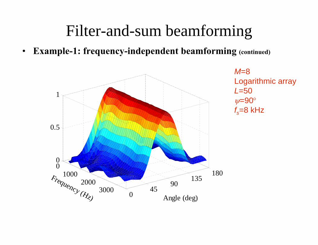
Filter-and-sum beamforming• Example-1: frequency-independent beamforming (continued)
M=8Logarithmic arrayL=50ψ=90°fs=8 kHz
01000
20003000 0
4590
135180
0
0.5
1
Angle (deg)
Frequency (Hz)

Filter-and-sum beamforming
• Example-2: `superdirective’ beamforming– Maximize directivity for known (diffuse) noise fields– Maximum directivity =M 2 obtained for diffuse noise & endfire steering (θ =0o)
Design: find F(ω) that maximizesfor given steering angle theta_max
– Optimal solution is
– This is equivalent to minimization of noise output power, subject to unit response for steering angle (**)
PS: Delay-and-sum beamformer similarly maximizes WNG
),()()( max1 θωωαω dΓF ⋅⋅= −
NN
1),()(s.t.),()()(min max)(=⋅⋅⋅ θωωωωω
ωdFFΓF
F
HNN
H
),()( maxθωαω dF ⋅=
(ΓNN = Ι)
)()()(),()(
)(2
max
ωωω
θωωω
FΓFdF
⋅⋅
⋅= diffuse
NNH
H
DI

• Example-2: `superdirective’ beamforming (continued)
Directivity patterns for endfire steering:
Superdirective beamformer has highest DI, but very poor WNGhence problems with robustness (e.g. sensor noise) !
Filter-and-sum beamforming
-20
-10
0
90
270
180 0
S u p e rd ire c tive b e a m fo rm e r (f=3 0 0 0 H z)
-20
-10
0
90
270
180 0
D elay-and-sum beamformer (f=3000 Hz)
M=5 d=3 cmtheta_max=0°fs=16 kHz
0 2 0 0 0 4 0 0 0 6 0 0 0 8 0 0 00
5
1 0
1 5
2 0
2 5
F re q u e n c y (H z )
Dire
ctiv
ity (l
inea
r)
S u p e rd i re c t iv eD e la y -a n d -s u m
0 2 0 0 0 4 0 0 0 6 0 0 0 8 0 0 0-6 0
-5 0
-4 0
-3 0
-2 0
-1 0
0
1 0
F re q u e n c y (H z )
Whi
te n
oise
gai
n (d
B)
S u p e rd i re c t iv eD e la y -a n d -s u m
6.99=10.Log(5)M 2
PS: diffuse noise =white noise for high frequencies

• Adaptive filter-and-sum structure:– Aim is to minimize noise output power, while maintaining a chosen frequency
response in a given look direction (and/or other linear constraints, see below)– This corresponds to operation of a superdirective array (see (**) p25), but now
noise field is unknown– Implemented as adaptive filter (e.g. constrained LMS algorithm)– Notation:
LCMV-beamforming
][kyM
][2 ky
][1 ky][1 kf
][2 kf
][kf M
Σ][kz Speaker
Noise ∑=
==M
mm
Tm
T kkkz1
][][][ yfyf
[ ]TTM
TT kkkk ][][][][ 21 yyyy K=
[ ]Tmmmm Lkykykyk ]1[]1[][][ +−−= Ky
[ ]TTM
TT ffff K21=
[ ]Tmmmm Lfff ]1[]1[]0[ −= Kf

LCMV = Linearly Constrained Minimum Variance– f designed to minimize variance of output z[k] :
– to avoid desired signal distortion/cancellation, add linear constraints:
– if noise and speech are uncorrelated, constrained output power minimization corresponds to constrained noise power minimization
– Type of constraints:• Frequency response in look-direction. Ex: (for broadside)
• Point, line and derivative constraints (=L constraints)
– Solution is (obtained using Lagrange-multipliers, etc..):
LCMV-beamforming
{ } fRfff
⋅⋅= ][min][min 2 kkzE yyT
JJMLT ℜ∈ℜ∈=⋅ × bCbfC ,with,
( ) bCRCCRf 111 ][][ −−− ⋅⋅⋅⋅= kk yyT
yyopt
∑=
=M
mm zF
11)(
Related Documents