Preamble OBL 302 Statistics What seems to be the problems? Students’ view OBL 302 Lecture 1-3 S.M.S. Massomo 1 Enhanced Face to Face Dec 2009 Mpwapwa

Preamble
Dec 30, 2015
Preamble. OBL 302 Statistics What seems to be the problems? Students’ view. Observations from the course tutor. It seems that some of you DO NOT know; How to use a scientific calculator for retrieval of mean, sum of squares, standard deviation etc. - PowerPoint PPT Presentation
Welcome message from author
This document is posted to help you gain knowledge. Please leave a comment to let me know what you think about it! Share it to your friends and learn new things together.
Transcript

Preamble
OBL 302 StatisticsWhat seems to be the problems?Students’ view
OBL 302Lecture 1-3
S.M.S. Massomo1
Enhanced Face to Face Dec 2009Mpwapwa

Observations from the course tutor
It seems that some of you DO NOT know;1. How to use a scientific calculator for retrieval of mean, sum of squares,
standard deviation etc. 2. Which test should be used for a particular situation (question?). 3. How to do simple calculations, hence you fail to arrive at the correct answer
even when you know the correct procedure 4. That in hypothesis testing you can not arrive at a conclusion without
comparing the value of the test statistic and the critical value that must be read from a specific/appropriate table (you are allowed to bring statistical tables in examination rooms)
INFACT many students do not know how to read tables to obtain critical values and hence fail to make correct conclusion(s) when
answering questions.
OBL 302Lecture 1-3
S.M.S. Massomo2
Enhanced Face to Face Dec 2009Mpwapwa
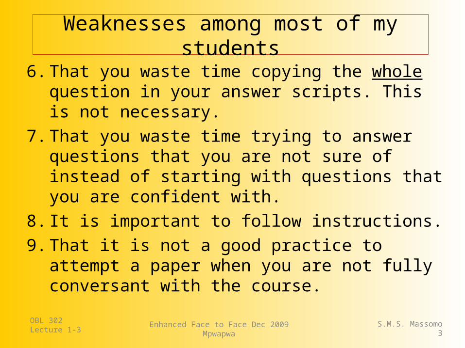
Weaknesses among most of my students
6. That you waste time copying the whole question in your answer scripts. This is not necessary.
7. That you waste time trying to answer questions that you are not sure of instead of starting with questions that you are confident with.
8. It is important to follow instructions. 9. That it is not a good practice to attempt a paper
when you are not fully conversant with the course.
OBL 302Lecture 1-3
S.M.S. Massomo3
Enhanced Face to Face Dec 2009Mpwapwa

OBL 302Lecture 1-3
S.M.S. Massomo4
Enhanced Face to Face Dec 2009Mpwapwa
You are advised to
Read as many as possible references including those in the internet, do not rely solely on the course outline.
Read other Open University of Tanzania study materials that are similar to the OBL302 course outline? For example;
Course code
Course name Target students
OED 215 Educational statistics Education OEC 123 Introduction to Statistics and
Mathematics for Economists BA Economics
OMT 153 Probability and statistics Mathematics OMT 254 Advanced Statistics, Design and
Analysis of Experiments Mathematics
OHE 352 Statistics and Research Methods for Home Economics
Home Economics

OBL 302Lecture 1-3
S.M.S. Massomo5
Enhanced Face to Face Dec 2009Mpwapwa
Use the internet: Do not be shy.
Form discussion groups, do not study alone
Ask for help
Use our web based OBL302 discussion forum or contact me by email to [email protected]
o Do a lot of exercises, you can start with the past paper questions, textbook examples and so on.
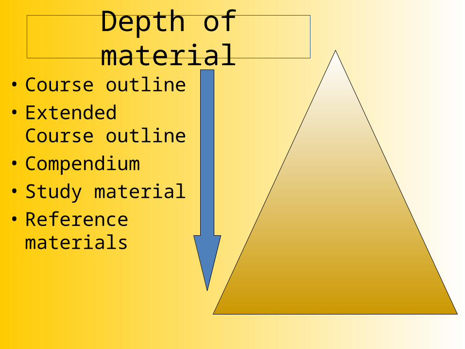
Depth of material
• Course outline• Extended Course
outline• Compendium• Study material• Reference materials

OBL 302 Biostatistics
Dr Said M.S. MassomoFSTES, Morogoro
OBL 302Lecture 1-3
Enhanced Face to Face Dec 2009Mpwapwa
S.M.S. Massomo7

1.0 Introduction
OBL 302Lecture 1-3
S.M.S. Massomo8
What is statistics?
• There are two meanings
2. A branch of science within applied mathematics that deals with a collection of methods/techniques for Planning experiments, Collecting data, and then Organising, Summarizing, Presenting, Analysing, Interpreting data so as to assist in making more effective decisions
1. Numerical informationSingular form Statistic, Collection of > one figure = statistics

Introduction cont..
S.M.S. Massomo9
Statistics?
• Taught as core course in most programmes (examples at the OUT)
• The main difference is on scope of coverage and examples used
• It is applied Mathematics, basic knowledge of simple algebra is sufficient to master the course
Introduction cont..
OBL 302Lecture 1-3
Enhanced Face to Face Dec 2009 Mpwapwa
S.M.S. Massomo10
Why study Statistics?
• Numerical information is everywhere, how do we determine if the conclusions determined are reasonable?
• Decisions affect our daily lives and personal welfare eg Drugs and appropriate dosage
• Understand why decisions are made and will give you a better understanding of how they affect you

Introduction cont..
OBL 302Lecture 1-3
S.M.S. Massomo11
• You will always be required to make informed decisions. The questions will be
• Is the information adequate or not• Will additional information, if it is needed, provide
results that are not misleading• How do you summarise the information in a useful and
informative way• How do you analyze the information• How to draw conclusions and make inferences while
assessing the risks of an incorrect conclusion
Introduction cont..
OBL 302Lecture 1-3
S.M.S. Massomo12
• Biostatistics: Also known as Biometry, refers to the application of statistics to solve biological problems
What is an experiment?
• Planned enquiry/activity designed with the aim of getting new information, confirm or deny certain previous information
Course Coverage
OBL 302Lecture 1-3
Enhanced Face to Face Dec 2009Mpwapwa
S.M.S. Massomo13
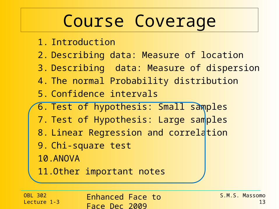
1. Introduction
2. Describing data: Measure of location
3. Describing data: Measure of dispersion
4. The normal Probability distribution
5. Confidence intervals
6. Test of hypothesis: Small samples
7. Test of Hypothesis: Large samples
8. Linear Regression and correlation
9. Chi-square test
10. ANOVA
11. Other important notes

Types of Statistics
OBL 302Lecture 1-3
S.M.S. Massomo14
There are two types of statistics (i) Descriptive statistics and
(ii) Inferential statistics
• Planning experiments,
• Collecting data,
• Organising data,
• Summarizing data,
• Presenting data,
• Analysing data,
• Interpreting data
• Conclusions
Descriptive statistics
Inferential statistics
Introduction cont..
OBL 302Lecture 1-3
S.M.S. Massomo15
Descriptive statistics: Are statistical procedures that describe, organise and summarize the main characteristics of sample data
• Organising data, How?• Summarizing data, how?
– Means, range Standard deviations, Frequency tables etc
• Presenting data, – Histograms, charts & tables etc

Introduction cont..
OBL 302Lecture 1-3
S.M.S. Massomo16
Standard Deviation & Standard error of the mean
• Calculations
• Short cut method
• Use of scientific calculators
• Implications
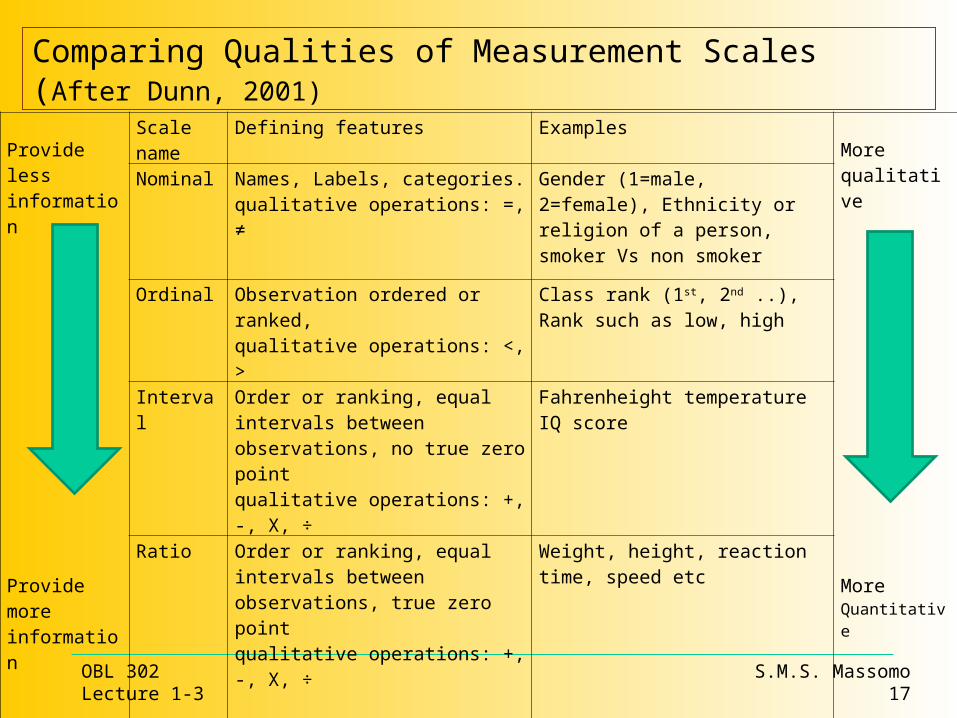
Comparing Qualities of Measurement Scales (After Dunn, 2001)
OBL 302Lecture 1-3
S.M.S. Massomo17
Provide less information
Provide more information
Scale name
Defining features ExamplesMore qualitative
More Quantitative
Nominal Names, Labels, categories. qualitative operations: =, ≠
Gender (1=male, 2=female), Ethnicity or religion of a person, smoker Vs non smoker
Ordinal Observation ordered or ranked,qualitative operations: <, >
Class rank (1st, 2nd ..), Rank such as low, high
Interval Order or ranking, equal intervals between observations, no true zero pointqualitative operations: +, -, X, ÷
Fahrenheight temperatureIQ score
Ratio Order or ranking, equal intervals between observations, true zero pointqualitative operations: +, -, X, ÷
Weight, height, reaction time, speed etc

Normal Probabilities
OBL 302Lecture 1-3
S.M.S. Massomo18
• Comprehension of this table is vital to success in the course!
• There is a table which must be used to look up standard normal probabilities. The z-score is broken into two parts, the whole number and tenth are looked up along the left side and the hundredth is looked up across the top. The value in the intersection of the row and column is the area under the curve between zero and the z-score looked up.
• Because of the symmetry of the normal distribution, look up the absolute value of any z-score.

Normal Probabilities
OBL 302Lecture 1-3
S.M.S. Massomo19
• There are several different situations that can arise when asked to find normal probabilities.
Situation I nstructions
Between zero and any number
Look up the area in the table
Between two positives, or Between two negatives
Look up both areas in the table and subtract the smaller from the larger.
Between a negative and a positive
Look up both areas in the table and add them together
Less than a negative, or Greater than a positive
Look up the area in the table and subtract from 0.5000
Greater than a negative, or Less than a positive
Look up the area in the table and add to 0.5000
Normal Probabilities
OBL 302Lecture 1-3
S.M.S. Massomo20
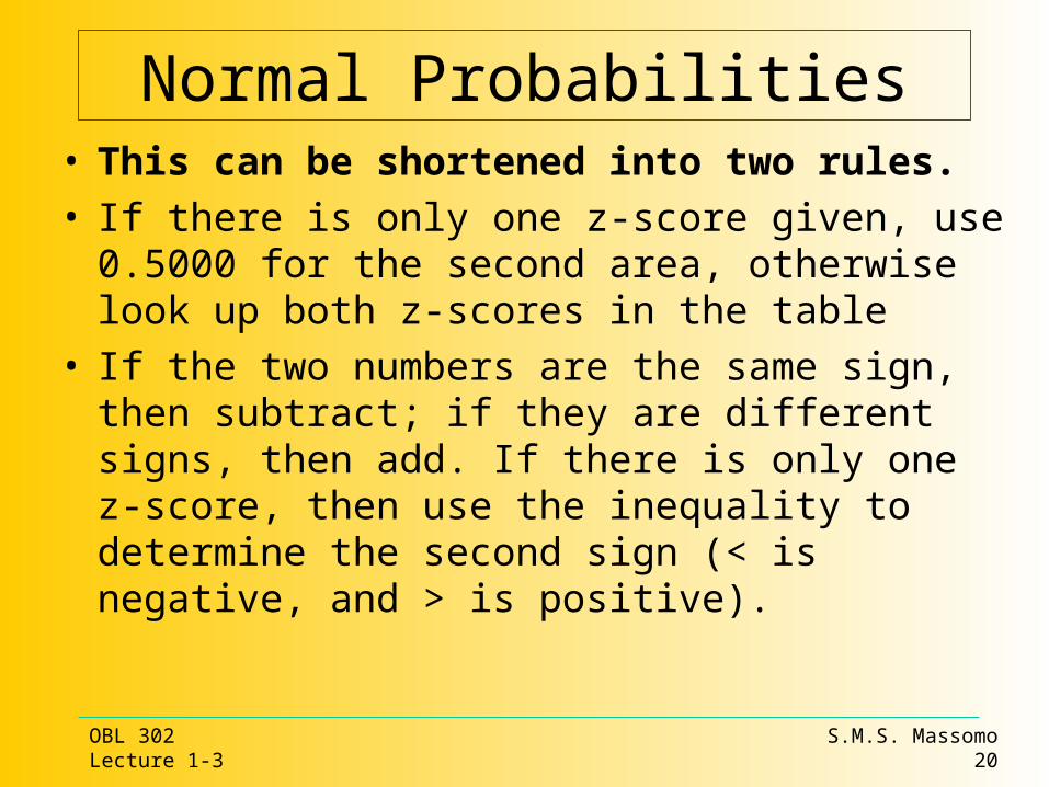
• This can be shortened into two rules. • If there is only one z-score given, use 0.5000 for the
second area, otherwise look up both z-scores in the table
• If the two numbers are the same sign, then subtract; if they are different signs, then add. If there is only one z-score, then use the inequality to determine the second sign (< is negative, and > is positive).
Normal Probabilities
OBL 302Lecture 1-3
S.M.S. Massomo21
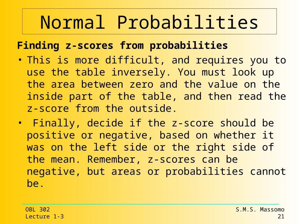
Finding z-scores from probabilities• This is more difficult, and requires you to use the table
inversely. You must look up the area between zero and the value on the inside part of the table, and then read the z-score from the outside.
• Finally, decide if the z-score should be positive or negative, based on whether it was on the left side or the right side of the mean. Remember, z-scores can be negative, but areas or probabilities cannot be.
Normal Probabilities
OBL 302Lecture 1-3
Enhanced Face to Face Dec 2009Mpwapwa
S.M.S. Massomo22
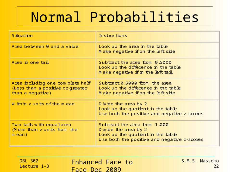
Situation Instructions
Area between 0 and a value Look up the area in the table Make negative if on the left side
Area in one tail Subtract the area from 0.5000 Look up the difference in the table Make negative if in the left tail
Area including one complete half (Less than a positive or greater than a negative)
Subtract 0.5000 from the area Look up the difference in the table Make negative if on the left side
Within z units of the mean Divide the area by 2 Look up the quotient in the table Use both the positive and negative z-scores
Two tails with equal area (More than z units from the mean)
Subtract the area from 1.000 Divide the area by 2 Look up the quotient in the table Use both the positive and negative z-scores

The Normal Probabilities..
OBL 302Lecture 1-3
Enhanced Face to Face Dec 2009Mpwapwa
S.M.S. Massomo23
• The values in the table are the areas between zero and the z-score.
• That is, P(0 < Z < z-score)
• See tables

OBL 302Lecture 1-3
Enhanced Face to Face Dec 2009Mpwapwa
S.M.S. Massomo24
Standard Normal Probabilities (Area under normal curve)
z 0.00 0.01 0.02 0.03 0.04 0.05 0.06 0.07 0.08 0.09
0.0 0.0000 0.0040 0.0080 0.0120 0.0160 0.0199 0.0239 0.0279 0.0319 0.0359
0.1 0.0398 0.0438 0.0478 0.0517 0.0557 0.0596 0.0636 0.0675 0.0714 0.0753
0.2 0.0793 0.0832 0.0871 0.0910 0.0948 0.0987 0.1026 0.1064 0.1103 0.1141
0.3 0.1179 0.1217 0.1255 0.1293 0.1331 0.1368 0.1406 0.1443 0.1480 0.1517
0.4 0.1554 0.1591 0.1628 0.1664 0.1700 0.1736 0.1772 0.1808 0.1844 0.1879
0.5 0.1915 0.1950 0.1985 0.2019 0.2054 0.2088 0.2123 0.2157 0.2190 0.2224
0.6 0.2257 0.2291 0.2324 0.2357 0.2389 0.2422 0.2454 0.2486 0.2517 0.2549
0.7 0.2580 0.2611 0.2642 0.2673 0.2704 0.2734 0.2764 0.2794 0.2823 0.2852
0.8 0.2881 0.2910 0.2939 0.2967 0.2995 0.3023 0.3051 0.3078 0.3106 0.3133
0.9 0.3159 0.3186 0.3212 0.3238 0.3264 0.3289 0.3315 0.3340 0.3365 0.3389
1.0 0.3413 0.3438 0.3461 0.3485 0.3508 0.3531 0.3554 0.3577 0.3599 0.3621
1.1 0.3643 0.3665 0.3686 0.3708 0.3729 0.3749 0.3770 0.3790 0.3810 0.3830
1.2 0.3849 0.3869 0.3888 0.3907 0.3925 0.3944 0.3962 0.3980 0.3997 0.4015
1.3 0.4032 0.4049 0.4066 0.4082 0.4099 0.4115 0.4131 0.4147 0.4162 0.4177

OBL 302Lecture 1-3
Enhanced Face to Face Dec 2009Mpwapwa
S.M.S. Massomo25
z 0.00 0.01 0.02 0.03 0.04 0.05 0.06 0.07 0.08 0.09
1.3 0.4032 0.4049 0.4066 0.4082 0.4099 0.4115 0.4131 0.4147 0.4162 0.4177
1.4 0.4192 0.4207 0.4222 0.4236 0.4251 0.4265 0.4279 0.4292 0.4306 0.4319
1.5 0.4332 0.4345 0.4357 0.4370 0.4382 0.4394 0.4406 0.4418 0.4429 0.4441
1.6 0.4452 0.4463 0.4474 0.4484 0.4495 0.4505 0.4515 0.4525 0.4535 0.4545
1.7 0.4554 0.4564 0.4573 0.4582 0.4591 0.4599 0.4608 0.4616 0.4625 0.4633
1.8 0.4641 0.4649 0.4656 0.4664 0.4671 0.4678 0.4686 0.4693 0.4699 0.4706
1.9 0.4713 0.4719 0.4726 0.4732 0.4738 0.4744 0.4750 0.4756 0.4761 0.4767
2.0 0.4772 0.4778 0.4783 0.4788 0.4793 0.4798 0.4803 0.4808 0.4812 0.4817
2.1 0.4821 0.4826 0.4830 0.4834 0.4838 0.4842 0.4846 0.4850 0.4854 0.4857
2.2 0.4861 0.4864 0.4868 0.4871 0.4875 0.4878 0.4881 0.4884 0.4887 0.4890
2.3 0.4893 0.4896 0.4898 0.4901 0.4904 0.4906 0.4909 0.4911 0.4913 0.4916
2.4 0.4918 0.4920 0.4922 0.4925 0.4927 0.4929 0.4931 0.4932 0.4934 0.4936
2.5 0.4938 0.4940 0.4941 0.4943 0.4945 0.4946 0.4948 0.4949 0.4951 0.4952
2.6 0.4953 0.4955 0.4956 0.4957 0.4959 0.4960 0.4961 0.4962 0.4963 0.4964
2.7 0.4965 0.4966 0.4967 0.4968 0.4969 0.4970 0.4971 0.4972 0.4973 0.4974
2.8 0.4974 0.4975 0.4976 0.4977 0.4977 0.4978 0.4979 0.4979 0.4980 0.4981
2.9 0.4981 0.4982 0.4982 0.4983 0.4984 0.4984 0.4985 0.4985 0.4986 0.4986
3.0 0.4987 0.4987 0.4987 0.4988 0.4988 0.4989 0.4989 0.4989 0.4990 0.4990


Inferential statistics
OBL 302Lecture 1-3
Enhanced Face to Face Dec 2009Mpwapwa
S.M.S. Massomo27
Inferential statistics: extend the scope of descriptive statistics by examining the relationships within a set of data, in particular, inferential statistics enable the researcher to make inference, that is conclusions / deductions / judgements, about the population based on the relationships within the sample data.
Inferential statistics: Unlike descriptive statistics, inferential statistics make inference about a population basing on sample data
Population Vs Sample
OBL 302Lecture 1-3
Enhanced Face to Face Dec 2009Mpwapwa
S.M.S. Massomo28
• Population: All subjects possessing a common characteristic that is being studied. Example?
• Sample: subgroup or subset of the population. examples?
• Why do we work with samples?

Inferential Statistics
OBL 302Lecture 1-3
Enhanced Face to Face Dec 2009Mpwapwa
S.M.S. Massomo29
Why do we work with samples?
1. Cost
2. Practicability, eg destructive sampling
3. Time constraint
4. It is possible to draw correct conclusions if sampling is done in a proper way

Inferential statistics...
OBL 302Lecture 1-3
Enhanced Face to Face Dec 2009Mpwapwa
S.M.S. Massomo30
• Random sample: A sample that has been drawn from a population such that each individual in the population has an equal chance of being selected.
• Central limit theorem: theorem which states ‘as the sample size increases, the sampling distribution of the sample means will become approximate normally distributed
• Sampling error: Difference that occurs between the sample statistic and the population parameter due to the fact that the sample is not a perfect representation of the population.

Inferential statistics: Test of hypotheses
OBL 302Lecture 1-3
Enhanced Face to Face Dec 2009Mpwapwa
S.M.S. Massomo31
Test of hypotheses (Also called test of significance)
• Definition: It is a statistical test that examine a set of sample data, and on a basis of an expected distribution of the data (eg Z, t, F or Chi),at a specific level of significance and leads to a decision about whether to reject null hypothesis or alternative hypothesis

Test of hypotheses...
OBL 302Lecture 1-3
Enhanced Face to Face Dec 2009Mpwapwa
S.M.S. Massomo32
• Statistical tests = difference between sample means divided by Error term (within group error)
• Statistical significance: Refers to whether a test detected a reliable difference between two or more groups, one caused by the effect of an independent variable on a dependent measure
Test of hypotheses..
OBL 302Lecture 1-3
Enhanced Face to Face Dec 2009Mpwapwa
S.M.S. Massomo33
• A hypothesis: A statement about a population that is subject for testing. Hypothesis may be null or alternative.
• Null hypothesis: A statement about a population that is under test. Denoted as Ho, and Ho state that there is no difference between means or there is no effect. Always include the equal sign =,
• Alternative hypothesis: A statement that is true when Ho is false. Hi determine whether the test is left/right one tailed of two tailed. Characterised by presence of inequality sign
Test of hypotheses: Type I error and Type II error
OBL 302Lecture 1-3
Enhanced Face to Face Dec 2009Mpwapwa
S.M.S. Massomo34
Type I: Rejecting Ho when it is true. Usually more serious error
Type II: Accepting Ho when it is false, that is saying true when it is false (examples...).
• Usually defendants are presumed innocent until proven guilty. The purpose of a court trial is to see whether a null hypothesis of innocence is rejected by the weight of the data (evidence).
• The null hypothesis : Ho = the person is innocent,
• The alternative hypothesis Hi = the person is guilty
Which is more serious error? Convicting an innocent person or letting the guilty person go free?
Test of hypotheses...
OBL 302Lecture 1-3
Enhanced Face to Face Dec 2009Mpwapwa
S.M.S. Massomo35
Level of significance: Also called p-value or alpha. Refers to the probability of rejecting the null hypothesis when it is true. P=0.05 and 0.01 are common for biological studies. It is a way of expressing the likelihood that Ho is not true. The level of significance is the complement of the level of confidence in estimation. If no level of significance is given then use P=0.05.
Test statistic: A value, determined from sample information, used to determine whether to reject the null hypothesis. Eg Z, t, F value.
Test of hypotheses...
OBL 302Lecture 1-3
Enhanced Face to Face Dec 2009Mpwapwa
S.M.S. Massomo36
A critical value: The value(s) which separates the critical region from the non critical region.
• The critical values are determined independently of the sample statistics.
• They are read from appropriate tables of distribution.
Critical region: also called rejection region, is a set of all values which would cause us to reject Ho. If the test statistic falls in the rejection region Ho is rejected.
Test of hypotheses...
OBL 302Lecture 1-3
Enhanced Face to Face Dec 2009Mpwapwa
S.M.S. Massomo37
Arrive at a decision: A statement based upon the null hypothesis. It is either ‘reject the null hypothesis’ or ‘fail to reject the null hypothesis’. Usually we NEVER accept the null hypothesis.
Conclusion: A statement which indicates the level of evidence (sufficient or insufficient), at a specific level of significance and decide whether the original claim is rejected (null) or supported (alternative)

Coverage OBL 302 part II1. Test of hypothesis: Small samples using t test
a) The t test for small samplesb) The t test for independent samplesc) The t test for dependent samples
2. Test of Hypothesis: Large samples using Z test3. Chi-square test4. Linear Regression and correlation5. ANOVA6. Other important notes
OBL 302Lecture 1-3
S.M.S. Massomo38
Enhanced Face to Face Dec 2009Mpwapwa

Test of hypothesesSmall samples using the t test
Why use t distribution?The t-test is used for small samples (n < 30) as Z
distribution provides unreliable estimates of differences between samples when the number of available observation is less than 30
Remember the t distribution is more flatter than the Z distribution
OBL 302Lecture 1-3
S.M.S. Massomo39
Enhanced Face to Face Dec 2009Mpwapwa
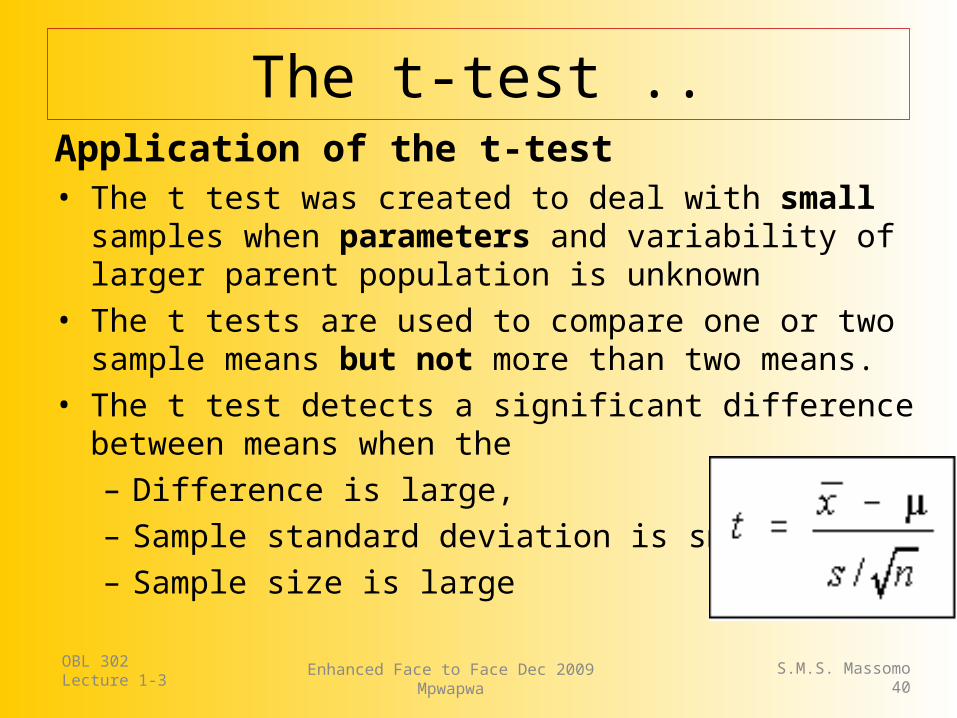
The t-test ..Application of the t-test• The t test was created to deal with small samples when
parameters and variability of larger parent population is unknown
• The t tests are used to compare one or two sample means but not more than two means.
• The t test detects a significant difference between means when the– Difference is large, – Sample standard deviation is small and or – Sample size is large
OBL 302Lecture 1-3
S.M.S. Massomo40
Enhanced Face to Face Dec 2009Mpwapwa
Variation of the t test: 1. Single or one sample t test
• This is used to compare the observed mean of one sample with a hypothesized value assumed to represent a population.
• T or Z test both use similar formulasTest statistic= Diference between sample means
Standard error of the mean• It tries to answer the question: is it likely that a sample with a
given mean could have come from a population with the proposed µ?
• It is usually used to determine if some set of scores or observation deviate from some established pattern examples?
OBL 302Lecture 1-3
S.M.S. Massomo41
Enhanced Face to Face Dec 2009Mpwapwa
Variation of the t test: 1. Single or one sample t test
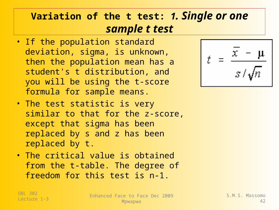
• If the population standard deviation, sigma, is unknown, then the population mean has a student's t distribution, and you will be using the t-score formula for sample means.
• The test statistic is very similar to that for the z-score, except that sigma has been replaced by s and z has been replaced by t.
• The critical value is obtained from the t-table. The degree of freedom for this test is n-1.
OBL 302Lecture 1-3
S.M.S. Massomo42
Enhanced Face to Face Dec 2009Mpwapwa
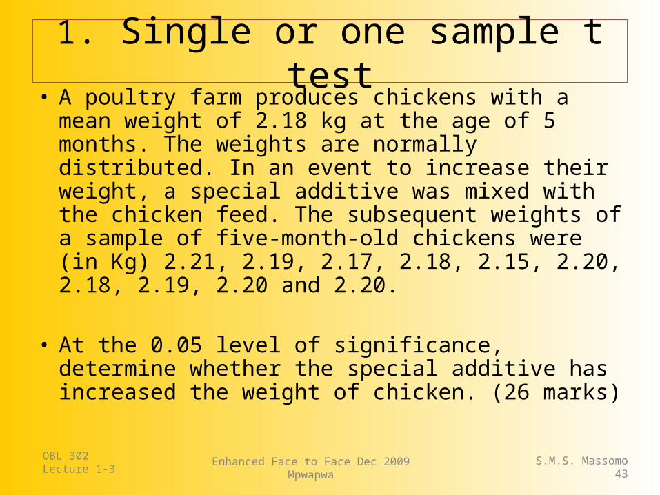
1. Single or one sample t test• A poultry farm produces chickens with a mean weight
of 2.18 kg at the age of 5 months. The weights are normally distributed. In an event to increase their weight, a special additive was mixed with the chicken feed. The subsequent weights of a sample of five-month-old chickens were (in Kg) 2.21, 2.19, 2.17, 2.18, 2.15, 2.20, 2.18, 2.19, 2.20 and 2.20.
• At the 0.05 level of significance, determine whether the special additive has increased the weight of chicken. (26 marks)
OBL 302Lecture 1-3
S.M.S. Massomo43
Enhanced Face to Face Dec 2009Mpwapwa

1. Single or one sample t test
OBL 302Lecture 1-3
S.M.S. Massomo44
Enhanced Face to Face Dec 2009Mpwapwa
Step 1. Calculate the sample Standard deviation and Mean
Sd =ටσ𝑥2−(σ𝑥)2 𝑛ൗ�𝑛−1
ඩ47.25−ሺ21.87ሻ2 10൘
10−1 = ට47.25−478.30 10ൗ�9 = ට47.25−47.839 =
𝑠𝑑= ξ0.05 = 0.0177
Mean (x) = σ𝑥/𝑛 = 21.87/10 = 𝟐.𝟏𝟖𝟕
Variation of the t test: 1. Single or one sample t test
OBL 302Lecture 1-3
S.M.S. Massomo45
Enhanced Face to Face Dec 2009Mpwapwa
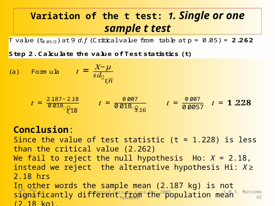
T value (t0.05/2) at 9 d.f (Critical value from table at p = 0.05) = 2.262
Step 2. Calculate the value of Test statistics (t)
(a) Formula 𝑡 = 𝑋−µ𝑠𝑑 ξ𝑛൘
𝑡 = 2.187−2.180.018 ξ10ൗ� 𝑡 = 0.0070.018 3.16ൗ�
𝑡 = 0.0070.0057 𝑡 = 𝟏.𝟐𝟐𝟖
Conclusion: Since the value of test statistic (t = 1.228) is less than the critical value (2.262)We fail to reject the null hypothesis Ho: X = 2.18, instead we reject the alternative hypothesis Hi: X ≥ 2.18 hrsIn other words the sample mean (2.187 kg) is not significantly different from the population mean (2.18 kg).
2. The T test for independent groups (two sample test)
• Independent Samples: samples are independent when they are not related.
• Independent samples may or may not have the same sample size.
• Designed to detect significant difference between a control group and an experimental group
• It tries to answer the Question: Is X1 different from X2 or could the two sample means come from identical population?
• Examples....see Z test for two samples why?• The test statistic is very similar to that for the z-score, except
that sigma has been replaced by s and z has been replaced by t. OBL 302Lecture 1-3
S.M.S. Massomo46
Enhanced Face to Face Dec 2009Mpwapwa

3. Dependent Samples T test (paired samples t test)
• Samples in which the subjects are paired or matched in some way
• Dependent samples must have the same sample size, but it is possible to have the same sample size without being dependent.
Type of Dependent samples are • Those characterised by a measurement, an intervention of some
type, then another measurement. In other words, a paired t test is designed to detect the presence of measurable change in the average attitude/behaviour of group from one point in time to another point in time.
It tries to answer the Question: Is the mean one (X1) different from mean two (X2)?
• Involves matching or pairing of observation
OBL 302Lecture 1-3
S.M.S. Massomo47
Enhanced Face to Face Dec 2009Mpwapwa

The t test: Dependent samples
OBL 302Lecture 1-3
S.M.S. Massomo48
Enhanced Face to Face Dec 2009Mpwapwa
To measure the effect of a fitness campaign, five students were randomly sampled and their weights (in Kg) were recorded before and after the exercise as presented in the following table. Using 0.05 level of significance, determine whether the campaign had any significantly effect on the students (18 marks).
Students A B C D E Before 88.45 76.65 83.00 70.30 76.20 After 89.35 73.93 81.65 68.04 72.57
...... characterised by a measurement, an intervention of some type, then another measurement. In other words, a paired t test is designed to detect the presence of measurable change in the average attitude/behaviour of group from one point in time to another point in time.

The t test: Dependent samples
OBL 302Lecture 1-3
S.M.S. Massomo49
Enhanced Face to Face Dec 2009Mpwapwa
Student Before After d d2 A 88.45 89.35 -0.90 0.81 B 76.65 73.93 2.72 7.40 C 83.00 81.65 1.35 1.82 D 70.30 68.04 2.26 5.11 E 76.20 72.57 3.63 13.18
Total 9.06 28.32
Mean
1.81

The t test: Dependent samples
OBL 302Lecture 1-3
S.M.S. Massomo50
Enhanced Face to Face Dec 2009Mpwapwa
SD = = = =
= 1.73
Formula t = = = = =
2 marks for SD formula
4 marks for SD value
2 marks for table t value
3 marks for correct conclusion
2 marks for t formula
2 marks for t value
2.35
The t test: Dependent samples
OBL 302Lecture 1-3
S.M.S. Massomo51
Enhanced Face to Face Dec 2009Mpwapwa
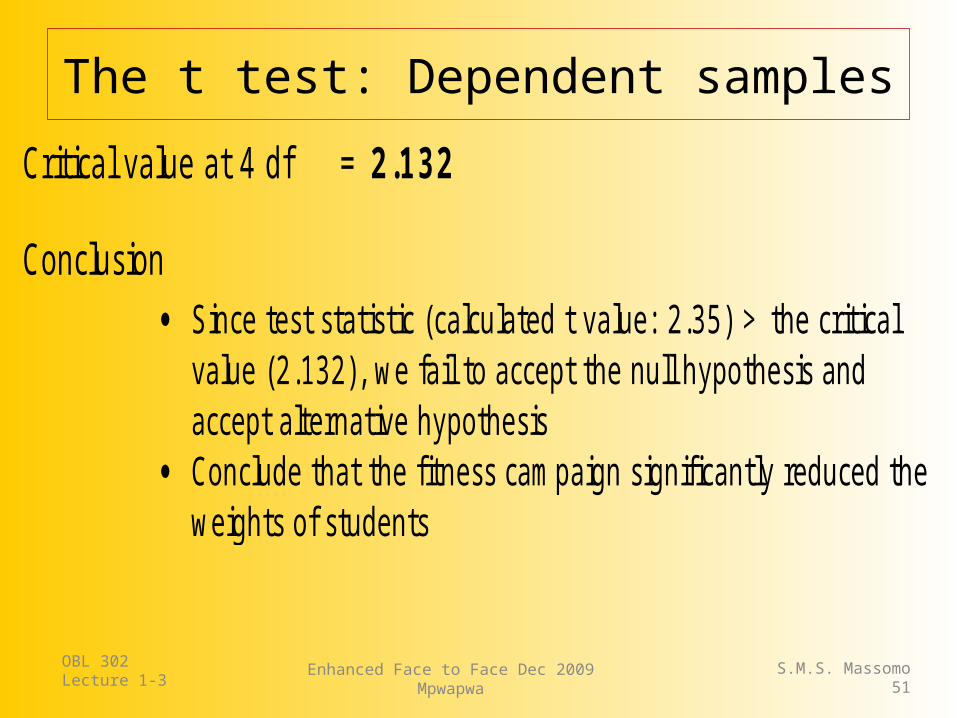
Critical value at 4 df = 2.132
Conclusion Since test statistic (calculated t value: 2.35) > the critical
value (2.132), we fail to accept the null hypothesis and accept alternative hypothesis
Conclude that the fitness campaign significantly reduced the weights of students

OBL 302Lecture 1-3
S.M.S. Massomo52
Enhanced Face to Face Dec 2009Mpwapwa

The Z test: one sampleQ3. A manufacturing process has produced
thousands units of a certain laboratory chemical with a mean shelf life of 1,200 hours and a standard deviation of 300 hours. A new process is tried and a sample of 100 units produced had a sample average of 1,265 hours.
• At the 0.05 level of significance, determine whether the new manufacturing process is better than the old one (18 marks)
• Is this a one tailed test or two tailed test? Why? (7 marks).
OBL 302Lecture 1-3
S.M.S. Massomo53
Enhanced Face to Face Dec 2009Mpwapwa

The Z test:one sample
OBL 302Lecture 1-3
S.M.S. Massomo54
Enhanced Face to Face Dec 2009Mpwapwa
(a) Formula
Critical value from table at p = 0.05 is 1.96
Conclusion: Since the value of test statistic (Z=2.167) exceed the critical value (1.96)
We fail to accept null hypothesis Ho: µ = 1200 hrs and accept the alternative hypothesis Hi: µ ≥ 1200 hrs
In other words the sample mean (1265 hrs) is significantly greater than the population mean (1200 hrs).
2 marks for Z formula
6 marks for Z value
5 marks for table value
5 marks for correct conclusion

The Z test: one sample
OBL 302Lecture 1-3
S.M.S. Massomo55
Enhanced Face to Face Dec 2009Mpwapwa
(b) This is a one tailed test (3 marks)
Why? Because the intention of the study and was to improve the process of production and Hi show a directional increase (4 marks)

The Z test: two sample• A random sample of 120 workers in one large farm
took an average of 22.0 minutes to complete a task, with a variance of 4. A random sample of 120 workers in a second large plant took an average of 19.0 minutes to complete the task, with a variance of 10.
• Using an appropriate test, at the 5% level, Determine whether there is a significant difference between the two populations mean completion times (11 marks)
OBL 302Lecture 1-3
S.M.S. Massomo56
Enhanced Face to Face Dec 2009Mpwapwa
The Z test: two sample
OBL 302Lecture 1-3
S.M.S. Massomo57
Enhanced Face to Face Dec 2009Mpwapwa
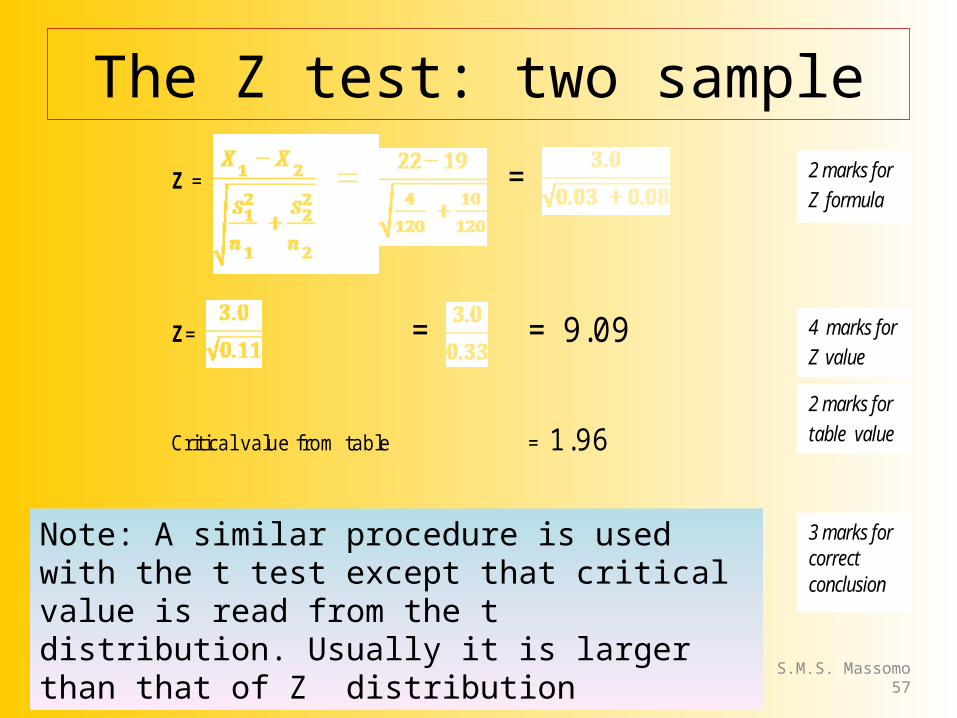
Z = =
Z= = = 9.09
Critical value from table = 1.96
2 marks for Z formula
4 marks for Z value
2 marks for table value
3 marks for correct conclusion
Note: A similar procedure is used with the t test except that critical value is read from the t distribution. Usually it is larger than that of Z distribution

The Z test: two sampleConclusion: • Since test statistic (calculated Z value: 9.09) > the
critical value (1.96), we fail to accept the null hypothesis and accept alternative hypothesis
• That is the two mean completion times are significantly different
OBL 302Lecture 1-3
S.M.S. Massomo58
Enhanced Face to Face Dec 2009Mpwapwa

The Z test: two sampleIs this a one tailed or two tailed test? Why? (4 marks)• It is a two tailed test (2 marks)• Because the intention was to find whether the two
means differ. Alternative hypothesis Hi: X1 ≠ X2 does not indicate a direction (2 marks)
• What is the p-value? (3 marks)• Since the test statistic (9.09) is far greater than max Z
value of 3.0 in the table, the p-value is less than 0.001. That is 0.5 – 0.4990
OBL 302Lecture 1-3
S.M.S. Massomo59
Enhanced Face to Face Dec 2009Mpwapwa

OBL 302Lecture 1-3
S.M.S. Massomo60
Enhanced Face to Face Dec 2009Mpwapwa

The Chi Square test: Definitions• Chi-square distribution : A distribution obtained from the multiplying
the ratio of sample variance to population variance by the degrees of freedom when random samples are selected from a normally distributed population
• Contingency Table : Data arranged in table form for the chi-square independence test
• Expected Frequency : The frequencies obtained by calculation. • Goodness-of-fit Test : A test to see if a sample comes from a
population with the given distribution. • Independence Test : A test to see if the row and column
variables are independent. • Observed Frequency: The frequencies obtained by observation.
These are the sample frequencies.
OBL 302Lecture 1-3
S.M.S. Massomo61
Enhanced Face to Face Dec 2009Mpwapwa
(χ2) Chi-square..Properties of the (χ2) Chi-square distribution are• Chi-square is non-negative. Is the ratio of two non-
negative values, therefore must be non-negative itself.
• Chi-square is non-symmetric. • There are many different chi-square distributions,
one for each degree of freedom. • The degrees of freedom when working with a
single population variance is n-1.
OBL 302Lecture 1-3
S.M.S. Massomo62
Enhanced Face to Face Dec 2009Mpwapwa

Application of the χ2 testApplication of the χ2 test 1. Goodness-of-fit Test2. Test for Independence
OBL 302Lecture 1-3
S.M.S. Massomo63
Enhanced Face to Face Dec 2009Mpwapwa
Variation of the χ2 test: 1. Goodness-of-fit Test
• The idea behind the chi-square goodness-of-fit test is to see if the sample comes from the population with the claimed distribution. Another way of looking at that is to ask if the frequency distribution fits a specific pattern.
• Two values are involved, an observed value, which is the frequency of a category from a sample, and the expected frequency, which is calculated based upon the claimed distribution.
• The idea is that if the observed frequency is really close to the claimed (expected) frequency, then the square of the deviations will be small.
OBL 302Lecture 1-3
S.M.S. Massomo64
Enhanced Face to Face Dec 2009Mpwapwa

Variation of the χ2 test: 1. Goodness-of-fit Test
QuestionAccording to the Mendelian genetic model, a certain garden pea plant should produce offspring that have white, pink, and red flowers, in the proportion of 25%, 50%, 25%. A sample of 1000 such offspring was coloured as follows: white 21%; red 27% ; pink 52%.
• Using an appropriate test, can you reject the Mendelian hypothesis at the 5% level? (25 marks).
OBL 302Lecture 1-3
S.M.S. Massomo65
Enhanced Face to Face Dec 2009Mpwapwa
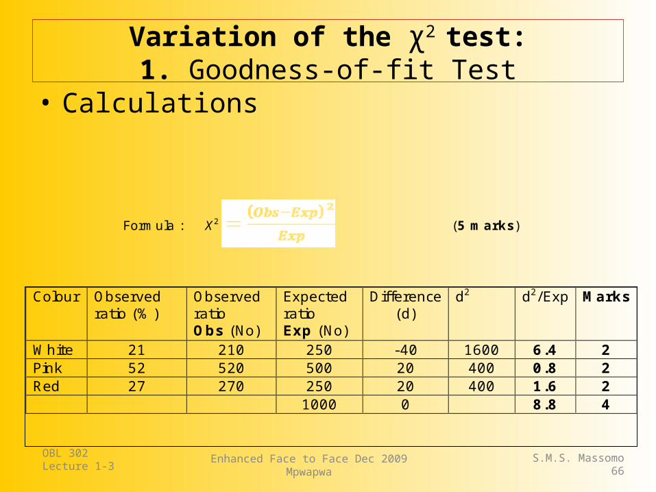
Variation of the χ2 test: 1. Goodness-of-fit Test
• Calculations
OBL 302Lecture 1-3
S.M.S. Massomo66
Enhanced Face to Face Dec 2009Mpwapwa
Colour Observed ratio (%)
Observed ratio Obs (No)
Expected ratio Exp (No)
Difference (d)
d2 d2/Exp Marks
White 21 210 250 -40 1600 6.4 2 Pink 52 520 500 20 400 0.8 2 Red 27 270 250 20 400 1.6 2 1000 0 8.8 4
Formula : X2 (5 marks)

Variation of the χ2 test: 1. Goodness-of-fit Test
• Calculated value = 8.8• X2 table value (critical value) at 0.05 = 5.991 (5 marks)• Conclusion: (5 marks)• Since calculated value (8.8), of the test statistic, is
greater than the critical value at 0.05 (5.991), we fail to accept null hypothesis (Ho) and accept null hypothesis (Hi), that is observed values significantly deviate from the expected 25:50:25 ratio
OBL 302Lecture 1-3
S.M.S. Massomo67
Enhanced Face to Face Dec 2009Mpwapwa
Variation of the χ2 test: 2. Test for independence
• In the test for independence, the claim is that the row and column variables are independent of each other. This is the null hypothesis.
• The multiplication rule said that if two events were independent, then the probability of both occurring was the product of the probabilities of each occurring.
• This is key to working the test for independence. If you end up rejecting the null hypothesis, then the assumption must have been wrong and the row and column variable are dependent. Remember, all hypothesis testing is done under the assumption the null hypothesis is true.
OBL 302Lecture 1-3
S.M.S. Massomo68
Enhanced Face to Face Dec 2009Mpwapwa
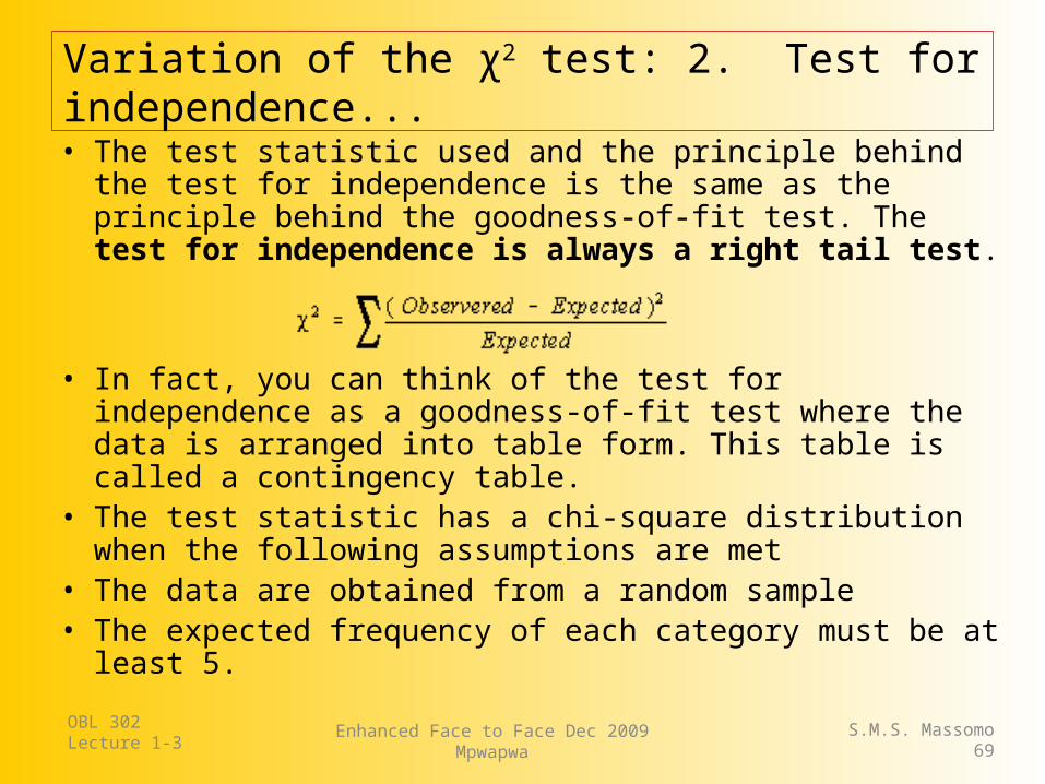
Variation of the χ2 test: 2. Test for independence...
• The test statistic used and the principle behind the test for independence is the same as the principle behind the goodness-of-fit test. The test for independence is always a right tail test.
• In fact, you can think of the test for independence as a goodness-of-fit test where the data is arranged into table form. This table is called a contingency table.
• The test statistic has a chi-square distribution when the following assumptions are met
• The data are obtained from a random sample • The expected frequency of each category must be at least 5.
OBL 302Lecture 1-3
S.M.S. Massomo69
Enhanced Face to Face Dec 2009Mpwapwa

Variation of the χ2 test: 2. Test for independence
OBL 302Lecture 1-3
S.M.S. Massomo70
Enhanced Face to Face Dec 2009Mpwapwa
An ecological study was carried out to determine the association between two plant species in Serengeti plains. The researchers randomly threw a 1m X 1m sampling frame several times and recoded the presence and or absence of the two plant species in the samples as follows;
Plant species A Plant species B Totals
Present Absent Present 90 (A) 181 (B) 271 Absent 66 (C) 113 (D) 179 Totals 156 294 450

Variation of the χ2 test: 2. Test for independence
What is random sampling? (give 6 marks)• Random sampling: Sampling that gives each individual
in the population a known likelihood/equal chance of being selected in the sample
• Extras: Avoid biasness and may result into a representative sample
Perform an appropriate test, using the 0.05 level of significance, to determine if there is association between the two species (14 marks)
OBL 302Lecture 1-3
S.M.S. Massomo71
Enhanced Face to Face Dec 2009Mpwapwa

Variation of the χ2 test: 2. Test for independence
OBL 302Lecture 1-3
S.M.S. Massomo72
Enhanced Face to Face Dec 2009Mpwapwa
Shortcut method
formula X2 =
≈ 0.639
Variation of the χ2 test: 2. Test for independence
OBL 302Lecture 1-3
S.M.S. Massomo73
Enhanced Face to Face Dec 2009Mpwapwa
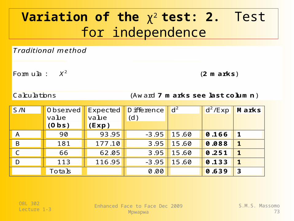
Traditional method
Formula : X2 (2 marks)
Calculations (Award 7 marks see last column)
S/N Observed value (Obs)
Expected value (Exp)
Difference (d)
d2 d2/Exp Marks
A 90 93.95 -3.95 15.60 0.166 1
B 181 177.10 3.95 15.60 0.088 1
C 66 62.05 3.95 15.60 0.251 1
D 113 116.95 -3.95 15.60 0.133 1
Totals 0.00 0.639 3

Variation of the χ2 test: 2. Test for independence
• Calculated X2 value (test statistic) = 0.639• X2 table value (critical value) at 0.05 =
3.841 (2 marks)
Conclusion: (3 marks)• Since calculated value (0.639), of the test statistic,
is less than the critical value at 0.05 (3.841), we do not reject the null hypothesis (Ho) and reject alternative hypothesis (Hi), and conclude there is no association between the two species
OBL 302Lecture 1-3
S.M.S. Massomo74
Enhanced Face to Face Dec 2009Mpwapwa
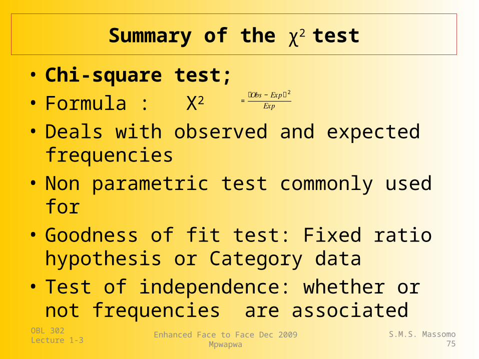
Summary of the χ2 test
• Chi-square test;• Formula : X2
• Deals with observed and expected frequencies• Non parametric test commonly used for • Goodness of fit test: Fixed ratio hypothesis or
Category data• Test of independence: whether or not frequencies
are associated
OBL 302Lecture 1-3
S.M.S. Massomo75
Enhanced Face to Face Dec 2009Mpwapwa
= ሺ𝑂𝑏𝑠− 𝐸𝑥𝑝ሻ2𝐸𝑥𝑝
Regression Analysis
OBL 302Lecture 1-3
S.M.S. Massomo76
Enhanced Face to Face Dec 2009Mpwapwa
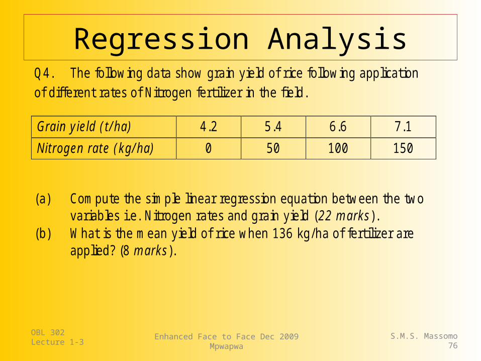
Q4. The following data show grain yield of rice following application of different rates of Nitrogen fertilizer in the field.
(a) Compute the simple linear regression equation between the two variables i.e. Nitrogen rates and grain yield (22 marks).
(b) What is the mean yield of rice when 136 kg/ha of fertilizer are applied? (8 marks).
Grain yield (t/ha) 4.2 5.4 6.6 7.1
Nitrogen rate (kg/ha) 0 50 100 150
Regression AnalysisRegression analysis; • A procedure used to predict the value of one dependent
variable (Y) from another independent variable (X) • Regression equation y = a + bxCorrelation analysis;• A test that determines the nature and strength of
association between two or more variables• Correlation can be zero, positive or negative• Diagram(s)
OBL 302Lecture 1-3
S.M.S. Massomo77
Enhanced Face to Face Dec 2009Mpwapwa

Correlation Analysis• Increase in one variable
result into a decrease of the other variable and vice versus
• This is an example of ......... Linear Correlation
OBL 302Lecture 1-3
S.M.S. Massomo78
Enhanced Face to Face Dec 2009Mpwapwa

Regression Analysis
OBL 302Lecture 1-3
S.M.S. Massomo79
Enhanced Face to Face Dec 2009Mpwapwa
X mean = 75 = 35,000
a = 4.33 b = 0.02 = 140.77
(a) Formula for b = =
0.0198 ≈ 0.02
Formula for a = = ≈
4.33
2 marks for b formula
6 marks for b value
6 marks for ‘a’ value
6 marks for correct Regression formula
2 marks for ‘a’ formula

Regression Analysis
OBL 302Lecture 1-3
S.M.S. Massomo80
Enhanced Face to Face Dec 2009Mpwapwa
Simple linear regression equation: (Y= a + bx) = Y = 4.33 + 0.02x
(b) Yield of rice when 136 kg/ha of fertilizer are applied? (8 marks, award 2 marks for the formula and 6 for correct answer).
Formula: Y= a + bx
Y = 4.33 + (0.02 x 136)
Y = 4.33 + 2.72 = 7.05 Kg

The F test• Test whether two samples are from a population
with equal variances• Comparison of several means simultaneously ANOVA
OBL 302Lecture 1-3
S.M.S. Massomo81
Enhanced Face to Face Dec 2009Mpwapwa

ANOVA• Analysis of variance;• Abbreviated as ANOVA, is a technique used to test
a hypothesis concerning means of three or more populations
• It determines if there is statistical differences between the means
• It is based on the F test that test whether two independent variances are equal or not
• It is a right tailed test• F distribution is used
OBL 302Lecture 1-3
S.M.S. Massomo82
Enhanced Face to Face Dec 2009Mpwapwa

ANOVA
OBL 302Lecture 1-3
S.M.S. Massomo83
Enhanced Face to Face Dec 2009Mpwapwa
Study the following yield data obtained from a certain fertilizer experiment. Prepare an ANOVA table and at the 0.05 level of significance, determine (i) Whether fertilizers differ and (ii) Whether replications differ (18 marks).
Fertilizer Applied
Replication Totals 1 2 3 4
No fertilizer 6.0 6.4 6.5 5.5 24.4 Fertilizer A 6.9 7.5 7.0 6.6 28.0 Fertilizer B 7.2 7.4 7.8 6.8 29.2 Totals 20.1 21.3 21.3 18.9 81.6

ANOVA
OBL 302Lecture 1-3
S.M.S. Massomo84
Enhanced Face to Face Dec 2009Mpwapwa
Study the following yield data obtained from a certain fertilizer experiment. Prepare an ANOVA table and at the 0.05 level of significance, determine (i) Whether fertilizers differ and (ii) Whether replications differ (18 marks).
Fertilizer Applied
Replication Totals 1 2 3 4
No fertilizer 6.0 6.4 6.5 5.5 24.4 Fertilizer A 6.9 7.5 7.0 6.6 28.0 Fertilizer B 7.2 7.4 7.8 6.8 29.2 Totals 20.1 21.3 21.3 18.9 81.6
= 81.6

ANOVA
OBL 302Lecture 1-3
S.M.S. Massomo85
Enhanced Face to Face Dec 2009Mpwapwa
Correction factor (CF) = = = 554.88 (1.5 marks)
Total SS = 559.56 – CF = 4.68
Rep SS = ((20.12 + ... 18.92) / 3) – CF , = (1668.60 / 3) – CF
= 556.2 – CF = 1.32
Treat SS = ((24.42 + 28.02 + 29.22) / 4) – CF , = (2232/4) – CF = 558.00 – CF = 3.12
Error SS = Total SS – (Rep SS + Treat SS)
= 4.68 – (1.32 + 31.2) = 0.24

ANOVA cont..
OBL 302Lecture 1-3
S.M.S. Massomo86
Enhanced Face to Face Dec 2009Mpwapwa
Source of variation
Degree of freedom
Sum of squares
Mean SS F-Value Table F-value (0.05)
Rep. 3 1.32 0.44 11.00 4.76 Treat. 2 3.12 1.56 39.00 5.14 Error 6 0.24 0.04 Total 11 4.68 Conclusions (4 marks: Award 2 marks for each correct conclusion) (i) Since calculated F value 11.0 (test statistic) for Replications > table value
4.76 (critical value) we fail to accept Ho. We accept Hi: and conclude that the means for replications differ significantly
(ii) Since calculated F value 39.0 (test statistic) for Treatments > table value 5.14 (critical value) we fail to accept Ho. We accept Hi: and conclude that the means for treatments/fertilizers differ significantly
Related Documents