Pre-Modeling Via BART

Pre-Modeling Via BART

Ed George, University of Pennsylvania (joint work with H. Chipman and R. McCulloch)

Tenth Annual Winter WorkshopBayesian Model Selection and Objective Methods

Department of StatisticsUniversity of FloridaJanuary 11-12, 2008

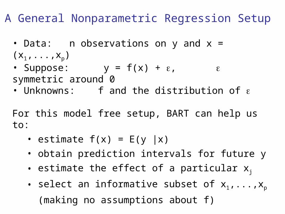
• Data: n observations on y and x = (x1,...,xp)• Suppose: y = f(x) + , symmetric around 0• Unknowns: f and the distribution of

For this model free setup, BART can help us to:

• estimate f(x) = E(y |x)

• obtain prediction intervals for future y

• estimate the effect of a particular xj

• select an informative subset of x1,...,xp

(making no assumptions about f)

Remark: In what follows we will assume ~ N(0, 2) for simplicity, but extension to a general DP process normal mixture model for works just fine.

A General Nonparametric Regression Setup

How Does BART Work?

x2 < d x2 d

x5 < c x5 c

= 7

= -2 = 5

BART (= Bayesian Additive Regression Trees) is composed of many single tree models

Let g(x;T,M) be a function which assigns a value to xwhere:

A Single Tree Model: y = g(x;T,M) + z, z~N(0,1)

T denotes the tree structureincluding the decision rules

M = {1, 2, … b} denotes the set of terminal node 's.

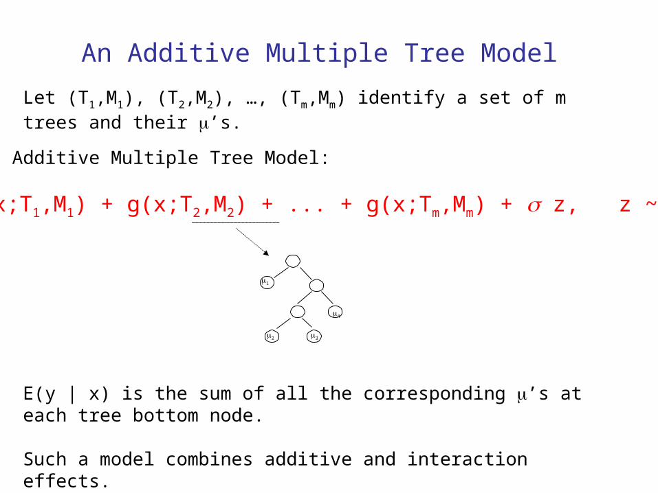
Let (T1,M1), (T2,M2), …, (Tm,Mm) identify a set of m trees and their ’s.

An Additive Multiple Tree Model:

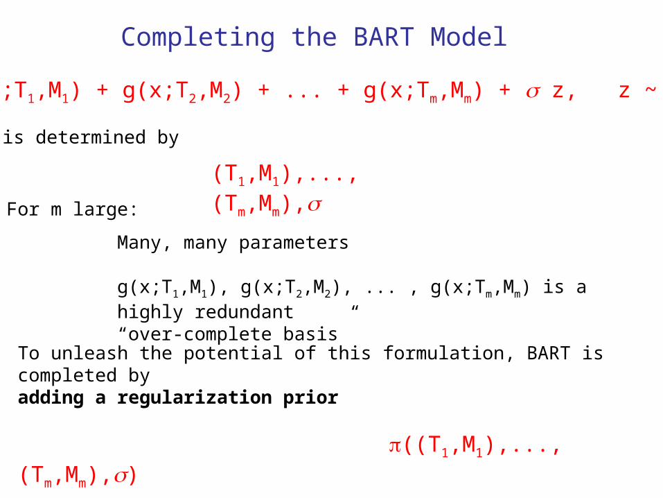
y = g(x;T1,M1) + g(x;T2,M2) + ... + g(x;Tm,Mm) + z, z ~ N(0,1)

An Additive Multiple Tree Model

E(y | x) is the sum of all the corresponding ’s at each tree bottom node.

Such a model combines additive and interaction effects.

1

2 3

4

y = g(x;T1,M1) + g(x;T2,M2) + ... + g(x;Tm,Mm) + z, z ~ N(0,1)

To unleash the potential of this formulation, BART is completed by adding a regularization prior

((T1,M1),...,(Tm,Mm),)

Strongly influential is used to keep each (Ti, Mi) small

Completing the BART Model

(T1,M1),...,(Tm,Mm),

is determined by

Many, many parameters

g(x;T1,M1), g(x;T2,M2), ... , g(x;Tm,Mm) is a highly redundant“over-complete basis”

For m large:

( | y) p(y | ) ( )

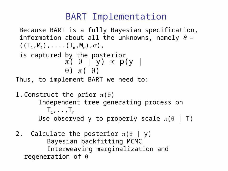
BART Implementation

Because BART is a fully Bayesian specification, information about all the unknowns, namely = ((T1,M1),....(Tm,Mm),),

is captured by the posterior

Thus, to implement BART we need to:

1. Construct the prior () Independent tree generating process on T1,..,Tm

Use observed y to properly scale ( | T)

2. Calculate the posterior ( | y) Bayesian backfitting MCMCInterweaving marginalization and regeneration of

R package BayesTree available on CRAN

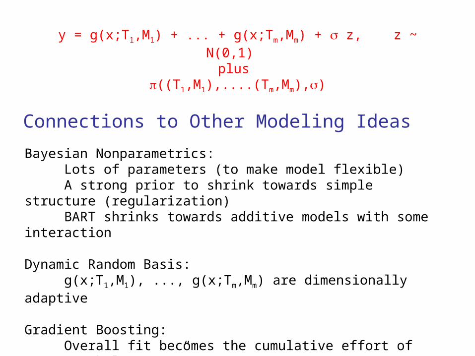
Bayesian Nonparametrics: Lots of parameters (to make model flexible) A strong prior to shrink towards simple structure (regularization) BART shrinks towards additive models with some interaction

Dynamic Random Basis: g(x;T1,M1), ..., g(x;Tm,Mm) are dimensionally adaptive

Gradient Boosting: Overall fit becomes the cumulative effort of many “weak learners”

Connections to Other Modeling Ideas

y = g(x;T1,M1) + ... + g(x;Tm,Mm) + z, z ~ N(0,1) plus

((T1,M1),....(Tm,Mm),)

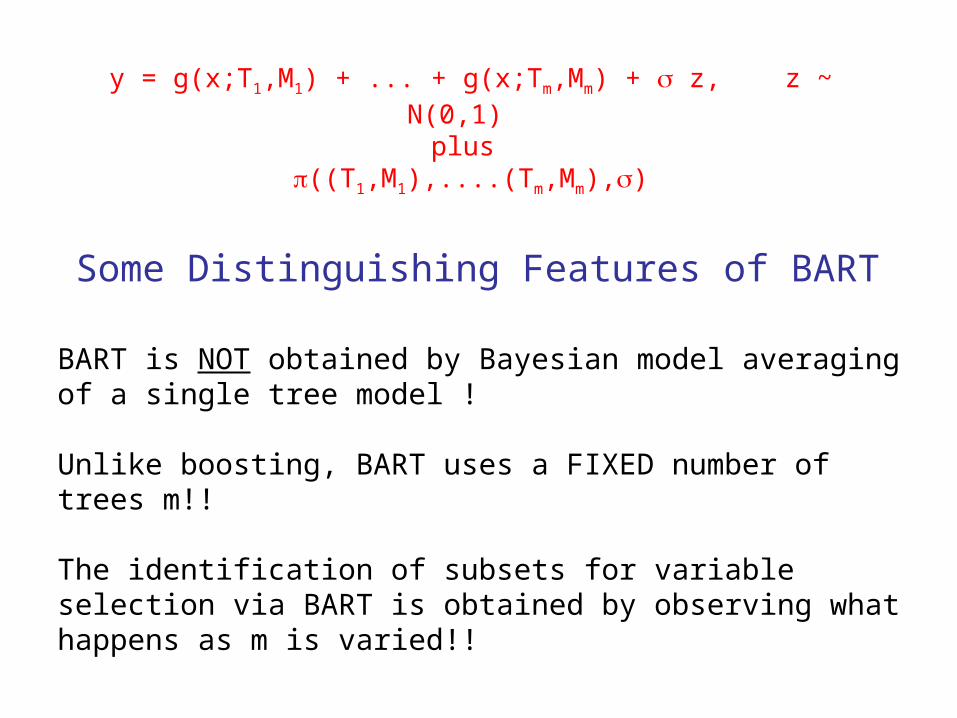
BART is NOT obtained by Bayesian model averaging of a single tree model !

Unlike boosting, BART uses a FIXED number of trees m!!

The identification of subsets for variable selection via BART is obtained by observing what happens as m is varied!!

Some Distinguishing Features of BART

y = g(x;T1,M1) + ... + g(x;Tm,Mm) + z, z ~ N(0,1) plus

((T1,M1),....(Tm,Mm),)

Experimental Comparison on 37 datasets

Neural networks (single layer)Random ForestsBoosting (Friedman's gradient boosting machine)Linear regression with lassoBART (Bayesian Additive Regression Trees)BART/default - *NO* tuning of parameters

Out-sample-performance compared for 6 methods

Data from Kim, Loh, Shih and Chaudhuri (2006) Up to 65 predictors and 2953 observations

Train on 5/6 of data, test on 1/6 Tuning via 5-fold CV within training set 20 Train/Test replications per dataset

Results: Root Mean Squared Errors

Left: RMSE averaged over datasets and replications

Box Plots: RMSE relative to best

BART is a very strong performer!

One of the 37 Datasets is the well-known Boston Housing Data

Each observation corresponds to a geographic district

y = log(median house value)

13 x variables, stuff about the district

eg. crime rate, % poor, riverfront, size, air quality, etc.

n = 507 observations

Each boxplot depicts20 rmse'sout-of-samplefor a versionof a method.

eg.the methodneural netswith a givennumber ofnodes anddecay value.

linear regression

neural nets

Bayesian treed regression

gbm randomforests

BART

Smaller is better.BART wins!

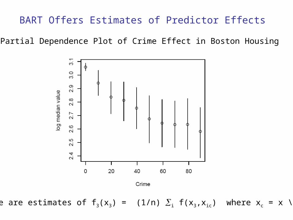
BART Offers Estimates of Predictor Effects

Partial Dependence Plot of Crime Effect in Boston Housing

These are estimates of f3(x3) = (1/n) i f(x3,xic) where xc = x \ x3

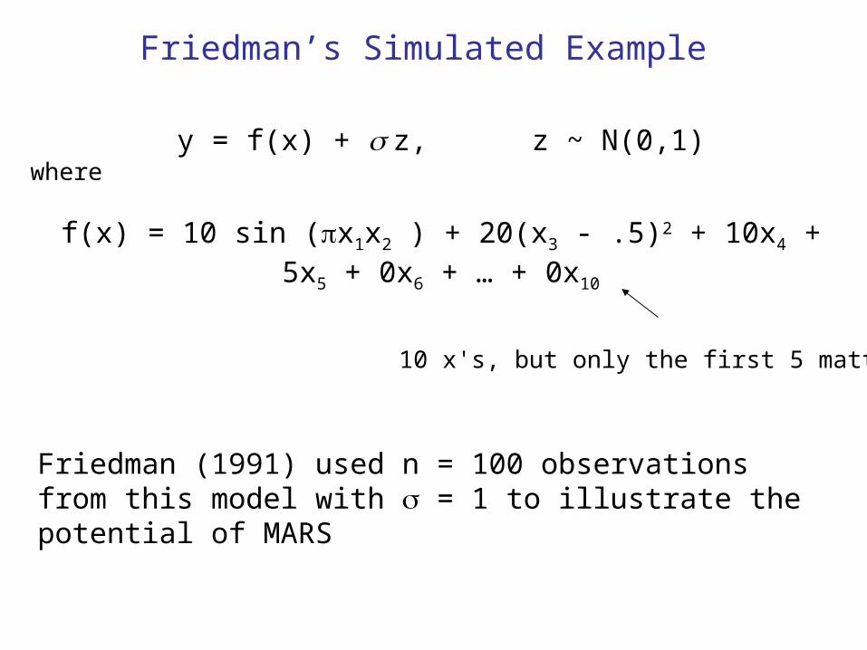
Friedman (1991) used n = 100 observations from this model with = 1 to illustrate the potential of MARS

y = f(x) + z, z ~ N(0,1)where

f(x) = 10 sin (x1x2 ) + 20(x3 - .5)2 + 10x4 + 5x5 + 0x6 + … + 0x10

10 x's, but only the first 5 matter!

Friedman’s Simulated Example

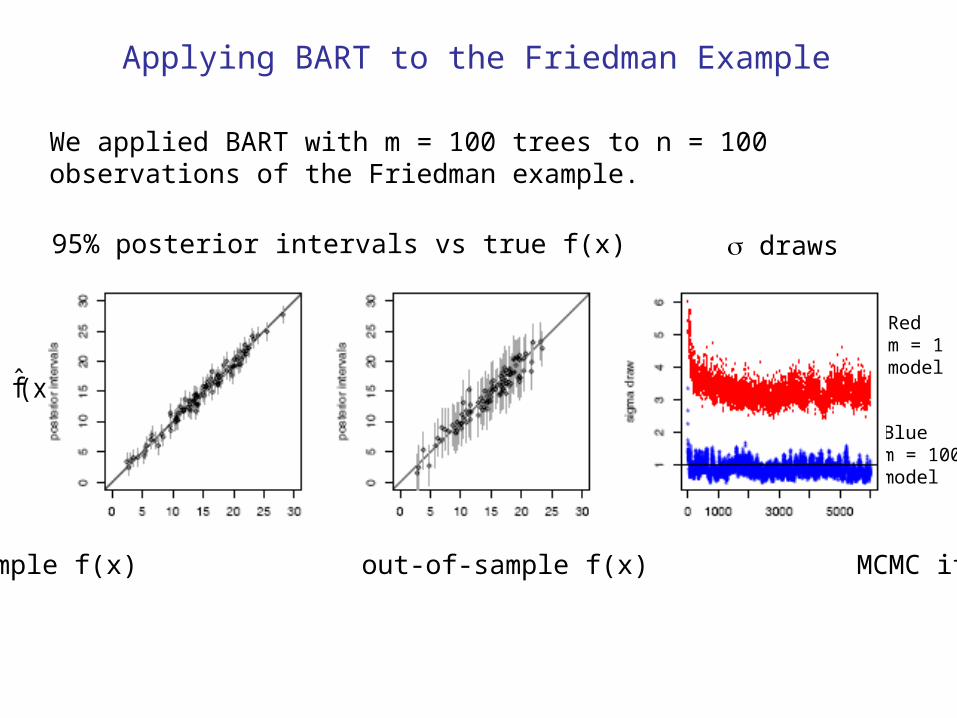
Applying BART to the Friedman Example

Redm = 1model

Bluem = 100model

We applied BART with m = 100 trees to n = 100 observations of the Friedman example.

(x)f

95% posterior intervals vs true f(x) draws

in-sample f(x) out-of-sample f(x) MCMC iteration

Comparison of BART with Other Methods

50 simulations of 100 observations of Friedman example

The cross validation domain used to tune each method

10002

i ii 1

1 ˆRMSE (f(x ) f(x ))1000

Performance measured on 1000 out-of-sample x’s by

BART Wins Again!

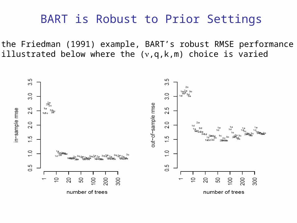
BART is Robust to Prior Settings

On the Friedman (1991) example, BART’s robust RMSE performanceIs illustrated below where the (,q,k,m) choice is varied

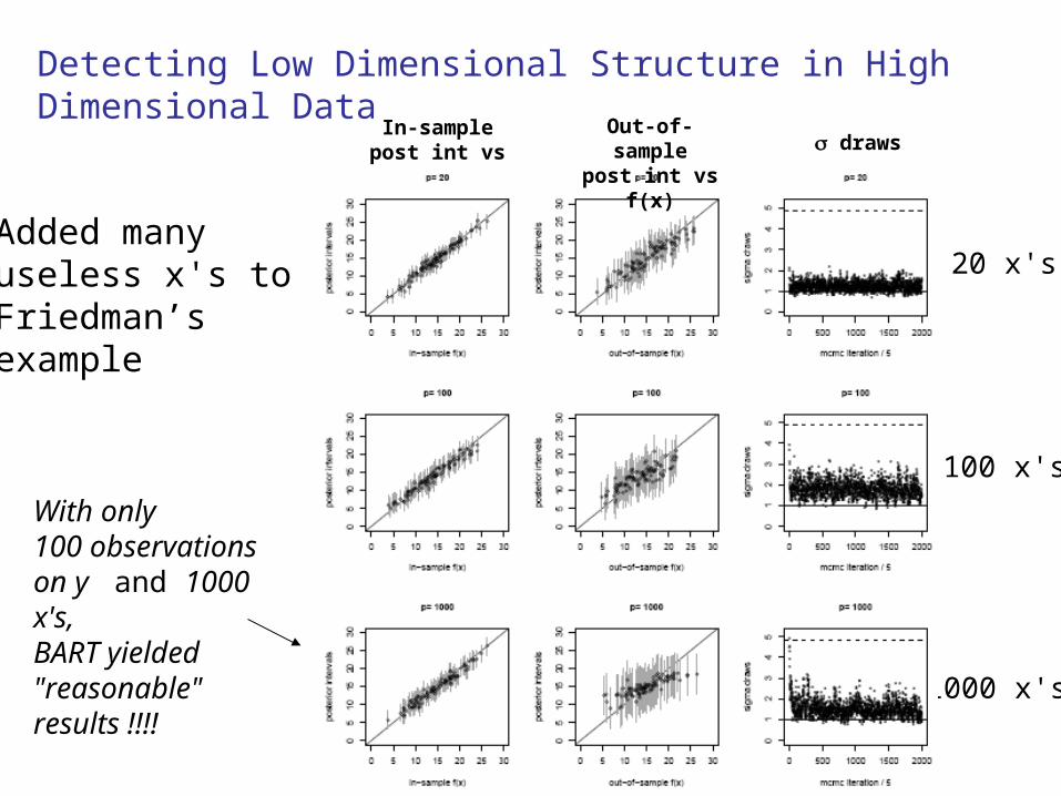
With only100 observationson y and 1000 x's,BART yielded "reasonable"results !!!!

Added manyuseless x's toFriedman’sexample

In-samplepost int vs f(x)

f(x)

20 x's

100 x's

1000 x's

Detecting Low Dimensional Structure in High Dimensional Data

Out-of-samplepost int vs f(x) draws

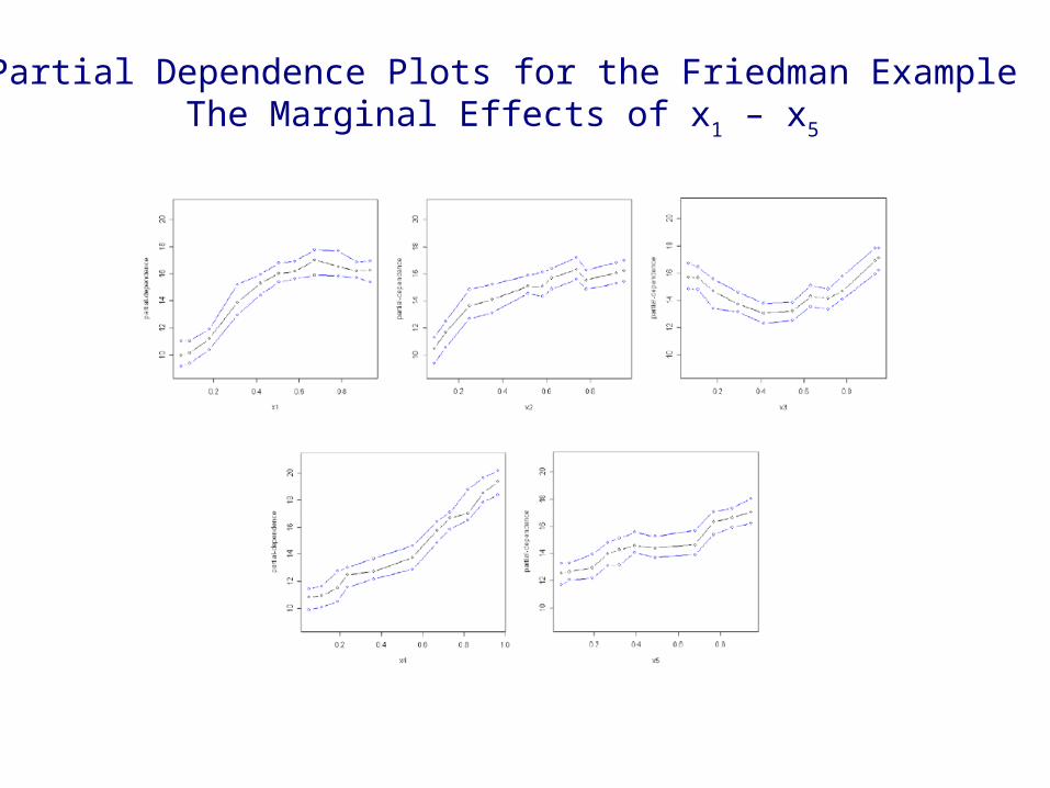
Partial Dependence Plots for the Friedman ExampleThe Marginal Effects of x1 – x5

Partial Dependence Plots for the Friedman ExampleThe Marginal Effects of x6 – x10

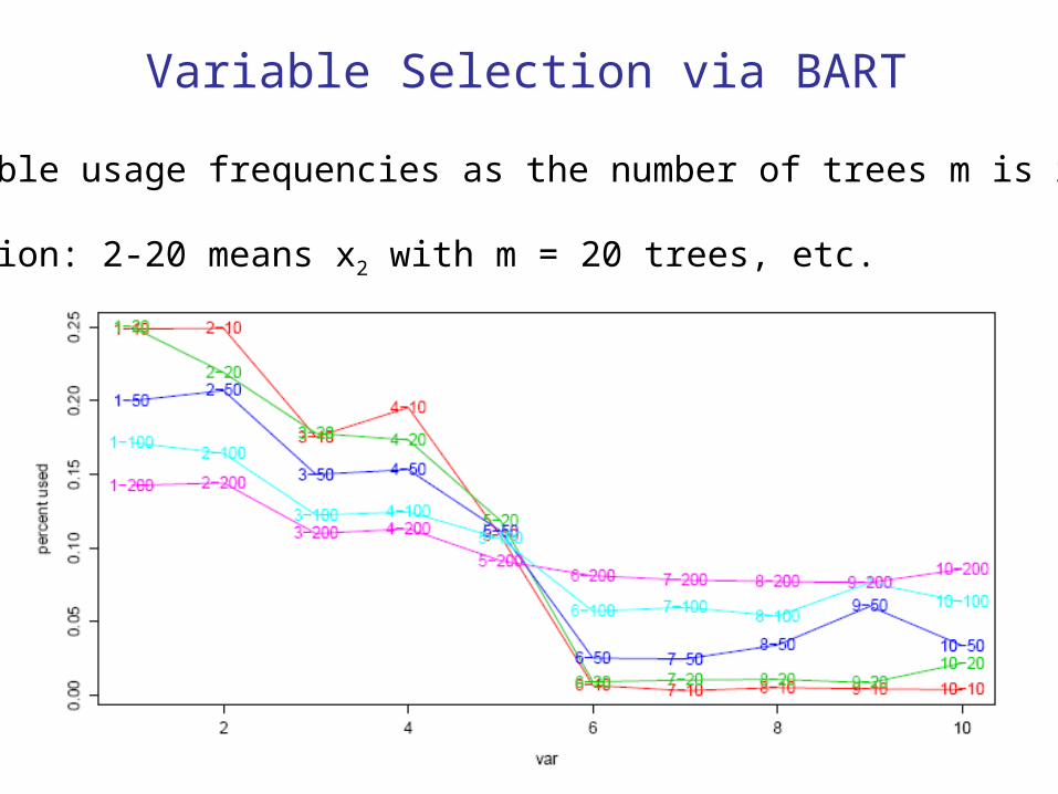
Variable Selection via BART

Variable usage frequencies as the number of trees m is reduced

Notation: 2-20 means x2 with m = 20 trees, etc.

Each observation (n=245) corresponds to an NCAA footballgame.

y = Team A points - Team B points

29 x’s. Each is the difference between the two teams on some measure. eg x10 is average points against defense per game for Team A for team B.

The Football Data

For each draw, for each variable calculate the percentage oftime that variable is used in a tree. Then average over trees.

Variable Selection for the Football Data

Subtle point: Can’t have too many trees. Variables come in without really doing anything.

Marginal Effects of the Variables

Just used variables 2,7,10, and 14.

Here are the four univariate partial-dependence plots.

A Bivariate Partial Dependence PlotThe joint effect of two of the x’s

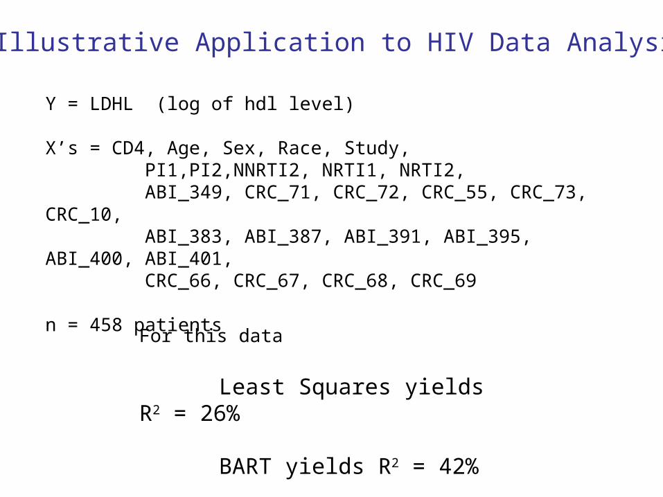
For this data

Least Squares yields R2 = 26%

BART yields R2 = 42%

Y = LDHL (log of hdl level)

X’s = CD4, Age, Sex, Race, Study, PI1,PI2,NNRTI2, NRTI1, NRTI2, ABI_349, CRC_71, CRC_72, CRC_55, CRC_73, CRC_10, ABI_383, ABI_387, ABI_391, ABI_395, ABI_400, ABI_401, CRC_66, CRC_67, CRC_68, CRC_69

n = 458 patients

Illustrative Application to HIV Data Analysis

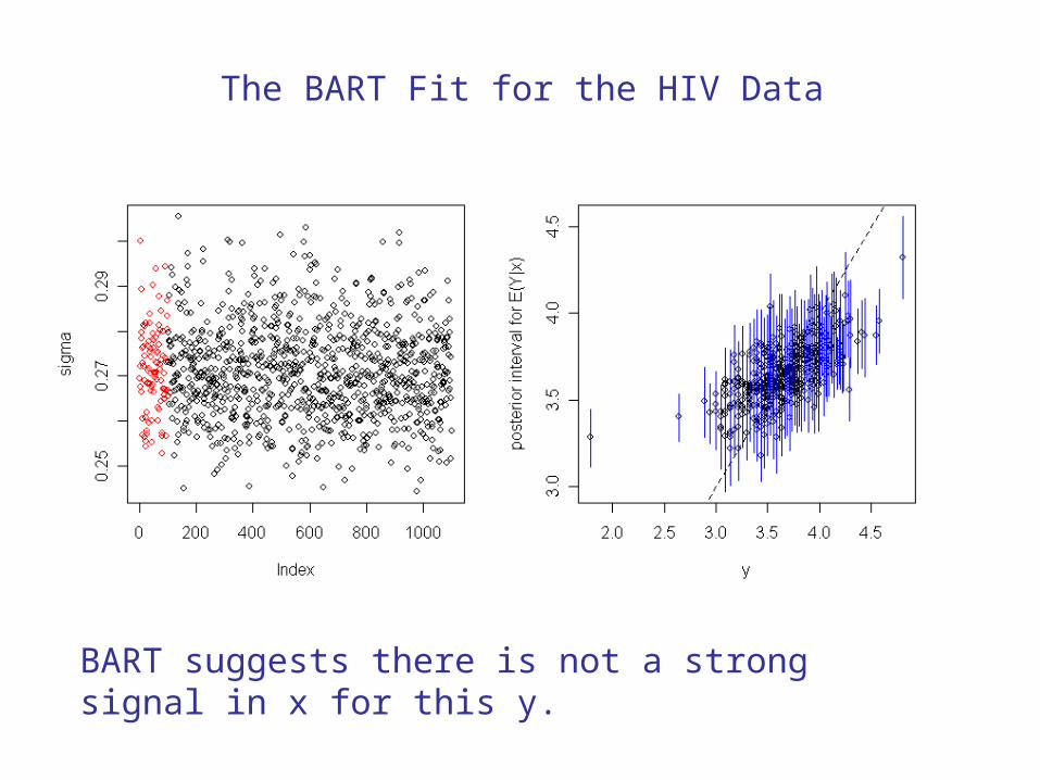
BART suggests there is not a strong signal in x for this y.

The BART Fit for the HIV Data

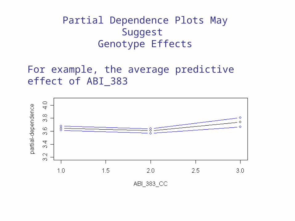
For example, the average predictive effect of ABI_383

Partial Dependence Plots May Suggest Genotype Effects

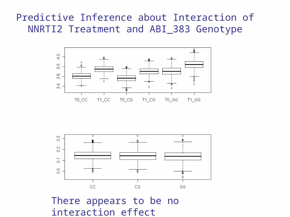
There appears to be no interaction effect

Predictive Inference about Interaction of NNRTI2 Treatment and ABI_383 Genotype

First, introduce prior independence as follows

Thus we only need to choose (T), (), and (| T) = ()

A Sketch of the Prior

((T1,M1),....,(Tm,Mm), ) = [ (Tj,Mj) ] ()

= [ (ij | Tj) (Tj) ] ()

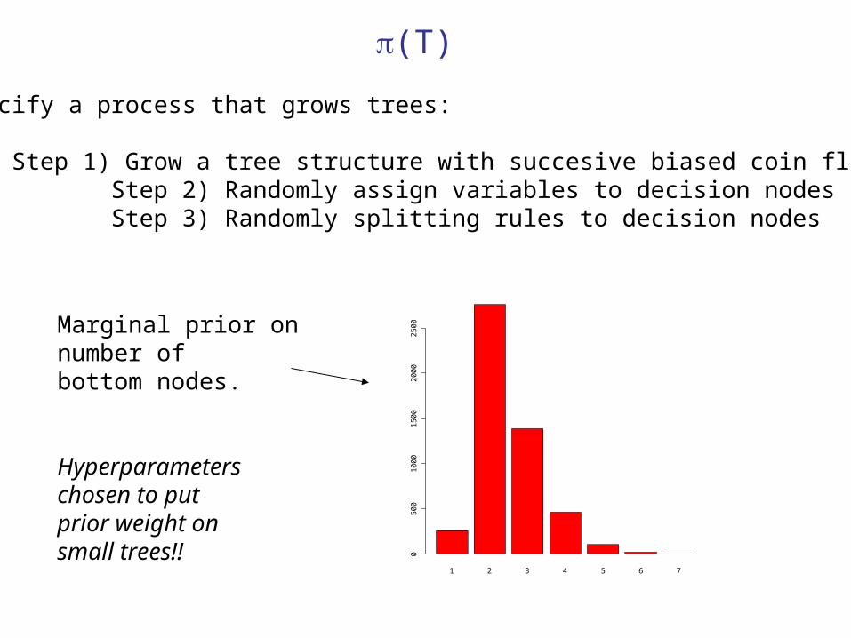
1 2 3 4 5 6 7

05

00

10

00

15

00

20

00

25

00Marginal prior on

number ofbottom nodes.

Hyperparameterschosen to putprior weight onsmall trees!!

We specify a process that grows trees:

Step 1) Grow a tree structure with succesive biased coin flips Step 2) Randomly assign variables to decision nodes Step 3) Randomly splitting rules to decision nodes

(T)

(| T)

To set , we proceed as follows:

First standardize y so that E(y | x) is in [-.5,.5] with high probability.

Note that in our model, E(y | x) is the sum of m independent 's (a priori),so that the prior standard deviation of E(y | x) is m

For each bottom node , let

.5k m .5

k m

Default choice is k = 2.

k is the number of standard deviations of E(y | x) from the mean of 0 to the interval boundary of .5

Note how the prior adapts to m: gets smaller as m gets larger.

)2μσN(0, ~ μ

Thus, we choose so that for a suitable value of k

()

22

~

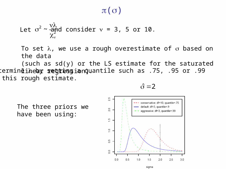
Let

Determine by setting a quantile such as .75, .95 or .99 at this rough estimate.

The three priors we have been using:

ˆ 2

To set , we use a rough overestimate of based on the data (such as sd(y) or the LS estimate for the saturated linear regression).

and consider = 3, 5 or 10.

A Sketch of the MCMC algorithm

The “parameter“ is:

“Simple" Gibbs sampler:

j j

j j i i j i i j

| {T },{M },data

(T ,M ) | {T } ,{M } , ,data

y = g(x;T1,M1) + g(x;T2,M2) + ... + g(x;Tm,Mm) + z

(1)

(2)

(1) Subtract all the g's from y to update (2) Subtract all but the jth g from y to update (Tj,Mj)

(Bayesian backfitting)

= ((T1,M1),....(Tm,Mm),)

j j i i j i i j(T ,M ) | {T } ,{M } , ,data

Using the decomposition

and the fact that p(T | data) is available under our prior, we sample

p(T,M | data) = p(T | data) p(M | T, data)

by first drawing T from p(T | data), and then drawing M from p(M | T, data).

Drawing M from p(M | T,data) is routine

Just simulate ’s from the posterior under a conjugate prior

To draw T from p(T | data), we use a Metropolis-Hastings algorithm.

Given the current T, we propose a modification andthen either move to the proposal or repeat the old tree.

In particular we use proposals that change the size of the tree:

=>

?

=>

?propose a more complex tree

propose a simpler tree

More complicated models will be accepted if the data's insistenceovercomes the reluctance of the prior.

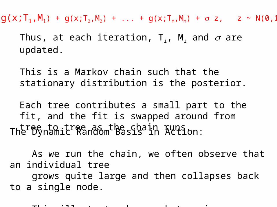
y = g(x;T1,M1) + g(x;T2,M2) + ... + g(x;Tm,Mm) + z, z ~ N(0,1)

Thus, at each iteration, Ti, Mi and are updated.

This is a Markov chain such that the stationary distribution is the posterior.

Each tree contributes a small part to the fit, and the fit is swapped around from tree to tree as the chain runs.

The Dynamic Random Basis in Action: As we run the chain, we often observe that an individual tree grows quite large and then collapses back to a single node.

This illustrates how each tree is dimensionally adaptive.

At iteration i we have a draw from the posterior of the function

To get in-sample fits we average the

Posterior uncertainty is captured by variation of the

Using the MCMC Output to Draw Inference

)M,T,g( )M,T,g( )M,T,g( )(f mimi2i2i1i1ii ˆ

)(f obtain to draws )(f ii ˆ

(x)fi

f(x). estimates (x)f Thus, i

BART (and probably other nonparametric methods) can give us a sense of

• E(y |x)• the distribution of y around E(y|x)• the individual effects of the xj’s

• a subset of x1,...,xp related to y

This information would seem to be very valuable for model building. The next step is how?

Where do we go from here?

To be continued…