Practical Exam: Airy Disks - usna.edu

Practical Exam: Airy Disks MIDN Charles Stabler

20 OCT 2016

Professor Avramov-Zamurovic

ES485A

Introduction

For this practical exam, we were required to research Airy Disks, predict the locations of the disks based on three different aperture diameters, and photograph the disks to compare predicted locations with experimental locations. Airy Disks are the formation of light patterns that occur when light passes through a small aperture. Study of these patterns has led to the formation of mathematical models that predict the distance of maxima and minima of the disks from the center of light; in our case, light from a red laser beam. A quick search of the Internet revealed the relatively simple formula for this prediction. Perhaps more interesting are the patterns developed from two side-by-side apertures or three apertures in a triangle formation, which we were able to observe and photograph; examples of which are included in this report. Ultimately, the mathematical model did not align with the experimental results, and further experimentation would be required to discover the reason.

Mathematical Prediction

The mathematical model for the locations of the Airy Disks is relatively simple. Using the

small angle approximation for sine, the wavelength of the laser light 𝜆, the distance of the aperture from the target where the beam was photographed 𝐷, the diameter of the apertures 𝑑,

and experimental constants for each minima and maxima 𝑚; we can predict the distance of the minima or maxima 𝑦 from the center of the beam:

𝑦 = 𝐷𝑚𝜆

𝑑 . (1)

For each of the three apertures, three minima and maxima were predicted. The source used was a red laser light with wavelength 632.8 nm, whose beam was immediately expanded and passed through the aperture. A camera was set up 4.5 m downrange, with 0.9 power intensity filter and a red light filter. The results of these predictions are in the following tables.

Aperture d = 0.7366 mm

Number of Minima or Maxima

Minima Distance

(mm)

Maxima Distance

(mm)

1 4.7164 6.3207

2 8.6325 10.3567

3 12.5177 14.2651

Table 1 Predictions for distance of minima and maxima from beam center for the small aperture



Minima Distance

(mm)

Maxima Distance

(mm)

1 3.3360 4.4707

2 6.1059 7.3254

3 8.8540 10.0899

Table 2 Predictions for distances of minima and maxima from the beam center for the medium aperture



Minima Distance

(mm)

Maxima Distance

(mm)

1 1.7535 2.3500

2 3.2095 3.8506

3 4.6540 5.3037

Table 3 Predictions for the distances of minima and maxima from the beam center for the large aperture

A recognizable trend occurs with an increase in aperture size. As the aperture diameter increases, the distances of the disks from the center of the beam are reduced. Further research unveiled that this trend is due to the wave properties of light; that a smaller aperture closer in size to the wavelength of the light causes more spreading than an aperture that relatively larger than the wavelength of the light.

Setup

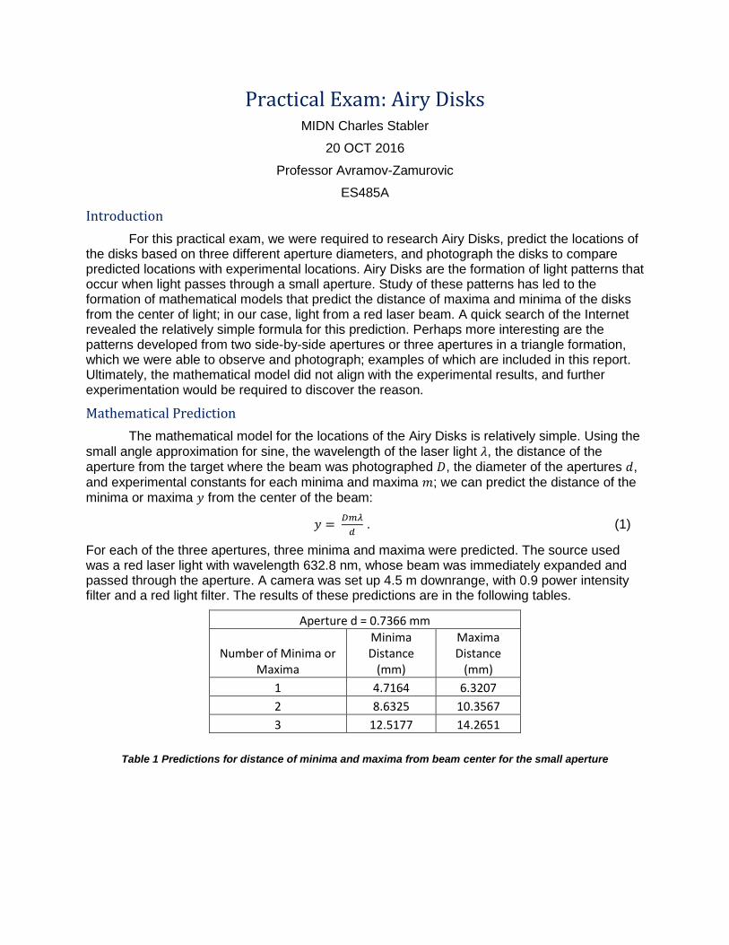
A portion of this practical exam was setting up the experiment. To obtain the most accurate results, the laser was directed onto the camera sensor. Knowing the size of sensor and each pixel, an accurate measure could be taken of the minima and maxima. The images were captured by moving the camera perpendicular to the beam propagation path for each maxima of the Airy Disk. For the imaging software, the same settings could not be used for each image of an aperture because the second and third disks were not visible. This did not affect the intensity measurement on the sensor, however. In addition to directing the beam onto the sensor, we photographed the beam and subsequent Airy Disks on a white target with a 17 mm lens, and again with an iPhone camera to best represent what the eye sees.

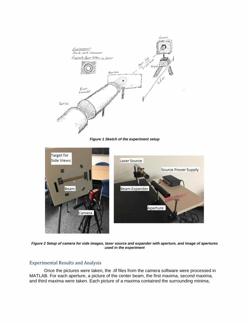
Figure 1 Sketch of the experiment setup

Figure 2 Setup of camera for side images, laser source and expander with aperture, and image of apertures used in the experiment

Experimental Results and Analysis

Once the pictures were taken, the .tif files from the camera software were processed in MATLAB. For each aperture, a picture of the center beam, the first maxima, second maxima, and third maxima were taken. Each picture of a maxima contained the surrounding minima,

which was how the measurements were standardized. To calculate the minima and maxima, the ‘findpeaks’ function was used. The results are shown in Tables 4-6.



Predicted Minima Distance

(mm)

Experimental Minima Distance

(mm)

Predicted Maxima

Distance (mm)

Experimental Maxima

Distance (mm)

1 4.7164 3.5960 6.3207 4.6838

2 8.6325 6.4524 10.3567 7.8214

3 12.5177 9.3532 14.2651 10.6778

Table 4 Results of experiment with mathematical predictions for small aperture




(mm)


(mm)

Predicted Maxima

Distance (mm)

Experimental Maxima

Distance (mm)

1 3.3360 2.7338 4.4707 4.0140

2 6.1059 5.4940 7.3254 6.5596

3 8.8540 8.1580 10.0899 9.3124

Table 5 Results of experiment with mathematical predictions for medium aperture




(mm)


(mm)

Predicted Maxima

Distance (mm)

Experimental Maxima

Distance (mm)

1 1.7535 2.9230 2.3500 3.8998

2 3.2095 5.8830 3.8506 6.9782

3 4.6540 7.8736 5.3037 10.1824

Table 6 Results of experiment with mathematical predictions for large aperture

Overall, an interesting trend is observed from the results. For the small aperture, the prediction overshoots the values for the experimental results. The medium aperture has a smaller deviation, though the prediction again overshoots the experimental results. For the large aperture, the prediction undershoots the experimental data by nearly half for each value. It would be interesting to see these results replicated at a farther and shorter distance between the aperture and the camera sensor. Figure 2 shows an example of how the locations of the distances of the rings from the center were calculated.

Figure 3 Using ‘findpeaks’ to measure distances of maxima and minima from the center of the beam for the medium aperture, d = 1.0414 mm. The locations of each point were recorded, and differences between

the minima and maxima were taken to find total distance from the center. Figure 2.A is the center maxima; 2.B is m=1 minima, m=1 maxima, and m=2 minima; 2.C is m=2 minima, m=2 maxima, and m=3 minima; 2.D is

m=3 minima, m=3 maxima, and m=4 minima. Note that the distances on the axis do not correlate with the actual distance from the center maxima, though the labeled distances on the lines do correlate. Also, the y-

axis range changes for each portion to best show the quality of each maxima.

Visually, the Airy Disk pattern are pleasing to the eye. For a larger aperture, the disks are noticeably finer and closer together; and for the smaller aperture, the rings are wider and the edges are less sharp and almost appear out of focus. Pictures of the rings as the eye would see them are in Figure 3.

Figure 4 Pictures taken of Airy Disks, left to right is 0.7366 mm, 1.0414 mm, and 1.9812 mm in aperture diameter.

As the camera views the images from the side with a 17 mm lens, the images are less exciting though the intensity gradient is more clearly defined. The intensity of the outer rings is much less than that of the center beam or m = 1 and m = 2 ring.

Figure 5 Camera views highlighting intensity, from 0.7366 mm, 1.0414 mm, and 1.9812 mm left to right. The values of the axes are in pixels, which serve only to document the relative size of each image.

Figure 6 Cross section of relative intensity of d = 0.7366 mm aperture. Red lines indicate a maxima and black lines indicate a minima. The center lobe of the beam was cut off to better view the maxima and minima.

Figure 7 Cross section of relative intensity of d = 1.0414 mm aperture. Red lines indicate a maxima and black lines indicate a minima. The center lobe of the beam was cut off to better view the maxima and minima.

Figure 8 Cross section of the relative intensity of the d = 1.9812 mm aperture. Red lines indicate a maxima and black lines indicate a minima. The center lobe of the beam was cut off to better view the maxima and

minima.

With the camera set up such that the beam was directly impacting the sensor, the

relative intensity of the light was measured. The camera used has 214 values to measure light, allowing precise measurement of light intensity from the beam. Using experimental coefficients for each relative intensity of a given m-value, the intensity of the disk can be compared to the intensity of the central beam. The comparison between the predicted relative intensities and measured relative intensities are shown in Figure 5.

Figure 9 Comparison of relative intensities, predicted and measured. From left to right, the small to large aperture. Predicted relative intensities are in red and actual relative intensities are in blue.

To note from the graphs of the relative intensities, the measured intensities are larger than the predicted intensities. However, all follow an exponential decrease pattern as the m-value increases. Each measured relative intensity was found by dividing the intensities of the maxima by the maximum intensity of the central portion of the beam.

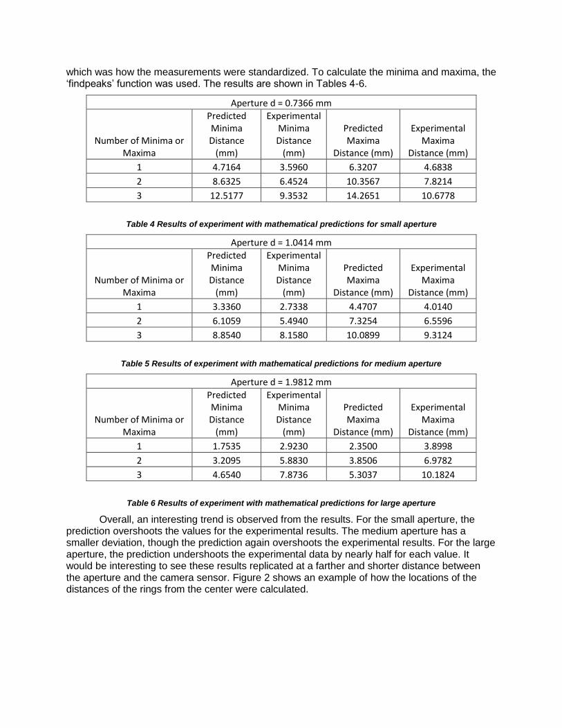
For further experimentation, we viewed the patterns of the beam passed through two apertures side-by-side and a triangular formation of apertures. No mathematical model exists for these patterns due to their complication. However, they are interesting to view, shown in Figures 6 and 7.

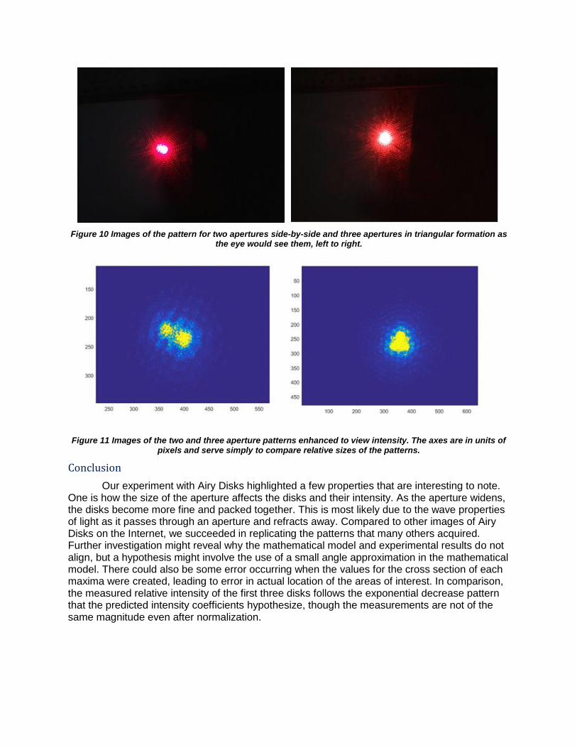
Figure 10 Images of the pattern for two apertures side-by-side and three apertures in triangular formation as the eye would see them, left to right.

Figure 11 Images of the two and three aperture patterns enhanced to view intensity. The axes are in units of pixels and serve simply to compare relative sizes of the patterns.

Conclusion

Our experiment with Airy Disks highlighted a few properties that are interesting to note. One is how the size of the aperture affects the disks and their intensity. As the aperture widens, the disks become more fine and packed together. This is most likely due to the wave properties of light as it passes through an aperture and refracts away. Compared to other images of Airy Disks on the Internet, we succeeded in replicating the patterns that many others acquired. Further investigation might reveal why the mathematical model and experimental results do not align, but a hypothesis might involve the use of a small angle approximation in the mathematical model. There could also be some error occurring when the values for the cross section of each maxima were created, leading to error in actual location of the areas of interest. In comparison, the measured relative intensity of the first three disks follows the exponential decrease pattern that the predicted intensity coefficients hypothesize, though the measurements are not of the same magnitude even after normalization.

Appendix

MIDN Charles Stabler

% This code predicts minima and maxima of airy disks from center of beam,

% imports .tif images of beams, analyzes those images by measurement and

% beam intensity, and graphically displays results.

Airy Disk maxima and minima prediction

lambda = 632.8e-6; % wavelength of laser light, nm

d1 = 0.7366e-3; % single-hole aperture sizes, mm

d2 = 1.0414e-3;

d3 = 1.9812e-3;

D = 4.5; % distance from aperture to target, where Airy disks measured

minim = [1.220 2.233 3.238]; % vector of minima m values

maxim = [1.635 2.679 3.69]; % vactor of maxima m values

relint = [0.0175 0.0042 0.00078]; % vector of predicted maxima relative intensities to beam

% rows are predicted maxima/minima values for an aperture, apertures

% increase down columns

ymax = [maxim.*lambda*D/d1; maxim.*lambda*D/d2; maxim.*lambda*D/d3];

ymin = [minim.*lambda*D/d1; minim.*lambda*D/d2; minim.*lambda*D/d3];

Reading in images for analysis

InfoImage = imfinfo('1holeLarge0.tif'); % getting image info

Image = InfoImage(1).Width; % variable for width of image

nImage = InfoImage(1).Height; % variable for height of image

im0 = imread('1holeLarge0.tif');



im3 = imread('1holeLarge3.tif');% reading individual pixel values and assigning variable for

array

% im0 = imread('1holeMedium0.tif');




% im0 = imread('1holeSmall0.tif');




Pretty side view images

% im = imread('1holeLargeSideView.tif');

% im = imread('1holeMediumSideView.tif');

im = imread('1holeSmallSideView.tif');



z = min(min(im)); % minimum pixel value

zz = max(max(im)); % maximum pixel value

aa = ceil(((im-z)./255));

figure,clf;

image(aa)

pixsz = 7.4e-6;

lngth = -319*pixsz:pixsz:320*pixsz;

avgcol = AvgCol(im0,Image);

avgcolsm = smooth(avgcol);

[pks,locs] = findpeaks(avgcolsm,lngth,'MinPeakDistance',4e-3);

centloc = locs - -319*pixsz; % -0.002227 for small % -0.001831 for medium % -319*pixsz for large

% beam center

halfbeam0 = zeros(2,320);

halfbeam0(1,:) = fliplr(avgcolsm(1:320));

halfbeam0(2,:) = pixsz:pixsz:320*pixsz;

figure(1),clf;

hold on

plot(lngth,avgcolsm)

plot(locs,pks,'r*')

xlabel('Distance (mm)')

ylabel('Intensity')

grid on

lngth = pixsz:pixsz:Image*pixsz; % converting pixels to length vector

avgcol = AvgCol(im1,Image); % average intensity vector for each column


[pks,locs] = findpeaks(avgcolsm,lngth,'MinPeakDistance',1e-3); % finding peaks for maxima

[mins,locmin] = findpeaks(-1*avgcolsm,lngth,'MinPeakDistance',2e-3); % finding minima

dist12 = diff(locmin); % distance between minima

min1 = locmin(1); % isolating location of first minima in image

min21 = locmin(2); % isolating location of second minima in image

max1 = locs(2); % isolating maxima in image

minmax11 = max1 - min1; % difference between m = 1 minima and maxima

minmax12 = min21 - max1; % difference between m = 1 maxima and m = 2 minima

g1 = floor((locmin(2)-locmin(1))/pixsz); % size of needed array for continuous cross section

halfbeam1 = zeros(2,g1+1); % creating matrix for both lengths and intensities for continuous

cross section

halfbeam1(1,:) = avgcolsm(locmin(1)/pixsz:floor(locmin(2)/pixsz)); % populating continous cross

section matrix

halfbeam1(2,:) = halfbeam0(2,end) + lngth(locmin(1)/pixsz:floor(locmin(2)/pixsz));

% For m = 1,2 minima; m = 2 maxima

figure(2),clf;

hold on


plot(locs(2),pks(2),'r*')

plot(locmin,-mins,'y*')


ylabel('Intensity')

grid on




[mins,locmin] = findpeaks(-1*avgcolsm,lngth,'MinPeakDistance',2.5e-3);

dist23 = diff(locmin);

max2 = locs(2);

min22 = locmin(1);

min31 = locmin(2);

minmax22 = min22 - max2;

minmax23 = min31-max2;

g2 = floor((locmin(2)-locmin(1))/pixsz);

halfbeam2 = zeros(2,g2+1);

halfbeam2(1,:) = avgcolsm(floor(locmin(1)/pixsz):floor(locmin(2)/pixsz));

halfbeam2(2,:) = halfbeam1(2,end) + lngth(floor(locmin(1)/pixsz):floor(locmin(2)/pixsz));

% For m = 2,3 minima, m = 2 maxima

figure(3),clf;

hold on





ylabel('Intensity')

grid on




[mins,locmin] = findpeaks(-1*avgcolsm,lngth,'MinPeakDistance',2.5e-3);

dist34 = diff(locmin);

min32 = locmin(1);

min4 = locmin(2);

max3 = locs(2);

minmax3 = min32 - max3;

g3 = floor((locmin(2)-locmin(1))/pixsz);

halfbeam3 = zeros(2,g3+1);

halfbeam3(1,:) = avgcolsm(floor(locmin(1)/pixsz):floor(locmin(2)/pixsz));

halfbeam3(2,:) = halfbeam2(2,end) + lngth(floor(locmin(1)/pixsz):floor(locmin(2)/pixsz));

% For m = 3,4 minima; m = 3 maxima

figure(4),clf;

hold on





ylabel('Intensity')

grid on

% This piece of code calculates the distances of the locations of the m = #

% maxima and minima, using the minima as reference points for each

% successive image.

minmaxT = [centloc+min1; centloc+max1; centloc+min21; centloc+min21-min22+max2; centloc+min21-

min22+min31; centloc+min21-min22+min31-min32+max3];

maxintens = max(max(im0));

predictintens = double(maxintens).*[0.0175 0.0042 0.00078]; % finding maximum intensity for the

beam, then multiplying by coefficients for m = 1,2,3

actintens = [max(max(im1(:,200:600))) max(max(im2(:,200:600))) max(max(im3(:,200:600)))];

compintens = cat(1,predictintens,actintens);

m = [1 2 3];

figure(5),clf;

grid MINOR

plot(m,predictintens,'r*',m,actintens,'b*')

ylabel('Relative Intensity')

xlabel('M value')

axis([0 3.5 0 max(actintens)+50])

% Making the concatenated vectors of beam center to third disk

halfbeam = zeros(2,321+g1+g2+g3+2);

halfbeam(1,:) = cat(2,halfbeam0(1,:),halfbeam1(1,:),halfbeam2(1,:),halfbeam3(1,:));

halfbeam(2,:) = cat(2,halfbeam0(2,:),halfbeam1(2,:),halfbeam2(2,:),halfbeam3(2,:));

figure(6),clf;

plot(halfbeam(2,:),halfbeam(1,:))



grid MINOR

imS = imread('1holeSmallSideView.tif');

imM = imread('1holeMediumSideView.tif');

imL = imread('1holeLargeSideView.tif');

figure(7),clf;

plot(imS(203,:))


xlabel('Pixels')

axis([0 640 0 1200])

figure(8),clf;

plot(imM(250,:))


xlabel('Pixels')

axis([0 640 0 1200])

figure(9),clf;

plot(imL(280,:))


xlabel('Pixels')

axis([0 640 0 1200])

AvgCol Function This function calculates the average value of a column of intensities from an image of a laser beam in order to plot the averages to find max intensities.

function [avgcol] = AvgCol(im,numpix)

avgcol = zeros(numpix,1);

for ii = 1:numpix

avgcol(ii) = mean(im(:,ii));

end

end

Published with MATLAB® R2016a

http://www.mathworks.com/products/matlab

Practical Exam: Airy Disks - usna.edu

Documents