Practical Aspects of Free-Energy Calculations: A Review

Practical Aspects of Free-Energy Calculations: A ReviewNiels Hansen†,‡,* and Wilfred F. van Gunsteren‡

†Institute of Thermodynamics and Thermal Process Engineering, University of Stuttgart, D-70569 Stuttgart, Germany‡Laboratory of Physical Chemistry, Swiss Federal Institute of Technology, ETH, CH-8093 Zurich, Switzerland

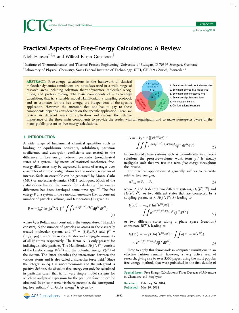
ABSTRACT: Free-energy calculations in the framework of classicalmolecular dynamics simulations are nowadays used in a wide range ofresearch areas including solvation thermodynamics, molecular recog-nition, and protein folding. The basic components of a free-energycalculation, that is, a suitable model Hamiltonian, a sampling protocol,and an estimator for the free energy, are independent of the specificapplication. However, the attention that one has to pay to thesecomponents depends considerably on the specific application. Here, wereview six different areas of application and discuss the relativeimportance of the three main components to provide the reader with an organigram and to make nonexperts aware of themany pitfalls present in free energy calculations.

1. INTRODUCTION

A wide range of fundamental chemical quantities such asbinding or equilibrium constants, solubilities, partitioncoefficients, and adsorption coefficients are related to thedifference in free energy between particular (non)physicalstates of a system.1 By means of statistical mechanics, free-energy differences may be expressed in terms of averages overensembles of atomic configurations for the molecular system ofinterest. Such an ensemble can be generated by Monte Carlo(MC) or molecular-dynamics (MD) techniques. Much of thestatistical-mechanical framework for calculating free energydifferences has been developed some time ago.2−6 The freeenergy F of a system in the canonical ensemble (i.e., at constantnumber of particles, volume, and temperature) is given as

∫ ∫= − ! − − F k T h N p rln{[ ] e d d }N H p r k T N NB

3 1 ( , )/N NB

(1)

where kB is Boltzmann’s constant, T the temperature, h Planck’sconstant, N the number of particles or atoms in the classicallytreated molecular system, and r N = (r1,r2,...rN) and p N =(p 1,p2,...pN) the Cartesian coordinates and conjugate momentaof all N atoms, respectively. The factor N! is only present forindistinguishable particles. The Hamiltonian H(p N, r N) consistsof the kinetic energy K(p N) and the potential energy V(r N) ofthe system. The latter describes the interactions between thevarious atoms and is also called a molecular force field.7 Sincethe integral in eq 1 is 6N-dimensional and the integrand ispositive definite, the absolute free energy can only be calculatedin particular cases, that is, for very simple model systems forwhich an analytical expression for the partition function can beobtained. In an isothermal−isobaric ensemble, the correspond-ing free enthalpy8 or Gibbs energy9 is given by

∫ ∫ ∫= − !

−

− +

G k T Vh N

p r V

ln{[ ]

e d d d }

N

H p r pV k T N N

B3 1

[ ( , ) ]/N NB

(2)

In condensed phase systems such as biomolecules in aqueoussolutions the pressure−volume work term pV is usuallynegligible such that we use the term f ree energy throughoutthis review.For practical applications, it generally suffices to calculate

relative free energies,

Δ = −F F FBA B A (3)

where A and B denote two different systems, HA(p N, r N) andHB(p

N, r N), or two different states that are connected by acoupling parameter λ, H(p N, r N; λ) leading to

∫ ∫λ′ = − !

λ

λ

−

− ′

F k T h N

p r

( ) ln{[ ]

e d d }

N

H p r k T N N

B3 1

( , ; )/N NB

(4)

or two different states along a phase space (reaction)coordinate R(r N), leading to

∫ ∫ δ′ = − ! ′ −

×

−

−

F R k T h N R R r

p r

( ) ln{[ ] ( ( ))

e d d }

RN N

H p r k T N N

B3 1

( , )/N NB (5)

How to apply this framework in computer simulations in aneffective fashion remains, however, a very active area ofresearch, giving rise to over 3500 papers using the most popularfree energy methods that were published in the first decade of

Special Issue: Free Energy Calculations: Three Decades of Adventurein Chemistry and Biophysics

Received: February 24, 2014Published: May 20, 2014

Perspective

pubs.acs.org/JCTC

© 2014 American Chemical Society 2632 dx.doi.org/10.1021/ct500161f | J. Chem. Theory Comput. 2014, 10, 2632−2647

pubs.acs.org/JCTC

this century with the publication rate increasing ∼17% peryear.10 This rapid development comes at the price that it isincreasingly difficult for researchers to find their way throughthe maze of available computational techniques. For reviews onthe methodology to calculate free energy via molecularsimulation, we refer to the literature.11−20 Reviews that aremore application oriented can be found in refs 21−23. Nosingle method for free-energy calculation can be considered asclearly superior to the others, and the proper choice dependsvery much on the system under consideration. Christ et al.18

identified three main challenges that have to be met in freeenergy estimation from molecular simulation, which are (i) thechoice of a suitable model Hamiltonian, (ii) the choice of asampling protocol that allows generating a representativeensemble of configurations, and (iii) the choice of an estimatorfor the free energy difference. The aim of the latter review wasto enable the reader to classify the vast array of methods byidentifying which choices have to be made for these three basiccomponents. Here, we attempt to enable the reader to be awareof the various peculiarities and pitfalls that are characteristic forthe various (bio)molecular systems for which free-energycalculations are performed. We do this by discussingequilibrium free-energy computation from the systems pointof view.In classical molecular simulation three categories of free-

energy differences can be distinguished, which are conforma-tional, alchemical, and thermodynamic free energy differences.Conformational free-energy differences refer to differencesbetween two distinct conformational states (e.g., a left and aright-handed helix) of the same system. Alchemical free-energydifferences refer to differences between two states differing intheir Hamiltonian. Thermodynamic free-energy differencesrefer to differences between two thermodynamic state points(e.g., two different temperatures). In this review, we focus onthe first two types of calculations, their differences can be statedas follows. The free-energy difference between two conforma-tional states is a logarithmic measure of the relative partitionfunctions corresponding to a common Hamiltonian butintegrated over different regions of configurational space ofthe system. The free-energy difference between two alchemicalstates is a logarithmic measure of the relative partition functionscorresponding to the entire space in terms of the degrees offreedom of the system, but performed considering two differentHamiltonians (that are both functions of the same number ofdegrees of freedom).Due to the explosion in the number of publications since the

early 1990s no review of the state of the art can hope to becomprehensive. However, there is broad consensus about thenecessity of further methodological developments and thedefinition of best practices in all areas of applications in(bio)molecular modeling, of which the main ones are (i)solvation of small neutral molecules, (ii) solvation of larger(drug-like) heteromolecules, (iii) solvation of (single)monatomic ions, (iv) solvation of polyatomic ions, (v)noncovalent binding, and (vi) conformational changes. In thefollowing these application areas are reviewed separately withan eye to identify current obstacles and challenges.

2. SOLVATION OF SMALL NEUTRAL MOLECULESThe free energy of solvation corresponds to the free energy oftransferring a compound from a well-defined state (gas) toanother (solution), allowing a direct comparison with experi-ment. The calculation of the free energy of solvation usually

involves an alchemical transformation and was one of the firstpractical applications of the free energy perturbation andintegration methodology.21,22,24 Today, solvation free energiesremain of primary importance for developing and testing forcefields, for testing new methodology, for gaining fundamentalinsights into the solvation process, and for specific applicationssuch as predicting how molecular compounds will partitionbetween different environments.Condensed-phase or biomolecular force fields (e.g.,

CHARMM,25−29 AMBER,30−33 OPLS,34−38 and GRO-MOS39−49) mainly aim at the description of (bio)moleculesin solution. They focus on the description of torsional-angleproperties, nonbonded interactions, and solvation effects.However, the parameter sets used to describe most compoundshave historically been based primarily on structural propertiesand fitting to results from quantum-mechanical calcula-tions.50,51 This is despite the fact that many properties ofinterest, especially in biomolecular systems, such as protein orpeptide folding, depend on how compounds or theirconstituent moieties partition between different environments.The primary reason why thermodynamic properties have untilrecently not been more generally incorporated into force-fieldparametrization was cost, and the difficulty in obtainingconverged results.However, solvation free energies have been used extensively

for the verification of the OPLS force field,52−54 especially torationalize the choice of partial atomic charges,55−57 which areempirical parameters. For the most recent versions of the OPLSall-atom (AA) force field the partial charge assignment wasbased on hydration free energies calculated in explicit solventfor a set of 239 small molecules spanning diverse chemicalfunctional groups commonly found in drugs and drug-likemolecules.58,59

When reparametrizing the GROMOS force field for thealiphatic CHn united atoms in 1998, Daura et al.40 fitted therepulsive van der Waals parameter of the water oxygen forinteractions with nonpolar atoms to reproduce the exper-imental free energies of hydration of five of the alkanes studied:methane, ethane, propane, butane, and isobutane. Subsequentversions of the GROMOS force field have specifically beendeveloped to reproduce the free enthalpy of hydration andapolar solvation in explicit solvent. The 53A5 force field44 wasdeveloped for an accurate description of the thermodynamicproperties of pure liquids. Since it did not seem possible at thattime to reconcile both pure liquid and hydration propertieswith a sufficient accuracy, the 53A6 force field44 aimedprimarily at reproducing solvation properties of (neutral)amino acid side chain analogues in aqueous and nonaqueoussolvents. The 53A6OXY parameter set60 strikes a balancebetween 53A5 and 53A6 versions, by providing a single setto reproduce both pure-liquid properties and solvation freeenergies of small oxygen-containing molecules. The 54A7 forcefield48 is based on 53A6 with a number of force fieldadjustments, among which the Lennard-Jones interactionparameters of the sodium and chloride ions were changedbased on calculated absolute single ion solvation free energies(see also below).61 In subsequent work, also, other functionalgroups such as occurring in sulfones62 or in amines, amides,thiols, sulfides, and aromatics were (or are currently)(re)parametrized aiming at simultaneously improving pure-liquid and solvation properties. Recently, force-field parametersdescribing 110 post-translationally modified (PTM) aminoacids and protein termini, compatible with the GROMOS force

Journal of Chemical Theory and Computation Perspective

dx.doi.org/10.1021/ct500161f | J. Chem. Theory Comput. 2014, 10, 2632−26472633

fields 45A3 and 54A7, were derived. Validation against thehydration free energy of side-chain analogues showed that thenewly generated parameters compatible with the GROMOS54A7 parameter set reproduce experimental data almost equallywell as the original parameters reproduce hydration freeenergies for side-chain analogues of naturally occurring aminoacids.63 A web server for automated introduction of PTMs toprotein 3D structures is available.64 Parameters for post-translationally modified amino acids have also been reportedfor the AMBER ff03 force field. However, the assessment wasbased on structural properties of proteins rather than onhydration free energies of side-chain analogues.65

Recently, Mobley et al.66,67 have reported hydration freeenergies for 504 small molecules parametrized using theAMBER Antechamber program68 to assign parameters for ageneral AMBER force field (GAFF),69 which is compatible withthe all-atom AMBER biomolecular force field. They identifiedsystematic errors in force-field parameters for particularfunctional groups such as alkynes, which could be fixed byusing OPLS Lennard-Jones parameters for triple bondedcarbons. Subsequent work focused on ethane, biphenyl, anddioxin and their chlorinated derivatives.70 Except for the ethanederivatives, the agreement with experimental data was less goodcompared to their earlier set of small molecules. Theintroduction of virtual charge sites led to some improvementbut the remaining error might not be reducable using fixedcharge models. Hydration free energies were calculated withboth implicit66 and explicit67 solvent. It was concluded that theexplicit solvent simulations reliably outperform today’s implicitsolvent models. Based on their extensive set of data, Mobley etal.67 also proposed several remedies to improve implicit solventmodels. The better performance of explicit solvent simulationsover implicit ones was also noted by Shivakumar et al.71 usingthe GAFF69 force field and the all-atom CHARMm-MSI72 one.More recently, Knight et al.73 calculated the hydration free

energies of a set of 457 small neutral molecules using theCHARMM general force field CGenFF,74,75 which iscompatible with the all-atom CHARMM biomolecular forcefield,76 using three different implicit solvent models. The set ofmolecules was based on the one used by Mobley et al.67 andparametrized automatically using the CHARMM-compatibleligand parametrization tools MATCH,77 ParamChem,74,75 andSwissParam,78 as well as by converting the GAFF parametersfrom Mobley et al.67 to CHARMM format. GAFF uses therestrained electrostatic potential (RESP) fitting approach79 togenerate charges for the entire molecule concurrently while theMATCH, ParamChem, and SwissParam tools use a fragment-based approach, where charge distributions of a molecule arebuilt-up from charges assigned to the component fragments ofthe molecule. Of the 12 combinations of solvent model andparametrization scheme the Antechamber parameters (GAFFwith semiempirical Merck-Frosst AM1-BCC partial atomiccharges80,81) yielded the most accurate estimates.The latter study and others82−84 show that existing methods

based on implicit solvation models are often reasonablyaccurate in calculating solvation free energies of a large numberof compounds. However, explicit solvent simulations shouldstill be regarded as the “gold standard” due to the aim of usingthese force fields for heterogeneous systems in solution.67

Recently, an extension of the automatic parametrizationschemes for GAFF and CGenFF has been reported that usesQM results as primary data.85 This general automated atomicmodel parametrization (GAAMP) approach includes also the

optimization of dihedral parameters, that often have limitedtransferability, in addition to electrostatic parameters. Theparametrization can start from GAFF or CGenFF as the initialmodels.It should be kept in mind that force-field parametrizations

are usually carried out for one particular water model. WhileShivakumar et al.58 showed that there is little difference inoverall performance of hydration free-energy predictionsbetween the SPC, TIP3P, and TIP4P water models for asubset of 13 molecules out of the 239 molecules used in theirstudy, Shirts and Pande showed that a modified version of theTIP3P model better reproduces hydration free energies of 15amino acid side-chain analogues.86 The influence of the solventmodel on calculated hydration free energies of nucleobases andchloroform-to-water partition coefficients was recently studiedby Wolf and Groenhof87 using various combinations of forcefields in conjunction with their native and non-native watermodels. It was found that the large differences in solvation freeenergies between different force fields are actually due to thenucleobase parameters and not the solvent models and that thedifference in hydration free energy due to the use of a differentwater model is larger in case of aromatic amino acid analoguesthan in case of nucleobases. Hess and van der Vegt88 also cameto the conclusion that the choice of water model stronglyinfluences the accuracy of calculated free energies of hydrationof amino acid side-chain analogues.Predictions of hydration free energies for compounds with

multiple functional groups showed that the training setscurrently used still lack sufficient coverage of chemicalspace.89,90 For the class of nitroaromatic compounds, Ahmedand Sandler91 tested 16 force-field/(charge+water) models, outof which only 6 performed approximately equally well inpredicting measured hydration free energies.To assess the state of the art of a force field other properties

than the solvation free energy should also be considered. Usinga total of 146 molecular liquids, Caleman et al.92 compared theability of the OPLS-AA and GAFF force fields to reproduce keyproperties of neat liquids such as density, enthalpy ofvaporization, surface tension, heat capacity at constant volumeand pressure, isothermal compressibility, volumetric expansioncoefficient, and static dielectric constant. The overall perform-ance of the OPLS-AA force field was found to be somewhatbetter, but both force fields have issues with reproduction of thesurface tension and the dielectric constant. By includingexperimental dielectric response data, in addition to liquiddensity and heat of vaporization, into the parameteroptimization, Fennell et al.93 arrived at new GAFF parametersfor hydroxyl groups that also lead to improvements in thecalculation of hydration free energies for a test set of 41 smallmolecule alcohols.The more diverse the test sets become, and the more diverse

the chemical environments are in which small molecules shouldbe simulated, the more likely it becomes that fixed chargemodels are reaching their limits. Mobley et al.67,90 reported anRMS deviation from experimental numbers of 5.2 kJ mol−1 fortheir test set of 504 molecules, which is comparable to theRMSD of 6.5 kJ mol−1 Caleman et al.92 found for the heat ofvaporization. For larger molecules with multiple functionalgroups, the error in the hydration free energy increases to up to10 kJ mol−1.89 To be compatible with statistical QSPRmethods94,95 to predict solubility, which have negligiblecomputational cost, the RMS error has to decrease to about4 kJ mol−1, also for complex molecules, to justify the significant



computational overhead of explicit solvent simulations. Addi-tional degrees of freedom can be included in the para-metrization process by modifying the form of the potentialenergy function for the short-range interactions, the combina-tion rules for unlike interaction partners, and by consideringexplicit polarization. While the Lennard-Jones 12−6 potentialenergy function is the most widely used one, it is well-knownthat increasing the repulsion exponent may improve thedescription of vapor−liquid equilibrium data.96,97 Repulsiveexponents smaller than 12 such as 9 or 8 have also beensuggested.98,99 The former is used for example in thecondensed-phase force field COMPASS.100 Regarding thecombination rules, the standard arithmetic or geometric meanrules often perform poorly101,102 and are mainly used due to thelack of systematic and transferable procedures for the derivationof improved combination rules. For including explicit polar-ization in empirical force fields, various strategies are currentlydeveloped for many of the condensed phase force fields103

together with automated parametrization schemes that aim atreproducing hydration free energies.85 However, from disagree-ment between an experimental and a calculated hydration freeenergy alone, it cannot be concluded whether explicitpolarization is needed. This usually requires the considerationof additional properties such as the dielectric permittivity.Missing polarizability has, for example, been demonstrated tobe the reason for the underestimation of the hydration freeenergy and the dielectric permittivity of N-methylacetamide byfixed charge models.104 We note, however, that the calculationof solvation free energies for small molecules is only one aspectof the complex process of (bio)molecular force-field develop-ment.For protein simulations, force-field improvements can only

be evaluated on the basis of comparing simulation results toexperimental data for a diverse set of protein structures.Recently, Nerenberg et al.105 presented a parametrizationstrategy for a fixed-charge protein force field based on theAMBER ff99SB parameters106 combined with the TIP4P-Ewwater model,107 which is a reparameterized version of thestandard TIP4P water model for use with Ewald summationtechniques. They calibrated the solute−solvent van der Waalsinteraction parameters of a set of 47 small moleculesrepresenting all of the chemical functionalities of standardprotein side chains and backbone groups. To be consistent withthe charge model used in AMBER ff99SB, partial charges wereobtained by fitting calculated electrostatic potentials at the HF/6-31G* level using the RESP method.79 The RMSE insolvation free energies could be reduced from 7.3 to 2.5 kJmol−1. With the combination of original AMBER ff99SBparameters and TIP4P-Ew water, nearly every chemical moietywas undersolvated. The new solute−solvent interactionparameters were evaluated based on simulations of dipeptidesolutions, of short disordered peptides and of ubiquitin. For thelatter case, the favorable enhancement of solute−waterinteractions resulted in partial unfolding although the hydro-phic core remained intact. By reintroducing a 12−10 hydrogenbonding potential energy term108,109 (instead of 12−6), thisproblem could be remedied.The latter study made use of reweighting for evaluating the

influence of modified van der Waals parameters based ontrajectories generated with the unmodified ones. This approachis very efficient for parameter studies if the perturbed ensemblehas sufficient overlap with the unperturbed one.110,111 Through

the use of Jacobian factors, it can also be used in case ofgeometric changes.112

We conclude that the use of solvation free energies in force-field calibration, testing, and comparison has become a standardtool. However, it is again noted that the force-field parametersare empirical. They have been derived using a specific set ofconditions to reproduce a specific set of properties. As with anyempirical force field, the choice of temperature, treatment oflong-range nonbonded interactions, pressure coupling scheme,and so on, are implicitly incorporated into the parametrizationbut are in fact properties of the underlying algorithms used tointegrate Newton’s equations of motion. This should be kept inmind when using force fields in conjunction with MD codesthat were not used for the original parametrization or whenchanging the implicitly included parameters. The density ofliquid octanol, for example, was reported to be significantlyoverestimated while, at the same time, the heat of vaporizationwas reported to be underestimated with the GROMOS 53A6force field, using the GROMACS code presumably withnonstandard settings113 compared to the recommendedsettings in GROMOS.60 This problem might become moresubtle for polarizable force fields, which include additionalchoices, such as how they treat intramolecular polarization.114

The current momentum in the area of solvation free energycalculations will soon lead to a further reduction of thediscrepancy between experiment and simulation, and it remainsto be seen what the residual error will be that defines the limitof classical force fields.In terms of the three choices, we conclude that the choice of

the Hamiltonian is the one that has the strongest influence onthe accuracy of solvation free energies of small neutralmolecules. For the other two choices, the current literaturedemonstrates that a variety of techniques is available (seebelow), which can, in many cases, be used interchangeably tocalculate a solvation free energy with a precision higher thanthe acurracy of the force field. However, also, relatively smallmolecules require special attention if they show slow torsional-angle transitions such as in carboxylic acids,115 ibuprofen,116 ordimethoxyethane.117

Because many methods can often be used interchangeably tocalculate solvation free energies, such simulations are frequentlyused in method development, testing, and comparison.Prompted by difficulties with complex intramolecular potentialenergy surfaces, expanded ensemble methods,118,119 a hybridMonte Carlo−molecular dynamics approach, has been found tobe significantly more efficient than TI120 or BAR4 due to anenhanced conformational sampling.121−123 A combination of λ-dynamics and metadynamics124 has been suggested recently toenhance sampling on virtual variables.Alternatives to the widely used nonlinear soft-core scaling

proposed by Beutler et al.125 are being developed that flattenthe potential energy only in a region that is energeticallyinaccessible under normal conditions.126 Naden and Shirts127

proposed a formalism based on splitting the potential energyfunction into a configurational and an alchemical part. Thisapproach leads to a lower variance and can be efficientlyimplemented. Also, methods based on sampling along areaction coordinate, such as the adaptive biasing forcemethod,128 have been used to calculate the solvation freeenergy directly by transferring a solute from the gas phase intothe solvent across the gas/solvent interface.129

Hydration free energies provide a probe of the underlyingphysics. Due to the asymmetry of the charge sites in water, its



response to polar solutes depends on the internal chargedistribution of the latter. Mobley et al.130,131 studied thehydration of various polar solutes (both fictious ones withsimple geometry and real ones) in different explicit watermodels. By inverting the charge distribution in the artificialsolutes, large differences in the hydration free energy of up to40 kJ mol−1 were found, largely driven by the structure of waterin the first hydration shell. Charge hydration asymmetry alsooccurs in ionic solvation and the insights gained from explicitsolvent simulations have helped to improve implicit solventmodels.132−134 Also, the treatment of nonpolar contributions tothe solvation free energy in implicit solvent models could beimproved based on insights gained from explicit solventsimulations.135 By studying the solubility of alkanes up to n-eicosane in water Ferguson et al.136 detected no sharp peak inthe dependence of the solubility upon carbon numbers largerthan 12 as suggested by different experimental sources, butrather a nearly exponential decrease. Moreover, remarkablesimilarities in the conformational ensemble in the gas andsolvated phases were found suggesting that the effect of thesolvent interaction is the appearance of a free energy barrier oforder kBT separating the compact and extended free energybasins for sufficiently long chains and a destabilization of themost extended chain conformations.Finally, solvation free energy calculations are used to predict

physicochemical properties of compounds for which exper-imental data are scarce and structure−property relationships areuncertain such as for nitroaromatic compounds.137,138

3. SOLVATION OF LARGER (DRUG-LIKE)HETEROMOLECULES

In many practical applications, topologies and force-fieldparameters of larger heteromolecules such as substrates,inhibitors, cofactors, or drug molecules139−142 are needed.These parameters are not standardly available and often haveno close analogues within the desired biomolecular force field.Therefore, they have to be specifically assigned manually or byautomated procedures, which are available for all of the mainfamilies of force fields such as for Amber/GAFF,68,85,143

CHARMM/CGenFF,74,75,77,85,144 OPLS,145 and GRO-MOS,146,147 although with different levels of sophistication.Because the parametrization is an underdetermined problem, ithas to be ensured that the parameters are consistent with themacromolecular force field applied to the other components ofthe system. For thermodynamically calibrated force fields, thisvalidation should include the calculation of the solvation freeenergy in polar and nonpolar environments. Unfortunately,experimental values for solvation free energies are only knownfor less than one percent of the millions of organic compoundsprepared to date.148,149 It is of importance to develop efficientrobust and reliable calculation procedures for such moleculesthat are often characterized by multiple conformationalsubstates150−154 that have to be sampled sufficiently in boththe liquid and the gas phase such that the calculated free energydepends only on the force-field parameters. This makes the useof enhanced sampling techniques mandatory in many cases.Khavrutskii and Wallqvist155 combined thermodynamic inte-gration with Hamiltonian replica exchange and showed thatconverged results are obtained for molecules with internalrotational barriers of up to 60 kJ mol−1 using only a fewnanoseconds of simulation time.Paluch et al.156 proposed a method to predict the solubility

limit of low solubility solids based on a single experimental

reference solubility for each solute and a single free energysimulation of the solute−solvent system. The latter was carriedout using an expanded ensemble calculation along with acombined Wang−Landau/Bennett’s acceptance ratio method.A particularly important aspect was that the proposed methodrequires fewer experimental data points than the Abrahamgeneral solvation model157 used for comparison.In the absence of any experimental data, solvation free

energies are often predicted by group contribution methods,such as to predict the hydration free energies of amino acids orproteins. However, explicit-solvent MD-based hydration freeenergies for 15 N-acetyl-methylamide amino acids with neutralside chains differ considerably from those based on additivegroup contribution methods.158

Another example of missing experimental hydration freeenergies is that of barbiturates, which are of greatpharmaceutical interest. Using parameters from the OPLS-AAforce field, Garrido et al.159 tested different simulation setupsfor an efficient calculation of the hydration free energyincluding alternative ways to account for electrostaticinteractions, such as the reaction-field method and theparticle-mesh Ewald method. If the former is used in anautomated setup, the problem of assigning atoms to chargegroups may arise. Recently Canzar et al.160 showed how thisproblem can be solved efficiently.A recent blind test including 63 complex drug-like molecules

showed that solvation free energies are, at present, predictedwith an RMS error of 10−14 kJ mol−1.148

In terms of the three choices, we conclude that the choice ofHamiltonian for the solvation of drug-like molecules is ascrucial as for the solvation of small neutral molecules but itsaccurracy is more difficult to assess due to scarse experimentaldata. Moreover, the sampling protocol and free-energyestimator determine the efficiency of the calculation muchmore than is the case for small molecules. The choice of anappropriate technique is more case-dependent than for smallmolecules.This renders the question of convergence to be more crucial

for drug-like molecules compared to the case of small moleculesdiscussed above. Approaches such as “double-wide sampling” orforward and reverse transformations to check for hysteresis inan alchemical free energy difference are only of limited value ifthe forward and reverse directions show very differentconvergence behavior such as in case of insertion and deletionof particles.161 If both equilibrium ensembles have beensampled, the two trajectories can be efficiently combined inthe context of the Bennett acceptance ratio (BAR) method.4

Apart from sampling errors that originate from suboptimalsampling of important regions of phase space, the bias due tofinite sample size162,163 is more crucial for larger molecules withmultiple possibly slow degrees of freedom. As pointed out byLyman and Zuckerman,164 the simulation length to achievestatistically independent configurations may be much longerthan expected. On the way to install measures for qualityassurance of simulation results,165 several best practices andvalidation tests have been proposed that help standardize thesetup and evaluation of free energy calculations.166−168

4. SOLVATION OF (SINGLE) MONOATOMIC IONSWithin the realm of classical thermodynamics, only sums ofthermodynamic quantities associated with neutral sets of ionscan be probed. These sums may be partitioned into single-ioncontributions, but only within an unknown offset constant



weighted by the integer ion charge. Single-ion thermodynamicsbecomes accessible when spectroscopic techniques such asphotoionization or laser photodetachment are combined withstatistical mechanics.169 However, the resulting parameters, alsoreferred to as real single-ion solvation parameters, still accountfor the mixture of two physically very different effects: bulksolvation and liquid−surface properties. The estimation of thesurface term requires extrathermodynamic considerations,which may be either experimental or theoretical, and showconsiderable spread (e.g., as much as 100 kJ mol−1 in terms ofsolvation free energies for monovalent ions), making theestimation of intrinsic absolute solvation parameters (i.e., thosewhich originate exclusively from the ion−solvent interactions)uncertain. For a comprehensive discussion of these issues, werefer to the book of Hunenberger and Reif.169 In the context ofatomistic (explicit-solvent) simulations, the single-ion solvationfree energy is usually measured as the work of coupling thesolute (ion) to the solvent (water) and thus reflects naturallythe intrinsic absolute solvation free energy of an ion Iz (denotedby ΔsG

□ [Igz] in ref 169), that is, ideal solvation in a surface-free

fluid at a fixed reference concentration (the same number ofmoles per liter in the vapor and solution) under whichcondition the entropy of translation in the vapor equals theentropy of liberation from a fixed point in solution.Since the earliest calculations of ionic solvation free energies

in the 1980s,170−173 it has been realized that the raw results canbe dramatically sensitive to the boundary conditions andtreatment of electrostatic interactions used during thesesimulations, with typical variations on the order of 100 kJmol−1 or larger in terms of solvation free energies formonovalent ions in water. As a result, the parametrization ofion−solvent interaction parameters suffers from problemsrelated to the ambiguity of the experimental training set aswell as from the need to correct the raw methodology-dependent simulation results, so that methodology-independ-ent values are obtained. The main factors that lead todiscrepancies between simulation (using fixed-charge watermodels) and experiment in the context of single-ion solvationare

(1) approximate force-field representation (functional form,e.g. absence of explicit electronic polarizability in themodel),

(2) approximate force-field parameters (water and ion−waterparameters),

(3) finite sampling errors,(4) approximate electrostatics errors,(5) finite size errors,(6) improper summation errors,(7) additional approximations involved in the evaluation of

properties other than the solvation free energy (seebelow),

(8) inaccuracy or ambiguity of the experimental data.

Points 1 and 2 are related to the choice of the Hamiltonianand are thus not different from other free-energy calculations.Also, point 3 has to be considered carefully in every free-energycalculation. For points 4−6, a scheme has been developed thatallows to correct raw solvation free energies ex post, so thatmethodology-independent values are obtained.61,169,174−178

The corrected results are then exclusively characteristic of theunderlying molecular model, as determined by the representa-tion of the solvent, of the ion, and of the ion−solvent van derWaals interactions, and no longer depend on arbitrary

simulation parameters such as the system size or theelectrostatic cutoff distance. These values correspond to theidealized situation of an infinite bulk phase exempt of surfacepolarization, in which electrostatic interactions are exactlyCoulombic. Using this correction scheme, a reparametrizationof the ion−solvent Lennard-Jones interaction coefficients forNa+ and Cl− (among other ions) with the SPC water model179

(as well as the SPC/E model180) against experimentalhydration free energies was conducted by Reif andHunenberger.61 Three different parameter sets (L, M, and H)were calibrated, corresponding to different assumed values forthe absolute intrinsic hydration free energy ΔGhyd

⊖ [H+] of theproton at P° = 1 bar and T− = 298.15 K, which is anexperimentally elusive quantity.169 Recently, Dahlgren et al.181

extended the correction scheme to derivative thermodynamichydration and aqueous partial molar properties (point 7 in theabove list) and showed that approximate internal consistencyand qualitative agreement with experimental results can only beachieved when an appropriate correction scheme is applied,along with careful consideration of standard-state issues. As forthe free energy itself, the correction terms for derivativethermodynamic hydration and aqueous partial molar propertiesare substantial. Directions for future improvements, with theultimate goal of reaching a consistent and quantitativedescription of single-ion hydration thermodynamics in atom-istic simulations, are also provided in the latter work. Apartfrom point 8, the correction scheme permits a thermodynami-cally consistent calibration of ion−solvent interaction param-eters. Not correcting for points 4−6 necessarily leads to somekind of system-size dependence in the calculated quantities, thedegree of which depends on the actual electrostatic schemeused. This might be acceptable for simulations focusing onstructural properties such as radial distribution functions, whichshow remarkable insensitivity to the detailed treatment ofelectrostatic forces. Simulations attempting to calculatequantities related to the energy of the system, however, lumpall the overlooked errors into the non-Coulomb interactionparameters and are therefore not transferable to other systemsizes and electrostatic schemes. When reviewing the mostrecent literature related to ionic force-field parametrization orthe use of atomistic simulations to probe single-ion solvationproperties,182−191 however, it is striking that correction termsare seldom taken into account. One of the reasons for notincluding such corrections might be that in practical simulationsions are propagated with approximate electrostatic interactionswithin systems of finite sizes which differs from the idealsituation of Coulombic electrostatic interactions in a macro-scopic nonperiodic system underlying the interaction parame-ters calibrated against methodology independent hydration freeenergies. This might strongly affect the configurationalsampling and might lead to a significant undersolvationespecially for small box sizes,190 because the correction termsrepresenting methodology-independent ion hydration freeenergies are predominantly negative. It would therefore bedesirable to design effective electrostatic interaction schemeswhich correct the approximate electrostatics and finite-sizeeffects at the level of the forces, so as to achieve a solventpolarization around ionic groups that is exempt of artifacts.Attemps to include the correction terms into the equation ofmotion by means of restraints are in progress.192

We note that calibrating ion-pairs instead of single ions leadsto an approximate cancellation of improper summation errorsbecause these are linear in the ionic charge, but it has the



disadvantage that the underlying single-ion solvation freeenergies can only be determined up to an additive constantleading to a range of possible interaction parameters that alllead to the correct ion pair properties in dilute solutions. Whenusing simulations of finite concentrations to determine theseadditive constants and thus the appropriate interactionparameters, one faces the problem of calibrating simultaneouslyion−ion and ion−solvent interactions, even for low concen-tration.193,194 Note that the problem of an unknown additiveconstant also appears in case of single-ion solvation where allvalues are anchored on the elusive absolute intrinsic hydrationfree energy of the proton. Also, in that case, a range ofinteraction parameters consistent with what is known aboutpair properties in dilute solutions is obtained.61 However, theadvantage of calibrating against absolute intrinsic single-ionproperties is the possibility to sequentially calibrate ion−solvent(infinite dilution regime) and ion−ion (finite concentrationregime) interaction parameters.In terms of the three choices, we conclude that neither the

sampling protocol nor the free energy estimator constitute anobstacle in calculating the solvation free energies of ions. Thechoice of the Hamiltonian is classically reduced to the choice ofthe ion−solvent interaction parameters and the choice of thewater model, possibly complicated by the need to usenonstandard mixing rules for ion−ion interactions.61,183

Whether the water model is chosen to be polarizable dependson the purpose of the ion force field, that is, whether it shouldbe applied in combination with a biomolecular force field that iscalibrated for a specific water model. The consideration of thecorrection scheme represents a fourth choice in the simulationof ions in solution and allows to obtain solvation free energieswhich are independent of the method used to treat theelectrostatic interactions. However, it is currently only availableas an ex post scheme. As a result, ions parametrized in thecontext of this scheme might have the tendency to beundersolvated in practical applications such as using them ascounterions in an MD simulation of a biomolecule. We notethat while it is commonly taken for granted to choose the ionicpartial charges equal to their formal (integer) charges innonpolarizable force fields, an alternative suggestion has beenmade to use reduced charges of 0.7 e as a first-orderapproximation for electronic polarizability.195−198

5. SOLVATION OF POLYATOMIC IONSIn force-field calibration for monatomic ions, the only degree offreedom is usually the Lennard-Jones repulsion parameter,while the dispersion parameter can be derived on the basis ofapproximate formulas relating it to the ionic polarizabil-ity61,169,199 and the ionic charge is either set to the formalcharge or scaled by a factor of approximately 0.7 to implicitlyaccount for the effect of electronic polarization.195−198 For agiven value of the standard absolute intrinsic hydration freeenergy of the proton, ΔGhyd

⊖ [H+], and a given water model,there is a unique relationship between the repulsion parameterand the experimentally accessible conventional hydration freeenergy. In contrast, the parametrization of polyatomic ions is anunderdetermined problem; it allows for multiple solutions ofsimilar quality with respect to the reproduction of a singleexperimental value. This is due to the multiplicity of atomicpartial charges and Lennard-Jones repulsion parameters, as wellas to the loss of a direct connection between dispersionparameters and atomic polarizabilities, the latter being ill-defined when considering (united) atoms within molecules.

Another difference to free energy calculations of monatomicions is that the electrostatic interaction correctionscheme61,176,177 requires a numerical solution of the Poissonequation to obtain a continuum-electrostatics estimate for thecharging free energy of the ionic solute in a macroscopicnonperiodic system with Coulombic electrostatic interactionsand based on the experimental solvent permittivity, and in aperiodic system with a specific electrostatic interaction schemeand based on the model solvent permittivity. These twocalculations allow to account for the combined effect ofapproximate electrostatics errors, finite size errors, anddeviations between experimental and model solvent permittiv-ity. In the case of rigid ions, these calculations can be performedon the basis of a single structure. The improper summationerrors can be accounted for in a way similar to the case ofmonatomic ions.The latter scheme was proposed by Reif et al.49 and used to

recalibrate the nonbonded interaction parameters for thecharged amino acid side chains in the GROMOS force field,based on ionic side-chain analogues. As for the monatomic ions,the parametrization was based on ΔGhyd

⊖ [H+] = −1100 kJmol−1. The resulting GROMOS 54A8 force field is the first ofits kind to contain nonbonded parameters for charged aminoacid side chains that are derived in such a rigorouslythermodynamic fashion. Subsequently, the force field wastested on structural properties of electrolyte solutions, lipidbilayers, and proteins.200

Note that the recently revised AMBER parameters201 forphosphate ions are anchored to a different value of ΔGhyd

⊖ [H+](= −1052 kJ mol−1) compared to the GROMOS force fieldillustrating an additional difficulty when comparing force-fieldparameters for ions.In terms of the three choices, we note that all the difficulties

present in the context of monatomic ions also apply topolyatomic ions. Depending on the size and flexibility of thelatter, sampling problems similar to the ones discussed in thecontext of neutral flexible molecules might appear.

6. NONCOVALENT BINDINGMolecular recognition forms the basis of virtually all biologicalprocesses. Understanding the interactions between proteinsand their ligands is key to rationalize the molecular aspect ofenzymatic processes and the mechanisms by which cellularsystems integrate and respond to regulatory signals. From amedicinal perspective, there is great interest in the developmentof computer models capable of predicting accurately thestrength of protein−ligand association202 making the accuratecomputation of free energies of binding a key challenge forcomputer-aided drug design.202−207 The main advantage ofatomistic simulations over faster, empirical scoring functions isa more realistic inclusion of all thermodynamically relevantphenomena such as protein or/and ligand flexibility208−211 andthe possibility of the explicit inclusion of the solvent, which isusually necessary to account for the entropic contribution tothe free energy. However, despite their potential, theeffectiveness of atomistic simulations as predictive tools forprotein−ligand binding remains uncertain.10,212

In contrast to the preceding sections, binding free energycalculations are usually affected by a mixture of inaccuracies inall three choices, that is, by errors in the force field, byinsufficient sampling, and by the propagation of the former twoeffects by the free energy estimator. For sizable systems such asprotein−ligand complexes, convergence may be hard to assess



because of slow degrees of freedom or rare events such as side-chain flipping at the binding site, both introducing considerablenoise into the calculated free energy. It is therefore importantto ask whether the time scale characteristic of the slowestdegree of freedom is crucial for the free-energy change beingestimated.161

The theoretical framework for calculating binding freeenergies in the realm of statistical mechanics is wellestablished.203 However, depending on the desired accuracyand available computational recources, different approaches canbe used to calculate binding affinities. The state of the art forcalculating binding free energies has been discussed in severalrecent reviews and perspective articles,23,201,206,207,213−218 suchthat we limit our discussion to the three choices and somegeneral challenges, which are independent of the methodologychosen.Different choices for the three basic ingredients give rise to a

multitude of methods each with a different trade-off betweenaccuracy and computational efficiency. Three main classes ofmethods can be envisioned to calculate binding free energies,which are (i) end-point methods, (ii) methods based on thecalculation of the free energy along a reaction coordinate, thepotential of mean force (PMF), and (iii) methods based on thecalculation of the free energy along a thermodynamic pathwayemploying alchemical transformations.End-point and PMF methods are usually used to calculate

the free energy change associated with the process that brings aligand from an unbound state to bind to a receptor. This freeenergy change is often referred to as the absolute free energy ofbinding, while it is in fact a free energy difference. Here, weprefer the term binding f ree energy for this quantity anddistinguish it from a relative binding f ree energy, which denotesthe difference in binding free energies between twocompounds. The calculation of relative binding free energiesis a common application of alchemical free energy methods.However, these methods can also be used for the calculation ofbinding free energies, for example, in the context of the double-decoupling approach.203 Comparison to experimental datarequires the consideration of standard state corrections203,219

leading to the standard binding f ree energy.End-point methods such as the molecular mechanics/

Poisson−Boltzmann surface area (MM/PBSA)220,221 andmolecular mechanics/generalized Born surface area(MM/GBSA)220,222 only consider the two end states of interest,such as the protein free from and bound to a ligand, andcalculate their absolute free energies. The binding free energy isthen obtained by subtraction. Each of the free energies isdecomposed into the mean enthalpic energy of the solute, themean solute entropy, the polar solvation free energy, and thenonpolar solvation free energy. The entropic contributions arerestricted to the conformational entropy and can be estimatedfrom normal-mode analysis,223−226 quasi-harmonic analy-sis,225,227 and the restrain and release approach225,228,229 orare simply neglected.213,230−232 Inaccuracies inherent in thesemethods arise from a sensitivity toward the choice of thedielectric constant for the PB and GB calculations,226 the use ofimplicit solvent,233−235 inaccuracies in calculating entropiccontributions,229,236 and also from subtracting two largenumbers (the approximate absolute free energies before andafter binding), typically orders of magnitude larger than thebinding free energy.237 Recently, Silver et al.238 proposed anovel end-point method based on uniform, rotamericenumeration of ligand torsional degrees of freedom to map

out and explicitly integrate over the potential energy landscape.The method is structured around the use of the dead-endelimination and A* algorithms, which sort configurations bytheir energies and explicitly computes their contribution to theBoltzmann distribution. Linear interaction energy (LIE) isanother end-point method that is based on the assumption thatthe free energy of binding shows a linear dependence on thepolar (with parameter β) and nonpolar (α) changes in ligand-surroundings energies from MD averages.239 Because LIE hasseveral parameters, care should be taken not to overfit thedata.229 PDLD/S-LRA/β combines the semimicroscopicprotein dipoles Langevin dipoles method, the linear responseapproximation (LRA), and the nonelectrostatic part of LIE.This approach seems to be more effective than MM-PBSA,LRA, or LIE.229 An alternative end-point method, not based onmolecular dynamics or Monte Carlo simulations, is the “miningminima” method,240 which estimates the partition functionthrough a harmonic approximation to the Hessian matrix. Theexploration of minima local to the starting configuration, bytransformations along low-frequency eigenvectors, allows forthe inclusion of multiple possibly relevant states in the partitionfunction estimate.Methods based on the calculation of the free energy along a

reaction coordinate are based on the definition of a pathwaythat connects the two states of interest and are reviewed, forexample, in refs 241−243. The major challenges are todetermine which degrees of freedom are important and howthey participate in the reaction coordinate. An accurate reactioncoordinate should convey the reaction mechanism, providekinetically meaningful free energy surfaces, and facilitatecalculations of the rate constant. For any reaction, the exactreaction coordinate is the committor probability,244−246 thefraction of trajectories initiated from an atomic configuration r Nthat commit to the product basin (B).247−249 Unfortunately,the committor probability pB(r N) is not easy to compute andusually approximated in terms of collective variables that arefunctions of the configuration that compress many atomisticdetails into variables supposed to be physically important. Thekey challenge is to learn which collective variables are importantand how they are involved in the reaction coordinate. For ion-pair dissociation, Mullen et al.250 showed that dynamicrecrossing of the dividing surface at the pB(r N) = 1/2 isosurfaceis an inescapable consequence of dimensionality reduction to asingle coordinate. An erroneous reduction of energy barriers byone-dimensional potentials of mean force was recently reportedby Kopelevich251 in the context of transport of a hydrophobicnanoparticle into a lipid bilayer. However, if calculation of thefree energy of binding is the main purpose, one-dimensionalPMFs combined with restraints, orthogonal to the direction ofbinding, can be an efficient approach.252 It has also to be keptin mind that molecular recognition can be significantly morecomplex than a two-state process.253 Recently, de Ruiter andOostenbrink introduced the distance field (DF) as a reactioncoordinate for the calculation of reversible protein−ligandbinding.254 DF is a grid-based method in which the shortestdistance between the binding site and a ligand is determinedavoiding routes that pass through the protein.Methods based on the calculation of the free energy along a

thermodynamic pathway employing alchemical transformationsare widely used in the calculation of relative binding freeenergies. Apart from the established methods such as TI andstaged FEP many other approaches including EDS,255 BAR,4

MBAR,256 and λ-dynamics17 have been tested on relevant



protein−ligand systems. In any case, errors due to insufficientsampling are more significant than the differences in the free-energy estimator.257 Binding free energies can also be calculatedby alchemical transformation, usually in the context of thedouble-decoupling method,203,212,258 in which two separatecalculations are carried out for decoupling the ligand from thesolution and receptor environments. The latter process is oftencarried out using restraints to lock the noninteracting ligandinto the binding pocket to enhance convergence of the freeenergy. The free-energy contribution associated with theserestraints has to be taken into account in the thermodynamiccycle, for example by analytical approaches.203,227,259 From acomputational perspective the determination of the binding sitevolume in the presence of restraining potential energy terms inthe Hamiltonian is crucial for obtaining reliable free-energyestimates.206 Another alchemical method to calculate (abso-lute) binding free energies is the binding energy distributionanalysis method (BEDAM), which is, in practice, onlyapplicable using an implicit solvent.260 It involves simulationof the ligand restricted to the protein binding site, but withoutinteractions between the protein and the ligand. From this, theprobability distribution for the binding energy is determined.In the course of molecular design projects, end-point

methods are most useful in the early, exploratory stages,while methods involving conformational sampling are mostuseful in later stages, when the goal is to optimize promisinglead compounds.203 Such a hierarchy of methods has been usedrecently to shed light on the molecular recognition of thecoreceptor CXCR4 by the HIV-1 glycoprotein gp120.261

Another approach is to combine the strength of differentmethods, such as LIE and one-step perturbation, in order toimprove efficiency while maintaining accuracy.262 Whenscreening drug candidates prior to more elaborate free-energycalculations, it should be kept in mind, however, that MM-PBSA, in general, cannot be expected to reliably resolvedifferences within 12 kJ mol−1.213 The availability of automatedworkflows for the setup and analysis of binding free energycalculations263−266 is expected to facilitate a more realisticevaluation of the different methods and how these could becombined in an efficient way to guide molecular designprojects. However, to be acceptable for inclusion into workflows for lead-optimization, binding free energies have to beconverged reliably with 4.2 kJ mol−1 variance error.213

Current challenges, which are of general nature and notbound to a particular method, are as follows:

(1) Multiple binding modes. Often multiple binding modesare of importance either due to different possible ligandorientations within the binding site,209 or due to differentconformations a ligand may adopt267 or due to acombination of both effects.268 These multiple orienta-tions have to be sampled with the correct relativepopulations to avoid any bias. In the context of relativefree-energy calculations, the two ligands to be comparedmay have distinct orientations giving rise to a slowlyconverging reorientation step in the calculation. Suchcases can be treated more efficiently using the recentlysuggested “separated topologies” method.269 Thisapproach can also be used to determine the relativefree energies of multiple orientations of the same ligand.However, also, the characterization of the ligand’sunbound state can be of major relevance.270 If a ligandhas different conformations in the solvent but only one

conformer binds to the protein, the free energy offocusing the different conformers to the one that binds tothe protein has to be accounted for in binding free-energy calculations.271,272 In the same line, the proteinmay also adopt several metastable states that contributeto the binding free energy. Considering only oneconformational state neglects the free energy associatedwith confining the protein to that particular config-uration.273

(2) Binding-site hydration. Upon binding, the ligand mayreplace several water molecules in the binding site.Depending on the free-energy change, these watermolecules experience when leaving the site, thisreplacement might contribute (un)favorably to thebinding free energy.274 Several studies on modelcavity−ligand systems275−279 demonstrated that therole of water-mediated interactions and ligand dehy-dration can be far more relevant than the direct cavity−ligand interaction, owing to electrostatic screening and toentropic terms arising from solvent reorganization.280,281

For proteins with solvent-exposed binding sites, theseeffects are difficult to capture with methods relying onimplicit solvent models.282,283 For a binding site deeplyburied, the exchange of water molecules with the bulkregion may be very slow, which may lead to convergenceproblems.258 When estimating the effect of ligandmodifications on binding free energies, it is crucial totake into account that water molecules are maintained forone variant but may be displaced for others.284,285 Tostudy which water molecules can favorably be replacedby a ligand, the free-energy difference between a watermolecule and an apolar probe was calculated for aselection of water sites in the binding pockets of twoproteins.286 Such an analysis may give valuable insightsfor potency optimization in drug design.

(3) Definition of the bound state. The standard binding freeenergy depends on the definition of the bound state. Ifthe binding is strong and specific, this does usually notpose a problem as long as the specific choice covers allimportant conformations of the complex.203,260,287,288

For weak and less localized binding the dependence onthe binding site volume would be noticeable. As pointedout by Mihailescu and Gilson,288 the theoreticalexpression for the binding constant depends on theexperimental technique used.

(4) Standard state correction. To convert calculated bindingfree energies into standard binding free energies, acorrection term needs to be added that can be expressedin terms of the system volume or ligand concentration inthe unbound state.203,219 However, alternative ap-proaches to estimate the required corrections in practicemay differ significantly.289

(5) Finite size effects. Another underappreciated aspect arefinite-size effects in binding free energy calculations. Atpresent, finite-size effects on charging free energies arebest understood in the context of the solvation ofmonatomic ions.61,169,175−177,181,290 In this case, anumerical correction scheme176 and a correspondingapproximate analytical version177 are available. Thenumerical version of this scheme has recently beenextended to the case of small polyatomic ions49 and toinsertion of such ions into a simple model receptor,namely a functionalized C60 buckyball in water.291



However, considering the most general case of a complexpolyatomic charged ligand inserted into a chargedprotein in solution, none of the schemes available atpresent227,254,291−296 are sufficiently general, practical,and accurate. Recently, a new method for removing finitesize effects has been proposed based on a continuum-electrostatics analysis. It requires performing Poisson−Boltzmann calculations on the protein−ligand system.178

The approach introduces the concept of the residualintegrated potential to account for the finite-size effectrelated to the solvent-excluded volume of the protein andthe ligand, an effect that is absent in monatomic ionsolvation.

(6) Force-field inaccuracy. Due to the hundreds ofparameters involved in empirical force fields thepropagation of errors in these parameters on calculatedbinding free energies is a complex problem. Recently,Rocklin et al.297 investigated the sensitivity of bindingfree-energy calculations to the nonbonded energyparameters in force fieldsatomic radii, dispersionwell-depths, and partial chargesby performing tens ofthousands of small parameter perturbations. Theyestimated that random, uncorrelated errors in force-field nonbonded parameters must be smaller than 0.02 eper charge, 0.06 Å per radius, and 0.04 kJ mol−1 per welldepth in order to obtain 68% confidence that acomputed binding affinity for a moderately sized leadcompound will fall within 4.2 kJ mol−1 of the trueaffinity, if these are the only sources of error considered.Fixed charge models of ligands, parametrized againsthydration free energies, might easily have largeruncertainty in the partial charges, especially in nonpolarbinding sites.

7. CONFORMATIONAL CHANGES

The importance of knowing the change in free energyassociated with a change in molecular conformation wasalready mentioned in the context of hydration or binding freeenergy calculations. It relies on the definition of conformationalstates as well as on the ability to define a reduced set of(spatial) coordinates R(r N) on which the free energy isprojected. Such a hypersurface is commonly called a reactioncoordinate and, in configurational space, is a function of thepositions of atoms in the system. Note that the term reactioncoordinate is eventually associated with the minimum-free-energy pathway connecting the reference state to the targetstate but is commonly employed to characterize the orderparameter along which the variation of the free energy isdetermined. The free energy as a function of the reactioncoordinate R′(r N), or the potential of mean force, is given by eq5, where the term in curly brackets is the probability of findingthe system lying on the reaction coordinate. Difficulties relatedto the representation of the reaction coordinate have beensketched in the previous section. A comprehensive discussionof methods to obtain reaction coordinates298−300 is beyond thescope of the present review. Another difficulty is related to thedefinition of conformational states. For small systems such ascarbohydrates, states can be relatively well-defined due to therigid nature of the glycosidic linkage. Carbohydrates aretherefore often used for testing new methodology301,302 or tocalibrate force fields.303 Small peptides in solution showsignificantly more flexibility. Dipeptides are often used to test

new methodology304 or to investigate the pathway dependenceof the free energy.305 For larger (oligo)peptides the free-energydifference between different helical forms may depend on thedefinition of states. Relative free energies of 4, 0, and 12 kJmol−1 for the π, α, and 310 helical forms of a deca-alaninepeptide in water were calculated by BS-LEUS using the sum ofthe two dihedral angles, ϕn+1 + ψn, encompassing the successivepeptide bonds to define the helical states,306 and values of 5, 0,and 47 kJ mol−1 were obtained by EDS using an RMSDcriterion to define the helical states.307 As is the definition ofoptimal reaction coordinates, the structure classification ofbiopolymeric structures is also an active field of research.308,309

For proteins the characterization of the unfolded staterepresents a major obstacle in the calculation of folding freeenergies.310

A further difficulty in conformational free-energy calculationsis the need to use enhanced sampling and biasingtechniques19,241,301,311−318 along with appropriate reweightingto the original Hamiltonian319,320 for all but a few simplesystems for which simple counting of configurations from along MD trajectory works.321

In terms of the three choices, we conclude that conforma-tional free energies are among the most challenging systemsdue to the many choices involved in setting up thesecalculations. As in the case of the choice of reaction coordinate,the free-energy difference will depend on the choice ofdefinition of the conformational states. Next, if such conforma-tional states are of high energy, the accuracy of the Hamiltonianis difficult to assess because conformations high in free energyare difficult to sample. Recently, EDS has been applied to solvethis problem.322 So, state definition and securing sufficientsampling are the main challenges when calculating free-energydifferences between different conformational states.

8. CONCLUSION AND OUTLOOKAlthough the two fundamental problems of inaccuracies in theHamiltonian and of insufficient sampling are still prevalent, thecalculation of free energy differences has seen someconsolidation through the definition of best practices166,167,323

and through a healthy skepticism toward the performance ofcomputational models.324 One of the great challenges remainsthe accurate calculation of the entropic contribution inmolecular processes, which may or may not be a substantialportion of the free energy.325 Some developments in the fieldthat may lead to further consolidation are as follows:

(1) Evaluation and standards. Validation sets such as thoseprovided at alchemistry.org,326 in the binding data-base,327 or through various blind tests148,328 will help togenerate a commonly accepted set of benchmark datauseful for method and force-field development.

(2) Sensitivity analysis. Because free energies may besensitive to the force-field parameters,297 the use ofefficient perturbation approaches may help to provide anestimate for the uncertainty due to an inaccurateHamiltonian. The use of different free-energy methodsfor the same problem may give information regardingconvergence and the sensitivity toward the free-energyestimator.

(3) Comparison of methods. Because different free-energycalculation methods use different information from theHamiltonian, a comparison of methods on a puretheoretical basis may not always be sufficient to provide



practical recommendations. Comparison of methods inpractical settings is therefore as important.257,329−332

(4) Interavailability of code. The transfer of a new methoddeveloped, implemented and tested for one particularMD software package to another one is far from beingtrivial because today’s molecular dynamics packages arevery complex pieces of software developed over decadesoften by a diverse group of contributors with differentbackgrounds and experience.51 However, such transfer isessential for a wider acceptance of a particular methodand also for a better comparison to other methods notimplemented in the original software. Plug-ins withinterfaces to different MD codes may help to disseminatenew methods to a wider community of users.333

(5) Critical use of experimental data. Experimental measure-ments are invariably contaminated with errors, whichmay affect the maximally possible correlation betweensimulation and experiment that can be achieved.324,334,335

Often modelers try too hard to reproduce experimentaldata as precisely as possible, ignoring the fact that thesedata are also subject to uncertainty.334,336−338

■ AUTHOR INFORMATIONCorresponding Author*Phone: +49 711 685-66112. Fax: +49 711 685-66140. Email:[email protected] authors declare no competing financial interest.

■ ACKNOWLEDGMENTSWe thank Philippe Hunenberger, Chris Oostenbrink, AlanMark, and David Mobley for insightful discussions. This workwas financially supported by the National Center ofCompetence in Research (NCCR) in Structural Biology, bygrant No. 200020-137827 from the Swiss National ScienceFoundation, and by grant No. 228076 of the EuropeanResearch Council. N.H. thanks the German ResearchFoundation (DFG) for financial support within the Cluster ofExcellence in Simulation Technology (EXC 310/1) at theUniversity of Stuttgart.

■ REFERENCES(1) Free Energy Calculations: Theory and Applications in Chemistry andBiology; Chipot, C., Pohorille, A., Eds.; Springer: Berlin, 2007.(2) Landau, L. D.; Lifshitz, E. M. Statistical Physics; The ClarendonPress: Oxford, 1938.(3) Zwanzig, R. W. J. Chem. Phys. 1954, 22, 1420−1426.(4) Bennett, C. H. J. Comput. Phys. 1976, 22, 245−268.(5) Torrie, G. M.; Valleau, J. P. J. Comput. Phys. 1977, 23, 187−199.(6) Tuckerman, M. E. Statistical Mechanics: Theory and MolecularSimulation; Oxford University Press: Oxford, 2010.(7) Hunenberger, P. H.; van Gunsteren, W. F. In ComputerSimulation of Biomolecular Systems; van Gunsteren, W. F., Weiner, P.K., Wilkinson, A. J., Eds.; Kluwer Academic: Dordrecht, TheNetherlands, 1997; Vol. 3; pp 3−82.(8) IUPAP. Physica (Amsterdam) 1978, 93A, 1−60.(9) IUPAC, Quantities, Units and Symbols in Physical Chemistry;Blackwell Scientific Publications: Oxford, 1988.(10) Chodera, J. D.; Mobley, D. L.; Shirts, M. R.; Dixon, R. W.;Branson, K.; Pande, V. S. Curr. Opin. Struct. Biol. 2011, 21, 150−160.(11) Mezei, M.; Beveridge, D. L. Ann. N.Y. Acad. Sci. 1986, 482, 1−23.(12) van Gunsteren, W. F. In Computer Simulation of BiomolecularSystems, Theoretical and Experimental Applications; van Gunsteren, W.

F., Weiner, P. K., Eds.; Escom Science Publishers: Leiden, TheNetherlands, 1989; pp 27−59.(13) Frenkel, D. In Computer simulations in Materials Science; Meyer,M., Pontikis, V., Eds.; NATO ASI Series E205; Kluwer AcademicPublishers: Dordrecht, 1991; pp 85−117.(14) Straatsma, T. P.; McCammon, J. A. Annu. Rev. Phys. Chem.1992, 43, 407−435.(15) Mark, A. E. In Encyclopedia of Computational Chemistry; vonRague Schleyer, P., Allinger, N. L., Clark, T., Gasteiger, J., Kollman, P.A., Schaefer, H. F., III, Schreiner, P. R., Eds.; John Wiley & Sons:Chichester, 1998; Vol. 2; pp 1070−1083.(16) Chipot, C.; Pearlman, D. A. Mol. Sim. 2002, 28, 1−12.(17) Knight, J. L.; Brooks, C. L., III J. Comput. Chem. 2009, 30,1692−1700.(18) Christ, C. D.; Mark, A. E.; van Gunsteren, W. F. J. Comput.Chem. 2010, 31, 1569−1582.(19) Kastner, J. WIREs Comput. Mol. Sci. 2011, 1, 932−942.(20) Singh, S.; Chopra, M.; de Pablo, J. J. Annu. Rev. Chem. Biomol.Eng. 2012, 3, 369−394.(21) Beveridge, D. L.; DiCapua, F. M. Annu. Rev. Biophys. Biophys.Chem. 1989, 18, 431−492.(22) Kollman, P. A. Chem. Rev. 1993, 93, 2395−2417.(23) Chipot, C. WIREs Comput. Mol. Sci. 2014, 4, 71−89.(24) Straatsma, T. P.; Berendsen, H. J. C.; Postma, J. P. M. J. Chem.Phys. 1986, 85, 6720−6727.(25) MacKerell, A. D.; Wiorkiewicz-Kuczera, J.; Karplus, M. J. Am.Chem. Soc. 1995, 117, 11946−11975.(26) MacKerell, A. D.; et al. J. Phys. Chem. B 1998, 102, 3586−3616.(27) Feller, S. E.; MacKerell, A. D. J. Phys. Chem. B 2000, 104, 7510−7515.(28) Hatcher, E.; Guvench, O.; MacKerell, A. D. J. Phys. Chem. B2009, 113, 12466−12476.(29) Brooks, B. R.; et al. J. Comput. Chem. 2009, 30, 1545−1614.(30) Weiner, P. K.; Kollman, P. A. J. Comput. Chem. 1981, 2, 287−303.(31) Pearlman, D. A.; Case, D. A.; Caldwell, J. D.; Ross, W. S.;Cheatham, T. E., III; DeBolt, S.; Fergusson, D.; Seibel, G.; Kollman, P.Comput. Phys. Commun. 1995, 91, 1−41.(32) Cornell, W. D.; Cieplak, P.; Bayly, C. I.; Gould, I. R.; Merz, K.M.; Ferguson, D. M.; Spellmeyer, D. C.; Fox, T.; Caldwell, J. W.;Kollman, P. A. J. Am. Chem. Soc. 1995, 117, 5179−5197.(33) Kirschner, K. N.; Yongye, A. B.; Tschampel, S. M.; Gonzalez-Outerino, J.; Daniels, C. R.; Foley, B. L.; Woods, R. J. J. Comput. Chem.2008, 29, 622−655.(34) Pranata, J.; Wierschke, S. G.; Jorgensen, W. L. J. Am. Chem. Soc.1991, 113, 2810−1819.(35) Jorgensen, W. L.; Maxwell, D. S.; Tirado-Rives, J. J. Am. Chem.Soc. 1996, 118, 11225−11236.(36) Damm, W.; Frontera, A.; Rivado-Rives, J. J. Comput. Chem.1997, 18, 1955−1970.(37) Kaminski, G. A.; Friesner, R. A.; Tirado-Rives, J.; Jorgensen, W.L. J. Phys. Chem. B 2001, 105, 6474−6487.(38) Price, M. L. P.; Ostrovsky, D.; Jorgensen, W. L. J. Comput.Chem. 2001, 22, 1340−1352.(39) van Gunsteren, W. F.; Billeter, S. R.; Eising, A. A.; Hunenberger,P. H.; Kruger, P.; Mark, A. E.; Scott, W. R. P.; Tironi, I. G.Biomolecular Simulation: The GROMOS96 Manual and User Guide; VdfHochschulverlag AG an der ETH Zurich: Zurich, Groningen, 1996.(40) Daura, X.; Mark, A. E.; van Gunsteren, W. F. J. Comput. Chem.1998, 19, 535−547.(41) van Gunsteren, W. F.; Daura, X.; Mark, A. E. In Encyclopedia ofComputational Chemistry; Schleyer, P., Ed.; John Wiley & Sons:Chichester, Vol. 2; pp 1211−1216.(42) Schuler, L. D.; Daura, X.; van Gunsteren, W. F. J. Comput. Chem.2001, 22, 1205−1218.(43) Chandrasekhar, I.; Kastenholz, M. A.; Lins, R. D.; Oostenbrink,C.; Schuler, L. D.; Tieleman, D.; van Gunsteren, W. F. Eur. Biophys. J.2003, 32, 67−77.



mailto:[email protected]

(44) Oostenbrink, C.; Villa, A.; Mark, A. E.; van Gunsteren, W. F. J.Comput. Chem. 2004, 25, 1656−1676.(45) Soares, T. A.; Hunenberger, P. H.; Kastenholz, M. A.; Krautler,V.; Lenz, T.; Lins, R. D.; Oostenbrink, C.; van Gunsteren, W. F. J.Comput. Chem. 2005, 26, 725−737.(46) Lins, R. D.; Hunenberger, P. J. Comput. Chem. 2005, 26, 1400−1412.(47) Poger, D.; van Gunsteren, W. F.; Mark, A. E. J. Comput. Chem.2010, 31, 1117−1125.(48) Schmid, N.; Eichenberger, A.; Choutko, A.; Riniker, S.; Winger,M.; Mark, A. E.; van Gunsteren, W. F. Eur. Biophys. J. 2011, 40, 843−856.(49) Reif, M. M.; Hunenberger, P. H.; Oostenbrink, C. J. Chem.Theory Comput. 2012, 8, 3705−3723.(50) Ponder, J. W.; Case, D. A. Adv. Prot. Chem. 2003, 66, 27−85.(51) van Gunsteren, W. F.; Dolenc, J. Mol. Sim. 2012, 38, 1271−2181.(52) Jorgensen, W. L.; Laird, E. R.; Nguyen, T. B.; Tirado-Rives, J. J.Comput. Chem. 1993, 14, 206−215.(53) Kaminski, G.; Duffy, E. M.; Matsui, T.; Jorgensen, W. L. J. Phys.Chem. 1994, 98, 13077−13082.(54) Jorgensen, W. L.; Tirado-Rives, J. Perspect. Drug Discovery Des.1995, 3, 123−138.(55) Cornell, W. D.; Cieplak, P.; Bayly, C. I.; Kollman, P. A. J. Am.Chem. Soc. 1993, 115, 9620−9631.(56) Chipot, C. J. Comput. Chem. 2003, 24, 409−415.(57) Udier-Blagovic, M.; De Tirado, P. M.; Pearlman, S. A.;Jorgensen, W. L. J. Comput. Chem. 2004, 25, 1322−1332.(58) Shivakumar, D.; Williams, J.; Wu, Y.; Damm, W.; Shelley, J.;Sherman, W. J. Chem. Theory Comput. 2010, 6, 1509−1519.(59) Shivakumar, D.; Harder, E.; Damm, W.; Friesner, R. A.;Sherman, W. J. Chem. Theory Comput. 2012, 8, 2553−2558.(60) Horta, B. A. C.; Fuchs, P. F. J.; van Gunsteren, W. F.;Hunenberger, P. H. J. Chem. Theory Comput. 2011, 7, 1016−1031.(61) Reif, M. M.; Hunenberger, P. H. J. Chem. Phys. 2011, 134,144104.(62) Hansen, N.; Kraus, P.; Saßmannshausen, H.; Timmerscheidt, T.;van Gunsteren, W. F. Mol. Phys. 2011, 109, 2593−2605.(63) Petrov, D.; Margreitter, C.; Grandits, M.; Oostenbrink, C.;Zagrovic, B. PLoS Comput. Biol. 2013, 9, e1003154.(64) Margreitter, C.; Petrov, D.; Zagrovic, B. Nucleic Acids Res. 2013,41, W422−W426.(65) Khoury, G. A.; Thompson, J. P.; Smadbeck, J.; Kieslich, C. A.;Floudas, C. A. J. Chem. Theory Comput. 2013, 9, 5653−5674.(66) Mobley, D. L.; Dill, K. A.; Chodera, J. D. J. Phys. Chem. B 2008,112, 938−946.(67) Mobley, D. L.; Bayly, C. I.; Cooper, M. D.; Shirts, M. R.; Dill, K.A. J. Chem. Theory Comput. 2009, 5, 350−358.(68) Wang, J.; Wang, W.; Kollman, P. A.; Case, D. A. J. Mol. GraphicsModell. 2006, 25, 247−260.(69) Wang, J.; Wolf, R. M.; Caldwell, J. W.; Kollman, P. A.; Case, D.A. J. Comput. Chem. 2004, 25, 1157−1174.(70) Mobley, D. L.; Liu, S.; Cerutti, D. S.; Swope, W. C.; Rice, J. E. J.Comput.-Aided Mol. Des. 2012, 26, 551−562.(71) Shivakumar, D.; Deng, Y.; Roux, B. J. Chem. Theory Comput.2009, 5, 919−930.(72) Momany, F. A.; Rone, R. J. Comput. Chem. 1992, 13, 888−900.(73) Knight, J. L.; Yesselman, J. D.; Brooks, C. L., III J. Comput.Chem. 2013, 34, 893−903.(74) Vanommeslaeghe, K.; MacKerell, A. D. J. Chem. Inf. Model.2012, 52, 3144−3154.(75) Vanommeslaeghe, K.; Prabhu Raman, E.; MacKerell, A. D. J.Chem. Inf. Model. 2012, 52, 3155−3168.(76) Vanommeslaeghe, K.; Hatcher, E.; Acharya, C.; Kundu, S.;Zhong, S.; Shim, J.; Darian, E.; Guvench, O.; Lopes, P.; Vorobyov, I.;MacKerell, A. D. J. Comput. Chem. 2010, 31, 671−690.(77) Yesselman, J. D.; Price, D. J.; Knight, J. L.; Brooks, C. L. J.Comput. Chem. 2012, 33, 189−202.

(78) Zoete, V.; Cuendet, M. A.; Grosdidier, A.; Michielin, O. J.Comput. Chem. 2011, 32, 2359−2368.(79) Bayly, C. I.; Cieplak, P.; Cornell, W.; Kollman, P. A. J. Phys.Chem. 1993, 97, 10269−10280.(80) Jakalian, A.; Bush, B. L.; Jack, D. B.; Bayly, C. I. J. Comput. Chem.2000, 21, 132−146.(81) Jakalian, A.; Jack, D. B.; Bayly, C. I. J. Comput. Chem. 2002, 23,1623−1641.(82) Cramer, C. J.; Truhlar, D. G. In Free Energy Calculations inRational Drug Design; Reddy, M. R., Erion, M. D., Eds.; Kluwer: NewYork, 2001; pp 63−95.(83) Cramer, C. J.; Truhlar, D. G. In Trends and Perspectives inModern Computational Science; Maroulis, G., Simons, T., Eds.; Brill/VSP: Leiden, 2006; pp 112−140.(84) Knight, J. L.; Brooks, C. L., III J. Comput. Chem. 2011, 32,2909−2922.(85) Huang, L.; Roux, B. J. Chem. Theory Comput. 2013, 9, 3543−3556.(86) Shirts, M. R.; Pande, V. S. J. Chem. Phys. 2005, 122, 134508.(87) Wolf, M. G.; Groenhof, G. J. Comput. Chem. 2012, 33, 2225−2232.(88) Hess, B.; van der Vegt, N. F. A. J. Phys. Chem. B 2006, 110,17616−17626.(89) Nicholls, A.; Mobley, D. L.; Guthrie, J. P.; Chodera, J. D.; Bayly,C. I.; Cooper, M. D.; Pande, V. S. J. Med. Chem. 2008, 51, 769−779.(90) Mobley, D. L.; Bayly, C. I.; Cooper, M. D.; Dill, K. A. J. Phys.Chem. B 2009, 113, 4533−4537.(91) Ahmed, A.; Sandler, S. I. J. Chem. Theory Comput. 2013, 9,2774−2785.(92) Caleman, C.; van Maaren, P. J.; Hong, M.; Hub, J. S.; Costa, L.T.; van der Spoel, D. J. Chem. Theory Comput. 2012, 8, 61−74.(93) Fennell, C. F.; Wymer, K. L.; Mobley, D. L. J. Phys. Chem. B2014, DOI: 10.1021/jp411529h.(94) Delaney, J. Drug Discovery Today 2005, 10, 289−295.(95) Johnson, S. R.; Chen, X.-Q.; Murphy, D.; Gudmundsson, O.Mol. Pharmaceutics 2007, 4, 513−523.(96) Okumura, H.; Yonezawa, F. J. Chem. Phys. 2000, 113, 9162−9168.(97) Potoff, J. J.; Bernard-Brunel, D. A. J. Phys. Chem. B 2009, 113,14725−14731.(98) Warshel, A. J. Chem. Phys. 1970, 53, 582−594.(99) White, D. N. J. J. Comput.-Aided Mol. Des. 1997, 11, 517−521.(100) Sun, H. J. Phys. Chem. B 1998, 102, 7338−7364.(101) Halgren, T. A. J. Am. Chem. Soc. 1992, 114, 7827−7843.(102) Jambeck, J. P. M.; Lyubartsev, A. P. J. Phys. Chem. B 2014, 118,3793−3804.(103) Cisneros, C. A.; Karttunen, M.; Ren, P.; Sagui, C. Chem. Rev.2014, 114, 779−814.(104) Harder, E.; Anisimov, V. M.; Whitfield, T.; MacKerell, A. D.;Roux, B. J. Phys. Chem. B 2008, 112, 3509−3521.(105) Nerenberg, P. S.; Jo, B.; So, C.; Tripathy, A.; Head-Gordon, T.J. Phys. Chem. B 2012, 116, 4524−4534.(106) Hornak, V.; Abel, R.; Okur, A.; Strockbine, B.; Roitberg, A.;Simmerling, C. Proteins: Struc., Funct., Bioinf. 2006, 65, 712−725.(107) Horn, H. W.; Swope, W. C.; Pitera, J. W.; Madura, J. D.; Dick,T. J.; Hura, G. L.; Head-Gordon, T. J. Chem. Phys. 2004, 120, 9665−9678.(108) McGuire, R. F.; Momany, F. A.; Scheraga, H. A. J. Phys. Chem.1972, 76, 375−393.(109) Momany, F. A.; McGuire, R. F.; Burgess, A. W.; Scheraga, H.A. J. Phys. Chem. 1975, 79, 2361−2381.(110) Bachmann, S. J.; Dolenc, J.; van Gunsteren, W. F. Mol. Phys.2013, 111, 2334−2344.(111) Paliwal, H.; Shirts, M. R. J. Chem. Theory Comput. 2013, 9,4700−4717.(112) Paliwal, H.; Shirts, M. R. J. Chem. Phys. 2013, 138, 154108.(113) Garrido, N. M.; Queimada, A. J.; Jorge, M.; Macedo, E. A.;Economou, I. G. J. Chem. Theory Comput. 2009, 5, 2436−2446.



(114) Yu, H.; van Gunsteren, W. F. Comput. Phys. Commun. 2005,172, 69−85.(115) Klimovich, P. V.; Mobley, D. L. J. Comput.-Aided Mol. Des.2010, 24, 307−316.(116) Paluch, A. S.; Shah, J. K.; Maginn, E. J. J. Chem. Theory Comput.2011, 7, 1394−1403.(117) Fuchs, P. F. J.; Hansen, H. S.; Hunenberger, P. H.; Horta, B. A.C. J. Chem. Theory Comput. 2012, 8, 3943−3963.(118) Escobedo, F. A.; de Pablo, J. J. J. Chem. Phys. 1995, 103, 2703−2710.(119) Abreu, C. R. A.; Escobedo, F. A. J. Chem. Phys. 2006, 124,054116.(120) Kirkwood, J. G. J. Chem. Phys. 1935, 3, 300−313.(121) Åberg, K. M.; Lyubartsev, A. P.; Jacobsson, S. P.; Laaksonen, A.J. Chem. Phys. 2004, 120, 3770−3776.(122) Paluch, A. S.; Mobley, D. L.; Maginn, E. J. J. Chem. TheoryComput. 2011, 7, 2910−2918.(123) Yang, L.; Ahmed, A.; Sandler, S. I. J. Comput. Chem. 2013, 34,284−293.(124) Wu, P.; Hu, X.; Yang, W. J. Phys. Chem. Lett. 2011, 2, 2099−2103.(125) Beutler, T. C.; Mark, A. E.; van Schaik, R. C.; Gerber, P. R.; vanGunsteren, W. F. Chem. Phys. Lett. 1994, 222, 529−539.(126) Buelens, F. P.; Grubmuller, H. J. Comput. Chem. 2012, 33, 25−33.(127) Naden, L. N.; Shirts, M. R. J. Chem. Theory Comput. 2014, 10,1128−1149.(128) Darve, E.; Pohorille, A. J. Chem. Phys. 2001, 115, 9169−9183.(129) Bhatnagar, N.; Kamath, G.; Chelst, I.; Potoff, J. J. J. Chem. Phys.2012, 137, 014502.(130) Mobley, D. L.; Barber, A. E., II; Fennel, C. J.; Dill, K. A. J. Phys.Chem. B 2008, 112, 2405−2414.(131) Mobley, D. L.; Baker, J. R.; Barber, A. E., II; Fennel, C. J.; Dill,K. A. J. Phys. Chem. B 2011, 115, 15145−15145.(132) Purisima, E. O.; Sulea, T. J. Phys. Chem. B 2009, 113, 8206−8209.(133) Mukhopadhyay, A.; Fenley, A. T.; Tolokh, I. S.; Onufriev, A. V.J. Phys. Chem. B 2012, 116, 9776−9783.(134) Bardhan, J. P.; Jungwirth, P.; Makowski, L. J. Chem. Phys. 2012,137, 124101.(135) Fennell, C. J.; Kehoe, C.; Dill, K. A. J. Am. Chem. Soc. 2010,132, 234−240.(136) Ferguson, A. L.; Debenedetti, P. G.; Panagiotopoulos, A. Z. J.Phys. Chem. B 2009, 113, 6405−6414.(137) Bhatnagar, N.; Kamath, G.; Potoff, J. J. Phys. Chem. Chem. Phys.2013, 15, 6467−6474.(138) Ahmed, A.; Sandler, S. I. J. Chem. Theory Comput. 2013, 9,2389−2397.(139) Driggers, E. M.; Hale, S. P.; Lee, J.; Terrett, N. K. Nat. Rev.Drug Discovery 2008, 7, 608−624.(140) Kiss, L. E.; Ferreira, H. S.; Torrao, L.; Bonifacio, M. J.; Palma,P. N.; Soares-da-Silva, P.; Learmonth, D. A. J. Med. Chem. 2010, 53,3396−3411.(141) Scott, D. E.; Coyne, A. G.; Hudson, S. A.; Abell, C.Biochemistry 2012, 51, 4990−5003.(142) Mallinson, J.; Collins, I. Future Med. Chem. 2012, 4, 1409−1438.(143) YASARA AutoSMILES Server . www.yasara .org/autosmilesserver.htm (accessed Jan. 14, 2014).(144) Miller, B. T.; Singh, R. P.; Klauda, J. B.; Hodoscek, M.; Brooks,B. R.; Woodcock, H. L. J. Chem. Inf. Model. 2008, 48, 1920−1929.(145) Ribeiro, A.; Horta, B. A. C.; de Alencastro, R. B. J. Braz. Chem.Soc. 2008, 19, 1433−1435.(146) Malde, A. K.; Zuo, L.; Breeze, M.; Stroet, M.; Poger, D.; Nair,P. C.; Oostenbrink, C.; Mark, A. E. J. Chem. Theory Comput. 2011, 7,4026−4037.(147) Koziara, K. B.; Stroet, M.; Malde, A. K.; Mark, A. E. J. Comput.-Aided Mol. Des. 2014, 28, 221−233.(148) Guthrie, J. P. J. Phys. Chem. B 2009, 113, 4501−4507.

(149) Ruddigkeit, L.; van Deursen, R.; Blum, L. C.; Reymond, J.-L. J.Chem. Inf. Model. 2012, 52, 2864−2875.(150) Leitgeb, M.; Schroder, C.; Boresch, S. J. Chem. Phys. 2005, 122,084109.(151) Palma, P. N.; Bonifacio, M. J.; Loureiro, A. I.; Soares-da-Silva,P. J. Comput. Chem. 2012, 33, 970−986.(152) Garate, J. A.; Oostenbrink, C. J. Comput. Chem. 2013, 34,1398−1408.(153) Arrar, M.; de Oliveira, C. A. F.; Fajer, M.; Sinko, W.;McCammon, J. A. J. Chem. Theory Comput. 2013, 9, 18−23.(154) Hritz, J.; Oostenbrink, C. J. Phys. Chem. B 2009, 113, 12711−12720.(155) Khavrutskii, I. V.; Wallqvist, A. J. Chem. Theory Comput. 2010,6, 3427−3441.(156) Paluch, A. S.; Cryan, D. D.; Maginn, E. J. J. Chem. Eng. Data2011, 56, 1587−1595.(157) Acree, W. E.; Abraham, M. H. Can. J. Chem. 2001, 79, 1466−1476.(158) Konig, G.; Bruckner, S.; Boresch, S. Biophys. J. 2013, 104, 453−462.(159) Garrido, N. M.; Jorge, M.; Queimada, A. J.; Economou, I. G.;Macedo, E. A. Fluid Phase Equilib. 2010, 289, 148−155.(160) Canzar, S.; El-Kebir, M.; Pool, R.; Elbassioni, K.; Malde, A. K.;Mark, A. E.; Geerke, D. P.; Stougie, L.; Klau, G. W. J. Comput. Biol.2013, 20, 188−198.(161) Chipot, C. In New Algorithms for Macromolecular Simulation;Leimkuhler, B., Chipot, C., Elber, R., Laaksonen, A., Mark, A. E.,Schlick, T., Schutte, C., Skeel, R., Eds.; Springer: Berlin, 2006; pp185−211.(162) Zuckerman, D. M.; Woolf, T. B. J. Stat. Phys. 2004, 114, 1303−1323.(163) Ytreberg, F. M.; Zuckerman, D. M. J. Comput. Chem. 2004, 25,1749−1759.(164) Lyman, E.; Zuckerman, D. M. J. Phys. Chem. B 2007, 111,12876−12882.(165) Murdock, S. E.; Tai, K.; Ng, M. H.; Johnston, S.; Wu, B.;Fangohr, H.; Laughton, C. A.; Essex, J. W.; Sansom, M. S. P. J. Chem.Theory Comput. 2006, 2, 1477−1481.(166) Pohorille, A.; Jarzynski, C.; Chipot, C. J. Phys. Chem. B 2010,114, 10235−10253.(167) Shirts, M. R.; Mobley, D. L. In Biomolecular Simulations:Methods and Protocols; Monticelli, L., Salonen, E., Eds.; Springer: NewYork, 2013; pp 271−311.(168) Shirts, M. R. J. Chem. Theory Comput. 2013, 9, 909−926.(169) Hunenberger, P. H.; Reif, M. M. Single-ion solvation:Experimental and Theoretical Approaches to Elusive ThermodynamicQuantities, 1st ed.; Royal Society of Chemistry: London, 2011.(170) Warshel, A. J. Phys. Chem. 1982, 86, 2218−2224.(171) Lybrand, T. P.; Ghosh, I.; McCammon, J. A. J. Am. Chem. Soc.1985, 107, 7793−7794.(172) Warshel, A.; Sussman, F.; King, G. Biochemistry 1986, 25,8368−8372.(173) Straatsma, T. P.; Berendsen, H. J. C. J. Chem. Phys. 1988, 89,5876−5886.(174) Hummer, G.; Pratt, L. R.; Garcia, A. E. J. Chem. Phys. 1997,107, 9275−9277.(175) Kastenholz, M. A.; Hunenberger, P. H. J. Chem. Phys. 2006,124, 124106.(176) Kastenholz, M. A.; Hunenberger, P. H. J. Chem. Phys. 2006,124, 224501.(177) Reif, M. M.; Hunenberger, P. H. J. Chem. Phys. 2011, 134,144103.(178) Rocklin, G. J.; Mobley, D. L.; Dill, K. A.; Hunenberger, P. H. J.Chem. Phys. 2013, 139, 184103.(179) Berendsen, H. J. C.; Postma, J. P. M.; van Gunsteren, W. F.;Hermans, J. In Intermolecular Forces; Pullmann, B., Ed.; Reidel:Dordrecht, The Netherlands, 1981; pp 331−342.(180) Berendsen, H. J. C.; Grigera, J. R.; Straatsma, T. P. J. Phys.Chem. 1987, 91, 6269−6271.



www.yasara.org/autosmilesserver.htm

www.yasara.org/autosmilesserver.htm

(181) Dahlgren, B.; Reif, M. M.; Hunenberger, P. H.; Hansen, N. J.Chem. Theory Comput. 2012, 8, 3542−3564.(182) Deublein, S.; Vrabec, J.; Hasse, H. J. Chem. Phys. 2012, 136,084501.(183) Fyta, M.; Netz, R. R. J. Chem. Phys. 2012, 136, 124103.(184) Trumm, M.; Martnez, Y. O. G.; Real, F.; Masella, M.; Vallet,V.; Schimmelpfennig, B. J. Chem. Phys. 2012, 136, 044509.(185) Mamatkulov, S.; Fyta, M.; Netz, R. R. J. Chem. Phys. 2013, 138,024505.(186) Li, P.; Roberts, B. P.; Chakravorty, D. K.; Merz, K. M., Jr. J.Chem. Theory Comput. 2013, 9, 2733−2748.(187) Orabi, E. A.; Lamoureux, G. J. Chem. Theory Comput. 2013, 9,2324−2338.(188) Sedlmeier, F.; Netz, R. R. J. Chem. Phys. 2013, 138, 115101.(189) Saxena, A.; Sept, D. J. Chem. Theory Comput. 2013, 9, 3538−3542.(190) Moucka, F.; Nezbeda, I.; Smith, W. R. J. Chem. Phys. 2013, 138,154102.(191) Moucka, F.; Nezbeda, I.; Smith, W. R. J. Chem. Theory Comput.2013, 9, 5076−5085.(192) Reif, M. M.; Oostenbrink, C. Personal communication, May 13,2014.(193) Eisenberg, B. Life’s solutions are complex fluids. 2012; http://arxiv.org/abs/1207.4737.(194) Eisenberg, B. Biophys. J. 2013, 104, 1849−1866.(195) Leontyev, I. V.; Stuchebrukhov, A. A. J. Chem. Phys. 2009, 130,085102.(196) Leontyev, I. V.; Stuchebrukhov, A. A. J. Chem. Theory Comput.2010, 6, 3153−3161.(197) Leontyev, I. V.; Stuchebrukhov, A. A. Phys. Chem. Chem. Phys.2011, 13, 2613−2626.(198) Leontyev, I. V.; Stuchebrukhov, A. A. J. Chem. Theory Comput.2012, 8, 3207−3216.(199) Slater, J. C.; Kirkwood, J. G. Phys. Rev. 1931, 37, 682−697.(200) Reif, M. M.; Winger, M.; Oostenbrink, C. J. Chem. TheoryComput. 2013, 9, 1247−1264.(201) Steinbrecher, T.; Latzer, J.; Case, D. A. J. Chem. TheoryComput. 2012, 8, 4405−4412.(202) Jorgensen, W. L. Science 2004, 303, 1813−1818.(203) Gilson, M. K.; Given, J. A.; Bush, B. L.; McCammon, J. A.Biophys. J. 1997, 72, 1047−1069.(204) Gohlke, H.; Klebe, G. Angew. Chem., Int. Ed. 2002, 41, 2645−2676.(205) Jorgensen, W. L. Acc. Chem. Res. 2009, 42, 724−733.(206) Gallicchio, E.; Levy, R. M. Adv. Prot. Chem. Struct. Biol. 2011,85, 27−80.(207) Wereszczynski, J.; McCammon, J. A. Q. Rev. Biophys. 2012, 45,1−25.(208) Carlson, H. A. Curr. Pharm. Des. 2002, 8, 1571−1578.(209) Mobley, D. L.; Graves, A. P.; Chodera, J. D.; McReynolds, A.C.; Shoichet, B. K.; Dill, K. A. J. Mol. Biol. 2007, 371, 1118−1134.(210) Baron, R.; McCammon, J. A. ChemPhysChem 2008, 9, 983−988.(211) Lawrenz, M.; Baron, R.; Wang, Y.; McCammon, J. A. J. Chem.Theory Comput. 2011, 7, 2224−2232.(212) Mobley, D. L.; Dill, K. A. Structure 2009, 17, 489−498.(213) Shirts, M. R.; Mobley, D. L.; Brown, S. P. In Drug Design:Structure- and Ligand-Based Approaches; Merz, K. M., Ringe, D.,Reynolds, C. H., Eds.; Cambridge University Press: New York, 2010;pp 61−86.(214) Michel, J.; Essex, J. W. J. Comput.-Aided Mol. Des. 2010, 24,639−658.(215) de Ruiter, A.; Oostenbrink, C. Curr. Opin. Chem. Biol. 2011, 15,547−552.(216) Homeyer, N.; Golke, H. In In Silico Drug Discovery and Design;Lill, M. A., Ed.; Future Science: London, U.K., 2013; pp 50−63.(217) Baron, R.; McCammon, J. A. Annu. Rev. Phys. Chem. 2013, 64,151−175.

(218) Westermaier, Y.; Hubbard, R. E. In De Novo Molecular Design;Schneider, G., Ed.; Wiley-VCH: Weinheim, Germany, 2014; pp 373−415.(219) General, I. J. J. Chem. Theory Comput. 2010, 6, 2520−2524.(220) Srinivasan, J.; Cheatham, T. E., III; Cieplak, P.; Kollman, P. A.;Case, D. A. J. Am. Chem. Soc. 1998, 120, 9401−9409.(221) Homeyer, N.; Gohlke, H. Mol. Inf. 2012, 31, 114−122.(222) Kollman, P. A.; Massova, I.; Reyes, C.; Kuhn, B.; Huo, S.;Chong, L.; Lee, M.; Lee, T.; Duan, Y.; Wang, W.; Donini, O.; Cieplak,P.; Srinivasan, J.; Case, D. A.; Cheatham, T. E., III Acc. Chem. Res.2000, 33, 889−897.(223) Sadiq, S. K.; Wright, D. W.; Kenway, O. A.; Coveney, P. V. J.Chem. Inf. Model. 2010, 50, 890−905.(224) Hu, G.; Wang, D.; Liu, X.; Zhang, Q. J. Comput.-Aided. Mol.Des. 2010, 24, 687−697.(225) Singh, N.; Warshel, A. Proteins 2010, 78, 1724−1735.(226) Hou, T.; Wang, J.; Li, Y.; Wang, W. J. Chem. Inf. Model. 2011,51, 69−82.(227) Woo, H.-J.; Roux, B. Proc. Natl. Acad. Sci. U.S.A. 2005, 102,6825−6830.(228) Strajbl, M.; Sham, Y. Y.; Villa, J.; Chu, Z.-T.; Warshel, A. J.Phys. Chem. B 2000, 104, 4578−4584.(229) Singh, N.; Warshel, A. Proteins 2010, 78, 1705−1723.(230) Chong, L. T.; Pitera, J. W.; Swope, W. C.; Pande, V. S. J. Mol.Graph. Modell. 2009, 27, 978−982.(231) Hu, R.; Barbault, F.; Maurel, F.; Delamar, M.; Zhang, R. Chem.Biol. Drug Des. 2010, 76, 518−526.(232) Vorontsov, I. I.; Miyashita, O. J. Comput. Chem. 2011, 32,1043−1053.(233) Weis, A.; Katebzadeh, K.; Soderhjelm, P.; Nilsson, I.; Ryhde, U.J. Med. Chem. 2006, 49, 6596−6606.(234) Mitomo, D.; Fukunishi, Y.; Higo, J.; Nakamura, H. GenomeInform. 2009, 23, 85−97.(235) Godschalk, F.; Genheden, S.; Soderhjelm, P.; Ryde, U. Phys.Chem. Chem. Phys. 2013, 15, 7731−7739.(236) Guimaraes, C. R. W.; Mathiowetz, A. M. J. Chem. Inf. Model.2010, 50, 547−559.(237) Barril, X.; Gelpi, J. L.; Lopez, J. M.; Orozco, M.; Luque, F. J.Theor. Chem. Acc. 2001, 106, 2−9.(238) Silver, N. W.; King, B. M.; Nalam, M. N. L.; Cao, H.; Ali, A.;Reddy, G. S. K. K.; Rana, T. M.; Schiffer, C. A.; Tidor, B. J. Chem.Theory Comput. 2013, 9, 5098−5115.(239) Åqvist, J.; Medina, C.; Samuelsson, J.-E. Protein Eng. 1994, 7,385−391.(240) Chen, W.; Gilson, M. K.; Webb, S. P.; Potter, M. J. J. Chem.Theory Comput. 2010, 6, 3540−3557.(241) Darve, E. In New Algorithms for Macromolecular Simulation;Leimkuhler, B., Chipot, C., Elber, R., Laaksonen, A., Mark, A. E.,Schlick, T., Schutte, C., Skeel, R., Eds.; Springer: Berlin, 2006; pp213−249.(242) Trzesniak, D.; Kunz, A. P.; van Gunsteren, W. F.ChemPhysChem 2007, 8, 162−169.(243) Li, W.; Ma, A. Mol. Sim. 2014, DOI: 10.1080/08927022.2014.907898.(244) Ma, A.; Dinner, A. R. J. Phys. Chem. B 2005, 109, 6769−6779.(245) Best, R. B.; Chen, Y.-G.; Hummer, G. Structure 2005, 13,1755−1763.(246) E, W.; Ren, W.; Vanden-Eijnden, E. Chem. Phys. Lett. 2005,413, 242−247.(247) Du, R.; Pande, V. S.; Grosberg, A. Y.; Tanaka, T.; Shaknovich,E. J. Chem. Phys. 1998, 108, 334−350.(248) Bolhuis, P. G.; Chandler, D.; Dellago, C.; Geissler, P. Annu.Rev. Phys. Chem. 2002, 53, 291−318.(249) Dellago, C.; Bolhuis, P. G.; Geissler, P. L. Adv. Chem. Phys.2002, 123, 1−78.(250) Mullen, R. G.; Shea, J.-E.; Peters, B. J. Chem. Theory Comput.2014, 10, 659−667.(251) Kopelevich, D. I. J. Chem. Phys. 2013, 139, 134906.



http://arxiv.org/abs/1207.4737

http://arxiv.org/abs/1207.4737

(252) Doudou, S.; Burton, N. A.; Henchman, R. H. J. Chem. TheoryComput. 2009, 5, 909−918.(253) Shan, Y.; Kim, E. T.; Eastwood, M. P.; Dror, R. O.; Seeliger, M.A.; Shaw, D. E. J. Am. Chem. Soc. 2011, 133, 9181−9183.(254) de Ruiter, A.; Oostenbrink, C. J. Chem. Theory Comput. 2013,9, 883−892.(255) Christ, C. D.; van Gunsteren, W. F. J. Chem. Phys. 2007, 126,184110.(256) Shirts, M. R.; Chodera, J. D. J. Chem. Phys. 2008, 129, 124105.(257) Christ, C. D.; Fox, T. J. Chem. Inf. Model. 2014, 54, 108−120.(258) Deng, Y.; Roux, B. J. Phys. Chem. B 2009, 113, 2234−2246.(259) Boresch, S.; Tettinger, F.; Karplus, M. J. Phys. Chem. B 2003,107, 9535−9551.(260) Gallicchio, E.; Lapelosa, M.; Levy, R. M. J. Chem. TheoryComput. 2010, 6, 2961−2977.(261) Tamamis, P.; Floudas, C. A. Biophys. J. 2013, 105, 1502−1514.(262) de Ruiter, A.; Oostenbrink, C. J. Chem. Theory Comput. 2012,8, 3686−3695.(263) Liu, P.; Dehez, F.; Cai, W.; Chipot, C. J. Chem. Theory Comput.2012, 8, 26062616.(264) Miller, B. R.; McGee, T. D.; Swails, J. M.; Homeyer, N.;Gohlke, H.; Roitberg, A. E. J. Chem. Theory Comput. 2012, 8, 3314−3321.(265) Homeyer, N.; Gohlke, H. J. Comput. Chem. 2013, 34, 965−973.(266) Liu, S.; Wu, Y.; Lin, T.; Abel, R.; Redmann, J. P.; Summa, C.M.; Jaber, V. R.; Lim, N. M.; Mobley, D. L. J. Comput.-Aided Mol. Des.2013, 27, 755−770.(267) Stockwell, G. R.; Thornton, J. M. J. Mol. Biol. 2006, 356, 928−944.(268) Stjernschantz, E.; Oostenbrink, C. Biophys. J. 2010, 98, 2682−2691.(269) Rocklin, G. J.; Mobley, D. L.; Dill, K. A. J. Chem. Phys. 2013,138, 085104.(270) Irudayam, S. J.; Henchman, R. H. J. Phys. Chem. B 2009, 113,5871−5884.(271) Zeifman, A. A.; Stroylov, V. V.; Novikov, F. N.; Stroganov, O.V.; Kulkov, V.; Chilov, G. G. J. Chem. Theory Comput. 2013, 9, 1093−1102.(272) Hritz, J.; Lappchen, T.; Oostenbrink, C. Eur. Biophys. J. 2010,39, 1573−1580.(273) Mobley, D. L.; Chodera, J. D.; Dill, K. A. J. Chem. TheoryComput. 2007, 3, 1231−1235.(274) Englert, L.; Biela, A.; Zayed, M.; Heine, A.; Hangauer, D.;Klebe, G. Biochim. Biophys. Acta 2010, 1800, 1192−1202.(275) Baron, R.; Setny, P.; McCammon, J. A. J. Am. Chem. Soc. 2010,132, 12091−12097.(276) Hummer, G. Nat. Chem. 2010, 2, 906−907.(277) Setny, P. J. Chem. Phys. 2007, 127, 054505.(278) Setny, P. J. Chem. Phys. 2008, 128, 125105.(279) Setny, P.; Baron, R.; McCammon, J. A. J. Chem. TheoryComput. 2010, 6, 2866−2871.(280) Young, T.; Abel, R.; Kim, B.; Berne, B. J.; Friesner, R. A. Proc.Natl. Acad. Sci. U.S.A. 2007, 104, 808−813.(281) Abel, R.; Young, T.; Farid, R.; Berne, B. J.; Friesner, R. A. J.Am. Chem. Soc. 2008, 130, 2817−2831.(282) Genheden, S.; Mikulskis, P.; Hu, L. H.; Kongsted, J.;Soderhjelm, P.; Ryde, U. J. Am. Chem. Soc. 2011, 133, 13081−13092.(283) Zhang, H.; Tan, T.; Hetenyi, C.; van der Spoel, D. J. Chem.Theory Comput. 2013, 9, 4542−4551.(284) Michel, J.; Tirado-Rives, J.; Jorgensen, W. L. J. Am. Chem. Soc.2009, 131, 15403−15411.(285) Baron, R.; Setny, P.; McCammon, J. A. In Protein-LigandInteractions; Gohlke, H., Ed.; Wiley: New York, 2012; pp 145−170.(286) Riniker, S.; Barandun, L. J.; Diederich, F.; Kramer, O.; Steffen,A.; van Gunsteren, W. F. J. Comput.-Aided Mol. Des. 2012, 26, 1293−1309.(287) Luo, H.; Sharp, K. Proc. Natl. Acad. Sci. U.S.A. 2002, 99,10399−10404.

(288) Mihailescu, M.; Gilson, M. K. Biophys. J. 2004, 87, 23−36.(289) Rogers, K. E.; Ortiz-Sanchez, J. M.; Baron, R.; Fajer, M.; deOliveira, C. A. F.; McCammon, J. A. J. Chem. Theory Comput. 2013, 9,46−53.(290) Hunenberger, P. H.; McCammon, J. A. J. Chem. Phys. 1999,110, 1856−1872.(291) Reif, M. M.; Oostenbrink, C. J. Comput. Chem. 2014, 35, 227−243.(292) Lau, A. Y.; Roux, B. Nat. Struct. Biol. 2011, 18, 283−288.(293) Dixit, S. B.; Chipot, C. J. Phys. Chem. A 2001, 105, 9795−9799.(294) Donnini, S.; Mark, A. E.; Juffer, A. H.; Villa, A. J. Comput.Chem. 2005, 26, 115−122.(295) Zhou, R.; Das, P.; Royyuru, A. K. J. Phys. Chem. B 2008, 112,15813−15820.(296) Morgan, B. R.; Massi, F. J. Chem. Theory Comput. 2010, 6,1884−1893.(297) Rocklin, G. J.; Mobley, D. L.; Dill, K. A. J. Chem. TheoryComput. 2013, 9, 3072−3083.(298) Best, R. B.; Hummer, G. Proc. Natl. Acad. Sci. U.S.A. 2005, 102,6732−6737.(299) Peters, B.; Trout, B. L. J. Chem. Phys. 2006, 125, 054108.(300) Rohrdanz, M. A.; Zheng, W.; Clementi, C. Annu. Rev. Phys.Chem. 2013, 64, 295−316.(301) Hansen, H. S.; Hunenberger, P. H. J. Comput. Chem. 2010, 31,1−23.(302) Mishra, S. K.; Kara, M.; Zacharias, M.; Koca, J. Glycobiology2014, 24, 70−84.(303) Hansen, H. S.; Hunenberger, P. H. J. Comput. Chem. 2011, 32,998−1032.(304) Kastner, J. J. Chem. Phys. 2012, 136, 234102.(305) Fraternali, F.; van Gunsteren, W. F. Biopolymers 1994, 34,347−355.(306) Hansen, H. S.; Hunenberger, P. H. J. Chem. Theory Comput.2010, 6, 2622−2646.(307) Lin, Z.; Liu, H.; Riniker, S.; van Gunsteren, W. F. J. Chem.Theory Comput. 2011, 7, 3884−3897.(308) Nagy, G.; Oostenbrink, C. J. Chem. Inf. Model. 2014, 54, 266−277.(309) Nagy, G.; Oostenbrink, C. J. Chem. Inf. Model. 2014, 54, 278−288.(310) van Gunsteren, W. F.; Burgi, R.; Peter, C.; Daura, X. Angew.Chem., Int. Ed. 2001, 40, 351−355.(311) Christen, M.; Kunz, A. P. E.; van Gunsteren, W. F. J. Phys.Chem. B 2006, 110, 8488−8498.(312) Christen, M.; Kunz, A. P. E.; van Gunsteren, W. F. J. Phys.Chem. B 2008, 112, 11446.(313) Zuckerman, D. M. Annu. Rev. Biophys. 2011, 40, 41−62.(314) Chipot, C.; Lelievre, T. SIAM J. Appl. Math. 2011, 71, 1673−1695.(315) Chen, M.; Cuendet, M. A.; Tuckerman, M. E. J. Chem. Phys.2012, 137, 024102.(316) Zheng, L.; Yang, W. J. Chem. Theory Comput. 2012, 8, 810−823.(317) Higo, J.; Ikebe, J.; Kamiya, N.; Nakamura, H. Biophys. Rev.2012, 4, 27−44.(318) Lin, Z.; van Gunsteren, W. F. J. Chem. Phys. 2013, 139, 144105.(319) Roux, B. Comput. Phys. Commun. 1995, 91, 275−282.(320) Shen, T.; Hamelberg, D. J. Chem. Phys. 2008, 129, 034103.(321) Boned, R.; van Gunsteren, W. F.; Daura, X. Chem.Eur. J.2008, 14, 5039−5046.(322) Lin, Z.; Necula, C.; van Gunsteren, W. F. Chem. Phys. 2014,428, 156−163.(323) Shirts, M. R. In Computational Drug Discovery and Design;Baron, R., Ed.; Springer: New York, 2012; pp 425−467.(324) Brown, S. P.; Muchmore, S. W.; Hajduk, P. J. Drug DiscoveryToday 2009, 14, 420−427.(325) Reynolds, C. H.; Holloway, M. K. ACS Med. Chem. Lett. 2011,2, 433−437.



(326) Paliwal, H.; Shirts, M. R. J. Chem. Theory Comput. 2011, 7,4115−4134.(327) The Binding Database. http://www.bindingdb.org/bind/index.jsp (accessed Feb. 12, 2014).(328) Moult, J.; Fidelis, K.; Kryshtafovych, A.; Tramontano, A.Proteins: Struc., Funct., Bioinf. 2011, 79, 1−10.(329) Riniker, S.; Christ, C. D.; Hansen, N.; Mark, A. E.; Nair, P. C.;van Gunsteren, W. F. J. Chem. Phys. 2011, 135, 024105.(330) Filippini, G.; Bonal, C.; Malfreyt, P. Mol. Phys. 2012, 110,1081−1095.(331) de Ruiter, A.; Boresch, S.; Oostenbrink, C. J. Comput. Chem.2013, 34, 1024−1034.(332) Gumbart, J. C.; Roux, B.; Chipot, C. J. Chem. Theory Comput.2013, 9, 794−802.(333) Tribello, G. A.; Bonomi, M.; Branduardi, D.; Camilloni, C.;Bussi, G. Comput. Phys. Commun. 2014, 185, 604−613.(334) van Gunsteren, W. F.; Dolenc, J.; Mark, A. E. Curr. Opin. Struct.Biol. 2008, 18, 149−153.(335) van Gunsteren, W. F.; Mark, A. E. J. Chem. Phys. 1998, 108,6109−6116.(336) Davis, A. M.; St-Gallay, S. A.; Kleywegt, G. J. Drug DiscoveryToday 2008, 13, 831−841.(337) Nicholls, A.; McGaughey, G. B.; Sheridan, R. P.; Good, A. C.;Warren, G.; Mathieu, M.; Muchmore, S. W.; Brown, S. P.; Grant, J. A.;Haigh, J. A.; Nevins, N.; Jain, A. N.; Kelley, B. J. Med. Chem. 2010, 53,3862−3886.(338) van Gunsteren, W. F. In Modelling of Molecular Structures andProperties; Rivail, J. L., Ed.; Elsevier: Amsterdam, The Netherlands,1990; pp 463−478.



http://www.bindingdb.org/bind/index.jsp

http://www.bindingdb.org/bind/index.jsp

Practical Aspects of Free-Energy Calculations: A Review

Documents