PPT Primer on Evolutionary Algorithms (also known as Genetic Algorithms)

PPT Primer on Evolutionary Algorithms (also known as Genetic Algorithms)

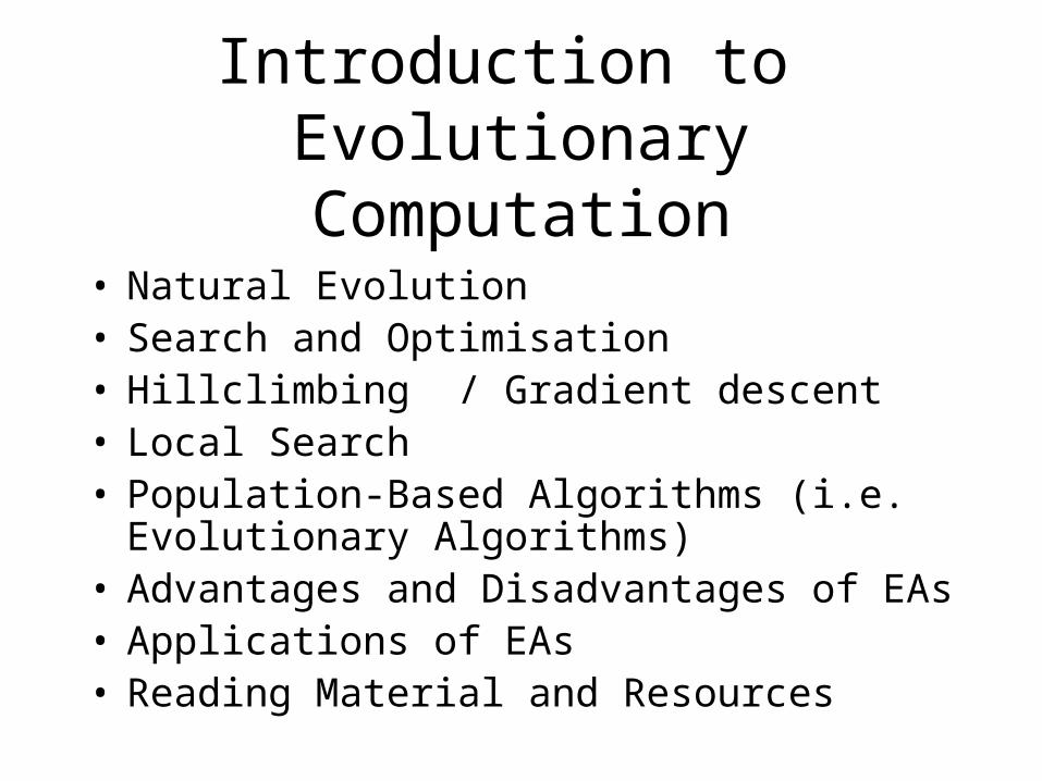
Introduction to Evolutionary Computation

• Natural Evolution• Search and Optimisation• Hillclimbing / Gradient descent• Local Search• Population-Based Algorithms (i.e. Evolutionary

Algorithms)• Advantages and Disadvantages of EAs• Applications of EAs• Reading Material and Resources

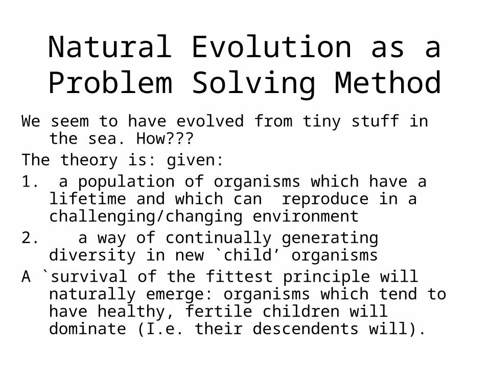
Natural Evolution as a Problem Solving Method

We seem to have evolved from tiny stuff in the sea. How???

The theory is: given:1. a population of organisms which have a lifetime and

which can reproduce in a challenging/changing environment

2. a way of continually generating diversity in new `child’ organisms

A `survival of the fittest principle will naturally emerge: organisms which tend to have healthy, fertile children will dominate (I.e. their descendents will).

Evolution/Survival of the Fittest In particular, any new mutation that appears in a child (e.g. longer

neck, longer legs, thicker skin, longer gestation period, bigger brain, light-sensitive patch on the skin, a harmless `loose’ bone, etc etc) and which helps it in its efforts to survive long enough to have children, will become more and more widespread in future generations.

The theory of evolution is the statement that all species on Earth have arisen in this way by evolution from one or more very simple self-reproducing molecules in the primeval soup. I.e. we have evolved via the accumulation of countless advantageous (in context) mutations over countless generations, and species have diversified to occupy niches, as a result of different environments favouring different mutations.

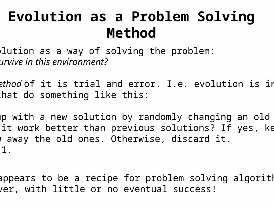
Evolution as a Problem Solving Method

Can view evolution as a way of solving the problem: How can I survive in this environment?

The basic method of it is trial and error. I.e. evolution is in the familyof methods that do something like this:

1. Come up with a new solution by randomly changing an old one. Does it work better than previous solutions? If yes, keep it and throw away the old ones. Otherwise, discard it. 2. Go to 1.

But this appears to be a recipe for problem solving algorithms whichtake forever, with little or no eventual success!

The Magic Ingredients

Not so – since there are two vital things (and one other sometimes useful thing) we learn from natural evolution, which, with a sprinkling of our own commonsense added, lead to generally superb problem solving methods called evolutionary algorithms: Lesson1: Keep a population/collection of different things on the go.

Lesson2: Select `parents’ with a relatively weak bias towards the fittest. It’s not really plain survival of the fittest, what works is the fitter you are, the more chance you have to reproduce, and it works best if even the least fit still have some chance.

Lesson3: It can sometimes help to use recombination of two or more `parents’ – I.e. generate new candidate solutions by combining bits and pieces from different previous solutions.

A Generic Evolutionary Algorithm Suppose you have to find a solution to some problem or other, and suppose,

given any candidate solution s you have a function f(s) which measures how good s is as a solution to your problem.

Generate an initial population P of randomly generated solutions (this is typically 100 or 500 or so). Evaluate the fitness of each. Then:

Repeat until a termination condition is reached:

1. Selection: Choose some of P to be parents

2. Variation: Apply genetic operators to the parents to produce some children, and then evaluate the fitness of the children.

3. Population update: Update the population P by retaining some of the children and removing some of the incumbents.

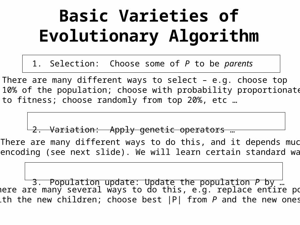
Basic Varieties of Evolutionary Algorithm

1. Selection: Choose some of P to be parents

2. Variation: Apply genetic operators …

3. Population update: Update the population P by …

There are many different ways to select – e.g. choose top 10% of the population; choose with probability proportionateto fitness; choose randomly from top 20%, etc …

There are many different ways to do this, and it depends much on theencoding (see next slide). We will learn certain standard ways.

There are many several ways to do this, e.g. replace entire populationwith the new children; choose best |P| from P and the new ones, etc.

Some of what EA-ists (theorists and practitioners) areMost concerned with:

How to select? Always select the best? Bad results, quickly Select almost randomly? Great results, too slowly

How to encode? Can make all the difference, and is intricately tied up with :

How to vary? (mutation, recombination, etc…) small-step mutation preferred, recombination seems to be a principled way to do large steps, but large steps are usually abysmal.

What parameters? How to adapt with time?

What are they good for ?

Suppose we want the best possible schedule for a university lecture timetable.

• Or the best possible pipe network design for a ship’s engine room

• Or the best possible design for an antenna with given requirements

• Or a formula that fits a curve better than any others

• Or the best design for a comms network in terms of reliability for given cost

• Or the best strategy for flying a fighter aircraft

• Or the best factory production schedule we can get,

• Or the most accurate neural network for a data mining or control problem,

• Or the best treatment plan (beam shapes and angles) for radiotherapy cancer treatment

• And so on and so on ….!

• The applications cover all of optimisation and machine learning.

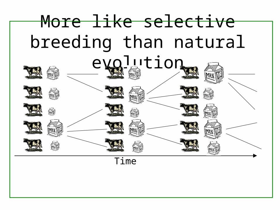
More like selective breeding than natural evolution

Time

Every Evolutionary Algorithm

Given a problem to solve, a way to generate candidate solutions, and a way to assign fitness values:

• Generate and evaluate a population of candidate solutions• Select a few of them• Breed the selected ones to obtain some new candidate

solutions, and evaluate them• Throw out some of the population to make way for some

of the new children. • Go back to step 2 until finished.

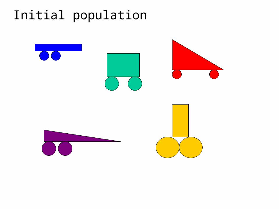
Initial population

Select

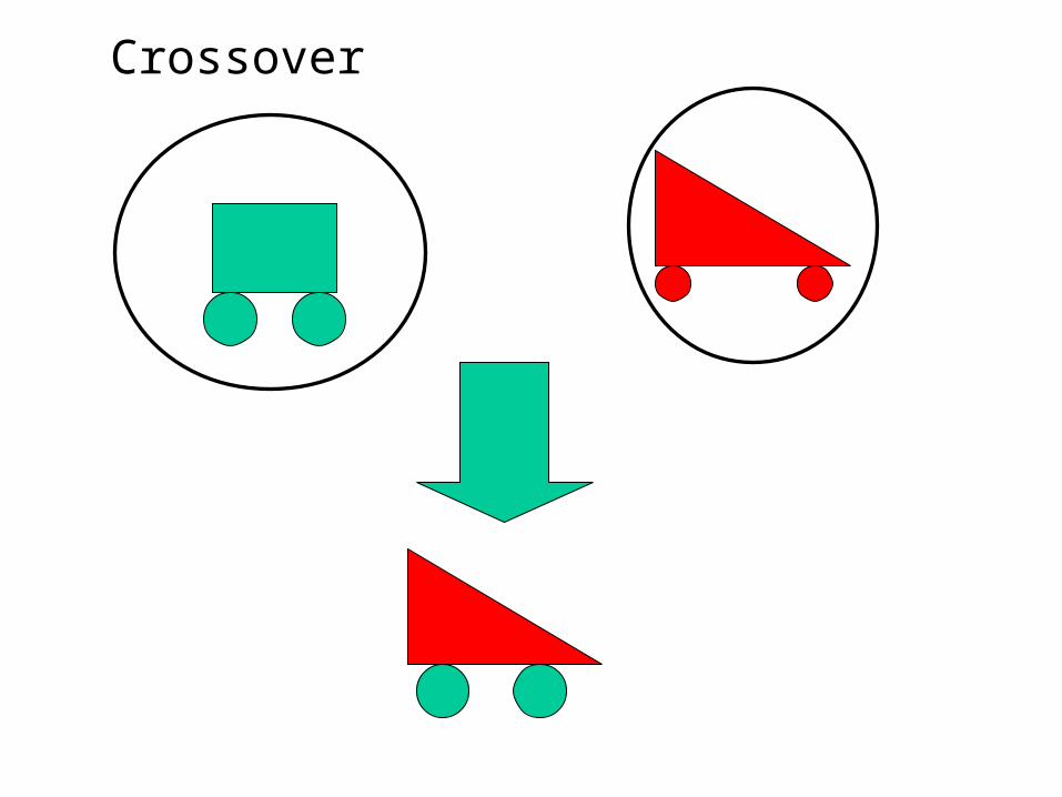
Crossover

Another Crossover

A mutation

Another Mutation

Old population + children

New Population: Generation 2

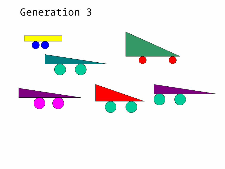
Generation 3

Generation 4, etc …

Fixed wheel positions, constrained bounding area, Chromosome is a series of slicesfitnesses evaluated via a simple airflow simulation

Bentley.s thesis work

Buy it

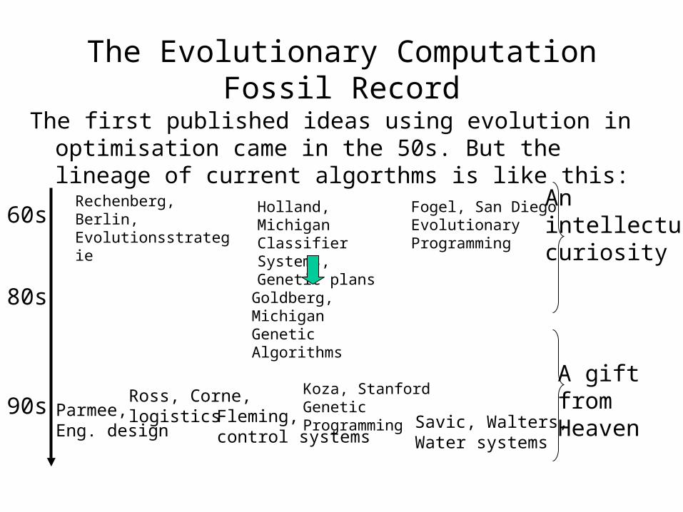
The Evolutionary Computation Fossil Record

The first published ideas using evolution in optimisation came in the 50s. But the lineage of current algorthms is like this:

Rechenberg, Berlin, Evolutionsstrategie

Holland, MichiganClassifier Systems, Genetic plans

Fogel, San DiegoEvolutionary Programming

Goldberg, MichiganGenetic Algorithms

Koza, StanfordGenetic ProgrammingParmee,

Eng. design Savic, Walters,Water systems

Ross, Corne, logistics Fleming,

control systems

60s

80s

90s

Anintellectualcuriosity

A gift fromHeaven

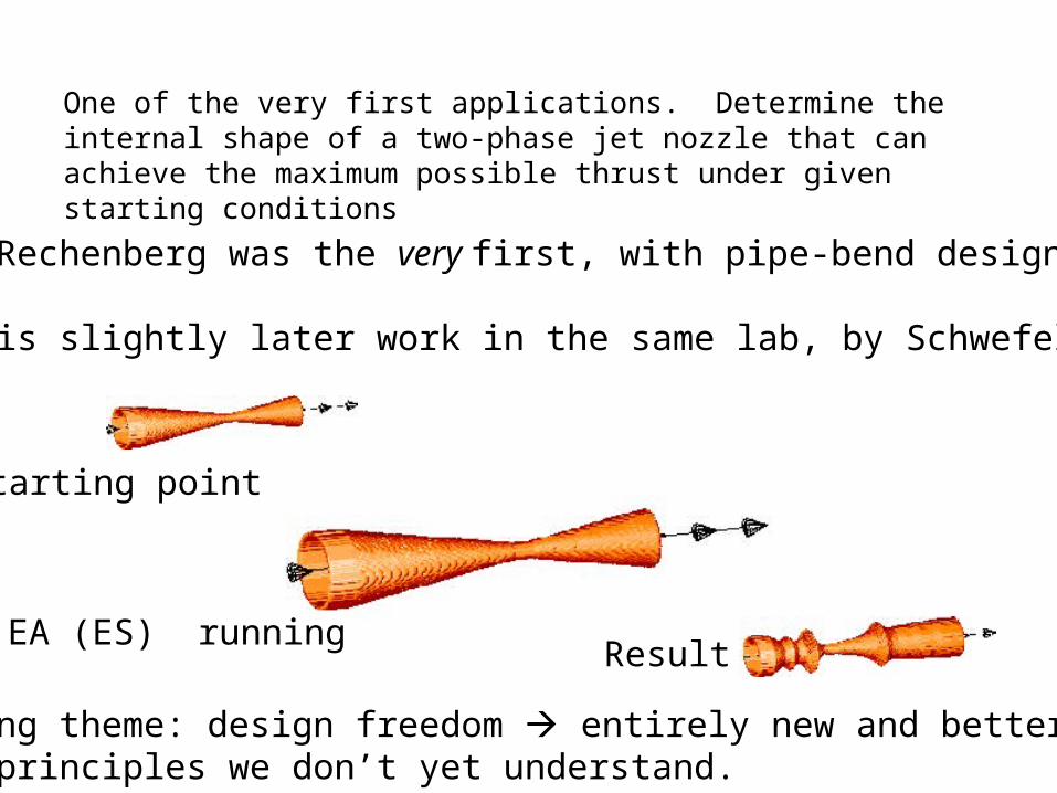
One of the very first applications. Determine the internal shape of a two-phase jet nozzle that can achieve the maximum possible thrust under given starting conditions

Ingo Rechenberg was the very first, with pipe-bend design

This is slightly later work in the same lab, by Schwefel

Starting point

EA (ES) runningResult

A recurring theme: design freedom entirely new and better designsbased on principles we don’t yet understand.

Some extra slides if time, illustrating some high-profile EAs

An innovative EC-designedPropellor from Evolgics GmbH,

Associated with Rechenberg’s group.

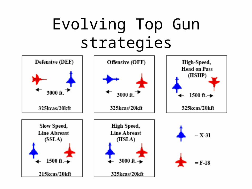
Evolving Top Gun strategies

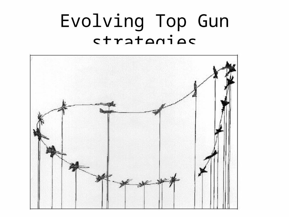
Evolving Top Gun strategies

NASA ST5 Mission had challenging requirements for antenna of 3 small spacecraft.

EA designs outperformed human expert ones and are nearly spacebound.

Credit Jason Lohn

Oh no, we knew something like this would happen

Credit Jason Lohn

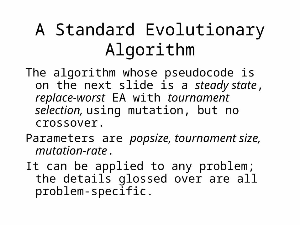
A Standard Evolutionary Algorithm

The algorithm whose pseudocode is on the next slide is a steady state, replace-worst EA with tournament selection, using mutation, but no crossover.

Parameters are popsize, tournament size, mutation-rate.

It can be applied to any problem; the details glossed over are all problem-specific.

A steady state, mutation-only, replace-worst EA with tournament selection

0. Initialise: generate a population of popsize random solutions, evaluate their fitnesses.

1. Run Select to obtain a parent solution X.2. With probability mute_rate, mutate a copy of X to obtain

a mutant M (otherwise M = X)3. Evaluate the fitness of M.4. Let W be the current worst in the population (BTR). If M

is not less fit than W, then replace W with M. (otherwise do nothing)

5. If a termination condition is met (e.g. we have done 10,000 evals) then stop. Otherwise go to 2.

Select: randomly choose tsize individuals from the population. Let c be the one with best fitness (BTR); return X.

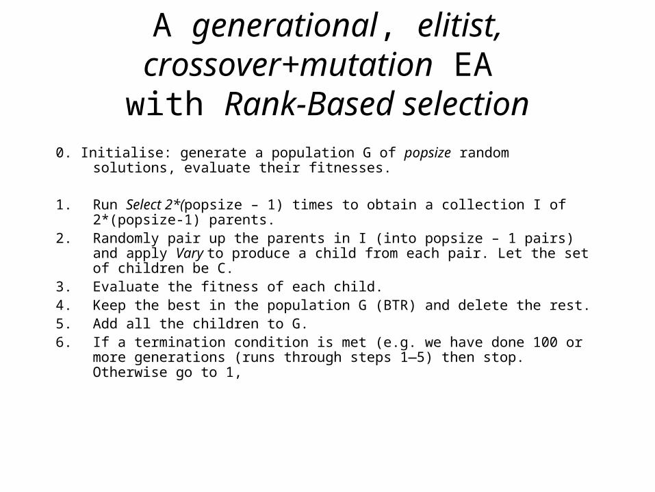
A generational, elitist, crossover+mutation EA

with Rank-Based selection0. Initialise: generate a population G of popsize random

solutions, evaluate their fitnesses.

1. Run Select 2*(popsize – 1) times to obtain a collection I of 2*(popsize-1) parents.

2. Randomly pair up the parents in I (into popsize – 1 pairs) and apply Vary to produce a child from each pair. Let the set of children be C.

3. Evaluate the fitness of each child.4. Keep the best in the population G (BTR) and delete the

rest. 5. Add all the children to G.6. If a termination condition is met (e.g. we have done 100

or more generations (runs through steps 1—5) then stop. Otherwise go to 1,

A generational, elitist, crossover+mutation EA with Rank-Based selection, continued …

Select: sort the contents of G from best to worst,

assigning rank popsize to the best, popsize-1 to the next best, etc …, and rank 1 to the worst.

The ranks sum to F = popsize(popsize+1)/2 Associate a probability Rank_i/F with each

individual i. Using these probabilities, choose one individual

X, and return X. Vary: 1. With probability cross_rate, do a crossover: I.e produce a child by applying a crossover operator to the two parents. Otherwise, let the child be a randomly chosen one of the parents. 2. Apply mutation to the child. 3. Return the mutated child.

Back to Basics

With your thirst for seeing example EAs temporarily quenched, the story now skips to simpler algorithms.

This will help to explain what it is about the previous ones which make them work.

The Travelling Salesperson Problem

An example (hard) problem, for illustration

The Travelling Salesperson ProblemFind the shortest tour through the cities.

AD E

CB

A B C D E

A 5 7 4 15

B 5 3 4 10

C 7 3 2 7

D 4 4 2 9

E 15 10 7 9

The one below is length: 33

Hillclimbing

0. Initialise: Generate a random solution c; evaluate its fitness, f(c). Call c the current solution.

1. Mutate a copy of the current solution – call the mutant mEvaluate fitness of m, f(m).

2. If f(m) is no worse than f(c), then replace c with m, otherwise do nothing (effectively discarding m).

3. If a termination condition has been reached, stop. Otherwise, go to 1.

Note. No population (well, population of 1). This is a very simple version of an EA, although it has been around for much longer.

Why “Hillclimbing”?

Suppose that solutions are lined up along the x axis, and that mutationalways gives you a nearby solutions. Fitness is on the y axis; this is a landscape

12

4

3

5, 8

67

9 10

1. Initial solution; 2. rejected mutant; 3. new current solution, 4. New current solution; 5. new current solution; 6. new current soln7. Rejected mutant; 8. rejected mutant; 9. new current solution,10. Rejected mutant, …

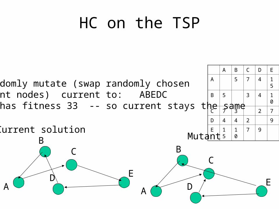
Example: HC on the TSP

We can encode a candidate solution to the TSP as a permutation

AD E

CB

A B C D E

A 5 7 4 15

B 5 3 4 10

C 7 3 2 7

D 4 4 2 9

E 15 10 7 9

D E

CB

Here is our initial random solution ABDEC withfitness 32

A

Current solutionMutant

HC on the TSP

AD E

CB

A B C D E

A 5 7 4 15

B 5 3 4 10

C 7 3 2 7

D 4 4 2 9

E 15 10 7 9

D E

CB

We randomly mutate (swap randomly chosenadjacent nodes) current to: ABEDCwhich has fitness 33 -- so current stays the same

A

Current solutionMutant

HC on the TSP

AD E

CB

A B C D E

A 5 7 4 15

B 5 3 4 10

C 7 3 2 7

D 4 4 2 9

E 15 10 7 9

D E

CB

We randomly mutate (swap randomly chosenadjacent nodes) current (ABDEC) to CBDEAwhich has fitness 38 -- so current stays the same

A

Current solutionMutant

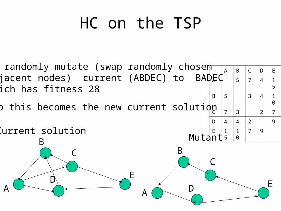
HC on the TSP

AD E

CB

A B C D E

A 5 7 4 15

B 5 3 4 10

C 7 3 2 7

D 4 4 2 9

E 15 10 7 9

D E

CB

We randomly mutate (swap randomly chosenadjacent nodes) current (ABDEC) to BADECwhich has fitness 28

A

Current solutionMutant

So this becomes the new current solution

HC on the TSP

AD E

CB

A B C D E

A 5 7 4 15

B 5 3 4 10

C 7 3 2 7

D 4 4 2 9

E 15 10 7 9

D E

CB

We randomly mutate (swap randomly chosenadjacent nodes) current (BADEC) to BADCEwhich also has fitness 28

A

Current solutionMutant

This becomes the new current solution

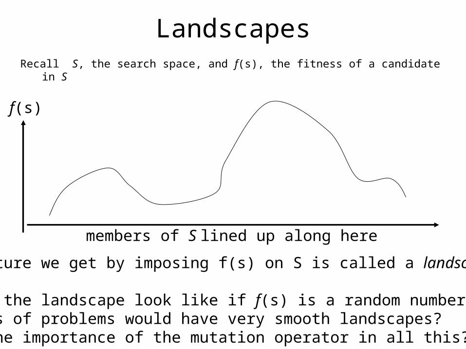
LandscapesRecall S, the search space, and f(s), the fitness of a candidate in S

f(s)

members of S lined up along here

The structure we get by imposing f(s) on S is called a landscape

What does the landscape look like if f(s) is a random number generator?What kinds of problems would have very smooth landscapes?What is the importance of the mutation operator in all this?

NeighbourhoodsLet s be an individual in S, f(s) is our fitness function, and M is

our mutation operator, so that M(s1) s2, where s2 is a mutant of s1.

Given M, we can usually work out the neighbourhood of an individual point s – the neighbourhood of s is the set of all possible mutants of s

E.g. Encoding: permutations of k objects (e.g. for k-city TSP) Mutation: swap any adjacent pair of objects. Neighbourhood: Each individual has k neighbours. E.g. neighbours of EABDC are: {AEBDC, EBADC, EADBC, EABCD, CABDE}

Encoding: binary strings of length L (e.g. for L-item bin-packing) Mutation: choose a bit randomly and flip it. Neighbourhood: Each individual has L neighbours. E.g. neighbours of 00110 are: {10110, 01110, 00010, 00100, 00111}

Landscape Topology

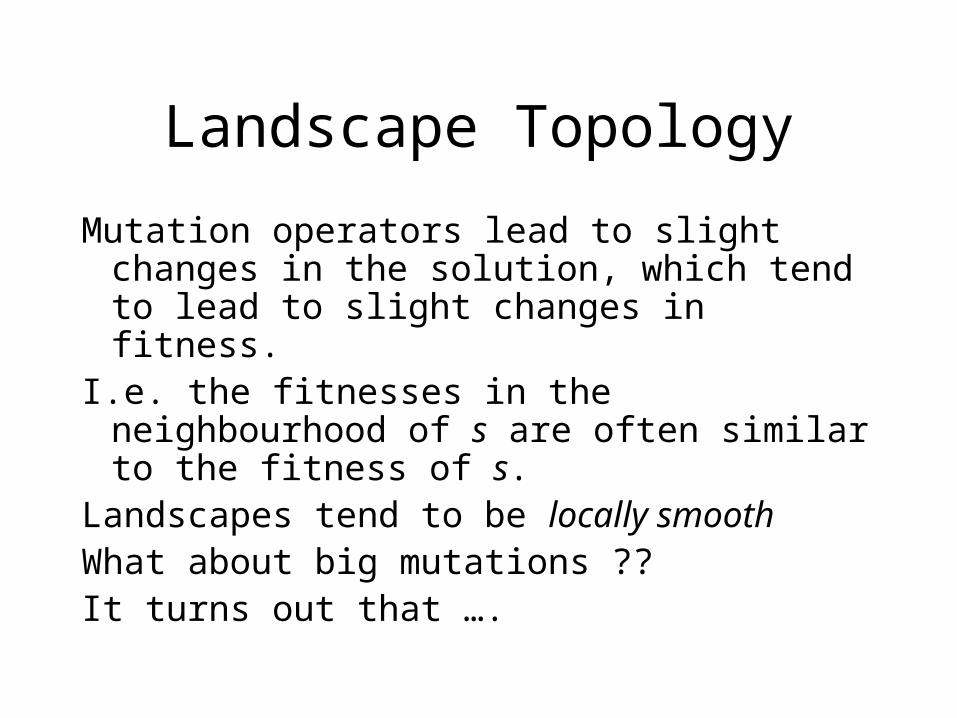
Mutation operators lead to slight changes in the solution, which tend to lead to slight changes in fitness.

I.e. the fitnesses in the neighbourhood of s are often similar to the fitness of s.

Landscapes tend to be locally smoothWhat about big mutations ??It turns out that ….

Typical Landscapes

f(s)

members of S lined up along here

Typically, with large (realistic) problems, the huge majority of thelandscape has very poor fitness – there are tiny areas where the decent solutions lurk.So, big random changes are very likely to take us outside the nice areas.

Typical Landscapes II

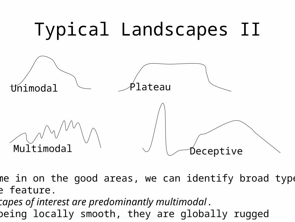
As we home in on the good areas, we can identify broad types of Landscape feature. Most landscapes of interest are predominantly multimodal.Despite being locally smooth, they are globally rugged

Unimodal Plateau

Multimodal Deceptive

Beyond Hillclimbing

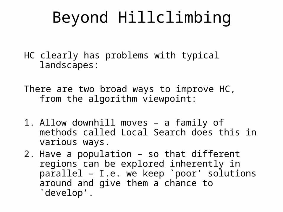
HC clearly has problems with typical landscapes:

There are two broad ways to improve HC, from the algorithm viewpoint:

1. Allow downhill moves – a family of methods called Local Search does this in various ways.

2. Have a population – so that different regions can be explored inherently in parallel – I.e. we keep `poor’ solutions around and give them a chance to `develop’.

Local Search

Initialise: Generate a random solution c; evaluate its fitness, f(s) = b; call c the current solution, and call b the best so far.

Repeat until termination conditon reached:1. Search the neighbourhood of c, and choose one, m Evaluate fitness of m, call that x.2. According to some policy, maybe replace c with x, and update c and b as appropriate.

E.g. Monte Carlo search: 1. same as hillclimbing; 2. If x is better, accept it as new current solution;if x is worse, accept it with someprobabilty (e.g. 0.1).

E.g. tabu search: 1. evaluate all immediate neighbours of c 2. choose the best from (1) to be the next current solution, unless it is`tabu’ (recently visited), in which choose the next best, etc.

Population-Based Search• Local search is fine, but tends to get stuck in local

optima, less so than HC, but it still gets stuck.• In PBS, we no longer have a single `current solution’,

we now have a population of them. This leads directly to the two main algorithmic differences between PBS and LS– Which of the set of current solutions do we mutate? We

need a selection method– With more than one solution available, we needn’t just

mutate, we can [mate, recombine, crossover, etc …] two or more current solutions.

• So this is an alternative route towards motivating our nature-inspired EAs – and also starts to explain why they turn out to be so good.

TSP, this time with an EA

A steady state EA with mutation-only, running for a few steps on the TSP example, with an unidentified selection method.

Running a Steady State EA -- TSPA B C D E

A 5 7 4 15

B 5 3 4 10

C 7 3 2 7

D 4 4 2 9

E 15 10 7 9

Let’s encode a solution as a permutation

Initial randomly generated pop of 5: ACEBD DACBE BACED CDAEB ABCEDEvaluation 32 33 28 31 28

Mutant of selected parent CDAEB ADCEB

Evaluation of mutant: 26

Mutant enters population, replacing worst

Running a Steady State EA -- TSPA B C D E

A 5 7 4 15

B 5 3 4 10

C 7 3 2 7

D 4 4 2 9

E 15 10 7 9

Generation 2 ACEBD ADCEB BACED CDAEB ABCEDEvaluation 32 26 28 31 28

Mutant of selected parent BACED BDCEA

Evaluation of mutant: 33

Mutant discarded– worse than current worst

Running a Steady State EA -- TSPA B C D E

A 5 7 4 15

B 5 3 4 10

C 7 3 2 7

D 4 4 2 9

E 15 10 7 9

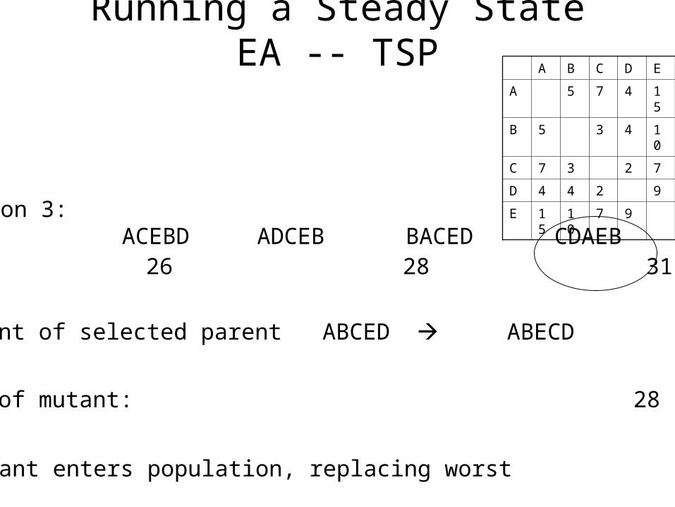
Generation 3: ACEBD ADCEB BACED CDAEB ABCEDEvaluation 32 26 28 31 28

Mutant of selected parent ABCED ABECD

Evaluation of mutant: 28

Mutant enters population, replacing worst

Running a Steady State EA -- TSPA B C D E

A 5 7 4 15

B 5 3 4 10

C 7 3 2 7

D 4 4 2 9

E 15 10 7 9

Generation 4: ABECD ADCEB BACED CDAEB ABCEDEvaluation 28 26 28 31 28

Mutant of selected parent ADCEB BDCEA

Evaluation of mutant: 33

Mutant is discarded

Running a Steady State EA -- TSPA B C D E

A 5 7 4 15

B 5 3 4 10

C 7 3 2 7

D 4 4 2 9

E 15 10 7 9

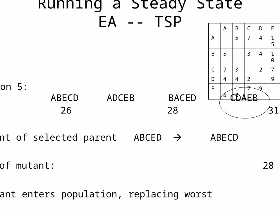
Generation 5: ABECD ADCEB BACED CDAEB ABCEDEvaluation 28 26 28 31 28

Mutant of selected parent ABCED ABECD

Evaluation of mutant: 28

Mutant enters population, replacing worst

Running a Steady State EA -- TSPA B C D E

A 5 7 4 15

B 5 3 4 10

C 7 3 2 7

D 4 4 2 9

E 15 10 7 9

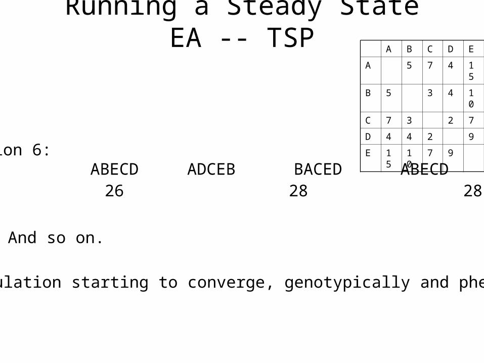
Generation 6: ABECD ADCEB BACED ABECD ABCEDEvaluation 28 26 28 28 28

And so on.

Note: population starting to converge, genotypically and phenotypically