PPN as Explosions: Bullets vs Jets and Nebular Shaping

arX

iv:0

707.

1641

v3 [

astr

o-ph

] 1

3 Ju

l 200

7

PPN as Explosions: Bullets vs Jets and Nebular Shaping

Timothy J. Dennis1, Andrew J. Cunningham1, Adam Frank1

[email protected]

Bruce Balick2, Eric G. Blackman1

and

Sorin Mitran3

ABSTRACT

Many proto-planetary nebulae (PPN) appear as narrow collimated structures

sometimes showing multiple, roughly aligned lobes. In addition, many PPN

flows have been shown to have short acceleration times. In this paper we explore

whether jet or “bullet” (a massive clump) models fit the observations of individual

collimated lobes adequately by comparing simulations of both radiatively cooled

(stable) jets and bullets. We find that the clump model is somewhat favored

over jets because (1) it leads to greater collimation of outflows (2) it accounts

better and more naturally for ring-like structures observed in the PPN CRL

618, and (3) it is more successful in reproducing the Hubble-flow character of

observed kinematics in some PPN. In addition, bullets naturally account for

observed multipolar flows, since the likely MHD launch mechanisms required to

drive outflows make multiple non-aligned jets unlikely. Thus we argue that PPN

outflows may be driven by explosive MHD launch mechanisms such as those

discussed in the context of supernovae (SNe) and gamma-ray bursts(GRB).

Subject headings: ISM:jets and outflows—planetary nebulae:general—planetary

nebulae:individual (CRL-618)—stars:AGB and Post-AGB

1Department of Physics & Astronomy, University of Rochester, Rochester, NY 14627

2 Department of Astronomy, University of Washington, Seattle, WA 98195

3 Department of Mathematics, University of North Carolina, Chapel Hill, NC 27599

– 2 –

1. Introduction

In the past decade, images of very young planetary nebulae (PNs) and proto-planetary

nebulae (PPNs) have revealed an unexpected diversity of morphological classes. Many of

these objects appear to exhibit a level of complexity that cannot be accounted for in terms

of the Generalized Interacting Stellar Winds model (GISW; Balick & Frank 2002 and ref-

erences therein). Of particular interest are objects exhibiting point-symmetric, multi-polar,

and “butterfly” morphologies, as well as bipolar and multi-polar objects exhibiting highly

collimated “jet-like” outflows.

The appearance of these collimated and sometimes multi-polar outflows in so many

PPNs has led to the suggestion that high-speed jets operate during the late asymptotic giant

branch (AGB) and/or post-AGB evolutionary phases of the central star (Sahai & Trauger

1998). While the GISW model can account for narrow jets (Icke et al. 1992; Mellema & Frank

1997; Borkowski, Blondin, & Harrington 1997), it assumes the winds are radiatively driven.

Radiative acceleration cannot however account for these flows since a number of observational

studies demonstrate a momentum excess such that a factor ∼ 103 exists between outflow

momentum observed and what can be attributed to stellar radiation pressure (Bujarrabal

et al. 2001). Moreover, it is difficult to attribute the degree of observed collimation to a

large-scale dust torus as is usually required in the GISW model. In addition, the problem of

accounting for the precession necessary for the production of point-symmetric flows remains

to be solved [for an accretion disk based model see Icke (2003)]. For these reasons, the

suggestion has been made that PPN jets and collimated outflows are magnetically driven

(Blackman et al. 2001a, 2001b; Frank & Blackman 2004; Matt, Frank, & Blackman 2006,

Frank 2006). Magnetically driven models couple rotation to a magnetic field. Jets therefore

are bound to flow along the rotational axis of the central object and it is difficult to see how

multiple jets of similar size can be driven by such a mechanism. We discuss these models

and this issue in more detail at the end of the paper.

Observationally, clumps and collimated flows occur in many stellar outflows though not

always together. The outflows in Wolf-Rayet (WR) nebulae are clumpy, but jets are not

observed. In young stellar objects (YSOs), jets and collimated bipolar outflows are quite

common, and while they can often be clumpy, the jet beams—distinct from the bow shocks

which they drive—are often apparent, stretching all the way back to the stellar source. In

mature PN, clumps are often seen [as in NGC 2392 (Eskimo), 6853 (Dumbbell) and NGC

7293 (Helix)]. Fully articulated jets are however very rare. We note that ionization shadows

and “mass loaded” flows behind clumps can give the appearance of jets. In some mature PN

such as the Cats Eye nebula, structures appear (some of which fall under the term FLIERS)

which may be the remnants of poleward-directed flows. In HST images of many PPNs, the

– 3 –

outlines of reflected light are often bipolar, but within these boundaries the illuminated gas

seems irregular. Thin jets (as opposed to thin finger-shaped lobes) are rarely seen directly

except (perhaps) in 0H231.8+04.2 (Calabash) . However, pairs or sets of knots lying along

or near the apparent symmetry axes are not unusual (M1-92, IRAS 20028 +3910, IRAS

16594-3656, Hen 3-1475). Thus the creation of continious jets as in the case of YSOs does

not seem to be the norm in PN and PPN.

Clumps or “bullets” driven into the surrounding media have been found to be an effective

explanation for some stellar outflow structures. In Poludnenko, Frank, & Mitran (2004) the

authors modeled the strings of η Car as bullets of high speed material ejected by the star.

The simulations showed that long, thin morphologies similar to jets were readily obtained

along with multiple rings associated with vortex shedding and the break-up of the clump.

The authors suggested that such “impulsive” models may be useful in PPNs as well. Such

a scenario is very different from the jet-driven explanation for PPN/PN. In this paper we

seek to explore the usefulness of the clump picture.

Soker (2000) has analytically explored the role of jets in PNs. In the excellent study

of Lee & Sahai (2003), simulations of jets as the drivers of PPNs were presented, including

detailed comparisons with observations. Our goals in this paper are more modest. In what

follows we take a first step in the exploration of the clumps vs. jets issue by examining

2-dimensional and 3-dimensional pairs of simulations, with each pair consisting of either a

steady jet impinging upon a circumstellar gaseous medium, or a clump of gas which is fired

ballistically through the same medium along a trajectory corresponding to the direction of

flow in the steady jet 1. Both the jet and the clump are assumed to be magnetically launched

though no attempt to model the launch mechanism is made here, and the simulations are

purely hydrodynamic. For the present, we are merely interested in examining how the clump

and jet differ in their effect on the surrounding circumstellar medium. As we will show, the

jet and clump models show differences which require further study, but the clumps provide

at least as good, or better, an account of key observational characteristics. Given the fact

that in some cases multiple outflows are seen in a single object (such as CRL 618), the clump

model may be more plausible since what are often interpreted as multiple “jets” could instead

arise naturally from the fragmentation of an explosively driven polar directed shell. We note

here that none of the widely accepted magnetically launched outflow models would create

continuous multiple jets of similar or equal age driven in slightly different directions.

We note also that new models of binary stars in the context of PN’s (Nordhaus &

1In a related study Raga et al.(2007) have also recently presented a model of the “3D structure of a

radiative, cosmic bullet flow.”

– 4 –

Blackman 2006, Nordhaus, Blackman & Frank 2007) show the extent to which envelope

ejection can be shaped by gravitational interactions. In Nordhaus & Blackman 2006 Common

Envelope scenarios which lead to aspherical mass loss (including disk creation and possible

MHD launching) were articulated. In Nordhaus, Blackman & Frank 2007 Common Envelope

models were explored as the source of differential rotation in the primary which could drive

strong dynamo supported magnetic fields. These models showed that while single stars may,

in some cases, be able to support a strong field over AGB timescales, binary interactions

were highly effective at creating the fields needed to power PPN outflows at the evolutionary

moment when they will be required. As we will see, such models provide strong theoretical

support for the scenario we argue for in this paper.

In section 2 we provide information concerning the numerical methods used, details of

the jet and clump models, and a discussion of the initial conditions. In section 3 we discuss

the results of our simulations and in section 4 we summarize our conclusions.

2. Computational Methods and Initial Conditions

We have carried out two pairs of hydrodynamic simulations (one “medium-resolution”

3D pair and one “high-resolution” 2.5D pair). Each pair consists of a jet and clump re-

spectively with each parameterized to be as similar to one another as possible. Specific

parameter values for the jet, clump, and ambient medium for each simulation are given in

table 1. The simulations are performed using the AstroBEAR code which is an extension of

the BEARCLAW adaptive mesh refinement (AMR) package for solving conservation laws.

[For a detailed description of the AstroBEAR package see section 3 of Cunningham Frank

& Blackman (2006).] The domain is a rectangular box with a square cross-section and with

the x-axis chosen to intersect the center of the left square face of the domain. The origin

of coordinates is placed at this point of intersection. The clump and jet are launched along

the x-axis and placed so that their centers coincide with it. The jet was modeled in 3D with

a circular cross-section of radius rj (in 2.5D the jet cross-section reduces to a line-segment

of length 2rj and a thickness of one computational cell). The jet was launched into the

domain from a set of fixed cells along the domain boundary. To prevent the expansion of

the jet inflow boundary with time, a ring of zero velocity and with outer radius 1.125r0 was

maintained around the jet-launching region. The velocity profile of the jet was smoothed

about a nominal value vj,0 according to

vj = vj,0

[

1 − (1 − s)

(

r

r0

)2]

, (1)

– 5 –

where s is a shearing parameter taking values between 0 and 1 and for the jet simulation

presented here is set equal to s = 0.9. The clump was modeled in 3D as a spherical over-

density of radius rc = rj. (The sphere reduces to a circle in 2.5D.) Its initial position in the

domain is chosen so that its center is located at the point

rc,0(x, y, z) = (2rc, 0, 0), (2)

and the density of the clump as a function of location within the clump is

nc(r) = na(r) + n0

[

1 −( |r − rc,0|

r0

)2]

, (3)

where

na(r) = min

(

n0,n0r

20

r2

)

, (4)

is the ambient number density profile in regions of the domain unoccupied by jet or clump

gas, and where r2 = x2 + y2 + z2, n0 is the nominal ambient number density, and r0 is a

characteristic length taken to be equal to the jet or clump radius. The 3D (2.5D) simulations

are carried out on a base grid with a resolution of 6 (12) cells per jet/clump radius and with

two levels of AMR refinement providing an effective resolution of 24 (48) cells per jet/clump

radius. In all cases, radiative cooling is modeled using the atomic line cooling function

of Delgarno & McCray (1972), and we do not attempt to follow the detailed ionization

dynamics or chemistry of the cooling gas. Given that both models give rise to similarly

expanding shells of shock-heated gas we do not expect this simplification to materially affect

our conclusions.

– 6 –

Model Parameter Value (2.5D) Value (3D)

Jet Radius, rj . . . . . . . . . . . . . . . . . 500 AU 500 AU

Computational cells per rj . 48 24

number density, nj . . . . . . . . . 500 cm−3 500 cm−3

peak velocity, vj,0 . . . . . . . . . . 100 km s−1 100 km s−1

Temperature, Tj . . . . . . . . . . . 200 K 200 K

Nominal ambient density, na 500 cm−3 500 cm−3

Ambient temperature, Ta . . 200 K 200 K

Shear parameter s . . . . . . . . . 0.9 0.9

Clump Radius, rc . . . . . . . . . . . . . . . . . 500 AU 500 AU

Computational cells per rc . 48 24

nominal number density, no 500 cm−3 500 cm−3

velocity, vc . . . . . . . . . . . . . . . . . 100 km s−1 100km s−1

Temperature, Tc . . . . . . . . . . . 200 K 200 K

Nominal ambient density, na 500 cm−3 500 cm−3

Ambient temperature, Ta . . 200 K 200 K

Table 1: Simulation Parameters

– 7 –

3. Results: Morphology

Results of our simulations are presented in figures 1−6. In Figures 1 and 2 we present the

results of medium resolution, (24 cells per radius), 3D simulations of one jet and one clump

respectively. The length of the domain in these simulations is 20 computational units with

one computational unit corresponding to a physical scale of 500 AU. (One computational

unit is also the value chosen for the radii of the jet and clump.) In each figure the upper

image shows a plot of emission integrated along the line of sight which in the case of these

figures is perpendicular to the plane of the image. The lower image in each figure is a plot

of the logarithm of density in a plane coincident with the x-y plane. The images show the

jet and clump near the end of their respective runs at time t ≃ 498 yr for the case of the

clump and at time t ≃ 636 yr for the case of the jet. The resolution is seen to be sufficient

to capture vortex-shedding events in both simulations. It is also evident from these images

that while one can easily distinguish jet from clump in the density maps, the emission maps

are quite similar. We note that the clump gives rise to a somewhat more collimated flow,

while the jet bow shock expands laterally at a greater rate than the clump bow shock. The

jet also lags behind the clump in its forward motion. This is likely due to the streamlining

that occurs as the head of the clump is reduced in size as material is ablated away via its

interaction with the ambient medium.

Due to limits on computational resources, it was necessary to impose limits on the

resolution and run time of the 3D simulations from which the images in figures 1 and 2 are

taken. The simulations end just as the vortex-shedding events begin to have an interesting

effect on the nebular environment. To explore this stage further we carried out the second

pair of 2.5D simulations mentioned above. In these high-resolution simulations, the effective

resolution was doubled to 48 cells per jet/clump radius, the length of the domain was doubled,

and the transverse dimensions of the domain were enlarged in an attempt to accomodate

the lateral expansion of the jet/clump bow shock (this latter adjustment was successful only

for the case of the clump). Results from these simulations are presented in figures 3 through

6. In figures 3 and 4 we again present images of the logarithm of density for the jet and

clump respectively—this time reflected about the axis of symmetry. Both figures show the

simulations at various stages of the flow. We observe that the differences found between the

two models in the 3D simulations—i.e. the faster domain crossing time and the higher degree

of collimation exhibited by the clump—are seen again in these images. The vortex shedding

however, is now captured with greater clarity for both jet and clump, and we begin to see

significant qualitative differences in the manner in which these events unfold. In particular

we note that shedding events are much more frequent in the case of the clump. These results

mirror those found by Poludnenko, Frank & Mitran (2004). It is noteworthy that their study

used a different integration scheme than used here. AstroBEAR has a number of schemes

– 8 –

built into it and in the Poludnenko study a Wave Propagation scheme was used (LeVeque

1997), while here a MUSCL-Hancock method is used. The fact that the basic morphology

of clumps driving bow shocks dominated by vortex shedding events is recovered using both

schemes gives us confidence in this aspect of the dynamics.

3.1. Morphology

To get a better sense of how the differences between the models might appear observa-

tionally, we present integrated emission maps for the jet and clump respectively in figures

5 and 6. These figures were produced by calculating the effect on the line-of-sight emission

resulting from a rotation of the cylindrically symmetric data set about the axis of symme-

try. The intensity shown, which does not distinguish among cooling lines, was determined

according to:

Ii,j,k = Σkn2i,j,kΛ(Ti,j,k), (5)

where i,j, and k refer to the x,y and z directions in the final data cube created by rotating

n(r, z) and T (r, z) about the axis of symmetry, and Λ is the cooling function. The images

shown correspond to the final frames in each of figures 3 and 4 respectively. Each figure

provides two views of the data: one in which the angle of inclination of the symmetry axis

with respect to the image plane, θ, is 0◦; and one in which it is 20◦. One difference between

the jet and clump cases appears in the shape of the head of the bow shock. A clump has a

finite reservoir of mass which interacts with the ambient medium. As the clump propagates

down the grid, it drives a (bow) shock wave into the ambient medium. A second shock passes

through the clump heating and compressing it. When cooling is present this ”transmitted

shock” first leaves the clump flattened. As material is then ablated away via the interactions

with the ambient medium the remaining clump material becomes dense and streamlined in

the direction of propagation. At later times in the simulation the dense core of the clump

drives a V - shaped bow shock head. In the case of a jet the situation is different. The jet

head drives a bow shock into the ambient medium and transmitted shock, called a jet shock,

propagates back into the jet material. Decelerated jet material flows transverse the these

shocks inflating a cocoon behind the wings of the bow shock. Unlike the clump however,

there is always more high speed material behind the jet shock/bow shock pair to resupply

the interaction. Thus with material continuously flowing into the cocoon, the bow shock

head remains wider and takes on a flatter more U - shaped configuration. Such a distinction

between V - and U - shaped flows may be important in comparing with observations. We

note that both the 2.5D and 3D simulations both show this difference. We note however

that the axial symmetry will tend to enhance features on the axis. Our 3D runs do not yet

have the resolution to accurately track the break-up of the clump. Thus the V and U bow

– 9 –

shock head distinction must be considered less than conclusive and await further study.

Vortex shedding provides another morphological distinction. In the case of the clump,

the relatively frequent shedding events have led to a series of thin, irregularly spaced rings of

enhanced intensity centered about the symmetry axis. These are reminiscent of the ring-like

structures observed in some collimated PPN outflows [see for example Trammell & Goodrich

(2002)]. The shedding events occurring in the jet simulation lead to similar structures, but

these are less frequent and somewhat more band-like in character. The qualitative differences

in the manner in which these rings form in the outflows depending on whether one models

them as jets or clumps might suggest a means of distinguishing between the two models in

observations. One must, once again, be careful not to over-interpret these results due to

limits on the resolution and the fact that these simulations are 2.5D. We thus conclude that

the high-resolution 2.5D simulations lend weight to the assertion that clumps and/or jets

can account for observed ringed structures, but neither can be ruled out as a model for the

collimated outflows observed in the environments of PPNs. In the meantime, we note that

this conclusion in itself is important with respect to PPN studies as we will discuss in the

last section.

It is also noteworthy that Lee & Sahai (2003) attempted to model the rings via a pulsed

jet. Each ring became associated with an “internal working surface” where faster moving

material swept over slower moving material. The internal shocks lead to transverse motions

of shocked material which impinge upon the bow shock. As might be expected, the strength

of the emission from these shocks decreased as the pulse traveled down the length of the

beam. Such dimming of the rings with distance from the source is not what is observed in

CRL 618. The clump on the other hand produces the opposite kind of pattern, as ablation

events on the clump lead to rings that are bright closer to the head of the bow shock.

3.2. Kinematics

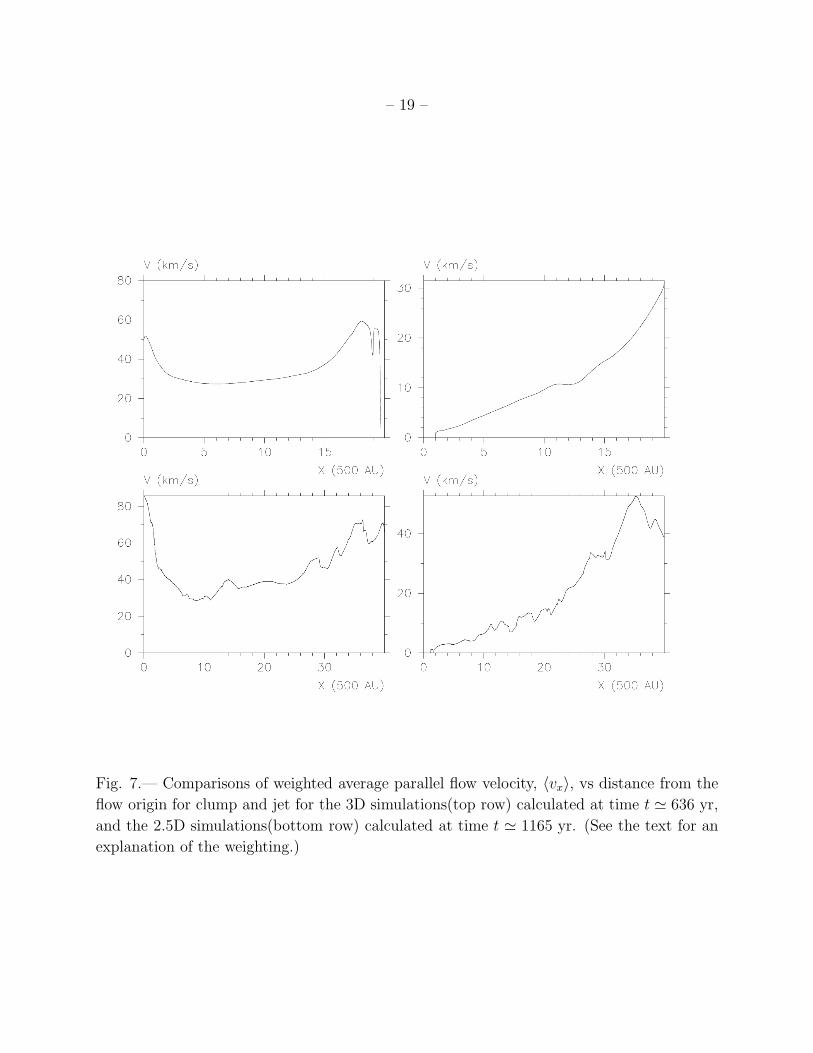
In addition to comparisons of morphology, it is also important to consider the flow

kinematics, since observed flows are often seen to exhibit “Hubble-flow” characteristics—

that is, the flow velocity is observed to increase linearly with respect to distance from the

flow origin. To address this issue we present in figure 7, plots of the x-component of the

flow velocity averaged over the directions transverse to the flow 〈vx〉. Velocity tracers were

not used in our simulations. In order, therefore, to differentiate between mildly perturbed

ambient gas, and gas that is fully involved in the flow, values of velocity . 0.01v0 were

ignored, where v0 is the initial velocity of the clump or jet gas. The top row of the figure

shows, from left to right, the results for the 3D jet and clump respectively while the bottom

– 10 –

figure shows the results for the 2.5D jet and clump. The data for these plots are taken from

times near the end of the simulation when the flows have crossed most of the domain. In

the two plots involving clumps, there are large regions of the flow for which the variation

of velocity with distance is roughly linear. The jets on the other hand, fail to model this

behavior altogether. Comparison of the 3D clump plots to the 2.5D case yields an interesting

result. Recall that the first vortex-shedding events in both clump and jet were observed to

occur in the 3D simulations shortly before the end of the simulation. Because of this they do

not have time to perturb the flow in a way that might be noticeable in these plots. However,

when we examine this phenomenon kinematically in the extended spatial domain allowed by

the 2.5D simulation, we find that while the vortex shedding events, appear to perturb the

kinematics of both jet and clump, these perturbations do not alter the overall qualitative

character of the flows in either case.

To further examine the kinematics of our simulated flows, we have also produced a set

of synthetic position-velocity (PV) diagrams for the 2.5D simulations. These are presented

in figure 8. Once again, as in figures 5 and 6 we present our results in pairs corresponding to

values of 0◦ and 20◦ for the angle of inclination, θ, of the flow symmetry axis with respect to

the image plane. These plots were produced by calculating the velocity structure along the

line of sight and with the “slit” placement taken to be along the projected axis of symmetry.

Results for the jet are given in the first row of the figure, and results of the clump are given

in the second row. In these images, the difference between the clump and jet are even more

striking. For either angle of inclination, the velocity structure of the jet cannot be said to

be even approximately Hubble-like. The clump however, continues to exhibit line-of-sight

velocity structure indicative of a linear increase with distance along the projected direction

of flow. The effect is particularly apparent in the case of the flow which is inclined with

respect to the image plane. These results, and those of figure 7 suggest that it may be

possible to distinguish outflows from steady jets from those from explosive events through a

careful examination of their kinematics.

One caveat which must be considered in these results is the role of emission. Because

our models do not track emission from individual species we cannot separate the emission at

the bow shock from that within the jet or from the shocked jet material. In Ostriker et al.

(2001), a model for the emission from a jet-driven bow shock was presented which showed

a characteristic spur pattern in synthetic PV diagrams. The spur exhibits a rapid drop in

velocity away from the tip of the bow shock. Lee & Sahai (2003) found a range of patterns

in their jet simulations which in some cases took on the spur morphology. Thus our results

are suggestive of the differences between jets and clumps and indicate that clumps appear

to be better, in general, at recovering quasi-linear increases in velocity along the nebular

outflow lobe.

– 11 –

3.3. Kinematic Models

In order to interpret our results we consider the time-dependent distortion of the clump

gas during the evolution of the outflow. Strongly radiative, hypersonic clouds of any geometry

will be rapidly compressed into a thin ballistic sheet after ejection by the outflow progenitor.

We therefore consider the motion of a cylindrically symmetric disk with surface density χ(r)

and velocity v(r, t) where v(r, 0) = v◦ to model the time-dependent evolution of the clump

gas. The equation of motion for a differential ring of the disk under the ram pressure of the

ambient gas of density ρ is given by:

ρv2(r, t) = −χdv

dt. (6)

Because the outflow bow shock is convex, most of the outflow-entrained ambient gas will be

swept outside of the path of the clump into the bow shock. We therefore neglect accretion

of ambient material onto the clump and the kinematics of ambient material ejection in this

model. Because the disk is hypersonic in a strongly cooling environment, we consider the

model disk to be ballistic, neglecting pressure forces. For simplicity we also take the density

of the ambient gas to be constant. Thus the equation of motion for a differential ring of

clump gas with radius r integrates to:

v =v0

1 + ρv0t/χ. (7)

The distance traversed by the ring is given as:

L(χ, t) =

∫ t

0

v(t)dt =χ

ρln

[

1 +ρv0t

χ

]

. (8)

The quantities v, t, and L, all refer to the same ring. What differentiates one ring of

material from another is the parameter r. Now at some late time t, we imagine the rings

to have been distributed over the length of the outflow with this distribution depending on

r. For this fixed value of t, we are interested plotting the velocity of each ring against its

corresponding distance. The r-dependence of v and L enter into the expressions for these

quantities through the surface density χ. We therefore model χ by assuming that the clump

of gas from which our disk formed was initially spherical, of constant volume mass density

σ, and compressed in such a way that all material within the volume of the clump and lying

along a given line passing through the clump in the direction of its motion remains on this

line after compression. Then,

χ(r) = 2σr0

√

1 − (r/r0)2, (9)

– 12 –

where r0 is the radius the clump/disk. Introducing the dimensionless quantities:

r =r

r0

, (10)

v =v

v0(11)

t =ρv0t

2σr0(12)

and,

L =ρ

2σr0

L, (13)

our parametric equations are:

v =

[

1 +t√

1 − r2

]−1

, (14)

and

L =√

1 − r2 ln

[

1 +t√

1 − r2

]

. (15)

The value of t is chosen by assuming σ & 2ρ, and by noting that at late times v0t & r0.

In our 2.5D simulations we have v0t/r0 ∼ 4t ≃ 20 making t ≃ 5. Figure 9 shows a plot of

v vs L in astronomically relevant units with this choice of t. For purposes of comparison,

a line with an appropriately chosen slope and intercept is plotted as well. In spite of the

simplicity of our analytical model, a comparison of this plot with the upper-right-hand plot

of figure 7 reveals good agreement between the two. Both curves exhibit a small concave

curvature for small L while becoming increasingly linear with increasing L (the downward

turn in the 2.5D simulation-based plot results from extending the plot into regions not yet

reached by the clump). We also find that the range of L-values over which the curve shows

linear behavior increases for increasing t, implying that a correlation between the kinematical

ages of PPN outflows and the extent to which they are observed to exhibit Hubble-flow. We

take this calculation as further evidence that our simulations are accurately capturing the

dynamics of the flow and the relevance of bullet models for PPN.

– 13 –

Fig. 1.— 3D Jet at time t ≃ 636 yr, top: integrated emission assuming atomic line cooling;

bottom, base-ten logarithm of density.

– 14 –

Fig. 2.— 3D clump at time t ≃ 498 yr, top: integrated emission assuming atomic line

cooling; bottom, base-ten logarithm of density.

– 15 –

Fig. 3.— Density of 2.5D Jet at times t ≃ 336, 628, 896, and 1165 yr. The data is shown

here reflected about the axis of symmetry.

– 16 –

Fig. 4.— Density crosscut of 2.5D Clump at times t ≃ 208, 477, 753, and 1082 yr. The data

is shown here reflected about the axis of symmetry.

– 17 –

Fig. 5.— Integrated emission of 2.5D Jet at time t ≃ 1132 yr. The data is shown here

rotated about the axis of symmetry and with angles of inclination of the symmetry axis with

respect to the image plain of θ = 0◦(top), and θ = 20◦(bottom).

– 18 –

Fig. 6.— Integrated emission of 2.5D Clump at time t ≃ 1082 yr. The data is shown here

rotated about the axis of symmetry and with angles of inclination of the symmetry axis with

respect to the image plain of θ = 0◦(top), and θ = 20◦(bottom).

– 19 –

Fig. 7.— Comparisons of weighted average parallel flow velocity, 〈vx〉, vs distance from the

flow origin for clump and jet for the 3D simulations(top row) calculated at time t ≃ 636 yr,

and the 2.5D simulations(bottom row) calculated at time t ≃ 1165 yr. (See the text for an

explanation of the weighting.)

– 20 –

Fig. 8.— Position-velocity diagrams at time t ≃ 1082 yr for the 2.5D Jet (top row) and the

2.5D Clump (bottom row) assuming inclination angles of θ = 0◦(left) and θ = 20◦(right).

– 21 –

Fig. 9.— V (r) vs L(r) for t = 5. See section 3.3 for an explanation of this figure.

– 22 –

4. Discussion and Conclusions

In this paper we have examined the results of two pairs of simulations intended to model

the gross morphological and kinematical properties of PPNs. Our primary purpose was to

ask not if we could distinguish between jet and clump models, but instead to ascertain if

clump models could perform equally well at recovering these properties. Below we explain

the justification for this more explicitly and present the conclusion of our study. As was

discussed in the introduction, MHD models of PN shaping have been explored by a variety

of authors and in a variety of forms. As we will explain below, it is the imperative of MHD

models, particularly magneto-centrifugal launch and collimation scenarios, which motivate

this paper.

Two distinct classes of model for the magnetic shaping of winds in PNs and PPNs have

been suggested to date. First there is the Magnetized Wind Bubble (MWB) model, originally

proposed by Chavalier & Luo (1994) and studied numerically by Rozyczka & Franco (1996)

and Garcia-Segura et al. (1999). In these models, an initially weak toroidal magnetic field

is embedded in a radiatively-driven wind. This configuration has been shown capable of

accounting for a wide variety of outflow morphologies including highly - collimated jets.

These models clearly demonstrate the importance of magnetic fields. They cannot however

account for the excess momentum in the flows (Bujarrabal et al. 2001) because of the weak

fields which simply ride along in a radiatively-driven wind.

The other class of model invokes so-called Magnetocentrifugal Launching (MCL; Bland-

ford & Payne 1982; Pelletier & Pudritz 1992). This paradigm has, for many years, been

explored as the mechanism driving jets in young stellar objects (YSOs), micro-quasars and

active galactic nuclei (AGNs). The MCL paradigm assumes the presence of a rotating central

gravitating object (which may or may not include an accretion disk). In the case of a disk,

plasma is threaded by a magnetic field whose poloidal component is in co-rotation with the

disk. Disk-coronal gas is then subject to centrifugal force which accelerates the gas flinging

it out along field lines. The magnetized plasma eventually expands to a configuration where

the toroidal component of the field dominates and hoop stresses collimate the flow. Thus

the MCL paradigm accounts for both the origin of the wind and the means of collimation.

The success of the MCL paradigm in modeling jets associated with YSOs and AGNs has

led some authors to suggest applying the idea in the context of PNs and PPNs (Blackman et

al. 2001a, Frank & Blackman 2004,). Most recently it has been shown that the observed total

energy and momentum in PPNs can be recovered with disk wind models using existing disk

formation scenarios via binary interaction (Frank & Blackman 2004 and references within).

Most theoretical investigations of the MCL paradigm assume a steady-state flow. Ob-

– 23 –

servations suggest however, that acceleration times for the flows are as much as an order of

magnitude shorter than typical kinematical PPN ages (Bujarrabal et al. 2001). This implies

that the mechanism responsible for the observed flows may operate explosively, i.e. the time

over which the mechanism acts is short compared to the lifetime of the flow. Moreover, it

has been suggested by Alcolea et al. (2001) that such a scenario would also provide the

most straightforward explanation for the “Hubble law” kinematics observed in some PPN

outflows (Balick & Frank 2002; Bujarrabal, Alcolea, & Neri 1998; Olafsson & Nyman 1999).

The MCL paradigm can act transiently however, when linked with the rapid evolution of its

source, as for example in the case of the proposed mechanisms for gamma-ray bursts (GRBs;

Piran 2005) and Supernovae (SNe). This scenario has been investigated by a number of

authors (Kluzniak & Ruderman 1998; Wheeler et al. 2002; Akiyama et al. 2003; Blackman

et al. 2006). In these scenarios differential rotation twists an initially weak poloidal field

thereby generating and amplifying a toroidal field. When the toroidal component reaches a

critical value it drives through the stratified layers of the collapsing core carrying trapped

material with it. The hoop stresses associated with such a field also serve to collimate the

flow.

Recently Matt, Frank, & Blackman (2006) examined numerically a simplified version of

this idea which was originally suggested for PPN in Blackman et al. 2001b. In these studies

the authors began with a gravitating core threaded by an initially poloidal field set rotating

at 10% of the escape speed within an envelope of ionized gas. As the simulation progressed,

the resulting toroidal field was sufficiently strong to drive a complete and rapid expulsion

of the gaseous envelope. Since the initial conditions assumed in Matt, Frank & Blackman

(2006) are applicable to either a young PPN or a collapsing protopulsar, it is reasonable to

ask whether such transient events are occurring in the early stages of the formation of PNs,

and if such events can serve as well as steady-state jets can in accounting for the complex

morphologies observed in such systems. We note that these classes of model are sometimes

referred to as “magnetic towers” or “springs” because it is the gradient of toroidal field

pressure which drives the outflow. Again we note that the magnetic fields needed for our

scenario can be delivered by binary interactions as has been demonstrated by Nordhaus &

Blackman 2006 and Nordhaus, Blackman & Frank 2007.

There is growing evidence to suggest that magneto-centrifugal launch models are appro-

priate for PNs and, more importantly, PPNs (Vlemmings et al. 2006). Taken together with

the evidence that many PPNs have short acceleration time scales for which τacc < .1τdyn it

suggests that some PPNs may be considered to have arisen from explosive, or at least im-

pulsive, depositions of momentum and energy into surrounding, circumstellar environments.

Together we argue that these lines of evidence suggest that many PPNs may be shaped by

shells which fragment into clumps rather than multiple jets.

– 24 –

There is a subset of PPNs and young PNs with multiple lobes of roughly similar size.

These include CRL 2688, CRL 618, IRS 19024+004, IRS 09371+1212, M1-37 and He2-47.

It is natural to try and interpret these structures initially as resulting from the action of jets.

However, consideration of magneto-centrifugal launching models shows this to be unlikely.

In all forms of the model, gravitational binding energy is tapped via rotational motions of

the central source about some axis ω, and is converted into outflow kinetic energy using

the magnetic fields as a “drive belt”. The existence of a quasi-stable rotational axis is a

requirement of the models in order to produce a continuous outflow. Multiple jets of equal

length are difficult to imagine in such a scenario as the jets would then each require their

own rotational engine with separate alignments. Even so-called magnetic tower models which

drive the jet by winding up an initially weak poloidal field require a net spin axis such that

Bφ 2πnφBp where nφ is the number of turns about ω.

The production of multiple bow shocks from clumps or bullets driven by a transient

MCL process is not as difficult to envision. In Matt, Frank, & Blackman (2006), it was

shown that the static envelope or atmosphere of a star could be entirely driven off of a

rotating magnetized core. These models relied on the magnetic tower “spring” mechanisms,

and the envelope becomes compressed into a thin shell which rides at the front of the ex-

panding magnetic tower. Such a thin accelerating shell would be subject to a variety of

instabilities including the Rayleigh-Taylor, Thin-Shell (Vishniac 1993) and Non-linear Thin

Shell (Vishniac 1994) modes, all of which would be modified by the presence of an ordered

magnetic field which would impose a long coherence length onto the resulting flow. The

precise detail of such fragmentation in this situation have yet to be calculated and stand as

an open problem. Given the impulsive acceleration of a dense, radiatively cooling shell into

a lower density environment, it is likely that the shell would fragment into a number of high

mach number clumps directed along the poles (and perhaps the equator, see Matt, Frank, &

Blackman 2006 and CRL 6888). A potential challenge to this model would be the creation of

fragmentation modes that can, in some cases produce roughly equivalent clumps in terms of

propagation direction on either side of the source as is seen in some cases. Given that caveat

however, the ability for explosive magnetic tower models already explored in the literature

to drive unstable shells makes them an attractive means of producing high mach number

clumps. As we have shown, these clumps, propelled into the surrounding media then drive

bow shocks which do at least as good a job as, if not better than, jets in recovering gross

morphological and kinematic observations. Similar conclusions have recently been reached

by Raga et al. (2007).

In summary, the results presented here add weight to an emerging paradigm in which

transient (explosive) MCL processes act as the driver for PPN evolution in some case. The

fact that such magnetic launch mechanisms are already favored by some theorists to explain

– 25 –

supernovae and gamma-ray bursts (Piran 2005), makes all the more compelling the notion

that lower energy analogues of the processes believed to be occurring during the penultimate

stages of massive stars’ evolution, are also occurring in low and intermediate mass stars.

The authors thank Orsola De Marco and Pat Huggins for providing insights in a number

of ways.

This work was supported by Jet Propulsion Laboratory Spitzer Space Telescope theory

grant 051080-001, NSF grants AST-0507519, Hubble Space Telscope theory grant 11251 and

the Laboratory for Laser Energetics.

REFERENCES

Akiyama, S., Wheeler, J. C., Meier, D. L., & Lichtenstadt, I. 2003, ApJ, 584, 954

Alcolea, J., Bujarrabal, V. Sanchez Contreres, C., Neri, R., & Zweigle, J. 2001, A&A, 373,

932

Balick, B. & Frank, A. 2002, ARA&A, 40, 439

Blackman, E. G., Frank, A., Markiel, A.J., Thomas, J.H., & Van Horn, H. M. 2001a, Nature,

409, 485

Blackman, E. G., Frank, A., & Welch, C. 2001b, ApJ, 546, 288

Blackman, E. G., Nordhaus, J. T., & Thomas, J. H. 2006, New Astronomy, 11, 452

Blandford, R. D., & Payne, D. G. 1982, MNRAS, 199, 883

Borkowski, K. J., Blondin, J. M., & Harrington, J. P. 1997, ApJ, 482, L97

Bujarrabal, V., Alcolea, J., & Neri, R. 1998, ApJ, 504, 915

Bujarrabal, V., Castro-Carrizo, A., Alcolea, J., & Sanchez Contreras, C. 2001, A&A, 377,

868

Chevalier, R. A., & Luo, D. 1994, ApJ, 421, 225

Cunningham, A. J., Frank, A., & Blackman, E. G. 2006, ApJ, 646, 1059

Delgarno, A., & McCray, R. A. 1972, ARA&A, 10, 375

Frank, A. 2006, arXiv:astro-ph0606583v1

Frank, A., & Blackman, E. G. 2004, ApJ, 614, 737

Garcia-Segura, G., Langer, N., Rozyczka, M., & Franco, J. 1999, ApJ, 517, 767

Icke, V. 2003, A&A, 405, L11

– 26 –

Icke, V., Mellema, G., Balick, B., Eulderink, F., & Frank, A. 1992 Nature, 355, 524

Kluzniak, W., & Ruderman, M. 1998, ApJ, 505, L113

Lee, C.-F., & Sahai, R. 2003, ApJ, 586, 319

LeVeque, R. J. 1997, J. Comp. Phys., 131, 327

Matt, S., Frank, A., & Blackman, E. G. 2006, ApJ, 647, L45

Mellema, G., & Frank, A. 1997, MNRAS, 292, 795

Nordhaus, J., & Blackman, E. G. 2006, MNRAS, 370, 2004

Nordhaus, J., Blackman, E. G., & Frank, A. 2007, MNRAS, 376, 599

Olafsson, H. & Nyman, L.-A1999, 347, 194

Ostriker, E. C., Lee, C.-F., Stone, J. M., & Mundy, L. G. 2001, ApJ, 557, 443

Pelletier, G. & Pudritz, R. E. 1992, ApJ, 394, 117

Piran, T. 2005, Rev. Mod. Phys., 76, 1143

Poludnenko, A. Y., Frank, A., & Mitran, S. 2004, ApJ, 613, 387

Raga, A. C., Esquivel, A., Riera, A., & Velazquez, P. F. 2007, ApJ, Submitted

Rozyczka, M., & Franco, J. 1996, ApJ, 469, L127

Sahai, R., & Trauger, J. T. 1998, ApJ, 116, 1357

Soker, N. 2000, MNRAS, 318, 1017

Trammell, S. R., & Goodrich, R. W. 2002, ApJ, 579, 688

Vishniac, E. T. 1983, ApJ, 274, 152

Vishniac, E. T. 1994, ApJ, 428, 186

Vlemmings, W. H. T., Diamond, P. J., & Hiroshi, I. 2006 Nature, 440, 58

Wheeler, J. C., Meier, D. L., & Wilson, J. R. 2002 ApJ, 568, 807

This preprint was prepared with the AAS LATEX macros v5.2.