Power transformation via multivariate Box–Coxageconsearch.umn.edu/bitstream/152282/2/sjart_st0184.pdfThe Stata Journal (2010) 10, Number 1, pp. 69–81 Power transformation via multivariate

The Stata Journal (2010)10, Number 1, pp. 69–81

Power transformation via multivariate Box–Cox

Charles LindseyTexas A & M UniversityDepartment of Statistics

College Station, TX

[email protected]

Simon SheatherTexas A & M UniversityDepartment of Statistics

College Station, TX

[email protected]

Abstract. We present a new Stata estimation program, mboxcox, that computesthe normalizing scaled power transformations for a set of variables. The multivari-ate Box–Cox method (defined in Velilla, 1993, Statistics and Probability Letters

17: 259–263; used in Weisberg, 2005, Applied Linear Regression [Wiley]) is usedto determine the transformations. We demonstrate using a generated example anda real dataset.

Keywords: st0184, mboxcox, mbctrans, boxcox, regress

1 Theory and motivation

Box and Cox (1964) detailed normalizing transformations for univariate y and univari-ate response regression using a likelihood approach. Velilla (1993) formalized a multi-variate version of Box and Cox’s normalizing transformation. A slight modification ofthis version is considered in Weisberg (2005), which we will use here.

The multivariate Box–Cox method uses a separate transformation parameter foreach variable. There is also no independent/dependent classification of the variables.Since its inception, the multivariate Box–Cox transformation has been used in manysettings, most notably linear regression; see Sheather (2009) for examples. When vari-ables are transformed to joint normality, they become approximately linearly related,constant in conditional variance, and marginally normal in distribution. These are veryuseful properties for statistical analysis.

Stata currently offers several versions of Box–Cox transformations via the boxcox

command. The multivariate options of boxcox are limited to regression settings whereat most two transformation parameters are allowed. We present the mboxcox commandas a useful complement to boxcox. We will start by explaining the formal theory ofwhat mboxcox does.

First, we define a scaled power transformation as

ψs (y, λ) =

(yλ−1

λif λ 6= 0

log y if λ = 0

)

Scaled power transformations preserve the direction of associations that the trans-formed variable had with other variables. So scaled power transformations will notswitch collinear relationships of interest.

c© 2010 StataCorp LP st0184

70 Multivariate Box–Cox

Next, for n-vector x, we define the geometric mean: gm(x) = exp (1/n∑n

i=1 log xi).

Suppose the random vector x = (x1, . . . , xp)′ takes only positive values. Let Λ =

(λ1, . . . , λp) be a vector of real numbers, such that {ψs(x1, λ1), . . . , ψs(xp, λp)} is dis-tributed N(µ,Σ).

Now we take a random sample of size n from the population of x, yielding dataX = (x1, . . . ,xp). We define the transformed version of the variable Xij as Xij

(λj) =ψs(Xij , λj). This yields the transformed data matrix X(Λ) =

{x1

(λ1), . . . ,xp(λp)}.

Finally, we define the normalized transformed data:

Z(Λ) ={

gm(x1)λ1x1

(λ1), . . . , gm(xp)λpxp

(λp)}

Velilla (1993, eq. 3) showed that the concentrated log likelihood of Λ in this situationwas given by

Lc(Λ) = −n

2log

∣∣∣∣∣Z(Λ)′

(In −

1n1′

n

n

)Z(Λ)

∣∣∣∣∣

Weisberg (2005) used modified scaled power transformations rather than plain scaledpower transformations for each column of the data vector.

ψm(yi, λ) = gm(y)1−λψs(yi, λ)

Under a modified scaled power transformation, the scale of the transformed variableis invariant to the choice of transformation power. So the scale of a transformed vari-able is better controlled under the modified scaled power transformation than underthe scaled power transformation. Inference on the optimal transformation parametersshould be similar under both scaled and modified scaled methods. The transformeddata under a scaled power transformation is equivalent to the transformed data underan unscaled power transformation with an extra location/scale transformation. A mul-tivariate normal random vector yields another multivariate normal random vector whena location/scale transformation is applied to it. So the most normalizing scaled trans-formation essentially yields as normalizing a transformation as its unscaled version. Wethus expect great similarity between the optimal scaled, modified scaled, and unscaledparameter estimates.

The new concentrated likelihood (Weisberg 2005, 291, eq. A.36) is

Lc(Λ) = −n

2log

∣∣∣∣∣Z∗(Λ)′

(In −

1n1′

n

n

)Z∗

(Λ)

∣∣∣∣∣

Here Z(Λ) has been replaced by the actual transformed data.

Z∗(Λ) =

{gm(x1)

1−λ1x1(λ1), . . . , gm(xp)

1−λpxp(λp)}

C. Lindsey and S. Sheather 71

In terms of the sample covariance of Z∗(Λ), Lc(Λ) is a simple expression. In terms

of Λ, it is very complicated. The mboxcox command uses Lc(Λ) to perform inferenceon Λ, where the elements of Λ are modified scaled power transformation parameters.Because of the complexity of Lc(Λ), a numeric optimization is used to estimate Λ. Thesecond derivative of Lc(Λ) is computed numerically during the optimization, and thisyields the covariance estimate of Λ.

We should take note of the situation in which the data does not support a multi-variate Box–Cox transformation. Problems in data collection may manifest as outliers.As Velilla (1995) states, “it is well known that the maximum likelihood estimates tonormality is very sensitive to outlying observations.” Additionally, the data or certainvariables from it could simply come from a nonnormal distribution. Unfortunately, themethod of transformation we use here is not sensitive to these problems. Our methodof Box–Cox transformation is not robust. For methods that are robust to problems likethese, see Velilla (1995) and Riani and Atkinson (2000). We present the basic multivari-ate Box–Cox transformation here, as a starting point for more robust transformationprocedures to be added to Stata at a later date.

2 Use and a generated example

The mboxcox command has the following basic syntax:

mboxcox varlist[if] [

in] [

, level(#)]

Like other estimation commands, the results of mboxcox can be redisplayed with thefollowing simpler syntax:

mboxcox[, level(#)

]

The syntax of mboxcox is very simple and straightforward. We also provide thembctrans command to create the transformed variables. This command is used tostreamline the data transformation process. It takes inputs of the variables to be trans-formed and a list of transformation powers, and saves the transformed variables undertheir original names with a t prefix. The command supports unscaled, scaled, andmodified scaled transformations. Accomplish scaled transformations by specifying thescale option. To obtain modified scaled transformations, specify the mscale option.

mbctrans varlist[if] [

in] [

, power(numlist) mscale scale]

We generate 10,000 samples from a three-variable multivariate normal distributionwith means (10, 14, 32) and marginal variances (1, 3, 2). The first and second variablesare correlated with a covariance of 0.3.

. set obs 10000obs was 0, now 10000

. set seed 3000

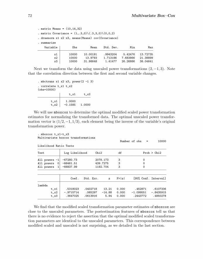
72 Multivariate Box–Cox

. matrix Means = (10,14,32)

. matrix Covariance = (1,.3,0)\(.3,3,0)\(0,0,2)

. drawnorm x1 x2 x3, means(Means) cov(Covariance)

. summarize

Variable Obs Mean Std. Dev. Min Max

x1 10000 10.00191 .9943204 5.42476 13.72735x2 10000 13.9793 1.713186 7.683866 21.38899x3 10000 31.98648 1.41477 26.26886 38.04641

Next we transform the data using unscaled power transformations (2,−1, 3). Notethat the correlation direction between the first and second variable changes.

. mbctrans x1 x2 x3, power(2 -1 3)

. correlate t_x1 t_x2(obs=10000)

t_x1 t_x2

t_x1 1.0000t_x2 -0.1585 1.0000

We will use mboxcox to determine the optimal modified scaled power transformationestimates for normalizing the transformed data. The optimal unscaled power transfor-mation vector is (1/2,−1, 1/3), each element being the inverse of the variable’s originaltransformation power.

. mboxcox t_x1-t_x3Multivariate boxcox transformations

Number of obs = 10000

Likelihood Ratio Tests

Test Log Likelihood Chi2 df Prob > Chi2

All powers -1 -67280.73 2078.173 3 0All powers 0 -66461.51 439.7275 3 0All powers 1 -66837.99 1192.704 3 0

Coef. Std. Err. z P>|z| [95% Conf. Interval]

lambdat_x1 .5318023 .0402718 13.21 0.000 .452871 .6107336t_x2 -.9715714 .065297 -14.88 0.000 -1.099551 -.8435915t_x3 .3647025 .0613916 5.94 0.000 .2443772 .4850278

We find that the modified scaled transformation parameter estimates of mboxcox areclose to the unscaled parameters. The postestimation features of mboxcox tell us thatthere is no evidence to reject the assertion that the optimal modified scaled transforma-tion parameters are identical to the unscaled parameters. This correspondence betweenmodified scaled and unscaled is not surprising, as we detailed in the last section.

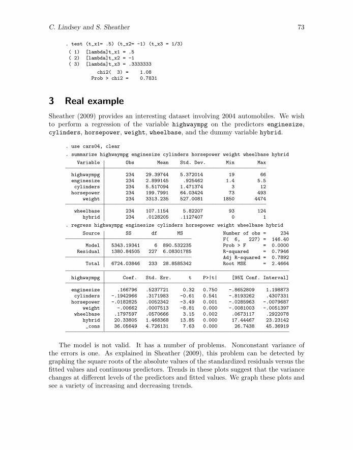
C. Lindsey and S. Sheather 73

. test (t_x1= .5) (t_x2= -1) (t_x3 = 1/3)

( 1) [lambda]t_x1 = .5( 2) [lambda]t_x2 = -1( 3) [lambda]t_x3 = .3333333

chi2( 3) = 1.08Prob > chi2 = 0.7831

3 Real example

Sheather (2009) provides an interesting dataset involving 2004 automobiles. We wishto perform a regression of the variable highwaympg on the predictors enginesize,cylinders, horsepower, weight, wheelbase, and the dummy variable hybrid.

. use cars04, clear

. summarize highwaympg enginesize cylinders horsepower weight wheelbase hybrid

Variable Obs Mean Std. Dev. Min Max

highwaympg 234 29.39744 5.372014 19 66enginesize 234 2.899145 .925462 1.4 5.5cylinders 234 5.517094 1.471374 3 12

horsepower 234 199.7991 64.03424 73 493weight 234 3313.235 527.0081 1850 4474

wheelbase 234 107.1154 5.82207 93 124hybrid 234 .0128205 .1127407 0 1

. regress highwaympg enginesize cylinders horsepower weight wheelbase hybrid

Source SS df MS Number of obs = 234F( 6, 227) = 146.40

Model 5343.19341 6 890.532235 Prob > F = 0.0000Residual 1380.84505 227 6.08301785 R-squared = 0.7946

Adj R-squared = 0.7892Total 6724.03846 233 28.8585342 Root MSE = 2.4664

highwaympg Coef. Std. Err. t P>|t| [95% Conf. Interval]

enginesize .166796 .5237721 0.32 0.750 -.8652809 1.198873cylinders -.1942966 .3171983 -0.61 0.541 -.8193262 .4307331

horsepower -.0182825 .0052342 -3.49 0.001 -.0285963 -.0079687weight -.00662 .0007513 -8.81 0.000 -.0081003 -.0051397

wheelbase .1797597 .0570666 3.15 0.002 .0673117 .2922078hybrid 20.33805 1.468368 13.85 0.000 17.44467 23.23142_cons 36.05649 4.726131 7.63 0.000 26.7438 45.36919

The model is not valid. It has a number of problems. Nonconstant variance ofthe errors is one. As explained in Sheather (2009), this problem can be detected bygraphing the square roots of the absolute values of the standardized residuals versus thefitted values and continuous predictors. Trends in these plots suggest that the variancechanges at different levels of the predictors and fitted values. We graph these plots andsee a variety of increasing and decreasing trends.

74 Multivariate Box–Cox

. predict rstd, rstandard

. predict fit, xb

. generate nsrstd = sqrt(abs(rstd))

. local i = 1

. foreach var of varlist fit enginesize cylinders horsepower weight wheelbase {2. twoway scatter nsrstd `var´ || lfit nsrstd `var´,

> ytitle("|Std. Residuals|^.5") legend(off)> ysize(5) xsize(5) name(gg`i´) nodraw

3. local i = `i´ + 14. }

. graph combine gg1 gg2 gg3 gg4 gg5 gg6, rows(2) ysize(10) xsize(15)

0.5

11.5

22.5

|Std

. R

esid

uals

|^.5

20 30 40 50 60Linear prediction

0.5

11.5

22.5

|Std

. R

esid

uals

|^.5

1 2 3 4 5 6EngineSize

0.5

11.5

22.5

|Std

. R

esid

uals

|^.5

2 4 6 8 10 12Cylinders

0.5

11.5

22.5

|Std

. R

esid

uals

|^.5

100 200 300 400 500Horsepower

0.5

11.5

22.5

|Std

. R

esid

uals

|^.5

2000 2500 3000 3500 4000 4500Weight

0.5

11.5

22.5

|Std

. R

esid

uals

|^.5

90 100 110 120 130WheelBase

Figure 1.√

|Standard residuals | versus predictors and fitted values.

Data transformation would be a strategy to solve the nonconstant variance problem. Assuggested in Weisberg (2005, 156), we should first examine linear relationships amongthe predictors. If they are approximately linearly related, we can use the fitted valuesto find a suitable transformation for the response, perhaps through an inverse responseplot (Sheather 2009). A matrix plot of the response and predictors shows that we willnot be able to do that. Many appear to share a monotonic relationship, but it is notlinear.

C. Lindsey and S. Sheather 75

HighwayMPG

EngineSize

Cylinders

Horsepower

Weight

WheelBase

20

40

60

20 40 60

2

4

6

2 4 6

5

10

15

5 10 15

0

500

0 500

2000

3000

4000

5000

2000 3000 4000 5000

90

100

110

120

90 100 110 120

Figure 2. Matrix plot original response and predictors.

20

30

40

50

60

70

Hig

hw

ayM

PG

12

34

56

En

gin

eS

ize

24

68

10

12

Cylin

de

rs

10

02

00

30

04

00

50

0H

ors

ep

ow

er

2,0

00

2,5

00

3,0

00

3,5

00

4,0

00

4,5

00

We

igh

t

90

10

01

10

12

01

30

Wh

ee

lBa

se

Figure 3. Box plots original response and predictors.

In addition, a look at the box plots reveals that several of the predictors and theresponse are skewed. The data are not consistent with a multivariate normal distribu-tion. If the predictors and response were multivariate normal conditioned on the valueof hybrid, then it would follow that the errors of the regression would have constantvariance. The conditional variance of multivariate normal variables is always constantwith regard to the values of the conditioning variables.

There are actually only three observations of hybrid that are nonzero. Data anal-ysis not shown here supports the contention that hybrid only significantly affects the

76 Multivariate Box–Cox

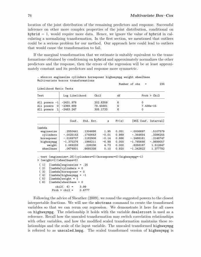
location of the joint distribution of the remaining predictors and response. Successfulinference on other more complex properties of the joint distribution, conditional onhybrid = 1, would require more data. Hence, we ignore the value of hybrid in cal-culating a normalizing transformation. In the first section, we mentioned that outlierscould be a serious problem for our method. Our approach here could lead to outliersthat would cause the transformation to fail.

If the marginal transformation that we estimate is suitably equivalent to the trans-formations obtained by conditioning on hybrid and approximately normalizes the otherpredictors and the response, then the errors of the regression will be at least approxi-mately constant and its predictors and response more symmetric.

. mboxcox enginesize cylinders horsepower highwaympg weight wheelbaseMultivariate boxcox transformations

Number of obs = 234

Likelihood Ratio Tests

Test Log Likelihood Chi2 df Prob > Chi2

All powers -1 -2431.978 202.6359 6 0All powers 0 -2369.889 78.45681 6 7.438e-15All powers 1 -2483.247 305.1733 6 0

Coef. Std. Err. z P>|z| [95% Conf. Interval]

lambdaenginesize .2550441 .1304686 1.95 0.051 -.0006697 .5107579cylinders -.0025143 .1745643 -0.01 0.989 -.344654 .3396255

horsepower -.0169707 .1182906 -0.14 0.886 -.2488161 .2148747highwaympg -1.375276 .1966211 -6.99 0.000 -1.760646 -.9899057

weight 1.069233 .226236 4.73 0.000 .6258187 1.512647wheelbase .0674801 .6685338 0.10 0.920 -1.242822 1.377782

. test (enginesize=.25)(cylinders=0)(horsepower=0)(highwaympg=-1)> (weight=1)(wheelbase=0)

( 1) [lambda]enginesize = .25( 2) [lambda]cylinders = 0( 3) [lambda]horsepower = 0( 4) [lambda]highwaympg = -1( 5) [lambda]weight = 1( 6) [lambda]wheelbase = 0

chi2( 6) = 3.99Prob > chi2 = 0.6777

Following the advice of Sheather (2009), we round the suggested powers to the closestinterpretable fractions. We will use the mbctrans command to create the transformedvariables so that we can rerun our regression. We demonstrate it here for all caseson highwaympg. The relationship it holds with the variable dealercost is used as areference. Recall how the unscaled transformation may switch correlation relationshipswith other variables, and how the modified scaled transformation maintains these re-lationships and the scale of the input variable. The unscaled transformed highwaympg

is referred to as unscaled hmpg. The scaled transformed version of highwaympg is

C. Lindsey and S. Sheather 77

named scaled hmpg. The modified scaled transformed version of highwaympg is namedmod scaled hmpg.

. summarize highwaympg

Variable Obs Mean Std. Dev. Min Max

highwaympg 234 29.39744 5.372014 19 66

. correlate dealercost highwaympg(obs=234)

dealer~t highwa~g

dealercost 1.0000highwaympg -0.5625 1.0000

. mbctrans highwaympg,power(-1)

. rename t_highwaympg unscaled_hmpg

. summarize unscaled_hmpg

Variable Obs Mean Std. Dev. Min Max

unscaled_h~g 234 .0349275 .0052762 .0151515 .0526316

. correlate dealercost unscaled_hmpg(obs=234)

dealer~t unscal~g

dealercost 1.0000unscaled_h~g 0.6779 1.0000

. mbctrans highwaympg,power(-1) scale

. rename t_highwaympg scaled_hmpg

. summarize scaled_hmpg

Variable Obs Mean Std. Dev. Min Max

scaled_hmpg 234 .9650725 .0052762 .9473684 .9848485

. correlate dealercost scaled_hmpg(obs=234)

dealer~t scaled~g

dealercost 1.0000scaled_hmpg -0.6779 1.0000

. mbctrans highwaympg,power(-1) mscale

. rename t_highwaympg mod_scaled_hmpg

. summarize mod_scaled_hmpg

Variable Obs Mean Std. Dev. Min Max

mod_scaled~g 234 810.9419 4.433584 796.0653 827.5595

. correlate dealercost mod_scaled_hmpg(obs=234)

dealer~t mod_sc~g

dealercost 1.0000mod_scaled~g -0.6779 1.0000

78 Multivariate Box–Cox

Both the scaled and modified scaled transformation kept the same correlation rela-tionship between highwaympg and dealercost. The unscaled transformation did not.Additionally, the modified scaled transformation maintained a scale much closer to thatof the original than either of the other transformations. Now we will use mbctrans onall the variables.

. mbctrans enginesize cylinders horsepower highwaympg weight wheelbase,> power(.25 0 0 -1 1 0) mscale

The box plots for the transformed data show a definite improvement in marginal nor-mality.

79

08

00

81

08

20

83

0t_

hig

hw

aym

pg

12

34

5t_

en

gin

esiz

e

68

10

12

14

t_cylin

de

rs

80

09

00

1,0

00

1,1

00

1,2

00

t_h

ors

ep

ow

er

2,0

00

2,5

00

3,0

00

3,5

00

4,0

00

4,5

00

t_w

eig

ht

48

04

90

50

05

10

52

0t_

wh

ee

lba

se

Figure 4. Box plots transformed response and predictors.

A matrix plot of the predictors and response shows greatly improved linearity.

C. Lindsey and S. Sheather 79

t_highwaympg

t_enginesize

t_cylinders

t_horsepower

t_weight

t_wheelbase

800

810

820

830

800 810 820 830

0

5

0 5

5

10

15

5 10 15

800

1000

1200

800 1000 1200

2000

3000

4000

5000

2000 3000 4000 5000

480

500

520

480 500 520

Figure 5. Matrix plot transformed response and predictors.

Now we refit the model with the transformed variables.

. regress t_highwaympg t_enginesize t_cylinders t_horsepower t_weight> t_wheelbase hybrid

Source SS df MS Number of obs = 234F( 6, 227) = 135.72

Model 3581.57374 6 596.928957 Prob > F = 0.0000Residual 998.430492 227 4.39837221 R-squared = 0.7820

Adj R-squared = 0.7762Total 4580.00424 233 19.6566705 Root MSE = 2.0972

t_highwaympg Coef. Std. Err. t P>|t| [95% Conf. Interval]

t_enginesize -.406318 .4557007 -0.89 0.374 -1.304262 .4916264t_cylinders -.5353418 .2622172 -2.04 0.042 -1.052033 -.0186507

t_horsepower -.0280757 .0051522 -5.45 0.000 -.038228 -.0179234t_weight -.0042486 .0006911 -6.15 0.000 -.0056103 -.0028868

t_wheelbase .2456528 .0490344 5.01 0.000 .1490321 .3422736hybrid 6.552501 1.276605 5.13 0.000 4.03699 9.068012_cons 735.9331 23.74779 30.99 0.000 689.1388 782.7274

. predict trstd, rstandard

. predict tfit, xb

. generate tnsrstd = sqrt(abs(trstd))

. local i = 1

. foreach var of varlist tfit t_enginesize t_cylinders t_horsepower t_weight> t_wheelbase {

2. twoway scatter tnsrstd `var´ || lfit tnsrstd `var´,> ytitle("|Std. Residuals|^.5") legend(off) ysize(5) xsize(5) name(gg`i´)> nodraw

3. local i = `i´ + 14. }

. graph combine gg1 gg2 gg3 gg4 gg5 gg6, rows(2) ysize(10) xsize(15)

80 Multivariate Box–Cox

The nonconstant variance has been drastically improved. The use of mboxcox helpedimprove the fit of the model.

0.5

11.5

2|S

td. R

esid

uals

|^.5

800 810 820 830Linear prediction

0.5

11.5

2|S

td. R

esid

uals

|^.5

1 2 3 4 5t_enginesize

0.5

11.5

2|S

td. R

esid

uals

|^.5

6 8 10 12 14t_cylinders

0.5

11.5

2|S

td. R

esid

uals

|^.5

800 900 1000 1100 1200t_horsepower

0.5

11.5

2|S

td. R

esid

uals

|^.5

2000 2500 3000 3500 4000 4500t_weight

0.5

11.5

2|S

td. R

esid

uals

|^.5

480 490 500 510 520t_wheelbase

Figure 6.√

|Standard residuals | versus transformed predictors and fitted values.

4 Conclusion

We explored both the theory and practice of the multivariate Box–Cox transformation.Using both generated and real datasets, we have demonstrated the use of the multivari-ate Box–Cox transformation in achieving multivariate normality and creating linearrelationships among variables.

We fully defined the mboxcox command as a method for performing the multivariateBox–Cox transformation in Stata. We also introduced the mbctrans command anddefined it as a method for performing the power transformations suggested by mboxcox.Finally, we also demonstrated the process of obtaining transformation power parameterestimates from mboxcox and rounding them to theoretically appropriate values.

5 References

Box, G. E. P., and D. R. Cox. 1964. An analysis of transformations. Journal of theRoyal Statistical Society, Series B 26: 211–252.

Riani, M., and A. C. Atkinson. 2000. Robust diagnostic data analysis: Transformationsin regression. Technometrics 42: 384–394.

Sheather, S. J. 2009. A Modern Approach to Regression with R. New York: Springer.

Velilla, S. 1993. A note on the multivariate Box–Cox transformation to normality.Statistics and Probability Letters 17: 259–263.

C. Lindsey and S. Sheather 81

———. 1995. Diagnostics and robust estimation in multivariate data transformations.Journal of the American Statistical Association 90: 945–951.

Weisberg, S. 2005. Applied Linear Regression. 3rd ed. New York: Wiley.

About the authors

Charles Lindsey is a PhD candidate in statistics at Texas A & M University. His researchis currently focused on nonparametric methods for regression and classification. He currentlyworks as a graduate research assistant for the Institute of Science Technology and PublicPolicy within the Bush School of Government and Public Service. He is also an instructor ofa course on sample survey techniques in Texas A & M University’s Statistics Department. Inthe summer of 2007, he worked as an intern at StataCorp. Much of the groundwork for thisarticle was formulated there.

Simon Sheather is professor and head of the Department of Statistics at Texas A & M Univer-sity. Simon’s research interests are in the fields of flexible regression methods, and nonpara-metric and robust statistics. In 2001, Simon was named an honorary fellow of the AmericanStatistical Association. Simon is currently listed on http://www.ISIHighlyCited.com amongthe top one-half of one percent of all mathematical scientists, in terms of citations of hispublished work.