IET Power and Energy Series 39 Power Systems Electromagnetic Transients Simulation Neville Watson and Jos Arrillaga

Welcome message from author
This document is posted to help you gain knowledge. Please leave a comment to let me know what you think about it! Share it to your friends and learn new things together.
Transcript
IET Power and Energy Series 39
Power Systems Electromagnetic
Transients Simulation
Neville Watson and Jos Arrillaga


Contents
List of figures xiii
List of tables xxi
Preface xxiii
Acronyms and constants xxv
1 Definitions, objectives and background 11.1 Introduction 11.2 Classification of electromagnetic transients 31.3 Transient simulators 41.4 Digital simulation 5
1.4.1 State variable analysis 51.4.2 Method of difference equations 5
1.5 Historical perspective 61.6 Range of applications 91.7 References 9
2 Analysis of continuous and discrete systems 112.1 Introduction 112.2 Continuous systems 11
2.2.1 State variable formulations 132.2.1.1 Successive differentiation 132.2.1.2 Controller canonical form 142.2.1.3 Observer canonical form 162.2.1.4 Diagonal canonical form 182.2.1.5 Uniqueness of formulation 192.2.1.6 Example 20
2.2.2 Time domain solution of state equations 202.2.3 Digital simulation of continuous systems 22
2.2.3.1 Example 272.3 Discrete systems 30

vi Contents
2.4 Relationship of continuous and discrete domains 322.5 Summary 342.6 References 34
3 State variable analysis 353.1 Introduction 353.2 Choice of state variables 353.3 Formation of the state equations 37
3.3.1 The transform method 373.3.2 The graph method 40
3.4 Solution procedure 433.5 Transient converter simulation (TCS) 44
3.5.1 Per unit system 453.5.2 Network equations 463.5.3 Structure of TCS 493.5.4 Valve switchings 513.5.5 Effect of automatic time step adjustments 533.5.6 TCS converter control 55
3.6 Example 593.7 Summary 643.8 References 65
4 Numerical integrator substitution 674.1 Introduction 674.2 Discretisation of R, L, C elements 68
4.2.1 Resistance 684.2.2 Inductance 684.2.3 Capacitance 704.2.4 Components reduction 71
4.3 Dual Norton model of the transmission line 734.4 Network solution 76
4.4.1 Network solution with switches 794.4.2 Example: voltage step applied to RL load 80
4.5 Non-linear or time varying parameters 884.5.1 Current source representation 894.5.2 Compensation method 894.5.3 Piecewise linear method 91
4.6 Subsystems 924.7 Sparsity and optimal ordering 954.8 Numerical errors and instabilities 974.9 Summary 974.10 References 98
5 The root-matching method 995.1 Introduction 995.2 Exponential form of the difference equation 99

Contents vii
5.3 z-domain representation of difference equations 1025.4 Implementation in EMTP algorithm 1055.5 Family of exponential forms of the difference equation 112
5.5.1 Step response 1145.5.2 Steady-state response 1165.5.3 Frequency response 117
5.6 Example 1185.7 Summary 1205.8 References 121
6 Transmission lines and cables 1236.1 Introduction 1236.2 Bergeron’s model 124
6.2.1 Multiconductor transmission lines 1266.3 Frequency-dependent transmission lines 130
6.3.1 Frequency to time domain transformation 1326.3.2 Phase domain model 136
6.4 Overhead transmission line parameters 1376.4.1 Bundled subconductors 1406.4.2 Earth wires 142
6.5 Underground cable parameters 1426.6 Example 1466.7 Summary 1566.8 References 156
7 Transformers and rotating plant 1597.1 Introduction 1597.2 Basic transformer model 160
7.2.1 Numerical implementation 1617.2.2 Parameters derivation 1627.2.3 Modelling of non-linearities 164
7.3 Advanced transformer models 1657.3.1 Single-phase UMEC model 166
7.3.1.1 UMEC Norton equivalent 1697.3.2 UMEC implementation in PSCAD/EMTDC 1717.3.3 Three-limb three-phase UMEC 1727.3.4 Fast transient models 176
7.4 The synchronous machine 1767.4.1 Electromagnetic model 1777.4.2 Electromechanical model 183
7.4.2.1 Per unit system 1847.4.2.2 Multimass representation 184
7.4.3 Interfacing machine to network 1857.4.4 Types of rotating machine available 189
7.5 Summary 1907.6 References 191

viii Contents
8 Control and protection 1938.1 Introduction 1938.2 Transient analysis of control systems (TACS) 1948.3 Control modelling in PSCAD/EMTDC 195
8.3.1 Example 1988.4 Modelling of protective systems 205
8.4.1 Transducers 2058.4.2 Electromechanical relays 2088.4.3 Electronic relays 2098.4.4 Microprocessor-based relays 2098.4.5 Circuit breakers 2108.4.6 Surge arresters 211
8.5 Summary 2138.6 References 214
9 Power electronic systems 2179.1 Introduction 2179.2 Valve representation in EMTDC 2179.3 Placement and location of switching instants 2199.4 Spikes and numerical oscillations (chatter) 220
9.4.1 Interpolation and chatter removal 2229.5 HVDC converters 2309.6 Example of HVDC simulation 2339.7 FACTS devices 233
9.7.1 The static VAr compensator 2339.7.2 The static compensator (STATCOM) 241
9.8 State variable models 2439.8.1 EMTDC/TCS interface implementation 2449.8.2 Control system representation 248
9.9 Summary 2489.10 References 249
10 Frequency dependent network equivalents 25110.1 Introduction 25110.2 Position of FDNE 25210.3 Extent of system to be reduced 25210.4 Frequency range 25310.5 System frequency response 253
10.5.1 Frequency domain identification 25310.5.1.1 Time domain analysis 25510.5.1.2 Frequency domain analysis 257
10.5.2 Time domain identification 26210.6 Fitting of model parameters 262
10.6.1 RLC networks 26210.6.2 Rational function 263
10.6.2.1 Error and figure of merit 265
Contents ix
10.7 Model implementation 26610.8 Examples 26710.9 Summary 27510.10 References 275
11 Steady state applications 27711.1 Introduction 27711.2 Initialisation 27811.3 Harmonic assessment 27811.4 Phase-dependent impedance of non-linear device 27911.5 The time domain in an ancillary capacity 281
11.5.1 Iterative solution for time invariant non-linearcomponents 282
11.5.2 Iterative solution for general non-linear components 28411.5.3 Acceleration techniques 285
11.6 The time domain in the primary role 28611.6.1 Basic time domain algorithm 28611.6.2 Time step 28611.6.3 DC system representation 28711.6.4 AC system representation 287
11.7 Voltage sags 28811.7.1 Examples 290
11.8 Voltage fluctuations 29211.8.1 Modelling of flicker penetration 294
11.9 Voltage notching 29611.9.1 Example 297
11.10 Discussion 29711.11 References 300
12 Mixed time-frame simulation 30312.1 Introduction 30312.2 Description of the hybrid algorithm 304
12.2.1 Individual program modifications 30712.2.2 Data flow 307
12.3 TS/EMTDC interface 30712.3.1 Equivalent impedances 30812.3.2 Equivalent sources 31012.3.3 Phase and sequence data conversions 31012.3.4 Interface variables derivation 311
12.4 EMTDC to TS data transfer 31312.4.1 Data extraction from converter waveforms 313
12.5 Interaction protocol 31312.6 Interface location 31612.7 Test system and results 31712.8 Discussion 31912.9 References 319

x Contents
13 Transient simulation in real time 32113.1 Introduction 32113.2 Simulation with dedicated architectures 322
13.2.1 Hardware 32313.2.2 RTDS applications 325
13.3 Real-time implementation on standard computers 32713.3.1 Example of real-time test 329
13.4 Summary 33013.5 References 331
A Structure of the PSCAD/EMTDC program 333A.1 References 340
B System identification techniques 341B.1 s-domain identification (frequency domain) 341B.2 z-domain identification (frequency domain) 343B.3 z-domain identification (time domain) 345B.4 Prony analysis 346B.5 Recursive least-squares curve-fitting algorithm 348B.6 References 350
C Numerical integration 351C.1 Review of classical methods 351C.2 Truncation error of integration formulae 354C.3 Stability of integration methods 356C.4 References 357
D Test systems data 359D.1 CIGRE HVDC benchmark model 359D.2 Lower South Island (New Zealand) system 359D.3 Reference 365
E Developing difference equations 367E.1 Root-matching technique applied to a first order lag function 367E.2 Root-matching technique applied to a first order
differential pole function 368E.3 Difference equation by bilinear transformation
for RL series branch 369E.4 Difference equation by numerical integrator substitution
for RL series branch 369
Contents xi
F MATLAB code examples 373F.1 Voltage step on RL branch 373F.2 Diode fed RL branch 374F.3 General version of example F.2 376F.4 Frequency response of difference equations 384
G FORTRAN code for state variable analysis 389G.1 State variable analysis program 389
H FORTRAN code for EMT simulation 395H.1 DC source, switch and RL load 395H.2 General EMT program for d.c. source, switch and RL load 397H.3 AC source diode and RL load 400H.4 Simple lossless transmission line 402H.5 Bergeron transmission line 404H.6 Frequency-dependent transmission line 407H.7 Utility subroutines for transmission line programs 413
Index 417

List of figures
1.1 Time frame of various transient phenomena 21.2 Transient network analyser 42.1 Impulse response associated with s-plane pole locations 232.2 Step response of lead–lag function 292.3 Norton of a rational function in z-domain 312.4 Data sequence associated with z-plane pole locations 322.5 Relationship between the domains 333.1 Non-trivial dependent state variables 363.2 Capacitive loop 383.3 (a) Capacitor with no connection to ground, (b) small capacitor added
to give a connection to ground 393.4 K matrix partition 413.5 Row echelon form 413.6 Modified state variable equations 423.7 Flow chart for state variable analysis 433.8 Tee equivalent circuit 453.9 TCS branch types 473.10 TCS flow chart 503.11 Switching in state variable program 513.12 Interpolation of time upon valve current reversal 523.13 NETOMAC simulation responses 543.14 TCS simulation with 1 ms time step 553.15 Steady state responses from TCS 563.16 Transient simulation with TCS for a d.c. short-circuit at 0.5 s 573.17 Firing control mechanism based on the phase-locked oscillator 583.18 Synchronising error in firing pulse 583.19 Constant αorder(15◦) operation with a step change in the d.c.
current 603.20 RLC test circuit 603.21 State variable analysis with 50 μs step length 613.22 State variable analysis with 50 μs step length 623.23 State variable analysis with 50 μs step length and x check 62
xiv List of figures
3.24 State variable with 50 μs step length and step length optimisation 633.25 Both x check and step length optimisation 633.26 Error comparison 644.1 Resistor 684.2 Inductor 684.3 Norton equivalent of the inductor 694.4 Capacitor 704.5 Norton equivalent of the capacitor 714.6 Reduction of RL branch 734.7 Reduction of RLC branch 744.8 Propagation of a wave on a transmission line 744.9 Equivalent two-port network for a lossless line 764.10 Node 1 of an interconnected circuit 774.11 Example using conversion of voltage source to current source 784.12 Network solution with voltage sources 804.13 Network solution with switches 814.14 Block diagonal structure 814.15 Flow chart of EMT algorithm 824.16 Simple switched RL load 834.17 Equivalent circuit for simple switched RL load 834.18 Step response of an RL branch for step lengths of �t = τ/10 and
�t = τ 864.19 Step response of an RL branch for step lengths of �t = 5τ and
�t = 10τ 874.20 Piecewise linear inductor represented by current source 894.21 Pictorial view of simultaneous solution of two equations 914.22 Artificial negative damping 924.23 Piecewise linear inductor 924.24 Separation of two coupled subsystems by means of linearised
equivalent sources 934.25 Interfacing for HVDC link 944.26 Example of sparse network 965.1 Norton equivalent for RL branch 1065.2 Switching test system 1075.3 Step response of switching test system for �t = τ 1075.4 Step response of switching test system for �t = 5τ 1085.5 Step response of switching test system for �t = 10τ 1085.6 Resonance test system 1095.7 Comparison between exponential form and Dommel’s method to a
5 kHz excitation for resonance test system. �t = 25 μs 1095.8 Comparison between exponential form and Dommel’s method to a
5 kHz excitation for resonance test system. �t = 10 μs 1105.9 Comparison between exponential form and Dommel’s method to
10 kHz excitation for resonance test system 110
List of figures xv
5.10 Response of resonance test system to 10 kHz excitation, blow-up ofexponential form’s response 111
5.11 Diode test system 1115.12 Response to diode test system (a) Voltage (b) Current 1125.13 Input as function of time 1135.14 Control or electrical system as first order lag 1135.15 Comparison step response of switching test system for �t = τ 1145.16 Comparison step response of switching test system for �t = 5τ 1155.17 Comparison of step response of switching test system for
�t = 10τ 1155.18 Root-matching type (d) approximation to a step 1165.19 Comparison with a.c. excitation (5 kHz) (�t = τ ) 1165.20 Comparison with a.c. excitation (10 kHz) (�t = τ ) 1175.21 Frequency response for various simulation methods 1186.1 Decision tree for transmission line model selection 1246.2 Nominal PI section 1246.3 Equivalent two-port network for line with lumped losses 1256.4 Equivalent two-port network for half-line section 1256.5 Bergeron transmission line model 1266.6 Schematic of frequency-dependent line 1296.7 Thevenin equivalent for frequency-dependent transmission line 1326.8 Norton equivalent for frequency-dependent transmission line 1326.9 Magnitude and phase angle of propagation function 1346.10 Fitted propagation function 1356.11 Magnitude and phase angle of characteristic impedance 1376.12 Transmission line geometry 1386.13 Matrix elimination of subconductors 1416.14 Cable cross-section 1426.15 Step response of a lossless line terminated by its characteristic
impedance 1476.16 Step response of a lossless line with a loading of double characteristic
impedance 1486.17 Step response of a lossless line with a loading of half its characteristic
impedance 1496.18 Step response of Bergeron line model for characteristic impedance
termination 1496.19 Step response of Bergeron line model for a loading of half its
characteristic impedance 1506.20 Step response of Bergeron line model for a loading of double
characteristic impedance 1506.21 Comparison of attenuation (or propagation) constant 1516.22 Error in fitted attenuation constant 1516.23 Comparison of surge impedance 1526.24 Error in fitted surge impedance 152

xvi List of figures
6.25 Step response of frequency-dependent transmission line model(load = 100 �) 153
6.26 Step response of frequency-dependent transmission line model(load = 1000 �) 154
6.27 Step response of frequency-dependent transmission line model(load = 50 �) 154
7.1 Equivalent circuit of the two-winding transformer 1607.2 Equivalent circuit of the two-winding transformer, without the
magnetising branch 1617.3 Transformer example 1617.4 Transformer equivalent after discretisation 1637.5 Transformer test system 1637.6 Non-linear transformer 1647.7 Non-linear transformer model with in-rush 1657.8 Star–delta three-phase transformer 1657.9 UMEC single-phase transformer model 1667.10 Magnetic equivalent circuit for branch 1677.11 Incremental and actual permeance 1687.12 UMEC Norton equivalent 1707.13 UMEC implementation in PSCAD/EMTDC 1717.14 UMEC PSCAD/EMTDC three-limb three-phase transformer
model 1737.15 UMEC three-limb three-phase Norton equivalent for blue phase
(Y-g/Y-g) 1757.16 Cross-section of a salient pole machine 1777.17 Equivalent circuit for synchronous machine equations 1807.18 The a.c. machine equivalent circuit 1827.19 d-axis flux paths 1837.20 Multimass model 1847.21 Interfacing electrical machines 1867.22 Electrical machine solution procedure 1877.23 The a.c. machine system 1887.24 Block diagram synchronous machine model 1898.1 Interface between network and TACS solution 1948.2 Continuous system model function library (PSCAD/EMTDC) 196/78.3 First-order lag 1988.4 Simulation results for a time step of 5 μs 2018.5 Simulation results for a time step of 50 μs 2028.6 Simulation results for a time step of 500 μs 2028.7 Simple bipolar PWM inverter 2048.8 Simple bipolar PWM inverter with interpolated turn ON and OFF 2048.9 Detailed model of a current transformer 2068.10 Comparison of EMTP simulation (solid line) and laboratory data
(dotted line) with high secondary burden 2078.11 Detailed model of a capacitive voltage transformer 208

List of figures xvii
8.12 Diagram of relay model showing the combination of electrical,magnetic and mechanical parts 209
8.13 Main components of digital relay 2108.14 Voltage–time characteristic of a gap 2118.15 Voltage–time characteristic of silicon carbide arrestor 2128.16 Voltage–time characteristic of metal oxide arrestor 2138.17 Frequency-dependent model of metal oxide arrestor 2139.1 Equivalencing and reduction of a converter valve 2189.2 Current chopping 2219.3 Illustration of numerical chatter 2229.4 Numerical chatter in a diode-fed RL load
(RON = 10−10,
ROFF = 1010) 2239.5 Forced commutation benchmark system 2239.6 Interpolation for GTO turn-OFF (switching and integration in one
step) 2249.7 Interpolation for GTO turn-OFF (using instantaneous solution) 2249.8 Interpolating to point of switching 2269.9 Jumps in variables 2269.10 Double interpolation method (interpolating back to the switching
instant) 2279.11 Chatter removal by interpolation 2289.12 Combined zero-crossing and chatter removal by interpolation 2299.13 Interpolated/extrapolated source values due to chatter removal
algorithm 2309.14 (a) The six-pulse group converter, (b) thyristor and snubber
equivalent circuit 2319.15 Phase-vector phase-locked oscillator 2319.16 Firing control for the PSCAD/EMTDC valve group model 2329.17 Classic V –I converter control characteristic 2329.18 CIGRE benchmark model as entered into the PSCAD draft
software 2349.19 Controller for the PSCAD/EMTDC simulation of the CIGRE
benchmark model 2359.20 Response of the CIGRE model to five-cycle three-phase fault at the
inverter bus 2369.21 SVC circuit diagram 2379.22 Thyristor switch-OFF with variable time step 2389.23 Interfacing between the SVC model and the EMTDC program 2399.24 SVC controls 2409.25 Basic STATCOM circuit 2419.26 Basic STATCOM controller 2429.27 Pulse width modulation 2439.28 Division of a network 2449.29 The converter system to be divided 2459.30 The divided HVDC system 246
xviii List of figures
9.31 Timing synchronisation 2469.32 Control systems in EMTDC 24710.1 Curve-fitting options 25410.2 Current injection 25410.3 Voltage injection 25510.4 PSCAD/EMTDC schematic with current injection 25610.5 Voltage waveform from time domain simulation 25710.6 Typical frequency response of a system 25810.7 Reduction of admittance matrices 25910.8 Multifrequency admittance matrix 26010.9 Frequency response 26110.10 Two-port frequency dependent network equivalent (admittance
implementation) 26110.11 Three-phase frequency dependent network equivalent (impedance
implementation) 26210.12 Ladder circuit of Hingorani and Burbery 26310.13 Ladder circuit of Morched and Brandwajn 26410.14 Magnitude and phase response of a rational function 26810.15 Comparison of methods for the fitting of a rational function 26910.16 Error for various fitted methods 26910.17 Small passive network 27010.18 Magnitude and phase fit for the test system 27110.19 Comparison of full and a passive FDNE for an energisation
transient 27210.20 Active FDNE 27210.21 Comparison of active FDNE response 27310.22 Energisation 27310.23 Fault inception and removal 27410.24 Fault inception and removal with current chopping 27411.1 Norton equivalent circuit 28211.2 Description of the iterative algorithm 28311.3 Test system at the rectifier end of a d.c. link 28811.4 Frequency dependent network equivalent of the test system 28811.5 Impedance/frequency of the frequency dependent equivalent 28911.6 Voltage sag at a plant bus due to a three-phase fault 29011.7 Test circuit for transfer switch 29111.8 Transfer for a 30 per cent sag at 0.8 power factor with a 3325 kVA
load 29211.9 EAF system single line diagram 29311.10 EAF without compensation 29311.11 EAF with SVC compensation 29411.12 EAF with STATCOM compensation 29411.13 Test system for flicker penetration (the circles indicate busbars and
the squares transmission lines) 295
List of figures xix
11.14 Comparison of Pst indices resulting from a positive sequence currentinjection 296
11.15 Test system for the simulation of voltage notching 29811.16 Impedance/frequency spectrum at the 25 kV bus 29911.17 Simulated 25 kV system voltage with drive in operation 29911.18 Simulated waveform at the 4.16 kV bus (surge capacitor location) 30012.1 The hybrid concept 30412.2 Example of interfacing procedure 30512.3 Modified TS steering routine 30612.4 Hybrid interface 30812.5 Representative circuit 30812.6 Derivation of Thevenin equivalent circuit 30912.7 Comparison of total r.m.s. power, fundamental frequency power and
fundamental frequency positive sequence power 31412.8 Normal interaction protocol 31512.9 Interaction protocol around a disturbance 31512.10 Rectifier terminal d.c. voltage comparisons 31812.11 Real and reactive power across interface 31812.12 Machine variables – TSE (TS variables) 31913.1 Schematic of real-time digital simulator 32113.2 Prototype real-time digital simulator 32313.3 Basic RTDS rack 32413.4 RTDS relay set-up 32613.5 Phase distance relay results 32713.6 HVDC control system testing 32713.7 Typical output waveforms from an HVDC control study 32813.8 General structure of the DTNA system 32813.9 Test system 32913.10 Current and voltage waveforms following a single-phase
short-circuit 330A.1 The PSCAD/EMTDC Version 2 suite 333A.2 DRAFT program 334A.3 RUNTIME program 335A.4 RUNTIME program showing controls and metering available 335A.5 MULTIPLOT program 336A.6 Interaction in PSCAD/EMTDC Version 2 337A.7 PSCAD/EMTDC flow chart 338A.8 PSCAD Version 3 interface 339C.1 Numerical integration from the sampled data viewpoint 353D.1 CIGRE HVDC benchmark test system 359D.2 Frequency scan of the CIGRE rectifier a.c. system impedance 361D.3 Frequency scan of the CIGRE inverter a.c. system impedance 361D.4 Frequency scan of the CIGRE d.c. system impedance 362D.5 Lower South Island of New Zealand test system 363

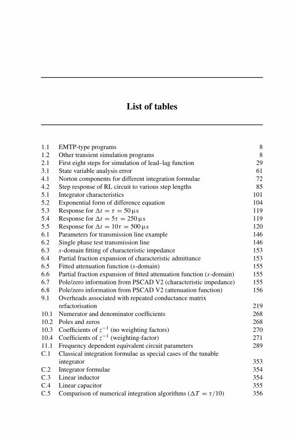
List of tables
1.1 EMTP-type programs 81.2 Other transient simulation programs 82.1 First eight steps for simulation of lead–lag function 293.1 State variable analysis error 614.1 Norton components for different integration formulae 724.2 Step response of RL circuit to various step lengths 855.1 Integrator characteristics 1015.2 Exponential form of difference equation 1045.3 Response for �t = τ = 50 μs 1195.4 Response for �t = 5τ = 250 μs 1195.5 Response for �t = 10τ = 500 μs 1206.1 Parameters for transmission line example 1466.2 Single phase test transmission line 1466.3 s-domain fitting of characteristic impedance 1536.4 Partial fraction expansion of characteristic admittance 1536.5 Fitted attenuation function (s-domain) 1556.6 Partial fraction expansion of fitted attenuation function (s-domain) 1556.7 Pole/zero information from PSCAD V2 (characteristic impedance) 1556.8 Pole/zero information from PSCAD V2 (attenuation function) 1569.1 Overheads associated with repeated conductance matrix
refactorisation 21910.1 Numerator and denominator coefficients 26810.2 Poles and zeros 26810.3 Coefficients of z−1 (no weighting factors) 27010.4 Coefficients of z−1 (weighting-factor) 27111.1 Frequency dependent equivalent circuit parameters 289C.1 Classical integration formulae as special cases of the tunable
integrator 353C.2 Integrator formulae 354C.3 Linear inductor 354C.4 Linear capacitor 355C.5 Comparison of numerical integration algorithms (�T = τ/10) 356

xxii List of tables
C.6 Comparison of numerical integration algorithms (�T = τ ) 356C.7 Stability region 357D.1 CIGRE model main parameters 360D.2 CIGRE model extra information 360D.3 Converter information for the Lower South Island test system 362D.4 Transmission line parameters for Lower South Island test system 362D.5 Conductor geometry for Lower South Island transmission lines
(in metres) 363D.6 Generator information for Lower South Island test system 363D.7 Transformer information for the Lower South Island test system 364D.8 System loads for Lower South Island test system (MW, MVar) 364D.9 Filters at the Tiwai-033 busbar 364E.1 Coefficients of a rational function in the z-domain for admittance 370E.2 Coefficients of a rational function in the z-domain for impedance 371E.3 Summary of difference equations 372
Preface
The analysis of electromagnetic transients has traditionally been discussed underthe umbrella of circuit theory, the main core course in the electrical engineeringcurriculum, and therefore the subject of very many textbooks. However, some of thespecial characteristics of power plant components, such as machine non-linearitiesand transmission line frequency dependence, have not been adequately covered inconventional circuit theory. Among the specialist books written to try and remedy thesituation are H. A. Peterson’s Transient performance in power systems (1951) andA. Greenwood’s Electric transients in power systems (1971). The former describedthe use of the transient network analyser to study the behaviour of linear and non-linear power networks. The latter described the fundamental concepts of the subjectand provided many examples of transient simulation based on the Laplace transform.
By the mid-1960s the digital computer began to determine the future patternof power system transients simulation. In 1976 the IEE published an importantmonograph, Computation of power system transients, based on pioneering computersimulation work carried out in the UK by engineers and mathematicians.
However, it was the IEEE classic paper by H. W. Dommel Digital computer solu-tion of electromagnetic transients in single and multiphase networks (1969), that setup the permanent basic framework for the simulation of power system electromag-netic transients in digital computers. Electromagnetic transient programs based onDommel’s algorithm, commonly known as the EMTP method, have now becomean essential part of the design of power apparatus and systems. They are also beinggradually introduced in the power curriculum of electrical engineering courses andplay an increasing role in their research and development programs.
Applications of the EMTP method are constantly reported in the IEE, IEEE andother international journals, as well as in the proceedings of many conferences, someof them specifically devoted to the subject, like the International Conference on PowerSystem Transients (IPST) and the International Conference on Digital Power SystemSimulators (ICDS). In 1997 the IEEE published a volume entitled Computer analysisof electric power system transients, which contained a comprehensive selection ofpapers considered as important contributions in this area. This was followed in 1998 bythe special publication TP-133-0 Modeling and analysis of system transients using

xxiv Preface
digital programs, a collection of published guidelines produced by various IEEEtaskforces.
Although there are well documented manuals to introduce the user to the variousexisting electromagnetic transients simulation packages, there is a need for a bookwith cohesive technical information to help students and professional engineers tounderstand the topic better and minimise the effort normally required to becomeeffective users of the EMT programs. Hopefully this book will fill that gap.
Basic knowledge of power system theory, matrix analysis and numerical tech-niques is presumed, but many references are given to help the readers to fill the gapsin their understanding of the relevant material.
The authors would like to acknowledge the considerable help received from manyexperts in the field, prior to and during the preparation of the book. In particularthey want to single out Hermann Dommel himself, who, during his study leave inCanterbury during 1983, directed our early attempts to contribute to the topic. Theyalso acknowledge the continuous help received from the Manitoba HVDC ResearchCentre, specially the former director Dennis Woodford, as well as Garth Irwin, nowboth with Electranix Corporation. Also, thanks are due to Ani Gole of the Universityof Manitoba for his help and for providing some of the material covered in thisbook. The providing of the paper by K. Strunz is also appreciated. The authors alsowish to thank the contributions made by a number of their colleagues, early on atUMIST (Manchester) and later at the University of Canterbury (New Zealand), suchas J. G. Campos Barros, H. Al Kashali, Chris Arnold, Pat Bodger, M. D. Heffernan,K. S. Turner, Mohammed Zavahir, Wade Enright, Glenn Anderson and Y.-P. Wang.Finally J. Arrillaga wishes to thank the Royal Society of New Zealand for the financialsupport received during the preparation of the book, in the form of the James CookSenior Research Fellowship.

Acronyms and constants
Acronyms
APSCOM Advances in Power System Control, Operation and ManagementATP Alternative Transient ProgramBPA Bonneville Power Administration (USA)CIGRE Conference Internationale des Grands Reseaux Electriques
(International Conference on Large High Voltage Electric Systems)DCG Development Coordination GroupEMT Electromagnetic TransientEMTP Electromagnetic Transients ProgramEMTDC1 Electromagnetic Transients Program for DCEPRI Electric Power Research Institute (USA)FACTS Flexible AC Transmission SystemsICDS International Conference on Digital Power System SimulatorsICHQP International Conference on Harmonics and Quality of PowerIEE The Institution of Electrical EngineersIEC International Electrotechnical CommissionIEEE Institute of Electrical and Electronics EngineersIREQ Laboratoire Simulation de Reseaux, Institut de Recherche
d’Hydro-QuebecNIS Numerical Integration SubstitutionMMF Magneto-Motive ForcePES Power Engineering SocietyPSCAD2 Power System Computer Aided DesignRTDS3 Real-Time Digital SimulatorSSTS Solid State Transfer SwitchTACS Transient Analysis of Control Systems
1 EMTDC is a registered trademark of the Manitoba Hydro2 PSCAD is a registered trademark of the Manitoba HVDC Research Centre3 RTDS is a registered trademark of the Manitoba HVDC Research Centre

xxvi Acronyms and constants
TCS Transient Converter Simulation (state variable analysis program)TRV Transient Recovery VoltageUIE Union International d’Electrothermie/International Union of Electroheat
Constants
ε0 permittivity of free space (8.85 × 10⁻¹² C2 N−1m−2 or F m−1)
μ0 permeability of free space (4π × 10−7 Wb A−1 m−1 or H m−1)
π 3.1415926535
c Speed of light (2.99793 × 10⁸ m s−1)

Chapter 1
Definitions, objectives and background
1.1 Introduction
The operation of an electrical power system involves continuous electromechanicaland electromagnetic distribution of energy among the system components. Duringnormal operation, under constant load and topology, these energy exchanges arenot modelled explicitly and the system behaviour can be represented by voltage andcurrent phasors in the frequency domain.
However, following switching events and system disturbances the energyexchanges subject the circuit components to higher stresses, resulting from exces-sive currents or voltage variations, the prediction of which is the main objective ofpower system transient simulation.
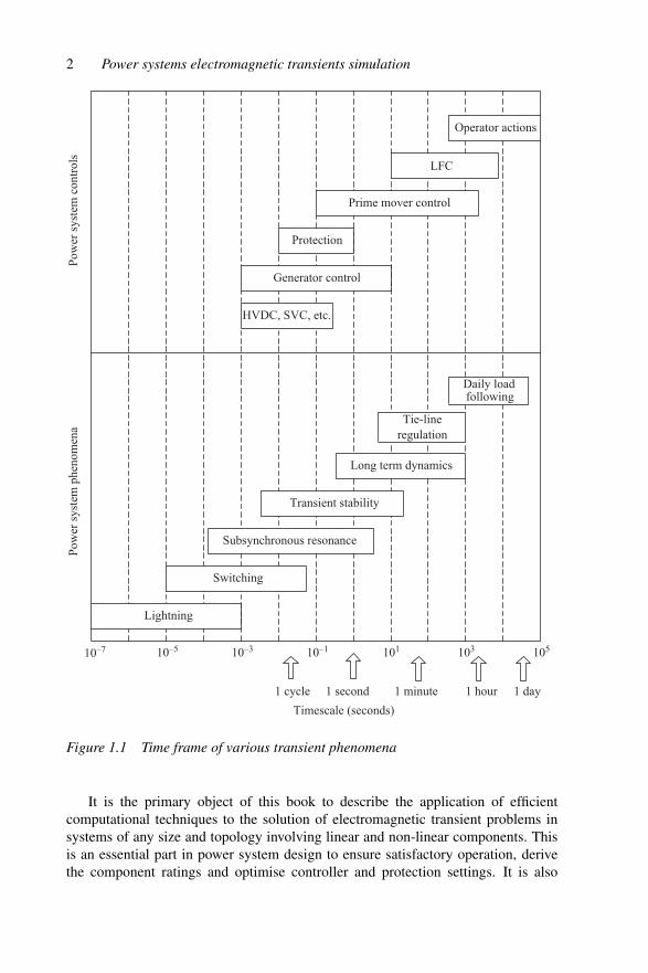
Figure 1.1 shows typical time frames for a full range of power system transients.The transients on the left of the figure involve predominantly interactions between themagnetic fields of inductances and the electric fields of capacitances in the system;they are referred to as electromagnetic transients. The transients on the right of thefigure are mainly affected by interactions between the mechanical energy stored in therotating machines and the electrical energy stored in the network; they are accordinglyreferred to as electromechanical transients. There is a grey area in the middle, namelythe transient stability region, where both effects play a part and may need adequaterepresentation.
In general the lightning stroke produces the highest voltage surges and thusdetermines the insulation levels. However at operating voltages of 400 kV andabove, system generated overvoltages, such as those caused by the energisation oftransmission lines, can often be the determining factor for insulation coordination.
From the analysis point of view the electromagnetic transients solution involvesa set of first order differential equations based on Kirchhoff’s laws, that describe thebehaviour of RLC circuits when excited by specified stimuli. This is a well documentedsubject in electrical engineering texts and it is therefore assumed that the readeris familiar with the terminology and concepts involved, as well as their physicalinterpretation.
2 Power systems electromagnetic transients simulation
10–7 10–5 10–3 10–1 101 103 105
Timescale (seconds)
Lightning
Switching
Subsynchronous resonance
Transient stability
Long term dynamics
Tie-lineregulation
Daily loadfollowing
HVDC, SVC, etc.
Generator control
Protection
Prime mover control
Operator actions
LFC
1 cycle 1 minute 1 hour 1 day1 second
Pow
er s
yste
m p
heno
men
aP
ower
sys
tem
con
trol
s
Figure 1.1 Time frame of various transient phenomena
It is the primary object of this book to describe the application of efficientcomputational techniques to the solution of electromagnetic transient problems insystems of any size and topology involving linear and non-linear components. Thisis an essential part in power system design to ensure satisfactory operation, derivethe component ratings and optimise controller and protection settings. It is also
Definitions, objectives and background 3
an important diagnostic tool to provide post-mortem information following systemincidents.
1.2 Classification of electromagnetic transients
Transient waveforms contain one or more oscillatory components and can thus becharacterised by the natural frequencies of these oscillations. However in the simula-tion process, the accurate determination of these oscillations is closely related to theequivalent circuits used to represent the system components. No component modelis appropriate for all types of transient analysis and must be tailored to the scope ofthe study.
From the modelling viewpoint, therefore, it is more appropriate to classify tran-sients by the time range of the study, which is itself related to the phenomena underinvestigation. The key issue in transient analysis is the selection of a model for eachcomponent that realistically represents the physical system over the time frame ofinterest.
Lightning, the fastest-acting disturbance, requires simulation in the region ofnano to micro-seconds. Of course in this time frame the variation of the power fre-quency voltage and current levels will be negligible and the electronic controllers willnot respond; on the other hand the stray capacitance and inductance of the systemcomponents will exercise the greatest influence in the response.
The time frame for switching events is in micro to milliseconds, as far as insu-lation coordination is concerned, although the simulation time can go into cycles,if system recovery from the disturbance is to be investigated. Thus, depending onthe information sought, switching phenomena may require simulations on differ-ent time frames with corresponding component models, i.e. either a fast transientmodel using stray parameters or one based on simpler equivalent circuits but includ-ing the dynamics of power electronic controllers. In each case, the simulation stepsize will need to be at least one tenth of the smallest time constant of the systemrepresented.
Power system components are of two types, i.e. those with essentially lumpedparameters, such as electrical machines and capacitor or reactor banks, and thosewith distributed parameters, including overhead lines and underground or submarinecables. Following a switching event these circuit elements are subjected to volt-ages and currents involving frequencies between 50 Hz and 100 kHz. Obviouslywithin such a vast range the values of the component parameters and of the earthpath will vary greatly with frequency. The simulation process therefore must becapable of reproducing adequately the frequency variations of both the lumped anddistributed parameters. The simulation must also represent such non-linearities asmagnetic saturation, surge diverter characteristics and circuit-breaker arcs. Of course,as important, if not more, as the method of solution is the availability of reliabledata and the variation of the system components with frequency, i.e. a fast tran-sient model including stray parameters followed by one based on simpler equivalentcircuits.

4 Power systems electromagnetic transients simulation
1.3 Transient simulators
Among the tools used in the past for the simulation of power system transients are theelectronic analogue computer, the transient network analyser (TNA) and the HVDCsimulator.
The electronic analogue computer basically solved ordinary differential equationsby means of several units designed to perform specific functions, such as adders,multipliers and integrators as well as signal generators and a multichannel cathoderay oscilloscope.
Greater versatility was achieved with the use of scaled down models and in par-ticular the TNA [1], shown in Figure 1.2, is capable of emulating the behaviourof the actual power system components using only low voltage and current levels.Early limitations included the use of lumped parameters to represent transmissionlines, unrealistic modelling of losses, ground mode of transmission lines and mag-netic non-linearities. However all these were largely overcome [2] and TNAs arestill in use for their advantage of operating in real time, thus allowing many runsto be performed quickly and statistical data obtained, by varying the instants ofswitching. The real-time nature of the TNA permits the connection of actual controlhardware and its performance validated, prior to their commissioning in the actualpower system. In particular, the TNA is ideal for testing the control hardware andsoftware associated with FACTS and HVDC transmission. However, due to theircost and maintenance requirements TNAs and HVDC models are being graduallydisplaced by real-time digital simulators, and a special chapter of the book is devotedto the latter.
Figure 1.2 Transient network analyser
Definitions, objectives and background 5
1.4 Digital simulation
Owing to the complexity of modern power systems, the simulators described abovecould only be relied upon to solve relatively simple problems. The advent of thedigital computer provided the stimulus to the development of more accurate andgeneral solutions. A very good description of the early digital methods can be foundin a previous monograph of this series [3].
While the electrical power system variables are continuous, digital simulationis by its nature discrete. The main task in digital simulation has therefore been thedevelopment of suitable methods for the solution of the differential and algebraicequations at discrete points.
The two broad classes of methods used in the digital simulation of the differentialequations representing continuous systems are numerical integration and differenceequations. Although the numerical integration method does not produce an explicitdifference equation to be simulated, each step of the solution can be characterised bya difference equation.
1.4.1 State variable analysis
State variable analysis is the most popular technique for the numerical integrationof differential equations [4]. This technique uses an indefinite numerical integrationof the system variables in conjunction with the differential equation (to obtain thederivatives of the states).
The differential equation is expressed in implicit form. Instead of rearranging itinto an explicit form, the state variable approach uses a predictor–corrector solution,such that the state equation predicts the state variable derivative and the trapezoidalrule corrects the estimates of the state variables.
The main advantages of this method are its simplicity and lack of overhead whenchanging step size, an important property in the presence of power electronic devicesto ensure that the steps are made to coincide with the switching instants. Thus thenumerical oscillations inherent in the numerical integration substitution techniquedo not occur; in fact the state variable method will fail to converge rather than giveerroneous answers. Moreover, non-linearities are easier to represent in state variableanalysis. The main disadvantages are greater solution time, extra code complexityand greater difficulty to model distributed parameters.
1.4.2 Method of difference equations
In the late 1960s H. W. Dommel of BPA (Bonneville Power Administration) developeda digital computer algorithm for the efficient analysis of power system electromag-netic transients [5]. The method, referred to as EMTP (ElectroMagnetic TransientsProgram), is based on the difference equations model and was developed around thetransmission system proposed by Bergeron [6].
Bergeron’s method uses linear relationships (characteristics) between the currentand the voltage, which are invariant from the point of view of an observer travelling

6 Power systems electromagnetic transients simulation
with the wave. However, the time intervals or discrete steps required by the digitalsolution generate truncation errors which can lead to numerical instability. The useof the trapezoidal rule to discretise the ordinary differential equations has improvedthe situation considerably in this respect.
Dommel’s EMTP method combines the method of characteristics and the trape-zoidal rule into a generalised algorithm which permits the accurate simulation oftransients in networks involving distributed as well as lumped parameters.
To reflect its main technical characteristics, Dommel’s method is often referredto by other names, the main one being numerical integration substitution. Other lesscommon names are the method of companion circuits (to emphasise the fact that thedifference equation can be viewed as a Norton equivalent, or companion, for eachelement in the circuit) and the nodal conductance approach (to emphasise the use ofthe nodal formulation).
There are alternative ways to obtain a discrete representation of a continuous func-tion to form a difference equation. For example the root-matching technique, whichdevelops difference equations such that the poles of its corresponding rational func-tion match those of the system being simulated, results in a very accurate and stabledifference equation. Complementary filtering is another technique of the numeri-cal integration substitution type to form difference equations that is inherently morestable and accurate. In the control area the widely used bilinear transform method(or Trustin’s method) is the same as numerical integration substitution developed byDommel in the power system area.
1.5 Historical perspective
The EMTP has become an industrial standard and many people have contributed toenhance its capability. With the rapid increase in size and complexity, documentation,maintenance and support became a problem and in 1982 the EMTP DevelopmentCoordination Group (DCG) was formed to address it.
In 1984 EPRI (Electric Power Research Institute) reached agreement with DCGto take charge of documentation, conduct EMTP validation tests and add a moreuser-friendly input processor. The development of new technical features remainedthe primary task of DCG. DCG/EPRI version 1.0 of EMTP was released in 1987 andversion 2.0 in 1989.
In order to make EMTP accessible to the worldwide community, the Alterna-tive Transient Program (ATP) was developed, with W.S. Meyer (of BPA) acting ascoordinator to provide support. Major contributions were made, among them TACS(Transient Analysis of Control Systems) by L. Dube in 1976, multi-phase untrans-posed transmission lines with constant parameters by C. P. Lee, a frequency-dependenttransmission line model and new line constants program by J. R. Marti, three-phasetransformer models by H. W. and I. I. Dommel, a synchronous machine model byV. Brandwajn, an underground cable model by L. Marti and synchronous machinedata conversion by H. W. Dommel.
Definitions, objectives and background 7
Inspired by the work of Dr. Dommel and motivated by the need to solve the prob-lems of frequently switching components (specifically HVDC converters) throughthe 1970s D. A. Woodford (of Manitoba Hydro) helped by A. Gole and R. Menziesdeveloped a new program still using the EMTP concept but designed around a.c.–d.c.converters. This program, called EMTDC (Electromagnetic Transients Program forDC), originally ran on mainframe computers.
With the development and universal availability of personal computers (PCs)EMTDC version 1 was released in the late 1980s. A data driven program can onlymodel components coded by the programmer, but, with the rapid technological devel-opments in power systems, it is impractical to anticipate all future needs. Therefore,to ensure that users are not limited to preprogrammed component models, EMTDCrequired the user to write two FORTRAN files, i.e. DSDYN (Digital SimulatorDYNamic subroutines) and DSOUT (Digital Simulator OUTput subroutines). Thesefiles are compiled and linked with the program object libraries to form the program.A BASIC program was used to plot the output waveforms from the files created.
The Manitoba HVDC Research Centre developed a comprehensive graphicaluser interface called PSCAD (Power System Computer Aided Design) to simplifyand speed up the simulation task. PSCAD/EMTDC version 2 was released in theearly 1990s for UNIX workstations. PSCAD comprised a number of programs thatcommunicated via TCP/IP sockets. DRAFT for example allowed the circuit to bedrawn graphically, and automatically generated the FORTRAN files needed to sim-ulate the system. Other modules were TLINE, CABLE, RUNTIME, UNIPLOT andMULTIPLOT.
Following the emergence of the Windows operating system on PCs as the domi-nant system, the Manitoba HVDC Research Centre rewrote PSCAD/EMTDC for thissystem. The Windows/PC based PSCAD/EMTDC version was released in 1998.
The other EMTP-type programs have also faced the same challenges with numer-ous graphical interfaces being developed, such as ATP_Draw for ATP. A more recenttrend has been to increase the functionality by allowing integration with other pro-grams. For instance, considering the variety of specialised toolboxes of MATLAB,it makes sense to allow the interface with MATLAB to benefit from the use of suchfacilities in the transient simulation program.
Data entry is always a time-consuming exercise, which the use of graphicalinterfaces and component libraries alleviates. In this respect the requirements of uni-versities and research organisations differ from those of electric power companies. Inthe latter case the trend has been towards the use of database systems rather than filesusing a vendor-specific format for power system analysis programs. This also helpsthe integration with SCADA information and datamining. An example of databaseusage is PowerFactory (produced by DIgSILENT). University research, on the otherhand, involves new systems for which no database exists and thus a graphical entrysuch as that provided by PSCAD is the ideal tool.
A selection, not exhaustive, of EMTP-type programs and their correspondingWebsites is shown in Table 1.1. Other transient simulation programs in current useare listed in Table 1.2. A good description of some of these programs is given inreference [7].

8 Power systems electromagnetic transients simulation
Table 1.1 EMTP-type programs
Program Organisation Website address
EPRI/DCG EMTP EPRI www.emtp96.com/ATP program www.emtp.org/MicroTran Microtran Power Systems
Analysis Corporationwww.microtran.com/
PSCAD/EMTDC Manitoba HVDC ResearchCentre
www.hvdc.ca/
NETOMAC Siemens www.ev.siemens.de/en/pages/NPLAN BCP Busarello + Cott +
Partner Inc.EMTAP EDSA www.edsa.com/PowerFactory DIgSILENT www.digsilent.de/Arene Anhelco www.anhelco.com/Hypersim IREQ (Real-time simulator) www.ireq.ca/RTDS RTDS Technologies rtds.caTransient Performance
Advisor (TPA)MPR (MATLAB based) www.mpr.com
Power System Toolbox Cherry Tree (MATLABbased)
www.eagle.ca/ cherry/
Table 1.2 Other transient simulation programs
Program Organisation Website address
ATOSEC5 University of Quebec atTrios Rivieres
cpee.uqtr.uquebec.ca/dctodc/ato5_1htm
Xtrans Delft University ofTechnology
eps.et.tudelft.nl
KREAN The Norwegian Universityof Science andTechnology
www.elkraft.ntnu.no/sie10aj/Krean1990.pdf
Power Systems MATHworks (MATLABbased)
www.mathworks.com/products/
Blockset TransEnergieTechnologies
www.transenergie-tech.com/en/
SABER Avant (formerly AnalogyInc.)
www.analogy.com/
SIMSEN Swiss Federal Institute ofTechnology
simsen.epfl.ch/

Definitions, objectives and background 9
1.6 Range of applications
Dommel’s introduction to his classical paper [5] started with the following statement:‘This paper describes a general solution method for finding the time response ofelectromagnetic transients in arbitrary single or multi-phase networks with lumpedand distributed parameters’.
The popularity of the EMTP method has surpassed all expectations, and threedecades later it is being applied in practically every problem requiring time domainsimulation. Typical examples of application are:
• Insulation coordination, i.e. overvoltage studies caused by fast transients with thepurpose of determining surge arrestor ratings and characteristics.
• Overvoltages due to switching surges caused by circuit breaker operation.• Transient performance of power systems under power electronic control.• Subsynchronous resonance and ferroresonance phenomena.
It must be emphasised, however, that the EMTP method was specifically devisedto provide simple and efficient electromagnetic transient solutions and not to solvesteady state problems. The EMTP method is therefore complementary to traditionalpower system load-flow, harmonic analysis and stability programs. However, it willbe shown in later chapters that electromagnetic transient simulation can also playan important part in the areas of harmonic power flow and multimachine transientstability.
1.7 References
1 PETERSON, H. A.: ‘An electric circuit transient analyser’, General ElectricReview, 1939, p. 394
2 BORGONOVO, G., CAZZANI, M., CLERICI, A., LUCCHINI, G. andVIDONI, G.: ‘Five years of experience with the new C.E.S.I. TNA’, IEEE CanadianCommunication and Power Conference, Montreal, 1974
3 BICKFORD, J. P., MULLINEUX, N. and REED J. R.: ‘Computation of power-systems transients’ (IEE Monograph Series 18, Peter Peregrinus Ltd., London,1976)
4 DeRUSSO, P. M., ROY, R. J., CLOSE, C. M. and DESROCHERS, A. A.: ‘Statevariables for engineers’ (John Wiley, New York, 2nd edition, 1998)
5 DOMMEL, H. W.: ‘Digital computer solution of electromagnetic transients insingle- and multi-phase networks’, IEEE Transactions on Power Apparatus andSystems, 1969, 88 (2), pp. 734–71
6 BERGERON, L.: ‘Du coup de Belier en hydraulique au coup de foudre en elec-tricite’ (Dunod, 1949). (English translation: ‘Water Hammer in hydraulics andwave surges in electricity’, ASME Committee, Wiley, New York, 1961.)
7 MOHAN, N., ROBBINS, W. P., UNDELAND, T. M., NILSSEN, R. and MO, O.:‘Simulation of power electronic and motion control systems – an overview’,Proceedings of the IEEE, 1994, 82 (8), pp. 1287–1302


Chapter 2
Analysis of continuous and discrete systems
2.1 Introduction
Linear algebra and circuit theory concepts are used in this chapter to describe theformulation of the state equations of linear dynamic systems. The Laplace transform,commonly used in the solution of simple circuits, is impractical in the context ofa large power system. Some practical alternatives discussed here are modal analy-sis, numerical integration of the differential equations and the use of differenceequations.
An electrical power system is basically a continuous system, with the exceptionsof a few auxiliary components, such as the digital controllers. Digital simulation, onthe other hand, is by nature a discrete time process and can only provide solutions forthe differential and algebraic equations at discrete points in time.
The discrete representation can always be expressed as a difference equation,where the output at a new time point is calculated from the output at previous timepoints and the inputs at the present and previous time points. Hence the digital repre-sentation can be synthesised, tuned, stabilised and analysed in a similar way as anydiscrete system.
Thus, as an introduction to the subject matter of the book, this chapter alsodiscusses, briefly, the subjects of digital simulation of continuous functions and theformulation of discrete systems.
2.2 Continuous systems
An nth order linear dynamic system is described by an nth order linear differentialequation which can be rewritten as n first-order linear differential equations, i.e.
x1(t) = a11x1(t) + a11x2(t) + · · · + a1nxn(t) + b11u1(t) + b12u2(t) + · · · + b1mum(t)
x2(t) = a21x1(t) + a22x2(t) + · · · + a2nxn(t) + b21u1(t) + b22u2(t) + · · · + b2mum(t)
...
xn(t) = an1x1(t) + an2x2(t) + · · · + annxn(t) + bn1u1(t) + bn2u2(t) + · · · + bnmum(t)
(2.1)
12 Power systems electromagnetic transients simulation
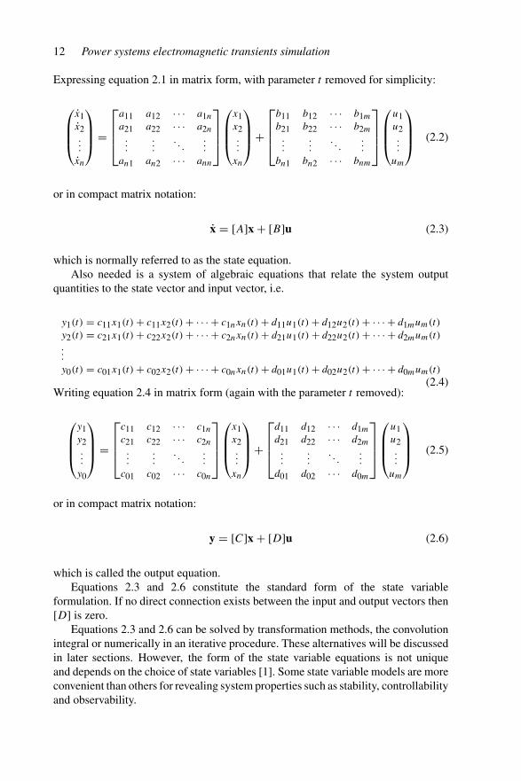
Expressing equation 2.1 in matrix form, with parameter t removed for simplicity:
⎛
⎜⎜⎝
x1x2...
xn
⎞
⎟⎟⎠ =
⎡
⎢⎢⎣
a11 a12 · · · a1n
a21 a22 · · · a2n...
.... . .
...
an1 an2 · · · ann
⎤
⎥⎥⎦
⎛
⎜⎜⎝
x1x2...
xn
⎞
⎟⎟⎠ +
⎡
⎢⎢⎣
b11 b12 · · · b1m
b21 b22 · · · b2m...
.... . .
...
bn1 bn2 · · · bnm
⎤
⎥⎥⎦
⎛
⎜⎜⎝
u1u2...
um
⎞
⎟⎟⎠ (2.2)
or in compact matrix notation:
x = [A]x + [B]u (2.3)
which is normally referred to as the state equation.Also needed is a system of algebraic equations that relate the system output
quantities to the state vector and input vector, i.e.
y1(t) = c11x1(t) + c11x2(t) + · · · + c1nxn(t) + d11u1(t) + d12u2(t) + · · · + d1mum(t)
y2(t) = c21x1(t) + c22x2(t) + · · · + c2nxn(t) + d21u1(t) + d22u2(t) + · · · + d2mum(t)
...
y0(t) = c01x1(t) + c02x2(t) + · · · + c0nxn(t) + d01u1(t) + d02u2(t) + · · · + d0mum(t)
(2.4)Writing equation 2.4 in matrix form (again with the parameter t removed):
⎛
⎜⎜⎝
y1y2...
y0
⎞
⎟⎟⎠ =
⎡
⎢⎢⎣
c11 c12 · · · c1n
c21 c22 · · · c2n...
.... . .
...
c01 c02 · · · c0n
⎤
⎥⎥⎦
⎛
⎜⎜⎝
x1x2...
xn
⎞
⎟⎟⎠ +
⎡
⎢⎢⎣
d11 d12 · · · d1m
d21 d22 · · · d2m...
.... . .
...
d01 d02 · · · d0m
⎤
⎥⎥⎦
⎛
⎜⎜⎝
u1u2...
um
⎞
⎟⎟⎠ (2.5)
or in compact matrix notation:
y = [C]x + [D]u (2.6)
which is called the output equation.Equations 2.3 and 2.6 constitute the standard form of the state variable
formulation. If no direct connection exists between the input and output vectors then[D] is zero.
Equations 2.3 and 2.6 can be solved by transformation methods, the convolutionintegral or numerically in an iterative procedure. These alternatives will be discussedin later sections. However, the form of the state variable equations is not uniqueand depends on the choice of state variables [1]. Some state variable models are moreconvenient than others for revealing system properties such as stability, controllabilityand observability.
Analysis of continuous and discrete systems 13
2.2.1 State variable formulations
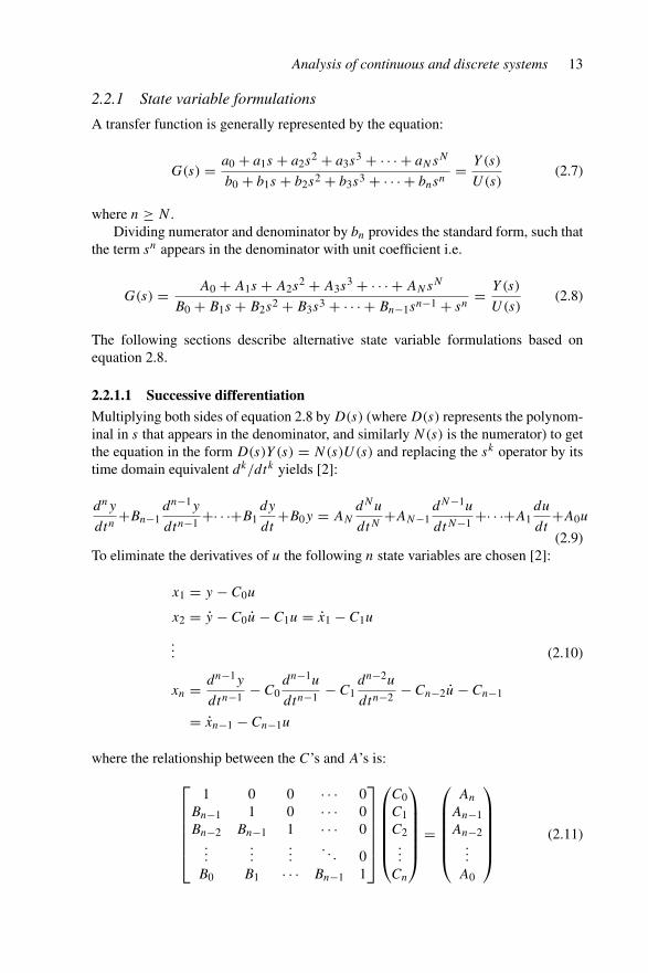
A transfer function is generally represented by the equation:
G(s) = a0 + a1s + a2s2 + a3s
3 + · · · + aNsN
b0 + b1s + b2s2 + b3s3 + · · · + bnsn= Y (s)
U(s)(2.7)
where n ≥ N .Dividing numerator and denominator by bn provides the standard form, such that
the term sn appears in the denominator with unit coefficient i.e.
G(s) = A0 + A1s + A2s2 + A3s
3 + · · · + ANsN
B0 + B1s + B2s2 + B3s3 + · · · + Bn−1sn−1 + sn= Y (s)
U(s)(2.8)
The following sections describe alternative state variable formulations based onequation 2.8.
2.2.1.1 Successive differentiation
Multiplying both sides of equation 2.8 by D(s) (where D(s) represents the polynom-inal in s that appears in the denominator, and similarly N(s) is the numerator) to getthe equation in the form D(s)Y (s) = N(s)U(s) and replacing the sk operator by itstime domain equivalent dk/dtk yields [2]:
dny
dtn+Bn−1
dn−1y
dtn−1+· · ·+B1
dy
dt+B0y = AN
dNu
dtN+AN−1
dN−1u
dtN−1+· · ·+A1
du
dt+A0u
(2.9)To eliminate the derivatives of u the following n state variables are chosen [2]:
x1 = y − C0u
x2 = y − C0u − C1u = x1 − C1u
... (2.10)
xn = dn−1y
dtn−1− C0
dn−1u
dtn−1− C1
dn−2u
dtn−2− Cn−2u − Cn−1
= xn−1 − Cn−1u
where the relationship between the C’s and A’s is:
⎡
⎢⎢⎢⎢⎢⎣
1 0 0 · · · 0Bn−1 1 0 · · · 0Bn−2 Bn−1 1 · · · 0
......
.... . . 0
B0 B1 · · · Bn−1 1
⎤
⎥⎥⎥⎥⎥⎦
⎛
⎜⎜⎜⎜⎜⎝
C0C1C2...
Cn
⎞
⎟⎟⎟⎟⎟⎠
=
⎛
⎜⎜⎜⎜⎜⎝
An
An−1An−2
...
A0
⎞
⎟⎟⎟⎟⎟⎠
(2.11)
14 Power systems electromagnetic transients simulation
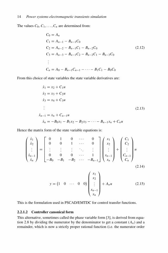
The values C0, C1, . . . , Cn are determined from:
C0 = An
C1 = An−1 − Bn−1C0
C2 = An−2 − Bn−1C1 − Bn−2C0 (2.12)
C3 = An−3 − Bn−1C2 − Bn−2C1 − Bn−3C0
...
Cn = A0 − Bn−1Cn−1 − · · · − B1C1 − B0C0
From this choice of state variables the state variable derivatives are:
x1 = x2 + C1u
x2 = x3 + C2u
x3 = x4 + C3u
... (2.13)
xn−1 = xn + Cn−1u
xn = −B0x1 − B1x2 − B2x3 − · · · − Bn−1xn + Cnu
Hence the matrix form of the state variable equations is:
⎛
⎜⎜⎜⎜⎜⎝
x1x2...
xn−1xn
⎞
⎟⎟⎟⎟⎟⎠
=
⎡
⎢⎢⎢⎢⎢⎣
0 1 0 · · · 00 0 1 · · · 0...
......
. . ....
0 0 0 · · · 1−B0 −B1 −B2 · · · −Bn−1
⎤
⎥⎥⎥⎥⎥⎦
⎛
⎜⎜⎜⎜⎜⎝
x1x2...
xn−1xn
⎞
⎟⎟⎟⎟⎟⎠
+
⎛
⎜⎜⎜⎜⎜⎝
C1C2...
Cn−1Cn
⎞
⎟⎟⎟⎟⎟⎠
u
(2.14)
y = (1 0 · · · 0 0
)
⎛
⎜⎜⎜⎜⎜⎝
x1x2...
xn−1xn
⎞
⎟⎟⎟⎟⎟⎠
+ Anu (2.15)
This is the formulation used in PSCAD/EMTDC for control transfer functions.
2.2.1.2 Controller canonical form
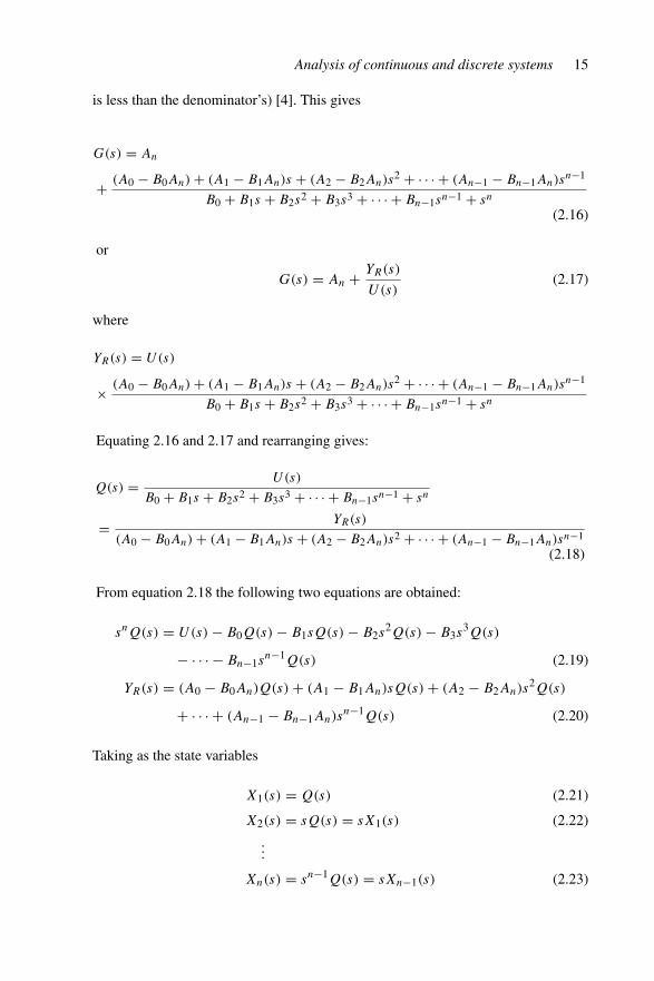
This alternative, sometimes called the phase variable form [3], is derived from equa-tion 2.8 by dividing the numerator by the denominator to get a constant (An) and aremainder, which is now a strictly proper rational function (i.e. the numerator order
Analysis of continuous and discrete systems 15
is less than the denominator’s) [4]. This gives
G(s) = An
+ (A0 − B0An) + (A1 − B1An)s + (A2 − B2An)s2 + · · · + (An−1 − Bn−1An)s
n−1
B0 + B1s + B2s2 + B3s3 + · · · + Bn−1sn−1 + sn
(2.16)
or
G(s) = An + YR(s)
U(s)(2.17)
where
YR(s) = U(s)
× (A0 − B0An) + (A1 − B1An)s + (A2 − B2An)s2 + · · · + (An−1 − Bn−1An)s
n−1
B0 + B1s + B2s2 + B3s3 + · · · + Bn−1sn−1 + sn
Equating 2.16 and 2.17 and rearranging gives:
Q(s) = U(s)
B0 + B1s + B2s2 + B3s3 + · · · + Bn−1sn−1 + sn
= YR(s)
(A0 − B0An) + (A1 − B1An)s + (A2 − B2An)s2 + · · · + (An−1 − Bn−1An)sn−1
(2.18)
From equation 2.18 the following two equations are obtained:
snQ(s) = U(s) − B0Q(s) − B1sQ(s) − B2s2Q(s) − B3s
3Q(s)
− · · · − Bn−1sn−1Q(s) (2.19)
YR(s) = (A0 − B0An)Q(s) + (A1 − B1An)sQ(s) + (A2 − B2An)s2Q(s)
+ · · · + (An−1 − Bn−1An)sn−1Q(s) (2.20)
Taking as the state variables
X1(s) = Q(s) (2.21)
X2(s) = sQ(s) = sX1(s) (2.22)
...
Xn(s) = sn−1Q(s) = sXn−1(s) (2.23)
16 Power systems electromagnetic transients simulation
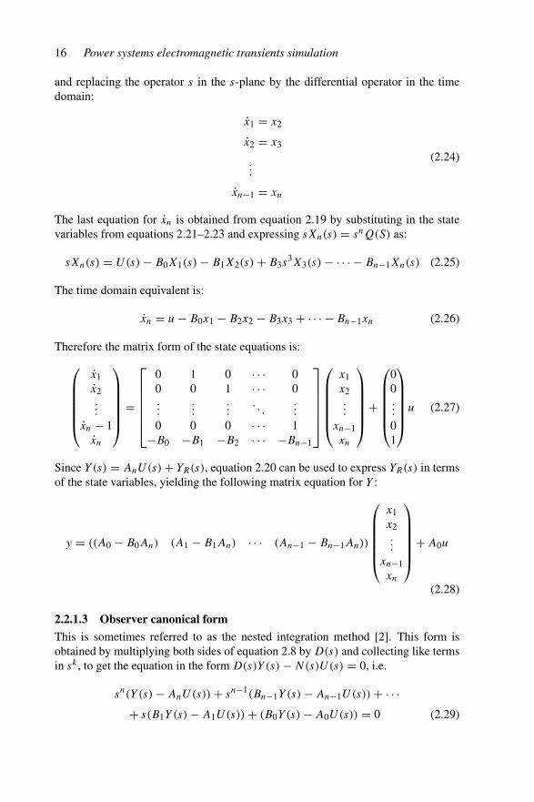
and replacing the operator s in the s-plane by the differential operator in the timedomain:
x1 = x2
x2 = x3
...
xn−1 = xn
(2.24)
The last equation for xn is obtained from equation 2.19 by substituting in the statevariables from equations 2.21–2.23 and expressing sXn(s) = snQ(S) as:
sXn(s) = U(s) − B0X1(s) − B1X2(s) + B3s3X3(s) − · · · − Bn−1Xn(s) (2.25)
The time domain equivalent is:
xn = u − B0x1 − B2x2 − B3x3 + · · · − Bn−1xn (2.26)
Therefore the matrix form of the state equations is:
⎛
⎜⎜⎜⎜⎜⎝
x1x2...
xn − 1xn
⎞
⎟⎟⎟⎟⎟⎠
=
⎡
⎢⎢⎢⎢⎢⎣
0 1 0 · · · 00 0 1 · · · 0...
......
. . ....
0 0 0 · · · 1−B0 −B1 −B2 · · · −Bn−1
⎤
⎥⎥⎥⎥⎥⎦
⎛
⎜⎜⎜⎜⎜⎝
x1x2...
xn−1xn
⎞
⎟⎟⎟⎟⎟⎠
+
⎛
⎜⎜⎜⎜⎜⎝
00...
01
⎞
⎟⎟⎟⎟⎟⎠
u (2.27)
Since Y (s) = AnU(s) + YR(s), equation 2.20 can be used to express YR(s) in termsof the state variables, yielding the following matrix equation for Y :
y = ((A0 − B0An) (A1 − B1An) · · · (An−1 − Bn−1An))
⎛
⎜⎜⎜⎜⎜⎝
x1x2...
xn−1xn
⎞
⎟⎟⎟⎟⎟⎠
+ A0u
(2.28)
2.2.1.3 Observer canonical form
This is sometimes referred to as the nested integration method [2]. This form isobtained by multiplying both sides of equation 2.8 by D(s) and collecting like termsin sk , to get the equation in the form D(s)Y (s) − N(s)U(s) = 0, i.e.
sn(Y (s) − AnU(s)) + sn−1(Bn−1Y (s) − An−1U(s)) + · · ·+ s(B1Y (s) − A1U(s)) + (B0Y (s) − A0U(s)) = 0 (2.29)
Analysis of continuous and discrete systems 17
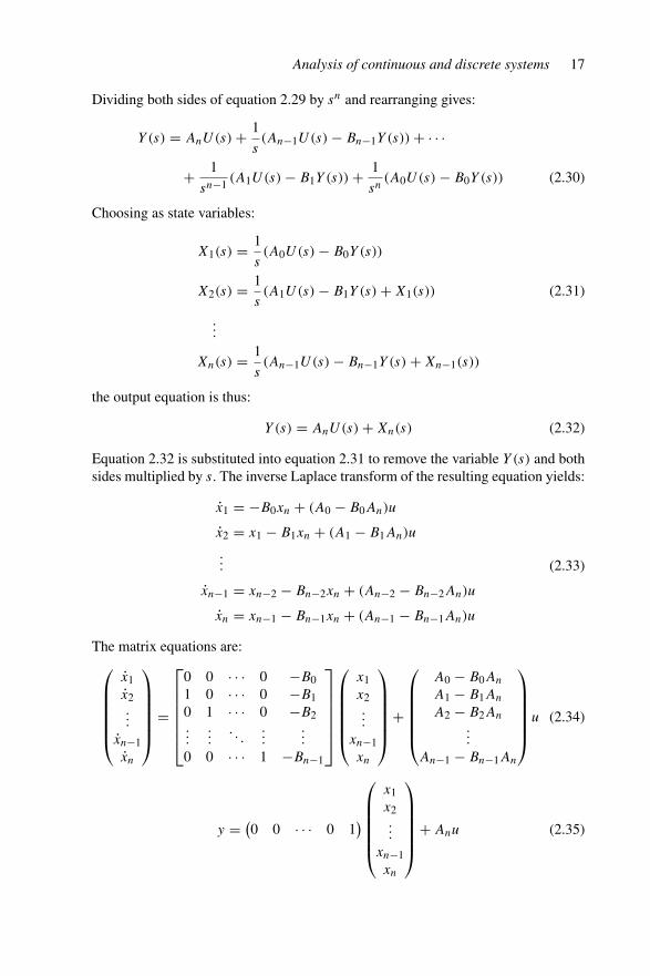
Dividing both sides of equation 2.29 by sn and rearranging gives:
Y (s) = AnU(s) + 1
s(An−1U(s) − Bn−1Y (s)) + · · ·
+ 1
sn−1(A1U(s) − B1Y (s)) + 1
sn(A0U(s) − B0Y (s)) (2.30)
Choosing as state variables:
X1(s) = 1
s(A0U(s) − B0Y (s))
X2(s) = 1
s(A1U(s) − B1Y (s) + X1(s)) (2.31)
...
Xn(s) = 1
s(An−1U(s) − Bn−1Y (s) + Xn−1(s))
the output equation is thus:
Y (s) = AnU(s) + Xn(s) (2.32)
Equation 2.32 is substituted into equation 2.31 to remove the variable Y (s) and bothsides multiplied by s. The inverse Laplace transform of the resulting equation yields:
x1 = −B0xn + (A0 − B0An)u
x2 = x1 − B1xn + (A1 − B1An)u
... (2.33)
xn−1 = xn−2 − Bn−2xn + (An−2 − Bn−2An)u
xn = xn−1 − Bn−1xn + (An−1 − Bn−1An)u
The matrix equations are:⎛
⎜⎜⎜⎜⎜⎝
x1x2...
xn−1xn
⎞
⎟⎟⎟⎟⎟⎠
=
⎡
⎢⎢⎢⎢⎢⎣
0 0 · · · 0 −B01 0 · · · 0 −B10 1 · · · 0 −B2...
.... . .
......
0 0 · · · 1 −Bn−1
⎤
⎥⎥⎥⎥⎥⎦
⎛
⎜⎜⎜⎜⎜⎝
x1x2...
xn−1xn
⎞
⎟⎟⎟⎟⎟⎠
+
⎛
⎜⎜⎜⎜⎜⎝
A0 − B0An
A1 − B1An
A2 − B2An
...
An−1 − Bn−1An
⎞
⎟⎟⎟⎟⎟⎠
u (2.34)
y = (0 0 · · · 0 1
)
⎛
⎜⎜⎜⎜⎜⎝
x1x2...
xn−1xn
⎞
⎟⎟⎟⎟⎟⎠
+ Anu (2.35)

18 Power systems electromagnetic transients simulation
2.2.1.4 Diagonal canonical form
The diagonal canonical or Jordan form is derived by rewriting equation 2.7 as:
G(s) = A0 + A1s + A2s2 + A3s
3 + · · · + ANsN
(s − λ1)(s − λ2)(s − λ3) · · · (s − λn)= Y (s)
U(s)(2.36)
where λk are the poles of the transfer function. By partial fraction expansion:
G(s) = r1
(s − λ1)+ r2
(s − λ2)+ r3
(s − λ3)+ · · · + rn
(s − λn)+ D (2.37)
or
G(s) = Y (s)
U(s)= r1
p1
U(s)+ r2
p2
U(s)+ r3
p3
U(s)+ · · · + rn
pn
U(s)+ D (2.38)
where
pi = U(s)
(s − λi)D =
{An, N = n
0, N < n(2.39)
which gives
Y (s) = r1p1 + r2p2 + r3p3 + · · · + rnpn + DU(s) (2.40)
In the time domain equation 2.39 becomes:
pi = λipi + u (2.41)
and equation 2.40:
y =n∑
1
ripi + Du (2.42)
for i = 1, 2, . . . , n; or, in compact matrix notation,
p = [λ]p + [β]u (2.43)
y = [C]p + Du (2.44)
where
[λ] =
⎡
⎢⎢⎢⎣
λ1 0 · · · 00 λ2 · · · 0...
.... . . 0
0 0 · · · λn
⎤
⎥⎥⎥⎦
, [β] =
⎡
⎢⎢⎢⎣
11...
1
⎤
⎥⎥⎥⎦
, [C] =
⎡
⎢⎢⎢⎣
r1r2...
rN
⎤
⎥⎥⎥⎦
and the λ terms in the Jordans’ form are the eigenvalues of the matrix [A].

Analysis of continuous and discrete systems 19
2.2.1.5 Uniqueness of formulation
The state variable realisation is not unique; for example another possible state variableform for equation 2.36 is:
⎛
⎜⎜⎜⎝
x1x2...
xn
⎞
⎟⎟⎟⎠
=
⎡
⎢⎢⎢⎢⎢⎣
−Bn−1 1 0 · · · 0−Bn−2 0 1 · · · 0
......
.... . .
...
−B1 0 0 · · · 1−B0 0 0 · · · 0
⎤
⎥⎥⎥⎥⎥⎦
⎛
⎜⎜⎜⎝
x1x2...
xD
⎞
⎟⎟⎟⎠
+
⎛
⎜⎜⎜⎜⎜⎝
An−1 − Bn−1An
An−2 − Bn−2An
...
A1 − B1An
A0 − B0An
⎞
⎟⎟⎟⎟⎟⎠
u (2.45)
However the transfer function is unique and is given by:
H(s) = [C](s[I ] − [A])−1[B] + [D] (2.46)
For low order systems this can be evaluated using:
(s[I ] − [A])−1 = adj(s[I ] − [A])|s[I ] − [A]| (2.47)
where [I ] is the identity matrix.In general a non-linear network will result in equations of the form:
x = [A]x + [B]u + [B1]u + ([B2]u + · · · )y = [C]x + [D]u + [D1]u + ([D2]u + · · · ) (2.48)
For linear RLC networks the derivative of the input can be removed by a simple changeof state variables, i.e.
x′ = x − [B1]u (2.49)
The state variable equations become:
x′ = [A]x′ + [B]u (2.50)
y = [C]x′ + [D]u (2.51)
However in general non-linear networks the time derivative of the forcing functionappears in the state and output equations and cannot be readily eliminated.
Generally the differential equations for a circuit are of the form:
[M]x = [A(0)]x + [B(0)]u + ([B(0)1]u) (2.52)
To obtain the normal form, both sides are multiplied by the inverse of [M]−1, i.e.
x = [M]−1[A(0)]x + [M]−1[B(0)]u +([M]−1[B(0)1]u
)
= [A]x + [B]u + ([B1]u) (2.53)

20 Power systems electromagnetic transients simulation
2.2.1.6 Example
Given the transfer function:
Y (s)
U(s)= s + 3
s2 + 3s + 2= 2
(s + 1)+ −1
(s + 2)
derive the alternative state variable representations described in sections2.2.1.1–2.2.1.4.Successive differentiation:
(x1x2
)=
[0 1
−2 −3
](x1x2
)+
(10
)u (2.54)
y = [1 0
](
x1x2
)(2.55)
Controllable canonical form:(
x1x2
)=
[0 1
−2 −3
](x1x2
)+
(01
)u (2.56)
y = [3 1
] (x1x2
)(2.57)
Observable canonical form:(
x1x2
)=
[0 −21 −3
](x1x2
)+
(31
)u (2.58)
y = [0 1
] (x1x2
)(2.59)
Diagonal canonical form:(
x1x2
)=
[−1 00 −2
](x1x2
)+
(11
)u (2.60)
y = [2 −1
] (x1x2
)(2.61)
Although all these formulations look different they represent the same dynamic sys-tem and their response is identical. It is left as an exercise to calculate H(s) =[C](s[I ] − [A])−1[B] + [D] to show they all represent the same transfer function.
2.2.2 Time domain solution of state equations
The Laplace transform of the state equation is:
sX(s) − X(0+) = [A]X(s) + [B]U(s) (2.62)
Therefore
X(s) = (s[I ] − [A])−1X(0+) + (s[I ] − [A])−1[B]U(s) (2.63)
where [I ] is the identity (or unit) matrix.
Analysis of continuous and discrete systems 21
Then taking the inverse Laplace transform will give the time response. Howeverthe use of the Laplace transform method is impractical to determine the transientresponse of large networks with arbitrary excitation.
The time domain solution of equation 2.63 can be expressed as:
x(t) = h(t)x(0+) +∫ t
0h(t − T )[B]u(T ) dT (2.64)
or, changing the lower limit from 0 to t0:
x(t) = e[A](t−t0)x(t0) +∫ t
t0
e[A](t−T )[B]u(T ) dT (2.65)
where h(t), the impulse response, is the inverse Laplace transform of the transitionmatrix, i.e. h(t) = L−1((sI − [A])−1).
The first part of equation 2.64 is the homogeneous solution due to the initialconditions. It is also referred to as the natural response or the zero-input response, ascalculated by setting the forcing function to zero (hence the homogeneous case). Thesecond term of equation 2.64 is the forced solution or zero-state response, which canalso be expressed as the convolution of the impulse response with the source. Thusequation 2.64 becomes:
x(t) = h(t)x(0+) + h(t) ⊗ [B]u(t) (2.66)
Only simple analytic solutions can be obtained by transform methods, as this requirestaking the inverse Laplace transform of the impulse response transfer function matrix,which is difficult to perform. The same is true for the method of variation of parameterswhere integrating factors are applied.
The time convolution can be performed by numerical calculation. Thus by applica-tion of an integration rule a difference equation can be derived. The simplest approachis the use of an explicit integration method (such that the value at t + �t is onlydependent on t values), however it suffers from the weaknesses of explicit methods.Applying the forward Euler method will give the following difference equation forthe solution [5]:
x(t + �t) = e[A]�tx(t) + [A]−1(e[A]�t − I )[B]u(t) (2.67)
As can be seen the difference equation involves the transition matrix, which must beevaluated via its series expansion, i.e.
e[A]�t = I + [A]�t + [A]2�t2
2! + [A]3�t3
3! + · · · (2.68)
However this is not always straightforward and, even when convergence is possible,it may be very slow. Moreover, alternative terms of the series have opposite signs andthese terms may have extremely high values.
The calculation of equation 2.68 may be aided by modal analysis. This is achievedby determining the eigenvalues and eigenvectors, hence the transformation matrix [T ],which will diagonalise the transition matrix i.e.
z = [T ]−1[A][T ]z + [T ]−1[B]u = [S]z + [T ]−1[B]u (2.69)

22 Power systems electromagnetic transients simulation
where
z = [T ]−1x
[S] =
⎡
⎢⎢⎢⎢⎢⎣
λ1 0 · · · 0 00 λ2 · · · 0 0...
.... . .
......
0 0 · · · λn−1 00 0 · · · 0 λn
⎤
⎥⎥⎥⎥⎥⎦
and λ1, . . . , λn are the eigenvalues of the matrix.The eigenvalues provide information on time constants, resonant frequencies and
stability of a system. The time constants of the system (1/�e(λmin)) indicate thelength of time needed to reach steady state and the maximum time step that can beused. The ratio of the largest to smallest eigenvalues (λmax/λmin) gives an indicationof the stiffness of the system, a large ratio indicating that the system is mathematicallystiff.
An alternative method of solving equation 2.65 is the use of numerical integration.In this case, state variable analysis uses an iterative procedure (predictor–correctorformulation) to solve for each time period. An implicit integration method, such asthe trapezoidal rule, is used to calculate the state variables at time t , however thisrequires the value of the state variable derivatives at time t . The previous time stepvalues can be used as an initial guess and once an estimate of the state variableshas been obtained using the trapezoidal rule, the state equation is used to update theestimate of the state variable derivatives.
No matter how the differential equations are arranged and manipulated into differ-ent forms, the end result is only a function of whether a numerical integration formulais substituted in (discussed in section 2.2.3) or an iterative solution procedure adopted.
2.2.3 Digital simulation of continuous systems
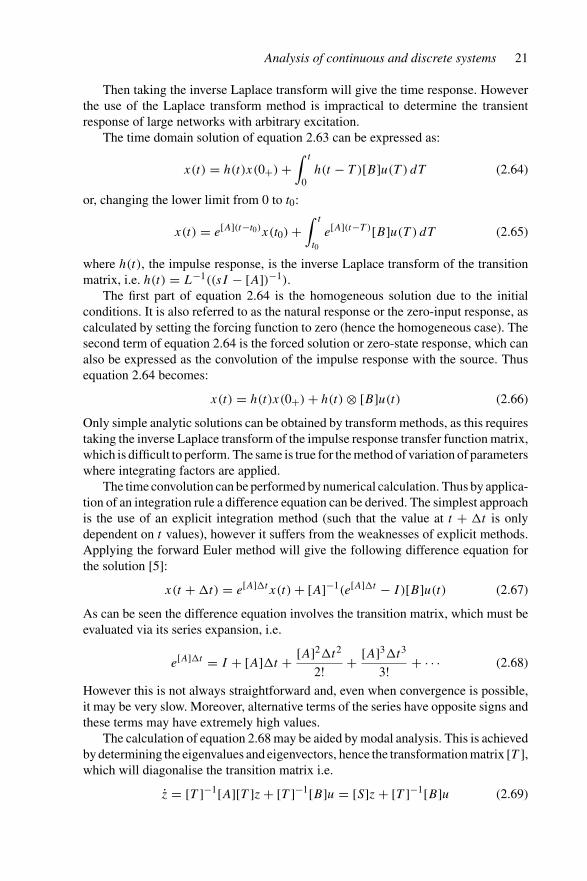
As explained in the introduction, due to the discrete nature of the digital process,a difference equation must be developed to allow the digital simulation of a continuoussystem. Also the latter must be stable to be able to perform digital simulation, whichimplies that all the s-plane poles are in the left-hand half-plane, as illustrated inFigure 2.1.
However, the stability of the continuous system does not necessarily ensure that thesimulation equations are stable. The equivalent of the s-plane for continuous signals isthe z-plane for discrete signals. In the latter case, for stability the poles must lie insidethe unit circle, as shown in Figure 2.4 on page 32. Thus the difference equations mustbe transformed to the z-plane to assess their stability. Time delay effects in the waydata is manipulated must be incorporated and the resulting z-domain representationused to determine the stability of the simulation equations.
Analysis of continuous and discrete systems 23
Imaginaryaxis
Real axis
Out
put
Out
put
Out
put
Out
put
Out
put
Time
Time
Time
Time
Time
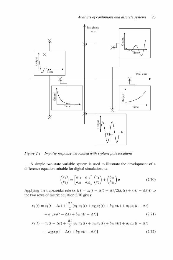
Figure 2.1 Impulse response associated with s-plane pole locations
A simple two-state variable system is used to illustrate the development of adifference equation suitable for digital simulation, i.e.
(x1x2
)=
[a11 a12a21 a22
](x1x2
)+
(b11b21
)u (2.70)
Applying the trapezoidal rule (xi(t) = xi(t − �t) + �t/2(xi(t) + xi (t − �t))) tothe two rows of matrix equation 2.70 gives:
x1(t) = x1(t − �t) + �t
2[a11x1(t) + a12x2(t) + b11u(t) + a11x1(t − �t)
+ a12x2(t − �t) + b11u(t − �t)] (2.71)
x2(t) = x2(t − �t) + �t
2[a21x1(t) + a22x2(t) + b21u(t) + a21x1(t − �t)
+ a22x2(t − �t) + b21u(t − �t)] (2.72)
24 Power systems electromagnetic transients simulation
or in matrix form:⎡
⎢⎣
1 − �t
2a11 −�t
2a12
−�t
2a21 1 − �t
2a22
⎤
⎥⎦
(x1(t)
x2(t)
)
=⎡
⎢⎣
1 + �t
2a11
�t
2a12
�t
2a21 1 + �t
2a22
⎤
⎥⎦
(x1(t − �t)
x2(t − �t)
)
+⎛
⎜⎝
�t
2b11
�t
2b21
⎞
⎟⎠ (u(t) + u(t − �t)) (2.73)
Hence the set of difference equations to be solved at each time point is:
(x1(t)
x2(t)
)
=⎡
⎢⎣
1 − �t
2a11 −�t
2a12
−�t
2a21 1 − �t
2a22
⎤
⎥⎦
−1 ⎡
⎢⎣
1 + �t
2a11
�t
2a12
�t
2a21 1 + �t
2a22
⎤
⎥⎦
(x1(t − �t)
x2(t − �t)
)
+⎡
⎢⎣
1 − �t
2a11 −�t
2a12
−�t
2a21 1 − �t
2a22
⎤
⎥⎦
−1 ⎛
⎜⎝
�t
2b11
�t
2b21
⎞
⎟⎠ (u(t) + u(t − �t)) (2.74)
This can be generalised for any state variable formulation by substituting the stateequation (x = [A]x + [B]u) into the trapezoidal equation i.e.
x(t) = x(t − �t) + �t
2(x(t) + x(t − �t))
= x(t − �t) + �t
2([A] x(t) + [B] u(t) + [A] x(t − �t) + [B] u(t − �t))
(2.75)
Collecting terms in x(t), x(t − �t), u(t) and u(t − �t) gives:(
[I ] − �t
2[A]
)x(t) =
([I ] + �t
2[A]
)x(t − �t) + �t
2[B] (u(t) + u(t − �t))
(2.76)Rearranging equation 2.76 to give x(t) in terms of previous time point values andpresent input yields:
x(t) =[[I ] − �t
2[A]
]−1 [[I ] + �t
2[A]
]x(t − �t)
+[[I ] − �t
2[A]
]−1�t
2[B] (u(t) + u(t − �t)) (2.77)
The structure of ([I ] − �t/2[A]) depends on the formulation, for example with thesuccessive differentiation approach (used in PSCAD/EMTDC for transfer function

Analysis of continuous and discrete systems 25
representation) it becomes:⎡
⎢⎢⎢⎢⎢⎢⎢⎢⎢⎢⎢⎢⎢⎣
1 −�t
20 · · · 0 0
0 1 −�t
2
. . ....
...
0 0 1. . . 0 0
......
.... . . −�t
20
0 0 0 · · · 1 −�t
2−B0 −B1 −B2 · · · −Bn−2 −Bn−1
⎤
⎥⎥⎥⎥⎥⎥⎥⎥⎥⎥⎥⎥⎥⎦
(2.78)
Similarly, the structure of (I + �t/2[A]) is:⎡
⎢⎢⎢⎢⎢⎢⎢⎢⎢⎢⎢⎢⎢⎣
1�t
20 · · · 0 0
0 1�t
2
. . ....
...
0 0 1. . . 0 0
......
.... . .
�t
20
0 0 0 · · · 1�t
2B0 B1 B2 · · · Bn−2 Bn−1
⎤
⎥⎥⎥⎥⎥⎥⎥⎥⎥⎥⎥⎥⎥⎦
(2.79)
The EMTP program uses the following internal variables for TACS:
x1 = dy
dt, x2 = dx1
dt, . . . , xn = dxn−1
dt(2.80)
u1 = du
dt, u2 = du1
dt, . . . , uN = duN−1
dt(2.81)
Expressing this in the s-domain gives:
x1 = sy, x2 = sx1, . . . , xn = sdxn−1 (2.82)
u1 = su, u2 = su1, . . . , uN = suN−1 (2.83)
Using these internal variables the transfer function (equation 2.8) becomes thealgebraic equation:
b0y + b1x1 + · · · + bnxn = a0u + a1u1 + · · · + aNuN (2.84)
Equations 2.80 and 2.81 are converted to difference equations by application of thetrapezoidal rule, i.e.
xi(t) = 2
�txi−1(t) −
(xi(t − �t) + 2
�txi−1(t − �t)
)
︸ ︷︷ ︸History term
(2.85)
26 Power systems electromagnetic transients simulation
for i = 1, 2, . . . , n and
uk(t) = 2
�tuk−1(t) −
(uk(t − �t) + 2
�tuk−1(t − �t)
)
︸ ︷︷ ︸History term
(2.86)
for k = 1, 2, . . . , N .To eliminate these internal variables, xn is expressed as a function of xn−1, the
latter as a function of xn−2, . . . etc., until only y is left. The same procedure is usedfor u. This process yields a single output–input relationship of the form:
c · x(t) = d · u(t) + History(t − �t) (2.87)
After the solution at each time point is obtained, the n History terms must beupdated to derive the single History term for the next time point (equation 2.87), i.e.
hist1(t) = d1u(t) − c1x(t) − hist1(t − �t) − hist2(t − �t)
...
histi (t) = diu(t) − cix(t) − histi (t − �t) − histi+1(t − �t)
...
histn−1(t) = dn−1u(t) − cn−1x(t) − histn−1(t − �t) − histn(t − �t)
histn(t) = dnu(t) − cnx(t)
(2.88)
where History (equation 2.87) is equated to hist1(t) in equation 2.88.The coefficients ci and di are calculated once at the beginning, from the
coefficients ai and bi . The recursive formula for ci is:
ci = ci−1 + (−2)i((
i
i
)(2
�t
)i
bi +(
i + 1
i
)(2
�t
)i+1
bi+1
+ · · · +(
n
i
)(2
�t
)n
bn
)(2.89)
where
(n
i
)is the binomial coefficient.
The starting value is:
c0 =n∑
i=0
(2
�t
)i
bi (2.90)

Analysis of continuous and discrete systems 27
Similarly the recursive formula for di is:
di = di−1 + (−2)i
((i
i
)(2
�t
)i
ai +(
i + 1
i
)(2
�t
)i+1
ai+1
+ · · · +(
N
i
)(2
�t
)N
aN
)
(2.91)
2.2.3.1 Example
Use the trapezoidal rule to derive the difference equation that will simulate the lead–lagcontrol block:
H(s) = 100 + s
500 + s= 1/5 + s/500
1 + s/500(2.92)
The general form is
H(s) = a0 + a1s
1 + b1s= A0 + A1s
B0 + s
where a0 = A0/B0 = 1/5, b1 = 1/B0 = 1/500 and a1 = A1/B0 = 1/500for this case. Using the successive differentiation formulation (section 2.2.1.1) theequations are:
x1 = [−B0]x1 + [A0 − B0A1]uy = [1]x1 + [A1]u
Using equation 2.77 gives the difference equation:
x1(n�t) = (1 − �tB0/2)
(1 + �tB0/2)x1((n − 1)�t)
+ (�t/2)(A0 − B0A1)
(1 + �tB0/2)(u(n�t) + u((n − 1)�t))
Substituting the relationship x1 = y − A1u (equation 2.10) and rearranging yields:
y(n�t) = (1 − �tB0/2)
(1 + �tB0/2)y((n − 1)�t)
+ (�t/2) (A0 − B0A1)
(1 + �tB0/2)(u(n�t) + u((n − 1)�t))
− A1 (1 − �tB0/2)
(1 + �tB0/2)u((n − 1)�t) + A1u(n�t)
Expressing the latter equation in terms of a0, a1 and b1, then collecting terms inu(n�t) and u((n − 1)�t) gives:
y(n�t) = (2b1 − �t)
(2b1 + �t)y((n − 1)�t)
+ (�ta0 + 2a1)u(n�t) + (�ta0 − 2a1)u((n − 1)�t)
(2b1 + �t)
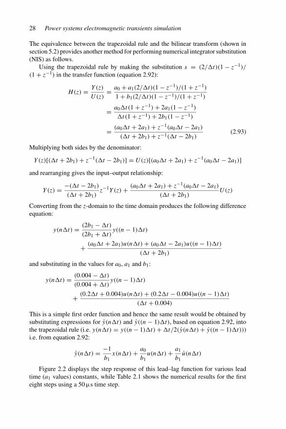
28 Power systems electromagnetic transients simulation
The equivalence between the trapezoidal rule and the bilinear transform (shown insection 5.2) provides another method for performing numerical integrator substitution(NIS) as follows.
Using the trapezoidal rule by making the substitution s = (2/�t)(1 − z−1)/
(1 + z−1) in the transfer function (equation 2.92):
H(z) = Y (z)
U(z)= a0 + a1(2/�t)(1 − z−1)/(1 + z−1)
1 + b1(2/�t)(1 − z−1)/(1 + z−1)
= a0�t(1 + z−1) + 2a1(1 − z−1)
�t(1 + z−1) + 2b1(1 − z−1)
= (a0�t + 2a1) + z−1(a0�t − 2a1)
(�t + 2b1) + z−1(�t − 2b1)(2.93)
Multiplying both sides by the denominator:
Y (z)[(�t + 2b1) + z−1(�t − 2b1)] = U(z)[(a0�t + 2a1) + z−1(a0�t − 2a1)]and rearranging gives the input–output relationship:
Y (z) = −(�t − 2b1)
(�t + 2b1)z−1Y (z) + (a0�t + 2a1) + z−1(a0�t − 2a1)
(�t + 2b1)U(z)
Converting from the z-domain to the time domain produces the following differenceequation:
y(n�t) = (2b1 − �t)
(2b1 + �t)y((n − 1)�t)
+ (a0�t + 2a1)u(n�t) + (a0�t − 2a1)u((n − 1)�t)
(�t + 2b1)
and substituting in the values for a0, a1 and b1:
y(n�t) = (0.004 − �t)
(0.004 + �t)y((n − 1)�t)
+ (0.2�t + 0.004)u(n�t) + (0.2�t − 0.004)u((n − 1)�t)
(�t + 0.004)
This is a simple first order function and hence the same result would be obtained bysubstituting expressions for y(n�t) and y((n − 1)�t), based on equation 2.92, intothe trapezoidal rule (i.e. y(n�t) = y((n − 1)�t) + �t/2(y(n�t) + y((n − 1)�t)))i.e. from equation 2.92:
y(n�t) = −1
b1x(n�t) + a0
b1u(n�t) + a1
b1u(n�t)
Figure 2.2 displays the step response of this lead–lag function for various leadtime (a1 values) constants, while Table 2.1 shows the numerical results for the firsteight steps using a 50 μs time step.
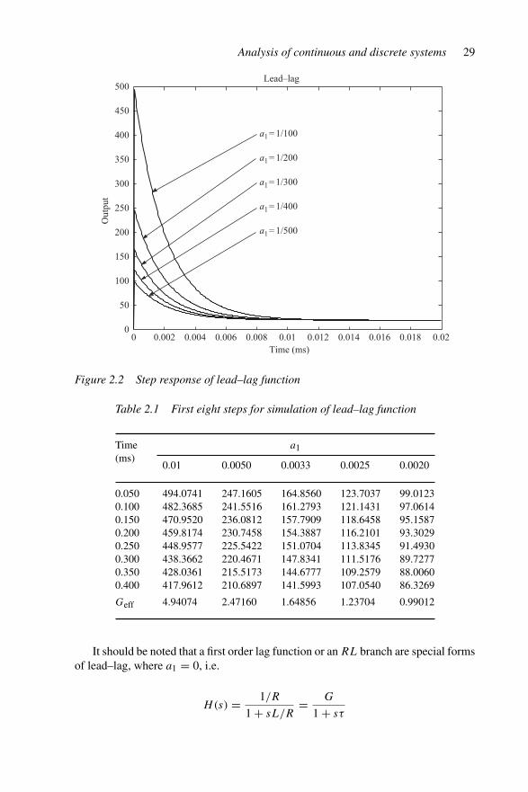
Analysis of continuous and discrete systems 29
Time (ms)
Out
put
Lead–lag
a1 = 1/100
a1 = 1/200
a1 = 1/300
a1 = 1/400
a1 = 1/500
0 0.002 0.004 0.006 0.008 0.01 0.012 0.014 0.016 0.018 0.020
50
100
150
200
250
300
350
400
450
500
Figure 2.2 Step response of lead–lag function
Table 2.1 First eight steps for simulation of lead–lag function
Time(ms)
a1
0.01 0.0050 0.0033 0.0025 0.0020
0.050 494.0741 247.1605 164.8560 123.7037 99.01230.100 482.3685 241.5516 161.2793 121.1431 97.06140.150 470.9520 236.0812 157.7909 118.6458 95.15870.200 459.8174 230.7458 154.3887 116.2101 93.30290.250 448.9577 225.5422 151.0704 113.8345 91.49300.300 438.3662 220.4671 147.8341 111.5176 89.72770.350 428.0361 215.5173 144.6777 109.2579 88.00600.400 417.9612 210.6897 141.5993 107.0540 86.3269
Geff 4.94074 2.47160 1.64856 1.23704 0.99012
It should be noted that a first order lag function or an RL branch are special formsof lead–lag, where a1 = 0, i.e.
H(s) = 1/R
1 + sL/R= G
1 + sτ
30 Power systems electromagnetic transients simulation
Thus in this case substitution of b1 = τ = L/R and a0 = 1/R produces the wellknown difference equation of an RL branch:
y(n�t) = (1 − �tR/(2L))
(1 + �tR/(2L))y((n − 1)�t)
+ �t/(2L)
(1 + �tR/(2L))(u(n�t) + u((n − 1)�t))
or in terms of G and τ
y(n�t) = (1 − �t/(2τ))
(1 + �t/(2τ))y((n − 1)�t) + (G�t/(2τ))
(1 + �t/(2τ))(u(n�t) + u((n − 1)�t))
2.3 Discrete systems
A discrete system can be represented as a z-domain function, i.e.
H(z) = Y (z)
U(z)= a0 + a1z
−1 + a2z−2 + · · · + aNz−N
1 + b1z−1 + b2z−2 + · · · + bnz−n(2.94)
When H(z) is such that ai = 0 for i = 1, 2, . . . , N but a0 �= 0 then equation 2.94represents an all-pole model (i.e. no zeros), also called an autoregressive (AR) model,as the present output depends on the output at previous time points but not on theinput at previous time points.
If bi = 0 for i = 1, 2, . . . , n except b0 �= 0, equation 2.94 represents an all-zeromodel (no poles) or moving average (MA), as the current output is an average of theprevious (and present) input but not of the previous output. In digital signal processingthis corresponds to a finite impulse response (FIR) filter.
If both poles and zeros exist then equation 2.94 represents an ARMA model,which in digital signal processing corresponds to an infinite impulse response (IIR)filter [6], i.e.
U(z)(a0 + a1z
−1 + a2z−2 + · · · + aNz−N
)
= Y (z)(
1 + b1z−1 + b2z
−2 + · · · + bnz−n
)(2.95)
Y (z) = −Y (z)(b1z
−1 + b2z−2 + · · · + bnz
−n)
+ u(z)(a0 + a1z
−1 + a2z−2 + · · · + aNz−N
)(2.96)
Transforming the last expression to the time domain, where y(k) represents the kth
time point value of y, gives:
y(k) = − (b1y(k − 1) + b2y(k − 2) + · · · + bny(k − n))
+ (a0uk + a1u(k − 1) + a2u(k − 2) + · · · + aNu(k − N)) (2.97)

Analysis of continuous and discrete systems 31
and rearranging to show the Instantaneous and History terms
y(k) =Instantaneous︷ ︸︸ ︷a0u(k) + (2.98)
History term︷ ︸︸ ︷(a1u(k − 1) + a2u(k − 2) + · · · + aNu(k − N) − b1y(k − 1) + a2y(k − 2) + · · · + any(k − n))
This equation can then be represented as a Norton equivalent as depicted in Figure 2.3.The state variable equations for a discrete system are:
x(k + 1) = [A]x(k) + [B]u(k) (2.99)
y(k + 1) = [C]x(k) + [D]u(k) (2.100)
Taking the z-transform of the state equations and combining them shows theequivalence with the continuous time counterpart. i.e.
Y (z) = H(Z)U(z) (2.101)
H(z) = [C](z[I ] − [A])−1[B] + [D] (2.102)
where [I ] is the identity matrix.The dynamic response of a discrete system is determined by the pole positions,
which for stability must be inside the unit circle in the z-plane. Figure 2.4 displaysthe impulse response for various pole positions.
IHistory
IHistory = a1u (t − Δt) + a2u (t − 2Δt) + . . . + aNu (t − NΔt)– b1 u (t − Δt) – b2u (t − Δt) – . . . + bnu (t − nΔt)
1a0
R =
Figure 2.3 Norton of a rational function in z-domain

32 Power systems electromagnetic transients simulation
1
Out
put
Out
put
Out
put
Out
put
Out
put
Out
put
Out
put
Time
Time
Time Time
Time
Time
Time
Imaginaryaxis
Unit circle
Real axis
Figure 2.4 Data sequence associated with z-plane pole locations
2.4 Relationship of continuous and discrete domains
Figure 2.5 depicts the relationships between the continuous and discrete timeprocesses as well as the s-domain and z-domain. Starting from the top left, in the timedomain a continuous function can be expressed as a high order differential equation ora group of first order (state variable) equations. The equivalent of this exists in the dis-crete time case where the output can be related to the state at only the previous step andthe input at the present and previous step. In this case the number of state variables,and hence equations, equals the order of the system. The alternative discrete timeformulation is to express the output as a function of the output and input for a numberof previous time steps (recursive formulation). In this case the number of previoustime steps required equals the order of the system. To move from continuous time todiscrete time requires a sampling process. The opposite process is a sample and hold.
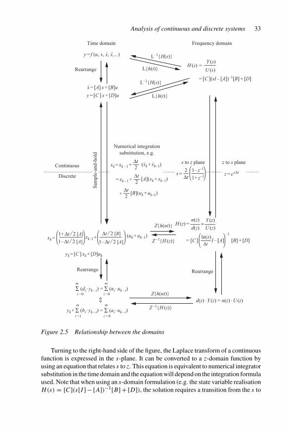
Analysis of continuous and discrete systems 33
ln(z)I – [A]) [B] + [D]
H (z)n(z)
d(z)
d(z) . Y (z) = n(z) . U (z)
Y (z)
U (z)
Δt= [C ](
==
xk = xk–1 +1+ Δt / 2 [A] Δt / 2 [B]
1– Δt / 2 [A] 1– Δt / 2 [A]
U (s)
Y (s)H (s) =
y = f (u, x, x, x,...)
z to s planes to z plane
Δt
1– z–1
1+ z–1
2s ≈ z = esΔt
.
.
..
Time domain Frequency domain
x = [A] x + [B]u
y = [C ] x + [D]u
L–1{H(s)}
L–1{H(s)}
L{h(t)}
L{h(t)}
= [C ](sI – [A])–1[B] + [D]
xk = xk – 1 +Δt2
(xk + xk–1)
Numerical integration substitution, e.g.
Rearrange
Rearrange
. .
= xk – 1 +Δt2
[A](xk + xk–1)
Δt2
[B](uk + uk–1)+
Continuous
Discrete
Sam
ple-
and-
hold
(uk + uk–1)Z –1{H (z)}
Z –1{H (z)}
Z{h(nt)}
Z{h(nt)}
yk = [C ] xk + [D]uk
Rearrange
m
i =0
m
i =0∑ (di
. yk – i) = ∑ (ni. uk – i)
m
i = 0
m
i =1yk + ∑ (bi
. yk – i) = ∑ (ai. uk – i)
–1
Figure 2.5 Relationship between the domains
Turning to the right-hand side of the figure, the Laplace transform of a continuousfunction is expressed in the s-plane. It can be converted to a z-domain function byusing an equation that relates s to z. This equation is equivalent to numerical integratorsubstitution in the time domain and the equation will depend on the integration formulaused. Note that when using an s-domain formulation (e.g. the state variable realisationH(s) = [C](s[I ]− [A])−1[B]+ [D]), the solution requires a transition from the s to
34 Power systems electromagnetic transients simulation
z-domain. Often people make this transition without realising that they have done so.The z-domain is the discrete equivalent to the s-domain. Finally the z-transform andinverse z-transform are used to go between discrete time difference equations and az-domain representation.
2.5 Summary
With the exceptions of a few auxiliary components, the electrical power systemis a continuous system, which can be represented mathematically by a system ofdifferential and algebraic equations.
A convenient form of these equations is the state variable formulation, in which asystem of n first-order linear differential equations results from an nth order system.The state variable formulation is not unique and depends on the choice of state vari-ables. The following state variable realisations have been described in this chapter:successive differentiation, controller canonical, observer canonical and diagonalcanonical.
Digital simulation is by nature a discrete time process and can only provide solu-tions for the differential and algebraic equations at discrete points in time, hence thisrequires the formulation of discrete systems. The discrete representation can alwaysbe expressed as a difference equation, where the output at a new time point is calcu-lated from the output at previous time points and the inputs at the present and previoustime points.
2.6 References
1 KAILATH, T.: ‘Linear systems’ (Prentice Hall, Englewood Cliffs, 1980)2 DeRUSSO, P. M., ROY, R. J., CLOSE, C. M. and DESROCHERS, A. A.: ‘State
variables for engineers’ (John Wiley, New York, 2nd edition, 1998)3 SMITH, J. M.: ‘Mathematical modeling and digital simulation for engineers and
scientists’ (John Wiley, New York, 2nd edition, 1987)4 OGATA, K.: ‘Modern control engineering’ (Prentice Hall International, Upper
Saddle River, N. J., 3rd edition, 1997)5 RAJAGOPALAN, V.: ‘Computer-aided analysis of power electronic system’
(Marcel Dekker, New York, 1987)6 DORF, R. C. (Ed.): ‘The electrical engineering handbook’ (CRC Press, Boca Raton,
FL, 2nd edition, 1997)
Chapter 3
State variable analysis
3.1 Introduction
State variables are the parameters of a system that completely define its energy storagestate. State variable analysis was the dominant technique in transient simulation priorto the appearance of the numerical integration substitution method.
Early state variable programs used the ‘central process’ method [1] that breaks theswitching operation down into similar consecutive topologies. This method requiresmany subroutines, each solving the set of differential equations arising from a partic-ular network topology. It has very little versatility, as only coded topologies can besimulated, thus requiring a priori knowledge of all possible circuit configurations.
The application of Kron’s tensor techniques [2] led to an elegant and efficientmethod for the solution of systems with periodically varying topology, such as ana.c.–d.c. converter. Its main advantages are more general applicability and a logicalprocedure for the automatic assembly and solution of the network equations. Thusthe programmer no longer needs to be aware of all the sets of equations describingeach particular topology.
The use of diakoptics, as proposed by Kron, considerably reduces the computa-tional burden but is subject to some restrictions on the types of circuit topology thatcan be analysed. Those restrictions, the techniques used to overcome them and thecomputer implementation of the state variable method are considered in this chapter.
3.2 Choice of state variables
State variable (or state space) analysis represents the power system by a set of firstorder differential equations, which are then solved by numerical integration. Althoughthe inductor current and capacitor voltage are the state variables normally chosen intextbooks, it is better to use the inductor’s flux linkage (φ) and capacitor’s charge (Q).Regardless of the type of numerical integration used, this variable selection reduces
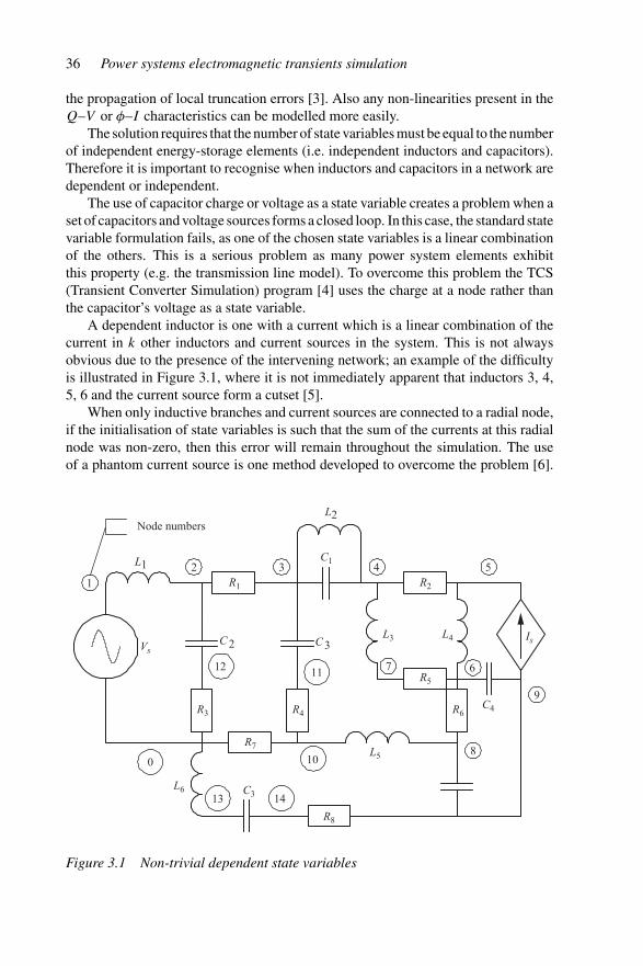
36 Power systems electromagnetic transients simulation
the propagation of local truncation errors [3]. Also any non-linearities present in theQ–V or φ–I characteristics can be modelled more easily.
The solution requires that the number of state variables must be equal to the numberof independent energy-storage elements (i.e. independent inductors and capacitors).Therefore it is important to recognise when inductors and capacitors in a network aredependent or independent.
The use of capacitor charge or voltage as a state variable creates a problem when aset of capacitors and voltage sources forms a closed loop. In this case, the standard statevariable formulation fails, as one of the chosen state variables is a linear combinationof the others. This is a serious problem as many power system elements exhibitthis property (e.g. the transmission line model). To overcome this problem the TCS(Transient Converter Simulation) program [4] uses the charge at a node rather thanthe capacitor’s voltage as a state variable.
A dependent inductor is one with a current which is a linear combination of thecurrent in k other inductors and current sources in the system. This is not alwaysobvious due to the presence of the intervening network; an example of the difficultyis illustrated in Figure 3.1, where it is not immediately apparent that inductors 3, 4,5, 6 and the current source form a cutset [5].
When only inductive branches and current sources are connected to a radial node,if the initialisation of state variables is such that the sum of the currents at this radialnode was non-zero, then this error will remain throughout the simulation. The useof a phantom current source is one method developed to overcome the problem [6].
L1
L2
L4L3
L5
L6
R1
R3 R4
R7
R6
R5
R2
R8
C1
2C 3C
C4
C3
IsVs
1
2 3 4 5
67
8
9
10
1112
0
13 14
Node numbers
Figure 3.1 Non-trivial dependent state variables
State variable analysis 37
Another approach is to choose an inductor at each node with only inductors connectedto it, and make its flux a dependent rather than a state variable.
However, each method has some disadvantage. For instance the phantom currentsource can cause large voltage spikes when trying to compensate for the inaccurateinitial condition. The partition of the inductor fluxes into state and dependent variablesis complicated and time consuming. An inductor can still be dependent even if it is notdirectly connected to a radial node of inductive branches when there is an interveningresistor/capacitor network.
The identification of state variables can be achieved by developing a node–branchincidence matrix, where the branches are ordered in a particular pattern (e.g. currentsources, inductors, voltage sources, capacitors, resistors) and Gaussian eliminationperformed. The resulting staircase columns represent state variables [3]. However,the computation required by this identification method has to be performed every timethe system topology changes. It is therefore impractical when frequently switchingpower electronic components are present. One possible way to reduce the computationburden is to separate the system into constant and frequently switching parts, usingvoltage and current sources to interface the two [7].
Two state variable programs ATOSEC [8] and TCS (Transient Converter Sim-ulator) [9], written in FORTRAN, have been used for system studies, the formerfor power electronic systems and the latter for power systems incorporating HVDCtransmission. A toolkit for MATLAB using state variable techniques has also beendeveloped.
3.3 Formation of the state equations
As already explained, the simplest method of formulating state equations is to acceptall capacitor charges and inductor fluxes as state variables. Fictitious elements, such asthe phantom current source and resistors are then added to overcome the dependencyproblem without affecting the final result significantly. However the elimination ofthe dependent variables is achieved more effectively with the transform and graphtheory methods discussed in the sections that follow.
3.3.1 The transform method
A linear transformation can be used to reduce the number of state variables. Thechange from capacitor voltage to charge at the node, mentioned in section 3.2, fallswithin this category. Consider the simple loop of three capacitors shown in Figure 3.2,where the charge at the nodes will be defined, rather than the capacitor charge.
The use of a linear transformation changes the [C] matrix from a 3 × 3 matrixwith only diagonal elements to a full 2×2 matrix. The branch–node incidence matrix,Kt
bn, is:
Ktbn =
⎡
⎣1 01 −10 1
⎤
⎦ (3.1)

38 Power systems electromagnetic transients simulation
a b
C2
C3C1
Figure 3.2 Capacitive loop
and the equation relating the three state variables to the capacitor voltages:⎛
⎝q1q2q3
⎞
⎠ =⎡
⎣C1 0 00 C2 00 0 C3
⎤
⎦
⎛
⎝v1v2v3
⎞
⎠ (3.2)
Using the connection between node and capacitor charges (i.e. equation 3.1):
(qa
qb
)=
[1 1 00 −1 1
]⎛
⎝q1q2q3
⎞
⎠ (3.3)
and ⎛
⎝v1v2v3
⎞
⎠ =⎡
⎣1 01 −10 1
⎤
⎦(
va
vb
)(3.4)
Substituting equations 3.2 and 3.4 in 3.3 yields:
(qa
qb
)=
[C1 C2 00 −C2 C3
]⎡
⎣1 01 −10 1
⎤
⎦(
va
vb
)=
[C1 + C2 −C2
−C2 C2 + C3
](va
vb
)
(3.5)Use of this transform produces a minimum set of state variables, and uses all the
capacitor values at each iteration in the integration routine. However, there is a restric-tion on the system topology that can be analysed, namely all capacitor subnetworksmust contain the reference node. For example, the circuit in Figure 3.3 (a) cannot beanalysed, as this method defines two state variables and the [C] matrix is singular andcannot be inverted. i.e.
(qa
qb
)=
[C1 −C1
−C1 C1
](va
vb
)(3.6)
This problem can be corrected by adding a small capacitor, C2, to the reference node(ground) as shown in Figure 3.3 (b). Thus the new matrix equation becomes:
(qa
qb
)=
[C1 + C2 −C1
−C1 C1
](va
vb
)(3.7)
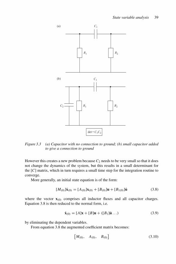
State variable analysis 39
C1
R1 R2
C1
R1C2 R2
det = C1C2
(a)
(b)
Figure 3.3 (a) Capacitor with no connection to ground; (b) small capacitor addedto give a connection to ground
However this creates a new problem because C2 needs to be very small so that it doesnot change the dynamics of the system, but this results in a small determinant forthe [C] matrix, which in turn requires a small time step for the integration routine toconverge.
More generally, an initial state equation is of the form:
[M(0)]x(0) = [A(0)]x(0) + [B(0)]u + [B1(0)]u (3.8)
where the vector x(0) comprises all inductor fluxes and all capacitor charges.Equation 3.8 is then reduced to the normal form, i.e.
x(0) = [A]x + [B]u + ([B1]u . . .) (3.9)
by eliminating the dependent variables.From equation 3.8 the augmented coefficient matrix becomes:
[M(0), A(0), B(0)
](3.10)

40 Power systems electromagnetic transients simulation
Elementary row operations are performed on the augmented coefficient matrix toreduce it to echelon form [3]. If M(0) is non-singular the result will be an upper trian-gular matrix with non-zero diagonal elements. Further elementary row operations willreduce M(0) to the identity matrix. This is equivalent to pre-multiplying equation 3.10by M−1
(0) , i.e. reducing it to the form
[I, A, B
](3.11)
If in the process of reducing to row echelon form the j th row in the first block becomesa row of all zeros then M(0) was singular. In this case three conditions can occur.
• The j th row in the other two submatrices are also zero, in which case the networkhas no unique solution as there are fewer constraint equations than unknowns.
• The j th row elements in the second submatrix (A) are zero, which gives an incon-sistent network, as the derivatives of state variables relate only to input sources,which are supposed to be independent.
• The j th row elements in the second submatrix (originally [A(0)]) are not zero(regardless of the third submatrix). Hence the condition is [0, 0, . . . , 0]x =[aj1, aj2, . . . , ajn]x + [bj1, bj2, . . . , bjm]u. In this case there is at least one non-zero value ajk , which allows state variable xk to be eliminated. Rearranging theequation associated with the kth row of the augmented matrix 3.10 gives:
xk = −1
ajk
(aj1x1 + aj2x2 + · · · + ajk−1xk−1 + ajk+1xk+1 + · · · + ajnxn
+ bj1u1 + bj2u2 + · · · + bjmum) (3.12)
Substituting this for xk in equation 3.8 and eliminating the equation associated withxk yields:
[M(1)]x(1) = [A(1)]x(1) + [B(1)]u + [B(1)]u (3.13)
This process is repeatedly applied until all variables are linearly independent andhence the normal form of state equation is achieved.
3.3.2 The graph method
This method solves the problem in two stages. In the first stage a tree, T, is foundwith a given preference to branch type and value for inclusion in the tree. The secondstage forms the loop matrix associated with the chosen tree T.
The graph method determines the minimal and optimal state variables. This canbe achieved either by:
(i) elementary row operations on the connection matrix, or(ii) path search through a connection table.
The first approach consists of rearranging the rows of the incidence (or connection)matrix to correspond to the preference required, as shown in Figure 3.4. The dimensionof the incidence matrix is n × b, where n is the number of nodes (excluding the
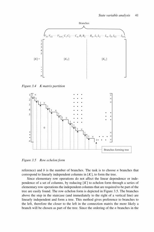
State variable analysis 41
12345
n
VS1 VS2. . . VS nVs
C1 C2. . . Cnc R1 R2
. . . Rnr L1 L2. . . Lnr IS1 IS2
. . . IS nIs
[K] = [KT ] [KL ]
Branches
Figure 3.4 K matrix partition
Branches forming tree
1 11
11
11
1
11
1
11
1
2
3
4
5
n•••
0
• • •
• • •
• • •
• • •
• • •
• • •
• • •
• • •
• • •• • •
×
×
×
×
×
××××
×××
•
•
•
•
•
•
Figure 3.5 Row echelon form
reference) and b is the number of branches. The task is to choose n branches thatcorrespond to linearly independent columns in [K], to form the tree.
Since elementary row operations do not affect the linear dependence or inde-pendence of a set of columns, by reducing [K] to echelon form through a series ofelementary row operations the independent columns that are required to be part of thetree are easily found. The row echelon form is depicted in Figure 3.5. The branchesabove the step in the staircase (and immediately to the right of a vertical line) arelinearly independent and form a tree. This method gives preference to branches tothe left, therefore the closer to the left in the connection matrix the more likely abranch will be chosen as part of the tree. Since the ordering of the n branches in the
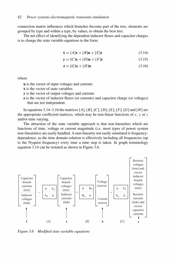
42 Power systems electromagnetic transients simulation
connection matrix influences which branches become part of the tree, elements aregrouped by type and within a type, by values, to obtain the best tree.
The net effect of identifying the dependent inductor fluxes and capacitor chargesis to change the state variable equations to the form:
x = [A]x + [B]u + [E]z (3.14)
y = [C]x + [D]u + [F ]z (3.15)
z = [G]x + [H ]u (3.16)
where
u is the vector of input voltages and currentsx is the vector of state variablesy is the vector of output voltages and currentsz is the vector of inductor fluxes (or currents) and capacitor charge (or voltages)
that are not independent.
In equations 3.14–3.16 the matrices [A], [B], [C], [D], [E], [F ], [G] and [H ] arethe appropriate coefficient matrices, which may be non-linear functions of x, y or z
and/or time varying.The attraction of the state variable approach is that non-linearities which are
functions of time, voltage or current magnitude (i.e. most types of power systemnon-linearities) are easily handled. A non-linearity not easily simulated is frequency-dependence, as the time domain solution is effectively including all frequencies (upto the Nyquist frequency) every time a time step is taken. In graph terminologyequation 3.14 can be restated as shown in Figure 3.6.
Capacitorbranchcurrents
(tree)
Inductorvoltages
(link)
=0
0
AL
AT+
Capacitorbranch
voltages(tree)
Inductorcurrents(link)
0
0
BL
BT
+0
0
EL
ET
Voltagesources
Currentsources
Resistorvoltages
(tree) and excess
inductorbranch
voltages(tree)
Resistorcurrents
(link) and excess
capacitorcurrents
x [A] [B] [E ].
x u z
Figure 3.6 Modified state variable equations

State variable analysis 43
3.4 Solution procedure
Figure 3.7 shows the structure of the state variable solution. Central to the solutionprocedure is the numerical integration technique. Among the possible alternatives,
Integrate
Initial estimate of state variable derivatives
Δt2
Has convergence been obtained?
Has maximum number of iterations
been reached?
Halve step size
Use state equation to obtain state variable derivatives
Yes
No
Yes
No
Too many step- halvings?
No
STOP
Yes
Small number of iterations required?
Large number of iterations required?
Increase time step by 10%
Decrease time step by 10%
No
No
Calculate dependent variables
Advance time
(xt − Δt + xt)
xt= xt−Δt
xt= xt−Δt +
xt = [A]xt + [B]ut
yt = [C ]xt + [D]ut
Yes
Yes
.
. .
.
.
Figure 3.7 Flow chart for state variable analysis
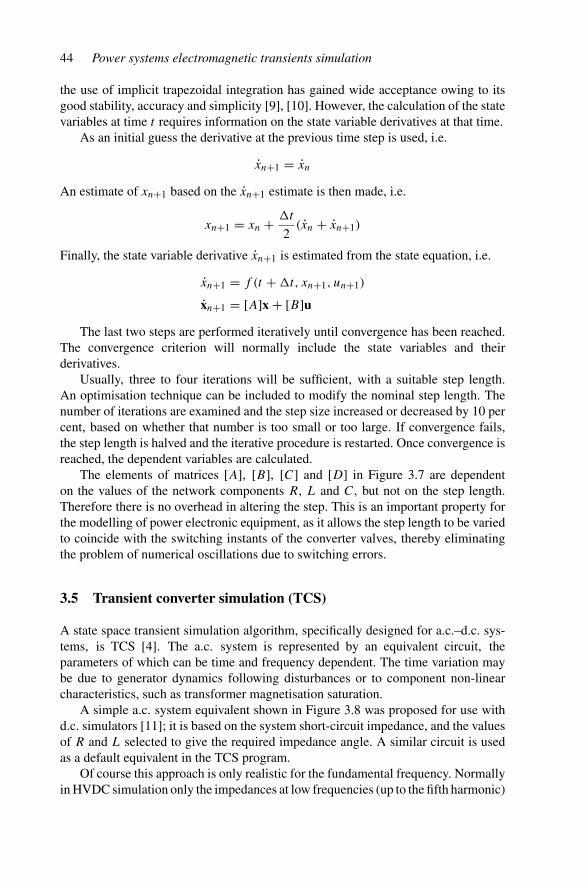
44 Power systems electromagnetic transients simulation
the use of implicit trapezoidal integration has gained wide acceptance owing to itsgood stability, accuracy and simplicity [9], [10]. However, the calculation of the statevariables at time t requires information on the state variable derivatives at that time.
As an initial guess the derivative at the previous time step is used, i.e.
xn+1 = xn
An estimate of xn+1 based on the xn+1 estimate is then made, i.e.
xn+1 = xn + �t
2(xn + xn+1)
Finally, the state variable derivative xn+1 is estimated from the state equation, i.e.
xn+1 = f (t + �t, xn+1, un+1)
xn+1 = [A]x + [B]uThe last two steps are performed iteratively until convergence has been reached.
The convergence criterion will normally include the state variables and theirderivatives.
Usually, three to four iterations will be sufficient, with a suitable step length.An optimisation technique can be included to modify the nominal step length. Thenumber of iterations are examined and the step size increased or decreased by 10 percent, based on whether that number is too small or too large. If convergence fails,the step length is halved and the iterative procedure is restarted. Once convergence isreached, the dependent variables are calculated.
The elements of matrices [A], [B], [C] and [D] in Figure 3.7 are dependenton the values of the network components R, L and C, but not on the step length.Therefore there is no overhead in altering the step. This is an important property forthe modelling of power electronic equipment, as it allows the step length to be variedto coincide with the switching instants of the converter valves, thereby eliminatingthe problem of numerical oscillations due to switching errors.
3.5 Transient converter simulation (TCS)
A state space transient simulation algorithm, specifically designed for a.c.–d.c. sys-tems, is TCS [4]. The a.c. system is represented by an equivalent circuit, theparameters of which can be time and frequency dependent. The time variation maybe due to generator dynamics following disturbances or to component non-linearcharacteristics, such as transformer magnetisation saturation.
A simple a.c. system equivalent shown in Figure 3.8 was proposed for use withd.c. simulators [11]; it is based on the system short-circuit impedance, and the valuesof R and L selected to give the required impedance angle. A similar circuit is usedas a default equivalent in the TCS program.
Of course this approach is only realistic for the fundamental frequency. Normallyin HVDC simulation only the impedances at low frequencies (up to the fifth harmonic)
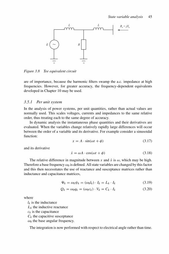
State variable analysis 45
~E R
L L Rs + jXs
Figure 3.8 Tee equivalent circuit
are of importance, because the harmonic filters swamp the a.c. impedance at highfrequencies. However, for greater accuracy, the frequency-dependent equivalentsdeveloped in Chapter 10 may be used.
3.5.1 Per unit system
In the analysis of power systems, per unit quantities, rather than actual values arenormally used. This scales voltages, currents and impedances to the same relativeorder, thus treating each to the same degree of accuracy.
In dynamic analysis the instantaneous phase quantities and their derivatives areevaluated. When the variables change relatively rapidly large differences will occurbetween the order of a variable and its derivative. For example consider a sinusoidalfunction:
x = A · sin(ωt + φ) (3.17)
and its derivativex = ωA · cos(ωt + φ) (3.18)
The relative difference in magnitude between x and x is ω, which may be high.Therefore a base frequency ω0 is defined. All state variables are changed by this factorand this then necessitates the use of reactance and susceptance matrices rather thaninductance and capacitance matrices,
�k = ω0ψk = (ω0lk) · Ik = Lk · Ik (3.19)
Qk = ω0qk = (ω0ck) · Vk = Ck · Ik (3.20)
wherelk is the inductanceLk the inductive reactanceck is the capacitanceCk the capacitive susceptanceω0 the base angular frequency.
The integration is now performed with respect to electrical angle rather than time.
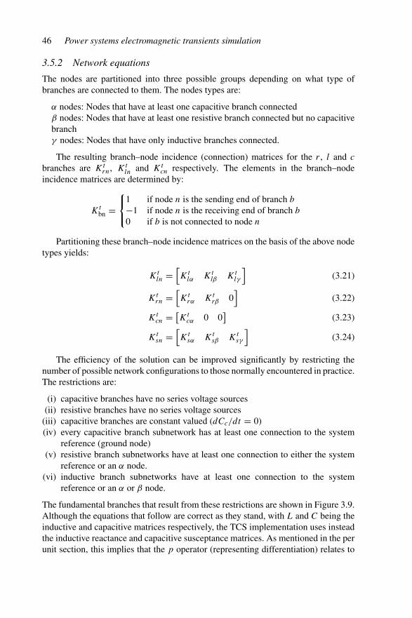
46 Power systems electromagnetic transients simulation
3.5.2 Network equations
The nodes are partitioned into three possible groups depending on what type ofbranches are connected to them. The nodes types are:
α nodes: Nodes that have at least one capacitive branch connectedβ nodes: Nodes that have at least one resistive branch connected but no capacitivebranchγ nodes: Nodes that have only inductive branches connected.
The resulting branch–node incidence (connection) matrices for the r , l and c
branches are Ktrn, Kt
ln and Ktcn respectively. The elements in the branch–node
incidence matrices are determined by:
Ktbn =
⎧⎨
⎩
1 if node n is the sending end of branch b
−1 if node n is the receiving end of branch b
0 if b is not connected to node n
Partitioning these branch–node incidence matrices on the basis of the above nodetypes yields:
Ktln =
[Kt
lα Ktlβ Kt
lγ
](3.21)
Ktrn =
[Kt
rα Ktrβ 0
](3.22)
Ktcn = [
Ktcα 0 0
](3.23)
Ktsn =
[Kt
sα Ktsβ Kt
sγ
](3.24)
The efficiency of the solution can be improved significantly by restricting thenumber of possible network configurations to those normally encountered in practice.The restrictions are:
(i) capacitive branches have no series voltage sources(ii) resistive branches have no series voltage sources
(iii) capacitive branches are constant valued (dCc/dt = 0)(iv) every capacitive branch subnetwork has at least one connection to the system
reference (ground node)(v) resistive branch subnetworks have at least one connection to either the system
reference or an α node.(vi) inductive branch subnetworks have at least one connection to the system
reference or an α or β node.
The fundamental branches that result from these restrictions are shown in Figure 3.9.Although the equations that follow are correct as they stand, with L and C being theinductive and capacitive matrices respectively, the TCS implementation uses insteadthe inductive reactance and capacitive susceptance matrices. As mentioned in the perunit section, this implies that the p operator (representing differentiation) relates to
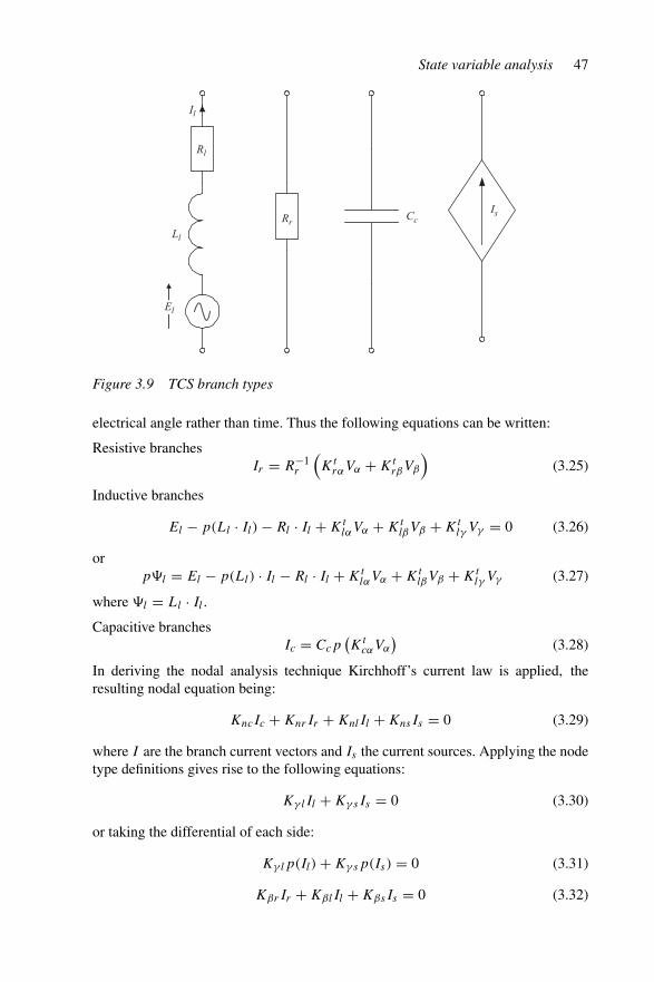
State variable analysis 47
Rl
Ll
El
Il
RrCc
Is
Figure 3.9 TCS branch types
electrical angle rather than time. Thus the following equations can be written:
Resistive branchesIr = R−1
r
(Kt
rαVα + KtrβVβ
)(3.25)
Inductive branches
El − p(Ll · Il) − Rl · Il + KtlαVα + Kt
lβVβ + Ktlγ Vγ = 0 (3.26)
orp�l = El − p(Ll) · Il − Rl · Il + Kt
lαVα + KtlβVβ + Kt
lγ Vγ (3.27)
where �l = Ll · Il .
Capacitive branchesIc = Ccp
(Kt
cαVα
)(3.28)
In deriving the nodal analysis technique Kirchhoff’s current law is applied, theresulting nodal equation being:
KncIc + KnrIr + KnlIl + KnsIs = 0 (3.29)
where I are the branch current vectors and Is the current sources. Applying the nodetype definitions gives rise to the following equations:
Kγ lIl + KγsIs = 0 (3.30)
or taking the differential of each side:
Kγ lp(Il) + Kγsp(Is) = 0 (3.31)
KβrIr + KβlIl + KβsIs = 0 (3.32)

48 Power systems electromagnetic transients simulation
KαcIc + KαrIr + KαlIl + KαsIs = 0 (3.33)
Pre-multiplying equation 3.28 by Ktαc and substituting into equation 3.33 yields:
p(Qα) = −KαlIl + KαrIr − KαrIr − KαsIs (3.34)
whereQα = CαVα
C−1α =
(KαcCcK
tcα
)−1.
The dependent variables Vβ , Vγ and Ir can be entirely eliminated from the solutionso only Il , Vα and the input variables are explicit in the equations to be integrated.This however is undesirable due to the resulting loss in computational efficiency eventhough it reduces the overall number of equations. The reasons for the increasedcomputational burden are:
• loss of matrix sparsity• incidence matrices no longer have values of −1, 0 or 1. This therefore requires
actual multiplications rather than simple additions or subtractions when calculatinga matrix product.
• Some quantities are not directly available, making it time-consuming to recalculateif it is needed at each time step.
Therefore Vβ , Vγ and Ir are retained and extra equations derived to evaluate thesedependent variables. To evaluate Vβ equation 3.25 is pre-multiplied by Kβr and thencombined with equation 3.32 to give:
Vβ = −Rβ
(KβsIs + KβlIl + KβrR
−1r Kt
rαVα
)(3.35)
where Rβ = (KβrR−1r Kt
rβ)−1.Pre-multiplying equation 3.26 by Kγ l and applying to equation 3.31 gives the
following expression for Vγ :
Vγ = −Lγ Kγsp(Is) − Lγ Kγ lL−1γ
(El − p(Ll) · Il − RlIl + Kt
lαVα + KtlβVβ
)
(3.36)where Lγ = (Kγ lL
−1l Kt
lγ )−1 and Ir is evaluated by using equation 3.25.Once the trapezoidal integration has converged the sequence of solutions for a time
step is as follows: the state related variables are calculated followed by the dependentvariables and lastly the state variable derivatives are obtained from the state equation.State related variables:
Il = L−1l �l (3.37)
Vα = C−1α Qα (3.38)
State variable analysis 49
Dependent variables:
Vβ = −Rβ
(KβsIs + KβlIl + KβrR
−1r Kt
rαVα
)(3.39)
Ir = R−1r
(Kt
rαVα + KtrβVβ
)(3.40)
Vγ = −Lγ Kγsp(Is) − Lγ Kγ lL−1l
(El − p(Ll) · Il − RlIl + Kt
lαVα + KtlβVβ
)
(3.41)
State equations:
p�l = El − p(Ll) · Il − Rl · Il + KtlαVα + Kt
lβVβ + Ktlγ Vγ (3.42)
p(Qα) = −KαlIl + KαrIr − KαrIr − KαsIs (3.43)
whereC−1
α = (KαcCcKtcα)−1
Lγ = (Kγ lL−1l Kt
lγ )−1
Rβ = (KβrR−1r Kt
rβ)−1.
3.5.3 Structure of TCS
To reduce the data input burden TCS suggests an automatic procedure, whereby thecollation of the data into the full network is left to the computer. A set of controlparameters provides all the information needed by the program to expand a givencomponent data and to convert it to the required form. The component data set con-tains the initial current information and other parameters relevant to the particularcomponent.
For example, for the converter bridges this includes the initial d.c. current, thedelay and extinction angles, time constants for the firing control system, the smooth-ing reactor, converter transformer data, etc. Each component is then systematicallyexpanded into its elementary RLC branches and assigned appropriate node num-bers. Cross-referencing information is created relating the system busbars to thosenode numbers. The node voltages and branch currents are initialised to their specificinstantaneous phase quantities of busbar voltages and line currents respectively. Ifthe component is a converter, the bridge valves are set to their conducting states fromknowledge of the a.c. busbar voltages, the type of converter transformer connectionand the set initial delay angle.
The procedure described above, when repeated for all components, generatesthe system matrices in compact form with their indexing information, assigns nodenumbers for branch lists and initialises relevant variables in the system.
Once the system and controller data are assembled, the system is ready to beginexecution. In the data file, the excitation sources and control constraints are enteredfollowed by the fault specifications. The basic program flow chart is shown inFigure 3.10. For a simulation run, the input could be either from the data file orfrom a previous snapshot (stored at the end of a run).

50 Power systems electromagnetic transients simulation
Start
Input data and establish network equations
Input fault description
Initialise the network and controls
Monitor and control converter operation
Any switching?Modify equations and
produce output
Time variant inductance?
Update nodal inductance matrix
Solve iteratively network equations and control system for one time
step. Optimise Δt.
Advance time step by Δt (if requiredlimit to fall on next discontinuity)
Time for output?
Time for fault?
End of study?
Store all variables and state information
Stop
Produce output
Modify equations
Yes
Yes
Yes
No
No
No
No
No
Yes
Yes
Figure 3.10 TCS flow chart

State variable analysis 51
Simple control systems can be modelled by sequentially assembling the modularbuilding blocks available. Control block primitives are provided for basic arithmeticsuch as addition, multiplication and division, an integrator, a differentiator, pole–zeroblocks, limiters, etc. The responsibility to build a useful continuous control system isobviously left to the user.
At each stage of the integration process, the converter bridge valves are tested forextinction, voltage crossover and conditions for firing. If indicated, changes in thevalve states are made and the control system is activated to adjust the phase of firing.Moreover, when a valve switching occurs, the network equations and the connectionmatrix are modified to represent the new conditions.
During each conduction interval the circuit is solved by numerical integration ofthe state space model for the appropriate topology, as described in section 3.4.
3.5.4 Valve switchings
The step length is modified to fall exactly on the time required for turning ON switches.As some events, such as switching of diodes and thyristors, cannot be predicted thesolution is interpolated back to the zero crossing. At each switching instance twosolutions are obtained one immediately before and the other immediately after theswitch changes state.
Hence, the procedure is to evaluate the system immediately prior to switching byrestricting the time step or interpolating back. The connection matrices are modifiedto reflect the switch changing state, and the system resolved for the same time pointusing the output equation. The state variables are unchanged, as inductor flux (orcurrent) and capacitor charge (or voltage) cannot change instantaneously. Inductorvoltage and capacitor current can exhibit abrupt changes due to switching.
Connection matrices updated and dependent variables re-evaluated
Step length adjusted to fall
on firing instant
Step lengthadjusted to turn-off instant
Connection matrices updated and dependentvariables re-evaluated
Figure 3.11 Switching in state variable program
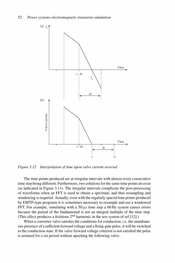
52 Power systems electromagnetic transients simulation
tx
tx t2
Δt
Δt
Il
t – Δt
t – Δt
t
Time
Time
Val
ve c
urre
nt
(a)
(b)
Figure 3.12 Interpolation of time upon valve current reversal
The time points produced are at irregular intervals with almost every consecutivetime step being different. Furthermore, two solutions for the same time points do exist(as indicated in Figure 3.11). The irregular intervals complicate the post-processingof waveforms when an FFT is used to obtain a spectrum, and thus resampling andwindowing is required. Actually, even with the regularly spaced time points producedby EMTP-type programs it is sometimes necessary to resample and use a windowedFFT. For example, simulating with a 50 μs time step a 60 Hz system causes errorsbecause the period of the fundamental is not an integral multiple of the time step.(This effect produces a fictitious 2nd harmonic in the test system of ref [12].)
When a converter valve satisfies the conditions for conduction, i.e. the simultane-ous presence of a sufficient forward voltage and a firing-gate pulse, it will be switchedto the conduction state. If the valve forward voltage criterion is not satisfied the pulseis retained for a set period without upsetting the following valve.
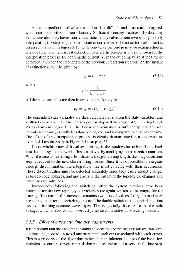
State variable analysis 53
Accurate prediction of valve extinctions is a difficult and time-consuming taskwhich can degrade the solution efficiency. Sufficient accuracy is achieved by detectingextinctions after they have occurred, as indicated by valve current reversal; by linearlyinterpolating the step length to the instant of current zero, the actual turn-off instant isassessed as shown in Figure 3.12. Only one valve per bridge may be extinguished atany one time, and the earliest extinction over all the bridges is always chosen for theinterpolation process. By defining the current (I ) in the outgoing valve at the time ofdetection (t), when the step length of the previous integration step was �t , the instantof extinction tx will be given by:
tx = t − �tz (3.44)
where
z = it
it − it−�t
All the state variables are then interpolated back to tx by
vx = vt = z(vt − vt−�t ) (3.45)
The dependent state variables are then calculated at tx from the state variables, andwritten to the output file. The next integration step will then begin at tx with step length�t as shown in Figure 3.12. This linear approximation is sufficiently accurate overperiods which are generally less than one degree, and is computationally inexpensive.The effect of this interpolation process is clearly demonstrated in a case with anextended 1 ms time step in Figure 3.14 on page 55.
Upon switching any of the valves, a change in the topology has to be reflected backinto the main system network. This is achieved by modifying the connection matrices.When the time to next firing is less than the integration step length, the integration timestep is reduced to the next closest firing instant. Since it is not possible to integratethrough discontinuities, the integration time must coincide with their occurrence.These discontinuities must be detected accurately since they cause abrupt changesin bridge-node voltages, and any errors in the instant of the topological changes willcause inexact solutions.
Immediately following the switching, after the system matrices have beenreformed for the new topology, all variables are again written to the output file fortime tx . The output file therefore contains two sets of values for tx , immediatelypreceding and after the switching instant. The double solution at the switching timeassists in forming accurate waveshapes. This is specially the case for the d.c. sidevoltage, which almost contains vertical jump discontinuities at switching instants.
3.5.5 Effect of automatic time step adjustments
It is important that the switching instants be identified correctly, first for accurate sim-ulations and, second, to avoid any numerical problems associated with such errors.This is a property of the algorithm rather than an inherent feature of the basic for-mulation. Accurate converter simulation requires the use of a very small time step,

54 Power systems electromagnetic transients simulation
where the accuracy is only achieved by correctly reproducing the appropriate discon-tinuities. A smaller step length is not only needed for accurate switching but also forthe simulation of other non-linearities, such as in the case of transformer saturation,around the knee point, to avoid introducing hysteresis due to overstepping. In thesaturated region and the linear regions, a larger step is acceptable.
On the other hand, state variable programs, and TCS in particular, have the facilityto adapt to a variable step length operation. The dynamic location of a discontinuitywill force the step length to change between the maximum and minimum step sizes.The automatic step length adjustment built into the TCS program takes into accountmost of the influencing factors for correct performance. As well as reducing the steplength upon the detection of a discontinuity, TCS also reduces the forthcoming step inanticipation of events such as an incoming switch as decided by the firing controller,the time for fault application, closing of a circuit breaker, etc.
To highlight the performance of the TCS program in this respect, a comparison ismade with an example quoted as a feature of the NETOMAC program [13]. The exam-ple refers to a test system consisting of an ideal 60 Hz a.c. system (EMF sources) feed-ing a six-pulse bridge converter (including the converter transformer and smoothingreactor) terminated by a d.c. source; the firing angle is 25 degrees. Figure 3.13 showsthe valve voltages and currents for 50 μs and 1 ms (i.e. 1 and 21 degrees) time stepsrespectively. The system has achieved steady state even with steps 20 times larger.
The progressive time steps are illustrated by the dots on the curves inFigure 3.13(b), where interpolation to the instant of a valve current reversal is madeand from which a half time step integration is carried out. The next step reverts backto the standard trapezoidal integration until another discontinuity is encountered.
A similar case with an ideal a.c. system terminated with a d.c. source was simulatedusing TCS. A maximum time step of 1 ms was used also in this case. Steady statewaveforms of valve voltage and current derived with a 1 ms time step, shown inFigure 3.14, illustrate the high accuracy of TCS, both in detection of the switching
1
1
1
Val
ve v
olta
geV
alve
cur
rent
(a) (b)
Figure 3.13 NETOMAC simulation responses: (a) 50 μs time step; (b) 1 μs timestep
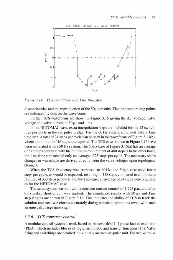
State variable analysis 55
Time
per
unit
valve 1 voltage; valve 1 current
–1.5
–1
–0.5
0
0.5
1
1.5
Figure 3.14 TCS simulation with 1 ms time step
discontinuities and the reproduction of the 50 μs results. The time step tracing pointsare indicated by dots on the waveforms.
Further TCS waveforms are shown in Figure 3.15 giving the d.c. voltage, valvevoltage and valve current at 50 μs and 1 ms.
In the NETOMAC case, extra interpolation steps are included for the 12 switch-ings per cycle in the six pulse bridge. For the 60 Hz system simulated with a 1 mstime step, a total of 24 steps per cycle can be seen in the waveforms of Figure 3.13(b),where a minimum of 16 steps are required. The TCS cases shown in Figure 3.15 havebeen simulated with a 50 Hz system. The 50 μs case of Figure 3.15(a) has an averageof 573 steps per cycle with the minimum requirement of 400 steps. On the other hand,the 1 ms time step needed only an average of 25 steps per cycle. The necessary sharpchanges in waveshape are derived directly from the valve voltages upon topologicalchanges.
When the TCS frequency was increased to 60 Hz, the 50 μs case used fewersteps per cycle, as would be expected, resulting in 418 steps compared to a minimumrequired of 333 steps per cycle. For the 1 ms case, an average of 24 steps were required,as for the NETOMAC case.
The same system was run with a constant current control of 1.225 p.u., and after0.5 s a d.c. short-circuit was applied. The simulation results with 50 μs and 1 msstep lengths are shown in Figure 3.16. This indicates the ability of TCS to track thesolution and treat waveforms accurately during transient operations (even with suchan unusually large time step).
3.5.6 TCS converter control
A modular control system is used, based on Ainsworth’s [14] phase-locked oscillator(PLO), which includes blocks of logic, arithmetic and transfer functions [15]. Valvefiring and switchings are handled individually on each six-pulse unit. For twelve-pulse
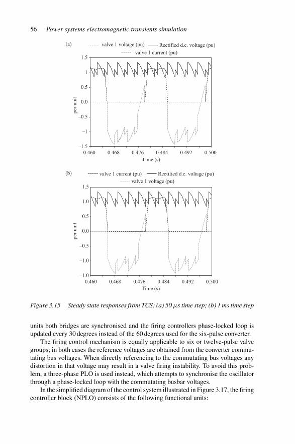
56 Power systems electromagnetic transients simulation
per
unit
per
unit
0.460 0.468 0.476 0.484 0.492 0.500Time (s)
valve 1 voltage (pu) Rectified d.c. voltage (pu)
valve 1 current (pu)
0.460 0.468 0.476 0.484 0.492 0.500Time (s)
valve 1 current (pu) Rectified d.c. voltage (pu)
valve 1 voltage (pu)
1.5
1
0.5
0.0
–0.5
–1
–1.5
–1.0
–1.0
–0.5
0.0
0.5
1.0
1.5
(a)
(b)
Figure 3.15 Steady state responses from TCS: (a) 50 μs time step; (b) 1 ms time step
units both bridges are synchronised and the firing controllers phase-locked loop isupdated every 30 degrees instead of the 60 degrees used for the six-pulse converter.
The firing control mechanism is equally applicable to six or twelve-pulse valvegroups; in both cases the reference voltages are obtained from the converter commu-tating bus voltages. When directly referencing to the commutating bus voltages anydistortion in that voltage may result in a valve firing instability. To avoid this prob-lem, a three-phase PLO is used instead, which attempts to synchronise the oscillatorthrough a phase-locked loop with the commutating busbar voltages.
In the simplified diagram of the control system illustrated in Figure 3.17, the firingcontroller block (NPLO) consists of the following functional units:

State variable analysis 57
Time(s)
d.c. fault application Rectified d.c. voltage (pu)
d.c. current (pu)
0.48 0.50 0.52 0.54 0.56 0.58 0.60
Time(s)
d.c. fault application Rectified d.c. voltage (pu)
d.c. current (pu)
–2.50
–1.25
0.00
1.25
2.50
–2.50
–1.25
0.00
1.25
2.50
0.48 0.50 0.52 0.54 0.56 0.58 0.60
(a)
(b)
Figure 3.16 Transient simulation with TCS for a d.c. short-circuit at 0.5 s: (a) 1 mstime step; (b) 50 μs time step
(i) a zero-crossing detector(ii) a.c. system frequency measurement
(iii) a phase-locked oscillator(iv) firing pulse generator and synchronising mechanism(v) firing angle (α) and extinction angle (γ ) measurement unit.
Zero-crossover points are detected by the change of sign of the reference volt-ages and multiple crossings are avoided by allowing a space between the crossings.Distortion in the line voltage can create difficulties in zero-crossing detection, andtherefore the voltages are smoothed before being passed to the zero-crossing detector.
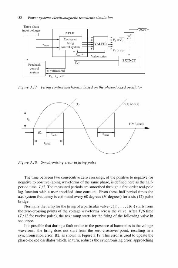
58 Power systems electromagnetic transients simulation
NPLO
VALFIR
EXTNCT
Three phase input voltages
Feedbackcontrolsystem
�order
�, � measured
Vdc , Idc , etc.
Ton, �
Toff
P6 or P12
P1 or P7Converterfiring
control system
Valve states
Figure 3.17 Firing control mechanism based on the phase-locked oscillator
�order �order
�actual
T0
B2
c (1) c (1) or c (7)
TIME (rad)
Figure 3.18 Synchronising error in firing pulse
The time between two consecutive zero crossings, of the positive to negative (ornegative to positive) going waveforms of the same phase, is defined here as the half-period time, T/2. The measured periods are smoothed through a first order real-polelag function with a user-specified time constant. From these half-period times thea.c. system frequency is estimated every 60 degrees (30 degrees) for a six (12) pulsebridge.
Normally the ramp for the firing of a particular valve (c(1), . . . , c(6)) starts fromthe zero-crossing points of the voltage waveforms across the valve. After T/6 time(T/12 for twelve pulse), the next ramp starts for the firing of the following valve insequence.
It is possible that during a fault or due to the presence of harmonics in the voltagewaveform, the firing does not start from the zero-crossover point, resulting in asynchronisation error, B2, as shown in Figure 3.18. This error is used to update thephase-locked oscillator which, in turn, reduces the synchronising error, approaching

State variable analysis 59
zero at the steady state condition. The synchronisation error is recalculated every60 deg for the six-pulse bridge.
The firing angle order (αorder) is converted to a level to detect the firing instant asa function of the measured a.c. frequency by
T0 = αorder(rad.)
fac(p.u.)(3.46)
As soon as the ramp c(n) reaches the set level specified by T0, as shown inFigure 3.18, valve n is fired and the firing pulse is maintained for 120 degrees. Uponhaving sufficient forward voltage with the firing-pulse enabled, the valve is switchedon and the firing angle recorded as the time interval from the last voltage zero crossingdetected for this valve.
At the beginning of each time-step, the valves are checked for possible extinc-tions. Upon detecting a current reversal, a valve is extinguished and its extinctionangle counter is reset. Subsequently, from the corresponding zero-crossing instant,its extinction angle is measured, e.g. at valve 1 zero crossing, γ2 is measured, andso on. (Usually, the lowest gamma angle measured for the converter is fed back tothe extinction angle controller.) If the voltage zero-crossover points do not fall on thetime step boundaries, a linear interpolation is used to derive them. As illustrated inFigure 3.17, the NPLO block coordinates the valve-firing mechanism, and VALFIRreceives the firing pulses from NPLO and checks the conditions for firing the valves.If the conditions are met, VALFIR switches on the next incoming valve and measuresthe firing angle, otherwise it calculates the earliest time for next firing to adjust thestep length. Valve currents are checked for extinction in EXTNCT and interpolationof all state variables is carried out. The valve’s turn-on time is used to calculate thefiring angle and the off time is used for the extinction angle.
By way of example, Figure 3.19 shows the response to a step change of d.c.current in the test system used earlier in this section.
3.6 Example
To illustrate the use of state variable analysis the simple RLC circuit of Figure 3.20is used (R = 20.0 �, L = 6.95 mH and C = 1.0 μF), where the switch is closed at0.1 ms. Choosing x1 = vC and x2 = iL then the state variable equation is:
(x1x2
)=
⎡
⎢⎣
01
C−1
L
−R
L
⎤
⎥⎦(
x1x2
)+
⎛
⎝01
L
⎞
⎠ES (3.47)
The FORTRAN code for this example is given in Appendix G.1. Figure 3.21 displaysthe response from straight application of the state variable analysis using a 0.05 mstime step. The first plot compares the response with the analytic answer. The resonantfrequency for this circuit is 1909.1 Hz (or a period of 0.5238 ms), hence having approx-imately 10 points per cycle. The second plot shows that the step length remained at
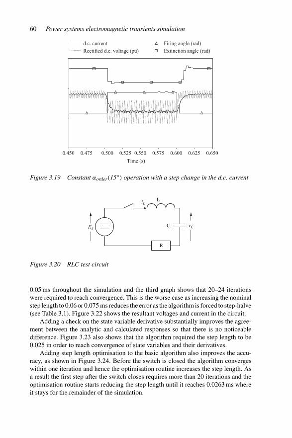
60 Power systems electromagnetic transients simulation
Time (s)
d.c. current
Rectified d.c. voltage (pu)
Firing angle (rad)
Extinction angle (rad)
0.450 0.475 0.500 0.525 0.550 0.575 0.600 0.625 0.650
Figure 3.19 Constant αorder(15◦) operation with a step change in the d.c. current
iL
ESvC
L
R
C
Figure 3.20 RLC test circuit
0.05 ms throughout the simulation and the third graph shows that 20–24 iterationswere required to reach convergence. This is the worse case as increasing the nominalstep length to 0.06 or 0.075 ms reduces the error as the algorithm is forced to step-halve(see Table 3.1). Figure 3.22 shows the resultant voltages and current in the circuit.
Adding a check on the state variable derivative substantially improves the agree-ment between the analytic and calculated responses so that there is no noticeabledifference. Figure 3.23 also shows that the algorithm required the step length to be0.025 in order to reach convergence of state variables and their derivatives.
Adding step length optimisation to the basic algorithm also improves the accu-racy, as shown in Figure 3.24. Before the switch is closed the algorithm convergeswithin one iteration and hence the optimisation routine increases the step length. Asa result the first step after the switch closes requires more than 20 iterations and theoptimisation routine starts reducing the step length until it reaches 0.0263 ms whereit stays for the remainder of the simulation.

State variable analysis 61
0 0.2 0.4 0.6 0.8 1 1.2 1.4 1.6 1.8 20
1
2State variable analysisAnalytic
0 0.2 0.4 0.6 0.8 1 1.2 1.4 1.6 1.8 20
0.02
0.04
0.06
0 0.2 0.4 0.6 0.8 1 1.2 1.4 1.6 1.8 20
10
20
Time (ms)
Cap
acit
or v
olta
geS
tep
leng
thIt
erat
ion
coun
t
Figure 3.21 State variable analysis with 50 μs step length
Table 3.1 State variable analysis error
Condition Maximumerror (Volts)
Time (ms)
Base case 0.0911 0.750xcheck 0.0229 0.750Optimised �t 0.0499 0.470Both Opt. �t and xcheck 0.0114 0.110�t = 0.01 0.0037 0.740�t = 0.025 0.0229 0.750�t = 0.06 0.0589 0.073�t = 0.075 0.0512 0.740�t = 0.1 0.0911 0.750
Combining both derivative of state variable checking and step length optimisationgives even better accuracy. Figure 3.25 shows that initially step-halving occurs whenthe switching occurs and then the optimisation routine takes over until the best steplength is found.
A comparison of the error is displayed in Figure 3.26. Due to the uneven distrib-ution of state variable time points, resampling was used to generate this comparison,
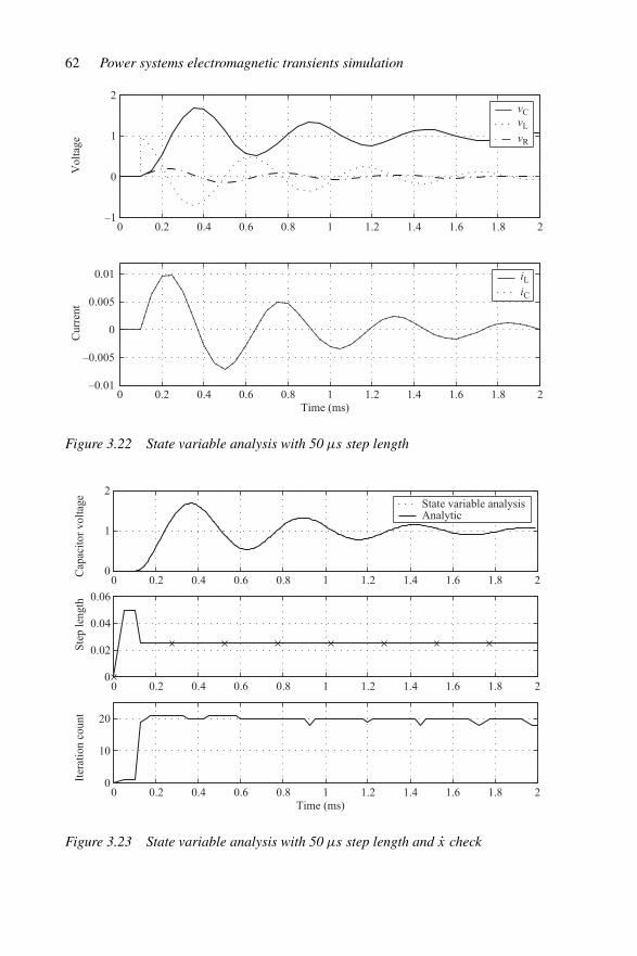
62 Power systems electromagnetic transients simulation
0 0.2 0.4 0.6 0.8 1 1.2 1.4 1.6 1.8 2–1
0
1
2vCvL
vR
0 0.2 0.4 0.6 0.8 1 1.2 1.4 1.6 1.8 2Time (ms)
iLiC
–0.01
–0.005
0
0.005
0.01
Vol
tage
Cur
rent
Figure 3.22 State variable analysis with 50 μs step length
0 0.2 0.4 0.6 0.8 1 1.2 1.4 1.6 1.8 20
1
2State variable analysisAnalytic
0 0.2 0.4 0.6 0.8 1 1.2 1.4 1.6 1.8 20
0.02
0.04
0.06
0 0.2 0.4 0.6 0.8 1 1.2 1.4 1.6 1.8 20
10
20
Time (ms)
Cap
acit
or v
olta
geS
tep
leng
thIt
erat
ion
coun
t
Figure 3.23 State variable analysis with 50 μs step length and x check
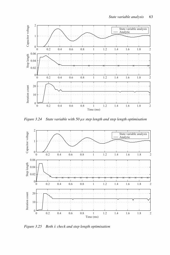
State variable analysis 63
0 0.2 0.4 0.6 0.8 1 1.2 1.4 1.6 1.8 2
State variable analysisAnalytic
0 0.2 0.4 0.6 0.8 1 1.2 1.4 1.6 1.8 2
0 0.2 0.4 0.6 0.8 1 1.2 1.4 1.6 1.8 2Time (ms)
0
1
2
0
0.02
0.04
0.06
0
10
20
Cap
acit
or v
olta
geS
tep
leng
thIt
erat
ion
coun
t
Figure 3.24 State variable with 50 μs step length and step length optimisation
0 0.2 0.4 0.6 0.8 1 1.2 1.4 1.6 1.8 20
1
2State variable analysisAnalytic
0 0.2 0.4 0.6 0.8 1 1.2 1.4 1.6 1.8 20
0.02
0.04
0.06
0 0.2 0.4 0.6 0.8 1 1.2 1.4 1.6 1.8 20
10
20
Time (ms)
Cap
acit
or v
olta
geS
tep
leng
thIt
erat
ion
coun
t
Figure 3.25 Both x check and step length optimisation
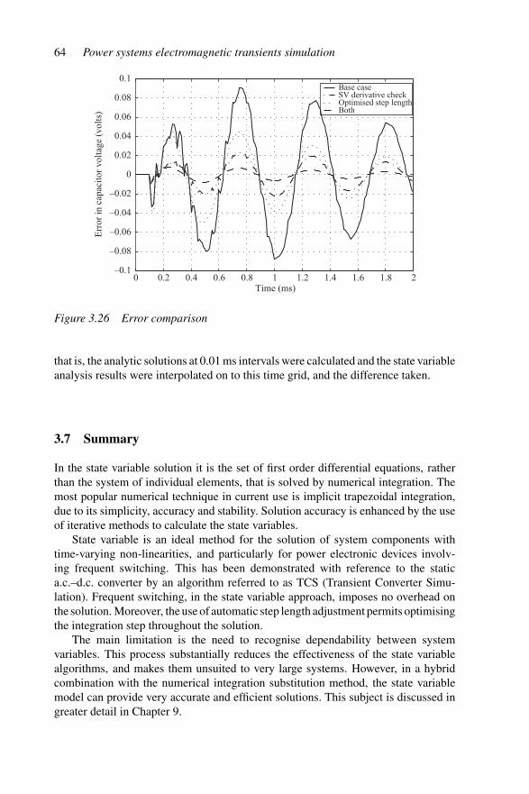
64 Power systems electromagnetic transients simulation
Err
or in
cap
acit
or v
olta
ge (
volt
s)
Time (ms)0 0.2 0.4 0.6 0.8 1 1.2 1.4 1.6 1.8 2
Base caseSV derivative checkOptimised step lengthBoth
–0.1
–0.08
–0.06
–0.04
–0.02
0
0.02
0.04
0.06
0.08
0.1
Figure 3.26 Error comparison
that is, the analytic solutions at 0.01 ms intervals were calculated and the state variableanalysis results were interpolated on to this time grid, and the difference taken.
3.7 Summary
In the state variable solution it is the set of first order differential equations, ratherthan the system of individual elements, that is solved by numerical integration. Themost popular numerical technique in current use is implicit trapezoidal integration,due to its simplicity, accuracy and stability. Solution accuracy is enhanced by the useof iterative methods to calculate the state variables.
State variable is an ideal method for the solution of system components withtime-varying non-linearities, and particularly for power electronic devices involv-ing frequent switching. This has been demonstrated with reference to the statica.c.–d.c. converter by an algorithm referred to as TCS (Transient Converter Simu-lation). Frequent switching, in the state variable approach, imposes no overhead onthe solution. Moreover, the use of automatic step length adjustment permits optimisingthe integration step throughout the solution.
The main limitation is the need to recognise dependability between systemvariables. This process substantially reduces the effectiveness of the state variablealgorithms, and makes them unsuited to very large systems. However, in a hybridcombination with the numerical integration substitution method, the state variablemodel can provide very accurate and efficient solutions. This subject is discussed ingreater detail in Chapter 9.
State variable analysis 65
3.8 References
1 HAY, J. L. and HINGORANI, N. G.: ‘Dynamic simulation of multi-convertorHVdc systems by digital computer’, Proceedings of 6th PICA conference, 1969,pp. 512–35
2 KRON, G.: ‘Diakoptics – the piecewise solution’ (MacDonald, London, 1963)3 CHUA, L. O. and LIN, P. M.: ‘Computer aided analysis of electronic circuits:
algorithms and computational techniques’ (Prentice Hall, Englewood Cliffs, CA,1975)
4 ARRILLAGA, J., AL-KASHALI, H. J. and CAMPOS-BARROS, J. G.: ‘Generalformulation for dynamic studies in power systems including static converters’,Proceedings of IEE, 1977, 124 (11), pp. 1047–52
5 ROHRER, R. A.: ‘Circuit theory, introduction to the state variable approach’(McGraw-Hill, Kogakusha, Tokyo, 1970)
6 JOOSTEN, A. P. B., ARRILLAGA, J., ARNOLD, C. P. and WATSON, N. R.:‘Simulation of HVdc system disturbances with reference to the magnetising his-tory of the convertor transformer’, IEEE Transactions on Power Delivery, 1990,5 (1), pp. 330–6
7 KITCHEN, R. H.: ‘New method for digital-computer evaluation of convertorharmonics in power systems using state-variable analysis’, Proceedings of IEE,Part C, 1981, 128 (4), 196–207
8 RAJAGOPALAN, V.: ‘Computer-aided analysis of power electronic system’(Marcel Dekker, New York, 1987)
9 ARRILLAGA, J., ARNOLD, C. P. and HARKER, B. J.: ‘Computer modelling ofelectrical power systems’ (John Wiley, Chicester, 1983)
10 GEAR, C. W.: ‘Numerical initial value problems in ordinary differentialequations’ (Prentice Hall, Englewood Cliffs, 1971)
11 BOWLES, J. P.: ‘AC system and transformer representation for HV-DC transmis-sion studies’, IEEE Transactions on Power Apparatus and Systems, 1970, 89 (7),pp. 1603–9
12 IEEE Task Force of Harmonics Modeling and Simulation: ‘Test systems for har-monic modeling and simulation’, IEEE Transactions on Power Delivery, 1999,4 (2), pp. 579–87
13 KRUGER, K. H. and LASSETER, R. H.: ‘HVDC simulation using NETOMAC’,Proceedings, IEEE Montec ’86 Conference on HVDC Power Transmission,Sept/Oct 1986, pp. 47–50
14 AINSWORTH, J. D.: ‘The phase-locked oscillator – a new control system for con-trolled static convertors’, IEEE Transactions on Power Apparatus and Systems,1968, 87 (3), pp. 859–65
15 ARRILLAGA, J., SANKAR, S., ARNOLD, C. P. and WATSON, N. R.: ‘Incor-poration of HVdc controller dynamics in transient convertor simulation’, Trans.Inst. Prof. Eng. N.Z. Electrical/Mech/Chem. Engineering Section, 1989, 16 (2),pp. 25–30

Chapter 4
Numerical integrator substitution
4.1 Introduction
A continuous function can be simulated by substituting a numerical integrationformula into the differential equation and rearranging the function into an appropriateform. Among the factors to be taken into account in the selection of the numericalintegrator are the error due to truncated terms, its properties as a differentiator, errorpropagation and frequency response.
Numerical integration substitution (NIS) constitutes the basis of Dommel’s EMTP[1]–[3], which, as explained in the introductory chapter, is now the most generallyaccepted method for the solution of electromagnetic transients. The EMTP methodis an integrated approach to the problems of:
• forming the network differential equations• collecting the equations into a coherent system to be solved• numerical solution of the equations.
The trapezoidal integrator (described in Appendix C) is used for the numericalintegrator substitution, due to its simplicity, stability and reasonable accuracy in mostcircumstances. However, being based on a truncated Taylor’s series, the trapezoidalrule can cause numerical oscillations under certain conditions due to the neglectedterms [4]. This problem will be discussed further in Chapters 5 and 9.
The other basic characteristic of Dommel’s method is the discretisation of thesystem components, given a predetermined time step, which are then combined in asolution for the nodal voltages. Branch elements are represented by the relationshipwhich they maintain between branch current and nodal voltage.
This chapter describes the basic formulation and solution of the numericalintegrator substitution method as implemented in the electromagnetic transientprograms.
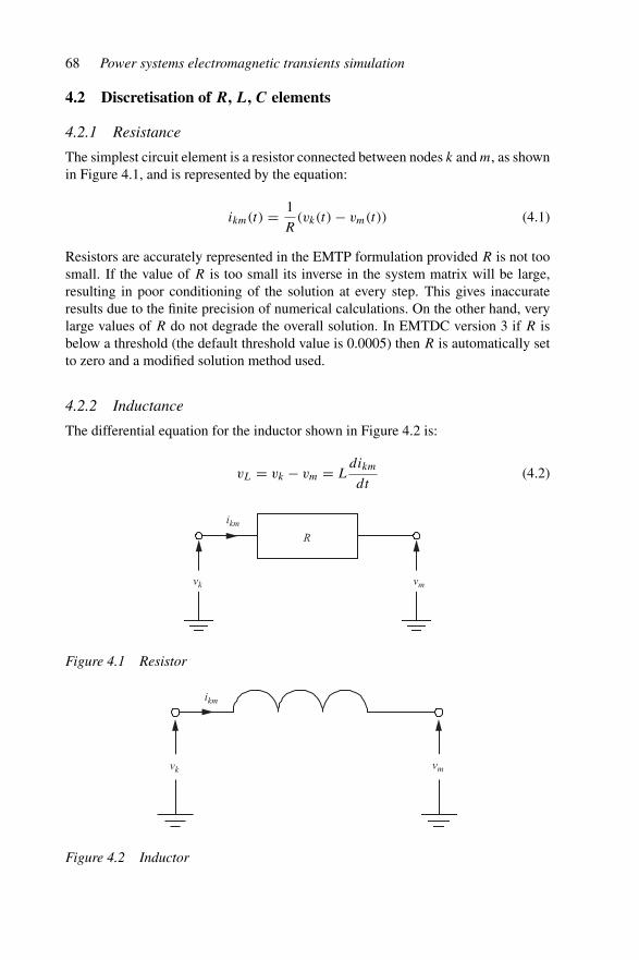
68 Power systems electromagnetic transients simulation
4.2 Discretisation of R, L, C elements
4.2.1 Resistance
The simplest circuit element is a resistor connected between nodes k and m, as shownin Figure 4.1, and is represented by the equation:
ikm(t) = 1
R(vk(t) − vm(t)) (4.1)
Resistors are accurately represented in the EMTP formulation provided R is not toosmall. If the value of R is too small its inverse in the system matrix will be large,resulting in poor conditioning of the solution at every step. This gives inaccurateresults due to the finite precision of numerical calculations. On the other hand, verylarge values of R do not degrade the overall solution. In EMTDC version 3 if R isbelow a threshold (the default threshold value is 0.0005) then R is automatically setto zero and a modified solution method used.
4.2.2 Inductance
The differential equation for the inductor shown in Figure 4.2 is:
vL = vk − vm = Ldikm
dt(4.2)
vk
ikm
R
vm
Figure 4.1 Resistor
vk
ikm
vm
Figure 4.2 Inductor

Numerical integrator substitution 69
Rearranging:
ikm(t) = ikm(t−�t) +∫ t
t−�t
(vk − vm) dt (4.3)
Applying the trapezoidal rule gives:
ikm(t) = ikm(t−�t) + �t
2L((vk − vm)(t) + (vk − vm)(t−�t)) (4.4)
= ikm(t−�t) + �t
2L(vk(t−�t) − vm(t−�t)) + �t
2L(vk(t) − vm(t)) (4.5)
ikm(t) = IHistory(t − �t) + 1
Reff(vk(t) − vm(t)) (4.6)
This equation can be expressed in the form of a Norton equivalent (or companioncircuit) as illustrated in Figure 4.3. The term relating the current contribution at thepresent time step to voltage at the present time step (1/Reff ) is a conductance (instan-taneous term) and the contribution to current from the previous time step quantitiesis a current source (History term).
In equation 4.6 IHistory(t−�t) = ikm(t−�t)+(�t/2L)(vk(t−�t)−vm(t−�t))
and Reff = 2L/�t .The term 2L/�t is known as the instantaneous term as it relates the current to
the voltage at the same time point, i.e. any change in one will instantly be reflectedin the other. As an effective resistance, very small values of L or rather 2L/�t , canalso result in poor conditioning of the conductance matrix.
Transforming equation 4.6 to the z-domain gives:
Ikm(z) = z−1Ikm(z) + �t
2L(1 + z−1)(Vk(z) − Vm(z))
Reff = 2LΔt
k
m
ikm(t)
2L(vk (t − Δt) −vm (t − Δt))
IHistory (t − Δt)Δt= ikm (t − Δt) +
(vk(t) – vm(t))
Figure 4.3 Norton equivalent of the inductor
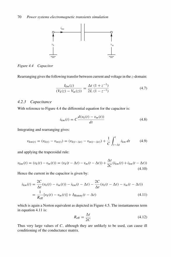
70 Power systems electromagnetic transients simulation
vk
ikm
vm
Figure 4.4 Capacitor
Rearranging gives the following transfer between current and voltage in the z-domain:
Ikm(z)
(Vk(z) − Vm(z))= �t
2L
(1 + z−1)
(1 − z−1)(4.7)
4.2.3 Capacitance
With reference to Figure 4.4 the differential equation for the capacitor is:
ikm(t) = Cd(vk(t) − vm(t))
dt(4.8)
Integrating and rearranging gives:
vkm(t) = (vk(t) − vm(t)) = (vk(t−�t) − vm(t−�t)) + 1
C
∫ t
t−�t
ikm dt (4.9)
and applying the trapezoidal rule:
vkm(t) = (vk(t)− vm(t)) = (vk(t −�t)− vm(t −�t))+ �t
2C(ikm(t)+ ikm(t −�t))
(4.10)Hence the current in the capacitor is given by:
ikm(t) = 2C
�t(vk(t) − vm(t)) − ikm(t − �t) − 2C
�t(vk(t − �t) − vm(t − �t))
= 1
Reff[vk(t) − vm(t)] + IHistory(t − �t) (4.11)
which is again a Norton equivalent as depicted in Figure 4.5. The instantaneous termin equation 4.11 is:
Reff = �t
2C(4.12)
Thus very large values of C, although they are unlikely to be used, can cause illconditioning of the conductance matrix.
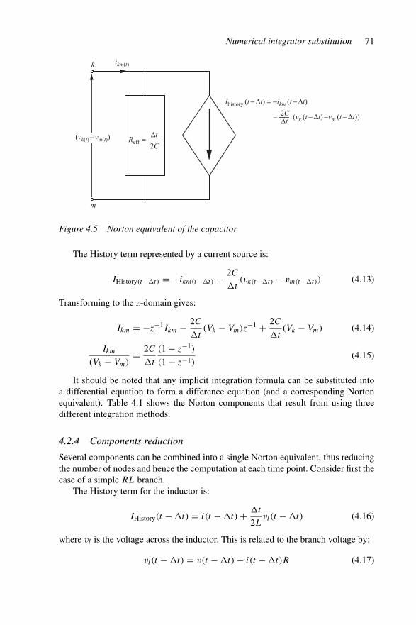
Numerical integrator substitution 71
Reff =2C
Δt
k
m
ikm(t)
2C (vk (t − Δt) −vm (t − Δt))
Ihistory (t − Δt) = −ikm (t − Δt)
Δt
(vk(t) – vm(t))
–
Figure 4.5 Norton equivalent of the capacitor
The History term represented by a current source is:
IHistory(t−�t) = −ikm(t−�t) − 2C
�t(vk(t−�t) − vm(t−�t)) (4.13)
Transforming to the z-domain gives:
Ikm = −z−1Ikm − 2C
�t(Vk − Vm)z−1 + 2C
�t(Vk − Vm) (4.14)
Ikm
(Vk − Vm)= 2C
�t
(1 − z−1)
(1 + z−1)(4.15)
It should be noted that any implicit integration formula can be substituted intoa differential equation to form a difference equation (and a corresponding Nortonequivalent). Table 4.1 shows the Norton components that result from using threedifferent integration methods.
4.2.4 Components reduction
Several components can be combined into a single Norton equivalent, thus reducingthe number of nodes and hence the computation at each time point. Consider first thecase of a simple RL branch.
The History term for the inductor is:
IHistory(t − �t) = i(t − �t) + �t
2Lvl(t − �t) (4.16)
where vl is the voltage across the inductor. This is related to the branch voltage by:
vl(t − �t) = v(t − �t) − i(t − �t)R (4.17)
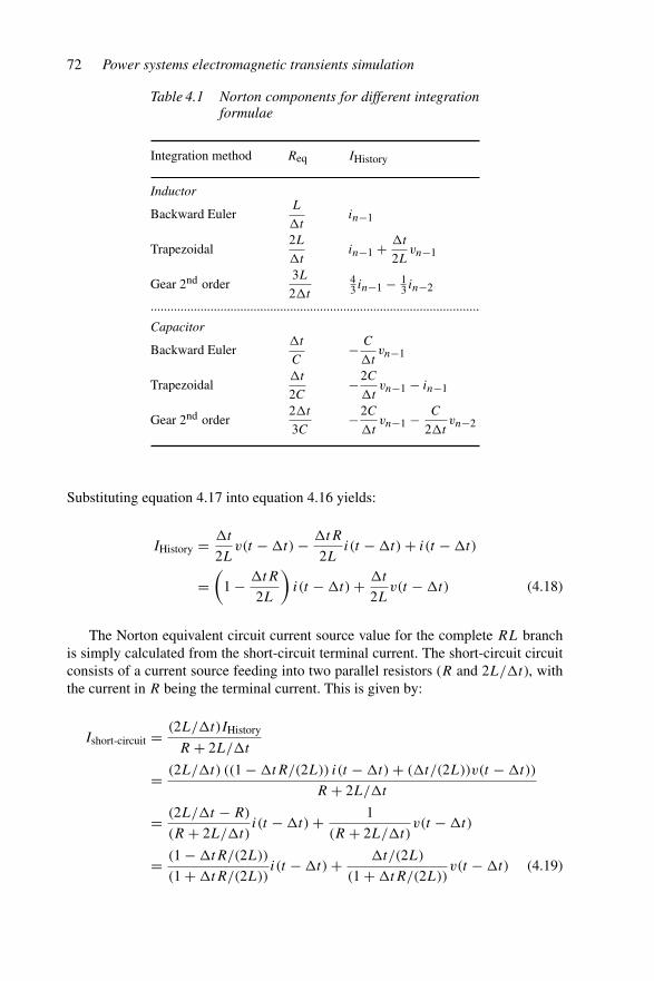
72 Power systems electromagnetic transients simulation
Table 4.1 Norton components for different integrationformulae
Integration method Req IHistory
Inductor
Backward EulerL
�tin−1
Trapezoidal2L
�tin−1 + �t
2Lvn−1
Gear 2nd order3L
2�t43 in−1 − 1
3 in−2
...................................................................................................
Capacitor
Backward Euler�t
C− C
�tvn−1
Trapezoidal�t
2C−2C
�tvn−1 − in−1
Gear 2nd order2�t
3C−2C
�tvn−1 − C
2�tvn−2
Substituting equation 4.17 into equation 4.16 yields:
IHistory = �t
2Lv(t − �t) − �tR
2Li(t − �t) + i(t − �t)
=(
1 − �tR
2L
)i(t − �t) + �t
2Lv(t − �t) (4.18)
The Norton equivalent circuit current source value for the complete RL branchis simply calculated from the short-circuit terminal current. The short-circuit circuitconsists of a current source feeding into two parallel resistors (R and 2L/�t), withthe current in R being the terminal current. This is given by:
Ishort-circuit = (2L/�t)IHistory
R + 2L/�t
= (2L/�t) ((1 − �tR/(2L)) i(t − �t) + (�t/(2L))v(t − �t))
R + 2L/�t
= (2L/�t − R)
(R + 2L/�t)i(t − �t) + 1
(R + 2L/�t)v(t − �t)
= (1 − �tR/(2L))
(1 + �tR/(2L))i(t − �t) + �t/(2L)
(1 + �tR/(2L))v(t − �t) (4.19)
Numerical integrator substitution 73
Reff =Δt2L
2LR
+Δ
t
IRL History =
IL History
2LIL History = ikm (t – Δt) – vL (t – Δt)
Δt
vR (t)
vL (t)
R R
m mm
k k k
(2L / Δt) IL History
R – 2L / Δt
Figure 4.6 Reduction of RL branch
The instantaneous current term is obtained from the current that flows due to anapplied voltage to the terminals (current source open circuited). This current is:
1
(R + 2L/�t)v(t) = �t/(2L)
(1 + �tR/(2L))v(t) (4.20)
Hence the complete difference equation expressed in terms of branch voltage isobtained by adding equations 4.19 and 4.20, which gives:
i(t) = (1 − �tR/(2L))
(1 + �tR/(2L))i(t − �t) + �t/(2L)
(1 + �tR/(2L))(v(t − �t) + v(t)) (4.21)
The corresponding Norton equivalent is shown in Figure 4.6.The reduction of a tuned filter branch is illustrated in Figure 4.7, which shows the
actual RLC components, their individual Norton equivalents and a single Norton rep-resentation of the complete filter branch. Parallel filter branches can be combined intoone Norton by summing their current sources and conductance values. The reduction,however, hides the information on voltages across and current through each individualcomponent. The mathematical implementation of the reduction process is carried outby first establishing the nodal admittance matrix of the circuit and then performingGaussian elimination of the internal nodes.
4.3 Dual Norton model of the transmission line
A detailed description of transmission line modelling is deferred to Chapter 6. Thesingle-phase lossless line [4] is used as an introduction at this stage, to illustrate thesimplicity of Dommel’s method.
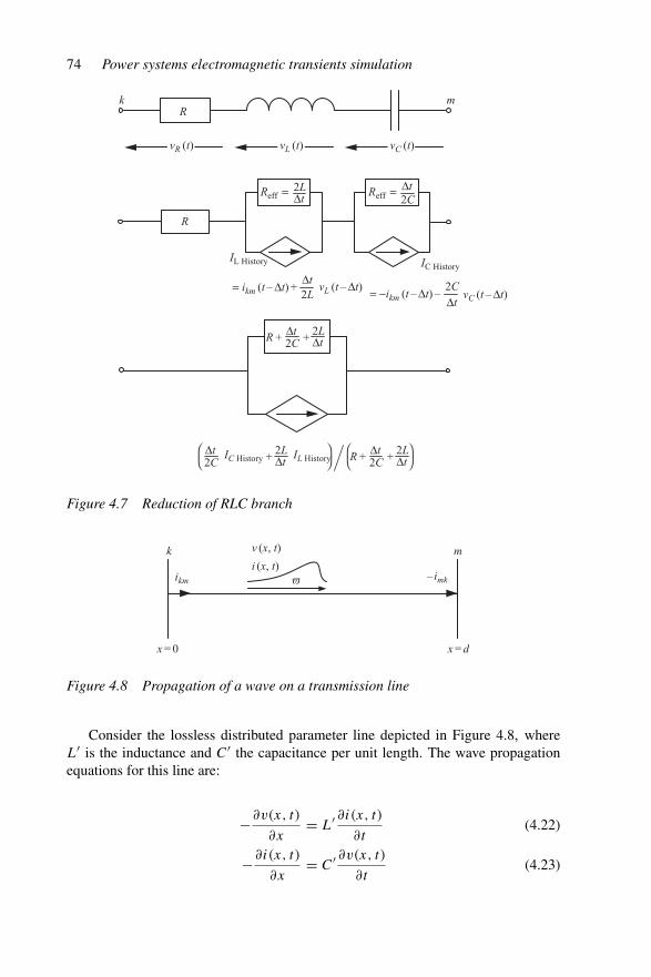
74 Power systems electromagnetic transients simulation
R
R
IC History IL History
2L = ikm (t – Δt) + vL (t – Δt)
Δt2C = −ikm (t – Δt) – vC (t – Δt)Δt
Reff = Δt2L Reff = Δt
2C
vR (t) vL (t) vC (t)
k m
IL History IC History
R + 2CΔt
Δt2L
+
R + 2CΔt
2CΔt
Δt2L
+Δt2L
+
Figure 4.7 Reduction of RLC branch
x = 0 x = d
ikm – imk�
v (x, t)
i (x, t)mk
Figure 4.8 Propagation of a wave on a transmission line
Consider the lossless distributed parameter line depicted in Figure 4.8, whereL′ is the inductance and C′ the capacitance per unit length. The wave propagationequations for this line are:
−∂v(x, t)
∂x= L′ ∂i(x, t)
∂t(4.22)
−∂i(x, t)
∂x= C′ ∂v(x, t)
∂t(4.23)
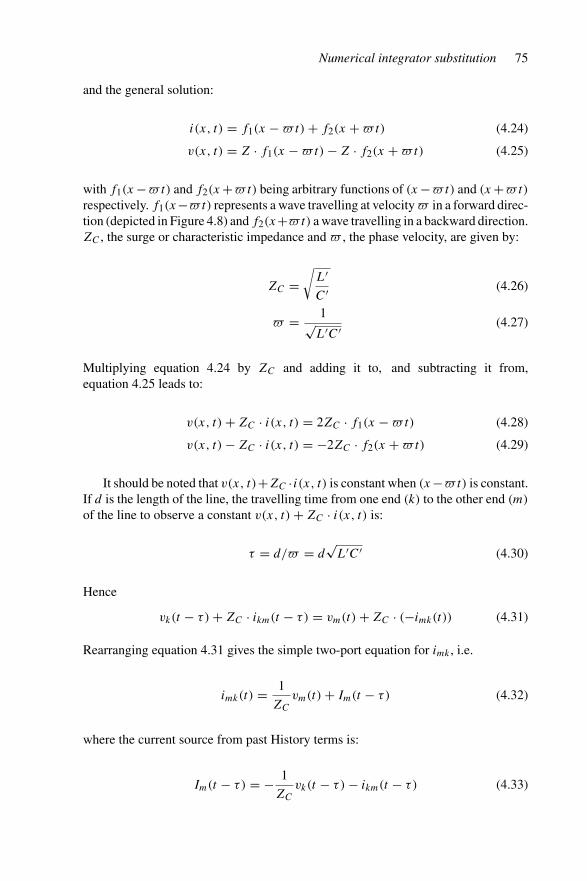
Numerical integrator substitution 75
and the general solution:
i(x, t) = f1(x − �t) + f2(x + �t) (4.24)
v(x, t) = Z · f1(x − �t) − Z · f2(x + �t) (4.25)
with f1(x −�t) and f2(x +�t) being arbitrary functions of (x −�t) and (x +�t)
respectively. f1(x−�t) represents a wave travelling at velocity � in a forward direc-tion (depicted in Figure 4.8) and f2(x+�t) a wave travelling in a backward direction.ZC , the surge or characteristic impedance and � , the phase velocity, are given by:
ZC =√
L′C′ (4.26)
� = 1√L′C′ (4.27)
Multiplying equation 4.24 by ZC and adding it to, and subtracting it from,equation 4.25 leads to:
v(x, t) + ZC · i(x, t) = 2ZC · f1(x − �t) (4.28)
v(x, t) − ZC · i(x, t) = −2ZC · f2(x + �t) (4.29)
It should be noted that v(x, t)+ZC · i(x, t) is constant when (x−�t) is constant.If d is the length of the line, the travelling time from one end (k) to the other end (m)
of the line to observe a constant v(x, t) + ZC · i(x, t) is:
τ = d/� = d√
L′C′ (4.30)
Hence
vk(t − τ) + ZC · ikm(t − τ) = vm(t) + ZC · (−imk(t)) (4.31)
Rearranging equation 4.31 gives the simple two-port equation for imk , i.e.
imk(t) = 1
ZC
vm(t) + Im(t − τ) (4.32)
where the current source from past History terms is:
Im(t − τ) = − 1
ZC
vk(t − τ) − ikm(t − τ) (4.33)
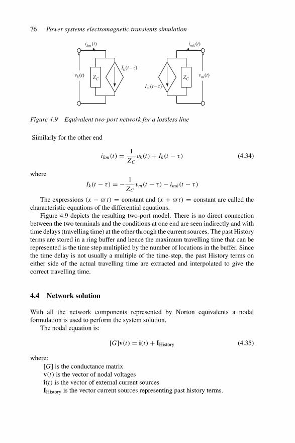
76 Power systems electromagnetic transients simulation
ZC ZCvk (t) vm (t)
ikm (t) imk (t)
Ik (t – �)
Im (t – �)
Figure 4.9 Equivalent two-port network for a lossless line
Similarly for the other end
ikm(t) = 1
ZC
vk(t) + Ik(t − τ) (4.34)
where
Ik(t − τ) = − 1
ZC
vm(t − τ) − imk(t − τ)
The expressions (x − �t) = constant and (x + �t) = constant are called thecharacteristic equations of the differential equations.
Figure 4.9 depicts the resulting two-port model. There is no direct connectionbetween the two terminals and the conditions at one end are seen indirectly and withtime delays (travelling time) at the other through the current sources. The past Historyterms are stored in a ring buffer and hence the maximum travelling time that can berepresented is the time step multiplied by the number of locations in the buffer. Sincethe time delay is not usually a multiple of the time-step, the past History terms oneither side of the actual travelling time are extracted and interpolated to give thecorrect travelling time.
4.4 Network solution
With all the network components represented by Norton equivalents a nodalformulation is used to perform the system solution.
The nodal equation is:
[G]v(t) = i(t) + IHistory (4.35)
where:[G] is the conductance matrixv(t) is the vector of nodal voltagesi(t) is the vector of external current sourcesIHistory is the vector current sources representing past history terms.
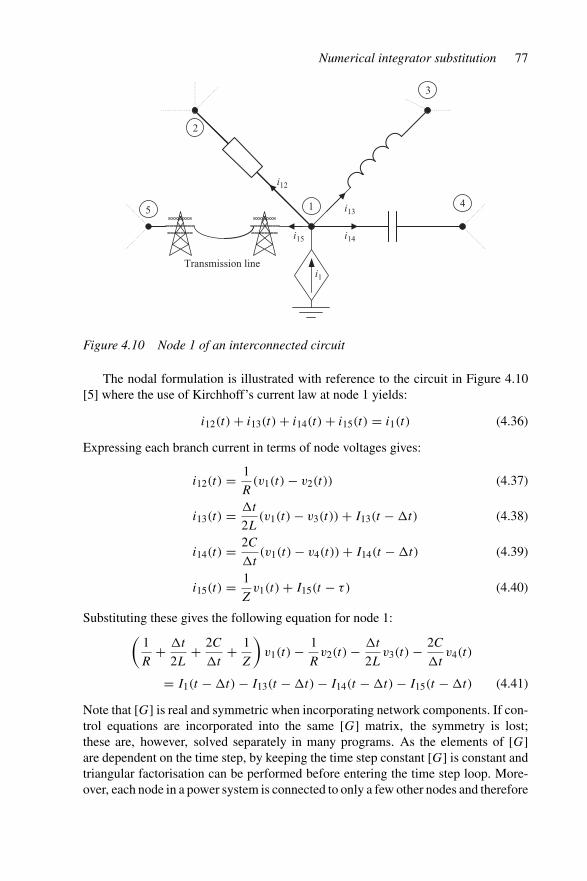
Numerical integrator substitution 77
i12
i13
i14i15
i1Transmission line
5
2
3
41
Figure 4.10 Node 1 of an interconnected circuit
The nodal formulation is illustrated with reference to the circuit in Figure 4.10[5] where the use of Kirchhoff’s current law at node 1 yields:
i12(t) + i13(t) + i14(t) + i15(t) = i1(t) (4.36)
Expressing each branch current in terms of node voltages gives:
i12(t) = 1
R(v1(t) − v2(t)) (4.37)
i13(t) = �t
2L(v1(t) − v3(t)) + I13(t − �t) (4.38)
i14(t) = 2C
�t(v1(t) − v4(t)) + I14(t − �t) (4.39)
i15(t) = 1
Zv1(t) + I15(t − τ) (4.40)
Substituting these gives the following equation for node 1:(
1
R+ �t
2L+ 2C
�t+ 1
Z
)v1(t) − 1
Rv2(t) − �t
2Lv3(t) − 2C
�tv4(t)
= I1(t − �t) − I13(t − �t) − I14(t − �t) − I15(t − �t) (4.41)
Note that [G] is real and symmetric when incorporating network components. If con-trol equations are incorporated into the same [G] matrix, the symmetry is lost;these are, however, solved separately in many programs. As the elements of [G]are dependent on the time step, by keeping the time step constant [G] is constant andtriangular factorisation can be performed before entering the time step loop. More-over, each node in a power system is connected to only a few other nodes and therefore
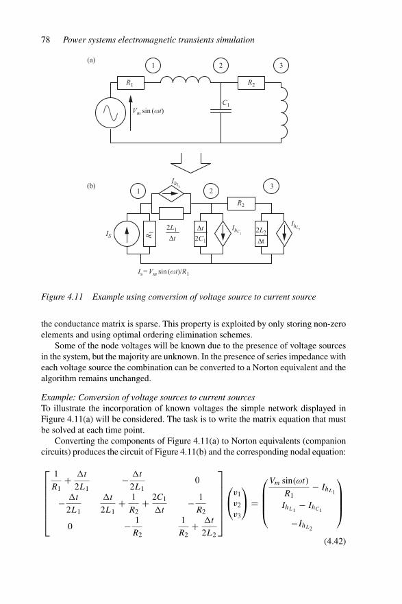
78 Power systems electromagnetic transients simulation
2C1
Δt
Δt
2L1
Is = Vm sin (�t)/R1
ISΔt
2L2
IhL1
IhL2IhC
1
R1
R1
R2
R2
C1Vm sin (�t)
1
1
2
2
3
3
(a)
(b)
Figure 4.11 Example using conversion of voltage source to current source
the conductance matrix is sparse. This property is exploited by only storing non-zeroelements and using optimal ordering elimination schemes.
Some of the node voltages will be known due to the presence of voltage sourcesin the system, but the majority are unknown. In the presence of series impedance witheach voltage source the combination can be converted to a Norton equivalent and thealgorithm remains unchanged.
Example: Conversion of voltage sources to current sourcesTo illustrate the incorporation of known voltages the simple network displayed inFigure 4.11(a) will be considered. The task is to write the matrix equation that mustbe solved at each time point.
Converting the components of Figure 4.11(a) to Norton equivalents (companioncircuits) produces the circuit of Figure 4.11(b) and the corresponding nodal equation:
⎡
⎢⎢⎢⎢⎢⎢⎣
1
R1+ �t
2L1− �t
2L10
− �t
2L1
�t
2L1+ 1
R2+ 2C1
�t− 1
R2
0 − 1
R2
1
R2+ �t
2L2
⎤
⎥⎥⎥⎥⎥⎥⎦
⎛
⎝v1v2v3
⎞
⎠ =
⎛
⎜⎜⎜⎝
Vm sin(ωt)
R1− IhL1
IhL1− IhC1
−IhL2
⎞
⎟⎟⎟⎠
(4.42)
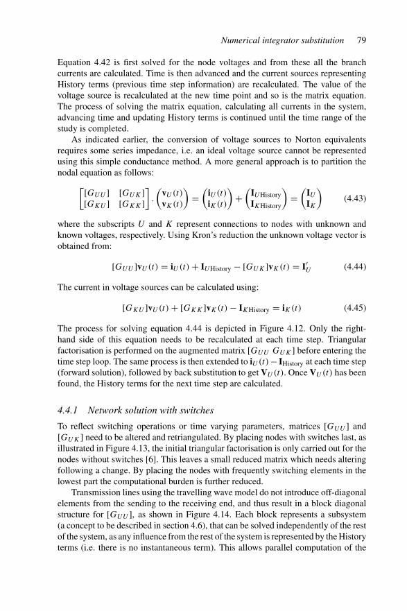
Numerical integrator substitution 79
Equation 4.42 is first solved for the node voltages and from these all the branchcurrents are calculated. Time is then advanced and the current sources representingHistory terms (previous time step information) are recalculated. The value of thevoltage source is recalculated at the new time point and so is the matrix equation.The process of solving the matrix equation, calculating all currents in the system,advancing time and updating History terms is continued until the time range of thestudy is completed.
As indicated earlier, the conversion of voltage sources to Norton equivalentsrequires some series impedance, i.e. an ideal voltage source cannot be representedusing this simple conductance method. A more general approach is to partition thenodal equation as follows:
[[GUU ] [GUK ][GKU ] [GKK ]
].
(vU(t)
vK(t)
)=
(iU(t)
iK(t)
)+
(IUHistoryIKHistory
)=
(IU
IK
)(4.43)
where the subscripts U and K represent connections to nodes with unknown andknown voltages, respectively. Using Kron’s reduction the unknown voltage vector isobtained from:
[GUU ]vU(t) = iU(t) + IUHistory − [GUK ]vK(t) = I′U (4.44)
The current in voltage sources can be calculated using:
[GKU ]vU(t) + [GKK ]vK(t) − IKHistory = iK(t) (4.45)
The process for solving equation 4.44 is depicted in Figure 4.12. Only the right-hand side of this equation needs to be recalculated at each time step. Triangularfactorisation is performed on the augmented matrix [GUU GUK ] before entering thetime step loop. The same process is then extended to iU(t)− IHistory at each time step(forward solution), followed by back substitution to get VU(t). Once VU(t) has beenfound, the History terms for the next time step are calculated.
4.4.1 Network solution with switches
To reflect switching operations or time varying parameters, matrices [GUU ] and[GUK ] need to be altered and retriangulated. By placing nodes with switches last, asillustrated in Figure 4.13, the initial triangular factorisation is only carried out for thenodes without switches [6]. This leaves a small reduced matrix which needs alteringfollowing a change. By placing the nodes with frequently switching elements in thelowest part the computational burden is further reduced.
Transmission lines using the travelling wave model do not introduce off-diagonalelements from the sending to the receiving end, and thus result in a block diagonalstructure for [GUU ], as shown in Figure 4.14. Each block represents a subsystem(a concept to be described in section 4.6), that can be solved independently of the restof the system, as any influence from the rest of the system is represented by the Historyterms (i.e. there is no instantaneous term). This allows parallel computation of the
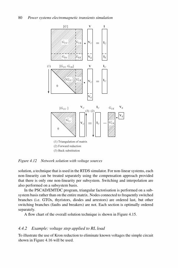
80 Power systems electromagnetic transients simulation
=
GUU
[GUU GUK]
[GUU ]
0
0
–
[G ]
•
•
(1)
'UUG
•
GUK
GUK
GBA GKK
V
VU
I
VK
VK
VK
VK
VU
VU
VU
V
IK
IU
IU
IU
IU
IU
G�UU G�UK
G�UK
(3) (2)
=
=
(1) Triangulation of matrix
(2) Forward reduction
(3) Back substitution
Figure 4.12 Network solution with voltage sources
solution, a technique that is used in the RTDS simulator. For non-linear systems, eachnon-linearity can be treated separately using the compensation approach providedthat there is only one non-linearity per subsystem. Switching and interpolation arealso performed on a subsystem basis.
In the PSCAD/EMTDC program, triangular factorisation is performed on a sub-system basis rather than on the entire matrix. Nodes connected to frequently switchedbranches (i.e. GTOs, thyristors, diodes and arrestors) are ordered last, but otherswitching branches (faults and breakers) are not. Each section is optimally orderedseparately.
A flow chart of the overall solution technique is shown in Figure 4.15.
4.4.2 Example: voltage step applied to RL load
To illustrate the use of Kron reduction to eliminate known voltages the simple circuitshown in Figure 4.16 will be used.
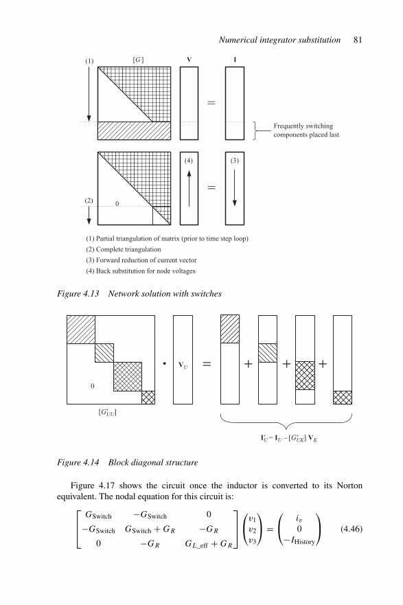
Numerical integrator substitution 81
[G ] V I
0
Frequently switching components placed last
=
=
(1) Partial triangulation of matrix (prior to time step loop)
(2) Complete triangulation
(3) Forward reduction of current vector
(4) Back substitution for node voltages
(1)
(2)
(3)(4)
Figure 4.13 Network solution with switches
VU
[G�UU]
I�U = IU – [G�UK] VK
0
• = + + +
Figure 4.14 Block diagonal structure
Figure 4.17 shows the circuit once the inductor is converted to its Nortonequivalent. The nodal equation for this circuit is:
⎡
⎢⎣
GSwitch −GSwitch 0
−GSwitch GSwitch + GR −GR
0 −GR GL_eff + GR
⎤
⎥⎦
⎛
⎝v1v2v3
⎞
⎠ =⎛
⎝iv0
−IHistory
⎞
⎠ (4.46)
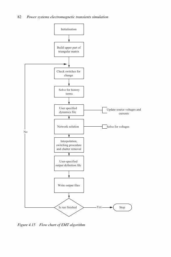
82 Power systems electromagnetic transients simulation
Initialisation
Build upper part of triangular matrix
Is run finished
Check switches for change
Solve for history terms
User specified dynamics file
Network solution
User-specifiedoutput definition file
Interpolation,switching procedure and chatter removal
Write output files
Yes Stop
No
Solve for voltages
Update source voltages andcurrents
Figure 4.15 Flow chart of EMT algorithm

Numerical integrator substitution 83
ivR = 100 Ω
L = 50 mH
1 2
3
R
Figure 4.16 Simple switched RL load
1 2
3
RSwitch
Riv
RL eff
Figure 4.17 Equivalent circuit for simple switched RL load
As v1 is a known voltage the conductance matrix is reordered by placing v1 last inthe column vector of nodal voltages and moving column 1 of [G] to be column 3;then move row 1 (equation for current in voltage source) to become row 3. This thengives:
⎡
⎣GSwitch + GR −GR
−GR GL_eff + GR
−GSwitch0
−GSwitch 0 GSwitch
⎤
⎦
⎛
⎝v2v3
v1
⎞
⎠ =⎛
⎝0
−IHistory
iv
⎞
⎠ (4.47)
which is of the form[[GUU ] [GUK ][GKU ] [GKK ]
](vU(t)
vK(t)
)=
(iU(t)
iK(t)
)+
(IU_HistoryIK_History
)
i.e.[GSwitch + GR −GR −GSwitch
−GR GL_eff + GR 0
]⎛
⎝v2v3v1
⎞
⎠ =(
0−IHistory
)
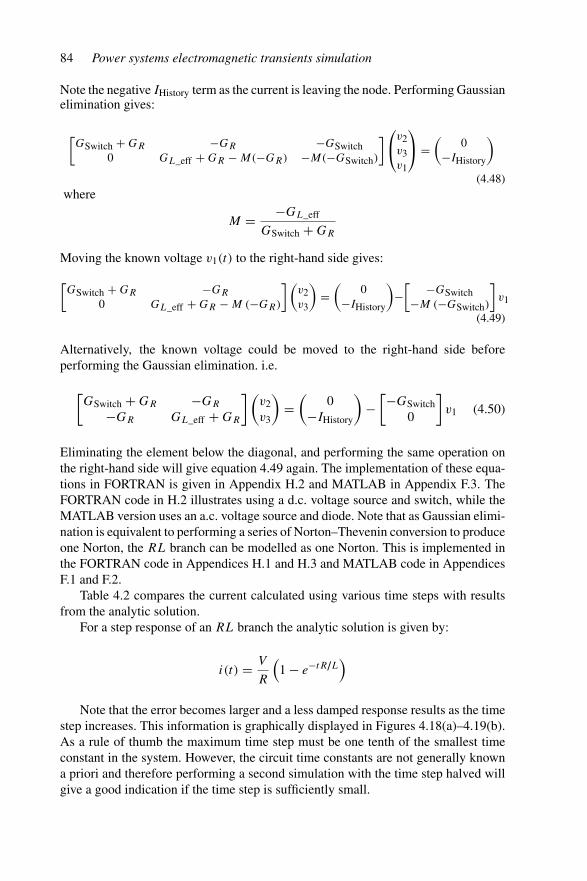
84 Power systems electromagnetic transients simulation
Note the negative IHistory term as the current is leaving the node. Performing Gaussianelimination gives:
[GSwitch + GR −GR −GSwitch
0 GL_eff + GR − M(−GR) −M(−GSwitch)
]⎛
⎝v2v3v1
⎞
⎠ =(
0−IHistory
)
(4.48)where
M = −GL_eff
GSwitch + GR
Moving the known voltage v1(t) to the right-hand side gives:
[GSwitch + GR −GR
0 GL_eff + GR − M (−GR)
](v2v3
)=
(0
−IHistory
)−[ −GSwitch−M (−GSwitch)
]v1
(4.49)
Alternatively, the known voltage could be moved to the right-hand side beforeperforming the Gaussian elimination. i.e.
[GSwitch + GR −GR
−GR GL_eff + GR
](v2v3
)=
(0
−IHistory
)−
[−GSwitch0
]v1 (4.50)
Eliminating the element below the diagonal, and performing the same operation onthe right-hand side will give equation 4.49 again. The implementation of these equa-tions in FORTRAN is given in Appendix H.2 and MATLAB in Appendix F.3. TheFORTRAN code in H.2 illustrates using a d.c. voltage source and switch, while theMATLAB version uses an a.c. voltage source and diode. Note that as Gaussian elimi-nation is equivalent to performing a series of Norton–Thevenin conversion to produceone Norton, the RL branch can be modelled as one Norton. This is implemented inthe FORTRAN code in Appendices H.1 and H.3 and MATLAB code in AppendicesF.1 and F.2.
Table 4.2 compares the current calculated using various time steps with resultsfrom the analytic solution.
For a step response of an RL branch the analytic solution is given by:
i(t) = V
R
(1 − e−tR/L
)
Note that the error becomes larger and a less damped response results as the timestep increases. This information is graphically displayed in Figures 4.18(a)–4.19(b).As a rule of thumb the maximum time step must be one tenth of the smallest timeconstant in the system. However, the circuit time constants are not generally knowna priori and therefore performing a second simulation with the time step halved willgive a good indication if the time step is sufficiently small.

Numerical integrator substitution 85
Table 4.2 Step response of RL circuit to various step lengths
Time (ms) Current (amps)
Exact �t = τ/10 �t = τ �t = 5τ �t = 10τ
1.0000 0 0 0 0 01.0500 63.2121 61.3082 33.3333 – –1.1000 86.4665 85.7779 77.7778 – –1.1500 95.0213 94.7724 92.5926 – –1.2000 98.1684 98.0785 97.5309 – –1.2500 99.3262 99.2937 99.1770 71.4286 –1.3000 99.7521 99.7404 99.7257 – –1.3500 99.9088 99.9046 99.9086 – –1.4000 99.9665 99.9649 99.9695 – –1.4500 99.9877 99.9871 99.9898 – –1.5000 99.9955 99.9953 99.9966 112.2449 83.33331.5500 99.9983 99.9983 99.9989 – –1.6000 99.9994 99.9994 99.9996 – –1.6500 99.9998 99.9998 99.9999 – –1.7000 99.9999 99.9999 100.0000 – –1.7500 100.0000 100.0000 100.0000 94.7522 –1.8000 100.0000 100.0000 100.0000 – –1.8500 100.0000 100.0000 100.0000 – –1.9000 100.0000 100.0000 100.0000 – –1.9500 100.0000 100.0000 100.0000 – –2.0000 100.0000 100.0000 100.0000 102.2491 111.11112.0500 100.0000 100.0000 100.0000 – –2.1000 100.0000 100.0000 100.0000 – –2.1500 100.0000 100.0000 100.0000 – –2.2000 100.0000 100.0000 100.0000 – –2.2500 100.0000 100.0000 100.0000 99.0361 –2.3000 100.0000 100.0000 100.0000 – –2.3500 100.0000 100.0000 100.0000 – –2.4000 100.0000 100.0000 100.0000 – –2.4500 100.0000 100.0000 100.0000 – –2.5000 100.0000 100.0000 100.0000 100.4131 92.59262.5500 100.0000 100.0000 100.0000 – –2.6000 100.0000 100.0000 100.0000 – –2.6500 100.0000 100.0000 100.0000 – –2.7000 100.0000 100.0000 100.0000 – –2.7500 100.0000 100.0000 100.0000 99.8230 –2.8000 100.0000 100.0000 100.0000 – –2.8500 100.0000 100.0000 100.0000 – –2.9000 100.0000 100.0000 100.0000 – –2.9500 100.0000 100.0000 100.0000 – –3.0000 100.0000 100.0000 100.0000 100.0759 104.9383
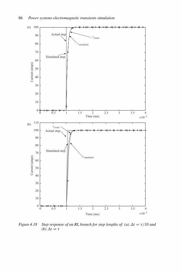
86 Power systems electromagnetic transients simulation
0 0.5 1 1.5 2 2.5 3 3.5 4
×10–3
×10–3
Time (ms)
Actual step
Simulated step
i simulated
i exact
0
10
20
30
40
50
60
70
80
90
100
0 0.5 1 1.5 2 2.5 3 3.5 4
Time (ms)
Actual step
Simulated step
i simulated
i exact
0
10
20
30
40
50
60
70
80
90
100
110
Cur
rent
(am
ps)
Cur
rent
(am
ps)
(a)
(b)
Figure 4.18 Step response of an RL branch for step lengths of: (a) Δt = τ/10 and(b) Δt = τ
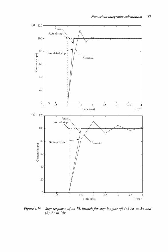
Numerical integrator substitution 87
× 10–3
× 10–3
Cur
rent
(am
ps)
Time (ms)
Actual step
Simulated stepi simulated
i exact
0
20
40
60
80
100
120
0 0.5 1 1.5 2 2.5 3 3.5 4
0 0.5 1 1.5 2 2.5 3 3.5 4
Cur
rent
(am
ps)
Time (ms)
Actual step
Simulated step i simulated
i exact
0
20
40
60
80
100
120
(a)
(b)
Figure 4.19 Step response of an RL branch for step lengths of: (a) Δt = 5τ and(b) Δt = 10τ

88 Power systems electromagnetic transients simulation
The following data is used for this test system: �t = 50 μs, R = 1.0 �,L = 0.05 mH and RSwitch = 1010 � (OFF) 10−10 � (ON) and V1 = 100 V.
Initially IHistory = 0
[1.000000000 −1.000000000 −.1000000000E−09
−1.000000000 1.500000000 0.000000000
]⎛
⎝v2v3v1
⎞
⎠ =(
0.0000000000.000000000
)
The multiplier is −0.999999999900000. After forward reduction using this multiplierthe G matrix becomes:
[1.000000000 −1.000000000 −.1000000000E−090.000000000 0.5000000001 −.9999999999E−10
]⎛
⎝v2v3v1
⎞
⎠ =(
0.0000000000.000000000
)
Moving the known voltage v1 to the right-hand side gives[
1.000000000 −1.0000000000.000000000 0.5000000001
](v2v3
)=
(0.0000000000.000000000
)−
[−.1000000000E−09−.9999999999E−10
]v1
Back substitution gives: i = 9.9999999970E−009 or essentially zero in the offstate. When the switch is closed the G matrix is updated and the equation becomes:
[0.1000000000E+11 −1.000000000 −.1000000000E+11
−1.000000000 1.500000000 0.000000000
]⎛
⎝v2v3v1
⎞
⎠ =(
0.0000000000.000000000
)
After forward reduction:
[0.1000000000E+11 −1.000000000 −.1000000000E+11
−1.000000000 1.500000000 −.9999999999
]⎛
⎝v2v3v1
⎞
⎠ =(
0.0000000000.000000000
)
Moving the known voltage v1 to the right-hand side gives[
1.000000000 −1.0000000000.000000000 1.500000000
](v2v3
)=
(0.0000000000.000000000
)−
[−.1000000000E+11−.9999999999
]v1
=(
0.1000000000E+1399.99999999
)
Hence back-substitution gives:
iL = 33.333 A
v2 = 66.667 V
v3 = 33.333 V
4.5 Non-linear or time varying parameters
The most common types of non-linear elements that need representing are induc-tances under magnetic saturation for transformers and reactors and resistances of
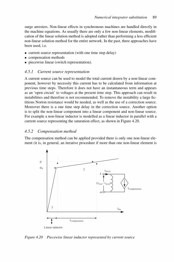
Numerical integrator substitution 89
surge arresters. Non-linear effects in synchronous machines are handled directly inthe machine equations. As usually there are only a few non-linear elements, modifi-cation of the linear solution method is adopted rather than performing a less efficientnon-linear solution method for the entire network. In the past, three approaches havebeen used, i.e.
• current source representation (with one time step delay)• compensation methods• piecewise linear (switch representation).
4.5.1 Current source representation
A current source can be used to model the total current drawn by a non-linear com-ponent, however by necessity this current has to be calculated from information atprevious time steps. Therefore it does not have an instantaneous term and appearsas an ‘open circuit’ to voltages at the present time step. This approach can result ininstabilities and therefore is not recommended. To remove the instability a large fic-titious Norton resistance would be needed, as well as the use of a correction source.Moreover there is a one time step delay in the correction source. Another optionis to split the non-linear component into a linear component and non-linear source.For example a non-linear inductor is modelled as a linear inductor in parallel with acurrent source representing the saturation effect, as shown in Figure 4.20.
4.5.2 Compensation method
The compensation method can be applied provided there is only one non-linear ele-ment (it is, in general, an iterative procedure if more than one non-linear element is
ikm
iCompensation
ikm (t)
iCompensation
(vk (t) – vm (t))
m
k
�0
�
Linear inductor
3
2
Figure 4.20 Piecewise linear inductor represented by current source
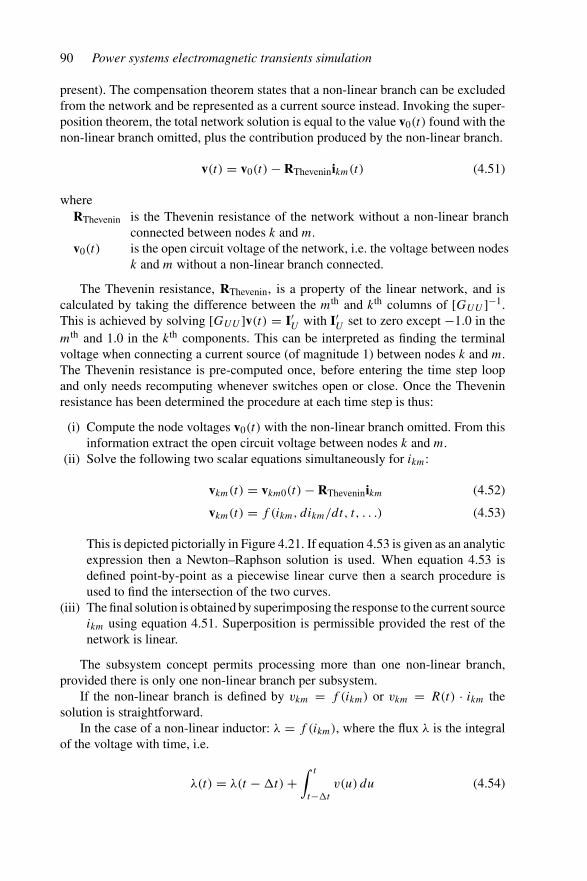
90 Power systems electromagnetic transients simulation
present). The compensation theorem states that a non-linear branch can be excludedfrom the network and be represented as a current source instead. Invoking the super-position theorem, the total network solution is equal to the value v0(t) found with thenon-linear branch omitted, plus the contribution produced by the non-linear branch.
v(t) = v0(t) − RTheveninikm(t) (4.51)
whereRThevenin is the Thevenin resistance of the network without a non-linear branch
connected between nodes k and m.v0(t) is the open circuit voltage of the network, i.e. the voltage between nodes
k and m without a non-linear branch connected.
The Thevenin resistance, RThevenin, is a property of the linear network, and iscalculated by taking the difference between the mth and kth columns of [GUU ]−1.This is achieved by solving [GUU ]v(t) = I′
U with I′U set to zero except −1.0 in the
mth and 1.0 in the kth components. This can be interpreted as finding the terminalvoltage when connecting a current source (of magnitude 1) between nodes k and m.The Thevenin resistance is pre-computed once, before entering the time step loopand only needs recomputing whenever switches open or close. Once the Theveninresistance has been determined the procedure at each time step is thus:
(i) Compute the node voltages v0(t) with the non-linear branch omitted. From thisinformation extract the open circuit voltage between nodes k and m.
(ii) Solve the following two scalar equations simultaneously for ikm:
vkm(t) = vkm0(t) − RTheveninikm (4.52)
vkm(t) = f (ikm, dikm/dt, t, . . .) (4.53)
This is depicted pictorially in Figure 4.21. If equation 4.53 is given as an analyticexpression then a Newton–Raphson solution is used. When equation 4.53 isdefined point-by-point as a piecewise linear curve then a search procedure isused to find the intersection of the two curves.
(iii) The final solution is obtained by superimposing the response to the current sourceikm using equation 4.51. Superposition is permissible provided the rest of thenetwork is linear.
The subsystem concept permits processing more than one non-linear branch,provided there is only one non-linear branch per subsystem.
If the non-linear branch is defined by vkm = f (ikm) or vkm = R(t) · ikm thesolution is straightforward.
In the case of a non-linear inductor: λ = f (ikm), where the flux λ is the integralof the voltage with time, i.e.
λ(t) = λ(t − �t) +∫ t
t−�t
v(u) du (4.54)

Numerical integrator substitution 91
vkm (t ) = f (t,ikm,dikm /dt,)
vkm (t ) = vkm0 (t ) RThevenin ikm
vkm
ikm
Figure 4.21 Pictorial view of simultaneous solution of two equations
The use of the trapezoidal rule gives:
λ(t) = �t
2v(t) + λHistory(t − �t) (4.55)
where
λHistory = λ(t − �t) + �t
2v(t − �)
Numerical problems can occur with non-linear elements if �t is too large. Thenon-linear characteristics are effectively sampled and the characteristics between thesampled points do not enter the solution. This can result in artificial negative dampingor hysteresis as depicted in Figure 4.22.
4.5.3 Piecewise linear method
The piecewise linear inductor characteristic, depicted in Figure 4.23, can be repre-sented as a linear inductor in series with a voltage source. The inductance is changed(switched) when moving from one segment of the characteristic to the next. Althoughthis model is easily implemented, numerical problems can occur as the need to changeto the next segment is only recognised after the point exceeds the current segment(unless interpolation is used for this type of discontinuity). This is a switched modelin that when the segment changes the branch conductance changes, hence the systemconductance matrix must be modified.
A non-linear function can be modelled using a combination of piecewise lin-ear representation and current source. The piecewise linear characteristics can bemodelled with switched representation, and a current source used to correct for thedifference between the piecewise linear characteristic and the actual.
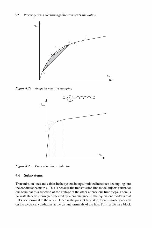
92 Power systems electromagnetic transients simulation
vkm
ikm
1
2
3
Figure 4.22 Artificial negative damping
�km
ikm
k m
Figure 4.23 Piecewise linear inductor
4.6 Subsystems
Transmission lines and cables in the system being simulated introduce decoupling intothe conductance matrix. This is because the transmission line model injects current atone terminal as a function of the voltage at the other at previous time steps. There isno instantaneous term (represented by a conductance in the equivalent models) thatlinks one terminal to the other. Hence in the present time step, there is no dependencyon the electrical conditions at the distant terminals of the line. This results in a block
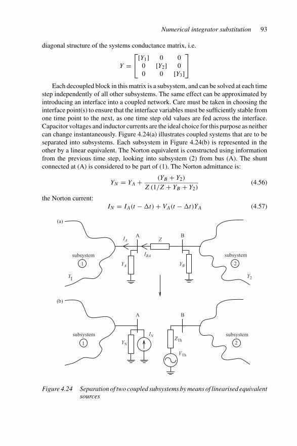
Numerical integrator substitution 93
diagonal structure of the systems conductance matrix, i.e.
Y =⎡
⎣[Y1] 0 0
0 [Y2] 00 0 [Y3]
⎤
⎦
Each decoupled block in this matrix is a subsystem, and can be solved at each timestep independently of all other subsystems. The same effect can be approximated byintroducing an interface into a coupled network. Care must be taken in choosing theinterface point(s) to ensure that the interface variables must be sufficiently stable fromone time point to the next, as one time step old values are fed across the interface.Capacitor voltages and inductor currents are the ideal choice for this purpose as neithercan change instantaneously. Figure 4.24(a) illustrates coupled systems that are to beseparated into subsystems. Each subsystem in Figure 4.24(b) is represented in theother by a linear equivalent. The Norton equivalent is constructed using informationfrom the previous time step, looking into subsystem (2) from bus (A). The shuntconnected at (A) is considered to be part of (1). The Norton admittance is:
YN = YA + (YB + Y2)
Z (1/Z + YB + Y2)(4.56)
the Norton current:IN = IA(t − �t) + VA(t − �t)YA (4.57)
IA
IBA
YA YB
Y2Y1
1
subsystem
2
subsystem
1
subsystem
2
subsystemZTh
IN
YN
VTh
A B
A B
Z
(a)
(b)
Figure 4.24 Separation of two coupled subsystems by means of linearised equivalentsources
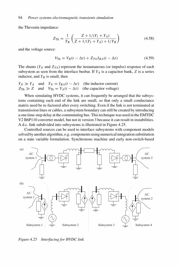
94 Power systems electromagnetic transients simulation
the Thevenin impedance:
ZTh = 1
YB
(Z + 1/(Y1 + YA)
Z + 1/(Y1 + YA) + 1/YB
)(4.58)
and the voltage source:
VTh = VB(t − �t) + ZT hIBA(t − �t) (4.59)
The shunts (YN and ZT h) represent the instantaneous (or impulse) response of eachsubsystem as seen from the interface busbar. If YA is a capacitor bank, Z is a seriesinductor, and YB is small, then
YN YA and YN = IBA(t − �t) (the inductor current)ZTh Z and VTh = VA(t − �t) (the capacitor voltage)
When simulating HVDC systems, it can frequently be arranged that the subsys-tems containing each end of the link are small, so that only a small conductancematrix need be re-factored after every switching. Even if the link is not terminated attransmission lines or cables, a subsystem boundary can still be created by introducinga one time-step delay at the commutating bus. This technique was used in the EMTDCV2 B6P110 converter model, but not in version 3 because it can result in instabilities.A d.c. link subdivided into subsystems is illustrated in Figure 4.25.
Controlled sources can be used to interface subsystems with component modelssolved by another algorithm, e.g. components using numerical integration substitutionon a state variable formulation. Synchronous machine and early non-switch-based
Subsystem 1 Subsystem 2 Subsystem 3 Subsystem 4
ACsystem 2
ACsystem 2
ACsystem 1
ACsystem 1
(a)
(b)
Figure 4.25 Interfacing for HVDC link
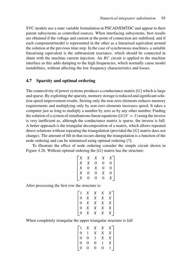
Numerical integrator substitution 95
SVC models use a state variable formulation in PSCAD/EMTDC and appear to theirparent subsystems as controlled sources. When interfacing subsystems, best resultsare obtained if the voltage and current at the point of connection are stabilised, and ifeach component/model is represented in the other as a linearised equivalent aroundthe solution at the previous time step. In the case of synchronous machines, a suitablelinearising equivalent is the subtransient reactance, which should be connected inshunt with the machine current injection. An RC circuit is applied to the machineinterface as this adds damping to the high frequencies, which normally cause modelinstabilities, without affecting the low frequency characteristics and losses.
4.7 Sparsity and optimal ordering
The connectivity of power systems produces a conductance matrix [G] which is largeand sparse. By exploiting the sparsity, memory storage is reduced and significant solu-tion speed improvement results. Storing only the non-zero elements reduces memoryrequirements and multiplying only by non-zero elements increases speed. It takes acomputer just as long to multiply a number by zero as by any other number. Findingthe solution of a system of simultaneous linear equations ([G]V = I ) using the inverseis very inefficient as, although the conductance matrix is sparse, the inverse is full.A better approach is the triangular decomposition of a matrix, which allows repeateddirect solutions without repeating the triangulation (provided the [G] matrix does notchange). The amount of fill-in that occurs during the triangulation is a function of thenode ordering and can be minimised using optimal ordering [7].
To illustrate the effect of node ordering consider the simple circuit shown inFigure 4.26. Without optimal ordering the [G] matrix has the structure:
⎡
⎢⎢⎢⎢⎣
X X X X X
X X 0 0 0X 0 X 0 0X 0 0 X 0X 0 0 0 X
⎤
⎥⎥⎥⎥⎦
After processing the first row the structure is:⎡
⎢⎢⎢⎢⎣
1 X X X X
0 X X X X
0 X X X X
0 X X X X
0 X X X X
⎤
⎥⎥⎥⎥⎦
When completely triangular the upper triangular structure is full⎡
⎢⎢⎢⎢⎣
1 X X X X
0 1 X X X
0 0 1 X X
0 0 0 1 X
0 0 0 0 1
⎤
⎥⎥⎥⎥⎦
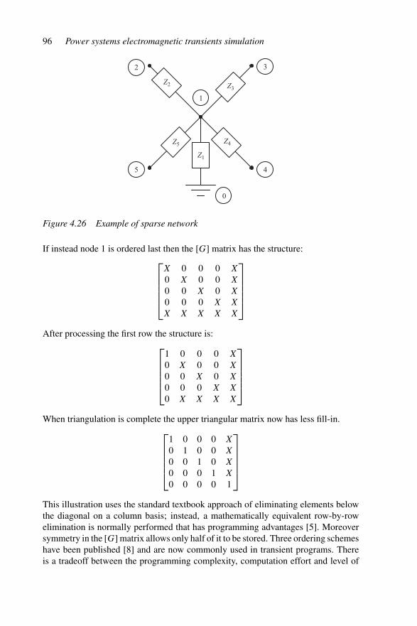
96 Power systems electromagnetic transients simulation
Z2 Z3
Z4
Z1
Z5
2
5 4
3
1
0
Figure 4.26 Example of sparse network
If instead node 1 is ordered last then the [G] matrix has the structure:⎡
⎢⎢⎢⎢⎣
X 0 0 0 X
0 X 0 0 X
0 0 X 0 X
0 0 0 X X
X X X X X
⎤
⎥⎥⎥⎥⎦
After processing the first row the structure is:⎡
⎢⎢⎢⎢⎣
1 0 0 0 X
0 X 0 0 X
0 0 X 0 X
0 0 0 X X
0 X X X X
⎤
⎥⎥⎥⎥⎦
When triangulation is complete the upper triangular matrix now has less fill-in.⎡
⎢⎢⎢⎢⎣
1 0 0 0 X
0 1 0 0 X
0 0 1 0 X
0 0 0 1 X
0 0 0 0 1
⎤
⎥⎥⎥⎥⎦
This illustration uses the standard textbook approach of eliminating elements belowthe diagonal on a column basis; instead, a mathematically equivalent row-by-rowelimination is normally performed that has programming advantages [5]. Moreoversymmetry in the [G] matrix allows only half of it to be stored. Three ordering schemeshave been published [8] and are now commonly used in transient programs. Thereis a tradeoff between the programming complexity, computation effort and level of
Numerical integrator substitution 97
optimality achieved by these methods, and the best scheme depends on the networktopology, size and number of direct solutions required.
4.8 Numerical errors and instabilities
The trapezoidal rule contains a truncation error which normally manifests itself aschatter or simply as an error in the waveforms when the time step is large. This isparticularly true if cutsets of inductors and current sources, or loops of capacitorsand voltage sources exist. Whenever discontinuities occur (switching of devices, ormodification of non-linear component parameters, …) care is needed as these caninitiate chatter problems or instabilities. Two separate problems are associated withdiscontinuities. The first is the error in making changes at the next time point after thediscontinuity, for example current chopping in inductive circuits due to turning OFFa device at the next time point after the current has gone to zero, or proceeding on asegment of a piecewise linear characteristic one step beyond the knee point. Even ifthe discontinuity is not stepped over, chatter can occur due to error in the trapezoidalrule. These issues, as they apply to power electronic circuits, are dealt with further inChapter 9.
Other instabilities can occur because of time step delays inherent in the model.For example this could be due to an interface between a synchronous machine modeland the main algorithm, or from feedback paths in control systems (Chapter 8).Instabilities can also occur in modelling non-linear devices due to the sampled natureof the simulation as outlined in section 4.5. Finally ‘bang–bang’ instability can occurdue to the interaction of power electronic device non-linearity and non-linear devicessuch as surge arresters. In this case the state of one influences the other and findingthe appropriate state can be difficult.
4.9 Summary
The main features making numerical integration substitution a popular method forthe solution of electromagnetic transients are: simplicity, general applicability andcomputing efficiency.
Its simplicity derives from the conversion of the individual power system ele-ments (i.e. resistance, inductance and capacitance) and the transmission lines intoNorton equivalents easily solvable by nodal analysis. The Norton current source rep-resents the component past History terms and the Norton impedance consists of apure conductance dependent on the step length.
By selecting the appropriate integration step, numerical integration substitutionis applicable to all transient phenomena and to systems of any size. In some cases,however, the inherent truncation error of the trapezoidal method may lead to oscilla-tions; improved numerical techniques to overcome this problem will be discussed inChapters 5 and 9.
Efficient solutions are possible by the use of a constant integration step lengththroughout the study, which permits performing a single conductance matrix
98 Power systems electromagnetic transients simulation
triangular factorisation before entering the time step loop. Further efficiency isachieved by exploiting the large sparsity of the conductance matrix.
An important concept is the use of subsystems, each of which, at a given timestep, can be solved independently of the others. The main advantage of subsystemsis the performance improvement when multiple time-steps/interpolation algorithmsare used. Interpolating back to discontinuities is performed only on one subsystem.Subsystems also allow parallel processing hence real-time applications as well asinterfacing different solution algorithms. If sparsity techniques are not used (earlyEMTDC versions) then subsystems also greatly improve the performance.
4.10 References
1 DOMMEL, H. W.: ‘Digital computer solution of electromagnetic transients insingle- and multi-phase networks’, IEEE Transactions on Power Apparatus andSystems, 1969, 88 (2), pp. 734–41
2 DOMMEL, H. W.: ‘Nonlinear and time-varying elements in digital simulation ofelectromagnetic transients’, IEEE Transactions on Power Apparatus and Systems,1971, 90 (6), pp. 2561–7
3 DOMMEL, H. W.: ‘Techniques for analyzing electromagnetic transients’, IEEEComputer Applications in Power, 1997, 10 (3), pp. 18–21
4 BRANIN, F. H.: ‘Computer methods of network analysis’, Proceedings of IEEE,1967, 55, pp. 1787–1801
5 DOMMEL, H. W.: ‘Electromagnetic transients program reference manual: EMTPtheory book’ (Bonneville Power Administration, Portland, OR, August 1986).
6 DOMMEL, H. W.: ‘A method for solving transient phenomena in multiphasesystems’, Proc. 2nd Power System Computation Conference, Stockholm, 1966,Rept. 5.8
7 SATO, N. and TINNEY, W. F.: ‘Techniques for exploiting the sparsity of the net-work admittance matrix’, Transactions on Power Apparatus and Systems, 1963,82, pp. 944–50
8 TINNEY, W. F. and WALKER, J. W.: ‘Direct solutions of sparse network equationsby optimally ordered triangular factorization’, Proceedings of IEEE, 1967, 55,pp. 1801–9

Chapter 5
The root-matching method
5.1 Introduction
The integration methods based on a truncated Taylor’s series are prone to numericaloscillations when simulating step responses.
An interesting alternative to numerical integration substitution that has alreadyproved its effectiveness in the control area, is the exponential form of the differ-ence equation. The implementation of this method requires the use of root-matchingtechniques and is better known by that name.
The purpose of the root-matching method is to transfer correctly the poles andzeros from the s-plane to the z-plane, an important requirement for reliable digitalsimulation, to ensure that the difference equation is suitable to simulate the continuousprocess correctly.
This chapter describes the use of root-matching techniques in electromagnetictransient simulation and compares its performance with that of the conventionalnumerical integrator substitution method described in Chapter 4.
5.2 Exponential form of the difference equation
The application of the numerical integrator substitution method, and the trapezoidalrule, to a series RL branch produces the following difference equation for the branch:
ik = (1 − �tR/(2L))
(1 + �tR/(2L))ik−1 + �t/(2L)
(1 + �tR/(2L))(vk + vk−1) (5.1)
Careful inspection of equation 5.1 shows that the first term is a first order approx-imation of e−x , where x = �tR/L and the second term is a first order approximationof (1 − e−x)/2 [1]. This suggests that the use of the exponential expressions in thedifference equation should eliminate the truncation error and thus provide accurateand stable solutions regardless of the time step.
100 Power systems electromagnetic transients simulation
Equation 5.1 can be expressed as:
ik = e−�tR/Lik−1 +(
1 − e−�tR/L)
vk (5.2)
Although the exponential form of the difference equation can be deduced from thedifference equation developed by the numerical integrator substitution method, thisapproach is unsuitable for most transfer functions or electrical circuits, due to thedifficulty in identifying the form of the exponential that has been truncated. Theroot-matching technique provides a rigorous method.
Numerical integrator substitution provides a mapping from continuous to discretetime, or equivalently from the s to the z-domain. The integration rule used will influ-ence the mapping and hence the error. Table 5.1 shows the characteristics of forwardrectangular, backward rectangular (implicit or backward Euler) and trapezoidal inte-grators, including the mapping of poles in the left-hand half s-plane into the z-plane.If the continuous system is stable (has all its poles in the left-hand half s-plane) thenunder forward Euler the poles in the z-plane can lie outside the unit circle and hencean unstable discrete system can result. Both backward Euler and the trapezoidal rulegive stable discrete systems, however stability gives no indication of the accuracy ofthe representation.
The use of the trapezoidal integrator is equivalent to the bilinear transform (orTustin method) for transforming from a continuous to a discrete system, the formerbeing the time representation of the latter. To illustrate this point the bilinear transformwill be next derived from the trapezoidal rule.
In the s-plane the expression for integration is:
Y (s)
X(s)= 1
s(5.3)
In discrete time the trapezoidal rule is expressed as:
yn = yn−1 + �t
2(xn + xn−1) (5.4)
Transforming equation 5.4 to the z-plane gives:
Y (z) = z−1Y (z) + �t
2(X(z) + X(z)z−1) (5.5)
Rearranging gives for integration in the z-domain:
Y (z)
X(z)= �t
2
(1 + z−1)
(1 − z−1)(5.6)
Equating the two integration expressions (i.e. equations 5.3 and 5.6) gives the wellknown bilinear transform equation:
s ≈ 2
�t
(1 − z−1)
(1 + z−1)(5.7)
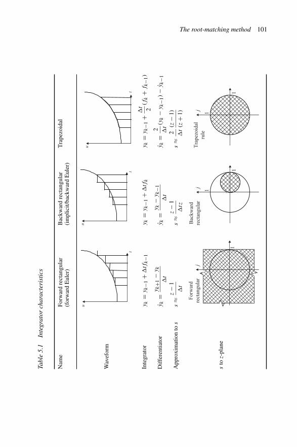
The root-matching method 101
Tabl
e5.
1In
tegr
ator
char
acte
rist
ics
Nam
eFo
rwar
dre
ctan
gula
rB
ackw
ard
rect
angu
lar
Tra
pezo
idal
(for
war
dE
uler
)(i
mpl
icit/
back
war
dE
uler
)
Wav
efor
m
u
tt
uu
t
Inte
grat
oryk
=yk−1
+�
tfk−1
yk
=yk−1
+�
tfk
yk
=yk−1
+�
t 2(f
k+
fk−1
)
Dif
fere
ntia
tor
yk
=yk+1
−yk
�t
yk
=yk
−yk−1
�t
yk
=2 �t(y
k−
yk−1
)−
yk−1
App
roxi
mat
ion
tos
s≈
z−
1
�t
s≈
z−
1
�tz
s≈
2 �t
(z−
1)
(z+
1)
sto
z-p
lane
jF
orw
ard
rect
angu
lar
1
jB
ackw
ard
rect
angu
lar
1
1
jT
rape
zoid
alru
le
1
1

102 Power systems electromagnetic transients simulation
Hence the trapezoidal rule and the bilinear transform give the same mapping betweenthe s and z-planes and are therefore identical.
Equation 5.7 can also be derived from an approximation of an exponential. Theactual relationship between s and z is:
z = es�t (5.8)
Hencez−1 = e−s�t (5.9)
Expressing e−s�t as two exponential functions and then using the series approxima-tion gives:
z−1 = e−s�t = e−s�t/2
es�t/2≈ (1 − s�t/2)
(1 + s�t/2)(5.10)
Rearranging for s gives:
s ≈ 2
�t· (1 − z−1)
(1 + z−1)(5.11)
which is identical to equation 5.7. Hence the trapezoidal rule (and many other inte-gration rules for that matter) can be considered as a truncated series approximationof the exact relationship between s and z.
5.3 z-domain representation of difference equations
Digital simulation requires the use of the z-domain, either in the form of a transferfunction or as an equivalent difference equation.
In the transfer function approach:
H(z) = a0 + a1 · z−1 + a2 · z−2 + · · · + am · z−m
1 + b1 · z−1 + b2 · z−2 + · · · + bm · z−m= Y (z)
U(z)(5.12)
or expressed as a two-sided recursion [2]
(a0 + a1 · z−1 + a2 · z−2 + · · · + am · z−m
)U(z)
=(
1 + b1 · z−1 + b2 · z−2 + · · · + bm · z−m)
Y (z) (5.13)
Equation 5.13 can be implemented directly and without any approximation as a Nortonequivalent.
Rearranging equation 5.13 gives:
Y (z) =(a0 + a1 · z−1 + a2 · z−2 + · · · + am · z−m
)U(z)
−(b1 · z−1 + b2 · z−2 + · · · + bm · z−m
)Y (z) (5.14)
The root-matching method 103
The corresponding difference equation is:
y(k�t) = (a0 · u + a1 · u−1 + a2 · u−2 + · · · + am · u−m)
− (b1 · y−1 + b2 · y−2 + · · · + bm · y−m) (5.15)
The first term on the right side of equation 5.15 is the instantaneous term betweeninput and output, while the other terms are history terms. Hence the conductance isa0 and the history term is:
a1u−1 + a2u−2 + · · · + amu−m − b1y−1 + b2y−2 + · · · + bmy−m (5.16)
Whereas in the s-domain stability is ensured if poles are in the left-hand half-plane,the equivalent criterion in the z-plane is that the poles must reside inside the unitcircle.
In the transformation from the s to z-plane, as required by digital simulation, thepoles and zeros must be transformed correctly and this is the purpose of the root-matching technique. In other words, to ensure that a difference equation is suitableto simulate a continuous process the poles, zeros and final value of the differenceequation should match those of the actual system. If these conditions are met thedifference equations are intrinsically stable, provided the actual system is stable,regardless of the step size. The difference equations generated by this method involveexponential functions, as the transform equation z−1 = e−s�t is used rather thansome approximation to it.
When integrator substitution is used to derive a difference equation, the polesand zeros usually are not inspected, and these can therefore be poorly positioned orthere can even be extra poles and zeros. Because the poles and zeros of the differenceequation do not match well those of the continuous system, there are situations whenthe difference equation is a poor representation of the continuous system.
The steps followed in the application of the root-matching technique are:
1. Determine the transfer function in the s-plane, H(s) and the position of its polesand zeros.
2. Write the transfer function H(s) in the z-plane using the mapping z = es�t , thusensuring the poles and zeros are in the correct place. Also add a constant to allowadjustment of the final value.
3. Use the final value theorem to compute the final value of H(s) for a unit step input.4. Determine the final value of H(z) for unit step input and adjust the constant to be
the correct value.5. Add extra zeros depending on the assumed input variation between solution points.6. Write the resulting z-domain equation in the form of a difference equation.
The final value of H(s) must not be zero to allow the final value matching constantin H(z) to be determined. When that happens the final value is matched for a differentinput. For example some systems respond to the derivative of the input and in suchcases the final value for a unit ramp input is used.
Appendix E (sections E.1 and E.2) illustrate the use of the above procedure witha single order lag function and a first order differential pole, respectively. Table 5.2
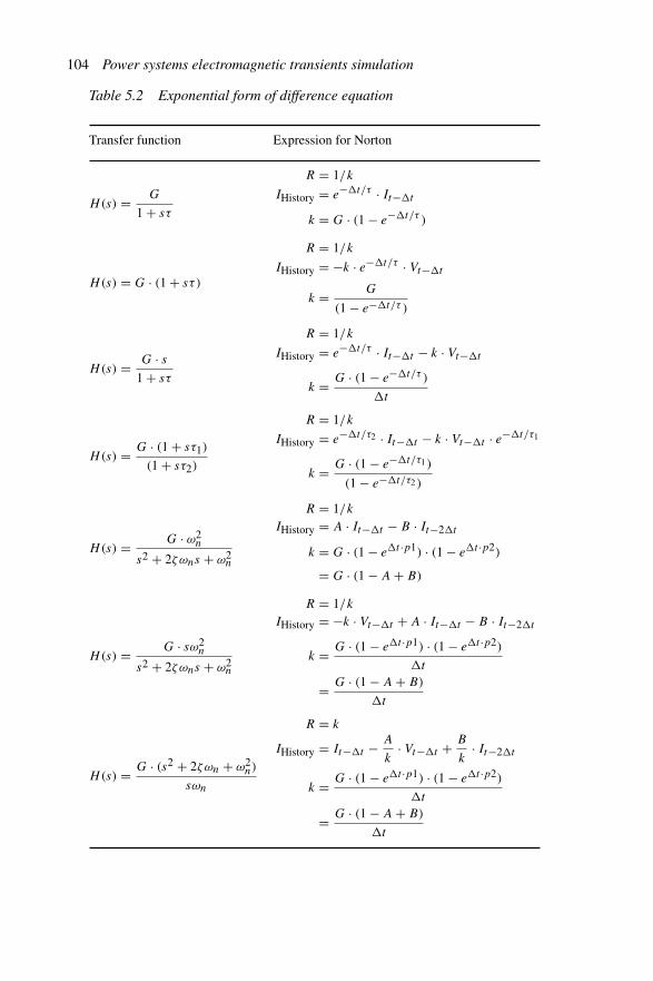
104 Power systems electromagnetic transients simulation
Table 5.2 Exponential form of difference equation
Transfer function Expression for Norton
H(s) = G
1 + sτ
R = 1/k
IHistory = e−�t/τ · It−�t
k = G · (1 − e−�t/τ )
H(s) = G · (1 + sτ )
R = 1/k
IHistory = −k · e−�t/τ · Vt−�t
k = G
(1 − e−�t/τ )
H(s) = G · s
1 + sτ
R = 1/k
IHistory = e−�t/τ · It−�t − k · Vt−�t
k = G · (1 − e−�t/τ )
�t
H(s) = G · (1 + sτ1)
(1 + sτ2)
R = 1/k
IHistory = e−�t/τ2 · It−�t − k · Vt−�t · e−�t/τ1
k = G · (1 − e−�t/τ1)
(1 − e−�t/τ2 )
H(s) = G · ω2n
s2 + 2ζωns + ω2n
R = 1/k
IHistory = A · It−�t − B · It−2�t
k = G · (1 − e�t ·p1) · (1 − e�t ·p2)
= G · (1 − A + B)
H(s) = G · sω2n
s2 + 2ζωns + ω2n
R = 1/k
IHistory = −k · Vt−�t + A · It−�t − B · It−2�t
k = G · (1 − e�t ·p1) · (1 − e�t ·p2)
�t
= G · (1 − A + B)
�t
H(s) = G · (s2 + 2ζωn + ω2n)
sωn
R = k
IHistory = It−�t − A
k· Vt−�t + B
k· It−2�t
k = G · (1 − e�t ·p1) · (1 − e�t ·p2)
�t
= G · (1 − A + B)
�t
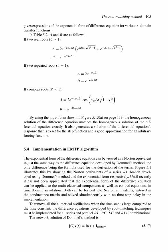
The root-matching method 105
gives expressions of the exponential form of difference equation for various s-domaintransfer functions.
In Table 5.2, A and B are as follows:If two real roots (ζ > 1):
A = 2e−ζωn�t(e�tωn
√ζ 2−1 + e−�tωn
√ζ 2−1
)
B = e−2ζωn�t
If two repeated roots (ζ = 1):
A = 2e−ωn�t
B = e−2ωn�t
If complex roots (ζ < 1):
A = 2e−ζωn�t cos
(ωn�t
√1 − ζ 2
)
B = e−2ζωn�t
By using the input form shown in Figure 5.13(a) on page 113, the homogeneoussolution of the difference equation matches the homogeneous solution of the dif-ferential equation exactly. It also generates a solution of the differential equation’sresponse that is exact for the step function and a good approximation for an arbitraryforcing function.
5.4 Implementation in EMTP algorithm
The exponential form of the difference equation can be viewed as a Norton equivalentin just the same way as the difference equation developed by Dommel’s method, theonly difference being the formula used for the derivation of the terms. Figure 5.1illustrates this by showing the Norton equivalents of a series RL branch devel-oped using Dommel’s method and the exponential form respectively. Until recentlyit has not been appreciated that the exponential form of the difference equationcan be applied to the main electrical components as well as control equations, intime domain simulation. Both can be formed into Norton equivalents, entered inthe conductance matrix and solved simultaneously with no time step delay in theimplementation.
To remove all the numerical oscillations when the time step is large compared tothe time constant, the difference equations developed by root-matching techniquesmust be implemented for all series and parallel RL, RC, LC and RLC combinations.
The network solution of Dommel’s method is:
[G]v(t) = i(t) + IHistory (5.17)

106 Power systems electromagnetic transients simulation
2LR +
Δt
IHistory =
IHistory IHistory
ikm (t) ikm (t)
vkm (t)
i(t – Δt) + v (t – Δt) IHistory= e– ΔtR / L i (t – Δt)
mm
k k
Dommel’s method Exponential form
R(1−e– ΔtR / L)
(1− ΔtR / (2L))
(1+ ΔtR / (2L)) (1+ ΔtR / (2L))
(Δt / (2L))
Figure 5.1 Norton equivalent for RL branch
Structurally the root-matching algorithm is the same as Dommel’s, the only differ-ence being in the formula used for the derivation of the conductance and past historyterms. Moreover, although the root-matching technique can also be applied to singleL or C elements, there is no need for that, as in such cases the response is no longerof an exponential form. Hence Dommel’s algorithm is still used for converting indi-vidual L and C elements to a Norton equivalent. This allows difference equations,hence Norton equivalents, based on root-matching methods to be used in existingelectromagnetic transient programs easily, yet giving unparalleled improvement inaccuracy, particularly for large time steps.
In the new algorithm, IHistory includes the history terms of both Dommel’s and theroot-matching method. Similarly the conductance matrix, which contains the conduc-tance terms of the Norton equivalents, includes some terms from Dommel’s techniqueand others of the exponential form developed from the root-matching technique.
The main characteristics of the exponential form that permit an efficientimplementation are:
• The exponential term is calculated and stored prior to entering the time step loop.• During the time step loop only two multiplications and one addition are required
to calculate the IHistory term. It is thus more efficient than NIS using thetrapezoidal rule.
• Fewer previous time step variables are required. Only the previous time step currentis needed for an RL circuit, while Dommel’s method requires both current andvoltage at the previous time-step.
Three simple test cases are used to illustrate the algorithm’s capability [3]. Thefirst case shown in Figure 5.2 relates to the switching of a series RL branch. Usinga �t = τ time step (τ being the time constant of the circuit), Figure 5.3 showsthe current response derived from Dommel’s method, the exponential method and
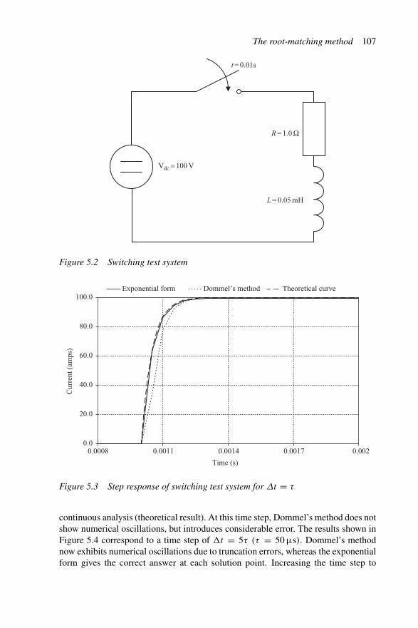
The root-matching method 107
Vdc = 100 V
t = 0.01s
R = 1.0 Ω
L = 0.05 mH
Figure 5.2 Switching test system
Cur
rent
(am
ps)
0.0008 0.0011 0.0014 0.0017 0.002
Time (s)
Exponential form Dommel’s method Theoretical curve
40.0
60.0
80.0
100.0
0.0
20.0
Figure 5.3 Step response of switching test system for Δt = τ
continuous analysis (theoretical result). At this time step, Dommel’s method does notshow numerical oscillations, but introduces considerable error. The results shown inFigure 5.4 correspond to a time step of �t = 5τ (τ = 50 μs). Dommel’s methodnow exhibits numerical oscillations due to truncation errors, whereas the exponentialform gives the correct answer at each solution point. Increasing the time step to
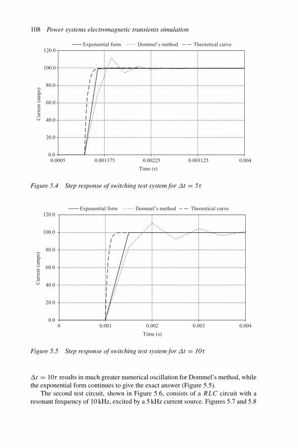
108 Power systems electromagnetic transients simulation
0.0
20.0
40.0
60.0
80.0
100.0
120.0
Cur
rent
(am
ps)
Time (s)
Exponential form Dommel’s method Theoretical curve
0.0005 0.001375 0.00225 0.003125 0.004
Figure 5.4 Step response of switching test system for Δt = 5τ
Cur
rent
(am
ps)
Time (s)
Exponential form Dommel’s method Theoretical curve
0.0
20.0
40.0
60.0
80.0
100.0
120.0
0 0.001 0.002 0.003 0.004
Figure 5.5 Step response of switching test system for Δt = 10τ
�t = 10τ results in much greater numerical oscillation for Dommel’s method, whilethe exponential form continues to give the exact answer (Figure 5.5).
The second test circuit, shown in Figure 5.6, consists of a RLC circuit with aresonant frequency of 10 kHz, excited by a 5 kHz current source. Figures 5.7 and 5.8
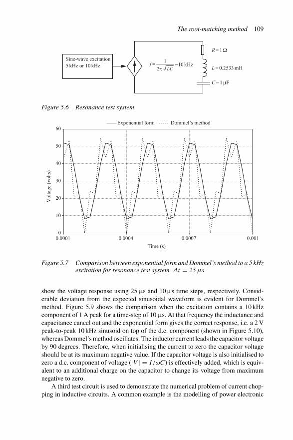
The root-matching method 109
Sine-wave excitation 5 kHz or 10 kHz
LCf =
2π1
L = 0.2533 mH
R = 1 Ω
C = 1 μF
=10 kHz
Figure 5.6 Resonance test system
Vol
tage
(vo
lts)
0.0001 0.0004 0.0007 0.001
Time (s)
Exponential form Dommel’s method
0
10
20
30
40
50
60
Figure 5.7 Comparison between exponential form and Dommel’s method to a 5 kHzexcitation for resonance test system. Δt = 25 μs
show the voltage response using 25 μs and 10 μs time steps, respectively. Consid-erable deviation from the expected sinusoidal waveform is evident for Dommel’smethod. Figure 5.9 shows the comparison when the excitation contains a 10 kHzcomponent of 1 A peak for a time-step of 10 μs. At that frequency the inductance andcapacitance cancel out and the exponential form gives the correct response, i.e. a 2 Vpeak-to-peak 10 kHz sinusoid on top of the d.c. component (shown in Figure 5.10),whereas Dommel’s method oscillates. The inductor current leads the capacitor voltageby 90 degrees. Therefore, when initialising the current to zero the capacitor voltageshould be at its maximum negative value. If the capacitor voltage is also initialised tozero a d.c. component of voltage (|V | = I/ωC) is effectively added, which is equiv-alent to an additional charge on the capacitor to change its voltage from maximumnegative to zero.
A third test circuit is used to demonstrate the numerical problem of current chop-ping in inductive circuits. A common example is the modelling of power electronic

110 Power systems electromagnetic transients simulationV
olta
ge (
volt
s)
0.0001 0.0004 0.0007 0.001
Time (s)
Exponential form Dommel’s method
0
14
28
42
56
70
Figure 5.8 Comparison between exponential form and Dommel’s method to a 5 kHzexcitation for resonance test system. Δt = 10 μs
Vol
tage
(vo
lts)
Time (s)
Exponential form Dommel’s method
–5
5
15
25
35
0.0001 0.0004 0.0007 0.001
Figure 5.9 Comparison between exponential form and Dommel’s method to 10 kHzexcitation for resonance test system
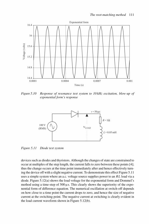
The root-matching method 111
Vol
tage
(vo
lts)
0.0001 0.0004 0.0007 0.00114.4
14.8
15.2
15.6
16
16.4
Time (s)
Exponential form
Figure 5.10 Response of resonance test system to 10 kHz excitation, blow-up ofexponential form’s response
100 V (RMS) VLOAD
� = 50 μs
L = 0.05 mH
R = 1Ω
Figure 5.11 Diode test system
devices such as diodes and thyristors. Although the changes of state are constrained tooccur at multiples of the step length, the current falls to zero between these points [4];thus the change occurs at the time point immediately after and hence effectively turn-ing the device off with a slight negative current. To demonstrate this effect Figure 5.11uses a simple system where an a.c. voltage source supplies power to an RL load via adiode. Figure 5.12(a) shows the load voltage for the exponential form and Dommel’smethod using a time-step of 500 μs. This clearly shows the superiority of the expo-nential form of difference equation. The numerical oscillation at switch-off dependson how close to a time point the current drops to zero, and hence the size of negativecurrent at the switching point. The negative current at switching is clearly evident inthe load current waveform shown in Figure 5.12(b).
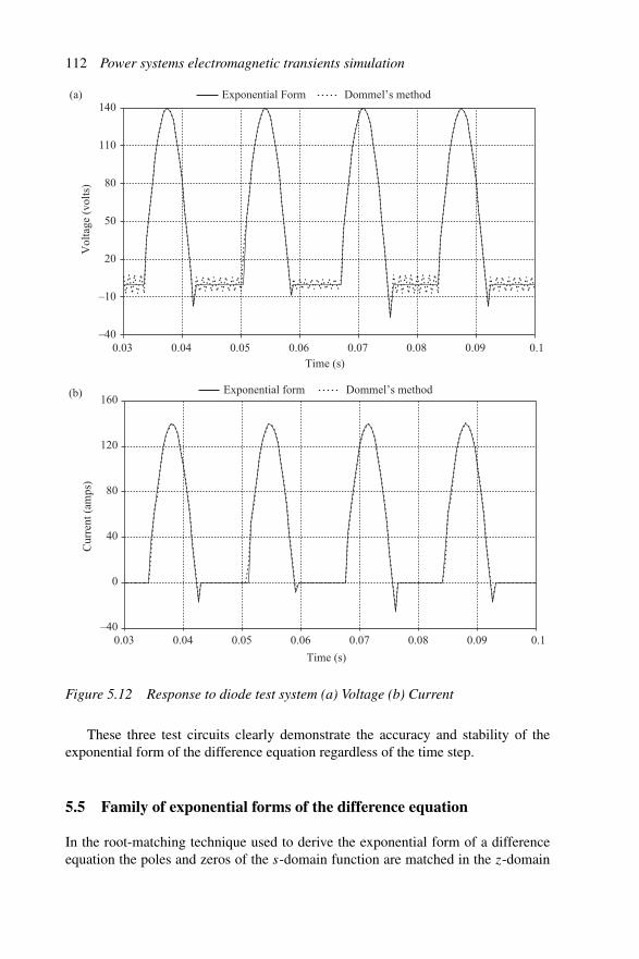
112 Power systems electromagnetic transients simulation
Vol
tage
(vo
lts)
Time (s)
Cur
rent
(am
ps)
Time (s)
–40
–10
20
50
80
110
140(a)
(b)
0.03 0.04 0.05 0.06 0.07 0.08 0.09 0.1
Exponential Form Dommel’s method
Exponential form Dommel’s method
–40
0
40
80
120
160
0.03 0.04 0.05 0.06 0.07 0.08 0.09 0.1
Figure 5.12 Response to diode test system (a) Voltage (b) Current
These three test circuits clearly demonstrate the accuracy and stability of theexponential form of the difference equation regardless of the time step.
5.5 Family of exponential forms of the difference equation
In the root-matching technique used to derive the exponential form of a differenceequation the poles and zeros of the s-domain function are matched in the z-domain

The root-matching method 113
u (t) u (t) u (t) u (t)
t t t t
(a) (b) (c) (d)
Figure 5.13 Input as function of time
u 1y
∑ R
L
G
R
R
1+ sL
1
Gs�
G1 + s�
1 + s�
H (s) =I (s)
V (s)H (s) =
==
Figure 5.14 Control or electrical system as first order lag
function. Extra zeros are added based on the assumed discretisation on the input,which is continuous [5]. Figure 5.13 shows some of the possible discretisationsand these result in a family of exponential forms of the difference equation. Theroot-matching technique is equally applicable to equations representing control orelectrical systems [6]. For each of the discretisation types, with reference to the firstorder lag function shown in Figure 5.14, the use of the root-matching techniqueexpressed as a rational function in z−1 produces the following exponential formdifference equations.
Input type (a):y(z)
u(z)= b/a(1 − e−a�t )
(1 − z−1e−a�t )
Input type (b):y(z)
u(z)= b/a(1 − e−a�t )z−1
(1 − z−1e−a�t )
Input type (c):y(z)
u(z)= b/(2a)(1 − e−a�t )(1 + z−1)
(1 − z−1e−a�t )

114 Power systems electromagnetic transients simulation
Input type (d):
y(z)
u(z)= b/a(−e−a�t + 1/(a�t)(1 − e−a�t ))z−1 + b/a(1 − 1/(a�t)(1 − e−a�t ))
(1 − z−1e−a�t )
Table E.3 (Appendix E) summarises the resulting difference equation for thefamily of exponential forms developed using root-matching techniques. The tablealso contains the difference equations derived from trapezoidal integrator substitution.The difference equations are then converted to the form:
(a0 + a1 z−1)/(b0 + b1 z−1) or (a′0 + a′
1z−1)/(1 + b1z
−1) if b0 is non-zero
Tables E.1 and E.2 give the coefficients of a rational function in z−1 that repre-sents each difference equation for the family of exponential forms, for admittanceand impedance respectively. It can be shown that the difference equation obtainedassuming type input (d) is identical to that obtained from the recursive convolutiontechnique developed by Semlyen and Dabuleanu [7].
5.5.1 Step response
A comparison of step responses is made here with reference to the simple switchingof a series RL branch, shown in Figure 5.2. Figure 5.15 shows the current magnitudeusing the difference equations generated by Dommel’s method, root-matching forinput types (a), (b), (c) and (d) and the theoretical result for �t = τ (τ = 50 μs).Figures 5.16 and 5.17 show the same comparison for �t = 5τ and �t = 10τ , respec-tively. Note that in the latter cases Dommel’s method exhibits numerical oscillation.Root-matching type (a) gives the exact answer at each time point as its discretisation ofthe input is exact. Root-matching type (b) gives the exact values but one time step lateas its discretisation of the input is a step occurring one time step later. Root-matchingtype (c) is an average between the previous two root-matching techniques.
Cur
rent
(am
ps)
Time (s)
Dommel Theoretical curve
0
20
40
60
80
100
0.00095 0.0012 0.00145
RM type A RM type B RM type C RM type D
Figure 5.15 Comparison of step response of switching test system for Δt = τ
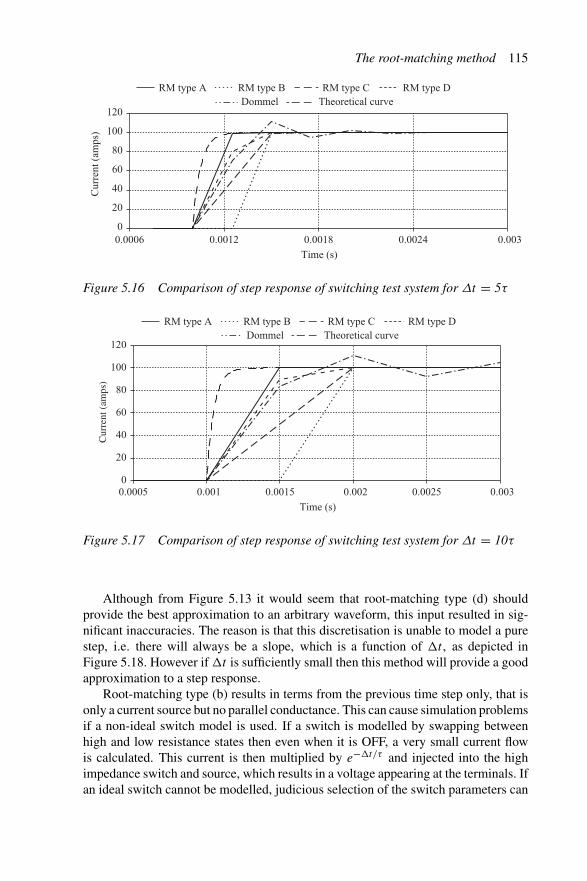
The root-matching method 115
Cur
rent
(am
ps)
Time (s)
0
20
40
60
80
100
120
0.0006 0.0012 0.0018 0.0024 0.003
Dommel Theoretical curveRM type A RM type B RM type C RM type D
Figure 5.16 Comparison of step response of switching test system for Δt = 5τ
Cur
rent
(am
ps)
Time (s)
0
20
40
60
80
100
120
0.0005 0.001 0.0015 0.002 0.0025 0.003
Dommel Theoretical curveRM type A RM type B RM type C RM type D
Figure 5.17 Comparison of step response of switching test system for Δt = 10τ
Although from Figure 5.13 it would seem that root-matching type (d) shouldprovide the best approximation to an arbitrary waveform, this input resulted in sig-nificant inaccuracies. The reason is that this discretisation is unable to model a purestep, i.e. there will always be a slope, which is a function of �t , as depicted inFigure 5.18. However if �t is sufficiently small then this method will provide a goodapproximation to a step response.
Root-matching type (b) results in terms from the previous time step only, that isonly a current source but no parallel conductance. This can cause simulation problemsif a non-ideal switch model is used. If a switch is modelled by swapping betweenhigh and low resistance states then even when it is OFF, a very small current flowis calculated. This current is then multiplied by e−�t/τ and injected into the highimpedance switch and source, which results in a voltage appearing at the terminals. Ifan ideal switch cannot be modelled, judicious selection of the switch parameters can
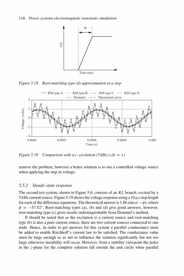
116 Power systems electromagnetic transients simulation
Δt
U(t
)
Time (ms)
Figure 5.18 Root-matching type (d) approximation to a step
Vol
tage
(vo
lts)
Time (s)
–4
–2
0
2
4
0.0046 0.0047 0.0048 0.0049 0.005
Dommel Theoretical curveRM type A RM type B RM type C RM type D
Figure 5.19 Comparison with a.c. excitation (5 kHz) (Δt = τ )
remove the problem, however a better solution is to use a controlled voltage sourcewhen applying the step in voltage.
5.5.2 Steady-state response
The second test system, shown in Figure 5.6, consists of an RL branch, excited by a5 kHz current source. Figure 5.19 shows the voltage response using a 10 μs step lengthfor each of the difference equations. The theoretical answer is 1.86 sin(ωt −φ), whereφ = −57.52◦. Root-matching types (a), (b) and (d) give good answers; however,root-matching type (c) gives results indistinguishable from Dommel’s method.
It should be noted that as the excitation is a current source and root-matchingtype (b) is also a pure current source, there are two current sources connected to onenode. Hence, in order to get answers for this system a parallel conductance mustbe added to enable Kirchhoff’s current law to be satisfied. The conductance valuemust be large enough so as not to influence the solution significantly but not toolarge otherwise instability will occur. However, from a stability viewpoint the polesin the z-plane for the complete solution fall outside the unit circle when parallel
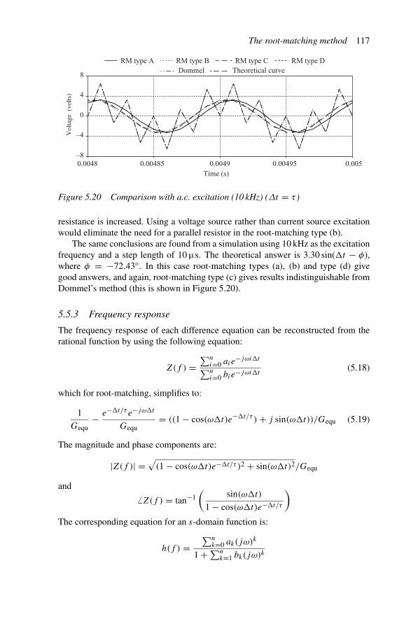
The root-matching method 117
Vol
tage
(vo
lts)
0.0048 0.00485 0.0049 0.00495 0.005Time (s)
–8
–4
0
4
8Dommel Theoretical curve
RM type A RM type B RM type C RM type D
Figure 5.20 Comparison with a.c. excitation (10 kHz) (Δt = τ )
resistance is increased. Using a voltage source rather than current source excitationwould eliminate the need for a parallel resistor in the root-matching type (b).
The same conclusions are found from a simulation using 10 kHz as the excitationfrequency and a step length of 10 μs. The theoretical answer is 3.30 sin(�t − φ),where φ = −72.43◦. In this case root-matching types (a), (b) and type (d) givegood answers, and again, root-matching type (c) gives results indistinguishable fromDommel’s method (this is shown in Figure 5.20).
5.5.3 Frequency response
The frequency response of each difference equation can be reconstructed from therational function by using the following equation:
Z(f ) =∑n
i=0 aie−jωi�t
∑ni=0 bie−jωi�t
(5.18)
which for root-matching, simplifies to:
1
Gequ− e−�t/τ e−jω�t
Gequ= ((1 − cos(ω�t)e−�t/τ ) + j sin(ω�t))/Gequ (5.19)
The magnitude and phase components are:
|Z(f )| =√
(1 − cos(ω�t)e−�t/τ )2 + sin(ω�t)2/Gequ
and� Z(f ) = tan−1
(sin(ω�t)
1 − cos(ω�t)e−�t/τ
)
The corresponding equation for an s-domain function is:
h(f ) =∑n
k=0 ak(jω)k
1 + ∑nk=1 bk(jω)k

118 Power systems electromagnetic transients simulation
RM type a RM type b RM type c RM type d DommelTheoretical
1
1.5
2
2.5
0 500 1000 1500 2000 2500 3000 3500 4000 4500 5000
0
20
40
60
80
100
120
0 500 1000 1500 2000 2500 3000 3500 4000 4500 5000Frequency (Hz)
Mag
nitu
deP
hase
(de
gs)
Figure 5.21 Frequency response for various simulation methods
The results of calculations performed using MATLAB (the code is given inAppendix F.4), are displayed in Figure 5.21. These results were verified by performinginjection tests into the appropriate difference equation using PSCAD/EMTDC sim-ulation software. As expected, the root-matching methods (a) and (b) provide theclosest match to the theoretical magnitude response, while root-matching methods(c) and (d) are similar to the trapezoidal rule. The phase response clearly shows thephase advance and phase lag inherent in the various discretisations used in the vari-ous root-matching methods. Root-matching method (a) shows the phase advance andmethod (b) the phase lag expected. Root-matching methods (c) and (d) and trapezoidalintegration show a considerably better phase response.
The trapezoidal rule assumes a linear variation between time points. An expo-nential form of the difference equation can also be derived assuming constant inputbetween solution points. Hence the exponential form of a circuit or transfer functionis not unique but depends on the assumed variation in input between time points.
5.6 Example
For the test system shown in Figure 5.2, if the switch is closed at t = 1.0 s the exactsolution is:
i(t) = VDC
R(1 − e−(t−1.0)/τ )
for t ≥ 1.0 where τ = L/R.
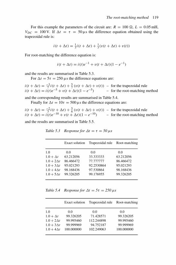
The root-matching method 119
For this example the parameters of the circuit are: R = 100 �, L = 0.05 mH,VDC = 100 V. If �t = τ = 50 μs the difference equation obtained using thetrapezoidal rule is:
i(t + �t) = 13 i(t + �t) + 1
3 (v(t + �t) + v(t))
For root-matching the difference equation is:
i(t + �t) = i(t)e−1 + v(t + �t)(1 − e−1)
and the results are summarised in Table 5.3.For �t = 5τ = 250 μs the difference equations are:
i(t + �t) = −37 i(t + �t) + 5
7 (v(t + �t) + v(t)) – for the trapezoidal rulei(t + �t) = i(t)e−5 + v(t + �t)(1 − e−5) – for the root-matching method
and the corresponding results are summarised in Table 5.4.Finally for �t = 10τ = 500 μs the difference equations are:
i(t + �t) = −23 i(t + �t) + 5
6 (v(t + �t) + v(t)) – for the trapezoidal rulei(t + �t) = i(t)e−10 + v(t + �t)(1 − e−10) – for the root-matching method
and the results are summarised in Table 5.5.
Table 5.3 Response for Δt = τ = 50 μs
Exact solution Trapezoidal rule Root-matching
1.0 0.0 0.0 0.01.0 + �t 63.212056 33.333333 63.2120561.0 + 2�t 86.466472 77.777777 86.4664721.0 + 3�t 95.021293 92.2530864 95.0212931.0 + 4�t 98.168436 97.530864 98.1684361.0 + 5�t 99.326205 99.176955 99.326205
Table 5.4 Response for Δt = 5τ = 250 μs
Exact solution Trapezoidal rule Root-matching
1.0 0.0 0.0 0.01.0 + �t 99.326205 71.428571 99.3262051.0 + 2�t 99.995460 112.244898 99.9954601.0 + 3�t 99.999969 94.752187 99.9999691.0 + 4�t 100.000000 102.249063 100.000000
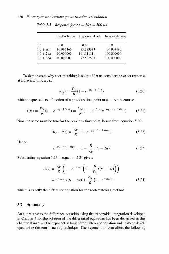
120 Power systems electromagnetic transients simulation
Table 5.5 Response for �t = 10τ = 500 μs
Exact solution Trapezoidal rule Root-matching
1.0 0.0 0.0 0.01.0 + �t 99.995460 83.333333 99.9954601.0 + 2�t 100.000000 111.111111 100.0000001.0 + 3�t 100.000000 92.592593 100.000000
To demonstrate why root-matching is so good let us consider the exact responseat a discrete time tk , i.e.
i(tk) = Vdc
R(1 − e−(tk−1.0)/τ ) (5.20)
which, expressed as a function of a previous time point at tk − �t , becomes:
i(tk) = Vdc
R(1 − e−(tk−1.0)/τ ) = Vdc
R(1 − e−�t/τ e−(tk−�t−1.0)/τ ) (5.21)
Now the same must be true for the previous time point, hence from equation 5.20:
i(tk − �t) = Vdc
R(1 − e−(tk−�t−1.0)/τ ) (5.22)
Hence
e−(tk−�t−1.0)/τ = 1 − R
Vdci(tk − �t) (5.23)
Substituting equation 5.23 in equation 5.21 gives:
i(tk) = Vdc
R
(1 − e−�t/τ
(1 − R
Vdci(tk − �t)
))
= e−�t/τ i(tk − �t) + Vdc
R
(1 − e−�t/τ
)(5.24)
which is exactly the difference equation for the root-matching method.
5.7 Summary
An alternative to the difference equation using the trapezoidal integration developedin Chapter 4 for the solution of the differential equations has been described in thischapter. It involves the exponential form of the difference equation and has been devel-oped using the root-matching technique. The exponential form offers the following
The root-matching method 121
advantages:
• Eliminates truncation errors, and hence numerical oscillations, regardless of thestep length used.
• Can be applied to both electrical networks and control blocks.• Can be viewed as a Norton equivalent in exactly the same way as the difference
equation developed by the numerical integration substitution (NIS) method.• It is perfectly compatible with NIS and the matrix solution technique remains
unchanged.• Provides highly efficient and accurate time domain simulation.
The exponential form can be implemented for all series and parallel RL, RC, LC
and RLC combinations, but not arbitrary components and hence is not a replacementfor NIS but a supplement.
5.8 References
1 WATSON, N. R. and IRWIN, G. D.: ‘Electromagnetic transient simulation of powersystems using root-matching techniques’, Proceedings IEE, Part C, 1998, 145 (5),pp. 481–6
2 ANGELIDIS, G. and SEMLYEN, A.: ‘Direct phase-domain calculation of trans-mission line transients using two-sided recursions’, IEEE Transactions on PowerDelivery, 1995, 10 (2), pp. 941–7
3 WATSON, N. R. and IRWIN, G. D.: ‘Accurate and stable electromagnetic transientsimulation using root-matching techniques’, International Journal of ElectricalPower & Energy Systems, Elsevier Science Ltd, 1999, 21 (3), pp. 225–34
4 CAMPOS-BARROS, J. G. and RANGEL, R. D.: ‘Computer simulation of modernpower systems: the elimination of numerical oscillation caused by valve action’,Proceedings of 4th International Conference on AC and DC Power Transmission,London, 1985, Vol. IEE Conf. Publ., 255, pp. 254–9
5 WATSON, N. R. and IRWIN, G. D.: ‘Comparison of root-matching techniquesfor electromagnetic transient simulation’, IEEE Transactions on Power Delivery,2000, 15 (2), pp. 629–34
6 WATSON, N. R., IRWIN, G. D. and NAYAK, O.: ‘Control modelling in electro-magnetic transient simulations’, Proceedings of International Conference on PowerSystem Transients (IPST’99), June 1999, pp. 544–8
7 SEMLYEN, A. and DABULEANU, A.: ‘Fast and accurate switching transientcalculations on transmission lines with ground return using recursive convolutions’,IEEE Transactions on Power Apparatus and Systems, 1975, 94 (2), pp. 561–71


Chapter 6
Transmission lines and cables
6.1 Introduction
Approximate nominal PI section models are often used for short transmission lines(of the order of 15 km), where the travel time is less than the solution time-step, butsuch models are unsuitable for transmission distances. Instead, travelling wave theoryis used in the development of more realistic models.
A simple and elegant travelling wave model of the lossless transmission line hasalready been described in Chapter 4 in the form of a dual Norton equivalent. Themodel is equally applicable to overhead lines and cables; the main differences arisefrom the procedures used in the calculation of the electrical parameters from theirrespective physical geometries. Carson’s solution [1] forms the basis of the overheadline parameter calculation, either as a numerical integration of Carson’s equation,the use of a series approximation or in the form of a complex depth of penetration.Underground cable parameters, on the other hand, are calculated using Pollack’sequations [2], [3].
Multiconductor lines have been traditionally accommodated in the EMTP by atransformation to natural modes to diagonalise the matrices involved. Original sta-bility problems were thought to be caused by inaccuracies in the modal domainrepresentation, and thus much of the effort went into the development of more accu-rate fitting techniques. More recently, Gustavsen and Semlyen [4] have shown that,although the phase domain is inherently stable, its associated modal domain may beinherently unstable regardless of the fitting. This revelation has encouraged a returnto the direct modelling of lines in the phase domain.
Figure 6.1 displays a decision tree for the selection of the appropriate transmissionline model. The minimum limit for travel time is Length/c where the c is the speedof light, and this can be compared to the time step to see if a PI section or travellingwave model is appropriate. Various PI section models exist, however the nominal(or coupled) PI, displayed in Figure 6.2, is the preferred option for transient solutions.The exact equivalent PI is only adequate for steady-state solution where only onefrequency is considered.
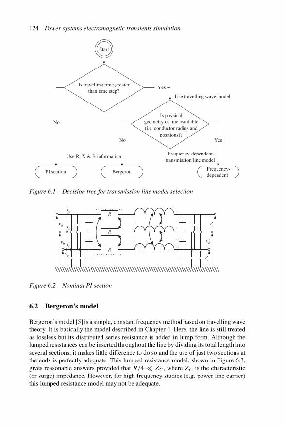
124 Power systems electromagnetic transients simulation
Is travelling time greater than time step?
Is physical geometry of line available (i.e. conductor radius and
positions)?
PI section BergeronFrequency-dependent
No
No Yes
Yes
Use travelling wave model
Use R, X & B informationFrequency-dependent
transmission line model
Start
Figure 6.1 Decision tree for transmission line model selection
Ria
ib
ic
va v�a
v�b
v�c
vb
vc
R
R
Figure 6.2 Nominal PI section
6.2 Bergeron’s model
Bergeron’s model [5] is a simple, constant frequency method based on travelling wavetheory. It is basically the model described in Chapter 4. Here, the line is still treatedas lossless but its distributed series resistance is added in lump form. Although thelumped resistances can be inserted throughout the line by dividing its total length intoseveral sections, it makes little difference to do so and the use of just two sections atthe ends is perfectly adequate. This lumped resistance model, shown in Figure 6.3,gives reasonable answers provided that R/4 � ZC , where ZC is the characteristic(or surge) impedance. However, for high frequency studies (e.g. power line carrier)this lumped resistance model may not be adequate.
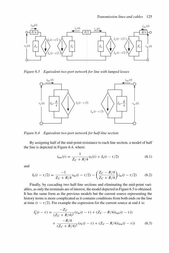
Transmission lines and cables 125
4R 4R2R
ZC CZ
ikm(t)
vk (t)
in (t)imk (t)
io (t)
vm (t)
Ik (t − �/2 ) Io (t − �/2 )
Im (t − �/2 )In (t − �/2 )
ZC ZC
Figure 6.3 Equivalent two-port network for line with lumped losses
ikm (t)
Ik (t – � /2)
Im (t – � /2)
vk (t) vm (t)
imk (t)
Z0 +R4
Z0 +R4
Figure 6.4 Equivalent two-port network for half-line section
By assigning half of the mid-point resistance to each line section, a model of halfthe line is depicted in Figure 6.4, where:
ikm(t) = 1
ZC + R/4vk(t) + Ik(t − τ/2) (6.1)
and
Ik(t − τ/2) = −1
ZC + R/4vm(t − τ/2) −
(ZC − R/4
ZC + R/4
)im(t − τ/2) (6.2)
Finally, by cascading two half-line sections and eliminating the mid-point vari-ables, as only the terminals are of interest, the model depicted in Figure 6.5 is obtained.It has the same form as the previous models but the current source representing thehistory terms is more complicated as it contains conditions from both ends on the lineat time (t − τ/2). For example the expression for the current source at end k is:
I ′k(t − τ) = −ZC
(ZC + R/4)2(vm(t − τ) + (ZC − R/4)imk(t − τ))
+ −R/4
(ZC + R/4)2(vk(t − τ) + (ZC − R/4)ikm(t − τ)) (6.3)

126 Power systems electromagnetic transients simulation
ikm (t)
Ik� (t – �)
Im� (t – �)
vk (t) vm (t)
imk (t)
Z0 +R4
Z0 +R4
Figure 6.5 Bergeron transmission line model
In the EMTDC program the line model separates the propagation into low and highfrequency paths, so that the line can have a higher attenuation to higher frequencies.This was an early attempt to provide frequency dependence, but newer models (in thephase domain) are now preferred.
6.2.1 Multiconductor transmission lines
Equations 4.22 and 4.23 are also applicable to multiconductor lines by replacing thescalar voltages and currents by vectors and using inductance and capacitance matrices.The wave propagation equations in the frequency domain are:
−[dVphase
dx
]=
[Z′
phase
][Iphase] (6.4)
−[dIphase
dx
]=
[Y ′
phase
][Vphase] (6.5)
By differentiating a second time, one vector, either the voltage or current, may beeliminated giving:
−[
d2Vphase
dx2
]
=[Z′
phase
] [dIphase
dx
]= −
[Z′
phase
][Y ′
phase][Vphase] (6.6)
−[
d2Iphase
dx2
]
=[Y ′
phase
] [dVphase
dx
]= −
[Y ′
phase
] [Z′
phase
][Iphase] (6.7)
Traditionally the complication of having off-diagonal elements in the matrices ofequations 6.6 and 6.7 is overcome by transforming into natural modes. Eigenvalueanalysis is applied to produce diagonal matrices, thereby transforming from coupledequations in the phase domain to decoupled equations in the modal domain. Eachequation in the modal domain is solved as for a single phase line by using modaltravelling time and modal surge impedance.

Transmission lines and cables 127
The transformation matrices between phase and modal quantities are different forvoltage and current, i.e.
[Vphase] = [Tv][Vmode] (6.8)
[Iphase] = [Ti][Imode] (6.9)
Substituting equation 6.8 in 6.6 gives:
[d2[Tv]Vmode
dx2
]=
[Z′
phase
] [Y ′
phase
][Tv][Vmode] (6.10)
Hence[d2Vmode
dx2
]= [Tv]−1
[Z′
phase
] [Y ′
phase
][Tv][Vmode] = [�][Vmode] (6.11)
To find the matrix [Tv] that diagonalises [Z′phase][Y ′
phase] its eigenvalues and eigen-vectors must be found. However the eigenvectors are not unique as when multipliedby a non-zero complex constant they are still valid eigenvectors, therefore somenormalisation is desirable to allow the output from different programs to be com-pared. PSCAD/EMTDC uses the root squaring technique developed by Wedepohl foreigenvalue analysis [6]. To enable us to generate frequency-dependent line modelsthe eigenvectors must be consistent from one frequency to the next, such that theeigenvectors form a continuous function of frequency so that curve fitting can beapplied. A Newton–Raphson algorithm has been developed for this purpose [6].
Once the eigenvalue analysis has been completed then:
[Zmode] = [Tv]−1[Zphase][Ti] (6.12)
[Ymode] = [Ti]−1[Yphase][Tv] (6.13)
[Zsurge i] =√
Zmode(i, i)
Ymode(i, i)(6.14)
where [Zmode] and [Ymode] are diagonal matrices.As the products [Z′
phase][Y ′phase] and [Y ′
phase][Z′phase] are different so are their
eigenvectors, even though their eigenvalues are identical. They are, however,related, such that [Ti] = ([Tv]T )−1 (assuming a normalised Euclidean norm, i.e.∑n
j=1 T 2ij = 1) and therefore only one of them needs to be calculated. Looking at
mode i, i.e. taking the ith equation from 6.11, gives:
[d2Vmode i
dx2
]= �iiVmode i (6.15)
and the general solution at point x in the line is:
Vmode i (x) = e−γ ixV Fmode i (k) + eγ ixV B
mode i (m) (6.16)
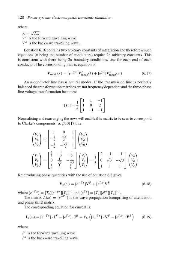
128 Power systems electromagnetic transients simulation
where
γi = √�ii
V F is the forward travelling waveV B is the backward travelling wave.
Equation 6.16 contains two arbitrary constants of integration and therefore n suchequations (n being the number of conductors) require 2n arbitrary constants. Thisis consistent with there being 2n boundary conditions, one for each end of eachconductor. The corresponding matrix equation is:
Vmode(x) = [e−γ x]VFmode(k) + [eγ x]VB
mode(m) (6.17)
An n-conductor line has n natural modes. If the transmission line is perfectlybalanced the transformation matrices are not frequency dependent and the three-phaseline voltage transformation becomes:
[Tv] = 1
k
⎡
⎣1 1 −11 0 21 −1 −1
⎤
⎦
Normalising and rearranging the rows will enable this matrix to be seen to correspondto Clarke’s components (α, β, 0) [7], i.e.
⎛
⎝Va
Vb
Vc
⎞
⎠ =
⎡
⎢⎢⎣
1 0 1
− 12
√3
2 1
− 12 −
√3
2 1
⎤
⎥⎥⎦
⎛
⎝Vα
Vβ
V0
⎞
⎠
⎛
⎝Vα
Vβ
V0
⎞
⎠ =⎡
⎢⎣
23 − 1
3 − 13
0 1√3
− 1√3
13
13
13
⎤
⎥⎦
⎛
⎝Va
Vb
Vc
⎞
⎠ = 1
3
⎡
⎢⎣
2 −1 −1
0√
3 −√3
1 1 1
⎤
⎥⎦
⎛
⎝Va
Vb
Vc
⎞
⎠
Reintroducing phase quantities with the use of equation 6.8 gives:
Vx(ω) = [e−�x]VF + [e�x]VB (6.18)
where [e−�x] = [Tv][e−γ x][Tv]−1 and [e�x] = [Tv][eγ x][Tv]−1.The matrix A(ω) = [e−�x] is the wave propagation (comprising of attenuation
and phase shift) matrix.The corresponding equation for current is:
Ix(ω) = [e−�x] · IF − [e�x] · IB = YC
([e−�x] · VF − [e�x] · VB
)(6.19)
where
IF is the forward travelling waveIB is the backward travelling wave.
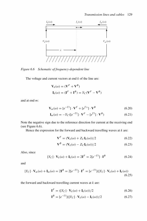
Transmission lines and cables 129
x
Ik (�) Ix (�)
Vk (�) Vm (�)
Im (�)
Figure 6.6 Schematic of frequency-dependent line
The voltage and current vectors at end k of the line are:
Vk(ω) = (VF + VB)
Ik(ω) = (IF + IB) = YC(VF − VB)
and at end m:
Vm(ω) = [e−�l] · VF + [e�x] · VB (6.20)
Im(ω) = −YC([e−�l] · VF − [e�l] · VB) (6.21)
Note the negative sign due to the reference direction for current at the receiving end(see Figure 6.6).
Hence the expression for the forward and backward travelling waves at k are:
VF = (Vk(ω) + ZCIk(ω))/2 (6.22)
VB = (Vk(ω) − ZCIk(ω))/2 (6.23)
Also, since[YC] · Vk(ω) + Ik(ω) = 2IF = 2[e−�l] · IB (6.24)
and
[YC] · Vm(ω) + Im(ω) = 2IB = 2[e−�l] · IF = [e−�l]([YC] · Vk(ω) + Ik(ω))
(6.25)
the forward and backward travelling current waves at k are:
IF = ([YC] · Vk(ω) + Ik(ω))/2 (6.26)
IB = [e−�l]([YC] · Vk(ω) − Ik(ω))/2 (6.27)
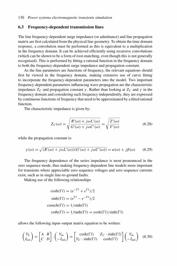
130 Power systems electromagnetic transients simulation
6.3 Frequency-dependent transmission lines
The line frequency-dependent surge impedance (or admittance) and line propagationmatrix are first calculated from the physical line geometry. To obtain the time domainresponse, a convolution must be performed as this is equivalent to a multiplicationin the frequency domain. It can be achieved efficiently using recursive convolutions(which can be shown to be a form of root-matching, even though this is not generallyrecognised). This is performed by fitting a rational function in the frequency domainto both the frequency-dependent surge impedance and propagation constant.
As the line parameters are functions of frequency, the relevant equations shouldfirst be viewed in the frequency domain, making extensive use of curve fittingto incorporate the frequency-dependent parameters into the model. Two importantfrequency-dependent parameters influencing wave propagation are the characteristicimpedance ZC and propagation constant γ . Rather than looking at ZC and γ in thefrequency domain and considering each frequency independently, they are expressedby continuous functions of frequency that need to be approximated by a fitted rationalfunction.
The characteristic impedance is given by:
ZC(ω) =√
R′(ω) + jωL′(ω)
G′(ω) + jωC′(ω)=
√Z′(ω)
Y ′(ω)(6.28)
while the propagation constant is:
γ (ω) = √(R′(ω) + jωL′(ω))(G′(ω) + jωC′(ω)) = α(ω) + jβ(ω) (6.29)
The frequency dependence of the series impedance is most pronounced in thezero sequence mode, thus making frequency-dependent line models more importantfor transients where appreciable zero sequence voltages and zero sequence currentsexist, such as in single line-to-ground faults.
Making use of the following relationships
cosh(�l) = (e−�l + e�l)/2
sinh(�l) = (e�l − e−�l)/2
cosech(�l) = 1/sinh(�l)
coth(�l) = 1/tanh(�l) = cosh(�l)/sinh(�l)
allows the following input–output matrix equation to be written:
(Vk
Ikm
)=
[A B
C D
].
(Vm
−Imk
)=
[cosh(�l) ZC · sinh(�l)
YC · sinh(�l) cosh(�l)
](Vm
−Imk
)(6.30)

Transmission lines and cables 131
Rearranging equation 6.30 leads to the following two-port representation:
(Ikm
Imk
)=
[D · B−1 C − D · B−1A
−B B−1A
](Vk
Vm
)
=[
YC · coth(�l) −YC · cosech(�l)
−YC · cosech(�l) YC · coth(�l)
](Vk
Vm
)(6.31)
and using the conversion between the modal and phase domains, i.e.
[coth(�l)] = [Tv] · [coth(γ (ω)l)] · [Tv]−1 (6.32)
[cosech(�l)] = [Tv] · [cosech(γ (ω)l)] · [Tv]−1 (6.33)
the exact a.c. steady-state input–output relationship of the line at any frequency is:
(Vk(ω)
Ikm(ω)
)=
⎡
⎣cosh(γ (ω)l) ZC sinh(γ (ω)l)
1
ZC
sinh(γ (ω)l) cosh(γ (ω)l)
⎤
⎦(
Vm(ω)
−Imk(ω)
)(6.34)
This clearly shows the Ferranti effect in an open circuit line, because the ratio
Vm(ω)/Vk(ω) = 1/cosh(γ (ω)l)
increases with line length and frequency.The forward and backward travelling waves at end k are:
Fk(ω) = Vk(ω) + ZC(ω)Ik(ω) (6.35)
Bk(ω) = Vk(ω) − ZC(ω)Ik(ω) (6.36)
and similarly for end m:
Fm(ω) = Vm(ω) + ZC(ω)Im(ω) (6.37)
Bm(ω) = Vm(ω) − ZC(ω)Im(ω) (6.38)
Equation 6.36 can be viewed as a Thevenin circuit (shown in Figure 6.7) whereVk(ω) is the terminal voltage, Bk(ω) the voltage source and characteristic or surgeimpedance, ZC(ω), the series impedance.
The backward travelling wave at k is the forward travelling wave at m multipliedby the wave propagation matrix, i.e.
Bk(ω) = A(ω)Fm(ω) (6.39)
Rearranging equation 6.35 to give Vk(ω), and substituting in equation 6.39, then usingequation 6.37 to eliminate Fm(ω) gives:
Vk(ω) = ZC(ω)Ik(ω) + A(ω)(Vm(ω) + Zm(ω)Im(ω)) (6.40)
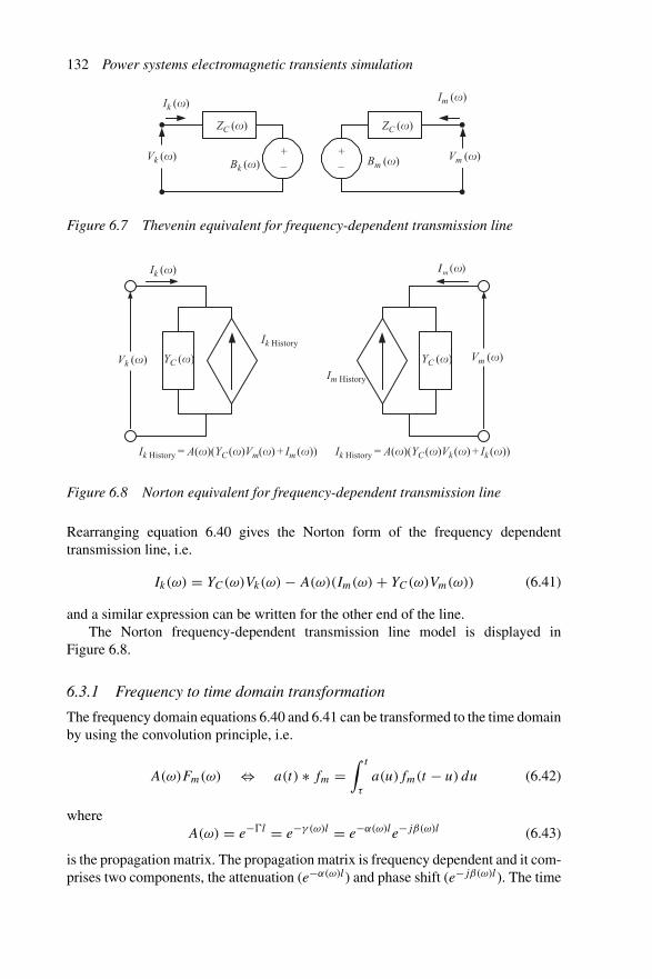
132 Power systems electromagnetic transients simulation
+–
+–
Vk (�) Vm (�)
Im (�)
Bk (�) Bm (�)
ZC (�)
Ik (�)
ZC (�)
Figure 6.7 Thevenin equivalent for frequency-dependent transmission line
Ik (�) )(�mI
YC (�) YC (�)Vk (�) Vm (�)
Ik History
Im History
Ik History = A(�)(YC (�)Vm(�) + Im (�)) Ik History = A(�)(YC (�)Vk (�) + Ik (�))
Figure 6.8 Norton equivalent for frequency-dependent transmission line
Rearranging equation 6.40 gives the Norton form of the frequency dependenttransmission line, i.e.
Ik(ω) = YC(ω)Vk(ω) − A(ω)(Im(ω) + YC(ω)Vm(ω)) (6.41)
and a similar expression can be written for the other end of the line.The Norton frequency-dependent transmission line model is displayed in
Figure 6.8.
6.3.1 Frequency to time domain transformation
The frequency domain equations 6.40 and 6.41 can be transformed to the time domainby using the convolution principle, i.e.
A(ω)Fm(ω) ⇔ a(t) ∗ fm =∫ t
τ
a(u)fm(t − u) du (6.42)
whereA(ω) = e−�l = e−γ (ω)l = e−α(ω)le−jβ(ω)l (6.43)
is the propagation matrix. The propagation matrix is frequency dependent and it com-prises two components, the attenuation (e−α(ω)l) and phase shift (e−jβ(ω)l). The time

Transmission lines and cables 133
domain equivalent of these are a(t) and β, where a(t) is the time domain transform(impulse response) of e−α(ω)l and β is a pure time delay (travelling time). The lowerlimit of the integral in equation 6.42, τ , is the time (in seconds) for an impulse totravel from one end of the line to the other.
Thus converting equations 6.40 and 6.41 to the time domain yields:
vk(t) = ZC(t) ∗ ikm(t) + a(t) ∗ (vm(t) + ZC(t) ∗ imk(t)) (6.44)
ik(t) = YC(t) ∗ vk(t) − a(t) ∗ (YC(t) ∗ vm(t − τ) − im(t − τ)) (6.45)
This process can be evaluated efficiently using recursive convolution if a(u) is anexponential. This is achieved using the partial fraction expansion of a rational func-tion to represent A(ω) in the frequency domain as the inverse Laplace transform ofkm/(s + pm) which is km · e−pmt . Hence the convolution of equation 6.42 becomes:
y(t) = km
∫ t
τ
e−pm(T )fm(t − T ) dT (6.46)
Semlyen and Dabuleanu [8] showed that for a single time step the above equationyields:
y(t) = e−pm�t · y(t − �t) +∫ �t
0kme−pmT u (t − T ) dT (6.47)
It is a recursive process because y(t) is found from y(t − �t) with a simpleintegration over one single time step. If the input is assumed constant during the timestep, it can be taken outside the integral, which can then be determined analytically, i.e.
y(t) = e−pm�ty(t − �t) + u(t − �t)
∫ �t
0kme−pmT dT (6.48)
= e−pm�ty(t − �t) + km
pm
(1 − e−pm�t )u(t − �t) (6.49)
If the input is assumed to vary linearly, i.e.
u(t − T ) = (u(t − �t) − u(t))
�tT + u(t) (6.50)
the resulting recursive equation becomes:
y(t) = e−pm�txn−1 + km
pm
(1 − 1
pm�t(1 − e−a�t )
)u(t)
+ km
pm
(−e−a�t + 1
pm�t(1 − e−a�t )
)u(t − �t) (6.51)
The propagation constant can be approximated by the following rational function
Aapprox(s) = e−sτ (s + z1)(s + z2) · · · (s + zn)
(s + p1)(s + p2) · · · (s + pm)(6.52)
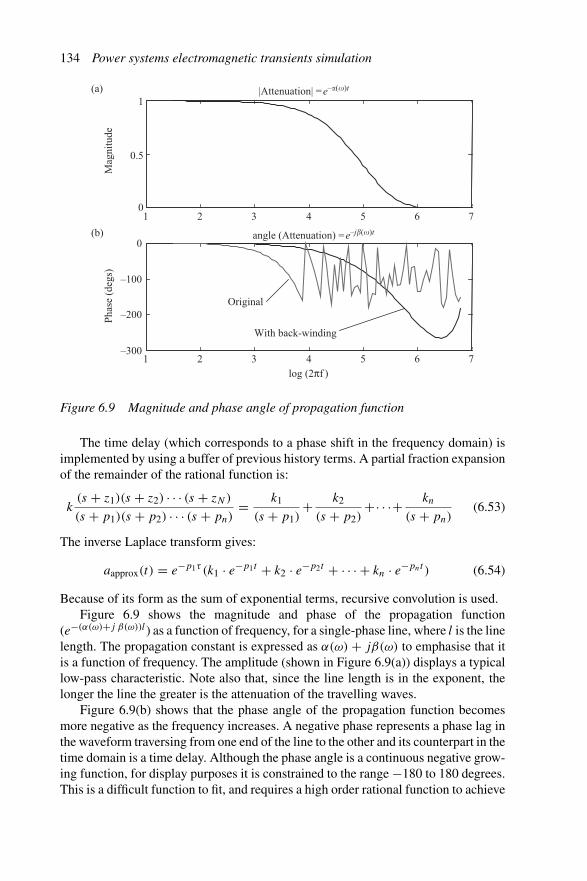
134 Power systems electromagnetic transients simulation
1 2 3 4 5 6 7
1 2 3 4 5 6 7log (2πf )
angle (Attenuation) =e–j�(�)t
|Attenuation| =e–�(�)t
Original
With back-winding
–300
–200
–100
0
0
0.5
1M
agni
tude
Pha
se (
degs
)
(a)
(b)
Figure 6.9 Magnitude and phase angle of propagation function
The time delay (which corresponds to a phase shift in the frequency domain) isimplemented by using a buffer of previous history terms. A partial fraction expansionof the remainder of the rational function is:
k(s + z1)(s + z2) · · · (s + zN)
(s + p1)(s + p2) · · · (s + pn)= k1
(s + p1)+ k2
(s + p2)+· · ·+ kn
(s + pn)(6.53)
The inverse Laplace transform gives:
aapprox(t) = e−p1τ (k1 · e−p1t + k2 · e−p2t + · · · + kn · e−pnt ) (6.54)
Because of its form as the sum of exponential terms, recursive convolution is used.Figure 6.9 shows the magnitude and phase of the propagation function
(e−(α(ω)+j β(ω))l) as a function of frequency, for a single-phase line, where l is the linelength. The propagation constant is expressed as α(ω) + jβ(ω) to emphasise that itis a function of frequency. The amplitude (shown in Figure 6.9(a)) displays a typicallow-pass characteristic. Note also that, since the line length is in the exponent, thelonger the line the greater is the attenuation of the travelling waves.
Figure 6.9(b) shows that the phase angle of the propagation function becomesmore negative as the frequency increases. A negative phase represents a phase lag inthe waveform traversing from one end of the line to the other and its counterpart in thetime domain is a time delay. Although the phase angle is a continuous negative grow-ing function, for display purposes it is constrained to the range −180 to 180 degrees.This is a difficult function to fit, and requires a high order rational function to achieve
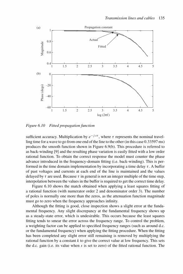
Transmission lines and cables 135
Propagation constant
Actual
Fitted
log (2πf )
0.4
0.6
0.8
1
–60
–40
–20
0
1 1.5 2 2.5 3 3.5 4 4.5 5
1 1.5 2 2.5 3 3.5 4 4.5 5
Mag
nitu
deP
hase
(de
gs)
(a)
(b)
Figure 6.10 Fitted propagation function
sufficient accuracy. Multiplication by e−j sτ , where τ represents the nominal travel-ling time for a wave to go from one end of the line to the other (in this case 0.33597 ms)produces the smooth function shown in Figure 6.9(b). This procedure is referred toas back-winding [9] and the resulting phase variation is easily fitted with a low orderrational function. To obtain the correct response the model must counter the phaseadvance introduced in the frequency-domain fitting (i.e. back-winding). This is per-formed in the time domain implementation by incorporating a time delay τ . A bufferof past voltages and currents at each end of the line is maintained and the valuesdelayed by τ are used. Because τ in general is not an integer multiple of the time step,interpolation between the values in the buffer is required to get the correct time delay.
Figure 6.10 shows the match obtained when applying a least squares fitting ofa rational function (with numerator order 2 and denominator order 3). The numberof poles is normally one more than the zeros, as the attenuation function magnitudemust go to zero when the frequency approaches infinity.
Although the fitting is good, close inspection shows a slight error at the funda-mental frequency. Any slight discrepancy at the fundamental frequency shows upas a steady-state error, which is undesirable. This occurs because the least squaresfitting tends to smear the error across the frequency range. To control the problem,a weighting factor can be applied to specified frequency ranges (such as around d.c.or the fundamental frequency) when applying the fitting procedure. When the fittinghas been completed any slight error still remaining is removed by multiplying therational function by a constant k to give the correct value at low frequency. This setsthe d.c. gain (i.e. its value when s is set to zero) of the fitted rational function. The
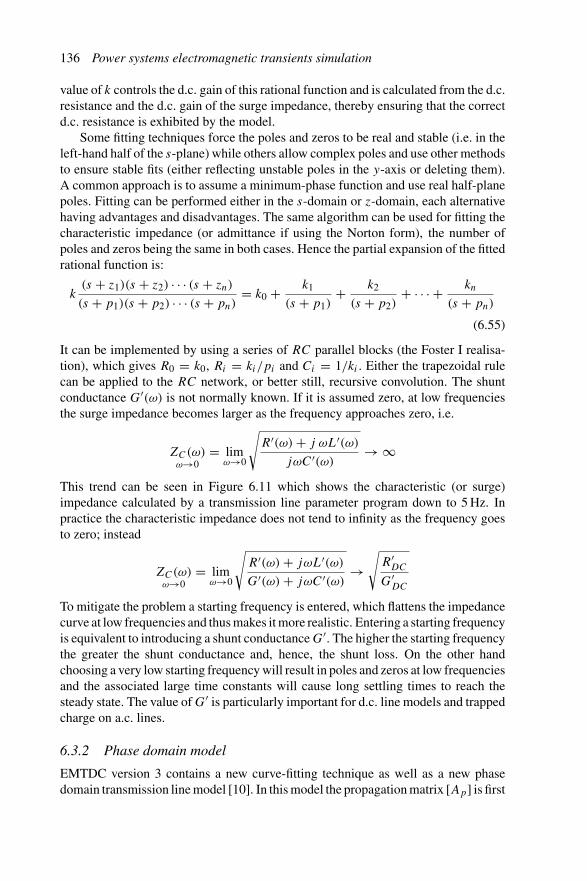
136 Power systems electromagnetic transients simulation
value of k controls the d.c. gain of this rational function and is calculated from the d.c.resistance and the d.c. gain of the surge impedance, thereby ensuring that the correctd.c. resistance is exhibited by the model.
Some fitting techniques force the poles and zeros to be real and stable (i.e. in theleft-hand half of the s-plane) while others allow complex poles and use other methodsto ensure stable fits (either reflecting unstable poles in the y-axis or deleting them).A common approach is to assume a minimum-phase function and use real half-planepoles. Fitting can be performed either in the s-domain or z-domain, each alternativehaving advantages and disadvantages. The same algorithm can be used for fitting thecharacteristic impedance (or admittance if using the Norton form), the number ofpoles and zeros being the same in both cases. Hence the partial expansion of the fittedrational function is:
k(s + z1)(s + z2) · · · (s + zn)
(s + p1)(s + p2) · · · (s + pn)= k0 + k1
(s + p1)+ k2
(s + p2)+ · · · + kn
(s + pn)
(6.55)
It can be implemented by using a series of RC parallel blocks (the Foster I realisa-tion), which gives R0 = k0, Ri = ki/pi and Ci = 1/ki . Either the trapezoidal rulecan be applied to the RC network, or better still, recursive convolution. The shuntconductance G′(ω) is not normally known. If it is assumed zero, at low frequenciesthe surge impedance becomes larger as the frequency approaches zero, i.e.
ZC(ω)ω→0
= limω→0
√R′(ω) + j ωL′(ω)
jωC′(ω)→ ∞
This trend can be seen in Figure 6.11 which shows the characteristic (or surge)impedance calculated by a transmission line parameter program down to 5 Hz. Inpractice the characteristic impedance does not tend to infinity as the frequency goesto zero; instead
ZC(ω)ω→0
= limω→0
√R′(ω) + jωL′(ω)
G′(ω) + jωC′(ω)→
√R′
DC
G′DC
To mitigate the problem a starting frequency is entered, which flattens the impedancecurve at low frequencies and thus makes it more realistic. Entering a starting frequencyis equivalent to introducing a shunt conductance G′. The higher the starting frequencythe greater the shunt conductance and, hence, the shunt loss. On the other handchoosing a very low starting frequency will result in poles and zeros at low frequenciesand the associated large time constants will cause long settling times to reach thesteady state. The value of G′ is particularly important for d.c. line models and trappedcharge on a.c. lines.
6.3.2 Phase domain model
EMTDC version 3 contains a new curve-fitting technique as well as a new phasedomain transmission line model [10]. In this model the propagation matrix [Ap] is first
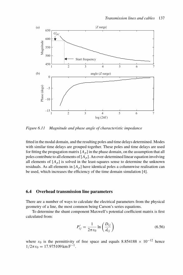
Transmission lines and cables 137
Mag
nitu
de
|Z surge|
1 2 3 4 5 6 7log (2πf )
Pha
se (
degs
)
angle (Z surge)
G�DC
Start frequency
450
500
550
600
650
1 2 3 4 5 6 7
–15
–10
–5
0
(a)
(b)
Figure 6.11 Magnitude and phase angle of characteristic impedance
fitted in the modal domain, and the resulting poles and time delays determined. Modeswith similar time delays are grouped together. These poles and time delays are usedfor fitting the propagation matrix [Ap] in the phase domain, on the assumption that allpoles contribute to all elements of [Ap]. An over-determined linear equation involvingall elements of [Ap] is solved in the least-squares sense to determine the unknownresiduals. As all elements in [Ap] have identical poles a columnwise realisation canbe used, which increases the efficiency of the time domain simulation [4].
6.4 Overhead transmission line parameters
There are a number of ways to calculate the electrical parameters from the physicalgeometry of a line, the most common being Carson’s series equations.
To determine the shunt component Maxwell’s potential coefficient matrix is firstcalculated from:
P ′ij = 1
2πε0ln
(Dij
dij
)(6.56)
where ε0 is the permittivity of free space and equals 8.854188 × 10⁻¹² hence1/2πε0 = 17.975109 km F−1.

138 Power systems electromagnetic transients simulation
dij
i
Image of conductors
Ground
i�
j�
j
Yi – Yj
Yi + Yj
Yj
Yi
2Yi
Xi – Xj
ij
Dij
Figure 6.12 Transmission line geometry
if i �= j
Dij =√
(Xi − Xj)2 − (Yi + Yj )2
dij =√
(Xi − Xj)2 − (Yi − Yj )2
if i = j
Dij = 2Yi
dij = GMRi (bundled conductor) or Ri (radius for single conductor)
In Figure 6.12 the conductor heights Yi and Yj are the average heights aboveground which are Ytower − 2/3Ysag.
Maxwell’s potential coefficient matrix relates the voltages to the charge per unitlength, i.e.
V = [P ′]qHence the capacitance matrix is given by
[C] = [P ′]−1 (6.57)
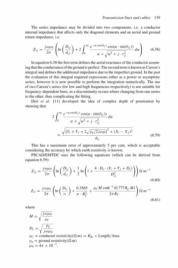
Transmission lines and cables 139
The series impedance may be divided into two components, i.e. a conductorinternal impedance that affects only the diagonal elements and an aerial and groundreturn impedance, i.e.
Zij = jωμ0
2π
⎛
⎝ln
(Dij
dij
)+ 2
∫ ∞
0
e−α·cos(θij ) cos(α · sin(θij ))
α +√
α2 + j · r2ij
dα
⎞
⎠ (6.58)
In equation 6.58 the first term defines the aerial reactance of the conductor assum-ing that the conductance of the ground is perfect. The second term is known as Carson’sintegral and defines the additional impedance due to the imperfect ground. In the pastthe evaluation of this integral required expressions either as a power or asymptoticseries; however it is now possible to perform the integration numerically. The useof two Carson’s series (for low and high frequencies respectively) is not suitable forfrequency-dependent lines, as a discontinuity occurs where changing from one seriesto the other, thus complicating the fitting.
Deri et al. [11] developed the idea of complex depth of penetration byshowing that:
2∫ ∞
0
e−α·cos(θij ) cos(α · sin(θij ))
α +√
α2 + j · r2ij
dα
≈√(
Yi + Yj + 2√
ρg/2jωμ)2 + (Xi − Xj)2
dij
(6.59)
This has a maximum error of approximately 5 per cent, which is acceptableconsidering the accuracy by which earth resistivity is known.
PSCAD/EMTDC uses the following equations (which can be derived fromequation 6.59):
Zij = jωμ0
2π
(
ln
(Dij
dij
)+ 1
2ln
(
1 + 4 · De · (Yi + Yj + De)
D2ij
))
� m−1
(6.60)
Zii = jωμ0
2π
(
ln
(Dii
ri
)+ 0.3565
π · R2C
+ ρCM coth−1(0.777RCM)
2πRC
)
� m−1
(6.61)
where
M =√
jωμ0
ρC
De =√
ρg
jωμ0ρC = conductor resistivity(� m) = Rdc × Length/Areaρg = ground resistivity(� m)
μ0 = 4π × 10−7.
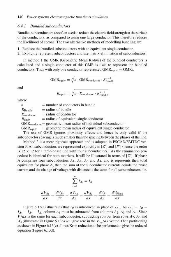
140 Power systems electromagnetic transients simulation
6.4.1 Bundled subconductors
Bundled subconductors are often used to reduce the electric field strength at the surfaceof the conductors, as compared to using one large conductor. This therefore reducesthe likelihood of corona. The two alternative methods of modelling bundling are:
1. Replace the bundled subconductors with an equivalent single conductor.2. Explicitly represent subconductors and use matrix elimination of subconductors.
In method 1 the GMR (Geometric Mean Radius) of the bundled conductors iscalculated and a single conductor of this GMR is used to represent the bundledconductors. Thus with only one conductor represented GMRequiv = GMRi .
GMRequiv = n
√n · GMRconductor · Rn−1
Bundle
and
Requiv = n
√n · Rconductor · Rn−1
Bundle
wheren = number of conductors in bundleRBundle = radius of bundleRconductor = radius of conductorRequiv = radius of equivalent single conductorGMRconductor= geometric mean radius of individual subconductorGMRequiv = geometric mean radius of equivalent single conductor.
The use of GMR ignores proximity effects and hence is only valid if thesubconductor spacing is much smaller than the spacing between the phases of the line.
Method 2 is a more rigorous approach and is adopted in PSCAD/EMTDC ver-sion 3. All subconductors are represented explicitly in [Z′] and [P ′] (hence the orderis 12 × 12 for a three-phase line with four subconductors). As the elimination pro-cedure is identical for both matrices, it will be illustrated in terms of [Z′]. If phaseA comprises four subconductors A1, A2, A3 and A4, and R represents their totalequivalent for phase A, then the sum of the subconductor currents equals the phasecurrent and the change of voltage with distance is the same for all subconductors, i.e.
n∑
i=1
IAi= IR
dVA1
dx= dVA2
dx= dVA3
dx= dVA4
dx= dVR
dx= dVPhase
dx
Figure 6.13(a) illustrates that IR is introduced in place of IA1 . As IA1 = IR −IA2 − IA3 − IA4 column A1 must be subtracted from columns A2, A3 and A4. SinceV/dx is the same for each subconductor, subtracting row A1 from rows A2, A3 andA4 (illustrated in Figure 6.13b) will give zero in the VA2/dx vector. Then partitioningas shown in Figure 6.13(c) allows Kron reduction to be performed to give the reducedequation (Figure 6.13d).
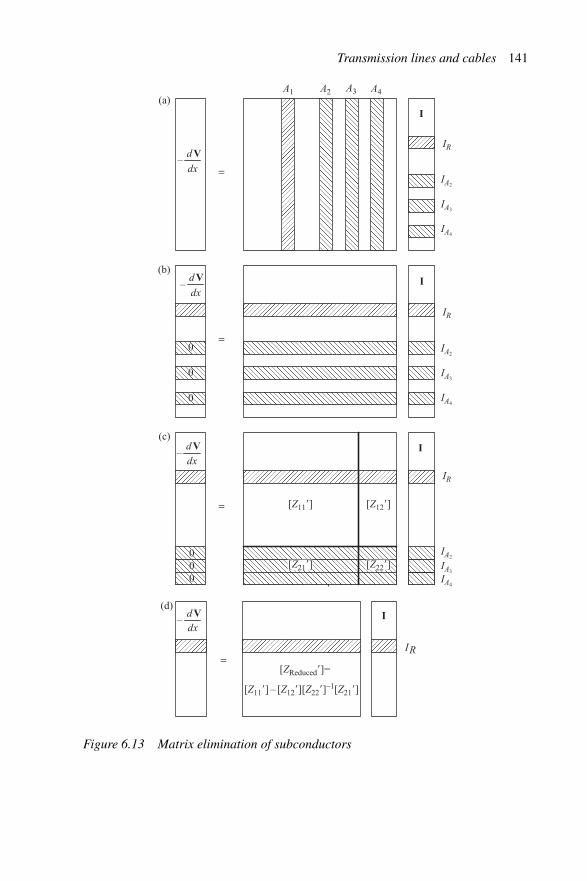
Transmission lines and cables 141
A2A1 A3 A4
d V
dx
IR
=IA2
IA3
IA4
IA2
IA3
IA4
IR
IR
IA2
IA3
IA4
=0
0
0
=
000
0
0
0
000
'
RI=
[ZReduced�]=
I
d V
dx–
d V
dx–
–d Vdx
I
I
I
(a)
(b)
(c)
(d)
[Z21�]
[Z11�] – [Z12�][Z22�]–1[Z21�]
[Z22�]
[Z11�] [Z12�]
–
Figure 6.13 Matrix elimination of subconductors

142 Power systems electromagnetic transients simulation
External
Loop 1
Loop 2
Loop 3C
S
A
X
Figure 6.14 Cable cross-section
This method does include proximity effects and hence is generally more accu-rate; however the difference with respect to using one equivalent single conductorof appropriate GMR is very small when the phase spacing is much greater than thebundle spacing.
6.4.2 Earth wires
When earth wires are continuous and grounded at each tower then for frequenciesbelow 250 kHz it is reasonable to assume that the earth wire potential is zero along itslength. The reduction procedure for [Z′] and [P ′] is the same. [P ′] is reduced priorto inverting to give the capacitance matrix. The matrix reduction is next illustratedfor the series impedance.
Assuming a continuous earth wire grounded at each tower then dVe/dx = 0 andVe = 0. Partitioning into conductors and earth wires gives:
−
⎛
⎜⎜⎝
(dVc
dx
)
(dVe
dx
)
⎞
⎟⎟⎠ = −
⎛
⎝
(dVc
dx
)
(0)
⎞
⎠ =[[
Z′cc
] [Z′
ce
]
[Z′
ec
] [Z′
ee
]
]((Ic)
(Ie)
)(6.62)
−(
dVc
dx
)= [ZReduced′ ](Ic)
where [ZReduced′ ] = [Z′
cc
] − [Z′
ce
] [Z′
ee
]−1 [Z′
ec
].
When the earth wires are bundled the same technique used for bundled phasesubconductors can be applied to them.
6.5 Underground cable parameters
A unified solution similar to that of overhead transmission is difficult for undergroundcables because of the great variety in their construction and layouts.
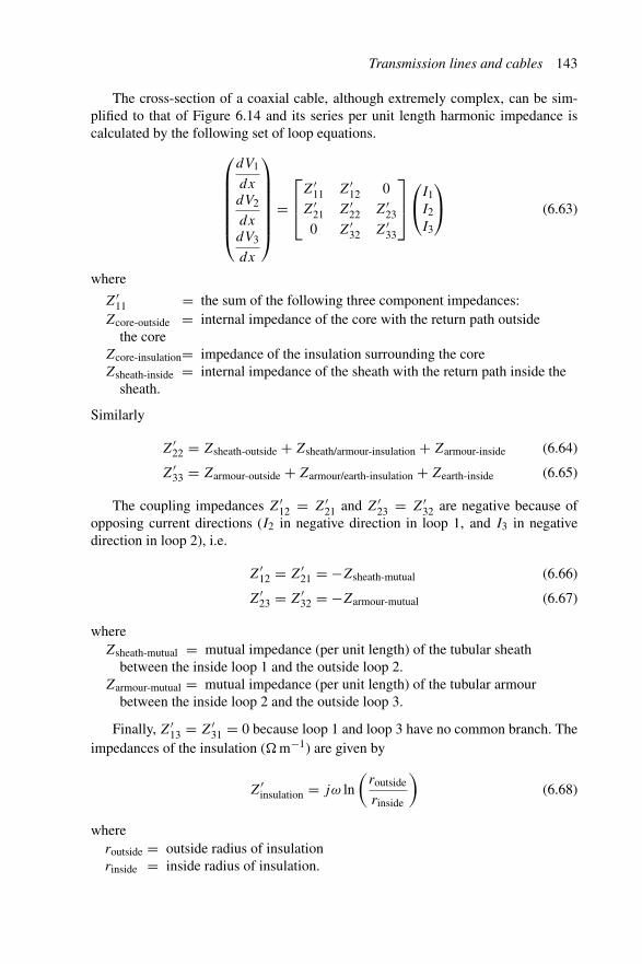
Transmission lines and cables 143
The cross-section of a coaxial cable, although extremely complex, can be sim-plified to that of Figure 6.14 and its series per unit length harmonic impedance iscalculated by the following set of loop equations.
⎛
⎜⎜⎜⎜⎜⎜⎝
dV1
dx
dV2
dx
dV3
dx
⎞
⎟⎟⎟⎟⎟⎟⎠
=⎡
⎢⎣
Z′11 Z′
12 0
Z′21 Z′
22 Z′23
0 Z′32 Z′
33
⎤
⎥⎦
⎛
⎝I1I2I3
⎞
⎠ (6.63)
where
Z′11 = the sum of the following three component impedances:
Zcore-outside = internal impedance of the core with the return path outsidethe core
Zcore-insulation= impedance of the insulation surrounding the coreZsheath-inside = internal impedance of the sheath with the return path inside the
sheath.
Similarly
Z′22 = Zsheath-outside + Zsheath/armour-insulation + Zarmour-inside (6.64)
Z′33 = Zarmour-outside + Zarmour/earth-insulation + Zearth-inside (6.65)
The coupling impedances Z′12 = Z′
21 and Z′23 = Z′
32 are negative because ofopposing current directions (I2 in negative direction in loop 1, and I3 in negativedirection in loop 2), i.e.
Z′12 = Z′
21 = −Zsheath-mutual (6.66)
Z′23 = Z′
32 = −Zarmour-mutual (6.67)
whereZsheath-mutual = mutual impedance (per unit length) of the tubular sheath
between the inside loop 1 and the outside loop 2.Zarmour-mutual = mutual impedance (per unit length) of the tubular armour
between the inside loop 2 and the outside loop 3.
Finally, Z′13 = Z′
31 = 0 because loop 1 and loop 3 have no common branch. Theimpedances of the insulation (� m−1) are given by
Z′insulation = jω ln
(routside
rinside
)(6.68)
whereroutside = outside radius of insulationrinside = inside radius of insulation.

144 Power systems electromagnetic transients simulation
If there is no insulation between the armour and earth, then Zinsulation = 0. Theinternal impedances and the mutual impedance of a tubular conductor are a functionof frequency, and can be derived from Bessel and Kelvin functions.
Z′tube-inside = jωμ
2πD · mq[I0(mq)K1(mr) + K0(mq)I1(mr)] (6.69)
Z′tube-outside = jωμ
2πD · mr[I0(mr)K1(mq) + K0(mr)I1(mq)] (6.70)
Z′tube-mutual = jωμ
2πD · mq · mr(6.71)
withμ = the permeability of insulation in H m−1
D = I1(mr)K1(mq) − I1(mq)K1(mr)
mr = √K/(1 − s2)
mq = √Ks2/(1 − s2)
K = j8π × 10−4f μr/R′dc
s = q/r
q = inside radiusr = outside radius
R′dc = d.c. resistance in � km−1.
The only remaining term is Zearth-inside in equation 6.65 which is the earth returnimpedance for underground cables, or the sea return impedance for submarine cables.The earth return impedance can be calculated approximately with equation 6.69 byletting the outside radius go to infinity. This approach, also used by Bianchi andLuoni [12] to find the sea return impedance, is quite acceptable considering the factthat sea resistivity and other input parameters are not known accurately. Equation 6.63is not in a form compatible with the solution used for overhead conductors, wherethe voltages with respect to local ground and the actual currents in the conductors areused as variables. Equation 6.63 can easily be brought into such a form by introducingthe appropriate terminal conditions, i.e.
V1 = Vcore − Vsheath I1 = Icore
V2 = Vsheath − Varmour I2 = Icore + Isheath
V3 = Varmour I3 = Icore + Isheath + Iarmour
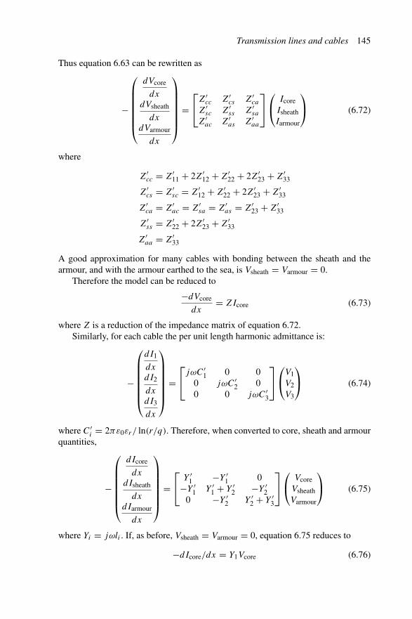
Transmission lines and cables 145
Thus equation 6.63 can be rewritten as
−
⎛
⎜⎜⎜⎜⎜⎜⎝
dVcore
dx
dVsheath
dx
dVarmour
dx
⎞
⎟⎟⎟⎟⎟⎟⎠
=⎡
⎣Z′
cc Z′cs Z′
ca
Z′sc Z′
ss Z′sa
Z′ac Z′
as Z′aa
⎤
⎦
⎛
⎝IcoreIsheathIarmour
⎞
⎠ (6.72)
where
Z′cc = Z′
11 + 2Z′12 + Z′
22 + 2Z′23 + Z′
33
Z′cs = Z′
sc = Z′12 + Z′
22 + 2Z′23 + Z′
33
Z′ca = Z′
ac = Z′sa = Z′
as = Z′23 + Z′
33
Z′ss = Z′
22 + 2Z′23 + Z′
33
Z′aa = Z′
33
A good approximation for many cables with bonding between the sheath and thearmour, and with the armour earthed to the sea, is Vsheath = Varmour = 0.
Therefore the model can be reduced to
−dVcore
dx= ZIcore (6.73)
where Z is a reduction of the impedance matrix of equation 6.72.Similarly, for each cable the per unit length harmonic admittance is:
−
⎛
⎜⎜⎜⎜⎜⎜⎝
dI1
dx
dI2
dx
dI3
dx
⎞
⎟⎟⎟⎟⎟⎟⎠
=⎡
⎣jωC′
1 0 00 jωC′
2 00 0 jωC′
3
⎤
⎦
⎛
⎝V1V2V3
⎞
⎠ (6.74)
where C′i = 2πε0εr/ ln(r/q). Therefore, when converted to core, sheath and armour
quantities,
−
⎛
⎜⎜⎜⎜⎜⎜⎝
dIcore
dx
dIsheath
dx
dIarmour
dx
⎞
⎟⎟⎟⎟⎟⎟⎠
=⎡
⎣Y ′
1 −Y ′1 0
−Y ′1 Y ′
1 + Y ′2 −Y ′
20 −Y ′
2 Y ′2 + Y ′
3
⎤
⎦
⎛
⎝VcoreVsheathVarmour
⎞
⎠ (6.75)
where Yi = jωli . If, as before, Vsheath = Varmour = 0, equation 6.75 reduces to
−dIcore/dx = Y1Vcore (6.76)

146 Power systems electromagnetic transients simulation
Therefore, for the frequencies of interest, the cable per unit length impedance, Z′,and admittance, Y ′, are calculated with both the zero and positive sequence valuesbeing equal to the Z in equation 6.73, and the Y1 in equation 6.76, respectively. Inthe absence of rigorous computer models, such as described above, power companiesoften use approximations to the skin effect by means of correction factors.
6.6 Example
To illustrate various transmission line representations let us consider two simple lineswith the parameters shown in Tables 6.1 and 6.2.
For the transmission line with the parameters shown in Table 6.1, γ =0.500000E−08, Zc = 100 � and the line travelling delay is 0.25 ms (or 5 timesteps). This delay can clearly be seen in Figures 6.15 and 6.16. Note also the lack ofreflections when the line is terminated by the characteristic impedance (Figure 6.15).Reflections cause a step change every 0.5 ms, or twice the travelling time.
When the load impedance is larger than the characteristic impedance (Figure 6.16)a magnified voltage at the receiving end (of 33 per cent in this case) appears 0.25 msafter the step occurs at the sending end. This also results in a receiving end currentbeginning to flow at this time. The receiving end voltage and current then propagateback to the sending end, after a time delay of 0.25 ms, altering the sending end current.
Table 6.1 Parameters for transmissionline example
L′ 500 × 10−9 H m−1
C′ 50 × 10−9 F m−1
L 50 kmR (source) 0.1 �
�t 50 μs
Table 6.2 Single phase test transmissionline
Description Value
Ground resistivity (� m) 100.0Line length (km) 100.0Conductor radius (cm) 2.03454Height at tower Y (m) 30.0Sag at mid-span (m) 10.0d.c. resistance (� km−1) 0.03206
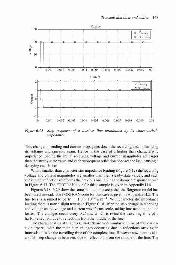
Transmission lines and cables 147
VoltageV
olta
geVSendingVReceiving
Current
Cur
rent
0
50
100
150
–2
–1
0
1
2
0 0.001 0.002 0.003 0.004 0.005 0.006 0.007 0.008 0.009 0.01
0 0.001 0.002 0.003 0.004 0.005 0.006 0.007 0.008 0.009 0.01
ISendingIReceiving
Figure 6.15 Step response of a lossless line terminated by its characteristicimpedance
This change in sending end current propagates down the receiving end, influencingits voltages and currents again. Hence in the case of a higher than characteristicimpedance loading the initial receiving voltage and current magnitudes are largerthan the steady-state value and each subsequent reflection opposes the last, causing adecaying oscillation.
With a smaller than characteristic impedance loading (Figure 6.17) the receivingvoltage and current magnitudes are smaller than their steady-state values, and eachsubsequent reflection reinforces the previous one, giving the damped response shownin Figure 6.17. The FORTRAN code for this example is given in Appendix H.4.
Figures 6.18–6.20 show the same simulation except that the Bergeron model hasbeen used instead. The FORTRAN code for this case is given in Appendix H.5. Theline loss is assumed to be R′ = 1.0 × 10⁻⁴ � m−1. With characteristic impedanceloading there is now a slight transient (Figure 6.18) after the step change in receivingend voltage as the voltage and current waveforms settle, taking into account the linelosses. The changes occur every 0.25 ms, which is twice the travelling time of ahalf-line section, due to reflections from the middle of the line.
The characteristics of Figures 6.18–6.20 are very similar to those of the losslesscounterparts, with the main step changes occurring due to reflections arriving inintervals of twice the travelling time of the complete line. However now there is alsoa small step change in between, due to reflections from the middle of the line. The

148 Power systems electromagnetic transients simulation
VoltageV
olta
ge
VSendingVReceiving
Current
Cur
rent
ISendingIReceiving
0
50
100
150
0 0.001 0.002 0.003 0.004 0.005 0.006 0.007 0.008 0.009 0.01
0 0.001 0.002 0.003 0.004 0.005 0.006 0.007 0.008 0.009 0.01–2
–1
0
1
2
Figure 6.16 Step response of a lossless line with a loading of double characteristicimpedance
voltage drop can be clearly seen, the larger voltage drop occurring when the currentis greater.
To illustrate a frequency-dependent transmission line model a simple single wiretransmission line with no earth wire is used next. The line parameters shown inTable 6.2 are used to obtain the electrical parameters of the line and then curve fittingis performed. There are two main ways of calculating the time convolutions requiredto implement a frequency-dependent transmission line. These are either recursiveconvolutions, which require s-domain fitting, or ARMA using z-domain fitting [13].
Figures 6.21 and 6.23 show the match for the attentuation constant and charac-teristic impedance respectively, while the errors associated with the fit are shown inFigures 6.22 and 6.24. The fitted rational function for the characteristic impedanceis shown in Table 6.3 and the partial fraction expansion of its inverse (characteristicadmittance) in Table 6.4.
The ratio of d.c. impedance (taken as the impedance at the lowest frequency,which is 614.41724 �) over the d.c. value of the fitted function (670.1023) is0.91690065830247, therefore this is multiplied with the residuals (k terms inequation 6.55). To ensure the transmission line exhibits the correct d.c. resistancethe attenuation function must also be scaled. The surge impedance function evaluatedat d.c. is ZC(ω = 0) and Rdc is the line resistance per unit length. Then G′ is calcu-lated from G′ = Rdc/Z
2C(ω = 0) and the constant term of the attenuation function
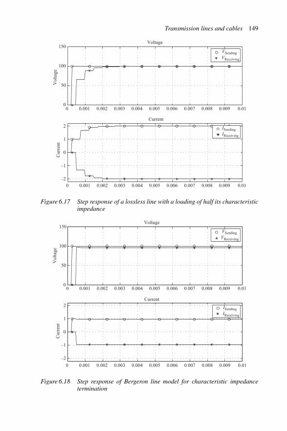
Transmission lines and cables 149
Voltage
Vol
tage
VSending
VReceiving
Current
Cur
rent
ISendingIReceiving
0
50
100
150
0 0.001 0.002 0.003 0.004 0.005 0.006 0.007 0.008 0.009 0.01
–2
–1
0
1
2
0 0.001 0.002 0.003 0.004 0.005 0.006 0.007 0.008 0.009 0.01
Figure 6.17 Step response of a lossless line with a loading of half its characteristicimpedance
0
50
100
150Voltage
Vol
tage
VSending
VReceiving
0 0.001 0.002 0.003 0.004 0.005 0.006 0.007 0.008 0.009 0.01
Current
Cur
rent
ISending
IReceiving
0 0.001 0.002 0.003 0.004 0.005 0.006 0.007 0.008 0.009 0.01
–2
–1
0
1
2
Figure 6.18 Step response of Bergeron line model for characteristic impedancetermination
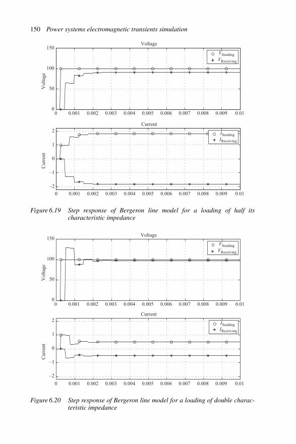
150 Power systems electromagnetic transients simulation
0 0.001 0.002 0.003 0.004 0.005 0.006 0.007 0.008 0.009 0.01
Voltage
VSending
VReceiving
0 0.001 0.002 0.003 0.004 0.005 0.006 0.007 0.008 0.009 0.01
Current
ISendingIReceiving
0
50
100
150
–2
–1
0
1
2
Vol
tage
Cur
rent
Figure 6.19 Step response of Bergeron line model for a loading of half itscharacteristic impedance
VSending
VReceiving
ISendingIReceiving
Voltage
Current
0
50
100
150
–2
–1
0
1
2
Vol
tage
Cur
rent
0 0.001 0.002 0.003 0.004 0.005 0.006 0.007 0.008 0.009 0.01
0 0.001 0.002 0.003 0.004 0.005 0.006 0.007 0.008 0.009 0.01
Figure 6.20 Step response of Bergeron line model for a loading of double charac-teristic impedance

Transmission lines and cables 151
1 2 3 4 5 6 7
Mag
nitu
de
Propagation function
1 2 3 4 5 6 7
Pha
se a
ngle
(de
gs)
log (�)
0
0.2
0.4
0.6
0.8
1
–200
–100
0
100
200
Line constantsFitted function
Figure 6.21 Comparison of attenuation (or propagation) constant
1 2 3 4 5 6 7
Rea
l (er
ror)
Error in propagation function
1 2 3 4 5 6 7
Imag
(er
ror)
–0.1
0
0.1
0.2
0.3
0.4
–0.2
0
0.2
0.4
0.6
Figure 6.22 Error in fitted attenuation constant
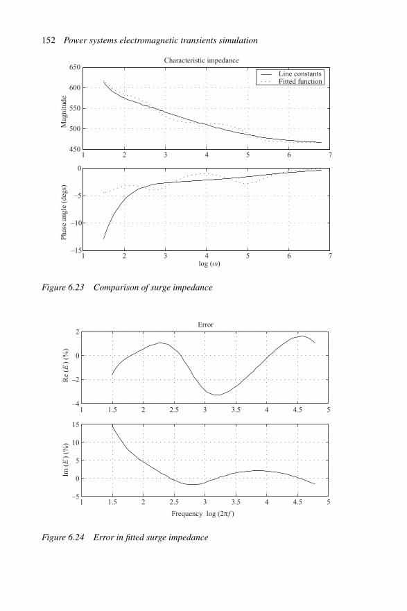
152 Power systems electromagnetic transients simulation
1 2 3 4 5 6 7
Characteristic impedance
Line constantsFitted function
1 2 3 4 5 6 7–15
–10
–5
0
log (�)
450
500
550
600
650M
agni
tude
Pha
se a
ngle
(de
gs)
Figure 6.23 Comparison of surge impedance
Re
(E)
(%)
Im (
E)
(%)
Error
Frequency log (2πf )
–4
–2
0
2
–5
0
5
10
15
1 1.5 2 2.5 3 3.5 4 4.5 5
1 1.5 2 2.5 3 3.5 4 4.5 5
Figure 6.24 Error in fitted surge impedance
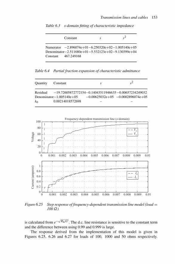
Transmission lines and cables 153
Table 6.3 s-domain fitting of characteristic impedance
Constant s s2
Numerator −2.896074e+01−6.250320e+02−1.005140e+05Denominator−2.511680e+01−5.532123e+02−9.130399e+04Constant 467.249168
Table 6.4 Partial fraction expansion of characteristic admittance
Quantity Constant s s2
Residual −19.72605872772154−0.14043511946635−0.00657234249032Denominator−1.005140e+05 −0.00625032e+05 −0.0002896074e+05k0 0.00214018572698 – –
Frequency-dependent transmission line (s-domain)
Vol
tage
VsVr
0 0.001 0.002 0.003 0.004 0.005 0.006 0.007 0.008 0.009 0.01
Cur
rent
(am
pere
s)
Is–Ir
0
20
40
60
80
100
0
0.2
0.4
0.6
0.8
1
0 0.001 0.002 0.003 0.004 0.005 0.006 0.007 0.008 0.009 0.01
Figure 6.25 Step response of frequency-dependent transmission line model (load =100 Ω)
is calculated from e−√RdcG
′. The d.c. line resistance is sensitive to the constant term
and the difference between using 0.99 and 0.999 is large.The response derived from the implementation of this model is given in
Figures 6.25, 6.26 and 6.27 for loads of 100, 1000 and 50 ohms respectively.
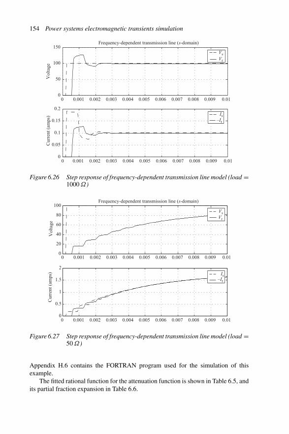
154 Power systems electromagnetic transients simulation
Frequency-dependent transmission line (s-domain)
Vs
Vr
Vol
tage
Cur
rent
(am
ps)
0 0.001 0.002 0.003 0.004 0.005 0.006 0.007 0.008 0.009 0.01
0
50
100
150
0
0.05
0.1
0.15
0.2
0 0.001 0.002 0.003 0.004 0.005 0.006 0.007 0.008 0.009 0.01
Is–Ir
Figure 6.26 Step response of frequency-dependent transmission line model (load =1000 Ω)
0 0.001 0.002 0.003 0.004 0.005 0.006 0.007 0.008 0.009 0.01
Frequency-dependent transmission line (s-domain)
Vol
tage
VsVr
0 0.001 0.002 0.003 0.004 0.005 0.006 0.007 0.008 0.009 0.01
Cur
rent
(am
ps) Is
–Ir
0
20
40
60
80
100
0
0.5
1
1.5
2
Figure 6.27 Step response of frequency-dependent transmission line model (load =50 Ω)
Appendix H.6 contains the FORTRAN program used for the simulation of thisexample.
The fitted rational function for the attenuation function is shown in Table 6.5, andits partial fraction expansion in Table 6.6.
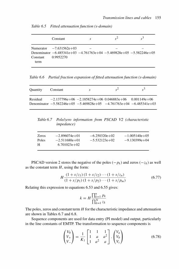
Transmission lines and cables 155
Table 6.5 Fitted attenuation function (s-domain)
Constant s s2 s3
Numerator −7.631562e+03 – – –Denominator −6.485341e+03 −4.761763e+04 −5.469828e+05 −5.582246e+05Constant 0.9952270
term
Table 6.6 Partial fraction expansion of fitted attenuation function (s-domain)
Quantity Constant s s2 s3
Residual −2.137796e+06 −2.1858274e+06 0.046883e+06 0.001149e+06Denominator −5.582246e+05 −5.469828e+05 −4.761763e+04 −6.485341e+03
Table 6.7 Pole/zero information from PSCAD V2 (characteristicimpedance)
Zeros −2.896074e+01 −6.250320e+02 −1.005140e+05Poles −2.511680e+01 −5.532123e+02 −9.130399e+04H 6.701023e+02
PSCAD version 2 stores the negative of the poles (−pk) and zeros (−zk) as wellas the constant term H , using the form:
H(1 + s/z1) (1 + s/z2) · · · (1 + s/zn)
(1 + s/p1) (1 + s/p2) · · · (1 + s/pm)(6.77)
Relating this expression to equations 6.53 and 6.55 gives:
k = H
∏nk=1 pk
∏Nk=1 zk
The poles, zeros and constant term H for the characteristic impedance and attenuationare shown in Tables 6.7 and 6.8.
Sequence components are used for data entry (PI model) and output, particularlyin the line constants of EMTP. The transformation to sequence components is
⎛
⎝V0V+V−
⎞
⎠ = 1
K1
⎡
⎣1 1 11 a a2
1 a2 a
⎤
⎦ .
⎛
⎝Va
Vb
Vc
⎞
⎠ (6.78)

156 Power systems electromagnetic transients simulation
Table 6.8 Pole/zero information from PSCAD V2 (attenuationfunction)
Zeros−7.631562e+03Poles−6.485341e+03−4.761763e+04−5.469828e+05−5.582246e+05H 9.952270e−01
and the reverse transform:⎛
⎝Va
Vb
Vc
⎞
⎠ = 1
K2
⎡
⎣1 1 11 a2 a
1 a a2
⎤
⎦ .
⎛
⎝V0V+V−
⎞
⎠
where a = ej120 = −1/2 + j√
3/2.The power industry uses values of K1 = 3 and K2 = 1, but in the normalised
version both K1 and K2 are equal to√
3. Although the choice of factors affect thesequence voltages and currents, the sequence impedances are unaffected by them.
6.7 Summary
For all except very short transmission lines, travelling wave transmission line modelsare preferable. If frequency dependence is important then a frequency transmissionline dependent model will be used. Details of transmission line geometry and conduc-tor data are then required in order to calculate accurately the frequency-dependentelectrical parameters of the line. The simulation time step must be based on theshortest response time of the line.
Many variants of frequency-dependent multiconductor transmission line modelsexist. A widely used model is based on ignoring the frequency dependence of thetransformation matrix between phase and mode domains (i.e. the J. Marti model inEMTP [14]).
At present phase-domain models are the most accurate and robust for detailedtransmission line representation. Given the complexity and variety of undergroundcables, a rigorous unified solution similar to that of the overhead line is only possiblebased on a standard cross-section structure and under various simplifying assump-tions. Instead, power companies often use correction factors, based on experience,for skin effect representation.
6.8 References
1 CARSON, J. R.: ‘Wave propagation in overhead wires with ground return’, BellSystem Technical Journal, 1926, 5, pp. 539–54
Transmission lines and cables 157
2 POLLACZEK, F.: ‘On the field produced by an infinitely long wire carryingalternating current’, Elektrische Nachrichtentechnik, 1926, 3, pp. 339–59
3 POLLACZEK, F.: ‘On the induction effects of a single phase ac line’, ElektrischeNachrichtentechnik, 1927, 4, pp. 18–30
4 GUSTAVSEN, B. and SEMLYEN, A.: ‘Simulation of transmission line tran-sients using vector fitting and modal decomposition’, IEEE Transactions on PowerDelivery, 1998, 13 (2), pp. 605–14
5 BERGERON, L.: ‘Du coup de Belier en hydraulique au coup de foudre en elec-tricite’ (Dunod, 1949). (English translation: ‘Water hammer in hydraulics andwave surges in electricity’, ASME Committee, Wiley, New York, 1961.)
6 WEDEPOHL, L. M., NGUYEN, H. V. and IRWIN, G. D.: ‘Frequency-dependent transformation matrices for untransposed transmission lines usingNewton-Raphson method’, IEEE Transactions on Power Systems, 1996, 11 (3),pp. 1538–46
7 CLARKE, E.: ‘Circuit analysis of AC systems, symmetrical and relatedcomponents’ (General Electric Co., Schenectady, NY, 1950)
8 SEMLYEN, A. and DABULEANU, A.: ‘Fast and accurate switching transient cal-culations on transmission lines with ground return using recursive convolutions’,IEEE Transactions on Power Apparatus and Systems, 1975, 94 (2), pp. 561–71
9 SEMLYEN, A.: ‘Contributions to the theory of calculation of electromagnetictransients on transmission lines with frequency dependent parameters’, IEEETransactions on Power Apparatus and Systems, 1981, 100 (2), pp. 848–56
10 MORCHED, A., GUSTAVSEN, B. and TARTIBI, M.: ‘A universal modelfor accurate calculation of electromagnetic transients on overhead lines andunderground cables’, IEEE Transactions on Power Delivery, 1999, 14 (3),pp. 1032–8
11 DERI, A., TEVAN, G., SEMLYEN, A. and CASTANHEIRA, A.: ‘The complexground return plane, a simplified model for homogenous and multi-layer earthreturn’, IEEE Transactions on Power Apparatus and Systems, 1981, 100 (8),pp. 3686–93
12 BIANCHI, G. and LUONI, G.: ‘Induced currents and losses in single-core sub-marine cables’, IEEE Transactions on Power Apparatus and Systems, 1976, 95,pp. 49–58
13 NODA, T.: ‘Development of a transmission-line model considering the skinand corona effects for power systems transient analysis’ (Ph.D. thesis, DoshishaUniversity, Kyoto, Japan, December 1996)
14 MARTI, J. R.: ‘Accurate modelling of frequency-dependent transmission lines inelectromagnetic transient simulations’, IEEE Transactions on Power Apparatusand Systems, 1982, 101 (1), pp. 147–57

Chapter 7
Transformers and rotating plant
7.1 Introduction
The simulation of electrical machines, whether static or rotative, requires anunderstanding of the electromagnetic characteristics of their respective windings andcores. Due to their basically symmetrical design, rotating machines are simpler in thisrespect. On the other hand the latter’s transient behaviour involves electromechani-cal as well as electromagnetic interactions. Electrical machines are discussed in thischapter with emphasis on their magnetic properties. The effects of winding capaci-tances are generally negligible for studies other than those involving fast fronts (suchas lightning and switching).
The first part of the chapter describes the dynamic behaviour and computer sim-ulation of single-phase, multiphase and multilimb transformers, including saturationeffects [1]. Early models used with electromagnetic transient programs assumed auniform flux throughout the core legs and yokes, the individual winding leakageswere combined and the magnetising current was placed on one side of the resultantseries leakage reactance. An advanced multilimb transformer model is also described,based on unified magnetic equivalent circuit recently implemented in the EMTDCprogram.
In the second part, the chapter develops a general dynamic model of the rotatingmachine, with emphasis on the synchronous generator. The model includes an accu-rate representation of the electrical generator behaviour as well as the mechanicalcharacteristics of the generator and the turbine. In most cases the speed variationsand torsional vibrations can be ignored and the mechanical part can be left out of thesimulation.

160 Power systems electromagnetic transients simulation
7.2 Basic transformer model
The equivalent circuit of the basic transformer model, shown in Figure 7.1, consistsof two mutually coupled coils. The voltages across these coils is expressed as:
(v1v2
)=
[L11 L21L12 L22
]d
dt
(i1i2
)(7.1)
where L11 and L22 are the self-inductance of winding 1 and 2 respectively, and L12and L21 are the mutual inductance between the windings.
In order to solve for the winding currents the inductance matrix has to beinverted, i.e.
d
dt
(i1i2
)= 1
L11L22 − L12L21
[L22 −L21
−L12 L11
](v1v2
)(7.2)
Since the mutual coupling is bilateral, L12 and L21 are identical. The couplingcoefficient between the two coils is:
K12 = L12√L11L22
(7.3)
Rewriting equation 7.1 using the turns ratio (a = v1/v2) gives:(
v1av2
)=
[L11 L21
aL12 a2L22
]d
dt
(i1
i2/a
)(7.4)
This equation can be represented by the equivalent circuit shown in Figure 7.2,where
L1 = L11 − a L12 (7.5)
L2 = a2L22 − aL12 (7.6)
Consider a transformer with a 10% leakage reactance equally divided betweenthe two windings and a magnetising current of 0.01 p.u. Then the input impedancewith the second winding open circuited must be 100 p.u. (Note from equation 7.5,
av2
i1 L1 L2
aL12
R1 R2 ai2 i2
v1 v2
Idealtransformer
a : 1
Figure 7.1 Equivalent circuit of the two-winding transformer
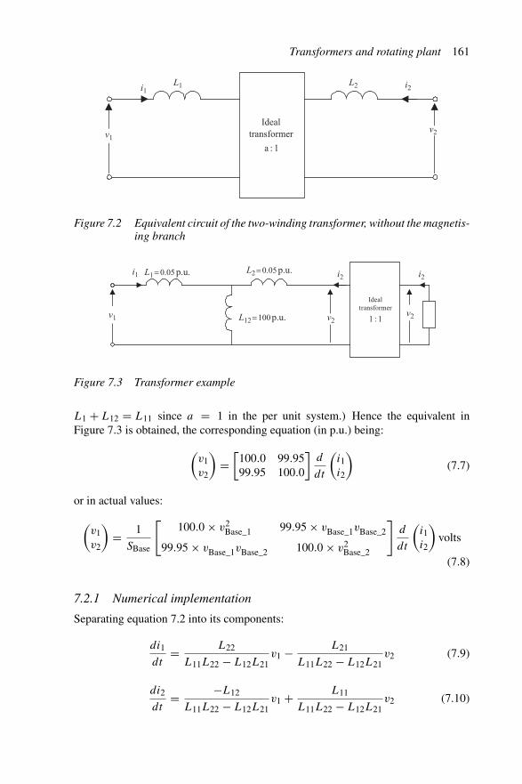
Transformers and rotating plant 161
Idealtransformer
a : 1
v2v1
i1L1 L2 i2
Figure 7.2 Equivalent circuit of the two-winding transformer, without the magnetis-ing branch
Ideal transformer
1 : 1
i1 i2 i2L1 = 0.05 p.u. L2 = 0.05 p.u.
L12 = 100 p.u. v2v1 v2
Figure 7.3 Transformer example
L1 + L12 = L11 since a = 1 in the per unit system.) Hence the equivalent inFigure 7.3 is obtained, the corresponding equation (in p.u.) being:
(v1v2
)=
[100.0 99.9599.95 100.0
]d
dt
(i1i2
)(7.7)
or in actual values:
(v1v2
)= 1
SBase
[100.0 × v2
Base_1 99.95 × vBase_1vBase_2
99.95 × vBase_1vBase_2 100.0 × v2Base_2
]d
dt
(i1i2
)volts
(7.8)
7.2.1 Numerical implementation
Separating equation 7.2 into its components:
di1
dt= L22
L11L22 − L12L21v1 − L21
L11L22 − L12L21v2 (7.9)
di2
dt= −L12
L11L22 − L12L21v1 + L11
L11L22 − L12L21v2 (7.10)
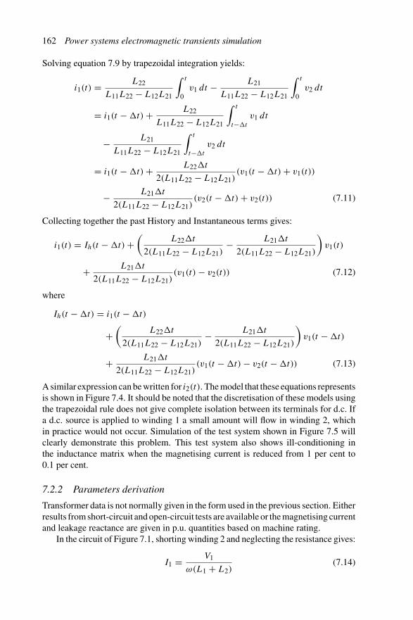
162 Power systems electromagnetic transients simulation
Solving equation 7.9 by trapezoidal integration yields:
i1(t) = L22
L11L22 − L12L21
∫ t
0v1 dt − L21
L11L22 − L12L21
∫ t
0v2 dt
= i1(t − �t) + L22
L11L22 − L12L21
∫ t
t−�t
v1 dt
− L21
L11L22 − L12L21
∫ t
t−�t
v2 dt
= i1(t − �t) + L22�t
2(L11L22 − L12L21)(v1(t − �t) + v1(t))
− L21�t
2(L11L22 − L12L21)(v2(t − �t) + v2(t)) (7.11)
Collecting together the past History and Instantaneous terms gives:
i1(t) = Ih(t − �t) +(
L22�t
2(L11L22 − L12L21)− L21�t
2(L11L22 − L12L21)
)v1(t)
+ L21�t
2(L11L22 − L12L21)(v1(t) − v2(t)) (7.12)
where
Ih(t − �t) = i1(t − �t)
+(
L22�t
2(L11L22 − L12L21)− L21�t
2(L11L22 − L12L21)
)v1(t − �t)
+ L21�t
2(L11L22 − L12L21)(v1(t − �t) − v2(t − �t)) (7.13)
A similar expression can be written for i2(t). The model that these equations representsis shown in Figure 7.4. It should be noted that the discretisation of these models usingthe trapezoidal rule does not give complete isolation between its terminals for d.c. Ifa d.c. source is applied to winding 1 a small amount will flow in winding 2, whichin practice would not occur. Simulation of the test system shown in Figure 7.5 willclearly demonstrate this problem. This test system also shows ill-conditioning inthe inductance matrix when the magnetising current is reduced from 1 per cent to0.1 per cent.
7.2.2 Parameters derivation
Transformer data is not normally given in the form used in the previous section. Eitherresults from short-circuit and open-circuit tests are available or the magnetising currentand leakage reactance are given in p.u. quantities based on machine rating.
In the circuit of Figure 7.1, shorting winding 2 and neglecting the resistance gives:
I1 = V1
ω(L1 + L2)(7.14)

Transformers and rotating plant 163
2(Lkk Lmm – Lkm Lmk)
ΔtLmk
2(Lkk Lmm – Lkm Lmk)
Δt (Lmm – Lmk)
2(Lkk Lmm – Lkm Lmk )
Δt (Lkk – Lmk)
Im (t – Δt)Ik (t – Δt)
Figure 7.4 Transformer equivalent after discretisation
L = 0.1 H
R = 1000 Ω110 kV 110 kV110 kV
Leakage = 0.1 p.u.
Figure 7.5 Transformer test system
Similarly, open-circuit tests with windings 2 or 1 open-circuited, respectively give:
I1 = V1
ω(L1 + aL12)(7.15)
I2 = a2V2
ω(L2 + aL12)(7.16)
Short and open circuit tests provide enough information to determineaL12, L1 andL2.These calculations are often performed internally in the transient simulation program,and the user only needs to enter directly the leakage and magnetising reactances.
The inductance matrix contains information to derive the magnetising currentand also, indirectly through the small differences between L11 and L12, the leakage(short-circuit) reactance.
The leakage reactance is given by:
LLeakage = L11 − L221/L22 (7.17)
In most studies the leakage reactance has the greatest influence on the results. Thus thevalues of the inductance matrix must be specified very accurately to reduce errors dueto loss of significance caused by subtracting two numbers of very similar magnitude.
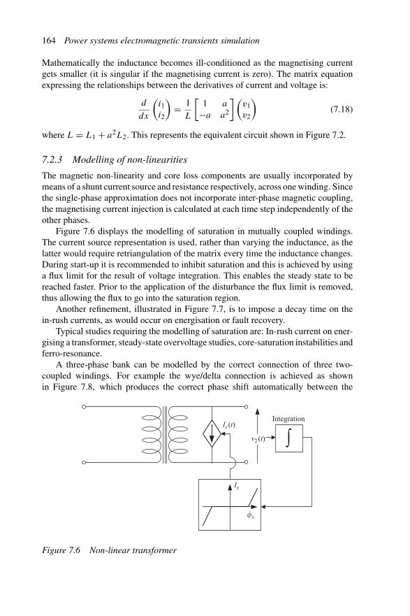
164 Power systems electromagnetic transients simulation
Mathematically the inductance becomes ill-conditioned as the magnetising currentgets smaller (it is singular if the magnetising current is zero). The matrix equationexpressing the relationships between the derivatives of current and voltage is:
d
dx
(i1i2
)= 1
L
[1 a
−a a2
](v1v2
)(7.18)
where L = L1 + a2L2. This represents the equivalent circuit shown in Figure 7.2.
7.2.3 Modelling of non-linearities
The magnetic non-linearity and core loss components are usually incorporated bymeans of a shunt current source and resistance respectively, across one winding. Sincethe single-phase approximation does not incorporate inter-phase magnetic coupling,the magnetising current injection is calculated at each time step independently of theother phases.
Figure 7.6 displays the modelling of saturation in mutually coupled windings.The current source representation is used, rather than varying the inductance, as thelatter would require retriangulation of the matrix every time the inductance changes.During start-up it is recommended to inhibit saturation and this is achieved by usinga flux limit for the result of voltage integration. This enables the steady state to bereached faster. Prior to the application of the disturbance the flux limit is removed,thus allowing the flux to go into the saturation region.
Another refinement, illustrated in Figure 7.7, is to impose a decay time on thein-rush currents, as would occur on energisation or fault recovery.
Typical studies requiring the modelling of saturation are: In-rush current on ener-gising a transformer, steady-state overvoltage studies, core-saturation instabilities andferro-resonance.
A three-phase bank can be modelled by the correct connection of three two-coupled windings. For example the wye/delta connection is achieved as shownin Figure 7.8, which produces the correct phase shift automatically between the
�s
Is
Integration
Is (t)
v2 (t) ∫
Figure 7.6 Non-linear transformer

Transformers and rotating plant 165
�s
Is
Integration
Is (t)
v2 (t) +– ∫
2TDecay
1
Figure 7.7 Non-linear transformer model with in-rush
LB
LA
HB
HA
HC
LC
Figure 7.8 Star–delta three-phase transformer
primary and secondary windings (secondary lagging primary by 30 degrees in thecase shown) [2].
7.3 Advanced transformer models
To take into account the magnetising currents and core configuration of multilimbtransformers the EMTP package has developed a program based on the principle
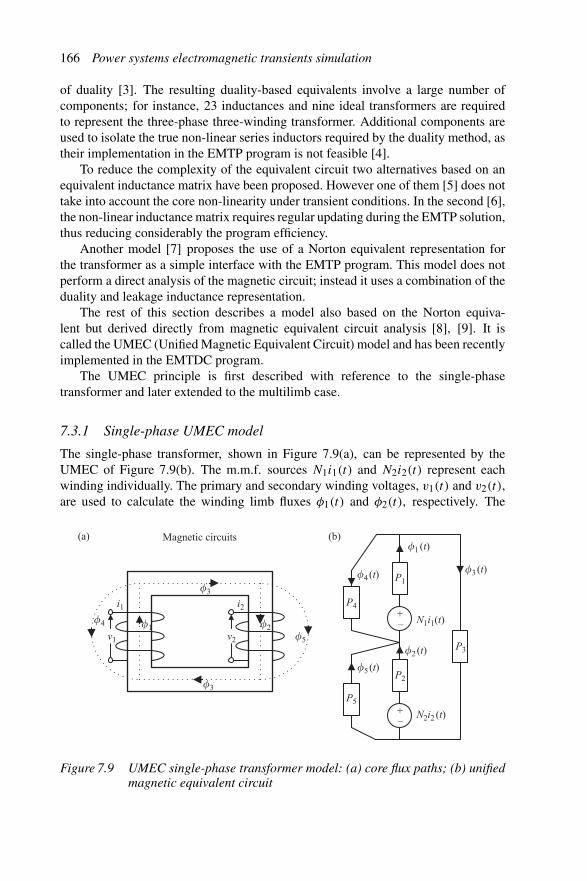
166 Power systems electromagnetic transients simulation
of duality [3]. The resulting duality-based equivalents involve a large number ofcomponents; for instance, 23 inductances and nine ideal transformers are requiredto represent the three-phase three-winding transformer. Additional components areused to isolate the true non-linear series inductors required by the duality method, astheir implementation in the EMTP program is not feasible [4].
To reduce the complexity of the equivalent circuit two alternatives based on anequivalent inductance matrix have been proposed. However one of them [5] does nottake into account the core non-linearity under transient conditions. In the second [6],the non-linear inductance matrix requires regular updating during the EMTP solution,thus reducing considerably the program efficiency.
Another model [7] proposes the use of a Norton equivalent representation forthe transformer as a simple interface with the EMTP program. This model does notperform a direct analysis of the magnetic circuit; instead it uses a combination of theduality and leakage inductance representation.
The rest of this section describes a model also based on the Norton equiva-lent but derived directly from magnetic equivalent circuit analysis [8], [9]. It iscalled the UMEC (Unified Magnetic Equivalent Circuit) model and has been recentlyimplemented in the EMTDC program.
The UMEC principle is first described with reference to the single-phasetransformer and later extended to the multilimb case.
7.3.1 Single-phase UMEC model
The single-phase transformer, shown in Figure 7.9(a), can be represented by theUMEC of Figure 7.9(b). The m.m.f. sources N1i1(t) and N2i2(t) represent eachwinding individually. The primary and secondary winding voltages, v1(t) and v2(t),are used to calculate the winding limb fluxes φ1(t) and φ2(t), respectively. The
i1�4
�3
�3
�2�5
�4 (t)
�1 (t)
�3 (t)
�2 (t)
�5 (t)
N1i1(t)
N2i2 (t)
�1v1 v2
i2 P4
P5
P2
P1
P3
–+
–+
Magnetic circuits(a) (b)
Figure 7.9 UMEC single-phase transformer model: (a) core flux paths; (b) unifiedmagnetic equivalent circuit
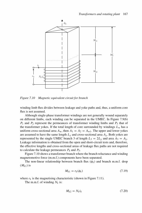
Transformers and rotating plant 167
�k
Mk1
Mk2
Nk ikvk
ik
M�k
Figure 7.10 Magnetic equivalent circuit for branch
winding limb flux divides between leakage and yoke paths and, thus, a uniform coreflux is not assumed.
Although single-phase transformer windings are not generally wound separatelyon different limbs, each winding can be separated in the UMEC. In Figure 7.9(b)P1 and P2 represent the permeances of transformer winding limbs and P3 that ofthe transformer yokes. If the total length of core surrounded by windings Lw has auniform cross-sectional area Aw, then A1 = A2 = Aw1. The upper and lower yokesare assumed to have the same length Ly and cross-sectional area Ay. Both yokes arerepresented by the single UMEC branch 3 of length L3 = 2Ly and area A3 = Ay.Leakage information is obtained from the open and short-circuit tests and, therefore,the effective lengths and cross-sectional areas of leakage flux paths are not requiredto calculate the leakage permeances P4 and P5.
Figure 7.10 shows a transformer branch where the branch reluctance and windingmagnetomotive force (m.m.f.) components have been separated.
The non-linear relationship between branch flux (φk) and branch m.m.f. drop(Mk1) is
Mk1 = rk(φk) (7.19)
where rk is the magnetising characteristic (shown in Figure 7.11).The m.m.f. of winding Nk is:
Mk2 = Nkik (7.20)
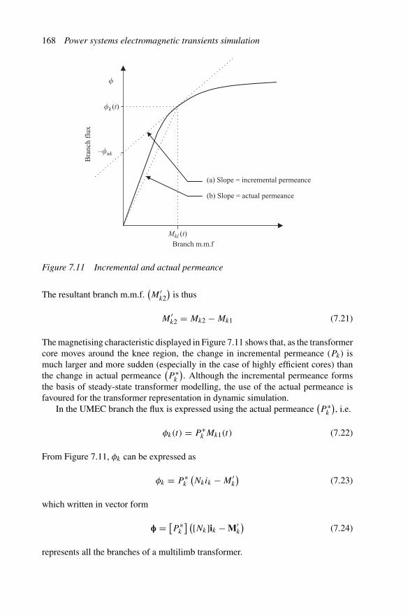
168 Power systems electromagnetic transients simulation
Branch m.m.f
Bra
nch
flux
�
�k (t)
Mkl (t)
–�nk
(a) Slope = incremental permeance
(b) Slope = actual permeance
Figure 7.11 Incremental and actual permeance
The resultant branch m.m.f.(M ′
k2
)is thus
M ′k2 = Mk2 − Mk1 (7.21)
The magnetising characteristic displayed in Figure 7.11 shows that, as the transformercore moves around the knee region, the change in incremental permeance (Pk) ismuch larger and more sudden (especially in the case of highly efficient cores) thanthe change in actual permeance
(P ∗
k
). Although the incremental permeance forms
the basis of steady-state transformer modelling, the use of the actual permeance isfavoured for the transformer representation in dynamic simulation.
In the UMEC branch the flux is expressed using the actual permeance(P ∗
k
), i.e.
φk(t) = P ∗k Mk1(t) (7.22)
From Figure 7.11, φk can be expressed as
φk = P ∗k
(Nkik − M ′
k
)(7.23)
which written in vector form
φ = [P ∗
k
] ([Nk]ik − M′k
)(7.24)
represents all the branches of a multilimb transformer.

Transformers and rotating plant 169
7.3.1.1 UMEC Norton equivalent
The linearised relationship between winding current and branch flux can be extendedto incorporate the magnetic equivalent-circuit branch connections. Let the node–branch connection matrix of the magnetic circuit be [A] and the vector of nodalmagnetic drops φNode. At each node the flux must sum to zero, i.e.
[A]φNode = 0 (7.25)
Application of the branch–node connection matrix to the vector of nodal magneticdrops gives the branch m.m.f.
[A]MNode = M′ (7.26)
Combining equations 7.24, 7.25 and 7.26 finally yields:
φ = [Q∗][P ∗][N ]i (7.27)
where
[Q∗] = [I ] − [P ∗][A]([A]T [P ∗][A]
)−1 [A]T (7.28)
The winding voltage vk is related to the branch flux φk by:
vk = Nk
dφk
dt(7.29)
Using the trapezoidal integration rule to discretise equation 7.29 gives:
φs(t) = φs(t − �t) + �t
2[Ns]−1(vs(t) + vs(t − �t)) (7.30)
where
φs(t − �t) = φs(t − 2�t) + �t
2[Ns]−1(vs(t − �t) + vs(t − 2�t)) (7.31)
Partitioning the vector of branch flux φ into branches associated with eachtransformer winding φs and using equation 7.30 leads to the Norton equivalent:
is(t) = [Y ∗
ss
]vs(t) + i∗ns(t) (7.32)
where[Y ∗
ss
] = ([Q∗
ss
] [P ∗
s
] [Ns])−1 �t
2[Ns]−1 (7.33)
and
i∗ns(t) = ([Q∗
ss
] [P ∗
s
] [Ns])−1
(�t
2[Ns]−1vs(t − �t) + φ(t − �t)
)(7.34)
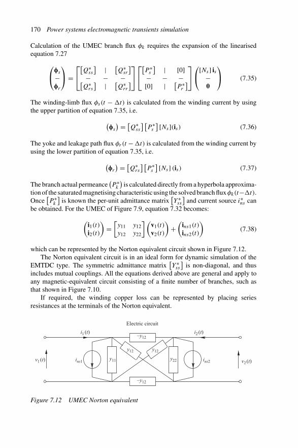
170 Power systems electromagnetic transients simulation
Calculation of the UMEC branch flux φk requires the expansion of the linearisedequation 7.27
⎛
⎝φs
−φr
⎞
⎠ =⎡
⎣
[Q∗
ss
] | [Q∗
sr
]
− − −[Q∗
rs
] | [Q∗
rr
]
⎤
⎦
⎡
⎣
[P ∗
s
] | [0]− − −[0] | [
P ∗r
]
⎤
⎦
⎛
⎝[Ns] is
−0
⎞
⎠ (7.35)
The winding-limb flux φs(t − �t) is calculated from the winding current by usingthe upper partition of equation 7.35, i.e.
(φs
) = [Q∗
ss
] [P ∗
s
] [Ns](is) (7.36)
The yoke and leakage path flux φr(t − �t) is calculated from the winding current byusing the lower partition of equation 7.35, i.e.
(φr
) = [Q∗
rs
] [P ∗
s
] [Ns] (is) (7.37)
The branch actual permeance(P ∗
k
)is calculated directly from a hyperbola approxima-
tion of the saturated magnetising characteristic using the solved branch fluxφk(t−�t).Once
[P ∗
k
]is known the per-unit admittance matrix
[Y ∗
ss
]and current source i∗ns can
be obtained. For the UMEC of Figure 7.9, equation 7.32 becomes:
(i1(t)i2(t)
)=
[y11 y12y12 y22
](v1(t)
v2(t)
)+
(ins1(t)
ins2(t)
)(7.38)
which can be represented by the Norton equivalent circuit shown in Figure 7.12.The Norton equivalent circuit is in an ideal form for dynamic simulation of the
EMTDC type. The symmetric admittance matrix[Y ∗
ss
]is non-diagonal, and thus
includes mutual couplings. All the equations derived above are general and apply toany magnetic-equivalent circuit consisting of a finite number of branches, such asthat shown in Figure 7.10.
If required, the winding copper loss can be represented by placing seriesresistances at the terminals of the Norton equivalent.
Electric circuit
v1 (t) ins1 ins2
i1 (t) i2 (t)
v2 (t)y11 y22
y12 y12
–y12
–y12
Figure 7.12 UMEC Norton equivalent
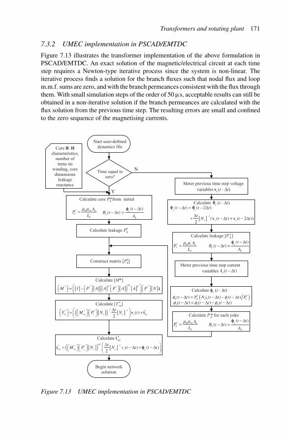
Transformers and rotating plant 171
7.3.2 UMEC implementation in PSCAD/EMTDC
Figure 7.13 illustrates the transformer implementation of the above formulation inPSCAD/EMTDC. An exact solution of the magnetic/electrical circuit at each timestep requires a Newton-type iterative process since the system is non-linear. Theiterative process finds a solution for the branch fluxes such that nodal flux and loopm.m.f. sums are zero, and with the branch permeances consistent with the flux throughthem. With small simulation steps of the order of 50 μs, acceptable results can still beobtained in a non-iterative solution if the branch permeances are calculated with theflux solution from the previous time step. The resulting errors are small and confinedto the zero sequence of the magnetising currents.
Y
N
Figure 7.13 UMEC implementation in PSCAD/EMTDC

172 Power systems electromagnetic transients simulation
The leakage-flux branch permeances are constant and the core branch-saturationcharacteristic is the steel flux density magnetising force (B–H) curve. Individualbranch per unitφ−i characteristics are not a conventional specification but, if required,these can be provided by the manufacturer.
Core dimensions, branch length Lk and cross-sectional area Ak , are required tocalculate real value permeances from
P ∗k = μ0μrkAk
Lk
(7.39)
The branch flux φk(t − �t) is converted to branch flux density by
Bk(t − �t) = φk(t − �t)
Ak
(7.40)
The branch permeability μ0μrk is then calculated from the core B–H characteristic.Figure 7.13 also shows that the winding-limb flux φs(t − �t) is calculated using
trapezoidal integration rather than the linearised equation 7.27. Trapezoidal integra-tion requires storage of vectors φs(t−2�t) and vs(t−2�t). In equation 7.27 matrices[Q∗
ss
]and
[P ∗
ss
]must be stored and, although
[P ∗
ss
]is diagonal,
[Q∗
ss
]is full; therefore
in this method element storage increases with the square of the UMEC winding-limbbranch number.
The elements of φr(t − �t) can be calculated using magnetic circuit theory,whereby the m.m.f. around the primary winding limb and leakage branch loop mustsum to zero, i.e. with reference to Figure 7.9(b),
φ4(t − �t) = P ∗4
(N1i1(t − �t) − φ1(t − �t)/P ∗
1
)(7.41)
Also, the m.m.f. around the secondary winding limb and leakage branch loop mustsum to zero
φ5(t − �t) = P ∗5
(N2i2(t − �t) − φ2(t − �t)/P ∗
2
)(7.42)
and, finally, the flux at node N1 must sum to zero:
φ3(t − �t) = φ1(t − �t)) − φ4(t − �t) (7.43)
The yoke branch actual permeance P ∗k is calculated directly from the solved branch
flux φk(t − �t) using equations 7.39 and 7.40. Once [P ∗] is known, the real-valuedadmittance matrix
[Y ∗
ss
]and current source vector i∗ns can be obtained.
7.3.3 Three-limb three-phase UMEC
An extension of the single-phase UMEC concept to the three-phase transformer,shown in Figure 7.14(a), leads to the UMEC of Figure 7.14(b). There is no needto specify in advance the distribution of magnetising current components, whichhave been shown to be determined by the transformer internal and external circuitparameters.
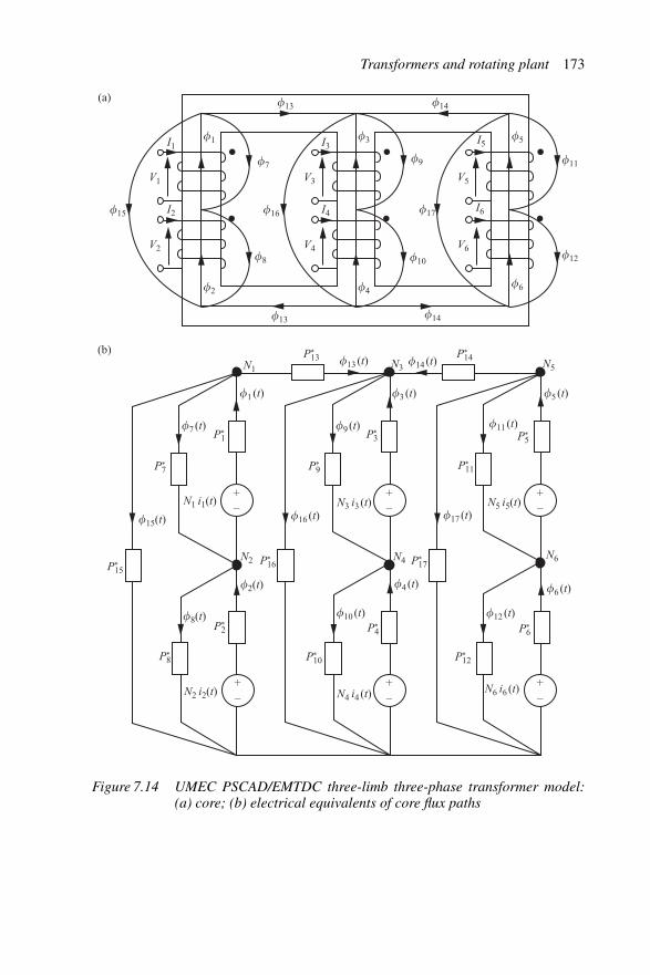
Transformers and rotating plant 173
I1
I2
V1
V2
�1
�2
�8
�16 �17
�10
�14
�9
�13
�13 �14
�15
I3
I4
V3
V4
�3
�4
I5
I6
V5
V6
�5
�6
�12
�11�7
+–
+–
+–
+–
+–
+–
P*15
P*16 P*
17
P*10 P*
12
P*4P*
2
P*7 P*
9
P*1
P*13 P*
14
P*11
P*5
P*6
P*3
�15(t)
�7 (t)
�1 (t) �3 (t) �5 (t)
�6 (t)
�12 (t)
�17 (t)
�9 (t) �11 (t)
�13 (t) �14 (t)
�2(t)
�16 (t)
�10 (t)
�4 (t)
�8(t)
P*8
N1 i1(t) N5 i5(t)
N6 i6 (t)N2 i2(t) N4 i4 (t)
N3 i3 (t)
N2
N1 N3 N5
N6N4
(a)
(b)
Figure 7.14 UMEC PSCAD/EMTDC three-limb three-phase transformer model:(a) core; (b) electrical equivalents of core flux paths
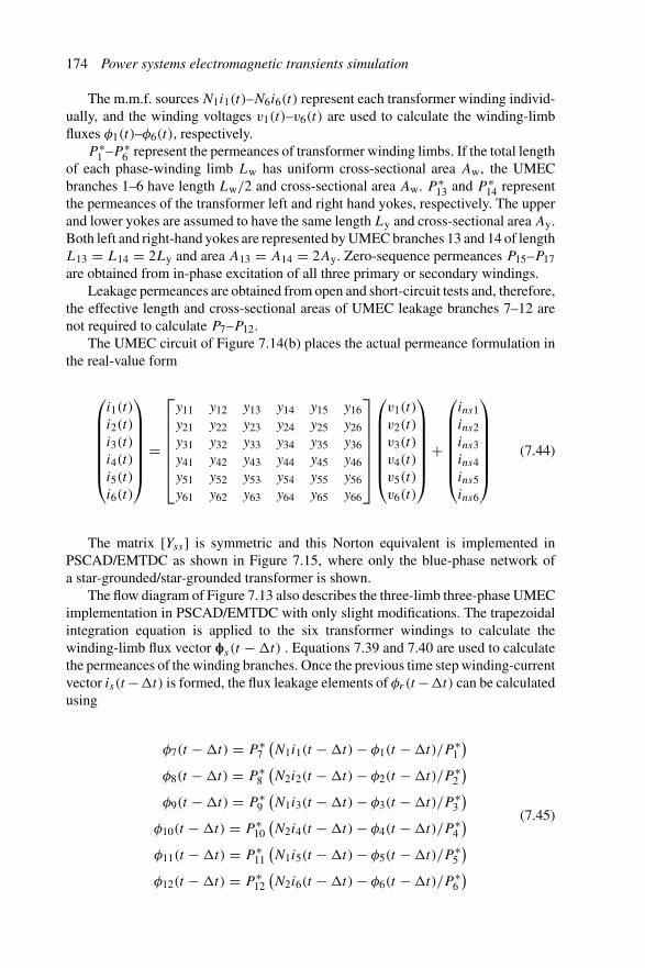
174 Power systems electromagnetic transients simulation
The m.m.f. sources N1i1(t)–N6i6(t) represent each transformer winding individ-ually, and the winding voltages v1(t)–v6(t) are used to calculate the winding-limbfluxes φ1(t)–φ6(t), respectively.
P ∗1 –P ∗
6 represent the permeances of transformer winding limbs. If the total lengthof each phase-winding limb Lw has uniform cross-sectional area Aw, the UMECbranches 1–6 have length Lw/2 and cross-sectional area Aw. P ∗
13 and P ∗14 represent
the permeances of the transformer left and right hand yokes, respectively. The upperand lower yokes are assumed to have the same length Ly and cross-sectional area Ay.Both left and right-hand yokes are represented by UMEC branches 13 and 14 of lengthL13 = L14 = 2Ly and area A13 = A14 = 2Ay. Zero-sequence permeances P15–P17are obtained from in-phase excitation of all three primary or secondary windings.
Leakage permeances are obtained from open and short-circuit tests and, therefore,the effective length and cross-sectional areas of UMEC leakage branches 7–12 arenot required to calculate P7–P12.
The UMEC circuit of Figure 7.14(b) places the actual permeance formulation inthe real-value form
⎛
⎜⎜⎜⎜⎜⎜⎝
i1(t)
i2(t)
i3(t)
i4(t)
i5(t)
i6(t)
⎞
⎟⎟⎟⎟⎟⎟⎠
=
⎡
⎢⎢⎢⎢⎢⎢⎣
y11 y12 y13 y14 y15 y16y21 y22 y23 y24 y25 y26y31 y32 y33 y34 y35 y36y41 y42 y43 y44 y45 y46y51 y52 y53 y54 y55 y56y61 y62 y63 y64 y65 y66
⎤
⎥⎥⎥⎥⎥⎥⎦
⎛
⎜⎜⎜⎜⎜⎜⎝
v1(t)
v2(t)
v3(t)
v4(t)
v5(t)
v6(t)
⎞
⎟⎟⎟⎟⎟⎟⎠
+
⎛
⎜⎜⎜⎜⎜⎜⎝
ins1ins2ins3ins4ins5ins6
⎞
⎟⎟⎟⎟⎟⎟⎠
(7.44)
The matrix [Yss] is symmetric and this Norton equivalent is implemented inPSCAD/EMTDC as shown in Figure 7.15, where only the blue-phase network ofa star-grounded/star-grounded transformer is shown.
The flow diagram of Figure 7.13 also describes the three-limb three-phase UMECimplementation in PSCAD/EMTDC with only slight modifications. The trapezoidalintegration equation is applied to the six transformer windings to calculate thewinding-limb flux vector φs(t − �t) . Equations 7.39 and 7.40 are used to calculatethe permeances of the winding branches. Once the previous time step winding-currentvector is(t −�t) is formed, the flux leakage elements of φr(t −�t) can be calculatedusing
φ7(t − �t) = P ∗7
(N1i1(t − �t) − φ1(t − �t)/P ∗
1
)
φ8(t − �t) = P ∗8
(N2i2(t − �t) − φ2(t − �t)/P ∗
2
)
φ9(t − �t) = P ∗9
(N1i3(t − �t) − φ3(t − �t)/P ∗
3
)
φ10(t − �t) = P ∗10
(N2i4(t − �t) − φ4(t − �t)/P ∗
4
)
φ11(t − �t) = P ∗11
(N1i5(t − �t) − φ5(t − �t)/P ∗
5
)
φ12(t − �t) = P ∗12
(N2i6(t − �t) − φ6(t − �t)/P ∗
6
)
(7.45)
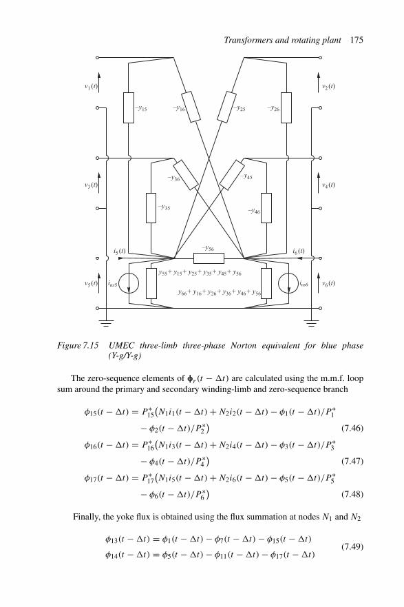
Transformers and rotating plant 175
ins6
v1 (t)
v3 (t)
v5 (t)
v2 (t)
v4 (t)
v6 (t)ins5
i5 (t) i6 (t)
–y15 –y16 –y26
–y36–y45
–y46
–y56
y55 + y15 + y25 + y35 + y45 + y56
y66 + y16 + y26 + y36 + y46 + y56
–y35
–y25
Figure 7.15 UMEC three-limb three-phase Norton equivalent for blue phase(Y-g/Y-g)
The zero-sequence elements of φr (t − �t) are calculated using the m.m.f. loopsum around the primary and secondary winding-limb and zero-sequence branch
φ15(t − �t) = P ∗15
(N1i1(t − �t) + N2i2(t − �t) − φ1(t − �t)/P ∗
1
− φ2(t − �t)/P ∗2
)(7.46)
φ16(t − �t) = P ∗16
(N1i3(t − �t) + N2i4(t − �t) − φ3(t − �t)/P ∗
3
− φ4(t − �t)/P ∗4
)(7.47)
φ17(t − �t) = P ∗17
(N1i5(t − �t) + N2i6(t − �t) − φ5(t − �t)/P ∗
5
− φ6(t − �t)/P ∗6
)(7.48)
Finally, the yoke flux is obtained using the flux summation at nodes N1 and N2
φ13(t − �t) = φ1(t − �t) − φ7(t − �t) − φ15(t − �t)
φ14(t − �t) = φ5(t − �t) − φ11(t − �t) − φ17(t − �t)(7.49)
176 Power systems electromagnetic transients simulation
The yoke-branch permeances P ∗13 and P ∗
14 are again calculated directly fromsolved branch fluxes φ13 and φ14 using equations 7.39 and 7.40. Once [P ∗] is knownthe real-valued admittance matrix [Y ] can be obtained.
7.3.4 Fast transient models
The inter-turn capacitance is normally ignored at low frequencies, but for high-frequency events this capacitance becomes significant. When subjected to impulsetest the capacitance determines the voltage distribution across the internal windingsof the transformer. Moreover the inter-turn capacitance and winding inductance havea resonant frequency that may be excited. Hence transformer failures can be causedby high-frequency overvoltages due to internal resonances [10], [11]. These internalwinding resonances (typically in the 5–200 kHz range), are initiated by fast tran-sients and may not cause an immediate breakdown, but partial discharges may occur,thereby accelerating ageing of the transformer winding [12]. To determine the voltagelevels across the internal transformer insulation during a specific external transientrequires the use of a detailed high-frequency transformer model. Though the generalhigh-frequency models are very accurate and detailed, they are usually too large tobe incorporated in a general model of the power system [13]. Hence reduced ordermodels, representing the transformer’s terminal behaviour, are normally developedand used in the system study [14]. These reduced order models need to be custommodels developed by the user for the EMTP-type program available. There is a mul-titude of modelling techniques. The resulting transient can be used as the externaltransient into a more detailed high-frequency transformer model, some of which cancalculate down to turn-to-turn voltages.
The difficulty in modelling transformers in detail stems from the fact thatsome transformer parameters are both non-linear and frequency dependent. The ironcore losses and inductances are non-linear due to saturation and hysteresis. Theyare also frequency dependent due to eddy currents in the laminations. During reso-nance phenomena the resistances greatly influence the maximum winding voltages.These resistances represent both the copper and iron losses and are strongly frequencydependent [15]–[17]. Parameters for these models are extracted from laboratory test-ing and are only valid for the transformer type and frequency range of the testsperformed.
7.4 The synchronous machine
The synchronous machine model to be used in each case depends on the time spanof interest. For example the internal e.m.f. behind subtransient reactance is perfectlyadequate for electromagnetic transients studies of only a few cycles, such as the assess-ment of switching oscillations. At the other extreme, transient studies involving speedvariations and/or torsional vibrations need to model adequately the generator rotorand turbine rotor masses. Thus a general-purpose model should include the generatorelectrical parameters as well as the generator and turbine mechanical parameters.
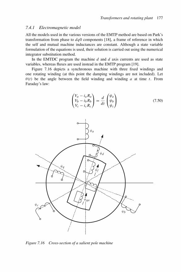
Transformers and rotating plant 177
7.4.1 Electromagnetic model
All the models used in the various versions of the EMTP method are based on Park’stransformation from phase to dq0 components [18], a frame of reference in whichthe self and mutual machine inductances are constant. Although a state variableformulation of the equations is used, their solution is carried out using the numericalintegrator substitution method.
In the EMTDC program the machine d and d axis currents are used as statevariables, whereas fluxes are used instead in the EMTP program [19].
Figure 7.16 depicts a synchronous machine with three fixed windings andone rotating winding (at this point the damping windings are not included). Letθ(t) be the angle between the field winding and winding a at time t . FromFaraday’s law:
⎛
⎝Va − iaRa
Vb − ibRb
Vc − icRc
⎞
⎠ = d
dt
⎛
⎝ψa
ψb
ψc
⎞
⎠ (7.50)
a
d
fq
c
qa
b
Figure 7.16 Cross-section of a salient pole machine
178 Power systems electromagnetic transients simulation
where⎛
⎝ψa
ψb
ψc
⎞
⎠ =⎡
⎣Laa Lab Lac Laf
Lba Lbb Lbc Lbf
Lca Lcb Lcc Lcf
⎤
⎦
⎛
⎜⎜⎝
iaibicif
⎞
⎟⎟⎠
The inductances are of a time varying nature, e.g.
Laa = La + Lm cos(θ)
Lbb = La + Lm cos(2(θ − 2π/3))
Lcc = La + Lm cos(2(θ − 4π/3))
(7.51)
Assuming a sinusoidal winding distribution then the mutual inductances are:
Lab = Lba = −Ms − Lm cos(2(θ − π/6))
Lbc = Lcb = −Ms − Lm cos(2(θ − π/2))
Lca = Lac = −Ms − Lm cos(2(θ + π/2))
(7.52)
and the inductances of the field winding:
Laf = Lf a = Mf cos(θ)
Lbf = Lf b = Mf cos(θ − 2π/3)
Lcf = Lf c = Mf cos(θ − 4π/3)
(7.53)
In compact notation⎛
⎜⎜⎝
ψa
ψb
ψc
ψf
⎞
⎟⎟⎠ =
⎡
⎢⎢⎣
Labc Labcf
Lf abc Lff
⎤
⎥⎥⎦
⎛
⎜⎜⎝
iaibicif
⎞
⎟⎟⎠ (7.54)
or(
ψabc
ψf
)=
[Labc Labcf
Lf abc Lff
](iabc
if
)(7.55)
Taking the top partition
ψabc = [Labc]iabc + [Labcf ]if (7.56)
Choosing a matrix [T (θ)] that diagonalises [Labc] gives:
idq0 = [T (θ)]iabc (7.57)
vdq0 = [T (θ)]vabc (7.58)
ψdq0 = [T (θ)]ψabc (7.59)

Transformers and rotating plant 179
and substituting in equation 7.56 gives
[T (θ)]−1ψdq0 = [Labc][T (θ)]−1idq0 + [Labcf ]if (7.60)
Thusψdq0 = [T (θ)][Labc][T (θ)]−1idq0 + [T (θ)][Labcf ]if
A common choice of [T (θ)] is:
[T (θ)] = 2
3
⎡
⎣cos(θ) cos(θ − 2π/3) cos(θ + 2π/3)
sin(θ) sin(θ − 2π/3) sin(θ + 2π/3)
1/2 1/2 1/2
⎤
⎦ (7.61)
thus
[T (θ)]−1 =⎡
⎣cos(θ) sin(θ) 1
cos(θ − 2π/3) sin(θ − 2π/3) 1cos(θ + 2π/3) sin(θ + 2π/3) 1
⎤
⎦ (7.62)
This matrix is known as Park’s transformation. Therefore the following expressionresults in dq0 coordinates:
⎛
⎝ψd
ψq
ψ0
⎞
⎠ =⎡
⎣La + Ms + 3
2Lm 0 00 La + Ms − 3
2Lm 00 0 La − 2Ms
⎤
⎦
⎛
⎝idiqi0
⎞
⎠+⎛
⎜⎝
√32Mf
00
⎞
⎟⎠
(if)
(7.63)or
⎛
⎝ψd
ψq
ψ0
⎞
⎠ =⎡
⎣La + Lmd 0 0
0 La + Lmd 00 0 L0
⎤
⎦
⎛
⎝idiqi0
⎞
⎠ +⎛
⎝Lmd
00
⎞
⎠(i′f)
(7.64)
whereLmd = Ms + 3
2Lm
i′f =√
3/2Mf
Lmd
if
The equation for the field flux now becomes time dependent, i.e.
(ψf ) = (Mf cos(θ) Mf cos(θ − 2π/3) Mf cos(θ − 4π/3))
×⎡
⎣cos(θ) sin(θ) 1
cos(θ − 2π/3) sin(θ − 2π/3) 1cos(θ + 2π/3) sin(θ + 2π/3) 1
⎤
⎦
⎛
⎝idiqi0
⎞
⎠ + [Lff ] · if
= (32Mf 0 0
)⎛
⎝idiqi0
⎞
⎠ + [Lff ] · if
= 32Mf id + [Lff ] · if (7.65)

180 Power systems electromagnetic transients simulation
id ifLa Lf La
qi
Lmd Lmqdtvd =
dddt
vf =d�f
dtvq =
dq
Figure 7.17 Equivalent circuit for synchronous machine equations
Similarly the field circuit equation can be expressed as:
ψ ′f = [Lmd ]id + [Lmd + Lf ]i′f (7.66)
This can be thought of as transforming the field current to the same base as the statorcurrents. Figure 7.17 depicts the equivalent circuit based on these equations. FromKirchhoff’s current law:
⎛
⎝va − iaRa
vb − ibRb
vc − icRc
⎞
⎠ = d
dt
⎛
⎝ψa
ψb
ψc
⎞
⎠ (7.67)
and
v′f − i′f R′
f = dψ ′f
dt(7.68)
Applying Park’s transformation gives:
[T (θ)]⎛
⎝va − iaRa
vb − ibRb
vc − icRc
⎞
⎠ = [T (θ)] d
dt
⎛
⎝[T (θ)]−1
⎛
⎝ψd
ψq
ψ0
⎞
⎠
⎞
⎠ (7.69)
or
[T (θ)]⎛
⎝vd − idRd
vq − iqRq
v0 − i0R0
⎞
⎠ = [T (θ)]⎛
⎝ d
dt[T (θ)]−1
⎛
⎝ψd
ψq
ψ0
⎞
⎠ + [T (θ)]−1 d
dt
⎛
⎝ψd
ψq
ψ0
⎞
⎠
⎞
⎠
= [T (θ)]⎛
⎝ d
dθ[T (θ)]−1 dθ
dt
⎛
⎝ψd
ψq
ψ0
⎞
⎠ + [T (θ)]−1 d
dt
⎛
⎝ψd
ψq
ψ0
⎞
⎠
⎞
⎠
= [T (θ)] d
dθ[T (θ)]−1ω
⎛
⎝ψd
ψq
ψ0
⎞
⎠
︸ ︷︷ ︸speed emf
+ d
dt
⎛
⎝ψd
ψq
ψ0
⎞
⎠
︸ ︷︷ ︸transformer emf
(7.70)
where ω is the angular speed.
Transformers and rotating plant 181
Evaluating the speed term:
d
dθ[T (θ)]−1 = d
dθ
⎡
⎣cos(θ) sin(θ) 1
cos(θ − 2π/3) sin(θ − 2π/3) 1cos(θ − 4π/3) sin(θ − 4π/3) 1
⎤
⎦ (7.71)
=⎡
⎣− sin(θ) cos(θ) 0
− sin(θ − 2π/3) cos(θ − 2π/3) 0− sin(θ − 4π/3) cos(θ − 4π/3) 0
⎤
⎦ (7.72)
and
[T (θ)] d
dθ[T (θ)]−1 = 2
3
⎡
⎣cos(θ) cos(θ − 2π/3) cos(θ − 4π/3)
sin(θ) sin(θ − 2π/3) sin(θ − 4π/3)
1/2 1/2 1/2
⎤
⎦
×⎡
⎣− sin(θ) cos(θ) 0
− sin(θ − 2π/3) cos(θ − 2π/3) 0− sin(θ − 4π/3) cos(θ − 4π/3) 0
⎤
⎦
= 2
3
⎡
⎣0 2/3 0
−2/3 0 00 0 0
⎤
⎦ =⎡
⎣0 1 0
−1 0 00 0 0
⎤
⎦ (7.73)
Hence equation 7.67 becomes:
vd − idRa = ωψq + dψd
dt
vq − iqRa = −ωψd + dψq
dt
v0 − i0R0 = dψ0
dt
(7.74)
while the field circuit remains unchanged, i.e.
v′f − i′f R′
f = dψ ′f
dt(7.75)
If, as is normally the case, the winding connection is ungrounded star then i0 = 0and the third equation in 7.74 disappears.
Adkins’ [20] equivalent circuit, shown in Figure 7.18, consists of a machine withthree coils on the d-axis and two on the q-axis, although the model can easily be
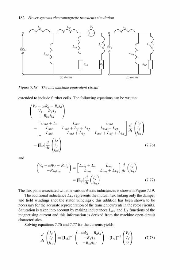
182 Power systems electromagnetic transients simulation
La
Lmd
Lkd
Lmq
Rkd Rkd
Lkq
Rf
Lkf La
Lf
Vf
+ –
dt
dddt
(a) d-axis (b) q-axis
dq
Figure 7.18 The a.c. machine equivalent circuit
extended to include further coils. The following equations can be written:⎛
⎝Vd − ωΨq − Raid
Vf − Rf if−Rkdikd
⎞
⎠
=⎡
⎣Lmd + La Lmd Lmd
Lmd Lmd + Lf + Lkf Lmd + Lkf
Lmd Lmd + Lkf Lmd + Lkf + Lkd
⎤
⎦ d
dt
⎛
⎝idifikd
⎞
⎠
= [Ld ] d
dt
⎛
⎝idifikd
⎞
⎠ (7.76)
and(
Vq + ωΨd − Raiq−Rkqikq
)=
[Lmq + La Lmq
Lmq Lmq + Lkq
]d
dt
(iqikq
)
= [Lq ] d
dt
(iqikq
)(7.77)
The flux paths associated with the various d-axis inductances is shown in Figure 7.19.The additional inductance Lkd represents the mutual flux linking only the damper
and field windings (not the stator windings); this addition has been shown to benecessary for the accurate representation of the transient currents in the rotor circuits.Saturation is taken into account by making inductances Lmd and Lf functions of themagnetising current and this information is derived from the machine open-circuitcharacteristics.
Solving equations 7.76 and 7.77 for the currents yields:
d
dt
⎛
⎝idifikd
⎞
⎠ = [Ld ]−1
⎛
⎝−ωΨd − Raiq
−Rf if−Rkdikd
⎞
⎠ + [Ld ]−1
⎛
⎝Vd
Vf
0
⎞
⎠ (7.78)
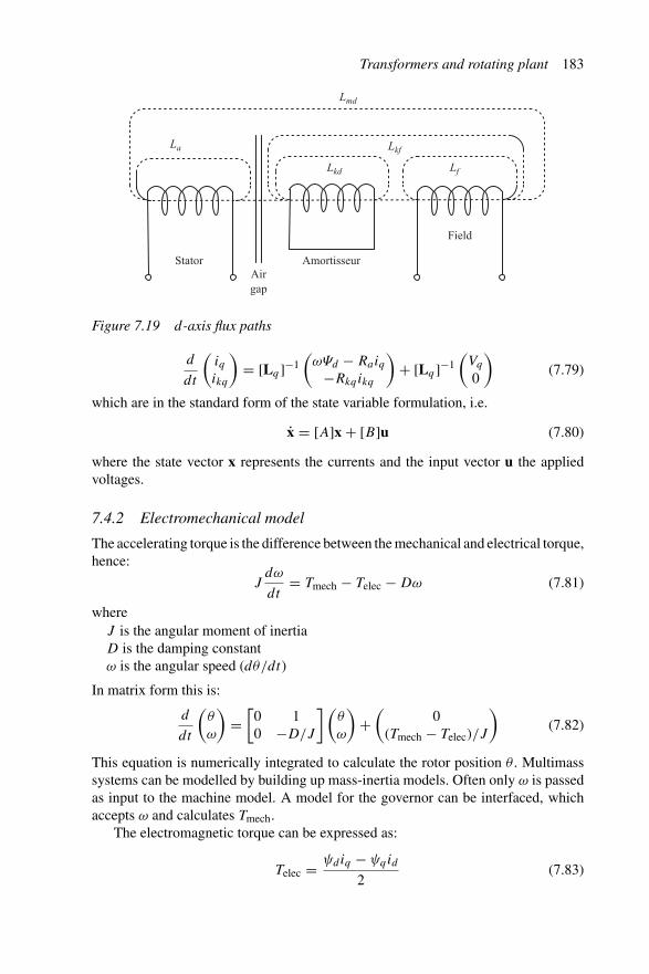
Transformers and rotating plant 183
La Lkf
LfLkd
Lmd
Field
Airgap
AmortisseurStator
Figure 7.19 d-axis flux paths
d
dt
(iqikq
)= [Lq ]−1
(ωΨd − Raiq
−Rkqikq
)+ [Lq ]−1
(Vq
0
)(7.79)
which are in the standard form of the state variable formulation, i.e.
x = [A]x + [B]u (7.80)
where the state vector x represents the currents and the input vector u the appliedvoltages.
7.4.2 Electromechanical model
The accelerating torque is the difference between the mechanical and electrical torque,hence:
Jdω
dt= Tmech − Telec − Dω (7.81)
whereJ is the angular moment of inertiaD is the damping constantω is the angular speed (dθ/dt)
In matrix form this is:
d
dt
(θ
ω
)=
[0 10 −D/J
](θ
ω
)+
(0
(Tmech − Telec)/J
)(7.82)
This equation is numerically integrated to calculate the rotor position θ . Multimasssystems can be modelled by building up mass-inertia models. Often only ω is passedas input to the machine model. A model for the governor can be interfaced, whichaccepts ω and calculates Tmech.
The electromagnetic torque can be expressed as:
Telec = ψdiq − ψqid
2(7.83)
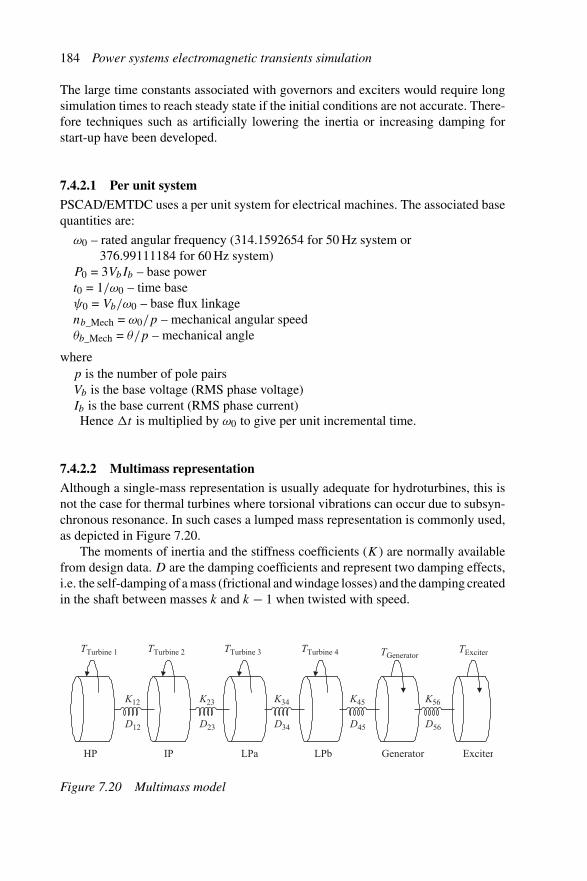
184 Power systems electromagnetic transients simulation
The large time constants associated with governors and exciters would require longsimulation times to reach steady state if the initial conditions are not accurate. There-fore techniques such as artificially lowering the inertia or increasing damping forstart-up have been developed.
7.4.2.1 Per unit system
PSCAD/EMTDC uses a per unit system for electrical machines. The associated basequantities are:
ω0 – rated angular frequency (314.1592654 for 50 Hz system or376.99111184 for 60 Hz system)
P0 = 3VbIb – base powert0 = 1/ω0 – time baseψ0 = Vb/ω0 – base flux linkagenb_Mech = ω0/p – mechanical angular speedθb_Mech = θ/p – mechanical angle
wherep is the number of pole pairsVb is the base voltage (RMS phase voltage)Ib is the base current (RMS phase current)Hence �t is multiplied by ω0 to give per unit incremental time.
7.4.2.2 Multimass representation
Although a single-mass representation is usually adequate for hydroturbines, this isnot the case for thermal turbines where torsional vibrations can occur due to subsyn-chronous resonance. In such cases a lumped mass representation is commonly used,as depicted in Figure 7.20.
The moments of inertia and the stiffness coefficients (K) are normally availablefrom design data. D are the damping coefficients and represent two damping effects,i.e. the self-damping of a mass (frictional and windage losses) and the damping createdin the shaft between masses k and k − 1 when twisted with speed.
TExciterTGeneratorTTurbine 1 TTurbine 2 TTurbine 3 TTurbine 4
D12
K12
D23
K23
D34
K34
D45
K45
D56
K56
HP IP LPa ExciterGeneratorLPb
Figure 7.20 Multimass model
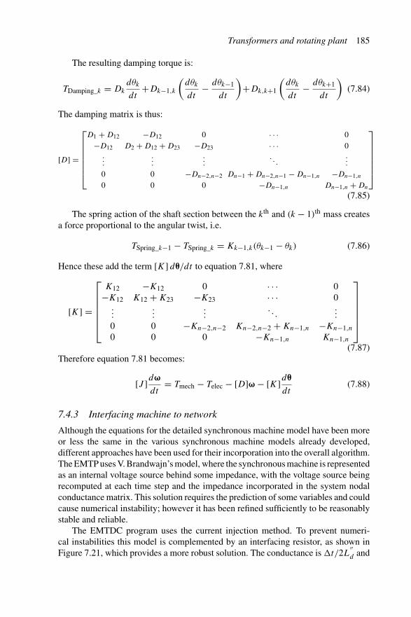
Transformers and rotating plant 185
The resulting damping torque is:
TDamping_k = Dk
dθk
dt+Dk−1,k
(dθk
dt− dθk−1
dt
)+Dk,k+1
(dθk
dt− dθk+1
dt
)(7.84)
The damping matrix is thus:
[D] =
⎡
⎢⎢⎢⎢⎢⎢⎣
D1 + D12 −D12 0 · · · 0−D12 D2 + D12 + D23 −D23 · · · 0
.
.
....
.
.
.. . .
.
.
.
0 0 −Dn−2,n−2 Dn−1 + Dn−2,n−1 − Dn−1,n −Dn−1,n
0 0 0 −Dn−1,n Dn−1,n + Dn
⎤
⎥⎥⎥⎥⎥⎥⎦
(7.85)
The spring action of the shaft section between the kth and (k − 1)th mass createsa force proportional to the angular twist, i.e.
TSpring_k−1 − TSpring_k = Kk−1,k(θk−1 − θk) (7.86)
Hence these add the term [K] dθ/dt to equation 7.81, where
[K] =
⎡
⎢⎢⎢⎢⎢⎣
K12 −K12 0 · · · 0−K12 K12 + K23 −K23 · · · 0
......
.... . .
...
0 0 −Kn−2,n−2 Kn−2,n−2 + Kn−1,n −Kn−1,n
0 0 0 −Kn−1,n Kn−1,n
⎤
⎥⎥⎥⎥⎥⎦
(7.87)Therefore equation 7.81 becomes:
[J ]dω
dt= Tmech − Telec − [D]ω − [K]dθ
dt(7.88)
7.4.3 Interfacing machine to network
Although the equations for the detailed synchronous machine model have been moreor less the same in the various synchronous machine models already developed,different approaches have been used for their incorporation into the overall algorithm.The EMTP uses V. Brandwajn’s model, where the synchronous machine is representedas an internal voltage source behind some impedance, with the voltage source beingrecomputed at each time step and the impedance incorporated in the system nodalconductance matrix. This solution requires the prediction of some variables and couldcause numerical instability; however it has been refined sufficiently to be reasonablystable and reliable.
The EMTDC program uses the current injection method. To prevent numeri-cal instabilities this model is complemented by an interfacing resistor, as shown inFigure 7.21, which provides a more robust solution. The conductance is �t/2L
′′d and

186 Power systems electromagnetic transients simulation
R� Electrical
network
Included in [G] matrix
Compensationcurrent
Current sourcerepresenting machine
v (t)
v (t – Δt)R�
Figure 7.21 Interfacing electrical machines
the current source i(t −�t)+Geqv(t −�t)(where L
′′d is the subtransient reactance
of a synchronous machine or leakage reactance if interfacing an induction machine).
However, there is a one time step delay in the interface (i.e. Geqv(t − �t) is used),thus leading to potential instabilities (especially during open circuit). This instabilitydue to the time step delay manifests itself as a high-frequency oscillation. To stabilisethis, a series RC circuit has been added to the above interface. R is set to 20Zbase andC is chosen such that RC = 10�t . This selection of values provides high-frequencydamping without adding significant fundamental or low-frequency losses.
The following steps are used to interface machines to the electrical network:
1. Assume va, vb, vc from the previous time step and calculate vd, vq, v0 using thetransformation matrix [T (θ)]
2. Choose ψd, ψq, ψf (and ψ0 if a zero sequence is to be considered) as state variables
(idi′f
)=
[Lmd + La Lmd
Lmd Lmd + La
]−1 (ψd
ψ ′f
)d-axis (7.89)
(iq) = [Lmq + La]−1(ψq) q-axis (7.90)
3. The following equations are solved by numerical integration.
dψd
dt= vd − idRa − ωψq (7.91)
dψ ′f
dt= v′
f − i′f R′f (7.92)
dψq
dt= vq − iqRa + ωψd (7.93)
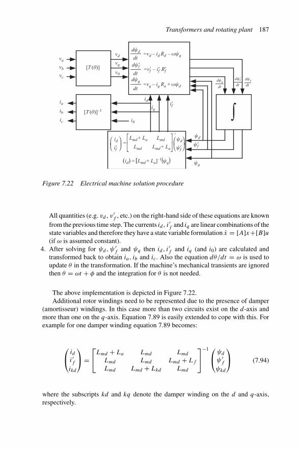
Transformers and rotating plant 187
va
vd
vq
v0
vb
vc
ia
ib
ic i0
idiq
i�f
[T ()]
[T ()]–1
dt
dd
d
=vd – id Rd – �q
dt
dq
q
dt
dqdt
dd
=vq – iq Ra + �d
dt
d�f
�f
dt
d�f
=v�f – i�f R�f
∫ Lmd + La
(id) = [Lmd + La]–1(q)
Lmd Lmd + La
Lmd=
i�f
id�f
d
–1
Figure 7.22 Electrical machine solution procedure
All quantities (e.g. vd, v′f , etc.) on the right-hand side of these equations are known
from the previous time step. The currents id , i′f and iq are linear combinations of thestate variables and therefore they have a state variable formulation x = [A]x+[B]u(if ω is assumed constant).
4. After solving for ψd, ψ ′f and ψq then id , i′f and iq (and i0) are calculated and
transformed back to obtain ia, ib and ic. Also the equation dθ/dt = ω is used toupdate θ in the transformation. If the machine’s mechanical transients are ignoredthen θ = ωt + φ and the integration for θ is not needed.
The above implementation is depicted in Figure 7.22.Additional rotor windings need to be represented due to the presence of damper
(amortisseur) windings. In this case more than two circuits exist on the d-axis andmore than one on the q-axis. Equation 7.89 is easily extended to cope with this. Forexample for one damper winding equation 7.89 becomes:
⎛
⎝idi′fikd
⎞
⎠ =⎡
⎣Lmd + La Lmd Lmd
Lmd Lmd Lmd + Lf
Lmd Lmd + Lkd Lmd
⎤
⎦
−1 ⎛
⎝ψd
ψ ′f
ψkd
⎞
⎠ (7.94)
where the subscripts kd and kq denote the damper winding on the d and q-axis,respectively.
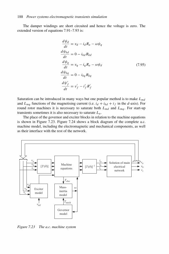
188 Power systems electromagnetic transients simulation
The damper windings are short circuited and hence the voltage is zero. Theextended version of equations 7.91–7.93 is:
dψd
dt= vd − idRa − ωψq
dψkd
dt= 0 − ikdRkd
dψq
dt= vq − iqRa − ωψd
dψkq
dt= 0 − ikqRkq
dψ ′f
dt= v′
f − i′f R′f
(7.95)
Saturation can be introduced in many ways but one popular method is to make Lmd
and Lmq functions of the magnetising current (i.e. id + ikd + if in the d-axis). Forround rotor machines it is necessary to saturate both Lmd and Lmq . For start-uptransients sometimes it is also necessary to saturate La .
The place of the governor and exciter blocks in relation to the machine equationsis shown in Figure 7.23. Figure 7.24 shows a block diagram of the complete a.c.machine model, including the electromagnetic and mechanical components, as wellas their interface with the rest of the network.
Machineequations
Mass-inertiamodel
Solution of main electricalnetwork
Governormodel
Excitermodel
va
va
vc
vc
vb
vbva
vc
vb
ia
ic
ib
vref
Tmech
Telec
[T ()] [T ()]–1
�
Figure 7.23 The a.c. machine system

Transformers and rotating plant 189
EMTDC
Machine equations
dq0Invdq0
Exciter Governor
xNva
vd
vq
v0
idiqi0
iaibic
vb
vc
vref + other �ref + other
vf Tm
if etc.P Q. . .
Figure 7.24 Block diagram synchronous machine model
7.4.4 Types of rotating machine available
Besides the synchronous machine developed by V. Brandwajn, the universal machinemodel was added to EMTP by H.K. Lauw and W.S. Meyer to enable various types ofmachines to be studied using the same model [21], [22]. Under the universal machinemodel the EMTP package includes the following different types of rotating machines:
1. synchronous machine with a three-phase armature2. synchronous machine with a two-phase armature3. induction machine with a three-phase armature4. induction machine with a three-phase armature and three-phase rotor5. induction machine with a two-phase armature6. single-phase induction or synchronous machine with one-phase excitation7. single-phase induction or synchronous machine with two-phase excitation8. d.c. machine separately excited9. d.c. machine with series compound field
10. d.c. machine series excited

190 Power systems electromagnetic transients simulation
11. d.c. machine with parallel compound field12. d.c. machine shunt excited
There are two types of windings, i.e. armature and field windings. Which of themrotates and which are stationary is irrelevent as only the relative motion is important.The armature or power windings are on the stator in the synchronous and inductionmachines and on the rotor in the d.c. machines, with the commutator controlling theflow of current through them.
The user must choose the interface method for the universal machine. There areonly minor differences between the electrical models of the synchronous and universalmachines but their mechanical part differs significantly, and a lumped RLC equivalentelectrical network is used to represent the mechanical part.
Like EMTP the EMTDC program also uses general machine theory for the dif-ferent machines, but with separate FORTRAN subroutines for each machine typeto simplify the parameter entry. For example, the salient pole machine has differentparameters on both axes but only the d-axis mutual saturation is significant; on theother hand the induction machine has the same equivalent circuit in both axes andexperiences saturation of both mutual and leakage reactances. The state variable for-mulation and interfacing detailed in this chapter are the same for all the machines.The machine subroutines can use a different time step and integration procedurefrom the main program. Four machine models are available in EMTDC; the originalsalient pole synchronous machine (MAC100 Model), a new round rotor synchronousmachine model (SNC375), the squirrel cage induction machine (SQC100) and thewound rotor induction motor.
The MAC100 model has been superseded by SNC375, which can model bothsalient and round rotor machines due to the extra damper winding on the q-axis.The squirrel cage induction machine is modelled as a double cage and the motorconvention is used; that is terminal power and shaft torque are positive when poweris going into the machine and the shaft is driving a load.
7.5 Summary
The basic theory of the single-phase transformer has been described, includingthe derivation of parameters, the modelling of magnetisation non-linearities andits numerical implementation in a form acceptable for electromagnetic transientsprograms.
The need for advanced models has been justified, and a detailed description madeof UMEC (the Unified Magnetic Equivalent Circuit), a general transformer modeldeveloped for the accurate representation of multiphase, multiwinding arrangements.UMEC is a standard transformer model in the latest version of PSCAD/EMTDC.
Rotating machine modelling based on Park’s transformation is reasonably stan-dard, the different implementations relating to the way of interfacing the machine tothe system. A state variable formulation of the equations is used but the solution, inline with EMTP philosophy, is carried out by numerical integrator substitution.
Transformers and rotating plant 191
The great variety of rotating machines in existence precludes the use of a commonmodel and so the electromagnetic transient programs include models for the maintypes in current use, most of these based on general machine theory.
7.6 References
1 BRANDWAJN, V., DOMMEL, H. W. and DOMMEL, I. I.: ‘Matrix representa-tion of three-phase n-winding transformers for steady-state and transient studies’,IEEE Transactions on Power Apparatus and Systems, 1982, 101 (6), pp. 1369–78
2 CHEN, M. S. and DILLON, W. E.: ‘Power systems modelling’, Proceedings ofIEEE, 1974, 162 (7), pp. 901–15
3 ARTURI, C. M.: ‘Transient simulation and analysis of a three-phase five-limbstep-up transformer following out-of-phase synchronisation’, IEEE Transactionson Power Delivery, 1991, 6 (1), pp. 196–207
4 DOMMELEN, D. V.: ‘Alternative transients program rule book’, technical report,Leuven EMTP Center, 1987
5 HATZIARGYRIOU, N. D., PROUSALIDIS, J. M. and PAPADIAS, B. C.:‘Generalised transformer model based on analysis of its magnetic circuit’, IEEProceedings Part C, 1993, 140 (4), pp. 269–78
6 CHEN, X. S. and NEUDORFER, P.: ‘The development of a three-phase multi-legged transformer model for use with EMTP’, technical report, Dept. of EnergyContract DE-AC79-92BP26702, USA, 1993
7 LEON, F. D. and SEMLYEN, A.: ‘Complete transformer model for elec-tromagnetic transients’, IEEE Transactions on Power Delivery, 1994, 9 (1),pp. 231–9
8 ENRIGHT, W. G.: ‘Transformer models for electromagnetic transient studieswith particular reference to HVdc transmission’ (Ph.D. thesis, University ofCanterbury, New Zealand, Private Bag 4800, Christchurch, New Zealand, 1996)
9 ENRIGHT, W. G., WATSON, N. R. and ARRILLAGA, J.: ‘Improved simula-tion of HVdc converter transformers in electromagnetic transients programs’,Proceedings of IEE, Part-C, 1997, 144 (2), pp. 100–6
10 BAYLESS, R. S., SELMAN, J. D., TRUAX, D. E. and REID, W. E.: ‘Capacitorswitching and transformer transients’, IEEE Transactions on Power Delivery,1988, 3 (1), pp. 349–57
11 MOMBELLO, E. E. and MOLLER, K.: ‘New power transformer model forthe calculation of electromagnetic resonant transient phenomena includingfrequency-dependent losses’, IEEE Transactions on Power Delivery, 2000, 15(1), pp. 167–74
12 VAN CRAENENBROECK, T., De CEUSTER, J., MARLY, J. P., De HERDT, H.,BROUWERS, B. and VAN DOMMELEN, D.: ‘Experimental and numericalanalysis of fast transient phenomena in distribution transformers’, Proceedingsof Power Engineering Society Winter Meeting, 2000, 3, pp. 2193–8
13 De HERDT, H., DECLERCQ, J., SEIS, T., VAN CRAENENBROECK, T.and VAN DOMMELEN, D.: ‘Fast transients and their effect on transformer
192 Power systems electromagnetic transients simulation
insulation: simulation and measurements’, Electricity Distribution, 2001. Part 1:Contributions. CIRED. 16th International Conference and Exhibition (IEE Conf.Publ No. 482), 2001, Vol. 1, No. 1.6
14 DE LEON, F. and SEMLYEN, A.: ‘Reduced order model for transformertransients’, IEEE Transactions on Power Delivery, 1992, 7 (1), pp. 361–9
15 VAKILIAN, M. and DEGENEFF, R. C.: ‘A method for modeling nonlinear corecharacteristics of transformers during transients’, IEEE Transactions on PowerDelivery, 1994, 9 (4), pp. 1916–25
16 TARASIEWICZ, E. J., MORCHED, A. S., NARANG, A. and DICK, E. P.:‘Frequency dependent eddy current models for nonlinear iron cores’, IEEETransactions on Power Systems, 1993, 8 (2), pp. 588–96
17 SEMLYEN, A. and DE LEON, F.: ‘Eddy current add-on for frequency dependentrepresentation of winding losses in transformer models used in computing elec-tromagnetic transients’, Proceedings of IEE on Generation, Transmission andDistribution (Part C), 1994, 141 (3), pp. 209–14
18 KIMBARK, E. W.: Power system stability; synchronous machines (DoverPublications, New York, 1965)
19 WOODFORD, D. A., GOLE, A. M. and MENZIES, R. W.: ‘Digital simulationof DC links and AC machines’, IEEE Transactions on Power Apparatus andSystems, 1983, 102 (6), pp. 1616–23
20 ADKINS, B. and HARLEY, R. G.: ‘General theory of AC machines’ (Chapman& Hall, London, 1975)
21 LAUW, H. K. and MEYER W. S.: ‘Universal machine modelling for the represen-tation of rotating electric machinery in an electromagnetic transients program’,IEEE Transactions on Power Apparatus and Systems, 1982, 101 (6), pp. 1342–51
22 LAUW, H. K.: ‘Interfacing for universal multi-machine system modelling in anelectromagnetic transients program’, IEEE Transactions on Power Apparatus andSystems, 1985, 104 (9), pp. 2367–73
Chapter 8
Control and protection
8.1 Introduction
As well as accurate modelling of the power components, effective transient simulationrequires detailed representation of their control and protection processes.
A variety of network signals need to be generated as inputs to the control system,such as active and reactive powers, r.m.s. voltages and currents, phase angles, har-monic frequencies, etc. The output of the control functions are then used to controlvoltage and current sources as well as provide switching signals and firing pulses tothe power electronic devices. These signals can also be used to dynamically controlthe values of resistors, inductors and capacitors.
A concise description of the control functions attached to the state variablesolution has been made in Chapter 3. The purpose of this chapter is to discussthe implementation of control and protection systems in electromagnetic transientprograms.
The control blocks, such as integrators, multipliers, etc. need to be translated intoa discrete form for digital computer simulation. Thus the controller itself must also berepresented by difference equations. Although the control equations could be solvedsimultaneously with the main circuit in one large set of linear equations [1], [2],considering the large size of the main circuit, such an approach would result in lossof symmetry and increased computation. Therefore electromagnetic transient pro-grams solve the control equations separately, even though this introduces time-stepdelays in the algorithm. For analogue controls a combined electrical/control solu-tion is also possible, but laborious, by modelling in detail the analogue components(e.g. op-amps, . . .) as electrical components.
The modelling of protection systems in electromagnetic transients programs liesbehind those of other system components. At this stage only a limited number ofrelay types have been modelled and the reliability and accuracy of these models isstill being assessed. Therefore this chapter only provides general guidelines on theireventual implementation.
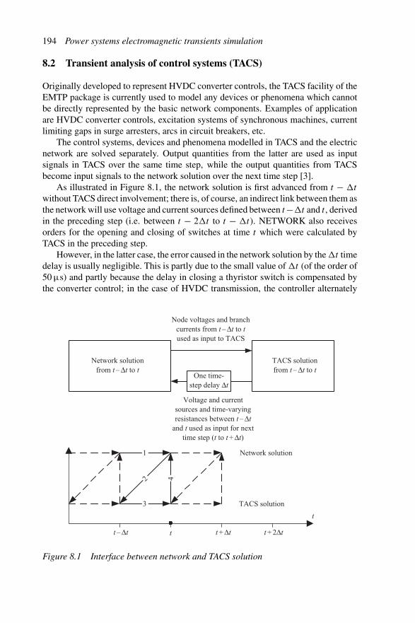
194 Power systems electromagnetic transients simulation
8.2 Transient analysis of control systems (TACS)
Originally developed to represent HVDC converter controls, the TACS facility of theEMTP package is currently used to model any devices or phenomena which cannotbe directly represented by the basic network components. Examples of applicationare HVDC converter controls, excitation systems of synchronous machines, currentlimiting gaps in surge arresters, arcs in circuit breakers, etc.
The control systems, devices and phenomena modelled in TACS and the electricnetwork are solved separately. Output quantities from the latter are used as inputsignals in TACS over the same time step, while the output quantities from TACSbecome input signals to the network solution over the next time step [3].
As illustrated in Figure 8.1, the network solution is first advanced from t − �t
without TACS direct involvement; there is, of course, an indirect link between them asthe network will use voltage and current sources defined between t−�t and t , derivedin the preceding step (i.e. between t − 2�t to t − �t). NETWORK also receivesorders for the opening and closing of switches at time t which were calculated byTACS in the preceding step.
However, in the latter case, the error caused in the network solution by the �t timedelay is usually negligible. This is partly due to the small value of �t (of the order of50 μs) and partly because the delay in closing a thyristor switch is compensated bythe converter control; in the case of HVDC transmission, the controller alternately
Network solution from t – Δt to t
One time- step delay Δt
t
1
4
3
2
Node voltages and branch currents from t – Δt to tused as input to TACS
Voltage and current sources and time-varying resistances between t – Δt
and t used as input for next time step (t to t + Δt)
Network solution
TACS solution
TACS solution from t – Δt to t
t t + Δt t + 2Δtt – Δt
Figure 8.1 Interface between network and TACS solution

Control and protection 195
advances and retards the firing of thyristor switches to keep the power constant duringsteady-state operation.
When a NETWORK solution has been completed, the specified voltage and cur-rent signals are used to derive the TACS solution from t − �t to t ; in this part of theinterface the only time delays are those due to the way in which the control blocksare solved. Any delays can manifest themselves in a steady-state firing error as wellas causing numerical instabilities, particularly if non-linear devices are present.
Besides modelling transfer functions, adders and limiters, TACS allows compo-nents to be modelled using FORTRAN-like functions and expressions. The user canalso supply FORTRAN code as a TACS element [3].
Two approaches can be used to alleviate the effects of time-step delays. Oneinvolves a phase advance technique, using extrapolation to estimate the output of thecontrol solution for the network solution; this method performs poorly during abruptchanges (such as fault inception). The second method reduces the number of internalvariables in the control equations and uses a simultaneous solution of the networkand reduced control equations [1].
MODELS [4] is a general-purpose description language supported by an extensiveset of simulation tools for the representation and study of time-dependent systems.It was first developed in 1985 by Dube and was interfaced to BPA’s EMTP in 1989.MODELS provides an alternative approach to the representation and simulation ofnew components and of control systems in EMTP. However TACS continues to beused for representing simple control systems which can be described using the existingTACS building blocks.
8.3 Control modelling in PSCAD/EMTDC
To help the user to build a complex control system, PSCAD/EMTDC contains aControl Block Library (the Continuous System Model Functions CSMF shown inFigure 8.2). The voltages and currents, used as input to the control blocks, are inte-grated locally (i.e. within each block) to provide flexibility. As explained previouslythis causes a time-step delay in the feedback paths [5]. The delay can be removedby modelling the complete transfer function encompassing the feedback paths, ratherthan using the multiple block representation, however this lacks flexibility.
The trapezoidal discretisation of the control blocks is discussed in Chapter 2.PSCAD simulation is further enhanced by using the exponential form of the
difference equations, as described in Chapter 5, to simulate the various control blocks.With the use of digital controls the time-step delay in the control interface is
becoming less of an issue. Unlike analogue controls, which give an instantaneousresponse, digital controllers sample and hold the continuous voltages and currents,which is effectively what the simulation performs. Modern digital controls havemultiple-time-steps and incorporate event-driven controls, all of which can be mod-elled. EMTDC version 3 has an algorithm which controls the position of time-delayin feedback paths. Rather than using the control library to build a representation ofthe control system, some manufacturers use a direct translation of real control code,

196 Power systems electromagnetic transients simulation
CS
MF
- C
onti
nuou
s S
yste
m M
odel
Fun
ctio
ns
Dig
ital
and
Ana
logu
e C
ontr
ol B
lock
s
*10
.0
GsT
1 +
sT
sT
G1
+ s
T1
1 +
sT
2
G1
+sT
e–sTX
2X
|X|
arc
sin
cos
tan
sin
arc
cos
arc
tan
d/dt
Edg
eD
etec
tor
10x
ex
G1
+ 2
zW
o+
s2s
Wo2
1F
On
OffT
imer
A B
Com
par-
ator
IP
Cle
ar
1 sT
Pha
se
Fre
qM
agS
in
Pha
se
Fre
qM
agC
os
N
D
N/D
D+
F– *
D+
F+
Min
D
E
Max
D
E
N(s
)
D(s
)O
rder
= 1
Low
pas
s bu
tter
wor
thor
der
=3
data
file
dela
y
T
Mon
osta
ble
T
Zer
ode
tect
or
Del
ay
log
X
lnX
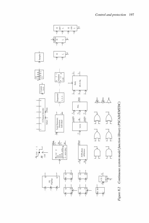
Control and protection 197
Cou
nter
1 to
6J K
Q Q�
J/K
Fli
pflo
p
A B Ctr
lCtr
l=
1
12
34
56
Sel
ect
Dat
a
6 C
hann
el d
ecod
er
Mag
Ph
dc(7)
(7)
F F
T
F =
60.
0 [H
z]
Sam
pler
AP
hase
BX
OR
pha
se
diff
eren
ce
cos(
th)
Vc
th
sin(
th)
VC
O
Va
Vb
Vc
PL
Lth
eta
F
Tot
al H
arm
onic
D
isto
rtio
nIn
divi
dual
7
7
LH
2
H L ON
OF
F
LH
2
Dbl
ck
LH
2D
Q QC
JQ Q
KC
SQ Q
RC
TQ Q
C
SI
SO
C
i ai d
i bi q
i c
thet
a
abc
to d
q
Seq
uent
ial
Ran
dom
30
1
7.7
4 1.01
8
Y
MU
X
I
S4 X
1
1, 2
, 3 .
. .
Fig
ure
8.2
Con
tinu
ous
syst
emm
odel
func
tion
libr
ary
(PSC
AD
/EM
TD
C)

198 Power systems electromagnetic transients simulation
u y+
–
e
G
1
Gs�
Figure 8.3 First-order lag
written in FORTRAN, C, C++, MATLAB or BASIC, and link this with EMTDC.Interpolation of controls is also an important issue for accurate results [6].
8.3.1 Example
The first-order lag control system, depicted in Figure 8.3, is used to demonstrate theuse of the z-domain for the prediction of instabilities.
The corresponding transfer function is:
y
u= 1
1 + fg= G
1 + sτ(8.1)
wheref = feedback path = 1/G
g = forward path = G/(sτ)
τ = time lag.
The equations for the two blocks are:
e = u − 1
Gy (8.2)
y = Ge
sτ(8.3)
Substitution of the trapezoidal rule to form difference equations gives:
ek = uk − 1
Gyk (8.4)
yk = �t(ek + ek−1)G
2τ(8.5)
The difference in data paths becomes apparent. If solved as two separate differenceequations, then ek must be calculated from y at the previous time step as yk is notavailable and this introduces one time-step delay in the y data path. Swapping theorder of equations will result in the same problem for the e data path. Substituting oneequation into the other and rearranging, results in a difference equation with no delay
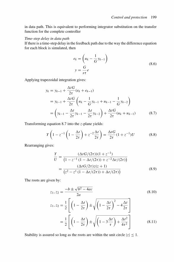
Control and protection 199
in data path. This is equivalent to performing integrator substitution on the transferfunction for the complete controller
Time-step delay in data pathIf there is a time-step delay in the feedback path due to the way the difference equationfor each block is simulated, then
ek =(
uk − 1
Gyk−1
)
y = G
sτe
(8.6)
Applying trapezoidal integration gives:
yk = yk−1 + �tG
2τ(ek + ek−1)
= yk−1 + �tG
2τ
(uk − 1
Gyk−1 + uk−1 − 1
Gyk−2
)
=(
yk−1 − �t
2τyk−1 − �t
2τyk−2
)+ �tG
2τ(uk + uk−1) (8.7)
Transforming equation 8.7 into the z-plane yields:
Y
(1 − z−1
(1 − �t
2τ
)+ z−2 �t
2τ
)= �tG
2τ(1 + z−1)U (8.8)
Rearranging gives:
Y
U= (�tG/(2τ))(1 + z−1)
(1 − z−1 (1 − �t/(2τ)) + z−2�t/(2τ)
)
= (�tG/2τ)z(z + 1)(z2 − z1 (1 − �t/(2τ)) + �t/(2τ)
) (8.9)
The roots are given by:
z1, z2 = −b ± √b2 − 4ac
2a(8.10)
z1, z2 = 1
2
⎡
⎣(
1 − �t
2τ
)±
√(1 − �t
2τ
)2
− 4�t
2τ
⎤
⎦
= 1
2
⎡
⎣(
1 − �t
2τ
)±
√(1 − 3
�t
τ
)+ �t2
4τ 2
⎤
⎦ (8.11)
Stability is assured so long as the roots are within the unit circle |z| ≤ 1.
200 Power systems electromagnetic transients simulation
No time-step delay in data pathIf there is no delay in the feedback path implementation then ek = (uk − (1/G)yk)
Applying trapezoidal integration gives:
yk = yk−1 + �tG
2τ(ek + ek−1)
= yk−1 + �tG
2τ
(uk − 1
Gyk + uk−1 − 1
Gyk−1
)
=(
yk−1 − �t
2τyk − �t
2τyk−1
)+ �tG
2τ(uk + uk−1) (8.12)
Transforming equation 8.12 into the z-plane yields:
Y
((1 + �t
2τ
)+ z−1
(�t
2τ− 1
))= �tG
2τ(1 + z−1)U (8.13)
Rearranging gives:
Y
U= (�tG/(2τ))(1 + z−1)
(1 + �t/(2τ)) + z−1(�t/(2τ) − 1)
= (�tG/(2τ))(z + 1)
z(1 + �t/(2τ)) + (�t/(2τ) − 1)(8.14)
The pole (root of characteristic equation) is:
z = (1 − �t/(2τ))
(1 + �t/(2τ))(8.15)
Note that |zpole| ≤ 1 for all �t/2τ > 0, therefore this method is always stable.However this does not mean that numerical oscillations will not occur due to errorsin the trapezoidal integration.
Root-matching techniqueApplying the root-matching technique to this control system (represented mathemat-ically by equation 8.1) gives the difference equation:
Y (z)
U(z)= G(1 − e−�t/τ )
(1 − z−1e−�t/τ )(8.16)
hence multiplying both side of equation 8.16 by U(z)(1 − z−1e−�t/τ )
Y (z) = e−�t/τ z−1Y (z) + G(1 − e−�t/τ )U(z) (8.17)
Transforming to the time domain yields the difference equation:
yk = e−�t/τ yk−1 + G(1 − e−�t/τ
)uk (8.18)

Control and protection 201
The pole in the z-plane is:
zpole = e−�t/τ (8.19)
Note that |zpole| ≤ 1 for all e−�t/τ ≤ 1 hence for all �t/τ ≥ 0.
Numerical illustrationThe first-order lag system of Figure 8.3 is analysed using the three difference equationsdeveloped previously, i.e. the trapezoidal rule with no feedback (data path) delay, thetrapezoidal rule with data path delay and the exponential form using the root-matchingtechnique. The step response is considered using three different time-steps, �t =τ/10, τ, 10τ (τ = 50 μs) and the corresponding results are shown in Figures 8.4–8.6.
When �t/τ = 1/10 the poles for trapezoidal integration with delay in the datapath are obtained by solving equation 8.11; these are:
z1, z2 = 19
20±
√√√√
((19
20
)2
− 4
20
)
= 0.0559 and 0.8941
Since two real roots exist (z1 = 0.0559 and z2 = 0.894) and both are smaller thanone, the resulting difference equation is stable. This can clearly be seen in Figure 8.4,which also shows that the exponential form (pole = 0.9048) and the trapezoidalrule (pole = 0.9048) with no data path delay are indistinguishable, while the errorintroduced by the trapezoidal rule with data path delay is noticeable.
0
0.2
0.4
0.6
0.8
1
1.2
y
Time (s)
Trapezoidal Trapezoidal (time-step delay) Exponential form
0.0009 0.001 0.0011 0.0012 0.0013
Figure 8.4 Simulation results for a time step of 5 μs
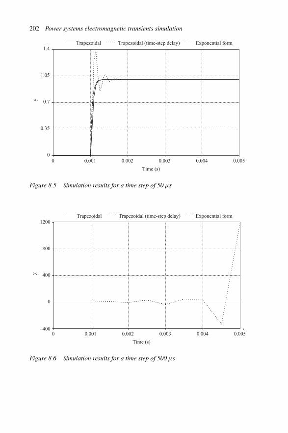
202 Power systems electromagnetic transients simulationy
Time (s)
Trapezoidal Trapezoidal (time-step delay) Exponential form
0 0.001 0.002 0.003 0.004 0.0050
0.35
0.7
1.05
1.4
Figure 8.5 Simulation results for a time step of 50 μs
y
Time (s)
Trapezoidal Trapezoidal (time-step delay) Exponential form
0
400
800
1200
–4000 0.001 0.002 0.003 0.004 0.005
Figure 8.6 Simulation results for a time step of 500 μs

Control and protection 203
The poles when �t/τ = 1 are given by:
z1, z2 = 1
2
⎛
⎝1
2±
√√√√((
1
2
)2
− 41
2
)⎞
⎠ = 0.25 ± j0.6614
Hence a pair of complex conjugate roots result (z1, z2 = 0.25 ± j0.6614). Theylie inside the unit circle (|z1| = |z2| = 0.7071 < 1) which indicates stability.Figure 8.5 shows that, although considerable overshoot has been introduced by thetime-step delay in the data path, this error dies down in approximately 20 time stepsand the difference equations are stable. A slight difference can be seen between thetrapezoidal integrator with no data delay (pole = 0.3333) and the exponential form(pole = 0.3679).
Finally when �t/τ = 10 the poles for the trapezoidal rule with time delay in thefeedback path are:
z1, z2 = −4
2±
√((−4)2 − 4 × 5)
2= −2.0 ± j1.0
hence two complex poles exist, however they lie outside the unit circle in the z-planeand therefore the system of difference equations is unstable. This is shown in thesimulation results in Figure 8.6.
The poles for the trapezoidal method with no time delay and exponential form are−0.6667 and 4.5400e−005 respectively. As predicted by equation 8.15, the differenceequation with no data path delay is always stable but close examination of an expandedview (displayed in Figure 8.6) shows a numerical oscillation in this case. Moreover,this numerical oscillation will increase with the step length. Figure 8.6 also showsthe theoretical curve and exponential form of the difference equation. The latter givesthe exact answer at every point it is evaluated. The exponential form has been derivedfor the overall transfer function (i.e. without time delays in the data paths).
If a modular building block approach is adopted, the exponential form of dif-ference equation can be applied to the various blocks, and the system of differenceequations is solved in the same way as for the trapezoidal integrator. However, errorsdue to data path delays will occur. This detrimental effect results from using a modularapproach to controller representation.
This example has illustrated the use of the z-domain in analysing the differenceequations and data path delays and shown that with z-domain analysis instabilitiescan be accurately predicted. Modelling the complete controller transfer function ispreferable to a modular building block approach, as it avoids the data path delaysand inherent error associated with it, which can lead to instabilities. However theerror introduced by the trapezoidal integrator still exists and the best solution is touse instead the exponential form of difference equation derived from root-matchingtechniques.
As well as control blocks, switches and latches, the PSCAD/EMTDC CSMFlibrary contains an on-line Fourier component that is used to derive the frequencycomponents of signals. It uses a Discrete Fourier Transform rather than an FFT. This
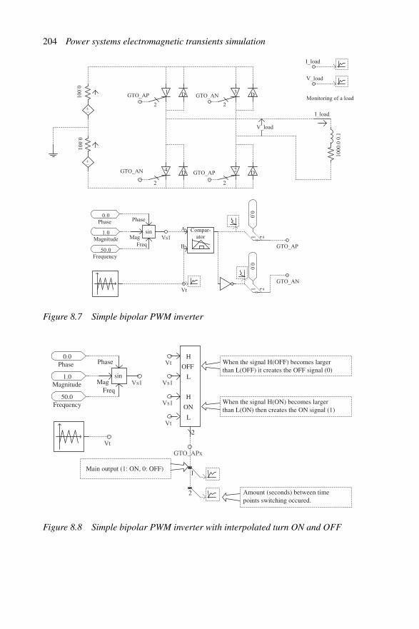
204 Power systems electromagnetic transients simulation
1.0Magnitude
Phase
FreqMag
sin
0.0Phase
50.0Frequency
0.001 1
2
D
0.001
D
4
2
D 2
2
D
1000
.0 0
.1
V_load
I_load
I_load
V_load
GTO_AP
GTO_AN
1 2
0.0
1 2
0.0
Vs1
Vt
Monitoring of a loadGTO_AP
GTO_AP
GTO_AN
GTO_AN
3
2
A
B
Compar-ator
+–
+–
Figure 8.7 Simple bipolar PWM inverter
1.0Magnitude
Phase
FreqMag
sin
0.0Phase
50.0Frequency Vs1
Vt
Vt
Vs1
GTO_APx
1
2
Vt
Vs1
When the signal H(OFF) becomes larger than L(OFF) it creates the OFF signal (0)
L
H
2
H
L
ON
OFF
When the signal H(ON) becomes larger than L(ON) then creates the ON signal (1)
Amount (seconds) between time points switching occured.
Main output (1: ON, 0: OFF)
Figure 8.8 Simple bipolar PWM inverter with interpolated turn ON and OFF
Control and protection 205
enables a recursive formulation to be used, which is very efficient computationally,especially when a small number of frequency components are required (the maximumlimit is 31 for the on-line Fourier component).
Figure 8.7 displays a simple bipolar inverter, where the valve is turned on atthe first time point after the crossover of the triangular and control signals. To takeadvantage of interpolated switching the interpolated firing pulses block is used asshown in Figure 8.8.
8.4 Modelling of protective systems
A protective system consists of three main components, i.e. transducers, relays andcircuit breakers, all of which require adequate representation in electromagnetictransients programs.
The modelling of the relays is at present the least advanced, due to insufficientdesign information from manufacturers. This is particularly a problem in the caseof modern microprocessor-based relays, because a full description of the softwareinvolved would give the design secrets away! Manufacturers’ manuals contain mostlyrelay behaviour in the form of operating characteristics in terms of phasor parameters.Such information, however, is not sufficient to model the relay behaviour undertransient conditions. PSCAD/EMTDC does allow manufacturers to provide binarylibrary files of their custom models which can be used as a ‘black-box’, thus keepingtheir design secret.
Even if all the design details were available, it would be an extremely complexexercise to model all the electronic, electromechanical and software components ofthe relay. A more practical approach is to develop models that match the behaviourof the actual relays under specified operating conditions.
A practical way of developing suitable models is by means of comprehensivevalidation, via physical testing of the actual relays and their intended models. TheReal-Time Playback (RTP) system or Real-Time Digital Simulator (RTDS), describedin Chapter 13, provide the ideal tools for that purpose. The RTDS performs electro-magnetic transient simulation to provide the fault current and voltage waveforms indigital form. These are converted to analogue signals by means of A/D convertersand then amplified to the appropriate levels required by the relay.
Recognising the importance of relay modelling, a Working Group of the IEEEPower System Relaying Committee has recently published a paper reviewing thepresent state of the art in relay modelling and recommending guidelines for furtherwork [7].
8.4.1 Transducers
The performance of high-speed protection is closely related to the response of theinstrumentation transformers to the transient generated by the power system. There-fore, to be effective, electromagnetic transient programs require adequate modellingof the current transformers, magnetic voltage transformers and capacitor voltagetransformers. A Working Group (WG C-5) of the Systems Protection Subcommittee
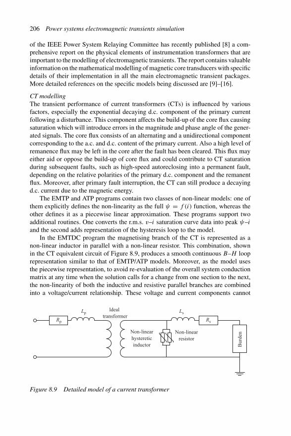
206 Power systems electromagnetic transients simulation
of the IEEE Power System Relaying Committee has recently published [8] a com-prehensive report on the physical elements of instrumentation transformers that areimportant to the modelling of electromagnetic transients. The report contains valuableinformation on the mathematical modelling of magnetic core transducers with specificdetails of their implementation in all the main electromagnetic transient packages.More detailed references on the specific models being discussed are [9]–[16].
CT modellingThe transient performance of current transformers (CTs) is influenced by variousfactors, especially the exponential decaying d.c. component of the primary currentfollowing a disturbance. This component affects the build-up of the core flux causingsaturation which will introduce errors in the magnitude and phase angle of the gener-ated signals. The core flux consists of an alternating and a unidirectional componentcorresponding to the a.c. and d.c. content of the primary current. Also a high level ofremanence flux may be left in the core after the fault has been cleared. This flux mayeither aid or oppose the build-up of core flux and could contribute to CT saturationduring subsequent faults, such as high-speed autoreclosing into a permanent fault,depending on the relative polarities of the primary d.c. component and the remanentflux. Moreover, after primary fault interruption, the CT can still produce a decayingd.c. current due to the magnetic energy.
The EMTP and ATP programs contain two classes of non-linear models: one ofthem explicitly defines the non-linearity as the full ψ = f (i) function, whereas theother defines it as a piecewise linear approximation. These programs support twoadditional routines. One converts the r.m.s. v–i saturation curve data into peak ψ–i
and the second adds representation of the hysteresis loop to the model.In the EMTDC program the magnetising branch of the CT is represented as a
non-linear inductor in parallel with a non-linear resistor. This combination, shownin the CT equivalent circuit of Figure 8.9, produces a smooth continuous B–H looprepresentation similar to that of EMTP/ATP models. Moreover, as the model usesthe piecewise representation, to avoid re-evaluation of the overall system conductionmatrix at any time when the solution calls for a change from one section to the next,the non-linearity of both the inductive and resistive parallel branches are combinedinto a voltage/current relationship. These voltage and current components cannot
Lp Ls
Rp Rs
ldealtransformer
Non-linearhystereticinductor
Non-linearresistor
Bur
den
Figure 8.9 Detailed model of a current transformer

Control and protection 207
100
80
60
40
20
0
–20
–40
–60
–80
Cur
rent
(am
ps)
Time (ms)
25 50 75 100
80
60
40
20
0
–20
–40
–60
–80
Cur
rent
(am
ps)
Time (ms)
25 50 75 100
(a)
(b)
Figure 8.10 Comparison of EMTP simulation (solid line) and laboratory data (dot-ted line) with high secondary burden. (a) without remanence in the CT;(b) with remanence in the CT.
be calculated independently of each other, and an exact solution would require aniterative solution. However, various techniques have been suggested to reduce thesimulation time in this respect [9].
Other important CT alternatives described by the Working Group document arethe Seetee [15] and the Jiles–Atherton [13] models. All these models have been testedin the laboratory and shown to produce reasonable and practically identical results.An example of the comparison between the EMTP simulation and laboratory data isshown in Figure 8.10. These results must be interpreted with caution when trying toduplicate them, because there is no information on the level of CT remanence, if any,present in the laboratory tests.
CVT modellingIn the CVT the voltage transformation is achieved by a combination of a capacitivedivider, which achieves the main step-down in voltage, and a small wound voltage
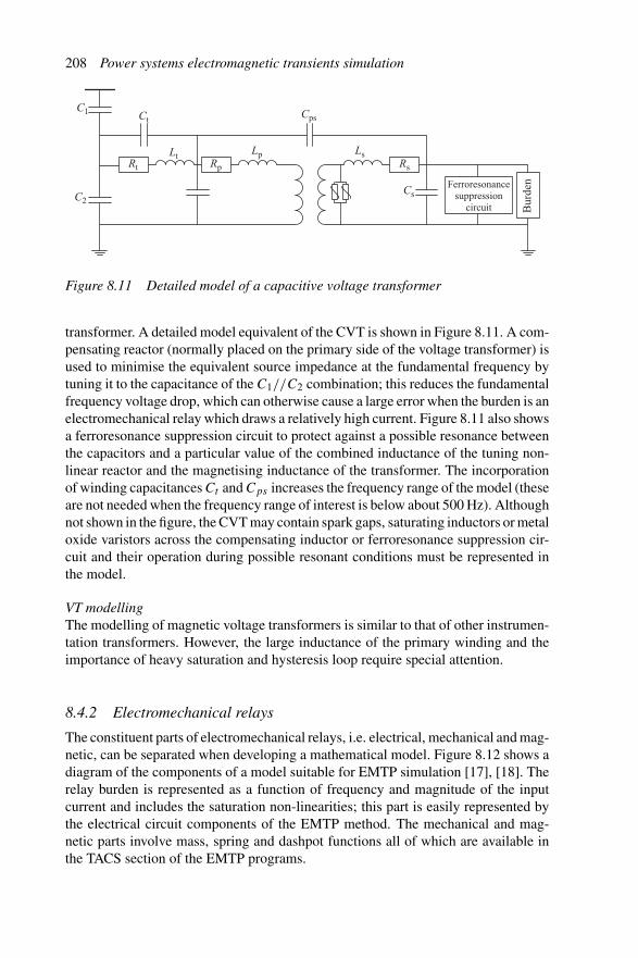
208 Power systems electromagnetic transients simulation
C2
C1 Ct Cps
Rt Rp Rs
Lp Ls
Cs
Lt
Bur
denFerroresonance
suppressioncircuit
Figure 8.11 Detailed model of a capacitive voltage transformer
transformer. A detailed model equivalent of the CVT is shown in Figure 8.11. A com-pensating reactor (normally placed on the primary side of the voltage transformer) isused to minimise the equivalent source impedance at the fundamental frequency bytuning it to the capacitance of the C1//C2 combination; this reduces the fundamentalfrequency voltage drop, which can otherwise cause a large error when the burden is anelectromechanical relay which draws a relatively high current. Figure 8.11 also showsa ferroresonance suppression circuit to protect against a possible resonance betweenthe capacitors and a particular value of the combined inductance of the tuning non-linear reactor and the magnetising inductance of the transformer. The incorporationof winding capacitances Ct and Cps increases the frequency range of the model (theseare not needed when the frequency range of interest is below about 500 Hz). Althoughnot shown in the figure, the CVT may contain spark gaps, saturating inductors or metaloxide varistors across the compensating inductor or ferroresonance suppression cir-cuit and their operation during possible resonant conditions must be represented inthe model.
VT modellingThe modelling of magnetic voltage transformers is similar to that of other instrumen-tation transformers. However, the large inductance of the primary winding and theimportance of heavy saturation and hysteresis loop require special attention.
8.4.2 Electromechanical relays
The constituent parts of electromechanical relays, i.e. electrical, mechanical and mag-netic, can be separated when developing a mathematical model. Figure 8.12 shows adiagram of the components of a model suitable for EMTP simulation [17], [18]. Therelay burden is represented as a function of frequency and magnitude of the inputcurrent and includes the saturation non-linearities; this part is easily represented bythe electrical circuit components of the EMTP method. The mechanical and mag-netic parts involve mass, spring and dashpot functions all of which are available inthe TACS section of the EMTP programs.
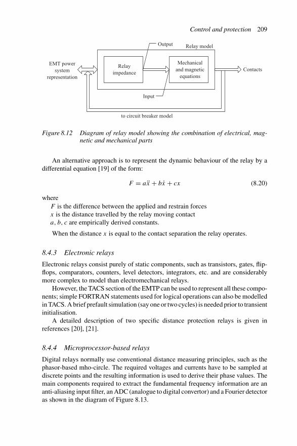
Control and protection 209
Relayimpedance
Mechanicaland magnetic
equations
Output
Input
ContactsEMT power
systemrepresentation
Relay model
to circuit breaker model
Figure 8.12 Diagram of relay model showing the combination of electrical, mag-netic and mechanical parts
An alternative approach is to represent the dynamic behaviour of the relay by adifferential equation [19] of the form:
F = ax + bx + cx (8.20)
whereF is the difference between the applied and restrain forcesx is the distance travelled by the relay moving contacta, b, c are empirically derived constants.
When the distance x is equal to the contact separation the relay operates.
8.4.3 Electronic relays
Electronic relays consist purely of static components, such as transistors, gates, flip-flops, comparators, counters, level detectors, integrators, etc. and are considerablymore complex to model than electromechanical relays.
However, the TACS section of the EMTP can be used to represent all these compo-nents; simple FORTRAN statements used for logical operations can also be modelledin TACS. A brief prefault simulation (say one or two cycles) is needed prior to transientinitialisation.
A detailed description of two specific distance protection relays is given inreferences [20], [21].
8.4.4 Microprocessor-based relays
Digital relays normally use conventional distance measuring principles, such as thephasor-based mho-circle. The required voltages and currents have to be sampled atdiscrete points and the resulting information is used to derive their phase values. Themain components required to extract the fundamental frequency information are ananti-aliasing input filter, an ADC (analogue to digital convertor) and a Fourier detectoras shown in the diagram of Figure 8.13.
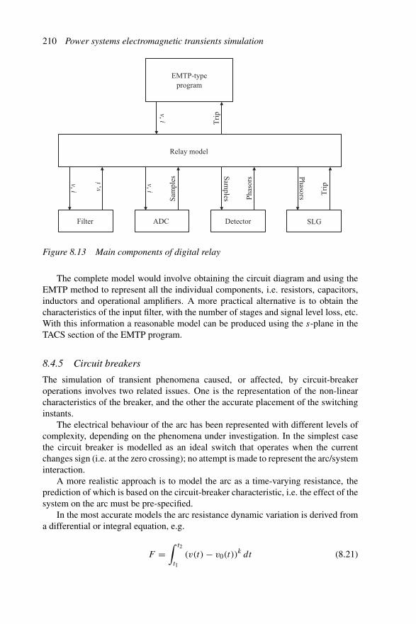
210 Power systems electromagnetic transients simulation
EMTP-typeprogram
Relay model
Filter ADC Detector
v,i
v,i
v,iv,i
Sam
ples
Pha
sors
Tri
p
Tri
p
Phasors
Sam
ples
SLG
Figure 8.13 Main components of digital relay
The complete model would involve obtaining the circuit diagram and using theEMTP method to represent all the individual components, i.e. resistors, capacitors,inductors and operational amplifiers. A more practical alternative is to obtain thecharacteristics of the input filter, with the number of stages and signal level loss, etc.With this information a reasonable model can be produced using the s-plane in theTACS section of the EMTP program.
8.4.5 Circuit breakers
The simulation of transient phenomena caused, or affected, by circuit-breakeroperations involves two related issues. One is the representation of the non-linearcharacteristics of the breaker, and the other the accurate placement of the switchinginstants.
The electrical behaviour of the arc has been represented with different levels ofcomplexity, depending on the phenomena under investigation. In the simplest casethe circuit breaker is modelled as an ideal switch that operates when the currentchanges sign (i.e. at the zero crossing); no attempt is made to represent the arc/systeminteraction.
A more realistic approach is to model the arc as a time-varying resistance, theprediction of which is based on the circuit-breaker characteristic, i.e. the effect of thesystem on the arc must be pre-specified.
In the most accurate models the arc resistance dynamic variation is derived froma differential or integral equation, e.g.
F =∫ t2
t1
(v(t) − v0(t))k dt (8.21)

Control and protection 211
where v0 and k are constants, and t2 is the instant corresponding to voltage breakdown,which occurs when the value of F reaches a user-defined value.
In the BPA version the voltage–time characteristic is simulated by an auxiliaryswitch in which the breakdown is controlled by a firing signal received from the TACSpart of the EMTP.
The above considerations refer to circuit breaking. The modelling requirementsare different for the circuit-making action. In the latter case the main factor affectingthe transient overvoltage peak is the closing instant. Since that instant (which isdifferent in each phase) is not normally controllable, transient programs tend to usestatistical distributions of the switching overvoltages.
Considering the infrequent occurrence of power system faults, the switchings thatfollow protection action add little overhead to the EMTP simulation process.
8.4.6 Surge arresters
Power system protection also includes insulation coordination, mostly carried out bymeans of surge arresters [22].
Most arresters in present use are of the silicon carbide and metal oxide types. Theformer type uses a silicon carbide resistor in series with a spark gap. When the over-voltage exceeds the spark-over level (Figure 8.14) the spark gap connects the arresterto the network; the resistor, which has a non-linear voltage/current characteristic (suchas shown in Figure 8.15) then limits the current through the arrester.
Time00
Incomingwave
Breakdownoccurs
VBreakdown
Vol
tage
Figure 8.14 Voltage–time characteristic of a gap

212 Power systems electromagnetic transients simulation
0 1 2 3 4 5 6 7 8 9 10Current (kA)
Vol
tage
(kV
)Vsparkover = 610 kV
Current (kA) Voltage(kV)
0
100
200
300
400
500
600
700
0.0 00.51.01.52.53.0
10.0
440510540580590660
Figure 8.15 Voltage–time characteristic of silicon carbide arrestor
In the EMTP the silicon carbide arrester is modelled as a non-linear resistance inseries with a gap (of constant spark-over voltage). In practice the spark-over voltageis dependent on the steepness of the income voltage waveshape; this is difficult toimplement, given the irregular shape of the surges.
The non-linear resistance in series with the gap can be solved either bycompensation techniques [22] or via piecewise linear models.
Metal oxide surge arresters contain highly non-linear resistances, with practicallyinfinite slope in the normal voltage region and an almost horizontal slope in the pro-tected region. Such characteristics, shown typically in Figure 8.16, are not amenableto a piecewise linear representation. Therefore in the EMTP programs metal oxidearresters are usually solved using the compensation method.
Interpolation is important in modelling arresters to determine the time point wherethe characteristic of the arrester changes. The energy calculation in the EMTDCprogram is interpolated to ensure a realistic result. Special care is needed in thelow-current region when carrying out trapped charge studies.
Metal oxide arresters are frequency-dependent devices (i.e. the voltage acrossthe arrester is a function of both the rate of rise and the magnitude of the current)and therefore the model must be consistent with the frequency or time-to-crest of thevoltage and current expected from the disturbance. Figure 8.17 shows the frequency-dependent model of the metal oxide arrester proposed by the IEEE [22]. In the absenceof a frequency-dependent model the use of simple non-linear V –I characteristics,derived from test data with appropriate time-to-crest waveforms, is adequate.

Control and protection 213
2000
1000
500
200
100
1 100.01 104
Vol
tage
(kV
)
Current (A)
Figure 8.16 Voltage–time characteristic of metal oxide arrestor
L0
R0R1
L1
A0 A1
C
Figure 8.17 Frequency-dependent model of metal oxide arrestor
8.5 Summary
The control equations are solved separately from the power system equations thoughstill using the EMTP philosophy, thereby maintaining the symmetry of the conduc-tance matrix. The main facilities developed to segment the control, as well as devicesor phenomena which cannot be directly modelled by the basic network components,are TACS and MODELS (in the original EMTP package) and a CMSF library (in thePSCAD/EMTDC package).
The separate solution of control and power system introduces a time-step delay,however with the sample and hold used in digital control this is becoming less of anissue. Modern digital controls, with multiple time steps, are more the norm and canbe adequately represented in EMT programs.
214 Power systems electromagnetic transients simulation
The use of a modular approach to build up a control system, although it givesgreater flexibility, introduces time-step delays in data paths, which can have a detri-mental effect on the simulation results. The use of the z-domain for analysing thedifference equations either generated using NIS, with and without time-step delay, orthe root-matching technique, has been demonstrated.
Interpolation is important for modelling controls as well as for the non-linearsurge arrester, if numerical errors and possible instabilities are to be avoided.
A description of the present state of protective system implementation has beengiven, indicating the difficulty of modelling individual devices in detail. Instead,the emphasis is on the use of real-time digital simulators interfaced with the actualprotection hardware via digital-to-analogue conversion.
8.6 References
1 ARAUJO, A. E. A., DOMMEL, H. W. and MARTI, J. R.: ‘Converter simulationswith the EMTP: simultaneous solution and backtracking technique’, IEEE/NTUAAthens Power Tech Conference Planning, Operation and Control of Today’sElectric Power Systems, September 5–8, 1993, 2, pp. 941–5
2 ARAUJO, A. E. A., DOMMEL, H. W. and MARTI, J. R.: ‘Simultaneous solutionof power and control system equations’, IEEE Transactions on Power Systems,1993, 8 (4), pp. 1483–9
3 LASSETER, R. H. and ZHOU, J.: ‘TACS enhancements for the electromagnetictransient program’, IEEE Transactions on Power Systems, 1994, 9 (2), pp. 736–42
4 DUBE, L. and BONFANTI, I.: ‘MODELS: a new simulation tool in EMTP’,1992, ETEP 2 (1), pp. 45–50
5 WATSON, N. R. and IRWIN, G. D.: ‘Accurate and stable electromagnetic transientsimulation using root-matching techniques’, International Journal of ElectricalPower & Energy Systems, Elsevier Science Ltd, 1999, 21 (3), pp. 225–34
6 GOLE, A. M. and NORDSTROM, J. E.: ‘A fully interpolated controls library forelectromagnetic transients simulation of power electronic systems’, Proceedingsof International Conference on Power system transients (IPST’2001), June 2001,pp. 669–74
7 McLAREN, P. G., MUSTAPHI, K., BENMOUYAL, G. et al.: ‘Software modelsfor relays’, IEEE Transactions on Power Delivery, 2001, 16 (2), pp. 238–45
8 Working Group C5 of the Systems Protection subcommittee of the IEEE PowerSystem Relaying Committee: ‘Mathematical models for current, voltage, andcoupling capacitor voltage transformer’, IEEE Transactions on Power Delivery,2000, 15 (1), pp. 62–72
9 LUCAS, J. R., McLAREN, P. G. and JAYASINGHE, R. P.: ‘Improved simulationmodels for current and voltage transformers in relay studies’, IEEE Trans. onPower Delivery, 1992, 7 (1), p. 152
10 WISEMAN, M. J.: ‘CVT transient behavior during shunt capacitor switching’,Ontario Hydro study no. W401, April 1993
Control and protection 215
11 McLAREN, P. G., LUCAS, J. R. and KEERTHIPALA, W. W. L.: ‘A digitalsimulation model for CCVT in relay studies’, Proceedings International PowerEngineering Conference (IPEC), March 1993
12 KOJOVIC, L. A., KEZUNOVIC, M. and NILSSON, S. L.: ‘Computer simulationof a ferroresonance suppression circuit for digital modeling of coupling capacitorvoltage transformers’, ISMM International Conference, Orlando, Florida, 1992
13 JILES, D. C. and ATHERTON, D. L.: ‘Theory of ferromagnetic hysteresis’,Journal of Magnetism and Magnetic Materials, 1986, 61, pp. 48–60
14 JILES, D. C., THOELKE, J. B. and DEVINE, M. K.: ‘Numerical determinationof hysteresis parameters for modeling of magnetic properties using the theoryof ferromagnetic hysteresis’, IEEE Transactions on Magnetics, 1992, 28 (1),pp. 27–334
15 GARRET, R., KOTHEIMER, W. C. and ZOCHOLL, S. E.: ‘Computer simulationof current transformers and relays’, Proceedings of 41st Annual Conference forProtective Relay Engineers, 1988, Texas A&M University
16 KEZUNOVIC, M., KOJOVIC, L. J., ABUR, A., FROMEN, C. W. andSEVCIK, D. R.: ‘Experimental evaluation of EMTP-based current transformermodels for protective relay transient study’, IEEE Transactions on PowerDelivery, 1994, 9 (1), pp. 405–13
17 GLINKOWSKI, M. T. and ESZTRGALYOS, J.: ‘Transient modeling of electro-mechanical relays. Part 1: armature type relay’, IEEE Transactions on PowerDelivery, 1996, 11 (2), pp. 763–70
18 GLINKOWSKI, M. T. and ESZTRGALYOS, J.: ‘Transient modeling of electro-mechanical relays. Part 2: plunger type 50 relays’, IEEE Transactions on PowerDelivery, 1996, 11 (2), pp. 771–82
19 CHAUDARY, A. K. S, ANICH, J. B. and WISNIEWSKI, A.: ‘Influence of tran-sient response of instrument transformers on protection systems’, Proceedings ofSargent and Lundy, 12th biennial Transmission and Substation Conference, 1992
20 GARRETT, B. W.: ‘Digital simulation of power system protection under transientconditions’ (Ph.D. thesis, University of British Columbia, 1987)
21 CHAUDHARY, A. K. S., TAM, K.-S. and PHADKE, A. G.: ‘Protection systemrepresentation in the electromagnetic transients program’, IEEE Transactions onPower Delivery, 1994, 9 (2), pp. 700–11
22 IEEE Working Group on Surge Arrester Modeling: ‘Modeling of metal oxidesurge arresters’, IEEE Transactions on Power Delivery, 1992, 1 (1), pp. 302–9

Chapter 9
Power electronic systems
9.1 Introduction
The computer implementation of power electronic devices in electromagnetictransient programs has taken much of the development effort in recent years, aimingat preserving the elegance and efficiency of the EMTP algorithm. The main featurethat characterises power electronic devices is the use of frequent periodic switchingof the power components under their control.
The incorporation of power electronics in EMT simulation is discussed in thischapter with reference to the EMTDC version but appropriate references are made,as required, to other EMTP-based algorithms. This is partly due to the fact that theEMTDC program was specifically developed for the simulation of HVDC transmis-sion and partly to the authors’ involvement in the development of some of its recentcomponents. A concise description of the PSCAD/EMTDC program structure is givenin Appendix A.
This chapter also describes the state variable implementation of a.c.–d.c. convert-ers and systems, which offers some advantages over the EMTP solution, as well as ahybrid algorithm involving both the state variable and EMTP methods.
9.2 Valve representation in EMTDC
In a complex power electronic system, such as HVDC transmission, valves con-sist of one or more series strings of thyristors. Each thyristor is equipped with aresistor–capacitor damping or snubber circuit. One or more di/dt limiting inductorsare included in series with the thyristors and their snubber circuits. It is assumedthat for most simulation purposes, one equivalent thyristor, snubber circuit and di/dt
limiting inductor will suffice for a valve model. The di/dt limiting inductor canusually be neglected when attempting transient time domain simulations up to about1.5–2.0 kHz frequency response. In version 3 of the EMTDC program the snubber iskept as a separate branch to allow chatter removal to be effective.

218 Power systems electromagnetic transients simulation
Cd
Valve
k
m
jRv
Rd
Snubbercircuit
equivalent
k
m
ikm(t)
ikm (t – Δt)
Figure 9.1 Equivalencing and reduction of a converter valve
EMTDC V2 utilised the fact that network branches of inductors and capacitorsare represented as resistors with an associated current source, which allowed a valvein a converter bridge to be represented by the Norton equivalent of Figure 9.1.
With the valve blocked (not conducting), the equivalent resistor Rv is just derivedfrom the snubber circuit. With the di/dt limiting inductor ignored, then fromreference [1] this becomes:
Rv = Rd + �t
2Cd
(9.1)
where�t = time-step lengthRd = snubber resistanceCd = snubber capacitance
With the valve de-blocked and conducting in the forward direction, the equivalentresistor Rv is changed to a low value, e.g. Rv = 1 �. The equivalent current sourceIkm(t−�t) shown in Figure 9.1 between nodes k and m is determined by first definingthe ratio Y as:
Y = �t/(2Cd)
Rd + �t/(2Cd)(9.2)
From equations 4.11 and 4.13 of Chapter 4.
ikm(t) = (ek(t) − em(t))
Rd + �t/(2Cd)+ Ikm(t − �t) (9.3)
then
Ikm(t − �t) = −Y
[ikm(t − �t) + 2Cd
(ej (t − �t) − em(t − �t))
�t
](9.4)
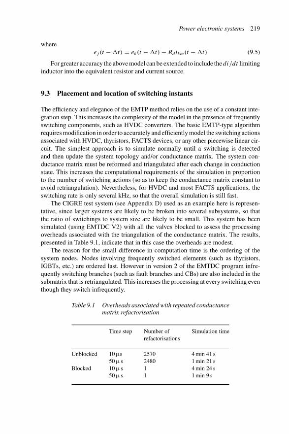
Power electronic systems 219
whereej (t − �t) = ek(t − �t) − Rdikm(t − �t) (9.5)
For greater accuracy the above model can be extended to include the di/dt limitinginductor into the equivalent resistor and current source.
9.3 Placement and location of switching instants
The efficiency and elegance of the EMTP method relies on the use of a constant inte-gration step. This increases the complexity of the model in the presence of frequentlyswitching components, such as HVDC converters. The basic EMTP-type algorithmrequires modification in order to accurately and efficiently model the switching actionsassociated with HVDC, thyristors, FACTS devices, or any other piecewise linear cir-cuit. The simplest approach is to simulate normally until a switching is detectedand then update the system topology and/or conductance matrix. The system con-ductance matrix must be reformed and triangulated after each change in conductionstate. This increases the computational requirements of the simulation in proportionto the number of switching actions (so as to keep the conductance matrix constant toavoid retriangulation). Nevertheless, for HVDC and most FACTS applications, theswitching rate is only several kHz, so that the overall simulation is still fast.
The CIGRE test system (see Appendix D) used as an example here is represen-tative, since larger systems are likely to be broken into several subsystems, so thatthe ratio of switchings to system size are likely to be small. This system has beensimulated (using EMTDC V2) with all the valves blocked to assess the processingoverheads associated with the triangulation of the conductance matrix. The results,presented in Table 9.1, indicate that in this case the overheads are modest.
The reason for the small difference in computation time is the ordering of thesystem nodes. Nodes involving frequently switched elements (such as thyristors,IGBTs, etc.) are ordered last. However in version 2 of the EMTDC program infre-quently switching branches (such as fault branches and CBs) are also included in thesubmatrix that is retriangulated. This increases the processing at every switching eventhough they switch infrequently.
Table 9.1 Overheads associated with repeated conductancematrix refactorisation
Time step Number of Simulation timerefactorisations
Unblocked 10 μs 2570 4 min 41 s50 μ s 2480 1 min 21 s
Blocked 10 μ s 1 4 min 24 s50 μ s 1 1 min 9 s
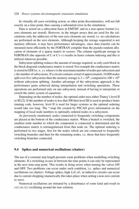
220 Power systems electromagnetic transients simulation
In virtually all cases switching action, or other point discontinuities, will not fallexactly on a time point, thus causing a substantial error in the simulation.
Data is stored on a subsystem basis in EMTDC and in a non-sparse format (i.e.zero elements are stored). However, in the integer arrays that are used for the cal-culations only the addresses of the non-zero elements are stored, i.e. no calculationsare performed on the zero elements. Although keeping the storage sequential is notmemory efficient, it may have performance advantages, since data transfer can bestreamed more efficiently by the FORTRAN compiler than the pseudo-random allo-cation of elements of a sparse matrix in vectors. The column significant storage inFORTRAN (the opposite of C or C++) results in faster column indexing and this isutilized wherever possible.
Subsystem splitting reduces the amount of storage required, as only each block inthe block diagonal conductance matrix is stored. For example the conductance matrixis stored in GDC(n, n, s), where n is the maximum number of nodes per subsystem ands the number of subsystems. If a circuit contains a total of approximately 10,000 nodessplit over five subsystems then the memory storage is 2×10⁶, compared to 100×106
without subsystem splitting. Another advantage of the subsystems approach is theperformance gains achieved during interpolation and switching operations. Theseoperations are performed only on one subsystem, instead of having to interpolate orswitch the entire system of equations.
Depending on the number of nodes, the optimal order uses either Tinney’s level IIor III [2]. If the number of nodes is less that 500 then level III is used to produce fasterrunning code, however, level II is used for larger systems as the optimal orderingwould take too long. The *.map file created by PSCAD gives information on themapping of local node numbers to optimally ordered nodes in a subsystem.
As previously mentioned, nodes connected to frequently switching componentsare placed at the bottom of the conductance matrix. When a branch is switched, thesmallest node number to which the component is connected is determined and theconductance matrix is retriangularised from that node on. The optimal ordering isperformed in two stages, first for the nodes which are not connected to frequentlyswitching branches and then for the remaining nodes, i.e. those that have frequentlyswitching branches connected.
9.4 Spikes and numerical oscillations (chatter)
The use of a constant step length presents some problems when modelling switchingelements. If a switching occurs in between the time points it can only be representedat the next time-step point. This results in firing errors when turning the valves ONand OFF. Two problems can occur under such condition, i.e. spikes and numericaloscillations (or chatter). Voltage spikes, high Ldi/dt , in inductive circuits can occurdue to current chopping (numerically this takes place when setting a non-zero currentto zero).
Numerical oscillations are initiated by a disturbance of some kind and result inv(t) or i(t) oscillating around the true solution.

Power electronic systems 221
i (t)
t
tZ
t t + Δt t + 2Δt t + 3Δt
Figure 9.2 Current chopping
Voltage chatter is triggered by disturbances in circuits with nodes having onlyinductive and current sources connected. Similarly, current chatter occurs in circuitswith loops of capacitors and voltage sources. This is a similar problem to that of usingdependent state variables in the state variable analysis discussed in Chapter 3. Chatteris not only caused by current interruption (in an inductor) at a non-zero point; it alsooccurs even if the current zero in inductive circuits falls exactly on a time-point, dueto the errors associated with the trapezoidal rule.
This effect is illustrated in Figure 9.2 where the current in a diode has reducedto zero between t and t + �t . Because of the fixed time step the impedance of thedevice can only be modified (diode turns off) at t +�t . The new conductance matrixcan then be used to step from t + �t to t + 2�t . Using small time steps reduces theerror, as the switching occurs closer to the true turn-off. Therefore dividing the stepinto submultiples on detection of a discontinuity is a possible method of reducing thisproblem [3].
To illustrate that voltage chatter occurs even if the switching takes place exactlyat the current zero, consider the current in a diode-fed RL. The differential equationfor the inductor is:
vL(t) = Ldi(t)
dt(9.6)
Rearranging and applying the trapezoidal rule gives:
i(t + �t) = i(t) + 1
2L(vL(t + �t) + vL(t)) (9.7)
If the diode is turned off when the current is zero then stepping from t +�t to t +2�t
gives:1
2L(vL(t + 2�t) + vL(t + �t)) = 0 (9.8)
i.e.vL(t + 2�t) = −vL(t + �t)
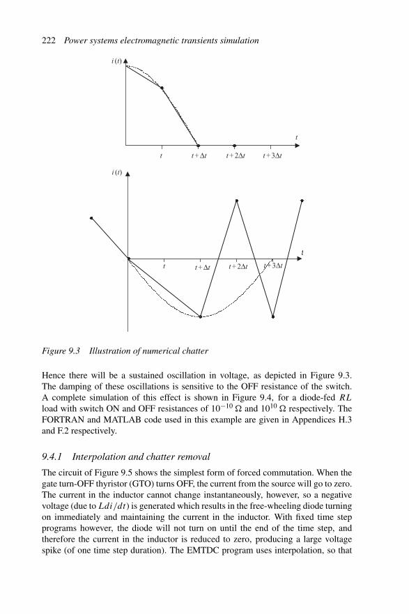
222 Power systems electromagnetic transients simulation
t
i (t)
i (t)
t
t
t
t + Δt
t + Δt
t + 2Δt
t + 2Δt
t + 3Δt
t + 3Δt
Figure 9.3 Illustration of numerical chatter
Hence there will be a sustained oscillation in voltage, as depicted in Figure 9.3.The damping of these oscillations is sensitive to the OFF resistance of the switch.A complete simulation of this effect is shown in Figure 9.4, for a diode-fed RL
load with switch ON and OFF resistances of 10−10 � and 1010 � respectively. TheFORTRAN and MATLAB code used in this example are given in Appendices H.3and F.2 respectively.
9.4.1 Interpolation and chatter removal
The circuit of Figure 9.5 shows the simplest form of forced commutation. When thegate turn-OFF thyristor (GTO) turns OFF, the current from the source will go to zero.The current in the inductor cannot change instantaneously, however, so a negativevoltage (due to Ldi/dt) is generated which results in the free-wheeling diode turningon immediately and maintaining the current in the inductor. With fixed time stepprograms however, the diode will not turn on until the end of the time step, andtherefore the current in the inductor is reduced to zero, producing a large voltagespike (of one time step duration). The EMTDC program uses interpolation, so that
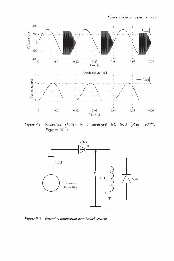
Power electronic systems 223
0 0.01 0.02 0.03 0.04 0.05 0.06
Vol
tage
(vo
lts)
Time (s)
VLoadC
urre
nt (
amps
)
Diode-fed RL load
ILoad
–400
–200
0
200
400
–1
0
1
2
3
Time (s)0 0.01 0.02 0.03 0.04 0.05 0.06
Figure 9.4 Numerical chatter in a diode-fed RL load(RON = 10−10,
ROFF = 1010)
GTO
1.0 Ω
d.c. sourceVDC = 10 V
0.1 H Diode
VL
iL
Figure 9.5 Forced commutation benchmark system
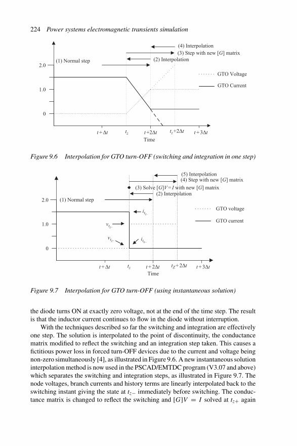
224 Power systems electromagnetic transients simulation
(1) Normal step (2) Interpolation
(4) Interpolation(3) Step with new [G] matrix
Time
GTO Voltage
GTO Current
2.0
1.0
0
t + Δt t +2Δt tz+2Δt t + 3Δttz
Figure 9.6 Interpolation for GTO turn-OFF (switching and integration in one step)
Time
(1) Normal step(2) Interpolation
(5) Interpolation(4) Step with new [G] matrix
(3) Solve [G]V = I with new [G] matrix
vtz– itz–
vtz–
itz–
2.0
1.0
0
GTO voltage
GTO current
t + Δt t + 2Δt tZ+ 2Δt t + 3Δttz
Figure 9.7 Interpolation for GTO turn-OFF (using instantaneous solution)
the diode turns ON at exactly zero voltage, not at the end of the time step. The resultis that the inductor current continues to flow in the diode without interruption.
With the techniques described so far the switching and integration are effectivelyone step. The solution is interpolated to the point of discontinuity, the conductancematrix modified to reflect the switching and an integration step taken. This causes afictitious power loss in forced turn-OFF devices due to the current and voltage beingnon-zero simultaneously [4], as illustrated in Figure 9.6. A new instantaneous solutioninterpolation method is now used in the PSCAD/EMTDC program (V3.07 and above)which separates the switching and integration steps, as illustrated in Figure 9.7. Thenode voltages, branch currents and history terms are linearly interpolated back to theswitching instant giving the state at tz− immediately before switching. The conduc-tance matrix is changed to reflect the switching and [G]V = I solved at tz+ again

Power electronic systems 225
for the instant immediately after switching. From this point the normal integrationstep proceeds. Essentially there are two solutions at every point in which switching isperformed, however these solution points are not written out. Moreover the solutioncan be interpolated numerous times in the same time step to accommodate the mul-tiple switchings that may occur in the same time step. If a non-linear surge arresterchanges state between tz− and tz+ then the solution is interpolated to the discontinuityof the non-linear device, say tz−+. The non-linear device characteristics are changedand then a new tz+ solution obtained, giving three solutions all at time tz.
Ideally what should be kept constant from tz− to tz+ are the inductor current andcapacitor voltage. However, this would require changing the conductance matrix.Instead, the present scheme keeps the current source associated with inductors andcapacitors constant, as the error associated with this method is very small.
Early techniques for overcoming these numerical problems was the insertion ofadditional damping, either in the form of external fictitious resistors (or snubbernetworks) or by the integration rule itself. The former is often justified by the argumentthat in reality the components are not ideal.
The alternative is to use a different integration rule at points of discontinuity.The most widely used technique is critical damping adjustment (CDA), in which theintegration method is changed to the backward Euler for two time steps (of �t/2)after the discontinuity. By using a step size of �t/2 with the backward Euler theconductance matrix is the same as for the trapezoidal rule [5], [6]. The differenceequations for the inductor and capacitor become:
iL
(tZ + �t
2
)= �t
2LvL
(tZ + �t
2
)+ iL(tZ−)
vC
(tZ + �t
2
)= 2C
�tvC
(tZ + �t
2
)− 2C
�tvC(tZ−)
(9.9)
This approach is used in the NETOMAC program [7], [8]. With reference toFigure 9.8 below the zero-crossing instant is determined by linear interpolation. All thevariables (including the history terms) are interpolated back to point tZ . Distinguishingbetween the instants immediately before tZ− and immediately after tZ− switching, theinductive current and capacitor voltages must be continuous across tZ . However, asillustrated in Figure 9.9, the inductor voltage or capacitor current will exhibit jumps.In general the history terms are discontinuous across time. Interpolation is used to findthe voltages and currents as well as the associated history terms. Strictly speaking twotime points should be generated for time tZ one immediately before switching, whichis achieved by this interpolation step, and one immediately after to catch correctlythis jump in voltage and/or current. However, unlike state variable analysis, this isnot performed here. With these values the step is made from tZ to tZ + �t/2 usingthe backward Euler rule. The advantage of using the backward Euler integration stepis that inductor voltages or capacitor currents at tZ+ are not needed. NETOMAC thenuses the calculated inductor voltages or capacitor currents calculated with the half
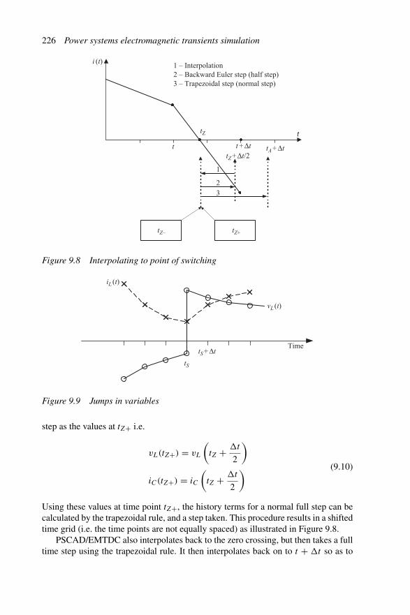
226 Power systems electromagnetic transients simulation
t
ttZ
tZ–
1 – Interpolation2 – Backward Euler step (half step)3 – Trapezoidal step (normal step)
tZ+ Δt/2t + Δt tA+ Δt
tZ+
1
2
3
i (t)
Figure 9.8 Interpolating to point of switching
Time
tS
tS+ Δt
iL (t)
vL (t)
Figure 9.9 Jumps in variables
step as the values at tZ+ i.e.
vL(tZ+) = vL
(tZ + �t
2
)
iC(tZ+) = iC
(tZ + �t
2
) (9.10)
Using these values at time point tZ+, the history terms for a normal full step can becalculated by the trapezoidal rule, and a step taken. This procedure results in a shiftedtime grid (i.e. the time points are not equally spaced) as illustrated in Figure 9.8.
PSCAD/EMTDC also interpolates back to the zero crossing, but then takes a fulltime step using the trapezoidal rule. It then interpolates back on to t + �t so as to

Power electronic systems 227
tZ tZ+ Δtt + Δt
i (t)
t
t
Z
1
2
3
Figure 9.10 Double interpolation method (interpolating back to the switchinginstant)
keep the same time grid, as the post-processing programs expect equally spaced timepoints. This method is illustrated in Figure 9.10 and is known as double interpolationbecause it uses two interpolation steps.
Interpolation has been discussed so far as a method of removing spikes due, forexample, to inductor current chopping. PSCAD/EMTDC also uses interpolation toremove numerical chatter. Chatter manifests itself as a symmetrical oscillation aroundthe true solution; therefore, interpolating back half a time step will give the correctresult and simulation can proceed from this point. Voltage across inductors and currentin capacitors both exhibit numerical chatter. Figure 9.11 illustrates a case where theinductor current becoming zero coincides with a time point (i.e. there is no currentchopping in the inductive circuit). Step 1 is a normal step and step 2 is a half timestep interpolation to the true solution for v(t). Step 3 is a normal step and Step 4 isanother half time step interpolation to get back on to the same time grid.
The two interpolation procedures, to find the switching instant and chatterremoval, are combined into one, as shown in Figure 9.12; this allows the connec-tion of any number of switching devices in any configuration. If the zero crossingoccurs in the second half of the time step (not shown in the figure) this procedure hasto be slightly modified. A double interpolation is first performed to return on to theregular time grid (at t + �t) and then a half time step interpolation performed afterthe next time step (to t + 2�t) is taken. The extra solution points are kept internal toEMTDC (not written out) so that only equal spaced data points are in the output file.
PSCAD/EMTDC invokes the chatter removal algorithm immediately wheneverthere is a switching operation. Moreover the chatter removal detection looks foroscillation in the slope of the voltages and currents for three time steps and, if detected,implements a half time-step interpolation. This detection is needed, as chatter can be
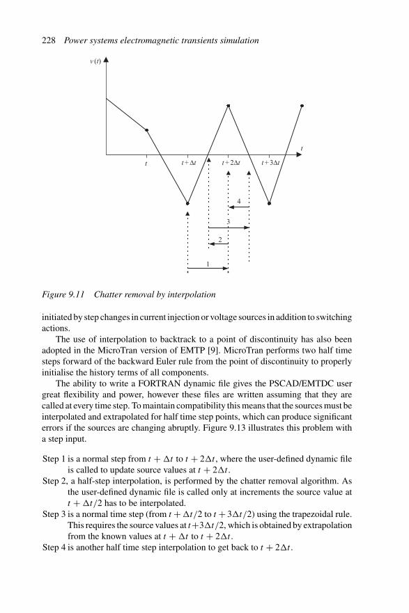
228 Power systems electromagnetic transients simulation
t t + Δt t + 2Δt t + 3Δt
t
1
2
3
4
v (t)
Figure 9.11 Chatter removal by interpolation
initiated by step changes in current injection or voltage sources in addition to switchingactions.
The use of interpolation to backtrack to a point of discontinuity has also beenadopted in the MicroTran version of EMTP [9]. MicroTran performs two half timesteps forward of the backward Euler rule from the point of discontinuity to properlyinitialise the history terms of all components.
The ability to write a FORTRAN dynamic file gives the PSCAD/EMTDC usergreat flexibility and power, however these files are written assuming that they arecalled at every time step. To maintain compatibility this means that the sources must beinterpolated and extrapolated for half time step points, which can produce significanterrors if the sources are changing abruptly. Figure 9.13 illustrates this problem witha step input.
Step 1 is a normal step from t + �t to t + 2�t , where the user-defined dynamic fileis called to update source values at t + 2�t .
Step 2, a half-step interpolation, is performed by the chatter removal algorithm. Asthe user-defined dynamic file is called only at increments the source value att + �t/2 has to be interpolated.
Step 3 is a normal time step (from t + �t/2 to t + 3�t/2) using the trapezoidal rule.This requires the source values at t+3�t/2, which is obtained by extrapolationfrom the known values at t + �t to t + 2�t .
Step 4 is another half time step interpolation to get back to t + 2�t .
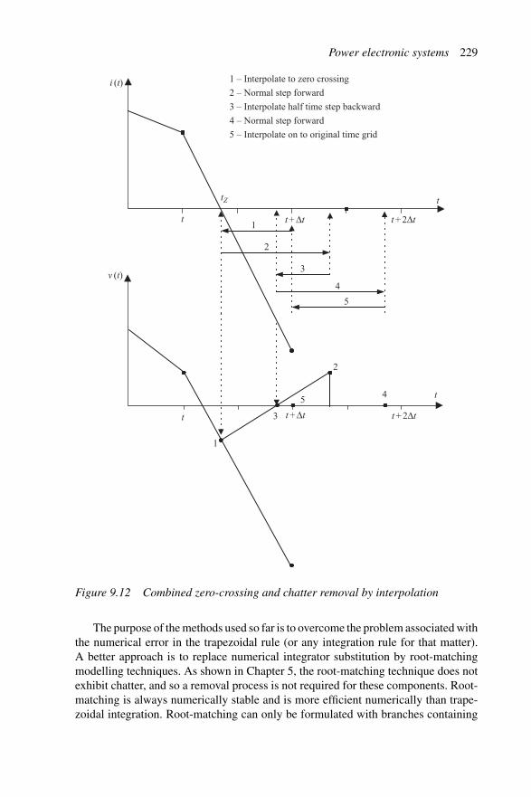
Power electronic systems 229
t
t + Δt
t + Δt
t + 2Δt
t + 2Δt
1
2
3
tZ
t
t
4
5
1
2
3
45
1 – Interpolate to zero crossing
2 – Normal step forward
3 – Interpolate half time step backward
4 – Normal step forward
5 – Interpolate on to original time grid
i (t)
v (t)
t
Figure 9.12 Combined zero-crossing and chatter removal by interpolation
The purpose of the methods used so far is to overcome the problem associated withthe numerical error in the trapezoidal rule (or any integration rule for that matter).A better approach is to replace numerical integrator substitution by root-matchingmodelling techniques. As shown in Chapter 5, the root-matching technique does notexhibit chatter, and so a removal process is not required for these components. Root-matching is always numerically stable and is more efficient numerically than trape-zoidal integration. Root-matching can only be formulated with branches containing

230 Power systems electromagnetic transients simulation
t
Input
t
1
2
4
3
Step input
Userdynamics file
called
Userdynamics file
called
t + Δt t + 2Δt t + 3Δt
t + 3Δt/2t + Δt/2
Interpolatedsource values
Extrapolatedsource values
Figure 9.13 Interpolated/extrapolated source values due to chatter removalalgorithm
two or more elements (i.e. RL, RC, RLC, LC, . . .) but these branches can be inter-mixed in the same solution with branches solved with other integration techniques.
9.5 HVDC converters
PSCAD/EMTDC provides as a single component a six-pulse valve group, shownin Figure 9.14(a), with its associate PLO (Phase Locked Oscillator) firing controland sequencing logic. Each valve is modelled as an off/on resistance, with forwardvoltage drop and parallel snubber, as shown in Figure 9.14(b). The combination of on-resistance and forward-voltage drop can be viewed as a two-piece linear approxima-tion to the conduction characteristic. The interpolated switching scheme, describedin section 9.4.1 (Figure 9.10), is used for each valve.
The LDU factorisation scheme used in EMTDC is optimised for the type ofconductance matrix found in power systems in the presence of frequently switchedelements. The block diagonal structure of the conductance matrix, caused by atravelling-wave transmission line and cable models, is exploited by processing eachassociated subsystem separately and sequentially. Within each subsystem, nodes towhich frequently switched elements are attached are ordered last, so that the matrixrefactorisation after switching need only proceed from the switched node to the end.Nodes involving circuit breakers and faults are not ordered last, however, since they

Power electronic systems 231
Ron Cd
Rd
Roff
Efwd
1 3 5
4 6 2
(a) (b)
abc
+–
Figure 9.14 (a) The six-pulse group converter, (b) thyristor and snubber equivalentcircuit
V�
Vcos
Vsin
VA
�0 �
1.2 �0
0.8 �0GI
1.0
Resetat 2π
+
++
2 ph
3 ph
VB
VC
Vb
+
+
X
X
S
S
GP
Figure 9.15 Phase-vector phase-locked oscillator
switch only once or twice in the course of a simulation. This means that the matrixrefactorisation time is affected mainly by the total number of switched elements in asubsystem, and not by the total size of the subsystem. Sparse matrix indexing methodsare used to process only the non-zero elements in each subsystem. A further speedimprovement, and reduction in algorithmic complexity, are achieved by storing theconductance matrix for each subsystem in full form, including the zero elements. Thisavoids the need for indirect indexing of the conductance matrix elements by meansof pointers.
Although the user has the option of building up a valve group from individualthyristor components, the use of the complete valve group including sequencing andfiring control logic is a better proposition.
The firing controller implemented is of the phase-vector type, shown inFigure 9.15, which employs trigonometric identities to operate on an error signalfollowing the phase of the positive sequence component of the commutating voltage.The output of the PLO is a ramp, phase shifted to account for the transformer phase
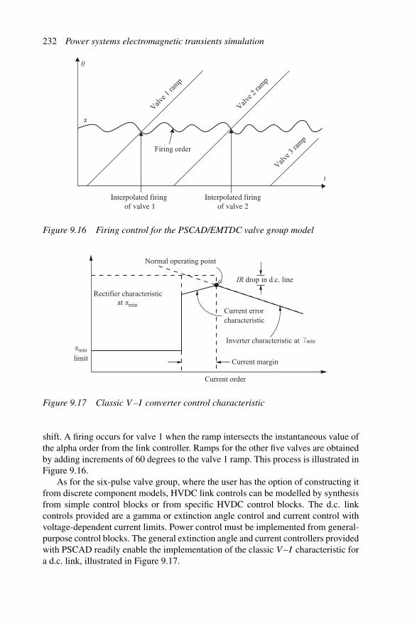
232 Power systems electromagnetic transients simulation
Interpolated firingof valve 1
Interpolated firing of valve 2
Valve 1
ram
p
Valve 2
ram
p
Valve 3
ram
pFiring order
t
�
Figure 9.16 Firing control for the PSCAD/EMTDC valve group model
�min�min
at �min
Current order
Current margin
Current errorcharacteristic
Normal operating point
IR drop in d.c. line
Inverter characteristic at
limit
Rectifier characteristic
Figure 9.17 Classic V –I converter control characteristic
shift. A firing occurs for valve 1 when the ramp intersects the instantaneous value ofthe alpha order from the link controller. Ramps for the other five valves are obtainedby adding increments of 60 degrees to the valve 1 ramp. This process is illustrated inFigure 9.16.
As for the six-pulse valve group, where the user has the option of constructing itfrom discrete component models, HVDC link controls can be modelled by synthesisfrom simple control blocks or from specific HVDC control blocks. The d.c. linkcontrols provided are a gamma or extinction angle control and current control withvoltage-dependent current limits. Power control must be implemented from general-purpose control blocks. The general extinction angle and current controllers providedwith PSCAD readily enable the implementation of the classic V –I characteristic fora d.c. link, illustrated in Figure 9.17.
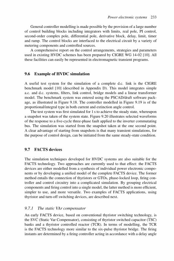
Power electronic systems 233
General controller modelling is made possible by the provision of a large numberof control building blocks including integrators with limits, real pole, PI control,second-order complex pole, differential pole, derivative block, delay, limit, timerand ramp. The control blocks are interfaced to the electrical circuit by a variety ofmetering components and controlled sources.
A comprehensive report on the control arrangements, strategies and parametersused in existing HVDC schemes has been prepared by CIGRE WG 14-02 [10]. Allthese facilities can easily be represented in electromagnetic transient programs.
9.6 Example of HVDC simulation
A useful test system for the simulation of a complete d.c. link is the CIGREbenchmark model [10] (described in Appendix D). This model integrates simplea.c. and d.c. systems, filters, link control, bridge models and a linear transformermodel. The benchmark system was entered using the PSCAD/draft software pack-age, as illustrated in Figure 9.18. The controller modelled in Figure 9.19 is of theproportional/integral type in both current and extinction angle control.
The test system was first simulated for 1 s to achieve the steady state, whereupona snapshot was taken of the system state. Figure 9.20 illustrates selected waveformsof the response to a five-cycle three-phase fault applied to the inverter commutatingbus. The simulation was started from the snapshot taken at the one second point.A clear advantage of starting from snapshots is that many transient simulations, forthe purpose of control design, can be initiated from the same steady-state condition.
9.7 FACTS devices
The simulation techniques developed for HVDC systems are also suitable for theFACTS technology. Two approaches are currently used to that effect: the FACTSdevices are either modelled from a synthesis of individual power electronic compo-nents or by developing a unified model of the complete FACTS device. The formermethod entails the connection of thyristors or GTOs, phase-locked loop, firing con-troller and control circuitry into a complicated simulation. By grouping electricalcomponents and firing control into a single model, the latter method is more efficient,simpler to use, and more versatile. Two examples of FACTS applications, usingthyristor and turn-off switching devices, are described next.
9.7.1 The static VAr compensator
An early FACTS device, based on conventional thyristor switching technology, isthe SVC (Static Var Compensator), consisting of thyristor switched capacitor (TSC)banks and a thyristor controlled reactor (TCR). In terms of modelling, the TCRis the FACTS technology more similar to the six-pulse thyristor bridge. The firinginstants are determined by a firing controller acting in accordance with a delay angle

234 Power systems electromagnetic transients simulation
1.0E6
0.49
7333
2.5
1.0E6
0.49
7333
2.5
21.66667
KB
AR
S GRS
AR
D GRD
DC
RC
DC
MP
DC
IC
DCIMP
DCRMP
NAR
NBR
NCR
AMISAMID
A
B
C
A
B
C
A
B
C
A
B
C
CM
RC
MI
MP
VV
DC
RC
VD
CIC
NA
I
NB
I
NC
I
CM
IX
CM
RX
MP
VX
CM
I
CM
R
MP
V
VRC
VRB
VRA
VR
A
VR
B
VR
C
A B C
AM
GM K
B
Com
Bus
AO
13
5
46
2
A B C
AM
GM K
B
Com
Bus
AO
13
5
46
2
A B C
Com
Bus 4
62
13
5
A B C
Com
Bus 4
62
13
5
TIM
E
GM
ES
GM
ID
GM
IS
Min
D E
A B C
Tm
va =
603
.73
345.
021
3.45
57
#1#2
A B C
A B C
Tm
va =
603
.73
345.
021
3.45
57
#1#2
A B C
A B C
Tm
va =
591
.79
230.
020
9.22
88
#1#2
A B C
A B C
Tm
va =
591
.79
230.
020
9.22
88
#1#2
1.0
1.0
1.0
1.0
1.0
1.0
3.737
3.737
3.737
A
B
C
0.7406
0.74060.0365
0.0365
24.81
24.81
24.81
0.0365
0.0365
0.0365
0.74060.0365
A
B
C
74.286.685
74.28
261.87
6.685
15.04
15.04
15.04
74.286.685
1.671
3.342
3.342
FA
UL
TS
LO
GIC
FA
UL
TT
IME
D
VD
CIC
VD
CR
C
IR1A
IR1B
IR1C
CBA
IR1C
IR1B
IR1A
6.685
6.685
6.685
83.32
0.0136
83.32
0.0136
0.0136
83.32
.1364
261.87
.1364
261.87
.1364
29.76
29.76
29.76
0.151
2160.633
0.151
2160.633
0.151
2160.633
0.7406
0.7406
0.7406
167.213.23
167.213.23
167.213.23
116.38
116.38
116.38
0.0606
0.0606
0.0606
37.03
0.0061
37.03
0.0061
37.03
0.0061
15.04
15.04
15.04
7.522
7.522
7.522
ABC
KB
AO
AM
GM
AM
GM KB
AO
AO
RA
OI
Figure 9.18 CIGRE benchmark model as entered into the PSCAD draft software

Power electronic systems 235
CM
RX
CM
IX
MP
VX
GM
ES
Min
in
1 C
ycle
0.1
3.14
1590
0.26
180
AO
R
AO
I
CM
RS
CM
IS
CO
RD
CE
RR
I
CE
RR
R
CM
AR
G
CE
RR
IMC
NL
G
VD
CL
MP
VS
GM
ES
S
DG
EI
GM
IN
GE
RR
IG
NL
GB
ET
AIG
BE
TA
IC
BE
TA
RB
ET
AR
L
PI
BE
TA
I
G1
+sT G
1 +
sT
G1
+ s
T
Max
D
E
D–
F+
D–
F +
B –
D+
F–
B +
D–
F+
D–
F +
D–
F+IP IP
IP
TIM
E
Arc
Cos
D–
F+
Arc
Cos
L
inea
rise
r
1.0
*0.
6366
1977
Figure 9.19 Controller for the PSCAD/EMTDC simulation of the CIGRE bench-mark model
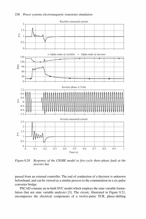
236 Power systems electromagnetic transients simulationp.
u.de
gs
Alpha order @ rectifier Alpha order @ inverterr
p.u.
p.u.
0
0.5
1
1.5
2
0
30
60
90
120
150
–1.2
–0.8
–0.4
0
0.4
0.8
1.2
0
0.5
1
1.5
2
2.5
Rectifier measured current
Inverter phase A Volts
Time (s)
Inverter measured current
0 0.1 0.2 0.3 0.4 0.5 0.6 0.7 0.8 0.9 1
Figure 9.20 Response of the CIGRE model to five-cycle three-phase fault at theinverter bus
passed from an external controller. The end of conduction of a thyristor is unknownbeforehand, and can be viewed as a similar process to the commutation in a six-pulseconverter bridge.
PSCAD contains an in-built SVC model which employs the state variable formu-lation (but not state variable analysis) [3]. The circuit, illustrated in Figure 9.21,encompasses the electrical components of a twelve-pulse TCR, phase-shifting
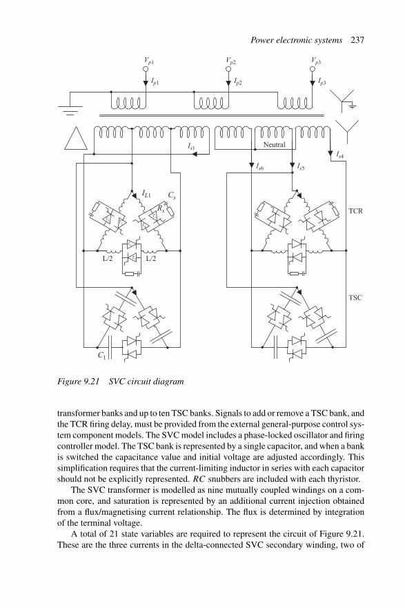
Power electronic systems 237
Vp1 Vp2 Vp3
Ip2 Ip3Ip1
Is1
IL1 Cs
C1
T1
T3
T6
T2 T4
T5
Rs
Is6 Is5
Is4
TCR
TSC
L/2 L/2
Neutral
Figure 9.21 SVC circuit diagram
transformer banks and up to ten TSC banks. Signals to add or remove a TSC bank, andthe TCR firing delay, must be provided from the external general-purpose control sys-tem component models. The SVC model includes a phase-locked oscillator and firingcontroller model. The TSC bank is represented by a single capacitor, and when a bankis switched the capacitance value and initial voltage are adjusted accordingly. Thissimplification requires that the current-limiting inductor in series with each capacitorshould not be explicitly represented. RC snubbers are included with each thyristor.
The SVC transformer is modelled as nine mutually coupled windings on a com-mon core, and saturation is represented by an additional current injection obtainedfrom a flux/magnetising current relationship. The flux is determined by integrationof the terminal voltage.
A total of 21 state variables are required to represent the circuit of Figure 9.21.These are the three currents in the delta-connected SVC secondary winding, two of
238 Power systems electromagnetic transients simulation
tx
IL
Δt
tB
Dt
tA1
Symbol Description
Δt
Dt
�t
Original EMTDC time step
SVC time step
Catch-up time step
�t �t �t
Δt
Switch-OFFoccurs
Time
tA tA2 tA3
Figure 9.22 Thyristor switch-OFF with variable time step
the currents in the ungrounded star-connected secondary, two capacitor voltages ineach of the two delta-connected TSCs (four variables) and the capacitor voltage oneach of the back-to-back thyristor snubbers (4 × 3 = 12 state variables).
The system matrix must be reformed whenever a thyristor switches. Accuratedetermination of the switching instants is obtained by employing an integration steplength which is a submultiple of that employed in the EMTDC main loop. The detec-tion of switchings proceeds as in Figure 9.22. Initially the step length is the same asthat employed in EMTDC. Upon satisfying an inequality that indicates that a switch-ing has occurred, the SVC model steps back a time step and integrates with a smallertime step, until the inequality is satisfied again. At this point the switching is brack-eted by a smaller interval, and the system matrix for the SVC is reformed with thenew topology. A catch-up step is then taken to resynchronise the SVC model withEMTDC, and the step length is increased back to the original.
The interface between the EMTDC and SVC models is by Norton and Theveninequivalents as shown in Figure 9.23. The EMTDC network sees the SVC as a cur-rent source in parallel with a linearising resistance Rc. The linearising resistance isnecessary, since the SVC current injection is calculated by the model on the basis ofthe terminal voltage at the previous time step. Rc is then an approximation to howthe SVC current injection will vary as a function of the terminal voltage value to becalculated at the current time step. The total current flowing in this resistance may be
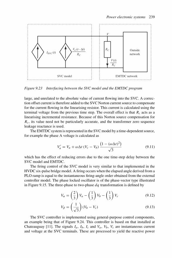
Power electronic systems 239
RC
RC
RC
V
ISVC (t)VC (t – Δt)
V (t)
Outsidenetwork
EMTDC networkSVC model
Figure 9.23 Interfacing between the SVC model and the EMTDC program
large, and unrelated to the absolute value of current flowing into the SVC. A correc-tion offset current is therefore added to the SVC Norton current source to compensatefor the current flowing in the linearising resistor. This current is calculated using theterminal voltage from the previous time step. The overall effect is that Rc acts as alinearising incremental resistance. Because of this Norton source compensation forRc, its value need not be particularly accurate, and the transformer zero sequenceleakage reactance is used.
The EMTDC system is represented in the SVC model by a time-dependent source,for example the phase A voltage is calculated as
V ′a = Va + ω�t (Vc − Vb)
(1 − (ω�t)2)
√3
(9.11)
which has the effect of reducing errors due to the one time-step delay between theSVC model and EMTDC.
The firing control of the SVC model is very similar to that implemented in theHVDC six-pulse bridge model. A firing occurs when the elapsed angle derived from aPLO ramp is equal to the instantaneous firing-angle order obtained from the externalcontroller model. The phase locked oscillator is of the phase-vector type illustratedin Figure 9.15. The three-phase to two-phase dq transformation is defined by
Vα =(
2
3
)Va −
(1
3
)Vb −
(1
3
)Vc (9.12)
Vβ =(
1√3
)(Vb − Vc) (9.13)
The SVC controller is implemented using general-purpose control components,an example being that of Figure 9.24. This controller is based on that installed atChateauguay [11]. The signals Ia , Ib, Ic and Va , Vb, Vc are instantaneous currentand voltage at the SVC terminals. These are processed to yield the reactive power

240 Power systems electromagnetic transients simulation
Reactive power measurement
K
60 Hz
fcutoff
= 90 Hz
B
Allocator
BTCR
BSVS
PLLComparator
12
12
Firing pulses
CapacitorON/OFF to
TSC
Vref
Kp
Ki/s
Filtering
ia ib ic Va Vb Vc
VL (magnitude of busbar voltage)
PI regulator
ix
QSVC
droop(3%)
+167 MVA
–100 MVA
Rectification&
Filtering
+ +∑
120 Hz
–
+
∑ ∑
+
+
��
�
→
Figure 9.24 SVC controls
generation of the SVC and the terminal voltage measurement, from which a reactivecurrent measurement is obtained. The SVC current is used to calculate a current-dependent voltage droop, which is added to the measured voltage. The measuredvoltage with droop is then filtered and subtracted from the voltage reference to yielda voltage error, which is acted upon by a PI controller. The PI controller output isa reactive power order for the SVC, which is split into a component from the TSCbanks by means of an allocator, and a vernier component from the TCR (BTCR).A non-linear reference is used to convert the BTCR reactive power demand into afiring order for the TCR firing controller. A hysteresis TSC bank overlap of ten percent is included in the SVC specification.
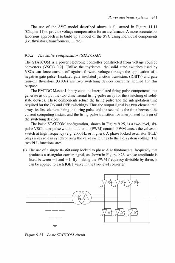
Power electronic systems 241
The use of the SVC model described above is illustrated in Figure 11.11(Chapter 11) to provide voltage compensation for an arc furnace. A more accurate butlaborious approach is to build up a model of the SVC using individual components(i.e. thyristors, transformers, . . . etc).
9.7.2 The static compensator (STATCOM)
The STATCOM is a power electronic controller constructed from voltage sourcedconverters (VSCs) [12]. Unlike the thyristors, the solid state switches used byVSCs can force current off against forward voltage through the application of anegative gate pulse. Insulated gate insulated junction transistors (IGBTs) and gateturn-off thyristors (GTOs) are two switching devices currently applied for thispurpose.
The EMTDC Master Library contains interpolated firing pulse components thatgenerate as output the two-dimensional firing-pulse array for the switching of solid-state devices. These components return the firing pulse and the interpolation timerequired for the ON and OFF switchings. Thus the output signal is a two-element realarray, its first element being the firing pulse and the second is the time between thecurrent computing instant and the firing pulse transition for interpolated turn-on ofthe switching devices.
The basic STATCOM configuration, shown in Figure 9.25, is a two-level, six-pulse VSC under pulse width modulation (PWM) control. PWM causes the valves toswitch at high frequency (e.g. 2000 Hz or higher). A phase locked oscillator (PLL)plays a key role in synchronising the valve switchings to the a.c. system voltage. Thetwo PLL functions are:
(i) The use of a single 0–360 ramp locked to phase A at fundamental frequency thatproduces a triangular carrier signal, as shown in Figure 9.26, whose amplitude isfixed between −1 and +1. By making the PWM frequency divisible by three, itcan be applied to each IGBT valve in the two-level converter.
Figure 9.25 Basic STATCOM circuit

242 Power systems electromagnetic transients simulation
*Modulo360.0
A
B
CCarrier signal generation
A – Increases PLL ramp slope to that required by carrierfrequency
B – Restrains ramps to between 0 and 360 degrees at carrier frequency
C – Converts carrier ramps to carrier signals
to
Figure 9.26 Basic STATCOM controller
(ii) The 0–360 ramp signals generated by the six-pulse PLL are applied to generate sinecurves at the designated fundamental frequency. With reference to Figure 9.27, thetwo degrees of freedom for direct control are achieved by– phase-shifting the ramp signals which in turn phase-shift the sine curves (signalshift), and– varying the magnitude of the sine curves (signal Ma).
It is the control of signals Shift and Ma that define the performance of a voltagesource converter connected to an active a.c. system.
The PWM technique requires mixing the carrier signal with the fundamentalfrequency signal defining the a.c. waveshape. PSCAD/EMTDC models both switchon and switch off pulses with interpolated firing to achieve the exact switching instantsbetween calculation steps, thus avoiding the use of very small time steps. The PWMcarrier signal is compared with the sine wave signals and generates the turn-on andturn-off pulses for the switching interpolation.
The STATCOM model described above is used in Chapter 11 to compensate theunbalance and distortion caused by an electric arc furnace; the resulting waveformsfor the uncompensated and compensated cases are shown in Figures 11.10 and 11.12respectively.
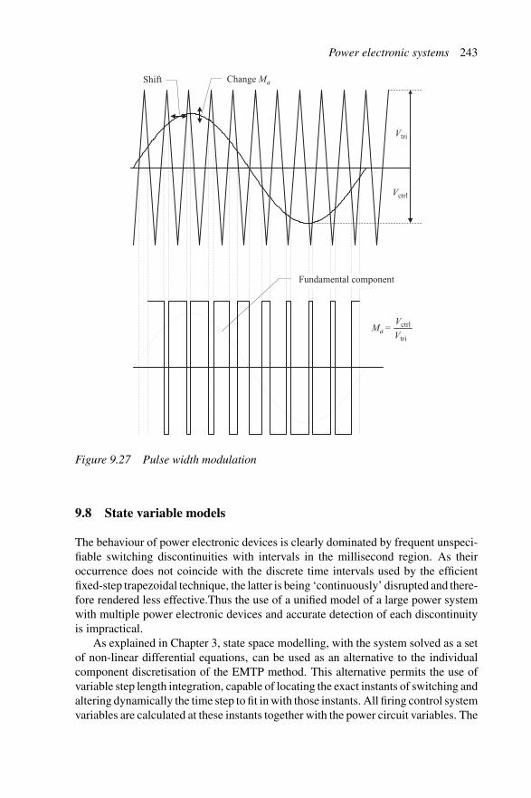
Power electronic systems 243
Vctrl
Vctrl
Ma =Vtri
Vtri
Fundamental component
Change MaShift
Figure 9.27 Pulse width modulation
9.8 State variable models
The behaviour of power electronic devices is clearly dominated by frequent unspeci-fiable switching discontinuities with intervals in the millisecond region. As theiroccurrence does not coincide with the discrete time intervals used by the efficientfixed-step trapezoidal technique, the latter is being ‘continuously’ disrupted and there-fore rendered less effective.Thus the use of a unified model of a large power systemwith multiple power electronic devices and accurate detection of each discontinuityis impractical.
As explained in Chapter 3, state space modelling, with the system solved as a setof non-linear differential equations, can be used as an alternative to the individualcomponent discretisation of the EMTP method. This alternative permits the use ofvariable step length integration, capable of locating the exact instants of switching andaltering dynamically the time step to fit in with those instants. All firing control systemvariables are calculated at these instants together with the power circuit variables. The

244 Power systems electromagnetic transients simulation
solution of the system is iterated at every time step, until convergence is reached withan acceptable tolerance.
Although the state space formulation can handle any topology, the automatic gen-eration of the system matrices and state equations is a complex and time-consumingprocess, which needs to be done every time a switching occurs. Thus the sole useof the state variable method for a large power system is not a practical proposition.Chapter 3 has described TCS [13], a state variable program specially developed forpower electronic systems. This program has provision to include all the non-linearitiesof a converter station (such as transformer magnetisation) and generate automaticallythe comprehensive connection matrices and state space equations of the multicom-ponent system, to produce a continuous state space subsystem. The state variablebased power electronics subsystems can then be combined with the electromagnetictransients program to provide the hybrid solution discussed in the following section.Others have also followed this approach [14].
9.8.1 EMTDC/TCS interface implementation
The system has to be subdivided to represent the components requiring the use of thestate variable formulation [15]. The key to a successful interface is the exclusive use of‘stable’ information from each side of the subdivided system, e.g. the voltage acrossa capacitor and the current through an inductor [16]. Conventional HVDC convertersare ideally suited for interfacing as they possess a stable commutating busbar voltage(a function of the a.c. filter capacitors) and a smooth current injection (a function ofthe smoothing reactor current).
A single-phase example is used next to illustrate the interface technique, whichcan easily be extended to a three-phase case.
The system shown in Figure 9.28 is broken into two subsystems at node M . Thestable quantities in this case are the inductor current for system S1 and the capacitorvoltage for system S2. An interface is achieved through the following relationships
Il Il
Z2
Z1E1I2
Subsystem1
Subsystem2
Subsystem1 Subsystem
2
M
Vc
Vc
(a) (b)
Figure 9.28 Division of a network: (a) network to be divided; (b) divided system
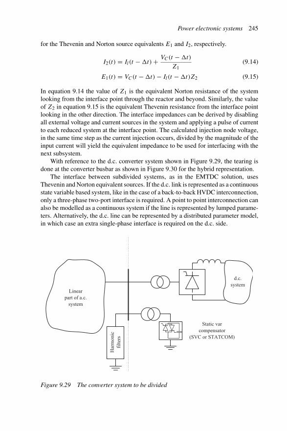
Power electronic systems 245
for the Thevenin and Norton source equivalents E1 and I2, respectively.
I2(t) = Il(t − �t) + VC(t − �t)
Z1(9.14)
E1(t) = VC(t − �t) − Il(t − �t)Z2 (9.15)
In equation 9.14 the value of Z1 is the equivalent Norton resistance of the systemlooking from the interface point through the reactor and beyond. Similarly, the valueof Z2 in equation 9.15 is the equivalent Thevenin resistance from the interface pointlooking in the other direction. The interface impedances can be derived by disablingall external voltage and current sources in the system and applying a pulse of currentto each reduced system at the interface point. The calculated injection node voltage,in the same time step as the current injection occurs, divided by the magnitude of theinput current will yield the equivalent impedance to be used for interfacing with thenext subsystem.
With reference to the d.c. converter system shown in Figure 9.29, the tearing isdone at the converter busbar as shown in Figure 9.30 for the hybrid representation.
The interface between subdivided systems, as in the EMTDC solution, usesThevenin and Norton equivalent sources. If the d.c. link is represented as a continuousstate variable based system, like in the case of a back-to-back HVDC interconnection,only a three-phase two-port interface is required. A point to point interconnection canalso be modelled as a continuous system if the line is represented by lumped parame-ters. Alternatively, the d.c. line can be represented by a distributed parameter model,in which case an extra single-phase interface is required on the d.c. side.
Linearpart of a.c.
system
d.c.system
Static var compensator
(SVC or STATCOM)
Har
mon
icfi
lter
s
Figure 9.29 The converter system to be divided
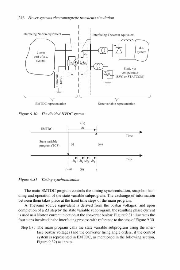
246 Power systems electromagnetic transients simulation
d.c.system
Static var compensator
(SVC or STATCOM)
E1
Z2
Z1
I2
Linearpart of a.c.
system
Interfacing Thevenin equivalentInterfacing Norton equivalent
EMTDC representation State variable representation
Har
mon
icfi
lter
s
Figure 9.30 The divided HVDC system
Δt
�t1 �t2 �t3 �t4
EMTDC
Time
State variable program (TCS)
Time
(i) (iii)
(iv)
(ii) tt – Δt
Figure 9.31 Timing synchronisation
The main EMTDC program controls the timing synchronisation, snapshot han-dling and operation of the state variable subprogram. The exchange of informationbetween them takes place at the fixed time steps of the main program.
A Thevenin source equivalent is derived from the busbar voltages, and uponcompletion of a �t step by the state variable subprogram, the resulting phase currentis used as a Norton current injection at the converter busbar. Figure 9.31 illustrates thefour steps involved in the interfacing process with reference to the case of Figure 9.30.
Step (i) : The main program calls the state variable subprogram using the inter-face busbar voltages (and the converter firing angle orders, if the controlsystem is represented in EMTDC, as mentioned in the following section,Figure 9.32) as inputs.
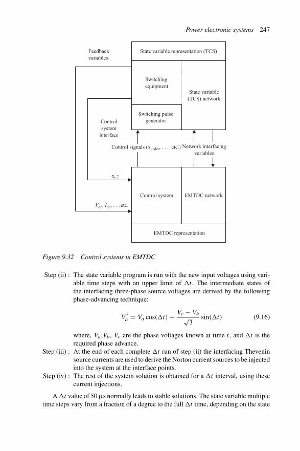
Power electronic systems 247
State variable representation (TCS)
Switching pulse generator
Switchingequipment
State variable (TCS) network
Control system EMTDC network
EMTDC representation
Control signals (�order, . . . etc.) Network interfacing variables
Feedbackvariables
Controlsystem
interface
Vdc, Idc, . . . etc.
�, �
Figure 9.32 Control systems in EMTDC
Step (ii) : The state variable program is run with the new input voltages using vari-able time steps with an upper limit of �t . The intermediate states ofthe interfacing three-phase source voltages are derived by the followingphase-advancing technique:
V ′a = Va cos(�t) + Vc − Vb√
3sin(�t) (9.16)
where, Va ,Vb, Vc are the phase voltages known at time t , and �t is therequired phase advance.
Step (iii) : At the end of each complete �t run of step (ii) the interfacing Theveninsource currents are used to derive the Norton current sources to be injectedinto the system at the interface points.
Step (iv) : The rest of the system solution is obtained for a �t interval, using thesecurrent injections.
A �t value of 50 μs normally leads to stable solutions. The state variable multipletime steps vary from a fraction of a degree to the full �t time, depending on the state
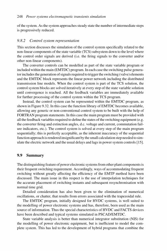
248 Power systems electromagnetic transients simulation
of the system. As the system approaches steady state the number of intermediate stepsis progressively reduced.
9.8.2 Control system representation
This section discusses the simulation of the control system specifically related to thenon-linear components of the state variable (TCS) subsystem down to the level wherethe control order signals are derived (i.e. the firing signals to the converter and/orother non-linear components).
The converter controls can be modelled as part of the state variable program orincluded within the main (EMTDC) program. In each case the switching pulse genera-tor includes the generation of signals required to trigger the switching (valve) elementsand the EMTDC block represents the linear power network including the distributedtransmission line models. When the control system is part of the TCS solution, thecontrol system blocks are solved iteratively at every step of the state variable solutionuntil convergence is reached. All the feedback variables are immediately availablefor further processing of the control system within the TCS program.
Instead, the control system can be represented within the EMTDC program, asshown in Figure 9.32. In this case the function library of EMTDC becomes available,allowing any generic or non-conventional control system to be built with the help ofFORTRAN program statements. In this case the main program must be provided withall the feedback variables required to define the states of the switching equipment (e.g.the converter firing and extinction angles, d.c. voltage and current, commutation fail-ure indicators, etc.). The control system is solved at every step of the main programsequentially; this is perfectly acceptable, as the inherent inaccuracy of the sequentialfunction approach is rendered insignificant by the small calculation step needed to sim-ulate the electric network and the usual delays and lags in power system controls [15].
9.9 Summary
The distinguishing feature of power electronic systems from other plant components istheir frequent switching requirement. Accordingly, ways of accommodating frequentswitching without greatly affecting the efficiency of the EMTP method have beendiscussed. The main issue in this respect is the use of interpolation techniques forthe accurate placement of switching instants and subsequent resynchronisation withnormal time grid.
Detailed consideration has also been given to the elimination of numericaloscillations, or chatter, that results from errors associated with the trapezoidal rule.
The EMTDC program, initially designed for HVDC systems, is well suited tothe modelling of power electronic systems and has, therefore, been used as the mainsource of information. Thus the special characteristics of HVDC and FACTS deviceshave been described and typical systems simulated in PSCAD/EMTDC.
State variable analysis is better than numerical integrator substitution (NIS) forthe modelling of power electronic equipment, but is inefficient to model the com-plete system. This has led to the development of hybrid programs that combine the
Power electronic systems 249
two methods into one program. However, considerable advances have been made inNIS programs to handle frequent switching efficiently and thus the complex hybridmethods are less likely to be widely used.
9.10 References
1 DOMMEL, H. W.: ‘Digital computer solution of electromagnetic transients insingle- and multiphase networks’, IEEE Transactions on Power Apparatus andSystems, 1969, 88 (2), pp. 734–41
2 TINNEY, W. F. and WALKER, J. W.: ‘Direct solutions of sparse network equa-tions by optimally ordered triangular factorization’, Proccedings of IEEE, 1967,55, pp. 1801–9
3 GOLE, A. M. and SOOD, V. K.: ‘A static compensator model for use with electro-magnetic transients simulation programs’, IEEE Transactions on Power Delivery,1990, 5 (3), pp. 1398–1407
4 IRWIN, G. D., WOODFORD, D. A. and GOLE, A.: ‘Precision simulation ofPWM controllers’, Proceedings of International Conference on Power SystemTransients (IPST’2001), June 2001, pp. 161–5
5 LIN, J. and MARTI, J. R.: ‘Implementation of the CDA procedure in EMTP’,IEEE Transactions on Power Systems, 1990, 5 (2), pp. 394–402
6 MARTI, J. R. and LIN, J.: ‘Suppression of numerical oscillations in the EMTP’,IEEE Transactions on Power Systems, 1989, 4 (2), pp. 739–47
7 KRUGER, K. H. and LASSETER, R. H.: ‘HVDC simulation using NETOMAC’,Proceedings, IEEE Montec ’86 Conference on HVDC Power Transmission,Sept/Oct 1986, pp. 47–50
8 KULICKE, B.: ‘NETOMAC digital program for simulating electromechan-ical and electromagnetic transient phenomena in AC power systems’,Elektrizitätswirtschaft, 1, 1979, pp. 18–23
9 ARAUJO, A. E. A., DOMMEL, H. W. and MARTI, J. R.: ‘Converter simulationswith the EMTP: simultaneous solution and backtracking technique’, IEEE/NTUAAthens Power Tech Conference: Planning, Operation and Control of Today’sElectric Power Systems, Sept. 5–8, 1993, 2, pp. 941–5
10 SZECHTMAN, M., WESS, T. and THIO, C. V.: ‘First benchmark model forHVdc control studies’, ELECTRA, 1991, 135, pp. 55–75
11 HAMMAD, A. E.: ‘Analysis of second harmonic instability for the ChateauguayHVdc/SVC scheme’, IEEE Transaction on Power Delivery, 1992, 7 (1),pp. 410–15
12 WOODFORD, D. A.: ‘Introduction to PSCAD/EMTDC V3’, Manitoba HVdcResearch Centre, Canada
13 ARRILLAGA, J., AL-KASHALI, H. J. and CAMPOS-BARROS, J. G.: ‘Generalformulation for dynamic studies in power systems including static converters’,Proceedings of IEE, 1977, 124 (11), pp. 1047–52
14 DAS, B. and GHOSH, A.: ‘Generalised bridge converter model for electro-magnetic transient analysis’, IEE Proc.-Gener. Transm. Distrib., 1998, 145 (4),pp. 423–9

250 Power systems electromagnetic transients simulation
15 ZAVAHIR, J. M., ARRILLAGA, J. and WATSON, N. R.: ‘Hybrid electromag-netic transient simulation with the state variable representation of HVdc converterplant’, IEEE Transactions on Power Delivery, 1993, 8 (3), pp. 1591–8
16 WOODFORD, D. A.: ‘EMTDC users’ manual’, Manitoba HVdc ResearchCentre, Canada
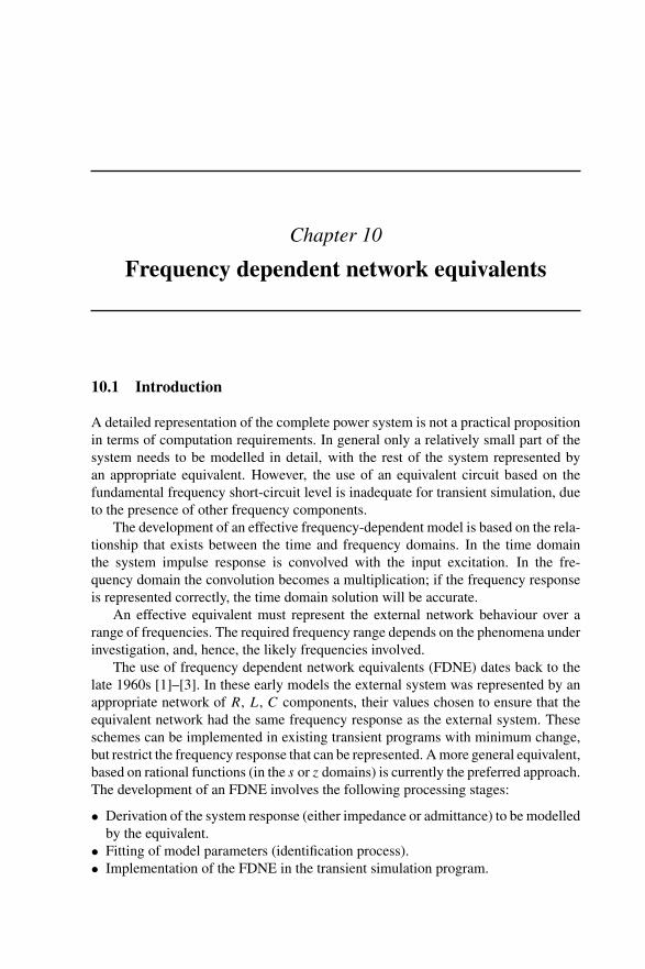
Chapter 10
Frequency dependent network equivalents
10.1 Introduction
A detailed representation of the complete power system is not a practical propositionin terms of computation requirements. In general only a relatively small part of thesystem needs to be modelled in detail, with the rest of the system represented byan appropriate equivalent. However, the use of an equivalent circuit based on thefundamental frequency short-circuit level is inadequate for transient simulation, dueto the presence of other frequency components.
The development of an effective frequency-dependent model is based on the rela-tionship that exists between the time and frequency domains. In the time domainthe system impulse response is convolved with the input excitation. In the fre-quency domain the convolution becomes a multiplication; if the frequency responseis represented correctly, the time domain solution will be accurate.
An effective equivalent must represent the external network behaviour over arange of frequencies. The required frequency range depends on the phenomena underinvestigation, and, hence, the likely frequencies involved.
The use of frequency dependent network equivalents (FDNE) dates back to thelate 1960s [1]–[3]. In these early models the external system was represented by anappropriate network of R, L, C components, their values chosen to ensure that theequivalent network had the same frequency response as the external system. Theseschemes can be implemented in existing transient programs with minimum change,but restrict the frequency response that can be represented. A more general equivalent,based on rational functions (in the s or z domains) is currently the preferred approach.The development of an FDNE involves the following processing stages:
• Derivation of the system response (either impedance or admittance) to be modelledby the equivalent.
• Fitting of model parameters (identification process).• Implementation of the FDNE in the transient simulation program.
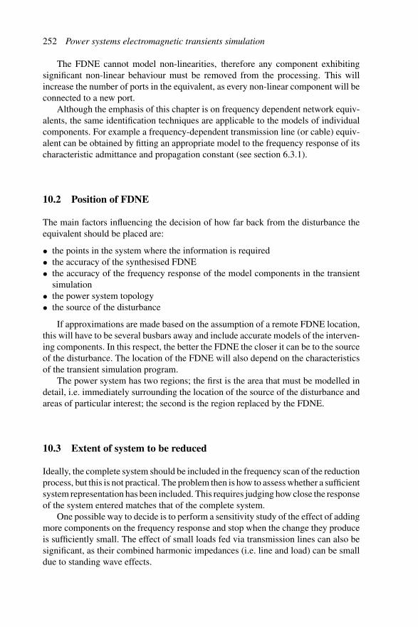
252 Power systems electromagnetic transients simulation
The FDNE cannot model non-linearities, therefore any component exhibitingsignificant non-linear behaviour must be removed from the processing. This willincrease the number of ports in the equivalent, as every non-linear component will beconnected to a new port.
Although the emphasis of this chapter is on frequency dependent network equiv-alents, the same identification techniques are applicable to the models of individualcomponents. For example a frequency-dependent transmission line (or cable) equiv-alent can be obtained by fitting an appropriate model to the frequency response of itscharacteristic admittance and propagation constant (see section 6.3.1).
10.2 Position of FDNE
The main factors influencing the decision of how far back from the disturbance theequivalent should be placed are:
• the points in the system where the information is required• the accuracy of the synthesised FDNE• the accuracy of the frequency response of the model components in the transient
simulation• the power system topology• the source of the disturbance
If approximations are made based on the assumption of a remote FDNE location,this will have to be several busbars away and include accurate models of the interven-ing components. In this respect, the better the FDNE the closer it can be to the sourceof the disturbance. The location of the FDNE will also depend on the characteristicsof the transient simulation program.
The power system has two regions; the first is the area that must be modelled indetail, i.e. immediately surrounding the location of the source of the disturbance andareas of particular interest; the second is the region replaced by the FDNE.
10.3 Extent of system to be reduced
Ideally, the complete system should be included in the frequency scan of the reductionprocess, but this is not practical. The problem then is how to assess whether a sufficientsystem representation has been included. This requires judging how close the responseof the system entered matches that of the complete system.
One possible way to decide is to perform a sensitivity study of the effect of addingmore components on the frequency response and stop when the change they produceis sufficiently small. The effect of small loads fed via transmission lines can also besignificant, as their combined harmonic impedances (i.e. line and load) can be smalldue to standing wave effects.

Frequency dependent network equivalents 253
10.4 Frequency range
The range of the frequency scan and the FDNE synthesis will depend on the problembeing studied. In all cases, however, the frequency scan range should extend beyondthe maximum frequency of the phenomena under investigation. Moreover, the firstresonance above the maximum frequency being considered should also be includedin the scan range, because it will affect the frequency response in the upper part ofthe required frequency range.
Another important factor is the selection of the interval between frequency points,to ensure that all the peaks and troughs are accurately determined. Moreover this willimpact on the number and position of the frequency points used for the calculationof the LSE (least square error) if optimisation techniques are applied. The systemresponse at intermediate points can be found by interpolation; this is computationallymore efficient than the direct determination of the response using smaller intervals.An interval of 5 Hz in conjunction with cubic spline interpolation yields practicallythe same system response derived at 1 Hz intervals, which is perfectly adequate formost applications. However cubic spline interpolation needs to be applied to both thereal and imaginary parts of the system response.
10.5 System frequency response
The starting point in the development of the FDNE is the derivation of the externalsystem driving point and transfer impedance (or admittance) matrices at the boundarybusbar(s), over the frequency range of interest.
Whenever available, experimental data can be used for this purpose, but this israrely the case, which leaves only time or frequency domain identification techniques.When using frequency domain identification, the required data to identify the modelparameters can be obtained either from time or frequency domain simulation, asillustrated in Figure 10.1.
10.5.1 Frequency domain identification
The admittance or impedance seen from a terminal busbar can be calculated fromcurrent or voltage injections, as shown in Figures 10.2 and 10.3 respectively. Theinjections can be performed in the time domain, with multi-sine excitation, or in thefrequency domain, where each frequency is considered independently. The frequencydomain programs can generate any required frequency-dependent admittance as seenfrom the terminal busbars.
Because the admittance (and impedance) matrices are symmetrical, there areonly six different responses to be fitted and these can be determined from threeinjection tests.
When using voltage injections the voltage source and series impedance need tobe made sufficiently large so that the impedance does not adversely affect the maincircuit. If made too small, the conductance term is large and may numerically swamp
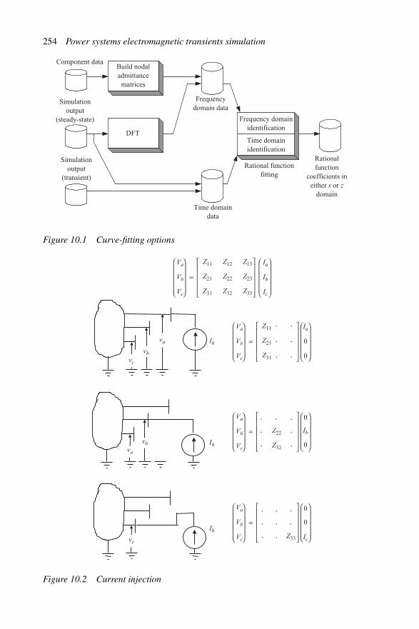
254 Power systems electromagnetic transients simulation
Build nodal admittance
matrices
DFT
Component data
Simulationoutput
(steady-state)
Simulationoutput
(transient)
Frequencydomain data
Time domain data
Rationalfunction
coefficients in either s or z
domain
Rational function fitting
Frequency domain identification
Time domain identification
Figure 10.1 Curve-fitting options
Z13
Z23
Z33
Z12
Z22
Z32
Z11
Z21
Z31
Va
va
va
vc
Vb
vb
vb
Vc
vc
Ia
Ib
Ic
=
Z11
Z21
Z31
Va
Vb
Vc
Ia
Ih
Ih
Ih
0
0
=
. .
. .
. .
Z22
Z32
Va
Vb
Vc
Ib
0
0
=
..
.
.
.
..
Z33
Va
Vb
Vc Ic
0
0=
. ..
. .
.
.
.
Figure 10.2 Current injection
Frequency dependent network equivalents 255
Y13
Y23
Y33
Y12
Y22
Y32
Y11
Y21
Y31
Ia
Ia
Ib
Ib
Ic
Ic
Ib
Ic
Ic
Va
Vb
Vc
=
Y21
Y31
Ib
Ic
Vh
Vh
Vh
0
0
=
. .
. .
. .
Y32
Ia
Ic
0
0
.. .
..
Y33
Ia
Ib
Ic Vc
0
0=
. ..
. .
.
.
.
Y11Ia Va
Y22Ib Vb= . .
Figure 10.3 Voltage injection
out some of the circuit parameters that need to be identified. The use of currentinjections, shown in Figure 10.2, is simpler in this respect.
10.5.1.1 Time domain analysis
Figure 10.4 displays a schematic of a system drawn in DRAFT (PSCAD/EMTDC),where a multi-sine current injection is applied. In this case a range of sine waves isinjected from 5 Hz up to 2500 Hz with 5 Hz spacing; all the magnitudes are 1.0 and theangles 0.0, hence the voltage is essentially the impedance. As the lowest frequencyinjected is 5 Hz all the sine waves add constructively every 0.2 seconds, resulting ina large peak. After the steady state is achieved, one 0.2 sec period is extracted fromthe time domain waveforms, as shown in Figure 10.5, and a DFT performed to obtainthe required frequency response. This frequency response is shown in Figure 10.6.As has been shown in Figure 10.2 the current injection gives the impedances for the

256 Power systems electromagnetic transients simulation
Un
iver
sity
Of
Can
terb
ury
Low
er S
outh
Isl
and
Cre
ated
:L
ast M
odif
ied:
Pri
nted
On::
May
11,
199
8 (m
oa11
)Ja
nuar
y 19
, 199
9 (w
atso
n)M
arch
07,
200
1 (w
atso
n)
SS 1
Inve
rcar
gill
Bus
2 3
5 6
2 3
2 3
2 3
5 6
A
B
C
A
B
C
Tmva = 100.0
220.0 33.0
#1 #2
Tap
1.02
5
9.6276e-2
9.6276e-2
9.6276e-2
EIn
vB
EIn
vA
EIn
vA
EIn
vB
EIn
vC
A B C
A B C
RR
L
RR
L
RR
L
A B C
RR
L
RR
L
RR
L
A B C
E1
RM
SQ
2OU
T
RM
SP
2OU
T
E2
E2
RM
S
Man
apou
riB
us
E1
RM
S
RM
SP
OU
T
RM
SQ
OU
T
tiw
ai 1
2 3
5 6
invc
arg
25
A
B
C
A
B
C
Tmva = 100.0
14.0 220.0
#1 #2
Tap
1.02
5
A
B
C
A
B
C14.0 220.0
#1 #2
Tap
1.02
5
Rox
burg
hB
us
roxb
11 2 3
A
B
C
A
B
C
Tmva = 100.0
11.0 220.0
#1 #2
Tap
RR
L
RR
L
RR
L
A B C
A B C
roxb
21 2 3
1.02
5
1.02
5
A
B
C
A
B
C
Tmva = 100.0
220.0 11.0
#1 #2
Tap
7.1316e-3
7.1316e-3
7.1316e-3
Em
an B
Em
an C
Em
an A
ER
oxA
ER
oxB
ER
oxC
Em
an A
Em
an B
Em
an C
tiw
ai2
1 2 3
4 5 6
tiw
ai1
1 2 3
4 5 6
Tiw
ai
Bus
Har
mon
ic
Cur
rent
Inje
ctio
n
0.00
1
0.00
1
0.00
1
Ib Ic
Pha
se C
Pha
se B
Ia
Pha
se A
Pha
se A
Pha
se B
Pha
se C
Ia Ib Ic
IaAU
TO
GA
IN (1)
(2)
(3)
(4)
(5)
(6)
Ib Ic
Pha
se A
Pha
se B
A B C
11
14
14
invc
arg
roxb
2ro
xb1
tiw
ai2
EIn
vC
Tmva = 100.0
14
36
14
ER
oxB
ER
oxC
ER
oxA
8.066
8.066
8.066
1.3444
1.3444
1.3444
Figure 10.4 PSCAD/EMTDC schematic with current injection
submatrices. In the cases of a single port this is simply inverted; however in the moregeneral multiport case the impedance matrix must be built and then a matrix inversionperformed.
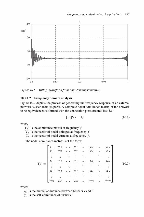
Frequency dependent network equivalents 257
×103
Vc
–30
–10
10
30
50
0.8 0.85 0.9 0.95 1
Figure 10.5 Voltage waveform from time domain simulation
10.5.1.2 Frequency domain analysis
Figure 10.7 depicts the process of generating the frequency response of an externalnetwork as seen from its ports. A complete nodal admittance matrix of the networkto be equivalenced is formed with the connection ports ordered last, i.e.
[Yf ]Vf = If (10.1)
where[Yf ] is the admittance matrix at frequency f
Vf is the vector of nodal voltages at frequency f
If is the vector of nodal currents at frequency f .
The nodal admittance matrix is of the form:
[Yf ] =
⎡
⎢⎢⎢⎢⎢⎢⎢⎢⎢⎢⎢⎢⎢⎣
y11 y12 . . . y1i . . . y1k . . . y1N
y21 y22 . . . y2i . . . y2k . . . y2N
......
. . ....
. . ....
. . ....
yi1 yi2 . . . yii . . . yik . . . yiN
......
. . ....
. . ....
. . ....
yk1 yk2 . . . yki . . . ykk . . . ykN
......
. . ....
. . ....
. . ....
yN1 yN2 . . . yNi . . . yNk . . . yNN
⎤
⎥⎥⎥⎥⎥⎥⎥⎥⎥⎥⎥⎥⎥⎦
(10.2)
whereyki is the mutual admittance between busbars k and i
yii is the self-admittance of busbar i.
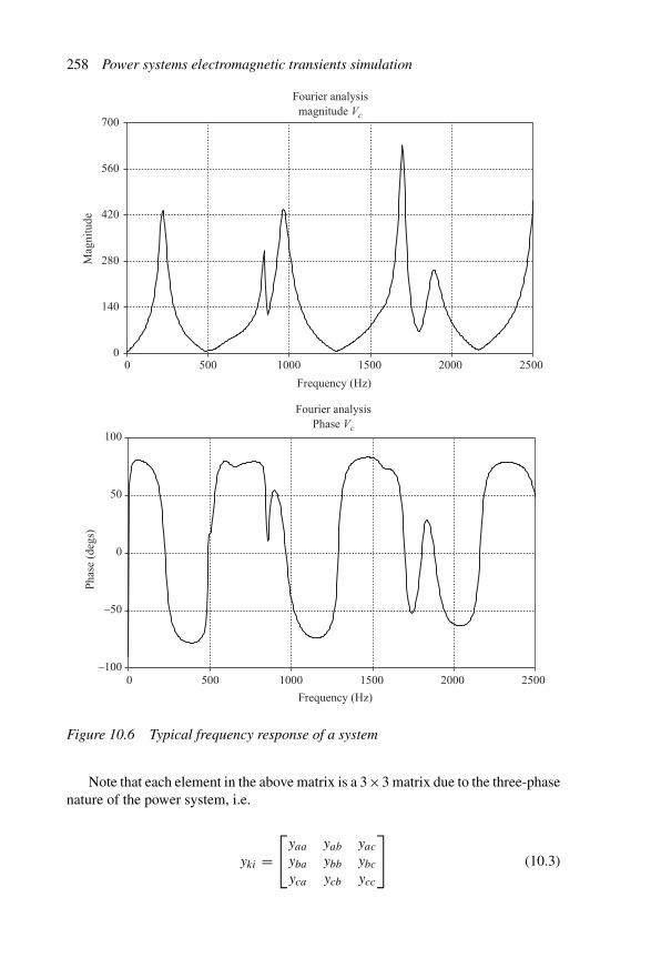
258 Power systems electromagnetic transients simulation
Mag
nitu
deFourier analysis magnitude Vc
Pha
se (
degs
)
Frequency (Hz)
Fourier analysis Phase Vc
0
140
280
420
560
700
Frequency (Hz)
0 500 1000 1500 2000 2500
–100
–50
0
50
100
0 500 1000 1500 2000 2500
Figure 10.6 Typical frequency response of a system
Note that each element in the above matrix is a 3×3 matrix due to the three-phasenature of the power system, i.e.
yki =⎡
⎣yaa yab yac
yba ybb ybc
yca ycb ycc
⎤
⎦ (10.3)

Frequency dependent network equivalents 259
y�11
y11 y12 y1n
y21
yn1ykk ykN
yNNyNk
y22
y2n
y2n
ynn
y�11
y�21
y�31
y�12
y�12 y�1N
y�22
y�22
y�32
y�13
y�23
y�33
y�33
y�1N
y�2N
y�3N
y�NNy�N3y�N2y�N1
...
...
...
...
...
...
......
...
.... . .
. . .
. . .
. . .. . .
. . . . . . . . . . . . . . .
......
...
0
0
0
0
0
0
0
. . .
. . .
. . .
. . .
. . .
. . .
. . .
. . .
. . .
. . .
. . . . . .
...
...
...
0
0
Port n
Port 1
Port 2
n – Number of ports
k = N – n + 1
N – Number of nodes
Figure 10.7 Reduction of admittance matrices
Gaussian elimination is performed on the matrix shown in 10.2, up to, but notincluding the connection ports i.e.
⎡
⎢⎢⎢⎢⎢⎢⎢⎢⎢⎢⎢⎣
y′11 y′
12 . . . . . . y′1k . . . y′
1N
0 y′22 y′
23 . . . y′2k y′
2N
0 0 y′33 y′
34 y′3k y′
3N...
.... . .
. . ....
...
0 0 . . . 0 y′′kk . . . y′′
kN...
... . . . 0...
. . ....
0 0 . . . 0 y′′Nk
. . . y′′NN
⎤
⎥⎥⎥⎥⎥⎥⎥⎥⎥⎥⎥⎦
(10.4)
The matrix equation based on the admittance matrix 10.4 is of the form:
[[yA] [yB ]0 [yD]
] [Vinternal
Vterminal
]=
[0
Iterminal
](10.5)
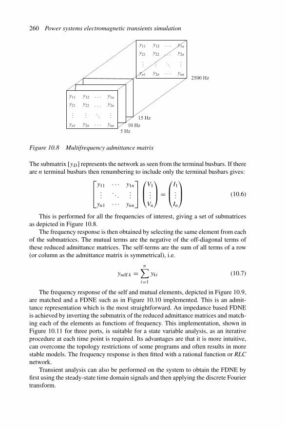
260 Power systems electromagnetic transients simulation
2500 Hz
5 Hz10 Hz
15 Hz
y11 y12 y1n
y21
yn1
y22
y2n
y2n
ynn
......
.... . .
. . .
. . .
. . .
y11 y12 y1n
y21
yn1
y22
y2n
y2n
ynn
......
.... . .
. . .
. . .
. . .
Figure 10.8 Multifrequency admittance matrix
The submatrix [yD] represents the network as seen from the terminal busbars. If thereare n terminal busbars then renumbering to include only the terminal busbars gives:
⎡
⎢⎣
y11 · · · y1n
.... . .
...
yn1 · · · ynn
⎤
⎥⎦
⎛
⎜⎝
V1...
Vn
⎞
⎟⎠ =
⎛
⎜⎝
I1...
In
⎞
⎟⎠ (10.6)
This is performed for all the frequencies of interest, giving a set of submatricesas depicted in Figure 10.8.
The frequency response is then obtained by selecting the same element from eachof the submatrices. The mutual terms are the negative of the off-diagonal terms ofthese reduced admittance matrices. The self-terms are the sum of all terms of a row(or column as the admittance matrix is symmetrical), i.e.
yself k =n∑
i=1
yki (10.7)
The frequency response of the self and mutual elements, depicted in Figure 10.9,are matched and a FDNE such as in Figure 10.10 implemented. This is an admit-tance representation which is the most straightforward. An impedance based FDNEis achieved by inverting the submatrix of the reduced admittance matrices and match-ing each of the elements as functions of frequency. This implementation, shown inFigure 10.11 for three ports, is suitable for a state variable analysis, as an iterativeprocedure at each time point is required. Its advantages are that it is more intuitive,can overcome the topology restrictions of some programs and often results in morestable models. The frequency response is then fitted with a rational function or RLCnetwork.
Transient analysis can also be performed on the system to obtain the FDNE byfirst using the steady-state time domain signals and then applying the discrete Fouriertransform.
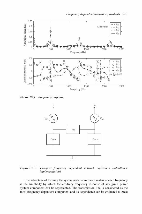
Frequency dependent network equivalents 261
Frequency (Hz)
Adm
itta
nce
mag
nitu
de y11y12y13
y�11
Frequency (Hz)
Adm
itta
nce
phas
e an
gle
Line styles
Markers
0
0.05
0.1
0.15
0.2
0.25
0 500 1000 1500 2000 2500
–100
0
100
200
–2000 500 1000 1500 2000 2500
y11y12y13
y�11
Figure 10.9 Frequency response
1 2
Voc1
–y12
yself 2yself 1
Voc2
Figure 10.10 Two-port frequency dependent network equivalent (admittanceimplementation)
The advantage of forming the system nodal admittance matrix at each frequencyis the simplicity by which the arbitrary frequency response of any given powersystem component can be represented. The transmission line is considered as themost frequency-dependent component and its dependence can be evaluated to great

262 Power systems electromagnetic transients simulation
Z12 I2 + Z13 I3
Z21 I1 + Z23 I3
Z31 I1 + Z32 I2
I1
I2Z11
Z22
Z33
I3
Figure 10.11 Three-phase frequency dependent network equivalent (impedanceimplementation)
accuracy. Other power system components are not modelled to the same accuracy atpresent due to lack of detailed data.
10.5.2 Time domain identification
Model identification can also be performed directly from time domain data. However,in order to identify the admittance or impedance at a particular frequency there mustbe a source of that frequency component. This source may be a steady-state type asin a multi-sine injection [4], or transient such as the ring down that occurs after adisturbance. Prony analysis (described in Appendix B) is the identification techniqueused for the ring down alternative.
10.6 Fitting of model parameters
10.6.1 RLC networks
The main reason for realising an RLC network is the simplicity of its implementionin existing transient analysis programs without requiring extensive modifications.
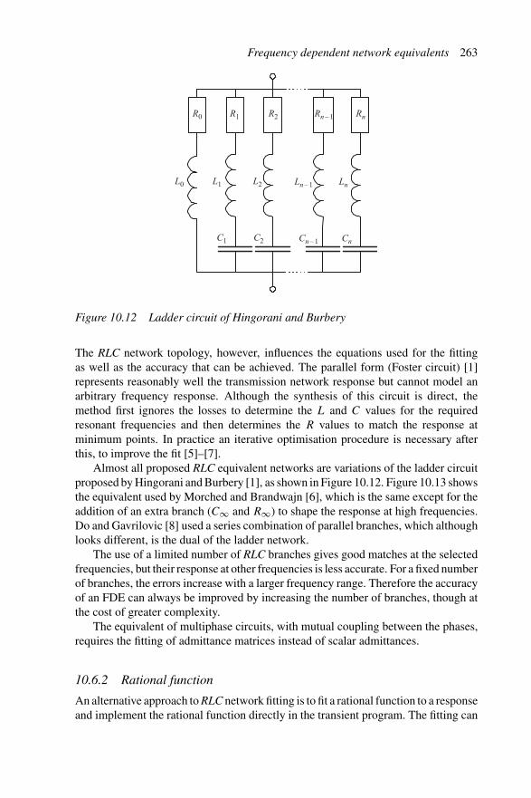
Frequency dependent network equivalents 263
R0 R1
L0 L1 L2
C1 C2
Rn – 1
Ln – 1 Ln
Cn – 1 Cn
R2 Rn
Figure 10.12 Ladder circuit of Hingorani and Burbery
The RLC network topology, however, influences the equations used for the fittingas well as the accuracy that can be achieved. The parallel form (Foster circuit) [1]represents reasonably well the transmission network response but cannot model anarbitrary frequency response. Although the synthesis of this circuit is direct, themethod first ignores the losses to determine the L and C values for the requiredresonant frequencies and then determines the R values to match the response atminimum points. In practice an iterative optimisation procedure is necessary afterthis, to improve the fit [5]–[7].
Almost all proposed RLC equivalent networks are variations of the ladder circuitproposed by Hingorani and Burbery [1], as shown in Figure 10.12. Figure 10.13 showsthe equivalent used by Morched and Brandwajn [6], which is the same except for theaddition of an extra branch (C∞ and R∞) to shape the response at high frequencies.Do and Gavrilovic [8] used a series combination of parallel branches, which althoughlooks different, is the dual of the ladder network.
The use of a limited number of RLC branches gives good matches at the selectedfrequencies, but their response at other frequencies is less accurate. For a fixed numberof branches, the errors increase with a larger frequency range. Therefore the accuracyof an FDE can always be improved by increasing the number of branches, though atthe cost of greater complexity.
The equivalent of multiphase circuits, with mutual coupling between the phases,requires the fitting of admittance matrices instead of scalar admittances.
10.6.2 Rational function
An alternative approach to RLC network fitting is to fit a rational function to a responseand implement the rational function directly in the transient program. The fitting can
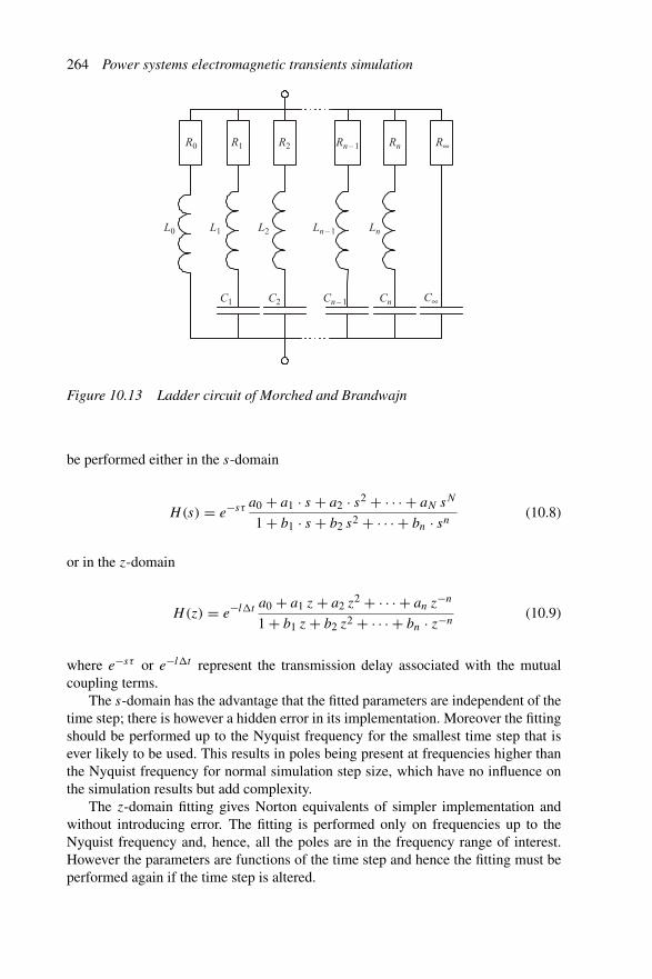
264 Power systems electromagnetic transients simulation
R0 R1 Rn – 1R2 Rn R∞
C∞
L0 L1 Ln – 1L2 Ln
C1 Cn – 1C2 Cn
Figure 10.13 Ladder circuit of Morched and Brandwajn
be performed either in the s-domain
H(s) = e−sτ a0 + a1 · s + a2 · s2 + · · · + aN sN
1 + b1 · s + b2 s2 + · · · + bn · sn(10.8)
or in the z-domain
H(z) = e−l�t a0 + a1 z + a2 z2 + · · · + an z−n
1 + b1 z + b2 z2 + · · · + bn · z−n(10.9)
where e−sτ or e−l�t represent the transmission delay associated with the mutualcoupling terms.
The s-domain has the advantage that the fitted parameters are independent of thetime step; there is however a hidden error in its implementation. Moreover the fittingshould be performed up to the Nyquist frequency for the smallest time step that isever likely to be used. This results in poles being present at frequencies higher thanthe Nyquist frequency for normal simulation step size, which have no influence onthe simulation results but add complexity.
The z-domain fitting gives Norton equivalents of simpler implementation andwithout introducing error. The fitting is performed only on frequencies up to theNyquist frequency and, hence, all the poles are in the frequency range of interest.However the parameters are functions of the time step and hence the fitting must beperformed again if the time step is altered.
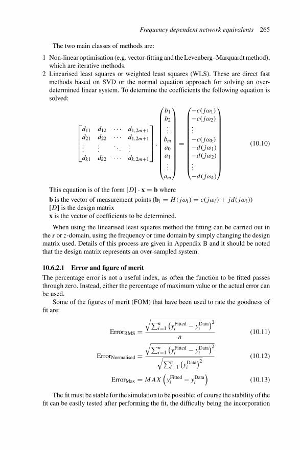
Frequency dependent network equivalents 265
The two main classes of methods are:
1 Non-linear optimisation (e.g. vector-fitting and the Levenberg–Marquardt method),which are iterative methods.
2 Linearised least squares or weighted least squares (WLS). These are direct fastmethods based on SVD or the normal equation approach for solving an over-determined linear system. To determine the coefficients the following equation issolved:
⎡
⎢⎢⎢⎣
d11 d12 · · · d1,2m+1d21 d22 · · · d1,2m+1...
.... . .
...
dk1 dk2 · · · dk,2m+1
⎤
⎥⎥⎥⎦
.
⎛
⎜⎜⎜⎜⎜⎜⎜⎜⎜⎜⎜⎜⎝
b1b2...
bm
a0a1...
am
⎞
⎟⎟⎟⎟⎟⎟⎟⎟⎟⎟⎟⎟⎠
=
⎛
⎜⎜⎜⎜⎜⎜⎜⎜⎜⎜⎜⎜⎝
−c(jω1)
−c(jω2)...
−c(jωk)
−d(jω1)
−d(jω2)...
−d(jωk)
⎞
⎟⎟⎟⎟⎟⎟⎟⎟⎟⎟⎟⎟⎠
(10.10)
This equation is of the form [D] · x = b where
b is the vector of measurement points (bi = H(jωi) = c(jωi) + jd(jωi))[D] is the design matrixx is the vector of coefficients to be determined.
When using the linearised least squares method the fitting can be carried out inthe s or z-domain, using the frequency or time domain by simply changing the designmatrix used. Details of this process are given in Appendix B and it should be notedthat the design matrix represents an over-sampled system.
10.6.2.1 Error and figure of merit
The percentage error is not a useful index, as often the function to be fitted passesthrough zero. Instead, either the percentage of maximum value or the actual error canbe used.
Some of the figures of merit (FOM) that have been used to rate the goodness offit are:
ErrorRMS =√∑n
i=1
(yFittedi − yData
i
)2
n(10.11)
ErrorNormalised =√∑n
i=1
(yFittedi − yData
i
)2
√∑ni=1
(yDatai
)2(10.12)
ErrorMax = MAX(yFittedi − yData
i
)(10.13)
The fit must be stable for the simulation to be possible; of course the stability of thefit can be easily tested after performing the fit, the difficulty being the incorporation
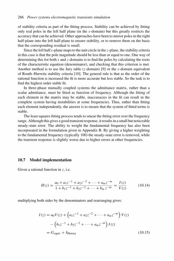
266 Power systems electromagnetic transients simulation
of stability criteria as part of the fitting process. Stability can be achieved by fittingonly real poles in the left half plane (in the s-domain) but this greatly restricts theaccuracy that can be achieved. Other approaches have been to mirror poles in the righthalf-plane into the left half-plane to ensure stability, or to remove them on the basisthat the corresponding residual is small.
Since the left half s-plane maps to the unit circle in the z-plane, the stability criteriain this case is that the pole magnitude should be less than or equal to one. One way ofdetermining this for both s and z-domains is to find the poles by calculating the rootsof the characteristic equation (denominator), and checking that this criterion is met.Another method is to use the Jury table (z-domain) [9] or the s-domain equivalentof Routh–Hurwitz stability criteria [10]. The general rule is that as the order of therational function is increased the fit is more accurate but less stable. So the task is tofind the highest order stable fit.
In three-phase mutually coupled systems the admittance matrix, rather than ascalar admittance, must be fitted as function of frequency. Although the fitting ofeach element in the matrix may be stable, inaccuracies in the fit can result in thecomplete system having instabilities at some frequencies. Thus, rather than fittingeach element independently, the answer is to ensure that the system of fitted terms isstable.
The least squares fitting process tends to smear the fitting error over the frequencyrange. Although this gives a good transient response, it results in a small but noticeablesteady-state error. The ability to weight the fundamental frequency has also beenincorporated in the formulation given in Appendix B. By giving a higher weightingto the fundamental frequency (typically 100) the steady-state error is removed, whilethe transient response is slightly worse due to higher errors at other frequencies.
10.7 Model implementation
Given a rational function in z, i.e.
H(z) = a0 + a1z−1 + a2z
−2 + · · · + amz−m
1 + b1z−1 + b2z−2 + · · · + bm z−m= I (z)
V (z)(10.14)
multiplying both sides by the denominators and rearranging gives:
I (z) = a0V (z) +(a1z
−1 + a2z−2 + · · · + amz−m
)V (z)
−(b1z
−1 + b2z−2 + · · · + amz−m
)I (z)
= Gequiv + IHistory (10.15)
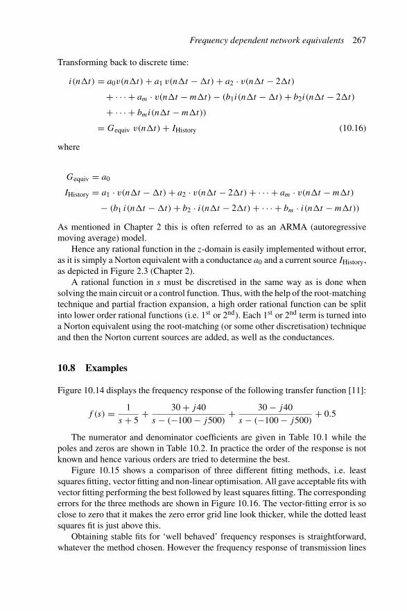
Frequency dependent network equivalents 267
Transforming back to discrete time:
i(n�t) = a0v(n�t) + a1 v(n�t − �t) + a2 · v(n�t − 2�t)
+ · · · + am · v(n�t − m�t) − (b1i(n�t − �t) + b2i(n�t − 2�t)
+ · · · + bmi(n�t − m�t))
= Gequiv v(n�t) + IHistory (10.16)
where
Gequiv = a0
IHistory = a1 · v(n�t − �t) + a2 · v(n�t − 2�t) + · · · + am · v(n�t − m�t)
− (b1 i(n�t − �t) + b2 · i(n�t − 2�t) + · · · + bm · i(n�t − m�t))
As mentioned in Chapter 2 this is often referred to as an ARMA (autoregressivemoving average) model.
Hence any rational function in the z-domain is easily implemented without error,as it is simply a Norton equivalent with a conductance a0 and a current source IHistory,as depicted in Figure 2.3 (Chapter 2).
A rational function in s must be discretised in the same way as is done whensolving the main circuit or a control function. Thus, with the help of the root-matchingtechnique and partial fraction expansion, a high order rational function can be splitinto lower order rational functions (i.e. 1st or 2nd). Each 1st or 2nd term is turned intoa Norton equivalent using the root-matching (or some other discretisation) techniqueand then the Norton current sources are added, as well as the conductances.
10.8 Examples
Figure 10.14 displays the frequency response of the following transfer function [11]:
f (s) = 1
s + 5+ 30 + j40
s − (−100 − j500)+ 30 − j40
s − (−100 − j500)+ 0.5
The numerator and denominator coefficients are given in Table 10.1 while thepoles and zeros are shown in Table 10.2. In practice the order of the response is notknown and hence various orders are tried to determine the best.
Figure 10.15 shows a comparison of three different fitting methods, i.e. leastsquares fitting, vector fitting and non-linear optimisation. All gave acceptable fits withvector fitting performing the best followed by least squares fitting. The correspondingerrors for the three methods are shown in Figure 10.16. The vector-fitting error is soclose to zero that it makes the zero error grid line look thicker, while the dotted leastsquares fit is just above this.
Obtaining stable fits for ‘well behaved’ frequency responses is straightforward,whatever the method chosen. However the frequency response of transmission lines
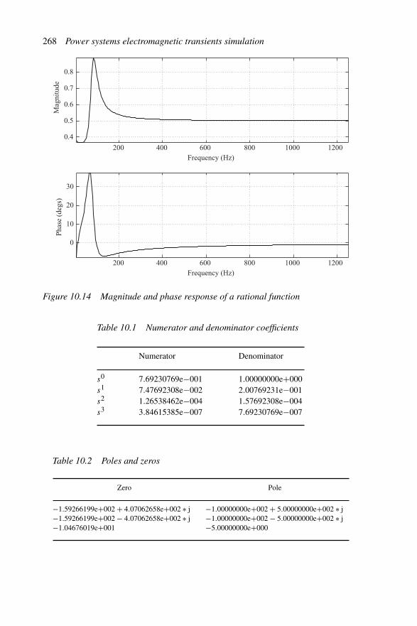
268 Power systems electromagnetic transients simulation
Frequency (Hz)
Mag
nitu
deP
hase
(de
gs)
0.4
0.5
0.6
0.7
0.8
0
10
20
30
200 400 600 800 1000 1200
Frequency (Hz)200 400 600 800 1000 1200
Figure 10.14 Magnitude and phase response of a rational function
Table 10.1 Numerator and denominator coefficients
Numerator Denominator
s0 7.69230769e−001 1.00000000e+000s1 7.47692308e−002 2.00769231e−001s2 1.26538462e−004 1.57692308e−004s3 3.84615385e−007 7.69230769e−007
Table 10.2 Poles and zeros
Zero Pole
−1.59266199e+002 + 4.07062658e+002 ∗ j −1.00000000e+002 + 5.00000000e+002 ∗ j−1.59266199e+002 − 4.07062658e+002 ∗ j −1.00000000e+002 − 5.00000000e+002 ∗ j−1.04676019e+001 −5.00000000e+000

Frequency dependent network equivalents 269
Original frequency responseLeast squares fittingVector fittingNon-linear optimisation
200 400 600 800 1000 1200Frequency (Hz)
Original frequency responseLeast squares fittingVector fittingNon-linear optimisation
0.5
0.6
0.7
0.8
0.4
0
10
20
30
Mag
nitu
de (
ohm
s)P
hase
(de
gs)
200 400 600 800 1000 1200Frequency (Hz)
Figure 10.15 Comparison of methods for the fitting of a rational function
200 400 600 800 1000 1200Frequency (Hz)
200 400 600 800 1000 1200Frequency (Hz)
Rea
l err
or (
%)
Least Squares Fitting
Non- linear optimisation
Imag
err
or (
%)
Least squares fitting Vector fittingNon-linear optimisation
–3.5–3
–2.5–2
–1.5–1
–0.50
–14
–12
–10
–8
–6
–4
–2
0
Vector fitting
Figure 10.16 Error for various fitted methods
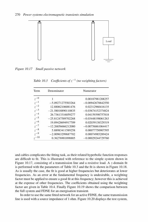
270 Power systems electromagnetic transients simulation
Load
Figure 10.17 Small passive network
Table 10.3 Coefficients of z−1 (no weighting factors)
Term Denominator Numerator
z−0 1 0.00187981208257z−1 −5.09271275503264 −0.00942678842550z−2 12.88062106081476 0.02312960416135z−3 −21.58018890110835 −0.03674152374824z−4 26.73613316059277 0.04159398757818z−5 −25.81247589702268 −0.03448198061263z−6 19.89428694917709 0.02039138329319z−7 −12.26856666212080 −0.00756861064417z−8 5.88983411589258 0.00077750907595z−9 −2.00963299687702 0.00074985289424z−10 0.36276901898885 −0.00029244729760
and cables complicates the fitting task, as their related hyperbolic function responsesare difficult to fit. This is illustrated with reference to the simple system shown inFigure 10.17, consisting of a transmission line and a resistive load. A z-domain fitis performed with the parameters of Table 10.3 and the fit is shown in Figure 10.18.As is usually the case, the fit is good at higher frequencies but deteriorates at lowerfrequencies. As an error at the fundamental frequency is undesirable, a weightingfactor must be applied to ensure a good fit at this frequency; however this is achievedat the expense of other frequencies. The coefficients obtained using the weightingfactor are given in Table 10.4. Finally Figure 10.19 shows the comparison betweenthe full system and FDNE for an energisation transient.
In order to use the same fitted network for an active FDNE, the same transmissionline is used with a source impedance of 1 ohm. Figure 10.20 displays the test system,
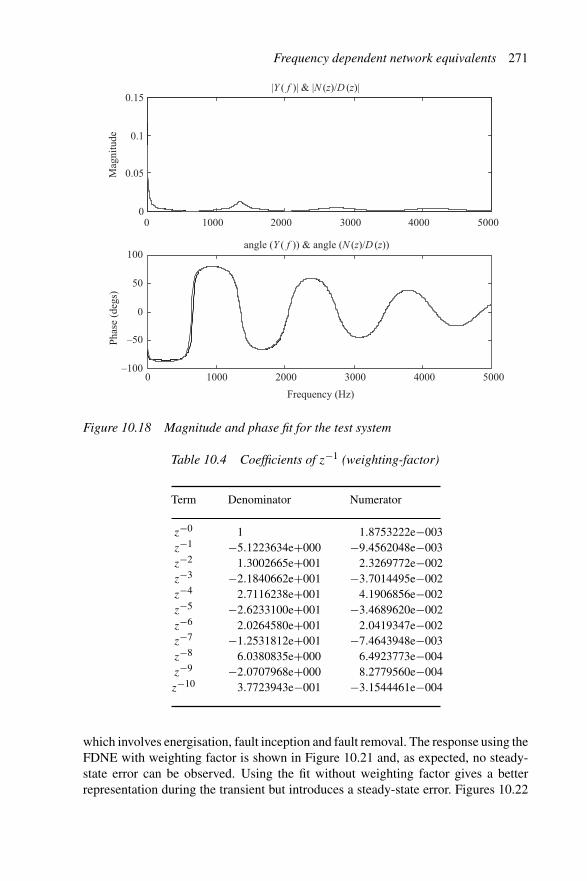
Frequency dependent network equivalents 271
0 1000 2000 3000 4000 5000
|Y ( f )| & |N (z)/D (z)|
Frequency (Hz)
angle (Y ( f )) & angle (N (z)/D (z))
0
0.05
0.1
0.15
–100
–50
0
50
100
Mag
nitu
deP
hase
(de
gs)
0 1000 2000 3000 4000 5000
Figure 10.18 Magnitude and phase fit for the test system
Table 10.4 Coefficients of z−1 (weighting-factor)
Term Denominator Numerator
z−0 1 1.8753222e−003z−1 −5.1223634e+000 −9.4562048e−003z−2 1.3002665e+001 2.3269772e−002z−3 −2.1840662e+001 −3.7014495e−002z−4 2.7116238e+001 4.1906856e−002z−5 −2.6233100e+001 −3.4689620e−002z−6 2.0264580e+001 2.0419347e−002z−7 −1.2531812e+001 −7.4643948e−003z−8 6.0380835e+000 6.4923773e−004z−9 −2.0707968e+000 8.2779560e−004z−10 3.7723943e−001 −3.1544461e−004
which involves energisation, fault inception and fault removal. The response using theFDNE with weighting factor is shown in Figure 10.21 and, as expected, no steady-state error can be observed. Using the fit without weighting factor gives a betterrepresentation during the transient but introduces a steady-state error. Figures 10.22
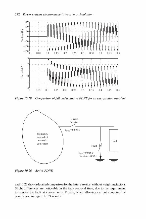
272 Power systems electromagnetic transients simulation
–150
–100
–50
0
50
100
150
0 0.05 0.1 0.15 0.2 0.25 0.3 0.35 0.4 0.45 0.5
–2
–1
0
1
2
3
0 0.05 0.1 0.15 0.2 0.25 0.3 0.35 0.4 0.45 0.5
Vol
tage
(kV
)C
urre
nt (
kA)
Figure 10.19 Comparison of full and a passive FDNE for an energisation transient
Frequencydependentnetwork
equivalentLoad
Fault
Circuitbreaker
tclose = 0.096 s
tfault = 0.025 s Duration = 0.35 s
Figure 10.20 Active FDNE
and 10.23 show a detailed comparison for the latter case (i.e. without weighting factor).Slight differences are noticeable in the fault removal time, due to the requirementto remove the fault at current zero. Finally, when allowing current chopping thecomparison in Figure 10.24 results.
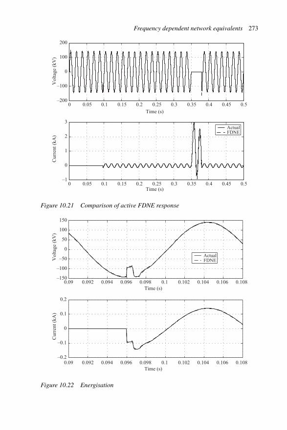
Frequency dependent network equivalents 273
0 0.05 0.1 0.15 0.2 0.25 0.3 0.35 0.4 0.45 0.5Time (s)
0 0.05 0.1 0.15 0.2 0.25 0.3 0.35 0.4 0.45 0.5Time (s)
ActualFDNE
–200
–100
0
100
200
–1
0
1
2
3
Vol
tage
(kV
)C
urre
nt (
kA)
Figure 10.21 Comparison of active FDNE response
Time (s)
ActualFDNE
–150
–100
–50
0
50
100
150
0.09 0.092 0.094 0.096 0.098 0.1 0.102 0.104 0.106 0.108
Time (s)0.09 0.092 0.094 0.096 0.098 0.1 0.102 0.104 0.106 0.108
–0.2
–0.1
0
0.1
0.2
Vol
tage
(kV
)C
urre
nt (
kA)
Figure 10.22 Energisation
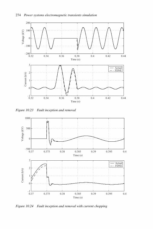
274 Power systems electromagnetic transients simulation
0.32 0.34 0.36 0.38 0.4 0.42 0.44
Vol
tage
(kV
)
Time (s)
0.32 0.34 0.36 0.38 0.4 0.42 0.44Time (s)
Cur
rent
(kA
)
ActualFDNE
–200
–100
0
100
200
–1
0
1
2
3
Figure 10.23 Fault inception and removal
0.37 0.375 0.38 0.385 0.39 0.395 0.4Time (s)
0.37 0.375 0.38 0.385 0.39 0.395 0.4Time (s)
ActualFDNE
–500
0
500
1000
–1
0
1
2
3
Vol
tage
(kV
)C
urre
nt (
kA)
Figure 10.24 Fault inception and removal with current chopping
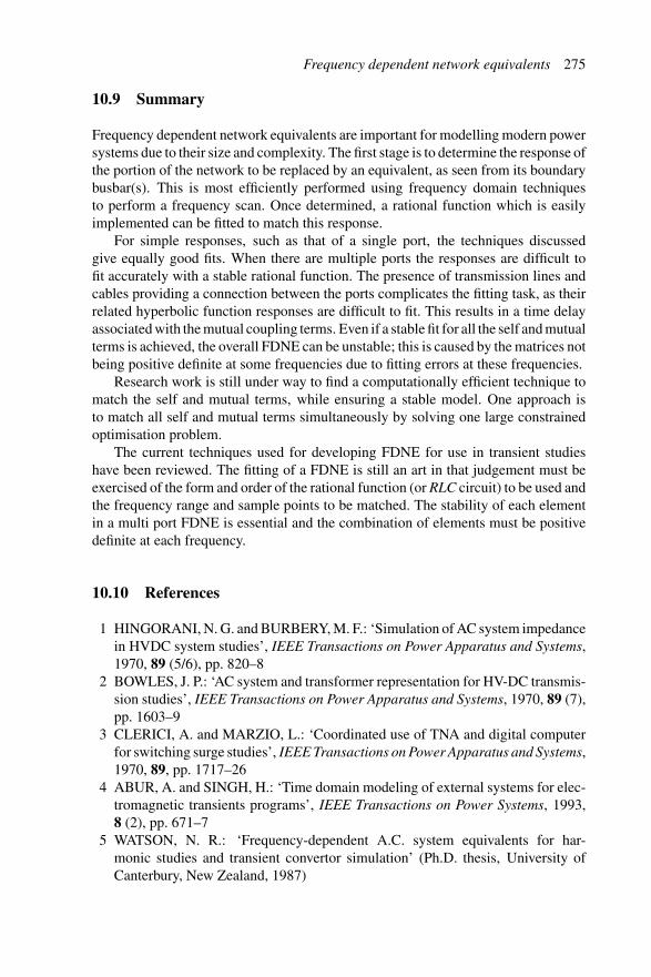
Frequency dependent network equivalents 275
10.9 Summary
Frequency dependent network equivalents are important for modelling modern powersystems due to their size and complexity. The first stage is to determine the response ofthe portion of the network to be replaced by an equivalent, as seen from its boundarybusbar(s). This is most efficiently performed using frequency domain techniquesto perform a frequency scan. Once determined, a rational function which is easilyimplemented can be fitted to match this response.
For simple responses, such as that of a single port, the techniques discussedgive equally good fits. When there are multiple ports the responses are difficult tofit accurately with a stable rational function. The presence of transmission lines andcables providing a connection between the ports complicates the fitting task, as theirrelated hyperbolic function responses are difficult to fit. This results in a time delayassociated with the mutual coupling terms. Even if a stable fit for all the self and mutualterms is achieved, the overall FDNE can be unstable; this is caused by the matrices notbeing positive definite at some frequencies due to fitting errors at these frequencies.
Research work is still under way to find a computationally efficient technique tomatch the self and mutual terms, while ensuring a stable model. One approach isto match all self and mutual terms simultaneously by solving one large constrainedoptimisation problem.
The current techniques used for developing FDNE for use in transient studieshave been reviewed. The fitting of a FDNE is still an art in that judgement must beexercised of the form and order of the rational function (or RLC circuit) to be used andthe frequency range and sample points to be matched. The stability of each elementin a multi port FDNE is essential and the combination of elements must be positivedefinite at each frequency.
10.10 References
1 HINGORANI, N. G. and BURBERY, M. F.: ‘Simulation of AC system impedancein HVDC system studies’, IEEE Transactions on Power Apparatus and Systems,1970, 89 (5/6), pp. 820–8
2 BOWLES, J. P.: ‘AC system and transformer representation for HV-DC transmis-sion studies’, IEEE Transactions on Power Apparatus and Systems, 1970, 89 (7),pp. 1603–9
3 CLERICI, A. and MARZIO, L.: ‘Coordinated use of TNA and digital computerfor switching surge studies’, IEEE Transactions on Power Apparatus and Systems,1970, 89, pp. 1717–26
4 ABUR, A. and SINGH, H.: ‘Time domain modeling of external systems for elec-tromagnetic transients programs’, IEEE Transactions on Power Systems, 1993,8 (2), pp. 671–7
5 WATSON, N. R.: ‘Frequency-dependent A.C. system equivalents for har-monic studies and transient convertor simulation’ (Ph.D. thesis, University ofCanterbury, New Zealand, 1987)
276 Power systems electromagnetic transients simulation
6 MORCHED, A. S. and BRANDWAJN, V.: ‘Transmission network equivalentsfor electromagnetic transient studies’, IEEE Transactions on Power Apparatusand Systems, 1983, 102 (9), pp. 2984–94
7 MORCHED, A. S., OTTEVANGERS, J. H. and MARTI, L.: ‘Multi port fre-quency dependent network equivalents for the EMTP’, IEEE Transactions onPower Delivery, Seattle, Washington, 1993, 8 (3), pp. 1402–12
8 DO, V. Q. and GAVRILOVIC, M. M.: ‘An interactive pole-removal method forsynthesis of power system equivalent networks’, IEEE Transactions on PowerApparatus and Systems, 1984, 103 (8), pp. 2065–70
9 JURY, E. I.: ‘Theory and application of the z-transform method’ (John Wiley,New York, 1964)
10 OGATA, K.: ‘Modern control engineering’ (Prentice Hall International, UpperSaddle River, N. J., 3rd edition, 1997)
11 GUSTAVSEN, B. and SEMLYEN, A.: ‘Rational approximation of frequencydomain response by vector fitting’, IEEE Transaction on Power Delivery, 1999,14 (3), pp. 1052–61
Chapter 11
Steady state applications
11.1 Introduction
Knowledge of the initial conditions is critical to the solution of most power systemtransients. The electromagnetic transient packages usually include some type of fre-quency domain initialisation program [1]–[5] to try and simplify the user’s task.These programs, however, are not part of the electromagnetic transient simulationdiscussed in this book. The starting point in the simulation of a system disturbance isthe steady-state operating condition of the system prior to the disturbance.
The steady-state condition is often derived from a symmetrical (positive sequence)fundamental frequency power-flow program. If this information is read in to initialisethe transient solution, the user must ensure that the model components used in thepower-flow program represent adequately those of the electromagnetic transient pro-gram. In practice, component asymmetries and non-linearities will add imbalanceand distortion to the steady-state waveforms.
Alternatively the steady-state solution can be achieved by the so-called ‘bruteforce’ approach; the simulation is started without performing an initial calculationand is carried out long enough for the transient to settle down to a steady-state condi-tion. Hence the electromagnetic transient programs themselves can be used to derivesteady-state waveforms. It is, thus, an interesting matter to speculate whether the cor-rect approach is to provide an ‘exact’ steady state initialisation for the EMTP methodor to use the latter to derive the final steady-state waveforms. The latter alternative isdiscussed in this chapter with reference to power quality application.
A good introduction to the variety of topics considered under ‘power quality’ canbe found in reference [6] and an in-depth description of the methods currently usedfor its assessment is given in reference [7].
An important part of power quality is steady state (and quasi-steady state)waveform distortion. The resulting information is sometimes presented in the timedomain (e.g. notching) and more often in the frequency domain (e.g. harmonics andinterharmonics).
278 Power systems electromagnetic transients simulation
Although their source of origin is a transient disturbance, i.e. a short-circuit,voltage sags are characterised by their (quasi) steady-state magnitude and duration,which, in general, will display three-phase imbalance; moreover, neither the voltagedrop nor its recovery will take place instantaneously. Thus for specified fault condi-tions and locations the EMTP method provides an ideal tool to determine the voltagesag characteristics.
Randomly varying non-linear loads, such as arc furnaces, as well as substantialand varying harmonic (and interharmonic) content, cause voltage fluctuations thatoften produce flicker. The random nature of the load impedance variation with timeprevents an accurate prediction of the phenomena. However the EMTP method canstill help in the selection of compensating techniques, with arc models based on theexperience of existing installations.
11.2 Initialisation
As already mentioned in the introduction, the electromagnetic transients programrequires auxiliary facilities to initialise the steady-state condition, and only a three-phase harmonic power flow can provide a realistic start. However this is difficult andtime consuming as it involves the preparation of another data set and transfer from oneprogram to another, not to mention the difficulty in ensuring that both are modellingexactly the same system and to the same degree of accuracy.
Often a symmetrical fundamental frequency power-flow program is used due tofamiliarity with and availability of such programs. However failure to consider theimbalance and distortion can cause considerable oscillations, particularly if low fre-quency poorly damped resonant frequencies exist. For this reason PSCAD/EMTDCuses a ‘black-start’ approach whereby sources are ramped from zero up to their finalvalue over a period of time, typically 0.05 s. This often results in reaching steady statequicker than initialising with power-flow results where the distortion and/or imbal-ance is ignored. Synchronous machines have long time constants and therefore specialtechniques are required for an efficient simulation. The rotor is normally locked tothe system frequency and/or the resistance artificially changed to improve dampinguntil the electrical transient has died away, then the rotor is released and the resistancereset to its correct value.
11.3 Harmonic assessment
Although the frequency domain provides accurate information of harmonic distor-tion in linear networks, conventional frequency domain algorithms are inadequate torepresent the system non-linear components.
An early iterative method [8], referred to as IHA (for Iterative Harmonic Analysis),was developed to analyse the harmonic interaction of a.c.–d.c. power systems,whereby the converter response at each iteration was obtained from knowledge ofthe converter terminal voltage waveforms (which could be unbalanced and distorted).
Steady state applications 279
The resulting converter currents were then expressed in terms of harmonic currentinjections to be used in a new iteration of the a.c. system harmonic flow. This method,based on the fixed point iteration (or Gauss) concept, had convergence problemsunder weak a.c. system conditions. An alternative IHA based on Newton’s method [9]provided higher reliability at the expense of greatly increased analytical complexity.
However the solution accuracy achieved with these early methods was very lim-ited due to the oversimplified modelling of the converter (in particular the idealisedrepresentation of the converter switching instants).
An important step in solution accuracy was made with the appearance of theso-called harmonic domain [9], a full Newton solution that took into account the mod-ulating effect of a.c. voltage and d.c. current distortion on the switching instants andconverter control functions. This method performs a linearisation around the operatingpoint that provides sufficient accuracy. In the present state of harmonic domain devel-opment the Jacobian matrix equation combines the system fundamental frequencythree-phase load-flow and the system harmonic balance in the presence of multiplea.c.–d.c. converters. Although in principle any other type of non-linear componentcan be accommodated, the formulation of each new component requires consider-able skill and effort. Accordingly a program for the calculation of the non-sinusoidalperiodic steady state of the system may be of very high dimension and complexity.
11.4 Phase-dependent impedance of non-linear device
Using perturbations the transient programs can help to determine the phase-dependentimpedance of a non-linear device. In the steady state any power system componentcan be represented by a voltage controlled current source: I = F(V ), where I and V
are arrays of frequency phasors. The function F may be non-linear and non-analytic.If F is linear, it may include linear cross-coupling between frequencies, and may benon-analytic, i.e. frequency cross-coupling and phase dependence do not imply non-linearity in the frequency domain. The linearised response of F to a single appliedfrequency may be calculated by:
[�IR
�II
]=
⎡
⎢⎢⎣
∂FR
∂VR
∂FR
∂VI
∂FI
∂VR
∂FI
∂VI
⎤
⎥⎥⎦
[�VR
�VI
](11.1)
where F has been expanded into its component parts. If the Cauchy–Riemann con-ditions hold, then 11.1 can be written in complex form. In the periodic steady state,all passive components (e.g. RLC components) yield partial derivatives which satisfythe Cauchy–Riemann conditions. There is, additionally, no cross-coupling betweenharmonics for passive devices or circuits. With power electronic devices the Cauchy–Riemann conditions will not hold, and there will generally be cross-harmonic couplingas well.
In many cases it is desirable to ignore the phase dependence and obtain a compleximpedance which is as near as possible to the average phase-dependent impedance.
280 Power systems electromagnetic transients simulation
Since the phase-dependent impedance describes a circle in the complex plane asa function of the phase angle of the applied voltage [10], the appropriate phase-independent impedance lies at the centre of the phase-dependent locus. Describingthe phase-dependent impedance as
Z =[z11 z12z21 z22
](11.2)
the phase independent component is given by:
Z =[R −X
X R
](11.3)
where
R = 12 (z11 + z22) (11.4)
X = 12 (z21 − z12) (11.5)
In complex form the impedance is then Z = R + jX.In most cases an accurate analytic description of a power electronic device is
not available, so that the impedance must be obtained by perturbations of a steady-state model. Ideally, the model being perturbed should not be embedded in a largersystem (e.g. a.c. or d.c. systems), and perturbations should be applied to controlinputs as well as electrical terminals. The outcome from such an exhaustive studywould be a harmonically cross-coupled admittance tensor completely describing thelinearisation.
The simplest method for obtaining the impedance by perturbation is to sequentiallyapply perturbations in the system source, one frequency at a time, and calculateimpedances from
Zk = �Vk
�Ik
(11.6)
The Zk obtained by this method includes the effect of coupling to the sourceimpedance at frequencies coupled to k by the device, and the effect of phase depen-dency. This last means that for some k, Zk will be located at some unknown positionon the circumference of the phase-dependent impedance locus. The impedance at fre-quencies close to k will lie close to the centre of this locus, which can be obtained byapplying two perturbations in quadrature. With the two perturbations of the quadra-ture method, enough information is available to resolve the impedance into twocomponents; phase dependent and phase independent.
The quadrature method proceeds by first solving a base case at the frequencyof interest to obtain the terminal voltage and total current: (Vkb, Ikb). Next, twoperturbations are applied sequentially to obtain (Vk1, Ik1) and (Vk2, Ik2). If the sourcewas initially something like
Eb = E sin (ωt) (11.7)
Steady state applications 281
then the two perturbations might be
E1 = E sin (ωt) + δ sin (kωt) (11.8)
E2 = E sin (ωt) + δ sin (kωt + π/2) (11.9)
where δ is small to avoid exciting any non-linearity. The impedance is obtained byfirst forming the differences in terminal voltage and injected current:
�Vk1 = Vk1 − Vkb (11.10)
�Vk2 = Vk2 − Vkb (11.11)
�Ik1 = Ik1 − Ikb (11.12)
�Ik2 = Ik2 − Ikb (11.13)
Taking real components, the linear model to be fitted states that[�Vk1R
�Vk1I
]=
[zk11 zk12zk21 zk22
] [�Ik1R
�Ik1I
](11.14)
and [�Vk2R
�Vk2I
]=
[zk11 zk12zk21 zk22
] [�Ik2R
�Ik2I
](11.15)
which permits a solution for the components zk11, etc:⎡
⎢⎢⎣
�Vk1R
�Vk1I
�Vk2R
�Vk2I
⎤
⎥⎥⎦ =
⎡
⎢⎢⎣
�Ik1R �Ik1I 0 00 0 �Ik1R �Ik1I
�Ik2R �Ik2I 0 00 0 �Ik2R �Ik2I
⎤
⎥⎥⎦
⎡
⎢⎢⎣
zk11zk12zk21zk22
⎤
⎥⎥⎦ (11.16)
Finally the phase-independent impedance in complex form is:
Zk = 12 (zk11 + zk22) + 1
2j (zk21 − zk12) (11.17)
11.5 The time domain in an ancillary capacity
The next two sections review the increasing use of the time domain to try and finda simpler alternative to the harmonic solution. In this respect the flexibility of theEMTP method to represent complex non-linearities and control systems makes it anattractive alternative for the solution of harmonic problems. Two different modellingphilosophies have been proposed. One, discussed in this section, is basically a fre-quency domain solution with periodic excursions into the time domain to update thecontribution of the non-linear components. The alternative, discussed in section 11.6,is basically a time domain solution to the steady state followed by FFT processing ofthe resulting waveforms.
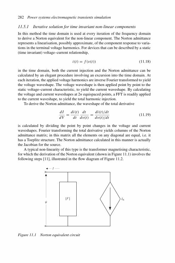
282 Power systems electromagnetic transients simulation
11.5.1 Iterative solution for time invariant non-linear components
In this method the time domain is used at every iteration of the frequency domainto derive a Norton equivalent for the non-linear component. The Norton admittancerepresents a linearisation, possibly approximate, of the component response to varia-tions in the terminal voltage harmonics. For devices that can be described by a static(time invariant) voltage–current relationship,
i(t) = f (v(t)) (11.18)
in the time domain, both the current injection and the Norton admittance can becalculated by an elegant procedure involving an excursion into the time domain. Ateach iteration, the applied voltage harmonics are inverse Fourier transformed to yieldthe voltage waveshape. The voltage waveshape is then applied point by point to thestatic voltage–current characteristic, to yield the current waveshape. By calculatingthe voltage and current waveshapes at 2n equispaced points, a FFT is readily appliedto the current waveshape, to yield the total harmonic injection.
To derive the Norton admittance, the waveshape of the total derivative
dI
dV= di(t)
dt
dt
dv(t)= di(t)/dt
dv(t)/dt(11.19)
is calculated by dividing the point by point changes in the voltage and currentwaveshapes. Fourier transforming the total derivative yields columns of the Nortonadmittance matrix; in this matrix all the elements on any diagonal are equal, i.e. ithas a Toeplitz structure. The Norton admittance calculated in this manner is actuallythe Jacobian for the source.
A typical non-linearity of this type is the transformer magnetising characteristic,for which the derivation of the Norton equivalent (shown in Figure 11.1) involves thefollowing steps [11], illustrated in the flow diagram of Figure 11.2.
I
[F ] IN
Figure 11.1 Norton equivalent circuit

Steady state applications 283
i
i
t
t
1
2
3
4
5
6
Power-flow
No
Yes
( )( )
→ Vb
V j +1 = V j +1 –V j
→ IN = Ib –[H ]Vb
→ c�, c �, [H ]
→ i�, i�, Ib
ik + 1 – ik – 1
k + 1 – k – 1→ f � =
Using nodal or equivalent approach combine the linear and the linearised models and solve for the new state
Convergencereached?
End
FFT of magnetising current
Time derivative of I = f () evaluated
FFT applied to derivative
Harmonic admittance matrix and Norton equivalent current evaluated
Figure 11.2 Description of the iterative algorithm
284 Power systems electromagnetic transients simulation
1 For each phase the voltage waveform is used to derive the corresponding flux waveand the latter is impressed, point by point, upon the experimental characteristicφ–I and the associated magnetising current is then determined in the time domain.
2 By means of an FFT the magnetising current is solved in the frequency domainand the Fourier coefficients i′ and i′′ are assembled into a base current vector Ib.
3 Using the magnetising current and flux as determined in step 1, the time derivativeof the function I = f (φ) is evaluated.
4 The FFT is applied to the slope shape of step 3, and the Fourier coefficients c′ andc′′ obtained from this exercise are used to assemble the Toeplitz matrix [H ].
5 The Norton equivalent current source IN , i.e. IN = Ib − [H ]Vb is calculated.6 The above linearised model is combined with the linear network as part of a Newton-
type iterative solution as described in Figure 11.2, with the Jacobian defined by thematrix [H ].
11.5.2 Iterative solution for general non-linear components
Time-variant non-linear components, such as power electronic devices, do not fall intothe category defined by equation 11.18. Instead their voltage–current relationshipsresult from many interdependent factors, such as the phase and magnitude of each ofthe a.c. voltage and current harmonic components, control system functions, firingangle constraints, etc.
In these cases the converter Norton admittance matrix does not display the Toeplitzcharacteristic, and, in general, contains of the order of n2 different elements, asopposed to the n elements obtained from the FFT. Thus, not only is the calculation ofa harmonic Norton equivalent computationally difficult but, for accurate results, it hasto be iteratively updated. The computational burden is thus further increased in directproportion with the size of the system and the number of harmonics represented.
To extend the iterative algorithm to any type of non-linearity, a generally applica-ble time domain solution (such as the state variable or the EMTP methods) must beused to represent the behaviour of the non-linear components [12], [13].
As in the previous case, the system is divided into linear and non-linear parts.Again, the inputs to a component are the voltages at its terminal and the output, theterminal currents, and both of these will, in general, contain harmonics. The iterativesolution proceeds in two stages.
In the first stage the periodic steady state of the individual components is ini-tially derived from a load-flow program and then updated using voltage correctionsfrom the second stage. The calculations are performed in the frequency domainwhere appropriate (e.g. in the case of transmission lines) and in the time domainotherwise.
The currents obtained in stage (i) are used in stage (ii) to derive the currentmismatches �i, expressed in the frequency domain. These become injections into asystem-wide incremental harmonic admittance matrix Y, calculated in advance fromsuch matrices for all the individual components. The equation �i = Y�v is thensolved for �v to be used in stage (i) to update all bus voltages.
Steady state applications 285
The first stage uses a modular approach, but in the second stage the voltagecorrections are calculated globally, for the whole system. However, convergence isonly achieved linearly, because of the approximations made on the accuracy of v.A separate iterative procedure is needed to model the controllers of active non-lineardevices, such as a.c.–d.c. converters, and this procedure relies entirely on informationfrom the previous iteration.
11.5.3 Acceleration techniques
Time domain simulation, whether performed by the EMTP, state variable or any othermethod, may require large computation times to reach steady state and thus the useof accelerating techniques [14], [15] is advocated to speed up the solution. Thesetechniques take advantage of the two-point boundary value inherent in the steady-state condition. Thus a correction term is added to the initial state vector, calculatedas a function of the residuum of the initial and final state vectors and the mappingderivative over the period. A concise version of the Poincaré method described inreference [14] is given here.
A non-linear system of state equations is expressed as:
x = g(x, u) x(t0) = x0 (11.20)
where u = u(t) is the input and x0 the vector of state variables at t = t0 close to theperiodic steady state.
This state is characterised by the condition
f (x0) = x(t0 + T ) − x(t0) (11.21)
where x(t0 + T ) is derived by numerical integration over the period t0 to t0 + T ofthe state equations 11.20
Equation 11.21 represents a system of n non-linear algebraic equations withn unknown xi and can thus be solved by the Newton–Raphson method.
The linearised form of equation 11.21 around an approximation x(k)0 at step k of
its solution is:
f (x0) ∼= f(
x(k)0
)+ J (k)
(x(k+1)
0 − x(k)0
)= 0 (11.22)
where J (k) is the Jacobian (the matrix of partial derivatives of f (x0) with respect to x,evaluated at x(k)
0 ). By approximating J (k) at each iteration k, using its definition, inaddition to the mapping
x(k)0 → f
(x(k)
0
)(11.23)
the mappings are
x(k)0 + εIi → f
(x
(k)0 + εIi
)i = 1, . . . , n (11.24)

286 Power systems electromagnetic transients simulation
where Ii are the columns of the unit matrix and ε is a small scalar. J (k) is thenassembled from the vectors
1
ε
(f(
x(k)0 + εIi
)+ f
(x(k)
0
))i = 1, . . . , n (11.25)
obtained in equations 11.23 and 11.24.Finally, using the above approximation J (k) of the Jacobian, the updated value
x(k+1)0 for x0 is obtained from equation 11.22.
The process described above is quasi-Newton but its convergence is close toquadratic. Therefore, as in a conventional Newton power-flow program, only threeto five iterations are needed for convergence to a highly accurate solution, dependingon the closeness of the initial state x0 to the converged solution.
11.6 The time domain in the primary role
11.6.1 Basic time domain algorithm
Starting from standstill, the basic time domain uses a ‘brute force’ solution, i.e. thesystem equations are integrated until a reasonable steady state is reached. This isa very simple approach but can have very slow convergence when the network hascomponents with light damping.
To alleviate this problem the use of acceleration techniques has been describedin sections 11.5.2 and 11.5.3 with reference to the hybrid solution. However thenumber of periods to be processed in the time domain required by the accelerationtechnique is almost directly proportional to the number of state variables multipliedby the number of Newton iterations [14]. Therefore the solution efficiency reducesvery rapidly as the a.c. system size increases. This is not a problem in the case of thehybrid algorithm, because the time domain solutions require no explicit representationof the a.c. network. On the other hand, when the solution is carried out entirely in thetime domain, the a.c. system components are included in the formulation and thusthe number of state variables is always large. Moreover, the time domain algorithmonly requires a single transient simulation to steady state, and therefore the advantageof the acceleration technique is questionable in this case, considering its additionalcomplexity.
On reaching the steady state within a specified tolerance, the voltage and currentwaveforms, represented by sets of discrete values at equally spaced intervals (corre-sponding with the integration steps), are subjected to FFT processing to derive theharmonic spectra.
11.6.2 Time step
The time step selection is critical to model accurately the resonant conditions whenconverters are involved. A resonant system modelled with 100 or 50 μs steps canmiss a resonance, while the use of a 10 μs captures it. Moreover, the higher theresonant frequency the smaller the step should be. A possible way of checking the
Steady state applications 287
effectiveness of a given time step is to reduce the step and then compare the resultswith those obtained in the previous run. If there is a significant change around theresonant frequency, then the time step is too large.
The main reason for the small time-step requirement is the need to pin-pointthe commutation instants very accurately, as these have great influence on the pos-itive feedback that appears to occur between the a.c. harmonic voltages and thecorresponding driven converter currents.
11.6.3 DC system representation
It is essential to represent correctly the main components of the particular converterconfiguration. For instance, a voltage source converter should include the d.c. capac-itor explicitly, while a current source converter should instead include the seriesinductor.
The inverter end representation, although less critical, may still have some effect.An ideal d.c. current source or a series R–L load representation are the simplestsolutions; in the latter case the R is based on the d.c. load-flow operating pointand the inductance should be roughly twice the inverter a.c. inductance (includingtransformer leakage plus any a.c. system inductance). A pure resistance is not advisedas this will produce an overdamped d.c. system, which may lead to inaccurate results.
11.6.4 AC system representation
The main advantage claimed by the hybrid frequency/time domain methods, describedin section 11.5, over conventional time domain solutions is their ability to modelaccurately the frequency dependence of the a.c. system components (particularlythe transmission lines). Thus, if the time domain is going to be favoured in futureharmonic simulations, the accuracy of its frequency dependent components needs tobe greatly improved.
The use of a frequency dependent equivalent avoids the need to model any sig-nificant part of the a.c. system in detail, yet can still provide an accurate matching ofthe system impedance across the harmonic frequency spectra [16]. The derivation offrequency dependent equivalents is described in Chapter 10.
On completion of the time domain simulation, the FFT-derived harmonic currentspectrum at the converter terminals needs to be injected into the full a.c. system todetermine the harmonic flows throughout the actual system components.
By way of example, the test system of Figure 11.3 includes part of the pri-mary transmission system connected to the rectifier end of the New Zealand HVDClink [17]. Though not shown in the diagram, the converter terminal also contains aset of filters as per the CIGRE benchmark model [18].
The corresponding frequency dependent equivalent circuit is shown in Figure 11.4and its component values in Table 11.1. A graph of the impedance magnitude ofthe actual rectifier a.c. system based on its modelled parameters, and the frequencydependent equivalent, is given in Figure 11.5. It can be seen that this equivalentprovides a very good match for the impedance of the actual system up to about the
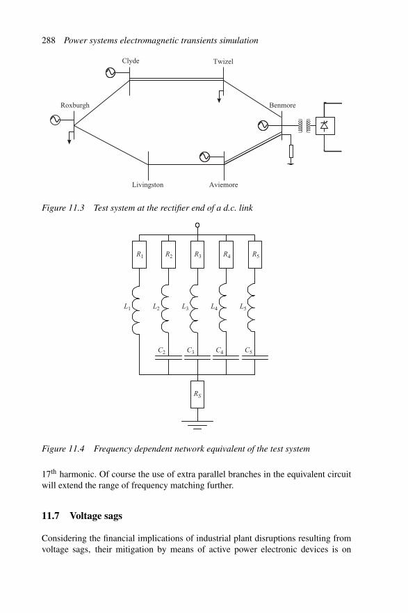
288 Power systems electromagnetic transients simulation
Clyde
Roxburgh
Livingston Aviemore
Benmore
Twizel
Figure 11.3 Test system at the rectifier end of a d.c. link
R1 R2 R3 R4 R5
L1 L2 L3 L4 L5
C2 C3 C4 C5
RS
Figure 11.4 Frequency dependent network equivalent of the test system
17th harmonic. Of course the use of extra parallel branches in the equivalent circuitwill extend the range of frequency matching further.
11.7 Voltage sags
Considering the financial implications of industrial plant disruptions resulting fromvoltage sags, their mitigation by means of active power electronic devices is on
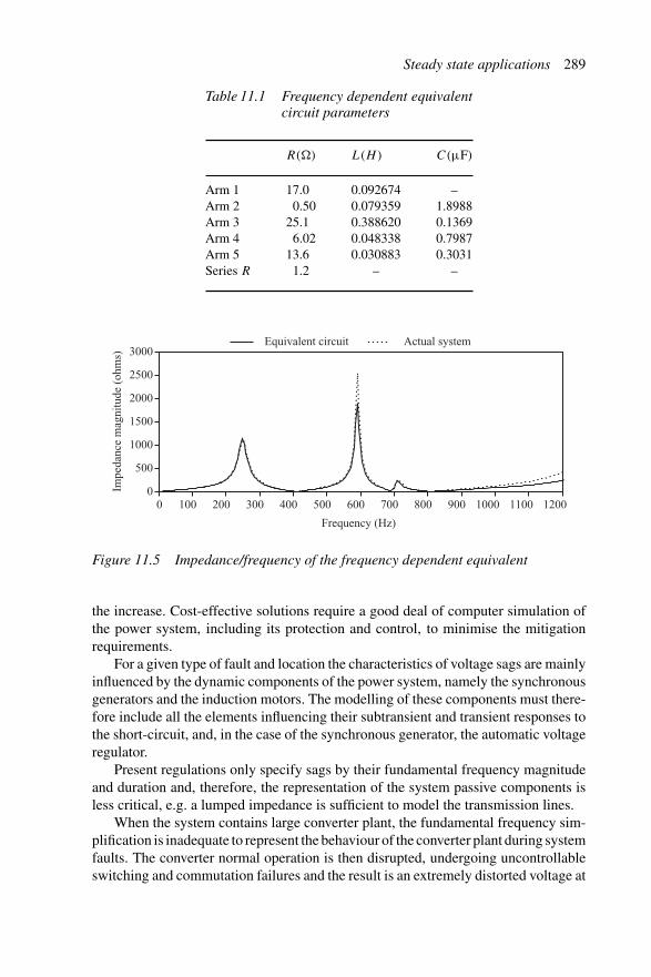
Steady state applications 289
Table 11.1 Frequency dependent equivalentcircuit parameters
R(�) L(H) C(μF)
Arm 1 17.0 0.092674 –Arm 2 0.50 0.079359 1.8988Arm 3 25.1 0.388620 0.1369Arm 4 6.02 0.048338 0.7987Arm 5 13.6 0.030883 0.3031Series R 1.2 – –
Impe
danc
e m
agni
tude
(oh
ms)
0 100 200 300 400 500 600 700 800 900 1000 1100 1200
Frequency (Hz)
Equivalent circuit Actual system
0
500
1000
1500
2000
2500
3000
Figure 11.5 Impedance/frequency of the frequency dependent equivalent
the increase. Cost-effective solutions require a good deal of computer simulation ofthe power system, including its protection and control, to minimise the mitigationrequirements.
For a given type of fault and location the characteristics of voltage sags are mainlyinfluenced by the dynamic components of the power system, namely the synchronousgenerators and the induction motors. The modelling of these components must there-fore include all the elements influencing their subtransient and transient responses tothe short-circuit, and, in the case of the synchronous generator, the automatic voltageregulator.
Present regulations only specify sags by their fundamental frequency magnitudeand duration and, therefore, the representation of the system passive components isless critical, e.g. a lumped impedance is sufficient to model the transmission lines.
When the system contains large converter plant, the fundamental frequency sim-plification is inadequate to represent the behaviour of the converter plant during systemfaults. The converter normal operation is then disrupted, undergoing uncontrollableswitching and commutation failures and the result is an extremely distorted voltage at
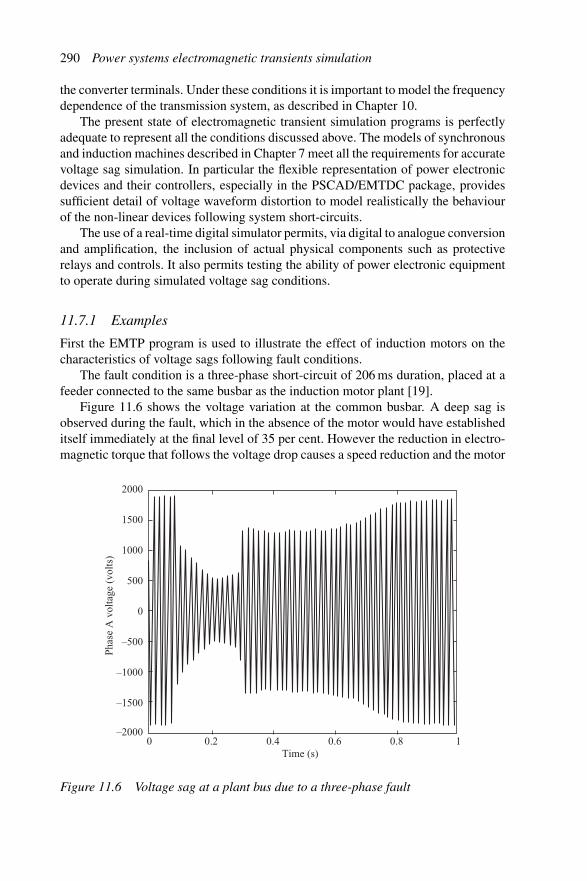
290 Power systems electromagnetic transients simulation
the converter terminals. Under these conditions it is important to model the frequencydependence of the transmission system, as described in Chapter 10.
The present state of electromagnetic transient simulation programs is perfectlyadequate to represent all the conditions discussed above. The models of synchronousand induction machines described in Chapter 7 meet all the requirements for accuratevoltage sag simulation. In particular the flexible representation of power electronicdevices and their controllers, especially in the PSCAD/EMTDC package, providessufficient detail of voltage waveform distortion to model realistically the behaviourof the non-linear devices following system short-circuits.
The use of a real-time digital simulator permits, via digital to analogue conversionand amplification, the inclusion of actual physical components such as protectiverelays and controls. It also permits testing the ability of power electronic equipmentto operate during simulated voltage sag conditions.
11.7.1 Examples
First the EMTP program is used to illustrate the effect of induction motors on thecharacteristics of voltage sags following fault conditions.
The fault condition is a three-phase short-circuit of 206 ms duration, placed at afeeder connected to the same busbar as the induction motor plant [19].
Figure 11.6 shows the voltage variation at the common busbar. A deep sag isobserved during the fault, which in the absence of the motor would have establisheditself immediately at the final level of 35 per cent. However the reduction in electro-magnetic torque that follows the voltage drop causes a speed reduction and the motor
Pha
se A
vol
tage
(vo
lts)
0 0.2 0.4 0.6 0.8 1Time (s)
2000
1500
1000
500
0
–500
–1000
–1500
–2000
Figure 11.6 Voltage sag at a plant bus due to a three-phase fault
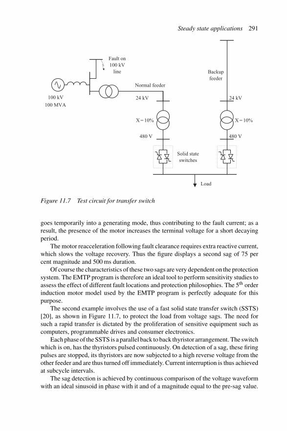
Steady state applications 291
Solid state switches
Load
Normal feeder
Backupfeeder
100 kV
100 MVA
Fault on 100 kV
line
24 kV 24 kV
480 V480 V
X = 10% X = 10%
Figure 11.7 Test circuit for transfer switch
goes temporarily into a generating mode, thus contributing to the fault current; as aresult, the presence of the motor increases the terminal voltage for a short decayingperiod.
The motor reacceleration following fault clearance requires extra reactive current,which slows the voltage recovery. Thus the figure displays a second sag of 75 percent magnitude and 500 ms duration.
Of course the characteristics of these two sags are very dependent on the protectionsystem. The EMTP program is therefore an ideal tool to perform sensitivity studies toassess the effect of different fault locations and protection philosophies. The 5th orderinduction motor model used by the EMTP program is perfectly adequate for thispurpose.
The second example involves the use of a fast solid state transfer switch (SSTS)[20], as shown in Figure 11.7, to protect the load from voltage sags. The need forsuch a rapid transfer is dictated by the proliferation of sensitive equipment such ascomputers, programmable drives and consumer electronics.
Each phase of the SSTS is a parallel back to back thyristor arrangement. The switchwhich is on, has the thyristors pulsed continuously. On detection of a sag, these firingpulses are stopped, its thyristors are now subjected to a high reverse voltage from theother feeder and are thus turned off immediately. Current interruption is thus achievedat subcycle intervals.
The sag detection is achieved by continuous comparison of the voltage waveformwith an ideal sinusoid in phase with it and of a magnitude equal to the pre-sag value.

292 Power systems electromagnetic transients simulation
kV0.4
0.2
0
–0.2
–0.40.18 0.19 0.2 0.21 0.22 0.23 0.24 0.25
s
cust_vol_transferred cust_vol
Figure 11.8 Transfer for a 30 per cent sag at 0.8 power factor with a 3325 kVA load
The latter is constructed using the fundamental frequency component of the FFT ofthe voltage waveform from the previous cycle.
The voltage waveforms derived from PSCAD/EMTDC simulation, following adisturbance in the circuit of Figure 11.7, are shown in Figure 11.8. The continuoustrace shows that the feeder transfer is achieved within quarter of a cycle and withminimal transients. The dotted line shows the voltage that would have appeared atthe load in the absence of a transfer switch.
11.8 Voltage fluctuations
Low frequency voltage fluctuations give rise to the flicker effect, defined as the varia-tion in electric lamp luminosity which affects human vision. The problem frequenciescausing flicker are in the region of 0.5–25 Hz, the most critical value being 8.3 Hz,for which even a 0.3 per cent voltage amplitude variation can reach the perceptibilitythreshold.
The main cause of voltage fluctuation is the electric arc furnace (EAF), due tothe continuous non-linear variation of the arc resistance, particularly during the melt-ing cycle. A physical analysis of the arc length variation is impractical due to thevarying metal scrap shapes, the erratic electromagnetic forces and the arc-electrodepositions. Instead, the EAF is normally represented by simplified deterministic or sto-chastic models, with the purpose of determining the effect of possible compensationtechniques.
By way of example, Figure 11.9 shows a single line diagram of an 80 MVA arcfurnace system fed from a 138 kV bus with a 2500 MVA short-circuit capacity [21].The EAF transformer secondary voltage is 15 kV and the EAF operates at 900 V. TheEAF behaviour is simulated in the PSCAD/EMTDC program by a chaotic arc modeland the power delivered to the EAF is kept constant at 80 MVA by adjusting the tapchangers on the EAF transformers.
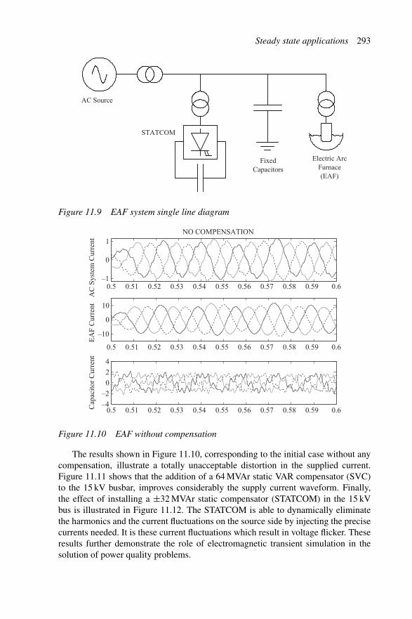
Steady state applications 293
FixedCapacitors
STATCOM
AC Source
Electric ArcFurnace(EAF)
Figure 11.9 EAF system single line diagram
–1
0
1NO COMPENSATION
–10
0
10
–4
–2
0
2
4
0.5 0.51 0.52 0.53 0.54 0.55 0.56 0.57 0.58 0.59 0.6
0.5 0.51 0.52 0.53 0.54 0.55 0.56 0.57 0.58 0.59 0.6
0.5 0.51 0.52 0.53 0.54 0.55 0.56 0.57 0.58 0.59 0.6
AC
Sys
tem
Cur
rent
EA
F C
urre
ntC
apac
itor
Cur
rent
Figure 11.10 EAF without compensation
The results shown in Figure 11.10, corresponding to the initial case without anycompensation, illustrate a totally unacceptable distortion in the supplied current.Figure 11.11 shows that the addition of a 64 MVAr static VAR compensator (SVC)to the 15 kV busbar, improves considerably the supply current waveform. Finally,the effect of installing a ±32 MVAr static compensator (STATCOM) in the 15 kVbus is illustrated in Figure 11.12. The STATCOM is able to dynamically eliminatethe harmonics and the current fluctuations on the source side by injecting the precisecurrents needed. It is these current fluctuations which result in voltage flicker. Theseresults further demonstrate the role of electromagnetic transient simulation in thesolution of power quality problems.
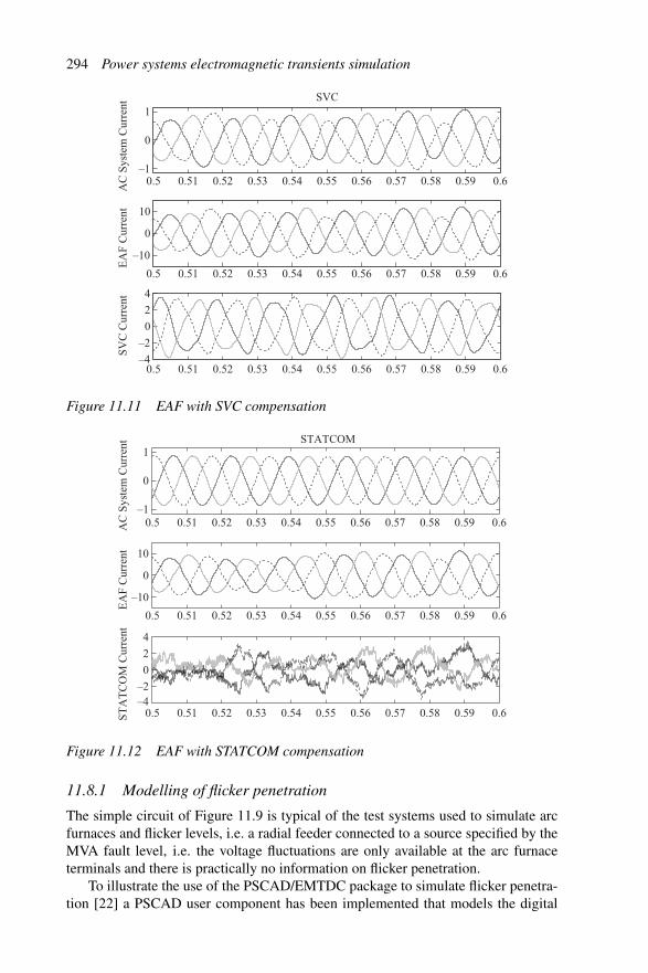
294 Power systems electromagnetic transients simulation
–1
0
1SVC
–10
0
10
–4
–2
0
2
4
0.5 0.51 0.52 0.53 0.54 0.55 0.56 0.57 0.58 0.59 0.6
0.5 0.51 0.52 0.53 0.54 0.55 0.56 0.57 0.58 0.59 0.6
0.5 0.51 0.52 0.53 0.54 0.55 0.56 0.57 0.58 0.59 0.6
AC
Sys
tem
Cur
rent
EA
F C
urre
ntS
VC
Cur
rent
Figure 11.11 EAF with SVC compensation
STATCOM
0.5 0.51 0.52 0.53 0.54 0.55 0.56 0.57 0.58 0.59 0.6
0.5 0.51 0.52 0.53 0.54 0.55 0.56 0.57 0.58 0.59 0.6
0.5 0.51 0.52 0.53 0.54 0.55 0.56 0.57 0.58 0.59 0.6
AC
Sys
tem
Cur
rent
EA
F C
urre
ntS
TA
TC
OM
Cur
rent
–1
0
1
–10
0
10
–4–2
0
2
4
Figure 11.12 EAF with STATCOM compensation
11.8.1 Modelling of flicker penetration
The simple circuit of Figure 11.9 is typical of the test systems used to simulate arcfurnaces and flicker levels, i.e. a radial feeder connected to a source specified by theMVA fault level, i.e. the voltage fluctuations are only available at the arc furnaceterminals and there is practically no information on flicker penetration.
To illustrate the use of the PSCAD/EMTDC package to simulate flicker penetra-tion [22] a PSCAD user component has been implemented that models the digital

Steady state applications 295
4
2
6 5
1
3
4 52
3
1
Tiwai 220
Manapouri 220 Roxburgh 220
Roxb 11Invc 33
current injection
Invercargill 220
Figure 11.13 Test system for flicker penetration (the circles indicate busbars andthe squares transmission lines)
version of the IEC flickermeter. The unit receives the input signal from the timedomain simulation and produces the instantaneous flicker level (IFL) as well as theshort-term and long-term flicker severity indices (Pst,Plt). Moreover, a number ofthese components are needed to study the propagation of flicker levels throughout thepower system.
However, the observation time for the Pst index is 10 minutes, resulting in verylong runs. For example to complete ten minutes of simulation of the nine-bus systemshown in Figure 11.13 requires about twelve hours of running time in an UltraSPARCcomputer (300 MHz). In Figure 11.13 the flicker injection, at the Tiwai busbar,consists of three sinusoidally amplitude modulated current sources that operate at50 ± f Hz.
The voltages at the load and transmission system buses are monitored by 18 iden-tical flicker meters. To reduce the simulation burden the observation time for thePst evaluation was set to 10 seconds instead of 10 minutes. A control block allowsstepping automatically through the list of specified frequencies (1–35 Hz) during thesimulation run and also to selectively record the output channels.
Figure 11.14 is an example of the flicker severities monitored at the various pointsprovided with the virtual flicker meters used with the EMTDC program. For com-parison the figure also includes the flicker levels derived from steady-state frequencydomain analysis. The flicker severity is highest at the Tiwai bus, which has to beexpected since it is the point of injection. Comparing Figures 11.14(b) and (e) andFigures 11.14(d) and (f) respectively it can be seen that, for a positive sequenceinjection, flicker propagates almost without attenuation from the transmission to theload busbars.
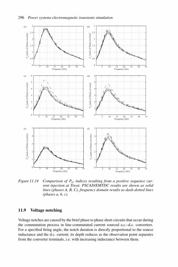
296 Power systems electromagnetic transients simulation
AA
B
B
C
C
a
a
b
b
c
c
AA
B
B
C
C
a
a
b
b
c
c
Frequency [Hz]
Pst [
unit
s of
fli
cker
sev
erit
y]
0
0.5
1
1.5
2
2.5
3
5 10 15 20 25 30 35
Frequency [Hz]
Pst [
unit
s of
fli
cker
sev
erit
y]P
st [
unit
s of
fli
cker
sev
erit
y]
0
1
2
3
4
5
6
5 10 15 20 25 30 35Frequency [Hz]
Pst [
unit
s of
fli
cker
sev
erit
y]
0
1
2
3
4
5
6
5 10 15 20 25 30 35
Frequency [Hz]
Pst [
unit
s of
fli
cker
sev
erit
y]
0
0.5
1
1.5
2
2.5
3
5 10 15 20 25 30 35
AA
B
B
C
C
a
a
b
b
c
c
AA
B
B
C
C
a
a
b
b
c
c
5 10 15 20 25 30 35
AA
B
B
C
C
a
a
b
b
c
c
Frequency [Hz]
0
1
2
3
4
5
Pst [
unit
s of
fli
cker
sev
erit
y]
5 10 15 20 25 30 35Frequency [Hz]
0
1
2
3
4
5
AA
B
B
C
C
a
a
b
b
c
c
(a) (b)
(c) (d)
(e) (f)
Figure 11.14 Comparison of Pst indices resulting from a positive sequence cur-rent injection at Tiwai. PSCAD/EMTDC results are shown as solidlines (phases A, B, C), frequency domain results as dash-dotted lines(phases a, b, c).
11.9 Voltage notching
Voltage notches are caused by the brief phase to phase short-circuits that occur duringthe commutation process in line-commutated current sourced a.c.–d.c. converters.For a specified firing angle, the notch duration is directly proportional to the sourceinductance and the d.c. current; its depth reduces as the observation point separatesfrom the converter terminals, i.e. with increasing inductance between them.
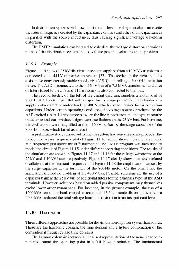
Steady state applications 297
In distribution systems with low short-circuit levels, voltage notches can excitethe natural frequency created by the capacitance of lines and other shunt capacitancesin parallel with the source inductance, thus causing significant voltage waveformdistortion.
The EMTP simulation can be used to calculate the voltage distortion at variouspoints of the distribution system and to evaluate possible solutions to the problem.
11.9.1 Example
Figure 11.15 shows a 25 kV distribution system supplied from a 10 MVA transformerconnected to a 144 kV transmission system [23]. The feeder on the right includesa six-pulse converter adjustable speed drive (ASD) controlling a 6000 HP inductionmotor. The ASD is connected to the 4.16 kV bus of a 7.5 MVA transformer and a setof filters tuned to the 5, 7 and 11 harmonics is also connected to that bus.
The second feeder, on the left of the circuit diagram, supplies a motor load of800 HP at 4.16 kV in parallel with a capacitor for surge protection. This feeder alsosupplies other smaller motor loads at 480 V which include power factor correctioncapacitors. Under certain operating conditions the voltage notches produced by theASD excited a parallel resonance between the line capacitance and the system sourceinductance and thus produced significant oscillations on the 25 kV bus. Furthermore,the oscillations were magnified at the 4.16 kV busbar by the surge capacitor of the800 HP motor, which failed as a result.
A preliminary study carried out to find the system frequency response produced theimpedance versus frequency plot of Figure 11.16, which shows a parallel resonanceat a frequency just above the 60th harmonic. The EMTP program was then used tomodel the circuit of Figure 11.15 under different operating conditions. The results ofthe simulation are shown in Figures 11.17 and 11.18 for the voltage waveforms at the25 kV and 4.16 kV buses respectively. Figure 11.17 clearly shows the notch relatedoscillations at the resonant frequency and Figure 11.18 the amplification caused bythe surge capacitor at the terminals of the 800 HP motor. On the other hand thesimulation showed no problem at the 480 V bus. Possible solutions are the use of acapacitor bank at the 25 kV bus or additional filters (of the bandpass type) at the ASDterminals. However, solutions based on added passive components may themselvesexcite lower-order resonances. For instance, in the present example, the use of a1200 kVAr capacitor bank caused unacceptable 13th harmonic distortion, whereas a2400 kVAr reduced the total voltage harmonic distortion to an insignificant level.
11.10 Discussion
Three different approaches are possible for the simulation of power system harmonics.These are the harmonic domain, the time domain and a hybrid combination of theconventional frequency and time domains.
The harmonic domain includes a linearised representation of the non-linear com-ponents around the operating point in a full Newton solution. The fundamental
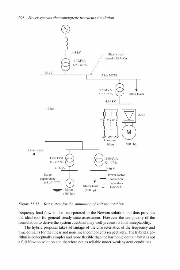
298 Power systems electromagnetic transients simulation
M
5th 7th 11th
M
Other loads
10 km
Other loads
ASD
6000 hpHarmonic
filters
Power-factorcorrectioncapacitors160 kVArMotor load
(650 hp)Motor(800 hp)
Surgecapacitance
0.5 μf
2 km MCM
144 kV
10 MVA X = 7.87 %
25 kV
4.16 kV
7.5 MVA X = 5.75 %
1500 kVA X = 4.7 %
1500 kVA X = 4.7 %
480 V4.16 kV
Short circuit Level = 75 MVA
Figure 11.15 Test system for the simulation of voltage notching
frequency load-flow is also incorporated in the Newton solution and thus providesthe ideal tool for general steady-state assessment. However the complexity of theformulation to derive the system Jacobian may well prevent its final acceptability.
The hybrid proposal takes advantage of the characteristics of the frequency andtime domains for the linear and non-linear components respectively. The hybrid algo-rithm is conceptually simpler and more flexible than the harmonic domain but it is nota full Newton solution and therefore not as reliable under weak system conditions.

Steady state applications 299
70
60
50
40
30
20
10
00 20 40 60 80 100
Impe
danc
e (Z
)
Frequency (Hz pu)
Figure 11.16 Impedance/frequency spectrum at the 25 kV bus
Simulated voltage on 25 kV system – base case
Vol
tage
(vo
lts)
3000
2000
1000
–1000
–2000
–3000
0
20 25 30 35 40Time (ms)
Figure 11.17 Simulated 25 kV system voltage with drive in operation
A direct time domain solution, particularly with the EMTP method, is the simplestand most reliable, but the least accurate due to the approximate modelling of the linearnetwork components at harmonic frequencies. The latter can be overcome with theuse of frequency dependent equivalents. A preliminary study of the linear part ofthe network provides a reduced equivalent circuit to any required matching accuracy.Then all that is needed is a single ‘brute force’ transient to steady state run followedby FFT processing of the resulting waveforms.
While there is still work to be done on the subject of frequency dependent equiv-alents, it can be confidently predicted that its final incorporation will place the
300 Power systems electromagnetic transients simulation
Voltage of 4160 volt surge capacitor – base caseV
olta
ge (
volt
s)
8000
6000
4000
2000
–2000
–4000
–6000
–8000
0
20 25 30 35 40Time (ms)
Figure 11.18 Simulated waveform at the 4.16 kV bus (surge capacitor location)
electromagnetic transient alternative in the driving seat for the assessment of powersystem harmonics.
Modelling of voltage sags and voltage interruptions requires accurate representa-tion of the dynamic characteristics of the main system components, particularly thesynchronous generators and induction motors, power electronic equipment and theirprotection and control. The EMT programs meet all these requirements adequatelyand can thus be used with confidence in the simulation of sag characteristics, theireffects and the role of sag compensation devices.
Subject to the unpredictability of the arc furnace characteristics, EMT simulationwith either deterministic or stochastic models of the arc behaviour can be used toinvestigate possible mitigation techniques. Flicker penetration can also be predictedwith these programs, although the derivation of the IEC short and long-term flickerindices is currently computationally prohibitive. However, real-time digital simulatorsshould make this task easier.
11.11 References
1 LOMBARD, X., MASHEREDJIAN, J., LEFEVRE, S. and KIENY, C.: ‘Imple-mentation of a new harmonic initialisation method in EMTP’, IEEE Transactionson Power Delivery, 1995, 10 (3), pp. 1343–42
2 PERKINS, B. K., MARTI, J. R. and DOMMEL, H. W.: ‘Nonlinear elements inthe EMTP: steady state intialisation’, IEEE Transactions on Power Apparatusand Systems, 1995, 10 (2), pp. 593–601
3 WANG, X., WOODFORD, D. A., KUFFEL, R. and WIERCKX, R.: ‘A real-timetransmission line model for a digital TNA’, IEEE Transactions on Power Delivery,1996, 11 (2), pp. 1092–7

Steady state applications 301
4 MURERE, G., LEFEVRE, S. and DO, X. D.: ‘A generalised harmonic balancedmethod for EMTP initialisation’, IEEE Transactions on Power Delivery, 1995,10 (3), pp. 1353–9
5 XU, W., MARTI, J. R. and DOMMEL, H. W.: ‘A multi-phase harmonic load-flowsolution technique’, IEEE Transactions on Power Systems, 1991, 6 (1), pp. 174–82
6 HEYDT, G. T.: ‘Electric power quality’ (Stars in a Circle Publication, WestLaFayette, 1991)
7 ARRILLAGA, J., WATSON, N. R. and CHEN, S.: ‘Power system qualityassessment’ (John Wiley, Chichester, 2000)
8 YACAMINI, R. and DE OLIVEIRA, J. C.: ‘Harmonics in multiple converter sys-tems: a generalised approach’, Proceedings of IEE on Generation, Transmissionand Distribution (Part C), 1980, 127 (2), pp. 96–106
9 SMITH, B. C., ARRILLAGA, J., WOOD, A. R. and WATSON, N. R.: ‘A reviewof iterative harmonic analysis for AC-DC power systems’, Proceedings of Inter-national Conference on Harmonics and Quality of Power (ICHQP), Las Vegas,1996, pp. 314–19
10 SMITH, B. C.: ‘A harmonic domain model for the interaction of the HVdc conver-tor with ac and dc systems’ (Ph.D. thesis, University of Canterbury, New Zealand,Private Bag 4800, Christchurch, New Zealand, 1996)
11 SEMLYEN, A., ACHA, A. and ARRILLAGA, J.: ‘Newton-type algorithms forthe harmonic phasor analysis of non-linear power circuits in periodical steadystate with special reference to magnetic non-linearities’, IEEE Transactions onPower Delivery, 1992, 7 (3), pp. 1090–9
12 SEMLYEN, A. and MEDINA, A.: ‘Computation of the periodic steady statein system with non-linear components using a hybrid time and frequencydomain methodology’, IEEE Transactions on Power Systems, 1995, 10 (3),pp. 1498–1504
13 USAOLA, J. and MAYORDOMO, J. G.: ‘Multifrequency analysis with timedomain simulation’, ETEP, 1996, 6 (1), pp. 53–9
14 SEMLYEN, A. and SHLASH, M.: ‘Principles of modular harmonic power flowmethodology’, Proceedings of IEE on Generation, Transmission and Distribution(Part C), 2000, 147 (1), pp. 1–6
15 USAOLA, J. and MAYORDOMO, J. G.: ‘Fast steady state technique for harmonicanalysis’, Proceedings of International Conference on Harmonics and Quality ofPower (ICHQP IV), 1990, Budapest, pp. 336–42
16 WATSON, N. R. and IRWIN, G. D.: ‘Electromagnetic transient simulation ofpower systems using root-matching techniques’, Proceedings IEE, Part C, 1998,145 (5), pp. 481–6
17 ANDERSON, G. W. J., ARNOLD, C. P., WATSON, N. R. and ARRILLAGA, J.:‘A new hybrid ac-dc transient stability program’, International Conference onPower Systems Transients (IPST’95), September 1995, pp. 535–40
18 SZECHTMAN, M., WESS, T. and THIO, C. V.: ‘First benchmark model forHVdc control studies’, ELECTRA, 1991, 135, pp. 55–75
19 BOLLEN, M. H. J., YALCINKAYA, G. and HAZZA, G.: ‘The use of elec-tromagnetic transient programs for voltage sag analysis’, Proceedings of 10th

302 Power systems electromagnetic transients simulation
International Conference on Harmonics and Quality of Power (ICHQP’98),Athens, October 14–16, 1998, pp. 598–603
20 GOLE, A. M. and PALAV, L.: ‘Modelling of custom power devices inPSCAD/EMTDC’, Manitoba HVdc Research Centre Journal, 1998, 11 (1)
21 WOODFORD, D. A.: ‘Flicker reduction in electric arc furnaces’, Manitoba HVdcResearch Centre Journal, 2001, 11 (7)
22 KEPPLER, T.: ‘Flicker measurement and propagation in power systems’ (Ph.D.thesis, University of Canterbury, New Zealand, Private Bag 4800, Christchurch,New Zealand, 1996)
23 TANG, L., McGRANAGHAN, M., FERRARO, R., MORGANSON, S. andHUNT, B.: ‘Voltage notching interaction caused by large adjustable speed driveson distribution systems with low short-circuit capacities’, IEEE Transactions onPower Delivery, 1996, 11 (3), pp. 1444–53
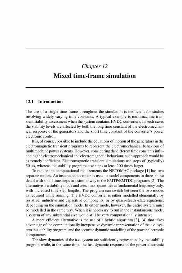
Chapter 12
Mixed time-frame simulation
12.1 Introduction
The use of a single time frame throughout the simulation is inefficient for studiesinvolving widely varying time constants. A typical example is multimachine tran-sient stability assessment when the system contains HVDC converters. In such casesthe stability levels are affected by both the long time constant of the electromechan-ical response of the generators and the short time constant of the converter’s powerelectronic control.
It is, of course, possible to include the equations of motion of the generators in theelectromagnetic transient programs to represent the electromechanical behaviour ofmultimachine power systems. However, considering the different time constants influ-encing the electromechanical and electromagnetic behaviour, such approach would beextremely inefficient. Electromagnetic transient simulations use steps of (typically)50 μs, whereas the stability programs use steps at least 200 times larger.
To reduce the computational requirements the NETOMAC package [1] has twoseparate modes. An instantaneous mode is used to model components in three-phasedetail with small time steps in a similar way to the EMTP/EMTDC programs [2]. Thealternative is a stability mode and uses r.m.s. quantities at fundamental frequency only,with increased time-step lengths. The program can switch between the two modesas required while running. The HVDC converter is either modelled elementally byresistive, inductive and capacitive components, or by quasi-steady-state equations,depending on the simulation mode. In either mode, however, the entire system mustbe modelled in the same way. When it is necessary to run in the instantaneous mode,a system of any substantial size would still be very computationally intensive.
A more efficient alternative is the use of a hybrid algorithm [3], [4] that takesadvantage of the computationally inexpensive dynamic representation of the a.c. sys-tem in a stability program, and the accurate dynamic modelling of the power electroniccomponents.
The slow dynamics of the a.c. system are sufficiently represented by the stabilityprogram while, at the same time, the fast dynamic response of the power electronic
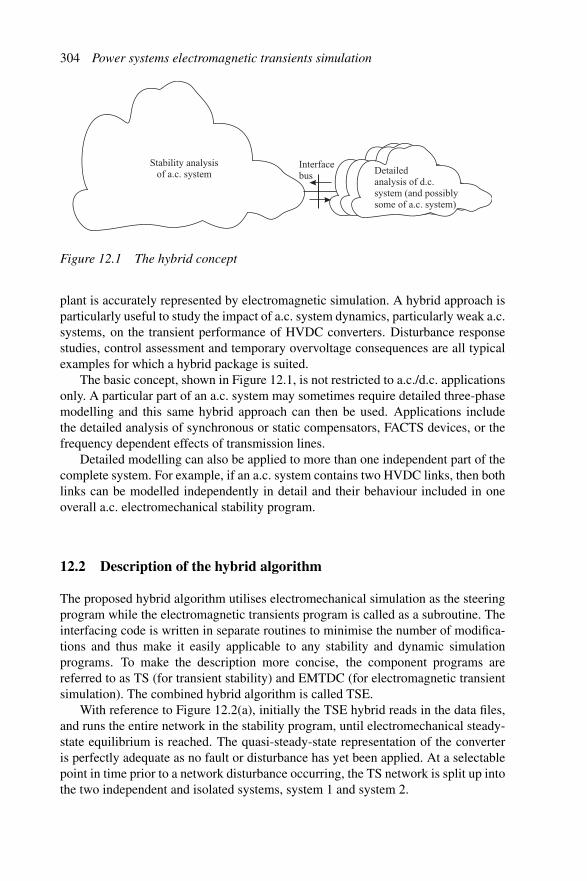
304 Power systems electromagnetic transients simulation
Stability analysis of a.c. system Detailed
analysis of d.c. system (and possibly some of a.c. system)
Interfacebus
Figure 12.1 The hybrid concept
plant is accurately represented by electromagnetic simulation. A hybrid approach isparticularly useful to study the impact of a.c. system dynamics, particularly weak a.c.systems, on the transient performance of HVDC converters. Disturbance responsestudies, control assessment and temporary overvoltage consequences are all typicalexamples for which a hybrid package is suited.
The basic concept, shown in Figure 12.1, is not restricted to a.c./d.c. applicationsonly. A particular part of an a.c. system may sometimes require detailed three-phasemodelling and this same hybrid approach can then be used. Applications includethe detailed analysis of synchronous or static compensators, FACTS devices, or thefrequency dependent effects of transmission lines.
Detailed modelling can also be applied to more than one independent part of thecomplete system. For example, if an a.c. system contains two HVDC links, then bothlinks can be modelled independently in detail and their behaviour included in oneoverall a.c. electromechanical stability program.
12.2 Description of the hybrid algorithm
The proposed hybrid algorithm utilises electromechanical simulation as the steeringprogram while the electromagnetic transients program is called as a subroutine. Theinterfacing code is written in separate routines to minimise the number of modifica-tions and thus make it easily applicable to any stability and dynamic simulationprograms. To make the description more concise, the component programs arereferred to as TS (for transient stability) and EMTDC (for electromagnetic transientsimulation). The combined hybrid algorithm is called TSE.
With reference to Figure 12.2(a), initially the TSE hybrid reads in the data files,and runs the entire network in the stability program, until electromechanical steady-state equilibrium is reached. The quasi-steady-state representation of the converteris perfectly adequate as no fault or disturbance has yet been applied. At a selectablepoint in time prior to a network disturbance occurring, the TS network is split up intothe two independent and isolated systems, system 1 and system 2.

Mixed time-frame simulation 305
Stability program
Stability program EMTDC program
Stabilityprogram
Systems 1 and 2
System 1 System 2
System 2
(a)
(b)
Figure 12.2 Example of interfacing procedure
For the sake of clarity system 1 is classified as the a.c. part of the system modelledby the stability program TS, while system 2 is the part of the system modelled in detailby EMTDC.
The snapshot data file is now used to initialise the EMTDC program used, insteadof the TS representation of system 2. The two programs are then interfaced and thenetwork disturbance can be applied. The system 2 representation in TS is isolatedbut kept up to date during the interfacing at each TS time step to allow trackingbetween programs. The a.c. network of system 1 modelled in the stability programalso supplies interface data to this system 2 network in TS as shown in Figure 12.2(b).
While the disturbance effects abate, the quasi-steady-state representation of sys-tem 2 in TS and the EMTDC representation of system 2 are tracked. If both of thesesystem 2 models produce the same results within a predefined tolerance and over a setperiod, the complete system can then be reconnected and used by TS, and the EMTDC

306 Power systems electromagnetic transients simulation
Solve EMTDC solution
Is interfacing required?
Pass information to detailed model
Solve stability equations
T = T + step length
Output results
Does T = end time?No
Stop
Extract information from detailed solution andinclude in stability program
Perform switching and subsequent bifactorisation if necessary
No
Determine stability step length
Calculate machine initial conditions
Read stability input data from load-flow results
Start
Yes
Yes
Figure 12.3 Modified TS steering routine

Mixed time-frame simulation 307
representation terminated. This allows better computational efficiency, particularlyfor long simulation runs.
12.2.1 Individual program modifications
To enable EMTDC to be called as a subroutine from TS requires a small number ofchanges to its structure. The EMTDC algorithm is split into three distinct segments,an initialising segment, the main time loop, and a termination segment. This allowsTS to call the main time loop for discrete periods as required when interfacing. TheEMTDC options, which are normally available when beginning a simulation run,are moved to the interface data file and read from there. The equivalent circuit sourcevalues, which TS updates periodically, are located in the user accessible DSDYN fileof EMTDC (described in Appendix A).
A TS program, such as the one described in reference [5], requires only minormodifications. The first is a call of the interfacing routine during the TS main timeloop as shown in Figure 12.3. The complete TS network is also split into system 1 andsystem 2 and isolated at the interface points, but this is performed in separate codeto TS. The only other direct modification inside TS is the inclusion of the interfacecurrent injections at each TS network solution.
12.2.2 Data flow
Data for the detailed EMTDC model is entered in the program database via the PSCADgraphics. Equivalent circuits are used at each interface point to represent the rest ofthe system not included in the detailed model. This system is then run until steadystate is reached and a ‘snapshot’ taken. The snapshot holds all the relevant data for thecomponents at that point in time and can be used as the starting point when interfacingthe detailed model with the stability program.
The stability program is initialised conventionally through power flow resultsvia a data file. An interface data file is also read by the TSE hybrid and containsinformation such as the number and location of interface buses, analysis options, andtiming information.
12.3 TS/EMTDC interface
Hybrid simulation requires exchange of information between the two separate pro-grams. The information that must be transferred from one program to the other mustbe sufficient to determine the power flow in or out of the interface. Possible parametersto be used are the real power P , the reactive power Q, the voltage V and the currentI at the interface (Figure 12.4). Phase angle information is also required if separatephase frames of reference are to be maintained. An equivalent circuit representingthe network modelled in the stability program is used in EMTDC and vice versa.The equivalent circuits are as shown in Figure 12.5, where E1 and Z1 represent theequivalent circuit of system 1 and Ic and Z2 the equivalent circuit of system 2.
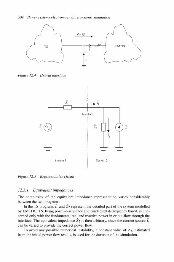
308 Power systems electromagnetic transients simulation
V
I
P + jQ
EMTDCTS
~
~
Figure 12.4 Hybrid interface
~ ~
~
~
~Z1
IC
I2
Z2E1
System 1 System 2
I1
~~V
Interface
Figure 12.5 Representative circuit
12.3.1 Equivalent impedances
The complexity of the equivalent impedance representation varies considerablybetween the two programs.
In the TS program, Ic and Z2 represent the detailed part of the system modelledby EMTDC. TS, being positive-sequence and fundamental-frequency based, is con-cerned only with the fundamental real and reactive power in or out-flow through theinterface. The equivalent impedance Z2 is then arbitrary, since the current source Ic
can be varied to provide the correct power flow.To avoid any possible numerical instability, a constant value of Z2, estimated
from the initial power flow results, is used for the duration of the simulation.

Mixed time-frame simulation 309
The EMTDC program represents system 1 by a Thevenin equivalent (E1 and Z1)as shown in Figure 12.5. The simplest Z1 is an R–L series impedance, representingthe fundamental frequency equivalent of system 1. It can be derived from the resultsof a power flow and a fault analysis at the interface bus.
The power flow provides an initial current through the interface bus and the initialinterface bus voltage. A fault analysis can easily determine the fault current throughthe interface for a short-circuit fault to ground. If the network requiring conversion toan equivalent circuit is represented by a Thevenin source E1 and Thevenin impedanceZ1, as shown in Figure 12.6, these values can thus be found as follows.
From the power flow circuit:
E1 = InZ1 + V (12.1)
and from the fault circuit:
E1 = IF Z1 (12.2)
E1~
E1~
Z1~
In~
IF~
V~
Z1~
V~
(a)
(b)
Figure 12.6 Derivation of Thevenin equivalent circuit: (a) power-flow circuit(b) fault circuit

310 Power systems electromagnetic transients simulation
Combining these two equations:
Z1 = V
IF − In
(12.3)
E1 can then be found from either equation 12.1 or 12.2.During a transient, the impedance of the synchronous machines in system 1 can
change. The net effect on the fundamental power in or out of the equivalent circuit,however, can be represented by varying the source E1 and keeping Z1 constant.
EMTDC is a ‘point on wave’ type program, and consequently involves frequen-cies other than the fundamental. A more advanced equivalent impedance capable ofrepresenting different frequencies is used in section 12.6.
12.3.2 Equivalent sources
Information from the EMTDC model representing system 2 (in Figure 12.5) is usedto modify the source of the equivalent circuit of system 2 in the stability program.Similarly, data from TS is used to modify the source of the equivalent circuit ofsystem 1 in EMTDC. These equivalent sources are normally updated at each TSstep length (refer to section 12.5). From Figure 12.5, if both Z1 and Z2 are known,additional information is still necessary to determine update values for the sources Ic
and E1. This information can be selected from the interface parameters of voltage V ,current I1, real power P , reactive power Q and power factor angle φ.
The interface voltage and current, along with the phase angle between them, areused to interchange information between programs.
12.3.3 Phase and sequence data conversions
An efficient recursive curve fitting algorithm is described in section 12.4 to extract fun-damental frequency information from the discrete point oriented waveforms producedby detailed programs such as EMTDC.
Analysis of the discrete data from EMTDC is performed over a fundamentalperiod interval, but staggered to produce results at intervals less than a fundamen-tal period. This allows the greatest accuracy in deriving fundamental results fromdistorted waveforms.
The stability program requires only positive sequence data, so data from the threea.c. phases at the interface(s) is analysed and converted to a positive sequence byconventional means. The positive sequence voltage, for example, can be derived asfollows:
Vps = 13
(Va + aVb + a2Vc
)(12.4)
whereVps = positive sequence voltageVa, Vb, Vc = phase voltagesa= 120 degree forward rotation vector (i.e. a = 1� 120◦).
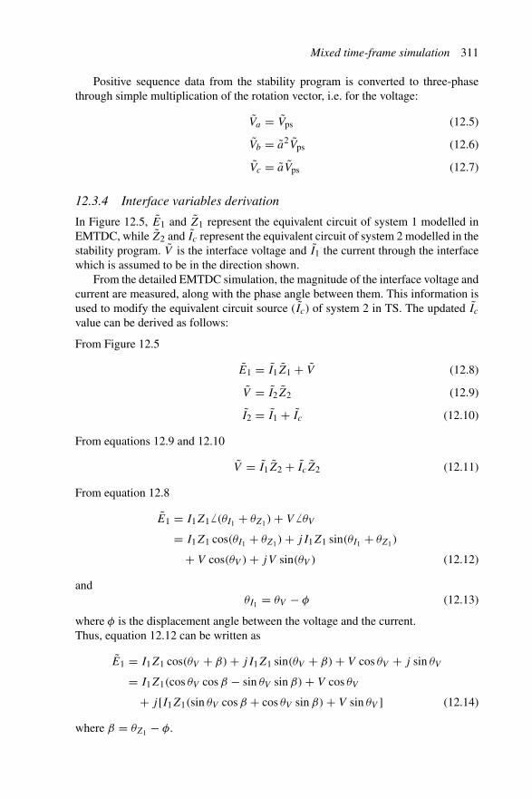
Mixed time-frame simulation 311
Positive sequence data from the stability program is converted to three-phasethrough simple multiplication of the rotation vector, i.e. for the voltage:
Va = Vps (12.5)
Vb = a2Vps (12.6)
Vc = aVps (12.7)
12.3.4 Interface variables derivation
In Figure 12.5, E1 and Z1 represent the equivalent circuit of system 1 modelled inEMTDC, while Z2 and Ic represent the equivalent circuit of system 2 modelled in thestability program. V is the interface voltage and I1 the current through the interfacewhich is assumed to be in the direction shown.
From the detailed EMTDC simulation, the magnitude of the interface voltage andcurrent are measured, along with the phase angle between them. This information isused to modify the equivalent circuit source (Ic) of system 2 in TS. The updated Ic
value can be derived as follows:
From Figure 12.5
E1 = I1Z1 + V (12.8)
V = I2Z2 (12.9)
I2 = I1 + Ic (12.10)
From equations 12.9 and 12.10
V = I1Z2 + IcZ2 (12.11)
From equation 12.8
E1 = I1Z1 � (θI1 + θZ1) + V � θV
= I1Z1 cos(θI1 + θZ1) + jI1Z1 sin(θI1 + θZ1)
+ V cos(θV ) + jV sin(θV ) (12.12)
andθI1 = θV − φ (12.13)
where φ is the displacement angle between the voltage and the current.Thus, equation 12.12 can be written as
E1 = I1Z1 cos(θV + β) + jI1Z1 sin(θV + β) + V cos θV + j sin θV
= I1Z1(cos θV cos β − sin θV sin β) + V cos θV
+ j [I1Z1(sin θV cos β + cos θV sin β) + V sin θV ] (12.14)
where β = θZ1 − φ.
312 Power systems electromagnetic transients simulation
If E1 = E1r + jE1i then equating real terms only
E1r = (I1Z1 cos(β) + V ) cos(θV ) + (−I1Z1 sin(β)) sin(θV ) (12.15)
where Z1 is known and constant throughout the simulation.From the EMTDC results, the values of V , I , and the phase difference φ are also
known and hence so is β. E1 can be determined in the TS phase reference frame fromknowledge of Z1 and the previous values of interface current and voltage from TS,through the use of equation 12.8.
From equation 12.15, making
A = I1Z1 cos(β) + V (12.16)
B = −I1Z1 sin(β) (12.17)
and remembering that
A cos(θV ) + B sin(θV ) =√
A2 + B2 cos((θV ) ± ψ) (12.18)
where(
ψ = tan−1[−B
A
])(12.19)
the voltage angle θV in the TS phase reference frame can be calculated, i.e.
θV = cos−1[
E1r√A2 + B2
]− ψ (12.20)
The equivalent current source Ic can be calculated by rearranging equation 12.11:
Ic = V
Z2
� (θV − θZ2) − I1 � θI1 (12.21)
where θI1 is obtained from equation 12.13.In a similar way, data from the transient stability program simulation can be used
to calculate a new Thevenin source voltage magnitude for the equivalent circuit ofsystem 1 in the EMTDC program. Knowing the voltage and current magnitude at theTS program interface and the phase difference between them, by a similar analysisthe voltage angle in the EMTDC phase reference frame is:
θV = cos−1[
Icr√C2 + D2
]− ψ (12.22)

Mixed time-frame simulation 313
where Icr is the real part of Ic and
C = V
Z2cos θZ2 − I1 cos φ (12.23)
D = V
Z2sin θZ2 − I1 sin φ (12.24)
φ = θV − θI1 (12.25)
ψ = tan−1[−D
C
](12.26)
Knowing the EMTDC voltage angle θV allows calculation of the EMTDC currentangle θI1 from equation 12.25. The magnitude value of E1 can then be derived fromequation 12.8.
12.4 EMTDC to TS data transfer
A significant difference between TS and EMTDC is that in TS, sinusoidal waveformsare assumed. However, during faults the EMTDC waveforms are very distorted.
The total r.m.s. power is not always equivalent to either the fundamental frequencypower nor the fundamental frequency positive sequence power. A comparison of thesethree powers following a single-phase fault at the inverter end of a d.c. link is shown inFigure 12.7. The difference between the total r.m.s. power and the positive sequencepower can be seen to be highly significant during the fault.
The most appropriate power to transfer from EMTDC to TS is then the fundamen-tal frequency positive sequence power. This, however, requires knowledge of boththe fundamental frequency positive sequence voltage and the fundamental frequencypositive sequence current. These two variables contain all the relevant informationand, hence, the use of any other power variable to transfer information becomesunnecessary.
12.4.1 Data extraction from converter waveforms
At each step of the transient stability program, power transfer information needs to bederived from the distorted converter waveforms. This can be achieved using the FFT,which provides accurate information for the whole frequency spectrum. However,only the fundamental frequency is used in the stability program and a simpler recursiveleast squares curve fitting algorithm (CFA) (described in Appendix B.5 [4]), providessufficient accuracy.
12.5 Interaction protocol
The data from each program must be interchanged at appropriate points during thehybrid simulation run. The timing of this data interchange between the TS and
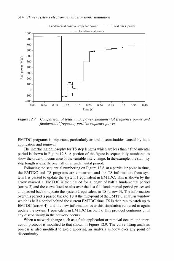
314 Power systems electromagnetic transients simulationR
eal p
ower
(M
W)
Time (s)
Fundamental positive sequence power Total r.m.s. power
Fundamental power
–200
–100
0
100
200
300
400
500
600
700
800
900
1000
0.00 0.04 0.08 0.12 0.16 0.20 0.24 0.28 0.32 0.36 0.40
Figure 12.7 Comparison of total r.m.s. power, fundamental frequency power andfundamental frequency positive sequence power
EMTDC programs is important, particularly around discontinuities caused by faultapplication and removal.
The interfacing philosophy for TS step lengths which are less than a fundamentalperiod is shown in Figure 12.8. A portion of the figure is sequentially numbered toshow the order of occurrence of the variable interchange. In the example, the stabilitystep length is exactly one half of a fundamental period.
Following the sequential numbering on Figure 12.8, at a particular point in time,the EMTDC and TS programs are concurrent and the TS information from sys-tem 1 is passed to update the system 1 equivalent in EMTDC. This is shown by thearrow marked 1. EMTDC is then called for a length of half a fundamental period(arrow 2) and the curve fitted results over the last full fundamental period processedand passed back to update the system 2 equivalent in TS (arrow 3). The informationover this period is passed back to TS at the mid-point of the EMTDC analysis windowwhich is half a period behind the current EMTDC time. TS is then run to catch up toEMTDC (arrow 4), and the new information over this simulation run used to againupdate the system 1 equivalent in EMTDC (arrow 5). This protocol continues untilany discontinuity in the network occurs.
When a network change such as a fault application or removal occurs, the inter-action protocol is modified to that shown in Figure 12.9. The curve fitting analysisprocess is also modified to avoid applying an analysis window over any point ofdiscontinuity.
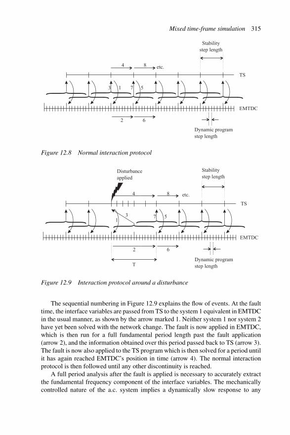
Mixed time-frame simulation 315
{{{{ { {{{
Stabilitystep length
Dynamic program step length
TS
EMTDC
etc.
1
2
3
4
5
6
7
8
Figure 12.8 Normal interaction protocol
{{{ { {{{Stabilitystep length
Dynamic program step length
Disturbanceapplied
T
TS
EMTDC
1
2
3
4
5
6
7
8 etc.
Figure 12.9 Interaction protocol around a disturbance
The sequential numbering in Figure 12.9 explains the flow of events. At the faulttime, the interface variables are passed from TS to the system 1 equivalent in EMTDCin the usual manner, as shown by the arrow marked 1. Neither system 1 nor system 2have yet been solved with the network change. The fault is now applied in EMTDC,which is then run for a full fundamental period length past the fault application(arrow 2), and the information obtained over this period passed back to TS (arrow 3).The fault is now also applied to the TS program which is then solved for a period untilit has again reached EMTDC’s position in time (arrow 4). The normal interactionprotocol is then followed until any other discontinuity is reached.
A full period analysis after the fault is applied is necessary to accurately extractthe fundamental frequency component of the interface variables. The mechanicallycontrolled nature of the a.c. system implies a dynamically slow response to any
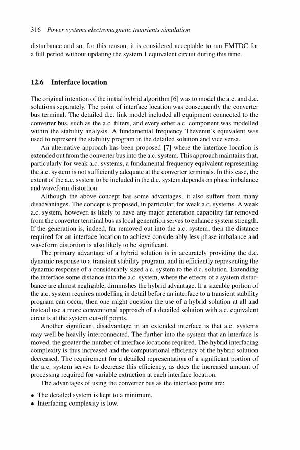
316 Power systems electromagnetic transients simulation
disturbance and so, for this reason, it is considered acceptable to run EMTDC fora full period without updating the system 1 equivalent circuit during this time.
12.6 Interface location
The original intention of the initial hybrid algorithm [6] was to model the a.c. and d.c.solutions separately. The point of interface location was consequently the converterbus terminal. The detailed d.c. link model included all equipment connected to theconverter bus, such as the a.c. filters, and every other a.c. component was modelledwithin the stability analysis. A fundamental frequency Thevenin’s equivalent wasused to represent the stability program in the detailed solution and vice versa.
An alternative approach has been proposed [7] where the interface location isextended out from the converter bus into the a.c. system. This approach maintains that,particularly for weak a.c. systems, a fundamental frequency equivalent representingthe a.c. system is not sufficiently adequate at the converter terminals. In this case, theextent of the a.c. system to be included in the d.c. system depends on phase imbalanceand waveform distortion.
Although the above concept has some advantages, it also suffers from manydisadvantages. The concept is proposed, in particular, for weak a.c. systems. A weaka.c. system, however, is likely to have any major generation capability far removedfrom the converter terminal bus as local generation serves to enhance system strength.If the generation is, indeed, far removed out into the a.c. system, then the distancerequired for an interface location to achieve considerably less phase imbalance andwaveform distortion is also likely to be significant.
The primary advantage of a hybrid solution is in accurately providing the d.c.dynamic response to a transient stability program, and in efficiently representing thedynamic response of a considerably sized a.c. system to the d.c. solution. Extendingthe interface some distance into the a.c. system, where the effects of a system distur-bance are almost negligible, diminishes the hybrid advantage. If a sizeable portion ofthe a.c. system requires modelling in detail before an interface to a transient stabilityprogram can occur, then one might question the use of a hybrid solution at all andinstead use a more conventional approach of a detailed solution with a.c. equivalentcircuits at the system cut-off points.
Another significant disadvantage in an extended interface is that a.c. systemsmay well be heavily interconnected. The further into the system that an interface ismoved, the greater the number of interface locations required. The hybrid interfacingcomplexity is thus increased and the computational efficiency of the hybrid solutiondecreased. The requirement for a detailed representation of a significant portion ofthe a.c. system serves to decrease this efficiency, as does the increased amount ofprocessing required for variable extraction at each interface location.
The advantages of using the converter bus as the interface point are:
• The detailed system is kept to a minimum.• Interfacing complexity is low.

Mixed time-frame simulation 317
• Converter terminal equipment, such as filters, synchronous condensers, SVCs, etc.can still be modelled in detail.
The major drawback of the detailed solution is in not seeing a true picture of thea.c. system, since the equivalent circuit is fundamental-frequency based. Waveformdistortion and imbalance also make it difficult to extract the fundamental frequencyinformation necessary to transfer to the stability program.
The problem of waveform distortion for transfer of data from EMTDC to TSis dependent on the accuracy of the technique for extraction of interfacing vari-able information. If fundamental-frequency quantities can be accurately measuredunder distorted conditions, then the problem is solved. Section 12.4 has describedan efficient way to extract the fundamental frequency quantities from distortedwaveforms.
Moreover, a simple fundamental frequency equivalent circuit is insufficient torepresent the correct impedance of the a.c. system at each frequency. Instead, thiscan be achieved by using a fully frequency dependent equivalent circuit of the a.c.system [8] at the converter terminal instead of just a fundamental frequency equiva-lent. A frequency dependent equivalent avoids the need for modelling any significantportion of the a.c. system in detail, yet still provides an accurate picture of the systemimpedance across its frequency spectra.
12.7 Test system and results
The test system shown in Figure 11.3 is also used here. As explained in section 12.6,the high levels of current distortion produced by the converter during the disturbancerequire a frequency dependent model of the a.c. system.
A three-phase short-circuit is applied to the rectifier terminals of the link att = 1.7 s and cleared three cycles later.
The rectifier d.c. currents, displayed for the three solutions in Figure 12.10, showa very similar variation for the TSE and EMTDC solutions, except for the regionbetween t = 2.03 s and t = 2.14 s but the difference with the TS only solution is verylarge.
Figure 12.11 compares the fundamental positive sequence real and resistivepowers across the converter interface for the TS and TSE solutions.
The main differences in real power occur during the link power ramp. The dif-ference is almost a direct relation to the d.c. current difference between TS and TSEshown in Figure 12.10. The oscillation in d.c. voltage and current as the rectifierterminal is de-blocked is also evident.
As for the reactive power Q, prior to the fault, a small amount is flowing intothe system due to surplus MVArs at the converter terminal. The fault reduces thispower flow to zero. When the fault is removed and the a.c. voltage overshoots inTSE, the reactive MVArs also overshoot in TSE and since the d.c. link is shut down,a considerable amount of reactive power flows into the system.
Finally, the machine angle swings with respect to the Clyde generator, shown inFigure 12.12, indicating that the system is transiently stable.

318 Power systems electromagnetic transients simulationD
C c
urre
nt (
pu)
EMTDC only TS only
TSE (EMTDC variable)
0.00
0.20
0.40
0.60
0.80
1.00
1.20
Time (s)
1.50 1.65 1.80 1.95 2.10 2.25 2.40 2.55 2.70 2.85 3.00
Figure 12.10 Rectifier terminal d.c. current comparisons
–200
0
200
400
600
800
1000
1200
–1400
–1200
–1000
–800
–600
–400
–200
0
200
1.50 1.65 1.80 1.95 2.10 2.25 2.40 2.55 2.70 2.85 3.00
Time (s)
1.50 1.65 1.80 1.95 2.10 2.25 2.40 2.55 2.70 2.85 3.00
Time (s)
TSE TS
TSE TS
Rea
l pow
er (
MW
)R
eact
ive
pow
er (
MV
Ar)
(a)
(b)
Figure 12.11 Real and reactive power across interface

Mixed time-frame simulation 319
Mac
hine
ang
le (
degs
)
Time (s)
–50
–30
–10
10
30
50
0.0 1.0 2.0 3.0 4.0 5.0 6.0 7.0 8.0 9.0 10.0
Roxburgh AviemoreBenmore
Figure 12.12 Machine variables – TSE (TS variables)
12.8 Discussion
It has been shown that mixed time-frame simulation requires elaborate interfacesbetween the component programs. Therefore, considering the increased cheapcomputer power availability, it would be difficult to justify its use purely in termsof computation efficiency.
The EMTP method has already proved its value in practically all types of powersystems transient. Its effectiveness has also been extended to problems involvingelectromechanical oscillations, like in the case of subsynchronous resonance.
The only possible area of application for the mixed time-frame solution is inmultimachine transient stability when the system contains HVDC transmission. Thecriterion used to decide on the prospective use of a mixed time-frame solution in thiscase is the inability of the power electronic controller to take the specified controlaction within the integration steps of the stability program. It has been shown in thechapter that the inverter behaviour of a conventional HVDC link is unpredictableduring a.c. system faults. This is caused by the occurrence of commutation failuresand by the filter’s response. Thus the effectiveness of the mixed time-frame alternativehas been clearly demonstrated for this application.
However the criterion is not met by other power electronic devices, such asFACTS. These do not suffer from commutation failures, either because they do not useinverters (e.g. thyristor controlled series capacitors, static VAR compensators, etc.)or they use turn-off switching (e.g. STATCOM and unified power flow controller).In all these cases the use of a quasi-steady-state model will be perfectly adequate forthe needs of the stability study.
12.9 References
1 KULICKE, B.: ‘NETOMAC digital program for simulating electromechani-cal and electromagnetic transient phenomena in AC power systems’, Elektriz-itätswirtschaft, 1, 1979, pp. 18–23

320 Power systems electromagnetic transients simulation
2 WOODFORD, D. A., INO, T., MATHUR, R. M., GOLE, A. M. and WIERCKX, R.:‘Validation of digital simulation of HVdc transients by field tests’, IEE ConferencePublication on AC and DC power transmission, 1985, 255, pp. 377–81
3 ANDERSON, G. W. J., ARNOLD, C. P., WATSON, N. R. and ARRILLAGA, J.:‘A new hybrid ac-dc transient stability program’, International Conference onPower Systems Transients (IPST ’95), September 1995, pp. 535–40
4 ANDERSON, G. W. J.: ‘Hybrid simulation of ac-dc power systems’ (Ph.D. the-sis, University of Canterbury, New Zealand, Private Bag 4800, Christchurch,New Zealand, 1995)
5 ARRILLAGA, J. and WATSON, N. R.: ‘Computer modelling of electrical powersystems’ (John Wiley, Chichester, 2nd edition, 2001)
6 HEFFERNAN, M. D., TURNER, K. S. and ARRILLAGA, J.: ‘Computation ofAC-DC system disturbances, parts I, II and III’, IEEE Transactions on PowerApparatus and Systems, 1981, 100 (11), pp. 4341–63
7 REEVE, J. and ADAPA, R.: ‘A new approach to dynamic analysis of AC networksincorporating detailed modelling of DC systems, part I and II’, IEEE Transactionson Power Delivery, 1988, 3 (4), pp. 2005–19
8 WATSON, N. R.: ‘Frequency-dependent A.C. system equivalents for harmonicstudies and transient convertor simulation’ (Ph.D. thesis, University of Canterbury,New Zealand, 1987)
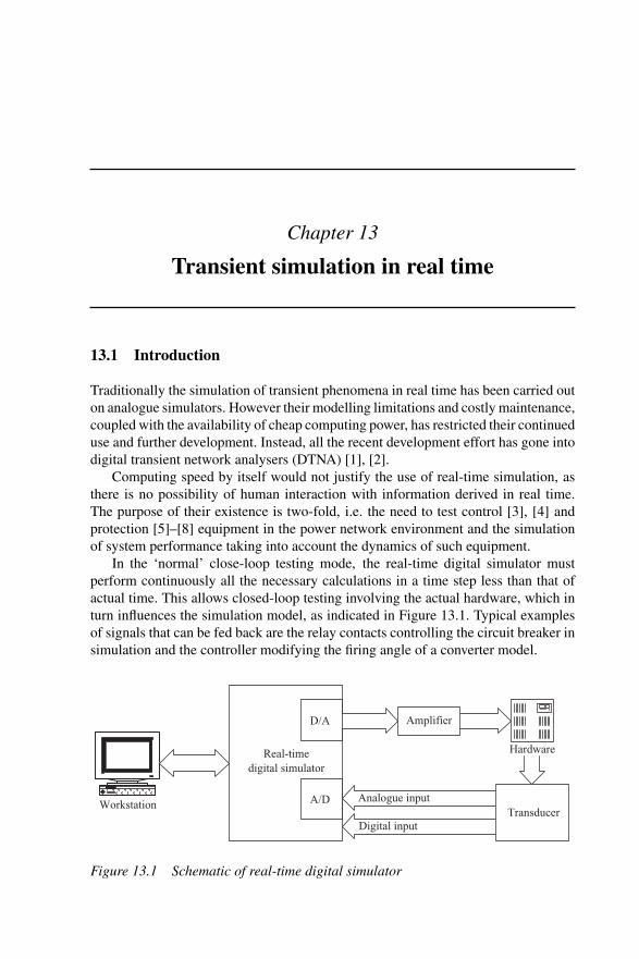
Chapter 13
Transient simulation in real time
13.1 Introduction
Traditionally the simulation of transient phenomena in real time has been carried outon analogue simulators. However their modelling limitations and costly maintenance,coupled with the availability of cheap computing power, has restricted their continueduse and further development. Instead, all the recent development effort has gone intodigital transient network analysers (DTNA) [1], [2].
Computing speed by itself would not justify the use of real-time simulation, asthere is no possibility of human interaction with information derived in real time.The purpose of their existence is two-fold, i.e. the need to test control [3], [4] andprotection [5]–[8] equipment in the power network environment and the simulationof system performance taking into account the dynamics of such equipment.
In the ‘normal’ close-loop testing mode, the real-time digital simulator mustperform continuously all the necessary calculations in a time step less than that ofactual time. This allows closed-loop testing involving the actual hardware, which inturn influences the simulation model, as indicated in Figure 13.1. Typical examplesof signals that can be fed back are the relay contacts controlling the circuit breaker insimulation and the controller modifying the firing angle of a converter model.
Real-timedigital simulator
D/A
Hardware
Analogue inputA/D
Amplifier
Digital inputTransducer
Workstation
Figure 13.1 Schematic of real-time digital simulator

322 Power systems electromagnetic transients simulation
The processing power required to solve the system equations in real time isimmense and the key to achieving it with present computer technology is the useof parallel processing. Chapter 4 has shown that the presence of transmission lines(with a travelling wave time of one time step or more) results in a block diagonalstructure of the conductance matrix, with each block being a subsystem. The prop-agation of a disturbance from one end of the line to the other is delayed by the linetravelling time. Therefore, the voltages and currents in a subsystem can be calculatedat time t without information about the voltages and currents in the other subsystemsat this time step. Thus by splitting the system into subsystems the calculations can beperformed in parallel without loss of accuracy.
Although in the present state of development DTNAs are limited in the size anddetail of system representation, they are already a considerable improvement on theconventional TNAs in this respect. The main advantages of digital over analoguesimulators are:
• Cost• Better representation of components, particularly high-frequency phenomena• Faster and easier preparation for tests• Ease and flexibility for entering new models• Better consistency (repeatability) in simulation results.
Some applications use dedicated architectures to perform the parallel processing.For instance the RTDS uses DSPs (digital signal processors) to perform the calcula-tions. However, the ever increasing processing power of computers is encouraging thedevelopment of real-time systems that will run on standard parallel computers. Even-tually this is likely to result in lower cost as well as provide portability of softwareand simplify future upgrading as computer systems advance [9].
Regardless of the type of DTNA hardware, real-time simulation requires interfac-ing with ‘physical’ equipment. The main interface components are digital to analogueconverters (DACs), amplifiers and analogue to digital converters (ADCs).
13.2 Simulation with dedicated architectures
The first commercial real-time digital simulator was released by RTDS Technologiesin 1991; an early prototype is shown in Figure 13.2. The RTDS (in the middle of thepicture) was interfaced to the controller of an HVDC converter (shown on the left)to assess its performance; the amplifiers needed to interface the digital and analogueparts are shown on the right of the picture.
However, recent developments have made it possible to achieve real-time large-scale simulation of power systems using fully digital techniques. The latter providemore capability, accuracy and flexibility at a much lower cost. The new HVDCcontrol equipment, include the phase-locked oscillator with phase limits and fre-quency correction, various inner control loops (Idc, Vdc AC overvoltage, and γ limitcontrol), control loop selection, voltage dependent current order limits (VDCOL),

Transient simulation in real time 323
Figure 13.2 Prototype real-time digital simulator
and balancing, and power trim control. An improved firing algorithm (IFA) hasalso been added to overcome the jitter effect that results when firing pulses arriveasynchronously during a time-step, as double interpolation is not used.
The largest RTDS delivered so far (to the Korean KEPCO network) simulates inreal-time (with 50 μs time step) a system of 160 buses, 41 generators, 131 transmissionlines, 78 transformers and 60 dynamic loads.
The RTDS can be operated with or without user interaction (i.e. on batch mode),whereby the equipment can be subjected to thousands of tests without supervision. Inthat mode the simulator provides detail reports on the equipment’s response to eachtest case.
The main hardware and software components of the present RTDS design arediscussed next.
13.2.1 Hardware
The RTDS architecture consists of one or more racks installed in a cubicle that alsohouse the auxiliary components (power supplies, cooling fans, . . . etc.). A rack, illus-trated in Figure 13.3, contains up to 18 processor cards and two communication cards.Currently two types of processor cards are available, i.e. the tandem processor card(TPC) and the triple processor card (3PC). Two types of communication card are alsorequired to perform the simulations, i.e. the workstation interface card (WIC) andthe inter-rack communications card (IRC). The functions of the various cards are as

324 Power systems electromagnetic transients simulation
Figure 13.3 Basic RTDS rack
follows:
Tandem processor cardThe TPC is used to perform the computations required to model the power system.One TPC contains two independent digital signal processors (DSPs) and its hardwareis not dedicated to a particular system component. Therefore, it may participate inthe modelling of a transformer in one case, while being used to model a synchronousmachine or a transmission line in another case.
Triple processor cardThe 3PC is used to model complex components, such as FACTS devices, whichcannot be modelled by a TPC. The 3PC is also used to model components whichrequire an excessive number of TPC processors. Each 3PC contains three analoguedevices (ADSP21062), based on the SHARC (Super Harvard ARchitecture) chip;these enable the board to perform approximately six times as many instructions as aTPC in any given period.
Similarly to the TPC, the function of a given processor is not component dedicated.
Inter-rack communication cardThe IRC card permits direct communications between the rack in which it is installedand up to six other racks. In a multirack simulation, the equations representing
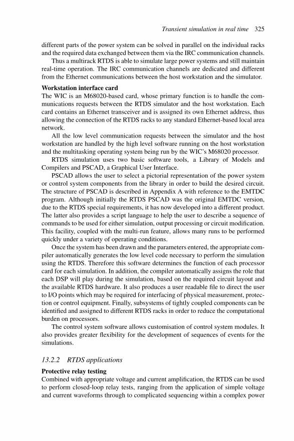
Transient simulation in real time 325
different parts of the power system can be solved in parallel on the individual racksand the required data exchanged between them via the IRC communication channels.
Thus a multirack RTDS is able to simulate large power systems and still maintainreal-time operation. The IRC communication channels are dedicated and differentfrom the Ethernet communications between the host workstation and the simulator.
Workstation interface cardThe WIC is an M68020-based card, whose primary function is to handle the com-munications requests between the RTDS simulator and the host workstation. Eachcard contains an Ethernet transceiver and is assigned its own Ethernet address, thusallowing the connection of the RTDS racks to any standard Ethernet-based local areanetwork.
All the low level communication requests between the simulator and the hostworkstation are handled by the high level software running on the host workstationand the multitasking operating system being run by the WIC’s M68020 processor.
RTDS simulation uses two basic software tools, a Library of Models andCompilers and PSCAD, a Graphical User Interface.
PSCAD allows the user to select a pictorial representation of the power systemor control system components from the library in order to build the desired circuit.The structure of PSCAD is described in Appendix A with reference to the EMTDCprogram. Although initially the RTDS PSCAD was the original EMTDC version,due to the RTDS special requirements, it has now developed into a different product.The latter also provides a script language to help the user to describe a sequence ofcommands to be used for either simulation, output processing or circuit modification.This facility, coupled with the multi-run feature, allows many runs to be performedquickly under a variety of operating conditions.
Once the system has been drawn and the parameters entered, the appropriate com-piler automatically generates the low level code necessary to perform the simulationusing the RTDS. Therefore this software determines the function of each processorcard for each simulation. In addition, the compiler automatically assigns the role thateach DSP will play during the simulation, based on the required circuit layout andthe available RTDS hardware. It also produces a user readable file to direct the userto I/O points which may be required for interfacing of physical measurement, protec-tion or control equipment. Finally, subsystems of tightly coupled components can beidentified and assigned to different RTDS racks in order to reduce the computationalburden on processors.
The control system software allows customisation of control system modules. Italso provides greater flexibility for the development of sequences of events for thesimulations.
13.2.2 RTDS applications
Protective relay testingCombined with appropriate voltage and current amplification, the RTDS can be usedto perform closed-loop relay tests, ranging from the application of simple voltageand current waveforms through to complicated sequencing within a complex power
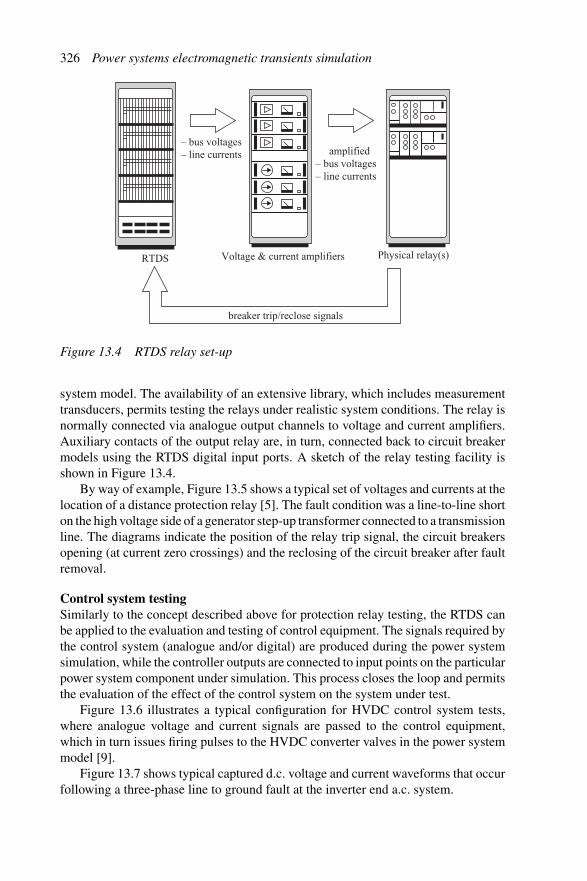
326 Power systems electromagnetic transients simulation
– bus voltages– line currents
– bus voltages– line currents
amplified
RTDS Voltage & current amplifiers Physical relay(s)
breaker trip/reclose signals
Figure 13.4 RTDS relay set-up
system model. The availability of an extensive library, which includes measurementtransducers, permits testing the relays under realistic system conditions. The relay isnormally connected via analogue output channels to voltage and current amplifiers.Auxiliary contacts of the output relay are, in turn, connected back to circuit breakermodels using the RTDS digital input ports. A sketch of the relay testing facility isshown in Figure 13.4.
By way of example, Figure 13.5 shows a typical set of voltages and currents at thelocation of a distance protection relay [5]. The fault condition was a line-to-line shorton the high voltage side of a generator step-up transformer connected to a transmissionline. The diagrams indicate the position of the relay trip signal, the circuit breakersopening (at current zero crossings) and the reclosing of the circuit breaker after faultremoval.
Control system testingSimilarly to the concept described above for protection relay testing, the RTDS canbe applied to the evaluation and testing of control equipment. The signals required bythe control system (analogue and/or digital) are produced during the power systemsimulation, while the controller outputs are connected to input points on the particularpower system component under simulation. This process closes the loop and permitsthe evaluation of the effect of the control system on the system under test.
Figure 13.6 illustrates a typical configuration for HVDC control system tests,where analogue voltage and current signals are passed to the control equipment,which in turn issues firing pulses to the HVDC converter valves in the power systemmodel [9].
Figure 13.7 shows typical captured d.c. voltage and current waveforms that occurfollowing a three-phase line to ground fault at the inverter end a.c. system.

Transient simulation in real time 327
30.0000
18.0000
6.0000
–6.0000
–18.0000
–30.0000
85.0000
51.0000
17.0000
–17.0000
–51.0000
–85.0000
Phase A Phase CPhase B
Phase A
Case 4-1 AB fault beyond transformer (d–y)
Phase CPhase BV
olta
ge (
kV)
Cur
rent
(kA
)
Figure 13.5 Phase distance relay results
– commutating bus voltages – d.c. current & voltage – valve current zero pulses
– firing pulses – block/bypass signal
. .. .
.. .. ..
RTDS HVDCcontrol system
Figure 13.6 HVDC control system testing
13.3 Real-time implementation on standard computers
This section describes a DTNA that can perform real-time tests on a standard mul-tipurpose parallel computer. The interaction between the real equipment under testand the simulated power system is carried out at every time step. A program basedon the parallel processing architecture is used to reduce the solution time [10], [11].
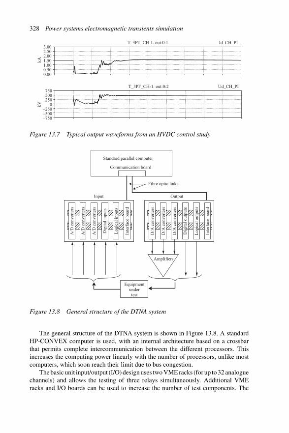
328 Power systems electromagnetic transients simulation
3.002.502.001.501.000.500.00
kAkV
750500250
0–250–500–750
T_3PT_CH-1. out:0:1
T_3PF_CH-1. out:0:2
Id_CH_PI
Ud_CH_PI
Figure 13.7 Typical output waveforms from an HVDC control study
Standard parallel computer
Communication board
Fibre optic links
OutputInput
Amplifiers
D/A
con
vert
ers
D/A
con
vert
ers
D/A
con
vert
ers
Dig
ital o
utpu
ts
Log
ical
out
puts
Inte
rfac
e bo
ard
A/D
con
vert
ers
A/D
con
vert
ers
A/D
con
vert
ers
Dig
ital i
nput
s
Log
ical
inpu
ts
Inte
rfac
e bo
ard
Equipmentundertest
Figure 13.8 General structure of the DTNA system
The general structure of the DTNA system is shown in Figure 13.8. A standardHP-CONVEX computer is used, with an internal architecture based on a crossbarthat permits complete intercommunication between the different processors. Thisincreases the computing power linearly with the number of processors, unlike mostcomputers, which soon reach their limit due to bus congestion.
The basic unit input/output (I/O) design uses two VME racks (for up to 32 analoguechannels) and allows the testing of three relays simultaneously. Additional VMEracks and I/O boards can be used to increase the number of test components. The
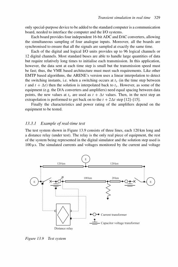
Transient simulation in real time 329
only special-purpose device to be added to the standard computer is a communicationboard, needed to interface the computer and the I/O systems.
Each board provides four independent 16-bit ADC and DAC converters, allowingthe simultaneous sampling of four analogue inputs. Moreover, all the boards aresynchronised to ensure that all the signals are sampled at exactly the same time.
Each of the digital and logical I/O units provides up to 96 logical channels or12 digital channels. Most standard buses are able to handle large quantities of databut require relatively long times to initialise each transmission. In this application,however, the data sent at each time step is small but the transmission speed mustbe fast; thus, the VME based architecture must meet such requirements. Like otherEMTP based algorithms, the ARENE’s version uses a linear interpolation to detectthe switching instants, i.e. when a switching occurs at tx (in the time step betweent and t + �t) then the solution is interpolated back to tx . However, as some of theequipment (e.g. the D/A converters and amplifiers) need equal spacing between datapoints, the new values at tx are used as t + �t values. Then, in the next step anextrapolation is performed to get back on to the t + 2�t step [12]–[15].
Finally the characteristics and power rating of the amplifiers depend on theequipment to be tested.
13.3.1 Example of real-time test
The test system shown in Figure 13.9 consists of three lines, each 120 km long anda distance relay (under test). The relay is the only real piece of equipment, the restof the system being represented in the digital simulator and the solution step used is100 μs. The simulated currents and voltages monitored by the current and voltage
E
EE
120 km 120 km
20 km100 km
Distance relay
Current transformer
Capacitor voltage transformer
Figure 13.9 Test system
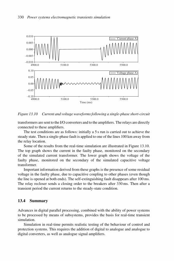
330 Power systems electromagnetic transients simulation
Current phase A
Voltage phase A
0.010
0.005
0.000
–0.005
–0.010
0.10
0.05
0.00
–0.05
–0.10
4900.0 5100.0 5300.0 5500.0
4900.0 5100.0 5300.0 5500.0Time (ms)
Figure 13.10 Current and voltage waveforms following a single-phase short-circuit
transformers are sent to the I/O converters and to the amplifiers. The relays are directlyconnected to these amplifiers.
The test conditions are as follows: initially a 5 s run is carried out to achieve thesteady state. Then a single-phase fault is applied to one of the lines 100 km away fromthe relay location.
Some of the results from the real-time simulation are illustrated in Figure 13.10.The top graph shows the current in the faulty phase, monitored on the secondaryof the simulated current transformer. The lower graph shows the voltage of thefaulty phase, monitored on the secondary of the simulated capacitive voltagetransformer.
Important information derived from these graphs is the presence of some residualvoltage in the faulty phase, due to capacitive coupling to other phases (even thoughthe line is opened at both ends). The self-extinguishing fault disappears after 100 ms.The relay recloser sends a closing order to the breakers after 330 ms. Then after atransient period the current returns to the steady-state condition.
13.4 Summary
Advances in digital parallel processing, combined with the ability of power systemsto be processed by means of subsystems, provides the basis for real-time transientsimulation.
Simulation in real-time permits realistic testing of the behaviour of control andprotection systems. This requires the addition of digital to analogue and analogue todigital converters, as well as analogue signal amplifiers.
Transient simulation in real time 331
The original, and at present still the main application in the market, is a simula-tor based on dedicated architecture called RTDS (real-time digital simulator). Thisunit practically replaced all the scale-down physical simulators and can potentiallyrepresent any size system,
The development of multipurpose parallel computing is now providing the basisfor real-time simulation using standard computers instead of dedicated architectures,and should eventually provide a more economical solution.
13.5 References
1 KUFFEL, P., GIESBRECHT, J., MAGUIRE, T., WIERCKX, R. P. andMcLAREN, P.: ‘RTDS – a fully digital power system simulator operating inreal-time’, Proceedings of the ICDS Conference, College Station, Texas, USA,April 1995, pp. 19–24
2 WIERCKX, R. P.: ‘Fully digital real time electromagnetic transient simula-tor’, IERE Workshop on New Issues in Power System Simulation, 1992, VII,pp. 128–228
3 BRANDT, D., WACHAL, R., VALIQUETTE, R. and WIERCKX, R. P.: ‘Closedloop testing of a joint VAr controller using a digital real-time simulator for HVdcsystem and control studies’, IEEE Transactions on Power Systems, 1991, 6 (3),pp. 1140–6.
4 WIERCKX, R. P., GIESBRECHT W. J., KUFFEL, R. et al.: ‘Validation of a fullydigital real time electromagnetic transient simulator for HVdc system and controlstudies’, Proceedings of the Athens Power Tech. Conference, September 1993,pp. 751–9
5 McLAREN, P. G., KUFFEL, R., GIESBRECHT, W. J., WIERCKX, R. P. andARENDT, L.: ‘A real time digital simulator for testing relays’, IEEE Transactionson Power Delivery, January 1992, 7 (1), pp. 207–13
6 KUFFEL, R., McLAREN, P., YALLA, M. and WANG, X.: ‘Testing of theBeckwith electric M-0430 multifunction protection relay using a real-time digitalsimulator (RTDS)’, Proceedings of International Conference on Digital PowerSystem Simulators (ICDS), College Station, Texas, USA, April 1995, pp. 49–54.
7 McLAREN, P., DIRKS, R. P., JAYASINGHE, R. P., SWIFT, G. W. andZHANG, Z.: ‘Using a real time digital simulator to develop an accurate model ofa digital relay’, Proceedings of International Conference on Digital Power SystemSimulators, ICDS’95, April 1995, p. 173
8 McLAREN, P., SWIFT, G. W., DIRKS, R. P. et al.: ‘Comparisons of relaytransient test results using various testing technologies’, Proceedings of Sec-ond International Conference on Digital Power System Simulators, ICDS’97,May 1997, pp. 57–62
9 DUCHEN, H., LAGERKVIST, M., KUFFEL, R. and WIERCKX, R.: ‘HVDCsimulation and control system testing using a real-time digital simulator (RTDS)’,Proceedings of the ICDS Conference, College Station, Texas, USA, April 1995,p. 213
332 Power systems electromagnetic transients simulation
10 STRUNZ, K. and MULLER, S.: ‘New trends in protective relay testing’, Proceed-ings of Fifth International Power Engineering Conference (IPEC), May 2001, 1,pp. 456–60
11 STRUNZ, K., MARTINOLE, P., MULLER, S. and HUET, O.: ‘Control systemtesting in electricity market places’, Proceedings of Fifth International PowerEngineering Conference (IPEC), May 2001
12 STRUNZ, K., LOMBARD, X., HUET, O., MARTI, J. R., LINARES, L.and DOMMEL, H. W.: ‘Real time nodal analysis-based solution techniquesfor simulations of electromagnetic transients in power electronic systems’,Proceedings of Thirteenth Power System Computation Conference (PSCC),June 1999, Trondheim, Norway, pp. 1047–53
13 STRUNZ, K. and FROMONT, H.: ‘Exact modelling of interaction between gatepulse generators and power electronic switches for digital real time simula-tors’, Proceedings of Fifth Brazilian Power Electronics Conference (COBEP),September 1999, pp. 203–8
14 STRUNZ, K., LINARES, L., MARTI, J. R., HUET, O. and LOMBARD, X.:‘Efficient and accurate representation of asynchronous network structure changingphenomena in digital real time simulators’, IEEE Transactions on Power Systems,2000, 15 (2), pp. 586–92
15 STRUNZ, K.: ‘Real time high speed precision simulators of HDC extinctionadvance angle’, Proceedings of International Conference on Power SystemsTechnology (PowerCon2000), December 2000, pp. 1065–70

Appendix A
Structure of the PSCAD/EMTDC program
PSCAD/EMTDC version 2 consists of a set of programs which enable the efficientsimulation of a wide variety of power system networks. EMTDC (ElectromagneticTransient and DC) [1], [2], although based on the EMTP method, introduced a numberof modifications so that switching discontinuities could be accommodated accuratelyand quickly [3], the primary motivation being the simulation of HVDC systems.PSCAD (Power Systems Computer Aided Design) is a graphical Unix-based userinterface for the EMTDC program. PSCAD consists of software enabling the user toenter a circuit graphically, create new custom components, solve transmission lineand cable parameters, interact with an EMTDC simulation while in progress and toprocess the results of a simulation [4].
The programs comprising PSCAD version 2 are interfaced by a large numberof data files which are managed by a program called FILEMANAGER. This pro-gram also provides an environment within which to call the other five programs andto perform housekeeping tasks associated with the Unix system, as illustrated inFigure A.1. The starting point for any study with EMTDC is to create a graphicalsketch of the circuit to be solved using the DRAFT program. DRAFT provides theuser with a canvas area and a selection of component libraries (shown in Figure A.2).
Filemanager
Cable TLine Draft Runtime
EMTDC
UniPlot MultiPlot
Figure A.1 The PSCAD/EMTDC Version 2 suite

334 Power systems electromagnetic transients simulation
Figure A.2 DRAFT program
A library is a set of component icons, any of which can be dragged to the canvasarea and connected to other components by bus-work icons. Associated with eachcomponent icon is a form into which component parameters can be entered. Theuser can create component icons, the forms to go with them and FORTRAN code todescribe how the component acts dynamically in a circuit. Typical components aremulti-winding transformers, six-pulse groups, control blocks, filters, synchronousmachines, circuit-breakers, timing logic, etc.
The output from DRAFT is a set of files which are used by EMTDC. EMTDCis called from the PSCAD RUNTIME program, which permits interactions with thesimulation while it is in progress. Figure A.3 shows RUNTIME plotting the outputvariables as EMTDC simulates. RUNTIME enables the user to create buttons, slides,dials and plots connected to variables used as input or output to the simulation (shownin Figure A.4). At the end of simulation, RUNTIME copies the time evolution ofspecified variables into data files. The complete state of the system at the end ofsimulation can also be copied into a snapshot file, which can then be used as thestarting point for future simulations. The output data files from EMTDC can be plottedand manipulated by the plotting programs UNIPLOT or MULTIPLOT. MULTIPLOTallows multiple pages to be laid out, with multiple plots per page and the results fromdifferent runs shown together. Figure A.5 shows a MULTIPLOT display of the resultsfrom two different simulations. A calculator function and off-line DFT function are
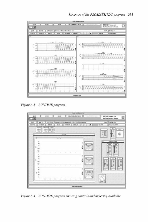
Structure of the PSCAD/EMTDC program 335
Figure A.3 RUNTIME program
Figure A.4 RUNTIME program showing controls and metering available
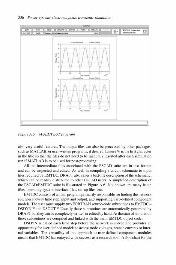
336 Power systems electromagnetic transients simulation
Figure A.5 MULTIPLOT program
also very useful features. The output files can also be processed by other packages,such as MATLAB, or user-written programs, if desired. Ensure % is the first characterin the title so that the files do not need to be manually inserted after each simulationrun if MATLAB is to be used for post-processing.
All the intermediate files associated with the PSCAD suite are in text formatand can be inspected and edited. As well as compiling a circuit schematic to inputfiles required by EMTDC, DRAFT also saves a text-file description of the schematic,which can be readily distributed to other PSCAD users. A simplified description ofthe PSCAD/EMTDC suite is illustrated in Figure A.6. Not shown are many batchfiles, operating system interface files, set-up files, etc.
EMTDC consists of a main program primarily responsible for finding the networksolution at every time step, input and output, and supporting user-defined componentmodels. The user must supply two FORTRAN source-code subroutines to EMTDC –DSDYN.F and DSOUT.F. Usually these subroutines are automatically generated byDRAFT but they can be completely written or edited by hand. At the start of simulationthese subroutines are compiled and linked with the main EMTDC object code.
DSDYN is called each time step before the network is solved and provides anopportunity for user-defined models to access node voltages, branch currents or inter-nal variables. The versatility of this approach to user-defined component modulesmeans that EMTDC has enjoyed wide success as a research tool. A flowchart for the
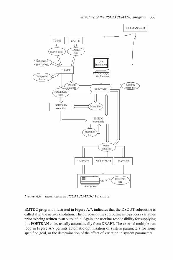
Structure of the PSCAD/EMTDC program 337
TLINE
FILEMANAGER
Componentlibraries
Schematicdescription
FORTRANcompiler
Snapshotfile
Workstation
UserInteraction
UNIPLOT MATLAB
Runtimebatch file
CABLE
DRAFT
Systemdata file
Make file
FORTRANfiles
EMTDCexecutable
outputdatafiles
RUNTIME
Laser printer
postscriptfile
MULTIPLOT
OR
CABLEdataTLINE data
Figure A.6 Interaction in PSCAD/EMTDC Version 2
EMTDC program, illustrated in Figure A.7, indicates that the DSOUT subroutine iscalled after the network solution. The purpose of the subroutine is to process variablesprior to being written to an output file. Again, the user has responsibility for supplyingthis FORTRAN code, usually automatically from DRAFT. The external multiple-runloop in Figure A.7 permits automatic optimisation of system parameters for somespecified goal, or the determination of the effect of variation in system parameters.
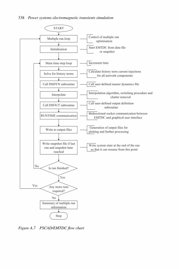
338 Power systems electromagnetic transients simulation
Yes
No
Yes
No
Start EMTDC from data file or snapshot
Control of multiple runoptimisation
Increment time
Calculate history term current injections for all network components
Call user-defined master dynamics file
Interpolation algorithm, switching procedure andchatter removal
Call user-defined output definition subroutine
Bidirectional socket communication between EMTDC and graphical user interface
Generation of output files for plotting and further processing
Write system state at the end of the run so that it can resume from this point
Stop
Multiple run loop
Is run finished?
START
Initialisation
Main time-step loop
Solve for history terms
Call DSDYN subroutine
Interpolate
Call DSOUT subroutine
Write to output files
Any more runs required?
Write snapshot file if last run and snapshot time
reached
RUNTIME communication
Summary of multiple run information
Figure A.7 PSCAD/EMTDC flow chart

Structure of the PSCAD/EMTDC program 339
The main component models used in EMTDC, i.e. transmission lines, syn-chronous generators and transformers, as well as control and switching modellingtechniques, have already been discussed in previous chapters.
Due to the popularity of the WINDOWS operating system on personal comput-ers, a complete rewrite of the successful UNIX version was performed, resulting inPSCAD version 3. New features include:
• The function of DRAFT and RUNTIME has been combined so that plots are puton the circuit schematic (as shown in Figure A.8).
• The new graphical user interface also supports: hierarchical design of circuit pagesand localised data generation only for modified pages, single-line diagram dataentry, direct plotting of all simulation voltages, currents and control signals, withoutwriting to output files and more flexible multiple-run control.
• A MATLAB to PSCAD/EMTDC interface has been developed. The interfaceenables controls or devices to be developed in MATLAB, and then connected inany sequence to EMTDC components. Full access to the MATLAB toolboxes willbe supported, as well as the full range of MATLAB 2D and 3D plotting commands.
• EMTDC V3 includes ideal switches with zero resistance, ideal voltage sources,improved storage methods and faster switching operations. Fortran 90/95 will begiven greater support.
• A new solution algorithm (the root-matching technique) is implemented for controlcircuits which eliminates the errors due to trapezoidal integration but which is stillnumerically stable.
Figure A.8 PSCAD Version 3 interface

340 Power systems electromagnetic transients simulation
• New transmission-line and cable models using the phase domain (as opposed tomodal domain) techniques coupled with more efficient curve fitting algorithmshave been implemented, although the old models are available for compatibilitypurposes.
To date an equivalent for the very powerful MULTIPLOT post-processing programis not available, necessitating exporting to MATLAB for processing and plotting.
PSCAD version 2 had many branch quantities that were accessed using the nodenumbers of its terminals (e.g. CDC, EDC, GDC, CCDC, etc.). These have beenreplaced by arrays (GEQ, CBR, EBR, CCBR, etc.) that are indexed by branch num-bers. For example CBR(10,2) is the 10th branch in subsystem 2. This allows aninfinite number of branches in parallel whereas version 2 only allowed three switchedbranches in parallel. Version 2 had a time delay in the plotting of current through indi-vidual parallel switches (only in plotting but not in calculations). This was because themain algorithm only computed the current through all the switches in parallel, and theallocation of current in individual switches was calculated from a subroutine calledfrom DSDYN. Old version 2 code can still run on version 3, as interface functionshave been developed that scan through all branches until a branch with the correctsending and receiving nodes is located. Version 2 code that modifies the conductancematrix GDC directly needs to be manually changed to GEQ.
Version 4 of PSCAD/EMTDC is at present being developed. In version 3 a circuitcan be split into subpages using page components on the main page. If there areten page components on the main page connected by transmission lines or cables,then there will be ten subsystems regardless of the number of subpages branchingoff other pages. Version 4 has a new single line diagram capability as well as a newtransmission line and cable interface consisting of one object, instead of the threecurrently used (sending end, receiving end and line constants information page). Themain page will show multiple pages with transmission lines directly connected toelectrical connections on the subpage components. PSCAD will optimally determinethe subsystem splitting and will form subsystems wherever possible.
A.1 References
1 WOODFORD, D. A., INO, T., MATHUR, R. M., GOLE, A. M. and WIERCKX, R.:‘Validation of digital simulation of HVdc transients by field tests’, IEE ConferencePublication on AC and DC power transmission, 1985, 255, pp. 377–81
2 WOODFORD, D. A., GOLE, A. M. and MENZIES, R. W.: ‘Digital simulation ofDC links and AC machines’, IEEE Transactions on Power Apparatus and Systems,1983, 102 (6), pp. 1616–23
3 KUFFEL, P., KENT, K. and IRWIN, G. D.: ‘The implementation and effectivenessof linear interpolation within digital simulation’, Electrical Power and EnergySystems, 1997, 19 (4), pp. 221–4
4 Manitoba HVdc Research Centre: ‘PSCAD/EMTDC power systems simulationsoftware tutorial manual’, 1994

Appendix B
System identification techniques
B.1 s-domain identification (frequency domain)
The rational function in s to be fitted to the frequency domain data is:
H(s) = a0 + a1s1 + a2s
2 + · · · + ansN
1 + b1s1 + b2s2 + · · · + bnsn(B.1)
where N ≤ n.The frequency response of equation B.1 is:
H(jω) =∑N
k=0(ak(jω)k)∑n
k=0(bk(jω)k)(B.2)
where b0 = 1.Letting the sample data be c(jω)+jd(jω), and equating it to equation B.2 yields
c(jω) + jd(jω) =(a0 − a2ω
2k + a4ω
4k − · · · ) + j
(a1ωk − a3ω
3k − a5ω
5k − · · · )
(1 − b2ω
2k + b4ω
4k − · · · ) + j
(b1ωk − b3ω
3k − b5ω
5k − · · · )
(B.3)or
(c(jω) + jd(jω))((
1 − b2ω2k + b4ω
4k − · · · ) + j
(b1ωk − b3ω
3k − b5ω
5k − · · · ))
= (a0 − a2ω
2k + a4ω
4k − · · · ) + j
(a1ωk − a3ω
3k − a5ω
5k − · · · )
(B.4)Splitting into real and imaginary parts yields:
−dk(jω) · (b1ωk − b3ω3k − b5ω
5k − · · · ) + c(jω)
(b2ω
2k + b4ω
4k − · · · )
− (a0 − a2ω
2k + a4ω
4k − · · · ) = −c(jω)
dk(jω) · (−b2ω2k + b4ω
4k − · · · ) + c(jω) · (b1ωk − b3ω
3k − b5ω
5k − · · · )
− (a1ωk − a3ω
3k − a5ω
5k − · · · ) = −d(jω)
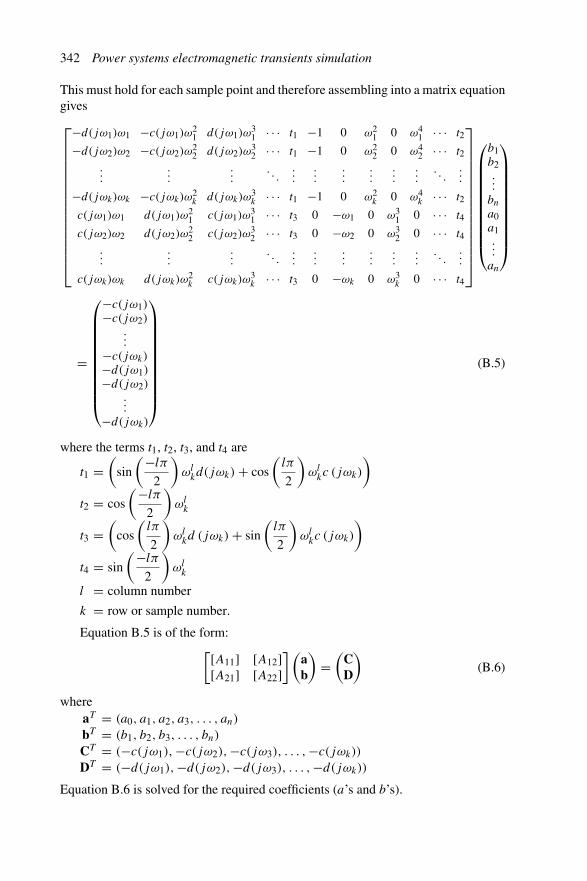
342 Power systems electromagnetic transients simulation
This must hold for each sample point and therefore assembling into a matrix equationgives
⎡
⎢⎢⎢⎢⎢⎢⎢⎢⎢⎢⎢⎢⎢⎢⎣
−d(jω1)ω1 −c(jω1)ω21 d(jω1)ω
31 · · · t1 −1 0 ω2
1 0 ω41 · · · t2
−d(jω2)ω2 −c(jω2)ω22 d(jω2)ω
32 · · · t1 −1 0 ω2
2 0 ω42 · · · t2
......
.... . .
......
......
......
. . ....
−d(jωk)ωk −c(jωk)ω2k d(jωk)ω
3k · · · t1 −1 0 ω2
k 0 ω4k · · · t2
c(jω1)ω1 d(jω1)ω21 c(jω1)ω
31 · · · t3 0 −ω1 0 ω3
1 0 · · · t4
c(jω2)ω2 d(jω2)ω22 c(jω2)ω
32 · · · t3 0 −ω2 0 ω3
2 0 · · · t4
......
.... . .
......
......
......
. . ....
c(jωk)ωk d(jωk)ω2k c(jωk)ω
3k · · · t3 0 −ωk 0 ω3
k 0 · · · t4
⎤
⎥⎥⎥⎥⎥⎥⎥⎥⎥⎥⎥⎥⎥⎥⎦
⎛
⎜⎜⎜⎜⎜⎜⎜⎜⎜⎜⎝
b1b2...
bn
a0a1...
an
⎞
⎟⎟⎟⎟⎟⎟⎟⎟⎟⎟⎠
=
⎛
⎜⎜⎜⎜⎜⎜⎜⎜⎜⎜⎝
−c(jω1)−c(jω2)
...−c(jωk)−d(jω1)−d(jω2)
...−d(jωk)
⎞
⎟⎟⎟⎟⎟⎟⎟⎟⎟⎟⎠
(B.5)
where the terms t1, t2, t3, and t4 are
t1 =(
sin
(−lπ
2
)ωl
kd(jωk) + cos
(lπ
2
)ωl
kc (jωk)
)
t2 = cos
(−lπ
2
)ωl
k
t3 =(
cos
(lπ
2
)ωl
kd (jωk) + sin
(lπ
2
)ωl
kc (jωk)
)
t4 = sin
(−lπ
2
)ωl
k
l = column number
k = row or sample number.
Equation B.5 is of the form:[[A11] [A12][A21] [A22]
](ab
)=
(CD
)(B.6)
whereaT = (a0, a1, a2, a3, . . . , an)
bT = (b1, b2, b3, . . . , bn)
CT = (−c(jω1), −c(jω2), −c(jω3), . . . ,−c(jωk))
DT = (−d(jω1), −d(jω2), −d(jω3), . . . ,−d(jωk))
Equation B.6 is solved for the required coefficients (a’s and b’s).
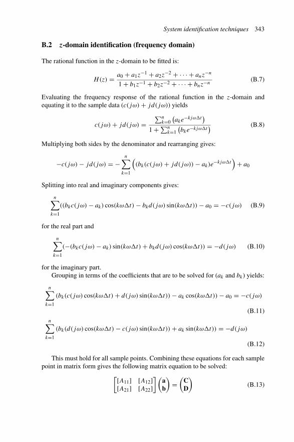
System identification techniques 343
B.2 z-domain identification (frequency domain)
The rational function in the z-domain to be fitted is:
H(z) = a0 + a1z−1 + a2z
−2 + · · · + anz−n
1 + b1z−1 + b2z−2 + · · · + bnz−n(B.7)
Evaluating the frequency response of the rational function in the z-domain andequating it to the sample data (c(jω) + jd(jω)) yields
c(jω) + jd(jω) =∑n
k=0
(ake
−kjω�t)
1 + ∑nk=1
(bke−kjω�t
) (B.8)
Multiplying both sides by the denominator and rearranging gives:
−c(jω) − jd(jω) = −n∑
k=1
((bk(c(jω) + jd(jω)) − ak)e
−kjω�t)
+ a0
Splitting into real and imaginary components gives:
n∑
k=1
((bkc(jω) − ak) cos(kω�t) − bkd(jω) sin(kω�t)) − a0 = −c(jω) (B.9)
for the real part and
n∑
k=1
(−(bkc(jω) − ak) sin(kω�t) + bkd(jω) cos(kω�t)) = −d(jω) (B.10)
for the imaginary part.Grouping in terms of the coefficients that are to be solved for (ak and bk) yields:
n∑
k=1
(bk(c(jω) cos(kω�t) + d(jω) sin(kω�t)) − ak cos(kω�t)) − a0 = −c(jω)
(B.11)
n∑
k=1
(bk(d(jω) cos(kω�t) − c(jω) sin(kω�t)) + ak sin(kω�t)) = −d(jω)
(B.12)
This must hold for all sample points. Combining these equations for each samplepoint in matrix form gives the following matrix equation to be solved:
[[A11] [A12][A21] [A22]
](ab
)=
(CD
)(B.13)
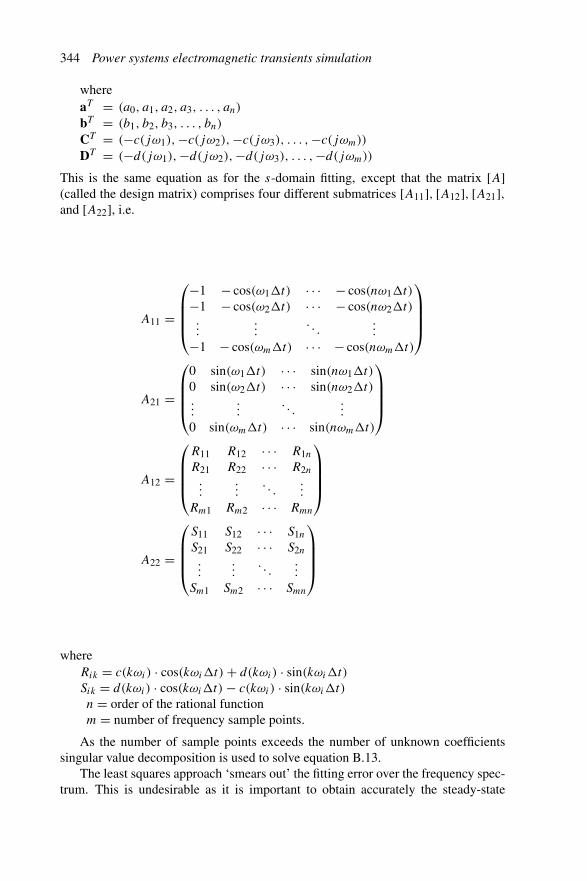
344 Power systems electromagnetic transients simulation
whereaT = (a0, a1, a2, a3, . . . , an)
bT = (b1, b2, b3, . . . , bn)
CT = (−c(jω1), −c(jω2), −c(jω3), . . . ,−c(jωm))
DT = (−d(jω1), −d(jω2), −d(jω3), . . . ,−d(jωm))
This is the same equation as for the s-domain fitting, except that the matrix [A](called the design matrix) comprises four different submatrices [A11], [A12], [A21],and [A22], i.e.
A11 =
⎛
⎜⎜⎜⎝
−1 − cos(ω1�t) · · · − cos(nω1�t)
−1 − cos(ω2�t) · · · − cos(nω2�t)...
.... . .
...
−1 − cos(ωm�t) · · · − cos(nωm�t)
⎞
⎟⎟⎟⎠
A21 =
⎛
⎜⎜⎜⎝
0 sin(ω1�t) · · · sin(nω1�t)
0 sin(ω2�t) · · · sin(nω2�t)...
.... . .
...
0 sin(ωm�t) · · · sin(nωm�t)
⎞
⎟⎟⎟⎠
A12 =
⎛
⎜⎜⎜⎝
R11 R12 · · · R1n
R21 R22 · · · R2n
......
. . ....
Rm1 Rm2 · · · Rmn
⎞
⎟⎟⎟⎠
A22 =
⎛
⎜⎜⎜⎝
S11 S12 · · · S1n
S21 S22 · · · S2n
......
. . ....
Sm1 Sm2 · · · Smn
⎞
⎟⎟⎟⎠
whereRik = c(kωi) · cos(kωi�t) + d(kωi) · sin(kωi�t)
Sik = d(kωi) · cos(kωi�t) − c(kωi) · sin(kωi�t)
n = order of the rational functionm = number of frequency sample points.
As the number of sample points exceeds the number of unknown coefficientssingular value decomposition is used to solve equation B.13.
The least squares approach ‘smears out’ the fitting error over the frequency spec-trum. This is undesirable as it is important to obtain accurately the steady-state
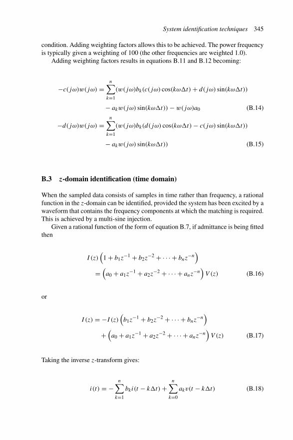
System identification techniques 345
condition. Adding weighting factors allows this to be achieved. The power frequencyis typically given a weighting of 100 (the other frequencies are weighted 1.0).
Adding weighting factors results in equations B.11 and B.12 becoming:
−c(jω)w(jω) =n∑
k=1
(w(jω)bk(c(jω) cos(kω�t) + d(jω) sin(kω�t))
− akw(jω) sin(kω�t)) − w(jω)a0 (B.14)
−d(jω)w(jω) =n∑
k=1
(w(jω)bk(d(jω) cos(kω�t) − c(jω) sin(kω�t))
− akw(jω) sin(kω�t)) (B.15)
B.3 z-domain identification (time domain)
When the sampled data consists of samples in time rather than frequency, a rationalfunction in the z-domain can be identified, provided the system has been excited by awaveform that contains the frequency components at which the matching is required.This is achieved by a multi-sine injection.
Given a rational function of the form of equation B.7, if admittance is being fittedthen
I (z)(
1 + b1z−1 + b2z
−2 + · · · + bnz−n
)
=(a0 + a1z
−1 + a2z−2 + · · · + anz
−n)
V (z) (B.16)
or
I (z) = −I (z)(b1z
−1 + b2z−2 + · · · + bnz
−n)
+(a0 + a1z
−1 + a2z−2 + · · · + anz
−n)
V (z) (B.17)
Taking the inverse z-transform gives:
i(t) = −n∑
k=1
bki(t − k�t) +n∑
k=0
akv(t − k�t) (B.18)

346 Power systems electromagnetic transients simulation
and in matrix form⎡
⎢⎢⎢⎣
v(t1) v(t1 − �t) v(t1 − 2�t) · · · v(t1 − n�t) −i(t1 − �t) −i(t1 − 2�t) · · · i(t1 − n�t)
v(t2) v(t2 − �t) v(t2 − 2�t) · · · v(t2 − n�t) −i(t2 − �t) −i(t2 − 2�t) · · · i(t2 − n�t)
......
......
......
...
v(tk) v(tk − �t) v(tk − 2�t) · · · v(tk − n�t) −i(tk − �t) −i(tk − 2�t) · · · i(tk − n�t)
⎤
⎥⎥⎥⎦
×
⎛
⎜⎜⎜⎜⎜⎜⎜⎜⎜⎜⎜⎜⎜⎝
a0a1...
an
b1b2...
bn
⎞
⎟⎟⎟⎟⎟⎟⎟⎟⎟⎟⎟⎟⎟⎠
=
⎛
⎜⎜⎜⎝
i(t1)
i(t2)
...
i(tk)
⎞
⎟⎟⎟⎠
(B.19)
wherek = time sample numbern = order of the rational function (k > p, i.e. over-sampled).
The time step must be chosen sufficiently small to avoid aliasing, i.e. �t =1/ (K1fmax), where K1 > 2 (Nyquist criteria) and fmax is the highest frequencyinjected. For instance if K1 = 10 and �t = 50 μs there will be 4000 samplespoints per cycle (20 ms for 50 Hz). This equivalent is easily extended to multi-portequivalents [1]. For an m-port equivalent there will be m(m+ 1)/2 rational functionsto be fitted.
B.4 Prony analysis
Prony analysis identifies a rational function that will have a prescribed time-domainresponse [2]. Given the rational function:
H(z) = Y (z)
U(z)= a0 + a1z
−1 + a2z−2 + · · · + anz
−N
1 + b1z−1 + b2z−2 + · · · + bdz−n(B.20)
the impulse response of h(k) is related to H(z) by the z-transform, i.e.
H(z) =∞∑
k=0
h(k)z−1 (B.21)
which can be written as
Y (z)(
1 + b1z−1 + b2z
−2 + · · · + bdz−n)
= U(z)(a0 + a1z
−1 + a2z−2 + · · · + anz
−N)
(B.22)
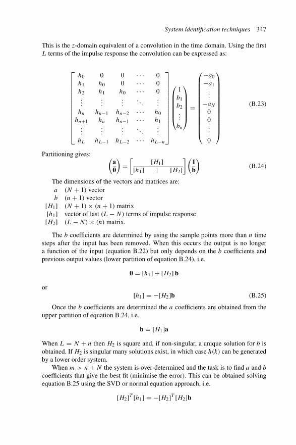
System identification techniques 347
This is the z-domain equivalent of a convolution in the time domain. Using the firstL terms of the impulse response the convolution can be expressed as:
⎡
⎢⎢⎢⎢⎢⎢⎢⎢⎢⎢⎢⎢⎣
h0 0 0 · · · 0h1 h0 0 · · · 0h2 h1 h0 · · · 0...
......
. . ....
hn hn−1 hn−2 · · · h0hn+1 hn hn−1 · · · h1
......
.... . .
...
hL hL−1 hL−2 · · · hL−n
⎤
⎥⎥⎥⎥⎥⎥⎥⎥⎥⎥⎥⎥⎦
⎛
⎜⎜⎜⎜⎜⎝
1b1b2...
bn
⎞
⎟⎟⎟⎟⎟⎠
=
⎛
⎜⎜⎜⎜⎜⎜⎜⎜⎜⎜⎜⎜⎝
−a0−a1
...
−aN
00...
0
⎞
⎟⎟⎟⎟⎟⎟⎟⎟⎟⎟⎟⎟⎠
(B.23)
Partitioning gives: (a0
)=
[ [H1][h1] | [H2]
](1b
)(B.24)
The dimensions of the vectors and matrices are:a (N + 1) vectorb (n + 1) vector
[H1] (N + 1) × (n + 1) matrix[h1] vector of last (L − N) terms of impulse response[H2] (L − N) × (n) matrix.
The b coefficients are determined by using the sample points more than n timesteps after the input has been removed. When this occurs the output is no longera function of the input (equation B.22) but only depends on the b coefficients andprevious output values (lower partition of equation B.24), i.e.
0 = [h1] + [H2] b
or[h1] = −[H2]b (B.25)
Once the b coefficients are determined the a coefficients are obtained from theupper partition of equation B.24, i.e.
b = [H1]aWhen L = N + n then H2 is square and, if non-singular, a unique solution for b isobtained. If H2 is singular many solutions exist, in which case h(k) can be generatedby a lower order system.
When m > n + N the system is over-determined and the task is to find a and b
coefficients that give the best fit (minimise the error). This can be obtained solvingequation B.25 using the SVD or normal equation approach, i.e.
[H2]T [h1] = −[H2]T [H2]b
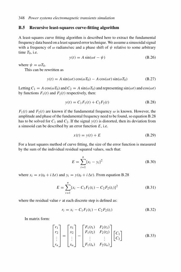
348 Power systems electromagnetic transients simulation
B.5 Recursive least-squares curve-fitting algorithm
A least-squares curve fitting algorithm is described here to extract the fundamentalfrequency data based on a least squared error technique. We assume a sinusoidal signalwith a frequency of ω radians/sec and a phase shift of ψ relative to some arbitrarytime T0, i.e.
y(t) = A sin(ωt − ψ) (B.26)
where ψ = ωT0.This can be rewritten as
y(t) = A sin(ωt) cos(ωT0) − A cos(ωt) sin(ωT0) (B.27)
Letting C1 = A cos(ωT0) and C2 = A sin(ωT0) and representing sin(ωt) and cos(ωt)
by functions F1(t) and F2(t) respectively, then:
y(t) = C1F1(t) + C2F2(t) (B.28)
F1(t) and F2(t) are known if the fundamental frequency ω is known. However, theamplitude and phase of the fundamental frequency need to be found, so equation B.28has to be solved for C1 and C2. If the signal y(t) is distorted, then its deviation froma sinusoid can be described by an error function E, i.e.
x(t) = y(t) + E (B.29)
For a least squares method of curve fitting, the size of the error function is measuredby the sum of the individual residual squared values, such that:
E =n∑
i=1
{xi − yi}2 (B.30)
where xi = x(t0 + i�t) and yi = y(t0 + i�t). From equation B.28
E =n∑
i=1
{xi − C1F1(ti) − C2F2(ti)}2 (B.31)
where the residual value r at each discrete step is defined as:
ri = xi − C1F1(ti) − C2F2(ti) (B.32)
In matrix form:⎡
⎢⎢⎢⎣
r1r2...
rn
⎤
⎥⎥⎥⎦
=
⎡
⎢⎢⎢⎣
x1x2...
xn
⎤
⎥⎥⎥⎦
−
⎡
⎢⎢⎢⎣
F1(t1) F2(t1)
F1(t2) F2(t2)...
...
F1(tn) F2(tn)
⎤
⎥⎥⎥⎦
[C1C2
](B.33)
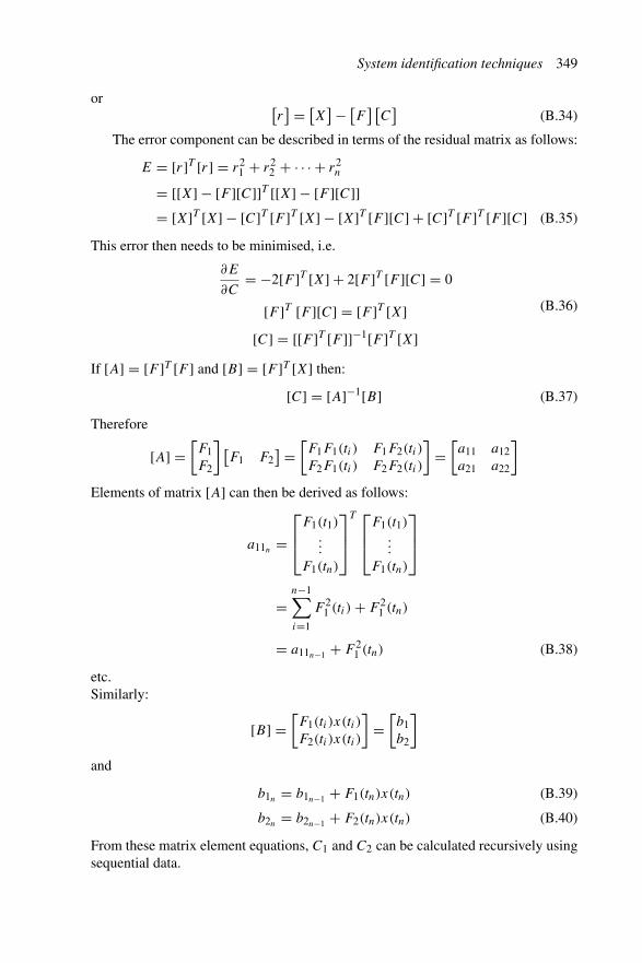
System identification techniques 349
or [r] = [
X] − [
F] [
C]
(B.34)
The error component can be described in terms of the residual matrix as follows:
E = [r]T [r] = r21 + r2
2 + · · · + r2n
= [[X] − [F ][C]]T [[X] − [F ][C]]= [X]T [X] − [C]T [F ]T [X] − [X]T [F ][C] + [C]T [F ]T [F ][C] (B.35)
This error then needs to be minimised, i.e.
∂E
∂C= −2[F ]T [X] + 2[F ]T [F ][C] = 0
[F ]T [F ][C] = [F ]T [X][C] = [[F ]T [F ]]−1[F ]T [X]
(B.36)
If [A] = [F ]T [F ] and [B] = [F ]T [X] then:
[C] = [A]−1[B] (B.37)
Therefore
[A] =[F1F2
] [F1 F2
] =[F1F1(ti) F1F2(ti)
F2F1(ti) F2F2(ti)
]=
[a11 a12a21 a22
]
Elements of matrix [A] can then be derived as follows:
a11n =⎡
⎢⎣
F1(t1)...
F1(tn)
⎤
⎥⎦
T ⎡
⎢⎣
F1(t1)...
F1(tn)
⎤
⎥⎦
=n−1∑
i=1
F 21 (ti) + F 2
1 (tn)
= a11n−1 + F 21 (tn) (B.38)
etc.Similarly:
[B] =[F1(ti)x(ti)
F2(ti)x(ti)
]=
[b1b2
]
and
b1n = b1n−1 + F1(tn)x(tn) (B.39)
b2n = b2n−1 + F2(tn)x(tn) (B.40)
From these matrix element equations, C1 and C2 can be calculated recursively usingsequential data.

350 Power systems electromagnetic transients simulation
B.6 References
1 ABUR, A. and SINGH, H.: ‘Time domain modeling of external systems for elec-tromagnetic transients programs’, IEEE Transactions on Power Systems, 1993,8 (2), pp. 671–77
2 PARK, T. W. and BURRUS, C. S.: ‘Digital filter design’ (John Wiley Interscience,New York, 1987)
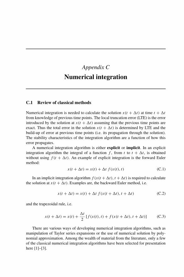
Appendix C
Numerical integration
C.1 Review of classical methods
Numerical integration is needed to calculate the solution x(t + �t) at time t + �t
from knowledge of previous time points. The local truncation error (LTE) is the errorintroduced by the solution at x(t + �t) assuming that the previous time points areexact. Thus the total error in the solution x(t + �t) is determined by LTE and thebuild-up of error at previous time points (i.e. its propagation through the solution).The stability characteristics of the integration algorithm are a function of how thiserror propagates.
A numerical integration algorithm is either explicit or implicit. In an explicitintegration algorithm the integral of a function f , from t to t + �t , is obtainedwithout using f (t + �t). An example of explicit integration is the forward Eulermethod:
x(t + �t) = x(t) + �t f (x(t), t) (C.1)
In an implicit integration algorithm f (x(t + �t), t + �t) is required to calculatethe solution at x(t + �t). Examples are, the backward Euler method, i.e.
x(t + �t) = x(t) + �t f (x(t + �t), t + �t) (C.2)
and the trapezoidal rule, i.e.
x(t + �t) = x(t) + �t
2[f (x(t), t) + f (x(t + �t), t + �t)] (C.3)
There are various ways of developing numerical integration algorithms, such asmanipulation of Taylor series expansions or the use of numerical solution by poly-nomial approximation. Among the wealth of material from the literature, only a fewof the classical numerical integration algorithms have been selected for presentationhere [1]–[3].
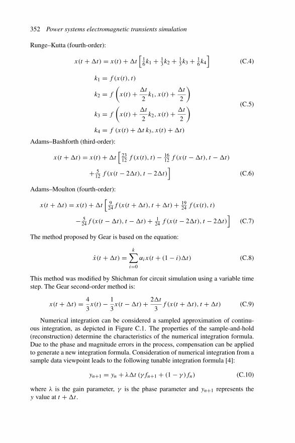
352 Power systems electromagnetic transients simulation
Runge–Kutta (fourth-order):
x(t + �t) = x(t) + �t[
16k1 + 1
3k2 + 13k3 + 1
6k4
](C.4)
k1 = f (x(t), t)
k2 = f
(x(t) + �t
2k1, x(t) + �t
2
)
k3 = f
(x(t) + �t
2k2, x(t) + �t
2
)
k4 = f (x(t) + �t k3, x(t) + �t)
(C.5)
Adams–Bashforth (third-order):
x(t + �t) = x(t) + �t[
2312 f (x(t), t) − 16
12 f (x(t − �t), t − �t)
+ 512 f (x(t − 2�t), t − 2�t)
](C.6)
Adams–Moulton (fourth-order):
x(t + �t) = x(t) + �t[
924f (x(t + �t), t + �t) + 19
24 f (x(t), t)
− 524f (x(t − �t), t − �t) + 1
24 f (x(t − 2�t), t − 2�t)]
(C.7)
The method proposed by Gear is based on the equation:
x(t + �t) =k∑
i=0
αix(t + (1 − i)�t) (C.8)
This method was modified by Shichman for circuit simulation using a variable timestep. The Gear second-order method is:
x(t + �t) = 4
3x(t) − 1
3x(t − �t) + 2�t
3f (x(t + �t), t + �t) (C.9)
Numerical integration can be considered a sampled approximation of continu-ous integration, as depicted in Figure C.1. The properties of the sample-and-hold(reconstruction) determine the characteristics of the numerical integration formula.Due to the phase and magnitude errors in the process, compensation can be appliedto generate a new integration formula. Consideration of numerical integration from asample data viewpoint leads to the following tunable integration formula [4]:
yn+1 = yn + λ�t (γfn+1 + (1 − γ )fn) (C.10)
where λ is the gain parameter, γ is the phase parameter and yn+1 represents they value at t + �t .

Numerical integration 353
s
1
s
Zero-orderhold
1
s
Continuous
Discrete approximation
x (s)
x (s)
x�(Z ) x�(S ) x�(S ) x�(Z )
1 – e–sΔt
.
x (s) x (s).
x�(t).
x�(t + �Δt) x�(t + �Δt) x�(nΔt + �Δt).
...
x (nΔt).
Sample Reconstruction Compensation SampleIntegration
�e� sΔt
Figure C.1 Numerical integration from the sampled data viewpoint
Table C.1 Classical integration formulae as special cases of thetunable integrator
γ Integration Rule Formula
0 Forward Euler yn+1 = yn + �tfn
1
2Trapezoidal yn+1 = yn + �t
2
(fn+1 + fn
)
1 Backward Euler yn+1 = yn + �tfn+13
2Adams–Bashforth 2nd order yn+1 = yn + �t
2
(3fn+1 − fn
)
Tunable yn+1 = yn + λ�t(γfn+1 + (1 − γ )fn
)
If λ = 1 and γ = (1 + α)/2 then the trapezoidal rule with damping is obtained[5]. The selection of integer multiples of half for the phase parameter produces theclassical integration formulae shown in Table C.1. These formulae are actually thesame integrator, differing only in the amount of phase shift of the integrand.
With respect to the differential equation:
yn+1 = f (y, t) (C.11)
Table C.2 shows the various integration rules in the form of an integrator anddifferentiator.
Using numerical integration substitution for the differential equations of an induc-tor and a capacitor gives the Norton equivalent values shown in Tables C.3 and C.4respectively.
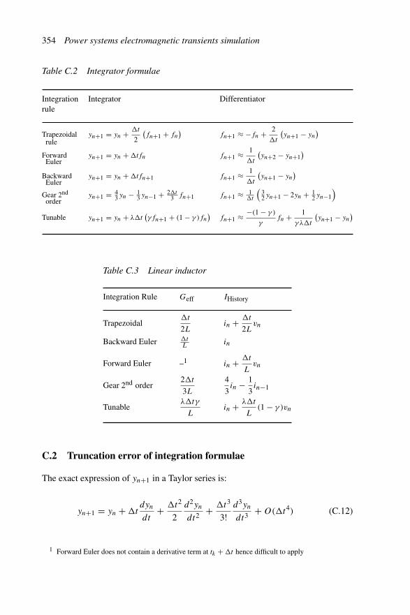
354 Power systems electromagnetic transients simulation
Table C.2 Integrator formulae
Integrationrule
Integrator Differentiator
Trapezoidalrule
yn+1 = yn + �t
2
(fn+1 + fn
)fn+1 ≈ −fn + 2
�t
(yn+1 − yn
)
ForwardEuler
yn+1 = yn + �tfn fn+1 ≈ 1
�t
(yn+2 − yn+1
)
BackwardEuler
yn+1 = yn + �tfn+1 fn+1 ≈ 1
�t
(yn+1 − yn
)
Gear 2nd
orderyn+1 = 4
3 yn − 13 yn−1 + 2�t
3 fn+1 fn+1 ≈ 1�t
(32 yn+1 − 2yn + 1
2 yn−1
)
Tunable yn+1 = yn + λ�t(γfn+1 + (1 − γ )fn
)fn+1 ≈ −(1 − γ )
γfn + 1
γ λ�t
(yn+1 − yn
)
Table C.3 Linear inductor
Integration Rule Geff IHistory
Trapezoidal�t
2Lin + �t
2Lvn
Backward Euler �tL
in
Forward Euler –1 in + �t
Lvn
Gear 2nd order2�t
3L
4
3in − 1
3in−1
Tunableλ�tγ
Lin + λ�t
L(1 − γ )vn
C.2 Truncation error of integration formulae
The exact expression of yn+1 in a Taylor series is:
yn+1 = yn + �tdyn
dt+ �t2
2
d2yn
dt2+ �t3
3!d3yn
dt3+ O(�t4) (C.12)
1 Forward Euler does not contain a derivative term at tk + �t hence difficult to apply
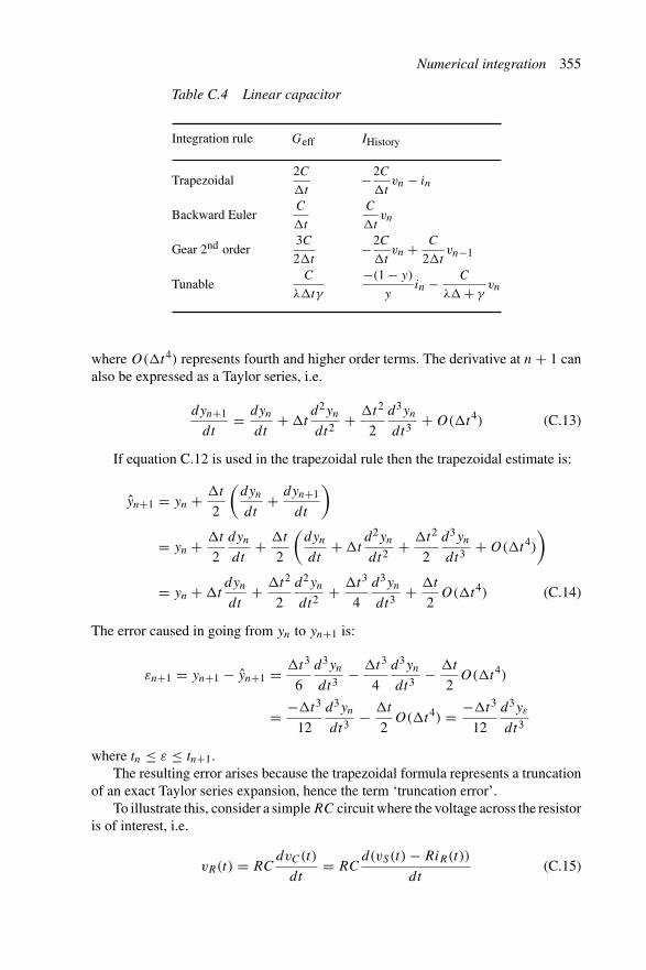
Numerical integration 355
Table C.4 Linear capacitor
Integration rule Geff IHistory
Trapezoidal2C
�t−2C
�tvn − in
Backward EulerC
�t
C
�tvn
Gear 2nd order3C
2�t−2C
�tvn + C
2�tvn−1
TunableC
λ�tγ
−(1 − y)
yin − C
λ� + γvn
where O(�t4) represents fourth and higher order terms. The derivative at n + 1 canalso be expressed as a Taylor series, i.e.
dyn+1
dt= dyn
dt+ �t
d2yn
dt2+ �t2
2
d3yn
dt3+ O(�t4) (C.13)
If equation C.12 is used in the trapezoidal rule then the trapezoidal estimate is:
yn+1 = yn + �t
2
(dyn
dt+ dyn+1
dt
)
= yn + �t
2
dyn
dt+ �t
2
(dyn
dt+ �t
d2yn
dt2+ �t2
2
d3yn
dt3+ O(�t4)
)
= yn + �tdyn
dt+ �t2
2
d2yn
dt2+ �t3
4
d3yn
dt3+ �t
2O(�t4) (C.14)
The error caused in going from yn to yn+1 is:
εn+1 = yn+1 − yn+1 = �t3
6
d3yn
dt3− �t3
4
d3yn
dt3− �t
2O(�t4)
= −�t3
12
d3yn
dt3− �t
2O(�t4) = −�t3
12
d3yε
dt3
where tn ≤ ε ≤ tn+1.The resulting error arises because the trapezoidal formula represents a truncation
of an exact Taylor series expansion, hence the term ‘truncation error’.To illustrate this, consider a simple RC circuit where the voltage across the resistor
is of interest, i.e.
vR(t) = RCdvC(t)
dt= RC
d(vS(t) − RiR(t))
dt(C.15)

356 Power systems electromagnetic transients simulation
Table C.5 Comparison of numerical integration algorithms(�T = τ/10)
Step Exact F. Euler B. Euler Trapezoidal Gear second-order
1 45.2419 45.0000 45.4545 45.2381 –2 40.9365 40.5000 41.3223 40.9297 40.92733 37.0409 36.4500 37.5657 37.0316 37.02114 33.5160 32.8050 34.1507 33.5048 33.48665 30.3265 29.5245 31.0461 30.3139 30.2891
Table C.6 Comparison of numerical integration algorithms (�T = τ )
Step Exact F. Euler B. Euler Trapezoidal Gear second-order
1 18.3940 0.0000 25.0000 16.6667 18.39402 6.7668 0.0000 12.5000 5.5556 4.71523 2.4894 0.0000 6.2500 1.8519 0.09334 0.9158 0.0000 3.1250 0.6173 −0.86845 0.3369 0.0000 1.5625 0.2058 −0.7134
If the applied voltage is a step function at t = 0 then dvS(t)/dt = 0 and equation C.15becomes:
vR(t) = RCdvR(t)
dt= τ
dvR(t)
dt(C.16)
The results for step lengths of τ/10 and τ (vs = 50 V) are shown in Tables C.5 and C.6respectively. Gear second-order is a two-step method and hence the value at �T isrequired as initial condition.
For the trapezoidal rule the ratio (1 − �t/(2τ))/ (1 + �t/(2τ)) remains less than1, so that the solution does tend to zero for any time step size. However for �t > 2τ
it does so in an oscillatory manner and convergence may be very slow.
C.3 Stability of integration methods
Truncation error is a localised property (i.e. local to the present time point and timestep) whereas stability is a global property related to the growth or decay of errorsintroduced at each time point and propagated to successive time points. Stabilitydepends on both the method and the problem.
Since general stability analysis is difficult the normal approach is to compare thestability of different methods for a single test equation, such as:
y = f (y, t) = λy (C.17)
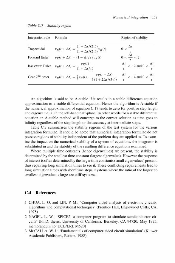
Numerical integration 357
Table C.7 Stability region
Integration rule Formula Region of stability
Trapezoidal vR(t + �t) = (1 − �t/(2τ))
(1 + �t/(2τ))vR(t) 0 <
�t
τ
Forward Euler vR(t + �t) = (1 − �t/τ) vR(t) 0 <�t
τ< 2
Backward Euler vR(t + �t) = vR(t)
(1 + �t/τ)
�t
τ< −2 and 0 <
�t
τ
Gear 2nd order vR(t + �t) = 43vR(t) − vR(t − �t)
3 (1 + 2�t/(3τ))
�t
τ< −4 and 0 <
�t
τ
An algorithm is said to be A-stable if it results in a stable difference equationapproximation to a stable differential equation. Hence the algorithm is A-stable ifthe numerical approximation of equation C.17 tends to zero for positive step lengthand eigenvalue, λ, in the left-hand half-plane. In other words for a stable differentialequation an A-stable method will converge to the correct solution as time goes toinfinity regardless of the step length or the accuracy at intermediate steps.
Table C.7 summarises the stability regions of the test system for the variousintegration formulae. It should be noted that numerical integration formulae do notpossess regions of stability independent of the problem they are applied to. To exam-ine the impact on the numerical stability of a system of equations, the integrator issubstituted in and the stability of the resulting difference equations examined.
Where multiple time constants (hence eigenvalues) are present, the stability isdetermined by the smallest time constant (largest eigenvalue). However the responseof interest is often determined by the larger time constants (small eigenvalues) present,thus requiring long simulation times to see it. These conflicting requirements lead tolong simulation times with short time steps. Systems where the ratio of the largest tosmallest eigenvalue is large are stiff systems.
C.4 References
1 CHUA, L. O. and LIN, P. M.: ‘Computer aided analysis of electronic circuits:algorithms and computational techniques’ (Prentice Hall, Englewood Cliffs, CA,1975)
2 NAGEL, L. W.: ‘SPICE2: a computer program to simulate semiconductor cir-cuits’ (Ph.D. thesis, University of California, Berkeley, CA 94720, May 1975,memorandum no. UCB/ERL M520)
3 McCALLA, W. J.: ‘Fundamentals of computer-aided circuit simulation’ (KluwerAcademic Publishers, Boston, 1988)

358 Power systems electromagnetic transients simulation
4 SMITH, J. M.: ‘Mathematical modeling and digital simulation for engineers andscientists’ (John Wiley & Sons, New York, 2nd edition, 1987)
5 ALVARADO, F. L., LASSETER, R. H. and SANCHEZ, J. J.: ‘Testing of trape-zoidal integration with damping for the solution of power transient problems’, IEEETransactions on Power Apparatus and Systems, 1983, 102 (12), pp. 3783–90

Appendix D
Test systems data
D.1 CIGRE HVDC benchmark model
The CIGRE benchmark model [1] consists of weak rectifier and inverter a.c. systemsresonant at the second harmonic and a d.c. system resonant at the fundamental fre-quency. Both a.c. systems are balanced and connected in star-ground. The system isshown in Figure D.1 with additional information in Tables D.1 and D.2. The HVDClink is a 12-pulse monopolar configuration with the converter transformers connectedstar-ground/star and star-ground/delta. Figures D.2–D.4 show the impedance scansof the a.c. and d.c. systems. A phase imbalance is created in the inverter a.c. systemby inserting typically a 5.0 per cent resistance into one phase in series with the a.c.system.
D.2 Lower South Island (New Zealand) system
The New Zealand Lower South Island power system, shown in Figure D.5, is a usefultest system due to its naturally imbalanced form and to the presence of a large powerconverter situated at the Tiwai-033 busbar. Apart from the converter installation, the
Inverter ac systemRectifier ac system
211.42 : 230 kV345 kV : 211.42 kV
26.0γ = 15α = 15
0.99 pu1.01 pu
0.03650.7406
24.81
116.38
13.230.0606167.2
0.03650.7406
7.522
15.04
0.0061
37.03
15.04a = 1.01 a = 0.989
1 : a
1 : aa : 1
a : 1
2000 A
1.0 pu 1.0 pu 0.935 pu1.088 pu
83.32
0.136
261.87 6.685
6.685
0.59682.5 0.59680.151
2160.63.737
3.342
74.280.136429.76
2.5
Figure D.1 CIGRE HVDC benchmark test system (all components in Ω , H and μF)

360 Power systems electromagnetic transients simulation
Table D.1 CIGRE model main parameters
Parameter Rectifier Inverter
a.c. system voltage 345 kV l–l 230 kV l–la.c. system impedance magnitude 119.03 � 52.9 �
Converter transformer tap (prim. side) 1.01 0.989Equivalent commutation reactance 27 � 27 �
d.c. voltage 505 kV 495 kVd.c. current 2 kA 2 kAFiring angle 15◦ 15◦d.c. power 1010 MW 990 MW
Table D.2 CIGRE model extra information
Rectifier a.c. voltage base 345.0 kVInverter a.c. voltage base 230 kVRectifier voltage source 1.088 � 22.18◦Inverter voltage source 0.935 � −23.14◦Nominal d.c. voltage 500 kVTransformer power base 598 MVATransformer leakage reactance 0.18 puTransformer secondary voltage 211.42 kVNominal rectifier firing angle 15.0◦Nominal inverter extinction angle 15.0◦Thyristor forward voltage drop 0.001 kVThyristor onstate resistance 0.01 �
Snubber resistance 5000 �
Snubber capacitance 0.05 μFd.c. current transducer gain 0.5d.c. current transducer time constant 0.001 sPI controller proportional gain 1.0989PI controller time constant 0.0091 sType-1 filter Shunt capacitorType-2 filter Single tuned filterType-3 filter Special CIGRE filter
system includes two major city loads that vary significantly over the daily period.The 220 kV transmission lines are all specified by their geometry and conductorspecifications, and consequently are unbalanced and coupled between sequences.Tables D.3–D.9 show all of the necessary information.
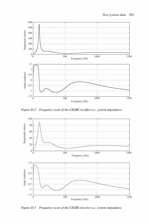
Test systems data 361
Frequency (Hz)
–1.5
–1
–0.5
0
0.5
1
1.5
100
200
300
400
500
600M
agni
tude
(oh
ms)
Ang
le (
radi
ans)
Frequency (Hz)
00 500 1000 1500
0 500 1000 1500
Figure D.2 Frequency scan of the CIGRE rectifier a.c. system impedance
Frequency (Hz)
0
20
40
60
80
100
0 500 1000 1500
–1.5
–1
–0.5
0
0.5
1
1.5
Mag
nitu
de (
ohm
s)A
ngle
(ra
dian
s)
0 500 1000 1500Frequency (Hz)
Figure D.3 Frequency scan of the CIGRE inverter a.c. system impedance

362 Power systems electromagnetic transients simulation
Table D.3 Converter information for the Lower South Islandtest system
Phase shift Xl Vpri. Vsec. Pbase
Converter 1 22.5◦ 0.05 pu 33.0 kV 5.0 kV 100 MVAConverter 2 7.5◦ 0.05 pu 33.0 kV 5.0 kV 100 MVAConverter 3 −7.5◦ 0.05 pu 33.0 kV 5.0 kV 100 MVAConverter 4 −22.5◦ 0.05 pu 33.0 kV 5.0 kV 100 MVA
Table D.4 Transmission line parameters for Lower South Island test system
Busbars Length Conductor type Earth-wire type
Manapouri-220 to Invercargill-220 152.90 km GOAT (30/3.71 + 7/3.71 ACSR) (7/3.05 Gehss)Manapouri-220 to Tiwai-220 175.60 km GOAT (30/3.71 + 7/3.71 ACSR) (7/3.05 Gehss)Invercargill-220 to Tiwai-220 24.30 km GOAT (30/3.71 + 7/3.71 ACSR) (7/3.05 Gehss)Invercargill-220 to Roxburgh-220 129.80 km ZEBRA (54/3.18 + 7/3.18 ACSR) (7/3.05 Gehss)Invercargill-220 to Roxburgh-220 132.20 km ZEBRA (54/3.18 + 7/3.18 ACSR) –
Mag
nitu
de (
ohm
s)A
ngle
(ra
dian
s)
1000
2000
3000
4000
5000
6000
00 50 100 150 200 250 300 350 400 450 500
–2
–1
0
1
2
0 50 100 150 200 250 300 350 400 450 500
Frequency (Hz)
Frequency (Hz)
Figure D.4 Frequency scan of the CIGRE d.c. system impedance
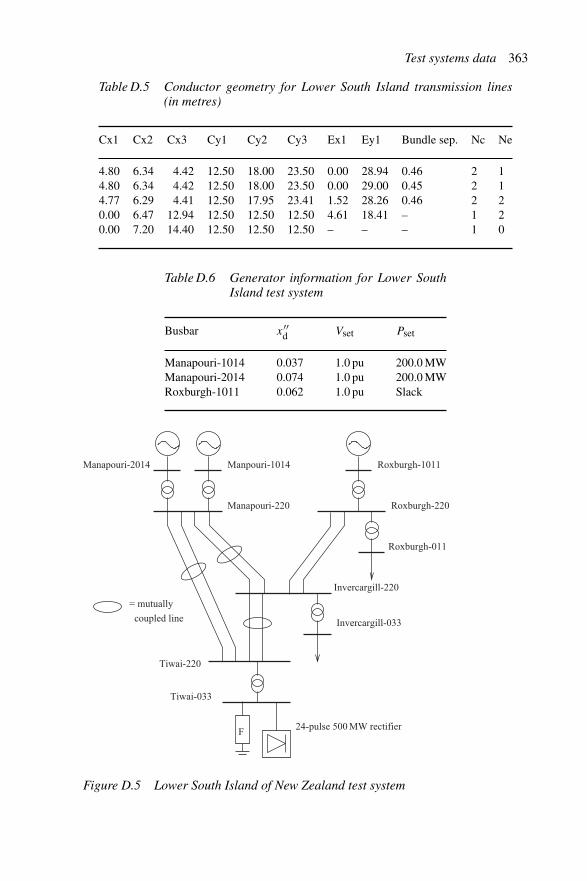
Test systems data 363
Table D.5 Conductor geometry for Lower South Island transmission lines(in metres)
Cx1 Cx2 Cx3 Cy1 Cy2 Cy3 Ex1 Ey1 Bundle sep. Nc Ne
4.80 6.34 4.42 12.50 18.00 23.50 0.00 28.94 0.46 2 14.80 6.34 4.42 12.50 18.00 23.50 0.00 29.00 0.45 2 14.77 6.29 4.41 12.50 17.95 23.41 1.52 28.26 0.46 2 20.00 6.47 12.94 12.50 12.50 12.50 4.61 18.41 – 1 20.00 7.20 14.40 12.50 12.50 12.50 – – – 1 0
Table D.6 Generator information for Lower SouthIsland test system
Busbar x′′d Vset Pset
Manapouri-1014 0.037 1.0 pu 200.0 MWManapouri-2014 0.074 1.0 pu 200.0 MWRoxburgh-1011 0.062 1.0 pu Slack
F
Manapouri-220
Manpouri-1014 Roxburgh-1011
Roxburgh-220
Roxburgh-011
Invercargill-220
Manapouri-2014
= mutually
coupled line
Tiwai-220
Tiwai-033
24-pulse 500 MW rectifier
Invercargill-033
Figure D.5 Lower South Island of New Zealand test system
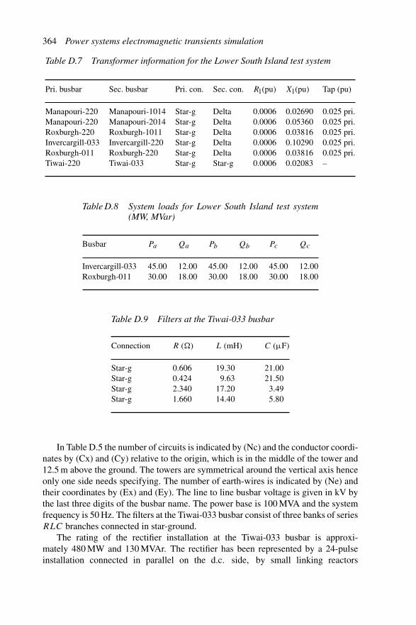
364 Power systems electromagnetic transients simulation
Table D.7 Transformer information for the Lower South Island test system
Pri. busbar Sec. busbar Pri. con. Sec. con. Rl(pu) Xl(pu) Tap (pu)
Manapouri-220 Manapouri-1014 Star-g Delta 0.0006 0.02690 0.025 pri.Manapouri-220 Manapouri-2014 Star-g Delta 0.0006 0.05360 0.025 pri.Roxburgh-220 Roxburgh-1011 Star-g Delta 0.0006 0.03816 0.025 pri.Invercargill-033 Invercargill-220 Star-g Delta 0.0006 0.10290 0.025 pri.Roxburgh-011 Roxburgh-220 Star-g Delta 0.0006 0.03816 0.025 pri.Tiwai-220 Tiwai-033 Star-g Star-g 0.0006 0.02083 –
Table D.8 System loads for Lower South Island test system(MW, MVar)
Busbar Pa Qa Pb Qb Pc Qc
Invercargill-033 45.00 12.00 45.00 12.00 45.00 12.00Roxburgh-011 30.00 18.00 30.00 18.00 30.00 18.00
Table D.9 Filters at the Tiwai-033 busbar
Connection R (�) L (mH) C (μF)
Star-g 0.606 19.30 21.00Star-g 0.424 9.63 21.50Star-g 2.340 17.20 3.49Star-g 1.660 14.40 5.80
In Table D.5 the number of circuits is indicated by (Nc) and the conductor coordi-nates by (Cx) and (Cy) relative to the origin, which is in the middle of the tower and12.5 m above the ground. The towers are symmetrical around the vertical axis henceonly one side needs specifying. The number of earth-wires is indicated by (Ne) andtheir coordinates by (Ex) and (Ey). The line to line busbar voltage is given in kV bythe last three digits of the busbar name. The power base is 100 MVA and the systemfrequency is 50 Hz. The filters at the Tiwai-033 busbar consist of three banks of seriesRLC branches connected in star-ground.
The rating of the rectifier installation at the Tiwai-033 busbar is approxi-mately 480 MW and 130 MVAr. The rectifier has been represented by a 24-pulseinstallation connected in parallel on the d.c. side, by small linking reactors

Test systems data 365
(R = 1 μΩ, L = 1 μH) to an ideal current source (80 kA). The converters are dioderectifiers and the transformer specifications are given in Table D.3.
D.3 Reference
1 SZECHTMAN, M., WESS, T. and THIO, C.V.: ‘First benchmark model for HVdccontrol studies’, ELECTRA, 1991, 135, pp. 55–75

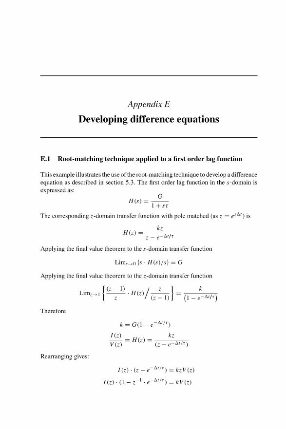
Appendix E
Developing difference equations
E.1 Root-matching technique applied to a first order lag function
This example illustrates the use of the root-matching technique to develop a differenceequation as described in section 5.3. The first order lag function in the s-domain isexpressed as:
H(s) = G
1 + sτ
The corresponding z-domain transfer function with pole matched (as z = es�t ) is
H(z) = kz
z − e−�t/τ
Applying the final value theorem to the s-domain transfer function
Lims→0 {s · H(s)/s} = G
Applying the final value theorem to the z-domain transfer function
Limz→1
{(z − 1)
z· H(z)
/ z
(z − 1)
}= k
(1 − e−�t/τ
)
Therefore
k = G(1 − e−�t/τ )
I (z)
V (z)= H(z) = kz
(z − e−�t/τ )
Rearranging gives:
I (z) · (z − e−�t/τ ) = kzV (z)
I (z) · (1 − z−1 · e−�t/τ ) = kV (z)

368 Power systems electromagnetic transients simulation
HenceI (z) = kV (z) + e−�t/τ z−1I (z)
or in the time domain the exponential form of difference equation becomes:
i(t) = G(1 − e−�t/τ ) · v(t) + e−�t/τ i(t − �t) (E.1)
E.2 Root-matching technique applied to a first orderdifferential pole function
This example illustrates the use of the root-matching technique to develop a differenceequation as described in section 5.3, for a first order differential pole function. Thes-domain expression for the first order differential pole function is:
H(s) = Gs
1 + sτ
The z-domain transfer function with pole and zero matched (using z = es�t ) is
H(z) = k(z − 1)
z − e−�t/τ
Applying the final value theorem to the s-domain transfer function for a unit rampinput:
Lims→0
{s · H(s)/s2
}= G
Applying the final value theorem to the z-domain transfer function:
Limz→0
{(z − 1)
z· H(z)
/ z�t
(z − 1)2
}= k�t
(1 − e−�t/τ
)
Therefore
k = G(1 − e−�t/τ )/�t
I (z)
V (z)= H(z) = k (z − 1)
(z − e−�t/τ )
Rearranging gives:
I (z)(z − e−�t/τ ) = k (z − 1) V (z)
I (z)(1 − z−1 · e−�t/τ ) = k(1 − z−1)V (z)
HenceI (z) = kV (z) − k · z−1V (z) + e−�t/τ z−1I (z)

Developing difference equations 369
E.3 Difference equation by bilinear transformationfor RL series branch
For comparison the bilinear transform is applied to the s-domain rational function fora series RL branch
Y (s) = I (s)
V (s)= 1
R + sL
Applying the bilinear transformation (s ≈ 2(1 − z−1)/(�t(1 + z−1)):
Y (z) = 1
R + 2L(1 − z−1)/(�t(1 + z−1))
= (1 + z−1)
(R + 2L/�t) + z−1 · (R − 2L/�t)
= (1 + z−1)/(R + 2L/�t)
1 + z−1 · (R − 2L/�t)/(R + 2L/�t)(E.2)
E.4 Difference equation by numerical integrator substitutionfor RL series branch
Next numerical integrator substitution is applied to a series RL branch, to show thatit does give the same difference equation as using the bilinear transform
di
dt= 1
L(v − R · i)
Hence
ik = ik−1 +∫ t
t−�t
di
dtdt
Applying the trapezoidal rule gives:
ik = ik−1 + �t
2
(dik
dt+ dik−1
dt
)
Substituting in the branch equation yields:
di
dt= 1
L(v − R · i)
ik = ik−1 +∫ t
t−�t
di
ik = ik−1 + �t
2
(dik
dt+ dik−1
dt
)
ik = ik−1 + �t
2
(1
L(vk − R · ik) + 1
L(vk−1 − R · ik−1)
)
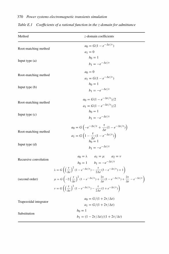
370 Power systems electromagnetic transients simulation
Table E.1 Coefficients of a rational function in the z-domain for admittance
Method z-domain coefficients
Root-matching methoda0 = G(1 − e−�t/τ )
a1 = 0
Input type (a)b0 = 1
b1 = −e−�t/τ
Root-matching methoda0 = 0
a1 = G(1 − e−�t/τ )
Input type (b)b0 = 1
b1 = −e−�t/τ
Root-matching methoda0 = G(1 − e−�t/τ )/2
a1 = G(1 − e−�t/τ )/2
Input type (c)b0 = 1
b1 = −e−�t/τ
Root-matching methoda0 = G
(−e−�t/τ + τ
�t(1 − e−�t/τ )
)
a1 = G(
1 − τ
�t(1 − e−�t/τ )
)
Input type (d)b0 = 1
b1 = −e−�t/τ
Recursive convolutiona0 = λ a1 = μ a2 = ν
b0 = 1 b1 = −e−�t/τ
(second order)
λ = G
(( τ
�t
)2(1 − e−�t/τ ) − τ
2�t(3 − e−�t/τ ) + 1
)
μ = G
(−2
( τ
�t
)2(1 − e−�t/τ ) + 2τ
�t(1 − e−�t/τ ) + 2τ
�t− e−�t/τ
)
ν = G
(( τ
�t
)2(1 − e−�t/τ ) − τ
2�t(1 + e−�t/τ )
)
Trapezoidal integratora0 = G/(1 + 2τ/�t)
a1 = G/(1 + 2τ/�t)
Substitutionb0 = 1
b1 = (1 − 2τ/�t)/(1 + 2τ/�t)

Developing difference equations 371
Table E.2 Coefficients of a rational function in the z-domain for impedance
Method z-domain coefficients
Root-matching methoda0 = 1/G(1 − e−�t/τ )
a1 = −e−�t/τ /G(1 − e−�t/τ )
Input type (a) b0 = 1 b1 = 0
Root-matching methoda0 = 1/G(1 − e−�t/τ )
a1 = −e−�t/τ /G(1 − e−�t/τ )
Input type (b) b0 = 0 b1 = 1
Root-matching methoda0 = 2/G(1 − e−�t/τ )
a1 = −2e−�t/τ /G(1 − e−�t/τ )
Input type (c) b0 = 1 b1 = 1
Root-matching methoda0 = 1/G
(1 − τ
�t(1 − e−�t/τ )
)
a1 = −e−�t/τ /G(
1 − τ
�t(1 − e−�t/τ )
)
Input type (d)b0 = 1
b1 =(−e−�t/τ + τ
�t(1 − e−�t/τ )
)/(1 − τ
�t(1 − e−�t/τ )
)
Recursive convolutiona0 = 1/λ a1 = −e−�t/τ /λ
b0 = 1 b1 = μ/λ b2 = ν/λ
(second order)
λ = G
(( τ
�t
)2(1 − e−�t/τ ) − τ
2�t(3 − e−�t/τ ) + 1
)
μ = G
(−2
( τ
�t
)2(1 − e−�t/τ ) + 2τ
�t(1 − e−�t/τ ) + 2τ
�t− e−�t/τ
)
ν = G
(( τ
�t
)2(1 − e−�t/τ ) − τ
2�t(1 + e−�t/τ )
)
Trapezoidal integrator
a0 = (1 + 2τ/�t)/G
a1 = (1 − 2τ/�t)/G
Substitution b0 = 1 b1 = 1
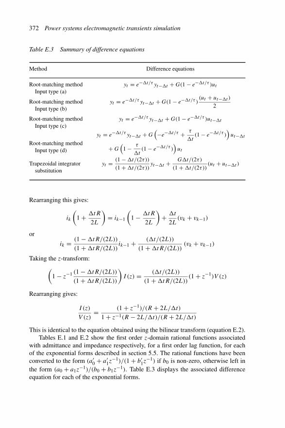
372 Power systems electromagnetic transients simulation
Table E.3 Summary of difference equations
Method Difference equations
Root-matching methodInput type (a)
yt = e−�t/τ yt−�t + G(1 − e−�t/τ )ut
Root-matching methodInput type (b)
yt = e−�t/τ yt−�t + G(1 − e−�t/τ )(ut + ut−�t )
2
Root-matching methodInput type (c)
yt = e−�t/τ yt−�t + G(1 − e−�t/τ )ut−�t
Root-matching methodInput type (d)
yt = e−�t/τ yt−�t + G(−e−�t/τ + τ
�t(1 − e−�t/τ )
)ut−�t
+ G(
1 − τ
�t(1 − e−�t/τ )
)ut
Trapezoidal integratorsubstitution
yt = (1 − �t/(2τ))
(1 + �t/(2τ))yt−�t + G�t/(2τ)
(1 + �t/(2τ))(ut + ut−�t )
Rearranging this gives:
ik
(1 + �tR
2L
)= ik−1
(1 − �tR
2L
)+ �t
2L(vk + vk−1)
or
ik = (1 − �tR/(2L))
(1 + �tR/(2L))ik−1 + (�t/(2L))
(1 + �tR/(2L))(vk + vk−1)
Taking the z-transform:(
1 − z−1 (1 − �tR/(2L))
(1 + �tR/(2L))
)I (z) = (�t/(2L))
(1 + �tR/(2L))(1 + z−1)V (z)
Rearranging gives:
I (z)
V (z)= (1 + z−1)/(R + 2L/�t)
1 + z−1(R − 2L/�t)/(R + 2L/�t)
This is identical to the equation obtained using the bilinear transform (equation E.2).Tables E.1 and E.2 show the first order z-domain rational functions associated
with admittance and impedance respectively, for a first order lag function, for eachof the exponential forms described in section 5.5. The rational functions have beenconverted to the form (a′
0 + a′1z
−1)/(1 + b′1z
−1) if b0 is non-zero, otherwise left inthe form (a0 + a1z
−1)/(b0 + b1z−1). Table E.3 displays the associated difference
equation for each of the exponential forms.
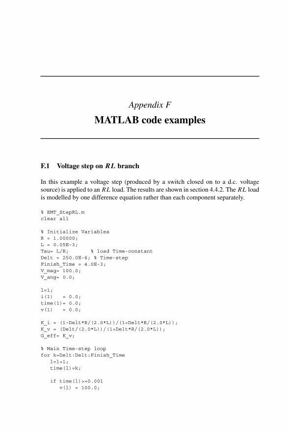
Appendix F
MATLAB code examples
F.1 Voltage step on RL branch
In this example a voltage step (produced by a switch closed on to a d.c. voltagesource) is applied to an RL load. The results are shown in section 4.4.2. The RL loadis modelled by one difference equation rather than each component separately.
% EMT_StepRL.mclear all
% Initialize VariablesR = 1.00000;L = 0.05E-3;Tau= L/R; % load Time-constantDelt = 250.0E-6; % Time-stepFinish_Time = 4.0E-3;V_mag= 100.0;V_ang= 0.0;
l=1;i(1) = 0.0;time(1)= 0.0;v(1) = 0.0;
K_i = (1-Delt*R/(2.0*L))/(1+Delt*R/(2.0*L));K_v = (Delt/(2.0*L))/(1+Delt*R/(2.0*L));G_eff= K_v;
% Main Time-step loopfor k=Delt:Delt:Finish_Time
l=l+1;time(l)=k;
if time(l)>=0.001v(l) = 100.0;

374 Power systems electromagnetic transients simulation
elsev(l)=0.0;
end;I_history = K_i*i(l-1) + K_v*v(l-1);I_inst = v(l)*G_eff;i(l) = I_inst+I_history;
end;
% Plot resultsfigure(1)plot(time,v,’-k’,time,i,’:k’);legend(’Voltage’,’Current’);xlabel(’Time (Seconds)’);
F.2 Diode fed RL branch
This simple demonstration program is used to show the numerical oscillation thatoccurs at turn-off by modelling an RL load fed from an a.c. source through a diode.The results are shown in section 9.4. The RL load is modelled by one differenceequation rather than each component separately.
% Diode fed RL load% A small demonstration program to demonstrate numerical noise%%%%%%%%%%%%%%%%%%%%%%%%%%%%%%%%%%%%%%%%%%%%%clear all
f =50.0; % Source FrequencyFinish_Time = 60.0E-3;R= 100.0;L= 500.0E-3;Tau= L/R; % Load time-constantDelt = 50.0E-6; % Time-stepV_mag= 230.0*sqrt(2.); % Peak source magnitudeV_ang= 0.0;R_ON = 1.0E-10; % Diode ON ResistanceR_OFF= 1.0E10; % Diode OFF Resistance
% Initial StateON=1;R_switch = R_ON;
l=1;i(1)=0.0;time(1)=0.0;v(1) = V_mag*sin(V_ang*pi/180.0);v_load(1)=v(1);ON = 1;
K_i=(1-Delt*R/(2.0*L))/(1+Delt*R/(2.0*L));K_v=(Delt/(2.0*L))/(1+Delt*R/(2.0*L));G_eff= K_v;G_switch = 1.0/R_switch ;
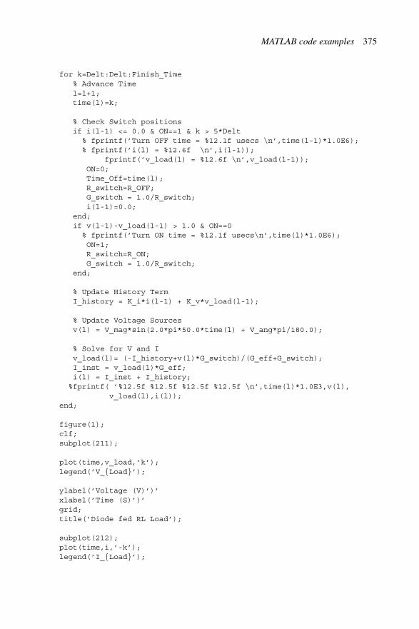
MATLAB code examples 375
for k=Delt:Delt:Finish_Time% Advance Timel=l+1;time(l)=k;
% Check Switch positionsif i(l-1) <= 0.0 & ON==1 & k > 5*Delt
% fprintf(’Turn OFF time = %12.1f usecs \n’,time(l-1)*1.0E6);% fprintf(’i(l) = %12.6f \n’,i(l-1));
fprintf(’v_load(l) = %12.6f \n’,v_load(l-1));ON=0;Time_Off=time(l);R_switch=R_OFF;G_switch = 1.0/R_switch;i(l-1)=0.0;
end;if v(l-1)-v_load(l-1) > 1.0 & ON==0
% fprintf(’Turn ON time = %12.1f usecs\n’,time(l)*1.0E6);ON=1;R_switch=R_ON;G_switch = 1.0/R_switch;
end;
% Update History TermI_history = K_i*i(l-1) + K_v*v_load(l-1);
% Update Voltage Sourcesv(l) = V_mag*sin(2.0*pi*50.0*time(l) + V_ang*pi/180.0);
% Solve for V and Iv_load(l)= (-I_history+v(l)*G_switch)/(G_eff+G_switch);I_inst = v_load(l)*G_eff;i(l) = I_inst + I_history;%fprintf( ’%12.5f %12.5f %12.5f %12.5f \n’,time(l)*1.0E3,v(l),
v_load(l),i(l));end;
figure(1);clf;subplot(211);
plot(time,v_load,’k’);legend(’V_{Load}’);
ylabel(’Voltage (V)’)’xlabel(’Time (S)’)’grid;title(’Diode fed RL Load’);
subplot(212);plot(time,i,’-k’);legend(’I_{Load}’);

376 Power systems electromagnetic transients simulation
ylabel(’Current (A)’)’grid;axis([0.0 0.06 0.0000 2.5])xlabel(’Time (S)’)’
F.3 General version of example F.2
This program models the same case as the program of section F.2, i.e. it shows thenumerical oscillation that occurs at turn-off by modelling an RL load fed from an a.c.source through a diode. However it is now structured in a general manner, where eachcomponent is subject to numerical integrator substitution (NIS) and the conductancematrix is built up. Moreover, rather than modelling the switch as a variable resistor,matrix partitioning is applied (see section 4.4.1), which enables the use of idealswitches.
% General EMT Program%%%%%%%%%%%%%%%%%%%%%%%%%%%%%%%%%%%%%%%%%%%%%clear allglobal Branchglobal No_Brnglobal Sourceglobal No_Sourceglobal No_Nodesglobal i_RLglobal tglobal v_loadglobal v_sglobal V_nglobal V_Kglobal ShowExtra%%%%%%%%%%%%%%%%%%%%%%%%%%%%%%%%%%%%%%%%%%%%%%%%%%%%%%%%%%%% Initialize%%%%%%%%%%%%%%%%%%%%%%%%%%%%%%%%%%%%%%%%%%%%%%%%%%%%%%%%%%%format long
ShowExtra=0;TheTime = 0.0;Finish_Time = 60.0E-3;DeltaT = 50.0E-6;%%%%%%%%%%%%%%%%%%%%%%%%%%%%%%%%%%%%%%%%%%%%%%%%%%%%%%%%%%%% Specify System%%%%%%%%%%%%%%%%%%%%%%%%%%%%%%%%%%%%%%%%%%%%%%%%%%%%%%%%%%%No_Brn=3;No_Nodes=3;No_UnkownNodes=2;No_Source=1;
Branch(1).Type = ’R’;Branch(1).Value= 100.0;Branch(1).Node1= 2;Branch(1).Node2= 1;Branch(1).V_last = 0.0;
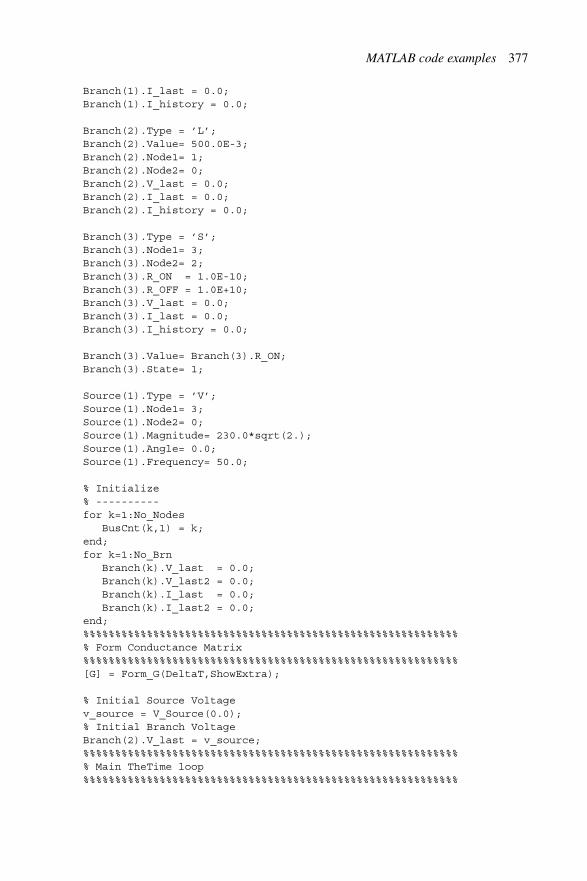
MATLAB code examples 377
Branch(1).I_last = 0.0;Branch(1).I_history = 0.0;
Branch(2).Type = ’L’;Branch(2).Value= 500.0E-3;Branch(2).Node1= 1;Branch(2).Node2= 0;Branch(2).V_last = 0.0;Branch(2).I_last = 0.0;Branch(2).I_history = 0.0;
Branch(3).Type = ’S’;Branch(3).Node1= 3;Branch(3).Node2= 2;Branch(3).R_ON = 1.0E-10;Branch(3).R_OFF = 1.0E+10;Branch(3).V_last = 0.0;Branch(3).I_last = 0.0;Branch(3).I_history = 0.0;
Branch(3).Value= Branch(3).R_ON;Branch(3).State= 1;
Source(1).Type = ’V’;Source(1).Node1= 3;Source(1).Node2= 0;Source(1).Magnitude= 230.0*sqrt(2.);Source(1).Angle= 0.0;Source(1).Frequency= 50.0;
% Initialize% ----------for k=1:No_Nodes
BusCnt(k,1) = k;end;for k=1:No_Brn
Branch(k).V_last = 0.0;Branch(k).V_last2 = 0.0;Branch(k).I_last = 0.0;Branch(k).I_last2 = 0.0;
end;%%%%%%%%%%%%%%%%%%%%%%%%%%%%%%%%%%%%%%%%%%%%%%%%%%%%%%%%%%%% Form Conductance Matrix%%%%%%%%%%%%%%%%%%%%%%%%%%%%%%%%%%%%%%%%%%%%%%%%%%%%%%%%%%%[G] = Form_G(DeltaT,ShowExtra);
% Initial Source Voltagev_source = V_Source(0.0);% Initial Branch VoltageBranch(2).V_last = v_source;%%%%%%%%%%%%%%%%%%%%%%%%%%%%%%%%%%%%%%%%%%%%%%%%%%%%%%%%%%%% Main TheTime loop%%%%%%%%%%%%%%%%%%%%%%%%%%%%%%%%%%%%%%%%%%%%%%%%%%%%%%%%%%%

378 Power systems electromagnetic transients simulation
l = 1;while TheTime <= Finish_Time
%%%%%%%%%%%%%%%%%%%% Advance TheTime %%%%%%%%%%%%%%%%%%%%TheTime = TheTime+DeltaT;l = l+1;t(l) = TheTime;%fprintf(’\n ------------- %12.6f -- l=%d ---------- \n’,TheTime,l);
%%%%%%%%%%%%%%%%%%%%%%%%%%%%% Check Switch positions %%%%%%%%%%%%%%%%%%%%%%%%%%%%%[Reform_G] = Check_Switch(DeltaT,TheTime,v_source,l);if Reform_G == 1
ShowExtra = 0;[G] = Form_G(DeltaT,ShowExtra);
end;%%%%%%%%%%%%%%%%%%%%%%%%%%%%%%%%%%%%%%%%%%%%%% Update Sources%%%%%%%%%%%%%%%%%%%%%%%%%%%%%%%%%%%%%%%%%%%%%v_source = V_Source(TheTime);%%%%%%%%%%%%%%%%%%%%%%%%%%%%%%%%%%%%%%%%%%%%%% Calculate History Terms%%%%%%%%%%%%%%%%%%%%%%%%%%%%%%%%%%%%%%%%%%%%%CalculateBrn_I_history;%%%%%%%%%%%%%%%%%%%%%%%%%%%%%%%%%%%%%%%%%%%%%% Calculate Injection Current Vector%%%%%%%%%%%%%%%%%%%%%%%%%%%%%%%%%%%%%%%%%%%%%[I_history] = Calculate_I_history;%%%%%%%%%%%%%%%%%%%%%%%%%%%%%%%%%%%%%%%%%%%%%%%%%%%%%%%%%%%%%% Partition Conductance Matrix and Injection Current Vector%%%%%%%%%%%%%%%%%%%%%%%%%%%%%%%%%%%%%%%%%%%%%%%%%%%%%%%%%%%%%G_UU = G(1:No_UnkownNodes,1:No_UnkownNodes);G_UK = G(1:No_UnkownNodes,No_UnkownNodes+1:No_Nodes);I_U = I_history(1:No_UnkownNodes)’;% Known Node Voltage% ------------------V_K(1:1) = v_source;%%%%%%%%%%%%%%%%%%%%%%%%%%%%%%%%%%%%%%%%%%%%%% Modified Injection Current Vector%%%%%%%%%%%%%%%%%%%%%%%%%%%%%%%%%%%%%%%%%%%%%I_d_history = I_U - G_UK*V_K;%%%%%%%%%%%%%%%%%%%%%%%%%%%%%%%%%%%%%%%%%%%%%% Solve for Unknown Node Voltages%%%%%%%%%%%%%%%%%%%%%%%%%%%%%%%%%%%%%%%%%%%%%V_U = G_UU\I_d_history;%%%%%%%%%%%%%%%%%%%%%%%%%%%%%%%%%%%%%%%%%%%%%% Rebuild Node Voltage Vector%%%%%%%%%%%%%%%%%%%%%%%%%%%%%%%%%%%%%%%%%%%%%V_n(1:No_UnkownNodes,1) = V_U;V_n(No_UnkownNodes+1:No_Nodes,1)=V_K;%%%%%%%%%%%%%%%%%%%%%%%%%%%%%%%%%%%%%%%%%%%%%
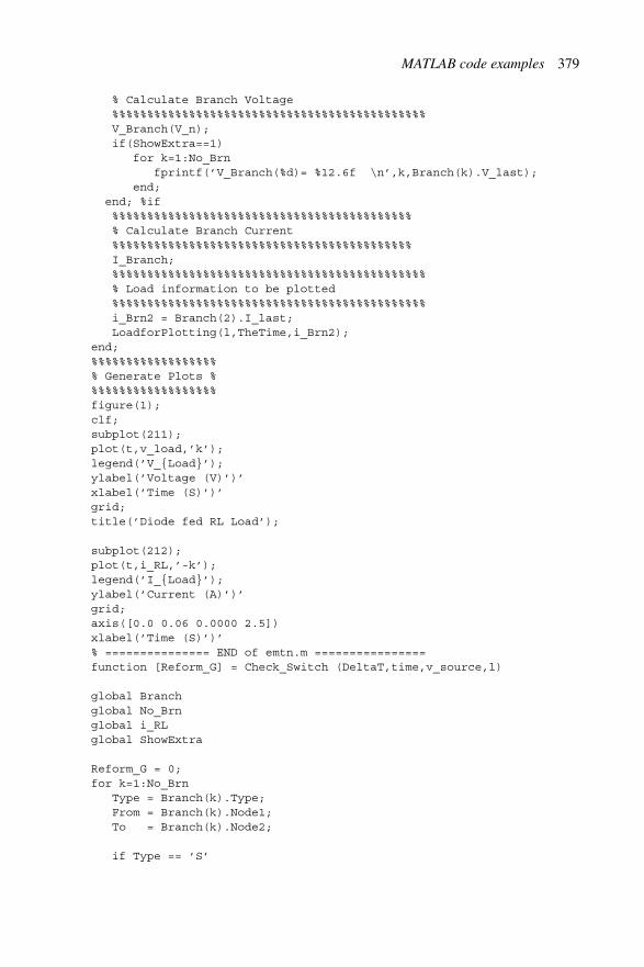
MATLAB code examples 379
% Calculate Branch Voltage%%%%%%%%%%%%%%%%%%%%%%%%%%%%%%%%%%%%%%%%%%%%%V_Branch(V_n);if(ShowExtra==1)
for k=1:No_Brnfprintf(’V_Branch(%d)= %12.6f \n’,k,Branch(k).V_last);
end;end; %if%%%%%%%%%%%%%%%%%%%%%%%%%%%%%%%%%%%%%%%%%%%% Calculate Branch Current%%%%%%%%%%%%%%%%%%%%%%%%%%%%%%%%%%%%%%%%%%%I_Branch;%%%%%%%%%%%%%%%%%%%%%%%%%%%%%%%%%%%%%%%%%%%%%% Load information to be plotted%%%%%%%%%%%%%%%%%%%%%%%%%%%%%%%%%%%%%%%%%%%%%i_Brn2 = Branch(2).I_last;LoadforPlotting(l,TheTime,i_Brn2);
end;%%%%%%%%%%%%%%%%%%% Generate Plots %%%%%%%%%%%%%%%%%%%figure(1);clf;subplot(211);plot(t,v_load,’k’);legend(’V_{Load}’);ylabel(’Voltage (V)’)’xlabel(’Time (S)’)’grid;title(’Diode fed RL Load’);
subplot(212);plot(t,i_RL,’-k’);legend(’I_{Load}’);ylabel(’Current (A)’)’grid;axis([0.0 0.06 0.0000 2.5])xlabel(’Time (S)’)’% =============== END of emtn.m ================function [Reform_G] = Check_Switch (DeltaT,time,v_source,l)
global Branchglobal No_Brnglobal i_RLglobal ShowExtra
Reform_G = 0;for k=1:No_Brn
Type = Branch(k).Type;From = Branch(k).Node1;To = Branch(k).Node2;
if Type == ’S’
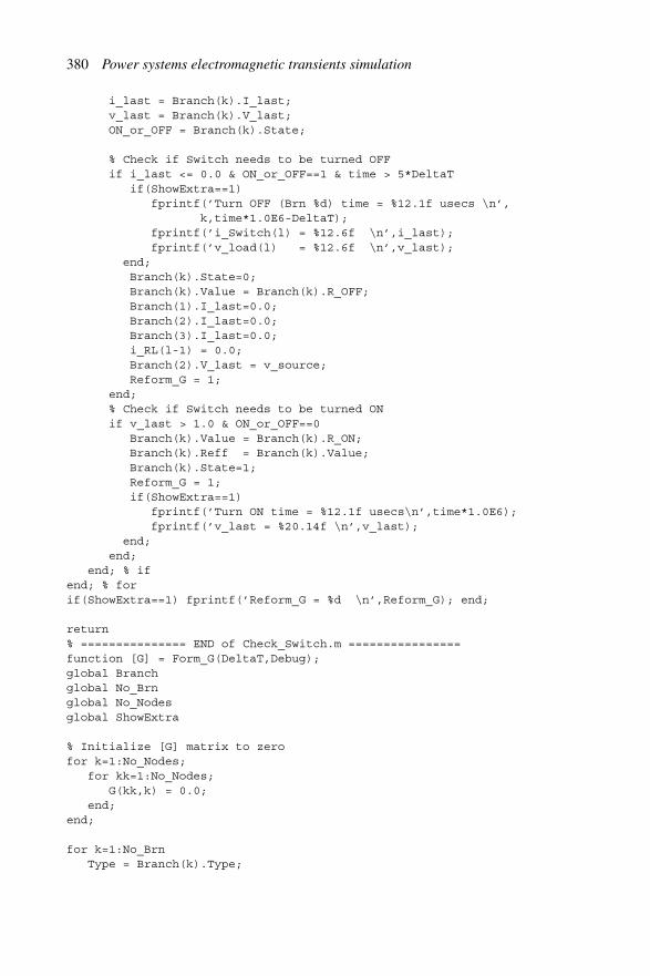
380 Power systems electromagnetic transients simulation
i_last = Branch(k).I_last;v_last = Branch(k).V_last;ON_or_OFF = Branch(k).State;
% Check if Switch needs to be turned OFFif i_last <= 0.0 & ON_or_OFF==1 & time > 5*DeltaT
if(ShowExtra==1)fprintf(’Turn OFF (Brn %d) time = %12.1f usecs \n’,
k,time*1.0E6-DeltaT);fprintf(’i_Switch(l) = %12.6f \n’,i_last);fprintf(’v_load(l) = %12.6f \n’,v_last);
end;Branch(k).State=0;Branch(k).Value = Branch(k).R_OFF;Branch(1).I_last=0.0;Branch(2).I_last=0.0;Branch(3).I_last=0.0;i_RL(l-1) = 0.0;Branch(2).V_last = v_source;Reform_G = 1;
end;% Check if Switch needs to be turned ONif v_last > 1.0 & ON_or_OFF==0
Branch(k).Value = Branch(k).R_ON;Branch(k).Reff = Branch(k).Value;Branch(k).State=1;Reform_G = 1;if(ShowExtra==1)
fprintf(’Turn ON time = %12.1f usecs\n’,time*1.0E6);fprintf(’v_last = %20.14f \n’,v_last);
end;end;
end; % ifend; % forif(ShowExtra==1) fprintf(’Reform_G = %d \n’,Reform_G); end;
return% =============== END of Check_Switch.m ================function [G] = Form_G(DeltaT,Debug);global Branchglobal No_Brnglobal No_Nodesglobal ShowExtra
% Initialize [G] matrix to zerofor k=1:No_Nodes;
for kk=1:No_Nodes;G(kk,k) = 0.0;
end;end;
for k=1:No_BrnType = Branch(k).Type;

MATLAB code examples 381
From = Branch(k).Node1;To = Branch(k).Node2;
Series = 1;if To == 0
To = From;Series = 0;
end;if From == 0
From = To;Series = 0;
end;if To==0
disp(’*** Both Nodes Zero ***’);exit;
end;Branch(k).Series = Series;
if Type == ’R’R_eff = Branch(k).Value;
elseif Type == ’S’R_eff = Branch(k).Value;
elseif Type == ’L’L = Branch(k).Value;R_eff = (2*L)/DeltaT;
elseif Type == ’C’C = Branch(k).Value;R_eff = DeltaT/(2*C);
elsedisp(’*** Invalid Branch Type ***’);exit;
end;Branch(k).Reff = R_eff;
if(ShowExtra==1)fprintf(’Branch %d From %d to %d has Reff= %20.14f Ohms \n’,
k,From,To,R_eff);end;
if Series==1G(To,To) = G(To,To) + 1/R_eff;G(From,From) = G(From,From) + 1/R_eff;G(From,To) = G(From,To) - 1/R_eff;G(To,From) = G(To,From) - 1/R_eff;
elseG(To,To) = G(To,To) + 1/R_eff;
end;end;if(ShowExtra==1)
Gpause;
end;return

382 Power systems electromagnetic transients simulation
% =============== END of Form_G.m ================function [] = CalculateBrn_I_history ()% Calculate Branch History Term%---------------------------------------global Branchglobal No_Brn
for k=1:No_BrnType = Branch(k).Type;if Type == ’R’
Branch(k).I_history =0.0;elseif Type == ’S’
Branch(k).I_history =0.0;elseif Type == ’L’
Branch(k).I_history = Branch(k).I_last + Branch(k).V_last/Branch(k).Reff;elseif Type == ’C’
Branch(k).I_history = -Branch(k).I_last - Branch(k).V_last/Branch(k).Reff;end;
end;
return% =============== END of CalculateBrn_I_history.m ================function [I_History] = Calculate_I_history;% Calculate Current Injection Vector from Branch History Terms% ------------------------------------------------------------global Branchglobal No_Brnglobal No_Nodes
for k=1:No_NodesI_History(k)=0.0;
end;
for k=1:No_BrnType = Branch(k).Type;From = Branch(k).Node1;To = Branch(k).Node2;Brn_I_History = Branch(k).I_history;
if Branch(k).Series==1% Series ComponentI_History(To) = I_History(To) + Brn_I_History;I_History(From) = I_History(From)- Brn_I_History;
elseif To˜= 0
I_History(To) = I_History(To) + Brn_I_History;elseif From˜= 0
I_History(From) = I_History(From)- Brn_I_History;else
disp(’*** Error: Both Nodes Zero ***’);exit;
end;end; %if

MATLAB code examples 383
end; % for% =============== END of Calculate_I_history.m ================function [] = I_Branch;% Calculate Branch Current% ------------------------global Branchglobal No_Brn
for k=1:No_BrnType = Branch(k).Type;From = Branch(k).Node1;To = Branch(k).Node2;V = Branch(k).V_last;
% Save last value to another variable before reassigning last.% Extra Past terms added so Interpolation can be addedBranch(k).I_last3 = Branch(k).I_last2;Branch(k).I_last2 = Branch(k).I_last;
if Type == ’R’Branch(k).I_last = V/Branch(k).Reff;
elseif Type == ’S’Branch(k).I_last = V/Branch(k).Reff;
elseif Type == ’L’Branch(k).I_last = V/Branch(k).Reff + Branch(k).I_history;
elseif Type == ’C’Branch(k).I_last = V/Branch(k).Reff + Branch(k).I_history;
end;end; % forreturn;% =============== END of I_Branch.m ================function [] = V_Branch(V);% Calculates the Branch Voltage% -----------------------------global Branchglobal No_Brn
for k=1:No_BrnFrom = Branch(k).Node1;To = Branch(k).Node2;% Save last value to another variable before reassigning lastBranch(k).V_last3 = Branch(k).V_last2;Branch(k).V_last2 = Branch(k).V_last;
if Branch(k).Series==1% Series ComponentBranch(k).V_last = V(From)-V(To);
elseif To˜= 0
Branch(k).V_last= -V(To);elseif From˜= 0
Branch(k).V_last= V(From);else
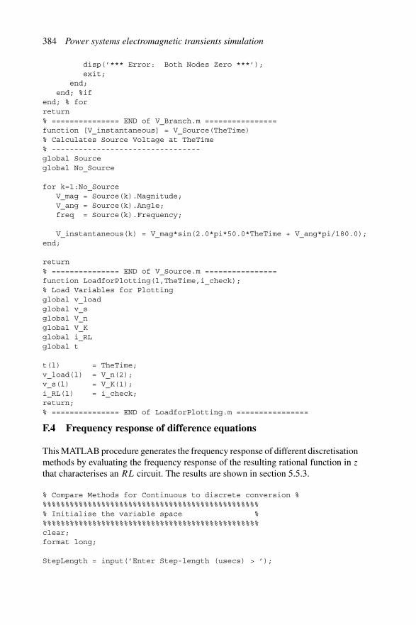
384 Power systems electromagnetic transients simulation
disp(’*** Error: Both Nodes Zero ***’);exit;
end;end; %if
end; % forreturn% =============== END of V_Branch.m ================function [V_instantaneous] = V_Source(TheTime)% Calculates Source Voltage at TheTime% ---------------------------------global Sourceglobal No_Source
for k=1:No_SourceV_mag = Source(k).Magnitude;V_ang = Source(k).Angle;freq = Source(k).Frequency;
V_instantaneous(k) = V_mag*sin(2.0*pi*50.0*TheTime + V_ang*pi/180.0);end;
return% =============== END of V_Source.m ================function LoadforPlotting(l,TheTime,i_check);% Load Variables for Plottingglobal v_loadglobal v_sglobal V_nglobal V_Kglobal i_RLglobal t
t(l) = TheTime;v_load(l) = V_n(2);v_s(l) = V_K(1);i_RL(l) = i_check;return;% =============== END of LoadforPlotting.m ================
F.4 Frequency response of difference equations
This MATLAB procedure generates the frequency response of different discretisationmethods by evaluating the frequency response of the resulting rational function in z
that characterises an RL circuit. The results are shown in section 5.5.3.
% Compare Methods for Continuous to discrete conversion %%%%%%%%%%%%%%%%%%%%%%%%%%%%%%%%%%%%%%%%%%%%%%%%%% Initialise the variable space %%%%%%%%%%%%%%%%%%%%%%%%%%%%%%%%%%%%%%%%%%%%%%%%%clear;format long;
StepLength = input(’Enter Step-length (usecs) > ’);

MATLAB code examples 385
deltaT = StepLength * 1.0E-6;%%%%%%%%%%%%%%%%%%%%%%%%%%%%%%%%%%%%%%%%%%%%%%%%%%%%%%%%%%%%%% Intitalize variables and set up some intermediate results %%%%%%%%%%%%%%%%%%%%%%%%%%%%%%%%%%%%%%%%%%%%%%%%%%%%%%%%%%%%%%
fmax = 1001;R =1.0;L = 50.0E-6;Tau = L/R;G = 1/R;expterm = exp(-deltaT/Tau);Gequ = G*(1.0-exp(-deltaT/Tau));
%% Recursive Convolutiona_RC = R/L;ah = a_RC*deltaT;Gequ_RC2 = G*((1.-expterm)/(ah*ah)-(3.-expterm)/(2*ah)+1);mu = G*(-2.*(1.-expterm)/(ah*ah) + 2.0/ah - expterm);vg = G*((1.-expterm)/(ah*ah)-(1.+expterm)/(2.*ah));
for fr = 1:fmaxf(fr) = (fr-1)*5.0; % 5 Hz increment in Data PointsTheory(fr) = R+j*2.*pi*f(fr)*L;
end;
for i=1:6,NumOrder = 1;DenOrder = 1;
if i==1 % Root-Matching (Type a)a(1) = 1./Gequ; %a0a(2) = -expterm/Gequ; %a1b(1) = 1.; %b0b(2) = 0.; %b1
elseif i==2 % Root-Matching (Type c) Averagea(1) = 2./Gequ; %a0a(2) = -2.*expterm/Gequ; %a1b(1) = 1.; %b0b(2) = 1.; %b1
elseif i==3 % Root-Matching (Type b) Z-1a(1) = 1./Gequ; %a0a(2) = -expterm/Gequ; %a1b(1) = 0.; %b0b(2) = 1.; %b1
elseif i==4 % Root-Matching (Type d) (or 1st orderRecursive Convolution)
Gequ_RC1 = G*(1.-(1.-expterm)/ah);Cterm = G*(-expterm + (1.-expterm)/ah);
a(1) = 1./Gequ_RC1; %a0a(2) = -expterm/Gequ_RC1; %a1b(1) = 1.; %b0b(2) = Cterm/Gequ_RC1; %b1
elseif i==5 % Trapezoidal integration

386 Power systems electromagnetic transients simulation
kk = (2*L/deltaT + R);
a(1) = 1/kk;a(2) = a(1);b(1) = 1.0;b(2) = (R-2*L/deltaT)/kk;
elseif i==6 % 2nd order Recursive ConvolutionNumOrder = 1;DenOrder = 2;
a(1) = 1./Gequ_RC2; %a0a(2) = -expterm/Gequ_RC2; %a1a(3) = 0.0;b(1) = 1.; %b0b(2) = mu/Gequ_RC2; %b1b(3) = vg/Gequ_RC2;
end;
for fr = 1:fmax,w = 2*pi*f(fr);den(fr)=0;num(fr)=0;
% Calculate Denominator polynomialfor h=1:DenOrder+1,
den(fr) = den(fr) + b(h)*exp(-j*w*(h-1)*deltaT);end;
% Calculate Numerator polynomialfor v=1:NumOrder+1,
num(fr) = num(fr) + a(v)*exp(-j*w*(v-1)*deltaT);end;
end;% Calculate Rational Function
if i==1Gt1 = num./den;
elseif i==2Gt2 = num./den;
elseif i==3Gt3 = num./den;
elseif i==4Gt4 = num./den;
elseif i==5Gt5 = num./den;
elseif i==6Gt6 = num./den;
end;end;
%%%%%%%%%%%%%%%%%%%%%%%%%%%%%%%%%%% PLOT 1 %%%%%%%%%%%%%%%%%%%%%%%%%%%%%figure(1);clf;subplot(211);
plot(f,abs(Gt1),’r-.’,f,abs(Gt2),’y:’,f,abs(Gt3),’b:’,f,abs(Gt4),’g-.’,f,abs(1./Gt5),’c:’,f,abs(Gt6),’m--’,f,abs(Theory),’k-’);

MATLAB code examples 387
ylabel(’Magnitude’);legend(’RM’,’RM-Average’,’RM Z-1’,’RC’,’Trap. Int.’,’RC 2’,’Theoretical’);grid;
subplot(212);aGt1= (180./pi)*angle(Gt1);aGt2= (180./pi)*angle(Gt2);aGt3= (180./pi)*angle(Gt3);aGt4= (180./pi)*angle(Gt4);aGt5= (180./pi)*angle(1./Gt5);aGt6= (180./pi)*angle(Gt6);aTheory = (180./pi)*angle(Theory);plot(f,aGt1,’r-.’,f,aGt2,’y:’,f,aGt3,’b:’,f,aGt4,’g-.’,f,aGt5,’c:’,
f,aGt6,’m--’,f,aTheory,’k-’);xlabel(’Frequency - Hz’);ylabel(’Phase - (Degrees)’);legend(’RM’,’RM-Average’,’RM Z-1’,’RC’,’Trap. Int.’,’
RC 2’,’Theoretical’);grid;

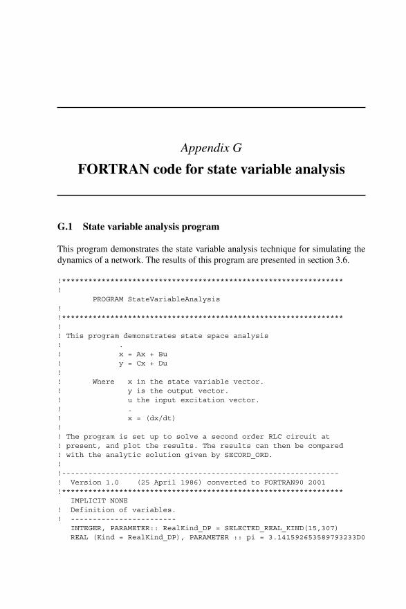
Appendix G
FORTRAN code for state variable analysis
G.1 State variable analysis program
This program demonstrates the state variable analysis technique for simulating thedynamics of a network. The results of this program are presented in section 3.6.
!****************************************************************!
PROGRAM StateVariableAnalysis!!****************************************************************!! This program demonstrates state space analysis! .! x = Ax + Bu! y = Cx + Du!! Where x in the state variable vector.! y is the output vector.! u the input excitation vector.! .! x = (dx/dt)!! The program is set up to solve a second order RLC circuit at! present, and plot the results. The results can then be compared! with the analytic solution given by SECORD_ORD.!!---------------------------------------------------------------! Version 1.0 (25 April 1986) converted to FORTRAN90 2001!****************************************************************
IMPLICIT NONE! Definition of variables.! ------------------------
INTEGER, PARAMETER:: RealKind_DP = SELECTED_REAL_KIND(15,307)REAL (Kind = RealKind_DP), PARAMETER :: pi = 3.141592653589793233D0

390 Power systems electromagnetic transients simulation
INTEGER :: Iter_Count ! Iteration CounterINTEGER :: Step_CHG_Count ! Counts the number of step changes that
! have occured in this time-stepREAL (Kind = RealKind_DP) :: Xt(2) ! State variable vector
! at Time=tREAL (Kind = RealKind_DP) :: Xth(2) ! State variable vector
! at Time=t+hREAL (Kind = RealKind_DP) :: XtDot(2) ! Derivative of state
! variables at Time=tREAL (Kind = RealKind_DP) :: XthDot(2) ! Derivative of state
! variables at Time=t+hREAL (Kind = RealKind_DP) :: XthO(2) ! Previous iterations
! estimate for state! variables at t+h
REAL (Kind = RealKind_DP) :: XthDotO(2) ! Previous iterations! estimate for derivative! of state variables at t+h
REAL (Kind = RealKind_DP) :: h ! Step lengthREAL (Kind = RealKind_DP) :: Time ! Current TimeREAL (Kind = RealKind_DP) :: Switch_Time ! Switching TimeREAL (Kind = RealKind_DP) :: Time_Left ! Time left until switchingREAL (Kind = RealKind_DP) :: Finish_Time ! Simulation Finish TimeREAL (Kind = RealKind_DP) :: StepWidth ! Step WidthREAL (Kind = RealKind_DP) :: StepWidthNom! Step WidthREAL (Kind = RealKind_DP) :: EPS ! Convergence toleranceREAL (Kind = RealKind_DP) :: R,L,C ! Circuit ParametersREAL (Kind = RealKind_DP) :: E ! Source VoltageREAL (Kind = RealKind_DP) :: f_res ! Resonant Frequency
CHARACTER*1 CHARBCHARACTER*10 CHARB2
LOGICAL :: STEP_CHG ! Step ChangeLOGICAL :: CONVG ! ConvergedLOGICAL :: Check_SVDot ! Check Derivative of State VariableLOGICAL :: OptimizeStep ! Optimize Step length
COMMON/COMPONENTS/R,L,C,E
! Initialize variables.! ---------------------
Time = 0.0Xt(1) = 0.0Xt(2) = 0.0E=0.0Switch_Time =0.1D-3 ! Seconds
Check_SVDot=.FALSE.OptimizeStep=.FALSE.
OPEN(Unit=1,STATUS=’OLD’,file=’SV_RLC.DAT’)READ(1,*) R,L,CREAD(1,*) EPS,Check_SVDot,OptimizeStep

FORTRAN code for state variable analysis 391
READ(1,*) Finish_TimeCLOSE(1)
f_res=1.0/(2.0*pi*sqrt(L*C))WRITE(6,*) R,L,C,f_res,1./f_resWRITE(6,*) ’Tolerance =’,EPSWRITE(6,*) ’Check State Variable Derivatives ’,Check_SVDotWRITE(6,*) ’Optimize step-length ’,OptimizeStepWRITE(6,*) ’Finish Time ’,Finish_Time
! Put header on file.! -------------------
OPEN(UNIT=98,status=’unknown’,file=’SVanalysis.out’)WRITE(98,9860)R,L,C,E
9860 FORMAT(1X,’%R = ’,F8.3,’ Ohms L = ’,F8.5,’ Henries C = ’,G16.5,’Farads E = ’,F8.3) WRITE(98,9870)
9870 FORMAT(1X,’% Time’,7X,’X(1)’,7X,’X(2)’,6X,’STEP W’,2X,’No. iter.’,&
& ’ XDot(1)’,’ XDot(2)’)
StepWidth = 0.05D08 WRITE(6,’(/X,A,F8.6,A)’)’Default = ’,STEPWIDTH,’ msec.’
WRITE(6,’(1X,A,$)’)’Enter Nominal stepwidth. (msec.) : ’READ(5,’(A)’)CHARB2IF(CHARB2.NE.’ ’) READ(CHARB2,’(BN,F8.4)’,ERR=8) StepWidthwrite(6,*)’StepWidth=’,StepWidth,’ msec.’pauseStepWidth = StepWidth/1000.0D0
CALL XDot (Xt,XtDot)WRITE(98,9880)TIME,Xt(1),Xt(2),H,Iter_Count,XtDot(1),XtDot(2)
DO WHILE(TIME .LE. Finish_Time)h = StepWidth
! Limit step to fall on required switching instant! ------------------------------------------------
Time_Left= Switch_Time-TimeIF(Time_Left .GT.0.0D0 .AND. Time_Left.LE.h) THEN
h = Time_LeftEND IF
XthDot(1) = XtDot(1)XthDot(2) = XtDot(2)CONVG=.FALSE.
Step_CHG_Count=0
XthO(1) = Xth(1)XthO(2) = Xth(2)XthDotO(1) = XthDot(1)XthDotO(2) = XthDot(2)
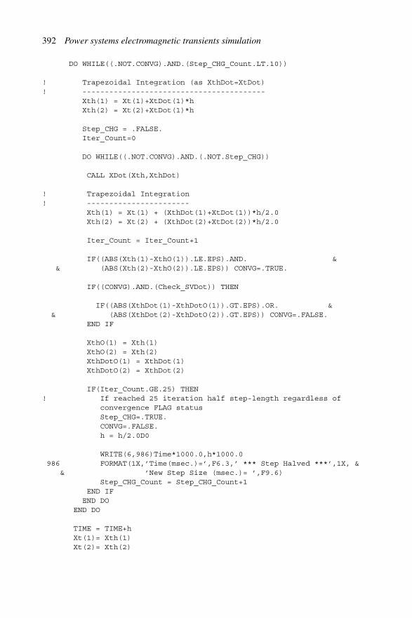
392 Power systems electromagnetic transients simulation
DO WHILE((.NOT.CONVG).AND.(Step_CHG_Count.LT.10))
! Trapezoidal Integration (as XthDot=XtDot)! -----------------------------------------
Xth(1) = Xt(1)+XtDot(1)*hXth(2) = Xt(2)+XtDot(1)*h
Step_CHG = .FALSE.Iter_Count=0
DO WHILE((.NOT.CONVG).AND.(.NOT.Step_CHG))
CALL XDot(Xth,XthDot)
! Trapezoidal Integration! -----------------------
Xth(1) = Xt(1) + (XthDot(1)+XtDot(1))*h/2.0Xth(2) = Xt(2) + (XthDot(2)+XtDot(2))*h/2.0
Iter_Count = Iter_Count+1
IF((ABS(Xth(1)-XthO(1)).LE.EPS).AND. && (ABS(Xth(2)-XthO(2)).LE.EPS)) CONVG=.TRUE.
IF((CONVG).AND.(Check_SVDot)) THEN
IF((ABS(XthDot(1)-XthDotO(1)).GT.EPS).OR. && (ABS(XthDot(2)-XthDotO(2)).GT.EPS)) CONVG=.FALSE.
END IF
XthO(1) = Xth(1)XthO(2) = Xth(2)XthDotO(1) = XthDot(1)XthDotO(2) = XthDot(2)
IF(Iter_Count.GE.25) THEN! If reached 25 iteration half step-length regardless of
convergence FLAG statusStep_CHG=.TRUE.CONVG=.FALSE.h = h/2.0D0
WRITE(6,986)Time*1000.0,h*1000.0986 FORMAT(1X,’Time(msec.)=’,F6.3,’ *** Step Halved ***’,1X, &
& ’New Step Size (msec.)= ’,F9.6)Step_CHG_Count = Step_CHG_Count+1
END IFEND DO
END DO
TIME = TIME+hXt(1)= Xth(1)Xt(2)= Xth(2)

FORTRAN code for state variable analysis 393
XtDot(1) = XthDot(1)XtDot(2) = XthDot(2)
IF(Step_CHG_Count.GE.10) THENWRITE(6,’(/X,A)’)’FAILED TO CONVERGE’WRITE(98,’(/X,A)’)’FAILED TO CONVERGE’STOP
ELSE IF(OptimizeStep) THEN! Optimize Step Length based on step length and number of! iterations.IF(Iter_Count.LE.5) THEN
StepWidth = h*1.10TYPE *,’Step-length increased by 10%’
ELSE IF(Iter_Count.GE.15) THENStepWidth = h*0.9TYPE *,’Step-length decreased by 10%’
END IFEND IFIF (Iter_Count.EQ.25) THEN
TYPE *,’How come?’TYPE *,’Time (msec.)=’,TIME*1000.0TYPE *,’CONVG=’,CONVGpause
END IF
WRITE(98,9880)TIME*1000.0,Xt(1),Xt(2),h*1000.0,Iter_Count,XtDot(1),XtDot(2)
9880 FORMAT(2X,F8.6,3X,F10.6,3X,F10.6,5X,F10.7,2X,I2,2X,F16.5,2X,F12.5)
IF(abs(Switch_Time-Time).LE.1.0E-10) THEN! State Variable can not change instantaneously hence are! the same! but dependent variables need updating. i.e. the derivative! of state variables! as well as those that are functions of state variables! or their derivative.! now two time points for the same time.E = 1.0CALL XDot(Xt,XtDot)WRITE(98,9880)TIME*1000.0,Xt(1),Xt(2),h*1000.0,Iter_Count,XtDot(1),XtDot(2)
END IFEND DOCLOSE(98)TYPE *,’ *** THE END ***’END

394 Power systems electromagnetic transients simulation
!*******************************************************SUBROUTINE XDot(SVV,DSVV)
! .! X = [A]X+[B]U!*******************************************************
! SVV = State variable vector! DSVV = Derivative of state variable vector! X(1) = Capacitor Voltage! X(2) = Inductor Current
IMPLICIT NONE
INTEGER, PARAMETER:: RealKind_DP = SELECTED_REAL_KIND(15,307)
REAL (Kind = RealKind_DP) :: SVV(2),DSVV(2)REAL (Kind = RealKind_DP) :: R,L,C,ECOMMON/COMPONENTS/R,L,C,E
DSVV(1) = SVV(2)/CDSVV(2) =-SVV(1)/L-SVV(2)*R/L+E/L
RETURNEND
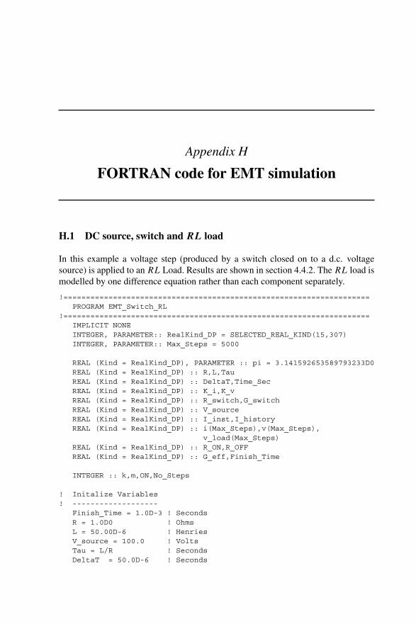
Appendix H
FORTRAN code for EMT simulation
H.1 DC source, switch and RL load
In this example a voltage step (produced by a switch closed on to a d.c. voltagesource) is applied to an RL Load. Results are shown in section 4.4.2. The RL load ismodelled by one difference equation rather than each component separately.
!====================================================================PROGRAM EMT_Switch_RL
!====================================================================IMPLICIT NONEINTEGER, PARAMETER:: RealKind_DP = SELECTED_REAL_KIND(15,307)INTEGER, PARAMETER:: Max_Steps = 5000
REAL (Kind = RealKind_DP), PARAMETER :: pi = 3.141592653589793233D0REAL (Kind = RealKind_DP) :: R,L,TauREAL (Kind = RealKind_DP) :: DeltaT,Time_SecREAL (Kind = RealKind_DP) :: K_i,K_vREAL (Kind = RealKind_DP) :: R_switch,G_switchREAL (Kind = RealKind_DP) :: V_sourceREAL (Kind = RealKind_DP) :: I_inst,I_historyREAL (Kind = RealKind_DP) :: i(Max_Steps),v(Max_Steps),
v_load(Max_Steps)REAL (Kind = RealKind_DP) :: R_ON,R_OFFREAL (Kind = RealKind_DP) :: G_eff,Finish_Time
INTEGER :: k,m,ON,No_Steps
! Initalize Variables! -------------------
Finish_Time = 1.0D-3 ! SecondsR = 1.0D0 ! OhmsL = 50.00D-6 ! HenriesV_source = 100.0 ! VoltsTau = L/R ! SecondsDeltaT = 50.0D-6 ! Seconds

396 Power systems electromagnetic transients simulation
R_ON = 1.0D-10 ! OhmsR_OFF = 1.0D10 ! OhmsR_Switch = R_OFF ! OhmsON = 0 ! Initially switch is open
m = 1i(m) = 0.0Time_Sec = 0.0v(m) =100.0v_load(m) = 0.0
K_i = (1-DeltaT*R/(2*L))/(1+DeltaT*R/(2*L))K_v = (DeltaT/(2*L))/(1+DeltaT*R/(2*L))G_eff = K_vG_switch = 1.0/R_switch
OPEN (unit=10,status=’unknown’,file=’SwitchRL1.out’)
No_Steps= Finish_Time/DeltaTIF(Max_Steps<No_Steps) THEN
STOP ’*** Too Many Steps ***’END IFMainLoop: DO k=1,No_Steps,1
m=m+1Time_Sec = k*DeltaT
! Check Switch position! ---------------------
IF(k==3) THENON = 1R_switch = R_ONG_switch = 1.0/R_switch
END IF
! Update History term! -------------------
I_history = k_i*i(m-1) + k_v*v_load(m-1)
! Update Voltage Sources! ----------------------
v(m) = V_source
! Solve for V and I! -----------------
v_load(m) = (-I_history + v(m)* G_switch)/(G_eff+G_Switch)I_inst = v_load(m)*G_effi(m) = I_inst + I_historywrite(10,*) Time_Sec,v_load(m),i(m)
END DO MainLoopCLOSE(10)PRINT *,’ Execution Finished’
END PROGRAM EMT_Switch_RL

FORTRAN code for EMT simulation 397
H.2 General EMT program for d.c. source, switch and RL load
The same case as in section H.1 is modelled here, however, the program is nowstructured in a general manner, where each component is subjected to numericalintegrator substitution (NIS) and the conductance matrix is built up. Moreover, ratherthan modelling the switch as a variable resistor, matrix partitioning is applied (seesection 4.4.1), which enables the use of ideal switches.
!===============================!
PROGRAM EMT_Switch_RL!! Checked and correct 4 May 2001!===============================
IMPLICIT NONE! INTEGER SELECT_REAL_KIND!INTEGER ,PARAMETER:: Real_18_4931 =SELECT_REAL_KIND(P=18,R=4931)
REAL*8 :: R,L,TcREAL*8 :: DeltaTREAL*8 :: i_L,i_R,i_Source,i_Source2REAL*8 :: R_switch,G_switchREAL*8 :: G(3,3),v(3),I_Vector(2)REAL*8 :: G_L,G_RREAL*8 :: V_sourceREAL*8 :: I_L_historyREAL*8 :: MultiplierREAL*8 :: R_ON,R_OFF
INTEGER k,n,NoTimeStepsINTEGER NoColumns
open(unit=11,status=’unknown’,file=’vi.out’)
NoTimeSteps = 6NoColumns = 3R_ON = 1.0D-10 ! OhmsR_OFF = 1.0D+10 ! Ohms
DeltaT = 50.0D-6 ! Seconds
R = 1.0D0 ! OhmsL = 50.00D-6 ! HenriesV_source=100 ! VoltsTc = L/RPRINT *,’Time Constant=’,TcR_switch = R_OFFG_switch = 1/R_switchG_R = 1/RG_L = DeltaT/(2*L) ! G_L_eff

398 Power systems electromagnetic transients simulation
! Initialize Variables! --------------------
I_Vector(1) =0.0D0I_Vector(2) =0.0D0i_L =0.0D0DO k=1,3
v(k) = 0.000D0END DO
! Form System Conductance Matrix! ------------------------------
CALL Form_G(G_R,G_L,G_switch,G)
! Forward Reduction! -----------------
CALL Forward_Reduction_G(NoColumns,G,Multiplier)
! Enter Main Time-stepping loop! -----------------------------
DO n=1,NoTimeSteps
IF(n==1)THENwrite(10, *) ’ Switch Turned ON’R_switch = R_ONG_switch = 1/R_switch
CALL Form_G(G_R,G_L,G_switch,G)CALL Forward_Reduction_G(NoColumns,G,Multiplier)
END IF
! Calculate Past History Terms! ----------------------------
I_L_history =i_L + v(3)*G_LI_Vector(1) = 0.0I_Vector(2) = -I_L_history
! Update Source Values! --------------------
V_source = 100.0V(1) = V_source
! Forward Reduction of Current Vector! -----------------------------------
I_Vector(2) = I_Vector(2) - Multiplier*I_Vector(1)
! Move Known Voltage to RHS (I_current Vector)! --------------------------------------------
I_Vector(1) = I_Vector(1)- G(1,3) * V(1)I_Vector(2) = I_Vector(2)- G(2,3) * V(1)
! Back-substitution! -----------------
v(3) = I_Vector(2)/G(2,2)v(2) = (I_Vector(1)-G(1,2)*v(3))/G(1,1)

FORTRAN code for EMT simulation 399
! Calculate Branch Current! ------------------------
i_R = (v(2) - v(3))/Ri_L = v(3)*G_L + I_L_historyi_Source2 = (v(1)-v(2))*G_switchi_Source = G(3,1)*v(2) + G(3,2)*v(3) + G(3,3)*v(1)
WRITE(11,1160) n*DeltaT,v(1),v(2),v(3),i_Source,i_R,i_L
END DOclose(11)
1160 FORMAT(1X,F8.6,1X,6(G16.10,1X))STOPEND
!====================================================SUBROUTINE Form_G(G_R,G_L,G_switch,G)
!====================================================IMPLICIT NONEREAL*8 :: G(3,3)REAL*8 :: G_L,G_R,G_switch
G(1,1) = G_switch + G_RG(2,1) = - G_RG(1,2) = - G_R
G(2,2) = G_L + G_RG(1,3) = -G_switchG(2,3) = 0.0D0
G(3,1) = -G_switchG(3,2) = 0.0D0G(3,3) = G_switch
CALL Show_G(G)RETURNEND
!====================================================SUBROUTINE Forward_Reduction_G(NoColumns,G,Multiplier)
!====================================================IMPLICIT NONEREAL*8 :: G(3,3)REAL*8 :: MultiplierINTEGER :: k,NoColumns
Multiplier = G(2,1)/G(1,1)PRINT *,’ Multiplier= ’,Multiplier
DO k=1,NoColumnsG(2,k) = G(2,k) - Multiplier*G(1,k)
END DO
RETURNEND
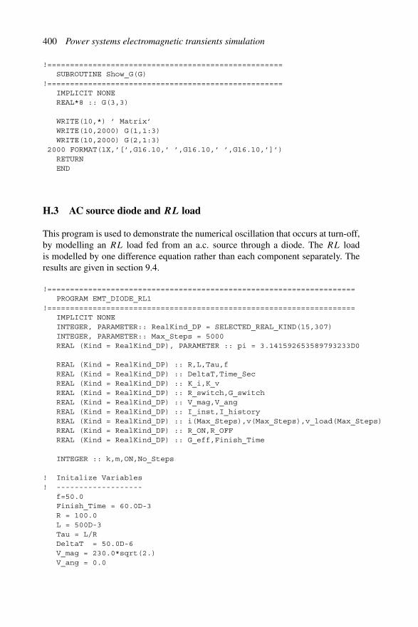
400 Power systems electromagnetic transients simulation
!====================================================SUBROUTINE Show_G(G)
!====================================================IMPLICIT NONEREAL*8 :: G(3,3)
WRITE(10,*) ’ Matrix’WRITE(10,2000) G(1,1:3)WRITE(10,2000) G(2,1:3)
2000 FORMAT(1X,’[’,G16.10,’ ’,G16.10,’ ’,G16.10,’]’)RETURNEND
H.3 AC source diode and RL load
This program is used to demonstrate the numerical oscillation that occurs at turn-off,by modelling an RL load fed from an a.c. source through a diode. The RL loadis modelled by one difference equation rather than each component separately. Theresults are given in section 9.4.
!====================================================================PROGRAM EMT_DIODE_RL1
!====================================================================IMPLICIT NONEINTEGER, PARAMETER:: RealKind_DP = SELECTED_REAL_KIND(15,307)INTEGER, PARAMETER:: Max_Steps = 5000REAL (Kind = RealKind_DP), PARAMETER :: pi = 3.141592653589793233D0
REAL (Kind = RealKind_DP) :: R,L,Tau,fREAL (Kind = RealKind_DP) :: DeltaT,Time_SecREAL (Kind = RealKind_DP) :: K_i,K_vREAL (Kind = RealKind_DP) :: R_switch,G_switchREAL (Kind = RealKind_DP) :: V_mag,V_angREAL (Kind = RealKind_DP) :: I_inst,I_historyREAL (Kind = RealKind_DP) :: i(Max_Steps),v(Max_Steps),v_load(Max_Steps)REAL (Kind = RealKind_DP) :: R_ON,R_OFFREAL (Kind = RealKind_DP) :: G_eff,Finish_Time
INTEGER :: k,m,ON,No_Steps
! Initalize Variables! -------------------
f=50.0Finish_Time = 60.0D-3R = 100.0L = 500D-3Tau = L/RDeltaT = 50.0D-6V_mag = 230.0*sqrt(2.)V_ang = 0.0

FORTRAN code for EMT simulation 401
R_ON = 1.0D-10R_OFF = 1.0D10R_Switch = R_ON
m=1i(m) = 0.0Time_Sec = 0.0v(m) = V_mag*sin(V_ang*pi/180)v_load(m)=v(m)ON=1K_i = (1-DeltaT*R/(2*L))/(1+DeltaT*R/(2*L))K_v = (DeltaT/(2*L))/(1+DeltaT*R/(2*L))G_eff = K_vG_switch = 1.0/R_switch
OPEN (unit=10,status=’unknown’,file=’DiodeRL1.out’)
No_Steps= Finish_Time/DeltaTIF(Max_Steps<No_Steps) THEN
STOP ’*** Too Many Steps ***’END IF
MainLoop: DO k=1,No_Steps,1m=m+1Time_Sec = k*DeltaT
! Check Switch position! ---------------------
IF (i(m-1)<= 0.0 .and. ON==1 .and. k >5*DeltaT) THENON = 0R_switch = R_OFFG_switch = 1.0/R_switchi(m-1) = 0.0
END IFIF (v(m-1)-v_load(m-1) > 1.0 .and. ON==0) THEN
ON = 1R_switch = R_ONG_switch = 1.0/R_switch
END IF
! Update History term! -------------------
I_history = k_i*i(m-1) + k_v*v_load(m-1)
! Update Voltage Sources! ----------------------
v(m) = V_mag*sin(2*pi*f*Time_Sec + V_ang*pi/180)
! Solve for V and I! -----------------
v_load(m) = (-I_history + v(m)* G_switch)/(G_eff+G_Switch)I_inst = v_load(m)*G_eff

402 Power systems electromagnetic transients simulation
i(m) = I_inst + I_historywrite(10,*) Time_Sec,v_load(m),i(m)
END DO MainLoopCLOSE(10)
PRINT *,’ Execution Finished’
END PROGRAM EMT_DIODE_RL1
H.4 Simple lossless transmission line
This program evaluates the step response of a simple lossless transmission line, asshown in section 6.6.
!==========================================================PROGRAM Lossless_TL
!! A simple lossless travelling wave transmission line!==========================================================
IMPLICIT NONEINTEGER, PARAMETER:: RealKind_DP = SELECTED_REAL_KIND(15,307)INTEGER, PARAMETER:: TL_BufferSize = 100
! Transmission Line Buffer! ------------------------
REAL (Kind=RealKind_DP) :: Vsend(TL_BufferSize)REAL (Kind=RealKind_DP) :: Vrecv(TL_BufferSize)REAL (Kind=RealKind_DP) :: Isend_Hist(TL_BufferSize)REAL (Kind=RealKind_DP) :: Irecv_Hist(TL_BufferSize)
REAL (Kind=RealKind_DP) :: L_dash,C_dash,LengthREAL (Kind=RealKind_DP) :: DeltaTREAL (Kind=RealKind_DP) :: TimeREAL (Kind=RealKind_DP) :: R_Source,R_LoadREAL (Kind=RealKind_DP) :: V_Source,I_SourceREAL (Kind=RealKind_DP) :: Gsend,Grecv,Rsend,RrecvREAL (Kind=RealKind_DP) :: Zc, GammaREAL (Kind=RealKind_DP) :: Finish_Time,Step_TimeREAL (Kind=RealKind_DP) :: i_send ! Sending to Receiving end currentREAL (Kind=RealKind_DP) :: i_recv ! Receiving to Sending end current
INTEGER PositionINTEGER PreviousHistoryPSNINTEGER k,NumberSteps,Step_NoINTEGER No_Steps_Delay
OPEN(UNIT=10,file=’TL.out’,status="UNKNOWN")
! Default Line Parameters! -----------------------
L_dash = 400D-9
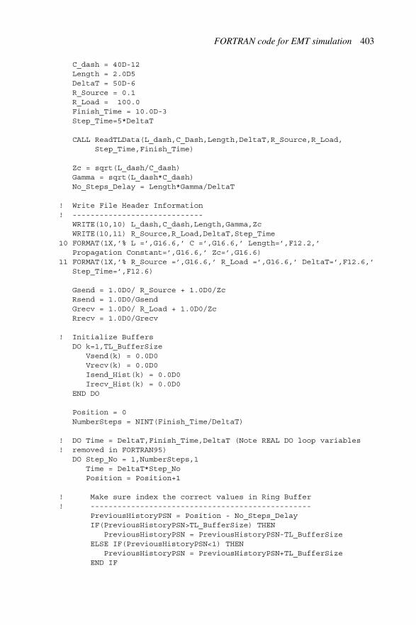
FORTRAN code for EMT simulation 403
C_dash = 40D-12Length = 2.0D5DeltaT = 50D-6R_Source = 0.1R_Load = 100.0Finish_Time = 10.0D-3Step_Time=5*DeltaT
CALL ReadTLData(L_dash,C_Dash,Length,DeltaT,R_Source,R_Load,Step_Time,Finish_Time)
Zc = sqrt(L_dash/C_dash)Gamma = sqrt(L_dash*C_dash)No_Steps_Delay = Length*Gamma/DeltaT
! Write File Header Information! -----------------------------
WRITE(10,10) L_dash,C_dash,Length,Gamma,ZcWRITE(10,11) R_Source,R_Load,DeltaT,Step_Time
10 FORMAT(1X,’% L =’,G16.6,’ C =’,G16.6,’ Length=’,F12.2,’Propagation Constant=’,G16.6,’ Zc=’,G16.6)
11 FORMAT(1X,’% R_Source =’,G16.6,’ R_Load =’,G16.6,’ DeltaT=’,F12.6,’Step_Time=’,F12.6)
Gsend = 1.0D0/ R_Source + 1.0D0/ZcRsend = 1.0D0/GsendGrecv = 1.0D0/ R_Load + 1.0D0/ZcRrecv = 1.0D0/Grecv
! Initialize BuffersDO k=1,TL_BufferSize
Vsend(k) = 0.0D0Vrecv(k) = 0.0D0Isend_Hist(k) = 0.0D0Irecv_Hist(k) = 0.0D0
END DO
Position = 0NumberSteps = NINT(Finish_Time/DeltaT)
! DO Time = DeltaT,Finish_Time,DeltaT (Note REAL DO loop variables! removed in FORTRAN95)
DO Step_No = 1,NumberSteps,1Time = DeltaT*Step_NoPosition = Position+1
! Make sure index the correct values in Ring Buffer! -------------------------------------------------
PreviousHistoryPSN = Position - No_Steps_DelayIF(PreviousHistoryPSN>TL_BufferSize) THEN
PreviousHistoryPSN = PreviousHistoryPSN-TL_BufferSizeELSE IF(PreviousHistoryPSN<1) THEN
PreviousHistoryPSN = PreviousHistoryPSN+TL_BufferSizeEND IF

404 Power systems electromagnetic transients simulation
IF(Position>TL_BufferSize) THENPosition = Position-TL_BufferSize
END IF
! Update Sources! --------------
IF(Time< 5*DeltaT) THENV_Source = 0.0
ELSEV_Source = 100.0
END IFI_Source = V_Source/R_Source
! Solve for Nodal Voltages! ------------------------
Vsend(Position) = (I_Source-Isend_Hist(PreviousHistoryPSN))*RsendVrecv(Position) = ( -Irecv_Hist(PreviousHistoryPSN))*Rrecv
! Solve for Terminal Current! --------------------------
i_send = Vsend(Position)/Zc + Isend_Hist(PreviousHistoryPSN)i_recv = Vrecv(Position)/Zc + Irecv_Hist(PreviousHistoryPSN)
! Calculate History Term (Current Source at tau later).! -----------------------------------------------------
Irecv_Hist(Position) = (-1.0/Zc)*Vsend(Position) - i_sendIsend_Hist(Position) = (-1.0/Zc)*Vrecv(Position) - i_recv
WRITE(10,1000) Time,Vsend(Position),Vrecv(Position),i_send,i_recv,Isend_Hist(Position),Irecv_Hist(Position)
END DO1000 FORMAT(1X,7(G16.6,1X))
CLOSE(10)
PRINT *,’ Successful Completion’END
H.5 Bergeron transmission line
In this example the step response of a simple transmission line with lumped losses(Bergeron model) is evaluated (see section 6.6).
!==========================================================PROGRAM TL_Bergeron
! Bergeron Line Model (Lumped representation of Losses)!==========================================================
IMPLICIT NONEINTEGER, PARAMETER:: RealKind_DP = SELECTED_REAL_KIND(15,307)INTEGER, PARAMETER:: TL_BufferSize = 100

FORTRAN code for EMT simulation 405
! Transmission Line Buffer! ------------------------
REAL (Kind=RealKind_DP) :: Vsend(TL_BufferSize)REAL (Kind=RealKind_DP) :: Vrecv(TL_BufferSize)REAL (Kind=RealKind_DP) :: Isend_Hist(TL_BufferSize)REAL (Kind=RealKind_DP) :: Irecv_Hist(TL_BufferSize)
REAL (Kind=RealKind_DP) :: R_dash,L_dash,C_dash,LengthREAL (Kind=RealKind_DP) :: DeltaT,TimeREAL (Kind=RealKind_DP) :: R,R_Source,R_LoadREAL (Kind=RealKind_DP) :: V_Source,I_SourceREAL (Kind=RealKind_DP) :: Gsend,Grecv,Rsend,RrecvREAL (Kind=RealKind_DP) :: Zc, Zc_Plus_R4,GammaREAL (Kind=RealKind_DP) :: Finish_Time,Step_TimeREAL (Kind=RealKind_DP) :: i_send ! Sending to Receiving end currentREAL (Kind=RealKind_DP) :: i_recv ! Receiving to Sending end current
INTEGER PositionINTEGER PreviousHistoryPSNINTEGER k,NumberSteps,Step_NoINTEGER No_Steps_Delay
OPEN(UNIT=10,file=’TL.out’,status="UNKNOWN")
R_dash = 100D-6L_dash = 400D-9C_dash = 40D-12Length = 2.0D5DeltaT = 50D-6R_Source = 0.1R_Load = 100.0Finish_Time = 1.0D-4Step_Time=5*DeltaT
CALL ReadTLData(R_dash,L_dash,C_Dash,Length,DeltaT,R_Source,R_Load,Step_Time,Finish_Time)
R=R_Dash*Length
Zc = sqrt(L_dash/C_dash)Gamma = sqrt(L_dash*C_dash)No_Steps_Delay = Length*Gamma/DeltaTZc_Plus_R4 = Zc+R/4.0
! Write File Header Information! -----------------------------
WRITE(10,10) R_dash,L_dash,C_dash,Length,Gamma,ZcWRITE(10,11) R_Source,R_Load,DeltaT,Step_Time
10 FORMAT(1X,’% R =’,G16.6,’ L =’,G16.6,’ C =’,G16.6,’ Length=’,F12.2,’Propagation Constant=’,G16.6,’ Zc=’,G16.6)
11 FORMAT(1X,’% R_Source =’,G16.6,’ R_Load =’,G16.6,’ DeltaT=’,F12.6,’Step_Time=’,F12.6)
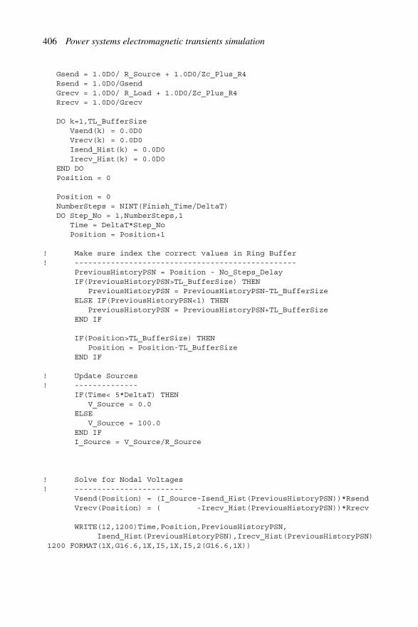
406 Power systems electromagnetic transients simulation
Gsend = 1.0D0/ R_Source + 1.0D0/Zc_Plus_R4Rsend = 1.0D0/GsendGrecv = 1.0D0/ R_Load + 1.0D0/Zc_Plus_R4Rrecv = 1.0D0/Grecv
DO k=1,TL_BufferSizeVsend(k) = 0.0D0Vrecv(k) = 0.0D0Isend_Hist(k) = 0.0D0Irecv_Hist(k) = 0.0D0
END DOPosition = 0
Position = 0NumberSteps = NINT(Finish_Time/DeltaT)DO Step_No = 1,NumberSteps,1
Time = DeltaT*Step_NoPosition = Position+1
! Make sure index the correct values in Ring Buffer! -------------------------------------------------
PreviousHistoryPSN = Position - No_Steps_DelayIF(PreviousHistoryPSN>TL_BufferSize) THEN
PreviousHistoryPSN = PreviousHistoryPSN-TL_BufferSizeELSE IF(PreviousHistoryPSN<1) THEN
PreviousHistoryPSN = PreviousHistoryPSN+TL_BufferSizeEND IF
IF(Position>TL_BufferSize) THENPosition = Position-TL_BufferSize
END IF
! Update Sources! --------------
IF(Time< 5*DeltaT) THENV_Source = 0.0
ELSEV_Source = 100.0
END IFI_Source = V_Source/R_Source
! Solve for Nodal Voltages! ------------------------
Vsend(Position) = (I_Source-Isend_Hist(PreviousHistoryPSN))*RsendVrecv(Position) = ( -Irecv_Hist(PreviousHistoryPSN))*Rrecv
WRITE(12,1200)Time,Position,PreviousHistoryPSN,Isend_Hist(PreviousHistoryPSN),Irecv_Hist(PreviousHistoryPSN)
1200 FORMAT(1X,G16.6,1X,I5,1X,I5,2(G16.6,1X))

FORTRAN code for EMT simulation 407
! Solve for Terminal Current! --------------------------
i_send = Vsend(Position)/Zc_Plus_R4 + Isend_Hist(PreviousHistoryPSN)i_recv = Vrecv(Position)/Zc_Plus_R4 + Irecv_Hist(PreviousHistoryPSN)
! Calculate History Term (Current Source at tau later).! -----------------------------------------------------
Irecv_Hist(Position) = (-Zc/(Zc_Plus_R4**2))*(Vsend(Position)+(Zc-R/4.0)*i_send) &+((-R/4.0)/(Zc_Plus_R4**2))*(Vrecv(Position)+(Zc-R/4.0)*i_recv)
Isend_Hist(Position) = (-Zc/(Zc_Plus_R4**2))*(Vrecv(Position)+(Zc-R/4.0)*i_recv) &+((-R/4.0)/(Zc_Plus_R4**2))*(Vsend(Position)+(Zc-R/4.0)*i_send)
WRITE(10,1000) Time,Vsend(Position),Vrecv(Position),i_send,i_recv,Isend_Hist(Position),Irecv_Hist(Position)
END DO1000 FORMAT(1X,7(G16.6,1X))
CLOSE(10)PRINT *,’ Successful Completion’END
H.6 Frequency-dependent transmission line
This program demonstrates the implementation of a full frequency-dependent trans-mission line and allows the step response to be determined. This is an s-domainimplementation using recursive convolution. For simplicity interpolation of buffervalues is not included. Results are illustrated in section 6.6.
!==========================================================PROGRAM TL_FDP_s
!! Simple Program to demonstrate the implementation of a! Frequency-Dependent Transmission Line using s-domain representation.!! Isend(w) Irecv(w)! ------>---- ------<-----! | |! -------- --------! | | | |! _|__ / / _|__! | | / ˆ / ˆ | |! Vs(w) |Yc| | / | / |Yc| Vr(w)! |__| / / |__|! | | Ih_s | Ih_r |! -------- --------! | |! ----------- ------------!!==========================================================
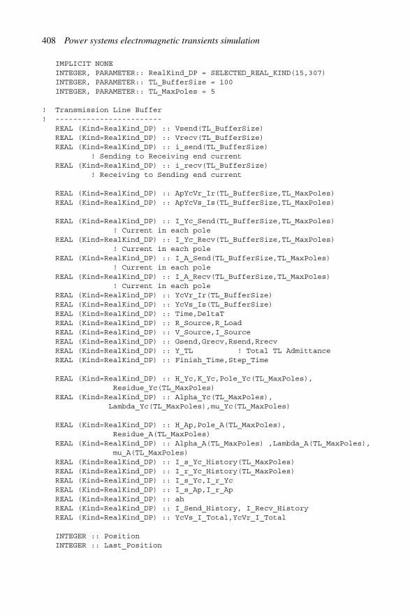
408 Power systems electromagnetic transients simulation
IMPLICIT NONEINTEGER, PARAMETER:: RealKind_DP = SELECTED_REAL_KIND(15,307)INTEGER, PARAMETER:: TL_BufferSize = 100INTEGER, PARAMETER:: TL_MaxPoles = 5
! Transmission Line Buffer! ------------------------
REAL (Kind=RealKind_DP) :: Vsend(TL_BufferSize)REAL (Kind=RealKind_DP) :: Vrecv(TL_BufferSize)REAL (Kind=RealKind_DP) :: i_send(TL_BufferSize)
! Sending to Receiving end currentREAL (Kind=RealKind_DP) :: i_recv(TL_BufferSize)
! Receiving to Sending end current
REAL (Kind=RealKind_DP) :: ApYcVr_Ir(TL_BufferSize,TL_MaxPoles)REAL (Kind=RealKind_DP) :: ApYcVs_Is(TL_BufferSize,TL_MaxPoles)
REAL (Kind=RealKind_DP) :: I_Yc_Send(TL_BufferSize,TL_MaxPoles)! Current in each pole
REAL (Kind=RealKind_DP) :: I_Yc_Recv(TL_BufferSize,TL_MaxPoles)! Current in each pole
REAL (Kind=RealKind_DP) :: I_A_Send(TL_BufferSize,TL_MaxPoles)! Current in each pole
REAL (Kind=RealKind_DP) :: I_A_Recv(TL_BufferSize,TL_MaxPoles)! Current in each pole
REAL (Kind=RealKind_DP) :: YcVr_Ir(TL_BufferSize)REAL (Kind=RealKind_DP) :: YcVs_Is(TL_BufferSize)REAL (Kind=RealKind_DP) :: Time,DeltaTREAL (Kind=RealKind_DP) :: R_Source,R_LoadREAL (Kind=RealKind_DP) :: V_Source,I_SourceREAL (Kind=RealKind_DP) :: Gsend,Grecv,Rsend,RrecvREAL (Kind=RealKind_DP) :: Y_TL ! Total TL AdmittanceREAL (Kind=RealKind_DP) :: Finish_Time,Step_Time
REAL (Kind=RealKind_DP) :: H_Yc,K_Yc,Pole_Yc(TL_MaxPoles),Residue_Yc(TL_MaxPoles)
REAL (Kind=RealKind_DP) :: Alpha_Yc(TL_MaxPoles),Lambda_Yc(TL_MaxPoles),mu_Yc(TL_MaxPoles)
REAL (Kind=RealKind_DP) :: H_Ap,Pole_A(TL_MaxPoles),Residue_A(TL_MaxPoles)
REAL (Kind=RealKind_DP) :: Alpha_A(TL_MaxPoles) ,Lambda_A(TL_MaxPoles),mu_A(TL_MaxPoles)
REAL (Kind=RealKind_DP) :: I_s_Yc_History(TL_MaxPoles)REAL (Kind=RealKind_DP) :: I_r_Yc_History(TL_MaxPoles)REAL (Kind=RealKind_DP) :: I_s_Yc,I_r_YcREAL (Kind=RealKind_DP) :: I_s_Ap,I_r_ApREAL (Kind=RealKind_DP) :: ahREAL (Kind=RealKind_DP) :: I_Send_History, I_Recv_HistoryREAL (Kind=RealKind_DP) :: YcVs_I_Total,YcVr_I_Total
INTEGER :: PositionINTEGER :: Last_Position

FORTRAN code for EMT simulation 409
INTEGER :: t_tau,t_Tau_1,t_Tau_2INTEGER :: k,mINTEGER :: No_Steps_DelayINTEGER :: RecursiveConvTypeINTEGER :: No_Poles_Yc, No_Poles_A
OPEN(UNIT=10,file=’TL.out’,status="UNKNOWN")
DeltaT = 50D-6 ! Time-stepR_Source = 0.1D0 ! Source resistanceR_Load = 100.0D0Finish_Time = 1.0D-2Step_Time = 5*DeltaTRecursiveConvType = 1No_Steps_Delay = 7
! Partial Fraction Expansion of Yc and Ap! ---------------------------------------
H_Yc =0.00214018572698*0.91690065830247No_Poles_Yc = 3K_Yc = 1.0Pole_Yc(1) = -1.00514000000000D5Pole_Yc(2) = -0.00625032000000D5Pole_Yc(3) = -0.00028960740000D5
Residue_Yc(1) = -19.72605872772154D0Residue_Yc(2) = -0.14043511946635D0Residue_Yc(3) = -0.00657234249032D0
Y_TL = H_Yc*K_YcDO k=1,No_Poles_Yc
Residue_Yc(k) = H_Yc * Residue_Yc(k)END DO
! --------------- Ap -----------------------No_Poles_A=4H_Ap = 0.995Residue_A(1) = 2.13779561263148D6Residue_A(2) = -2.18582740962054D6Residue_A(3) = 0.04688271799632D6Residue_A(4) = 0.00114907899276D6
Pole_A(1) = -5.58224599999997D5Pole_A(2) = -5.46982800000003D5Pole_A(3) = -0.47617630000000D5Pole_A(4) = -0.06485341000000D5
DO k=1,No_Poles_AResidue_A(k) = H_Ap * Residue_A(k)
END DO
! Initialize variables to zero! ----------------------------
Time = 0.0D0
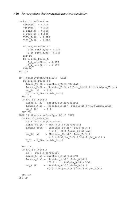
410 Power systems electromagnetic transients simulation
DO k=1,TL_BufferSizeVsend(k) = 0.0D0Vrecv(k) = 0.0D0i_send(k) = 0.0D0i_recv(k) = 0.0D0YcVs_Is(k) = 0.0D0YcVr_Ir(k) = 0.0D0
DO m=1,No_Poles_YcI_Yc_send(k,m) = 0.0D0I_Yc_recv(k,m) = 0.0D0
END DODO m=1,No_Poles_A
I_A_send(k,m) = 0.0D0I_A_recv(k,m) = 0.0D0
END DOEND DO
IF (RecursiveConvType.EQ.0) THENDO k=1,No_Poles_Yc
Alpha_Yc (k)= exp(Pole_Yc(k)*DeltaT)Lambda_Yc(k)= (Residue_Yc(k)/(-Pole_Yc(k)))*(1.0-Alpha_Yc(k))mu_Yc (k) = 0.0Y_TL = Y_TL+ Lambda_Yc(k)
END DODO k=1,No_Poles_A
Alpha_A (k) = exp(Pole_A(k)*DeltaT)Lambda_A(k) = (Residue_A(k)/(-Pole_A(k)))*(1.0-Alpha_A(k))mu_A (k) = 0.0
END DOELSE IF (RecursiveConvType.EQ.1) THEN
DO k=1,No_Poles_Ycah = -Pole_Yc(k)*DeltaTAlpha_Yc (k) = exp(Pole_Yc(k)*DeltaT)Lambda_Yc(k) = (Residue_Yc(k)/(-Pole_Yc(k)))
*(1.0 - (1.0-Alpha_Yc(k))/ah)mu_Yc (k) = (Residue_Yc(k)/(-Pole_Yc(k)))
*(((1.0-Alpha_Yc(k))/ah)-Alpha_Yc(k) )Y_TL = Y_TL+ Lambda_Yc(k)
END DODO k=1,No_Poles_A
ah = -Pole_A(k)*DeltaTAlpha_A (k) = exp(Pole_A(k)*DeltaT)Lambda_A(k) = (Residue_A(k)/(-Pole_A(k)))
*(1.0 - (1.0-Alpha_A(k))/(ah))mu_A (k) = (Residue_A(k)/(-Pole_A(k)))
*(((1.0-Alpha_A(k))/(ah))-Alpha_A(k))
END DOEND IF
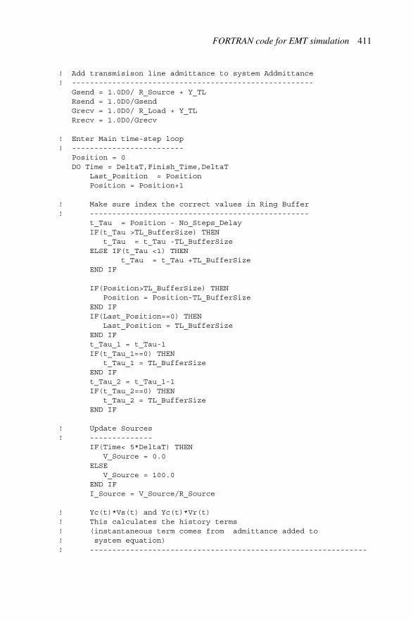
FORTRAN code for EMT simulation 411
! Add transmisison line admittance to system Addmittance! ------------------------------------------------------
Gsend = 1.0D0/ R_Source + Y_TLRsend = 1.0D0/GsendGrecv = 1.0D0/ R_Load + Y_TLRrecv = 1.0D0/Grecv
! Enter Main time-step loop! -------------------------
Position = 0DO Time = DeltaT,Finish_Time,DeltaT
Last_Position = PositionPosition = Position+1
! Make sure index the correct values in Ring Buffer! -------------------------------------------------
t_Tau = Position - No_Steps_DelayIF(t_Tau >TL_BufferSize) THEN
t_Tau = t_Tau -TL_BufferSizeELSE IF(t_Tau <1) THEN
t_Tau = t_Tau +TL_BufferSizeEND IF
IF(Position>TL_BufferSize) THENPosition = Position-TL_BufferSize
END IFIF(Last_Position==0) THEN
Last_Position = TL_BufferSizeEND IFt_Tau_1 = t_Tau-1IF(t_Tau_1==0) THEN
t_Tau_1 = TL_BufferSizeEND IFt_Tau_2 = t_Tau_1-1IF(t_Tau_2==0) THEN
t_Tau_2 = TL_BufferSizeEND IF
! Update Sources! --------------
IF(Time< 5*DeltaT) THENV_Source = 0.0
ELSEV_Source = 100.0
END IFI_Source = V_Source/R_Source
! Yc(t)*Vs(t) and Yc(t)*Vr(t)! This calculates the history terms! (instantaneous term comes from admittance added to! system equation)! --------------------------------------------------------------
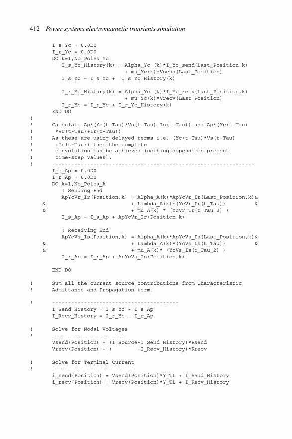
412 Power systems electromagnetic transients simulation
I_s_Yc = 0.0D0I_r_Yc = 0.0D0DO k=1,No_Poles_Yc
I_s_Yc_History(k) = Alpha_Yc (k)*I_Yc_send(Last_Position,k)+ mu_Yc(k)*Vsend(Last_Position)
I_s_Yc = I_s_Yc + I_s_Yc_History(k)
I_r_Yc_History(k) = Alpha_Yc (k)*I_Yc_recv(Last_Position,k)+ mu_Yc(k)*Vrecv(Last_Position)
I_r_Yc = I_r_Yc + I_r_Yc_History(k)END DO
!! Calculate Ap*(Yc(t-Tau)*Vs(t-Tau)+Is(t-Tau)) and Ap*(Yc(t-Tau)! *Vr(t-Tau)+Ir(t-Tau))! As these are using delayed terms i.e. (Yc(t-Tau)*Vs(t-Tau)! +Is(t-Tau)) then the complete! convolution can be achieved (nothing depends on present! time-step values).! ----------------------------------------------------------------
I_s_Ap = 0.0D0I_r_Ap = 0.0D0DO k=1,No_Poles_A
! Sending EndApYcVr_Ir(Position,k) = Alpha_A(k)*ApYcVr_Ir(Last_Position,k)&
& + Lambda_A(k)*(YcVr_Ir(t_Tau)) && + mu_A(k) * (YcVr_Ir(t_Tau_2) )
I_s_Ap = I_s_Ap + ApYcVr_Ir(Position,k)
! Receiving EndApYcVs_Is(Position,k) = Alpha_A(k)*ApYcVs_Is(Last_Position,k)&
& + Lambda_A(k)*(YcVs_Is(t_Tau)) && + mu_A(k)* (YcVs_Is(t_Tau_2) )
I_r_Ap = I_r_Ap + ApYcVs_Is(Position,k)
END DO
! Sum all the current source contributions from Characteristic! Admittance and Propagation term.
! ----------------------------------------I_Send_History = I_s_Yc - I_s_ApI_Recv_History = I_r_Yc - I_r_Ap
! Solve for Nodal Voltages! ------------------------
Vsend(Position) = (I_Source-I_Send_History)*RsendVrecv(Position) = ( -I_Recv_History)*Rrecv
! Solve for Terminal Current! --------------------------
i_send(Position) = Vsend(Position)*Y_TL + I_Send_Historyi_recv(Position) = Vrecv(Position)*Y_TL + I_Recv_History
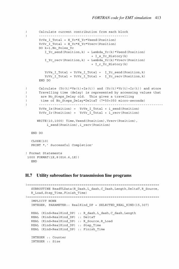
FORTRAN code for EMT simulation 413
! Calculate current contribution from each block! ----------------------------------------------
YcVs_I_Total = H_Yc*K_Yc*Vsend(Position)YcVr_I_Total = H_Yc*K_Yc*Vrecv(Position)DO k=1,No_Poles_Yc
I_Yc_send(Position,k) = Lambda_Yc(k)*Vsend(Position)+ I_s_Yc_History(k)
I_Yc_recv(Position,k) = Lambda_Yc(k)*Vrecv(Position)+ I_r_Yc_History(k)
YcVs_I_Total = YcVs_I_Total + I_Yc_send(Position,k)YcVr_I_Total = YcVr_I_Total + I_Yc_recv(Position,k)
END DO
! Calculate (Yc(t)*Vs(t)+Is(t)) and (Yc(t)*Vr(t)+Ir(t)) and store! Travelling time (delay) is represented by accessing values that! are No_Steps_Delay old. This gives a travelling! time of No_Steps_Delay*DeltaT (7*50=350 micro-seconds)! ----------------------------------------------------------------
YcVs_Is(Position) = YcVs_I_Total + i_send(Position)YcVr_Ir(Position) = YcVr_I_Total + i_recv(Position)
WRITE(10,1000) Time,Vsend(Position),Vrecv(Position),i_send(Position),i_recv(Position)
END DO
CLOSE(10)PRINT *,’ Successful Completion’
! Format Statements1000 FORMAT(1X,8(G16.6,1X))
END
H.7 Utility subroutines for transmission line programs
!====================================================================SUBROUTINE ReadTLData(R_Dash,L_dash,C_Dash,Length,DeltaT,R_Source,R_Load,Step_Time,Finish_Time)
!====================================================================IMPLICIT NONEINTEGER, PARAMETER:: RealKind_DP = SELECTED_REAL_KIND(15,307)
REAL (Kind=RealKind_DP) :: R_dash,L_dash,C_dash,LengthREAL (Kind=RealKind_DP) :: DeltaTREAL (Kind=RealKind_DP) :: R_Source,R_LoadREAL (Kind=RealKind_DP) :: Step_TimeREAL (Kind=RealKind_DP) :: Finish_Time
INTEGER :: CounterINTEGER :: Size

414 Power systems electromagnetic transients simulation
INTEGER :: PsnCHARACTER(80) Line,String
OPEN(UNIT=11,file=’TLdata.dat’,status=’OLD’,err=90)Counter=0
DO WHILE (Counter<10)Counter = Counter+1READ(11,’(A80)’,end=80) LineCALL STR_UPPERCASE(Line) ! Convert to UppercaseString = ADJUSTL(Line) ! Left hand justifyLine = TRIM(String) ! Trim trailing blanksSize = LEN_TRIM(Line) ! Size excluding trailing blanksPsn = INDEX(Line,’=’)
IF(Psn < 2) CYCLEIF(Psn >= Size) CYCLEIF(Line(1:1)==’!’) CYCLEIF(Line(1:1)==’%’) CYCLE
IF(Line(1:6)==’R_DASH’)THENREAD(Line(Psn+1:Size),*,err=91) R_DashPRINT *,’R_Dash set to ’,R_Dash
ELSE IF(Line(1:6)==’L_DASH’)THENREAD(Line(Psn+1:Size),*,err=91) L_DashPRINT *,’L_Dash set to ’,L_Dash
ELSE IF(Line(1:6)==’C_DASH’)THENREAD(Line(Psn+1:Size),*,err=91) C_DashPRINT *,’C_Dash set to ’,C_Dash
ELSE IF(Line(1:6)==’LENGTH’)THENREAD(Line(Psn+1:Size),*,err=91) LengthPRINT *,’Length set to ’,Length
ELSE IF(Line(1:8)==’R_SOURCE’)THENREAD(Line(Psn+1:Size),*,err=91) R_sourcePRINT *,’R_source set to ’,R_source
ELSE IF(Line(1:6)==’R_LOAD’)THENREAD(Line(Psn+1:Size),*,err=91) R_LoadPRINT *,’R_Load set to ’,R_Load
ELSE IF(Line(1:6)==’DELTAT’)THENREAD(Line(Psn+1:Size),*,err=91) DeltaTPRINT *,’DeltaT set to ’,DeltaT
ELSE IF(Line(1:9)==’STEP_TIME’)THENREAD(Line(Psn+1:Size),*,err=91) Step_TimePRINT *,’Step_Time set to ’,Step_Time
ELSE IF(Line(1:11)==’FINISH_TIME’)THENREAD(Line(Psn+1:Size),*,err=91) Finish_TimePRINT *,’Finish_Time set to ’,Finish_Time
ELSE IF(Line(1:8)==’END_DATA’)THEN
END IFEND DO
80 CLOSE(11)RETURN
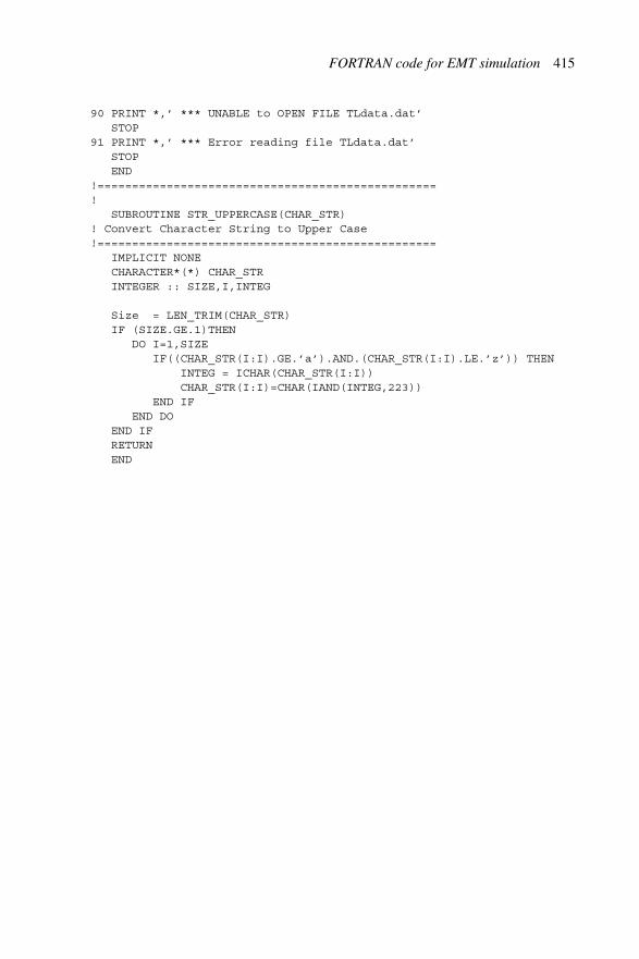
FORTRAN code for EMT simulation 415
90 PRINT *,’ *** UNABLE to OPEN FILE TLdata.dat’STOP
91 PRINT *,’ *** Error reading file TLdata.dat’STOPEND
!=================================================!
SUBROUTINE STR_UPPERCASE(CHAR_STR)! Convert Character String to Upper Case!=================================================
IMPLICIT NONECHARACTER*(*) CHAR_STRINTEGER :: SIZE,I,INTEG
Size = LEN_TRIM(CHAR_STR)IF (SIZE.GE.1)THEN
DO I=1,SIZEIF((CHAR_STR(I:I).GE.’a’).AND.(CHAR_STR(I:I).LE.’z’)) THEN
INTEG = ICHAR(CHAR_STR(I:I))CHAR_STR(I:I)=CHAR(IAND(INTEG,223))
END IFEND DO
END IFRETURNEND


Index
A-stable 357active power (real power) 307, 308admittance matrix 98, 170, 174, 257analogue computer, electronic 4arc resistance 210, 292ARENE 329ATOSEC 8, 37ATP (alternative transient program) 6,
8, 206attenuation of travelling waves 126,
128, 132, 134, 148, 155, 295auto regressive moving average
(ARMA) 30, 148, 267
backward wave 75, 128, 129Bergeron line model 5, 9, 124, 126,
149, 150, 157bilinear transform 6, 28, 100, 369
cable 6, 92, 123, 142, 144, 230, 252,270, 333, 340
capacitance 1, 45, 70, 74, 109, 126,138, 142, 176, 208, 218, 297
Carson’s technique 123, 137, 139, 156characteristic equations 76characteristic impedance 75, 130, 136,
137, 146, 153chatter 82, 97, 217, 220, 222, 227CIGRE HVdc benchmark model 359circuit breaker 3, 9, 54, 194, 210, 230,
321, 326, 334
Clarke transformation 128, 157, 239commutation 222, 236, 248, 287, 289commutation reactance 360companion circuit 6, 69, 78compensation method 89, 212computer systems
graphical interface 7languages 195, 325memory 95, 220software 118, 205, 233, 234, 322,
323, 325, 333conductance matrix 69, 76, 83, 91, 93,
95, 106, 185, 213, 219–221, 224,225, 230, 340, 376
constant current control 55continuous systems 5, 11, 22convergence 21, 43, 44, 60, 244, 248,
279, 285, 286, 356, 357converter 7, 35–37, 44, 49, 53, 55, 94,
194, 217–219, 231–236, 241–248,278–290, 296–304, 313–322,359–365
convolution 21, 114, 130, 132, 134,251, 347, 370
corona losses 140cubic spline interpolation 253current chopping 97, 109, 220, 221,
227, 272, 274curve fitting 254, 313, 348
DFT (Discrete Fourier Transform) 203,255, 260
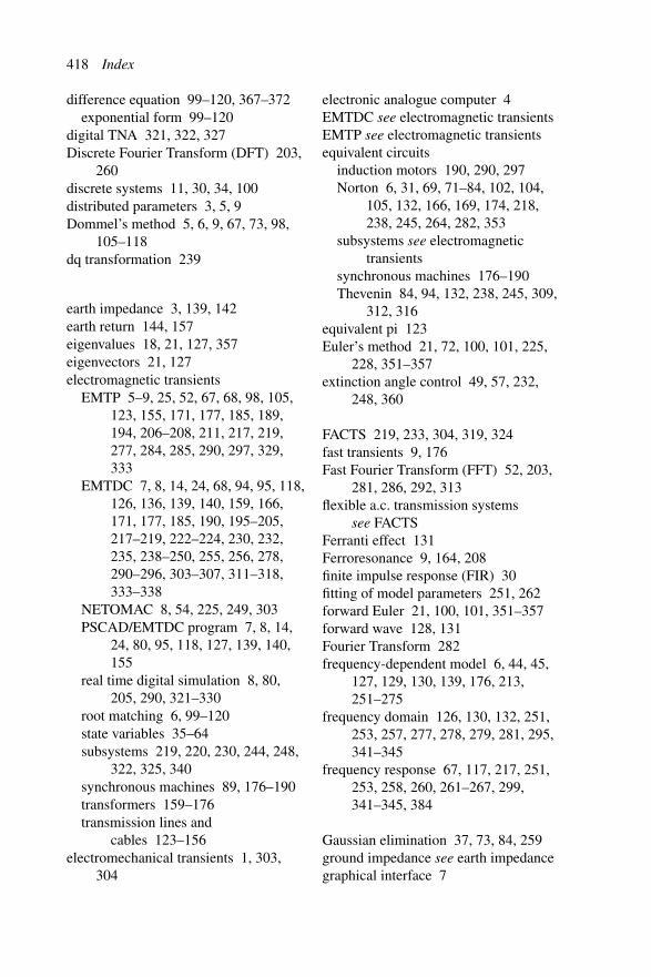
418 Index
difference equation 99–120, 367–372exponential form 99–120
digital TNA 321, 322, 327Discrete Fourier Transform (DFT) 203,
260discrete systems 11, 30, 34, 100distributed parameters 3, 5, 9Dommel’s method 5, 6, 9, 67, 73, 98,
105–118dq transformation 239
earth impedance 3, 139, 142earth return 144, 157eigenvalues 18, 21, 127, 357eigenvectors 21, 127electromagnetic transients
EMTP 5–9, 25, 52, 67, 68, 98, 105,123, 155, 171, 177, 185, 189,194, 206–208, 211, 217, 219,277, 284, 285, 290, 297, 329,333
EMTDC 7, 8, 14, 24, 68, 94, 95, 118,126, 136, 139, 140, 159, 166,171, 177, 185, 190, 195–205,217–219, 222–224, 230, 232,235, 238–250, 255, 256, 278,290–296, 303–307, 311–318,333–338
NETOMAC 8, 54, 225, 249, 303PSCAD/EMTDC program 7, 8, 14,
24, 80, 95, 118, 127, 139, 140,155
real time digital simulation 8, 80,205, 290, 321–330
root matching 6, 99–120state variables 35–64subsystems 219, 220, 230, 244, 248,
322, 325, 340synchronous machines 89, 176–190transformers 159–176transmission lines and
cables 123–156electromechanical transients 1, 303,
304
electronic analogue computer 4EMTDC see electromagnetic transientsEMTP see electromagnetic transientsequivalent circuits
induction motors 190, 290, 297Norton 6, 31, 69, 71–84, 102, 104,
105, 132, 166, 169, 174, 218,238, 245, 264, 282, 353
subsystems see electromagnetictransients
synchronous machines 176–190Thevenin 84, 94, 132, 238, 245, 309,
312, 316equivalent pi 123Euler’s method 21, 72, 100, 101, 225,
228, 351–357extinction angle control 49, 57, 232,
248, 360
FACTS 219, 233, 304, 319, 324fast transients 9, 176Fast Fourier Transform (FFT) 52, 203,
281, 286, 292, 313flexible a.c. transmission systems
see FACTSFerranti effect 131Ferroresonance 9, 164, 208finite impulse response (FIR) 30fitting of model parameters 251, 262forward Euler 21, 100, 101, 351–357forward wave 128, 131Fourier Transform 282frequency-dependent model 6, 44, 45,
127, 129, 130, 139, 176, 213,251–275
frequency domain 126, 130, 132, 251,253, 257, 277, 278, 279, 281, 295,341–345
frequency response 67, 117, 217, 251,253, 258, 260, 261–267, 299,341–345, 384
Gaussian elimination 37, 73, 84, 259ground impedance see earth impedancegraphical interface 7

Index 419
graph method 40GTO 80, 204, 222, 224, 233, 241
harmonics 58, 277, 279, 282, 284, 293,297
HVdc simulator 4high voltage direct current transmission
(HVdc) 230–233, 359a.c.-d.c. converter 230, 313CIGRE benchmark model 234–236,
359simulator 322
history term 26, 31, 69, 75–84, 103,125, 134, 224
homogeneous solution 21, 105hybrid solution 244, 245, 286, 303–308hysteresis 54, 91, 176, 206, 208, 240
ideal switch 115, 219, 339, 376ill-conditioning 70, 162imbalance see unbalanceimplicit integration 22, 44, 71, 100,
101, 351impulse response 21, 23, 30, 94, 133induction machines 190, 290, 297infinite impulse response (IIR) 30inrush current 164insulation co-ordination 1, 3, 9, 211instability 6, 56, 89, 116, 185, 308integration
accuracy 44, 67, 100Adam-Bashforth 352, 353backward Euler 72, 100, 101, 225,
228, 351, 353–357forward Euler 100, 101, 225, 228,
351, 353–357Gear-2nd order 72, 353–357implicit 100, 101predictor-corrector methods 5, 22Runge-Kutta 352stability 356step length 44, 51, 53–64, 85–88,
111, 114, 202, 218, 220, 238,243, 303, 314, 315, 356
trapezoidal 72, 100, 101, 225,353–357
instantaneous term 69, 79, 89, 103, 162interpolation 53, 59, 80, 91, 198, 212,
220–227, 241, 253, 323iterative methods 12, 22, 44, 89, 171,
207, 248, 260, 265, 278
Jacobian matrix 279, 282, 285Jury table 266, 276
Krean 8Kron’s reduction 35, 79
Laplace Transform 11, 17, 20, 33, 133,134
LDU factorisation 230leakage reactance 159, 162, 186, 190,
239, 360lead-lag control 27, 29lower south island (New Zealand) 359LSE (least square error) 253lightning transient 1, 3, 159linear transformation 37loss-free transmission line 73, 76, 123,
124, 147, 148losses 4, 164, 176, 263LTE (local truncation error) 36, 351lumped parameters 4, 245, 289lumped resistance 124
magnetising current 159, 162, 165, 171,284
mapping 100, 220, 285MATLAB 8, 37, 84, 118, 198, 222, 337method of companion circuits 6MicroTran 8modal analysis 11, 21, 123, 126, 131,
137, 340multi-conductor lines 126mutual inductance 160, 178
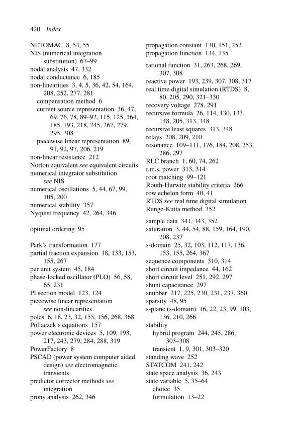
420 Index
NETOMAC 8, 54, 55NIS (numerical integration
substitution) 67–99nodal analysis 47, 332nodal conductance 6, 185non-linearities 3, 4, 5, 36, 42, 54, 164,
208, 252, 277, 281compensation method 6current source representation 36, 47,
69, 76, 78, 89–92, 115, 125, 164,185, 193, 218, 245, 267, 279,295, 308
piecewise linear representation 89,91, 92, 97, 206, 219
non-linear resistance 212Norton equivalent see equivalent circuitsnumerical integrator substitution
see NISnumerical oscillations 5, 44, 67, 99,
105, 200numerical stability 357Nyquist frequency 42, 264, 346
optimal ordering 95
Park’s transformation 177partial fraction expansion 18, 133, 153,
155, 267per unit system 45, 184phase-locked oscillator (PLO) 56, 58,
65, 231PI section model 123, 124piecewise linear representation
see non-linearitiespoles 6, 18, 23, 32, 155, 156, 268, 368Pollaczek’s equations 157power electronic devices 5, 109, 193,
217, 243, 279, 284, 288, 319PowerFactory 8PSCAD (power system computer aided
design) see electromagnetictransients
predictor corrector methods seeintegration
prony analysis 262, 346
propagation constant 130, 151, 252propagation function 134, 135
rational function 31, 263, 268, 269,307, 308
reactive power 193, 239, 307, 308, 317real time digital simulation (RTDS) 8,
80, 205, 290, 321–330recovery voltage 278, 291recursive formula 26, 114, 130, 133,
148, 205, 313, 348recursive least squares 313, 348relays 208, 209, 210resonance 109–111, 176, 184, 208, 253,
286, 297RLC branch 1, 60, 74, 262r.m.s. power 313, 314root matching 99–121Routh-Hurwitz stability criteria 266row echelon form 40, 41RTDS see real time digital simulationRunge-Kutta method 352
sample data 341, 343, 352saturation 3, 44, 54, 88, 159, 164, 190,
208, 237s-domain 25, 32, 103, 112, 117, 136,
153, 155, 264, 367sequence components 310, 314short circuit impedance 44, 162short circuit level 251, 292, 297shunt capacitance 297snubber 217, 225, 230, 231, 237, 360sparsity 48, 95s-plane (s-domain) 16, 22, 23, 99, 103,
136, 210, 266stability
hybrid program 244, 245, 286,303–308
transient 1, 9, 301, 303–320standing wave 252STATCOM 241, 242state space analysis 36, 243state variable 5, 35–64
choice 35formulation 13–22
Index 421
state variable (contd.)valve switching 51
static VAR compensator 233, 236–241step function 105, 356step length 44, 51, 53, 59, 64, 85, 111,
203, 218, 220, 238, 243, 303, 314,315, 356, 357
stiffness 357subsynchronous resonance 9, 184subsystems see electromagnetic
transientssubtransient reactance 186, 289surge arrester 89, 97, 194, 211, 225surge impedance 124, 130, 152swing curves 317switch representation 79switching
chatter 82, 97, 217, 220, 222, 227discontinuities 53, 54, 97, 220, 243,
333Synchronous machine 89, 176–190
excitation 194impedance 310
TACS (transient analysis of controlsystems) 6, 25, 194, 208–213
Taylor’s series 67, 99, 351, 354TCR (thyristor controlled reactor) 233,
236, 240TCS (transient converter
simulation) 44–55automatic time step adjustment 53converter control 55valve switching 51
Thevenin equivalent circuitsee equivalent circuits
three-phase fault 236, 290time constants 3, 22, 49, 84, 105, 136,
184, 278, 303, 357, 360time domain 20, 132, 255, 281, 345time step (step length) see integrationTNA see transient network analysertransfer function 13, 18, 24, 55, 100,
102, 104, 195, 267, 367transformers 159–176
single phase model 166–171three phase model 172–175
transient network analyser 4, 9, 275, 300transient stability 303–319
hybrid program 303–308test system 317
transmission lines 123–142Bergeron model 124–126equivalent pi 123frequency dependent 130–137multi-conductor 126–129
trapezoidal integration see integrationtravelling waves 129, 131
attenuation 132–134velocity of propagation 75
triangular factorization 77, 80, 98truncation errors 6, 36, 97, 99, 351,
354, 356TS see transient stabilityTS/EMTDC interface 307–311
equivalent circuitcomponent 308–310
interface variables derivation 311location 316
Tustin method see bilinear transform
UMEC (unified magnetic equivalentcircuit) 165–172
unbalance 242, 277, 360underground cables 142
valveextinction 49, 53, 232, 248group 56, 230, 232
VAR compensator see static VARcompensator
velocity of wave propagation 75voltage sag 278, 288–292, 300
WLS (weighted least squares) 265
zeros 30, 99, 112, 136, 155, 267, 268zero sequence 130, 171, 186, 239z-plane (z-domain) 22, 32, 99, 101,
116, 199, 266z-transform 31, 276, 345, 346

Neville R. Watson received BE(Hons.) and Ph.D. degrees in 1984 and 1988, respectively, from the University of Canterbury, New Zealand, where he is now a senior lecturer. He is co-author of three other books, has contributed several chapters to a number of edited books and has been published in nearly 120 other publications.Jos Arrillaga received Ph.D. and DSc degrees in 1966 and 1980, respectively, from UMIST, Manchester, UK, where he led the Power Systems Group between 1970 and 1974. Since 1975, he has been a Professor of Electrical Engineering at the University of Canterbury, New Zealand. He is the author of five other books, several book chapters and about 300 other publications. He is a Fellow of the IET, the IEEE and the Academy of Sciences and Royal Society of New Zealand. He was the recipient of the 1997 Uno Lamm medal for his contributions to HVDC transmission.
Power Systems Electromagnetic Transients SimulationAccurate knowledge of electromagnetic power system transients is crucial to the operation of an economic, efficient and environmentally-friendly power system network, without compromising on the reliability and quality of the electrical power supply. Simulation has become a universal tool for the analysis of power system electromagnetic transients and yet is rarely covered in-depth in undergraduate programmes. It is likely to become core material in future courses.
The primary objective of this book is to describe the application of efficient computational techniques to the solution of electromagnetic transient problems in systems of any size and topology, involving linear and non-linear components. The text provides an in-depth knowledge of the different techniques that can be employed to simulate the electromagnetic transients associated with the various components within a power system network, setting up mathematical models and comparing different models for accuracy, computational requirements, etc.
Written primarily for advanced electrical engineering students, the text includes basic examples to clarify difficult concepts. Considering the present lack of training in this area, many practising power engineers, in all aspects of the power industry, will find the book of immense value in their professional work.
The Institution of Engineering and Technologywww.theiet.org 0 85296 106 5978-0-85296-106-3
Related Documents