LECTURE NOTES ON POWER SYSTEM OPERATION AND CONTROL (15A02702) 2018 – 2019 IV B. Tech I Semester (JNTUA-R15) Mr. K.Raju, Assistant Professor CHADALAWADA RAMANAMMA ENGINEERING COLLEGE (AUTONOMOUS) Chadalawada Nagar, Renigunta Road, Tirupati – 517 506 Department of Electrical and Electronics Engineering

Welcome message from author
This document is posted to help you gain knowledge. Please leave a comment to let me know what you think about it! Share it to your friends and learn new things together.
Transcript

LECTURE NOTES
ON
POWER SYSTEM OPERATION
AND CONTROL
(15A02702)
2018 – 2019
IV B. Tech I Semester (JNTUA-R15)
Mr. K.Raju, Assistant Professor
CHADALAWADA RAMANAMMA ENGINEERING COLLEGE (AUTONOMOUS)
Chadalawada Nagar, Renigunta Road, Tirupati – 517 506
Department of Electrical and Electronics Engineering

JAWAHARLAL NEHRU TECHNOLOGICAL UNIVERSITY ANANTAPUR
B. Tech IV-I Sem. (EEE) L T P C
3 1 0 3
15A02702 POWER SYSTEM OPERATION AND CONTROL
Course Objectives: The objectives of the course are to make the students learn about:
Optimum generation allocation
Hydrothermal scheduling
Modeling of turbines and generators
Load frequency control in single area and two area systems
Reactive power compensation in power systems
Power system operation in competitive environment
UNIT – I ECONOMIC OPERATION
Optimal Operation of Thermal Power Units, - Heat Rate Curve – Cost Curve – Incremental Fuel and
Production Costs, Input-Output Characteristics, Optimum Generation Allocation with Line Losses
Neglected. Optimum Generation Allocation Including the Effect of Transmission Line Losses – Loss
Coefficients, General Transmission Line Loss Formula.
UNIT–II HYDROTHERMAL SCHEDULING
Optimal Scheduling of Hydrothermal System: Hydroelectric Power Plant Models, Scheduling Problems-
Short Term Hydrothermal Scheduling Problem. Modeling of Turbine: First Order Turbine Model, Block
Diagram Representation of Steam Turbines and Approximate Linear Models. Modeling of Governor:
Mathematical Modeling of Speed Governing System – Derivation of Small Signal Transfer Function –
Block Diagram.
UNIT – III LOAD FREQUENCY CONTROL
Necessity of Keeping Frequency Constant. Definitions of Control Area – Single Area Control – Block
Diagram Representation of an Isolated Power System – Steady State Analysis – Dynamic Response –
Uncontrolled Case. Load Frequency Control of 2-Area System – Uncontrolled Case and Controlled Case,
Tie-Line Bias Control. Proportional Plus Integral Control of Single Area and Its Block Diagram
Representation, Steady State Response – Load Frequency Control and Economic Dispatch Control.
UNIT – IV REACTIVE POWER CONTROL
Overview of Reactive Power Control – Reactive Power Compensation in Transmission Systems –
Advantages and Disadvantages of Different Types of Compensating Equipment for Transmission Systems;
Load Compensation – Specifications of Load Compensator, Uncompensated and Compensated
Transmission Lines: Shunt and Series Compensation.
UNIT – V POWER SYSTEM OPERATION IN COMPETITIVE ENVIRONMENT
Introduction – Restructuring models – Independent System Operator (ISO) – Power Exchange - Market
operations – Market Power – Standard cost – Transmission Pricing – Congestion Pricing – Management of
Inter zonal/Intra zonal Congestion - Electricity Price Volatility Electricity Price Indexes – Challenges to
Electricity Pricing – Construction of Forward Price Curves – Short-time Price Forecasting

Course Outcomes: After completion of the course, the student will able to:
Develop the mathematical models of turbines and governors
Address the Load Frequency Control problem
Explain how shunt and series compensation helps in reactive power control
Explain the issues concerned with power system operation in competitive environment
TEXT BOOKS:
1. Power System Analysis Operation and Control, Abhijit Chakrabarti and Sunita Halder, PHI Learning Pvt.
Ltd.,, 3rd Edition, 2010.
2. Modern Power System Analysis, D.P.Kothari and I.J.Nagrath, Tata McGraw Hill Publishing Company Ltd., 3rd Edition, 2003, Ninth Reprint 2007.
REFERENCE BOOKS:
1. Power System Analysis and Design, J. Duncan Glover and M.S.Sharma, Thomson, 3rd Edition, 2008.
2. Electric Energy System Theory: An Introduction, Olle Ingemar Elgerd, Tata Mc Graw Hill, 2nd Edition,
1982.
3. Power System Stability and Control, P Kundur, Tata Mc Graw Hill, 1994, 5th Reprint, 2008.

Smartzworld.com Smartworld.asia
jntuworldupdates.org Specworld.in
UNIT-I
ECONOMIC OPERATION
Overview
Economic Distribution of Loads between the Units of a Plant
Generating Limits
Economic Sharing of Loads between Different Plants
Automatic Generation Control
Load Frequency Control
Coordination between LFC and Economic Dispatch
A good business practice is the one in which the production cost is minimized without sacrificing
the quality. This is not any different in the power sector as well. The main aim here is to reduce the
production cost while maintaining the voltage magnitudes at each bus. In this chapter we shall discuss the
economic operation strategy along with the turbine-governor control that are required to maintain the
power dispatch economically.
A power plant has to cater to load conditions all throughout the day, come summer or winter. It is
therefore illogical to assume that the same level of power must be generated at all time. The power
generation must vary according to the load pattern, which may in turn vary with season. Therefore the
economic operation must take into account the load condition at all times. Moreover once the economic
generation condition has been calculated, the turbine-governor must be controlled in such a way that this
generation condition is maintained. In this chapter we shall discuss these two aspects.
Economic operation of power systems
Introduction:
One of the earliest applications of on-line centralized control was to provide a central facility, to
operate economically, several generating plants supplying the loads of the system. Modern integrated
systems have different types of generating plants, such as coal fired thermal plants, hydel plants, nuclear
plants, oil and natural gas units etc. The capital investment, operation and maintenance costs are different
for different types of plants.
The operation economics can again be subdivided into two parts.
i) Problem of economic dispatch, which deals with determining the power output of each plant to meet the
specified load, such that the overall fuel cost is minimized.
ii) Problem of optimal power flow, which deals with minimum – loss delivery, where in the power flow,
is optimized to minimize losses in the system.

Smartzworld.com Smartworld.asia
jntuworldupdates.org Specworld.in
In this chapter we consider the problem of economic dispatch. During operation of the plant, a
generator may be in one of the following states:
i) Base supply without regulation: the output is a constant.
ii) Base supply with regulation: output power is regulated based on system load.
iii) Automatic non-economic regulation: output level changes around a base setting as area control error
changes.
iv) Automatic economic regulation: output level is adjusted, with the area load and area control error,
while tracking an economic setting. Regardless of the units operating state, it has a contribution to the
economic operation, even though its output is changed for different reasons.
The factors influencing the cost of generation are the generator efficiency, fuel cost and
transmission losses. The most efficient generator may not give minimum cost, since it may be located in a
place where fuel cost is high. Further, if the plant is located far from the load centers, transmission losses
may be high and running the plant may become uneconomical. The economic dispatch problem basically
determines the generation of different plants to minimize total operating cost.
Modern generating plants like nuclear plants, geo-thermal plants etc, may require capital investment of
millions of rupees. The economic dispatch is however determined in terms of fuel cost per unit power
generated and does not include capital investment, maintenance, depreciation, start-up and shut down
costs etc.
Performance Curves Input-Output Curve
This is the fundamental curve for a thermal plant and is a plot of the input in British
Thermal units (Btu) per hour versus the power output of the plant in MW as shown in Fig1
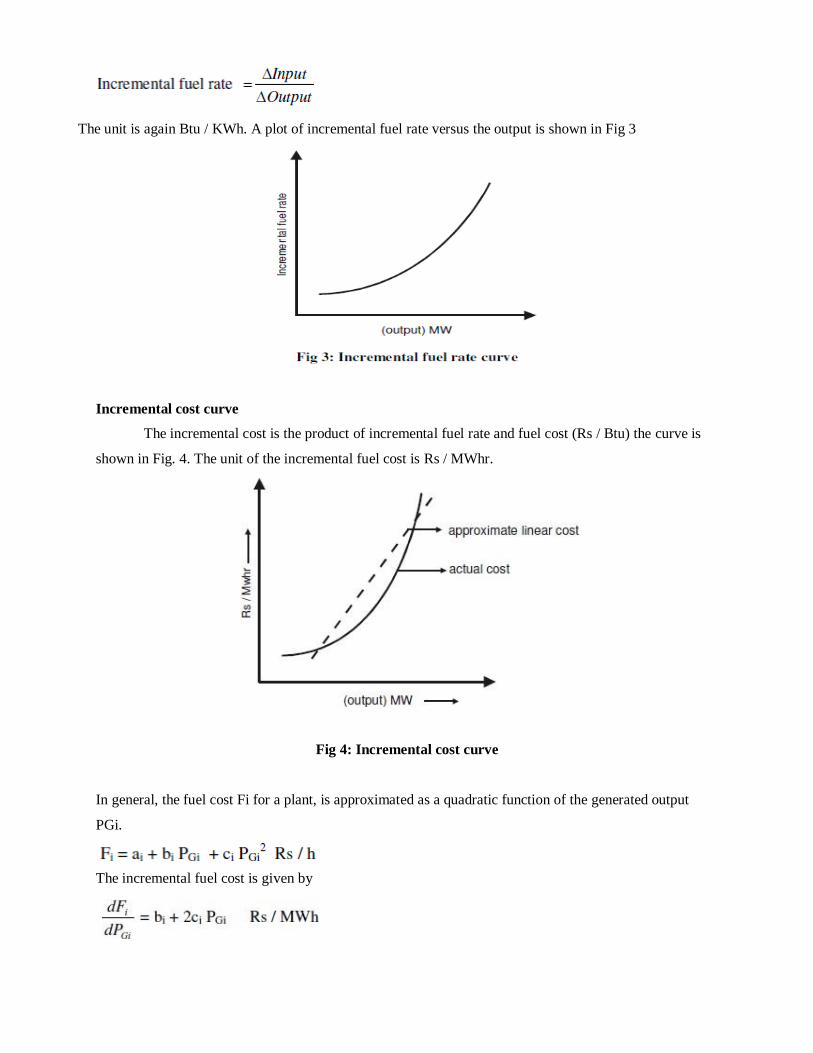
Incremental Fuel Rate Curve
The incremental fuel rate is equal to a small change in input divided by the corresponding change
in output.
Smartzworld.com Smartworld.asia
jntuworldupdates.org Specworld.in
The unit is again Btu / KWh. A plot of incremental fuel rate versus the output is shown in Fig 3
Incremental cost curve
The incremental cost is the product of incremental fuel rate and fuel cost (Rs / Btu) the curve is
shown in Fig. 4. The unit of the incremental fuel cost is Rs / MWhr.
Fig 4: Incremental cost curve
In general, the fuel cost Fi for a plant, is approximated as a quadratic function of the generated output
PGi.
The incremental fuel cost is given by

Smartzworld.com Smartworld.asia
jntuworldupdates.org Specworld.in
Smartzworld.com Smartworld.asia
jntuworldupdates.org Specworld.in
The incremental fuel cost is a measure of how costly it will be produce an increment of power.
The incremental production cost, is made up of incremental fuel cost plus the incremental cost of labor,
water, maintenance etc. which can be taken to be some percentage of the incremental fuel cost, instead of
resorting to a rigorous mathematical model. The cost curve can be approximated by a linear curve. While
there is negligible operating cost for a hydel plant, there is a limitation on the power output possible. In
any plant, all units normally operate between PGmin, the minimum loading limit, below which it is
technically infeasible to operate a unit and PGmax, which is the maximum output limit. Section
I: Economic Operation of Power System
Economic Distribution of Loads between the Units of a Plant
Generating Limits
Economic Sharing of Loads between Different Plants
In an early attempt at economic operation it was decided to supply power from the most efficient
plant at light load conditions. As the load increased, the power was supplied by this most efficient plant
till the point of maximum efficiency of this plant was reached. With further increase in load, the next
most efficient plant would supply power till its maximum efficiency is reached. In this way the power
would be supplied by the most efficient to the least efficient plant to reach the peak demand.
Unfortunately however, this method failed to minimize the total cost of electricity generation. We must
therefore search for alternative method which takes into account the total cost generation of all the units
of a plant that is supplying a load.
Economic Distribution of Loads between the Units of a Plant
To determine the economic distribution of a load amongst the different units of a plant, the
variable operating costs of each unit must be expressed in terms of its power output. The fuel cost is the
main cost in a thermal or nuclear unit. Then the fuel cost must be expressed in terms of the power output.
Other costs, such as the operation and maintenance costs, can also be expressed in terms of the power
output. Fixed costs, such as the capital cost, depreciation etc., are not included in the fuel cost.
The fuel requirement of each generator is given in terms of the Rupees/hour. Let us define the
input cost of an unit- i, fi in Rs/h and the power output of the unit as Pi . Then the input cost can be
expressed in terms of the power output as
Rs/h (1.1)
The operating cost given by the above quadratic equation is obtained by approximating the power
in MW versus the cost in Rupees curve. The incremental operating cost of each unit is then computed as
Rs/MWhr (1.2)

Let us now assume that only two units having different incremental costs supply a load. There
will be a reduction in cost if some amount of load is transferred from the unit with higher incremental cost
to the unit with lower incremental cost. In this fashion, the load is transferred from the less efficient unit
to the more efficient unit thereby reducing the total operation cost. The load transfer will continue till the
incremental costs of both the units are same. This will be optimum point of operation for both the units.
The above principle can be extended to plants with a total of N number of units. The total fuel cost will
then be the summation of the individual
fuel cost fi , i = 1, ... , N of each unit, i.e.,
(1.3)
Let us denote that the total power that the plant is required to supply by PT , such that
(1.4)
Where P1 , ... , PN are the power supplied by the N different units.
The objective is minimizing fT for a given PT. This can be achieved when the total difference dfT becomes
zero, i.e.
(1.5)
Now since the power supplied is assumed to be constant we have
(1.6)
Multiplying (1.6) by λ and subtracting from (1.5) we get
(1.7)
The equality in (5.7) is satisfied when each individual term given in brackets is zero. This gives us
(1.8)
Smartzworld.com Smartworld.asia
jntuworldupdates.org Specworld.in
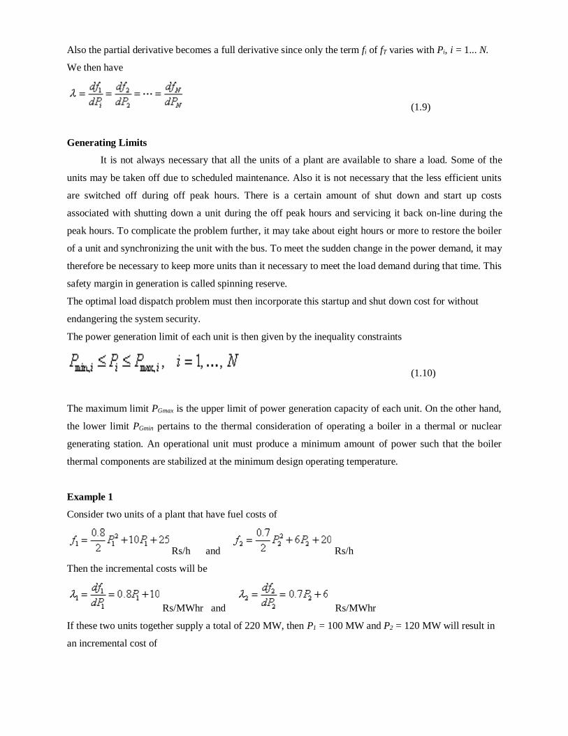
Also the partial derivative becomes a full derivative since only the term fi of fT varies with Pi, i = 1... N.
We then have
(1.9)
Generating Limits
It is not always necessary that all the units of a plant are available to share a load. Some of the
units may be taken off due to scheduled maintenance. Also it is not necessary that the less efficient units
are switched off during off peak hours. There is a certain amount of shut down and start up costs
associated with shutting down a unit during the off peak hours and servicing it back on-line during the
peak hours. To complicate the problem further, it may take about eight hours or more to restore the boiler
of a unit and synchronizing the unit with the bus. To meet the sudden change in the power demand, it may
therefore be necessary to keep more units than it necessary to meet the load demand during that time. This
safety margin in generation is called spinning reserve.
The optimal load dispatch problem must then incorporate this startup and shut down cost for without
endangering the system security.
The power generation limit of each unit is then given by the inequality constraints
(1.10)
The maximum limit PGmax is the upper limit of power generation capacity of each unit. On the other hand,
the lower limit PGmin pertains to the thermal consideration of operating a boiler in a thermal or nuclear
generating station. An operational unit must produce a minimum amount of power such that the boiler
thermal components are stabilized at the minimum design operating temperature.
Example 1
Consider two units of a plant that have fuel costs of
Rs/h and Rs/h
Then the incremental costs will be
Rs/MWhr and Rs/MWhr
If these two units together supply a total of 220 MW, then P1 = 100 MW and P2 = 120 MW will result in
an incremental cost of

Smartzworld.com Smartworld.asia
jntuworldupdates.org Specworld.in
Rs/MWhr and Rs/MWhr
This implies that the incremental costs of both the units will be same, i.e., the cost of one extra MW of
generation will be Rs. 90/MWhr. Then we have
Rs/h and Rs/h
And total cost of generation is p
Rs/h
Now assume that we operate instead with P 1 = 90 MW and P 2 = 130 MW. Then the individual cost of
each unit will be
Rs/h and Rs/h
And total cost of generation is
Rs./h
This implies that an additional cost of Rs. 75 is incurred for each hour of operation with this non-optimal
setting. Similarly it can be shown that the load is shared equally by the two units, i.e. P1 = P2 = 110 MW,
then the total cost is again 10,880 Rs/h.
Example 2
Let us consider a generating station that contains a total number of three generating units. The fuel costs
of these units are given by
Rs/h
Rs/h
Rs/h
The generation limits of the units are
The total load that these units supply varies between 90 MW and 1250 MW. Assuming that all the three
units are operational all the time, we have to compute the economic operating settings as the load
changes.

Smartzworld.com Smartworld.asia
jntuworldupdates.org Specworld.in
The incremental costs of these units are
Rs/MWhr
Rs/MWhr
Rs/MWhr
At the minimum load the incremental cost of the units are
Rs/MWhr
Rs/MWhr
Rs/MWhr
Since units 1 and 3 have higher incremental cost, they must therefore operate at 30 MW each. The
incremental cost during this time will be due to unit-2 and will be equal to 26 Rs/MWhr. With the
generation of units 1 and 3 remaining constant, the generation of unit-2 is increased till its incremental
cost is equal to that of unit-1, i.e., 34 Rs/MWhr. This is achieved when P2 is equal to 41.4286 MW, at a
total power of 101.4286 MW.
An increase in the total load beyond 101.4286 MW is shared between units 1 and 2, till their incremental
costs are equal to that of unit-3, i.e., 43.5 Rs/MWhr. This point is reached when P1 = 41.875 MW and P2
= 55 MW. The total load that can be supplied at that point is equal to 126.875. From this point onwards
the load is shared between the three units in such a way that the incremental costs of all the units are
same. For example for a total load of 200 MW, from (5.4) and (5.9) we have
Solving the above three equations we get P1 = 66.37 MW, P2 = 80 MW and P3 = 50.63 MW and an
incremental cost (λ) of 63.1 Rs./MWhr. In a similar way the economic dispatch for various other load
settings are computed. The load distribution and the incremental costs are listed in Table 5.1 for various
total power conditions.

Smartzworld.com Smartworld.asia
jntuworldupdates.org Specworld.in
At a total load of 906.6964, unit-3 reaches its maximum load of 250 MW. From this point onwards then,
the generation of this unit is kept fixed and the economic dispatch problem involves the other two units.
For example for a total load of 1000 MW, we get the following two equations from (1.4) and (1.9)
Solving which we get P1 = 346.67 MW and P2 = 403.33 MW and an incremental cost of 287.33
Rs/MWhr. Furthermore, unit-2 reaches its peak output at a total load of 1181.25. Therefore any further
increase in the total load must be supplied by unit-1 and the incremental cost will only be borne by this
unit. The power distribution curve is shown in Fig. 5.
Fig5. Power distribution between the units of Example 2
Example 3
Consider two generating plant with same fuel cost and generation limits. These are given by
For a particular time of a year, the total load in a day varies as shown in Fig. 5.2. Also an additional cost
of Rs. 5,000 is incurred by switching of a unit during the off peak hours and switching it back on during
the during the peak hours. We have to determine whether it is economical to have both units operational
all the time.

Smartzworld.com Smartworld.asia
jntuworldupdates.org Specworld.in
Fig.6. Hourly distribution of a load for the units of Example 2
Since both the units have identical fuel costs, we can switch of any one of the two units during the off
peak hour. Therefore the cost of running one unit from midnight to 9 in the morning while delivering 200
MW is
Rs.
Adding the cost of Rs. 5,000 for decommissioning and commissioning the other unit after nine hours, the
total cost becomes Rs. 167,225. 0
On the other hand, if both the units operate all through the off peak hours sharing power equally, then we
get a total cost of
Rs.
Which is significantly less that the cost of running one unit alone?
Table 1.1 Load distribution and incremental cost for the units of Example 1
PT (MW) P1 (MW) P2 (MW) P3 (MW) λ (Rs./MWh)
90 30 30 30 26
101.4286 30 41.4286 30 34
120 38.67 51.33 30 40.93
126.875 41.875 55 30 43.5
150 49.62 63.85 36.53 49.7
200 66.37 83 50.63 63.1
300 99.87 121.28 78.85 89.9
400 133.38 159.57 107.05 116.7
500 166.88 197.86 135.26 143.5
Smartzworld.com Smartworld.asia
jntuworldupdates.org Specworld.in
600 200.38 236.15 163.47 170.3
700 233.88 274.43 191.69 197.1
800 267.38 312.72 219.9 223.9
906.6964 303.125 353.5714 250 252.5
1000 346.67 403.33 250 287.33
1100 393.33 456.67 250 324.67
1181.25 431.25 500 250 355
1200 450 500 250 370
1250 500 500 250 410
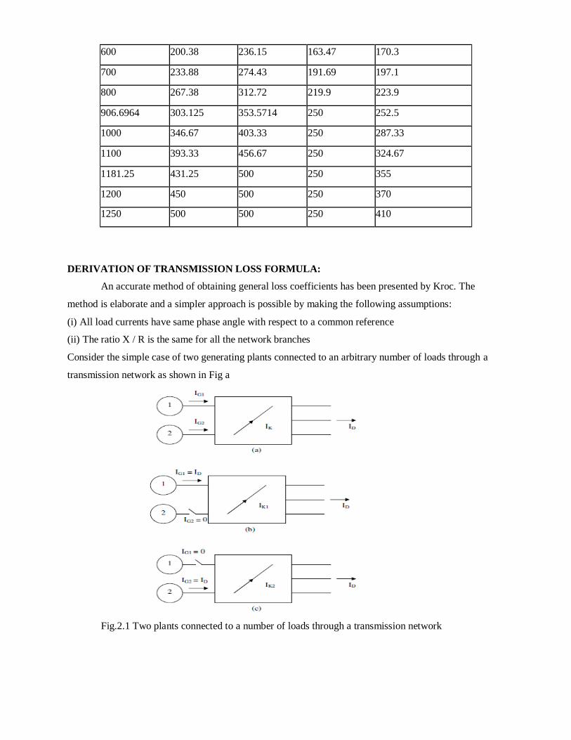
DERIVATION OF TRANSMISSION LOSS FORMULA:
An accurate method of obtaining general loss coefficients has been presented by Kroc. The
method is elaborate and a simpler approach is possible by making the following assumptions:
(i) All load currents have same phase angle with respect to a common reference
(ii) The ratio X / R is the same for all the network branches
Consider the simple case of two generating plants connected to an arbitrary number of loads through a
transmission network as shown in Fig a
Fig.2.1 Two plants connected to a number of loads through a transmission network

Smartzworld.com Smartworld.asia
jntuworldupdates.org Specworld.in
Let‟s assume that the total load is supplied by only generator 1 as shown in Fig 8.9b. Let the current
through a branch K in the network be IK1. We define
It is to be noted that IG1 = ID in this case. Similarly with only plant 2 supplying the load
Current ID, as shown in Fig 8.9c, we define
NK1 and NK2 are called current distribution factors and their values depend on the impedances of the
lines and the network connection. They are independent of ID. When both generators are supplying the
load, then by principle of superposition IK = NK1 IG1 + NK2 IG2
Where IG1, IG2 are the currents supplied by plants 1 and 2 respectively, to meet the demand ID. Because
of the assumptions made, IK1 and ID have same phase angle, as do IK2 and ID. Therefore, the current
distribution factors are real rather than complex. Let
Where σ1 and σ2 are phase angles of IG1 and IG2 with respect to a common reference. We can write
Where PG1, PG2 are three phase real power outputs of plant1 and plant 2; V1, V2 are the line to line bus
voltages of the plants and Φ1 and Φ2 are the power factor angles.
The total transmission loss in the system is given by
Where the summation is taken over all branches of the network and RK is the branch
resistance. Substituting we get

Smartzworld.com Smartworld.asia
jntuworldupdates.org Specworld.in
The loss – coefficients are called the B – coefficients and have unit MW-1
For a general system with n plants the transmission loss is expressed as
In a compact form
B – Coefficients can be treated as constants over the load cycle by computing them at average operating
conditions, without significant loss of accuracy.
Economic Sharing of Loads between Different Plants
So far we have considered the economic operation of a single plant in which we have discussed
how a particular amount of load is shared between the different units of a plant. In this problem we did
not have to consider the transmission line losses and assumed that the losses were a part of the load
supplied. However if now consider how a load is distributed between the different plants that are joined

Smartzworld.com Smartworld.asia
jntuworldupdates.org Specworld.in
by transmission lines, then the line losses have to be explicitly included in the economic dispatch
problem. In this section we shall discuss this problem.
When the transmission losses are included in the economic dispatch problem
(2.1)
(2.2)
Where PLOSS is the total line loss. Since PT is assumed to be constant, we have
................ (2.3)
In the above equation dPLOSS includes the power loss due to every generator, i.e.,
Also minimum generation cost implies dfT = 0 as given in (1.5). Multiplying both (2.2) and (2.3) by λ and
combining we get
(2.4)
(2.5)
Adding (2.4) with (1.5) we obtain
The above equation satisfies when
Again since
(2.6)
(2.7)
From (2.6) we get
(2.8)
Where Li is called the penalty factor of load- i and is given by

Smartzworld.com Smartworld.asia
jntuworldupdates.org Specworld.in
Consider an area with N number of units. The power generated are defined by the vector
(2.9)
Then the transmission losses are expressed in general as
Where B is a symmetric matrix given by
The elements Bij of the matrix B are called the loss coefficients. These coefficients are not constant but
vary with plant loading. However for the simplified calculation of the penalty factor Li these coefficients
are often assumed to be constant.
When the incremental cost equations are linear, we can use analytical equations to find out the economic
settings. However in practice, the incremental costs are given by nonlinear equations that may even
contain nonlinearities. In that case iterative solutions are required to find the optimal generator settings.

Smartzworld.com Smartworld.asia
jntuworldupdates.org Specworld.in
UNIT-II
HYDROTHERMAL SCHEDULING
Long-Range Hydro-Scheduling:
The long-range hydro-scheduling problem involves the long-range forecasting of water availability
and the scheduling of reservoir water releases (i.e., “drawdown”) for an interval of time that depends on
the reservoir capacities. Typical long range scheduling goes anywhere from 1 wk to 1 yr or several years.
For hydro schemes with a capacity of impounding water over several seasons, the long-range problem
involves meteorological and statistical analyses.
Short-Range Hydro-Scheduling
Short-range hydro-scheduling (1 day to I wk) involves the hour-by-hour scheduling of all generation
on a system to achieve minimum production cost for the given time period. In such a scheduling problem,
the load, hydraulic inflows, and unit availabilities are assumed known. A set of starting conditions (e.g.,
reservoir levels) is given, and the optimal hourly schedule that minimizes a desired objective, while
meeting hydraulic steam, and electric system constraints, is sought.
Hydrothermal systems where the hydroelectric system is by far the largest component may be
scheduled by economically scheduling the system to produce the minimum cost for the thermal system.
The schedules are usually developed to minimize thermal generation production costs, recognizing all the
diverse hydraulic constraints that may exist
2.8 OPTIMAL POWER FLOW PROBLEM: Basic approach to the solution of this problem is to
incorporate the power flow equations as essential constraints in the formal establishment of the
optimization problem. This general approach is known as the optimal power flow. Another approach is by
using loss-formula method. Different techniques are: 1) the lambda-iteration method 2) Gradient methods
of economic dispatch 3) Newton's method 4) Economic dispatch with piecewise linear cost functions 5)
Economic dispatch using dynamic programming
Smartzworld.com Smartworld.asia
Smartworld.asia
jntuworldupdates.org Specworld.in
Smartzworld.com Smartworld.asia
jntuworldupdates.org Specworld.in
The main objective of power system operation and control is to maintain continuous supply of power
with an acceptable quality, to all the consumers in the system. The system will be in equilibrium, when
there is a balance between the power demand and the power generated. As the power in AC form has real
and reactive components: the real power balance; as well as the reactive power balance is to be achieved.
There are two basic control mechanisms used to achieve reactive power balance (acceptable voltage
profile) and real power balance (acceptable frequency values). The former is called the automatic voltage
regulator (AVR) and the latter is called the automatic load frequency control (ALFC) or automatic
generation control (AGC).
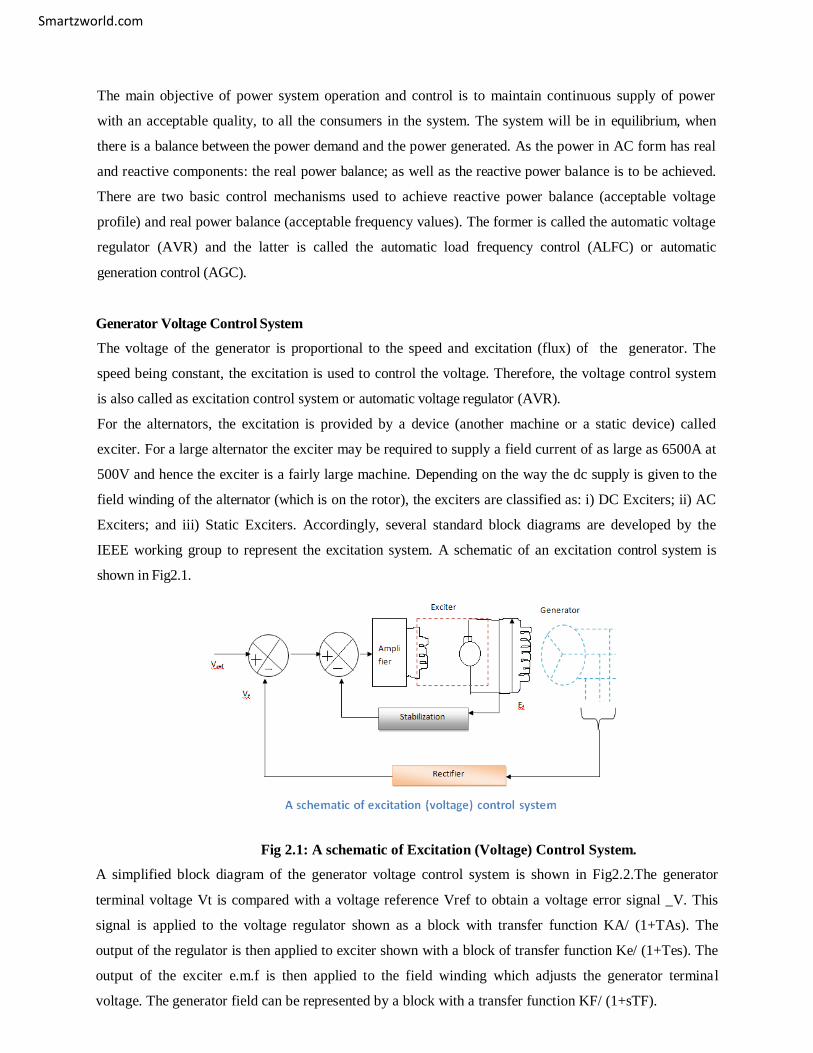
Generator Voltage Control System
The voltage of the generator is proportional to the speed and excitation (flux) of the generator. The
speed being constant, the excitation is used to control the voltage. Therefore, the voltage control system
is also called as excitation control system or automatic voltage regulator (AVR).
For the alternators, the excitation is provided by a device (another machine or a static device) called
exciter. For a large alternator the exciter may be required to supply a field current of as large as 6500A at
500V and hence the exciter is a fairly large machine. Depending on the way the dc supply is given to the
field winding of the alternator (which is on the rotor), the exciters are classified as: i) DC Exciters; ii) AC
Exciters; and iii) Static Exciters. Accordingly, several standard block diagrams are developed by the
IEEE working group to represent the excitation system. A schematic of an excitation control system is
shown in Fig2.1.
Fig 2.1: A schematic of Excitation (Voltage) Control System.
A simplified block diagram of the generator voltage control system is shown in Fig2.2.The generator
terminal voltage Vt is compared with a voltage reference Vref to obtain a voltage error signal _V. This
signal is applied to the voltage regulator shown as a block with transfer function KA/ (1+TAs). The
output of the regulator is then applied to exciter shown with a block of transfer function Ke/ (1+Tes). The
output of the exciter e.m.f is then applied to the field winding which adjusts the generator terminal
voltage. The generator field can be represented by a block with a transfer function KF/ (1+sTF).

Smartzworld.com Smartworld.asia
Smartzworld.com Smartworld.asia
jntuworldupdates.org Specworld.in
The total
transfer function is
The stabilizing compensator shown in the diagram is used to improve the dynamic response of the exciter.
The input to this block is the exciter voltage and the output is a stabilizing feedback signal to reduce the
excessive overshoot.
Fig2.2: A simplified block diagram of Voltage (Excitation) Control System.
Performance of AVR Loop
The purpose of the AVR loop is to maintain the generator terminal voltage with inacceptable values. A
static accuracy limit in percentage is specified for the AVR, so that the terminal voltage is maintained
within that value. For example, if the accuracy limit is 4%, then the terminal voltage must be maintained
within 4% of the base voltage.
The performance of the AVR loop is measured by its ability to regulate the terminal voltage of the
generator within prescribed static accuracy limit with an acceptable speed of response. Suppose the static
accuracy limit is denoted by Ac in percentage with reference to the nominal value. The error voltage is to
be less than (Ac/100) |Vref. From the block diagram, for a steady state error voltage

Smartzworld.com Smartworld.asia
jntuworldupdates.org Specworld.in
For constant input condition, (s0)
Where, K= G(0) is the open loop gain of the AVR. Hence,
Automatic Load Frequency Control
The ALFC is to control the frequency deviation by maintaining the real power balance in the system. The
main functions of the ALFC are to i) to maintain the steady frequency; ii) control the tie-line flows; and
iii) distribute the load among the participating generating units. The control (input) signals are the tie-line
deviation ∆Ptie (measured from the tie line flows), and the frequency deviation ∆f (obtained by measuring
the angle deviation ∆δ). These error signals ∆f and ∆Ptie are amplified, mixed and transformed to a real
power signal, which then controls the valve position. Depending on the valve position, the turbine (prime mover) changes its output power to establish the real power balance. The complete control schematic is shown
in Fig2.3
Fig2.3.The Schematic representation of ALFC system
For the analysis, the models for each of the blocks in Fig2 are required. The generator and the electrical
load constitute the power system. The valve and the hydraulic amplifier represent the speed governing
system. Using the swing equation, the generator can be modeled by

Smartzworld.com Smartworld.asia
jntuworldupdates.org Specworld.in
Expressing the speed deviation in pu,
This relation can be represented as shown in Fig2.4.
Fig2.4.The block diagram representation of the Generator
Fig2.5.The block diagram representation of the Generator and load
The turbine can be modeled as a first order lag as shown in the Fig2.6
Fig2.6.The turbine model
Gt(s) is the TF of the turbine; ∆PV(s) is the change in valve output (due to action).
∆Pm(s) is the change in the turbine output the governor can similarly modeled as shown in Fig2.7. The
output of the governor is by

Smartworld.asia
Smartzworld.com
jntuworldupdates.org Specworld.in
Fig2.7: The block diagram representation of the Governor
All the individual blocks can now be connected to represent the complete ALFC loop as
Shown in Fig 5.1
Fig2.8: The block diagram representation of the ALFC.
2.2 Steady state Performance of the ALFC Loop:
In the steady state, the ALFC is in „open‟ state, and the output is obtained by substituting
S → 0 in the TF.
With S → 0,

Smartzworld.com Smartworld.asia
jntuworldupdates.org Specworld.in
supplementary controls); ii) and to maintain the scheduled tie-line flows. A secondary objective of the

Smartzworld.com Smartworld.asia
jntuworldupdates.org Specworld.in
AGC is to distribute the required change in generation among the connected generating units
economically (to obtain least operating costs).
Fig2.9: The block diagram representation of the AGC

Smartzworld.com Smartworld.asia
jntuworldupdates.org Specworld.in
Fig.2.10.AGC for a multi-area operation

jntuworldupdates.org Specworld.in
Smartzworld.com Smartworld.asia
• Net interchange power (tie line flow) with neighboring areas at the scheduled
Values
Smartzworld.com
Smartworld.asia
jntuworldupdates.org Specworld.in
The supplementary control should ideally correct only for changes in that area. In other words, if there is
a change in Area1 load, there should be supplementary control only in Area1 and not in Area 2. For this
purpose the area control error (ACE) is used (Fig2.9). The ACE of the two areas are given by
Economic Allocation of Generation
An important secondary function of the AGC is to allocate generation so that each generating unit is
loaded economically. That is, each generating unit is to generate that amount to meet the present demand
in such a way that the operating cost is the minimum. This function is called Economic Load Dispatch
(ELD).
Systems with more than two areas
The method described for the frequency bias control for two area system is applicable to multiage system
also.
Section II: Automatic Generation Control
Load Frequency Control
Automatic Generation Control
Electric power is generated by converting mechanical energy into electrical energy. The rotor mass,
which contains turbine and generator units, stores kinetic energy due to its rotation. This stored kinetic
energy accounts for sudden increase in the load. Let us denote the mechanical torque input by Tm and the
output electrical torque by Te . Neglecting the rotational losses, a generator unit is said to be operating in
the steady state at a constant speed when the difference between these two elements of torque is zero. In
this case we say that the accelerating torque is zero.
5.20)
When the electric power demand increases suddenly, the electric torque increases. However, without any
feedback mechanism to alter the mechanical torque, Tm remains constant. Therefore the accelerating
torque given by (5.20) becomes negative causing a deceleration of the rotor mass. As the rotor
decelerates, kinetic energy is released to supply the increase in the load. Also note that during this time,
the system frequency, which is proportional to the rotor speed, also decreases. We can thus infer that any
deviation in the frequency for its nominal value of 50 or 60 Hz is indicative of the imbalance between Tm
and Te. The frequency drops when Tm < Te and rises when Tm > Te .

Smartzworld.com
jntuworldupdates.org Specworld.in
Smartworld.asia
The steady state power-frequency relation is shown in Fig. 5.3. In this figure the slope of the ΔPref line is
negative and is given by
(5.21)
Where R is called the regulating constant. From this figure we can write the steady state power
frequency relation as
Fig. 5.3 A typical steady-state power-frequency curve.
(5.22)
Suppose an interconnected power system contains N turbine-generator units. Then the steady-state power
frequency relation is given by the summation of (5.22) for each of these units as
(5.23)
In the above equation, ΔPm is the total change in turbine-generator mechanical power and ΔPref is the total
change in the reference power settings in the power system. Also note that since all the generators are
supposed to work in synchronism, the change is frequency of each of the units is the same and is denoted
by Δf. Then the frequency response characteristics is defined as
(5.24)
Smartzworld.com Smartworld.asia
jntuworldupdates.org Specworld.in
We can therefore modify (5.23) as
(5.25)
Example 5.5
Consider an interconnected 50-Hz power system that contains four turbine-generator units rated 750 MW,
500 MW, 220 MW and 110 MW. The regulating constant of each unit is 0.05 per unit based on its own
rating. Each unit is operating on 75% of its own rating when the load is suddenly dropped by 250 MW.
We shall choose a common base of 500 MW and calculate the rise in frequency and drop in the
mechanical power output of each unit.
The first step in the process is to convert the regulating constant, which is given in per unit in the base of
each generator, to a common base. This is given as
(5.26)
We can therefore write
Therefore
Per unit
We can therefore calculate the total change in the frequency from (5.25) while assuming ΔPref = 0, i.e., for
no change in the reference setting. Since the per unit change in load - 250/500 = - 0.5 with the negative
sign accounting for load reduction, the change in frequency is given by
Then the change in the mechanical power of each unit is calculated from (5.22) as

Smartzworld.com Smartworld.asia
jntuworldupdates.org Specworld.in
It is to be noted that once ΔPm2 is calculated to be - 79.11 MW, we can also calculate the changes in the
mechanical power of the other turbine-generators units as
This implies that each turbine-generator unit shares the load change in accordance with its own rating.
Smartzworld.com Smartworld.asia
jntuworldupdates.org Specworld.in
UNIT - III
LOAD FREQUENCY CONTROL
Modern day power systems are divided into various areas. For example in India, there are five
regional grids, e.g., Eastern Region, Western Region etc. Each of these areas is generally interconnected
to its neighboring areas. The transmission lines that connect an area to its neighboring area are called tie-
lines. Power sharing between two areas occurs through these tie-lines. Load frequency control, as the
name signifies, regulates the power flow between different areas while holding the frequency constant.
As we have an Example 5.5 that the system frequency rises when the load decreases if ΔPref is kept at
zero. Similarly the frequency may drop if the load increases. However it is desirable to maintain the
frequency constant such that Δf=0. The power flow through different tie-lines are scheduled - for
example, area- i may export a pre-specified amount of power to area- j while importing another pre-
specified amount of power from area- k . However it is expected that to fulfill this obligation, area- i
absorbs its own load change, i.e., increase generation to supply extra load in the area or decrease
generation when the load demand in the area has reduced. While doing this area- i must however maintain
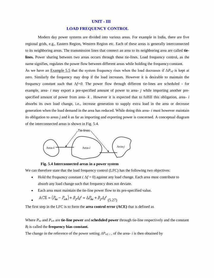
its obligation to areas j and k as far as importing and exporting power is concerned. A conceptual diagram
of the interconnected areas is shown in Fig. 5.4.
Fig. 5.4 Interconnected areas in a power system
We can therefore state that the load frequency control (LFC) has the following two objectives:
Hold the frequency constant ( Δf = 0) against any load change. Each area must contribute to
absorb any load change such that frequency does not deviate.
Each area must maintain the tie-line power flow to its pre-specified value.
(5.27)
The first step in the LFC is to form the area control error (ACE) that is defined as
Where Ptie and Psch are tie-line power and scheduled power through tie-line respectively and the constant
Bf is called the frequency bias constant.
The change in the reference of the power setting ΔPref, i , of the area- i is then obtained by

Smartzworld.com Smartworld.asia
jntuworldupdates.org Specworld.in
(5.28)
The feedback of the ACE through an integral controller of the form where Ki is the integral gain. The
ACE is negative if the net power flow out of an area is low or if the frequency has dropped or both. In this
case the generation must be increased. This can be achieved by increasing ΔPref, i . This negative sign
accounts for this inverse relation between ΔPref, i and ACE. The tie-line power flow and frequency of each
area are monitored in its control center. Once the ACE is computed and ΔPref, i is obtained from (5.28),
commands are given to various turbine-generator controls to adjust their reference power settings.
Example 5.6
Consider a two-area power system in which area-1 generates a total of 2500 MW, while area-2 generates
2000 MW. Area-1 supplies 200 MW to area-2 through the inter-tie lines connected between the two areas.
The bias constant of area-1 ( β1 ) is 875 MW/Hz and that of area-2 ( β2 ) is 700 MW/Hz. With the two
areas operating in the steady state, the load of area-2 suddenly increases by 100 MW. It is desirable that
area-2 absorbs its own load change while not allowing the frequency to drift.
The area control errors of the two areas are given by
And
Since the net change in the power flow through tie-lines connecting these two areas must be zero, we
have
Also as the transients die out, the drift in the frequency of both these areas is assumed to be constant, i.e.
If the load frequency controller (5.28) is able to set the power reference of area-2 properly, the ACE of
the two areas will be zero, i.e., ACE1 = ACE2 = 0. Then we have
This will imply that Δf will be equal to zero while maintaining ΔPtie1 =ΔPtie2 = 0. This signifies that area-2
picks up the additional load in the steady state.
Coordination between LFC and Economic Dispatch
Both the load frequency control and the economic dispatch issue commands to change the power setting
of each turbine-governor unit. At a first glance it may seem that these two commands can be conflicting.
This however is not true. A typical automatic generation control strategy is shown in Fig. 5.5 in which
both the objective are coordinated. First we compute the area control error. A share of this ACE,
proportional to αi , is allocated to each of the turbine-generator unit of an area. Also the share of unit- i , γi
X Σ( PDK - Pk ), for the deviation of total generation from actual generation is computed. Also the error

Smartzworld.com Smartworld.asia
jntuworldupdates.org Specworld.in
between the economic power setting and actual power setting of unit- i is computed. All these signals are
then combined and passed through a proportional gain Ki to obtain the turbine-governor control signal.
Fig. 5.5 Automatic generation control of unit-i
Section II: Swing Equation
Let us consider a three-phase synchronous alternator that is driven by a prime mover. The equation of
motion of the machine rotor is given by
Where
J is the total moment of inertia of the rotor mass in kgm2
Tm is the mechanical torque supplied by the prime mover in N-m
Te is the electrical torque output of the alternator in N-m
θ is the angular position of the rotor in rad
Neglecting the losses, the difference between the mechanical and electrical torque gives the net
accelerating torque Ta . In the steady state, the electrical torque is equal to the mechanical torque, and
hence the accelerating power will be zero. During this period the rotor will move at synchronous speed
ωs in rad/s.
The angular position θ is measured with a stationary reference frame. To represent it with respect to the
synchronously rotating frame, we define
(9.7)
Where δ is the angular position in radians with respect to the synchronously rotating

Smartzworld.com Smartworld.asia
jntuworldupdates.org Specworld.in
(9.8)
Reference frame. Taking the time derivative of the above equation we get
Defining the angular speed of the rotor as
We can write (9.8) as
(9.9)
We can therefore conclude that the rotor angular speed is equal to the synchronous speed only when dδ /
dt is equal to zero. We can therefore term dδ /dt as the error in speed.
(9.10)
Taking derivative of (9.8), we can then rewrite (9.6) as Multiplying both side of (9.11) by ωm we get
(9.11)
Where Pm , Pe and Pa respectively are the mechanical, electrical and accelerating power in MW.
(9.12)
We now define a normalized inertia constant as Substituting (9.12) in (9.10) we get
(9.13)
In steady state, the machine angular speed is equal to the synchronous speed and hence we can replace ωr
in the above equation by ωs. Note that in (9.13) Pm , Pe and Pa are given in MW. Therefore dividing them
by the generator MVA rating Srated we can get these quantities in per unit. Hence dividing both sides of
(9.13) by Srated we get
per unit (9.14)

Smartzworld.com
Smartworld.asia
jntuworldupdates.org Specworld.in
Equation (9.14) describes the behavior of the rotor dynamics and hence is known as the swing equation.
The angle δ is the angle of the internal emf of the generator and it dictates the amount of power that can
be transferred. This angle is therefore called the load angle.
Example 9.2
A 50 Hz, 4-pole turbo generator is rated 500 MVA, 22 kV and has an inertia constant (H) of 7.5. Assume
that the generator is synchronized with a large power system and has a zero accelerating power while
delivering a power of 450 MW. Suddenly its input power is changed to 475 MW. We have to find the
speed of the generator in rpm at the end of a period of 10 cycles. The rotational losses are assumed to be
zero.
We then have
Noting that the generator has four poles, we can rewrite the above equation as
The machines accelerates for 10 cycles, i.e., 20 × 10 = 200 ms = 0.2 s, starting with a synchronous speed
of 1500 rpm. Therefore at the end of 10 cycles
Speed = 1500 + 43.6332 ́0.2 = 1508.7266 rpm.

Smartzworld.com
Smartworld.asia
jntuworldupdates.org Specworld.in
UNIT- IV
REACTIVE POWER CONTROL
Compensation of Power Transmission Systems
Introduction
Ideal Series Compensator
Impact of Series Compensator on Voltage Profile
Improving Power-Angle Characteristics
An Alternate Method of Voltage Injection
Improving Stability Margin
Comparisons of the Two Modes of Operation
Power Flow Control and Power Swing Damping
Introduction
The two major problems that the modern power systems are facing are voltage and angle stabilities. There
are various approaches to overcome the problem of stability arising due to small signal oscillations in an
interconnected power system. As mentioned in the previous chapter, installing power system stabilizers
with generator excitation control system provides damping to these oscillations. However, with the
advancement in the power electronic technology, various reactive power control equipment are
increasingly used in power transmission systems.
A power network is mostly reactive. A synchronous generator usually generates active power that is
specified by the mechanical power input. The reactive power supplied by the generator is dictated by the
network and load requirements. A generator usually does not have any control over it. However the lack
of reactive power can cause voltage collapse in a system. It is therefore important to supply/absorb excess
reactive power to/from the network. Shunt compensation is one possible approach of providing reactive
power support.
A device that is connected in parallel with a transmission line is called a shunt compensator, while a
device that is connected in series with the transmission line is called a series compensator. These are
referred to as compensators since they compensate for the reactive power in the ac system. We shall
assume that the shunt compensator is always connected at the midpoint of transmission system, while the
voltage profile
power-angle characteristics
stability margin
damping to power oscillations

Smartzworld.com Smartworld.asia
jntuworldupdates.org Specworld.in
A static var compensator (SVC) is the first generation shunt compensator. It has been around
since 1960s. In the beginning it was used for load compensation such as to provide var support
for large industrial loads, for flicker mitigation etc. However with the advancement of
semiconductor technology, the SVC started appearing in the transmission systems in 1970s.
Today a large number of SVCs are connected to many transmission systems all over the world.
An SVC is constructed using the thyristors technology and therefore does not have gate turn off
capability.
With the advancement in the power electronic technology, the application of a gate turn off
thyristors (GTO) to high power application became commercially feasible. With this the second
generation shunt compensator device was conceptualized and constructed. These devices use
synchronous voltage sources for generating or absorbing reactive power. A synchronous voltage
source (SVS) is constructed using a voltage source converter (VSC). Such a shunt compensating
device is called static compensator or STATCOM. A STATCOM usually contains an SVS that
is driven from a dc storage capacitor and the SVS is connected to the ac system bus through an
interface transformer. The transformer steps the ac system voltage down such that the voltage
rating of the SVS switches are within specified limit. Furthermore, the leakage reactance of the
transformer plays a very significant role in the operation of the STATCOM.
Like the SVC, a thyristors controlled series compensator (TCSC) is a thyristors based series
compensator that connects a thyristors controlled reactor ( TCR ) in parallel with a fixed
capacitor. By varying the firing angle of the anti-parallel thyristors that are connected in series
with a reactor in the TCR, the fundamental frequency inductive reactance of the TCR can be
changed. This effects a change in the reactance of the TCSC and it can be controlled to produce
either inductive or capacitive reactance.
Alternatively a static synchronous series compensator or SSSC can be used for series
compensation. An SSSC is an SVS based all GTO based device which contains a VSC. The VSC
is driven by a dc capacitor. The output of the VSC is connected to a three-phase transformer. The
other end of the transformer is connected in series with the transmission line. Unlike the TCSC,
which changes the impedance of the line, an SSSC injects a voltage in the line in quadrature with
the line current. By making the SSSC voltage to lead or lag the line current by 90° the SSSC can
emulate the behavior of an inductance or capacitance.
In this chapter, we shall discuss the ideal behavior of these compensating devices. For simplicity we shall
consider the ideal models and broadly discuss the advantages of series and shunt compensation.

Smartworld.asia
jntuworldupdates.org Specworld.in
Section I: Ideal Shunt Compensator
Improving Voltage Profile
Improving Power-Angle Characteristics
Improving Stability Margin
Improving Damping to Power Oscillations
The ideal shunt compensator is an ideal current source. We call this an ideal shunt compensator because
we assume that it only supplies reactive power and no real power to the system. It is needless to say that
this assumption is not valid for practical systems. However, for an introduction, the assumption is more
than adequate. We shall investigate the behavior of the compensator when connected in the middle of a
transmission line. This is shown in Fig. 10.1, where the shunt compensator, represented by an ideal
current source, is placed in the middle of a lossless transmission line. We shall demonstrate that such a
configuration improves the four points that are mentioned above.
Fig .4.1 Schematic diagram of an ideal, midpoint shunt compensation
Improving Voltage Profile
Let the sending and receiving voltages be given by and respectively. The ideal shunt
compensator is expected to regulate the midpoint voltage to
(10.1)
Against any variation in the compensator current.The voltage current characteristic of the compensator is
shown in Fig. 10.2. This ideal behavior however is not feasible in practical systems where we get a slight
droop in the voltage characteristic. This will be discussed later.
Fig. 4.2 Voltage-current characteristic of an ideal shunt compensator
Under the assumption that the shunt compensator regulates the midpoint voltage tightly as given by
(10.1), we can write the following expressions for the sending and receiving end currents
(10.2)

Smartzworld.com Smartworld.asia
jntuworldupdates.org Specworld.in
(10.3)
(10.4)
Again from Fig. 10.1 we write
(10.5)
We thus have to generate a current that is in phase with the midpoint voltage and has a magnitude of (4V /
XL ){1 - cos( δ /2)}. The apparent power injected by the shunt compensator to the ac bus is then
(10.6)
Since the real part of the injected power is zero, we conclude that the ideal shunt compensator injects only
reactive power to the ac system and no real power.
Improving Power-Angle Characteristics
The apparent power supplied by the source is given by
(10.7)
Similarly the apparent power delivered at the receiving end is
(10.8)
(10.9)

Smartzworld.com Smartworld.asia
Smartzworld.com Smartworld.asia
jntuworldupdates.org Specworld.in
Smartzworld.com Smartworld.asia
jntuworldupdates.org Specworld.in
Hence the real power transmitted over the line is given by
(10.10)
The power-angle characteristics of the shunt compensated line are shown in Fig. 10.3. In this figure Pmax
= V2/X is chosen as the power base.
Fig.4.3 Power-angle characteristics of ideal shunt compensated line.
Fig. 10.3 depicts Pe - δ and QQ - δ characteristics. It can be seen from fig 10.4 that for a real power
transfer of 1 per unit, a reactive power injection of roughly 0.5359 per unit will be required from the shunt
compensator if the midpoint voltage is regulated as per (10.1). Similarly for increasing the real power
transmitted to 2 per unit, the shunt compensator has to inject 4 per unit of reactive power. This will
obviously increase the device rating and may not be practical. Therefore power transfer enhancement
using midpoint shunt compensation may not be feasible from the device rating point of view.
Fig.4.4 Variations in transmitted real power and reactive power injection by the shunt compensator with load
angle for perfect midpoint voltage regulation.

Smartzworld.com Smartworld.asia
jntuworldupdates.org Specworld.in
Smartworld.asia
Let us now relax the condition that the midpoint voltage is regulated to 1.0 per unit. We then obtain some
very interesting plots as shown in Fig. 10.5. In this figure, the x-axis shows the reactive power available
from the shunt device, while the y-axis shows the maximum power that can be transferred over the line
without violating the voltage constraint. There are three different P-Q relationships given for three
midpoint voltage constraints. For a reactive power injection of 0.5 per unit, the power transfer can be
increased from about 0.97 per unit to 1.17 per unit by lowering the midpoint voltage to 0.9 per unit. For a
reactive power injection greater than 2.0 per unit, the best power transfer capability is obtained for VM =
1.0 per unit. Thus there will be no benefit in reducing the voltage constraint when the shunt device is
capable of injecting a large amount of reactive power. In practice, the level to which the midpoint voltage
can be regulated depends on the rating of the installed shunt device as well the power being
transferred.
Fig. 4.5 Power transfer versus shunt reactive injection under midpoint voltage constraint.
Improving Stability Margin
This is a consequence of the improvement in the power angle characteristics and is one of the major
benefits of using midpoint shunt compensation. As mentioned before, the stability margin of the system
pertains to the regions of acceleration and deceleration in the power-angle curve. We shall use this
concept to delineate the advantage of midpoint shunt compensation.
Consider the power angle curves shown in Fig. 10.6.
The curve of Fig. 10.6 (a) is for an uncompensated system, while that of Fig. 10.6 (b)

Smartzworld.com Smartworld.asia
Smartworld.asia
jntuworldupdates.org Specworld.in
for the compensated system. Both these curves are drawn assuming that the base power is V2/X . Let us
assume that the uncompensated system is operating on steady state delivering an electrical power equal to
Pm with a load angle of δ0 when a three-phase fault occurs that forces the real power to zero. To obtain the
critical clearing angle for the uncompensated system is δcr , we equate the accelerating area A1 with the
decelerating area A2 , where
(10.11)
With δmax = π - δ0 . Equating the areas we obtain the value of δcr as
Let us now consider that the midpoint shunt compensated system is working with the same mechanical
power input Pm. The operating angle in this case is δ1 and the maximum power that can be transferred in
this case is 2 per unit. Let the fault be cleared at the same clearing angle δcr as before. Then equating areas
A3 and A4 in Fig. 10.6 (b) we get δ2, where
Example 4.1
Let an uncompensated SMIB power system is operating in steady state with a mechanical power input Pm
equal to 0.5 per unit. Then δ0 = 30° = 0.5236 rad and δmax = 150° = 2.6180 rad. Consequently, the critical
clearing angle is calculated as (see Chapter 9) δcr = 79.56° = 1.3886 rad.
Let us now put an ideal shunt compensator at the midpoint. The pre-fault steady state operating angle of
the compensated system can be obtained by solving 2 sin (δ/2) = 0.5, which gives δ1 = 28.96° = 0.5054
rad. Let us assume that we use the same critical clearing angle as obtained above for clearing a fault in the
compensated system as well.

Smartzworld.com Smartworld.asia
jntuworldupdates.org Specworld.in
The accelerating area is then given by A3 = 0.4416. Equating with area A4 we get a nonlinear equation of
the form
Fig 4.6 Power-angel curve showing clearing angles: (a) for uncompensated system and (b) for compensated system
Solving the above equation we get δ2 = 104.34° = 1.856 rad. It is needless to say that the stability margin
has increased significantly in the compensated system
Improving Damping to Power Oscillations
The swing equation of a synchronous machine is given by (9.14). For any variation in the electrical
quantities, the mechanical power input remains constant. Assuming that the magnitude of the midpoint
voltage of the system is controllable by the shunt compensating device, the accelerating power in (9.14)
becomes a function of two independent variables, | VM | and δ. Again since the mechanical power is
constant, its perturbation with the independent variables is zero. We then get the following small
perturbation expression of the swing equation
(10.12)
Where Δ indicates a perturbation around the nominal values.
If the midpoint voltage is regulated at a constant magnitude, Δ| VM | will be equal to zero. Hence the
above equation will reduce to
(10.13)
The 2nd order differential equation given in (10.13) can be written in the Laplace domain by neglecting
the initial conditions as

Smartzworld.com Smartworld.asia
jntuworldupdates.org Specworld.in
(10.14)
The roots of the above equation are located on the imaginary axis of the s-plane at locations ± j ωm where
This implies that the load angle will oscillate with a constant frequency of ωm . Obviously, this solution is not
acceptable. Thus in order to provide damping, the midpoint voltage must be varied according to in sympathy
with the rate of change in Δδ . We can then write
(10.15)
(10.16)
Where KM is a proportional gain. Substituting (10.15) in (10.12) we get
Provided that KM is positive definite, the introduction of the control action (10.15) ensures that the roots
of the second order equation will have negative real parts. Therefore through the feedback, damping to
power swings can be provided by placing the poles of the above equation to provide the necessary
damping ratio and undammed natural frequency of oscillations.
Example 4.2
Consider the SMIB power system shown in Fig. 10.7. The generator is connected to the infinite bus
through a double circuit transmission line. At the midpoint bus of the lines, a shunt compensator is
connected. The shunt compensator is realized by the voltage source VF that is connected to the midpoint
bus through a pure inductor XF , also known as an interface inductor . The voltage source VF is driven
such that it is always in phase with the midpoint voltage VM. The current IQ is then purely inductive, its
direction being dependent on the relative magnitudes of the two voltages. If the magnitude of the
midpoint voltage is higher than the voltage source VF, inductive current will flow from the ac system to
the voltage source. This implies that the source is absorbing var in this configuration. On the other hand,
the source will generate var if its magnitude is higher than that of the midpoint voltage.
The system is simulated in MATLAB. The three-phase transmission line equations are simulated using
their differential equations, while the generator is represented by a pure voltage source. The second order
swing equation is simulated in which the mechanical power input is chosen such that the initial operating
angle of the generator voltage is (0.6981 rad). The instantaneous electrical power is computed from the
dot product of the three-phase source current vector and source voltage vector. The system parameters
chosen for simulation are:
Smartzworld.com Smartworld.asia
jntuworldupdates.org Specworld.in
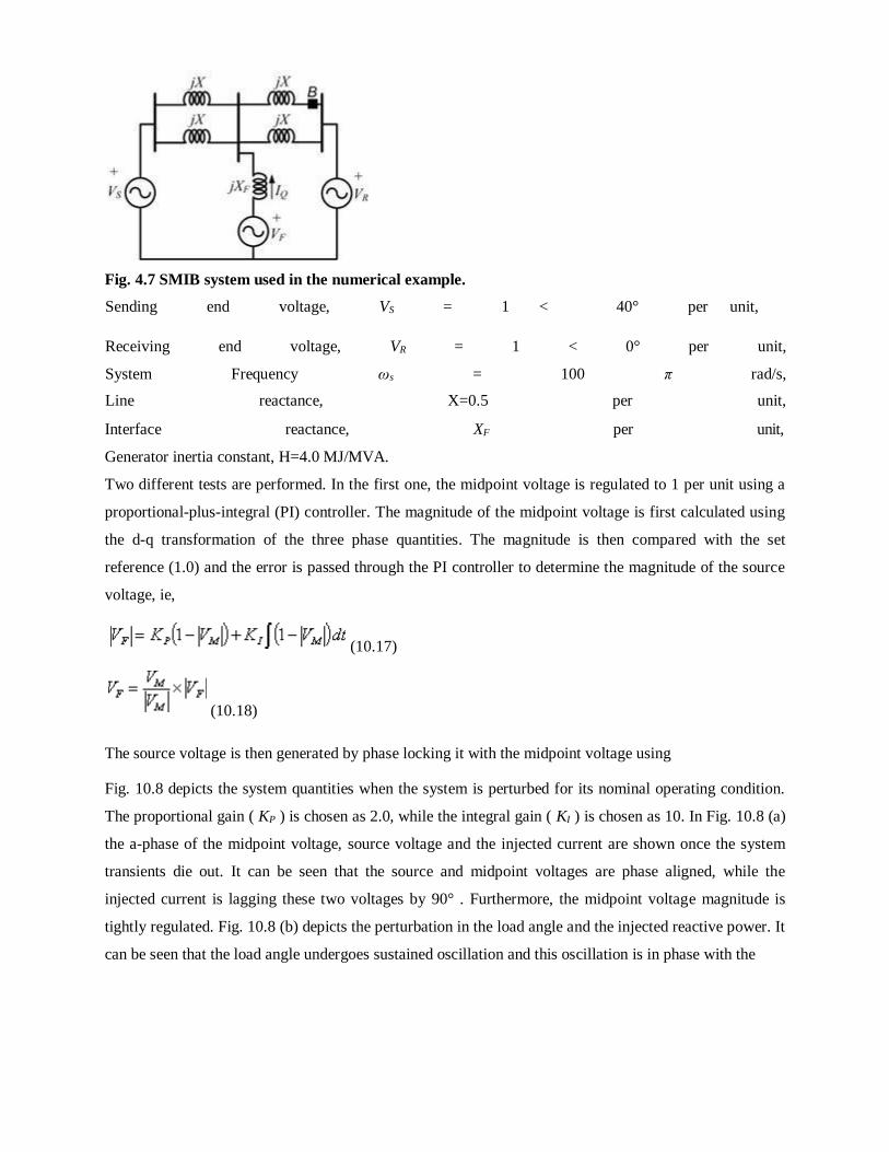
Fig. 4.7 SMIB system used in the numerical example.
Sending end voltage, VS = 1 < 40° per unit,
Receiving end voltage, VR = 1 < 0° per unit,
System Frequency ωs = 100 π rad/s,
Line reactance, X=0.5 per unit,
Interface reactance, XF per unit,
Generator inertia constant, H=4.0 MJ/MVA.
Two different tests are performed. In the first one, the midpoint voltage is regulated to 1 per unit using a
proportional-plus-integral (PI) controller. The magnitude of the midpoint voltage is first calculated using
the d-q transformation of the three phase quantities. The magnitude is then compared with the set
reference (1.0) and the error is passed through the PI controller to determine the magnitude of the source
voltage, ie,
(10.17)
(10.18)
The source voltage is then generated by phase locking it with the midpoint voltage using
Fig. 10.8 depicts the system quantities when the system is perturbed for its nominal operating condition.
The proportional gain ( KP ) is chosen as 2.0, while the integral gain ( KI ) is chosen as 10. In Fig. 10.8 (a)
the a-phase of the midpoint voltage, source voltage and the injected current are shown once the system
transients die out. It can be seen that the source and midpoint voltages are phase aligned, while the
injected current is lagging these two voltages by 90° . Furthermore, the midpoint voltage magnitude is
tightly regulated. Fig. 10.8 (b) depicts the perturbation in the load angle and the injected reactive power. It
can be seen that the load angle undergoes sustained oscillation and this oscillation is in phase with the
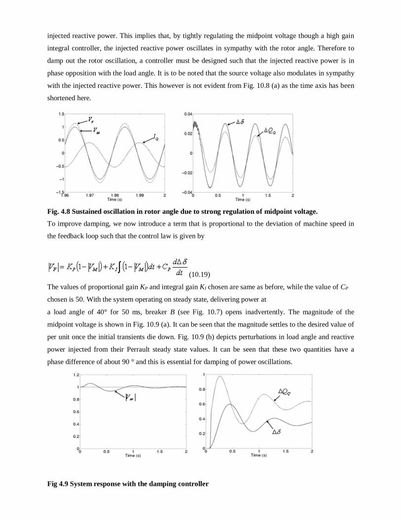
Smartzworld.com Smartworld.asia
jntuworldupdates.org Specworld.in
injected reactive power. This implies that, by tightly regulating the midpoint voltage though a high gain
integral controller, the injected reactive power oscillates in sympathy with the rotor angle. Therefore to
damp out the rotor oscillation, a controller must be designed such that the injected reactive power is in
phase opposition with the load angle. It is to be noted that the source voltage also modulates in sympathy
with the injected reactive power. This however is not evident from Fig. 10.8 (a) as the time axis has been
shortened here.
Fig. 4.8 Sustained oscillation in rotor angle due to strong regulation of midpoint voltage.
To improve damping, we now introduce a term that is proportional to the deviation of machine speed in
the feedback loop such that the control law is given by
(10.19)
The values of proportional gain KP and integral gain KI chosen are same as before, while the value of CP
chosen is 50. With the system operating on steady state, delivering power at
a load angle of 40° for 50 ms, breaker B (see Fig. 10.7) opens inadvertently. The magnitude of the
midpoint voltage is shown in Fig. 10.9 (a). It can be seen that the magnitude settles to the desired value of
per unit once the initial transients die down. Fig. 10.9 (b) depicts perturbations in load angle and reactive
power injected from their Perrault steady state values. It can be seen that these two quantities have a
phase difference of about 90 ° and this is essential for damping of power oscillations.
Fig 4.9 System response with the damping controller

Smartworld.asia
jntuworldupdates.org Specworld.in jntuworldupdates.org Specworld.in
Smartworld.asia
Section II: Ideal Series Compensator
Impact of Series Compensator on Voltage Profile
Improving Power-Angle Characteristics
An Alternate Method of Voltage Injection
Improving Stability Margin
Comparisons of the Two Modes of Operation
Power Flow Control and Power Swing Damping
Ideal Series Compensator
Let us assume that the series compensator is represented by an ideal voltage source. This is shown in Fig.
10.10. Let us further assume that the series compensator is ideal, i.e., it only supplies reactive power and
no real power to the system. It is needless to say that this assumption is not valid for practical systems.
However, for an introduction, the assumption is more than adequate. It is to be noted that, unlike the
shunt
Compensator, the location of the series compensator is not crucial, and it can be placed anywhere along
the transmission line.
Fig. 4.10 Schematic diagram of an ideal series compensated system.
Impact of Series Compensator on Voltage Profile
In the equivalent schematic diagram of a series compensated power system is shown in Fig. 10.10, the
receiving end current is equal to the sending end current, i.e., IS = IR . The series voltage VQ is injected in
such a way that the magnitude of the injected voltage is made proportional to that of the line current.
Furthermore, the phase of the voltage is forced to be in quadrature with the line current. We then have
(10.20)
The ratio λ/X is called the compensation level and is often expressed in percentage. This compensation
level is usually measured with respect to the transmission line reactance. For example, we shall refer the
compensation level as 50% when λ = X /2. In the analysis presented below, we assume that the injected
voltage lags the line current. The implication of the voltage leading the current will be discussed later.
Applying KVL we get

Smartzworld.com
jntuworldupdates.org Specworld.in
(10.21)
Assuming VS = V < δ and VR = V <0° , we get the following expression for the line current
When we choose VQ = λ IS e- j90° , the line current equation becomes
Thus we see that λ is subtracted from X . This choice of the sign corresponds to the voltage source acting
as a pure capacitor. Hence we call this as the capacitive mode of operation
In contrast, if we choose VQ = λIS e+j90° , λ is added to X , and this mode is referred to as the inductive
mode of operation . Since this voltage injection using (10.20) add λ to or subtract λ from the line
reactance, we shall refer it as voltage injection in constant reactance mode. We shall consider the
implication of series voltage injection on the transmission line voltage through the following example.
Example 4.3
Consider a lossless transmission line that has a 0.5 per unit line reactance (X). The sending end and
receiving end voltages are given by 1< δ and 1< 0° per unit respectively where δ is chosen as 30° .
Let us choose λ = 0.5 and operation in the capacitive mode. For this line, this implies a 30% level of line
impedance compensation. The line current is then given from (10.21) as IS = 1.479 7 < 15° per unit and
the injected voltage calculated from (10.20) is VQ = 0.2218 < - 75° per unit. The phasor diagrams of the
two end voltages, line current and injected voltage are shown in Fig. 10.11 (a). We shall now consider a
few different cases.
Let us assume that the series compensator is placed in the middle of the transmission line.
We then define two voltages, one at either side of the series compensator. These are:
Voltage on the left: VQL = VS - jXIS / 2 = 0.9723 < 8.45° per unit
Voltage on the right: VQR = VR + jXIS / 2 = 0.9723 < 21.55° per unit
The difference of these two voltages is the injected voltage. This is shown in Fig. 10.11 (b), where the
angle θ = 8.45° . The worst case voltage along the line will then be at the two points on either side of the
series compensator where the voltage phasors are aligned with the line current phasor. These two points
are equidistant from the series compensator. However, their particular locations will be dependent on the
system parameters.
As a second case, let us consider that the series compensator is placed at the end of the transmission line,
just before the infinite bus. We then have the following voltage
Voltage on the left of the compensator: VQL = VR + VQ = 1.0789 < - 11.46° per unit
This is shown in Fig. 10.11 (c). The maximum voltage rise in the line is then to the immediate left of the
compensator, i.e., at VQL . The maximum voltage drop however still occurs at the point where the voltage
jntuworldupdates.org Specworld.in
Smartzworld.com phasor is aligned with the line current phasor.
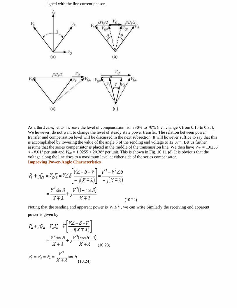
As a third case, let us increase the level of compensation from 30% to 70% (i.e., change λ from 0.15 to 0.35). We however, do not want to change the level of steady state power transfer. The relation between power
transfer and compensation level will be discussed in the next subsection. It will however suffice to say that this
is accomplished by lowering the value of the angle δ of the sending end voltage to 12.37° . Let us further
assume that the series compensator is placed in the middle of the transmission line. We then have VQL = 1.0255 < - 8.01° per unit and VQR = 1.0255 < 20.38° per unit. This is shown in Fig. 10.11 (d). It is obvious that the
voltage along the line rises to a maximum level at either side of the series compensator.
Improving Power-Angle Characteristics
(10.22)
Noting that the sending end apparent power is VS IS* , we can write Similarly the receiving end apparent
power is given by
(10.23)
(10.24)

Smartworld.asia
jntuworldupdates.org Specworld.in
Hence the real power transmitted over the line is given by
The power-angle characteristics of a series compensated power system are given in Fig. 10.12. In this
figure the base power is chosen as V2 / X . Three curves are shown, of which the curve P0 is the power-
angle curve when the line is not compensated. Curves which have maximum powers greater than the
base power pertain to capacitive mode of operation. On the other hand, all curves the inductive mode of
operation will have maximum values less than 1. For example, in Fig. 10.12, the curve P1 is for capacitive
mode and the curve P2 is for inductive mode of operation.
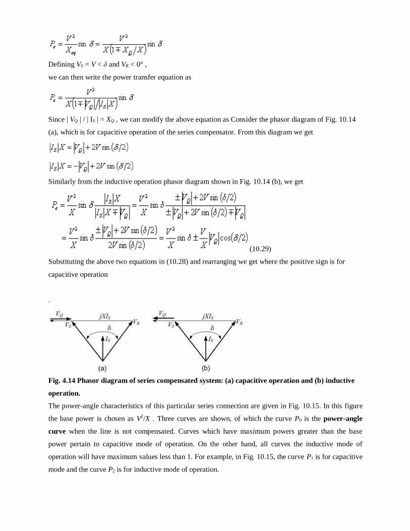
Fig. 4.12 Power-angle characteristics in constant reactance mode.
Let us now have a look at the reactive power. For simplicity let us restrict our attention to capacitive
mode of operation only as this represents the normal mode of operation in which the power transfer over
the line is enhanced. From (10.20) and (10.21) we get the reactive power supplied by the compensator as
Solving the above equation we get
(10.25)
In Fig. 10.13, the reactive power injected by the series compensator is plotted against the maximum
power transfer as the compensation level changes from 10% to 60%. As the compensation level increases,
the maximum power transfer also increases. However, at the same time, the reactive injection requirement
from the series compensator also increases. It is interesting to note that at 50% compensation level, the
reactive power injection requirement from a series compensator is same that from shunt compensator that
is regulating the midpoint voltage to 1.0 per unit.

jntuworldupdates.org Specworld.in
Smartzworld.com Smartworld.asia
Fig. 4.13 Reactive power injection by a series compensator versus maximum power transfer as the
level of compensation changes in constant reactance mode.
An Alternate Method of Voltage Injection
So far we have assumed that the series compensator injects a voltage that is in quadrature with the line
current and its magnitude is proportional to the magnitude of the line current. A set of very interesting
equations can be obtained if the last assumption about the magnitude is relaxed. The injected voltage is
then given by
(10.26)
We can then write the above equation as
(10.27)
the voltage source in quadrature with the current is represented as a pure reactance that is either inductive
or capacitive. Since in this form we injected a constant voltage in quadrature with the line current, we
shall refer this as constant voltage injection mode.
The total equivalent inductance of the line is then
Smartzworld.com Smartworld.asia
jntuworldupdates.org Specworld.in
Defining VS = V < δ and VR < 0° ,
we can then write the power transfer equation as
Since | VQ | / | IS | = XQ , we can modify the above equation as Consider the phasor diagram of Fig. 10.14
(a), which is for capacitive operation of the series compensator. From this diagram we get
Similarly from the inductive operation phasor diagram shown in Fig. 10.14 (b), we get
(10.29)
Substituting the above two equations in (10.28) and rearranging we get where the positive sign is for
capacitive operation
.
Fig. 4.14 Phasor diagram of series compensated system: (a) capacitive operation and (b) inductive
operation.
The power-angle characteristics of this particular series connection are given in Fig. 10.15. In this figure
the base power is chosen as V2/X . Three curves are shown, of which the curve P0 is the power-angle
curve when the line is not compensated. Curves which have maximum powers greater than the base
power pertain to capacitive mode of operation. On the other hand, all curves the inductive mode of
operation will have maximum values less than 1. For example, in Fig. 10.15, the curve P1 is for capacitive
mode and the curve P2 is for inductive mode of operation.

Smartzworld.com
Smartworld.asia
jntuworldupdates.org Specworld.in
Fig. 4.15 Power-angle characteristics for constant voltage mode
(10.30)
The reactive power supplied by the compensator in this case will be
Improving Stability Margin
From the power-angle curves of Figs. 10.13 and 10.15 it can be seen that the same amount of power can
be transmitted over a capacitive compensated line at a lower load angle than an uncompensated system.
Furthermore, an increase in the height in the power-angle curve means that a larger amount of
decelerating area is available for a compensated system. Thus improvement in stability margin for a
capacitive series compensated system over an uncompensated system is obvious.
Comparisons of the Two Modes of Operation
As a comparison between the two different modes of voltage injection, let us first consider the constant
reactance mode of voltage injection with a compensation level of 50%. Choosing V2 / X as the base
power, the power-angle characteristic reaches a maximum of 2.0 per unit at a load angle π / 2. Now | VQ |
in constant voltage mode is chosen such that the real power is 2.0 per unit at a load angle of π / 2. This is
accomplished using (10.29) where we get
Per unit
The power-angle characteristics of the two different modes are now drawn in Fig. 10.16 (a). It can be seen
that the two curves match at π / 2. However, the maximum power for constant voltage case is about 2.1
per unit and occurs at an angle of 67° .
Fig. 10.16 (b) depicts the line current for the two cases. It can be seen that the increase in line current in
either case is monotonic. This is not surprising for the case of constant reactance mode since as the load

Smartzworld.com
Smartworld.asia
jntuworldupdates.org Specworld.in
angle increases, both real power and line currents increase. Now consider the case of constant voltage
control. When the load angle moves backwards from π /2 to 67°, the power moves from 2.0 per unit to its
peak value of 2.1 per unit. The line current during this stage decreases from about 2.83 to 2.50 per unit.
Thus, even though the power through the line increases, the line current decreases.
Power Flow Control and Power Swing Damping
One of the major advantages of series compensation is that through its use real power flow over
transmission corridors can be effectively controlled. Consider, for example, the SMIB system shown in
Fig. 10.17 in which the generator and infinite bus are connected through a double circuit transmission
line, labeled line-1 and line-2. Of the two transmission lines, line-2 is compensated by a series
compensator. The compensator then can be utilized to regulate power flow over the entire system.
Fig. 4.16 Power-angle and line current-angle characteristics of the two different methods of voltage
injection: solid line showing constant reactance mode and dashed line showing constant voltage
mode.
For example, let us consider that the system is operating in the steady state delivering a power of Pm0 at a
load angle of δ0 . Lines 1 and 2 are then sending power Pe1 and Pe2 respectively, such that Pm0 = Pe1 + Pe2 .
The mechanical power input suddenly goes up to Pm1 . There are two ways of controlling the power in this
situation:
Regulating Control: Channeling the increase in power through line-1. In this case the series
compensator maintains the power flow over line-2 at Pe2 . The load angle in this case goes up in
sympathy with the increase in Pe1 .
Tracking Control: Channeling the increase in power through line-2. In this case the series
compensator helps in maintaining the power flow over line-1 at Pe1 while holding the load angle
to δ0 .
Let us illustrate these two aspects with the help of a numerical example.

Smartzworld.com Smartworld.asia
jntuworldupdates.org Specworld.in
Example 4.4
Let us consider the system of Fig. 7.8 where the system parameters are given by
System Frequency = 50 Hz, | V S | = | V R | = 1.0 per unit, X = 0.5 per unit and d 0 = 30 ° /
It is assumed that the series compensator operates in constant reactance mode with a compensation level
of 30%. We then have
Pe1 = 1.0 per unit, Pe2 = 1.43 per unit, Pm = 2.43 per unit
The objective of the control scheme here is to maintain the power through line-2 to a pre-specified value,
Pref . To accomplish this a proportional-plus-integral (PI) controller is placed in the feedback loop of Pe2 .
In addition, to improve damping a term that is proportional to the deviation of machine speed is
introduced in the feedback loop. The control law is then given by
(10.31)
Where CL = λ / X is the compensation level. For the simulation studies performed, the following controller
parameters are chosen
KP = 0.1, KI = 1.0 and CP = 75
Regulating Control: With the system operating in the nominal steady state, the mechanical power input
is suddenly raised by 10%. It is expected that the series compensator will hold the power through line-2
constant at line-2 at Pe2 such that entire power increase is channeled through line-1. We then expect that
the power Pe1 will increase to 1.243 per unit and the load angle to go up to 0.67 rad. The compensation
level will then change to 13%.
The time responses for various quantities for this test are given in Fig. 10.18. In Fig. 10.18 (a), the power
through the two line is plotted. It can be seen that while the power through line-2 comes back to its
nominal value following the transient, the power through the other line is raised to expected level.
Similarly, the load angle and the compensation level reach their expected values, as shown in Figs. 10.18
(b) and (c), respectively. Finally, Fig. 10.18 (d) depicts the last two cycles of phase-a of the line current
and injected voltage. It can be clearly seen that these two quantities are in quadrature, with the line current
leading the injected voltage.

Smartzworld.com Smartworld.asia
jntuworldupdates.org Specworld.in
Fig. 4.18 System response with regulating power flow controller Tracking Control
With the system operating in the nominal steady state, the mechanical power input is suddenly raised by
25%. It is expected that the series compensator will make the entire power increase to flow through line-2
such that both Pe1 and load angle are maintained constant at their nominal values. The power Pe2 through
line-2 will then increase to about 2.04 per unit and the compensation level will change to 51%.
The time responses for various quantities for this test are given in Fig. 10.19. It can be seen that while the
power through line-1 comes back to its nominal value following the transient, the power through the other
line is raised to level expected. Similarly, the load angle comes back to its nominal value and the
compensation level is raised 51%, as shown in Figs. 10.19 (b) and (c), respectively. Finally, Fig. 7.19 (d)
depicts the last two cycles of phase-a of the line current and injected voltage.
Fig. 4.19 System response with regulating power flow controller

UNIT- V
POWER SYSTEM OPERATION IN COMPETITIVE ENVIRONMENT
1.1. INTRODUCTION
Throughout the world, electric power utilities are currently undergoing major restructuring process
and are adopting the deregulated market operation. Competition has been introduced in power
systems around the world based on the promise that it will increase the efficiency of the industrial sector and reduce the cost of electrical energy of all customers. Electrical energy could not be
stored in large quantities. Continuity of supply is sought as more important than the cost of the
electrical energy. To meet the growing power demand, electric power industry has to adopt the deregulated structure.
For integrated operation of deregulated system, regulating agencies such as pool operator or
system operator have to be formulated. In the deregulated power market, the electricity is
dispatched with the help of either by a separate power exchange or the system 1 pool operator.
The power system deregulation is expected to offer the benefit of lower electricity price, better
consumer senice and improved system efficiency. However, it poses several technical challenges
with respect to its conceptualization and integrated operation. Basic issues of ensuring economical, secured and stable operation of the power system, which can deliver the power at desired quality,
has to be addressed carefully in a deregulated market. The complexity is more in such an
arrangement.
Power systems, all over the world, have been forced to operate to their full capacities due to the
environmental and I or economical constraints. This results in the need of new generation centers and bansmission lines. The amount of electric power that can be misaimed between two locations
through a tmsmission network is also limited by security constraints. Power flows should not be
allowed to increase to a level where a random event could cause the network to collapse due to
overloading, angular instability, voltages instability or cascaded outages. This state of the system is called as congestion of the power system. Managing congestion to minimize the restrictions of the
transmission network becomes the central activity of power system operators in recent The
deregulation of the electric utility industry allows many independent power producers (IPP) to be
connected across the transmission system. This situation also calls for effective methods to ensure
the transmission system reliability, while the power is msfemd through the network.
In a deregulated environment, there are many simultaneous bilateral and multilateral transactions
in addition to power pooling. Therefore, it is very much important that sellers and buyers of electricity need to fmd the cost allocation to their wheeling transactions. Independent System
Operator (ISO), a supreme entity for the control of transmission system, also needs to know such
costs in order to make correct economic and engineering decisions on up&ng the hmsmission facilities. So wheeling is currently a high priority problem in both regulated and deregulated power
industries. Transmission Open Access (TOA) is an important step for the translation of
conventional power systems to a deregulated power system. It consists of the regulatory structure, which includes transmission righf obligations, operational procedures and economic conditions of
the system and enables two or more parties to use the transmission network for electricity power
transfer of another party. This concept is gaining deep attention which desire to introduce
competition into traditional regulated utilities without giving up their existing regulatory structure. Such a deregulated system study is carried out in the present thesis work. Before entRing into the
details of the work, important terms used have bccn explained in the following section.
BASIC CONCEPTS
Wheeling
Wheeling is the transmission of power from a seller to a buya through a third party network. It may
be defined as," the use of transmission or distribution facilities of a system to transmit power of
and for another entity or entities" . It may also be defined as:' Wheeling is the use of some party's

(or parties') transmission system(s) for the benefit of the other parties".
Bilatera1 Wheeling Transaction It is a bilateral exchange of power between a buying and selling
entity. The exchange may be a proposed, scheduled or actual one.
Multilateral Wheeling Transactions
Multilateral transactions are an extension of bilateral transactions. In a multilateral transaction,
power is injected at different buses and taken out at some other different buses simultanmusly,
such that the sum of all generations is equal to all loads in the transaction, excluding losses. Transmission losses may be either supplied by the generators of the transactions or by the pool 1
utility as per predefined contract. This trade is arranged by energy brokers and involves more than
two parties.
Transmission Open Access (TOA)
Because of transmission open access, entities that did not own bansmission lines were granted the
right to use the transmission system. The aim of TOA is to introduce competition into the
traditional regulated utilities without giving up the existing regulating structure.
Resfructuring
Restmcturing of regulated power se~toris to separate the functions of power generation,
transmission, distribution and electricity supply to consumers.
Deregulation
It is changing the existing monopoly franchise rule or other regulations of regulated industry, that
affect how electric companies do business, and how customers may buy electric power and
services .
Awilable Transfer Capability (ATC)
The ATC is a measure of the transfer capability remaining in the physical transmission network for
further commercial activity over and above already committed uses.
Toul Tnrnsfer Capability (TTC)
It is defined as the amount of electric power that can be transferred over the interconnected
tnmmission network or particular path or interface in a reliable manner, while meeting all of a well
defined pre- and postcontingency system conditions from a specified set.
Transmission Relhbili@ Margin (TRM)
It is defined as that amount of transmission transfer capability necessary to ensure that the
interconnected transmission network is secured under a reasonable range of uncertainties in the
system.
Capaciry Bencft Mcvgr'n (CBM)
It is defrned as that amount of transmission transfer capability reserved for load serving entities on
the host transmission system to ensure access to generation from interconnected systems to meet
generation reliability requirements.
Short Run Marginal Cod (SRMC)
Short run marginal cost of wheeling transactions for a unit megawatt in deregulated environment is
calculated by taking into account the difference between bus incremental costs of the buses for producing an additional mega watt at each bus.
Embedded Cost
Embedded cost is defined as the revenue requirements needed to pay for all existing transmission
facilities plus any new facilities added to the transmission network during the life of the contract for transmission service.

Transmission System Congestion
In a competitive electricity market, congestion refers to the overloading of lines or traasfonnas due
to market settlement. The chances of congestion in the deregulated market are quite high as compared to the monopolistic market, as the customen would like to purchase electricity from the
cheapest available sources. The congestion is undesirable in the system and should be alleviated
for the secure operation of the system.
DEREGULATION IN POWER INDUSTRY
The driving force behiid the development of power systems is the growing demand for electrical
energy in developing countries. The energy demand will be the greatest in the near future. As
energy demand continues to grow, higher voltage levels are needed. In the beginning, A.C. transmission has to transfer power over long distances. In such transmission, technical problems
such as voltage control and dynamic stability will arise. This involves in heavy pricing over the
customer. The deregulated power system is to give opportunity to the customer to buy energy at a more favorable price.
The electric supply industry in every country for about the last one hundred years has been a
natural monopoly and as a monopoly attracted regulation by government. Without exception, the
industry has been operated as a vertically integrated monopoly organization that owned the
generation, transmission and distribution facilities. It was also a local monopoly, in the sense that
in any area one company or government agency sold electric power and services to all customers. The major difference between conventional monopolistic electricity market and the emerging
deregulated market is that electricity in the forma case is considered as merely energy supply
sector, whmas in the latter case it is treated as a service sector and is to be marketed like any other common commodity. In a monopolistic market, the same agency is respmible for power
generation, transportation, distribution as well as conkol, whereas in the new market structure these
tasks are segregated and have to be separately paid by the transacting parties. In the conventional market, the single utility is responsible for maintaining physical flow of electricity, satisfying
consumer's demands at proper voltage and6equmcy level, security, cconomy and reliability of the
system. In the newmated electricity market, of these tasks arc treated as separate services, in
addition to the primary task of the system operator and wire companies to ensure meetin the powa transactions all the time. The additid suvices include afianging powa for the loss makeup or load
following, maintaining the system kquacy, providing enough voltage I VAR support, arranging for
start-up power, spinning reserve in the system dc.
These arc called ancillary senices in the deregulated environment and have to bearrang ed and paid
sepsratcly. Some of these ancillary services can directly be arranged by the seller I buyas of electricity. In addition, the transmission of electricity itself will be treated as a separate mice and
has to be changed from the transacting parties and paid to the wire companies.
Motivations for Deregulated Power Industry
Since the 1980's the electricity supply indusby has been undergoing rapid andim nsible changes
wingth e indushy that is markably stable and served the public well. A significant feature of these
changes is that it allows for competition amo ng genwn and create marlra conditions in the
industry, which are seen as mccssary toreduce costs of energy production and diseibution, eliminate certain inefficiencies, shed manpower and increase customer choice. This transition
towards a deregulated powa mukt is commonly reid to as electricity supply industry restruchuing
or duegldation. South American countria such as Argentina and Chile, wac the first few to
introduce daqulrral marlrd of electricity in the mideighties followed by U.K., Sdviniw countries
and the USA in the 1990s, whac it is now fully operational. Some of the Asian countries, including India, have already taken initial steps in this direction.
In India, a limited level of competition is already introduced a! generation level by allowing
participation of Mepardeat Power Producers (IPPs). In addition, sepatation of threc organs of
power system i.e. gentration, bansmission and distribution has already been hein a few states.
Shortly most of the pwa utilities in the country will be adopting the daegulated structure in some
scnsc. Further, the ngulaiory bodies have been formed at central level and also at some of the
states. Their primary function, at present, is to fix tariff for power sales. Many factors such as
technology advances, changes in political and ideological attitudes, regulatory failures, high tariffs,
managerial inadequacy, global financial drives, the rise of environmentalism, and the shortage of public resources for investment in developing countries, contributed to the worldwide bud towards
deregulation.
Elements of Rabuetutcd Syrtcms
The structural components representing various segments of the deregulated electricity markd are
Generation companies (Gencos). Distribution companies (Discos), Scheduling Chudhon (SCs),
Transmission Ownas (TOs), an Independent System Operator (ISO). and a Power Exchange (PX).
Ccncos Garos art rsponsible for operating and maintaining generating plant in the generation sector and in most of the cays are the owners of the plant Where he transmission network was
state-owned before restructuring, obviously This integrity will be retained and a distinction
between owner and operator is redundant.
lndependent System Operator (ISO)
To achieve these objectives, the IS0 perfonus one or more of the following functions.
I. Power system operations function
This fundamental hraction includes the operation-planning fuoctim and realtime control.
a. Opaation-planning function includes
i. Perfonn power system scheduling.
ii. Coodnation with energy markets.
iii. Perform power system dispatch.
iv. Dctmnine Available Transfer Capabilities (ATCs).
v. Determine real-time ATCs.
vi. Pncalculate short-nm costs aod prices.
vii. Calculate hourly prices for transmission-related services.
b. Real-time control includes
i. Monitor power system operation status.
ii. Monitor sysdcm security.
iii. Conduct physical network operations and network switching.
iv. Deal with outages and emergencies.
v. Coordinalc real-time systan operation.
vi. Run a power pool where @a can bid to buy and sell magy.
vii. Submit the supply and load scbcdule to the IS0 according to pn-specified protocols.
11. Ancillary rcrvica provision function
i. Own certain ancillary services for satisfactory grid operation.
ii. Rvchase ancillary services transactions from market participants according to prc-specified
protocols.
iii. Provide ancillary services to transmission users.

iv. Allocate costs of ancillary services among all usm.
UI. Tnnsmiuioa facilities provision funetion
i. Maintain the transmission network.
ii. Provide transmission facilities for all supplies and loads.
iii. Plan transmission, reactive powcr and FAmS expansion.
iv. Plan and commissionowned ancillary snvices.
Related Documents