ELEC0047 - Power system dynamics, control and stability Transient stability analysis and improvement Thierry Van Cutsem [email protected] www.montefiore.ulg.ac.be/~vct November 2019 1 / 33

Welcome message from author
This document is posted to help you gain knowledge. Please leave a comment to let me know what you think about it! Share it to your friends and learn new things together.
Transcript

ELEC0047 - Power system dynamics, control and stability
Transient stability analysis and improvement
Thierry Van [email protected] www.montefiore.ulg.ac.be/~vct
November 2019
1 / 33
Transient stability analysis and improvement Introduction
(Rotor) angle stability
Most of the electrical energy is generated by synchronous machines
in normal system operation:
all synchronous machines rotate at the same electrical speed 2πfthe mechanical and electromagnetic torques acting on the rotating masses ofeach generator balance each otherthe phase angle differences between the internal e.m.f.’s of the variousmachines are constant = synchronism
following a disturbance, there is an imbalance between the two torques andthe rotor speed varies
rotor angle stability deals with the ability to keep/regain synchronism afterbeing subject to a disturbance
2 / 33
Transient stability analysis and improvement Introduction
Small-disturbance angle stability
Small-signal (or small-disturbance) angle stability deals with the ability of thesystem to keep synchronism after being subject to a “small disturbance”
“small disturbances” are those for which the system equations can belinearized (around an equilibrium point)
tools from linear system theory can be used, in particular eigenvalue andeigenvector analysis
3 / 33
Transient stability analysis and improvement Introduction
Transient (angle) stability
Transient (angle) stability deals with the ability of the system to keepsynchronism after being subject to a large disturbance
typical “large” disturbances:
short-circuit cleared by opening of circuit breakersmore complex sequences: backup protections, line autoreclosing, etc.
the nonlinear variation of the electromagnetic torque with the phase angle ofthe machine’s internal e.m.f. must be taken into account
→ numerical integration of the differential-algebraic equations is used to assessthe system response
unacceptable consequences of transient instability:
generators losing synchronism are tripped by protections (to avoid equipmentdamages)large angle swings create long-lasting voltage dips that disturb customers.
4 / 33
Transient stability analysis and improvement Introduction
Remarks
Small-disturbance angle stability:
depends on operating point and system parameters
does not depend on the disturbance (assumed infinitesimal and arbitrary)
is a necessary condition for operating a power system (small disturbances arealways present !)
Transient stability:
depends on operating point and system parameters
depends on the disturbance also
- the system may be stable wrt disturbance D1 but not disturbance D2- if so, the system is insecure wrt D2, but as long as D2 does not happen, it can
operate. . .
5 / 33
Transient stability analysis and improvement Introduction
Objectives of this lecture
We focus on a simple system: one machine and one infinite bus
allows a complete analytical treatmentand, hence, a good understanding of behaviouris a good introduction to more complex systems
central derivation: equal-area criterion
analogy with pendulum motion in Mechanicslarge-disturbance stability analyzed through energy considerationscertainly the most classical power system stability development(can be found even in the simplest textbooks on power system analysis!).
6 / 33
Transient stability analysis and improvement “Classical model” of synchronous machine
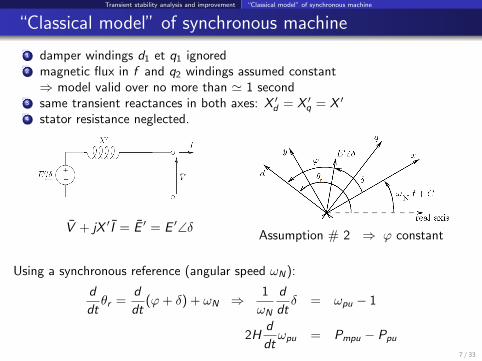
“Classical model” of synchronous machine
1 damper windings d1 et q1 ignored2 magnetic flux in f and q2 windings assumed constant⇒ model valid over no more than ' 1 second
3 same transient reactances in both axes: X ′d = X ′q = X ′
4 stator resistance neglected.
V + jX ′ I = E ′ = E ′∠δAssumption # 2 ⇒ ϕ constant
Using a synchronous reference (angular speed ωN):
d
dtθr =
d
dt(ϕ+ δ) + ωN ⇒ 1
ωN
d
dtδ = ωpu − 1
2Hd
dtωpu = Pmpu − Ppu
7 / 33
Transient stability analysis and improvement One-machine infinite-bus system under classical model
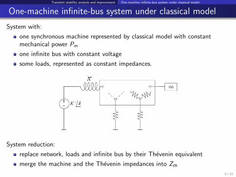
One-machine infinite-bus system under classical model
System with:
one synchronous machine represented by classical model with constantmechanical power Pm
one infinite bus with constant voltage
some loads, represented as constant impedances.
System reduction:
replace network, loads and infinite bus by their Thevenin equivalent
merge the machine and the Thevenin impedances into Zth
8 / 33
Transient stability analysis and improvement One-machine infinite-bus system under classical model
+
−+
−
Zth
Eth 6 θthE′ 6 δ
I
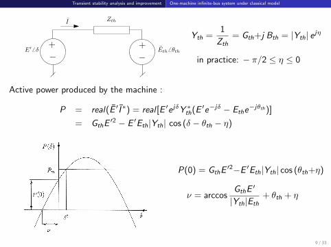
Yth =1
Zth= Gth+j Bth = |Yth| e jη
in practice: − π/2 ≤ η ≤ 0
Active power produced by the machine :
P = real(E ′ I ∗) = real [E ′e jδY ∗th(E ′e−jδ − Ethe−jθth)]
= GthE′2 − E ′Eth|Yth| cos (δ − θth − η)
P(0) = GthE′2−E ′Eth|Yth| cos (θth+η)
ν = arccosGthE
′
|Yth|Eth+ θth + η
9 / 33
Transient stability analysis and improvement Network configurations and equilibria
Network configurations and equilibria
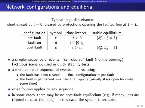
Typical large disturbance:short-circuit at t = 0, cleared by protections opening the faulted line at t = te
configuration symbol time interval stable equilibriumpre-fault v t < 0 (δov , ω
ov = 1)
fault-on d t ∈ [0 te ] -post-fault p t > te (δop , ω
op = 1)
a simpler sequence of events: “self-cleared” fault (no line opening).Fictitious scenario, used in quick stability tests
a more complex sequence of events: line reclosing
the fault has been cleared −→ final configuration = pre-faultthe fault is permanent −→ new line tripping (usually stays open for quitesome time)
what follows applies to any sequence
in some cases, there may be no post-fault equilibrium (e.g. if many lines aretripped to clear the fault). In this case, the system is unstable.
10 / 33
Transient stability analysis and improvement Network configurations and equilibria
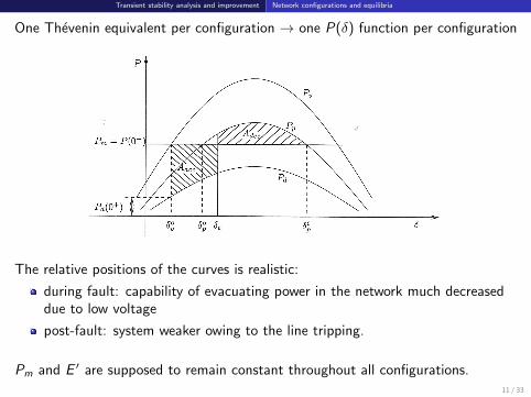
One Thevenin equivalent per configuration → one P(δ) function per configuration
The relative positions of the curves is realistic:
during fault: capability of evacuating power in the network much decreaseddue to low voltage
post-fault: system weaker owing to the line tripping.
Pm and E ′ are supposed to remain constant throughout all configurations.11 / 33
Transient stability analysis and improvement The equal-area criterion
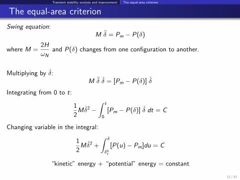
The equal-area criterion
Swing equation:M δ = Pm − P(δ)
where M =2H
ωNand P(δ) changes from one configuration to another.
Multiplying by δ:M δ δ = [Pm − P(δ)] δ
Integrating from 0 to t:
1
2M δ2 −
∫ t
0
[Pm − P(δ)] δ dt = C
Changing variable in the integral:
1
2M δ2 +
∫ δ
δ0v
[P(u)− Pm]du = C
“kinetic” energy + “potential” energy = constant
12 / 33
Transient stability analysis and improvement The equal-area criterion
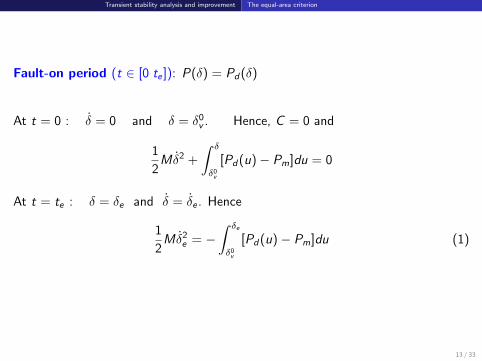
Fault-on period (t ∈ [0 te ]): P(δ) = Pd(δ)
At t = 0 : δ = 0 and δ = δ0v . Hence, C = 0 and
1
2M δ2 +
∫ δ
δ0v
[Pd(u)− Pm]du = 0
At t = te : δ = δe and δ = δe . Hence
1
2M δ2
e = −∫ δe
δ0v
[Pd(u)− Pm]du (1)
13 / 33
Transient stability analysis and improvement The equal-area criterion
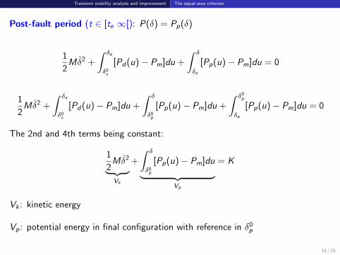
Post-fault period (t ∈ [te ∞[): P(δ) = Pp(δ)
1
2M δ2 +
∫ δe
δ0v
[Pd(u)− Pm]du +
∫ δ
δe
[Pp(u)− Pm]du = 0
1
2M δ2 +
∫ δe
δ0v
[Pd(u)− Pm]du +
∫ δ
δ0p
[Pp(u)− Pm]du +
∫ δ0p
δe
[Pp(u)− Pm]du = 0
The 2nd and 4th terms being constant:
1
2M δ2︸ ︷︷ ︸Vk
+
∫ δ
δ0p
[Pp(u)− Pm]du︸ ︷︷ ︸Vp
= K
Vk : kinetic energy
Vp: potential energy in final configuration with reference in δ0p
14 / 33
Transient stability analysis and improvement The equal-area criterion
15 / 33
Transient stability analysis and improvement The equal-area criterion
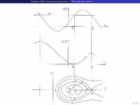
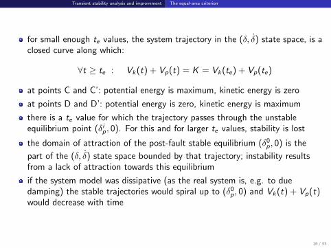
for small enough te values, the system trajectory in the (δ, δ) state space, is aclosed curve along which:
∀t ≥ te : Vk(t) + Vp(t) = K = Vk(te) + Vp(te)
at points C and C’: potential energy is maximum, kinetic energy is zero
at points D and D’: potential energy is zero, kinetic energy is maximum
there is a te value for which the trajectory passes through the unstableequilibrium point (δip, 0). For this and for larger te values, stability is lost
the domain of attraction of the post-fault stable equilibrium (δ0p, 0) is the
part of the (δ, δ) state space bounded by that trajectory; instability resultsfrom a lack of attraction towards this equilibrium
if the system model was dissipative (as the real system is, e.g. to duedamping) the stable trajectories would spiral up to (δ0
p, 0) and Vk(t) + Vp(t)would decrease with time
16 / 33
Transient stability analysis and improvement The equal-area criterion
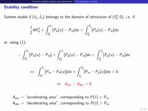
Stability condition
System stable if (δe , δe) belongs to the domain of attraction of (δ0p, 0), i.e. if
1
2M δ2
e +
∫ δe
δ0p
[Pp(u)− Pm]du <
∫ δip
δ0p
[Pp(u)− Pm]du
or, using (1):
−∫ δe
δ0v
[Pd(u)− Pm] +
∫ δe
δ0p
[Pp(u)− Pm]du <
∫ δip
δ0p
[Pp(u)− Pm]du
⇔∫ δe
δ0v
[Pm − Pd(u)]du +
∫ δip
δe
[Pm − Pp(u)]du < 0
⇔ Aacc − Adec < 0
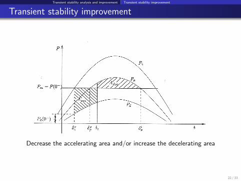
Aacc = “accelerating area”, corresponding to P(δ) < Pm
Adec = “decelerating area”, corresponding to P(δ) > Pm.
17 / 33
Transient stability analysis and improvement Critical clearing time
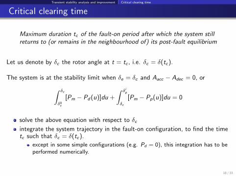
Critical clearing time
Maximum duration tc of the fault-on period after which the system stillreturns to (or remains in the neighbourhood of) its post-fault equilibrium
Let us denote by δc the rotor angle at t = tc , i.e. δc = δ(tc).
The system is at the stability limit when δe = δc and Aacc − Adec = 0, or∫ δc
δ0v
[Pm − Pd(u)]du +
∫ δip
δc
[Pm − Pp(u)]du = 0
solve the above equation with respect to δcintegrate the system trajectory in the fault-on configuration, to find the timetc such that δc = δ(tc).
except in some simple configurations (e.g. Pd = 0), this integration has to beperformed numerically.
18 / 33
Transient stability analysis and improvement Extensions of the equal-area criterion
Extensions of the equal-area criterion
Accounting for damping
stability becomes asymptotic
equal-area criterion pessimistic in terms of δc and tc
the first angle deviation is little decreased by damping. Damping is effectivein subsequent oscillations, for which a more detailed model is required.
19 / 33
Transient stability analysis and improvement Extensions of the equal-area criterion
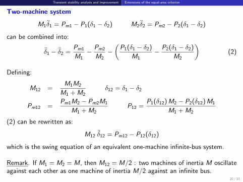
Two-machine system
M1δ1 = Pm1 − P1(δ1 − δ2) M2δ2 = Pm2 − P2(δ1 − δ2)
can be combined into:
δ1 − δ2 =Pm1
M1− Pm2
M2−(P1(δ1 − δ2)
M1− P2(δ1 − δ2)
M2
)(2)
Defining:
M12 =M1M2
M1 + M2δ12 = δ1 − δ2
Pm12 =Pm1M2 − Pm2M1
M1 + M2P12 =
P1(δ12)M2 − P2(δ12)M1
M1 + M2
(2) can be rewritten as:
M12 δ12 = Pm12 − P12(δ12)
which is the swing equation of an equivalent one-machine infinite-bus system.
Remark. If M1 = M2 = M, then M12 = M/2 : two machines of inertia M oscillateagainst each other as one machine of inertia M/2 against an infinite bus.
20 / 33
Transient stability analysis and improvement Extensions of the equal-area criterion
Extensions to multi-machine systems ?
rigorously speaking, the equal-area criterion does not apply to systems withmore than two machines
but the underlying energy concept inspired much research into “directmethods” for transient stability analysis
it also inspired “hybrid” methods:
detailed time simulation complemented with stability assessment inspired ofequal-area criterionrelying on a two-machine equivalent: one machine corresponds to themachine(s) loosing synchronism, the other machine to the rest of the system
the concept of critical clearing time tc applies, whatever the complexity ofthe model
“critical group”: the set of machines which loose synchronism with respect tothe remaining of the system, for a clearing time a little larger than tc .
21 / 33
Transient stability analysis and improvement Transient stability improvement
Transient stability improvement
Decrease the accelerating area and/or increase the decelerating area
22 / 33
Transient stability analysis and improvement Transient stability improvement
Modifying the pre-disturbance operating point:
reducing the active power generation
operating with higher excitation
Automatic emergency controls:
actions on network:
line auto-reclosingfast series capacitor reinsertionfast fault clearing - single pole breaker operation
actions in generators:
(turbine) fast valvinggeneration shedding
action on “load”: dynamic braking
Other means:
equip generators with fast excitation system
control voltage at intermediate points in a long corridor: throughsynchronous condensers or static var compensators.
23 / 33
Transient stability analysis and improvement Modifying the pre-disturbance operating point
Modifying the pre-disturbance operating point
Active power generation
Decreasing Pm:
decreases the accelerating area
increases the decelerating area
(side effect: pre- and post-fault equilibria also modified)
Reactive power generation
E ′(0+) = E ′(0−) =
√(V + X ′
Q
V)2 + (X ′
P
V)2
For given values of V and P, increasing the reactive power production Qincreases the emf E ′ which prevails in the post-fault period
this, in turn, somewhat increases the magnitude of the P(δ) curve
and, hence, the decelerating area and the stability margin.
24 / 33
Transient stability analysis and improvement Line auto-reclosing
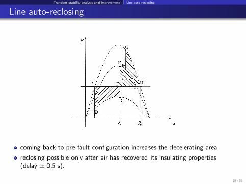
Line auto-reclosing
coming back to pre-fault configuration increases the decelerating area
reclosing possible only after air has recovered its insulating properties(delay ' 0.5 s).
25 / 33
Transient stability analysis and improvement Fault clearing
Fault clearing
Fault clearing delay:
should be as short as possible
typical values : 5 cycles (0.1 s at 50 Hz)
stability must be checked with respect to scenarios where primary protectionfails clearing the fault (due to protection or breaker malfunction), which iseliminated by the slower backup protection.
Single-phase tripping-reclosing:
most of the faults (' 75 %) are of the phase-ground type
for such faults, it is of interest to open the faulted phase only and keep theother two in service ⇒ protect each phase separately
in case of 3-phase fault with malfunction of one breaker, the other twooperate and the fault changes into phase-ground (less severe, cleared bybackup protection)
at EHV level, the three poles of the breaker are usually separate (for insulationreasons); it does not cost much to add a separate control on each phase.
26 / 33
Transient stability analysis and improvement Turbine fast valving
Turbine fast valving
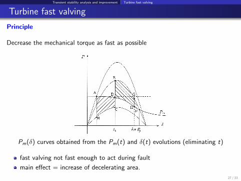
Principle
Decrease the mechanical torque as fast as possible
Pm(δ) curves obtained from the Pm(t) and δ(t) evolutions (eliminating t)
fast valving not fast enough to act during fault
main effect = increase of decelerating area.
27 / 33
Transient stability analysis and improvement Turbine fast valving
Speed of action
mechanical torque must be decreased rapidly: typically less than 0.5 s
gates of hydro turbines cannot be moved so quickly ⇒ applies to steamturbines
delays:
to take the decision from measurements (selectivity !)to close the valves. They are closed much faster than in normal operatingconditions by emptying the servomotor of its oil.
Decision criterion
cannot rely on rotor speed only: due to inertia it takes time to reach anemergency value
additional signal: rotor acceleration, drop of electrical power, differencebetween electrical power and an image of mechanical power.
28 / 33
Transient stability analysis and improvement Turbine fast valving
Implementation
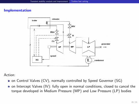
Action:
on Control Valves (CV), normally controlled by Speed Governor (SG)
on Intercept Valves (IV): fully open in normal conditions, closed to cancel thetorque developed in Medium Pressure (MP) and Low Pressure (LP) bodies
29 / 33
Transient stability analysis and improvement Turbine fast valving
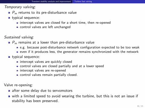
Temporary valving:
Pm returns to its pre-disturbance value
typical sequence:intercept valves are closed for a short time, then re-openedcontrol valves are left unchanged
Sustained valving:
Pm remains at a lower than pre-disturbance valuee.g. because post-disturbance network configuration expected to be too weakeven if it produces less, the generator remains synchronized with the network
typical sequence:intercept valves are quickly closedcontrol valves are closed partially and at a lower speedintercept valves are re-openedcontrol valves remain partially closed.
Valve re-opening:
after some delay due to servomotors
with a limited speed to avoid wearing the turbine, but this is not an issue ifstability has been preserved.
30 / 33
Transient stability analysis and improvement Generation shedding
Generation shedding
Principle
Trip one or several generators in order to preserve synchronous operation of theremaining generators
applies mainly to hydro plants
those including multiple generatorscombinations of 1, 2, 3, . . . generators can be dropped
may be also used with thermal plants:
tripped generator not stopped, used to feed its own auxiliaries(called tripping to houseload)plant remains in operation and can be re-synchronized with shorter delay
usually applies to large power plants evacuating power through long corridors.
31 / 33
Transient stability analysis and improvement Generation shedding
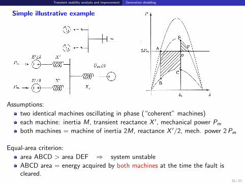
Simple illustrative example
Assumptions:
two identical machines oscillating in phase (“coherent” machines)
each machine: inertia M, transient reactance X ′, mechanical power Pm
both machines = machine of inertia 2M, reactance X ′/2, mech. power 2Pm
Equal-area criterion:
area ABCD > area DEF ⇒ system unstable
ABCD area = energy acquired by both machines at the time the fault iscleared.
32 / 33
Transient stability analysis and improvement Generation shedding
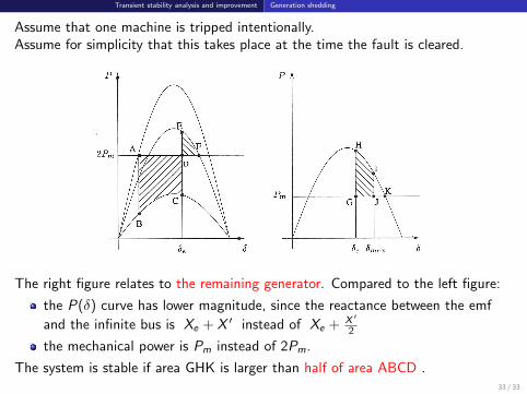
Assume that one machine is tripped intentionally.Assume for simplicity that this takes place at the time the fault is cleared.
The right figure relates to the remaining generator. Compared to the left figure:
the P(δ) curve has lower magnitude, since the reactance between the emf
and the infinite bus is Xe + X ′ instead of Xe + X ′
2
the mechanical power is Pm instead of 2Pm.
The system is stable if area GHK is larger than half of area ABCD .33 / 33
Related Documents