IEEE TRANSACTIONS ON COMPUTER-AIDED DESIGN OF INTEGRATED CIRCUITS AND SYSTEMS, VOL. 37, NO. 7, JULY 2018 1317 Power Grid Electromigration Checking Using Physics-Based Models Sandeep Chatterjee, Student Member, IEEE, Valeriy Sukharev, and Farid N. Najm, Fellow, IEEE Abstract—Due to technology scaling, electromigration (EM) signoff has become increasingly difficult, mainly due to the use of inaccurate methods for EM assessment, such as the empirical Black’s model. In this paper, we present a novel finite-difference- based approach for power grid EM checking using physics-based models, that can account for process, voltage, and temperature variations across the die. Our main contribution is to extend existing physical models for EM in metal branches to track EM degradation in multibranch interconnect trees. The extended model is represented as a homogeneous linear time invariant system. We also detect early failures and account for their impact on grid lifetime. We speed up our implementation by proposing a macromodeling-based filtering scheme and a predictor-based approach. Our results, for a number of IBM power grid bench- marks, confirm that Black’s model is overly inaccurate. The lifetimes found using our physics-based approach are on average 2.75× longer than those based on a (calibrated) Black’s model, as extended to handle mesh power grids. With a maximum runtime of 2.3 h among all the IBM benchmarks, our method appears to be suitable for very large scale integration circuits. Index Terms—Electromigration (EM), hydrostatic stress, linear time invariant (LTI) systems, macromodeling, power grid, reliability, verification. I. I NTRODUCTION A S A RESULT of continued scaling of integrated cir- cuits technology, electromigration (EM) has become a major reliability concern for the design of on-die power grids in large integrated circuits [1]. While signal and clock lines also suffer from EM degradation, these lines carry bidirec- tional current and so have longer lifetimes due to so-called healing. In contrast, power grid lines carry mostly unidi- rectional current with no benefit of healing and thus are more susceptible to EM failure. Hence, our focus on EM in power grids. Today, it is becoming harder to sign off on chip designs using state of the art EM checking tools, as there is very little margin left between the predicted EM stress and that allowed Manuscript received September 14, 2016; revised December 20, 2016; accepted January 26, 2017. Date of publication February 9, 2017; date of current version June 18, 2018. This work was supported in part by the Natural Sciences and Engineering Research Council of Canada, and in part by Mentor Graphics Corporation. This paper was recommended by Associate Editor Y. Cao. S. Chatterjee and F. N. Najm are with the Electrical and Computer Engineering Department, University of Toronto, Toronto, ON M5S 3G4, Canada (e-mail: [email protected]; [email protected]). V. Sukharev is with Mentor Graphics Corporation, Freemont, CA 94538 USA (e-mail: [email protected]). Color versions of one or more of the figures in this paper are available online at http://ieeexplore.ieee.org. Digital Object Identifier 10.1109/TCAD.2017.2666723 by EM design rules [2]. This loss of safety margin can be traced back to the inaccurate and oversimplified nature of EM models used by existing tools. Standard practice in the indus- try is to break up a grid into isolated metal branches, assess the reliability of each branch separately using Black’s model [3] and then use the series model (earliest branch failure time) to determine the failure time for the whole grid. This approach is highly inaccurate, for at least three reasons. First, the fitting parameters obtained for Black’s model under accelerated test- ing conditions are not valid at actual operating conditions, and this leads to significant errors in lifetime extrapolation [4], [5]. Second, Black’s model ignores the material flow between branches. In today’s mesh structured power grids, many branches within the same layer are connected as part of what is called an interconnect tree (defined later) and atomic flux can flow freely between the branches of an interconnect tree. As a result, if the individual branches happen to be short so that they are deemed immortal due to the Blech effect [6], then the tree would appear to be immortal, which is highly optimistic and can be entirely misleading for design. In fact, due to material flow across the tree, failures can and do happen even if the branches are short. On the other hand, because the assumption of no material flow between branches effectively means that the reliability of nearby metal lines are indepen- dent of each other, then the traditional approach can also be highly pessimistic, as we will see in this paper. Indeed, two identical connected lines that carry the same current density can in practice have quite different values of mean time to fail- ures (MTFs) [7], so that connected lines can influence each other leading to different mean lifetimes. Finally, the third problem lies with the series model assump- tion. A series model is the case where a power grid is deemed to have failed as soon as the first of its branches has failed, typically due to an open circuit. However, modern power grids use a mesh structure. As such, there are many paths for the current to flow from the C4 bumps to the underlying logic, a characteristic we refer to as redundancy. Mesh power grids are in fact closer to (but not quite) a parallel system. As such, it is highly pessimistic to assume that a single branch failure will always cause the whole grid to fail. Thus, there is a need to reconsider the traditional approaches and develop efficient EM checking techniques that can accu- rately assess EM degradation in large power grids. Over the last few years, many approaches have been proposed which overcome, to some extent, the aforementioned shortcomings. Chatterjee et al. [8] proposed the mesh model as an alternative to the series model. In the mesh model, a grid is deemed to have failed, not when the first line fails, 0278-0070 c 2017 IEEE. Personal use is permitted, but republication/redistribution requires IEEE permission. See http://www.ieee.org/publications_standards/publications/rights/index.html for more information.

Welcome message from author
This document is posted to help you gain knowledge. Please leave a comment to let me know what you think about it! Share it to your friends and learn new things together.
Transcript
IEEE TRANSACTIONS ON COMPUTER-AIDED DESIGN OF INTEGRATED CIRCUITS AND SYSTEMS, VOL. 37, NO. 7, JULY 2018 1317
Power Grid Electromigration CheckingUsing Physics-Based Models
Sandeep Chatterjee, Student Member, IEEE, Valeriy Sukharev, and Farid N. Najm, Fellow, IEEE
Abstract—Due to technology scaling, electromigration (EM)signoff has become increasingly difficult, mainly due to the useof inaccurate methods for EM assessment, such as the empiricalBlack’s model. In this paper, we present a novel finite-difference-based approach for power grid EM checking using physics-basedmodels, that can account for process, voltage, and temperaturevariations across the die. Our main contribution is to extendexisting physical models for EM in metal branches to trackEM degradation in multibranch interconnect trees. The extendedmodel is represented as a homogeneous linear time invariantsystem. We also detect early failures and account for their impacton grid lifetime. We speed up our implementation by proposinga macromodeling-based filtering scheme and a predictor-basedapproach. Our results, for a number of IBM power grid bench-marks, confirm that Black’s model is overly inaccurate. Thelifetimes found using our physics-based approach are on average2.75× longer than those based on a (calibrated) Black’s model, asextended to handle mesh power grids. With a maximum runtimeof 2.3 h among all the IBM benchmarks, our method appears tobe suitable for very large scale integration circuits.
Index Terms—Electromigration (EM), hydrostatic stress, lineartime invariant (LTI) systems, macromodeling, power grid,reliability, verification.
I. INTRODUCTION
AS A RESULT of continued scaling of integrated cir-cuits technology, electromigration (EM) has become a
major reliability concern for the design of on-die power gridsin large integrated circuits [1]. While signal and clock linesalso suffer from EM degradation, these lines carry bidirec-tional current and so have longer lifetimes due to so-calledhealing. In contrast, power grid lines carry mostly unidi-rectional current with no benefit of healing and thus aremore susceptible to EM failure. Hence, our focus on EM inpower grids.
Today, it is becoming harder to sign off on chip designsusing state of the art EM checking tools, as there is very littlemargin left between the predicted EM stress and that allowed
Manuscript received September 14, 2016; revised December 20, 2016;accepted January 26, 2017. Date of publication February 9, 2017; date ofcurrent version June 18, 2018. This work was supported in part by theNatural Sciences and Engineering Research Council of Canada, and in partby Mentor Graphics Corporation. This paper was recommended by AssociateEditor Y. Cao.
S. Chatterjee and F. N. Najm are with the Electrical and ComputerEngineering Department, University of Toronto, Toronto, ON M5S 3G4,Canada (e-mail: [email protected]; [email protected]).
V. Sukharev is with Mentor Graphics Corporation, Freemont, CA 94538USA (e-mail: [email protected]).
Color versions of one or more of the figures in this paper are availableonline at http://ieeexplore.ieee.org.
Digital Object Identifier 10.1109/TCAD.2017.2666723
by EM design rules [2]. This loss of safety margin can betraced back to the inaccurate and oversimplified nature of EMmodels used by existing tools. Standard practice in the indus-try is to break up a grid into isolated metal branches, assess thereliability of each branch separately using Black’s model [3]and then use the series model (earliest branch failure time) todetermine the failure time for the whole grid. This approachis highly inaccurate, for at least three reasons. First, the fittingparameters obtained for Black’s model under accelerated test-ing conditions are not valid at actual operating conditions, andthis leads to significant errors in lifetime extrapolation [4], [5].
Second, Black’s model ignores the material flow betweenbranches. In today’s mesh structured power grids, manybranches within the same layer are connected as part of whatis called an interconnect tree (defined later) and atomic fluxcan flow freely between the branches of an interconnect tree.As a result, if the individual branches happen to be short sothat they are deemed immortal due to the Blech effect [6],then the tree would appear to be immortal, which is highlyoptimistic and can be entirely misleading for design. In fact,due to material flow across the tree, failures can and do happeneven if the branches are short. On the other hand, because theassumption of no material flow between branches effectivelymeans that the reliability of nearby metal lines are indepen-dent of each other, then the traditional approach can also behighly pessimistic, as we will see in this paper. Indeed, twoidentical connected lines that carry the same current densitycan in practice have quite different values of mean time to fail-ures (MTFs) [7], so that connected lines can influence eachother leading to different mean lifetimes.
Finally, the third problem lies with the series model assump-tion. A series model is the case where a power grid is deemedto have failed as soon as the first of its branches has failed,typically due to an open circuit. However, modern power gridsuse a mesh structure. As such, there are many paths for thecurrent to flow from the C4 bumps to the underlying logic,a characteristic we refer to as redundancy. Mesh power gridsare in fact closer to (but not quite) a parallel system. As such,it is highly pessimistic to assume that a single branch failurewill always cause the whole grid to fail.
Thus, there is a need to reconsider the traditional approachesand develop efficient EM checking techniques that can accu-rately assess EM degradation in large power grids.
Over the last few years, many approaches have beenproposed which overcome, to some extent, the aforementionedshortcomings. Chatterjee et al. [8] proposed the mesh modelas an alternative to the series model. In the mesh model, agrid is deemed to have failed, not when the first line fails,
0278-0070 c© 2017 IEEE. Personal use is permitted, but republication/redistribution requires IEEE permission.See http://www.ieee.org/publications_standards/publications/rights/index.html for more information.
1318 IEEE TRANSACTIONS ON COMPUTER-AIDED DESIGN OF INTEGRATED CIRCUITS AND SYSTEMS, VOL. 37, NO. 7, JULY 2018
but when enough lines have failed so that the voltage drop atsome grid node(s) have exceeded some predefined threshold(which would cause errors in underlying logic). However, [8]still used Black’s model to compute the reliability of indi-vidual branches, which as we saw before is inaccurate.Huang et al. [9] proposed an adaptation of Korhonen’s phys-ical EM model [10] for interconnect trees. Hau-Riege andThompson [11] used Korhonen’s model to develop a closedform solution for stress evolution at a junction (a point wheremultiple branches meet) by replacing its connected brancheswith semi-infinite limbs, which was later used by Li et al. [12]in their EM verification tool. Both works [9], [12] were laterextended in [13], [14] respectively to account for tempera-ture variation as well. However, the approach in [9] is slow,requiring up to 32 h to estimate the failure time of a 400 knode grid. In [12], since the connected branches are replacedby semi-infinite limbs, atomic flow across the whole treeis not accounted for. Thus, there is a need for a new EMchecking approach that accurately models EM degradationusing physics-based models, combined with a mesh modelto account for redundancy, while being fast enough to bepractically useful.
In this paper, we propose such a technique, which is basedon a finite-difference-based physical EM checking approachthat accounts for process, voltage, and temperature variationsacross the die. A preliminary version of this paper is availablein [15]. We start with Korhonen’s 1-D physical model [10],and augment it: 1) by introducing boundary laws at junctionsto track the material flow and stress evolution in multibranchinterconnect trees (for arbitrary complex geometries) and2) by accounting for thermal stresses generated by nonuni-form temperature distribution across the grid. We refer tothis as the extended Korhonen’s Model. For each tree, theextended model starts out as a system of partial differentialequations (PDEs) coupled by boundary laws which we thendiscretize and scale to reduce it to a homogeneous linear timeinvariant (LTI) system, where each state represents the stressat a discretized point in the tree. We numerically solve thissystem to track the stress evolution over time and find thecorresponding time of void nucleations, some of which mightcause early failures (EFs) by disconnecting a via. As we willshow later, the impact of EF on grid reliability is quite severe,yet existing EM tools do not account for these failures.We are not aware of any published full-chip EM checkingapproach that can handle EFs. In this paper, we detectEFs and update the state of the system accordingly.We use the mesh model [8] to determinegrid failure.
The random nature of EM degradation, caused by processvariation, is taken care of by using a Monte Carlo method, inwhich successive samples of the grid time to failure (TTF) arefound, until the estimate of the overall MTF has converged.We improve our runtime by using a macromodeling-based fil-tering scheme that estimates up-front the active set of trees thatare most-likely to impact the MTF assessment of the grid, ascheme which we will show has minimal impact on accuracy.We also propose a predictive scheme that allows for fast MTFestimation based on extrapolation of the solution (stress curve)obtained from a few time-points. Testing this approach on the
IBM grid benchmarks [16], with the largest grid up to 720 knodes, shows that the MTF estimated using our physics-basedapproach are on average 2.75× longer than those based on a(calibrated) Black’s model. This justifies the claim that Black’smodel can be overly inaccurate for modern power grids andconfirms the need for physical models. With a run-time of2.3 h for the most difficult to solve grid and 26 min for thelargest (720 k) grid, this approach appears to be promising forlarge VLSI circuits.
The remainder of this paper is organized as follows. InSection II, we present some relevant background materialregarding EM, numerical methods for solving PDEs and statis-tical methods which we will use later in this paper. Section IIIdevelops the extended Korhonen’s model and Section IVdescribes the LTI system formulation used for numericallysolving the extended model. Section V summarizes theapproach we use to determine the temperature distribution andSection VI describes our overall power grid analysis approach.Section VII outlines the implementation details and discussesthe experimental results. Finally, Section VIII concludes thispaper.
II. BACKGROUND
A. Electromigration Basics
EM is the mass transport of metal atoms due to momentumtransfer between electrons (driven by an electric field) andthe atoms in a metal line. EM is highly dependent on thespecific microstructure of a given line. As such, due to randommanufacturing variations, the TTF due to EM is a randomvariable (RV). The process of EM degradation can be dividedinto two phases: 1) void nucleation and 2) void growth.
Under conditions of high current density, metal atoms arepushed in the direction of the electron flow, which is oppositeto the direction of the applied electric field. The number ofatoms moving across a cross section of a line per second perunit area is known as the atomic flux. If the in-flow of metalatoms is equal to the out-flow at every point on the line seg-ment, then clearly no deformation or failure will occur. On theother hand, if the in-flow is not equal to the out-flow, atomicflux divergence (AFD) is said to occur. AFD is a necessaryprerequisite for EM degradation and is typically observed inlocations with some kind of barrier to atomic movement, suchas at the end of a line, or due to a change in widths of con-nected branches or due to change in diffusivity around grainboundaries. Flux divergence at these locations generates pointsof high tensile and compressive stresses within the segment.The amount of compressive stress needed to cause a pile-upof metal atoms (a hillock) leading to a short circuit is veryhigh in modern metal systems, hence failure due to a shortcircuit is not usually observed. However, the build up of ten-sile stress eventually leads to formation of a void when thestress reaches a predetermined critical threshold. This phaseof EM degradation, when stress is increasing over time but novoids have yet nucleated, is called the void nucleation phase.In this phase, the resistance of a line remains roughly the sameas that of a fresh (undamaged) line.
Once a void nucleates, the void growth phase begins. Insome cases, depending on the geometry and the location of
CHATTERJEE et al.: POWER GRID EM CHECKING USING PHYSICS-BASED MODELS 1319
the void, nucleation by itself may be enough to cause failuredue to an open circuit (by disconnecting a via) [17]. Thesefailures are typically referred to as EFs and are often observedin testing. In other cases, again depending on geometry, a linemay continue to conduct current after void nucleation. Withtime, the void starts to grow in the direction of the electronflow and the line resistance increases toward some steady-statevalue. In testing of single isolated lines, failure is deemed tohappen when the increase in resistance reaches 10%–20% ofthe initial resistance value.
B. Korhonen Model
Korhonen et al. [10] proposed a 1-D model to describe thehydrostatic stress σ arising under the influence of EM. Here,hydrostatic stress is the average of all normal components ofthe full stress tensor, i.e., σ = (σxx + σyy + σzz)/3. Considera uniform metal line embedded in a rigid dielectric. We areinterested in the time-varying stress σ(x, t) at location x fromsome reference point, and at time t. Korhonen’s model startswith the following statement
�C(x, t)/
C(x, t) = −�σ(x, t)/
B (1)
where B is the bulk modulus and C is the number of metalatoms per unit volume, called the concentration of atoms. In anideal lattice with zero stress, C = 1/�, where � is the atomicvolume. Following Korhonen’s formulation, σ is positive fortensile stress and negative for compressive stress, and can beobtained by solving the PDE
∂σ
∂t= B�
kbTm
∂
∂x
{Da
(∂σ
∂x− q∗ρ
�j
)}(2)
where j is the current density in the line, Da is the coefficientof atomic diffusion, kb is the Boltzmann’s constant, Tm is thetemperature in Kelvin, q∗ is the absolute value of the effectivecharge of the conductor, and ρ is the resistivity of the con-ductor. The corresponding atomic flux Ja in the line can bewritten as [10], [18]
Ja = DaC�
kbTm
(∂σ
∂x− q∗ρ
�j
). (3)
Note that Ja can be positive or negative, depending on the ref-erence direction chosen and the actual direction of the electriccurrent. A void nucleates in the line once the stress exceeds apredefined threshold value σth > 0.
C. Diffusivity of Metal Lines
The atomic diffusion coefficient Da is usually expressedusing the Arrhenius law
Da = D0e−Q/(kbTm) (4)
where D0 is a constant and Q is the activation energy forvacancy formation and diffusion. The randomness in TTFdue to EM is primarily accounted for by the correspond-ing randomness in Da, which is lognormally distributed [19]with mean Davg. Strictly speaking, Da also depends on thestress value at a given point. However, it has been reportedthat the numerical results with stress dependent Da are “nottoo different” from constant Da [10]. Hence, as in many
Fig. 1. Cross sectional schematic of Cu dual damascene interconnects.
previous works [9], [12]–[14], we will assume that Da isstress-independent.
D. Method of Lines
The method of lines (MoLs) is a special finite-differencetechnique for solving PDEs [20]. The basic idea of MoL is todiscretize the PDE in all but one independent variable, so thatwe are left with a set of ordinary differential equations (ODEs)that approximate the PDE. We can then use well-establishedmethods to numerically solve the ODE.
Discretizing the PDE along any variable requires us toapproximate the partial derivatives. For a smooth functionf (xi, x2, . . . , xn), the partial derivative with respect to xi canbe approximated using a central difference formula [20]
∂f
∂xi(x) ≈ f (x + ei�x) − f (x − ei�x)
2�x(5)
∂2f
∂x2i
(x) ≈ f (x + ei�x) + f (x − ei�x) − 2f (x)
(�x)2(6)
where �x is a small positive scalar increment and ei is the ithunit vector (a vector that has 1 in position i and 0 elsewhere).
E. Limited Distributions
Let Y be an RV with cumulative distribution function (cdf)FY(t) and let l and u be two scalars with l < u and at least oneof them finite. Then, RV Y′ is called a limited RV betweenlimits l and u, with Y being the underlying RV, if it has thefollowing cdf [21]
FY ′(t) =⎧⎨
⎩
0, t < lFY(t), l ≤ t < u1, t ≥ u.
(7)
III. INTERCONNECT TREE EM ANALYSIS
Modern power grids are made of copper (Cu) and are fabri-cated using a dual damascene process. In a dual-damasceneprocess, the metal line and via are formed simultaneouslyusing copper. A barrier metal liner (usually Tantalum) mustcompletely surround all Cu interconnects to prevent the cop-per from diffusing into the surrounding dielectric. The crosssection of a typical metal via structure in a Cu dual dam-ascene process is as shown in Fig. 1. Every metal layer ofthe on-die power grid mostly consists of parallel stripes thatare connected by vias to other metal layers. Note that due tothe presence of the barrier metal liner around vias, Cu atomsfrom one layer cannot diffuse to another layer. On every layer,power and ground stripes are interspersed. As a result, the
1320 IEEE TRANSACTIONS ON COMPUTER-AIDED DESIGN OF INTEGRATED CIRCUITS AND SYSTEMS, VOL. 37, NO. 7, JULY 2018
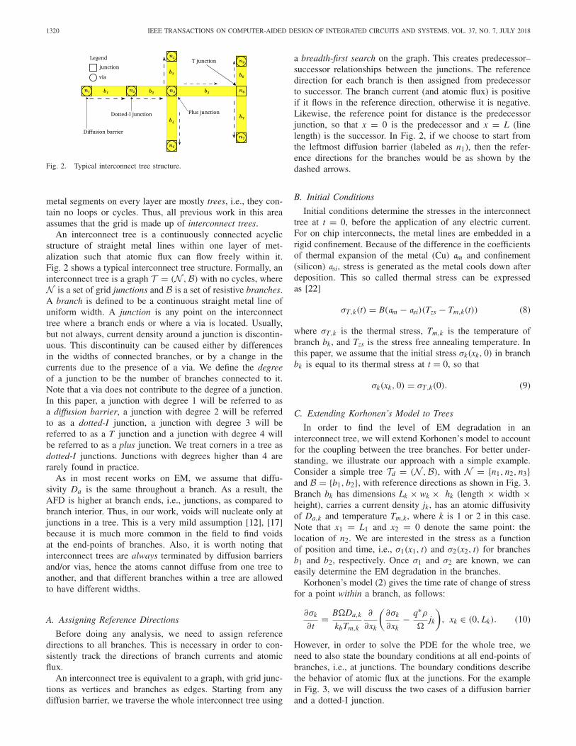
Fig. 2. Typical interconnect tree structure.
metal segments on every layer are mostly trees, i.e., they con-tain no loops or cycles. Thus, all previous work in this areaassumes that the grid is made up of interconnect trees.
An interconnect tree is a continuously connected acyclicstructure of straight metal lines within one layer of met-alization such that atomic flux can flow freely within it.Fig. 2 shows a typical interconnect tree structure. Formally, aninterconnect tree is a graph T = (N ,B) with no cycles, whereN is a set of grid junctions and B is a set of resistive branches.A branch is defined to be a continuous straight metal line ofuniform width. A junction is any point on the interconnecttree where a branch ends or where a via is located. Usually,but not always, current density around a junction is discontin-uous. This discontinuity can be caused either by differencesin the widths of connected branches, or by a change in thecurrents due to the presence of a via. We define the degreeof a junction to be the number of branches connected to it.Note that a via does not contribute to the degree of a junction.In this paper, a junction with degree 1 will be referred to asa diffusion barrier, a junction with degree 2 will be referredto as a dotted-I junction, a junction with degree 3 will bereferred to as a T junction and a junction with degree 4 willbe referred to as a plus junction. We treat corners in a tree asdotted-I junctions. Junctions with degrees higher than 4 arerarely found in practice.
As in most recent works on EM, we assume that diffu-sivity Da is the same throughout a branch. As a result, theAFD is higher at branch ends, i.e., junctions, as compared tobranch interior. Thus, in our work, voids will nucleate only atjunctions in a tree. This is a very mild assumption [12], [17]because it is much more common in the field to find voidsat the end-points of branches. Also, it is worth noting thatinterconnect trees are always terminated by diffusion barriersand/or vias, hence the atoms cannot diffuse from one tree toanother, and that different branches within a tree are allowedto have different widths.
A. Assigning Reference Directions
Before doing any analysis, we need to assign referencedirections to all branches. This is necessary in order to con-sistently track the directions of branch currents and atomicflux.
An interconnect tree is equivalent to a graph, with grid junc-tions as vertices and branches as edges. Starting from anydiffusion barrier, we traverse the whole interconnect tree using
a breadth-first search on the graph. This creates predecessor–successor relationships between the junctions. The referencedirection for each branch is then assigned from predecessorto successor. The branch current (and atomic flux) is positiveif it flows in the reference direction, otherwise it is negative.Likewise, the reference point for distance is the predecessorjunction, so that x = 0 is the predecessor and x = L (linelength) is the successor. In Fig. 2, if we choose to start fromthe leftmost diffusion barrier (labeled as n1), then the refer-ence directions for the branches would be as shown by thedashed arrows.
B. Initial Conditions
Initial conditions determine the stresses in the interconnecttree at t = 0, before the application of any electric current.For on chip interconnects, the metal lines are embedded in arigid confinement. Because of the difference in the coefficientsof thermal expansion of the metal (Cu) am and confinement(silicon) asi, stress is generated as the metal cools down afterdeposition. This so called thermal stress can be expressedas [22]
σT,k(t) = B(am − asi)(Tzs − Tm,k(t)) (8)
where σT,k is the thermal stress, Tm,k is the temperature ofbranch bk, and Tzs is the stress free annealing temperature. Inthis paper, we assume that the initial stress σk(xk, 0) in branchbk is equal to its thermal stress at t = 0, so that
σk(xk, 0) = σT,k(0). (9)
C. Extending Korhonen’s Model to Trees
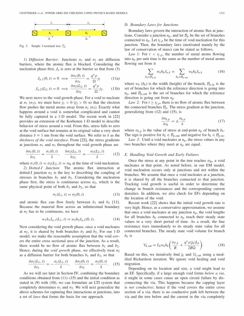
In order to find the level of EM degradation in aninterconnect tree, we will extend Korhonen’s model to accountfor the coupling between the tree branches. For better under-standing, we illustrate our approach with a simple example.Consider a simple tree Td = (N ,B), with N = {n1, n2, n3}and B = {b1, b2}, with reference directions as shown in Fig. 3.Branch bk has dimensions Lk × wk × hk (length × width ×height), carries a current density jk, has an atomic diffusivityof Da,k and temperature Tm,k, where k is 1 or 2 in this case.Note that x1 = L1 and x2 = 0 denote the same point: thelocation of n2. We are interested in the stress as a functionof position and time, i.e., σ1(x1, t) and σ2(x2, t) for branchesb1 and b2, respectively. Once σ1 and σ2 are known, we caneasily determine the EM degradation in the branches.
Korhonen’s model (2) gives the time rate of change of stressfor a point within a branch, as follows:
∂σk
∂t= B�Da,k
kbTm,k
∂
∂xk
(∂σk
∂xk− q∗ρ
�jk
), xk ∈ (0, Lk). (10)
However, in order to solve the PDE for the whole tree, weneed to also state the boundary conditions at all end-points ofbranches, i.e., at junctions. The boundary conditions describethe behavior of atomic flux at the junctions. For the examplein Fig. 3, we will discuss the two cases of a diffusion barrierand a dotted-I junction.
CHATTERJEE et al.: POWER GRID EM CHECKING USING PHYSICS-BASED MODELS 1321
Fig. 3. Simple 3-terminal tree Td .
1) Diffusion Barrier: Junctions n1 and n3 are diffusionbarriers, where the atomic flux is blocked. Considering thenucleation phase first, Ja is zero at the barrier so that from (3)
Ja,1(0, t) = 0 =⇒ ∂σ1(0, t)
∂x1= q∗ρ
�j1 (11a)
Ja,2(L2, t) = 0 =⇒ ∂σ2(L2, t)
∂x2= q∗ρ
�j2. (11b)
We next move to the void growth phase. For a void to nucleateat n1 (n3), we must have j1 < 0 (j2 > 0) so that the electronflow pushes the metal atoms away from n1 (n3). Exactly whathappens around a void is somewhat complicated and cannotbe fully captured in a 1-D model. The recent work in [22]provides an extension of the Korhonen 1-D model to describebehavior of stress around a void. From this, stress falls to zeroat the void surface but remains at its original value a very shortdistance δ ≈ 1 nm from the void surface. We refer to δ as thethickness of the void interface. From [22], the stress gradientsat junctions n1 and n3 throughout the void growth phase are
∂σ1(0, t)
∂x1= σ1(0, t)
δ,
∂σ2(L2, t)
∂x2= −σ2(L2, t)
δ(12)
where σ1(0, t) = σ2(L2, t) = σth at the time of void nucleation.2) Dotted-I Junction: The atomic flux interaction at
dotted-I junction n2 is the key to describing the coupling ofstresses in branches b1 and b2. Considering the nucleationphase first, the stress is continuous across n2, which is thesame physical point of both b1 and b2, so that
σ1(L1, t) = σ2(0, t) (13)
and atomic flux can flow freely between b1 and b2 [11].Because the material flow across an infinitesimal boundaryat n2 has to be continuous, we have
w1h1Ja,1(L1, t) = w2h2Ja,2(0, t). (14)
Next considering the void growth phase, once a void nucleatesat n2, it is shared by both branches b1 and b2. For our 1-Dmodel, we make the reasonable assumption that the void cov-ers the entire cross sectional area of the junction. As a result,there would be no flow of atomic flux between b1 and b2.Hence, during the void growth phase, we effectively treat n2as a diffusion barrier for both branches b1 and b2, so that
∂σ1(L1, t)
∂x1= −σ1(L1, t)
δ,
∂σ2(0, t)
∂x2= σ2(0, t)
δ. (15)
As we will see later in Section IV, combining the boundaryconditions obtained from (11)–(15) and the initial condition asstated in (9) with (10), we can formulate an LTI system thatcompletely determines σ1 and σ2. We will next generalize theabove schemes for capturing flux interactions at junctions, intoa set of laws that forms the basis for our approach.
D. Boundary Laws for Junctions
Boundary laws govern the interaction of atomic flux at junc-tions. Consider a junction np, and let Bp be the set of branchesconnected to np. Let tf ,p be the time of void nucleation for thisjunction. Then, the boundary laws (motivated mainly by thelaw of conservation of mass) can be stated as follows.
Law 1: For t < tf ,p, the number of metal atoms flowinginto np per unit time is the same as the number of metal atomsflowing out from it
∑
bk∈Bp,in
wkhkJa,k =∑
bk∈Bp,out
wkhkJa,k (16)
where wk (hk) is the width (height) of the branch, Bp,in is theset of branches for which the reference direction is going intonp, and Bp,out is the set of branches for which the referencedirection is going out from np.
Law 2: For t ≥ tf ,p, there is no flow of atomic flux betweenthe connected branches Bp. The stress gradient at the junction,generalizing from (12) and (15), is
∂σk,p
∂xk= ±σk,p
δ(17)
where σk,p is the value of stress at end-point np of branch bk.The sign is positive for bk ∈ Bp,out and negative for bk ∈ Bp,in.
Law 3: Until a void nucleates at np, the stress values in anytwo branches where they meet at np are equal.
E. Handling Void Growth and Early Failures
Once the stress at any point in the tree reaches σth, a voidnucleates at that point. As noted before, in our EM model,void nucleation occurs only at junctions and not within thebranches. We assume that once a void nucleates at a junction,it is shared by all the branches connected to that junction.Tracking void growth is useful in order to determine thechange in branch resistances and the corresponding currentdensities. In addition, we also check for EFs depending onthe location of the void.
Recent work [22] shows that the initial void growth rate isvery high. Hence, as a conservative approximation, we assumethat once a void nucleates at any junction np, the void lengthsfor all branches bk connected to np reach their steady statevalues in a very short period of time. As a result, the lineresistance rises immediately to its steady state value for allconnected branches. The steady state void volume for branchbk is
Vk,sat = Lkwkhk
(σT,k
B+ q∗ρ|jk|Lk
2B�
). (18)
Based on this, we iteratively find jk and Vk,sat using a mod-ified Richardson iteration. We ignore void healing and voidmigration.
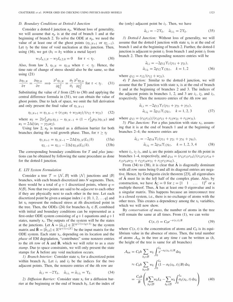
Depending on its location and size, a void might lead toan EF. Specifically, if a large enough void forms below a via,it might in some cases cause an open circuit failure by dis-connecting the via. This happens because the capping layeris not conductive; hence if the void covers the entire crosssection of a via, there is no conductive path left between thevia and the tree below and the current in the via completely
1322 IEEE TRANSACTIONS ON COMPUTER-AIDED DESIGN OF INTEGRATED CIRCUITS AND SYSTEMS, VOL. 37, NO. 7, JULY 2018
Fig. 4. EFs and conventional failures.
falls to 0, as shown in Fig. 4. On the other hand, voids thatform above the via generally happen at the top of the lineaway from the via, and so take a long time to completely fillthe cross section, and even then do not translate to an opencircuit because the current can continue to flow through themetal liner. Removal of a via, as it happens during the EFs, canhave a significant impact on grid reliability and thus shouldbe accounted for. In our model, once we have determined thesteady state void volume using (18), we check 1) if the voidis located below a via (this is determined based on geometryof the grid) and 2) if the void is large enough to disconnectthe via. If both conditions are met, this void leads to an EF,so that we remove the via from the power grid and update thevoltage drops and current density values.
IV. SOLVING THE EXTENDED MODEL
In this section, we will describe our approach for solving theextended Korhonen’s model for trees. First, for points withina branch, we will use the MoLs to convert the PDEs into a setof ODEs. Then, using the laws proposed in Section III-D, wewill derive the boundary conditions at the junctions. Finally,we merge the two and state the LTI system formulation thatdescribes the stress evolution for a given tree.
A. Scaling Korhonen’s Model
Korhonen’s model (2) is often scaled by introducing dimen-sionless variants of stress, length, and time [18]. This leads tostable PDEs that are easier to solve numerically. We definethe following scaling factors for any branch bk ∈ B:
τ= B�
kbTm
Dat
L2c
, ηk= �σk
kbTm
, ξk= xk
Lk(19)
where Da is the atomic diffusivity at some chosen nominal
temperature Tm, Lc is some chosen characteristic length and
0 ≤ xk ≤ Lk. The new variables τ , η, and ξ are referred toas reduced time, stress, and distance, respectively. Using (19)in (2) and applying the chain-rule, we get
∂ηk
∂τ= θk
∂
∂ξk
(∂ηk
∂ξk− αk
)(20)
where θk = (L2cDa,kT
m/L2kD
aTm,k), αk = (q∗ρjkLk/kbTm), jk
is the current density, Tm,k is the temperature, and Da,k is thediffusivity for bk. Since, for any given branch, αk is not afunction of distance ξk, then ∂αk/∂ξk = 0 and we get
∂ηk
∂τ= θk
∂2ηk
∂ξ2k
. (21)
For any branch bk, (21) constitutes the scaled PDE system tobe solved. Also, the atomic flux in bk can be restated in termsof reduced variables
Ja,k = Da,kCTm
LkTm,k
(∂ηk
∂ξk− αk
). (22)
B. Discretization for Tree Branch
We uniformly discretize branch bk into N segments, whereN is the same for all branches [because we have scaled allbranch lengths to 1 as in (19)]. The reduced stress at each ofthe N + 1 discrete spatial points {0, . . . N} is denoted by ηk,iand the time rate of change of ηk,i is [from (21)]
∂ηk,i
∂τ= θk
∂2ηk,i
∂ξ2k
for i = 0, 1, . . . , N. (23)
Further, we approximate the partial derivatives with respect toξ using central difference approximation, so that (23) leads to
dηk,i
dτ= θk
(ηk,i+1 + ηk,i−1 − 2ηk,i
(�ξ)2
)(24)
where �ξ = �ξk = 1/N, ∀k. The corresponding atomic fluxJa,k,i at the ith point is
Ja,k,i = Da,kCTm
LkTm,k
(ηk,i+1 − ηk,i−1
2�ξ− αk
). (25)
Note that for each branch, the ODEs at junctions (i = {0, N})require the values for ηk,−1 and ηk,N+1, which are not part ofthe ξk domain. The values at these ghost points are obtainedby solving for the respective boundary condition(s), as we nextexplain.
In order to simplify the presentation going forward, wedefine the following for any two branches bi, bk ∈ B:
rik = Li/Lk, pik = Da,iTm,k/(Da,kTm,i)
wik = wi/wk, γik = rkiwikpik, ϒk = θk/(�ξ)2. (26)
C. Boundary Conditions at Diffusion Barrier
Consider a diffusion barrier np connected to branch bk. Wehave two cases, one where np is at the predecessor junction(ξk = 0, start of the branch) and one where it is at the successorjunction (ξk = 1, branch end). We first obtain the bound-ary conditions for np at ξk = 0. Let τf be the time of voidnucleation at this barrier. Then, the corresponding boundarycondition is [using (16) and (17)]
∂ηk,0
∂ξk=
{αk τ < τfηk,0(Lk/δ) τ ≥ τf
(27)
where ηk,0 corresponds to σk,p in (17), with ηk,0 = ηth =(�σth)/(kbT
m) at τ = τf .Using the central difference approximation, we get
ηk,−1 ={
ηk,1 − 2�ξαk τ < τfηk,1 − 2�ξηk,0(Lk/δ) τ ≥ τf .
(28)
Similarly, for a diffusion barrier at ξk = 1, we get
ηk,N+1 ={
ηk,N−1 + 2�ξαk τ < τfηk,N−1 − 2�ξηk,N(Lk/δ) τ ≥ τf .
(29)
CHATTERJEE et al.: POWER GRID EM CHECKING USING PHYSICS-BASED MODELS 1323
D. Boundary Conditions at Dotted-I Junction
Consider a dotted-I junction np. Without loss of generality,we will assume that np is at the end of branch 1 and at thebeginning of branch 2. To solve the ODE at np, we need thevalue of at least one of the ghost points (η1,N+1 or η2,−1).Let τf be the time of void nucleation at this junction. Then,using (16), we get (h1 = h2 within a metal layer)
w1Ja,1,N − w2Ja,2,0 = 0 for τ < τf . (30)
Also, from law 3, η1,N = η2,0 when τ < τf . Hence, thetime rate of change of stress should also be the same, so thatusing (21)
∂η1,N
∂τ= ∂η2,0
∂τ=⇒ ∂2η1,N
∂ξ21
= θ2
θ1
∂2η2,0
∂ξ22
for τ < τf . (31)
Substituting the value of J from (25) to (30) and applying thecentral difference formula in (31), we can obtain the value ofghost points. Due to lack of space, we omit the full derivationand only present the final value of η1,N+1
η1,N+1 = η1,N−1 + (r12u1 + w21u2)/(r12 + w21) (32)
where u2 = 2(r212p21η2,1 − η1,N−1 + (1 − r2
12p21)η1,N) andu1 = 2�ξ(α1 − γ21α2).
Using law 2, np is treated as a diffusion barrier for bothbranches during the void growth phase. Thus, for τ ≥ τf
η1,N+1 = η1,N−1 − 2�ξη1,N(L1/δ) (33a)
η2,−1 = η2,1 − 2�ξη2,0(L2/δ). (33b)
The corresponding boundary conditions for T and plus junc-tions can be obtained by following the same procedure as donefor the dotted-I junction.
E. LTI System Formulation
Consider a tree T = {N ,B} with |N | junctions and |B|branches, with each branch discretized into N segments. Then,there would be a total of q + 1 discretized points, where q =N|B|. Note that two points are said to be adjacent to each otherif they are physically next to each other in the tree. Let eachdiscretized point be given a unique index i ∈ {0, 1, 2, . . . q} andlet xi represent the reduced stress at ith discretized point inthe tree. Then, the ODEs (24) for branches bk ∈ B, combinedwith initial and boundary conditions can be represented as afirst-order ODE system consisting of q+1 equations and q+1states, namely xi. The outputs of the system will be the statesat the junctions. Let A = [ai,k] ∈ R
(q+1)×(q+1) be the systemmatrix and B = [bi,k] ∈ R
(q+1)×|N | be the input matrix for theODE system. Each state xi, depending on its location and thephase of EM degradation, “contributes” some nonzero entriesto the ith row of A and B, which we will refer to as a statestamp. Due to space constraints, we will only present the statestamps for A before any void nucleation occurs.
1) Branch Interior: Consider state xi for a discretized pointwithin branch bk. Let i1 and i2 be the indices for the twoadjacent points. Then, the nonzero entries of the ith row are
ai,i = −2ϒk, ai,i1 = ai,i2 = ϒk. (34)
2) Diffusion Barrier: Consider state xi for a diffusion bar-rier at the beginning or the end of branch bk. Let the index of
the (only) adjacent point be i1. Then, we have
ai,i = −2ϒk, ai,i1 = 2ϒk. (35)
3) Dotted-I Junction: Without loss of generality, we willassume that the dotted-I junction with state xi is at the end ofbranch 1 and at the beginning of branch 2. Further, the dotted-Ijunction is adjacent to point i1 from branch 1 and point i2 frombranch 2. Then the corresponding nonzero entries will be
ai,i = −2�12ϒ1(γ11 + γ21),
ai,ik = 2�12ϒ1γk1, k = 1, 2 (36)
where �12 = r12/(r12 + w21).4) T Junction: Similar to the dotted-I junction, we will
assume that the T junction with state xi is at the end of branch1 and at the beginning of branches 2 and 3. The indices ofthe adjacent points in branches 1, 2, and 3 are i1, i2, and i3,respectively. Then the nonzero entries of the ith row are
ai,i = −2�13ϒ1(γ11 + γ21 + γ31),
ai,ik = 2�13ϒ1γk1, k = 1, 2, 3 (37)
where �13 = (r12r13)/(r12r13 + r13w21 + r12w31).5) Plus Junction: For a plus junction with state xi, assum-
ing that it is at the end of branch 1 and at the beginning ofbranches 2–4; the nonzero entries are
ai,i = −2�14ϒ1(γ11 + γ21 + γ31 + γ41),
ai,ik = 2�14ϒ1γk1, k = 1, 2, 3, 4 (38)
where i1, i2 i3, and i4 are the points adjacent to the ith point inbranches 1–4, respectively, and �14 = (r12r13r14)/(r12r13r14 +r13r14w21 + r12r14w31 + r12r13w41).
From (34) to (38), it is clear that A is diagonally dominantwith all row sums being 0 and all its diagonal entries are nega-tive. Hence, by Gershgorin circle theorem [23], all eigenvaluesof A must lie in the left half of the complex plane. Also, byconstruction, we have Az = 0 for z = [1 1 . . . 1]T or amultiple thereof. Thus, A has at least one 0 eigenvalue and isa singular matrix. This happens because an interconnect treeis a closed system, i.e., there is no exchange of atoms with theother trees. This creates a dependency among the xi variables,which we will now show.
By conservation of mass, the number of atoms in the treewill remain the same at all times. From (1), we can write
C(x, t) = C0e−σ(x,t)/B (39)
where C(x, t) is the concentration of atoms and C0 is its equi-librium value in the absence of stress. Then, the total numberof atoms Atot in the tree at any time t can be written as (h,the height of the tree is same for all branches)
Atot = C0h∑
bk∈Bwk
∫ Lk
0e−σk(xk,t)/B dxk
≈ C0h∑
bk∈Bwk
∫ Lk
0(1 − σk(xk, t)/B) dxk
= C0h
B
⎛
⎝B∑
bk∈BwkLk −
∑
bk∈Bwk
∫ Lk
0σk(xk, t) dxk
⎞
⎠ (40)
1324 IEEE TRANSACTIONS ON COMPUTER-AIDED DESIGN OF INTEGRATED CIRCUITS AND SYSTEMS, VOL. 37, NO. 7, JULY 2018
where we used the approximation ex ≈ 1 + x for x � 1because σk(xk, t) � B, ∀t. Clearly, only the stress values inthe second summation term in (40) change with time; every-thing else remains constant. Therefore, the tensile/compressivestresses generated by the movement of atoms can only varyin a way that satisfies the conservation of mass. Define
β(τ) �∑
bk∈BwkLk
∫ 1
0ηk(ξk, τ )dξk (41)
which is the second summation term in (40) rewritten in termsof the reduced stress. Since the stress values for all points atτ = 0 is known from initial conditions, β(0) = β0 is always aknown quantity. Then, in order to satisfy the conservation ofmass, we must have β(0) = β(τ) ∀τ . Evaluating the integralin (41) using the trapezoidal rule, we can write
β0 =q∑
i=0
cixi(τ ) (42)
where ci are the coefficients as determined by the trapezoidalrule. This gives us a linear dependence between xi so that onestate can be eliminated. Without loss of generality, let x0 bea nonoutput state to be eliminated. Define
x(τ ) �[x1(τ ) x2(τ ) . . . xq−1(τ ) xq(τ )
]T (43)
to be the state vector. Now, we can write
x0(τ ) = −cTx(τ ) + β0/
c0 (44)
where c = c−10 [ c1 c2 . . . cq ]T ∈R
q. Using (44) and theprevious ODE formulation, we can eliminate x0 from the ODEequations (thereby removing the eigenvalue at 0) so that thestress evolution in a tree can be represented by an LTI systemwith q ODE equations with q independent states:
x(τ ) = Ax(τ ) + Bu (45a)
y(τ ) = Lx(τ ) (45b)
x(0) = [ηT,1(0) ηT,2(0) . . . ηT,q(0)
](45c)
where ηT,i(0) is the reduced thermal stress at t = 0 at the ithdiscretized point, u ∈ R
|N | is the input vector which dependson the branch current densities, A ∈ R
q×q is the system matrixand B ∈ R
q×|N | is the input matrix such that
A = −aqcT + Aq (46a)
B = Bq + (β0/c0)aquT , u ∈ R|N | and uT · u = 1 (46b)
with aq = [ai,k] for 1 ≤ i ≤ q, k = 0, Aq = [ai,k] for1 ≤ i, k ≤ q and Bq = [bi,k] for 1 ≤ i ≤ q, 0 ≤ k ≤ |N | − 1.The output y(τ ) ∈ R
|N | is the vector of stress values at thejunctions and L ∈ R
|N |×q is the output matrix.Between any two void nucleations, A, B and input u are
constant. Hence, we can further simplify the LTI systemrepresentation by applying the following change of variables:
x(τ ) = x(τ ) − xss (47)
where xss = −A−1Bu is the steady state stress of the tree forthe given input u. Finally, we can rewrite (45) as
˙x(τ ) = Ax(τ ) (48a)
(a) (b)
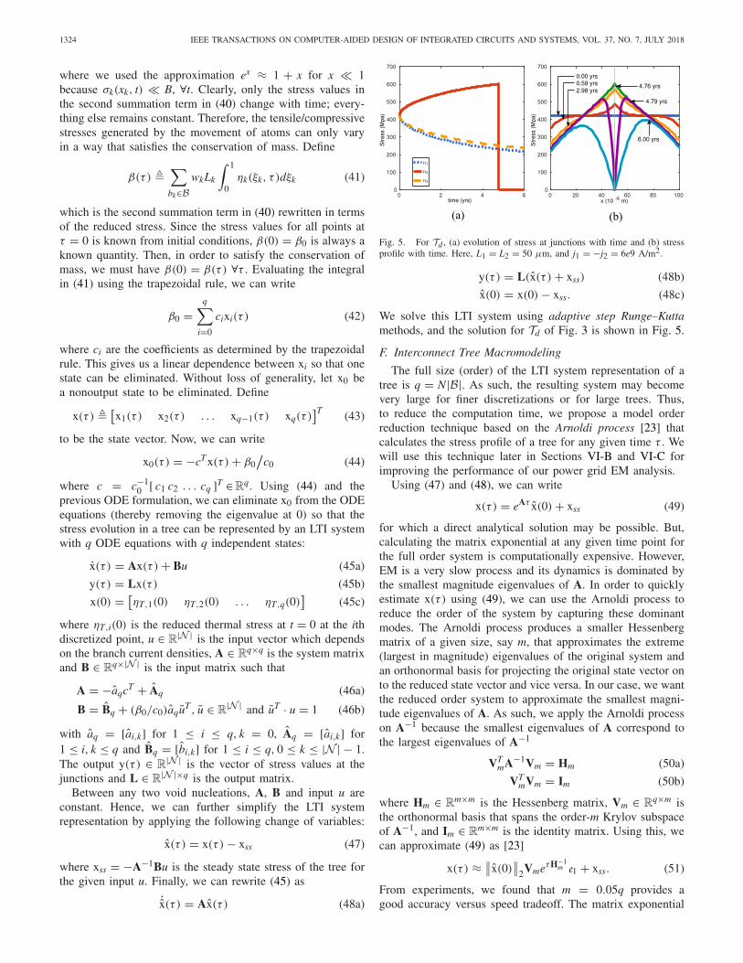
Fig. 5. For Td , (a) evolution of stress at junctions with time and (b) stressprofile with time. Here, L1 = L2 = 50 μm, and j1 = −j2 = 6e9 A/m2.
y(τ ) = L(x(τ ) + xss) (48b)
x(0) = x(0) − xss. (48c)
We solve this LTI system using adaptive step Runge–Kuttamethods, and the solution for Td of Fig. 3 is shown in Fig. 5.
F. Interconnect Tree Macromodeling
The full size (order) of the LTI system representation of atree is q = N|B|. As such, the resulting system may becomevery large for finer discretizations or for large trees. Thus,to reduce the computation time, we propose a model orderreduction technique based on the Arnoldi process [23] thatcalculates the stress profile of a tree for any given time τ . Wewill use this technique later in Sections VI-B and VI-C forimproving the performance of our power grid EM analysis.
Using (47) and (48), we can write
x(τ ) = eAτ x(0) + xss (49)
for which a direct analytical solution may be possible. But,calculating the matrix exponential at any given time point forthe full order system is computationally expensive. However,EM is a very slow process and its dynamics is dominated bythe smallest magnitude eigenvalues of A. In order to quicklyestimate x(τ ) using (49), we can use the Arnoldi process toreduce the order of the system by capturing these dominantmodes. The Arnoldi process produces a smaller Hessenbergmatrix of a given size, say m, that approximates the extreme(largest in magnitude) eigenvalues of the original system andan orthonormal basis for projecting the original state vector onto the reduced state vector and vice versa. In our case, we wantthe reduced order system to approximate the smallest magni-tude eigenvalues of A. As such, we apply the Arnoldi processon A−1 because the smallest eigenvalues of A correspond tothe largest eigenvalues of A−1
VTmA−1Vm = Hm (50a)
VTmVm = Im (50b)
where Hm ∈ Rm×m is the Hessenberg matrix, Vm ∈ R
q×m isthe orthonormal basis that spans the order-m Krylov subspaceof A−1, and Im ∈ R
m×m is the identity matrix. Using this, wecan approximate (49) as [23]
x(τ ) ≈ ∥∥x(0)
∥∥
2VmeτH−1m e1 + xss. (51)
From experiments, we found that m = 0.05q provides agood accuracy versus speed tradeoff. The matrix exponential
CHATTERJEE et al.: POWER GRID EM CHECKING USING PHYSICS-BASED MODELS 1325
in (51) is calculated using the scaling and squaringmethod [23]. In practice, this approximation can be computedquickly because m � q, and thus can be used to obtain thestress profile of a tree at any given time.
V. DETERMINING BRANCH TEMPERATURES
Accounting for the temperature distribution across the layerswhile doing EM analysis is very important due to three rea-sons. First, the initial residual stress at t = 0 for any given treeis mainly due to the thermal stress, which is strongly depen-dent on the initial temperature [see (9)]. Second, from (4),the diffusivity of branch bk, which determines the time rateof change of stress, depends on its temperature Tm,k. Finally,the steady state void length depends on thermal stress: higherthermal stress leads to larger voids. As such, to perform real-istic EM checking, one needs to determine the temperaturedistribution for different layers in the grid. We do this usingprevious work [24], [25], which we will summarize briefly forcompleteness.
A. Thermal Modeling
Each layer in the power grid is discretized into uniform vol-ume elements called thermal blocks [24]. Each thermal blockrepresents an isothermal volume within a layer, and as such allbranches and junctions that reside within a thermal block havethe same temperature. For simplicity, we assume that a givenbranch cannot span two thermal blocks, so that it has no tem-perature gradient. For each block, we perform thermal analysisusing compact thermal modeling (CTM) [25] based on electro-thermal equivalence. A CTM is a lumped thermal RC network,with heat dissipation modeled as a current source. Specifically,each thermal block is represented as a thermal node connectedto six resistors, a current source, and a capacitor. The resistorsmodel the heat conductivity to neighboring blocks and theirvalues are determined using thermal properties and geometryof the thermal block
gE/W = 2k effbwbh/bl, gN/S = 2k effblbh/bw
gup/down = 2k effblbw/bh (52)
where k eff is the effective thermal conductivity and eachthermal block has dimension bl×bw×bh. The total power dis-sipated in a thermal block can be written as P = Pself_heating +Plogic, where Pself_heating is due to the average power dissi-pated by joule heating of the metal branches within the thermalblock and Plogic is the average heat dissipated by the underly-ing logic, due to active switching and leakage currents. Notethat Plogic contributes to power dissipation of thermal nodesin the lowest layer only. In our case, we are only interestedin the steady state temperature distribution because transientsin temperature occur on a time scale that is small when com-pared to the EM. Thus, we ignore the thermal capacitance anduse the steady state temperature distribution in our analysis.
The number of thermal blocks per layer is the same andis decided based on the required resolution for temperaturedistribution. In addition, we assume convective boundary con-dition [24] at the top and insulated boundary conditions at thefour sides to model the heat transfer between the power gridand the surroundings. The CTMs for thermal blocks, combined
with the boundary conditions, gives us a thermal grid that canbe solved for finding the temperature distribution of the powergrid. We generate the thermal grid at t = 0 and calculate theinitial temperature distribution to find the residual stress andthe branch diffusivities. After a void nucleates, the branch cur-rents change. Hence, we update the Pself_heating for all thermalnodes, find the new temperature distribution and update thebranch diffusivities.
VI. POWER GRID EM ANALYSIS
Because EM is a long-term failure mechanism, short-termtransients that may be typically experienced in chip work-loads do not play a significant role in EM degradation. Hence,and consistent with standard practice in the field, we usean effective-current model [26], so that the grid currents areassumed to be constant at some average (effective) value, atleast during the void nucleation phase. Once a void nucle-ates, branch resistances change fairly quickly and the currentschange, also fairly quickly, to new effective values. Thus,between any two successive void nucleations, the grid hasfixed currents, voltages, and conductances and so can be mod-eled using a dc model. To denote the fact that conductances(and the corresponding voltages) change from one nucleationphase to the next, as in [8], we express the grid model as
G(t)v(t) = is (53)
where G(t) is the time-varying (but piecewise-constant) con-ductance matrix, v(t) is the corresponding time-varying (butpiecewise constant) vector of node voltage drops, and is is thevector of effective values of the current sources tied to thegrid.
A. Main Approach
As explained earlier, we use the mesh model to find theMTF, in which the grid is deemed to fail not when the firstvoid has nucleated, but when enough voids have nucleated sothat the voltage drop specification has exceeded at some gridnode. As a byproduct, however, this process also produces thetime when the first void nucleates, which helps us generatethe MTF under a series model, in which a grid is deemed tofail when the first void nucleates. We report the series modelMTF for comparison purposes.
We assume that the grid is undamaged (no voids) at t = 0.A voltage-drop threshold value for every grid node (or a sub-set of grid nodes) is given, which is captured in the vectorvth. Initially, all node voltage drops are less than vth, i.e.,v(0) < vth. A power grid is a collection of interconnect trees.As such, to estimate the EM degradation of the grid, we for-mulate the LTI system for every tree as shown in Section IV-Eand numerically integrate it to obtain the stress as a functionof position and time. Every time a void nucleates at a junction(i.e., the stress reaches σth), we pause the integration, calcu-late the steady state volume of the void and update the branchresistances and current density values. We then check to seeif this void leads to an EF, and if it does, we remove the cor-responding via from the power grid and update the voltagedrops. Then, we determine the new temperature distributionof the grid, update the corresponding boundary conditions and
1326 IEEE TRANSACTIONS ON COMPUTER-AIDED DESIGN OF INTEGRATED CIRCUITS AND SYSTEMS, VOL. 37, NO. 7, JULY 2018
(a) (b)
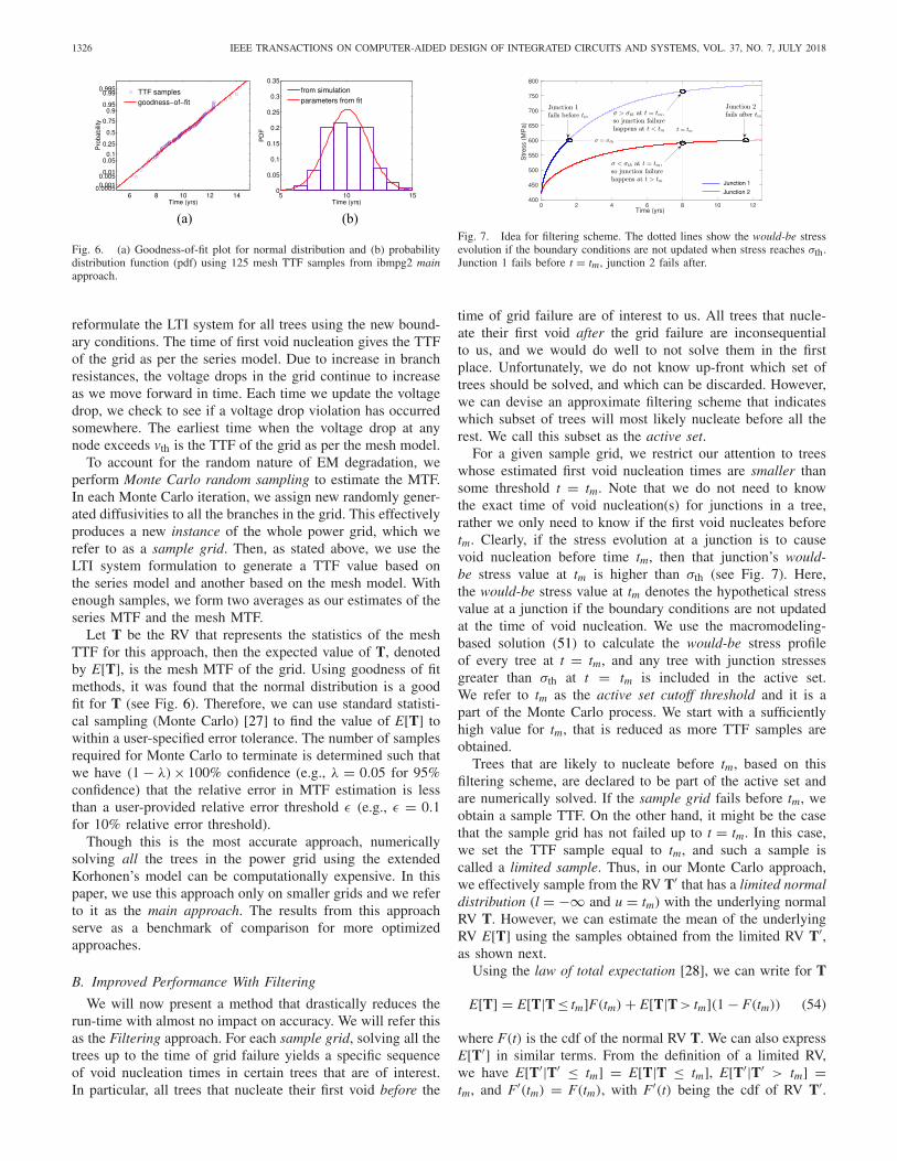
Fig. 6. (a) Goodness-of-fit plot for normal distribution and (b) probabilitydistribution function (pdf) using 125 mesh TTF samples from ibmpg2 mainapproach.
reformulate the LTI system for all trees using the new bound-ary conditions. The time of first void nucleation gives the TTFof the grid as per the series model. Due to increase in branchresistances, the voltage drops in the grid continue to increaseas we move forward in time. Each time we update the voltagedrop, we check to see if a voltage drop violation has occurredsomewhere. The earliest time when the voltage drop at anynode exceeds vth is the TTF of the grid as per the mesh model.
To account for the random nature of EM degradation, weperform Monte Carlo random sampling to estimate the MTF.In each Monte Carlo iteration, we assign new randomly gener-ated diffusivities to all the branches in the grid. This effectivelyproduces a new instance of the whole power grid, which werefer to as a sample grid. Then, as stated above, we use theLTI system formulation to generate a TTF value based onthe series model and another based on the mesh model. Withenough samples, we form two averages as our estimates of theseries MTF and the mesh MTF.
Let T be the RV that represents the statistics of the meshTTF for this approach, then the expected value of T, denotedby E[T], is the mesh MTF of the grid. Using goodness of fitmethods, it was found that the normal distribution is a goodfit for T (see Fig. 6). Therefore, we can use standard statisti-cal sampling (Monte Carlo) [27] to find the value of E[T] towithin a user-specified error tolerance. The number of samplesrequired for Monte Carlo to terminate is determined such thatwe have (1 − λ)× 100% confidence (e.g., λ = 0.05 for 95%confidence) that the relative error in MTF estimation is lessthan a user-provided relative error threshold ε (e.g., ε = 0.1for 10% relative error threshold).
Though this is the most accurate approach, numericallysolving all the trees in the power grid using the extendedKorhonen’s model can be computationally expensive. In thispaper, we use this approach only on smaller grids and we referto it as the main approach. The results from this approachserve as a benchmark of comparison for more optimizedapproaches.
B. Improved Performance With Filtering
We will now present a method that drastically reduces therun-time with almost no impact on accuracy. We will refer thisas the Filtering approach. For each sample grid, solving all thetrees up to the time of grid failure yields a specific sequenceof void nucleation times in certain trees that are of interest.In particular, all trees that nucleate their first void before the
Fig. 7. Idea for filtering scheme. The dotted lines show the would-be stressevolution if the boundary conditions are not updated when stress reaches σth.Junction 1 fails before t = tm, junction 2 fails after.
time of grid failure are of interest to us. All trees that nucle-ate their first void after the grid failure are inconsequentialto us, and we would do well to not solve them in the firstplace. Unfortunately, we do not know up-front which set oftrees should be solved, and which can be discarded. However,we can devise an approximate filtering scheme that indicateswhich subset of trees will most likely nucleate before all therest. We call this subset as the active set.
For a given sample grid, we restrict our attention to treeswhose estimated first void nucleation times are smaller thansome threshold t = tm. Note that we do not need to knowthe exact time of void nucleation(s) for junctions in a tree,rather we only need to know if the first void nucleates beforetm. Clearly, if the stress evolution at a junction is to causevoid nucleation before time tm, then that junction’s would-be stress value at tm is higher than σth (see Fig. 7). Here,the would-be stress value at tm denotes the hypothetical stressvalue at a junction if the boundary conditions are not updatedat the time of void nucleation. We use the macromodeling-based solution (51) to calculate the would-be stress profileof every tree at t = tm, and any tree with junction stressesgreater than σth at t = tm is included in the active set.We refer to tm as the active set cutoff threshold and it is apart of the Monte Carlo process. We start with a sufficientlyhigh value for tm, that is reduced as more TTF samples areobtained.
Trees that are likely to nucleate before tm, based on thisfiltering scheme, are declared to be part of the active set andare numerically solved. If the sample grid fails before tm, weobtain a sample TTF. On the other hand, it might be the casethat the sample grid has not failed up to t = tm. In this case,we set the TTF sample equal to tm, and such a sample iscalled a limited sample. Thus, in our Monte Carlo approach,we effectively sample from the RV T′ that has a limited normaldistribution (l = −∞ and u = tm) with the underlying normalRV T. However, we can estimate the mean of the underlyingRV E[T] using the samples obtained from the limited RV T′,as shown next.
Using the law of total expectation [28], we can write for T
E[T] = E[T|T ≤ tm]F(tm) + E[T|T > tm](1 − F(tm)) (54)
where F(t) is the cdf of the normal RV T. We can also expressE[T′] in similar terms. From the definition of a limited RV,we have E[T′|T′ ≤ tm] = E[T|T ≤ tm], E[T′|T′ > tm] =tm, and F′(tm) = F(tm), with F′(t) being the cdf of RV T′.
CHATTERJEE et al.: POWER GRID EM CHECKING USING PHYSICS-BASED MODELS 1327
Hence, we can write
E[T′] = E[T|T ≤ tm]F(tm) + tm(1 − F(tm)). (55)
Subtracting (55) from (54), we get
E[T] = E[T′] + (E[T|T > tm] − tm)(1 − F(tm))
= E[T′] + E[T − tm|T > tm](1 − F(tm)). (56)
The term E[T− tm|T > tm] is the mean residual life (MRL) ofthe power grid at t = tm. Define μ � E[T], μ′ � E[T′], andpf � F(tm). Since we know that T has a normal distribution,the MRL of the power grid at t = tm can be expressed in termsof μ and pf . From (56), after some algebraic manipulation, weobtain
μ = μ′ + (κ − 1)tmκ
(57)
where κ = pf + φ(�−1(pf ))/�−1(pf ), �(t) and φ(t) are,respectively, the cdf and pdf of a standard normal distributionN (0, 1). �−1 denotes the inverse cdf of N (0, 1) which canbe computed on most operating systems using the erfinv()function. We estimate μ′ and pf from the statistical samplingprocess. Let {T ′
1, T ′2, . . . T ′
s} be s samples obtained from RVT′ using a Monte Carlo process. Then, define
μ′ � 1
s
s∑
k=1
T ′k, pf � 1 −
∣∣{T ′k : T ′
k > tm}∣∣
s(58)
where μ′ is the estimated value of μ′ and pf is the estimatedvalue of pf . Thus, using μ′ and pf in (57) we can calculateμ, the estimated value of μ. Note that μ′, pf , and μ are thetrue values, so that lims→∞ μ′ = μ′, lims→∞ pf = pf , andlims→∞ μ = μ. Then, the error in estimation can be writtenas: δμ = |μ − μ|, δμ′ = |μ′ − μ′|, and δpf = |pf − pf |.
Similar to the main approach, we stop the Monte Carloprocess when we are (1−λ)×100% confident that the rela-tive error in estimated MTF is less than some user providedthreshold ε. In other words, we stop if
δμλ
μ≤ ε ⇐⇒ δμλ
μ≤ ε
1 + ε(59)
where δμλ is (1−λ) × 100% confidence bound on the esti-mation error δμ. In other words, this means that the interval[μ − δμλ, μ + δμλ] will contain μ (the true value) (1 − λ) ×100% of the time. Using propagation of errors [29] in (57),we get
δμλ =√(
∂μ
∂μ′ δμ′λ
)2
+(
∂μ
∂pfδpf λ
)2
(60)
where δμ′λ and δpf λ are the (1−λ)×100% confidence bounds
on μ′ and pf , respectively. δμ′λ is obtained from simulation,
using the technique given in [21] and δpf λ can be calculatedfrom the TTF samples using [30]. For lack of space, we skipthe details and present the final expression
δμ2λ = (δμ′
λ)2
κ2
+ z2λ/2(tm − μ′)2pf (1 − pf )
κ4s
[
1 +(
1 + 1
y2
)2]
(61)
TABLE ICOMPARISON OF POWER GRID MTF USING THE
MAIN APPROACH AND FILTERING APPROACH
where zλ/2 is the (1 − λ/2)-percentile of N (0, 1), κ = pf +φ(y)/y and y = �−1(pf ). We obtain at least 30 TTF samplesbefore starting to check the stopping criteria (59).
C. TTF Predictor Approach
We next describe a predictor-based approach to furtherspeed up the MTF computation. This approach is applied ontop of the filtering approach explained earlier and gives excel-lent speed-ups. It makes use of the reduced-order model givenin Section IV-F earlier.
Once the stress profile of a tree is determined for a fewtime-points using (51), it should be possible to extrapolate therest of the trend, with some suitably nonlinear fitting function.The fitting function can thus be used as a TTF predictor, tofind a good estimate of the nucleation times for all junctionswithin the tree. Parameters of the function can be found usingleast-squares fitting, based on the points already solved. Whilevarious exponential or log functions may be suitable, we havefound empirically that the following power function templateprovides a very good fit:
f (t) = atb+c ln t (62)
where a, b, and c are parameters to be determined using regres-sion analysis and least-squares fitting and f (t) is the stressvalue at time t. Note that ln(f (t)) is a simple quadratic in ln t,with ln a, b, and c as the three coefficients. Once we estimatethe time of void nucleations using (51) and the TTF predictor,we can predict the time (and sequence) of void nucleations.For each void nucleation, we update the corresponding branchresistances and voltage drops until the grid fails.
VII. EXPERIMENTAL RESULTS
All approaches have been implemented in C++ and testedon a number of IBM power grid benchmarks [16], usinga quad-core 3.4 GHz Linux machine with 32GB of RAM.The interconnect material is assumed to be copper, so thatthe following parameters are used in our EM model: B =1.35×10¹¹ Pa, � = 1.66×10⁻²⁹ m3, kb = 1.38×10⁻²³ J/K,q∗ = 8.0109 × 10⁻¹⁹ C, σth = 600 × 106 Pa [9], andδ = 10−9 m. An ambient temperature of 300 K is used forall simulations. Each branch is discretized into N = 16 seg-ments. We use a relative tolerance of 10−3 and an absolutetolerance of 10−6 for the ODE solver. For all grids, we usedλ = 0.05 (95% confidence bounds) and ε = 0.1 (maximumrelative error threshold of 10%). In our implementation, weuse a shared memory model to parallelize the computation.
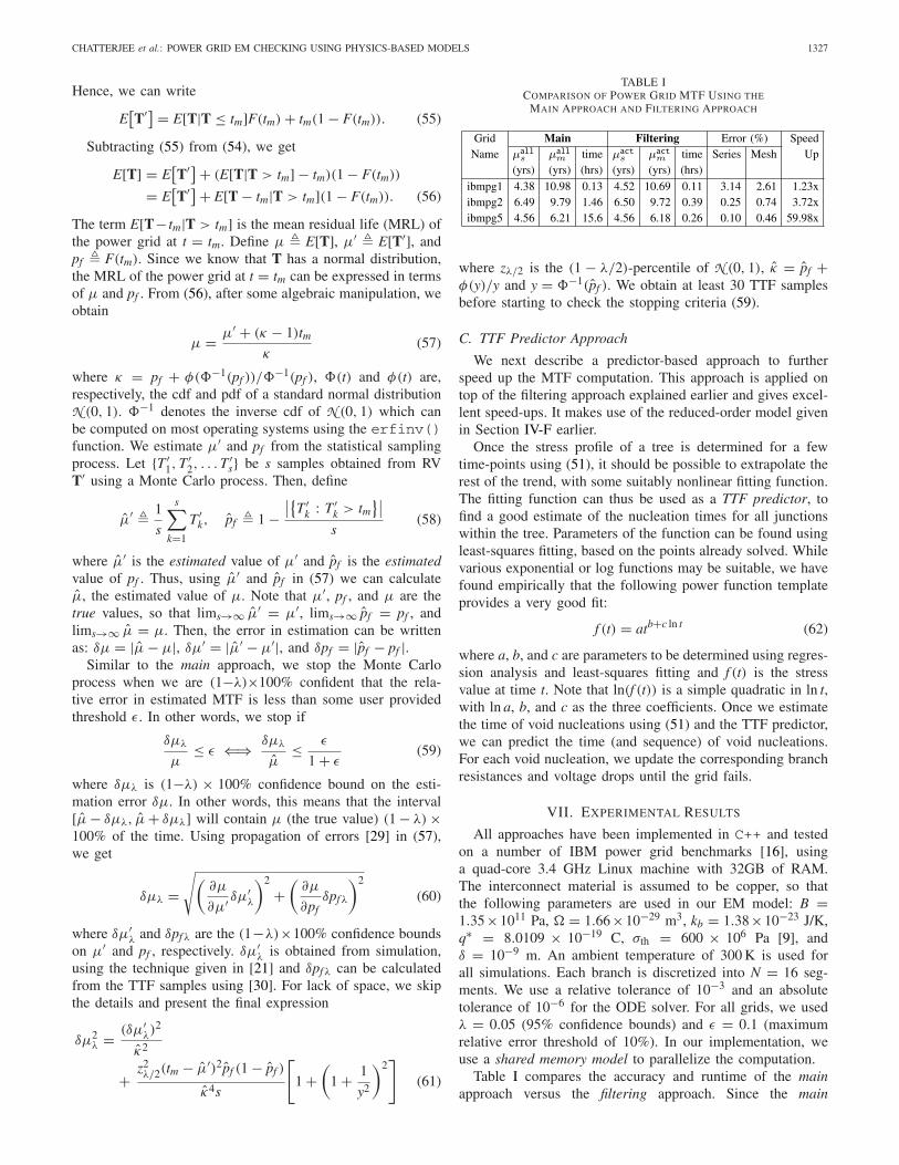
Table I compares the accuracy and runtime of the mainapproach versus the filtering approach. Since the main
1328 IEEE TRANSACTIONS ON COMPUTER-AIDED DESIGN OF INTEGRATED CIRCUITS AND SYSTEMS, VOL. 37, NO. 7, JULY 2018
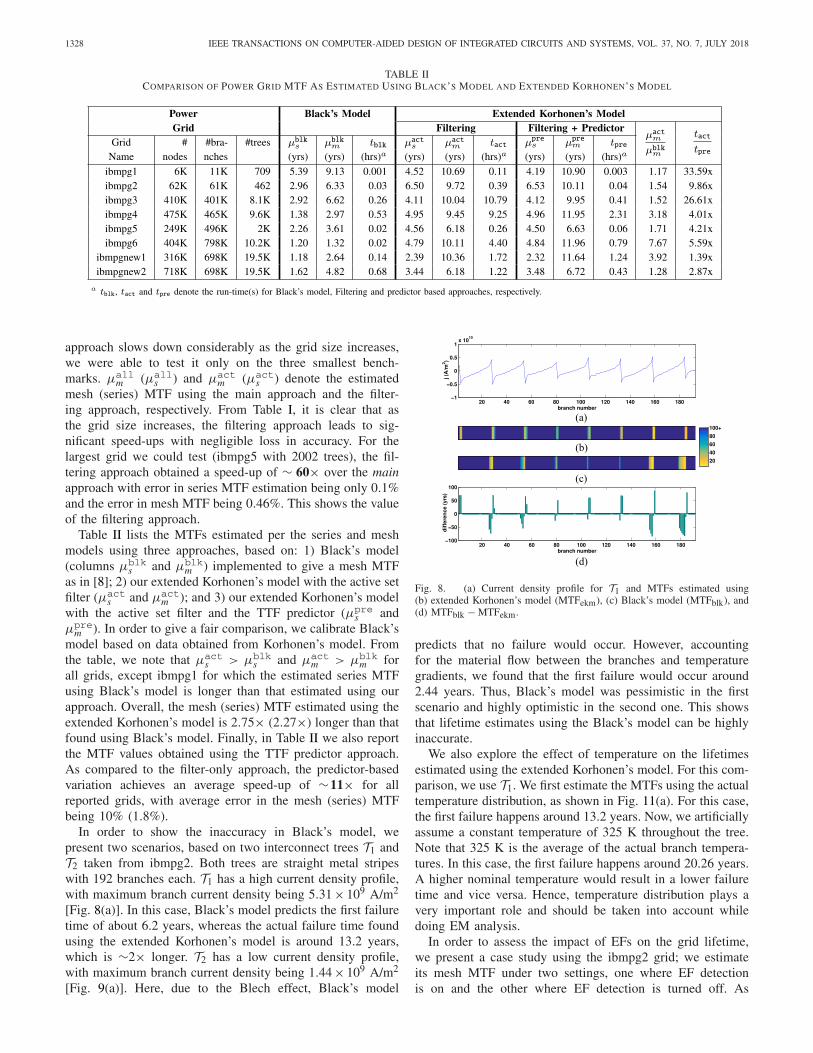
TABLE IICOMPARISON OF POWER GRID MTF AS ESTIMATED USING BLACK’S MODEL AND EXTENDED KORHONEN’S MODEL
approach slows down considerably as the grid size increases,we were able to test it only on the three smallest bench-marks. μall
m (μalls ) and μact
m (μacts ) denote the estimated
mesh (series) MTF using the main approach and the filter-ing approach, respectively. From Table I, it is clear that asthe grid size increases, the filtering approach leads to sig-nificant speed-ups with negligible loss in accuracy. For thelargest grid we could test (ibmpg5 with 2002 trees), the fil-tering approach obtained a speed-up of ∼ 60× over the mainapproach with error in series MTF estimation being only 0.1%and the error in mesh MTF being 0.46%. This shows the valueof the filtering approach.
Table II lists the MTFs estimated per the series and meshmodels using three approaches, based on: 1) Black’s model(columns μblk
s and μblkm ) implemented to give a mesh MTF
as in [8]; 2) our extended Korhonen’s model with the active setfilter (μact
s and μactm ); and 3) our extended Korhonen’s model
with the active set filter and the TTF predictor (μpres and
μprem ). In order to give a fair comparison, we calibrate Black’s
model based on data obtained from Korhonen’s model. Fromthe table, we note that μact
s > μblks and μact
m > μblkm for
all grids, except ibmpg1 for which the estimated series MTFusing Black’s model is longer than that estimated using ourapproach. Overall, the mesh (series) MTF estimated using theextended Korhonen’s model is 2.75× (2.27×) longer than thatfound using Black’s model. Finally, in Table II we also reportthe MTF values obtained using the TTF predictor approach.As compared to the filter-only approach, the predictor-basedvariation achieves an average speed-up of ∼11× for allreported grids, with average error in the mesh (series) MTFbeing 10% (1.8%).
In order to show the inaccuracy in Black’s model, wepresent two scenarios, based on two interconnect trees T1 andT2 taken from ibmpg2. Both trees are straight metal stripeswith 192 branches each. T1 has a high current density profile,with maximum branch current density being 5.31 × 10⁹ A/m2
[Fig. 8(a)]. In this case, Black’s model predicts the first failuretime of about 6.2 years, whereas the actual failure time foundusing the extended Korhonen’s model is around 13.2 years,which is ∼2× longer. T2 has a low current density profile,with maximum branch current density being 1.44 × 10⁹ A/m2
[Fig. 9(a)]. Here, due to the Blech effect, Black’s model
(a)
(b)
(c)
(d)
Fig. 8. (a) Current density profile for T1 and MTFs estimated using(b) extended Korhonen’s model (MTFekm), (c) Black’s model (MTFblk), and(d) MTFblk − MTFekm.
predicts that no failure would occur. However, accountingfor the material flow between the branches and temperaturegradients, we found that the first failure would occur around2.44 years. Thus, Black’s model was pessimistic in the firstscenario and highly optimistic in the second one. This showsthat lifetime estimates using the Black’s model can be highlyinaccurate.
We also explore the effect of temperature on the lifetimesestimated using the extended Korhonen’s model. For this com-parison, we use T1. We first estimate the MTFs using the actualtemperature distribution, as shown in Fig. 11(a). For this case,the first failure happens around 13.2 years. Now, we artificiallyassume a constant temperature of 325 K throughout the tree.Note that 325 K is the average of the actual branch tempera-tures. In this case, the first failure happens around 20.26 years.A higher nominal temperature would result in a lower failuretime and vice versa. Hence, temperature distribution plays avery important role and should be taken into account whiledoing EM analysis.
In order to assess the impact of EFs on the grid lifetime,we present a case study using the ibmpg2 grid; we estimateits mesh MTF under two settings, one where EF detectionis on and the other where EF detection is turned off. As
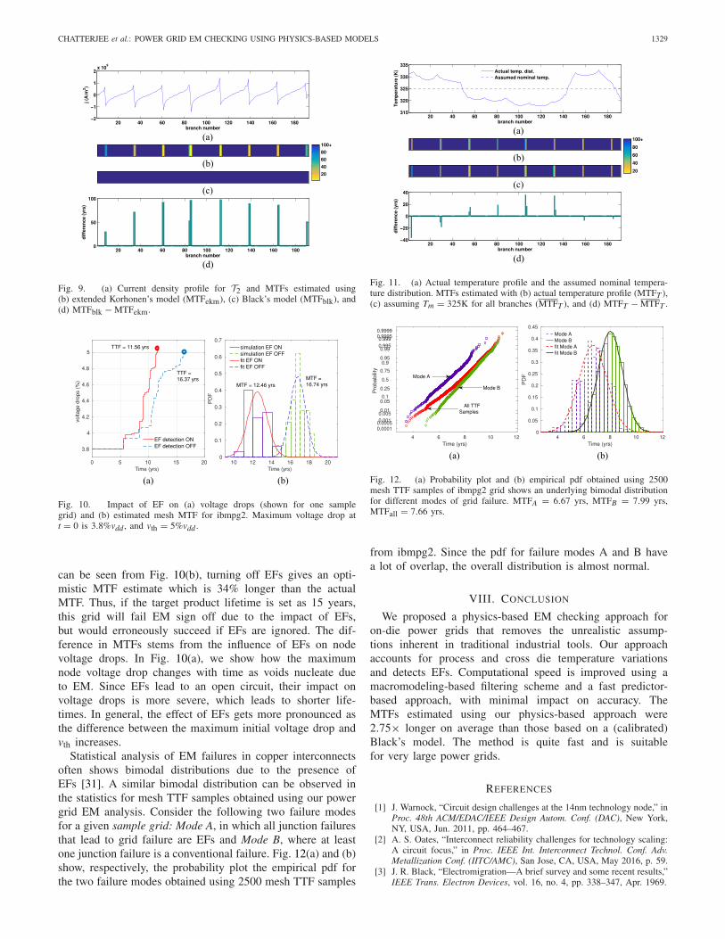
CHATTERJEE et al.: POWER GRID EM CHECKING USING PHYSICS-BASED MODELS 1329
(a)
(b)
(c)
(d)
Fig. 9. (a) Current density profile for T2 and MTFs estimated using(b) extended Korhonen’s model (MTFekm), (c) Black’s model (MTFblk), and(d) MTFblk − MTFekm.
(a) (b)
Fig. 10. Impact of EF on (a) voltage drops (shown for one samplegrid) and (b) estimated mesh MTF for ibmpg2. Maximum voltage drop att = 0 is 3.8%vdd , and vth = 5%vdd .
can be seen from Fig. 10(b), turning off EFs gives an opti-mistic MTF estimate which is 34% longer than the actualMTF. Thus, if the target product lifetime is set as 15 years,this grid will fail EM sign off due to the impact of EFs,but would erroneously succeed if EFs are ignored. The dif-ference in MTFs stems from the influence of EFs on nodevoltage drops. In Fig. 10(a), we show how the maximumnode voltage drop changes with time as voids nucleate dueto EM. Since EFs lead to an open circuit, their impact onvoltage drops is more severe, which leads to shorter life-times. In general, the effect of EFs gets more pronounced asthe difference between the maximum initial voltage drop andvth increases.
Statistical analysis of EM failures in copper interconnectsoften shows bimodal distributions due to the presence ofEFs [31]. A similar bimodal distribution can be observed inthe statistics for mesh TTF samples obtained using our powergrid EM analysis. Consider the following two failure modesfor a given sample grid: Mode A, in which all junction failuresthat lead to grid failure are EFs and Mode B, where at leastone junction failure is a conventional failure. Fig. 12(a) and (b)show, respectively, the probability plot the empirical pdf forthe two failure modes obtained using 2500 mesh TTF samples
(a)
(b)
(c)
(d)
Fig. 11. (a) Actual temperature profile and the assumed nominal tempera-ture distribution. MTFs estimated with (b) actual temperature profile (MTFT ),(c) assuming Tm = 325K for all branches (MTFT ), and (d) MTFT − MTFT .
(a) (b)
Fig. 12. (a) Probability plot and (b) empirical pdf obtained using 2500mesh TTF samples of ibmpg2 grid shows an underlying bimodal distributionfor different modes of grid failure. MTFA = 6.67 yrs, MTFB = 7.99 yrs,MTFall = 7.66 yrs.
from ibmpg2. Since the pdf for failure modes A and B havea lot of overlap, the overall distribution is almost normal.
VIII. CONCLUSION
We proposed a physics-based EM checking approach foron-die power grids that removes the unrealistic assump-tions inherent in traditional industrial tools. Our approachaccounts for process and cross die temperature variationsand detects EFs. Computational speed is improved using amacromodeling-based filtering scheme and a fast predictor-based approach, with minimal impact on accuracy. TheMTFs estimated using our physics-based approach were2.75× longer on average than those based on a (calibrated)Black’s model. The method is quite fast and is suitablefor very large power grids.
REFERENCES
[1] J. Warnock, “Circuit design challenges at the 14nm technology node,” inProc. 48th ACM/EDAC/IEEE Design Autom. Conf. (DAC), New York,NY, USA, Jun. 2011, pp. 464–467.
[2] A. S. Oates, “Interconnect reliability challenges for technology scaling:A circuit focus,” in Proc. IEEE Int. Interconnect Technol. Conf. Adv.Metallization Conf. (IITC/AMC), San Jose, CA, USA, May 2016, p. 59.
[3] J. R. Black, “Electromigration—A brief survey and some recent results,”IEEE Trans. Electron Devices, vol. 16, no. 4, pp. 338–347, Apr. 1969.

1330 IEEE TRANSACTIONS ON COMPUTER-AIDED DESIGN OF INTEGRATED CIRCUITS AND SYSTEMS, VOL. 37, NO. 7, JULY 2018
[4] M. Hauschildt et al., “Electromigration early failure void nucleationand growth phenomena in Cu and Cu(Mn) interconnects,” in Proc.IEEE Int. Rel. Phys. Symp. (IRPS), Anaheim, CA, USA, Apr. 2013,pp. 2C.1.1–2C.1.6.
[5] J. Lloyd, “Black’s law revisited—Nucleation and growth in electromi-gration failure,” Microelectron. Rel., vol. 47, nos. 9–11, pp. 1468–1472,2007.
[6] I. A. Blech, “Electromigration in thin aluminum films on titaniumnitride,” J. Appl. Phys., vol. 47, no. 4, pp. 1203–1208, 1976.
[7] C. L. Gan, C. V. Thompson, K. L. Pey, and W. K. Choi, “Experimentalcharacterization and modeling of the reliability of three-terminal dual-damascene Cu interconnect trees,” J. Appl. Phys., vol. 94, no. 2,pp. 1222–1228, 2003.
[8] S. Chatterjee, M. Fawaz, and F. N. Najm, “Redundancy-aware electromi-gration checking for mesh power grids,” in Proc. IEEE/ACM Int. Conf.Comput.-Aided Design, San Jose, CA, USA, Nov. 2013, pp. 540–547.
[9] X. Huang, Y. Tan, V. Sukharev, and S. X.-D. Tan, “Physics-basedelectromigration assessment for power grid networks,” in Proc.ACM/EDAC/IEEE Design Autom. Conf., San Francisco, CA, USA,Jun. 2014, pp. 1–6.
[10] M. A. Korhonen, P. Borgesen, K. N. Tu, and C.-Y. Li, “Stress evolutiondue to electromigration in confined metal lines,” J. Appl. Phys., vol. 73,no. 8, pp. 3790–3799, 1993.
[11] S. P. Hau-Riege and C. V. Thompson, “Experimental characterizationand modeling of the reliability of interconnect trees,” J. Appl. Phys.,vol. 89, no. 1, pp. 601–609, 2001.
[12] D.-A. Li, M. Marek-Sadowska, and S. R. Nassif, “A method for improv-ing power grid resilience to electromigration-caused via failures,” IEEETrans. Very Large Scale Integr. (VLSI) Syst., vol. 23, no. 1, pp. 118–130,Jan. 2015.
[13] X. Huang et al., “Electromigration assessment for power grid networksconsidering temperature and thermal stress effects,” Integr. VLSI J.,vol. 55, pp. 307–315, Sep. 2016.
[14] D.-A. Li, M. Marek-Sadowska, and S. R. Nassif, “T-VEMA:A temperature-and variation-aware electromigration power grid analysistool,” IEEE Trans. Very Large Scale Integr. (VLSI) Syst., vol. 23, no. 10,pp. 2327–2331, Oct. 2015.
[15] S. Chatterjee, V. Sukharev, and F. N. Najm, “Fast physics-based elec-tromigration checking for on-die power grids,” in Proc. 35th Int. Conf.Comput.-Aided Design, Austin, TX, USA, Nov. 2016, pp. 1–8.
[16] S. R. Nassif, “Power grid analysis benchmarks,” in Proc. ASP-DAC,Seoul, South Korea, 2008, pp. 376–381.
[17] B. Li, J. Gill, C. J. Christiansen, T. D. Sullivan, and P. S. McLaughlin,“Impact of via-line contact on Cu interconnect electromigrationperformance,” in Proc. IEEE Int. Rel. Phys. Symp., San Jose, CA, USA,Apr. 2005, pp. 24–30.
[18] J. J. Clement, “Electromigration modeling for integrated circuitinterconnect reliability analysis,” IEEE Trans. Device Mater. Rel., vol. 1,no. 1, pp. 33–42, Mar. 2001.
[19] J. R. Lloyd and J. Kitchin, “The electromigration failure distribution: Thefine-line case,” J. Appl. Phys., vol. 69, no. 4, pp. 2117–2127, Feb. 1991.
[20] W. Schiesser, Computational Mathematics in Engineering and AppliedScience: ODEs, DAEs, and PDEs. Boca Raton, FL, USA: CRC Press,1994.
[21] I. Bebu and T. Mathew, “Confidence intervals for limited moments andtruncated moments in normal and lognormal models,” Stat. Probab. Lett.,vol. 79, no. 3, pp. 375–380, 2009.
[22] V. Sukharev, A. Kteyan, and X. Huang, “Postvoiding stress evolution inconfined metal lines,” IEEE Trans. Device Mater. Rel., vol. 16, no. 1,pp. 50–60, Mar. 2016.
[23] N. J. Highham, Functions of Matrices: Theory and Computation.Philadelphia, PA, USA: Soc. Ind. Appl. Math., 2008.
[24] Y.-K. Cheng, P. Raha, C.-C. Teng, E. Rosenbaum, and S.-M. Kang,“ILLIADS-T: An electrothermal timing simulator for temperature-sensitive reliability diagnosis of CMOS VLSI chips,” IEEE Trans.Comput.-Aided Design Integr. Circuits Syst., vol. 17, no. 8, pp. 668–681,Aug. 1998.
[25] W. Huang et al., “HotSpot: A compact thermal modeling method-ology for early-stage VLSI design,” IEEE Trans. Very Large ScaleIntegr. (VLSI) Syst., vol. 14, no. 5, pp. 501–513, May 2006.
[26] L. M. Ting, J. S. May, W. R. Hunter, and J. M. McPherson, “AC electro-migration characterization and modeling of multilayered interconnects,”in Proc. IEEE Int. Rel. Phys. Symp., Atlanta, GA, USA, Mar. 1993,pp. 311–316.
[27] I. Miller, J. E. Freund, and R. Johnson, Probability and Statistics forEngineers. Englewood Cliffs, NJ, USA: Prentice-Hall, Inc, 1990.
[28] N. A. Weiss, P. T. Holmes, and M. Hardy, A Course in Probability.Boston, MA, USA: Pearson, 2005.
[29] H. H. Ku, “Notes on the use of propagation of error formulas,” J. Res.Nat. Bureau Stand. C Eng. Instrum., vol. 70C, no. 4, pp. 263–273, 1966.
[30] L. D. Brown, T. T. Cai, and A. DasGupta, “Interval estimation for abinomial proportion,” Stat. Sci., vol. 16, no. 2, pp. 101–117, 2001.
[31] E. T. Ogawa et al., “Statistics of electromigration early failures inCu/oxide dual-damascene interconnects,” in Proc. 39th Annu. IEEE Int.Rel. Phys. Symp., Orlando, FL, USA, 2001, pp. 341–349.
Sandeep Chatterjee (S’14) received the B.Tech.(with high Distinction) degree in electrical engi-neering from the Indian Institute of TechnologyRoorkee, Roorkee, India, in 2011, and the M.A.Sc.degree in electrical and computer engineering fromthe University of Toronto, Toronto, ON, Canada,in 2013, where he is currently pursuing the Ph.D.degree with the Department of Electrical andComputer Engineering.
His current research interests include computer-aided design for integrated circuits with a focus on
the reliability, verification, and analysis of power grids.Mr. Chatterjee was a recipient of the Best Paper Award from the
International Conference on Computer-Aided Design.
Valeriy Sukharev received the Ph.D. degree inphysical chemistry from the Russian Academy ofSciences, Moscow, Russia.
He is a Technical Lead with the Design to SiliconDivision (Calibre), Mentor Graphics Corporation,Fremont, CA, USA. His current research interestsinclude development of new full-chip modelingand simulation capabilities for the electronic designautomation, semiconductor processing, and reliabil-ity management.
Dr. Sukharev was a recipient of the 2014Mahboob Khan Outstanding Industry Liaison/Associate Award. He serves onthe editorial boards and technical/steering committees of a number of profilingjournals and conferences.
Farid N. Najm (S’85–M’89–SM’96–F’03) receivedthe B.E. degree in electrical engineering from theAmerican University of Beirut, Beirut, Lebanon, in1983, and the Ph.D. degree in electrical and com-puter engineering (ECE) from the University ofIllinois at Urbana–Champaign (UIUC), Champaign,IL, USA, in 1989.
He is a Professor with the Edward S. RogersSr. Department of ECE, University of Toronto,Toronto, ON, Canada. From 1989 to 1992, he waswith Texas Instruments, Dallas, TX, USA. He then
joined the ECE Department with UIUC as an Assistant Professor and becamean Associate Professor in 1997. In 1999, he joined the ECE Department withthe University of Toronto, where he is currently a Professor and the Chair.He has authored the book entitled Circuit Simulation (Wiley, New York, NY,USA, 2010). His current research interests include CAD for very large scaleintegration, with an emphasis on circuit level issues related to power, timing,variability, and reliability.
Dr. Najm was a recipient of the IEEE TRANSACTIONS ON COMPUTER-AIDED DESIGN OF INTEGRATED CIRCUITS AND SYSTEMS Best PaperAward, the NSF Research Initiation Award, the NSF CAREER Award, theDesign Automation Conference Prolific Author Award, and the Best PaperAward from the International Conference on Computer-Aided Design. Hewas an Associate Editor of the IEEE TRANSACTIONS ON VERY LARGE
SCALE INTEGRATION (VLSI) SYSTEMS from 1997 to 2002, and theIEEE TRANSACTIONS ON COMPUTER-AIDED DESIGN OF INTEGRATED
CIRCUITS AND SYSTEMS from 2001 to 2009. He served on the executivecommittee for the International Symposium on Low-Power Electronics andDesign (ISLPED) from 1999 to 2013 and has served as the TPC Chair andthe General Chair for ISLPED. He is a fellow of the Canadian Academy ofEngineering.
Related Documents